photovoltaics and harmonics in low-voltage networks

PHOTOVOLTAICS AND HARMONICS IN LOW-VOLTAGE NETWORKSREPORT 2018:473

SMARTA ELNÄT

Photovoltaics and Harmonics in Low-Voltage Networks

Storskalig anslutning av enfasiga växelriktare för solpaneler i lågspänningsnät

TATIANO BUSATTO, MATH BOLLEN, SARAH RÖNNBERG

ISBN 978-91-7673-473-5 | © ENERGIFORSK February 2018

Energiforsk AB | Phone: 08-677 25 30 | E-mail: [email protected] | www.energiforsk.se

PHOTOVOLTAICS AND HARMONICS IN LOW-VOLTAGE NETWORKS

3

Förord

Detta projekt tillhör programmet Smarta Elnät och behandlar anslutning av solkraft till lågspänningsnätet och hur det påverkar elnätets prestanda på ett antal olika sätt. När smart elnätsteknologi införs för att ansluta mer solkraft, kommer det att uppstå situationer med oacceptabla övertonsnivåerna. Utöver vanliga spänningsvariationer, studeras den distorderade spänningsvågen.

Mätningar och beräkningar har utförts för att bedöma hur övertonsnivåerna ändras vid anslutning av ökade mängder solkraft i lågspänningsnätet. Beräkningsmetoder har utvecklats och tillämpats på två befintliga lågspänningsnät i Sverige som behandlar båda övertoner (under 2 kHz) och supratoner (över 2 kHz).

Math Bollen från Luleå Tekniska Universitet har varit projektledare för projektet och han har arbetat tillsammans med Tatiano Busatto och Sarah Rönnberg, även de från Luleå Tekniska Universitet. Ett extra stort tack också till referensgruppen, som på ett mycket givande sätt har bidragit till projektet:

• Sara Johansson, Vattenfall Energy Trading AB • Nicklas Fredlund, Elverket Vallentuna AB • Tokhir Gafurov, Mälarenergi AB • Oscar Willén, She AB • Andres Feurst, Öresundskraft AB • Malin Westman, Skellefteå Kraft AB • Susanne Ackeby, STRI AB

Programmets Smarta Elnät programstyrelse, som initierat, följt upp och godkänt projektet, består av följande ledamöter:

• Peter Söderström, Vattenfall Eldistribution AB (ordförande) • Torbjörn Solver, Mälarenergi AB (vice ordförande) • Mira Rosengren Keijser, Svenska kraftnät • Patrik Björnström, Sveriges ingenjörer (Miljöfonden) • Kristina Nilsson, Ellevio AB • Ferruccio Vuinovich, Göteborg Energi AB • Daniel Köbi, Jämtkraft AB • Anders Höglund, Öresundskraft AB • Henric Johansson, Jönköping Energi AB • David Håkansson, Borås Elnät AB • Peter Addicksson, HEM AB • Claes Wedén, ABB AB • Björn Ållebrand, Trafikverket • Hannes Schmied, NCC AB • Per-Olov Lundqvist, Sandviken Energi AB • Mats Bergström, Umeå Energi Elnät AB • Matz Tapper, Energiföretagen Sverige (adjungerad) • Anders Fredriksson, Energiföretagen Sverige (adjungerad)

mailto:[email protected]

mailto:[email protected]


4

Följande bolag har deltagit som intressenter till projektet. Energiforsk framför ett stort tack till samtliga företag för värdefulla insatser.

Vattenfall Eldistribution AB Ellevio AB Svenska Kraftnät Göteborg Energi AB Elinorr ekonomisk förening Mälarenergi Elnät AB Kraftringen Nät AB Jämtkraft AB Umeå Energi Elnät AB Öresundskraft AB Karlstads Elnät AB Jönköping Energi Nät AB Halmstad Energi & Miljö Nät AB Falu Elnät AB Borås Elnät AB AB Borlänge Energi C4 Elnät AB Luleå Energi AB ABB AB Akademiska Hus NKT Cables AB NCC Construction Sverige AB Trafikverket Storuman Energi AB

Stockholm i december 2017

Susanne Olausson Energiforsk AB Programområde Elnät, Vindkraft och Solel

Reported here are the results and conclusions from a project in a research program run by Energiforsk. The author / authors are responsible for the content and publication which does not mean that Energiforsk has taken a position.


5

Sammanfattning

I denna rapport studeras övertoner och hur dessa påverkas av en storskalig introduktion av solceller i lågspänningsnätet. Två befintliga svenska lågspänningsnät (ett landsbygdsnät och ett stadsnät) har modellerats, solceller har lagts till vid olika kunder i modellen och överföringsimpedanserna har beräknats som funktion av frekvens.

Tre aspekter har beaktats, övertonshalten i den injicerade strömmen från solcellsanläggningar, solcellsanläggningars påverkan på frekvensberoendet av överföringsimpedanserna och den resulterande övertonshalten in spänningen. Övertonshalten i den ström som injiceras från solcellsanläggningar är inte försumbar men den är låg i förhållande till de övertoner som produceras av annan ansluten last i lågspänningsnätet.

Den största påverkan från solcellsanläggningar är på övertonsimpedansen. Med stigande antal solcellsanläggningar i ett lågspänningsnät sjunker resonansfrekvensen, i de två nät som studerats här hittades en resonans nära 17e och 19e övertonen med en förstärkning av dessa övertonen som följd. För frekvenser högre än resonansfrekvensen förbättrade solcellsanläggningarna situationen då den kapacitans som introduceras sänker impedansen med en minskad övertonsspänning för samma övertonsström som följd. Den valda metoden, beräkning av överföringsimpedans, har visat sig vara en bra metod för att studera nivåer och spridning av övertoner i ett lågspänningsnät. Metoden beskrivs i detalj i rapporten.


6

Summary

In this report, harmonics are studied and how these are influenced by a large-scale introduction of photovoltaics in the low voltage network. Two existing Swedish low-voltage networks (a rural network and a suburban network) have been modeled, photovoltaics have been added to different customers in the model and the transfer impedances have been calculated as a function of frequency.

Three aspects have been taken into consideration, the overall content of the injected current from photovoltaic installations, the effect of photovoltaics on the frequency dependence of the transfer impedances and the resulting harmonic content in the voltage. The harmonic content of the current injected from photovoltaic systems is not negligible, but it is low in relation to the harmonics produced by other connected loads in the low voltage network. The biggest impact of photovoltaic installations is on the harmonic impedance. With the increasing number of photovoltaic systems in a low voltage network, the resonance frequency decreases.

In the two networks studied here, a resonance was found near the 17th and 19th harmonic with an amplification of these harmonics as a consequence. For frequencies higher than the resonant frequency, the photovoltaic systems improved the situation when the capacitance introduced reduces the impedance with a reduced harmonic voltage for the same harmonic current as a consequence. The chosen method, calculation of transfer impedance, has proved to be a good method for studying levels and spread of harmonics in a low voltage network. The method is described in detail in the report.


7

List of content

1 Inledning 8 2 Background and Problem Formulation 11

2.1 Harmonics, waveform distortion 11 2.2 Sources of harmonic distortion in low-voltage networks 11 2.3 Propagation of harmonics, resonances 11 2.4 Harmonics and PV inverters 12 2.5 Concents of this report 13

3 Modelling and calculation model 14 3.1 General modelling approach 14 3.2 Phase-to-neutral transfer Impedance matrix 14 3.3 Zero-Sequence Impedance of Cables 16 3.4 Frequency Dependency of Cable Resistance 17 3.5 Customer model: 18 3.6 including series elements in the node admittance matrix 19 3.7 Including shunt elements in the node admittance matrix 20 3.8 Monte Carlo Simulation Model 21 3.9 Computational Model 21

4 Low-Voltage Example Networks 23

5 Emission from PV and from domestic customers 26 6 Stochastic Modelling of Transfer Impedances 29

6.1 About the RLC range for the load/co-generation model 29 6.2 Resonances due cable capacitances and Skin effect impact 29 6.3 Overall system network transfer impedance 31 6.4 Transfer impedance for individual nodes 31

7 Impact of PV on the Transfer Impedances 34 8 Impact of PV on voltage distortion 44 9 Supraharmonics and PV 52 10 Discussion of Mitigation Measures 55 11 Conclusions 56 12 References 57


8

1 Inledning

Luleå tekniska universitet har från Energiforsk fått i uppdrag att studera spridning av övertonsdistorsion i samband med anslutning av solcellsanläggningar till lågspänningsnät. Tre aspekter av hur anslutningen av solcellsanläggningar påverkar övertonsdistorsionen i lågspänningsnät har studerats: övertoner i strömmen som injiceras av solcellsanläggningen, påverkan på impedansen samt spridningen och den resulterade övertonsdistorsionen i spänning.

En storskalig anslutning av solcellsanläggningar till lågspänningsnätet kan påverka elkvalitén på ett flertal sätt bland annat genom att den ström som injiceras av växelriktaren inte är helt sinusformad, dvs. den innehåller förutom en 50 Hz komponent även ett visst mått övertoner (distorsion upp till 2 kHz) och supratoner (distorsion i frekvensområdet 2 till 150 kHz). Hur denna övertonsdistorsion påverkar nätet, i form av spridning och resulterande spänningsdistorsion, beror till stor del på hur överföringsimpedansen för dessa frekvenser ser ut. Överföringsimpedansen länkar övertonsspänningen på ett visst ställe i nätet med övertonsströmmen på samma eller annat ställe i nätet. Alla överföringsimpedanser mellan kunder i ett nät skapar överföringsimpedansmatrisen. För att studera spridningen av övertoner i lågspänningsnät har två befintliga lågspänningsnät, ett landsbygdsnät med 6 kunder och ett stadsnät med 28 kunder, modellerats. Samtliga kabellängder av korrekt typ och kabelarea, transformatordata samt en simulerad last hos varje kund har tagits i beaktning och en överföringsimpedansmatris har beräknats. Med hjälp av denna impedansmatris kan spridning från en kundanläggning till en annan studeras i detalj. Två fall har beräknats och analyserats, ett bas fall där ingen kund har solceller installerat och ett fall där solceller slumpvis har installerats vid de olika kundanläggningarna. Genom att använda denna metod kan eventuella resonanser och impedansen för olika driftfall och för olika platser i nätet hittas. Uppmätt data av övertonsdistorsionen i strömmen hos ett antal villakunder har sedan använts för att studera spridning och resulterande övertonsspänningar i de två exempelnäten.

Resultaten visar på att introduktion av solcellsanläggningar i lågspänningsnät resulterar i att resonansfrekvensen sjunker och kommer närmare det frekvensområde där en högre övertonsström förväntas. Detta leder till en ökad risk för spänningsövertoner med hög magnitud. Men anslutningen av solcellsanläggningar leder också till en genomsnittlig minskning av impedansen sett över alla frekvenser vilket igen minskar risken. Beräkningar från de två exempelnäten visar på en resonansfrekvens över 2 kHz för situationen utan solceller och runt 850 Hz när samtliga hus har en solcellsanläggning installerad med en förstärkning av magnituden av närliggande övertoner som följd. Anslutningen av solcellsanläggningar påverkar samtliga individuella övertoner vilket ses i Figur 1 (6 noders landsbygdsnät) och Figur 2 (28 noders stadsnät). För vissa övertoner ökar magnituden medan den sjunker för andra.


9

Figur 1 Individuella spänningsövertoner för 6 noders landsbygdsnät med (blå staplar) och utan (grå staplar) solcellsanläggningar.

Figur 2 Individuella spänningsövertoner för 28 noders stadsnät med (blå staplar) och utan (grå staplar) solcellsanläggningar.

För bägge exempelnät ses en reduktion av magnituden av de höga övertonerna (h>23, frekvenser över 1,15 kHz) och en förstärkning av övertoner i närheten av resonansfrekvensen (h17 och h19). Den största relativa förstärkningen är av 17e övertonen i stadsnätet där en närapå fördubbling sker. För det lägre frekvensområdet (h<15) där högsta magnituden förväntas sker en förstärkning i stadsnätet och så även i landsbygdsnätet med undantag av tredje och nionde övertonen. Viktigt att påpeka är dock att även efter en eventuell förstärkning ligger magnituden för samtliga övertoner långt under gränsvärdet i EN 50160.

De specifika resultaten gäller bara dessa två exempelnät, detaljerade beräkningar behövs, med korrekt data över nätet, för andra nät man vill studera. En generell slutsats är att som följd av anslutning av solcellsanläggningar flyttas resonanspunkten längre ner i frekvensområdet samtidigt som medelimpedansen


10

sett över alla frekvenser sjunker. Denna påverkan på impedansen är inte beroende av produktionen från anläggningen utan gäller så länge växelriktaren är ansluten till nätet, dvs. även när produktionen är noll. Förekomsten av resonanser i överföringsimpedansen mellan kunder i nätet kan leda till en större spridning av distorsionen då en övertonsrik ström hus en kund kan orsaka en hög övertonsspänning för en annan. Påverkan från solcellsanläggningar på övertonshalten i strömmen är inte försumbar men utifrån de mätningar som gjorts så är den maximala magnituden något lägre än den maximala magnituden av den strömdistorsion som orsakas av andra hushållslaster. Däremot kommer en anslutning av solcellsanläggningar att leda till att övertonsdistorsionen finns under större del av dygnet då påverkan på strömmen är högst under dagtid då vanligtvis nivåerna är låga i nät med hushållskunder.

Gällande spridning av supratoner (distorsion mellan 2 och 150 kHz) så visar mätningar att dessa injiceras av växelriktare avsedda för solcellsanläggningar på frekvenser under 20 kHz, dessutom kan det förekomma multiplar av dessa frekvenser. Även i detta frekvensområde förväntas resonanser som kan påverka hur supratoner sprids i lågspänningsnätet. För detta frekvensområde är spridning och samverkan mellan anslutna apparater än mer komplex och inom detta område behövs främst mer forskning innan några generalla slutsatser kan dras.

Projektledare för detta projekt var Math Bollen. Utförare av projektet och författare av rapporten var Tatiano Busatto, Math Bollen och Sarah Rönnberg. Utöver det har de följande personerna bidragit till projektet med bland annat insamling och analys av data; data om exempelnät; delar av beräkningar; samt allmänna diskussioner: Mikael Byström; Anders Larsson; Martin Lundmark; Enock Mulenga; Daphne Schwanz och Mats Wahlberg.


11

2 Background and Problem Formulation

2.1 HARMONICS, WAVEFORM DISTORTION

The presence and severity of harmonics in the power system depends primarily on the harmonic sources, characterized by nonlinear loads, and how the propagation occurs in the system, which is dependent of the network configuration.

2.2 SOURCES OF HARMONIC DISTORTION IN LOW-VOLTAGE NETWORKS

Specifically, in low-voltage networks, the main source of harmonics has traditionally been electronic power converters, used in several different applications. Notoriously, these include switched-mode supplies, vastly used in many residential loads, and a growing portion of static power converters used in residential power generators (e.g. photovoltaic inverters).

2.3 PROPAGATION OF HARMONICS, RESONANCES

With respect to propagation, the network impedance draws special attention, since harmonic resonances can promote amplification of harmonic voltages. This implies that the response of the power system at each harmonic frequency determines the true impact of the nonlinear load on harmonic voltage distortion [1]. Resonances are attributed to series or parallel combination of inductances (L) and capacitances (C). The resonance frequency 𝑓𝑓𝑟𝑟𝑟𝑟𝑟𝑟 is given by (1).

𝑓𝑓𝑟𝑟𝑟𝑟𝑟𝑟 = 1 2𝜋𝜋√𝐿𝐿𝐿𝐿⁄ (1) Some reference for impedance limits are given by CISPR 16-1-2 [2] and IEC 61000-4-7 [3] (informative annex). However, they do not fully cover real scenarios about resonance impedances, mainly because low-voltage distribution systems present a large diversity in terms of networks topology, cable parameters and loads.

One of the first systematic studies on this field was carried out in 1998 by R. Gretsch and M. Neubauer [4], where they developed a methodology and carried out roughly 6000 impedance measurements in the frequency range from 2 kHz to 9 kHz in a public low-voltage network. They found that, in urban cable systems, resonances occur in about 70% of all cases and some impedances exceed by far the tolerance given by CISPR 16-1-2. Unfortunately, in that study, the load characterization and their influence was not widely analyzed.

However, with the massive spread of electronic loads, some publications have appeared in recent years. Frequency-dependent input impedance of different types of modern electronic equipment and its potential impact on the network harmonic impedance are discussed in [5] and [6]. The first highlights mainly the variation of the impedance within the fundamental cycle, which can be significant. The second dedicates special attention to analyzing resonances in four low-voltage grids with different ages. It was shown that residential customers can introduce a significant amount of distributed capacitance. As a result, resonances in the range of 480 Hz (newer grid) and 780 Hz (older grid) were found.


12

A similar study was performed in [7], where calculation results are shown that estimate the resonant frequency of a low-voltage network with increasing levels of photovoltaic (PV) inverters. For the network studied (220 customers) the resulting resonant frequency varies between 550 Hz and 750 Hz without PV; between 320 and 660 Hz with PV.

2.4 HARMONICS AND PV INVERTERS

In recent years, considerable attention has been paid to the topic of PV inverters and their relation with the harmonic levels in the grid, one of the reasons being that harmonics can lead to instability into the current controllers of inverters. Depending on the grid impedance and resonance frequency/magnitude, the controller can be affected in terms of performance and even become unstable. As a result, more harmonics will spread through the network. An investigation on the behaviour of current controllers given the impedances and harmonic levels found here is needed but out of the scope for this project. In [9] the authors annalistically demonstrated how the controller performance is affected, and how the resonance propagation occurs among inverters when they are interconnected by a meshed network.

Another recent study on the interaction between the grid and inverters is described in [8]. The study points out how emerging grid impedance resonances and the inverter parameters influence the system stability. For instance, it was shown that the increase of grid impedance reduces the stability margin of the system. To achieve the results, measurements in a low-voltage grid in northern Germany were performed and it was possible to verify the impedance variation between day and night time. During the night (when the system is less damped), the impedance resonance is approximately 1.8 kHz with a magnitude of 1.3 Ω, while during the day, the magnitude at the same frequency is only 0.5 Ω. From the results, it was shown that during night time the system is more likely to become unstable.

Although several studies have indicated that the harmonic resonances can increase the harmonic emission/propagation, little attention has been given to how the resonance can be systematically estimated in low-voltage systems. Studies based only on grid measurements cannot be used as reference since different networks present different characteristics. Studies involving inverter stability commonly model the grid side as simple resistive-inductive impedance. This approach does not include capacitive elements of the grid and it is not appropriate for analysis over higher frequency range. In addition, a relatively small amount of attention is devoted to the effect that one customer can impact the other customers, and to the effect that for instance a particular load, connected to a particular phase, can impact other phases locally.

To mitigate the shortcomings highlighted above, this report presents a method for estimating the impedance over frequency that can be used for any low-voltage network analysis. The originality lies in the fact that the influence of the customer loads is assessed using probabilistic analysis by means of Monte Carlo simulation, while the network is analytically modelled using the grid topology and cable parameters.


13

Although the source impedance is of essential relevance for stability analysis, the concept of transfer impedance for harmonics propagation investigation is also considered. Difference between the transfer matrix for the two networks and its consequences for the harmonics resonance phenomena are included in the study.

2.5 CONCENTS OF THIS REPORT

In the following sections, the source impedance and transfer impedance concept is given firstly and the mathematical modelling is described. Next, the distribution system models of some components (lines/cables, transformers and loads) are provided as 3-phase representations. Details about frequency dependency and zero-sequence component over cables are also described. Further details about the simulation model developed in Matlab® and the two distributions systems used to validate the theoretical analysis is described. Finally, results are commented and conclusions are given about the harmonic impedance in public LV networks.


14

3 Modelling and calculation model

3.1 GENERAL MODELLING APPROACH

The distribution system network can be modelled as radial interconnection between buses of basic building blocks such as lines, switches or transformers. In addition, loads, shunt capacitors, and even co-generators can also be connected to the buses. For urban systems, the branches between buses are typically three-phase four-wire cables/lines, and/or three-phase transformers. In terms of loads and local generation, the possibilities of interconnection are wide. Single/two/three-phase connections are possible, and likely to happen. Considering this, for the purposes of this analysis, a radial low-voltage distribution system was modelled. It is compounded by customers and network buses connected by distribution lines, or transformers to a voltage source bus (slack bus).

In this context two fundamental assumptions are made, namely: all interconnection elements, exception for loads and generation, are assumed to be three-phase, and cable/line parameters are the same for all phases, while neutral conductors take different parameters as explained in Section 3.3. Those assumptions are valid since modern distribution systems are almost totality composed by three-phase circuits, and due the short distances parameters for the phases conductors do not change substantially along the cable/lines. The impedance matrix in each element is described in the following.

Figure 1 Generalized functional block diagram of the developed model in Matlab®.

3.2 PHASE-TO-NEUTRAL TRANSFER IMPEDANCE MATRIX

In this work the notation “source impedance” is used to define the ratio of the voltage and current at the terminal of interest. In other words, as illustrated in Figure 2, it is the Thévenin equivalent impedance, 𝑍𝑍𝑆𝑆(𝑡𝑡) = 𝑉𝑉𝑆𝑆(𝑡𝑡) 𝐼𝐼𝑆𝑆(𝑡𝑡)⁄ , considering the combination load-network at the Point of Common Coupling (PCC) for a specific node.

Monte-Carlo Process .

Post-processingNetwork ModelInput

Cable data

Network topology data

Customer Nodes

RLC Load Parameters:- Range- Distribution

Cable and line model

Transformer model

Load Model

NetworkBus-branchImpedance

Matrix

Report

Reporting

Random Generator

Probability Distribution

s ≥ Ns

Impedance Data

Magnitude and Phase per Customer

Probability Density Function (PDF)Cumulative Density Function (CDF)

Overall System Impedance

− Min, Max, Avg;− CP5, CP95.Load distribution values

Calculation over

Frequency

Ends=s+1

GeneralConfiguration

LoadData

StatisticalEvaluation

realization increment


15

Figure 2 Equivalent network for source impedance determination

The term “transfer impedance” (also called “node impedance matrix”), is more general and it describes the ratio between voltage at the PCC for a given customer and the current at the PCC for the same customer or at another customer.

For better definition, consider a network with a sending bus, 𝑁𝑁𝑆𝑆, and a receiving bus 𝑁𝑁𝑅𝑅, each consisting of four nodes. The nodes are numbered as shown in Figure 3. A current 𝐼𝐼𝑎𝑎𝑎𝑎 is injected between neutral and phase a at the sending end. We are interested in voltage to neutral (𝑎𝑎𝑎𝑎, 𝑏𝑏𝑎𝑎, 𝑐𝑐𝑎𝑎) at sending and receiving end.

Figure 3 Network representation for transfer impedance calculation.

Seen from the network, there are two currents being injected, at busses 𝑁𝑁𝑎𝑎𝑆𝑆 and 𝑁𝑁𝑎𝑎𝑆𝑆:

𝐼𝐼(𝑁𝑁𝑎𝑎𝑆𝑆) = 𝐼𝐼𝑎𝑎𝑎𝑎

𝐼𝐼(𝑁𝑁𝑎𝑎𝑆𝑆) = −𝐼𝐼𝑎𝑎𝑎𝑎 (2)

The 𝑎𝑎𝑎𝑎 voltage is found as follows:

𝑈𝑈𝑎𝑎𝑎𝑎𝑅𝑅 = 𝑈𝑈(𝑁𝑁𝑎𝑎𝑅𝑅) − 𝑈𝑈(𝑁𝑁𝑎𝑎𝑅𝑅) (3)

Using the superposition principle and the definition of the node impedance matrix, we get:

𝑈𝑈(𝑁𝑁𝑎𝑎𝑅𝑅) = 𝑍𝑍(𝑁𝑁𝑎𝑎𝑅𝑅,𝑁𝑁𝑎𝑎𝑅𝑅) ⋅ 𝐼𝐼(𝑁𝑁𝑎𝑎𝑆𝑆) + 𝑍𝑍(𝑁𝑁𝑎𝑎𝑅𝑅,𝑁𝑁𝑎𝑎𝑅𝑅) ⋅ 𝐼𝐼(𝑁𝑁𝑎𝑎𝑆𝑆)

𝑈𝑈(𝑁𝑁𝑎𝑎𝑅𝑅) = 𝑍𝑍(𝑁𝑁𝑎𝑎𝑅𝑅,𝑁𝑁𝑎𝑎𝑅𝑅) ⋅ 𝐼𝐼(𝑁𝑁𝑎𝑎𝑆𝑆) + 𝑍𝑍(𝑁𝑁𝑎𝑎𝑅𝑅,𝑁𝑁𝑎𝑎𝑅𝑅) ⋅ 𝐼𝐼(𝑁𝑁𝑎𝑎𝑆𝑆) (4)

The transfer impedance between 𝑎𝑎𝑎𝑎 and 𝑏𝑏𝑎𝑎 is defined as:

𝑍𝑍𝑎𝑎𝑎𝑎−𝑏𝑏𝑎𝑎𝑆𝑆 =𝑈𝑈𝑏𝑏𝑎𝑎𝑆𝑆

𝐼𝐼𝑎𝑎𝑎𝑎𝑆𝑆 (5)

Combining the above expressions:

𝑍𝑍𝑎𝑎𝑎𝑎−𝑏𝑏𝑎𝑎𝑆𝑆 = 𝑍𝑍(𝑁𝑁𝑏𝑏𝑆𝑆,𝑁𝑁𝑎𝑎𝑆𝑆) − 𝑍𝑍(𝑁𝑁𝑏𝑏𝑆𝑆,𝑁𝑁𝑎𝑎𝑆𝑆) − 𝑍𝑍(𝑁𝑁𝑎𝑎𝑆𝑆,𝑁𝑁𝑎𝑎𝑆𝑆) + 𝑍𝑍(𝑁𝑁𝑎𝑎𝑆𝑆,𝑁𝑁𝑎𝑎𝑆𝑆) (6)

)(tUg

)(tZg)(tIS

)(tZL PCC )(tVS

LOAD GRID

Ian

RECEIVING BUSSENDING BUS

NSa

b

c

n

NRa

b

c

n

Distribution Network

Z(NS,NR)Uan


16

𝑍𝑍𝑎𝑎𝑎𝑎−𝑏𝑏𝑎𝑎𝑆𝑆𝑅𝑅 =𝑈𝑈𝑏𝑏𝑎𝑎𝑆𝑆𝑅𝑅


the 𝑏𝑏𝑎𝑎 voltage at the receiving end is found as follows:

𝑈𝑈𝑏𝑏𝑎𝑎𝑅𝑅 = 𝑈𝑈(𝑁𝑁𝑏𝑏𝑎𝑎𝑅𝑅 ) − 𝑈𝑈(𝑁𝑁𝑎𝑎𝑅𝑅) (8)

Using the superposition principle and the definition of the node impedance matrix, we get:

𝑈𝑈(𝑁𝑁𝑏𝑏𝑎𝑎𝑅𝑅 ) = 𝑍𝑍(𝑁𝑁𝑏𝑏𝑎𝑎𝑅𝑅 ,𝑁𝑁𝑎𝑎𝑆𝑆) ⋅ 𝐼𝐼(𝑁𝑁𝑎𝑎𝑆𝑆) + 𝑍𝑍(𝑁𝑁𝑏𝑏𝑎𝑎𝑅𝑅 ,𝑁𝑁𝑎𝑎𝑆𝑆) ⋅ 𝐼𝐼(𝑁𝑁𝑎𝑎𝑆𝑆)

𝑈𝑈(𝑁𝑁𝑎𝑎𝑅𝑅) = 𝑍𝑍(𝑁𝑁𝑎𝑎1,𝑁𝑁𝑎𝑎𝑆𝑆) ⋅ 𝐼𝐼(𝑁𝑁𝑎𝑎𝑆𝑆) + 𝑍𝑍(𝑁𝑁𝑎𝑎1,𝑁𝑁𝑎𝑎𝑆𝑆) ⋅ 𝐼𝐼(𝑁𝑁𝑎𝑎𝑆𝑆) (9)

The transfer impedance between 𝑎𝑎𝑎𝑎 and 𝑏𝑏𝑎𝑎 is defined as:

𝑍𝑍𝑎𝑎𝑎𝑎−𝑏𝑏𝑎𝑎𝑆𝑆𝑅𝑅 =𝑈𝑈𝑏𝑏𝑎𝑎𝑆𝑆𝑅𝑅


Combining the above expressions:

𝑍𝑍𝑎𝑎𝑎𝑎−𝑏𝑏𝑎𝑎𝑆𝑆𝑅𝑅 = 𝑍𝑍(𝑁𝑁𝑏𝑏𝑎𝑎𝑅𝑅 ,𝑁𝑁𝑎𝑎𝑆𝑆) − 𝑍𝑍(𝑁𝑁𝑏𝑏𝑎𝑎𝑅𝑅 ,𝑁𝑁𝑎𝑎𝑆𝑆) − 𝑍𝑍(𝑁𝑁𝑎𝑎𝑅𝑅,𝑁𝑁𝑎𝑎𝑆𝑆) + 𝑍𝑍(𝑁𝑁𝑎𝑎𝑅𝑅,𝑁𝑁𝑎𝑎𝑆𝑆) (11)

Comparing the expressions for the different impedances, to see if a more general expression can be derived:

𝑍𝑍𝑎𝑎𝑎𝑎𝑆𝑆 = 𝑍𝑍(𝑁𝑁𝑎𝑎𝑆𝑆,𝑁𝑁𝑎𝑎𝑆𝑆) − 𝑍𝑍(𝑁𝑁𝑎𝑎𝑆𝑆,𝑁𝑁𝑎𝑎𝑆𝑆) − 𝑍𝑍(𝑁𝑁𝑎𝑎𝑆𝑆,𝑁𝑁𝑎𝑎𝑆𝑆) + 𝑍𝑍(𝑁𝑁𝑎𝑎𝑆𝑆,𝑁𝑁𝑎𝑎𝑆𝑆) 𝑍𝑍𝑎𝑎𝑎𝑎−𝑏𝑏𝑎𝑎𝑆𝑆 = 𝑍𝑍(𝑁𝑁𝑏𝑏𝑆𝑆,𝑁𝑁𝑎𝑎𝑆𝑆) − 𝑍𝑍(𝑁𝑁𝑏𝑏𝑆𝑆,𝑁𝑁𝑎𝑎𝑆𝑆) − 𝑍𝑍(𝑁𝑁𝑎𝑎𝑆𝑆,𝑁𝑁𝑎𝑎𝑆𝑆) + 𝑍𝑍(𝑁𝑁𝑎𝑎𝑆𝑆,𝑁𝑁𝑎𝑎𝑆𝑆) 𝑍𝑍𝑎𝑎𝑎𝑎−𝑎𝑎𝑎𝑎𝑆𝑆𝑅𝑅 = 𝑍𝑍(𝑁𝑁𝑎𝑎𝑅𝑅,𝑁𝑁𝑎𝑎𝑆𝑆) − 𝑍𝑍(𝑁𝑁𝑎𝑎𝑅𝑅,𝑁𝑁𝑎𝑎𝑆𝑆) − 𝑍𝑍(𝑁𝑁𝑎𝑎𝑅𝑅,𝑁𝑁𝑎𝑎𝑆𝑆) + 𝑍𝑍(𝑁𝑁𝑎𝑎𝑅𝑅,𝑁𝑁𝑎𝑎𝑆𝑆) 𝑍𝑍𝑎𝑎𝑎𝑎−𝑏𝑏𝑎𝑎𝑆𝑆𝑅𝑅 = 𝑍𝑍(𝑁𝑁𝑏𝑏𝑎𝑎𝑅𝑅 ,𝑁𝑁𝑎𝑎𝑆𝑆) − 𝑍𝑍(𝑁𝑁𝑏𝑏𝑎𝑎𝑅𝑅 ,𝑁𝑁𝑎𝑎𝑆𝑆) − 𝑍𝑍(𝑁𝑁𝑎𝑎𝑅𝑅,𝑁𝑁𝑎𝑎𝑆𝑆) + 𝑍𝑍(𝑁𝑁𝑎𝑎𝑅𝑅,𝑁𝑁𝑎𝑎𝑆𝑆)

(12)

Finally, using the notation 𝑁𝑁𝑝𝑝𝑆𝑆 and 𝑁𝑁𝑎𝑎𝑆𝑆 for phase and neutral sending nodes, and 𝑁𝑁𝑝𝑝𝑅𝑅 and 𝑁𝑁𝑎𝑎𝑅𝑅 for phase and neutral receiving nodes respectively, the following general expression appears:

𝑍𝑍𝑡𝑡𝑟𝑟 = 𝑍𝑍𝑁𝑁𝑝𝑝𝑅𝑅,𝑁𝑁𝑝𝑝𝑆𝑆 − 𝑍𝑍𝑁𝑁𝑝𝑝𝑅𝑅,𝑁𝑁𝑎𝑎𝑆𝑆 − 𝑍𝑍𝑁𝑁𝑎𝑎𝑅𝑅,𝑁𝑁𝑝𝑝𝑆𝑆 + 𝑍𝑍(𝑁𝑁𝑎𝑎𝑅𝑅,𝑁𝑁𝑎𝑎𝑆𝑆) (13)

From (13) any impedance for a given network can be obtained. Combining all transfer impedance for a given network, the nodal transfer impedance matrix is obtained. However, any individual element (i.e. cables, transformer and loads) of the transfer impedance matrix need to be calculated before. In this context, cables deserve special attention, due to the massive presence at any system. Next section, a fundamental discussion about the difference between phase and neutral conductors are given and the chosen model for this study is presented.

3.3 ZERO-SEQUENCE IMPEDANCE OF CABLES

In this study, phase and neutral conductors were modelled using different parameters.

There are three models to represent the difference in impedance between balanced and unbalanced operation of cables:


17

• Model 1: is the model, which was selected for using in this study. This uses a phase impedance 𝑍𝑍𝑝𝑝 and a neutral impedance 𝑍𝑍𝑎𝑎.

• Model 2: is the model normally used in power-system calculations. It uses positive-sequence impedance 𝑍𝑍1, negative-sequence impedance 𝑍𝑍2, and zero-sequence impedance 𝑍𝑍0.

• Model 3: is used often for safety calculations in low-voltage installations and it is also the one used in [10]. It uses an operational impedance 𝑍𝑍𝑜𝑜𝑝𝑝 and an earth-fault impedance 𝑍𝑍𝑟𝑟𝑒𝑒 .

The parameters are related in a number of ways; some relations are given below.

𝑍𝑍1 = 𝑍𝑍2 (14)

𝑍𝑍𝑜𝑜𝑝𝑝 = 𝑍𝑍1 (15)

𝑍𝑍𝑟𝑟𝑒𝑒 =𝑍𝑍0 + 𝑍𝑍1 + 𝑍𝑍2

3 (16)

𝑍𝑍𝑝𝑝 = 𝑍𝑍1 (17)

𝑍𝑍0 = 𝑍𝑍𝑝𝑝 + 3𝑍𝑍𝑎𝑎 (18)

The parameter values for Model 1 (selected model) can be obtained from the values for Model 2 using the following expressions:

𝑍𝑍𝑝𝑝 = 𝑍𝑍𝑜𝑜𝑝𝑝 (19)

𝑍𝑍𝑎𝑎 = 𝑍𝑍𝑟𝑟𝑒𝑒 − 𝑍𝑍𝑜𝑜𝑝𝑝 (20)

Parameters for 𝑍𝑍𝑟𝑟𝑒𝑒 and 𝑍𝑍𝑜𝑜𝑝𝑝 for some commercial cables can be found in [10].

3.4 FREQUENCY DEPENDENCY OF CABLE RESISTANCE

At the fundamental frequency, the network reactance is primarily inductive and capacitive effects are frequently neglected. However, the inductive reactance portion of the impedance, and the susceptance portion of the admittances change linearly with the frequency.

𝑋𝑋ℎ = ℎ.𝑋𝑋1

𝐵𝐵𝑟𝑟ℎ = ℎ.𝐵𝐵𝑟𝑟ℎ1 (21)

For the purposes of this study, (21) is considered in the model. Conductance is considered small and therefore neglected. The effect of the frequency over the resistances is explained in the following section.

The effective resistance and inductance are complicated by the magnetic interaction between the conductor and sheath. The effective resistance of the conductor is the direct current resistance modified by the following factors: the skin effect in the conductor, the eddy currents induced by adjacent conductors (the proximity effect), and the equivalent resistance to account for the I2R losses in the sheath [9]. In this work only the skin effect is considered.


18

The skin effect is formulated over the skin depth definition. For further conclusions, the definition of skin depth is here briefly introduced by the following expression:

δ = 2

𝜔𝜔𝜔𝜔𝜔𝜔 (22)

Units are not defined, since only the fundamental concept is important for this analysis. The angular speed is represented by 𝜔𝜔, which is 2𝜋𝜋𝑓𝑓, where 𝑓𝑓 is the frequency; µ is the magnetic permeability of free-space, σ is the is the conductor electric conductivity.

If we divide the conductor resistivity by the area of the skin-deep layer on the round conductor surface, we will get the resistance of the conductor per unit length (p.u.l.). As the area is shrinking proportionally to 𝑓𝑓, the p.u.l. resistance is growing also proportionally to 𝑓𝑓. This qualitative result is practically very accurate, despite of the fact that the current density is not confined to the skin layer.

Based on the above definition, all resistive elements of the proposed model are modified by 𝑓𝑓. Some inaccuracy by using this model can be achieved for small section cables, which are here assumed small and therefore neglected.

3.5 CUSTOMER MODEL:

Customer buses may have loads and generators, usually connected between line and neutral, described by defined model. Although the great diversity of topology circuits, they ultimately lead to a model considering shunt capacitors and variant resistances. Small inductance values may be included in some cases.

To cover the possible variations, in this work a model described by the circuit illustrated in Figure 4, in combination with probability distribution function, is used.

Figure 4 Customer side circuit model

This circuit was firstly proposed in [6]. From measurements performed in a real network, it was identified as suitable for household connections. More details about values for the primitive RC, RL, L and C elements are discussed in Section 6.1

From the line, transformer, and load model the bus impedance matrix 𝑍𝑍𝑏𝑏𝑏𝑏𝑟𝑟 can be calculated. This is achieved from the inverse of the bus admittance matrix 𝑌𝑌𝑏𝑏𝑏𝑏𝑟𝑟, that is, 𝑍𝑍𝑏𝑏𝑏𝑏𝑟𝑟 = 𝑌𝑌𝑏𝑏𝑏𝑏𝑟𝑟−1, where 𝑌𝑌𝑏𝑏𝑏𝑏𝑟𝑟 can be obtained following the general mathematical expression [11]:

L

RL

C

RC


19

𝑌𝑌𝑖𝑖𝑖𝑖 =

⎩⎪⎨

⎪⎧𝑦𝑦𝑖𝑖 + 𝑦𝑦𝑖𝑖𝑖𝑖

𝑁𝑁

𝑖𝑖=1(𝑖𝑖≠𝑖𝑖)

, if 𝑖𝑖 = 𝑗𝑗

−𝑦𝑦𝑖𝑖𝑖𝑖 , if 𝑖𝑖 ≠ 𝑗𝑗

(23)

where 𝑦𝑦𝑖𝑖𝑖𝑖 are the admittances of the elements connected between the buses 𝑖𝑖 and 𝑗𝑗. 𝑦𝑦𝑖𝑖𝑖𝑖 is the inverse of (24) matrix. 𝑦𝑦𝑖𝑖 is the inverse of (26) and represents the admittance connected to ground. Thus, for a 𝑎𝑎 bus network a 4𝑎𝑎 × 4𝑎𝑎 𝑌𝑌𝑏𝑏𝑏𝑏𝑟𝑟 matrix is obtained.

3.6 INCLUDING SERIES ELEMENTS IN THE NODE ADMITTANCE MATRIX

The choice of the transmission line model is of fundamental importance for any impedance analysis over frequency. In this context, all possible frequency dependent elements, must be properly considered in the model. For instance, shunt capacitances are not anymore elements that can be neglected.

An infinite number of series impedances and shunt capacitances connected to each other (distributed model) provides the best model for a full analysis. However, for practical applications, equivalent circuits, according to the line length, are used instead. This comes from the principle that the wavelength, 𝜆𝜆, where 𝜆𝜆 = 𝑐𝑐/𝑓𝑓 at the frequency of interest 𝑓𝑓 (typically 50 or 60 Hz) is quite long compared to the generally used line length of transmission line. As a result, a line section can be assumed to be lumped and not distributed. This means that from a specifically line section, the voltage across and current through conductors connecting elements does not vary significantly.

Specifically, for distribution system analysis, a short transmission line, modeled as a series resistance and inductance, is usually applied (lines up 30 miles in length, and voltages less than 40 kV according to [12]), hence sending and receiving current in both terminal is the same. Also, for low-frequency analysis, this model neglects the shunt-capacitances. For this reason, in this study an equivalent π-circuit of a transmission line is considered. Figure 5 illustrates the equivalent π-circuit for a two-conductor line.

Figure 5 Equivalent π-circuit for a two-conductor line.

Although this model is normally used for describing medium length transmission lines, it is also suitable to describe short-lines and it covers the effects caused by high-frequency components. The model is valid for any phase configuration by appropriate dimensioning of the admittances and impedances.

By using the above model, a three-phase, four wires line section, can be obtained resulting in an equivalent circuit illustrated in Figure 6.

lR∆

'SI 2

lC∆ 'RI

RISI

RESE

RECEIVING END

SENDINGEND

l∆

2lC∆

lL∆


20

Figure 6 Three-phase equivalent π-circuit of the line for lumped parameters.

According to Figure 6, 𝑍𝑍𝑝𝑝 and 𝑌𝑌𝑝𝑝 are the phase impedance and mutual admittance between two phases, while 𝑍𝑍𝑎𝑎 and 𝑌𝑌𝑎𝑎 are the neutral impedance and mutual admittance between phase and neutral, respectively.

The series impedance matrix for each branch can be formulated as follow:

𝑦𝑦𝑖𝑖𝑖𝑖 =

⎣⎢⎢⎡𝑍𝑍𝑝𝑝 0 0 00 𝑍𝑍𝑝𝑝 0 00 0 𝑍𝑍𝑝𝑝 00 0 0 𝑍𝑍𝑎𝑎⎦

⎥⎥⎤ (24)

3.7 INCLUDING SHUNT ELEMENTS IN THE NODE ADMITTANCE MATRIX

Consider the following two capacitances, as total cable capacitance (capacitance per unit length time length) to model the cable: 𝐿𝐿𝑝𝑝 is the capacitance between two phase conductors; 𝐿𝐿𝑎𝑎 is the capacitance between a phase conductor and the neutral conductor.

In this study, we do not consider voltages between neutral and earth. Capacitances between phase or neutral conductors and earth are therefore not needed.

The shunt admittances for each side of the cable, to represent the cable as a π-model (with half of the cable capacitance lumped at each cable terminal) are defined as follows.

𝑌𝑌𝑝𝑝 =12𝑗𝑗𝜔𝜔𝐿𝐿𝑝𝑝 and 𝑌𝑌𝑎𝑎 =

12𝑗𝑗𝜔𝜔𝐿𝐿𝑎𝑎 (25)

The branch is between busses 𝑁𝑁𝑖𝑖 and 𝑁𝑁𝑖𝑖. The individual nodes are numbered as:

4𝑁𝑁𝑖𝑖 − 3, 4𝑁𝑁𝑖𝑖 − 2, 4𝑁𝑁𝑖𝑖 − 1, 4𝑁𝑁𝑖𝑖

4𝑁𝑁𝑖𝑖 − 3, 4𝑁𝑁𝑖𝑖 − 2, 4𝑁𝑁𝑖𝑖 − 1, 4𝑁𝑁𝑖𝑖

The resulting branches between these eight nodes give the following contributions to the node admittance matrix:

𝑦𝑦𝑖𝑖 , 𝑦𝑦𝑖𝑖 =

⎣⎢⎢⎡

3𝑌𝑌𝑎𝑎 −𝑌𝑌𝑎𝑎 −𝑌𝑌𝑎𝑎 −𝑌𝑌𝑎𝑎−𝑌𝑌𝑎𝑎 2𝑌𝑌𝑝𝑝 + 𝑌𝑌𝑎𝑎 −𝑌𝑌𝑝𝑝 −𝑌𝑌𝑝𝑝−𝑌𝑌𝑎𝑎 −𝑌𝑌𝑝𝑝 2𝑌𝑌𝑝𝑝 + 𝑌𝑌𝑎𝑎 −𝑌𝑌𝑝𝑝−𝑌𝑌𝑎𝑎 −𝑌𝑌𝑝𝑝 −𝑌𝑌𝑝𝑝 2𝑌𝑌𝑝𝑝 + 𝑌𝑌𝑎𝑎⎦

⎥⎥⎤ (26)

pZ

pZ

pZ

nZ

SENDINGBUS

RECEIVING BUS

nYnYnY

pYpY

pY pY

pYpY

nY nY nY

aRE ,

bRE ,

cRE ,

nRE ,

aSE ,

bSE ,

cSE ,

nSE ,

aSI ,

bSI ,

cSI ,

nSI ,

aRI ,

bRI ,

cRI ,

nRI ,


21

3.8 MONTE CARLO SIMULATION MODEL

Customers connect different loads at different times within certain limits and distribution frequency. Most of the techniques in use for power system analysis are based on analytical models and resulting analytical evaluation procedures, which not always covers all possible variations.

To extend the coverage, in this work, probabilistic concepts are employed. Due to uncertainty, it is required to assess the distribution power system by using randomness in terms of connected loads from the customers. In this field, Monte Carlo simulation (MCS), which is the general designation for stochastic simulation using random numbers [13], emerges as the most commonly used method to estimate the statistical indices of power systems.

Specifically, for this study the aim is to determine a probability distribution for the nodal transfer impedance when loads are expressed as random variables with associated distribution functions.

The input parameter for the MCS process over the resistive (R), inductive (L) and capacitive (C) elements of the load are listed below:

• Number of realizations: defined also as number of random samples. • Probabilistic distribution: for instance normal distribution (Gaussian

distribution), discrete and continuous uniform distribution. • Resistive, Capacitive and Inductive characteristics: this include statistical

parameters such as mean, minimum, maximum, standard deviation depending on the selected probabilistic distribution. For discrete distributions, the collection of values is used instead.

More details on the implementation process are given in Section 3.9.

This approach is effective due to the simplicity in implementation, but not efficient. The primary limitation is that it requires a huge computational effort and take excessive time (for instance, depending on the number of bussed in the system under study, number of realizations and frequency resolution) in the resulting characterization. Some comments on the computational performance will be given in the next section.

3.9 COMPUTATIONAL MODEL

In this work, a MATLAB® network impedance matrix builder, based on the modelling described in Chapter 3, was developed. Commercial software (e.g. PowerFactory, PSCAD, ATP, etc.) could cover some parts of the simulation model in terms of impedance analysis but the ease of implementation and flexibility to include probabilistic features together to do analytical analysis were reasons for the choice.

The computational model includes an input block for the network data, load probabilistic characterization and general configurations. From the input data and based on the model description, the nodal admittance matrix is built for each customer node and for every single frequency point defined in the input parameters. The Monte Carlo process block operates according to the number of


22

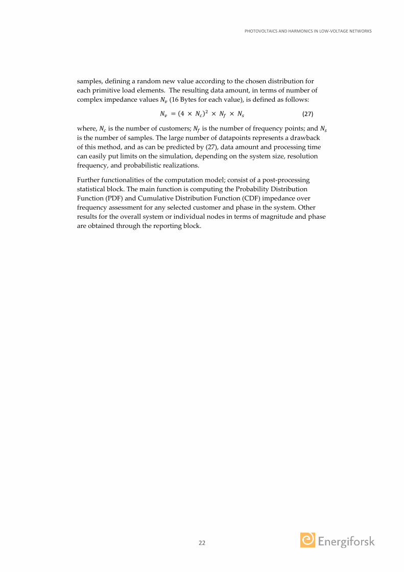
samples, defining a random new value according to the chosen distribution for each primitive load elements. The resulting data amount, in terms of number of complex impedance values 𝑁𝑁𝑣𝑣 (16 Bytes for each value), is defined as follows:

𝑁𝑁𝑣𝑣 = (4 × 𝑁𝑁𝑐𝑐)2 × 𝑁𝑁𝑒𝑒 × 𝑁𝑁𝑟𝑟 (27)

where, 𝑁𝑁𝑐𝑐 is the number of customers; 𝑁𝑁𝑒𝑒 is the number of frequency points; and 𝑁𝑁𝑟𝑟 is the number of samples. The large number of datapoints represents a drawback of this method, and as can be predicted by (27), data amount and processing time can easily put limits on the simulation, depending on the system size, resolution frequency, and probabilistic realizations.

Further functionalities of the computation model; consist of a post-processing statistical block. The main function is computing the Probability Distribution Function (PDF) and Cumulative Distribution Function (CDF) impedance over frequency assessment for any selected customer and phase in the system. Other results for the overall system or individual nodes in terms of magnitude and phase are obtained through the reporting block.


23

4 Low-Voltage Example Networks

To illustrate the model, it is applied to two Swedish networks. Both networks were selected based on criteria of complexity and application. Cable parameters (as defined in Section 2.1.5) for both networks are listed in Table 1.

The first network, illustrated in Figure 8, is a typical rural grid where a few houses spread over a few hundred meters, are connected to a single transformer. Detailed data is given in Table 2 and Table 3, where CB stands for “customer bus”.

The second network, shown in Figure 7, is a suburban grid with 28 customers connected to a 500 kVA transformer. This type of network is typical for a suburban region where some tens of houses are connected to the same distribution transformer. The data related to this network is presented in Table 4 and Table 5.

The source impedance at 10 kV is as follows:

For the 6-customer grid: 1.0736 + j 2.1325 Ω

For the 28-customer grid: 0.4174 + j 0.7977 Ω

The zero-sequence impedance of the transformer is assumed equal to the positive-sequence impedance.

Table 1. Cable and line impedances

Type Description 𝑺𝑺𝑺𝑺𝑺𝑺𝑺𝑺𝑺𝑺− 𝒄𝒄𝒄𝒄𝑺𝑺𝒄𝒄𝒄𝒄𝒄𝒄𝑺𝑺 𝒄𝒄𝒊𝒊𝒊𝒊𝒊𝒊𝒊𝒊𝒊𝒊𝒊𝒊𝒄𝒄𝒊𝒊 (𝑾𝑾/𝒌𝒌𝒊𝒊)

𝑬𝑬𝒊𝒊𝑺𝑺𝑺𝑺𝑺𝑺− 𝒇𝒇𝒊𝒊𝒄𝒄𝒇𝒇𝑺𝑺 𝒄𝒄𝒊𝒊𝒊𝒊𝒊𝒊𝒊𝒊𝒊𝒊𝒊𝒊𝒄𝒄𝒊𝒊 (Ω/𝒌𝒌𝒊𝒊)

𝑺𝑺𝒄𝒄𝑺𝑺𝒄𝒄𝒊𝒊𝒊𝒊𝑺𝑺𝒊𝒊𝒊𝒊𝒄𝒄𝒊𝒊 (µ𝑺𝑺/𝒌𝒌𝒊𝒊)

1 EKKJ-3x10/10 𝟏𝟏.𝟖𝟖𝟖𝟖𝟖𝟖 + 𝒋𝒋𝟖𝟖.𝟖𝟖𝟖𝟖𝟎𝟎 𝟖𝟖.𝟔𝟔𝟔𝟔𝟖𝟖 + 𝒋𝒋𝟖𝟖.𝟏𝟏𝟖𝟖𝟖𝟖 𝟗𝟗𝟗𝟗.𝟐𝟐𝟐𝟐

2 N1XE-4x10 𝟏𝟏.𝟖𝟖𝟖𝟖𝟖𝟖 + 𝒋𝒋 𝟖𝟖.𝟖𝟖𝟖𝟖𝟎𝟎 𝟖𝟖.𝟔𝟔𝟔𝟔𝟖𝟖 + 𝒋𝒋𝟖𝟖.𝟏𝟏𝟎𝟎𝟐𝟐 𝟖𝟖𝟏𝟏.𝟗𝟗𝟐𝟐

3 ALUS-4x25 𝟏𝟏.𝟐𝟐𝟖𝟖𝟖𝟖 + 𝒋𝒋 𝟖𝟖.𝟖𝟖𝟗𝟗𝟖𝟖 𝟐𝟐.𝟗𝟗𝟖𝟖𝟖𝟖 + 𝒋𝒋𝟖𝟖.𝟏𝟏𝟖𝟖𝟖𝟖 𝟏𝟏𝟐𝟐𝟖𝟖.𝟖𝟖𝟗𝟗

4 ALUS-4x50 𝟖𝟖.𝟔𝟔𝟗𝟗𝟏𝟏 + 𝒋𝒋 𝟖𝟖.𝟖𝟖𝟖𝟖𝟐𝟐 𝟏𝟏.𝟐𝟐𝟖𝟖𝟐𝟐 + 𝒋𝒋𝟖𝟖.𝟏𝟏𝟎𝟎𝟖𝟖 𝟏𝟏𝟐𝟐𝟎𝟎.𝟖𝟖𝟖𝟖

5 N1XV-4x50 𝟖𝟖.𝟔𝟔𝟗𝟗𝟏𝟏 + 𝒋𝒋 𝟖𝟖.𝟖𝟖𝟖𝟖𝟏𝟏 𝟏𝟏.𝟐𝟐𝟖𝟖𝟐𝟐 + 𝒋𝒋𝟖𝟖.𝟏𝟏𝟔𝟔𝟏𝟏 𝟖𝟖𝟏𝟏.𝟗𝟗𝟐𝟐

6 N1XE-4x50 𝟖𝟖.𝟔𝟔𝟗𝟗𝟏𝟏 + 𝒋𝒋 𝟖𝟖.𝟖𝟖𝟖𝟖𝟏𝟏 𝟏𝟏.𝟐𝟐𝟖𝟖𝟐𝟐 + 𝒋𝒋𝟖𝟖.𝟏𝟏𝟔𝟔𝟏𝟏 𝟖𝟖𝟏𝟏.𝟗𝟗𝟐𝟐

7 N1XE-4x150 𝟖𝟖.𝟐𝟐𝟖𝟖𝟔𝟔 + 𝒋𝒋 𝟖𝟖.𝟖𝟖𝟎𝟎𝟖𝟖 𝟖𝟖.𝟗𝟗𝟏𝟏𝟐𝟐 + 𝒋𝒋𝟖𝟖.𝟏𝟏𝟐𝟐𝟔𝟔 𝟖𝟖𝟏𝟏.𝟗𝟗𝟐𝟐

8 AKKJ-3x150/41 𝟖𝟖.𝟐𝟐𝟖𝟖𝟔𝟔 + 𝒋𝒋 𝟖𝟖.𝟖𝟖𝟎𝟎𝟗𝟗 𝟖𝟖.𝟔𝟔𝟗𝟗𝟗𝟗 + 𝒋𝒋𝟖𝟖.𝟖𝟖𝟎𝟎𝟔𝟔 𝟐𝟐𝟐𝟐𝟏𝟏.𝟖𝟖𝟖𝟖

9 AKKJ-3x240/72 𝟖𝟖.𝟏𝟏𝟐𝟐𝟐𝟐 + 𝒋𝒋 𝟖𝟖.𝟖𝟖𝟎𝟎𝟖𝟖 𝟖𝟖.𝟖𝟖𝟎𝟎𝟖𝟖 + 𝒋𝒋𝟖𝟖.𝟖𝟖𝟎𝟎𝟔𝟔 𝟐𝟐𝟖𝟖𝟐𝟐.𝟎𝟎𝟗𝟗

10 FKKJ-3x35/16 𝟖𝟖.𝟐𝟐𝟐𝟐𝟗𝟗 + 𝒋𝒋 𝟖𝟖.𝟖𝟖𝟎𝟎𝟗𝟗 𝟏𝟏.𝟔𝟔𝟎𝟎𝟗𝟗 + 𝒋𝒋𝟖𝟖.𝟖𝟖𝟖𝟖𝟔𝟔 𝟏𝟏𝟖𝟖𝟖𝟖.𝟐𝟐𝟖𝟖

11 N1XV-4x10 𝟏𝟏.𝟖𝟖𝟖𝟖𝟖𝟖 + 𝒋𝒋 𝟖𝟖.𝟖𝟖𝟖𝟖𝟎𝟎 𝟖𝟖.𝟔𝟔𝟔𝟔𝟖𝟖 + 𝒋𝒋𝟖𝟖.𝟏𝟏𝟎𝟎𝟐𝟐 𝟖𝟖𝟏𝟏.𝟗𝟗𝟐𝟐


24

Figure 7 Single-line diagram for the 28-Customer network

Figure 8 Single-line diagram for the 6-Customer network

Table 2. Transformer Data for the 6-Customer Network

Power 100 kVA Voltage 10/0.4 kV

Connection Dyn11

Positive sequence impedance 4 %

Source impedance at 10 kV 1.0736+j2.132Ω

Table 3. Cable and Line Data for the 6-Customer Network

N1 N2 Cable Length (m) N1 N2 Cable Length (m)

B2 B3 5 14.0 B7 B11 2 54.4

B3 B4 4 108.0 B7 CB5 1 8.9

B4 B5 4 26.9 B7 CB6 2 79.5

B4 B6 4 46.0 B8 CB1 1 41.5

B4 B7 3 1.9 B9 B10 3 0.1

B5 B8 4 41.2 B10 CB2 1 17.0

B5 B9 4 0.1 B11 CB4 1 41.3

B6 CB3 1 31.0

Slack bus B0

Utility grid

T10.5 MVA

10 / 0.4 kV

B18

CB24CB25

CB26

CB27CB28

B17B18

B14

CB17CB18

CB19

CB20

B15

B12

CB21CB22

CB23

CB15CB16

B13

B11

CB8

CB9

CB10CB11

B10B9

CB12CB13

CB14

B6

CB7

CB6B7B8

CB5B5 CB3

CB4B4CB1

CB2

B2B3

B1

B2

B4

B3

B5 B6 B7B8 B9

B10B11

CB1 CB2 CB3 CB4 CB5 CB6

Slack bus B1

Utility grid

T1100 kVA

10 / 0.4 kV


25

Table 4. Transformer Data for the 28- Customer Network

Power 500 kVA Voltage 10/0.4 kV

Connection Dyn11

Positive sequence impedance 4.9 %

Source impedance at 10 kV 0.4174+j0.797Ω

Table 5. Cable and Line Data for the 28-Customer Network

N1 N2 Cable Length (m) N1 N2 Cable Length (m)

B1 B2 7 15.0 B11 CB9 1 37.8

B2 B3 8 77.9 B1 B12 8 196.9

B3 CB1 1 68.7 B12 CB21 1 33.8

B3 CB2 1 24.9 B12 CB22 1 65.7

B3 B4 8 56.0 B12 CB23 1 17.0

B4 CB3 1 22.4 B12 B13 10 89.5

B4 CB4 1 48.9 B13 CB15 1 42.7

B4 B5 8 64.1 B13 CB16 1 27.7

B5 CB5 1 28.2 B12 B14 10 71.0

B5 B6 8 67.4 B14 CB20 1 21.2

B6 CB6 1 23.1 B14 B15 10 58.6

B6 B7 8 52.3 B15 CB17 11 28.9

B7 B8 7 1.2 B15 CB18 11 21.7

B8 CB7 6 34.2 B15 CB19 11 33.0

B1 B9 9 270.1 B1 B16 8 157.0

B9 CB12 1 29.8 B16 B17 8 50.6

B9 CB13 1 46.1 B17 CB28 1 22.9

B9 CB14 1 23.4 B17 CB27 1 41.8

B9 B10 8 86.0 B17 B18 10 93.4

B10 CB10 1 47.2 B18 CB24 1 76.2

B10 CB11 1 27.7 B18 CB25 1 37.4

B10 B11 10 96.1 B18 CB26 1 28.5

B11 CB8 1 29.9


26

5 Emission from PV and from domestic customers

Harmonics are injected into the grid, not only by inverters but from common household equipment as well (computers, microwave ovens, energy efficient lights to name a few). The current harmonics for the three individual phases measured at a number of customers, without PV installation, during one week is shown Figure 9, Figure 10 and Figure 11. As can be seen in the figures, the current harmonic emission varies between customers and between phases. The spectra and corresponding magnitudes depends on what type of equipment a customer has connected at that certain moment in time.

Figure 9 Current harmonics measured at customer A. P95% (top), maximum (middle), and minimum (bottom) values over one week, 10 minutes average of the individual RMS current harmonics for phases a, b and c, measured at the delivery point.

Figure 10 Current harmonics measured at customer B. P95% (top), maximum (middle), and minimum (bottom) values over one week, 10 minutes average of the individual RMS current harmonics for phases a, b and c, measured at the delivery point.


27

Figure 11 Current harmonics measured at customer C. P95% (top), maximum (middle), and minimum (bottom) values over one week, 10 minutes average of the individual RMS current harmonics for phases a, b and c, measured at the delivery point.

Harmonic emission from a domestic customer varies during the day as the costumer use different household devices. The highest values tend to occur during the evening as seen in Figure 12 where the average hourly THDI during one week measured at customer C is shown. The average power consumption for customer C during the week was 0.44 kW divided between the three phases and the peak consumption was 2.0 kW for phase a and b and 1.2 kW for phase c.

Figure 12 Hourly average THDI during one week for customer C during one week. Different colors represent the three phases

The emission from PV inverters has to be related to the contribution from other loads. In Figure 13 the hourly average THDI from a 2.5 kW single phase PV installation is shown. The absolute value of the peak production is somewhat


28

comparable to the per phase peak consumption of customer C shown in Figure 12 but occurs during the day. As seen when comparing the highest values shown in Figure 12 and Figure 13, the worst case (highest THDI) occurs not during production from the PV installation but during evening for the domestic customer without PV installation. This difference in time of day for the peak in emission indicates that the emission contributed from the PV inverter will not add to the background emission in any significant way.

Figure 13 Hourly average THDI during one week of production for a 2.5 kW single phase PV installation


29

6 Stochastic Modelling of Transfer Impedances

The adjustment of the simulation model was based on studies described in [4], [5], [6], [7], and [8], and based on some assumptions described in the following.

6.1 ABOUT THE RLC RANGE FOR THE LOAD/CO-GENERATION MODEL

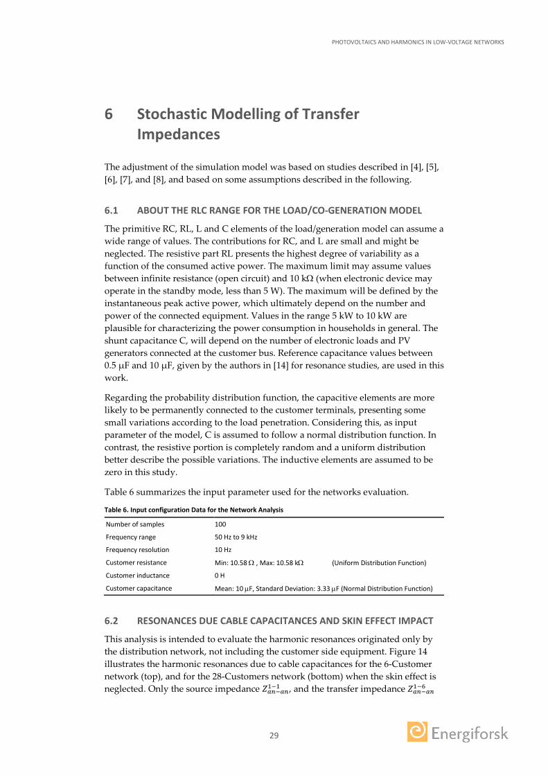
The primitive RC, RL, L and C elements of the load/generation model can assume a wide range of values. The contributions for RC, and L are small and might be neglected. The resistive part RL presents the highest degree of variability as a function of the consumed active power. The maximum limit may assume values between infinite resistance (open circuit) and 10 kΩ (when electronic device may operate in the standby mode, less than 5 W). The maximum will be defined by the instantaneous peak active power, which ultimately depend on the number and power of the connected equipment. Values in the range 5 kW to 10 kW are plausible for characterizing the power consumption in households in general. The shunt capacitance C, will depend on the number of electronic loads and PV generators connected at the customer bus. Reference capacitance values between 0.5 µF and 10 µF, given by the authors in [14] for resonance studies, are used in this work.

Regarding the probability distribution function, the capacitive elements are more likely to be permanently connected to the customer terminals, presenting some small variations according to the load penetration. Considering this, as input parameter of the model, C is assumed to follow a normal distribution function. In contrast, the resistive portion is completely random and a uniform distribution better describe the possible variations. The inductive elements are assumed to be zero in this study.

Table 6 summarizes the input parameter used for the networks evaluation.

Table 6. Input configuration Data for the Network Analysis

Number of samples 100

Frequency range 50 Hz to 9 kHz

Frequency resolution 10 Hz

Customer resistance Min: 10.58 Ω , Max: 10.58 kΩ (Uniform Distribution Function)

Customer inductance 0 H

Customer capacitance Mean: 10 µF, Standard Deviation: 3.33 µF (Normal Distribution Function)

6.2 RESONANCES DUE CABLE CAPACITANCES AND SKIN EFFECT IMPACT

This analysis is intended to evaluate the harmonic resonances originated only by the distribution network, not including the customer side equipment. Figure 14 illustrates the harmonic resonances due to cable capacitances for the 6-Customer network (top), and for the 28-Customers network (bottom) when the skin effect is neglected. Only the source impedance 𝑍𝑍𝑎𝑎𝑎𝑎−𝑎𝑎𝑎𝑎1−1 , and the transfer impedance 𝑍𝑍𝑎𝑎𝑎𝑎−𝑎𝑎𝑎𝑎1−6


30

are analyzed. The resonance frequencies are calculated according to (1), dependent on the combination of cable capacitances and transformer-cable inductances.

Figure 14 Resonances due cable capacitances only, without skin effect for 6-Customer network (top) and 28-customers network (bottom).

Although it is a hypothetical and unlikely situation to happen in real systems, this result helps to understand how the resonances are spread over the frequency, even in the high-frequency range. As can be observed, the number of resonance frequencies is dependent of the number and length of the feeders. This is only possible because the capacitances are radially connected and there is no great disparity among the cable capacitances, otherwise a predominant resonance would overlap the others. The common predominant inductance comes from the transformer.

Once the skin effect is considered the impedance versus frequency drastically changes. Figure 15 shows the same impedance versus frequency illustrated in Figure 14 damped by the skin effect.

Figure 15 Resonances due cable capacitances only, considering skin effect for 6-Customer network (top) and 28-customers network (bottom).


31

From the results depicted in Figure 14, is possible to verify that the peak values decreased by 10. Low-frequency resonances due the predominant capacitances still appears, while high-frequency resonances almost disappeared due the increasing of the resistance at high-frequencies because of the skin effect.

6.3 OVERALL SYSTEM NETWORK TRANSFER IMPEDANCE

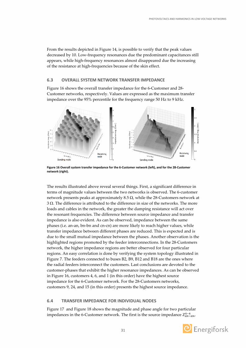
Figure 16 shows the overall transfer impedance for the 6-Customer and 28-Customer networks, respectively. Values are expressed as the maximum transfer impedance over the 95% percentile for the frequency range 50 Hz to 9 kHz.

Figure 16 Overall system transfer impedance for the 6-Customer network (left), and for the 28-Customer network (right).

The results illustrated above reveal several things. First, a significant difference in terms of magnitude values between the two networks is observed. The 6-customer network presents peaks at approximately 8.5 Ω, while the 28-Customers network at 3 Ω. The difference is attributed to the difference in size of the networks. The more loads and cables in the network, the greater the damping resistance will act over the resonant frequencies. The difference between source impedance and transfer impedance is also evident. As can be observed, impedance between the same phases (i.e. an-an, bn-bn and cn-cn) are more likely to reach higher values, while transfer impedance between different phases are reduced. This is expected and is due to the small mutual impedance between the phases. Another observation is the highlighted regions promoted by the feeder interconnections. In the 28-Customers network, the higher impedance regions are better observed for four particular regions. An easy correlation is done by verifying the system topology illustrated in Figure 7. The feeders connected to buses B2, B9, B12 and B18 are the ones where the radial feeders interconnect the customers. Last conclusions are devoted to the customer-phases that exhibit the higher resonance impedances. As can be observed in Figure 16, customers 4, 6, and 1 (in this order) have the highest source impedance for the 6-Customer network. For the 28-Customers networks, customers 9, 24, and 15 (in this order) presents the highest source impedance.

6.4 TRANSFER IMPEDANCE FOR INDIVIDUAL NODES

Figure 17 and Figure 18 shows the magnitude and phase angle for two particular impedances in the 6-Customer network. The first is the source impedance 𝑍𝑍𝑎𝑎𝑎𝑎−𝑎𝑎𝑎𝑎4−4 ,


32

and the second is the transfer impedance 𝑍𝑍𝑎𝑎𝑎𝑎−𝑏𝑏𝑎𝑎1−4 between customers 1 and 4, for different phases.

Figure 17 6-Customers network, source impedance phase angle 𝒁𝒁𝒊𝒊𝒊𝒊−𝒊𝒊𝒊𝒊𝟗𝟗−𝟗𝟗 (left), and transfer impedance phase 𝒁𝒁𝒊𝒊𝒊𝒊−𝒃𝒃𝒊𝒊𝟏𝟏−𝟗𝟗 (right).

Figure 18 6-Customers network, source impedance magnitude 𝒁𝒁𝒊𝒊𝒊𝒊−𝒊𝒊𝒊𝒊𝟗𝟗−𝟗𝟗 (left), and transfer impedance magnitude 𝒁𝒁𝒊𝒊𝒊𝒊−𝒃𝒃𝒊𝒊𝟏𝟏−𝟗𝟗 (right).

Figure 19 28-Customers network, source impedance phase angle 𝒁𝒁𝒊𝒊𝒊𝒊−𝒊𝒊𝒊𝒊𝟗𝟗−𝟗𝟗 (left), and transfer impedance phase 𝒁𝒁𝒊𝒊𝒊𝒊−𝒃𝒃𝒊𝒊𝟗𝟗−𝟐𝟐𝟖𝟖 (right).

Figure 20 28-Customers network, source impedance magnitude 𝒁𝒁𝒊𝒊𝒊𝒊−𝒊𝒊𝒊𝒊𝟗𝟗−𝟗𝟗 (left), and transfer impedance magnitude 𝒁𝒁𝒊𝒊𝒊𝒊−𝒃𝒃𝒊𝒊𝟗𝟗−𝟐𝟐𝟖𝟖 (right).

As can be seen in Figure 18, for the source impedance 𝑍𝑍𝑎𝑎𝑎𝑎−𝑎𝑎𝑎𝑎4−4 , a resonance frequency centered at 1.3 kHz is the dominant one. The minimum impedance magnitude is 5.4 Ω, while the 95th percentile is 9.3 Ω. For this network, the impedance easily exceeds the reference limit given by IEC 61000-4-7.

Comparing these results with the results found in similar studies (e.g. [5] and [6]), the resonant frequency is approximately the same as found in some German distribution networks but with different magnitudes. The difference can be explained because in this network, due to few customers, the number of resistive


33

loads may be reduced in average and therefore less damping is present at the resonance frequency.

A different situation occurs for the transfer impedance 𝑍𝑍𝑎𝑎𝑎𝑎−𝑏𝑏𝑎𝑎1−4 (different customers, and different phases), where the resonant frequency is approximately 1.25 kHz, and the magnitude is significantly less compared to 𝑍𝑍𝑎𝑎𝑎𝑎−𝑎𝑎𝑎𝑎4−4 . However, although the magnitude is reduced, there is a resonance frequency for the transfer impedance between customers. This means that harmonics originally present with one customer can be amplified by the resonance and injected to parallel phases and other customers within the same network.

Regarding phase angle (shown in Figure 19), changes are observed around the resonance frequency. Those changes can contribute to harmonic cancellation as well as result in amplification. Further studies are needed in this field to obtain a better understanding.

The magnitude for two node impedances for the 28-Customer network is illustrated in Figure 20, similar to the previous analysis for the 6-Customer network. The first is the source impedance 𝑍𝑍𝑎𝑎𝑎𝑎−𝑎𝑎𝑎𝑎9−9 (higher source impedance), and the second is the transfer impedance 𝑍𝑍𝑎𝑎𝑎𝑎−𝑏𝑏𝑎𝑎9−28 between customers 1 and 4, for different phases.

From the results presented in Figure 20, the first observation is that the resonance impedance does not exceed the limit given by IEC 61000-4-7. Another result from this network is the presence of two resonance impedances. The higher resonance impedance, for both, source impedance 𝑍𝑍𝑎𝑎𝑎𝑎−𝑎𝑎𝑎𝑎9−9 , and transfer impedance 𝑍𝑍𝑎𝑎𝑎𝑎−𝑏𝑏𝑎𝑎9−28 , is close to 0.74 kHz, and the magnitude is approximately 2.8 Ω.

Regarding phase angle (Figure 19), specifically for the source impedance 𝑍𝑍𝑎𝑎𝑎𝑎−𝑎𝑎𝑎𝑎9−9 , an expressive change is noticed in the harmonic range due the resonance frequency, following by a stable condition up to 5 kHz.


34

7 Impact of PV on the Transfer Impedances

The impact of PV installations on the transfer impedance is presented in this Chapter. The same approach as described in Chapter 6 has been used and PV inverters modeled as shunt capacitances have been added to the model at different customer sites. Load configuration for Monte Carlo simulation was used considering 1000 samples. For each realization, individual RLC elements, connected between phase and neutral on each phase, were randomly selected. Inductances were fixed to zero for all phases, resistances were randomly selected from 16 Ω up to 32 kΩ (i.e. active power ranging from 10 kW to 5 W approximately) from a uniform probability distribution, and load capacitances were randomly selected from a normal probability distribution with mean of 5 µF, and standard deviation of 1.5 µF. Capacitance from inverter, with values of 5, 10, 15 and 20 µF are randomly added to phases using a discrete uniform distribution. The results presented in Figure 21 show individual samples for the magnitude of the transfer impedances between customer 1 and customer 2 (phase a) up to 9 kHz for the 6-Customer network without PV inverters. Monte Carlo simulation was performed keeping the network fixed and varying customer loads. In Figure 22 the same conditions were kept but PV inverters have been added at the customer sites. The overall values of the impedance are reduced but the resonance is shifted towards the lower frequency range. Statistical results for the transfer impedances under analysis are shown in Figure 23 and Figure 24 without and with PV inverters, respectively.

Figure 21 6-Customer network Monte Carlo transfer impedance Zan1-an2 in the absence of PV inverters.


35

Figure 22 6-Customer network Monte Carlo transfer impedance Zan1-an2 in the presence of PV inverters.

Figure 23 6-Customer network transfer impedance Zan1-an2 in the absence of PV inverters.

Figure 24 6-Customer network transfer impedance Zan1-an2 in the presence of PV inverters.


36

In Figure 25 and Figure 26 the results for the 28 customer network is shown. Compared to the 6 customer network, the impedance values are lower but also in this case the introduction of PV inverters causes the resonance to be shifted to a lower frequency and an overall decrease of impedance values.

Figure 25 28-Customer network transfer impedance Zan1-an9, in the absence of PV inverters.

Figure 26 28-Customer network transfer impedance Zan1-an9, in the presence of PV inverters.

The overall maximum CP95 magnitude of the transfer impedances up to 9 kHz for the 6-Customer network without PV inverters is shown in Figure 27. To better highlight magnitude variations, the transfer impedances are illustrated in two groups: transfer impedance at the same phase (a) and between different phases (b). Monte Carlo simulation using the same procedure previously described was used.


37

Figure 27 6-Customer network without PV inverters. Maximum CP95 of the transfer impedance magnitude at the same phase (a), between different phases (b).

Results presented in Figure 27 show that when there are no inverters connect to any customer, the maximum transfer impedance, at the resonance frequency, for the same phase, are on average 3.7 times greater than the maximum transfer impedance between different phases. This difference is expected since only series neutral impedances, and shunt phase impedances are considered for the total impedances between phases, while for impedances on the same phase, all series and mutual contributions are considered. The overall maximum impedance, at the resonance frequency, is observed for the customer 8, phase an, with magnitude of 10.61 Ω. For transfer impedance between phases, it reaches the maximum magnitude also at customer 8, between phases an and bn, with magnitude of 2.85 Ω. In this case, both maxima are at the same customer because customer 8 presents the larger cable impedance from the common connection bus for all customers (bus 3).

The overall frequency at the maximum CP95 magnitude of the transfer impedances up to 9 kHz for the 6-Customer network with PV inverters is shown in Figure 28.

Figure 28 6-Customer network without PV inverters. Frequency of the maximum CP95 of the transfer impedance magnitude at the same phase (a), between different phases (b).

Considering no inverters connected to any customer, results show that the frequency for the overall resonance frequency occurs in the range between 1.9 kHz


38

and 2.05 kHz for the transfer impedances at the same phase, and between 1.50 kHz and 1.95 kHz for transfer impedances between different phases.

On average, the resonant frequency for impedances between different phases is 13% less than the resonant frequency for impedances on the same phase. The difference is attributed to variations, both for the inductive and capacitive reactance over the conductors. For the inductive reactance, the gain in frequency for transfer impedances between different phases is less compared to transfer impedance on the same phase. This occurs mainly because the series impedances, when there is no phase in common, are less than when one phase is shared between two points. The capacitive reactance reacts inversely. When there are two phases involved, besides the neutral capacitances, the two individual capacitive contributions for each phase are summed. As a result, the gain will be higher and inversely proportional to frequency compared to the capacitive reactance when only one phase is considered. Comparing one phase with two phases, inductive reactance will increase the frequency, and the capacitive reactance will decrease the frequency, but with a greater proportion. In the end, the effect of variations in the inductive reactance is suppressed by variations in the capacitive reactance what explains why the frequency decreases when comparing impedances on the same phase and between two phases.

PV inverters were randomly added to all customers and the overall maximum CP95 magnitude of the transfer impedances up to 9 kHz for the 6-Customer network with PV inverters is shown in Figure 29 (cf. Figure 27).

Figure 29 6-Customer network with PV inverters. Maximum CP95 of the transfer impedance magnitude at the same phase (a), between different phases (b).

Considering inverters being randomly connected to customer, results show that the magnitude for the overall resonant frequency occurs in the range between 3.2 Ω and 4.9 Ω for the transfer impedances at the same phase, and between 0.8 Ω and 1.3 Ω for transfer impedances between different phases. Compared to the scenario without inverters, illustrated in Figure 27, magnitude is about 57 % less than the scenario with inverters. Since there is more capacitance connected to phases, the predominant capacitive reactance will decrease faster with the increase in frequency and as a result magnitude will decrease proportionally. The same reason can be attributed to the magnitude difference between impedance on one phase and two phases. When two phases are involved, more capacitance is added, and


39

the result will be a decrease in magnitude. The overall maximum impedance, at the resonance frequency, is observed for the customer 8, phase cn, with magnitude of 5.2 Ω. For transfer impedance between phases, it reaches the maximum magnitude also for customer 8, between phases an and bn, with magnitude of 1.31 Ω. In this case, as with the case without inverters, both maxima have in common customer 8 because it presents the largest cable impedance from the common connection bus for all customers (bus 3).

Overall frequency at the maximum CP95 magnitude of the transfer impedances up to 9 kHz for the 6-Customer network with PV inverters is shown in Figure 30 (cf. Figure 28).

Figure 30 6-Customer network with PV inverters. Frequency of the maximum CP95 of the transfer impedance magnitude at the same phase (a), between different phases (b).

Considering inverters being randomly connected to the customers, results show that the frequency for the overall resonance occurs in the range between 1.0 kHz and 1.06 kHz for the transfer impedances at the same phase, and between 0.7 kHz and 0.95 kHz for transfer impedances between different phases.

On average, the resonant frequency for impedances between different phases is 20% less than the resonant frequency for impedances on the same phase. Compared to the scenario without inverters frequency is about 50 % less, decreasing from about 2 kHz to 1 kHz. The reasons behind the decrease in frequency are the same reasons why the magnitude decreases.

Similar calculations have been done for the 28-customer network and the results are shown in Figure 31 to Figure 34.


40

Figure 31 28-Customer network without PV inverters. Maximum CP95 of the transfer impedance magnitude at the same phase (a), between different phases (b).

Figure 32 28-Customer network without PV inverters. Frequency of the maximum CP95 of the transfer impedance magnitude at the same phase (a), between different phases (b).

Figure 33 28-Customer network with PV inverters. Maximum CP95 of the transfer impedance magnitude at the same phase (a), between different phases (b).


41

Figure 34 28-Customer network with PV inverters. Frequency of the maximum CP95 of the transfer impedance magnitude at the same phase (a), between different phases (b).

Figure 35 (no PV inverters) and Figure 36 (with PV inverters) illustrate the Cumulative Distribution Function for the transfer impedance Zan1-an2 for frequencies up to 2 kHz, using the same Monte Carlo settings described earlier. As can be observed, in the absence of PV inverters, for less than 50% of the cases, resonance impedance tends to be with magnitudes higher than 6 Ω and located above 2 kHz. As the probability increases, both magnitude and frequency decrease. For 95% of the cases, resonant frequencies and peak magnitudes are close to 1.8 kHz and 4 Ω respectively. Once PV inverters are added, frequency and magnitude decrease. Maximum magnitudes of 4 Ω at 1.2 kHz are reached only in less than 10 % of the cases. For most of the cases (higher than 95%) resonant frequencies and peak magnitudes are close to 0.9 kHz and 2.5 Ω. Comparing both cases, the results illustrate how the impedances change with the increase of capacitances in the system. The reduction in frequency and magnitude from the case with absence of PV inverters and the case with presence of PV inverters is mainly attributed to the change of the intersection point between the dominant inductive reactance and capacitive reactance. The higher the capacitance in the system, the lower the frequencies and magnitudes will be for the resonant frequencies.

Figure 35 CDF up to 2 kHz of the transfer impedance magnitude for the 6-Customer network without PV inverters.


42

Figure 36 CDF up to 2 kHz of the transfer impedance magnitude for the 6-Customer network with PV inverters.

For the 6 customer network, the random connection of PV inverters at the customer sites will result in an average decrease in impedance magnitude of about 57%. Magnitude for the overall resonant frequency occurs in the range between 3.2 Ω and 4.9 Ω for individual customers as seen in Figure 29 (7.9 Ω and 10.9 Ω without inverters) for the transfer impedances at the same phase, and between 0.8 Ω and 1.3 Ω (2.10 Ω and 2.85 Ω without inverters) for transfer impedances between different phases. Overall resonant frequency occurs in the range between 1.0 kHz and 1.06 kHz (1.90 kHz and 2.05 kHz without inverters) for the transfer impedances at the same phase, and between 0.7 kHz and 0.95 kHz (1.50 kHz and 1.95 kHz without inverters) for transfer impedances between different phases. On average, the resonant frequency for impedances between different phases is 20% less than the resonant frequency for impedances on the same phase.

For the 28 customer network the randomly connection of PV inverters at the customer sites will result in an average decrease in impedance magnitude of about 70%. Magnitude for the overall resonant frequency occurs in the range between 1.0 Ω and 1.9 Ω (2.75 Ω and 6.5 Ω without inverters) for the transfer impedances at the same phase, and between 0.2 Ω and 0.1.25 Ω (0.9 Ω and 2.0 Ω without inverters) for transfer impedances between different phases. Overall resonant frequency occurs in the range between 0.82 kHz and 10 kHz (1.5 kHz and 1.55 kHz without inverters) for the transfer impedances at the same phase, and between 0.62 kHz and 4.5 kHz (1.34 kHz and 7.96 kHz without inverters) for transfer impedances between different phases.

Although some resonant frequencies may reach high values in some situations (e.g. 10 kHz and 4.5 kHz), this happens in a reduced number of impedances in the system. As can be seen in Figures 28-b, 30-a and 30-b, the transfer impedances related to customers 1 to 7 tend to have higher values for resonant frequency. This is a result of the presence of more than one resonant frequency (i.e. above 2 kHz), which does not mean that the harmonics range is not affected. Most consumers will experience resonant frequencies in the order of 0.82 kHz (1.5 kHz without inverters) for the transfer impedances at the same phase, and 0.62 kHz (1.34 kHz


43

without inverters) for transfer impedances between different phases. One of the reasons that can explain this behavior is the low attenuation due to the low resistivity of the cables since these customers are located near the substation. However other factors may also have influence, and further studies need to be carried out on this issue.


44

8 Impact of PV on voltage distortion

The connection of PV inverters has an impact on the impedance in the grid at harmonic frequencies as described in Chapter 7. For this to become an issue there also has to be emission at those frequencies, i.e. how the current emission injected by the inverter effect the voltage distortion is dependent on the impedance of the grid at that frequency. As shown in Chapter 5 the highest values of current harmonic emission are due to normal household devices and those values have been used to investigate the impact on voltage distortion. The current harmonic emissions have been used to calculate the resulting voltage distortion given the transfer impedance for increasing numbers of PV inverters in the two sample networks. To account for the aggregation effect the method described in IEC 61000-3-6 is used (28).

𝑈𝑈ℎ = 𝑈𝑈ℎ𝑖𝑖𝛼𝛼𝑖𝑖

𝛼𝛼 (28)

Where 𝑈𝑈ℎ is the magnitude of the resulting voltage harmonic (order h), 𝑈𝑈ℎ𝑖𝑖 is the magnitude of the various individual emission levels (order h) to be combined and α is the summation exponent according to Table 7.

Table 7. Summation exponent defined in IEC 61000-3-6 for different harmonic orders

Harmonic order α

h < 5 1

5 ≤ h ≤ 10 1.4

h > 10 2

The result for the 6 customer network is shown in Figure 37 where the resulting voltage THD in percent of fundamental is presented. In Figure 37 all customers are assumed to have the same current harmonic injection (as presented in Figure 9) and PV inverters are added randomly to the phases. The difference in voltage THD between customers is thus due to the different impedance seen at individual customers connection point. The voltage THD is increasing for all customers as the number of PV inverters installed in the network increases. The highest value is found at customer 4 and the voltage THD is increased with 0.27% between the zero inverter case to the six inverter case for this customer. The voltage THD limit in EN 50160 at 8% will not be violated.


45

Figure 37 6-Customers network THD considering the increasing of randomly connected PV inverter penetration, using CP95% for current harmonics as measured at customer A and transfer impedance. Colours indicate the different customers within the network.

The increasing in voltage THD can be attributed to the reduction in resonant frequency, as PV inverters are added, resulting in increasing the overall capacitance. As the resonance frequency shifts to the range below 500 Hz, the aggregation exponent α for the voltage distortion computation will be higher (α equal to 1.4 between 5th to 10th harmonics), and as a result cancellation will be less. The situation becomes worse when the impedance begins to increase below the 4th harmonic. In that case, summation exponent is further reduced (no cancellation at all between 2nd - 4th harmonics), resulting in higher THD values, even though the peak resonance frequency does not reach that frequency range.

The exercise was repeated and the PV inverters were in this case all connected to phase a (as oppose to Figure 37 where the connation was random) and the result is shown in Figure 38. Again the highest values are found for customer 4 and the difference between the phases is greater compared to random connection of the inverters. The distortion in phase a is effected most and the voltage THD at all customers increase with increasing number of inverters independent of location of connection. The impact on phase b and phase c is minor.


46

Figure 38 6-Customer network THD considering increasing of PV inverter penetration in phase a, using CP95% for current harmonics as measured at customer A and transfer impedance. Colours indicate the different customers within the network.

In Figure 39 the impact on an individual harmonic, harmonic 19, which is close to the expected resonant frequency, is shown. The calculation is done in a similar way as the previous examples i.e. representative CP95% values measured at customer A were used as reference for all customers and PV inverters were randomly connected to the different phases.

Figure 39 6-Customer network h19 considering increasing PV inverter penetration, using CP95% values for current harmonics and transfer impedance.

As can be observed there is a slight increase in the harmonic level for all phases as the number of PV inverters increases. More inverters in the system mean more shunt capacitances. Consequently, the resonance frequency for the overall transfer impedance will shift from high to low frequency range, resulting in more voltage amplification close to the 19th harmonic. In this particular case, the shifting to low frequency resulted in an increase of about 15% in the 19th harmonic. Although it is


47

a small contribution, depending to the current harmonics level, this increase may lead to an excessive increase in order of harmonics previously considered less important.

In Figure 40 and Figure 41 the impact on voltage THD for the 28 customer network is shown. There are no significant changes in the THD as PV inverters are added to system. One possible reason for that is because the resonant impedance moves inside the 0-2 kHz range, even without any PV inverter. In this case, only the shunt capacitances from electronic loads can push the resonance impedance below 2 kHz. The additional increase in PV inverters will add more capacitance to the system moving the resonant frequency to lower frequencies, but still inside the harmonic range. In conclusion, for this network, the impedance movement can change individual harmonics, but in average THD will be little affected.

Figure 40 28-Customer network THD considering increasing PV inverter penetration, using CP95% for current harmonics and transfer impedance.

Figure 41 28-Customer network THD considering increasing PV inverter penetration only at phase an, using CP95% values for current harmonics and transfer impedance

In Figure 42 the impact on the 19th harmonic as PV inverters are added at the 28 customer network is shown. Results show that an increasing number of PV inverters in the system can result in an increase of up to 43% on the 19th harmonic on some phases. The maximum value of 0.40% of fundamental is reached when 16


48

inverters are connected. As the resonant impedance shifts from high to low frequency range, the 19th harmonics is amplified progressively until it reaches the maximum value. At that condition, the resonant impedance frequency is about 950 Hz and voltage amplification is at its maximum. After that condition, the resonant impedance frequency moves to lower frequencies and voltage amplification decreases.

Figure 42 28-Customer network h19 considering increasing PV inverter penetration, using CP95% values for current harmonics and transfer impedance.

In Figure 43 individual voltage harmonics for one phase at customer 1 are shown, again calculated using the transfer impedance for the 6 customer network, considering current harmonic emission for customer A (as shown in Figure 9) and no PV inverters.

Figure 43 6-Customer network harmonics voltage for customer 1, phase bn, considering CP95% of current injections, and CP95% of the overall transfer impedance, in the absence of PV inverters

In Figure 44 the impact of the connection of PV inverters is shown, the same condition as in Figure 43 is otherwise used i.e. same customer, same phase, same current emission.


49

The shift to a lower resonant point compared to Figure 43 is seen in Figure 44, the resonant frequency in this case coincides with harmonic 20. The impact on the voltage harmonics close to this resonance is however minor as the absolute value of the impedance isn’t significantly affected (note the difference in the right vertical scale between the figures).

Figure 44 6-Customer network harmonics voltage for customer 1, phase bn, considering CP95% of current injections, and CP95% of the overall transfer impedance, in the presence of PV inverters.

The impact is most significant for the higher frequency range where the impedance is lowered by the connection of the inverters with a lower voltage harmonic magnitude as a result as shown in Figure 45. For the odd harmonics there is a decrease for all harmonics except h5, h7, h11, h13, h17 and h19.

Figure 45 6 customer network with PV connected (blue bars) and without PV (grey bars)

The same calculation has been done for the 28 customer network and the results are shown in Figure 46, Figure 47 and Figure 48.


50

Figure 46 28-Customer network harmonic voltage for customer 1, phase bn, considering CP95% of current injections, and CP95% of the overall transfer impedance, in the absence of PV inverters.

Figure 47 28-Customer network harmonics voltage for customer 1, phase bn, considering CP95% of current injections, and CP95% of the overall transfer impedance, in the presence of PV inverters.

Similar to the 6 customer network the impact is most significant for the upper frequency range, again with a reduction in voltage harmonic magnitude as seen in Figure 48. For the odd voltage harmonics the biggest amplification is at h17 which increases with 51%. Worth emphasizing is that even with this amplification the magnitude only reaches 0.44% of the fundamental which is well below the limit at 2% in EN 50160.


51

Figure 48 28 customer network with PV connected (blue bars) and without PV (grey bars)

Considering only electronic loads connected, simulation results have shown that the 6-Customer network has the resonance frequency above the 2-kHz range, meaning a low degree of impact in the harmonic range. For the 28-Customer network, due to the greater amount of shunt capacitances, the resonant impedance can occur below the 2-kHz range, for instance between 29th and 33th harmonics.

Considered PV penetration, both networks will be affected, although to a different degree, both networks mainly on the voltage harmonics between 17th and 21st orders.


52

9 Supraharmonics and PV

PV inverters are a source of supraharmonics (waveform distortion in the frequency range between 2 and 150 kHz) as shown in e.g. [14-18]. From a large number of measurements done primarily in Sweden and Germany it is seen that the emission from small single phase connected PV inverters (installed power below 4.6 kW) occurs at frequencies somewhere in the range between 15 kHz and 20 kHz. For three phase connected inverters used for higher power units the switching often takes place at a lower frequency range starting at around 2 kHz as seen in Table 8. More recently smaller three phase inverters started to appear on the market with switching frequencies around 20 kHz. Supraharmonic emission can be seen in the current as long as the PV is producing power. As most inverters are equipped with filters that are connected as long as the inverter is connected (i.e. also during times of no production) supraharmonics produced elsewhere can flow towards the inverter, so called secondary emission [19].

Table 8. Dominating supraharmonic component measured at various installations [15]

Installation Single phase roof top, 1.5 kW

Single phase roof top, 4.6 kW

Single phase roof top, 2.5 kW

Three phase, 20 kW

Three phase, 10 kW

Three phase 100 kW, part of a plant of 6.4 MW PV plant (50 Hz system)

Three phase, 1 MW PV plant, measured at the interface to the utility (60 Hz system)

Three phase, 100 kW

Dominating supraharmonic frequency

16.7 kHz

16.6 kHz

16 kHz 3.8 kHz 20 kHz 4 kHz ± 100 Hz

4 kHz ± 120 Hz 3 kHz

The transfer and aggregation of supraharmonics is significantly different from the transfer and aggregation of harmonics. As described in [20, 21] supraharmonics tend to propagate towards neighbouring devices and only a small part will propagate towards the grid. The impact from neighbouring devices is hence dominating and resonances play a significant part, not only in how supraharmonics propagate but also on the magnitude of the emission coming from a device. The latter is illustrated in Figure 49 where measurements from a PV inverter and a heat pump are shown. On the left hand side of the figure the device is connected alone and the components seen at 16 kHz (PV) and at 18 kHz (heat pump) are due to the switching circuit in the device. The influence from neighbouring devices is shown on the right hand side in Figure 49 where the magnitude of the component is increased (two and five times for the inverter and heat pump respectively) as other devices are connected nearby. This is likely the result from the two devices acting like voltage sources and a series resonance in the system.


53

Figure 49 Supraharmonics from a PV inverter connected alone (upper left), the same inverter while neighbouring devices are connected (upper right). A heat pump connected alone (lower left), the same heat pump while neighbouring devices are connected (lower right).

As shown in Chapter 6 and in [20] the likelihood of resonances forming in the frequency range between 2 and 150 kHz is high. As the supraharmonic emission from PV inverters is predominantly in the range between 2 and 20 kHz an amplification of this emission is also likely to occur. To model supraharmonics is not straightforward for several reasons, the dominating impact from neighbouring equipment and the time/frequency varying nature of the emission being the main ones. While harmonic sources can be modelled as current sources this is not always the case for supraharmonics as they can behave as a voltage source, a current source or both. The magnitude and frequency of the emission from most household devices varies within a timeframe of one cycle of the power system frequency (20 ms), two examples can be seen in Figure 50, where the Short Time Fourier Transform of a fluorescent lamp and a heat pump are shown. The emission from the fluorescent lamp varies in frequency and in magnitude during 20 ms whereas the emission from the heat pump varies only in amplitude as it appears and disappears four times per cycle. The impedance seen by a supraharmonic source is dominated by neighboring devices as they tend to offer a low impedance path for supraharmonic currents. Measurements presented in [20] show that a significant amount of supraharmonic currents produced by normal household devices propagate to the terminal of a PV inverter connected within the same customer site. The consequences for the PV inverters have yet to be investigated. Depending on type of load, this impedance introduced by household devices can


54

change significantly during 20 ms and as a consequence the severity and propagation of supraharmonics, within the time frame of 20 ms, can differ.

Figure 50 Supraharmonics from a fluorescent lamp (left) and from a heat pump (right) [18]

With regard to supraharmonics there remain many research challenges, a complete list can be found in [14]. Related to PV inverters the major once are:

• Relations between converter configuration and control, EMC filter, and primary emission

• Impact of voltage magnitude, distortion, source impedance, and the presence of other end-user equipment nearby, on the primary and secondary emission

• Time-varying nature of the emission • Transfer between devices and from individual devices to the grid, especially

the impact of resonances and damping • The impact of short-duration high magnitude emission on end-user equipment • Impact of voltage distortion on performance and life length of end-user

equipment and equipment in the grid • Emission and immunity limits and standardized tests • Models for active converters that can be used to predict their emission, their

impact on the emission, and the spread of disturbances from neighbouring devices


55

10 Discussion of Mitigation Measures

The biggest impact from PV is on the harmonic impedance and possible amplification of harmonic emission from other devices. The highest levels of harmonic emission in the low voltage networks are found during evenings as this is the time of day where devices like cooking equipment, TVs and lighting is used. The impact on the impedance from PV inverters are present as long as the inverter is connected i.e. also during times of no production in the evenings and early mornings. A possible solution would be to simply, with a breaker, disconnect the inverter when it’s not producing any power. The effects like lower resonant point would disappear during times of high current harmonic emission and possible amplification can be avoided.

Another solution could be to introduce additional damping in form of resistance but the overall trend is in the opposite direction. More and more devices introduced to the low voltage networks are capacitive, PV inverters but also heat pumps, EV chargers, LED lamps and so on.


56

11 Conclusions

This work has discussed a modelling and analysis method to address the harmonic resonances present in public low-voltage networks. A traditional analytical impedance network modelling was combined with a probabilistic approach for the customer side equipment. Using Monte Carlo simulation, it is possible to achieve a model that presents an extended coverage compared to previous studies. The results show that the resonant impedance is mainly attributed to the interaction between the transformer inductance and load capacitances. The sharpness of the resonance peak, (i.e. Quality Factor), is determined by the network (transformer and conductors) series resistance and consumers shunt capacitances. The resonance location and magnitude is sensitive to capacitance variations at the customer sites. Small capacitances lead to parallel resonances at higher frequencies with high magnitudes while large capacitances lead to resonances at low frequencies and lower magnitudes. There are no significant variations on resonance damping with increasing or decreasing customers load resistance. The attenuation present in the network is mainly attributed to series resistances from conductors and transformer in conjunction with the skin effect.

Two representative low voltage networks have been studied in detail in this project, one rural grid that consists of 6 customers and one suburban grid consisting of 28 customers. The transfer impedance for these two networks has been calculated both before and after the introduction of PV inverters and the impact has been analyzed. The harmonic current injection from PV inverters is in most cases lower than the harmonic injection due to other household devices. The results show that the main impact from a large scale introduction of PV inverters is on the transfer impedance and the resonances. This is not generally a negative impact as for most frequencies the impedance is decreased, i.e. resulting in lower voltage harmonic distortion for the same amount of current harmonics injected into the grid. There is however the risk that the resonant frequency is shifted to the frequency range where the highest magnitudes of current harmonics are found (h3 to h9). In the lower frequency range there is also less cancelation effect due to differences among the harmonic phase angles which can further add to the amplification.


57

12 References

[1] R. C. Dugan, M. F. McGranaghan, S. Santoso, and W. H. Beaty, Electrical Power Systems Quality, 3rd ed. New York: McGraw Hill, 2012.

[2] IEC CISPR16-1-2, “Specification for radio disturbance and immunity measuring apparatus and methods – Part 1-2: Radio disturbance and immunity measuring apparatus – Coupling devices for conducted disturbance measurements.” IEC, p. 19, 2014.

[3] IEC 61000-4-7, “Testing and measurement techniques - General guide on harmonics and interharmonics measurements and instrumentation, for power supply systems and equipment connected thereto,” no. 121817. IEC, 2009.

[4] R. Gretsch and M. Neubauer, “System impedances and background noise in the frequency range 2 kHz to 9 kHz,” Eur. Trans. Electr. Power, vol. 8, no. 5, pp. 369–374, Sep. 1998.

[5] D. Chakravorty, J. Meyer, P. Schegner, S. Yanchenko, and M. Schocke, “Impact of Modern Electronic Equipment on the Assessment of Network Harmonic Impedance,” IEEE Trans. Smart Grid, vol. 8, no. 1, pp. 382–390, 2017.

[6] J. Meyer, P. Schegner, R. Stiegler, I. Röder, and A. Belger, “Harmonic Resonances in Residential Low-voltage Networks Caused by Consumers Electronics,” in 24th International Conference on Electricity Distribution, 2017, pp. 1–5.

[7] M. H. J. Bollen and S. K. Ronnberg, “Power quality issues in the future electric power system,” Electr. J., vol. 29, no. 10, pp. 49–61, 2016.

[8] L. Jessen and F. W. Fuchs, “Modeling of inverter output impedance for stability analysis in combination with measured grid impedances,” in 2015 IEEE 6th International Symposium on Power Electronics for Distributed Generation Systems (PEDG), 2015, no. 1, pp. 1–7.

[9] B. M. Weedy, B. J. Cory, N. Jenkins, J. B. Ekanayake, and G. Strbac, “Fault Analysis,” in Electric Power Systems, 5th ed., New York: Wiley, 2012, p. 251.

[10] SS 424 14 05, “Wiring systems for max 1000 V - Methods of calculation to safeguard correct disconnection - Directly and not directly earthed systems protected by fuses,” SEK, Sven. Stand., vol. 1, no. 2, pp. 1–88, 1993.

[11] J. J. Grainger and W. D. Stevenson, Power System Analysis. New York: McGraw-Hill Education, 1994

[12] Central Station Engineers, Electrical Transmission and Distribution Reference Book, 4st ed. East Pittsburgh, USA: Westinghouse Electric Corporation, 1964.

[13] R. Billinton and W. Li, Reliability Assessment of Electric Power Systems Using Monte Carlo Methods. New York: Plenum Press, 1994.

[14] S. K. Rönnberg, M. H. Bollen, H. Amaris, G. W. Chang, I. Y. Gu, Ł. H. Kocewiak, J. Meyer, M. Olofsson, P. Ribeiro & J. Desmet, (2017). ”On waveform distortion in the frequency range of 2 kHz–150 kHz—Review and research challenges.” Electric Power Systems Research, 150, 1-10.

[15] Cigre JWG C4/C6.29 TB 672 “Power quality aspects of solar power” 2016 [16] Rönnberg, S, Gil-de-Castro, A, Bollen, M, Moreno-Munoz, A & Romero-

Cavadal, E 2015, 'Supraharmonics from Power Electronics Converters'. i Proceedings of : 9th International Conference on Compatibility and Power Electronics (CPE 2015)

[17] Wu, Bin, et al. Power conversion and control of wind energy systems. John Wiley & Sons, 2011


58

[18] M. H. J. Bollen, S. K. Rönnberg, ”Hosting Capacity of the Power Grid for Renewable Electricity Production and New Large Consumption Equipment” Energies 10.9 (2017): 1325

[19] M. Bollen, S. Rönnberg, Primary and Secondary Harmonics Emission; Harmonic Interaction – a Set of Definitions, ICHQP, October 2016

[20] S Rönnberg, Emission and Interaction from Domestic Installations in the Low Voltage Electricity Network, up to 150 kHz, Doctoral Thesis, Luleå University of Technology, 2013

[21] Rönnberg, S, Wahlberg, M, Bollen, M & Lundmark, M 2008, 'Equipment currents in the frequency range 9-95 kHz, measured in a realistic environment'. 13th International Conference on Harmonics and Quality of Power: [ICHQP 2008] ; Wollongong, Australia, September 2008

PHOTOVOLTAICS AND HARMONICS IN LOW-VOLTAGE NETWORKS När smart elnätsteknologi införs för att ansluta mer solkraft, kommer det att uppstå situationer med oacceptabla övertonsnivåer.

Utöver de vanliga spänningsvariationer har forskarna här studerat den distor-derade spänningsvågen. Mätningar och beräkningar har gjorts för att bedöma hur övertonsnivåerna ändras när man ansluter en ökad mängd solkraft i låg-spänningsnätet.

Beräkningsmetoder har utvecklats och tillämpats på två befintliga lågspän-ningsnät i Sverige som behandlar såväl övertoner, det vill säga under 2 kHz, och supratoner, det vill säga över 2 kHz. Resultaten visar att den största påverkan från solcellsanläggningar är på övertonsimpedansen.

Energiforsk is the Swedish Energy Research Centre – an industrially owned body dedicated to meeting the common energy challenges faced by industries, authorities and society. Our vision is to be hub of Swedish energy research and our mission is to make the world of energy smarter!

photovoltaics and harmonics in low-voltage networks

Documents