Contents

1 Overview and Methods 3

2 Vectors and Statics 9

3 The Analysis of Motion 15

4 Force and Equilibrium 21

5 Newton’s Laws of Motion 27

6 Circular Motion and Gravity 33

7 Energy and Action 37

8 Momentum and Collisions 43

9 Rotation and Non-Inertial Frames 49

10 Torque and Free Rotation 55

11 Celestial Mechanics 63

12 Harmonic Motion 69

13 Elasticity 75

14 Fluids 81

15 Heat and Temperature 87

16 Kinetic Theory 93

17 Thermodynamics 99

18 Wave Motion and Radiation 105

19 Wave Motion and Interference 109

20 Geometric Optics 115

21 Physical Optics 121

22 Limits of Classical Mechanics 127

23 The Electric Field and Potential 131

24 Basic Electronics and Magnetism 137

25 EM Induction and AC Electronics 143

26 Electromagnetism and Relativity 149

27 Quantum Mechanics 157

28 Atoms and Solid State Physics 163

29 Nuclear Energy 169

30 High Energy Physics 175

1

2

Lecture 1

Overview and MethodsRead sections 1.1–1.3, also review Appendix

Frequently physics is characterized as the study of matter and energy. In morebasic terms, we ask two fundamental questions:

• What are things made of?

• Why do they do what they do?

Here is the short answer.

• Everything is made of elementary particles (quarks and leptons) subject tofour fundamental interactions (electromagnetism, gravity, and two nuclearforces).

• Other than gravity, these three interactions are mediated by the exchangeof particles called “bosons”. The electromagnetic boson is the photon whichis a particle of light.

• Gravity alters the structure of space and time causing all matter to coalesceand, unless opposed, ultimately collapse. It is unclear whether gravity canbe modeled with an exchange boson like the other three interactions.

• These interactions cause the material particles to combine in certain ways(nuclei, atoms, molecules) and those combinations in turn interact in sec-ondary ways subject to the science of mechanics.

• On a small scale we use quantum mechanics, when things get very fastor energetic we use relativity, otherwise we can use classical mechanicssummarized in Newton’s three laws of motion.

In physics we focus on measuring simple things. This is one of the reason whyphysics is so successful: we only focus on the very simplest of systems. Nocomplications of living things, no historical accidents and lacuna to deal with,perfect repeatability.

Given this self-imposed restriction, it’s not too surprising that physics is soaccurate. What is surprising is the scope to which this accuracy extends. Today,this accuracy extends to all known physical experiments. In other words, thereis no known experiment that cannot be explained by the current theories. Thereare areas for improvement, but the theories are predictive in every case up toexperimentally measured limits. Einstein once said,

The most incomprehensible thing about the world is that it is at allcomprehensible.

3

One of the truly amazing things about physics is the reduction of such a hugevariety of phenomena to these basic laws of mechanics. The story line is roughlyaligned with the year-long structure of this class.

In the first term, we learn the principles of Newtonian mechanics including theideas of energy, momentum and rotation. This term is quite linear: each lecturebuilds on the previous. We start with analyzing rudimentary things like rocks infree-fall or balls rolling down slopes.

The second term focuses on the basic properties of matter and energy. Whetherit’s solids, liquids and gases, or heat, sound and light, each branch has a uniqueway of approach in to the subject. We start by learning each approach then wediscover how these rules follow from Newton’s laws. Each of these branches hasits own story, so this term is less linear than the first.

The third term involves the study of electricity and magnetism which we willfind underlies all the mechanical forces (except gravity and weight). We will findwe need to correct Newton’s laws with those of Einstein’s relativity. After this,we end with the solution to a serious problem: atoms that obey Newton’s (orEinstein’s) laws of motion and electromagnetic theory cannot exist! Quantummechanics solves this problem and involves a more accurate (though counter-intuitive) understanding of the subatomic world.

So, we begin and end with mechanics. The goal is to explain the stuff in themiddle with these laws of motion.

In order to quantify motion, we need to talk about how to precisely measuredistance and duration. These precision measurements are what gives us the datato refine, verify, and use the laws of motion.1

1It is also true that hidden assumptionsabout these techniques of measurement arewhy we need to replace Newton’s laws withrelativity and quantum mechanics in thethird term.

Realize that ultimately every measurement in physics is a measurement of eitherdistance or time. Whether it is the measurement of how far an object falls, orhow far a needle moves on some meter, it is a distance. The measurement oftime usually involves the comparison to some cycle: the earth around the sun,the vibration of quartz, etc.

Now measurement involves a comparison to some conventional unit. In otherwords, there are two things to consider: the unit and the method of comparison.A well-chosen unit will ease the method of comparison by making the processuniversal, portable, and stable. This is why over the years, even though themetric system of units doesn’t change, sometimes the definition of these processeswill. For example, the unit of length (the meter) used to be defined via aplatinum-iridium bar held in Paris,2 but in 1960 this definition was replaced with

2In 1793, this bar was intended to be oneten-millionth of a quadrant of the earth’scircumference. It was later determined thatthis bar was short by a fifth of a millimeter.This makes the point: which is the unit, thebar or the earth? The earth is universal, butthe bar is easier to use. So the bar is thetrue standard even if it is built incorrectly.See here for more details.

1,650,763.73 wavelengths of the orange-red emission line of the krypton-86 atom ina vacuum. In 1983 this definition was replaced with the length of the path traveledby light in vacuum during a time interval of 1/299,792,458 of a second. This fixesthe definition of the meter to the definition of our unit of time. Originally, thesecond was defined as 1/86400 of a solar day. Now the definition of the secondis 9,192,631,770 periods of the radiation corresponding to the transition betweenthe two hyperfine levels of the ground state of the cesium-133 atom.

These considerations are irrelevant for us since our experiments and the problemswe will discuss require nowhere near this kind of precision. A good old stopwatch and meter stick will be sufficient. But all of this hoopla is a testament tothe precision and accuracy of modern-day physical science. What is relevant tous is learning how to use the metric system: conversion from other systems ofunits (e.g, inches and miles) and scientific notation.

I can never quite remember how to do these conversion calculations. I alwaysremember one basic idea: each conversion equation is equivalent to a fraction

4

equal to one. In other words, we have

1 m = 39.37 in ⇐⇒ 1 =1 m

39.37 in

Suppose I have something that is 12 inches long. The way to determine its lengthin meters is to “multiply by one”:

12 in = 12 in× 1 m

39.37 in= 0.3048 m

Notice how the units in the fraction are designed to “cancel out”. So the processcan work the other way too. What is the length of 0.8 meters in inches?

0.8 m = 0.8 m× 39.37 in

1 m= 31.50 in

Here is a more complicated example. Convert 25 miles per hour into meters persecond. We need to look up the conversion from miles to meters (or vice versa). Ifind 1 mile = 1609 meters. Since there are 3600 seconds in a hour, the calculationis:

25 mph = 25mi

hr× 1609 m

1 mi× 1 hr

3600 s= 11.17 m/s

One mistake that people often make is the conversion of squared and cubed units.No matter how many times I explain it, someone always makes this mistake. Butthe approach is no different than the above. Suppose I want to know how manysquare centimeters are in one square inch. I have:

1 in2 = 1 in2 × 2.54 cm

1 in× 2.54 cm

1 in

= 6.452 cm2

Notice how there are two conversion factors since a square inch is really an inchmultiplied by an inch. For a cubic unit there are three conversion factors. Forexample: there are one million cubic centimeters in a cubic meter.

We also need a way of dealing with very large and very small numbers. This isnecessary when one speaks of the number atoms in a glass of water, the distance tofar-off galaxies, the size of the wavelength of light, etc. There are two approaches:use scientific notation or use metric prefixes. In reality you will need to do both,although technically one could get by with only one approach. Scientific notationis a bit cumbersome to get used to, but it is also a bit easier to use once youget used to it, so this is really the preferred method—especially for very large orsmall numbers. A number in scientific notation looks like this:

1.23× 10−45

Sometimes this is also written as 1.23E-45 which is much easier to type and isusually how calculators display the number. I won’t belabor this topic—I thinkyou’ve all seen scientific notation before.

The other approach is to use the metric prefixes. This is much easier to talk aboutand sometimes easier to visualize. The basic idea is to attach a prefix to the unitwhich represents a multiple of 1000. So a kilometer is 1000 meters, a millisecondis 1/1000 of a second. The most commonly used prefixes are in Table 1.1.3

3See here for a complete list.

Sometimes “u” is used as a simple text replacement for the µ in micro. In addition,there are also prefixes between 10−3 and 103, but the only time you will ever seethem is in the centimeter, which is 10 millimeters. For example, a cubic centimeteris a convenient unit of volume.

5

Prefix Symbol 10n Example

tera T 12 terabyte: size of large computer hard drive

giga G 9 gigawatt: nearly enough energy to operate a flux-capacitor

mega M 6 megahertz: frequency of radio waves

kilo k 3 kilometer: largest commonly used length

milli m −3 millimeter: smallest commonly used length

micro µ −6 micrometer (a.k.a. micron): size of transistor

nano n −9 nanometer: size of the atom

pico p −12 picosecond: speed of computer calculations

femto f −15 femtometer: size of the nucleus

Table 1.1: Commonly used metric prefixes

Like any science, physics is a combination of deductive and inductive elements.Deduction works from evident principles to particular predictions. An exampleis Newton’s laws of motion. Start with three laws and deduce the future motionof a particular situation. Deduction builds a hierarchy of laws and theorems eachapplicable to various branches of the science. So, hydrodynamics is a special caseof Newton’s laws applied to fluids.

Induction works the other way. From particular examples we tease out a patternfrom the results. This almost always takes the form that when x changes sodoes y. If both are quantified, this relationship is summarized by the functiony = f(x). If the driver variable x occurs in a small range4, this function can

4How small? Small enough to make thisstatement true.

be written as y = kx. The value of k is called a proportionality constant.Frequently the first inductive step is to identify the x and y and use the data tocalculate k.

Sometimes these processes are divided into a kind of division of labor: theoristswork on the deductive side, experimentalist work on the inductive side. Of course,the truth of the matter is not so cleanly divided. But roughly we can say that theexperimentalists calculate the values of k and the theorists try to derive the valueof k from first principles. The extent to which these two groups agree representsthe success of the science.

The purpose of many of the labs in this class is to perform just this comparison.It is the nature of induction that no one single experience can prove anything.5

5But a single experiment can falsify it. Thisinsight is often attributed to Karl Popper.However, not just any experiment will do.You will often find in lab that your exper-iments do not match the textbook theory.This is always a result of your lack of skill asan experimentalist. Sorry to be so blunt—one of the purposes of these labs is todevelop these skills in you. Sometimes you’lljust run out of time in a particular lab to getit right.

The only thing we can do is to build a preponderance of evidence. We run theexperiment again and again, controlling as many variables as we can to isolatethe x and y in which we are interested. If the data lines up, we are happy. But,of course, the data never does. In fact, each experiment is subject to some sortof unavoidable measurement error, so there really is no “line”. It is the role ofstatistics to tease out the pattern in the data and estimate the size of the theseerrors in this analysis.

One thing that intimidates many people who have never been exposed to physicsclass is the math. Most of the homework and exams involve word problems whichare notoriously difficult for students. But this is unavoidable. Physics withoutmath is like music without notes, like football without the ball. Mathematics isthe very language of physics. Going back to the ancient Greeks, the highest levelof mathematics has always been brought to bear on physical questions. In somecases physical inquiry has driven mathematical development. To truly work inmodern physics one must know about group theory, differential manifolds, and ahost of other exotic mathematical concepts. In fact, it’s not unreasonable to say

6

that the limit of your math ability will be the limit of your physics ability. I don’tthink it is any coincidence that the rise of modern physics in the 16th century(usually Galileo Galilei is chosen as a starting point) occurs about the same timeas the rise of modern algebra (for example, see Francois Viete).

But here is the silver lining: these highly refined levels of math are only required toget to the very edge between what we know and what we don’t. It is very possibleto understand the central core of the science with basic algebra, geometry and adollop of calculus.

You’ll need to know how to solve basic algebraic equations—we will be doingthis all the time. Occasionally we will need to solve a system of equations: twoequations with two unknowns. Occasionally we will need to solve an equationinvolving logarithms.6 That’s about the extent of the algebra. I’ll assume you

6Exponential functions are used to describeprocesses that involve growth or decay.Logarithms are typically used to solve thesekind of equations.

can do the basics and will table reviewing the “occasionals” until we need them.

You will also need to remember some geometry (or at least how to look them up).Circles, triangles, parallel lines. Things like C = 2πr, A = πr2, the angles of atriangle add to 180, the Pythagorean theorem, etc. One nice trick to remember isthat when a third line is drawn across a pair of parallel lines, the opposite anglesare equal—both on the inside of the parallel lines and across each intersection(see the left hand side of Figure 1.1). Another fact we will use frequently is thatthe angle between two lines is the same as the angle between their perpendiculars(see the right hand side of Figure 1.1). We will also use a lot of trig, but we willreview all that in Lecture 2.

αα

αα θ

θ

θ

θ

Figure 1.1: Equal angles with parallel lines and equal anglesbetween perpendiculars

As far as calculus goes—really we should know some. Don’t worry: I knowthis is a non-calculus class. But physics is the study of change and calculus ismath designed to describe change. So, I’ll mention a couple of things. As I saidbefore, any causal relationship between measurable quantities can be expressedas a mathematical function, y = f(x). Frequently we will be interested in thefollowing question. If I change x a small amount (call it ∆x), how much does ychange (call it ∆y)? In general, we have ∆y = k(x)∆x. Now if I rewrite this as

k(x) =∆y

∆x(1.1)

we call k(x) the derivative of f(x). If I were to plot f(x) on a graph, the valueof k(x) corresponds to the slope of the curve at that point (see Figure 1.2). So,the derivative represents how sensitive f(x) is to changes in x.

Figure 1.2: Definition of derivativeThe ways in which calculus are used in physics are wide ranging (you could arguethat calculus was invented for the sake of solving physics problems). But onetrick is particularly helpful. If you know the value of a function at a particularpoint and the derivative at that point, the values in that neighborhood is givenby

f(x+ ∆x) = f(x) + k(x)∆x (1.2)

This is really just rewriting the definition of the derivative. But how do wecalculate these derivatives? Well, you need to take a calculus class to know that.

7

But I can tell you one thing. The derivative of xn equals nxn−1. So, here’s atrick: what’s the square root of 40? In symbols:

y =√

40 = (36 + 4)0.5

Now, the derivative of x0.5 is 0.5x−0.5 = 0.5/√x, so

y =√

36 +0.5√

36× 4 = 61

3

The real answer is 6.3246—an error of less than 0.2%.

That’s enough for now. I’ll let you know some more calculus tricks as we go along.But be assured: you won’t be expected to really know these details for this class.Consider them the special spices in the luscious banquet that is this class.

One particularly important application of these ideas is in a formula called thebinomial theorem. Using the idea of a derivative it is possible to show that

(1 + x)n = 1 + nxn−1 (1.3)

when x is very small. This formula is used in Lectures 13, 15, 23, and 26.

There is one last topic to touch upon: significant figures. These are just thenumber of digits we are willing to show in our final calculations. The point hereis that every measurement involves some sort of uncertainty. When I use a meterstick to measure the length of an air track, is it reasonable to believe that I knowthis length down to the micron? No. Maybe down to the millimeter or so. Ifthat’s the case I better not write down that the length is 602.5 millimeters. The.5 is unjustifiable. In fact, the implied possible error associated with recording ameasurement like 602 millimeters is ±0.5 millimeters. That is, I’m confident itsneither 603 nor 601—but whether its 602.4 or 601.9, I simply don’t know.

Now, if I use this number to calculate another—say I multiply by π—the resultcannot be more accurate than the numbers going in! So even if your calculatorsays the answer is 1,891.2386 millimeters, this number conveys too much accuracy.We need to round the number to 1,890 millimeters. The basic rule is to round tothe number of digits going in (in this case three). The zeros can sometimes makethis confusing, but the basic rule is fairly straight-forward. If you can’t figure anyof this out, round to three digits—it’ll be the right choice 80% of the time.7

7However, you should keep more digitswhen performing intermediate calculations.Rounding can introduce an error that prop-agates through the calculation. In general,keep five digits until the very end. Thenround to three.

Next week we will talk more about measuring distances and learn some new mathcalled vectors. We will see that we can apply these ideas to objects in equilibriumunder several forces. This will give us the chance to talk about force, mass andweight.

8

Lecture 2

Vectors and StaticsRead sections 1.4–1.8, sneak a peak at sections 4.11, 7.4, 9.2, 18.5, and 21.2

We live in a three-dimensional world. So, as we start to describe how things movein space we need to take into account both distance and direction. Since geometrystudies the properties of space, it’s natural to expect the language of physics to begeometric. If you pull a copy of Newton’s Principia from the library or Internet,you will see that it is dominated by classical geometric theorems and reasoning.Fortunately, we don’t need to know that much geometry. The invention of vectorsand vector notation (usually associated with Josiah Gibbs) greatly simplifies thereasoning required to solve physics problems.

The reason why vectors are so much easier is that they convert geometric problemsinto algebra. The archetypal example of a vector is a simple displacement fromhere to there. This is usually drawn as a little arrow from point A to pointB. The arrow is important because we want to maintain a distinction betweenthe displacement that goes from A to B and that which goes from B to A.Typographically some authors use bold letters to represent a vector, but I preferto use a letter with an arrow over it, like ~a, which is pretty easy to write.

Now consider a two-fold movement from point A to point B then to point C. Wecan represent this motion as two vectors in space, ~a pointing from A to B and~b pointing from B to C. The whole motion can be captured in a vector pointingfrom A to C—we’ll call it ~c. See Figure 2.1. When three vectors are associatedin this way we say that ~a and ~b add up to ~c. In symbols we write

~c = ~a+~b

which looks just like adding numbers. The suggestion is deliberate, but remember:vectors are not numbers! Every vector equation like this has behind it a trianglelike Figure 2.1.

A B

C

~a

~b

~c

Figure 2.1: Vector addition

~a

~b

~b

~a

Figure 2.2: Vector addition commutes

The reason we call this vector addition is that this way of combining vectorsobeys the laws of arithmetic. For example, it commutes:

~a+~b = ~b+ ~a

In order show this, I need to clarify one thing. The essence of the vector is itsdistance and direction, not where it sits. In order to represent this equation weneed to move the arrows so that the tail of the second is on top of the head of thefirst. In other words, draw the first vector with the proper length in the correctdirection then draw the second vector in the same way. If we do this with thevectors we were using previously we would get a diagram something like Figure2.2. Notice how the pairs both end up in the same spot. You can see from thisfigure why vector addition is sometimes said to obey the parallelogram law.

9

Vector addition is also associative, has a zero and inverses. The zero vector hasno length and no direction. The inverse of a vector is the vector that points inthe exact opposite direction, so if ~b is the inverse of ~a, we have ~a+~b = 0.1

1I am too lazy to write the zero vector as ~0even though I probably should. There is also another thing we can do with vectors called scalar multiplication.

Suppose I take a vector ~a and add it to itself. I get another vector in the samedirection, with twice the length. In fact, I can write

~a+ ~a = 2~a

The two is kind of “multiplied” into the vector just like in basic arithmetic:5 + 5 = 2× 5. Geometrically, scalar multiplication stretches (or shrinks) the sizeof the arrow, but algebraically it acts like multiplication and obeys the standardlaws of arithmetic. In particular, negative one will flip the direction of the arrowmaking it point in the opposite direction. This even allows us to subtract vectors.Refer back to Figure 2.1. I can write the following vector subtraction from thisdiagram: ~c −~b = ~a. The equation says: run up ~c then move backward on ~b andyou end up where ~a ends up. I think you can start to see how these little arrowsare forming a true algebra.

It’s useful to have this vector representation for understanding the basic conceptsof physics. However, there is one more step we need to take to unleash their fullpower. We need to talk about vector components. This approach is similarto the use of Cartesian coordinates to describe where a point is in the plane.Each Cartesian grid defines a couple of unique vectors. Consider a vector thatpoints in the x-direction with a length of one unit. Usually this vector is denotedx (pronounced “x-hat”). The little caret on top indicates that this is a unitvector—a vector with the length of one. Similarly there is the unit vector thatpoints in the y-direction denoted y.

These two vectors are called a vector basis for the plane because they aresufficient to describe any other vector in the plane. For example consider thevector ~v = 5x + 3y (see Figure 2.3). We say that its x-component is five and itsy-component is three. These quantities are usually denoted vx and vy respectively.

~v

5x

3y

x

y

Figure 2.3: Vector basis in action Every vector that can be drawn in the plane can be completely specified by thesecomponents. In almost every problem, we will be utilizing the components ofvectors to perform our necessary calculations. The reason for this is that everyvector equation implies an equality between components. In other words,

~a = ~b =⇒ ax = bx and ay = by

In general, each vector equation creates a component equation for each dimensionof the problem.

This makes adding two vectors easy once I know their components. Let’s take~a = 6x+ 2y and ~b = −3x+ 4y and call their sum ~c:

~c = ~a+~b

Using components, it’s easy to see what ~c is:

cx = ax + bx = 6 + (−3) = 3

cy = ay + by = 2 + 4 = 6

So, ~c = 3x + 6y. You can draw the triangle to double-check. You should getsomething like Figure 2.4.

~a

~b

~c

x

y

Figure 2.4: Vector addition using compo-nents

What is the length of this vector ~c? This also is easy to answer now that we knowits components. Look again at Figure 2.4. Notice how the shaded triangle nextto the vector ~c is a right triangle? In fact, the hypotenuse of this triangle is thelength we are interested in—and we know the length of the sides because theyare the components we just calculated.

10

Using the Pythagorean theorem, the length2 is2The length of a vector is commonly de-noted by the same letter without the littlearrow on top.c =

√c2x + c2y =

√(3)2 + (6)2 = 6.7

What about its direction? Now we need to talk trig. . .

Remember for any right triangle, the three basic trig functions relate the sides ofthe triangle to the angle inside the triangle. By definition, the sine of an angle isthe ratio of the side adjacent to the angle and the hypotenuse (which is opposite tothe right angle). The cosine is the ratio of the opposite side and the hypotenuse.The tangent is the ratio of the opposite and the adjacent (which is also the ratioof the sine and cosine). These relations are summarized in the familiar Figure2.5.

θ

a

cb

sin θ = a/c

cos θ = b/c

tan θ = a/bFigure 2.5: Trig function definitions

So, if we want to know the direction of our vector ~c in Figure 2.4, we can usethe tangent function. The components are the adjacent and opposite sides, so wehave:

θ = tan−1(cy/cx) = tan−1(6/3) = 63.4

We can also turn things around. If we only know the direction and length of avector ~v, the components are given by the other trig functions:

vx = v cos θ

vy = v sin θ

You will use these equations again and again in this class, so make sure youunderstand them.

Until now I have been using displacements in the plane as my example of vectors.These are not the only physical quantities that can be represented by vectors.Anything involving a direction can typically be represented by a vector. Onequantity of particular importance is force. As I mentioned in the Lecture 1, theidea of force runs through all of classical mechanics; Newton’s laws are built tounderstand the effects of various forces. All that I have said up to now also canbe applied to the forces operating on an object with one subtle distinction.

In describing vector addition with displacements I asked you to imagine the twovectors being combined as head-to-tail, or consecutive. With force it is moreappropriate to imagine the vectors combining simultaneously. In the end, thisdistinction is not important in our calculations, but it does change how we drawthe combinations. See Figure 2.6 for what I mean.

~a

~b

~c

~a

~b ~c

Figure 2.6: Consecutive versus simultane-ous vector addition

A typical force problem is like this: An object is pulled in three directions bythree forces (see Figure 2.7). The force ~a has a magnitude of 2 at an angle of

200 and the force ~b has a magnitude of 3 at an angle of 300. What must themagnitude and angle of the third force be to balance the other two?

~a

~b

~c

Figure 2.7: An object pulled by three forces

In vector notation, the answer is simple. We want all three forces to balance—inother words, we want them all to add to zero:

~a+~b+ ~c = 0

11

We solve for ~c and we are done:

~c = −(~a+~b)

But not really. We want to know both the magnitude and direction of ~c. We willget those by calculating components. The components of ~a are:

ax = a cos θ = (2)(cos 200) = −1.88

ay = a sin θ = (2)(sin 200) = −0.684

Notice how they are both negative. This is as it should be because the positivex-direction is to the right but this vector points to the left. Similarly, the positivey-direction is up but this vector points down. It’s always a good quick double-check to make sure these signs are right. The components of ~b are:

bx = b cos θ = (3)(cos 300) = 1.50

by = b sin θ = (3)(sin 300) = −2.60

So, the components of ~c are:

cx = −(−1.88 + 1.50) = 0.38

cy = −(−0.684 +−2.60) = −3.28

Therefore its magnitude and direction are

c =√

(0.38)2 + (−3.28)2 = 3.31

θ = tan−1(−3.28/0.38) = 83.4

Those are the basics on vectors. As you can see, most of the time you willbe calculating the components of given vectors, adding those components, andoccasionally converting these answers back into a magnitude and direction. Thehardest part is keeping the trig straight.

But I find it hard to stop here without covering a few supplemental topics. . .

There are other ways to combine vectors. These are also called multiplication,but I think that this is just a way to distinguish them from the more fundamentaloperation of vector addition.3 The first is called the dot product and it has two

3Although they do distribute over vector ad-dition, so this nomenclature is not withoutmerit.

equivalent definitions:~a ·~b = ab cos θ

where θ is the angle between the two vectors. This is the “geometric” definition interms of lengths and angles. The “algebraic” definition is in terms of components:

~a ·~b = axbx + ayby

It’s not obvious that these two definitions are equivalent but they are. This vectorcombination is useful when talking about work and energy in Lecture 7.

A second combination is called the cross product (a.k.a. the vector product).The “geometric” definition is:

~a×~b = (ab sin θ)n

where n is the unit vector that points perpendicular to the plane defined by ~aand ~b. The “algebraic” definition is

~a×~b = (axby − aybx)n

(This assumes that ~a and ~b lie in the xy-plane, n points out of the page). Noticethat the dot product produces a number but the cross product produces a vector.

12

This vector combination is useful when talking about torque and rotation inLecture 10 and also magnetism in Lecture 24.

A few introductory physics texts mention these two vector products, but nonetalk about tensors. I’m not sure why since they aren’t too hard to understand. Atensor is a linear function between vectors. Remember, a function represents acausal relationship between variables. If the variables are represented by vectors,you may have a tensor on your hands. For this relationship to be a tensor itmust be linear in the sense that it must preserve both vector addition and scalarmultiplication. In symbols, a vector function f is a tensor when the following aretrue:

f(~v + ~u) = f(~v) + f(~u)

f(a~v) = af(~v)

It can be shown that the basis in the underlying vector space also allows us todefine tensor components to describe these functions. In our case there would befour (or nine if we are talking 3D). Tensors can be helpful in discussing rotation,elastic stress and electromagnetism.

Finally, it’s worth mentioning four-vectors. One particularly concise way todeal with the complications of relativity is to use the idea of a four-dimensionalvector. This is related to the fact that Einstein showed that it is not appropriateto consider space and time as separate entities but rather as a combined space-time continuum. This combination of the three dimensions of space with thefourth dimension of time propagates through the various concepts of physics in away that is both elegant and surprising.

Next week we will develop some fundamental concepts that will allow us todescribe motion in a way that will fit in with Newton’s three laws of motion(Lecture 5). In particular we will find out the path of a projectile under theinfluence of gravity.

13

14

Lecture 3

The Analysis of MotionRead sections 2.1–2.7 and sections 3.1–3.3

Any physical system is specified mechanically by its configuration: the relativeposition and orientation of its parts. The motion of the system is defined whenits configuration is specified over time. What we need is a way to record thisconfiguration. This is usually very difficult1 and requires great cleverness on the

1And frequently impossible when we talkabout atomic theory.

part of the experimentalist. But some systems are simpler to characterize thanothers. The simplest of all is the one whose internal configuration is negligible.This system is called a particle and is defined by its position in space. Acontraption that will record this position in space is called a reference frame.2

2I am trying to emphasize the fact that thisreference frame is not a mental constructionbut a physical one. We use the frame toconstruct a mental inventory of our system,but the raw data is coming from rulers andclocks subject to the laws of physics. Thesestatements will become important when wetalk about the need for modifying Newton’slaws with Einstein’s relativity in Lecture 26.

Suppose we set up a reference frame and begin to record the position of ourparticle. Obviously the values we get will depend upon the details of the referenceframe—we will assume this frame is perpendicular, uniform and stationary. Fornow let’s restrict ourselves to motion in a plane. Then the position is specified bythe two numbers associated with the Cartesian grid in that frame. As we monitorthe motion of the particle, these two numbers change. In other words, they arefunctions of time: x(t) and y(t).

Now consider the displacement of the particle between two moments of time.Let’s agree to call the first instant t0 and the second simply t. The position ofthe particle at each of these moments in time define a displacement vector whichwe will call ∆~x. The x-component is given by x(t) − x(t0) or in more compactnotation, x− x0. Similarly for the y-component.

Notice that the length of the displacement ∆~x represents the net motion of theparticle. The overall path-length traversed cannot be smaller and may be muchlonger than the net displacement. We will see that both the path-length and thenet displacement are important quantities to track, but the displacement is moreimportant. Above all, we must remember the distinction between the two!

The rate at which the position changes is called velocity. Velocity is a vector, soit has both direction and magnitude. The faster the speed of the object, the largerthe magnitude of the velocity. The rate of change of any quantity is the ratio ofthe size of the change to its duration, so velocity is simply the displacement ∆~xdivided by ∆t = t− t0.3

3Technically this is not a division, but ascalar multiplication of ∆~x by 1/∆t.What I have just described is called the average velocity. Because the displace-

ment ∆~x represents the net motion of the object, this velocity is a kind of averageof the speed during the motion of the object. For example, if the object moves in acomplete circle, the net displacement will be zero and so will the average velocity.This is because the velocity takes into account both the speed and direction. Thevelocity on the upper half of the circle is canceled out by the lower half.

15

More frequently we are interested in the velocity of an object at a particularmoment in time. The problem we now face is that our definition of velocityrequires us to consider two moments in time.4 Clearly if we shrink the interval in

4So does the lab. In the lab, velocitymeasurements always involve measuring thelength traveled in a specific period of timeand dividing the two.

time between these two moments, we get closer to what we want. This is wherethe calculus comes in. We want to “take the limit” as this interval ∆t goes tozero. The challenge is that as the denominator of the velocity shrinks, so doesthe numerator—the displacement involved becomes smaller and smaller—we aregoing to end up with the value 0/0. Well, the purpose of calculus is to make senseof this nonsense.

But we don’t need to know the technical details involved. Take it for grantedthat this process is well-defined. We call the velocity defined in this way theinstantaneous velocity. As I mentioned above, this is what we will typicallybe interested in, so when you see the word velocity you should assume it refers tothe instantaneous velocity of the object.

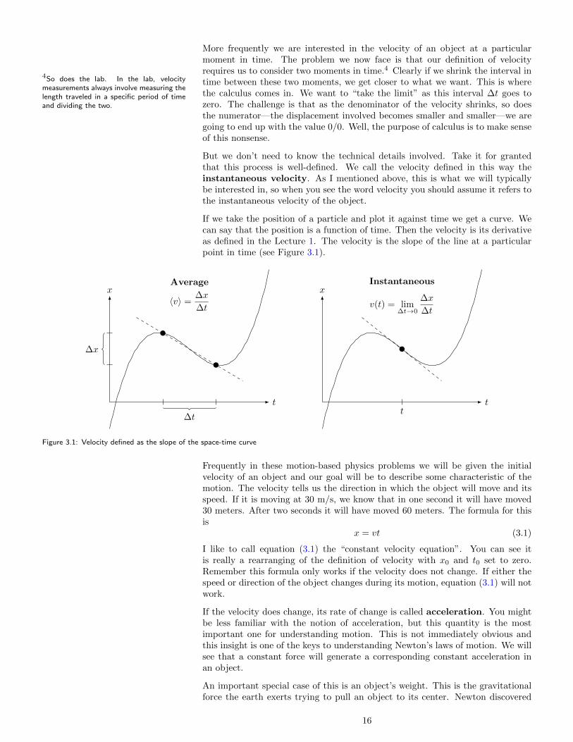
If we take the position of a particle and plot it against time we get a curve. Wecan say that the position is a function of time. Then the velocity is its derivativeas defined in the Lecture 1. The velocity is the slope of the line at a particularpoint in time (see Figure 3.1).

t

x

∆t

∆x

Average

〈v〉 =∆x

∆t

t

x

t

Instantaneous

v(t) = lim∆t→0

∆x

∆t

Figure 3.1: Velocity defined as the slope of the space-time curve

Frequently in these motion-based physics problems we will be given the initialvelocity of an object and our goal will be to describe some characteristic of themotion. The velocity tells us the direction in which the object will move and itsspeed. If it is moving at 30 m/s, we know that in one second it will have moved30 meters. After two seconds it will have moved 60 meters. The formula for thisis

x = vt (3.1)

I like to call equation (3.1) the “constant velocity equation”. You can see itis really a rearranging of the definition of velocity with x0 and t0 set to zero.Remember this formula only works if the velocity does not change. If either thespeed or direction of the object changes during its motion, equation (3.1) will notwork.

If the velocity does change, its rate of change is called acceleration. You mightbe less familiar with the notion of acceleration, but this quantity is the mostimportant one for understanding motion. This is not immediately obvious andthis insight is one of the keys to understanding Newton’s laws of motion. We willsee that a constant force will generate a corresponding constant acceleration inan object.

An important special case of this is an object’s weight. This is the gravitationalforce the earth exerts trying to pull an object to its center. Newton discovered

16

the laws that govern gravitation and was able to explain the workings of the solarsystem with it—we will talk about that in Lectures 4, 5, and 10. But on thesurface of the earth the force of gravity is fairly constant.5 Because of this, the

5Even in Newton’s time it was possible tomeasure the slight variations in the force ofgravity on the earth.

weight of an object causes it to fall with a constant acceleration of 9.8 meters persecond squared, symbolized by g.

So it is worth spending some time on understanding the motion of particles withconstant acceleration. Since the definition of acceleration parallels the definitionof velocity, we must have a formula that parallels equation (3.1). It is

v = v0 + at (3.2)

Remember that this formula depends upon the acceleration being constant—which is not always the case. We will see an example of that in Lecture 6 withuniform circular motion. In that case we need a different formula.

But how do we relate equation (3.2) to position? Calculus is designed to dealwith this type of problem—how do we calculate the position if the velocity ischanging? However, there is another trick we can use because the rate at whichthe velocity is changing is constant. If a quantity increases (or decreases) at aconstant rate, its average value is the average of the initial and final values.6 So,

6I won’t prove this statement, but considerthe following example. Take the series1,3,5,7,9,11. The average of these numbersis 6 which is also the average of the ends.Now take the series 2,4,8,16. The averageof these numbers is 7 1

2while the average of

the ends is 9.

〈v〉 = 12 (v + v0)

Now the average velocity by definition is the displacement divided by time, so wecan rewrite this as

x = 12 (v + v0)t (3.3)

By combining equations (3.2) and (3.3) we can derive three more equations:

x = v0t+ 12at

2 (3.4)

andx = vt− 1

2at2 (3.5)

andv2 = v2

0 + 2ax (3.6)

Equations (3.1)–(3.6) are the main results of this lecture. The rest of the lecturewill be about applying them.

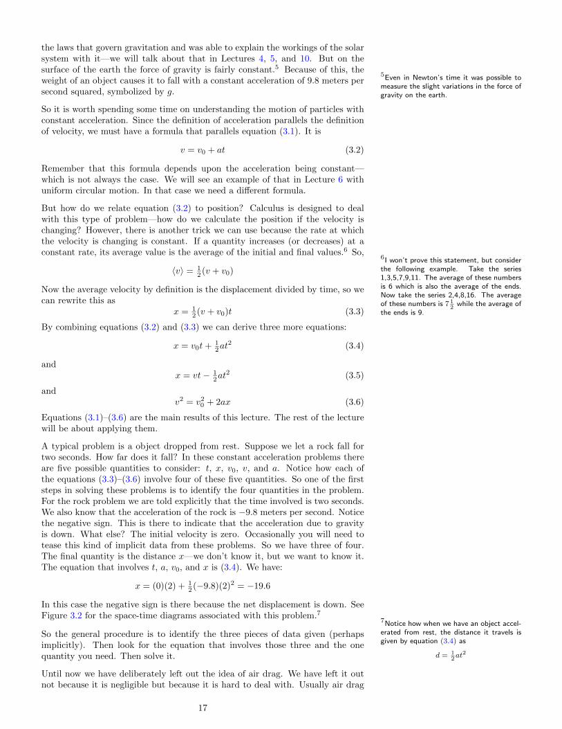
A typical problem is a object dropped from rest. Suppose we let a rock fall fortwo seconds. How far does it fall? In these constant acceleration problems thereare five possible quantities to consider: t, x, v0, v, and a. Notice how each ofthe equations (3.3)–(3.6) involve four of these five quantities. So one of the firststeps in solving these problems is to identify the four quantities in the problem.For the rock problem we are told explicitly that the time involved is two seconds.We also know that the acceleration of the rock is −9.8 meters per second. Noticethe negative sign. This is there to indicate that the acceleration due to gravityis down. What else? The initial velocity is zero. Occasionally you will need totease this kind of implicit data from these problems. So we have three of four.The final quantity is the distance x—we don’t know it, but we want to know it.The equation that involves t, a, v0, and x is (3.4). We have:

x = (0)(2) + 12 (−9.8)(2)2 = −19.6

In this case the negative sign is there because the net displacement is down. SeeFigure 3.2 for the space-time diagrams associated with this problem.7

7Notice how when we have an object accel-erated from rest, the distance it travels isgiven by equation (3.4) as

d = 12at2

So the general procedure is to identify the three pieces of data given (perhapsimplicitly). Then look for the equation that involves those three and the onequantity you need. Then solve it.

Until now we have deliberately left out the idea of air drag. We have left it outnot because it is negligible but because it is hard to deal with. Usually air drag

17

Figure 3.2: Space-time diagrams for free-fall with no air drag

t

a

0

−9.8

a = −9.8

t

v

0

v = −9.8t

t

x

0

x = −4.9t2

introduces a deceleration8 that is related to speed (the faster the speed, the larger

8When the acceleration opposes the di-rection of motion (or velocity) we call itdeceleration. Notice this is not the sameas negative acceleration which indicates itsdirection in space. When an object falls, thedeceleration from air drag points up.

the drag9). To solve these problems exactly requires some calculus. But we can

9This is why you can’t shoot fish in a barrel.The drag on the bullet is so great it canactually destroy the bullet itself. In fact,the higher caliber the more likely this willhappen.

get an approximate solution using a spreadsheet. The project for this term walksyou through how to do this. In fact, the spreadsheet approach will work even forthose problems when the calculus won’t.

Although the detail of free-fall with air drag are complicated, its final state iseasy enough to understand. Depending upon the details of the object and theair, a certain velocity will produce just enough drag to counter-balance the weightof the object. This is called the terminal velocity of the object. If the objectstarts with a velocity smaller than terminal (at rest, for example) then the netacceleration will increase the velocity. As the velocity increases, the drag willoppose more of the weight reducing the acceleration (slowing the rate at whichvelocity increases) until it reaches a steady-state at terminal velocity. See thespace-time graphs in Figure 3.3 and compare them with those in Figure 3.2.

Figure 3.3: Space-time diagrams for free-fall with air drag

t

a

0

a→ 0

t

v

0

v → vterminal

t

x

0

Until now we have only been discussing motion in one dimension. However, we canalso discuss the motion of a projectile flying under the influence of gravity withthese same equations. The problem of understanding the motion of projectilesgoes back to antiquity and wasn’t really solved until Galileo began to analyzethe idea of acceleration. His main insight is that the vertical component of themotion is under the constant acceleration (due to gravity) while the horizontalmotion has no acceleration—the horizontal motion obeys equation (3.1). Thismeans that the trajectory in space is a parabola.

For example, suppose we launch a projectile at a 60 angle with an initial speedof 45 meters per second. How far will it fly? Ignore air resistance. See Figure 3.4for reference.

The first step is to break the data into horizontal and vertical components. In thehorizontal we know that we will use equation (3.1) which involves x, v0x, and t.We are interested in solving for x and we are given enough information to solvefor v0x. This means we will be able to solve for t. This is common because theduration t is the same for the vertical and horizontal components. So the time isfrequently a problem solving “bridge” between the information contained in the

18

v0

θ = 60

R

Figure 3.4: Calculating the range of a projectile

horizontal and vertical components. In our case we need to calculate v0x first:

v0x = v0 cos θ = (45)(cos 60) = 22.500

But we can’t calculate the time because we don’t know the range. Since we haveexhausted the information contained in the horizontal motion, let’s turn to thevertical. We know v0y is given by:

v0x = v0 sin θ = (45)(sin 60) = 38.971

Of course, a = −9.8 since this is a free-fall problem (no air drag). We want todetermine t in order to use it in the horizontal calculation, so we need one morevertical quantity from the problem statement. The implicit data here is thaty = 0 because we are asked about the range—the distance the projectile travelsuntil it comes back to its original level. This is a net vertical displacement of zero.Given this information, we can use equation (3.4) to solve for t.

(0) = (38.971)(t) + 12 (−9.8)(t)2

=⇒ t = 7.9533

Since the duration of the vertical motion is the same as the horizontal, we canfinally solve for the total x-displacement. Thus,

x = (22.500)(7.9533) = 178.95

The original data was given with two significant digits, so we should round thisfinal answer to 180 meters.

It is sometimes convenient to know the range of a projectile without going throughthe logic of the previous example. We can summarize the results in the formula10

10You can derive this formula by simplyusing the same logic as our example problembut use letters without putting the numbersin. You’ll need to remember the trig identitysin 2θ = 2 sin θ cos θ.

R = (v20/g) sin 2θ (3.7)

This is called the range equation. Deriving formulas for every permutation ofthe projectile problem is tiresome, but this one can be useful on occasion.

There are a number of different of projectile questions that can be asked andsometimes finding the implicit data can get tricky. One trick in particular to noteis that at the top of the trajectory the vertical velocity vy is zero. Occasionallyyou’ll need to use the quadratic equation. But the principles you will need tosolve them are all laid out in this example.

Anyone who has played 30 seconds of golf will know that these problems arecompletely unrealistic and don’t represent the true motion of the ball. The airnot only resists the motion (air drag) but any spin on the ball will curve its pathas well. The dynamics of spin and its curving effect are extremely complicated11

11Ultimately it is based on Bernoulli’sprinciple—something we will talk about inLecture 14.

but if we focus our discussion on just the air drag, we can say a couple of things.

First, the range of the ball is much shorter than without drag. The longer thetime the ball is in the air the longer the effects of air resistance so the effectis most pronounced on projectiles with large initial velocities (there is also a

19

Figure 3.5: Projectile trajectory with heavy air drag

v0

θ

correspondingly larger air drag as well). It follows that the maximum height andthe time of flight are also shorter. See Figure 3.5

Second, notice how the angle with which the ball falls is nearly straight down.This is because the direction of the air drag is in the opposite direction of themotion. In the horizontal we have a deceleration without any correspondingacceleration. So the air drag slows down the horizontal motion. Of course itdoes the same to the vertical, but the vertical motion has gravity to help out.What happens is that the projectile basically stops its lateral motion and fallsdownward at a steeper angle than it goes up. Anyone who has played an outfieldposition in baseball can attest to the fact that catching a ball hit out that farusually involves looking nearly straight up to catch it.

This is the real motion of projectiles and is the main reason it was so difficultto determine the true motion of a projectile. In the Middle Ages it was thoughtthat a quantity called impetus was transferred to the object when it was thrown.After that, the motion was considered to be in a straight line as this impetus wasused up (kind of like a wind-up toy). After the impetus was exhausted, the objectwould fall straight down following a trajectory like a triangle. I like to call this a“cartoon trajectory” because this is how things work in the cartoons: the bad guyruns straight off the cliff for a while then, all of a sudden (usually with a puff ofsmoke), he falls straight down to his doom. The moral here is that there is moretruth to the cartoon trajectory than the clean parabolic motion the textbooksshow.

Next week we will introduce the key concept of force into our vocabulary. Beforewe dive into the deep end of Newton’s laws of motion we start by building someskills working with forces and vectors. We will learn the basic mechanical forces(weight, tension, support, and friction) and how they work. We will also learnwhat it means for these forces to be in equilibrium.

20

Lecture 4

Force and EquilibriumRead sections 4.6–4.11, sneak a peak at sections 10.1, 18.5, 21.2, andreview Lecture 2

When an object is subject to a force there are four physical quantities to dis-tinguish: the net force, torque, stress and pressure. Technically, pressure can beseen as a special case of stress, but we’ll set that consideration aside for now.

Force is the total amount of push or pull to which our object is subjected. Thepressure is the force divided by the area across which it is applied. This is whythe swami can lie of a bed of nails without getting hurt. The force of his weightis distributed, so that the pressure of support from any single nail is insufficientto pierce the skin. We won’t need the concept of pressure again until Lectures13 and 14. We will assume that any force is applied at a particular point on theobject. Just recognize that this is an approximation: every real force is appliedover a certain area.

Consider an object that is subject to a variety of forces all applied at differentpoints. Each of these forces will have a tendency to do three things: (1) push theobject in the direction of the force, (2) twist the object around its center of mass,and (3) deform the shape of the object.

If the direction of the force is precisely toward or away from the center of massthis force will not produce any kind of twisting or rotation. Otherwise the forceis said to produce torque which will be discussed in detail in Lecture 10.

An object is said to be in equilibrium when all the forces and torques balanceout. However, even if the object is in equilibrium it may still suffer deformationas a result of these forces. The amount of deformation is quantified by strainand the combination of forces causing this strain is called stress. We will talk abit about these concepts in Lecture 13 on elasticity. As you can guess, the detailscan get pretty hairy so we will only cover the high points.

For now we will ignore all of these issues. If we focus our attention on physicalsystems with negligible configuration (i.e., a particle) then there is no deformationto consider. In fact, the system has no extension, so the idea of torque doesn’teven apply. All we are left with is the simpler notion of force and its effects.

Obviously an object subject to a single force cannot be in equilibrium. We needtwo or more forces and they need to balance. Two forces must be equal andopposite in order to create equilibrium. In vector notation we may say:

~F1 + ~F2 = 0

Because of the way we have defined vectors in Lecture 2, this same formula works

21

for an arbitrary number of forces: ∑~Fi = 0

Here the summation is implied to run over all the values of i. If there are fourforces then the summation is a shorthand for

~F1 + ~F2 + ~F3 + ~F4 = 0

If necessary we may put a subscript on the summation symbol for clarity:∑i

~Fi = 0

or even more explicitly:4∑i=1

~Fi = 0

But I’ll usually be sloppy about this notation unless it is likely to cause confusion.

We walked through a typical force equilibrium problem in Lecture 2. It might beworth reviewing that example now (see page 11).

There are also different kinds of equilibrium: stable versus unstable. When forcesvary in time, the equilibrium they create may be destroyed. Typically the forces ina system depend upon its configuration (usually the distance between its parts).So, any motion in the system can change these forces. If these forces are suchthat any displacement tends to cause the system to return to equilibrium, this isstable equilibrium. A simple example is a marble in a bowl. If we displace themarble away from the center of the bowl it will be pushed back to center. Turn thebowl upside-down and you have unstable equilibrium. A pencil standing on it’spoint is another example. You may have seen a person holding a broom upside-down with the palm of their hand. This is an example of dynamic equilibrium.In this case the forces are not dependent on the configuration but on a feedbackloop (i.e., the person doing the balancing). Dynamic equilibrium is often usedto combat unstable equilibrium, but if one is not careful it can lead to literallyexplosive results.

For now we only consider forces that are constant. So if they are in equilibriumthey will remain that way.

There is one other point to make regarding equilibrium. No net force on aobject does not imply that the object is stationary. What it implies is thatthe acceleration is zero—the object may be moving with constant velocity. Wesaw an example of this with air drag and terminal velocity in Lecture 3. Althoughit is not common to make this distinction, it may be worth calling equilibrium ona moving object kinetic equilibrium as opposed to static equilibrium for anobject at rest.

In our inventory of mechanical forces to consider, the simplest is weight.1 In1Our book discusses weight in the contextof the Newton’s law of gravity (section 4.7).I prefer to wait and talk about the law ofgravity in Lecture 6.

the English system of units the pound is a primary unit. However, the influenceof gravity can vary slightly depending on where you are on the surface of theplanet. This means that the weight will vary as well. In the metric system, massis primary and weight is secondary. Mass is a difficult quantity to define preciselywithout using Newton’s laws (to be discussed in the next lecture). However, theweight of an object is simply related to its mass via

W = mg

If the gravitational acceleration increases slightly so does the weight. The SI unitfor weight is called the newton and the metric unit for mass is the kilogram.Under standard earth gravity, a one kilogram mass will weigh about 9.8 newtonswhich is equivalent to about 2.2 pounds.

22

Tension will come up again when we discuss elasticity in Lecture 13, but for nowwe only consider it in the context of an ideal string. A string is ideal if it hasnegligible weight and does not stretch at all. A string like this essentially transmitsthe force from one end to the other. Combine this with an ideal pulley (friction-less, negligible mass) and you can create a block-and-tackle. Take for exampleFigure 4.1. Notice how the larger weight is supported by two strings. But thetwo strings are really the same string, so the force that supports the weight isactually the tension multiplied by two. The tension is in balance with the smallerweight. This block-and-tackle system essentially multiplies force by two. Thisis called the mechanical advantage of the system. Actually, this is the idealmechanical advantage. The true mechanical advantage will take into account thefriction and the masses of the pulleys and strings. In fact, the ratio of actual toideal mechanical advantage is called the efficiency of this simple machine.

Figure 4.1: Simple block and tackle withmechanical advantage of two

The third mechanical force we will consider is a support force. Put a 10 kilogrammass on the table. The table supports this mass by holding it up against itsweight. This force of support is ultimately from elastic forces: the weight actuallydeforms the surface of the table slightly. The table resists this deformation with asupport force. Understanding this is important because there is no “formula” thatgoverns the support force—it is a reaction to the other forces in the problem. Themagnitude of the support is simply that which is required to balance the forcesagainst it.

These forces are sometimes called constraint forces because the surface thatprovides the support constrains the motion of the object. The motion can onlyoccur parallel to the surface because the force resists any motion into the surface.I prefer to call them support forces because that seems to me to describe thembest. However, it is much more common to call these normal forces. The reasonfor this is that in mathematical jargon the word “normal” means perpendicularand these forces always operate perpendicular to the surface doing the supporting.

A more involved example of the use of support forces in a problem is a weightsupported by an inclined plane. Review Figure 4.2. Because the support isperpendicular to the slope of the plane, only a component is available to counter-balance the weight. The remaining component wants to push the block down theslope. However, the tension in the string tied to the smaller mass holds it back.This tension is coming from the weight of the smaller mass pulling down acrossthe pulley. If the masses are in the right combination, these forces will balancein equilibrium. 30

Weight

Tension

Support

Figure 4.2: Inclined plane with pulleyI have redrawn these three forces in Figure 4.3. When we collect all the forcesacting on one part of the system, it is called a free-body diagram. It isalmost always best to align your coordinate system with any forces of constraint.Usually the constraints are the most difficult forces to calculate in a problem.By properly orienting the coordinates we can usually begin the calculation in thedimension perpendicular to the constraint to get more information before tacklingthe constraint itself. In fact, it is sometimes possible to solve a problem withouteven solving for the constraint.

In this case it is pretty simple. Notice how the components of the weight corre-spond exactly with the tension and support forces. This shows that the massesare in equilibrium.

x

y

Weight

Tension

Support

Figure 4.3: Free-body diagram from Figure4.2 (magnified 2x)

If we call the larger mass #2, the component of its weight that points down theplane to the left is given by

W2 sin 30 = 0.500W2

This must equal the tension in the rope and that tension equals the weight ofthe smaller mass (which we will call #1). We have 0.500W2 = W1. The ideal

23

mechanical advantage of this inclined plane is two. This can be seen by

MA = W2/W1 = 2

In general, the ideal mechanical advantage of the inclined place is given by 1/ sin θ.

The fourth mechanical force to consider is friction which occurs whenever twosurfaces are in contact. The amount of friction depends on two factors: (1) theamount of support force that is pressing them together, and (2) the nature ofthe two surfaces in contact. The effect of the second factor is captured in thecoefficient of friction and is given the symbol µ. Its value is between 0 and 1.The formula for friction is2

2This is our first example of an constitutiveequation. I mentioned in the first lectureabout how one of the roles of the deductiveapproach is to explain from first principlesthe values obtained for equalities such asthese. This one, however, is nearly im-possible and is dependent on a variety offactors. As such, these numbers for variouscombinations of surfaces can only be derivedon average from the lab.

F = µN

Now, there are two varieties of friction: static and kinetic. If the block is sliding,kinetic friction applies and the force is given by Fk = µkN where µk is thecoefficient of kinetic friction. Remember that the forces on a moving object maystill be in equilibrium (previously we called this kinetic equilibrium). You mayencounter a homework problem or two where an object is sliding at constantspeed. In that case, you know two things: (1) the friction is kinetic and (2) theforces all balance.

If the block is not sliding, then clearly the forces are in static equilibrium. In thiscase the static friction is whatever it needs to be to maintain balance—just likethe support forces we studied earlier. However, the static friction has a maximumvalue. If the force required to maintain balance exceeds this maximum value, theblock won’t be able to resist moving. Thus, if the block is stationary we knowthe static friction is less than this maximum value. This upper bound is givenby the formula Fs ≤ µsN , where µs is the coefficient of static friction—a numbergreater than its kinetic cousin.

As an example, consider Figure 4.4, which is essentially the same as Figure 4.2with the tension replaced by friction. We will assume that this object is inequilibrium, so the free body diagram is essentially the same as Figure 4.3.30

Weight

Friction

Support

Figure 4.4: Inclined plane with friction Therefore the magnitude of the normal support force is equal to

W cos 30 = 0.866W

and the magnitude of the friction force is equal to

W sin 30 = 0.500W

Since the static friction force is related to the support force according to Fs ≤µsN , we have a constraint placed upon the coefficient µs:

µs ≥ 0.577

In other words, if the coefficient of static friction is less than 0.577 (in general,1/ tan θ), the block will slide because there won’t be enough static friction to holdit in place.

This is the last constant mechanical force for us to consider. However, we willsee more forces in the upcoming lectures. For example, in Lecture 13 we willdiscover the formula for elastic forces. Truly, elastic forces are the cause of bothtension and support, but in that lecture we will focus on the role of deformationin elasticity which we are neglecting here.

All of these forces that I’ve classified as “mechanical” (including elastic forces)require the objects to be in contact. In contrast, gravity and the electromagneticforces are long-range forces which act at a distance. We will talk about theelectric and magnetic forces in Lectures 23 and 24, respectively. The law for theelectric force is quite similar to Newton’s law of gravity which we will study in

24

Lecture 6. The magnetic force is unique in that it causes a deflection that isperpendicular to the motion of the particle. Using results from Lecture 6 wewill see that this produces a characteristic spiral motion. This perpendiculardeflection is also a characteristic of the Coriolis force we will mention in Lecture9.3

3There is a peculiar fascination with thedistinction between contact forces and long-range forces in the history of physics. Thelong-range nature of gravity really buggedNewton: he called it “occultish”. Prior toNewton, it was felt that any force had tobe a contact force: for example, Descartesfilled the solar system with a fluid that keptthe planets in motion. As a consequenceof the study of electromagnetism in the19th century, a kind of middle ground wasestablished: the force field. We say thatspace is filled with gravitational and electro-magnetic fields which operate as media forthe transmission of these forces. But thefield is not mechanical—they obey laws oftheir own independent of mechanics. How-ever, the modern development of quantumfield theory has written a new chapter inthe debate between long-range and contactforces which comes nearly full circle.

In Lectures 29 and 30 we will also encounter the existence of two nuclear forces.This is really a misnomer though because at that level we cannot avoid usingquantum mechanics and the idea of force must be replaced with the more generalnotion of “interaction”. We will lay the ground work for moving beyond force inLectures 7 and 8 when we talk about energy and momentum.

Next week we will introduce Newton’s three laws of motion. The first law willcause us to consider reference frames in motion. We will find that if we are notcareful choosing these frames we may introduce “fictitious forces” into the laws ofmotion. We will also see where Einstein’s relativity touches the laws of motion.Newton’s second law establishes the connection between force and accelerationalluded to in Lecture 3. Finally, the third law will introduce us to systems andthe role of internal and external forces.

25

26

Lecture 5

Newton’s Laws of MotionRead sections 4.1–4.5 and 4.11, sneak a peak at sections 28.1–28.2

Inertia is the property of a system to maintain its state of motion. When anobject is moving it has a tendency to keep moving. This is why you never wantto stand in front of a moving train. This principle of inertia may seem obviousbut it has not always been that way. The critical modern insight is to set asidethe realities of friction and weight. Without this conceptual distinction, Aristotletaught that every object has its place. In other words, objects have an intrinsictendency based on their composition to move until they come to rest in theirplace. Things made of earth fall down, things made of air float up.

Galileo was the first person to apply the idea of inertia to objects in motion in aquantitative way. He was able to see the central point that once an object is setin motion the only reason it stops is friction and that friction is external to theobject. Whether it is dragging against air resistance or dragging across a surface,if this friction is eliminated there is nothing to stop the motion. In situationswhere the effect of friction is minimized (an icy road, a rolling ball) this inertiais more obvious.

This principle of inertia is quantified in the notion of mass. If an object is inmotion, the larger mass is harder to stop. This works in reverse too: the moremassive an object, the more difficult it is to push it into motion. If we decide ona particular object as our unit of mass we can measure the force required to get itto move at a particular rate. If twice the force is required to get a second objectto move at the same rate, we say it has twice the mass. So mass measures theamount of resistance an object will have to changing its state of motion.

Newton’s first law of motion is Galileo’s principle of inertia. Newton’s wordingis as follows:

Every body perseveres in its state of rest, or of uniform motion ina right line, unless it is compelled to change that state by forcesimpressed thereon.

When first exposed to this idea it is easy to associate it with something likepushing a box across the floor: when you start out, with just a small amount offorce, the box does not move at all. Only after a certain critical level of pushinghas been reached will the box move. This is not inertia. This is friction. It isbetter to think of the force required to stop an object in motion—this is tied tothe idea of inertia more directly than considering the force required to start themotion.

Galileo also recognized something we now call the principle of relativity.11Not the theory of relativity—that wasEinstein. See Lecture 26.

27

Imagine you are watching boats sail across a calm lake. There is a man hangingoff the mast of a ship making repairs. The wrench he is holding slips and drops 30feet straight down striking the base of the mast (we are going to ignore air drag).Since the wrench has a bright orange handle you see it clearly tumble down asthe ship drifts across your field of view. But from your viewpoint, the path ofthe wrench is not straight but a parabola. Of course you agree that the wrenchstrikes the base of the mast, but to you the ship just happens to catch it on itsway down.

Well, “just happens” is an overstatement because the reason the wrench is notfalling straight down is that before it was dropped, it was moving with the driftvelocity of the ship. The wrench continues to drift with this velocity while itundergoes acceleration downward due to gravity.

Here’s the point: is the ship moving? Yes, you say, of course it is moving: itis drifting across the lake. What does the repairman say? Yes, he says, I canlook out at the shore and see the ship is moving. Fine: everyone agrees. Later,below deck, he is eating lunch and drops his fork. The fork falls straight downlike the wrench—is the ship moving? Yes, but without a reference frame tied toshore, the repairman cannot tell. All motion is always measured relative to somereference frame. And this is the principle of relativity: within a reference framemoving with constant velocity, it is not possible to determine this drift velocitybased on the relative observations made within that frame. The laws of physicsare independent of the velocity of the frame.

This abstract symmetry is broken by the fact that we live on earth. There is adistinct up-and-down direction due to gravity and a distinct state of rest due tofriction and air drag. But take away gravity and friction and you have this kindof free-fall world where the principle of relativity rules.2

2This is one of the reasons why a pool tableis such a good place to learn physics. Thehorizontal nature of the table eliminates theeffect of gravity and the balls roll so theeffects of friction are minimized.

There is a positive way to state the principle of relativity, too. Since the lawsof physics work in any frame (moving with constant velocity), you are free tochoose whichever you like as your rest frame. In fact, in order to do any kind ofcalculating, you must start by choosing this frame. The point is that the choiceis arbitrary—there is no “natural” choice.

But not completely arbitrary. It may seem like the airplane is at rest when youare at cruising speed, but hit some turbulence and you’re not at rest any more.The key is that the frame must move with constant velocity: no acceleration. Areference frame in which Newton’s first law holds is called an inertial frame.Non-inertial frames like a car making a turn will have pushes and pulls which aredue to the non-constant velocity (either speed or direction) of the frame. We useNewton’s first law to identify an inertial frame. The principle of relativity impliesthat any frame moving relative to another inertial frame with constant velocityis also inertial.

Newton’s second law of motion presumes we are working in an inertial framedefined by the first law. According to Newton we have:

The alteration of motion is ever proportional to the motive forceimpressed; and is made in the direction of the right line in whichthat force is impressed.

This is commonly written as~F = m~a (5.1)

This formulation is due to Euler.3 Notice how neither acceleration nor mass are3Euler’s contributions to both mathematicsand physics are extensive. In a sense Eulercompleted Newton’s laws by extending themto rigid objects—cf. Lectures 9 and 10.

mentioned in Newton’s formulation. He uses the phrase “alteration of motion”which may seem vague, but earlier he defined this “quantity of motion” as:

The quantity of motion is the measure of the same, arising from thevelocity and quantity of matter conjointly.

28

Today we use the term mass for “quantity of matter” and the “quantity of motion”we call momentum (see Lecture 8). In other words, Newton’s second law asoriginally formulated states that force changes momentum. Now if the mass ofthe object is constant, the part of the momentum that changes is the velocity, sothis is equivalent to Euler’s formulation. But if the mass is not constant (a rocketship is a good example) the more general law based on momentum is needed.

Unless otherwise stated, assume the mass is constant and use equation (5.1).

If an object is under the influence of several forces, we need to calculate thevector sum of these forces to determine the direction of acceleration. Clearlythe object can only move in one direction, so we need one net force vector toput on the left side of the second law. This is often the most difficult part insolving these problems: identifying the forces and adding them up to some netforce. Of course, the forces may all balance. In this case the vector sum is zero.Accordingly equation (5.1) implies ~a = 0, so the object in equilibrium will eithermove with constant velocity or remain at rest. You can see how the problemsfrom the previous lecture are now a special case of the more general second law.

Another way to express Newton’s second law is that any unbalanced force willproduce acceleration. This emphasizes the initial step of calculating the net forceon an object. A classic example problem is the Atwood machine which is simplytwo weights hanging over a pulley (see Figure 5.1). Just by looking at the diagramyou can see what will happen: the larger weight will drop but slower than normalbecause it will have to pull the smaller weight up. We now need to calculate theresult.

aa

Figure 5.1: Atwood machineOne important thing to realize here is that this is a system with two parts (threeif you count the string). Each weight has a different net force acting on it andeach weight corresponds to an application of equation (5.1). Let’s call the mass ofthe smaller weight m and the mass of the larger weight M . Therefore the weightof each is mg and Mg respectively.

The force that opposes the weight of each is the tension in the string, whichwe will label T and it is equal on both sides. But recognize that the tension isundetermined—it is equal to neither the smaller nor larger weight. This is aneasy mistake to make. I think this is because we draw the diagram and forgetthat it represents a snapshot in time—the objects are actually moving and theforces are out of balance. I try to draw a little arrow with an a to remind myselfthe objects are accelerating.

So, we are ready to apply Newton’s second law. This problem is simple so we willjump the result. We’ll walk a bit more slowly in the next problem to show all thesteps. From the smallest weight we have:

T −mg = ma

and from the larger weight we have:

T −Mg = −Ma

Notice the signs. You must be deliberate with the signs because these quantitiesare vectors. In both cases the tension from the string pulls up, so they get positivesigns. Similarly the weights pull down, so they get negative signs. The smallerblock will accelerate up so it is positive, and the larger block will accelerate downso it is negative. The magnitude of the acceleration of the two blocks are thesame because they are tied together.

From a mathematical standpoint we have two equations with two unknowns (Tand a). This means we can solve for both. In order to solve for the accelerationwe will use the first equation to eliminate the T from the second. This yields

(ma+mg)−Mg = −Ma

29

Solving for a gives

a =M −mM +m

g

It is sometimes helpful to look at some extreme cases as a double check. If m = M ,then we have a = 0 which makes sense—the weights balance. If m = 0 then a = gwhich also makes sense because if there is no smaller weight the larger will simplyfall under the influence of gravity. Intermediate cases are in between, so thisanswer checks out.

Now for a more complicated example. Examine the situation in Figure 5.2. Thisis similar to Figure 4.2, but the hanging weight is smaller (and the tension is less)so the larger mass will slide to the left. Suppose the larger mass is 10 kilogramsand the smaller mass is 3 kilograms. How long will it take the block to slidedown the incline from rest if the plane is one meter long? What will be its finalvelocity?30

aa

Weight

Tension

Support

Figure 5.2: Inclined slide with pulley The first step in any of these problems is to draw a good free-body diagram foreach piece of the system. Fortunately for me we have already done this in theLecture 4 (see page 23) except that the tension is a bit smaller now. In thisproblem the tension is not equal to the smaller weight because the forces are notin balance. In fact we know that the tension is larger than the smaller weightbecause it will need to lift the smaller weight up as the larger mass slides downthe incline. The situation on this smaller mass is similar to the previous example,so we have

T −mg = ma

just as before. This gives us a formula for tension, T = m(a + g), which we canuse in the analysis of the motion of the larger mass.

Looking back at the free body diagram in Figure 4.2, we can see that the tensionopposes the x-component of the weight. We know that these will not balance,but we can still use Newton’s second law. In this case, the weight is 98 newtons.The x-component of the weight in this inclined coordinate system is

Wx = (98)(cos 240) = −49

The 240 is measured from the positive x-direction. The sign of this component isnegative because it points to the left. Notice how the positive x-direction for ourcoordinate system is pointing up the incline. This also means we should expectthe acceleration of the larger block to be negative.

So, from the x-component of the larger mass we have

−49 + (3)(a+ 9.8) = (10)(−a)

which we can solve for a. Thus,

a = 1.5077

We have not yet answered the question, however. We were asked about time andfinal velocity. We were given the initial velocity (“at rest”) and the displacement,so we should consider using equation (3.4) to get the time. Thus,

(−1) = (0)(t) + 12 (−1.5077)(t)2

The negative signs are there because the motion is to the left. The final answeris 1.15 seconds. In order to determine the final velocity, we use equation (3.6).Solving yields 1.74 meters per second.

The various combination of possible problems are endless. Add friction into themix and you have a really hard problem. But in each case the procedure is thesame. Focus first on getting the acceleration of the objects by applying Newton’ssecond law. Thus,

30

1. Identify all the forces in play.

2. Draw a free-body diagram for each part of the system (remember to alignyour coordinates along any natural constraint).

3. Determine the components of the net force in each diagram.

Each part and each dimension will yield an equation via Newton’s second law.Sometimes you won’t need all of these equations but they are all valid. Once youhave the formulas, calculate the acceleration of the objects.4 From there use the

4If the system has multiple parts usually theaccelerations are the same, but sometimesnot—the parts of a block and tackle systemswill not have the same acceleration, forexample.

techniques from Lecture 3 to answer the specific question.

So far we have used Newton’s law to calculate acceleration given a certain setof forces. The process can work the other way too. We can investigate thecharacter of a force from the acceleration it causes on the objects it influences.For example, we can do experiments with static electricity do determine the waythat the electric force is dependent upon distance.

One interesting example of using the second law this way is in dealing withinertial forces. I have said before how the second law is only valid in an inertialframe. So a particle free from the influence of outside forces will move in astraight line at constant speed. If we are in a non-inertial frame, the frame willmove underneath the force-free particle. From the point of view of someone tiedto the frame, the particle will experience an acceleration. Being a good studentof Newton, this person would be led to postulate the existence of some force thatcauses this acceleration. However, this force is not due to outside forces but is anartifact of the non-inertial frame. This is why these kind of “forces” are calledfictitious forces.

The most common example of such is the centrifugal force. If you stand ona merry-go-round you will feel a force that wants to fling you off—out fromthe center of rotation. Your inertia is propelling you in a straight line which,relative to the rotating merry-go-round, is out. You must overcome your inertia bypushing in to stay on the rotating frame. You interpret this as counter-balancingsome centrifugal force. But this centrifugal force has no source: no object ispulling you out. It is merely a manifestation of the principle of inertia.

These inertial forces are always proportional to the mass of the object. This isbecause they are enforcing the principle of inertia. The greater the mass of anobject, the larger its inertia. These forces always take the form ma from equation(5.1), so that the resulting acceleration is independent of the object. This isbecause the acceleration is due to the nature of frame rather than the object.Another way to recognize an inertial force is that it will disappear if the rightframe of reference is chosen. These frames are precisely the inertial frames wetalked about earlier.

Notice that gravity has these same qualities. We infer the force of gravity fromthe acceleration we see in falling objects. This acceleration is independent of theobject. The force of weight is given by the formula mg. The fact that the masswhich appears in the weight formula is the same as the inertia that appears inNewton’s second law is called the equivalence principle. When Einstein wentlooking for a place to rebuild a new theory of gravity consistent with relativity,he started with this principle. He imagined a physicist in a falling elevator. Inthis frame, gravity would appear to be turned off. Therefore, a reference frameaccelerating in free-fall is actually an inertial frame of reference. This thoughtexperiment only works for a small space (for instance, you can’t find a frame thatwill “turn off” gravity for the whole planet), but that was enough of a startingpoint to build the general theory of relativity.

Newton’s third law of motion is often a bit confusing because the context isdifferent than the first two. In the first two laws we deal with a single particle.Even when we used the second law to analyze a system, the second law only applies

31

for one part at a time. The third law deals with pairs of particles. Newton sez. . .

To every action there is always opposed an equal reaction: or themutual actions of two bodies upon each other are always equal, anddirected to contrary parts.

Until now we have discussed forces that come from outside. Now we talk aboutforces internal to the system of particles—forces of interaction. The third law istelling us that every interaction in nature involves an equal and opposite pair offorces. It is a statement about the nature of force itself.

In practice, the third law is not very helpful. It’s one of those things that makethe whole conceptual structure work, but the hard work is done by the secondlaw. It does imply something that is very important however. Since every forcechanges momentum and every interaction involves equal and opposite forces, everyinteraction involves equal and opposite changes in momentum. In other words, wecan conceive of the interaction as consisting in the exchange of momentum. Thisviewpoint forms a perfect compliment to the idea of energy and we will explorethis perspective more in Lectures 7 and 8.5

5It is also a key element of quantum fieldtheory—see Lecture 27. But for now we will stick with Newton’s laws for a bit. Next week we will explore

our first non-constant force: the force required to maintain circular motion. Wewill talk a bit about circles and the velocity and acceleration involved in circularmotion. This will lead into the idea of centripetal force. We will discover thatthe force of gravity which holds the planets in place is also centripetal. Newton’slaw of gravity will be introduced and we do some prep work for the Lecture 11on celestial mechanics.

32

Lecture 6

Circular Motion and GravityRead sections 5.1–5.5, review section 4.7, and sneak a peak at sections10.1–10.2

The ancient Greeks had a love affair with circles and spheres. These are the onlyshapes that can change without changing. Looking out at the night sky, theyimagined astronomically large transparent spheres spinning around the earth. Ineach was lodged a planet which rotated with them like a embedded jewel.

Though we no longer think that way about the night skies, there is still somethingmagical about the circle. We can talk about the paradoxical ratio π, the compli-cations of abstract geometry, or complex numbers—behind every cycle in natureis a circle waiting to be found. We will exploit this fact in Lecture 12 when wetalk about simple harmonic motion. But for now we will talk about some basics.

The most important point of the circle is not on the circle: its center. Thecircumference is related to the radius of the circle by C = 2πr. So the averagespeed of an object rotating in a circle is given by v = 2πr/T where T representsthe amount of time required to complete one cycle which we call its period. Wewill call the motion uniform circular motion if the speed has this average valuethe whole time.

We will normally talk about uniform circular motion in the context of a fullcircle, but it does not have to be that way. A car making a right turn can movewith uniform circular motion for a quarter of a circle. The results from thislecture will be applicable to that motion as well. Whenever a path is curved thatcurvature can be characterized by a circle with the same curvature. Since thecircle is characterized by its radius, we can quantify this curvature by its radiusof curvature. The smaller the radius of curvature, the tighter the curvature ofthe path.1

1In fact, the curvature is related to thereciprocal of the second derivative of thepath. One way to see this is that the firstderivative is related to the slope or directionof the path. The second derivative willquantify how much this slope or directionchanges.

We know from the principle of inertia that circular motion cannot be maintainedwithout a force. It would be helpful to know what acceleration is required tomaintain a particular state of uniform circular motion. The formula

a = v2/r (6.1)

can be derived by comparing the velocity vectors at two different points in themotion. See Figure 6.1. By definition, the acceleration is the difference betweenthese two velocity vectors divided by the time it takes to get between them.These three vectors form a triangle. In the meantime, the radius vector thatsweeps from one point to the other also forms a triangle. The other side of thistriangle is almost the same as the arc-length of the circle traveled.2 These two

2This approximation becomes better thesmaller the duration involved.

triangles are similar, so the ratio of the sides are equal. In particular

at

v=vt

r

33

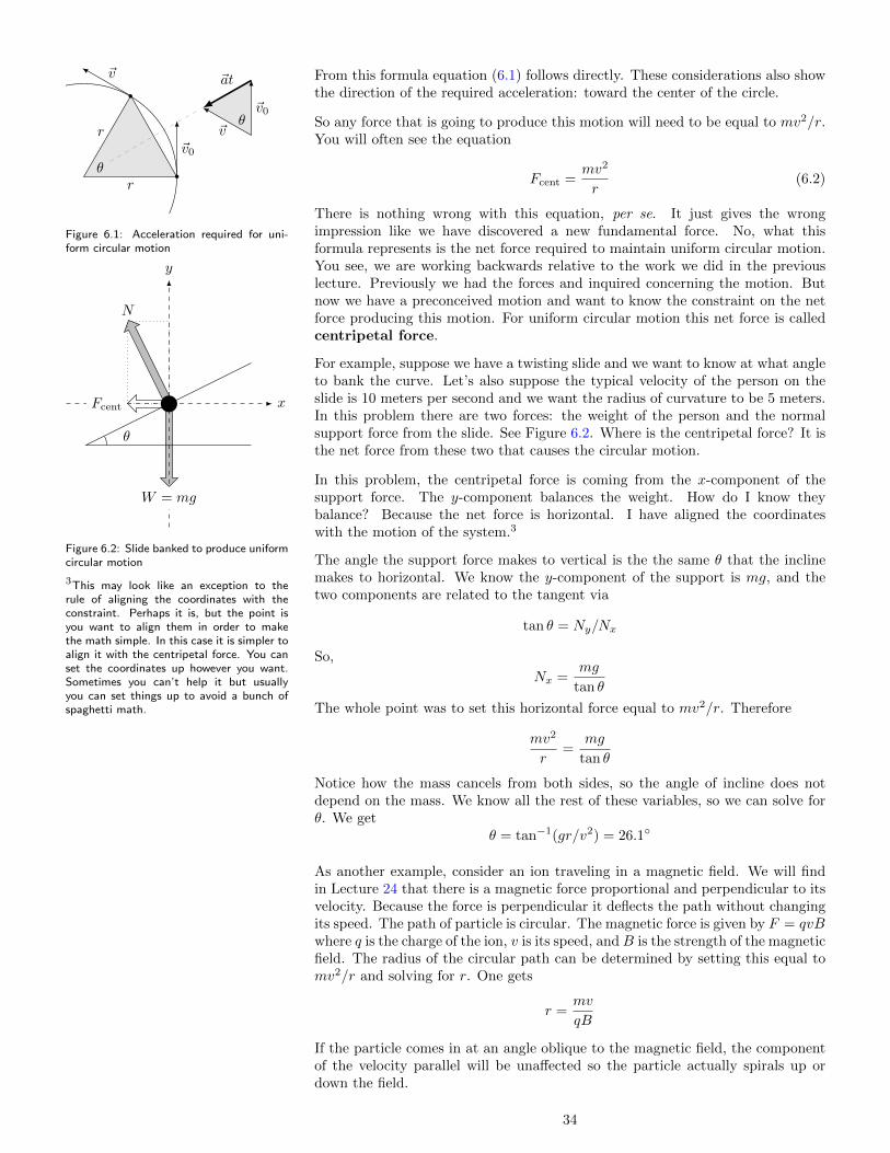
From this formula equation (6.1) follows directly. These considerations also showthe direction of the required acceleration: toward the center of the circle.

r

~v0

r

~v

θ

~v0

~v

~at

θ

~v = ~v0 + ~at

Figure 6.1: Acceleration required for uni-form circular motion

So any force that is going to produce this motion will need to be equal to mv2/r.You will often see the equation

Fcent =mv2

r(6.2)

There is nothing wrong with this equation, per se. It just gives the wrongimpression like we have discovered a new fundamental force. No, what thisformula represents is the net force required to maintain uniform circular motion.You see, we are working backwards relative to the work we did in the previouslecture. Previously we had the forces and inquired concerning the motion. Butnow we have a preconceived motion and want to know the constraint on the netforce producing this motion. For uniform circular motion this net force is calledcentripetal force.

For example, suppose we have a twisting slide and we want to know at what angleto bank the curve. Let’s also suppose the typical velocity of the person on theslide is 10 meters per second and we want the radius of curvature to be 5 meters.In this problem there are two forces: the weight of the person and the normalsupport force from the slide. See Figure 6.2. Where is the centripetal force? It isthe net force from these two that causes the circular motion.

x

y

θ

W = mg

N

Fcent

Figure 6.2: Slide banked to produce uniformcircular motion

In this problem, the centripetal force is coming from the x-component of thesupport force. The y-component balances the weight. How do I know theybalance? Because the net force is horizontal. I have aligned the coordinateswith the motion of the system.3

3This may look like an exception to therule of aligning the coordinates with theconstraint. Perhaps it is, but the point isyou want to align them in order to makethe math simple. In this case it is simpler toalign it with the centripetal force. You canset the coordinates up however you want.Sometimes you can’t help it but usuallyyou can set things up to avoid a bunch ofspaghetti math.

The angle the support force makes to vertical is the the same θ that the inclinemakes to horizontal. We know the y-component of the support is mg, and thetwo components are related to the tangent via

tan θ = Ny/Nx

So,

Nx =mg

tan θ

The whole point was to set this horizontal force equal to mv2/r. Therefore

mv2

r=

mg

tan θ

Notice how the mass cancels from both sides, so the angle of incline does notdepend on the mass. We know all the rest of these variables, so we can solve forθ. We get

θ = tan−1(gr/v2) = 26.1

As another example, consider an ion traveling in a magnetic field. We will findin Lecture 24 that there is a magnetic force proportional and perpendicular to itsvelocity. Because the force is perpendicular it deflects the path without changingits speed. The path of particle is circular. The magnetic force is given by F = qvBwhere q is the charge of the ion, v is its speed, andB is the strength of the magneticfield. The radius of the circular path can be determined by setting this equal tomv2/r and solving for r. One gets

r =mv

qB

If the particle comes in at an angle oblique to the magnetic field, the componentof the velocity parallel will be unaffected so the particle actually spirals up ordown the field.

34

This happens in the earth’s magnetic field. The solar wind is composed of ionsof hydrogen. When they enter the earth’s magnetic field they begin a spiralingmotion and are funneled along the magnetic field lines. As they get closer tothe poles, the magnetic field becomes more dense and the radius of the spiraldecreases. The collision of these particles with the atmosphere causes the AuroraBorealis, more commonly known as the northern lights.

We know that every particle in uniform circular motion does so because it isunder the influence of a centripetal force of some sort. This also applies to thesolar system. Now, even to the ancient Greeks it was known that the planets donot orbit around the sun in a perfect circle.4 But once the transparent spheres

4Mercury and Mars have the least circularorbits of the eight planets in the solarsystem.

were definitively shattered by Galileo, the nature of the centripetal force holdingthe planets in place came into question. By Newton’s time it was a commonassumption that this force obeyed an inverse-square law. That is, the force ofgravity between two objects is inversely proportional to the distance betweenthem. What Newton did was to prove it.

The application of Newton’s laws of motion to the motion of the the planetsdominates the Principia. Along with his three laws of motion, he lays out theuniversal law of gravity as

F =GMm

r2(6.3)

We will limit ourselves to the special case when M m though Newton himselfdid not. This means that the larger mass M is basically unaffected by the motionof the smaller mass m. The value of G is a universal constant characterizing theforce of gravity. In SI units it has a value of 6.673× 10−11.

For Newton the force of gravity was the archetypal centripetal force. However,for him the term meant something different than it does for us. We reserve thenotion of centripetal force for that associated with circular motion. For Newtona centripetal force was any force whose direction was always toward a particularpoint in space. Today we would use the term a central force to describe such athing. So we say that gravity is a central force.

For any central force it makes sense to describe motion in terms of polar co-ordinates. In polar coordinates we describe the location of an object by itsdistance from a particular point in space and its angle from a particular line fromthat point. This is an example of a non-Cartesian coordinate system that can behelpful in the analysis of orbital mechanics. Compare the systems in Figure 6.3.We will mention this again in the Lecture 11.

x

y

r

θ

Figure 6.3: Cartesian versus polar coordi-nates

A generation before Newton, Kepler had painstakingly examined the best knownastronomical data of his day (mostly from the study of the motion of Mars). Hewas able to distill their pattern into what is now known as Kepler’s three lawsof planetary motion. They are:

1. The orbit of the planets are elliptical with the sun located at one of the foci.

2. The rate of area swept out by the line from the sun to the planet is constant.

3. The square of the orbital period is proportional to the cube of the radius ofthe orbit.

It is easy to show that Kepler’s third law is a consequence of the law of gravityby simply setting the inverse-square law equal to mv2/r. Thus,

GMm

r2=mv2

r=⇒ GM = rv2

But the orbital period is related to the velocity by v = 2πr/T , so we have

GMT 2 = 4π2r3 (6.4)

35

This is Kepler’s third law.5 Newton was also able to show that the other two laws5In 1934 the analysis of the rate at galaxiesspin was determined to violate Kepler’sthird law. The speed of the stars onthe outer edges is much too fast. Thisimplies that there is a lot more mass in thegalaxies holding them together than can beinferred from the stars we see. This andother astronomical observations lead manyto postulate the existence of dark matterin the universe (another way of dealing withthe problem is to assert that the inverse-square law of gravity does not hold for theseextreme distances). It’s a bit embarrassingto admit that we have no clue about thecomposition of approximately 80% of theknown universe. See here for more info.

followed from the law of gravity, but those proofs are a bit more complicated.6

6In Lecture 11 we will see how the secondlaw follows from the central nature of theforce of gravity

Another example of the use of these formulas is in calculating geostationaryorbit. This the distance in which a satellite will have an orbital period of exactlyone day. This means that the satellite will simply remain overhead and is usefulfor communication satellites. Since there are 86,400 seconds in a day, we cancalculate this orbit distance using Kepler’s third law. For the earth we haveGM = 3.99× 1014, so

r = 4.22× 107

or 42,200 kilometers from the center of the earth. This corresponds to an altitudeof 35,800 kilometers above sea level. GPS satellites orbit at an altitude of 20,200kilometers so they orbit about twice a day.

Historically one of the great paradigm shifts in science occurred when Newtontied the concept of universal gravity to the common notion of weight. We canapply equation (6.3) to the surface of the earth. We know that the radius of theearth is 6380 kilometers. Therefore the force of gravity on the surface of the earthis

GMm

r2= mg =⇒ g =

GM

r2

Plug in the numbers and you get our familiar 9.8 meters per second squared. Thisallows us to calculate the acceleration due to gravity on other planets. On themoon it’s 1.6 meters per second squared. In this way Newton was able to unitemotion in the heavens with motion on the earth.

Next week we will introduce the idea of energy. The concept is motivated by astudy of the force-multiplying power of machines. We will see that, if we ignorefriction, energy is a conserved quantity. The advantages of having a conservedquantity will allow us a much easier way to solve certain mechanical problems.We will find that energy comes in three basic forms: kinetic, potential, and heat.Finally, we will introduce the idea of least action.

36

Lecture 7

Energy and ActionRead sections 6.1–6.9

Back in Lecture 4 we touched on the idea of mechanical advantage. The purposeof any mechanical machine is to multiply the input force in order to create amuch larger force for useful work. It is possible to break the analysis of a machineinto components each connected together. These components are called simplemachines and are traditionally classified as

• Lever

• Wheel and axle

• Pulley

• Inclined plane

• Wedge

• Screw

This list could be reduced to two: the lever and the inclined plane. The firstthree all operate based on a twisting motion around a pivot, while the second threeoperate based on splitting the support force that counter-balances a perpendicularforce. We’ve already talked about the inclined plane on page 23. We will talkabout the lever again in Lecture 10 with the idea of torque, but we will soon seein this lecture a different way to analyze the problem.

The multiplication of force from these machines is not without a cost. The costis displacement. Refer back to the block-and-tackle system in Figure 4.1 for amoment. This system is in equilibrium, so the smaller block is supporting twiceits weight. Now imagine you were to pull down the smaller block by 10 millimeters.Because of the way the pulleys and strings are set up the larger block will riseonly 5 millimeters. So, the mechanical advantage of two corresponds to a two-foldreduction in the distance we can raise the weight. This implies that there is somesort of conservation happening here. The product of the weight and displacementis the same on the input and output (ignoring friction). This product we define aswork.1 The SI unit is called the joule and is equivalent to the newton multiplied

1Be careful not to confuse this technicaldefinition with its looser English equivalent.Work is not synonymous with effort. Inparticular, if there is no movement there isno work done.

by the meter.

Now consider the lever in Figure 7.1. The three blocks on the left are balancedby the one block on the right. But notice that the block on the right is threetimes the distance from the fulcrum as the three blocks on the left. Because ofthis, when the three blocks move down one millimeter the lone block will move upthree. So a force that is on the right side must move the lever three times as far inorder for its force to be multiplied three-fold on the left. Again the work is equalon both sides. This approach of analyzing the forces in a system by determining

37

how a small displacement propagates through the system is called the principleof virtual work.

Figure 7.1: A simple lever Both force and displacement are vectors, so we need to say what we mean inthe general case where they point in different directions. We only want to havethe component of the force that contributes to the displacement considered. If θrepresents the angle between the two vectors then we want to use the formula2

2We have already used the symbol W forweight but we will now use it for work.This is a potential source of confusion.When they both appear in a problem, I willsubstitute mg for the weight and use W forwork.

W = Fd cos θ (7.1)

Notice that work can be negative if the force opposes the displacement.

You may remember the dot product I mentioned in Lecture 2. We can use thatto express this definition as ~F · ~d. Note in particular that when the force anddisplacement are perpendicular, the work done is zero because that force doesnot contribute to the motion.

So for any simple machine the work done by the input force is equal to the workdone by the output force. Chain them together and the same is true for a morecomplex compound machine. But there are always friction effects. The ratioof the output work to the input work is equivalent to what we have previouslydefined as the efficiency of the machine.

The ability to do work is a valuable quality in any machine. Therefore, for anyphysical system we define this ability to do work as its energy. You should thinkof the energy of a system as a property of the system. Whenever a system doeswork on another system, this represents a transfer of energy from one to the other.The energy level of one decreases while the energy level of the other increases.

It is sometimes overlooked that in the calculation of work, time is not a factor. Itdoes not matter whether the displacement involved takes one second or one year,the physical work is identical. If we want to take the duration of the motion intoaccount, we need a new quantity. We define power to be the rate at which amachine or an engine performs work. The SI unit of power is called the watt.

It can also be said that the work performed by a system is the amount of energyproduced by it (and power is the rate of its production). Approaching thedefinition of energy this way gives it a priority over the notion of work. Wewill see that this subtle change in perspective offers a completely different way ofapproaching mechanics—a way that does not use the notion of force.

When a force is applied to a particle otherwise free, the particle increases in speed.The work done by a constant force to accelerate a particle up to a given final speedfrom can be derived from equation (3.6) and Newton’s second law (5.1). If wemultiply the first by the mass m and the second by the displacement x we cancombine them to yield

W = Fd = mad = 12mv

2

This work done by the force increases the energy of the particle. Since this energyis manifest in motion we give it the name kinetic energy.3 This means that any

3This is sometimes given the symbol T . particle in motion has a certain amount of energy by virtue of this motion. Thus,we have derived a formula for this kinetic energy:4

4The subscript “lin” stands for linear. InLecture 10 we will see in kinetic energy dueto rotation. Until then we will generallydrop the subscript.

KElin = 12mv

2 (7.2)

When we explore the theory of relativity in Lecture 26 we will see a need to revisethis formula for particle speeds approaching the speed of light.

Work done on a system can manifest itself in a different way too. If a systemis in stable equilibrium, its internal forces tend to pull it back to its equilibriumstate. We do work against these internal forces when we displace the system awayfrom this equilibrium. When a system is pushed out of stable equilibrium in thisway we say that it has potential energy. The system has the ability to do work

38

because when released its motion back to equilibrium can be leveraged to performother useful work.

One simple but important example of creating potential energy is lifting a weight.In order to raise an object against the pull of gravity, a force must be providedthat pushes up. This lifting force must do work against the force of weight. Itsmagnitude is mg so the work done by the lifting force is mgh where h is the heightof the lift. Therefore, we define the potential energy5 of an elevated weight to be

5This is sometimes given the symbol U .

PEwgt = mgh (7.3)

In general, the forces in a system are not constant. In these cases, we continue todefine the potential energy as the amount of work required to move the systemfrom equilibrium to the particular state of interest. In general, this calculationwill involve some integral calculus.

Suppose we release the system and allow it to return to equilibrium. The workdone by the system will be at the expense of its potential energy as it reverses thedisplacements required to create the non-equilibrium state. This work creates thekinetic energy involved in the motion of the system. In other words, the internalforces of equilibrium transform the energy from potential into kinetic—the totalsum of kinetic and potential energy is always the same. This is the conservationof energy. Note that due to the way potential energy is defined, the total energyof an isolated system is conserved by definition.

Reconsider the example of the block sliding down an inclined plane in Figure 5.2from page 30. Let us use energy considerations to determine the final speed.

In the initial state, the larger mass is elevated 0.5 meters. We know this becauseit slides done the slope one meter inclined at 30.

PE = mgh = (10)(9.8)(0.5) = 49

Since the system starts at rest, this is the only element of energy that is non-zeroso the total initial energy of the system is 49 joules.

Now consider the final state of the system. The larger mass has released all ofits potential energy. It still has some kinetic energy due to its motion, which weneed to determine. So we have

KE = 12mv

2 = (5)(v)2

In addition, the smaller mass rises one meter, so it has some potential energy.

PE = mgh = (3)(9.8)(1) = 29.4

This mass is also moving with the same velocity as the larger mass. So it alsohas some kinetic energy:

KE = 12mv

2 = (1.5)(v)2

This means that the final energy of the system is given by

E = 29.4 + (6.5)(v)2

Since the total energy is conserved, we know that the energy level of the finalstate is still 49 joules. Setting our equation for the final energy of the system to49 allows us to solve for v. We get an answer of v = 1.74 just as in the previousanalysis.

Clearly this approach using energy is much simpler than the previous approachusing force. This is a perfect example of the advantages in using energy. Thedisadvantage is that we cannot answer every mechanical question this way. For

39

example, we do not know the direction of the velocity. Certainly we know fromsimply looking at the diagram, but not from the energy calculations. In addition,questions involving time and duration require going back to the analysis withforce. But questions about displacement and speed are usually able to be answeredin this way.

So, work against inertia creates kinetic energy. Work against stable equilibriumcreates potential energy. What about friction? Work against friction producesheat. We will study heat as a form of energy in Lectures 15–17. Although it is notwrong to say that this is a third form of energy, it is should be emphasized thatthis form of energy is not interchangeable with the other two mechanical forms ofenergy. We will see that it is possible to recover some of this heat energy but fornow we will simply consider it lost. We say that friction is a non-conservativeforce because it destroys rather than conserves mechanical energy.

Because the work that is done by a non-conservative force is lost there is nopotential energy associated with it. The way to determine whether a force isconservative or not is by calculating the work done on a round trip. If the totalwork done is zero, energy is conserved because all the work consumed by thesystem is eventually recovered.

A corollary is that the work done to move a conservative system between twostates is independent of the path taken. If the work were different we couldcombine the two paths to make a round trip with non-zero work. This is anotherway to determine if a force is conservative: the work depends only on the initialand final states of the system and not on what happens in between.

In summary, external forces and non-conservative internal forces change the totalenergy level of a system. Conservative internal forces convert the energy in thesystem from one form into another. So if we ignore friction, we can say thatenergy is conserved in any isolated system.

Suppose we choose a particular state of the system as a reference point. Thechoice is arbitrary, but you will see that it makes sense to pick a point of stableequilibrium. If the forces in the system are conservative, when we calculate thework done to move to another state we know that this is equal to the potentialenergy of that state and that the number is unique—it does not depend on howwe get from the reference state to the other state.

Formally we say that the potential energy is a function of the state of the system.In the simplest case we have a particle under the influence of a conservative forcewhich depends only upon its position. Examples include the elastic force of aspring and the long-range force of gravity. For the force of gravity, the potentialenergy function is6

6Gravity is a bit of a special case becausethere is no natural equilibrium point to useas a reference. Instead we choose to usethe point where the interaction is zero—which is infinitely far away. Because gravityis attractive it always takes work to getaway. This is why the gravitational potentialenergy is always negative.

PEgrav = −GMm

r(7.4)

A much simpler, almost trivial, example is the force of weight. Since the forceis constant, the potential energy function is simply mgh. On a graph this is astraight line with a slope of mg, which is just the weight again. In general, wecan recover the force from the potential energy by taking the derivative of thepotential energy function:

F = −dUdx

The negative sign is there because a system will always tend to release its potentialenergy unless some obstacle stands in the way.7

7If you rearrange this formula as F dx =−dU it is easier to see how this formulais a corollary of the definition of potentialenergy.

Consider the potential energy plot in Figure 7.2. The white dot represents a pointof stable equilibrium and the × marks a point of unstable equilibrium. Rememberthat force points against the slope, so the system is always pushed in the directionthat reduces its potential energy. At the point of stable equilibrium, the forcespoint in while the force point out at the point of unstable equilibrium.

40

x

U

E

x0 x1

Figure 7.2: An example of an energy diagram. The whitecircle and × mark points of stable and unstable equilibrium,respectively. The black dots represent turning points wherethe motion of the system reverses. Outside the shaded area is“forbidden” to the system because the kinetic energy cannotbe negative.

It is tempting to think of the energy diagram like a ball on a slope with the ballrolling down into the potential well. But the vertical axis represents the energyof the system. In this picture, the energy level is represented by the dashed line.If the energy is conserved, it is better to think of the system as shuttling backand forth on this dotted line.

Notice the black dots in the diagram. These are called turning points. Why?Remember that the graph represents the potential energy of the system. Sincethe dotted line represents the total energy, the gap in between the two mustrepresent the kinetic energy. However, unlike potential energy, the kinetic energycan never be negative. This implies that the motion of the particle is constrainedto be within the shaded region. The set of states for which the potential energyfunction exceeds the total energy of the system are “forbidden”, and these areasare called the forbidden regions for the motion of the system. On the boundaryof this forbidden region the potential energy equals the total energy and the kineticenergy equals zero.

What happens is this. Suppose the particle is moving toward a turning point.The force is opposing the motion because the slope is up in this direction. Thekinetic energy of the particle is becoming smaller and smaller—it is slowing down.It does so until it reaches the turning point then, for a moment, it comes to rest.The force pushes it back and turns the motion around. This repeats over andover with the particle bouncing between the two turning points. In Lecture 12,we will learn that small displacements about stable equilibrium always exhibitsimple harmonic motion.

We can take this one step further by incorporating a bit of friction. The effect offriction is to reduce the overall energy level. In other words, the dotted line willget lower over time. This has the effect of pulling the turning points closer toequilibrium until eventually the energy level settles down to the point of stableequilibrium. Thus, in the real world where friction is present, systems will alwayssettle down to rest into the closest state of stable equilibrium. Once there theyremain unless they are knocked out by some external force.

The principle of least action is a statement that physical systems move in sucha way that they minimizes a certain property. Both Newton’s first law and theprinciple of virtual work can be summarized by minimal principles. If we setthe potential energy to zero, we are describing a force-free particle. The averagekinetic energy multiplied by the total time is minimized by the shortest path—which is produced by a particle moving with constant velocity. In addition, if thekinetic energy is set to zero, we are describing a static system. In that case, thepotential energy is minimized because the system is sitting at equilibrium in apotential well.

41

Since both the potential and kinetic energies obey a minimal principle, it isnatural to suspect the total energy to do so also. But consider the projectilerange problem. What prevents the particle from simply moving horizontally?Energy is conserved this way. Perhaps the particle moves along a path whereis it minimized? No, the energy is actually minimized for a path that dropsunderground. Lagrange found the answer: subtract the potential energy ratherthan add it to the kinetic energy. This combination now bears his name: theLagrangian. The average Lagrangian multiplied by the total duration is calledaction and depends upon the path.

L = KE − PE and S =∑path

L ∆t

The path with the smallest action is the true path. This is called the principleof least action.

We can at least indicate how to prove that Newton’s second law and the principleof least action are equivalent. The simplest non-trivial example of using actionis the step-potential. On either side of the potential we have a free-particle, sowe expect the path to be straight. The only question is when does the particleencounter the step? We expect the particle to spend more time in the higherpotential since this reduces the action. On the other hand, if the particle movestoo quickly in the low potential region the kinetic energy will be too high. Theoptimal path is refracted (see Figure 7.3) from the constant velocity path. It canbe shown that this path conserves energy, which we know comes from Newton’slaws.

Figure 7.3: Refraction of a particle off of a potential step.Compare with optical refraction in Figure 20.7.

High potential

t

x

KE is too highNot enough PE

Constant v

So the principle of least action not only fixes the energy, but also isolates thepath. This principle is therefore more powerful than the energy approach. Butthat’s only the beginning. This principle has applications to optics, wave motion,electromagnetism, general relativity, and even quantum mechanics.

For next week we will define momentum, a concept we mentioned in the discussionof Newton’s second law back in Lecture 5 as the “quantity of motion”. This willlead into a discussion about collisions and how to classify and analyze them usingthe idea of the center of mass. We will talk a bit about how to deal with multipleparticles interacting. Finally we will get a sneak-peak at what quantum fieldtheory looks like by discussing exchange particles and quasi-particles.

42

Lecture 8

Momentum and CollisionsRead sections 7.1–7.5, sneak a peak at section 14.3, review Lecture 5

In the 17th century there was quite a vigorous discussion about how to quantifymotion. The debate ran across national lines with Newton in England and Leibnizin France.1 We have seen in Lecture 5 that Newton based his work on the product

1These two also had a priority disputeover who invented calculus. We still havecompeting notations that go back to thesetwo men.

of mass and velocity, which today we call momentum:2

2Don’t ask me why the symbol for momen-tum is p. I’ve never been able to figure itout.

p = mv (8.1)

It combines the idea of inertia and motion, and because it is a vector also capturesthe direction of motion.

Leibniz, on the other hand, advocated the use of what he called vis viva. Primar-ily based on observations of collisions, Leibniz noted that the product of mass andvelocity squared is conserved under certain conditions. We can see now that thisis twice the kinetic energy that we introduced in Lecture 7. So, both traditionsare alive and well.

Momentum is directly related to the notion of force through Newton’s secondlaw. This essentially states that the rate at which momentum changes is equalto the net force on the object. We have also noted how Newton’s third law canbe interpreted as the statement that every interaction involves an exchange inmomentum. One could also argue that Newton’s first law can also be rewrittenas a statement about momentum: in an inertial frame with no external forces,momentum is constant.

So, the idea of momentum is threaded throughout mechanics. We can take thisone step further by rewriting the second law as:

F ∆t = ∆p (8.2)

There are two things to say about this equation. The first is that the quantity onthe left is called impulse. Impulse is usually only used for fast-acting forces, likecontact forces in a collision. In this formula, the F represents the average forceapplied over the time frame.

The second thing is that this formula is similar to the formula between work andenergy:

F ∆x = ∆E

In other words, every increment of work corresponds to an increase (or decrease)in the energy level of the system. Because of this similarity, the problem solvingmethods in this lecture are similar to those of the previous lecture. We identifythe initial and final states of the system and the path in between is ignored. Thisis the great advantage of using the energy-momentum perspective: we don’t need

43

to know the details of the interaction. We can’t answer every question but thesolution is much easier for those we can.3

3There is also another reason to notice theparallel between these two formulas. InLecture 26 on special relativity we will seethe concepts of time and space merge to-gether into a single space-time continuum.At the same time we will see the ideas ofenergy and momentum merge together aswell. This parallel is the reason for it.

Imagine a bullet embeds itself into a wall. The initial momentum of the bulletsuddenly becomes zero. This happens because the wall provides the force neces-sary to stop this momentum. Now imagine a machine gun which fires 4.0 grambullets at 940 meters per second at a rate of 720 rounds per minute. What is theaverage force per second required to stop these bullets?

It’s easy to see that the average momentum of each bullet is44What is the SI unit for momentum? Itis one of the few units in physics with noname. It one kilogram-meter-per-second. Iusually just say “unit of momentum” ratherthan that mouth-full.

p = (0.004)(940) = 3.76

So the wall provides the force against this momentum for each bullet. But inorder to use equation (8.2) we need a time frame. What do we use in this case?We do not know how long it takes for the wall to stop each bullet. But we arenot asked for the force to stop a bullet. We are asked for the average force. If wewere to plot the force from the wall over time we would just see a bunch of spikes(see Figure 8.1). The average level of force is not the height of these spikes butsomewhere below depending on how far apart the spikes are and how thick theyare.

t

F

〈F 〉

Figure 8.1: Average force required to stopthe bullets

Fortunately these things all average out over time. What we need to do is justpick a time frame—say one second. How many bullets strike the wall in onesecond? The answer is 12. So the wall must provide the momentum to stop 12bullets, or

ptot = (12)(3.76) = 45.12

Since the wall does this in one second we can use equation (8.2) to solve for theaverage force. In this case the time frame is simply one, so the final answer is 45newtons per second.

Though generally associated with electronics, the idea of a stream of particlesoccurs several times in physics and is called current (see Lecture 24). We willuse the ideas from this problem again in Lecture 16 to derive the ideal gas law.

Momentum is also helpful in analyzing collisions. Consider a 2000 kilogram carmoving at 20 meters per second that strikes another at rest. The second car hasa mass of 2500 kilograms. How far they slide if they end up entangled together?Assume the coefficient of kinetic friction is 0.70.

Since the second car is at rest, it has no momentum. So the initial momentumof the system is just the momentum of the first car: 40,000 kilogram-meters persecond. The collision does not change the overall momentum, so after the collisionthe momentum is the same. But now the momentum moves a total mass of 4500kilograms. This implies that the speed after the collision will be 8.89 meters persecond.

But this is only the first half of the problem. Now we need to know what it willtake to bring this mass to rest. There are two ways to solve it: we can use forceand friction from Lecture 5 or the ideas of work and energy from Lecture 7. Let’sdo it both ways. We will start with force.

The force of friction is given by µN where the support force is counterbalancingthe weight of the mass. So,

F = (0.70)(4500)(9.8) = 30780

By Newton’s second law this will cause the mass to decelerate:

a =F

m=

(30780)

(450)= 6.86

44

Since we know the velocities and we are interested in a distance, we should useequation (3.6) to answer the question. We have:

x =v2

2a= 5.7589

Now let’s turn to energy. The kinetic energy of the mass just after the collisionis:

KE = 12mv

2 = 1.7778× 105

This energy is consumed by the work done by the friction. This work is directlyrelated to the distance, by definition. Thus,

x =W

F=

(177780)

(30780)= 5.7757

So, the final answer is 5.8 meters.55The difference between these answers is arounding error—which is why we need topay attention to significant digits!

Not all collisions end with the objects stuck together: sometimes they bounce.There is a whole spectrum of collisions possible between the two extremes. Onthe one side you have an elastic collision. Suppose you take a ball and dropit from a certain height. If the ball returns to the same height the collision issaid to be elastic. Of course it does not normally make it back. In that case wesay the collision is inelastic. So an elastic collision is an ideal: the typical case isinelastic. If the ball drops and stops (like a sloppy piece of mud), we call this acompletely inelastic collision.

This spectrum is quantified by the coefficient of restitution (COR) which isrelated to the speed prior to and after the impact.6. An elastic collision will have

6The bounce height is related to the (po-tential) energy of the ball, so the COR is

equal to√h/h0.

a COR equal to one and a completely inelastic collision will have a COR equal tozero.

The important thing to remember is that the momentum in any collision, nomatter how inelastic, is always conserved. Kinetic energy is what is lost in aninelastic collision, not momentum.

Based on this insight, we can derive a couple of useful formulas relating the initialand final velocities of a collision. In general, the mathematics is pretty hairy, sowe will confine ourselves to problems in which one of the objects is initially atrest. This is not as restrictive as it may sound. According to the principle ofrelativity, we have the freedom to choose our inertial frames. We can choose theframe that follows the particle, effectively making it at rest. This is called thelab frame for the collision.

A couple of conventions first. It is usual to label the first particle as the onemoving and the second particle as the one at rest. In order to not get lost in asea of subscripts I prefer to use different letters to represent the initial and finalvelocities. This is not usual but neither is it unheard of in the literature. We willuse v to represent the initial velocities and u the final velocities. So, what we seekis a formula for u1 and u2 given the fact that v2 = 0.

For every collision we have the conservation of momentum.

m1v1 = m1u1 +m2u2

Since we are looking for two unknowns we need another (assume the masses aregiven). In general this involves the coefficient of restitution, but for the extremecases we have a simpler fall-back. For a completely inelastic collision we haveu1 = u2 since they stick and travel together. This allows us to derive:

u1 = u2 =

(m1

m1 +m2

)v1 (8.3)

For a (perfectly) elastic collision the total kinetic energy is conserved. This followsfrom the fact that the COR is equal to one.7 If we multiply the kinetic energy

7We will be able to establish this after wehave discussed the center of mass.

45

equality by two we get

m1v21 = m1u

21 +m2u

22

You can see here the origin of Leibniz’ vis viva. The math is a bit messy, butafter a while we get

u1 =

(m1 −m2

m1 +m2

)v1

u2 =

(2m1

m1 +m2

)v1

(8.4)

Notice that if m1 < m2, the incoming particle will bounce backward. If m1 m2,the particle will bounce back with nearly the same speed and the struck particlewill hardly move—like a wall.

Another example of the use of momentum is rocketry. People often ask: in space,how can a rocket move—what does it push against? The answer is that it pushesagainst its own exhaust. Consider a kid sitting in a wagon at rest. Suppose shetakes a baseball and throws it. She and the wagon recoil slightly. This is thesame recoil which drives a rocket. The momentum calculation is the same as acompletely inelastic collision, just in reverse. In fact, we can even incorporate thisexplosive type of interaction on our COR spectrum if we let the numbers exceedone because an explosion is an increase in the total kinetic energy of the system.

The complication with rocketry is that it requires a lot of fuel to push the rocket.This means that it is not reasonable to assume the mass of the rocket is constant.So, at each instant the momentum calculation will change. If one does the math,8

8This is an example of an application ofNewton’s second law with variable mass.

one gets the rocket equation which describes the overall increase in speed.

∆v

ve= ln

(1 +

∆m

m

)(8.5)

where ve is the speed of the exhaust, ∆m is the total mass of the fuel, and m isthe final mass (without the fuel). This delta-v is important in calculating orbitalmaneuvers in space. In general, the mass of fuel required far outweighs the massof the payload.

So far we have only spoken of these collisions in one dimension. Consider againa collision with an incoming particle colliding with another at rest. Imagine theapproach of the moving particle to be off-center like a billiards shot (see Figure8.2). The contact forces line up with the point of contact so they are at an angle.This deflects the first ball and sends the second down the line creating a trulytwo-dimensional problem.

1

2

v11

2

1

2

u1

u2

Figure 8.2: Two-dimensional collision (lab frame)

In any scattering problem like this, the final angle of deflection depends upon thenature of the interaction between the particles. Particle accelerators probe the

46

inner working of the nucleus by analyzing deflection patterns in order to infer thenature of the interaction.

Deflection will even occur for an attractive force. This is how a gravitationalsling-shot works. Passing by a planet, a space probe can steal momentum fromthe planet and be deflected along a new trajectory. This is one way to pick updelta-v without expending fuel.

For any collision problem, it is usually easiest to perform the analysis in thecenter of mass frame (or CM frame). This is the inertial frame in which thesystem’s center of mass is at rest. The center of mass is defined as

xcm =m1x1 +m2x2

m1 +m2

where x1 and x2 are the positions of objects.9 It can be seen that the velocity of9Sometimes we are only told the distancebetween the two objects. In that case, letx1 equal zero, and let x2 be the distancegiven. The center of mass will then be givenas a distance from the first object.

the center of mass is constant because we have by definition:

vcm =m1v1 +m2v2

m1 +m2

The numerator is the total momentum of the system and the denominator is thetotal mass of the system. In any collision, elastic or not, both of these quantitiesare conserved.

The reason the CM frame is helpful is that the velocity of the CM is zero so thetotal momentum is zero. This implies that the momenta of the particles are equaland opposite before and after (see Figure 8.3).

1

2

v1

v21

2

1

2

u1

u2

Figure 8.3: Two-dimensional collision (CM frame)

So far we have only considered two particles interacting. What if there are more?The definition of the center of mass extends to include all the particles. It’s stilltrue that the momentum of the total system is conserved (and the total mass), sothe velocity of the center of mass is constant. In the CM frame, all the velocitiesare measured relative to the center of mass so the aggregate whole does not move.But the parts move all over. Internal forces are responsible for redistributing theenergy and momentum of the system but they cannot change the motion of thewhole.

We will see in Lecture 16 that the total kinetic energy of the molecules in the centerof mass frame for a macroscopic system is directly related to its temperature.

Quantum field theory (QFT) describes the fundamental interactions of natureas occurring through the exchange of intermediate particles. These particlesexchange momentum, energy, and other subatomic qualities. Figure 8.4 showsa Feynman diagram used in a QFT calculation. At each vertex momentum,energy, and all the other subatomic qualities are conserved. See Lectures 27 and30 for more details. x

t

Electron

VirtualPhoton

Figure 8.4: A simple Feynman diagram47

Next week we will expand our mechanics for the first time beyond the particleand consider the rotation of a rigid object. We will see an immediate parallel withthe kinematics in Lecture 3. This parallel will tee up an advanced topic calledgeneralized coordinates. The idea of rotation will be seen as a special example ofgeneralized coordinates and we will talk about rotating coordinate systems.

48

Lecture 9

Rotation and Non-InertialFramesRead sections 8.1–8.6

In Lecture 4 we discussed the way in which force can affect an object. We agreedto focus on the motion of a particle and systems of particles. In this lecture wewill broaden that focus to include objects with extension. We will still ignore thepossibility of deformation (see Lecture 13). An object in which the deformationis negligible is called a rigid object.

A rigid object may be composed of an arbitrary number of parts. But those partsare constrained to move in such a way that their relative distances are unchangedin time. For any system, the various ways in which it can move are called itsdegrees of freedom. A single particle has three for the three dimensions ofspace. A collection of N independent particles will have 3N degrees of freedom.A rigid object has six: three for its bulk motion in space and three for its rotationabout the center of mass.

In general, when an object is tumbling through space it typically has a wobble inits rotation. This free rotation is due to some lack of symmetry in the object.We will touch on ways to analyze this general case in Lecture 10, but for now wewill start simple. We will assume that the axis of rotation is fixed so that themotion the parts are in parallel circles centered on the axis. This is called fixedrotation and will be the 90% of what we will consider in this class.

Our previous considerations of the motion of the center of mass are valid forrigid objects. For example, in the absence of external forces the center of massof the rigid object will move with constant velocity so the CM frame is inertial.Effectively this allows us to ignore the bulk motion of the object and focus ourattention on just its rotation.

Since the parts all rotate together, it is sufficient to watch the motion of onepoint—the rest will follow. We already mentioned that the motion of this pointwill be in a circle with its center along the axis of rotation. So everything youknow about circles is relevant. We will review the concept of arc-length.

The arc-length is the curved distance along the circumference of the circlebetween two points on the circle. There is a one-to-one correspondence betweenthe angle formed between these points from the center and this arc-length. Itis easier to characterize the rotation of the object by this angle since the partsform a consistent angle as the object rotates, but the arc-lengths may be quitedifferent.

However, the angle is not a distance—the arc-length is. And mechanics is mostly

49

about tracking displacements over time. So we need to be able to convert betweenthe two ideas. The arc-length is clearly proportional to both the angle and theradius of the circle. Also, if the angle is 360, we know the arc-length is the fullcircumference of the circle, 2πr. So the formula is

s = (2πr)(θ/360)

We can simplify this formula by introducing a new unit to measure angles calledthe radian. If we define the radian such that 2π radians equals 360 degrees, theformula becomes

s = rθ (9.1)

where θ is now measured in radians. This means that an angle of one radianwill produce an arc-length equal to the radius of the circle. This new unit is justa different way to measure angles—like the difference between centimeters andinches. One radian is a smidge less than 60. The radian also simplifies othercalculations involving angles: for example, in Lecture 12 we will use the fact thatsin θ ≈ θ, a trick which only works with radians.

Another common unit for measuring angles is the revolution—as in rpm, revo-lutions per minute. The conversion factors between the three units of angle aresimply

1 rev = 2π rad = 360 (9.2)

If we consider our arc-length to have a direction (i.e., from point A to point B),it starts to sound like a vector. Technically it is not because vector addition willnot work with arc-lengths,1 but we do want to keep the idea of “directionality”

1It kind of works in two dimensions, butit breaks down for free rotation. It ispossible to construct a vector space, butonly for infinitesimally small arc-lengths androtations

for our analysis of motion. So we will avoid calling these vectors, but we will stillwant to use the idea of a directed arc-length.

In addition, we want to associate a direction to our angles. This is called angulardisplacement. Remember, when we talk about angular displacement we aretalking about an angle: its unit is either degrees or radians.

This leads into the idea of angular velocity which is simply the rate at whichthe angular displacement changes. Its units are radians per second. Note thatrevolutions per minute is a unit of angular velocity. We will also speak ofangular acceleration, which is the rate at which the angular velocity changes.The traditional symbols for angular velocity and angular acceleration are ω andα, respectively.

Now take a minute and review the logic we used to derive equation (3.1)–(3.6) inLecture 3. They all follow from the definition of velocity and acceleration. Thedefinitions of angular velocity and acceleration are built on a parallel betweenlinear displacement and angular displacement from equation (9.1). So we canimport all these linear equations into the context of angular rotation.

Let’s consider an example. A wheel is spinning at 30 revolutions per minute.What angular deceleration is required to bring the wheel to rest in five seconds?

We are told the initial speed, though we do want to convert this into radians persecond.

ω0 =30 rev

min× 2π rad

1 rev× 1 min

60 s= 3.1416

The final speed is zero since it comes to rest. Since we are also given the timeinvolved we should use the angular equation that corresponds to equation (3.2).That is,

ω = ω0 + αt

and(0) = (3.1416) + (α)(5) =⇒ α = −0.63

Any other problem like this can be solved using the methods from Lecture 3.

50

How are these ideas related to those in Lecture 6 on circular motion? In thatlecture, the speed was associated with the motion along the circumference or thearc-length. It’s pretty straight-forward to see that this is related to the angularvelocity by

v = rω (9.3)

which follows from equation (9.1). Similarly we have

a = rα (9.4)

for the angular acceleration. But be careful: this acceleration is the accelerationalong the rotation. The acceleration calculated in equation (6.1) is directed towardthe center. These two vectors are perpendicular to one another.

In order to avoid confusion we will speak of the components along the circularmotion as tangential and the components toward the center as centripetal. Forexample, we add t as a subscript and now describe equation (9.3) by saying thatwhen the angular velocity is constant, the tangential velocity is proportional tothe distance from the axis of rotation.

It is worth noting that the polar coordinates we introduced on page 35 areconsistent with this division of motion into tangential and centripetal.

One way these concepts are used is in rolling motion. The condition for a rollingwheel is that its rotation match its translation. If this is not the case, the wheelis slipping (or sliding if it is not rotating at all). In symbols, we require

vcm = vt = rω (9.5)

Consider the following problem. Suppose a go-cart with wheels of radius 0.1meter has an engine that can produce an angular acceleration of 2.0 radians persecond squared. What is its final speed at the end of a 100 meter race? Assumethe acceleration is constant.

Since the problem involves acceleration, speeds, and distance, we will use equation(3.6). In terms of angular variables we have

ω2 = ω20 + 2αθ

The initial speed is zero and the final speed we will get from the final angularvelocity. But what is θ? This is the total angular displacement of the wheel.Knowing that the wheel does not slip allows us to identify the 100 meter distancewith the total arc-length travelled by the edge of the wheel. So, we can useequation (9.1) to calculate the angular displacement:

(100) = (0.1)(θ) =⇒ θ = 1000

Now we can solve for the final angular speed:

ω2 = (0)2 + (2)(2.0)(1000) =⇒ ω = 63.246

Since vcm = rω, the final speed is 6.3 meters per second.

There is another way to solve this problem. Since the wheel is rotating, we canalso say that acm = at = rα. In this case at = 0.2 meters per second squared.Then we can use (3.6) directly to get the same answer.

This covers the basic kinematics of rolling and rotation. We will discuss dynamics(torque as the cause of rotation) in the next lecture. As a segue to discussgeneralized coordinates I would like to talk about rotating reference frames.

A question may have already occurred to you from Lecture 5. How can we getaway with considering our laboratories as inertial frames? We all know the earth

51

is rotating and taking the lab with it. The short answer is that, technically, wecannot. Our labs are not inertial. But the effects are slight enough that we canneglect them.

Imagine you are located directly over a spinning merry-go-round looking downfrom the top. Every object on the merry-go-round has a tangential velocity givenby equation (9.3). Suppose a child is playing with a ball and lets it go. Fromyour viewpoint (the inertial one), the ball is free and follows a straight-line inertialtrajectory. This is away from the center of rotation. But the child is held in placeby the merry-go-round. He sees his ball traveling out and away. He feels theforce of the merry-go-round obstructing his inertial motion. He is experiencingcentrifugal force.

Do we know the formula for this inertial force? It is caused by the centripetalforces holding the merry-go-round frame together. Therefore it must also havethe form given by (6.1). In terms of the angular speed of the frame, we have

Fcfg = mrω2 (9.6)

The Coriolis force is another, more subtle, inertial force associated with rotatingframes. It is a bit difficult to derive, so I will simply quote the result:

Fcor = 2mvtω

Notice that this is a force that requires the object to be moving before it is felt.Because the frame is moving underneath you an extra force is required to keepa moving object in line with the frame. In addition, the direction of the forceis perpendicular to the velocity.2 So the Coriolis force is a force of deflection—

2Here is an example where the vector prod-uct is handy. We can write this as

Fcor = −2m~v × ~ω

with the angular velocity vector pointingalong the axis of rotation.

again, this is an artifact of the moving frame. In reality the particle moves in astraight line. In fact, the characteristic spiral motion of hurricanes is a result ofthe Coriolis force in the atmosphere.

So how big are these forces? Well, the earth rotates once per day, so its angularvelocity is

ω =2π rad

86400 sec= 7.27× 10−5

The radius of the earth is 6.38× 106 meters, so the centrifugal force on an objectwill be

Fcfg = (m)(6.38× 106)(7.27× 10−5)2

= (m)(0.0337)

Compare this with the formula for weight, mg. The centrifugal force on an objectis 0.34% of its weight. The Coriolis force is much smaller which is why it onlymanifests itself on the large scale.

Every reference frame (even a rotating one) is at rest relative to itself, by def-inition. No matter how wildly it moves, no matter how curvilinear (like polarcoordinates)—the frame is the reference. Occasionally it is more convenient tofollow the degrees of freedom in the system than to use an inertial frame. Thedownside is the introduction of inertial forces.

In the process of uncovering the principle of least action, Lagrange also inves-tigated the use of an arbitrary non-inertial frame and he analyzed it’s impacton Newton’s laws of motion. His approach is sometimes called Lagrangianmechanics.

Essentially, the first step is to identify the degrees of freedom of the system. Thecoordinates are then chosen to align with the natural constraints in the system.Relative to these coordinates the configuration is measured. These are calledgeneralized coordinates and are usually symbolized with the letter q. Angular

52

displacement is an example of a generalized coordinate. The definitions of velocityand acceleration are generalized also. They are usually symbolized by q and q,respectively.3

3It’s a little calculus convention to symbol-ize the rate of change of a quantity with adot. This notation goes back to Newton.

Building on the principle of least action, Lagrange was able to generalize Newton’ssecond law into a form appropriate in any coordinate system, inertial or not.These equations (called the Euler-Lagrange equations) of motion naturallyincorporate the inertial forces in the frame. In addition to all the other usesof generalized coordinates, they are helpful in the study of general relativitywhere space-time is curved. The identification of gravity as an inertial force(the equivalence principle, see page 154) follows directly in this approach.

Next week we will see the analogy between linear displacement and angulardisplacement expanded. The notion of torque will be defined and we will talkabout equilibrium in rigid systems. Newton’s second law has an angular versionwhich will require us to define a type of inertia for rotation. We will use this todefine angular momentum and kinetic energy. We will finish off by touching onfree rotation and gyroscopic motion.

53

54

Lecture 10

Torque and Free RotationRead sections 9.1–9.6, look back at section 8.7

Suppose a rigid object is constrained to rotate about a particular (fixed) axis ofrotation. When a force is applied to this object, it will rotate. The amount ofrotation is proportional to both the force applied and the distance from the axis.This is the principle behind the lever. This combination of force and distance iscalled torque.

If the object is free then the force will also push the object in a straight linebased on Newton’s second law (5.1). So the object will tumble in a combinationof linear and angular motion. We can always break the analysis of this motioninto the linear motion of the center of mass and the angular motion about thecenter of mass.

We can add an additional force to counter-balance the first. This combinationwill have a net force of zero, but it may still cause rotation. A balanced pair offorces with a non-zero torque is called a force couple.

There are actually two ways to calculate torque. One way is to draw a radialline from the axis of rotation to the point at which the force is applied. Nowcalculate the components of the force against that radial line. The torque is theradial distance multiplied by the tangential component of the force. See Figure10.1. Though consistent with the previous idea of tangential and centripetalcomponents, this is not the standard approach.

Axis

r

τ = rFt

F

Ft

Figure 10.1: The tangential method of calculating torque

The standard way to calculate torque is through the idea of lever arm. Thefirst thing to do is to draw the line of action through the force. The perpen-dicular distance between this line and the axis is the lever arm. See Figure 10.2.Increasing this distance will increase the leverage of the force.

55

Figure 10.2: The lever arm method of calculating torque

Axis

Line of action

`τ = F`

F

For a rigid object to be in equilibrium all the forces and all the torques mustbalance. This is because there must be equilibrium along all the degrees of freedomof the system. For now we focus on rotation in a fixed plane, so three of thedegrees of freedom are eliminated.1 This leaves three degrees of freedom for our

1This is because the fixed axis of rotationinvolves two additional constraints and thethird is that the object is not sliding up anddown this axis.

rigid body: two for linear motion and one more for rotation. Therefore, we cansummarize equilibrium for a rigid body with the formulas:∑

Fx = 0∑

Fy = 0∑

τ = 0

As an example, consider a storage shelf which is held up by two posts separatedby one meter. A two kilogram mass is sitting 0.4 meters from the left post. Whatis the support force provided by each post? See Figure 10.3. I think you canguess that the left post will hold 60% of the weight and the right will hold theremaining 40%. Let’s confirm.

Figure 10.3: A supported shelf

W = mgL

R

0.4 0.6

First of all, there is no horizontal component to this question. All the forces arevertical, so

∑Fy = 0 is true but unhelpful. The formula

∑Fx = 0 tells us that

the forces balance, so we have

L+R = mg = 19.6

The torques will give us another equation to solve this problem. In order tocalculate the torque we need to measure the lever arm relative to the axis ofrotation. But there is no axis of rotation: the shelf is in equilibrium! In this case,its arbitrary. Choose any axis you want. The reason is that the torques aroundany axis must balance—if they didn’t, the object would spin there.

Though the choice is arbitrary, a judicious choice can make the math easier.Basically you can eliminate one torque calculation by putting the axis on topof the force you dislike the most. This example is pretty simple, but for morecomplicated problems you may want to think about this a bit. For now I willchoose to put the axis right where the weight is applied.

In this problem the forces are all perpendicular to the lever arms so there is notrig to mess with. The torque from the left support is simply

τL = (L)(0.4)

The right torque is similar:τR = (R)(0.6)

56

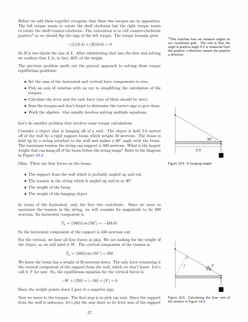
Before we add these together recognize that these two torques are in opposition.The left torque wants to rotate the shelf clockwise but the right torque wantsto rotate the shelf counter-clockwise. The convention is to call counter-clockwisepositive2 so we should flip the sign of the left torque. The torque formula gives

2This matches how we measure angles onour coordinate grid. The rule is that theangle is positive angle if it is measured fromthe positive x-direction toward the positivey-direction.

−(L)(0.4) + (R)(0.6) = 0

So R is two-thirds the size of L. After substituting that into the first and solvingwe confirm that L is, in fact, 60% of the weight.

The previous problem spells out the general approach to solving these torqueequilibrium problems:

• Set the sum of the horizontal and vertical force components to zero.

• Pick an axis of rotation with an eye to simplifying the calculation of thetorques.

• Calculate the lever arm for each force (one of them should be zero).

• Sum the torques and don’t forget to determine the correct sign to give them.

• Work the algebra—this usually involves solving multiple equations.

Let’s do another problem that involves some torque calculations.

Consider a object that is hanging off of a wall. The object is held 2.0 metersoff of the wall by a rigid support beam which weighs 50 newtons. The beam isheld up by a string attached to the wall and makes a 30 angle with the beam.The maximum tension the string can support is 500 newtons. What is the largestweight that can hang off of the beam before the string snaps? Refer to the diagramin Figure 10.4.

30

2.0

Figure 10.4: A hanging weightOkay. There are four forces on the beam:

• The support from the wall which is probably angled up and out

• The tension in the string which is angled up and in at 30

• The weight of the beam

• The weight of the hanging object

In terms of the horizontal, only the first two contribute. Since we want tomaximize the tension in the string, we will consider its magnitude to be 500newtons. Its horizontal component is

Tx = (500)(cos 150) = −433.01

So the horizontal component of the support is 433 newtons out.

For the vertical, we have all four forces in play. We are looking for the weight ofthe object, so we will label it W . The vertical component of the tension is

Ty = (500)(sin 150) = 250

We know the beam has a weight of 50 newtons down. The only force remaining isthe vertical component of the support from the wall, which we don’t know. Let’scall it F for now. So, the equilibrium equation for the vertical forces is

−W + (250) + (−50) + (F ) = 0

Since the weight points down I gave it a negative sign.

T`

Figure 10.5: Calculating the lever arm ofthe tension in Figure 10.4

Now we move to the torques. The first step is to pick our axis. Since the supportfrom the wall is unknown, let’s put the axis there so its lever arm of the support

57

will be zero. The weight of the beam is concentrated at its center3, so it has a3This point is called the center of gravity.It coincides with the center of mass unlessthe force involved varies over the configu-ration of the system. For standard gravity(i.e., weight) the force is constant so thereis no difference.

lever arm of one meter. The hanging object has a lever arm of two meters. Thelast one to determine is the lever arm of the tension. The line of action is alongthe string, so the dotted line in Figure 10.5 represents the lever arm. This line isthe opposite side of a right triangle whose hypotenuse is the length of the beam.The cosine connects the two. Therefore

` = (2)(cos 30) = 1

Force Magnitude Lever Arm Direction Torque

Tension 500 1 + 500

Beam weight 50 1 − −50

Object weight W 2 − −2W

Table 10.1: The torque calculations for Figure 10.4

Table 10.1 summarizes what we have so far. I have left off the support from thewall since we deliberately set its torque to zero. These torques have to add up tozero, so

(500) + (−50) + (−2W ) = 0

Well here is a surprise. We can simply solve for W directly from the torqueequation. The maximum weight the beam can hold is 225 newtons.

A couple of notes from this solution. Notice how we were able to avoid a bunchof math by picking our axis to zero out the support force. In fact, we never evenneeded to look at the horizontal and vertical components of the forces.

The second thing is that the calculation of the lever arm for the support was theworst part of the problem. This is usually the case. It always comes down tofinding a right triangle and using our trig. If you have multiple lever arms tofind, this can be quite annoying. Another approach is to calculate the torquetangentially. In this problem that means we need to determine the verticalcomponent of the tension—which we calculated earlier as 250 newtons. Sincethe distance from the axis for this force was two meters, this also yields a torqueof 500 newton-meters. You can see that this approach gets to the torque muchfaster.

Depending on the information given in your problem you might consider usingone or the other approach. In the end they are equivalent, so it’s up to you.

We are now ready to consider non-equilibrium problems in which the torquesdo not cancel. You may worry that this will be unbearably difficult given thecomplications involved in solving the corresponding torque equilibrium problems.However, we’ve done most of the heavy lifting already, so take heart.

Suppose we have a particle attached by a small rod to a particular point in spacewithout any external forces. If in motion, it will move with uniform circularmotion. This is because the centripetal force from the rod is always perpendicularto the motion, so the speed will not change. We can summarize this by sayingthat the angular acceleration of the particle is zero. This is analogous to Newton’sfirst law of motion.

Now suppose we apply a force to the particle. Any component of the forceperpendicular to its motion will be counter-balanced by the rod, so we only needconsider a force parallel with the motion. This force will accelerate the particleaccording to Newton’s second law, equation (5.1). We also know that torque isrelated to force via τ = Fr and acceleration to angular acceleration via a = rα.So we can rewrite Newton’s second law as

(τ/r) = (m)(rα)

58

or, more suggestively,

τ = Iα (10.1)

where I = mr2 is called the moment of inertia for the particle. Equation (10.1)represents the angular analog of Newton’s second law.

For an extended rigid object, this formula is the same. Essentially, the extendedobject can be considered as a (large) collection of particles, so the moment ofinertia in general is

I =∑

mr2 (10.2)

If mass measures the tendency of an object to maintain its linear motion thenthis moment of inertia measures the tendency of an object to maintain its angularmotion. The moment of inertia depends not only on the total mass but also onthe distribution of that mass throughout the object.

For simple shapes, the formula for the moment of inertia can be written in termsof the total mass. For example, a hollow sphere rotating through its center has amoment of inertia of 2

3MR2. See Table 10.2 for a more complete list.

Ring MR2

Disk 12MR

2

Sphere 25MR

2

Shell 23MR

2

Rod (center) 112ML

2

Rod (edge) 13ML

2

Table 10.2: Moment of inertia for varioussystems. See here for more.

Consider the following example. A disk has a radius of 0.10 meters and a mass of2.0 kilograms. It is attached on-center to a circular post (radius = 0.01 meters)which allows it to rotate horizontally (assume no friction). An ideal string iswound around the post and is attached to a 0.5-kilogram object that is hangingover a pulley. As this object falls, the disk rotates. After three seconds, how fastis the disk rotating? See Figure 10.6

a

Figure 10.6: Rotating disk attached to aweight

The disk begins rotating because of the torque applied from the string. Sincethis is a non-equilibrium problem, we should not assume the tension in the stringequals the weight of the hanging object—it will be less because the mass falls. Infact, Newton’s second law tells us that

T −mg = −ma

where T is the tension in the string and m is the mass of the hanging object.This is just like in the inclined plane example on page 23. So we have a formulabetween the tension and the acceleration:

T = 9.8− (0.5)(a)

Now consider the disk. For this we have Newton’s second law in its angular form(10.1). The moment of inertia for a disk is I = 1

2MR2, so for this problem we

have

I = 12 (2.0)(0.10)2 = 0.020

The torque is from the tension in the string which it is applied to the post, so thelever arm is its radius:

τ = (T )(0.01)

The angular acceleration of the disk can be gotten from equation (10.1):

(T )(0.01) = (0.020)(α) =⇒ α = (0.5)(T )

Using the previous expression for the tension yields

α = 4.8990− (0.25)(a)

Now, which radius do we use in a = rα to solve this equation? The accelerationof the block is equal to the tangential acceleration of the post because these areconnected by the string. So, a = (0.01)(α). Since we are asked about the diskrather than the object, we should use this to solve for the the angular acceleration:

α = 4.8990− (0.02)(0.01)(α)

59

So α = 4.8990. In order to answer the question we should use the angular analogof equation 3.6:

ω2 = (0)2 + (2)(4.8990)(3) =⇒ ω = 5.4216

After three seconds the disk is rotating at 5.4 radians per second, or just under52 rpm.

Shall we do another? Suppose a sphere rolls down an incline of 30 which is 4.0meters long without slipping. How fast is it moving at the bottom of the incline?

For this one we will use energy. Since causing an object to rotate requires work,we expect a formula similar to equation (7.2) for the kinetic energy of rotation:

KErot = 12Iω

2

In this case, all the initial energy is potential. The sphere is at a height of 2.0meters, so its potential energy is

PE = (m)(9.8)(2.0) = (19.6)(m)

At the bottom of the slope this potential energy is converted into kinetic, but thekinetic energy is split between linear motion and rotation:

(19.6)(m) = 12mv

2 + 12Iω

2

We know the sphere does not slip, so we also have v = rω and the moment ofinertia for a sphere is 2

5MR2. Since we are asked for the speed we combine these

to write(19.6)(m) = 1

2mv2 + 1

2 ( 25mr

2)(v/r)2

or,19.6 = 7

10v2

The final speed will be 5.3 meters per second. This speed is independent of themass and radius of the sphere.

In addition to kinetic energy we also have a rotational analog for momentum.The angular momentum of a system is

L = Iω (10.3)

which just like linear momentum is conserved in any collision (assuming noexternal torque). This conservation is why it is easier to ride a bike that ismoving than balancing on one that is stationary. Once the angular momentumof the wheels is built up, they tend to continue rotating along the same axis.

That completes the analogy between linear motion and rotation. Except we haveonly scratched the surface. So far we have only discussed rotation in a plane witha fixed axis. We have yet to talk about free rotation. In general as an objecttumbles it rotates with a wobble. In order to understand this we will need torefine our description of rotation.

Since each rotation involves a magnitude (the angular speed) and a direction(the axis of rotation), we can talk about it like a vector. For fixed rotation in aplane, this vector points out of the plane.4 In addition, we can associate angular

4Whether it point out or in is arbitrary. It isconventional to consider the vector as point-ing at you when you are looking at counter-clockwise rotation. This is consistent withthe xyz axes in the sense that rotation fromthe positive x-direction to the positive y-direction points in the positive z-direction.

acceleration, torque, and angular momentum with vectors.

How then do we explain the wobble? It happens that, for any shape object,there are certain principal axes about which the object will rotate without thiswobble. In this case the angular velocity vectors and the angular momentumvectors are aligned. For rotation off of these axes, the two are not aligned. Thedistribution of the mass throws off the balance of the rotation.

Since the distribution of mass is captured in the moment of inertia, the angularmomentum captures both the rotation and this distribution. And since the

60

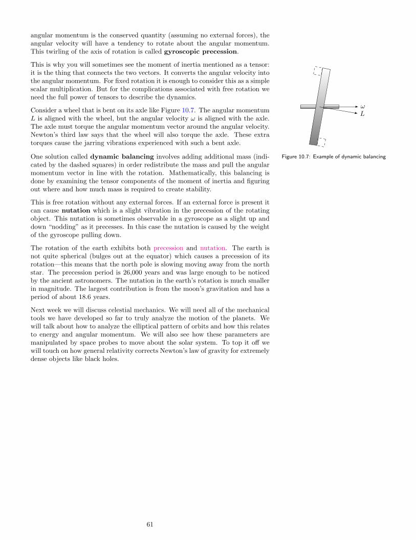
angular momentum is the conserved quantity (assuming no external forces), theangular velocity will have a tendency to rotate about the angular momentum.This twirling of the axis of rotation is called gyroscopic precession.

This is why you will sometimes see the moment of inertia mentioned as a tensor:it is the thing that connects the two vectors. It converts the angular velocity intothe angular momentum. For fixed rotation it is enough to consider this as a simplescalar multiplication. But for the complications associated with free rotation weneed the full power of tensors to describe the dynamics.

Consider a wheel that is bent on its axle like Figure 10.7. The angular momentumL is aligned with the wheel, but the angular velocity ω is aligned with the axle.The axle must torque the angular momentum vector around the angular velocity.Newton’s third law says that the wheel will also torque the axle. These extratorques cause the jarring vibrations experienced with such a bent axle.

ωL

Figure 10.7: Example of dynamic balancingOne solution called dynamic balancing involves adding additional mass (indi-cated by the dashed squares) in order redistribute the mass and pull the angularmomentum vector in line with the rotation. Mathematically, this balancing isdone by examining the tensor components of the moment of inertia and figuringout where and how much mass is required to create stability.

This is free rotation without any external forces. If an external force is present itcan cause nutation which is a slight vibration in the precession of the rotatingobject. This nutation is sometimes observable in a gyroscope as a slight up anddown “nodding” as it precesses. In this case the nutation is caused by the weightof the gyroscope pulling down.

The rotation of the earth exhibits both precession and nutation. The earth isnot quite spherical (bulges out at the equator) which causes a precession of itsrotation—this means that the north pole is slowing moving away from the northstar. The precession period is 26,000 years and was large enough to be noticedby the ancient astronomers. The nutation in the earth’s rotation is much smallerin magnitude. The largest contribution is from the moon’s gravitation and has aperiod of about 18.6 years.

Next week we will discuss celestial mechanics. We will need all of the mechanicaltools we have developed so far to truly analyze the motion of the planets. Wewill talk about how to analyze the elliptical pattern of orbits and how this relatesto energy and angular momentum. We will also see how these parameters aremanipulated by space probes to move about the solar system. To top it off wewill touch on how general relativity corrects Newton’s law of gravity for extremelydense objects like black holes.

61

62

Lecture 11

Celestial MechanicsReview lectures 6, 7, 9, and 10

We’ve already shown how Newton’s law of gravity, equation (6.3) can be used toestablish Kepler’s third law (see page 35). We can now show that the second lawfollows from the conservation of angular momentum.

The moment of inertia for a particle rotating about an axis is simply mr2 where ris the distance from the axis. The angular momentum of this particle is therefore

L = (mr2)(ω) = mrvt (11.1)

where we have used the fact that vt = rω.

If we look at the position of the particle between two points in time we will geta diagram like Figure 11.1. The triangle defined by these positions has a heightequal to vt ∆t and we can say it has a base equal to r. So this area is given by

A = 12rvt ∆t = 1

2 (L/m) ∆t

r1

r2

v ∆t

vt ∆t

Figure 11.1: Kepler’s second law and angu-lar momentum

Since the force of gravity is central, its line of action runs through the centralpoint. This means it has no lever arm and produces no torque. As a consequence,the angular momentum is conserved. Therefore the area swept out by the radiusvector is equal for equal time periods—which is Kepler’s second law.

Kepler’s first law is more difficult to derive. We’ll skip the proof and move on tolearning a few things about calculating with ellipses.

For problems in celestial mechanics, it is easiest to use polar coordinates. In orderto consider problems relevant to Kepler’s first law, we will consider an ellipse withits focus at the origin of a system of polar coordinates. In addition, assume theθ = 0 line is aligned with major axis of the ellipse like in Figure 11.2.

The point of closest approach for the planet is called perihelion. The suffix“helion” refers to the sun. If we are talking about orbiting the earth, the correctterm would be perigee (the general term is periapsis). We will give this the labelr0.

On the opposite side of the ellipse we have the aphelion which is the point offarthest excursion. For the earth we say “apogee” and in general we say “apoasis”.We will label this point r1.

Both of these points lie on the major axis of the ellipse. So these three parametersare related by the following formula:

r0 + r1 = 2a (11.2)

63

Figure 11.2: Key parameters and definitions for an ellipse

Focus

Center

Perihelion Aphelion

r0 r1

a a

r

θ

where a is the semi-major axis (i.e., half of the major axis).

The equation that describes the shape of the ellipse in polar coordinates is

r = r01 + e

1 + e cos θ(11.3)

where e is called the eccentricity of the ellipse. An eccentricity of zero corre-sponds to a perfect circle. Ellipses are characterized by an eccentricity less thanone—the larger the number, the flatter the shape.1 Notice that equation (11.3)

1We can incorporate unbound orbits byallowing the eccentricity to be greater thanone.

does not involve time. This is merely an equation to describe the geometry of thepath.

The more eccentric the ellipse, the farther the focus is from the center. Thisdistance is half of r1 − r0. It happens that the formula for the eccentricity is

e =r1 − r0

r1 + r0(11.4)

which is just this distance normalized by the semi-major axis of the ellipse.

The ellipse is characterized geometrically by the parameters a (the size of theellipse) and e (the shape of the ellipse). Equations (11.2) and (11.4) show how tomove back and forth between these parameters and the observable parameters r0

and r1. These facts are the bare minimum we need in order to understand thebasics of celestial motion.

Now we are ready to discuss some dynamics. The potential energy function forgravity is given by equation (7.4). It is possible to reduce the two-dimensionalmotion of the planet to one dimension by using a rotating reference frame tied tothe planet. Use of this frame will introduce a centrifugal force given by equation(9.6). We can use the conservation of angular momentum to eliminate the angularvelocity from this expression. Since L = mrω2, we have

Fcfg =L2

mr3

This is similar to the formula for gravity (6.3) and there is a corresponding“potential energy” associated with it. If we combine this with the potentialenergy for gravity, we have the following:

U = −GMm

r+

L2

2mr2(11.5)

This is called the effective potential and acts as the potential energy for theradial motion of the planet. (See Figure 11.3). Any orbital energy above the

64

effective potential is kinetic. Remember this is the kinetic energy associatedwith the radial motion not the angular motion. The centrifugal term is themanifestation of the angular motion. In fact, using equation (11.1) one can seethat the centrifugal “potential” can also be written at 1

2mv2t . So this term can

be seen as either potential or kinetic.

r

E

Inverse square law: −GMm/r

Centrifugal force: L2/2mr2

E0E0

r0 r1

Emin

Figure 11.3: The effective potential for gravity

Note that the effective potential depends implicitly on the angular motion of theplanet through the angular momentum L. The faster it rotates, the larger thecentrifugal term, and the farther away will be the point of closest approach. Theminimum point (Emin) on the effective potential corresponds to a purely circularorbit because the radius does not change—it has no kinetic energy of motion inthe radial direction.

The effective potential gives us enough information to connect the motion of theplanet to its dynamics. Specifically we can determine the relationship betweenthe orbital energy and angular momentum (the dynamical parameters) to its per-ihelion and aphelion because they are the turning points on the energy diagram.We have already seen that these points are directly related to the eccentricity andsemi-major axis of the ellipse (the orbital parameters).

The turning points are determined by setting the effective potential equal to thetotal orbital energy of the planet and solving for r. But the effective potential(11.5) makes it look like the orbit of the planet depends on its mass, which it doesnot. The acceleration due to gravity is independent of the mass of the object,so should the orbit of the planets. In order to emphasize this, let’s introducethe “reduced” quantities E′ = E/m and L′ = L/m. In fact, I’ll even dropthe primes and simply use the reduced versions because we rarely need to knowthe original ones. Multiplying both sides by 2mr2 and rearranging yields thequadratic equation we now need to solve:

2Er2 + 2GMr − L2 = 0

Determining both the eccentricity and the semi-major axis involve the sum anddifference of the solutions to this equation.2 For the sum we have:

2For a general quadratic equation, ax2 +bx+c = 0, the sum of the solutions is −b/aand their difference is

√(b/2a)2 − (c/a).

r1 + r0 = −GM/E

and the difference is:

r1 − r0 =

√(GM

2E

)2

+L2

2E

The semi-major axis of the ellipse is half the sum of the perihelion and aphelion(11.2), so

a = −GM/2E (11.6)

65

and the eccentricity is the ratio of the difference to the sum (11.4), so

e =

√1

4+

EL2

2(GM)2(11.7)

These results are enough for us to start working some problems.

Consider a rocket satellite orbiting around the earth in a circular orbit with radiusof 4.5× 107 m. A sudden blast of the rocket motor increases the speed by 15% inthe direction of motion. See Figure 11.4. Find (a) the maximum distance of therocket, and (b) the eccentricity of the new orbit.

r0 = 4.5× 107

r1

∆v = 0.15 v0

Figure 11.4: Rocket blast problem

Ever thought you’d be a rocket scientist? The quantity GM occurs frequently, solet’s make a note of the product:

GM = (6.673× 10−11)(5.9742× 1024)

= 3.9866× 1014

In this case M is the mass of the earth. Back in Lecture 6, we discussed Kepler’sthird law. In the process we derived the formula GM = rv2 for circular orbits(see page 35). We can use this to determine the velocity of the satellite beforethe blast.

(3.9866× 1014) = (4.5× 107)(v0)2

=⇒ v0 = 2976.4

The blast occurs in the direction of motion, so all of the ∆v is tangential and thevelocity after the blast must be

v = (1.15)(v0) = 3422.9

Since the new orbit is not circular, the speed of the satellite will not always havethis value. However, this point does now act as perigee for the new orbit (seeFigure 11.4). Since we know the distance and velocity at this point, we cancalculate the reduced energy and angular momentum.

There are a couple of ways to get at the total (reduced) energy, but perhaps thesimplest is to simply take the sum of the (reduced) kinetic and potential energies:

E = 12v

2 −GM/r

= 12 (3422.9)2 − 3.9866× 1014

4.5× 107

= −3.0010× 106

The energy is negative because the satellite is still in a bound orbit. The angularmomentum is also straight-forward to calculate because at perigee (and apogee)all the velocity is tangential.

L = rvt

= (4.5× 107)(3422.9)

= 1.5403× 1011

Having calculated the dynamical parameters for the orbit, it remains to determinethe orbital parameters. Using equation (11.6), we get

a = − (3.9866× 1014)

(2)(−3.0010× 106)

= 6.6421× 107

Now equation (11.2) yields the apogee:

r1 = 8.7842× 107

66

And equation (11.4) yields the eccentricity:

e = 0.32251

So, the final answer is 8.8 × 107 meters for farthest excursion and the orbit hasan eccentricity of 0.32.

When we talk about the motion of the planets, Kepler’s laws are a good firstapproximation—they describe the motion of each planet around the sun. Whatthey don’t take into account is the interaction between the planets. For example,the pull of Jupiter will cause each other planet to deviate slightly from a pureKeplerian ellipse.

In general, any slight deviation from the central inverse square law will manifestitself as a slight orbital precession. That is, the axis of the ellipse will itselfslowly rotate causing the orbit to not quite close, like a spirograph. In Figure11.5 this angle is denoted by measuring the movement of aphelion, although it istypically easier to measure the precession of perihelion.

∆φ

Figure 11.5: Measuring orbital precessionWith the improvement in observations and calculations over time, the orbits ofall the planets were explained—including the discovery of Neptune and Pluto. Bythe middle of the 19th century, the slight irregularities and precession in Kepler’sorbits were fully explained by Newton’s law of gravity, except one. After takinginto account all effects, there still remained a 43 arc-second per century precessionin Mercury’s orbit unaccounted for (this is a little over 7% of the total precessionobserved). This discrepancy was unresolved until 1916 and Einstein’s generalrelativity.

r

E

Newtonian gravity

E0E0

Figure 11.6: The effective potential in general relativity

Although general relativity requires a significant amount of math to fully appreci-ate, we can learn a bit about its consequences. For us, the easiest impact to see ison the effective potential. General relativity adds a new term to the calculation.The complete (reduced) effective potential is3

3This equation is exact—no slow speed orsmall mass approximation is necessary.

U = −GMr

+L2

2r2− GM

c2L2

r3(11.8)

This revised effective potential is plotted in Figure 11.6. The third term causes aprecession which Einstein calculated as

∆φ =6π

a(1− e2)

GM

c2(11.9)

where a and e are the semi-major axis and eccentricity of the orbit, respectively.This formula explains the anomalous precession of Mercury and was one of thethree initial successes of Einstein’s new theory of gravity.4 The quantity GM/c2

4The other two were gravitational redshiftand the deflection of starlight.

67

is characteristic of the effects of general relativity.

You can see that the new term predicts a slightly stronger law of gravity thanNewton’s. Ultimately this comes from the fact that E = mc2, so the gravitationalfield itself acts as a source of gravity. Both the equilibrium point and perihelionare pulled a little closer. But more dramatically, if the incoming object hassufficient energy the gravitation well will capture it regardless of the centrifugalforce.

This point of no return is called the Schwarzschild radius, rs = 2GM/c2. Ifan object is crushed below its own Schwarzschild radius, it will not be able toprevent its own collapse—a black hole will result. That is why this distance istraditionally called the radius of a black hole even though it really does not haveany extension. Notice that black holes do not require a lot of mass—what theyrequire is an extremely dense mass.

Of course, black holes are only one of the dramatic predictions of general relativity.We don’t have time to cover them all: curvature of space-time, gravitationalwaves, expansion of the universe, the existence of “dark energy”.5 General

5See Lecture 13 and 26 for more info. relativity has withstood the test of time and stands today as one of the twopillars of fundamental physics.6 It also represents the end the road for this term

6The standard model is the other pillarwhich we will cover in Lecture 30.

regarding the motion of simple objects.

68

Lecture 12

Harmonic MotionRead sections 10.1–10.6

In Lecture 7 we discussed the fact that nearly all physical systems sit in a stateof stable equilibrium (see page 41). A state is in stable equilibrium if the internalforces of the system tend to push it back into that state. This must be truealong all the degrees of freedom for the system. For example, a rigid object isin equilibrium only if both the forces and the torques in the system are balanced(see Lecture 10).

If the system is somehow displaced from this point of equilibrium, it will bepushed back. As the system returns to this equilibrium state, its inertia will tendto carry it through and past equilibrium. So the system touches its equilibriumonly to move away in the opposite direction. Eventually the forces in the systembecome large enough to overcome the inertia of the motion, bring it to a stop,and push it back toward equilibrium. Eventually the system will be back to thedisplaced state in which it started. And the cycle repeats over and over. Thisback-and-forth motion is called vibration and a system can vibrate along any ofits degrees of freedom, whether that is a spring, a string, the surface of a drum,a metal beam, a column of air, or the electromagnetic field.

The maximum extent of the displacement is called the amplitude of the motionand the time it takes for one complete cycle is called the period of the motion. Itis no coincidence that this is the same term we used in Lecture 6. The reciprocal ofthe period is called frequency and its unit is the hertz—so when the vibrationof a system is said to have a frequency of 10 hertz, we mean that its motionrepeats 10 times each second.

The simplest example of a vibrating system is a spring with one end attachedto a fixed point and the other end attached to a certain mass. We will assumethe spring is oriented horizontally to ignore gravity and we will assume the massslides without friction (see Figure 12.1).

Figure 12.1: The simplest vibrating system:an ideal spring

This system is in equilibrium when the spring is not stretched. We define theposition of the mass to be zero at this point. Any displacement to the right willbe positive, and any displacement to the left will be negative. In either case, thespring will exert a force that will tend to restore the mass to equilibrium. In otherwords, the mass will experience a force that is in opposition to its displacement.The spring is considered an ideal spring if the magnitude of this force is exactlyproportional to the displacement. In symbols, the restorative force of an idealspring is

F = −kx (12.1)

where k is called the spring constant and is measured in newtons-per-meter andthis equation is frequently called Hooke’s Law. The motion of a mass subject

69

to this force law is called simple harmonic motion.

When our simple mass-and-spring system is vibrating, the restorative force willchange in time as it responds to the motion of the mass. This means that theconstant acceleration equations from Lecture 3 will not be applicable to thissystem. We need a different way to analyze this kind of vibrating motion. Thisis similar to the situation we faced in Lecture 6 with uniform circular motion,except we now know the force but not the mathematics of the motion.

All is not lost. By a fortunate fluke, we can leverage our learnings from Lecture6 to help us now. Consider the projection of uniform circular motion onto thex-axis. Figure 12.2 shows the essential correspondences.

r = A ; θ = ωt

x(t) = A cos(ωt)

xmax = A

v =2πr

T= Aω

v(t) = Aω sin(ωt)

vmax = Aω

a =v2

r= Aω2

a(t) = −Aω2 cos(ωt)

amax = Aω2

Figure 12.2: Uniform circular motion versus simple harmonic motion

The position of the particle in uniform circular motion is specified by its radiusand its angle. Since the motion is uniform, the angle increases at a constant rate,so we have θ = ωt, where ω is the angular speed of the particle. The projectionof this position onto the x-axis involves a right triangle. The diagrams on thebottom of Figure 12.2 show this projection: the position of this particle is givenby

x(t) = A cosωt (12.2)

where we have also relabeled the radius as A since this is also the amplitude ofthe projected motion.

In Lecture 6 we found that the acceleration in uniform circular motion is directedin toward the center. Since this is directly opposed to the position vector, the sameis true in the projection. That is, the acceleration is opposed and proportionalto the position. This is precisely the kind of connection we expect with an idealspring.

In fact, we can say more. We know that the speed of the uniform circular motionis related to the radius and period of the motion via v = 2πr/T . By definition, theangular speed is the 2π radians divided by the time period T , so we can rewritethis as v = Aω. (This should also remind you of the formula for tangentialvelocity (9.3) in Lecture 9.) Since this velocity vector is pointing perpendicularto the position vector, the projection of the velocity is given by

v(t) = Aω sinωt (12.3)

70

The formula for the acceleration in uniform circular motion is from equation (6.1).Using our work so far, we can rewrite this as a = Aω2. Since the projection isopposed to the displacement, the formula for the acceleration of simple harmonicmotion is given by

a(t) = −Aω2 cosωt (12.4)

We can get to this same spot without the analogy to circular motion using abit of calculus. Those of you familiar with those techniques will recognize theconnections between the sinusoidal functions here. In either case, equations(12.2)–(12.4) describe the kinematics of simple harmonic motion.

In the preceding, we have assumed the particle begins at its point of maximumextension. We can remove this restriction by adding an extra term to equation(12.2):

x(t) = A cos(ωt+ φ) (12.5)

The quantity φ is called the phase shift and will become important when wediscuss wave interference in Lecture 19. Any system which obeys equation (12.5)is called a simple harmonic oscillator.

It remains to connect these considerations with the parameters of our ideal springsystem. We can put together Hooke’s law (12.1) with Newton’s second law (5.1)to get

−kx = ma

After plugging in the results from equations (12.2) and (12.4) and simplifying weget

k = mω2 (12.6)

This little equation is an important summary of the dynamics of the ideal spring.In general, any vibrating system will have a similar equation connecting theparameters of the system to the frequency of its motion. The value of ω iscalled angular frequency to distinguish it from the vibration frequency definedearlier. Because there are 2π radians in each cycle, the two quantities are simplyconnected by the equation ω = 2πf . So, we can write the vibration frequency ofthe simple harmonic motion in terms of the spring constant and the mass:

f =1

2π

√k

m(12.7)

This is called the natural frequency of the ideal spring. For any system instable equilibrium, each degree of freedom will have its own natural frequency.

The amplitude in equation (12.5) is related to the energy in the system. Hooke’slaw (12.1) is conservative and the potential energy associated with it is1

1This can be seen from the definition ofwork (7.1)

∆W = F∆x

In this case we have to be careful becausethe force is not constant. But the workdoes increase at a constant rate, so weuse the trick from Lecture 3 where theaverage value is equal to the average ofthe ends. In this case, the work done atthe beginning is zero because there is nonet force at equilibrium. As we pull onthe spring, the work required increases. Atfull extension, the work required is W =(−kx)(x). Taking the average introduces afactor of one-half.

PEspr = 12kx

2 (12.8)

In general, the total energy of the ideal spring system is sum of the kinetic energyof the mass and the potential energy in the spring. But when the system is atmaximum extension the velocity of the mass is zero (for a moment). Since x = Aat this point, we can write

Etot = 12kA

2 (12.9)

The fact that the energy of vibration is proportional to the square of the amplitudeof the vibration explains why laser light is so much more powerful than regularlight (see Lecture 27).

Hooke’s law (12.1) is an idealization for a real spring, and even more so forcomplex physical systems. However, the forces maintaining any state of stableequilibrium are approximately linear for small displacements. One easy way tosee this is by investigating the energy diagram. For a system to be in stableequilibrium, the potential energy curve must create a trough or potential well.The point of equilibrium is at the bottom of this well. If one were to fix the vertex

71

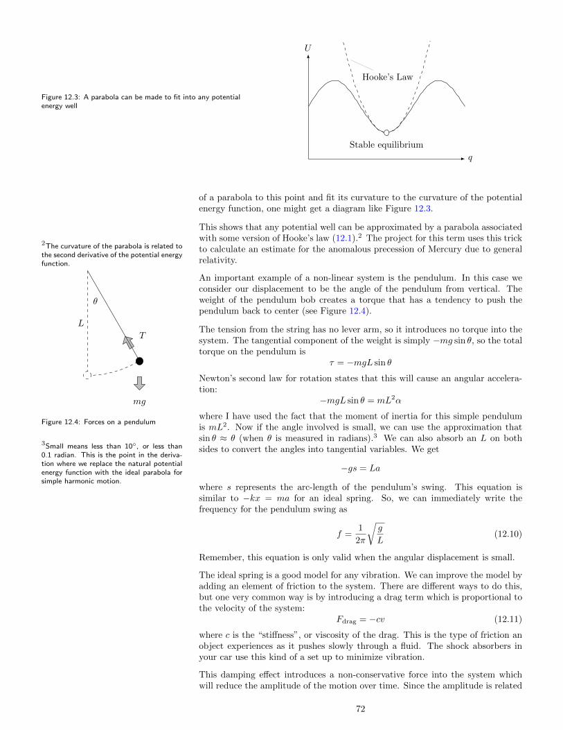
Figure 12.3: A parabola can be made to fit into any potentialenergy well

q

U

Stable equilibrium

Hooke’s Law

of a parabola to this point and fit its curvature to the curvature of the potentialenergy function, one might get a diagram like Figure 12.3.

This shows that any potential well can be approximated by a parabola associatedwith some version of Hooke’s law (12.1).2 The project for this term uses this trick

2The curvature of the parabola is related tothe second derivative of the potential energyfunction.

to calculate an estimate for the anomalous precession of Mercury due to generalrelativity.

An important example of a non-linear system is the pendulum. In this case weconsider our displacement to be the angle of the pendulum from vertical. Theweight of the pendulum bob creates a torque that has a tendency to push thependulum back to center (see Figure 12.4).

L

θ

T

mg

Figure 12.4: Forces on a pendulum

The tension from the string has no lever arm, so it introduces no torque into thesystem. The tangential component of the weight is simply −mg sin θ, so the totaltorque on the pendulum is

τ = −mgL sin θ

Newton’s second law for rotation states that this will cause an angular accelera-tion:

−mgL sin θ = mL2α

where I have used the fact that the moment of inertia for this simple pendulumis mL2. Now if the angle involved is small, we can use the approximation thatsin θ ≈ θ (when θ is measured in radians).3 We can also absorb an L on both

3Small means less than 10, or less than0.1 radian. This is the point in the deriva-tion where we replace the natural potentialenergy function with the ideal parabola forsimple harmonic motion.

sides to convert the angles into tangential variables. We get

−gs = La

where s represents the arc-length of the pendulum’s swing. This equation issimilar to −kx = ma for an ideal spring. So, we can immediately write thefrequency for the pendulum swing as

f =1

2π

√g

L(12.10)

Remember, this equation is only valid when the angular displacement is small.

The ideal spring is a good model for any vibration. We can improve the model byadding an element of friction to the system. There are different ways to do this,but one very common way is by introducing a drag term which is proportional tothe velocity of the system:

Fdrag = −cv (12.11)

where c is the “stiffness”, or viscosity of the drag. This is the type of friction anobject experiences as it pushes slowly through a fluid. The shock absorbers inyour car use this kind of a set up to minimize vibration.

This damping effect introduces a non-conservative force into the system whichwill reduce the amplitude of the motion over time. Since the amplitude is related

72

to the energy of this system, this reflects the fact that energy is being lost throughfriction. The equation for the amplitude is

A(t) = A0 exp(−γt)

where γ = c/2m. The displacement of the damped oscillator over time is graphedin Figure 12.5.

x

t

Figure 12.5: The motion of a dampedharmonic oscillator

When γ = ω, the system is said to be critically damped. This is the circum-stance which brings the system back to equilibrium the fastest. If the system isunder-damped (γ < ω), then it will oscillate a bit before being brought to rest,as described above. If the system is over-damped (γ > ω), then the viscosity willbe so thick it will actually drag against the system being brought to rest.

Finally, we have one last topic to consider: forced vibrations. If a damped systemis driven by an external vibration, the motion of the system will eventually matchthe frequency of the driver. Initially it will move through a temporary (∆t > 1/γ)transient state until it reaches a steady state of sinusoidal motion. This steadystate will have an amplitude which will depend upon both the frequency of theexternal driver and the natural frequency of the system.

What happens is that the external vibration does work on the system when theforce is aligned with the displacement of the system. When the frequency of theexternal vibration is matched with the natural frequency of the system, the workdone in each cycle accumulates. It does not take long for system to absorb a lotof energy from the external source even if the magnitude of the source is small.Eventually the system is moving fast enough that the damping force (proportionalto this speed) increases to drain the energy that is being absorbed. This steadystate is called resonance.

The typical power absorption for a driven harmonic oscillator is plotted in Figure12.6. The peak power absorption occurs at the natural frequency of the system.The width of the peak is related to the “stiffness” of the damping: at one-half ofthe maximum power absorption it is equal to 2γ.

P

fext

f = ω/2π

12Pmax

2γ Figure 12.6: Power absorption in a driven harmonic oscillator

Resonance can be used to explain the scattering of light (why the sky is blue),how microwaves work, and is important in certain electrical circuits. The qualityfactor of an electrical circuit is defined as the ratio of the resonant frequency andthe half-maximum width of the power absorption curve. A sharp peak will make agood radio receiver as it will only react to a particular range of radio frequencies.A quality factor between 10 and 100 is common. For our ideal spring, this qualityfactor would be

Q =ω

2γ=

√km

c2

which shows how this one metric incorporates all the essential parameters of thesystem.4

4The quality factor for a resonating circuitis

√L/CR2—see Lecture 25.

73

Next lecture we will extend this notion of things that stretch to cover the topicof the elasticity of solids. We will find that forces create stress in an elastic solidand that this stress can be decomposed into three essential components. Stresscauses strain, and Hooke’s law will reappear in the relationship between them.We will take a quick overview of the various ways real objects deform and reactto various stresses.

The idea of stress also offers us a segue to discuss general relativity. We will seethat the essential effect of gravity is to create stress in the space-time continuum:which is witnessed by the presence of the ocean tides. We will finish by discussingwhether it is possible to avoid being crushed while falling into a black hole.

74

Lecture 13

ElasticityRead sections 10.7–10.8

As discussed in Lecture 1, physics is often described as the study of matter andenergy. So far, we have focused on the dynamics of motion. Now we turn to astudy of the properties of matter—this will occupy us for the next few lectures.The most basic classification of material things is by their phase: whether they aresolid, liquid, or gaseous. At the microscopic level, these phases are distinguishedby the strength of the inter-molecular interaction. The solid phase is such that theconfiguration of the molecules are essentially locked together. They may vibratein place, but there is no bulk motion relative to one another.

In the fluid phases, the molecules can flow around one another and move freely.Both liquids and gases are considered fluids because of their ability to flow. Thetwo are distinguished by the fact that the molecules in liquids stay relativelyclose together (they constantly “touch”), but in gases they fly about nearly freeof interaction.

In this lecture we will discuss solids and their elastic properties. Frequently asolid is depicted as a bunch of molecules connected to one another by springs (seeFigure 13.1). The springs are meant to represent the inter-atomic forces betweenthe molecules. As we discovered in the previous lecture, the forces in any systemnear stable equilibrium can be approximated by ideal springs, so this picture isnot as unrealistic as it may first appear.

Figure 13.1: A solid as a collection ofmolecules connected by springs

This conceptual model also shows the main property of a solid: its elasticity.When any force is applied to a solid, it will respond through deformation andwill resist the force applied. The details of this deformation can be extremelycomplicated—as can be seen just be considering the number of degrees of freedomavailable to all the molecules.

The simplest approach is to consider a solid rod. This is somewhat like a one-dimensional system. Assume the rod is fixed at one end and a force is applied tothe other. In general, the force will have two components: along the length of thebar and across the length of the bar. The first is called normal stress1 and the

1“Normal” because the force is perpendic-ular to the cross-section of the bar.

second shear stress. The reason we use the word stress rather than force hereis that we expect all the forces to be in balance—we are interested not in the netforce which produces motion, but the stable combination of forces which producesdeformation. Stress is what’s left after the net force has been calculated.

Normal stress will either stretch (also known as tension) or compress the solid (seeFigure 13.2).2 The resulting deformation is called the strain in the object and is

2In three dimensions we can distinguishbetween tension and compression by thefact that tension will cause expansion in onedimension and contraction in the other two.Compressive forces will cause expansion intwo dimensions and contraction in one.

defined as the amount of deformation divided by the original length of the bar.The strain is a unit-less number: the percent change in the original length. If theforce is distributed over a large area, the resulting strain will be less. So we are

75

really talking about the pressure from the normal force causing the deformation.When the displacement involved is small, the controlling equation is

F

A= Y

(∆L

L0

)(13.1)

Notice how this is similar in form to Hooke’s law. The quantity Y is calledYoung’s modulus and is on the order of 1011 for metals in SI units (indicatingenormous forces are required to create a significant deformation).

L0A ∆L F

Figure 13.2: A solid rod under normal stress Shear stress is similar, except now we are interested in quantifying the deflectionof the bar (see Figure 13.3). The formula for shear stress is nearly the same:

F

A= S

(∆x

L0

)(13.2)

except now the strain is quantified as the ratio of the deflection to the bar’s length.The proportionality constant S is called the shear modulus.

L0A

∆x

F

Figure 13.3: A solid rod under shear stress We have not exhausted all the ways a solid can be put under stress. You maynotice that in Figure 13.2 there is a slight expansion along the cross-sectional area.The effect is exaggerated in the diagram, but the point is that normal stress willnot change the volume of the object. When one part is squeezed, another willbulge. However, it is possible for forces to completely surround the object like inFigure 13.4. We will call this pressure stress.

Figure 13.4: An object under compressivepressure

In a way you can consider this a special case of normal stress, but we only take theaverage pressure in all directions. In other words, we break the normal stress intotwo components: (1) the average value from all directions (the pressure stress)which changes the volume of the object and (2) the remainder (the normal stressproper) which merely distorts the shape of the object.

The formula for pressure stress is

∆P = −B(

∆V

V0

)(13.3)

where B is called the bulk modulus of the material. The negative sign is herebecause an increase in pressure will cause a decrease in volume.

In the formulas (13.1), (13.2), and (13.3), the forces involved must be small. Infact, they are all similar in form to Hooke’s law (12.1) and are sometimes referredto as such. When the forces become larger, these equations cease to work andtend to over-predict the stress required for a particular level of strain. In otherwords, the object tends to break apart. There are three typical limits of strainfor a given object:

• Proportionality limit

• Elastic limit

• Deformation limit

These are highlighted in Figure 13.5. Up to the proportionality limit, Hooke’s lawis valid and each increment of stress causes a consistent increment of strain. Pastthe proportionality limit and up to the elastic limit, the object is plastic, meaningthat when the stress is removed the object still will conform to its original shape. Ifthe stress exceeds the elastic limit, the deformation is permanent and if the stressgoes beyond the deformation limit, the object will break. Clearly understandingthese limits is important in the design and construction of all kinds of objects.

Now, in general, an object will be under the influence of a variety of forces inmultiple directions at a variety of points. One way to deal with this complexity is

76

Stress (F/A)

Strain (∆L/L0)

Hoo

ke’s

Law

Proportionality limit

Elastic limit

Deformation limit

Hooke’s law is valid

Hooke’s law is not valid

Object is broken

Deformation is permanent

Figure 13.5: Typical stress-strain relationship for a solid object

to break the object into a (large) number of pieces. The simplest way to do thisis by splitting it into little cubes. Each cube interacts with the others throughthe forces along their sides. We deliberately make the cubes so small that we areable to assume the forces are constant along each face. Also, since the cubes aresmall we can apply Hooke’s law to each: in other words, the strain in each cubewill be directly proportional to the forces on the sides. Over the volume of theobject, the strain within the cubes accumulate and gives us the total deformationand deflection in the shape of the object. This approach is called continuummechanics.

Consider the forces on one of these elemental cubes. Since we are only interestedin the stress and not the bulk motion of the cube, we assume the forces are inequilibrium. This means that the forces on opposite sides of the cube are equal andopposite, so we only need consider one side of each pairs. For extreme simplicity,we will consider the two-dimensional “cube” shown in Figure 13.6. The Greekletter σ is traditionally used to denote stress. In our case ~σ(x) represents theforce of stress along the face with the x-direction as its normal. I’ve written itthis way to emphasize the fact that stress σ is a tensor: it maps each directionvector into the force of stress along that direction.3

3Just because it is a function betweenvectors is not enough for it to be a tensor. Itmust also be linear. One could show this byrotating the cube an comparing the resultswith the original orientation.

x~σ(x)

y

~σ(y)

Figure 13.6: Forces of stress on a cubical element

We can go a bit further by breaking these stress vectors into their components.

77

This is shown in Figure 13.7. Each component has a double subscript. The firstletter denotes which cube face we are referring to and the second letter denotesthe direction of the component. For example, σxy represents the y-component ofthe stress force ~σ(x). There are several advantages with this index notation.One of them is that we can easily write that the stress tensor is symmetric, i.e.,σxy = σyx. This is because these are both the tangential components of theirforces and produce torque. But the cube is in equilibrium, so these torques mustcancel. This will only happen if these components are equal.

Figure 13.7: The components of the stress on a cubicalelement

σxy

σxx

σyx

σyy

We can take this even further by busting these components into pieces thatemphasize their normal, shear, and pressure stress dynamics. We have alreadyseen that the shear components are equal by definition, so that is done. Thepressure piece is simply the average of the two normal components. These pressurepieces are also equal by definition. The remaining normal components are alsoequal (though opposite) because they are their difference from the average. Thismeans that we are able to characterize the stress created by arbitrary forces usingjust three numbers related to the three components of stress we introduced atthe beginning of this lecture. Figure 13.8 shows these “canonical” componentsfor the example in Figure 13.6.

Shear

Pressure

Normal

Figure 13.8: The three canonical compo-nents of stress for Figure 13.7

We can even talk about stress on an astronomic scale. The ocean tides resultfrom the stress induced by the gravitational pull of the moon (and the sun). Thegravitational force creates a normal stress on the oceans which tend to expandthe water along the line between the centers of the earth and moon and compressthe water perpendicular to this line.

The expansion can be understood because the inverse square law means that theforce of gravity on the near side to the moon will be slightly larger than at thecenter, which will be slightly larger than on the opposite side. If we label thedistance between the earth and moon d and the radius of the earth as r, we have

Fnear =GMm

(r − d)2

for the force of gravity on the near side. The force on the far side is similar withr + d in the denominator instead.

We can rewrite this equation as

Fnear =

(GMm

d2

)(1− r/d)−2

The reason to do this is that we can use the binomial theorem (1.3) on the secondfactor because r/d is so very small. We have

(1− r/d)−2 ≈ 1 + 2r/d

78

The stress on the earth’s oceans is given by the difference between this force andthat at the center of the earth. For both the near and far sides this is the samein magnitude. We have:

σxx =

(GMm

d2

)2r

d

where the x-direction is aligned along the earth-moon line.

We expect compression on in the y-direction, but the reasoning is different. Inthis case, we are looking for the component of the forces on the sides of the earthdirected toward the center of the earth. The triangle involved in these componentsis similar to the triangle formed by the geometry of the earth-moon system (referto Figure 13.9). This means we can write

F

Fgrav=

r

dside

because in similar triangles the ratio of similar sides are equal.

d

rdside

Figure 13.9: Tides on the earth caused by the gravitationalforce of the moon

The force of gravity Fgrav on the side of the earth is proportional to the inversesquare of the distance dside, or

Fgrav =GMm

d2 + r2

However, by using the binomial theorem earlier, we have implicitly agreed tocompletely ignore r2 relative to d2 since r d.4 By similar logic we can now

4For example, if x = 10−6 is barely in ourmeasurement range then x2 = 10−12 iscertainly not.

write dside = d.

This means that the normal stress across the earth-moon line is

σyy = −(GMm

d2

)r

d

where I have introduced the negative sign since the stress is compressive alongthis component.

The gravitational field introduces no shear stress, so this completely determinesthe tidal stress from the moon.

In classical mechanics we characterize the influence of gravity by Newton’s inversesquare law (6.3). But in Einstein’s general theory of relativity we use these tidalstresses to define the influence of gravity. There are two reasons for this. The firstis that we need a field theory—one that does not involve action-at-a-distance likeNewton’s law. The gravitational effect must propagate through the field at thespeed of light rather than being instantaneous. The second reason is that thereis always an inertial frame in which the force of gravity can be eliminated—thisis the equivalence principle (see page 26). But even in a free-fall frame the tidaleffects of gravity are present. In a way the tidal effects are more “real” than theforce of gravity itself.

So in general relativity, gravity propagates through space as waves of stress in thefabric of space-time. In fact, gravity waves (if detected) will be measured throughtheir extremely faint normal stresses in objects. Only waves from dramaticastronomic events like a supernova will be detectable directly, but there is alreadyindirect evidence of the existence of gravity waves.

79

As one falls into the gravitational well of an object, the free-fall frame experiencestidal forces similar to those from the moon. If the object is a black hole (crushedbeyond is Schwarzschild radius—see Lecture 11), these tidal effects increase with-out limit. As one is pulled inexorably toward the central pit of destruction, thetidal forces will pull one into a long string of spaghetti.

This situation is unavoidable if the black hole is not rotating. If it does rotate(which almost all will since angular momentum is conserved), the event horizonthat surrounds the black hole at its Schwarzschild radius splits in two. And itbecomes possible to pass into the event horizon without being doomed to beingcrushed in the central singularity (the so-called ergosphere). In fact, there iseven reason to believe we can extract energy for the rotation of the black holeby exploiting this ergosphere—this is called a Penrose process. There is evenspeculation that this ergosphere may offer an ability to travel through a black holeto another region of space-time—the worm hole made famous in many sciencefiction stories nowadays. But that discussion lies far afield from this lecture.

Next week we will move on from solids to discuss the dynamics of fluids. Asmentioned earlier, these thoughts will apply to both liquids and gases. Initiallywe will discuss hydrostatics: the properties of fluids at rest. The main resultwill be a determination of the buoyant force in any fluid. After that we move tohydrodynamics, or fluids in motion. We will introduce some new concepts to speakquantitatively about fluid flow and characterize the different ways fluids move.Bernoulli’s equation will be introduced as the main equation for hydrodynamics.We will touch on viscosity which will introduce some realism into our discussion.Finally we will touch on the topic of deterministic chaos which was first discoveredin the study the weather by fluid modeling of the atmosphere.

80

Lecture 14

FluidsRead sections 11.1–11.11

Of the three phases of matter, liquids and solids are distinguished by their abilityto flow. Liquids flow downward under their own weight to take the shape oftheir container while gases flow by expanding to completely fill their container.The ability to transport mass from one point to another is the main thing thatseparates fluids from solids.

This distinction also shows up in how fluids react to the three types of stressintroduced in the last lecture. Fluids don’t break. In fact, fluids can’t reallysupport any normal or shear stress. Although a solid will deform and resist thestress, a fluid will simply react by moving out of the way. An ideal fluid willflow instantly, but any real fluid will have a bit of reaction time related to itsviscosity. This means that pressure is the only kind of stress that a fluid at restwill support.

In fact, a fluid at rest won’t even support a pressure differential. The fluid willmove from high to low pressure. If the pressure increases anywhere in the fluid,this increase will distribute evenly throughout the fluid. This is called Pascal’sprinciple and is what makes most hydraulics work. The hydraulic press is asimple example of this where a force on one end can be used to support a muchlarger force on the other (see Figure 14.1). Since the pressure must be equal andpressure is force divided by area, a larger area will deliver a larger force. Thehydraulic press is a machine with an ideal mechanical advantage equal to theratio of the area on either side of the press.

F1

F2 = 4F1

A1A2 = 4A1

MA =A2

A1

Figure 14.1: The mechanical advantage of the hydraulic press

The statement I made earlier when I said that a fluid will not support a pressuredifferential was not quite true. In the presence of gravity (or any long-range forcefor that matter), the fluid below must support the fluid above.1 In fact, the

1Obviously this requires a container of somesort. Fluid doesn’t just pile up like sand.

pressure differential required is pretty easy to calculate. Imagine a rectangularbox of height h with a horizontal cross-section of area A (see Figure 14.2).

81

We will assume the mass density2 ρ of the fluid is constant, so the total mass of2Remember that mass density is definedas the mass divided by the volume of thesubstance. Later we will see the densitydefined for other quantities like the numberof particles or charge.

this imaginary box of fluid is

m = ρV = ρAh

The pressure on the bottom of the box must exceed the pressure at the top becauseit is holding up the weight of the fluid in the box. The total force from the fluidon the bottom will be F2 = P2A. This force must balance both the pressure atthe top of the box and also the weight of the box. Thus,

P2A = P1A+ ρAhg

When we cancel the area and write in terms of a pressure differential we get:

∆P = ρgh (14.1)

which I like to call the hydrostatic equation.

h

F1 = P1A

F2 = P2A

W

Figure 14.2: Deriving the hydrostatic equa-tion

This reasoning provides us with a method for calculating the force of buoyancyin a fluid. This buoyant force is precisely this pressure differential multipliedby the cross sectional area. In other words

B = ρgV (14.2)

where B is the force of buoyancy, ρ is the density of the fluid, and V is the totalvolume displaced. This equation is sometimes called Archimedes’ principle. Ifthe density of the submerged object is greater than that of the fluid, its weightwill be larger than the buoyant force. The net force will be down and the objectwill sink. If the density of the submerged object is less than the fluid, the objectwill rise until it breaks the surface of the fluid (presuming there is one). After thatpoint, the displaced volume will get smaller until equilibrium is achieved betweenρgV and the weight—the object floats.

Consider a swimming pool. What is the water pressure one meter below thesurface? Well, according to equation (14.1), the answer is 9800 pascals (onepascal is equal to one newton per meter squared), or 9.8 kPa. But this is thepressure differential—what is the pressure at the top of the pool? Hint: It’s notzero.

Yes, the pool is also supporting the weight of all the air above it. The atmospherealso acts like a fluid and this is the source of atmospheric pressure. We are alllike fish swimming is a sea of nitrogen and oxygen gas. The typical value foratmospheric pressure near sea level is 101.3 kPa. So this is the pressure at thetop of the swimming pool. The bottom of the swimming pool will have a absolutepressure of 111.1 kPa.

The pervasiveness of the air makes it easy to ignore. In fact, many tools de-signed to measure pressure (like a tire gauge) are calibrated to register zero atatmospheric pressure. These tools are said to measure gauge pressure whichis simply the true absolute pressure minus one atmosphere’s worth of pressure.Usually we work with pressure differentials so this issue washes out. On the otherhand, occasionally we do need to know the absolute pressure so it’s important tobe aware of this distinction.

By the way, atmospheric pressure is how a straw works. It’s often said thatsucking on the straw creates a vacuum and that the vacuum sucks the liquid upthe straw. This is not the right: the surrounding air pressure pushes the fluid upthe straw. A straw won’t work in the vacuum of space.

One last point about atmospheric pressure. Even if we ignore the fact that it isconstantly in motion, this pressure does not obey equation (14.1). This is becausein it we have assumed the density to be constant.3 Which may be true for a liquid,

3We have also assumed the gravitationalforce mg to be constant.

but for a gas the density generally depends on its pressure (see the ideal gas law

82

(16.1) in Lecture 16). Taking this into account (with a bit of calculus), the correctequation4 is

4One might call this the “pneumostaticequation”.

P = P0 exp(−kz) (14.3)

where k is related to the molar mass and temperature of the gas.

For small heights, it is still appropriate to use equation (14.1) for a gas sincethe pressure differentials are not large enough to invalidate the constant densityassumption.

That is about it for fluids at rest. We are now ready to discuss fluids in motion.The first thing to remember is humility. Of all the problems in physics, accuratelydescribing the motion of fluid is one of the most difficult. As always, our initialstep is to classify things in order to focus our study on the simplest things first.

The main distinction to make is between turbulent and laminar flow. Laminarflow occurs when the streamlines, or flow of current, does not change over time.In a way, the fluid is both flowing and at rest since the overall pattern does notchange though mass transport is occurring.

Turbulent flow is the opposite extreme and its precise description represents thelast unsolved problem in classical Newtonian physics.5 Frequently laminar and

5See the here for more info.turbulent flow occur together (e.g., take a close look at the water that flows outof your tap at home). The initial flow is laminar but then breaks into turbulenceafter a certain point. Turbulence will often generate a vortex in its wake. TheReynolds number (which is related to viscosity to be discussed later) can be usedto predict when turbulent flow will occur.

Even with laminar flow we can simplify things. We define an ideal fluid as bothincompressible and non-viscous. By “non-viscous” (also known as inviscid flow)we mean we will ignore friction effects. When we say the fluid is incompressiblewe mean that the volume of any section of the fluid does not change as it flows.The shape of this section may stretch, twist, and turn but the total volume mustremain the same.6

6We will also assume that the flow of thefluid is far below the speed of sound inthe fluid. When the speed of sound isapproached new behaviors are exhibited likeshock waves and sonic booms.

We can also describe incompressibility by saying that the volume flow rate is thesame along the streamlines of the fluid. The volume flow rate is simply theamount of volume that flows through a given cross-section per second. It is prettystraightforward to see that the volume flow rate is equal to the product of thearea of the cross-section and the speed of the fluid:

Q =∆V

∆t=A∆x

∆t= Av

So another (more useful) way to characterize incompressibility is by saying that

Q = A1v1 = A2v2 (14.4)

for any two points along the fluid flow.

Now even if the fluid is compressible, the mass flow rate remains constant. Inother words, if the volume increases the density will decrease because the massof the fluid doesn’t change. By using the logic in the previous paragraph we canshow that

ρ1A1v1 = ρ2A2v2 (14.5)

for any two points along the fluid flow. This equation is called the continuityequation since it represents the fact that the fluid is continuous: what goesin one end must come out the other. This also shows that a third way tocharacterize incompressibility is by saying the fluid density does not change alongthe streamlines.

When an incompressible fluid flows, it can be shown that

P + 12ρv

2 + ρgz = constant (14.6)

83

where z is the elevation of the fluid. This follows from definitions of workand energy applied to the fluid. The conservation of this quantity is calledBernoulli’s equation and can be re-written is several different ways. Noticethat the hydrostatic equation (14.1) follows as a special case where v = 0.7

7Be aware that the h is the hydrostaticequation is actually the depth in the fluid,so h = −∆z.

The term 12ρv

2 is sometimes called the dynamic pressure and can be adjustedfor compressible flow (this adjustment is important when the speed approachesthe speed of sound in the fluid). When the elevation differences are negligible, thisdynamic pressure will drive the pressure differences in the fluid and is responsiblefor the Venturi effect. The drop in pressure that occurs when a fluid flows hasseveral applications including the carburetor in your car and the force of lift onan airplane wing.8 It’s also why tarps get pulled of off moving pick-ups and why

8It is sometimes said that the air flows fasterover the top of an airplane wing becausethe air that is split has a larger distance tocover in order to avoid being “cut in two”.But the reality is that two streamlines of airdo not rejoin in the same “place” (see theblack line of dots in this animation.) Thereality is that the air is compressed underthe wing and this increases the speed of theair according to equation (14.4).

windows are blown out and roofs are torn off of buildings in high winds.

In applications where the elevation is important Bernoulli’s equation (14.6) isoften rewritten as

P

ρg+v2

2g+ z = constant

The term v2/2g is called the velocity head of the fluid and the remainder iscalled the hydraulic head which is composed of the pressure head P/ρg andelevation head z. These terms and ideas are used in many applications such asgeology and hydraulics engineering.

Incorporating corrections for the compressibility of fluids is quite challenging (andreally requires a bit more understanding of thermodynamics), but we can talk abit about viscosity. Ultimately viscosity is the friction between the streamlines ofthe fluid flow and give the fluid the ability to support shear stress. If we constraina fluid between to large parallel plates and keep the bottom one at rest, the forcerequired to maintain a fluid velocity v from the top place is given by

F = ηAvd (14.7)

where A is the area of the plates and d is the distance between them. Theproportionality constant η represents the viscosity of the fluid.

If this viscosity is constant then we have a Newtonian fluid. Water and mostgases are Newtonian fluids. One easy (and fun) example of a non-Newtonian fluidis cornstarch mixed in water (2:1 ratio works well). When placed under a largestress, the fluid becomes very viscous (will support a normal force like a solid),but when placed under a small stress acts like a normal liquid.

Stokes’ law is a formula closely related to (14.7) and describes the force requiredto push a sphere with radius R through a fluid at velocity v:

F = 6πηRv (14.8)

This formula can be used to estimate the air drag and an object when the velocityis small.

Poiseuille’s law is another viscosity related formula. We have

Q =πR4(∆P )

8ηL(14.9)

This formula describes the pressure differential required to produce a particularvolume flow rate Q through a tube of radius R and length L. The higher theviscosity, the lower the volume flow rate.

Both Stokes’ law and Poiseuille’s law are all special cases of the use of viscosityin specific situations. They cannot be derived from Bernoulli’s equation. Theyinvolve deriving the streamline pattern for the situation from more fundamentalequations. As Bernoulli’s equation is related to energy, we seek equations morelike Newton’s laws for the fluid. These are the Navier-Stokes equations. In

84

general these equations are a set of nonlinear partial differential equations forthe velocity of the fluid. These kind of problems are among the most difficult inmathematics.9

9The equations in general relativity havethis same character.However, it is possible to model these equations in the computer.10 The computer10For more info, see here.will never give us the exact solution or a simple equation like those above. But

the method is fairly straight-forward and works when other methods don’t.

In fact, this is exactly how some CGI effects work. Many models are built toinvestigate the optimal design for cars, aircraft, even the Space Shuttle. This isalso one of the only methods available to study turbulence.

In fact, it was through the computer simulation of a highly simplified model ofthe atmosphere that deterministic chaos was first (accidentally) discovered.Lorenz was running a computer simulation with his model and output the data.The next day he used the print out to restart the calculation and ended up witha completely different result. Ultimately the reason was that the accuracy of theprint-out was to three digits, but the computer was calculating with six digits.The mathematical model was highly sensitive to the initial condition—a changein the fourth digit completely altered the simulation.

This extreme sensitivity to initial conditions is the hallmark of deterministicchaos. It is important to recognize that the apparent chaos in the system isexactly determined by the initial conditions—there is no random element. But thesystem is very sensitive to the starting conditions. This is also sometimes calledthe butterfly effect and explains why it is impossible to predict the weatherwith accuracy more than about a week into the future.11

11Not just difficult: mathematically impos-sible in principle. It is easier to control theweather (which is ultimately an engineeringproblem) than to predict it!

An explosion is also extremely sensitive to initial conditions. The final locationof the shrapnel depends on the precise way the explosive is constructed. But inorder for a system to be chaotic the dynamics of the system must also be attractedback to its original state. The description of these strange attractors is one ofthe objectives in chaos theory. So any chaotic system must be both explosivelysensitive and must “fold” back on itself in some sense.

Next week we will have a complete change of topic to discuss heat and tempera-ture. This will occupy us for the next three lectures. We start by simply askingthe question: how exactly does one measure temperature? Heat (typically) causesexpansion and we will discuss the equations for that. In addition, there are threeways in which heat moves based on the phase of the object transferring the heat.We will also see that heat can change the phase of matter: from solid to liquidto gas, which will give us a physical distinction between heat and temperature.Finally we will round off the topic by discussing temperature extremes: the veryhot and the very very cold.

85

86

Lecture 15

Heat and TemperatureRead sections 12.1–12.9 and 13.1–13.4

What is heat? This is a question that goes way back. In antiquity, the ancientGreeks felt that the elements of the world could be categorized by two principles:wetness and heat. These principles combine in each of the four elements (earth,water, air, fire) in a rubric something like Figure 15.1.1

1Interestingly, most ancient civilizations hada rubric similar to this. See here.

Hot

Cold

Dry Wet

Earth Water

AirFire

Figure 15.1: Periodic table of the ancientGreeks

Although we don’t view the elements this way (we see in these ideas a foreshad-owing of the phases of matter), the nature of heat was a subject of debate eveninto the 18th century. At that time there were three competing theories:

• Phlogiston: the fire-like element of the Greeks

• Caloric: a weightless, invisible fluid

• Kinetic: random motion of molecules

Ultimately the theory of phlogiston was rejected because it would have beenrequired negative mass in order to remain consistent with the more accuratechemical experiments of the 19th century. However, both the caloric and kinetictheories of heat were viable at that time. Ultimately, the theory of a caloric fluidwas subsumed as the conservation of energy and the kinetic theory is what weare all taught in grade school today. We will discuss the kinetic theory in moredetail in Lecture 16.

Regardless of the conceptual model we keep with regard to heat, job one of anyscientific approach is to measure it. For that purpose, we need to identify a ther-mometric property, that is, some physical effect that is controllably changedby temperature levels.2 There many examples of thermometric properties:

2We will soon see a reason to create adistinction between the terms heat andtemperature. For now I am switching touse the more proper term temperature forthe current discussion.

• The volume of a liquid

• The length of a metal rod

• The pressure of a constant volume of gas

• The electrical resistance of a piece of wire

• The speed of sound

• The color of a hot stove

All of these properties and more are potential ways to quantify temperature. Thefirst is the principle behind the standard glass thermometer (using either mercuryor alcohol).

The SI unit for temperature is the Kelvin. We need some sort of agreed upon scaleto measure temperature. It’s okay to be looser when asking the question, “which

87

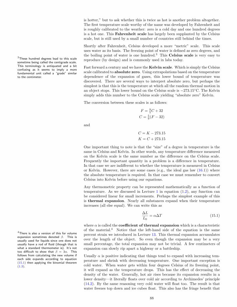
is hotter,” but to ask whether this is twice as hot is another problem altogether.The first temperature scale worthy of the name was developed by Fahrenheit andis roughly calibrated to the weather: zero is a cold day and one hundred degreesis a hot one. This Fahrenheit scale has largely been supplanted by the Celsiusscale, but is still used by a small number of countries still behind the times.

Shortly after Fahrenheit, Celsius developed a more “metric” scale. This scaleuses water as its basis. The freezing point of water is defined as zero degrees, andthe boiling point of water is one hundred.3 This Celsius scale is very easy to

3These hundred degrees lead to this scalesometime being called the centigrade scale.This terminology is antiquated and a bitconfusing as it seems to imply a morefundamental unit called a “grade” similarto the centimeter.

reproduce (by design) and is commonly used in labs today.

Fast forward a century and we have the Kelvin scale. Which is simply the Celsiusscale calibrated to absolute zero. Using extrapolations based on the temperaturedependence of the expansion of gases, this lower bound of temperature wasdiscovered. There are several ways to interpret absolute zero, but perhaps thesimplest is that this is the temperature at which all the random thermal motion inan object stops. This lower bound on the Celsius scale is −273.15C. The Kelvinsimply adds this number to the Celsius scale yielding “absolute zero” Kelvin.

The conversion between these scales is as follows:

F = 95C + 32

C = 59 (F − 32)

and

C = K − 273.15

K = C + 273.15

One important thing to note is that the “size” of a degree in temperature is thesame in Celsius and Kelvin. In other words, any temperature difference measuredon the Kelvin scale is the same number as the difference on the Celsius scale.Frequently the important quantity in a problem is a difference in temperature.In that case we are indifferent to whether the temperature is measured in Celsiusor Kelvin. However, there are some cases (e.g., the ideal gas law (16.1)) wherethe absolute temperature is required. In that case we must remember to convertCelsius into Kelvin before using our equations.

Any thermometric property can be represented mathematically as a function oftemperature. As we discussed in Lecture 1 in equation (1.2), any function canbe considered linear for small increments. Perhaps the simplest example of thisis thermal expansion. Nearly all substances expand when their temperatureincreases (all else equal). We can write this as

∆L

L0= α∆T (15.1)

where α is called the coefficient of thermal expansion which is a characteristicof the material.4 Notice that the left-hand side of the equation is the same

4There is also a version of this for volumeexpansion sometimes denoted β. This isusually used for liquids since one does notusually have a rod of fluid (though that iswhat a standard thermometer is). It’s nottoo difficult to show that β = 3α. Thisfollows from calculating the new volume ifeach side expands according to equation(15.1) then applying the binomial theorem(1.3).

percent strain we introduced in Lecture 13. This thermal expansion accumulatesover the length of the object. So even though the expansion may be a verysmall percentage, the total expansion may not be trivial. A few centimeters ofexpansion can slowly rip apart a highway or a battleship.

Usually α is positive indicating that things tend to expand with increasing tem-perature and shrink with decreasing temperature. One important exception iscold water. When water gets within four degrees Celsius of its freezing point,it will expand as the temperature drops. This has the effect of decreasing thedensity of the water. Generally, hot air rises because its expansion results in alower density—it literally floats over cold air according to Archimedes’ principle(14.2). By the same reasoning very cold water will float too. The result is thatwater freezes top down and ice cubes float. This also has the fringe benefit that

88

life can survive in a frozen-over lake because the ice acts as thermal insulationfor the liquid water below. One common downside is that frozen pipes burst forthe same reason. In fact, the freezing of water in rocks is a major contributor togeological erosion.

Having now established a way to quantify and measure temperature, we areprepared to discuss the flow of heat. Here is where we begin to create a distinctionbetween the ideas of temperature and heat. We see temperature differences asthe driver of heat flow.5 For any solid heat will flow via heat conduction. The

5Although it is tempting to think of temper-ature as a kind of potential energy creatinga force which drives the flow of heat, thisapproach doesn’t work. Essentially this isthe caloric fluid model of heat. There aretwo fundamental problems: (1) temperaturehas a natural lower bound, and (2) it isbetter to associate heat with energy ratherthan the temperature.

rate at which heat energy is transported (i.e., power) is given by

P =Q

t= k

A

L∆T (15.2)

where k is the thermal conductivity of the material. The larger the surfacearea A, the smaller the length L, the larger the temperature difference ∆T , theeasier heat will flow.6

6It should be noted that this is for the sim-plistic case of heat flowing straight througha rod. The conduction of heat throughmore complex geometries will obey differentequations.

This formula is similar in form to other equations describing flow like Fick’s law(16.5) and Ohm’s law (24.3). The opposite of conduction is resistance. Onequantity you may have seen before is the “R-value” which is defined as L/k.This metric is used rate the quality of insulation. Since it involves the reciprocalof thermal conductivity, this is a kind of thermal resistance. The better theinsulation, the higher the R-value. An R-value of 5.6 per inch (typical US homeinsulation) corresponds roughly to one in SI units.

Heat conduction also occurs in fluids, but heat convection completely washesout any effect. Convection is caused by the heat being carried with the fluid ratherthan through it. Since no mass transport occurs in solids, there is no convectionpossible, but with fluids it is the main method of heat transfer. Unfortunately,fluid flow is so complicated that there is no single formula to describe convection.

The third and final way in which heat moves is through heat radiation. Thisis heat transported through the electromagnetic field. This is the weakest formof heat flow, but will work in the vacuum of space and is how the sun warms theearth. The formula for heat radiation is

P =Q

t= eσAT 4 (15.3)

where e is called the emissivity and is a property of the material ranging fromzero to one. The value of σ is 5.67× 10−8 and is called the Stefan-Boltzmannconstant. It is a property of the electromagnetic field.7 The surface area of the

7I don’t see any reason to not also have heatradiation via the gravitational field. Thecorresponding constant would be minusculecompared to the electromagnetic field how-ever.

radiating object is A and T is its absolute temperature in Kelvin.8

8This is an example of one of the formulawhere it is important to use Kelvin ratherthan Celsius. The easy way to rememberwhich is that ∆T can be either Kelvin orCelsius, but just T must be Kelvin.

Heat will flow whenever there is a temperature differential. But this still doesnot completely explain what makes some things hot and others cold. As we pourheat into a substance different materials require more heat than others in orderto generate the same increase in temperature. This is called the heat capacityof the material. In general, we have:

Q = cm∆T (15.4)

where c is the heat capacity, m is the mass involved and Q is the total heat flowrequired for the ∆T change in temperature.

As we continue to pour heat into a solid object, it will eventually melt. While itis undergoing this phase change, the temperature remains constant. The heat isgoing somewhere, but not into an increase in temperature. If one were to plot thetemperature as a function of the heat input, the graph would flat-line here. Thisa characteristic of every phase transition. During the transition the substanceis a mixture of the two phases—each at the same temperature.9 A typical graph

9In fact, it is possible for all three phasesto coexist. This will only occur at aparticular combination of temperature andpressure and is called the triple point of thesubstance. In fact, the modern definitionof the Kelvin scale uses the triple point ofwater rather than the melting and boilingpoints originally used.

might look like Figure 15.2.

89

Figure 15.2: Typical phase change diagram

T

Q

Soli

d

Mel

tin

g

Liq

uid

Eva

por

atio

n

Gas

The slope on this graph represents the heat capacity of the substance. Thehorizontal distance during the phase changes represent the latent heat requiredto complete the phase transition. As such, each phase transition requires a certainamount of heat given by

Q = mL (15.5)

Each transition has its own L value. This makes it possible for us to solve a basiccalorimetry problem like the following.

Sometimes I make my coffee too hot, so I mix in a bit of ice to cool it down.Suppose I have 300 grams of coffee (which is basically water) at 80C and mix itwith 30 grams of ice at −10C. What is the final temperature of the mixture?

Let’s call the final temperature for which we are solving T . The amount of heatthat flows out of the coffee is given by

Q1 = (4186)(0.300)(T − 80)

because water has a specific heat of 4186. This heat flow will be negative becausethe coffee is losing heat.

The process for the ice is three-fold. First, its temperature needs to be broughtup the boiling point:

(2000)(0.030)(10) = 600

then it must melt:(335000)(0.030) = 10050

and then this melted ice must be brought to the final temperature T :

(4186)(0.030)(T − 0)

So the total heat that the ice absorbs is

Q2 = 10650 + (125.58)(T )

Since the all the heat lost from the coffee is gained by the ice (no “leakage” ofheat), the total change in heat is zero. Thus

Q1 +Q2 = 0

or(4186)(0.300)(T − 80) + 10650 + (125.58)(T ) = 0

Solving for T yields a final temperature of 65 degrees Celsius.

90

Gas

Liquid Solid

Con

dens

atio

nE

vapor

atio

n

Freezing

Melting

Sublimation

Dep

osition

Figure 15.3: The six possible phase transitions between threephases

For specific combinations of pressure and volume, transitions between any twophases is possible. Consider the diagram in Figure 15.3.

In fact, it is possible to have even more phase transitions. As an extreme example,plutonium has six different solid phases making it very difficult to work with.10

10See here for more details.Liquid helium has two different phases with a transition at 2.17 kelvin. Belowthat value it acts as a super-fluid with zero viscosity (something like how asuperconductor drops to zero resistance below a certain temperature—see below).

Finally, we will wrap up the lecture with a few notes on temperature extremes. Atthe hot end of the scale there is actually a fourth state of matter called plasma.This occurs when the random collisions between the atoms in a gas become soviolent that they literally tear the atoms apart into ions and electrons. Plasmasare used frequently in high-tech manufacturing processes and other industrialapplications.

But because plasma is electrically active, the fluid dynamics are extremely difficultto model. The currents of plasma have a tendency to curl and twist around oneanother and “pinch” in ways that make it difficult to control. This difficulty isone of the main obstacles in the creation of nuclear fusion energy.

On the other extreme is the very cold. One of the ways to cool down a gas is byletting it quickly expand—essentially reversing equation (15.1). In this way onecan create temperatures cold enough to liquefy air. This makes liquid nitrogenpretty easy to acquire for practical uses. Obviously its extremely cold temperaturecan make it dangerous if used improperly.

Getting closer and closer to absolute zero is quite a story in the history of physics.Each increment is more and more difficult to accomplish (like approaching thespeed of light). Along the way we find superconductivity. First discoveredin the early 1900s, this phenomena is when the resistance of certain metalsdrops to zero—not close to, but literally zero. This is one of the few quantummechanical effects on a macroscopic scale (the laser is another). As temperaturesdrop, these quantum mechanical effects become more evident in various ways.Superconductivity is one of the most dramatic examples of this.

Next week we will continue the story of heat and temperature. The focus will beon kinetic theory. By assuming that molecules in a gas interact via simple elasticcollisions, we will be able to derive the relationship between pressure, volume,and temperature for an ideal gas. This approach is called statistical mechanicsand involves quite a bit of math, so we will only be able to touch the surfaceof this subject. We will also see that diffusion can be explained using the samekinetic theory. In the end we will see that classical statistical mechanics is notas successful as it ought to be given the success of Newtonian mechanics. These

91

failures pave the way to the discovery of quantum mechanics which we will reviewin Lecture 22.

92

Lecture 16

Kinetic TheoryRead sections 14.1–14.4, review Lecture 8

In the previous lecture we investigated some of the basic properties of heat andtemperature by focusing on what heat “does”: how to measure it, how it flows,etc. In this lecture we focus on what heat “is”: the random motion of molecules.

Richard Feynman has said,

If, in some cataclysm, all of scientific knowledge were to be destroyed,and only one sentence passed on to the next generation of creatures,what statement would contain the most information in the fewestwords? I believe it is the atomic hypothesis that

All things are made of atoms—little particles that that move around inperpetual motion, attracting each other when they are a little distanceapart, but repelling upon being squeezed into one another.

In that one sentence, you will see, there is an enormous amount ofinformation about the world, if just a little imagination and thinkingare applied.

Well, today we will apply this idea in the context of the kinetic theory of gases.The basic idea is that the higher the temperature of a gas, the more kineticenergy the molecules possess. We can even incorporate phase changes into thisframework by associating latent heat with the potential energy created throughinter-molecular interactions.1

1A truly phenomenal website with a simplemolecular dynamics applet is located here.Before we can speak in detail about molecular motion we need to deal with their

size. The radius of a typical atom is on the order of the nanometer. This meansthat the number of atoms in any laboratory sample is huge. It also means thatthey are essentially unobservable without highly specialized equipment. This wasa major obstacle for the adoption of the atomic hypothesis in the early 1900s.It was none other than Albert Einstein who analyzed Brownian motion (therandom, jerky motion of particulates suspended in a fluid) that provided the firstindisputable physical evidence for the atom.

The point here is that the fundamental unit of the mole2 has been developed to2Abbreviation: mol. I believe that this issimply a shortening of the word molecule.

deal with this atomic size. By definition, the mole is the number of atoms in 12grams of carbon-12 (a specific isotope of carbon—see Lecture 29) and has a valueof 6.022× 1023. This number is called Avagadro’s number labeled NA.

You may wonder why we need a special unit for something that is just a number.Isn’t it just a naming convention, like a dozen eggs? In a fundamental sense thatis true, but one must remember that we are human. No matter how sophisticatedour machinery becomes, ultimately measurements must be translated to and from

93

this human scale. There is no way to literally count the number of atoms in aparticular sample.3 In other words, the mole is not just a number that we simply

3Maybe with the advances in nanotechnol-ogy this will be possible. If that day evercomes, we will still need to define the count-ing process in a way that is reproducible andindependent of external variables.

arbitrarily choose—it represents the relationship between the lab and the atomicworld. This relationship is best summarized in the following formula:

grams

mole=

molecular mass

molecule

where the molecular mass is the mass of each molecule in so called atomicmass units. By definition a carbon-12 atom has a mass of 12 amu. The atomicmass units are listed in any periodic chart, so given the chemical make-up of asubstance we can determine its total molecular mass and therefore the number ofmoles in a particular sample.

With this link back to the lab we are now prepared to dive into the world of themicroscopic. The simplest microscopic system to analyze is an ideal gas. In anideal gas, we assume that the molecules have two properties.

• Negligible interaction (which will eliminate any possible phase transitions)

• Negligible size (which will allow the volume to decrease without limit)

We relax both of these conditions enough to allow the molecules to interactthrough elastic collisions. These collisions will be the only mechanism to distributekinetic energy throughout the gas (other than collision with the walls of thecontainer). Most gases at standard temperature and pressure4 can be considered

4Most commonly 0C and 101.3 kPa (at-mospheric pressure), though some organi-zations use different definitions.

ideal.

As mentioned in the previous lecture, gases will expand with increasing temper-ature. This volume is obviously also related to the pressure surrounding the gas.These three variables combine in the ideal gas law

PV = nRT (16.1)

where n is the number of moles of gas and R is a proportionality constant equalto 8.31 in SI units. An alternate form is

PV = NkT (16.2)

where N represents the number of molecules in the gas and k = R/NA is calledthe Boltzmann constant.

Now we are ready to introduce some mechanics. Consider a single particle trappedin a cubical box of length L. Suppose the particle moves parallel with one of theedges of the box—we will call this direction x. Assuming the atom strikes andrebounds off the way elastically (this is an ideal gas), the change in momentumis given by

∆p = 2mv

This collision will occur every time the atom travels the length of the box twice.Given the velocity v, we have

∆t = 2L/v

Combining these two results according to the impulse form of Newton’s law (8.2)gives us an average force per collision5 of

5This calculation is similar to the “machinegun pressure” problem in Lecture 8 on page44.

〈F 〉 = mv2/L

Since pressure is average force over area, we may write

PV = mv2

The right-hand side is simply twice the kinetic energy of the atom.

94

Now if we consider a random collection of molecules, the momentum will be splitinto three due to the three dimension of space, so in general we have

PV = 23N〈KE〉

where 〈KE〉 represents the average kinetic energy per molecule. Comparing thiswith 16.2 yields

〈KE〉 = 32kT (16.3)

which explicitly shows the relationship between the temperature of the gas andthe random motion of its molecules. This average motion is called the internalenergy of the gas. Its the kinetic energy of the system after the bulk motion hasbeen isolated. We have shown the internal energy of an ideal gas to be 3

2NkT or32nRT .

The above derivation of the internal energy of an ideal gas is an example of the useof statistical mechanics. Essentially we assume that our system is composed ofa large number of identical pieces (atoms). By applying the laws of mechanics toeach part, we can take the overall average to derive the properties of the overallsystem. For example, if we relax our restrictions on an ideal gas a bit we canderive the Van der Walls equation:(

P + an2

V 2

)(V − nb) = nRT (16.4)

where a is related to the attraction between the molecules and b the “size” of themolecules. This represents an improvement over the ideal gas law (16.1) and isapplicable to liquids as well.

Derivations can go the other way too. The Maxwell-Boltzmann distributionrepresents the number of molecules at various speeds in the gas. There are severalsimulators on the web to show how this distribution works (here’s one: hit setupthen go, use the slider to slow down the animation). The point is that even ifthe molecules all start with the same speed, through random collisions some willincrease in speed and some will decrease. The distribution of speeds over the longhaul is what the Maxwell-Boltzmann distribution describes.

An example of the distribution is given in Figure 16.1. One thing to note isthat although the average speed does increases with temperature, there is alwaysa range to the speeds: there are always some that are slow and some that arefast. This is one of the ways to explain evaporation. No matter what the overalltemperature of the liquid, there will always be some molecules with high kineticenergies. These molecules have enough energy to escape the potential well thatbinds the liquid together and escape.

Molecular speed

Nu

mb

erof

mol

ecu

les

Low T

High T

Figure 16.1: Example of the Maxwell-Boltzmann distributionof speeds in an ideal gas.

On the technical side, notice that the distribution is not symmetric (no negativevalues). This implies that the most probable speed (the peak of the graph) is notthe same as the average speed. It can be shown that the average is about 13%larger than the peak value.

95

In fact, the distribution of the kinetic energies depends on v2, so the shape isdifferent though qualitatively the same. But the average kinetic energy does notcorrespond to either the most probable speed or the average speed. The speedto which it does correspond is called the root-mean-square (abbreviated asRMS) because it is the square root of the average of the square of the speeds.This complicated sounding calculation is actually quite common and shows up in avariety of contexts related to statistics. Usually called the standard deviation6,

6Actually, for technical reasons the defini-tion of standard deviation is not quite thesame as root-mean-square.

it is a good measure of the distribution in the variable of interest. One way to seethis is that the straight average will cancel negative and positive contributions(which gets you to the middle), but the root-mean-square will accumulate them(which gets at the spread of values). For the Maxwell-Boltzmann distribution,the RMS speed is about 22% larger than the peak value.

Diffusion is the process in which solutes flow from regions of high concentrationto low concentration. The substrate through which the flow occurs could be solid,liquid or gaseous. Diffusion is comparable to heat conduction in many ways and iseasy to understand using kinetic theory. Some of the molecules on the boundaryof the high concentration region will have a random motion away from that region.As these molecules flow away they reach the area of low concentration. Thoughmolecules are leaving the low concentration area also, they do so at a smaller rate.More flow in than out. Eventually a concentration equilibrium is established andthere is not net flow of material (though the individual molecules are constantlymoving back and forth).

The equation governing diffusion is Fick’s law:

M

t= D

A

L∆C (16.5)

Notice the similarity to the equation for thermal conduction (15.2). The amountof mass M transported per second is proportional to the concentration differential∆C, the geometry of the situation A/L, and a proportionality constant D calledthe diffusion constant.

This is the basic process behind osmosis which has so many applications inbiology. The osmotic pressure due to the concentration differentials in water isresponsible for the rigidity of plants, the stability of the cell, and is how plantsdraw water and nutrients from the soil.

Diffusion is also used in many high-tech processes to control the electrical prop-erties of various substances. We will talk about some of these applications inLecture 28.

It is easy to take the success of kinetic theory for granted. For over two centuriesthe applications of Newtonian mechanics continued to spread until some beganto think there was no other way the universe could work. They were wrong andthe first signs were discovered in the decades prior to and after 1900. Of thetwo scientific “revolutions” around this time, the changes wrought by quantummechanics exceed that of relativity. When viewed the right way, relativity can beseen as a tweak to the framework of Newtonian mechanics—quantum mechanicsreworks the very conceptual foundation. We will return to this topic in Lecture 22and discuss relativity and quantum mechanics in more detail in Lectures 26 and27. But for now it is worth mentioning some of the cracks that were discoveredin this foundation related to kinetic theory.

The first crack we have already mentioned: superconductivity. As temperaturesget down near absolute zero, the electrical resistance of certain materials dropto zero. We shouldn’t be surprised to find that electrical resistance drops withdecreasing temperature, but exactly zero implies new physics.

The second crack is the heat capacity of solids. According to kinetic theory theheat capacity of any solid should be 3R. This is based on a result from statisticalmechanics called the equipartition principle. It states that the internal energy

96

of a system in thermal equilibrium is 12kT for each degree of freedom. We have

seen an example of this in equation (16.3)—the particle has three degrees offreedom corresponding to the three dimensions of motion. In fact, the internalenergy of a diatomic molecule is 7

2kT per molecule because it has seven degreesof freedom.7

7Three for translation, two for rotation, andtwo for vibration. There are only two fortranslation because rotation about the axisthat connects the two atoms is no motion atall (symmetry). Two for vibration becausethe energy has both kinetic and potentialmodes.

For atoms locked in a solid, there is no translation or rotation, but they canvibrate in three dimensions which means that there are six degrees of freedom permolecule, so the internal energy of the solid ought to be 3NkT which correspondsto a specific heat capacity of 3R. However, as temperatures get cold the heatcapacity of a real solid drops. It is as if some of the degrees of freedom are getting“frozen” out.8 This is purely quantum mechanical effect. Einstein created the

8In fact, a typical diatomic gas (like nitro-gen or oxygen) actually has a specific heatcapacity closer to 2.5 because the vibra-tional modes are inactive. More complexmolecules are locked down to about 3. Seehere.

first quantum model that correctly predicted this effect.

The third crack involves something called the ultraviolet catastrophe. Histor-ically, this is the start of all things quantum. This problem is related to the heatradiation from a so-called blackbody, or an object with emissivity equal to one.The energy spectrum from a black body is qualitatively like that of the distribu-tion in Figure 16.1,9 but classical statistical mechanics predicts the spectrum to

9I’m just too lazy to draw anotherdiagram—the equations are different. SeeFigure 22.1 for an accurate picture.

extend into the low wavelength (ultraviolet) without limit. This would imply thatall radiation should occur beyond the visible spectrum which anyone who has satin front of a campfire would say is clearly nonsense. Interestingly, Einstein alsohad a role to play in recognizing the way that the quantum hypothesis (introducedby Planck) could resolve this embarrassment.

Next week we will finish off our discussion of heat and temperature by talkingabout thermodynamics proper. This can be seen as a continuation of Lecture 15,but we will need our calculations of internal energy (16.3) to complete the picture.We will state and discuss the laws of thermodynamics, the first of which is simplythe conservation of energy. Using simplified thermodynamic processes we will talkabout efficiency in heat engines which will lead us to discuss reversibility. Thisin turn will motivate the definition of a new quantity called entropy which is thesubject of the (infamous) second law of thermodynamics.

97

98

Lecture 17

ThermodynamicsRead sections 15.3–15.12

The science of thermodynamics is a product of the industrial revolution and thepursuit of a more efficient steam engine. As such the approach has a strongengineering emphasis—practical rather than theoretical. Another way in whichit is distinguished from mechanics is that the approach has more “systems”reasoning: we focus on how the properties of the systems interact and change.Though statistical mechanics sheds much light on thermodynamics, technicallythey are independent. As such, the laws of thermodynamics are is still valid whenquantum mechanics replaces classical mechanics.

Our starting point is the conservation of energy. This is called the first law ofthermodynamics and is usually written as

∆U = Q−W (17.1)

Basically this is saying two things:

• Heating a system increases its internal energy (∆U = Q).

• Work done by a system decreases its internal energy (∆U = −W ).

Equation (17.1) is written in the context of heat engines, so the concern is howmuch work we can get out of the system—which is why there is a negative signin front of W .

Remember that the internal energy of a system is directly related to its temper-ature. For an ideal gas we have

∆U = dkT/2

where d is the number of degrees of freedom for the molecule—we will assumed = 3 for a monatomic gas (like argon) and d = 5 for a diatomic gas (like oxygen)(see page ??).

The first law doesn’t seem to say much until we start to add some informationabout the system under consideration. The simplest system to consider is an idealgas, for which we have the ideal gas law (16.1). There are four basic parametersinvolved: pressure, volume, amount of material (moles), and temperature. Thefirst two are related to work through W = P∆V .1

1This follows from the definition of workW = F∆x. Divide the first factor by A toget pressure and multiply it into the secondfactor to get V .

We will normally assume the amount of material is constant in a particularprocess. However, the other three variables may change in various ways. We willfocus on four simpler processes each of which hold a particular variable constant.

99

The first process is isothermal, meaning that the temperature is held constant.A common way to do this is to connect the system to a heat reservoir.2 This

2Sometimes called a “heat bath”. is simply an outside system which is considered so large that the change in itstemperature is negligible due to the flow of heat to and from our system of interest.

Since the temperature is held constant, we know two things. First, the change ininternal energy is zero. Second, from the ideal gas law we know that the product ofpressure and volume is constant. Usually in an engine we manipulate the volume(driving a piston, for example), so we are interested in the work done when thevolume changes in the gas. The challenge here is that the pressure changes too.This calculation involves a bit of calculus, so I will simply quote the result:

Wisoth = nRT ln(V/V0) (17.2)

A volume increase corresponds to positive work. Since the temperature is heldconstant, heat must be flowing into the system from the reservoir to support theprocess. The amount of heat is equal to the work done according to the first law.This isothermal process shows that it is possible to manipulate the flow of heatwithout a temperature differential.

The second process to consider is isobaric, meaning that the pressure is heldconstant. In this case, the ideal gas law tells us that ratio of volume andtemperature is constant. The work done is simply Wisoba = P∆V because thepressure is constant. An easy way to support this kind of process is through anopen container exposed to the atmosphere.

The third process is one with constant volume, like with a closed container. Thisis called a isochoric process. There is no work involved since ∆V = 0.

The fourth and final process we will consider is called adiabatic which means noheat flow. A thermally insulated container will obviously be adiabatic, but alsoany process that happens quickly. If the process is fast enough, there simply isnot enough time for the heat to flow. So, whether a given process is adiabaticor not depends on the thermal conductivity of the materials. But if there is noheat flow, the first law reduces to ∆U = −W , so the work done in an adiabaticprocess comes from the internal energy of the gas (and a corresponding decreasein temperature). We have:

Wadiab = − 32nR∆T (17.3)

for a monatomic ideal gas.

In a way, the adiabatic process stands in contrast to the isothermal process. Bothinvolve divorcing the connection between heat and temperature. In the adia-batic flow temperature changes without heat flow but in this isothermal processheat flows without a temperature change. The connection between pressure andvolume is similar too. For an adiabatic process we have

PV γ = constant (17.4)

where γ is a number larger than one.3 For an ideal gas, we have3It can be shown that this γ is equal tothe ratio of the specific heat capacity of thegas at constant pressure relative to that atconstant volume.

γ =d+ 2

d

where d is the number of degrees of freedom. For the monatomic ideal gas,γ = 5/3. This shows that under compression the pressure in an adiabatic processwill rise faster than in an isothermal one. Under expansion the adiabatic pressurewill fall faster.

These four processes show us how it is possible to use the first law (17.1) toconvert heat flow into usable mechanical work. Any contraption that harnessesheat flow to create work is called a heat engine. Thermodynamics is primarily

100

the mathematics behind heat engines. Every heat engine is rated by its efficiencywhich is the power it generates in useful work divided by the power it consumes.4

4I like to draw a distinction between a ma-chine which multiplies force, and an enginewhich does work. In my mind the key metricfor a machine is its mechanical advantage,but for an engine it is power: how fast itcreates energy. I try and keep a distinctionin the nomenclature although I don’t thinkmost authors do.

This is equivalent to the definition we used in Lecture 7 of total work done overthe energy consumed because power is work per second.

Since a heat engine converts heat flow into work its primary waste product willbe heat energy. Since energy is conserved, we have a simple relationship

Qin = W +Qout

which simply says that the energy going in either comes out as usable work orwasted heat. This allows us to write a formula for efficiency in terms of heat:

e = 1− Qout

Qin(17.5)

So efficiency is the opposite of how much energy is wasted per unit of input energy.

With much fanfare, we are now ready to introduce the second law of thermo-dynamics:

Between high and low temperature, heat will flow spontaneously

Truly an inspiring statement, huh? I think the reason why there is so much talkabout the second law is that this sentence is a Trojan horse of sorts. This simple,obvious statement is the reason why no heat engine will ever be close to 100%efficient, why no perpetual motion machine can exist, and can even explain theultimate “heat death” of the universe. Understanding how this can be has leadto many alternate formulations of this law. We will discover a few along our way.

The key word in the previous statement is “spontaneously” which is closely relatedto irreversibility. Heat will not flow spontaneously from cold to hot. Of course,heat can flow against a temperature differential (this is what a refrigerator doesafter all). But when the heat flow is spontaneous, the system does not controlthe flow of energy. This is unlike a mechanical system in which the energy isflowing due to the internal forces between the parts. The mechanical energydistribution is directly related to the configuration of the system, so it is possible(in principle) to reverse the flow of energy by simply reverting this configurationback to its initial state. There is nothing a mechanical system can do to reversethe spontaneous flow of heat.

So spontaneous heat flow is bad for efficiency. We will now see that even aperfectly reversible heat engine cannot be 100% efficient. A heat engine requiresthe flow of heat. But the second law implies that only isothermal heat flow isreversible. In addition, any engine must cycle: the process must repeat. Thesimplest engine we can consider is one that uses an ideal gas (we’ve alreadycalculated the work involved for all four basic processes). A complete cyclewill involve returning to the same pressure, volume, and temperature. In fact,it’s sufficient to track just pressure and volume since if they match, so will thetemperature. We can plot the process on a PV -chart like Figure 17.1.

P

V

A

B

Figure 17.1: An isothermal process for anideal gas plotted on PV chart

Simply using isothermal processes is not enough for our engine, however. Wecould create a cycle from A to B and back, for example, but the work done inthe expansion process—given by equation (17.2)—is equal to the work requiredto compress the gas back to its initial state. We have an engine but it does nonet work.

We can do better. An adiabatic process is also reversible because there is no heatflow at all. This will give us a way to change the temperature of the gas. Thesimplest non-trivial process which combines isothermal and adiabatic processes iscalled a Carnot cycle (see Figure 17.2).

V

P

1

2

3

4

Figure 17.2: Example of the Carnot re-versible cycle for a monatomic ideal gas

101

Suppose we start the ideal gas in a state of high pressure and low volume. Thefirst step is isothermal expansion. For example, we allow the gas to expand whilethermally connected to a heat reservoir at temperature T1. The work done by thegas is given by equation (17.2). The second step is adiabatic expansion. We nowdisconnect the gas from the heat reservoir, thermally isolate the gas, and allow itto continue to expand. The work the gas does is given by (17.3). The gas is nowin a low pressure, high volume state with a temperature lower than the initialstate.

This is all the work we are going to get out of the engine. We now need to workon returning the gas back to it original state (high pressure, low volume) in orderto complete the cycle so we need to compress it. Adiabatic compression willsimply reverse what we have already done, so the third step should be isothermalcompression. Thermally connect the gas to another heat reservoir at temperatureT2 and compress it.5 The fourth step is adiabatic compression which will bring

5How far should we compress it? It takesa bit of calculation, but we need VD/VC =VA/VB . This will cause the fourth step toactually complete the cycle.

the gas back to its original state.

Work is required in the last two steps, but it will be less than the work done bythe gas.6 We know that the efficiency of the engine is the net work done divided

6The net work is actually the area enclosedwithin the curve from Figure 17.2.

by the input heat energy. This input heat energy occurs during the isothermalexpansion. The amount of heat is given by equation (17.2) because of the firstlaw and the fact that the internal energy does not change.

The heat wasted occurs during the isothermal compression and is also given by(17.2). Putting all of these facts together gives us the efficiency for our engine:

e = 1− Tcold

Thot(17.6)

Here’s the kicker (and also the insight that put Carnot in the history books). Thisis the best any heat engine can do between reservoirs of these two temperatures.The argument has two parts. The first is simply that any irreversible enginewill have a lower efficiency than a reversible one. This is pretty obvious as anyspontaneous heat flow will simply add to the wasted heat without any productivework. The second is that every reversible engine will have the same efficiency.One way to see this is by supposing we have two reversible engines with differentefficiencies. Since they are truly reversible, run the more efficient one backwardby using the work generated from the first one. In this way we generate excesswork without any net heat flow at all!

So, although equation (17.6) was derived for an ideal gas, it represent the maxi-mum possible efficiency of any heat engine. Obviously a real heat engine will beworse.

Take a moment to compare (17.6) with (17.5). They allow us to write

Qhot

Thot=Qcold

Tcold

for the Carnot cycle we have been discussing. This suggests there is a kind ofquality of heat flow at various temperatures. In a way, the quality of heat flowat a lower temperature is greater than at a higher temperature. This “quality” isrelated to reversibility and is not called entropy.

Entropy is a way of grading the internal energy of a system and is closely relatedto how closely the system is to thermal equilibrium. When the internal energyof a system is far from equilibrium, it is said to be in a low entropy state. Forexample, when one hot and one cold object are thermally connected (forming onesystem) heat will flow. In other words, the internal energy of the combined systemredistributes itself until it reaches thermal equilibrium (uniform temperature).Another way to say this is that the system moves from a low to a high entropystate.

102

Whenever heat flows out of a system, the entropy changes by

∆S =Q

T(17.7)

where S represents the entropy of the system.7 By this definition, the entropy7This formula only works for an reversibleisothermal process. In order to calculatethe entropy change for an arbitrary process,it is sufficient to do so for another processthat connects the beginning and end states.The entropy change is independent of theprocess used to get there.

change in the Carnot cycle is zero. In this way the change in entropy representsthe “quality” of the heat flow. In an irreversible cycle, the entropy created whenthe heat flows out of the system at the low temperature exceeds the reductionthat occurs when heat is absorbed at the high temperature. The net entropychange is positive. This is a characteristic of any irreversible cycle.

Entropy is a recognition of the fact that internal energy tends to uniformity. Inthis way, the second law of thermodynamics is often written as

∆S ≥ 0 (17.8)

Be aware what this statement does not say: it does not say entropy neverdecreases—it often does. But whenever the internal energy of a system is pushedaway from thermal equilibrium, the entropy increases in the external environmentthat is doing the pushing. At best the total entropy (system plus surroundings)is zero for a reversible process. The total entropy increases for an irreversibleprocess. Every decrease in entropy is accompanied by a larger increase in entropysomewhere else.8

8There is a small loophole here. Anotherway to affect the entropy of a system isby combining it with another: the totalentropy is the sum of the two parts. Ifthe absolute entropy of a system could everbe negative, we could reduce the total inthis way. The so-called third law of ther-modynamics closes this loophole by statingthat the entropy of a system is only zero atabsolute zero. In this way, the entropy of asystem can never be made negative.

The heat flow that occurs into the cold reservoir is wasted energy and is lost formechanical work. The entropy change of the process offers us a way to quantifythis through the formula

Wlost = T0∆S (17.9)

where T0 is the temperature of the coldest reservoir in the system.

We are now prepared to come full circle and discuss entropy in the context ofkinetic theory. I have already mentioned how entropy represents the distributionof the energy in a system. For example, if we take a system and divide into twoparts, the energy distribution will follow the degrees of freedom in the system.

We define the microscopic state our system as the way in which the energy isdistributed. It can be shown that the number of states available to a system isexponentially dependent upon its degrees of freedom:

Ω ∝ Ed/2 (17.10)

Since the degrees of freedom of a typical gas is related to the number of its atoms,this can become a very large number. The number of ways in which the energycan be distributed uniformly far outnumber the other ways it can be distributed.

A simple example calculation is shown in Table 17.1 for a system with five unitsof energy. The system has two parts with six and four degrees of freedom in thefirst and second parts, respectively. Notice how the largest number of total statesoccurs when the energy per degree of freedom is equal in the two parts. Increasingthe degrees of freedom makes the distribution much more extreme.

E1 E2 Ω1 Ω2 Ω

0 5 0 25 0

1 4 1 16 16

2 3 8 9 72

3 2 27 4 108

4 1 64 1 64

5 0 125 0 0

Table 17.1: Calculation of the number ofstates in a simple two-part system

The basic postulate of kinetic theory in this context is that the probability ofthe system being in any microscopic state is equal. In effect this means that thesystem is usually in a state of uniform distribution. The system is constantlybouncing between different states, but there are so many that the effect is topull the system to uniformity—which we have previously called equilibrium and“explains” the second law.

Boltzman was able to show that the absolute entropy of a system is related tothe number of states by

S = k ln Ω (17.11)

103

a result of which he was so proud that he has it engraved on his tombstone.

This completes our survey of thermodynamics. We will switch gears again todiscuss wave motion. This will occupy us for the next couple of lectures and thenwe will apply some of these results to the study of sound and light. In the firstlecture we will discuss how waves are generated from a single source. The primaryeffect is the radiation of energy through some medium whether it is a string, theair, or the electromagnetic field. The speed, wavelength, and intensity of the wavewill be discussed. We will extend the topic a bit to include multiple sources atthe same location. In the lecture after we will discuss multiple sources separatedin space (which leads to interference—the chief characteristic of waves.).

104

Lecture 18

Wave Motion and RadiationRead sections 16.1–16.9

Radiation can be divided into two classes: that which transports mass and thatwhich transports energy. An example of the first class is nuclear radiation. Whennuclear energy is released, each atomic nucleus acts like a little bomb. The atomicparticles go flying in all directions carrying residual kinetic energy. This atomicshrapnel we call radiation. We will see in Lecture 29 that there are three typesof natural nuclear radiation each with varying properties.

The second class of radiation is that which transports only energy. This is thekind we refer to when a pebble is dropped in a still pond and we say that theripples radiate from the impact. This radiation does real work—each wave erodesthe shoreline a tiny bit—so energy is truly being transported.

In the first case, the radiation is simply mass in motion. This mass carriesmomentum and energy which interacts with other matter through the principleswe have already studied. But the second case is different. No mass moves frompoint A to point B, only energy. This energy transport requires a wave medium.The medium does not itself move from point A to point B, but it does supportthis transmission of energy.

In order to support this transmission of energy, the medium must be composed ofinterconnected parts.1 There are many different types of media: strings are the

1This interconnection is the crucial ingredi-ent and makes the wave motion possible—when one particle moves, those connectedwill be dragged along with it. These in turnwill drag additional parts which propagatesthe disturbance through the entire medium.

simplest model, but we will also talk about the way waves move through solidsand fluids. The electromagnetic field also acts as a medium for waves, althoughit is a bit of a special case (we will revisit this issue in Lecture 21 and 22).

Since the applications of wave motion are so wide spread, it is useful to keepthe discussion fairly abstract. However, most wave phenomena can be seen ina simple string. The essential characteristic of the wave medium is that it becomposed of coupled oscillators all near equilibrium.

Although the medium itself does not move in bulk, there is a direction involved inthe radiation of energy. We say that we have a transverse wave if the oscillationin the medium is perpendicular to the movement of the disturbance (like a string).We have a longitudinal wave if the oscillation is parallel to the radiation (likea compressed spring, or sound waves). Wave motion is not confined to either/or:typical water waves have both transverse and longitudinal components.

By definition, the disturbance of a transverse wave has only one degree of freedom,but a longitudinal wave has two (the y and the z if it is moving along the x-direction). To completely describe the wave we need to specify its direction. Thisis called the polarization of the wave.2 In addition, the disturbance need not

2It is a bit more complicated than this sincewe could drive the string with a circulartype of motion. In that case, the directionof the oscillation rotates in time: this iscalled circular polarization. More complexcombinations are possible as well.

be a physical displacement. We could speak of a heat wave, for example. As long

105

as the medium is coupled across this property, radiation will occur. The possiblepolarization states depend on the nature of the medium.

Because we are essentially discussing the motion of oscillators, the mathematicsbegins where Lecture 12 left off. The basic result was that when a system isoscillating sufficiently near equilibrium, the oscillation is governed by equation(12.5). However, our oscillators are connected to one another, and the radiationhas a dampening effect as the energy is propagated away.3 The oscillation of each

3The rate at which this energy is car-ried away is called the impedance of themedium.

element in the medium looks more like Figure 12.5.

Now instead of focusing on each element in the medium, we want to discuss theprofile of the disturbance across the medium. For simplicity we will talk about anstring with a linear mass density of µ under tension T . An element of the stringwill experience a net force when it and its two neighbors are not in a straightline (see Figure 18.1). The net force due to the curvature in the string acts toeliminate that curvature. In fact, the stronger the curvature in that “line”, thegreater force of restoration. Mathematically, when the forces of restoration areproportional to the curvature of the disturbance, the medium obeys the waveequation and will support the kinds of waves we are discussing in this lecture.

TTa

Figure 18.1: Forces on the element of astring eliminate curvature

The speed with which any disturbance propagates through this string is alsorelated to the tension and linear mass density. For an ideal string, the speed isgiven by

v =√T/µ (18.1)

For a solid this speed represents the speed of sound in the substance. We have

v =√Y/ρ (18.2)

Actually, this is only the formula for a compression wave in a solid. When a solidis disturbed, the strain can propagate through shear stress as well.4 For a liquid

4In fact, this is an example of a non-standard polarization and is important inthe investigation of earthquakes. The twotypes of waves have different wave speedsand can be used to investigate the natureof the Earth’s core (see here for details).

we havev =

√B/ρ (18.3)

where B is the bulk modulus. Since the pressure in a gas is temperature depen-dent, so is the speed of sound. We have

v =√γkT/m (18.4)

where m represents the molecular mass of the gas.55A quick cheat for the speed of sound inair is v = 331 + 0.6Tcel where Tcel is thetemperature measured in Celsius. This canbe derived from equation (18.4) and thebinomial theorem (1.3).

If we pluck a string, the oscillation will eventually die away as the energy isradiated through the string (assuming the string is infinite in length). In orderto maintain a sustained wave pattern, we must have a source that supplies theenergy that is being drained away. The simplest driver is simply one that moveswith simple harmonic motion. As we discussed in Lecture 12, when an oscillator isdriven by an outside source, its frequency will match the frequency of the driverregardless of its natural frequency. In this way we can control the motion ofthe medium from this single driver: all the other elements of the medium (thatparticipate in the radiation) will vibrate with this same frequency.

If we consider a string that is being driven at one end by a simple harmonicoscillator, then the resulting disturbance will look like Figure 18.2. In this figurethe wave is traveling to the right. Notice how each element of the string oscillateswith the same frequency (the white dots, for example) as the driver on the farleft. If the motion of the element matches the driver, it is said to be in phase(the gray dots are in phase). If the motion is the exact opposite (when one is upthe other is down—like the white dot), it is said to be out of phase.

t=0

t=1

t=2

t=3

t=4

t=5

t=6

t=7

t=8

Figure 18.2: Sine wave profile over time

It is no coincidence that we use same word “phase” in this context and in equation(12.5). Consider the driver located at point x = 0. The closest element that is inphase with it (the first gray dot) has a phase shift of φ = −2π radians, since it isa full cycle behind the driver. The distance between these two elements is called

106

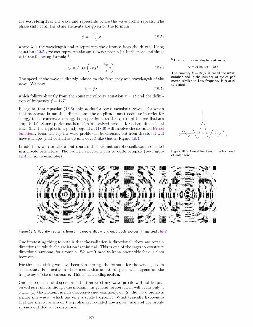
the wavelength of the wave and represents where the wave profile repeats. Thephase shift of all the other elements are given by the formula

φ = −2π

λx (18.5)

where λ is the wavelength and x represents the distance from the driver. Usingequation (12.5), we can represent the entire wave profile (in both space and time)with the following formula:6

6This formula can also be written as

ψ = A cos(ωt− kx)

The quantity k = 2π/λ is called the wavenumber and is the number of cycles permeter, similar to how frequency is relatedto period.

ψ = A cos

(2πft− 2π

λx

)(18.6)

The speed of the wave is directly related to the frequency and wavelength of thewave. We have

v = fλ (18.7)

which follows directly from the constant velocity equation x = vt and the defini-tion of frequency f = 1/T .

Recognize that equation (18.6) only works for one-dimensional waves. For wavesthat propagate in multiple dimensions, the amplitude must decrease in order forenergy to be conserved (energy is proportional to the square of the oscillation’samplitude). Some special mathematics is involved here . . . for a two-dimensionalwave (like the ripples in a pond), equation (18.6) will involve the so-called Besselfunctions. From the top the wave profile will be circular, but from the side it willhave a shape (that oscillates up and down) like that in Figure 18.3.

Figure 18.3: Bessel function of the first kindof order zero

In addition, we can talk about sources that are not simple oscillators: so-calledmultipole oscillators. The radiation patterns can be quite complex (see Figure18.4 for some examples).

Figure 18.4: Radiation patterns from a monopole, dipole, and quadrupole sources (image credit here)

One interesting thing to note is that the radiation is directional: there are certaindirections in which the radiation is minimal. This is one of the ways to constructdirectional antenna, for example. We won’t need to know about this for our classhowever.

For the ideal string we have been considering, the formula for the wave speed isa constant. Frequently in other media this radiation speed will depend on thefrequency of the disturbance. This is called dispersion.

One consequence of dispersion is that an arbitrary wave profile will not be pre-served as it moves though the medium. In general, preservation will occur only ifeither (1) the medium is non-dispersive (not common), or (2) the wave profile isa pure sine wave—which has only a single frequency. What typically happens isthat the sharp corners on the profile get rounded down over time and the profilespreads out due to its dispersion.

107

One final topic is required in this discussion of the radiation of wave energy:that of intensity. When we talk about sound and light as wave phenomena, theintensity corresponds to the our sensory perceptions of loudness and brightness(pitch and color correspond to the frequency of the wave). Physically, we definethe intensity of a wave as the power that passes through a certain area dividedby that area—a kind of density of how the power radiated.7 For a single point

7Actually, the intensity is closely relatedto the energy density of the field. Therelationship is I = ev, where e is the densityof energy (both potential and kinetic) andv is the speed of the radiation. We will seethis again in Lecture 26.

source, the intensity is related to the distance from the source by

I =P

4πr2(18.8)

The intensity drops with an inverse square law because the surface area of thesurrounding sphere increases with the square of the distance.

An important thing to note (for the next lecture) is that intensity is proportionalto the square of the amplitude of the wave since the energy depends on theamplitude squared as in equation (12.9).

However, this definition of intensity does not quite complete the story. Both thesensation of sound and light are not linear—the ear and eye are more sensitive tolower intensities than higher intensities. This suggests creating an alternate scaleto measure intensity called the intensity level and is measured in decibels. Theformula for decibel level is

β = 10 log(I/10−12) (18.9)

Although this scale could be used for light, it is designed to work for sound. Thisis because the sound intensity of 10−12 watts is the typical the threshold ofhearing. This formula calibrates the decibel level at the threshold of hearing tozero. Every decibel increase corresponds to a ten-fold increase in power.

Frequently we need to convert from decibels to intensity. This is done withlogarithms, but a short-cut involves using the inverse of the previous formula:

I = 100.1β−12 (18.10)

Next week we continue our discussion of wave motion. We investigate the mathe-matics of the interference of two waves and what it depends upon. We will also seethat waves can rebound off of a boundary (reflection) and can interfere with theoriginal wave source. For just the right combination, the incoming and reflectedwaves can combine to create a so-called standing wave. We will finish the topicby touching on the question of how waves of differing frequency interact.

108

Lecture 19

Wave Motion andInterferenceRead sections 17.1–17.7

Having discussed the way in which waves propagate through a medium in the lastlecture, we are now prepared to discuss how waves interact. Each wave emanatesfrom a source and when the disturbances from two (or more) sources combine,the instantaneous amplitudes add.1 In a formula one can say:

1This is sometimes called the “principle ofsuperposition”. But, to me, this adds alot of drama over something very simple.Besides, there are many superpositions prin-ciples (e.g., the electric field). All it meansis that when two things combine they add.If the waves are polarized, this may involvea vector addition.

ψ = ψ1 + ψ2 (19.1)

One important consequence of this is that if the two waves are sinusoidal (i.e.,can be written in a form like equation (18.6)), the resulting disturbance will beanother sine wave if and only if the original two have the same frequency. So fornow we restrict our analysis to interfering waves with the same frequency. Forsimplicity we will also only consider waves with the same amplitude.

In general when two waves combine, the amplitude of the combination varies. Thisvariation is called wave interference and is the quintessential characteristic ofwaves. When Thomas Young showed that light could be made to interfere withitself,2 this eliminated the simple particle model of light which went back to

2You’ll see how this is done in Lecture 21.Newton.

The interesting thing is that two waves can annihilate one another. This occurswhen the two waves are out of phase with one another at the point of observationand is called destructive interference. When the two waves are in phase weget constructive interference. So, the amplitude of the resulting oscillation atthe point of interference may be anywhere between zero and twice the originalamplitude.

Remember that the energy of a vibration is proportional to the square of theamplitude according to equation (12.9). This implies that the energy transportedto this spot may be anywhere between zero to four times the energy of the sources!In some cases (destructive interference) we have no energy transport, in othercases (constructive interference) we have twice the total source energy. Overall,the two extremes average out over the whole space yielding an energy balance.

So, the wave interference depends on the phase difference between the two vibra-tions. If ∆φ = 0 we have constructive interference because the two vibrationsare acting together. If ∆φ = 180, we have destructive interference becausethe two vibrations are opposing one another. Any phase angle in between willcause something between these two extremes.3 Technically it is possible for the

3For example, a phase shift of 120 willcreate an amplitude equal to the incomingamplitudes.

phase angle to exceed 360 . In this case, the pattern simply repeats. Table 19.1summarizes these conclusions.

109

Table 19.1: Interference criteria, where n is any integer

∆φ/360 Interference Type

n Constructive

n+ 12 Destructive

So far we have been discussing the interaction of waves at a certain point in space.Now consider two sources separated in space each sending a wave to a third pointin space as in Figure 19.1. The interference the observer experiences is from thephase difference at the point of observation.

Source 1

Source 2

Observer

Figure 19.1: Two interfering wave sources

But we know that the phase of each wave will differ from their source accordingto equation (18.5). In addition, the two sources may not be in phase with oneanother. The interference type at the observation point is a combination of allthese factors. The total phase difference is therefore

∆φ =2πd1

λ− 2πd2

λ+ φ0

where d1 and d2 are the distances from the sources to the observer and φ0 is thephase difference between the sources.

If we assume the initial phase difference is zero (φ0 = 0), then we will haveconstructive interference when d1 − d2 = nλ. This simply says that an integernumber of wavelengths need to fit into the path-length difference between thesources and observer. The key is to calculate the number of wavelengths that fitinto the path-length difference:

d1 − d2

λ

If this number is an integer, we have constructive interference (assuming thesources are in phase). If this number is a half-integer, we have destructiveinterference. In this way most of these interference type questions reduce toanalyzing the geometry of the situation.

We now turn to a different topic: wave reflection. Whenever a wave encountersa sharp change in its medium it will generally split in two. One part will continueon into the new condition, but the other part will bounce off the interface andreturn. The first part is said to be the transmitted wave, the second is thereflected wave, and the initial incoming wave is the incident wave. If themedium increases in its wave speed, the amplitude of the transmitted wave willincrease. This surplus is compensated by a reflection in the opposite direction.See Figure 19.2.4

4The following two images are taken fromhere, which is a really great website to helpunderstand vibrations and waves.

Figure 19.2: Reflection in a string with 2x wave speed

If, however, the wave speed decreases, the transmitted amplitude will be smaller.The deficit is compensated in the reflected wave, which now has the oppositepolarity. These two negatives (backward motion, opposite polarity) make apositive and balances the initial amplitude. See Figure 19.3.

Figure 19.3: Reflection in a string with 1/2 wave speed

So far we have been talking about intermediate cases. The extremes representboundaries which may be either hard or soft. A hard boundary (or fixed end)

110

will reflect with the opposite polarity and represents the extreme version of Figure19.3. A soft boundary (or open end) will reflect with the same polarity.

So far we have been talking about a pulse disturbance. If we now turn to discussa wave like that represented in equation (18.6), the reflected wave can run backinto the region of the incident wave and they may interfere with one another. Ineffect, the boundary acts as a second source.

In a one-dimensional situation between two sources (with the same amplitudeand frequency) a special thing occurs. Since the wave energy is coming fromboth directions equally, a standing wave develops: the wave profile is fixed.5

5Mathematically this is because the com-bined wave can be decomposed into a spaceand time factors. The wave profile is cap-tured in the space component which doesnot move, and the oscillation is captured inthe time component which does not dependon location. You’ll need this to prove it.

The standing wave continues to oscillate up and down, but the profile does notmove at all. This standing wave occurs regardless of the distance or phasedifferences between the sources. The points of destructive interference are thenodes (these elements of the medium don’t move at all), and the points ofconstructive interference of the standing wave (these are the elements with thelargest movement) the anti-nodes.

Now consider a string of length L with one end fixed and at the other end a sourceof vibration (with frequency f). As the initial disturbance propagates throughthe string, it will reflect off the fixed end and form a standing wave. But whenthe reflected wave reaches the other end (with the original source) what happens?It will reflect again. But this time there is a difference—this “third” source isright on top of the first. Only if the geometry creates a situation in which thesetwo constructively interfere will the standing waves accumulate. In other words,unless the situation is just right, the reflections will work against the vibrationsource.

But if the secondary reflection is constructive, the standing waves will resonate.And this is how every stringed musical instrument works. The required conditionis simply that the wave repeat after it has traveled the length of the string andback. In other words,

nλ = 2L

We can rewrite this in terms of the vibration frequency using equation (18.7):

fn = nv

2L(19.2)

These are called the frequency harmonics of the string. The first harmonic, f1 iscalled the fundamental frequency. Since the speed of propagation is related totension via equation (18.1), we can see how tuning a guitar string can manipulateits resonant pitch and how different string weights can extend the guitar’s rangeof notes.

Another one-dimensional class of musical instrument are the wind instruments.These set a column of air in motion and can be analyzed in a similar way. Themain exception is that frequently these instruments are open at one end. Thismeans that the reflected compression wave has the same polarity as the incidentwave. But when the second reflection occurs the polarity flips (hard reflection).6

6We were able to ignore this in the previousparagraph because the two hard reflectionsflipped the polarity twice.

We are off by half of a wavelength in order to get the standing waves to resonate.The formula for the harmonics of a half-open column of air can be written as

fn = (2n− 1)v

4L(19.3)

A column of air open at both ends follows the same logic as the string, so it isalso governed by equation (19.2).

The third major class of musical instruments is the percussion instruments, whichinvolve banging things together. Although we could consider the triangle as a one-dimensional percussion instrument, usually we think of the drum. The vibrationof a two-dimensional membrane is complex and very interesting.7 Essentially, the

7This website is a fantastic resource on thetopic.

111

Figure 19.4: Standing waves on a circular membrane

Figure 19.5: Standing waves on a rectangular membrane

geometry of the boundary will determine the way the waves are reflected backinto the membrane.

The main constraint is that the membrane cannot move on this boundary (this iscalled a nodal line). The notion of a one-dimensional harmonic is replaced withthe idea of a vibrational mode. Each mode has its own frequency and is primarilycharacterized by its nodal lines. Since these membranes are two-dimensional, eachmode is characterized by two integers (for example, the number of circular andradial nodal lines).

We can talk about standing waves in three dimensions (applications to soundproduction and echoes are relevant here). In this case we need the mathematicsof spherical harmonics which are classified by three integers.

It is even possible to consider the four quantum numbers used in defining thestructure of the atomic orbitals as defined by standing matter waves (see Figure19.6). There are four numbers in this case that correspond to the four dimensionsof space-time. But we will leave that discussion for Lecture 27.

Figure 19.6: Atomic orbitals of the hydrogen atom (imagecredit here)

This nearly completes our initial survey into wave motion. There is one moretopic worth discussing. At the beginning of this lecture we decided to focus onwave interference from sources with the same frequency. But equation (19.1)works whether the frequencies are the same or not. If we have two sources withdifferent frequencies, they will generate beats. This is easiest to understand

112

if the two frequencies are similar. Initially, the two sources are in phase andconstructive interference occurs. Over time, however, the slower frequency beginsto lag behind until the two are completely out of phase. This cycle of constructiveand destructive interference continues. The amplitude of the interference cyclesin time (see Figure 19.7). This beat frequency can be shown to be simply thedifference between the two original frequencies.

Figure 19.7: Two waves of similar frequencywill combine as non-sinusoidal beats

We can extend this idea of beats to as many frequencies as we want. The resultingwave profile will be further and further removed from the simple sine and cosinefunctions with which we are familiar. However, we can turn this to our advantageusing Fourier analysis.

We use fourier analysis to break an arbitrary profile into its sine wave com-ponents. Each component can then be analyzed separately. Combining them allback together yields the net motion for the wave profile under investigation.

= =

Frequency spectrum

A

1 3 5 7 9 11 13

Figure 19.8: Example Fourier analysis for a step wave profile

Figure 19.8 shows how a step profile can be decomposed into sine wave com-ponents. The analysis determines the amplitude required for each componentto combine into the desired shape. The sharpest corners correspond to thehighest frequency components—which typically move fastest. This is why thesecorners are first to wash out in the profile. The highest frequencies determinehow faithfully a digitized recording of sound can reproduce the original.

Next week we will move on to discuss light. We will examine the relationshipbetween the wave motion we have been discussing and the ray picture of light. Bydoing this we are implicitly ignoring the wave nature of light (which is valid whenthe dealing with objects larger than the microscopic. This is called geometricoptics and is governed by three simple laws regarding the propagation of rays,their reflection and refraction. We will investigate the operation of mirrors andlenses and how to correct their weaknesses. Finally we will quickly touch onFermat’s principle which is closely related to the principle of least action.

113

114

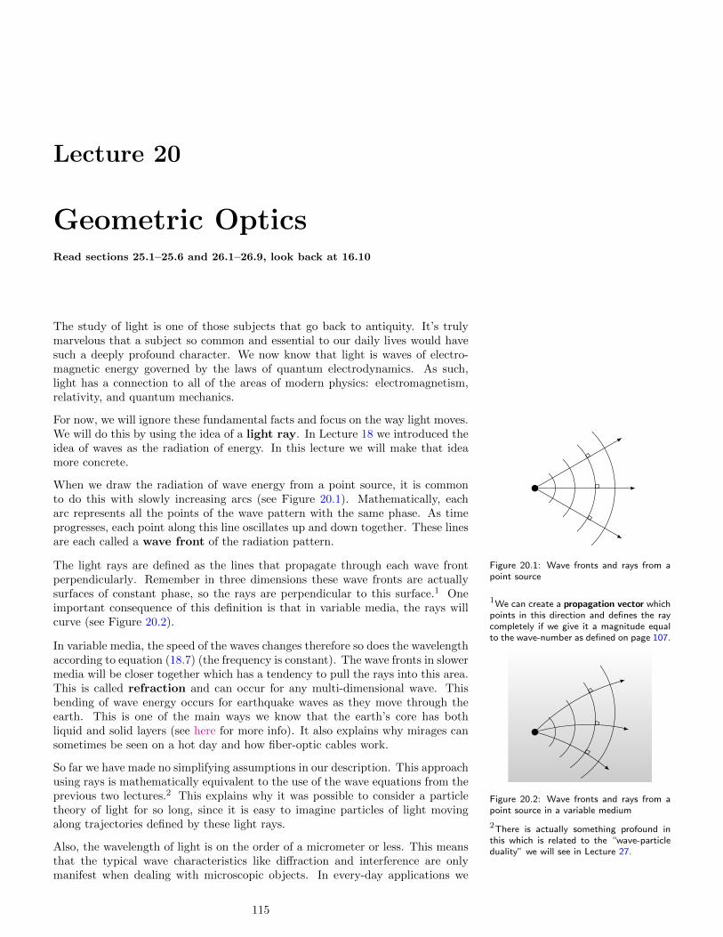
Lecture 20

Geometric OpticsRead sections 25.1–25.6 and 26.1–26.9, look back at 16.10

The study of light is one of those subjects that go back to antiquity. It’s trulymarvelous that a subject so common and essential to our daily lives would havesuch a deeply profound character. We now know that light is waves of electro-magnetic energy governed by the laws of quantum electrodynamics. As such,light has a connection to all of the areas of modern physics: electromagnetism,relativity, and quantum mechanics.

For now, we will ignore these fundamental facts and focus on the way light moves.We will do this by using the idea of a light ray. In Lecture 18 we introduced theidea of waves as the radiation of energy. In this lecture we will make that ideamore concrete.

When we draw the radiation of wave energy from a point source, it is commonto do this with slowly increasing arcs (see Figure 20.1). Mathematically, eacharc represents all the points of the wave pattern with the same phase. As timeprogresses, each point along this line oscillates up and down together. These linesare each called a wave front of the radiation pattern.

Figure 20.1: Wave fronts and rays from apoint source

The light rays are defined as the lines that propagate through each wave frontperpendicularly. Remember in three dimensions these wave fronts are actuallysurfaces of constant phase, so the rays are perpendicular to this surface.1 One

1We can create a propagation vector whichpoints in this direction and defines the raycompletely if we give it a magnitude equalto the wave-number as defined on page 107.

important consequence of this definition is that in variable media, the rays willcurve (see Figure 20.2).

Figure 20.2: Wave fronts and rays from apoint source in a variable medium

In variable media, the speed of the waves changes therefore so does the wavelengthaccording to equation (18.7) (the frequency is constant). The wave fronts in slowermedia will be closer together which has a tendency to pull the rays into this area.This is called refraction and can occur for any multi-dimensional wave. Thisbending of wave energy occurs for earthquake waves as they move through theearth. This is one of the main ways we know that the earth’s core has bothliquid and solid layers (see here for more info). It also explains why mirages cansometimes be seen on a hot day and how fiber-optic cables work.

So far we have made no simplifying assumptions in our description. This approachusing rays is mathematically equivalent to the use of the wave equations from theprevious two lectures.2 This explains why it was possible to consider a particle

2There is actually something profound inthis which is related to the “wave-particleduality” we will see in Lecture 27.

theory of light for so long, since it is easy to imagine particles of light movingalong trajectories defined by these light rays.

Also, the wavelength of light is on the order of a micrometer or less. This meansthat the typical wave characteristics like diffraction and interference are onlymanifest when dealing with microscopic objects. In every-day applications we

115

can ignore the wave nature of light and assume that light rays obey the laws ofgeometric optics:

• Rectilinear propagation. In a uniform transparent medium without obsta-cles, light rays move in straight lines. (This is why shadows are sharp).

• Law of reflection. When encountering a reflective surface, light rays willbounce so that the angle of reflection equals the angle of incidence.

• Law of refraction. When encountering a change in transparent media, therefraction angle of the ray is governed by Snell’s law (20.4).

We will discuss refraction shortly—for now we focus our discussion of reflection.In and of itself, reflection is pretty easy to understand: it’s not unlike a ballbouncing off of a wall. Where things start to get interesting is when we use thisreflection to focus light with the use of a lens.

Circular lenses are not the optimal cross-section for a lens, but circular lenses aremuch easier to make and they work reasonably well if the size is not too large.3

3The best cross-section is a parabola whichis why high precision instruments like radiotelescopes are this shape. The headlightson your car are this shape too.

This is called the “thin lens approximation”.

If we take a small circular mirrored lens, it will focus incoming rays of light ata point halfway between the center of the circle and the far edge of the lens(see Figure 20.3). This is because the angle of reflection is measured off of theperpendicular from the mirror which goes through the center. This is called thefocal point of the lens.

fC

Figure 20.3: Focal point of a circular mir-rored lens

The defining characteristic of the focal point is that parallel rays will meet at thefocal point after being reflected off the mirror. We can use this fact to determinethe location of the image reflected from the mirror.

Figure 20.4: The image of an object outsidethe focal length is inverted and real

Consider Figure 20.4. The object is on the left and we consider two very particularlight rays which leave the tip of the arrow. The first ray runs horizontal and weknow that this ray will bounce through the focal point and continue on down. Thesecond ray goes directly to and through the focal point. We know that this raywill bounce and then run horizontal because the geometry is the same whetherthe rays run backward or forward. These two lines intersect at the location of theimage. If we were to put a screen here, we would get a sharp image of the object.The rays of light appear to be generated from this spot and it is therefore calleda real image.

After examining the geometry of this situation (the upper and lower triangles aresimilar), the lens equation that governs this is

1

do+

1

di=

1

f(20.1)

where do is the distance from the object to the lens and di is the distance fromthe image to the lens. The magnification of the height of the image is

m = − dido

(20.2)

The negative sign indicates the image is inverted.

Though equation (20.1) is the commonly used lens equation, it can also be shownthat

xoxi = f2 (20.3)

where xo and xi are the distances from the focal point to the object and image,respectively. This form of the lens equation is due to Newton (the other isassociated with Gauss) and to my mind a bit easier to derive from the ray diagramin Figure 20.4.

116

After playing with these equations for a while, you may notice that equation(20.1) gives a negative image distance if the object is within the focal length ofthe mirror (i.e., do < f). This is still correct and is telling us that the image islocated on the other side of the mirror (see Figure 20.5).

Figure 20.5: The image of an object insidethe focal length is upright and virtual

In this case the image is said to be a virtual image because although thelight rays appear to be coming from this point in space, they never do go there.Putting a screen behind the mirror will not capture a sharp image of the objectno matter how hard you try. Notice that the magnification equation (20.2) stillworks because the negative image distance yields a positive magnification whichimplies the image is upright.

So far we have only discussed lenses that are convex. All the same principles applyfor a mirror that is concave in shape (see Figure 20.6). For a concave mirror, thefocal length is negative since parallel lines will diverge giving the impression thatthe image is behind the mirror. In fact, the image in a concave mirror is alwaysvirtual.

ConvexConcave

Figure 20.6: Lenses concave and convexWe can continue and talk about combinations of mirrored lenses, but the math-ematics always involves using equations (20.1) and (20.2). The important pointto remember is that the image of the first lens becomes the object of the next. Inthis way we can daisy-chain our way through any combination of lenses.

We are now ready to discuss the third law of geometric optics: refraction. Thoughthe ancient Greeks knew about the law of reflection, they never could quite getthe law of refraction. The correct law (known as Snell’s law) was discovered inthe early 1600s:

n1 sin θ1 = n2 sin θ2 (20.4)

This governs the angles involved when a light ray encounters a sharp boundaryin the transparent medium. The values of n1 and n2 are called the index ofrefraction for the material and the angles θ1 and θ2 are measured from thenormal line to the surface (see Figure 20.7).

θ1

θ2

n1 = 1.00

n2 = 1.58

Figure 20.7: Snell’s law of refractionThe index of refraction is a measure of the “refractive power” of the material.The higher the value of n, the more light will bend when entering it from the air.Though values can vary based on the composition of the material, typical valuesare listed in Table 20.1. By definition, the index of refraction of vacuum is one.

Air 1.0

Water 1.3

Glass 1.5

Diamond 2.4

Table 20.1: Typical indexes of refraction

If we shine a ray of light from inside a larger index of refraction material to asmaller one, the ray will bend outward according to Snell’s law (20.4). Thereis a particular angle (called the critical angle) in which the refracted ray iseffectively at 90 to the surface. Any incident angle beyond this is said to suffertotal internal reflection because none of the light energy is transmitted out. Themeasurement of the critical angle for a substance is an easy way to accuratelydetermine its index of refraction.

As we noted at the beginning of this lecture, the refraction of a wave is relatedto the propagation speed of the medium. This is true of the index of refractionas well. The relationship is simple:

n = c/v (20.5)

where c is the speed of light in vacuum and v is the speed of light in the material.

Of course we can use the refractive power of a material to create a lens too. In justthe same way as with a reflective lens we define the focal point to be the locationwhere parallel lines meet after passing through the lens. Interestingly because thisdefinition is the same as with mirrors, the geometry in the ray diagrams is verysimilar and the equations (20.1) and (20.2) also hold for thin transparent lensesalso. The one difference is that the sign conventions are different because imagesfrom a lens tend to be on the opposite side of the object. Table 20.2 outlines thedifferences.

117

Table 20.2: Sign conventions for use in the lens equations

This is positive when. . . Mirror Lens

Focal length (f) Convex Convex

Object distance (do) To the left To the left

Image distance (di) To the left To the right

Just as with multiple mirrored lenses, we can combine transparent lenses andanalyze the images using the lens equations. As before, the main principle is thatthe image of the first lens becomes the object of the next. Most microscopesand telescopes involve multiple lenses in order to magnify the objects underinvestigation.

One simple example is from optometry. The optical power of a lens is defined asthe reciprocal of its focal length (so stronger lenses have higher numbers). Thisrefractive power is measured in diopters which is simply one over one meter.When two lenses are touching, the refractive powers add.4. Since glasses and

4This follows directly from equation (20.1). contact lenses are typically quite close to the lens of the eye, this simplifies theanalysis of correcting vision by simply adding or subtracting diopters from thenatural power of the patient’s eye. The optical power of a normal eye is about 60diopters.

Isaac Newton was very interested in the study of light, performed many experi-ments, and wrote a major treatise on the subject. And it was he who discoveredthe principle behind the rainbow: that white light is actually all the colors of therainbow mixed. We can understand this realizing that most transparent materialsare dispersive (that is, the speed of wave propagation varies with frequency). Sincethe color of light corresponds to the frequency of the wave, we expect the indexof refraction to be color-dependent as well. Typically differences in color accountfor about a 2% change in the index of refraction.

We have already noted that circular lenses will only focus the light along arelatively small arc of the curve. If the arc is extended, the curve is too fastand pulls the rays in and away from the focus. This “de-focused” effect is calledthe aberration of the lens and is generally a thing to be avoided. The shapethat will focus all the parallel rays of light perfectly is a parabola and has noaberration due to its shape.

However, another way lenses are aberrant is due to dispersion. Aberration ofthis sort is called “chromatic”. It is sometimes possible to correct this kind ofaberration by combining lens of different indexes of refraction to bring all thecolors of light back together at the final focal point.

Other than equation (20.5), we have essentially ignored the speed of light. Nothingin the laws of geometric optics touches on the speed of light. Perhaps this is be-cause light speed is so fast. For all intents and purposes it travels instantaneously.Of course we now know this is not the case, but geometric optics is just that:geometric. There is no time component involved, no dynamics.

In the late 1600s, Pierre de Fermat discovered that all three geometric laws couldbe summarized in one simple principle: the principle of least time. The timerequired to travel from point A to point B is along any other path than the trueone takes more time. This was the first (and simplest) example of a variationalprinciple in physics and became an archetype for several others including theprinciple of least action which we mentioned in Lecture 7.

Next week will bring our study of waves and light to a close. We will discuss thewave nature of light—including diffraction and interference phenomena. Nearlyall of the concepts have been already introduced, but some interesting applicationswill be reviewed. We will mention how light is polarized. Also we will touch on

118

the distinction between coherent and incoherent light—which is the differencebetween laser light and ordinary light. Finally we will finish the discussion on aphilosophical note regarding the existence of the ether.

119

120

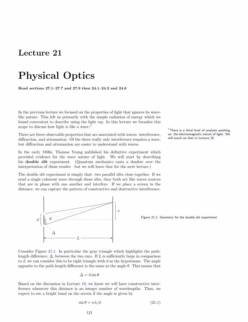
Lecture 21

Physical OpticsRead sections 27.1–27.7 and 27.9 then 24.1–24.2 and 24.6

In the previous lecture we focused on the properties of light that ignores its wave-like nature. This left us primarily with the simple radiation of energy which wefound convenient to describe using the light ray. In this lecture we broaden thisscope to discuss how light is like a wave.1

1There is a third level of analysis awaitingus: the electromagnetic nature of light. Wewill touch on that in Lecture 26.

There are three observable properties that are associated with waves: interference,diffraction, and attenuation. Of the three really only interference requires a wave,but diffraction and attenuation are easier to understand with waves.

In the early 1800s, Thomas Young published his definitive experiment whichprovided evidence for the wave nature of light. We will start by describinghis double slit experiment. (Quantum mechanics casts a shadow over theinterpretation of these results—but we will leave that for the next lecture.)

The double slit experiment is simply that: two parallel slits close together. If wesend a single coherent wave through these slits, they both act like waves sourcesthat are in phase with one another and interfere. If we place a screen in thedistance, we can capture the pattern of constructive and destructive interference.

L

θd

x

∆

Figure 21.1: Geometry for the double slit experiment

Consider Figure 21.1. In particular the gray triangle which highlights the path-length difference, ∆, between the two rays. If L is sufficiently large in comparisonto d, we can consider this to be right triangle with d as the hypotenuse. The angleopposite to the path-length difference is the same as the angle θ. This means that

∆ = d sin θ

Based on the discussion in Lecture 19, we know we will have constructive inter-ference whenever this distance is an integer number of wavelengths. Thus, weexpect to see a bright band on the screen if the angle is given by

sin θ = nλ/d (21.1)

121

Of course, this same angle is given by tan θ = x/L. So we can reverse equation(21.1) to determine the wavelength of this light by measuring the distance x.

The main obstacle to overcome when observing the interference of light is thesmall wavelength. The range for the human eye is about 390 to 750 nanometersfor blue and red light respectively. The interference pattern depends on thiswavelength so it is typically very hard to see unless the geometry is of the sameorder. Also the wavelength dependence means that the pattern is best seen formonochromatic (single color) light.

The double slit experiment requires that light wave as the two slits be in phase.This is why firing two lasers at a screen will not produce interference. The wayYoung accomplished this was by placing a preparatory screen in front of thedouble slit. In this screen was a single slit essentially acting as a wave source forthe double slit.

Another way to accomplish this is by taking splitting a coherent beam of light.This is usually done with a half-silvered mirror which reflects half the beam andtransmits the other half. The arrangement in Figure 21.2 is called the Michelsoninterferometer is able to measure the speed of light with great accuracy. Essen-tially the interferometer is able to measure the distances between the two mirrorswithin 0.1 microns (the wavelength of light). Michelson and Morley originallydesigned this apparatus to detect the “ether wind” (a topic to which we willreturn in Lecture 26).

Figure 21.2: Schematic of the Michelson interferometer

Half silvered mirror

Source

Mirror

Mir

ror

Young’s original double slit experiment depends upon the diffraction of light.This is the tendency for waves to bend around obstacles and why you can heararound corners. This is why the light bends and interferes in his double slitexperiment rather than simply casting a very sharp shadow of the two slits.

If we were to remove a slit from Young’s arrangement, the remaining slit will castits shadow on the screen. But since the slit is small, the shadow will be fuzzy duethe diffraction. In fact, the intensity of the diffraction pattern is given by2

2The function sin(x)/x is called the sincfunction and happens to be the Bessel func-tion shown in Figure 18.3. The connectionhere is merely coincidental as far as I know.

I =

[(λ

πaθ

)sin

(πaθ

λ

)]2

(21.2)

where a is the width of the slit (see Figure 21.3). This function assumes that thedistance to the screen is much larger than the slit width so that the rays of lightare effectively parallel from the slit.3

3Technically, L a2/λ. This approxima-tion is called Fraunhofer diffraction. Forscreens very close Frensel diffraction cor-rects the calculation.

The diffraction given by equation (21.2) drops to zero whenever

θ = nλ/a (21.3)

except when n = 0 which is the brightest point of all. So even with a single slitwe can see the wave nature of light. However, the side lobes of equation (21.2)are usually very faint, so effectively the image is spread over the range defined by(21.3) with n = 1.

122

λ aθ Figure 21.3: Single slit diffraction pattern (slit width exagger-

ated for clarity)

The previous analysis was all performed assuming the diffraction aperture wasa thin slit. Another common type of aperture is a small circular hole. Thediffraction pattern in this case is radial, but has the same characteristics asequation (21.2) except the pattern is slightly wider.4 The width of the central

4This radial pattern is called the Airy disk.Calculating the diffraction pattern from anyaperture involves Fourier transforms whichare closely related to the Fourier analysis wementioned in Lecture 19.

diffraction peak is given byθ = 1.22λ/a (21.4)

where a in this case is the diameter of the circular aperture.

Since the typical aperture in a telescope is circular, we expect the images of stars toexhibit just this kind of diffraction. An important consideration is the resolutionof the images from two stars. We can use equation (21.4) as an objective measureof resolution. We say that we can distinguish two sources if the diffraction peaksdo not overlap. This is called the Rayleigh criterion (see Figure 21.4). In fact,when using the human eye, the pupil is the effective aperture. Using equation(21.4) and 570 nanometers as the average wavelength of light, we can say that thehuman eye can resolve images with an angular separation of 1.4× 10−5 radians,or about 100 arc-seconds.

Figure 21.4: Point sources are resolved ifthe central diffraction peaks do not overlap

A diffraction grating is effectively a double slit analysis on steroids. A diffrac-tion grating is good at displaying the wave nature of light because it separatesthe colors through interference rather than dispersion. Consider for a momentthe geometry of the triple slit in Figure 21.5.

L

2d

x

Figure 21.5: Geometry for a triple slit

The path-length difference emphasized by the gray triangle still governs theinterference pattern. The lower slit introduces a third ray with an extra ∆ of path-length difference. What this means is that when the double-slit angle producedconstructive interference, the triple-slit also does. However, when the top two slitsare in destructive interference, the third will propagate through. The diffractionpattern still peaks at the constructive interference points given by equation (21.1),but the peaks are much shaper (narrower and taller).

A typical diffraction grating will have much more than three slits. Typically weare told the number of slits per centimeter or some similar metric. The angle ofdiffraction is proportional to this number.

A diffraction grating will disperse light into a rainbow because equation (21.1)is wavelength dependent. A standard DVD produces this effect because of theclosely spaced tracks on the disk. The regular spacing in crystals will also act like

123

a diffraction grating for certain wavelengths of light. This kind of analysis is howthe double helix structure of DNA was first discovered.

Usually the iridescence seen in nature is not from a diffraction grating, however. Itis much more common for this effect to be produced by thin-film interference.Simple examples include soap bubbles and the colorful sheen of oil on water.

Physically this occurs because both the inner and outer boundary act as reflectionpoints. The light from the front of the layer will constructively interfere with thelight from the back of the layer if the distances are just right (see Figure 21.6).

λ1

t

n1

n2

Figure 21.6: Thin film interference If the thickness of the film is t, the path-length difference is 2t, so you might thinkwe require 2t = mλ (we use m to avoid confusion with the index of refraction).However, the reflection from the front is a hard reflection because the refractiveindex of the film is larger than air. The reflection off the back is a soft reflectionfor similar reasons, so the interference acts something like the open tube fromLecture 19. This means we require

2t = (m+ 12 )λ2

where λ2 is the wavelength of the light in the medium. But we know that thewavelength of the light changes with any change in the index of refraction becauseits speed will change. We combine equations (20.5) and (18.7) with the previouscondition to yield the thin-film interference formula:

2t = (m+ 12 )

(n1

n2

)λ1 (21.5)

where we give the wavelength the subscript 1 to emphasize that this is the sourcewavelength.

You might wonder why the film must be thin. The reason is that the two rays mustbe of comparable amplitude in order to interfere. Typically as light moves througha transparent medium, it loses intensity. This is called attenuation and is a kindof optical friction or resistance. It is possible to incorporate this attenuation byallowing the index of refraction to be a complex number, though we will not doso here. The attenuation of light causes the intensity to fall exponentially.

There is another characteristic of light that is a consequence of its wave nature:coherence. This is the difference between incandescent light and laser light.In laser light, each pulse of light is aligned by both phase and polarization.5

5This occurs because a type of standingwave is built in the lasing material whichexcites more coherent light via a quantummechanical process. Although the produc-tion is based on quantum mechanics, thecoherence of the light is understandablewith classical ideas.

This means that effectively all the light rays constructively interfere all the time.With an incandescent light, the alignment of phase and polarization is random:sometimes its constructive, sometimes its destructive.

Since the intensity of the light is proportional to the square of the amplitude,when the intensity of the incandescent bulb increases two-fold, the intensity oflaser light increases four-fold. So, the high intensity of laser light is due to thecoherence of its light—which is a wave phenomena.

Another piece of evidence for the wave nature of light is its polarization. Thepolarization of light was first discovered through birefringence: a material inwhich the index of refraction depends upon the polarization of the light. A typicalimage seen through this material will double as the light is polarized relative toits crystal structure.

The best way to explain why the polarization of light cannot be explained byparticles is by considering two crossed polarizing filters. When we pass lightthrough a filter, the component of the light wave aligned with the polarizer axispasses through. If we place a second polarizer at 90 to the original, it will blockthe light because there is no component left to pass through.

If, however, we insert a third polarizer in between them aligned at an angle, lightwill begin to pass through again. When two polarizers are at an angle θ, the

124

intensity of light that passes through is given by Malus’ law:

I = I0 sin2 θ (21.6)

This is because the intensity is proportional to the square of the amplitude andthe polarizer allows a component A = A0 sin θ through.

If the middle polarizer is set at 45 then it will let half of the intensity of lightthrough. The final polarizer is also at 45 to the middle, so one-quarter of theintensity of light is allowed through even though the two outer polarizers arecrossed.

So, the evidence is pretty clear that light is a wave phenomena. Of course everywave does so in a medium and it is natural to ask what is the medium for lightwaves? In the 19th century this medium was given the name the ether and oneof the main goals was to determine its mechanical properties.

But what is it? Like an elastic solid transmitting sound waves? This substancemust be present everywhere light is—including the depths of outer space. Ap-parently it is everywhere, yet we do not experience any “ether drag” like we dowith air. If we model this as an elastic solid, its wave speed is given by equation(18.2). But the speed of light is enormous. This implies a very rigid solid whichis less dense than air—yet its presence is undetectable mechanically. The searchfor an “ether wind” was a hot topic around the turn of the 20th century.

As the evidence piled up, it began to be more and more difficult to imagine anymechanical model that could act as a medium for light. During this time, Ein-stein’s special theory of relativity altered our views of space and time effectivelydeclaring the ether concept dead. Now, with the advent of quantum field theory,we no longer even think of light as waves—but that’s the subject for next week.

Next week we will continue discussing mechanical models for the ether. We willfind that the more we refine this model, the more problems we uncover. This isone of three major breeches in classical mechanics. In this case, the problem isfinally resolved in the theory of relativity. On the other hand, we have quantummechanics as the resolution of the other two problems (kinetic theory and atomictheory). In this way we will finish the term recognizing the limits of classicalmechanics.

125

126

Lecture 22

Limits of ClassicalMechanicsReview Lectures 16 and 21. Sneak a peak at sections 28.6–28.7, 29.1–29.3and 30.3

In the last lecture we left open the question on the ultimate nature of light. Theevidence for some sort of wave picture is clear. However, the mechanical nature ofthe medium doing the waving was less clear. By the middle of the 19th century,some connection between electricity, magnetism, and light was understood. Aselectromagnetic theory matured (culminating in Maxwell’s equations), the prob-lem became worse.

One clear example is that light (as an electromagnetic wave) should carry mo-mentum. The problem is that mechanical waves do not carry momentum. Thetransfer of momentum implies a transfer of mass: movement of the medium itself.

Well, perhaps the ether is a fluid. A fluid can easily carry momentum and supportwave motion. In fact, a thought at the time held that elementary particles mightbe modeled as a vortexes in the fluid. Like a smoke ring, a vortex can maintainits structure over an extended period of time.

Unfortunately, a fluid cannot support a polarized wave. Because a fluid only haspressure stress (no shear or normal stress), the compression wave has only onedegree of freedom. But electromagnetic theory and experimental results requirea polarized wave theory of light.

Whether solid or fluid, we expect a basic result called the “ether wind”. Whenyou are riding a car and roll down the window, can you tell you are moving? Ofcourse you can: the wind gives it away. The air is not moving: the wind is causedby your motion through the medium. In the same way, we ought to be able todetect our motion through the ether.

Of course, our motion needs to be comparable to the speed of light—which isfast. One trick was to measure this ether wind by using the motion of the earth.Around the turn of the 20th century, Michelson and Morley performed a numberof experiments to detect the motion of the earth through the light ether. Thenow famous “null result” caused quite a bit of controversy at the time. Theoryafter theory was proposed1 but the whole thing reminds one of the epicycles of

1For example, maybe the earth moves insome sort of ether bubble.

Ptolemaic astronomy. Tweak after tweak attempting to fit a dying theory tounyielding facts.

The answer was summarized in 1905 by Einstein in the special theory of relativity.By the statement that E = mc2, we can see that every wave moves mass throughthe energy it moves. For everything except a light wave, the amount of mass is

127

completely negligible. But for light, the momentum transfered follows from thisformula.

However any mechanical model of light based on Newton’s laws was in contra-diction with the principle of relativity (see page 27). Because this medium isuniversal and everywhere, it acts as an absolute reference frame. But Einsteinshowed that it is possible to have our cake (electromagnetic theory) and eat ittoo (principle of relativity) and declared the ether dead.

The trade-off is that we must reassess our assumptions about space and time.Because of this the speed of light acts as a universal speed limit which impliesthat speed and velocity works in a way that is non-Newtonian. This explains thenull result of Michelson and Morley, but at the expense of bizarre consequenceslike length contraction and time dilation. We will return to these ideas in Lecture26.

Relativistic mechanics wasn’t the only correction required to classical mechanics.In many ways quantum mechanics was an even more radical correction thanrelativity. Interestingly, Einstein played a large role in development of quantummechanics too.

Looking back now, the first hint how wrong we were to assume the subatomicworld operated under classical principles of mechanics was the ultraviolet catas-trophe. This comes from the analysis of the spectrum of radiation from a heatedobject. The net power radiated is given by equation (15.3), but what we seekis the distribution of this energy across the electromagnetic spectrum. Classicaltheory predicts an ever-increasing amount of energy in the lowest wavelengths,which is nonsense.

In 1893, a result known as Wien’s Law was empirically discovered:

λmax =2.898× 10−3

T(22.1)

In this formula, the peak wavelength in the spectrum is inversely proportionalto the absolute temperature. Ultimately, quantum theory predicts a spectrum inline with reality (see Figure 22.1) and justifies Wien’s law.

λ

dE

Classical

QuantumQuantum

Visible

Figure 22.1: Ultraviolet catastrophe: Ex-pected spectrum of energy by wavelengthfrom a hot object. Both curves assume atemperature of 5000 kelvin—the approxi-mate temperature of the sun.

In both classical and quantum theory, the number of ways a medium can vibrate(i.e., its modes, see page 112) is proportional to the square of the frequency.2 If the

2This assumes the medium is three di-mensional. For a string (one-dimensional),the number of modes is constant acrossfrequency. For a sheet, the number ofmodes increases linearly with frequency.

medium is in thermal equilibrium at a particular temperature, the equipartitionprinciple from kinetic theory (page 96) implies that each mode will hold kT unitsof energy.

If the ether is a classical wave medium, this implies that the amount of radiantenergy from a hot object should be dominated by the high frequency, low wave-length (ultraviolet) range of the electromagnetic spectrum—in other words, hotobjects should be blue rather than red. Classic theory is not even close. Relativitydoesn’t save us here because the energies involved are no where near relativistic.

In 1900, Max Planck was able to mathematically reverse engineer the actual radia-tion spectrum and came to the conclusion that the problem was the equipartitionprinciple. He found that with a single simple assumption, he could derive thecorrect spectrum:

∆E = hf (22.2)

In other words, the modes are only allowed to exchange energy in increments thatare proportional to the frequency of that mode. This has the effect of suppressingthe higher frequency modes because the probability of a large energy exchange isexponentially small in thermal equilibrium.

Another phenomenon points to an unusual connection between energy and fre-quency3 of light called the photoelectric effect first discovered in 1839. If one

3Remember: classically, energy in a wave isrelated to its amplitude not its frequency.

shines intense light on metal it will ionize and the electrons thus stripped off can

128

be captured in an electric current and measured. The odd thing is that the speedof the escaping electrons depends on the frequency of the light. In fact, for verylow frequency light no electrons are released no matter how intense the light.

But why? A few years later, Einstein realized that both Planck’s assumptionand the photoelectric effect can be explained through a particle theory of light.Each particle, called a photon, has energy related to its frequency according to(22.2). It is actually this work rather than relativity for which Einstein receivedhis Nobel Prize in 1921.

Einstein realized that the explanation of the photoelectric effect is simple if lightcomes in streams of photons. Each photon only carries hf worth of energy, so ifthe frequency is not high enough, the light particle does not have enough energy tolift the electrons out of the potential well that binds them in the atom. Increasingthe intensity of light only increases the number of photons—none of which arepowerful enough to move the electrons.

The most important thing about the photoelectric effect is that it cannot beexplained with waves. This frequency dependence of energy is without parallelin the classical theory. The fact that energy transfer is quantized by (22.2) isunprecedented.

And there were other problems—particularly at low temperatures. The specificheat of solids predicted by classical theory was wrong (Einstein also proposed thefirst approximation of a solution using quantum ideas). Superconductivity wasdiscovered in which the electrical resistance of a metal disappears. Liquid heliumbelow about 2.17 degrees kelvin completely loses all viscosity (now known as asuperfluid).

Beside issues with classical kinetic theory, deep inconsistencies were discoveredin the structure of the atom. Classical electromagnetic theory implies that anorbiting electron will continually radiate energy. Based on the size of the atom,the theory predicts that all the orbital energy should be radiated away in 10−11

seconds or so. Atoms are a bit longer lived than that: another blatant contradic-tion between theory and reality.

Spectroscopy is the study of the spectrum of radiation from materials. It wasdiscovered that the elements only emit radiation along certain frequencies: cre-ating a pattern of lines rather than a smooth spectrum. Both this and the non-radiating orbital electron seem to imply that energy transfer is limited in themicroscopic realm. The Bohr model of the atom (see Lecture 28) was successfulin collecting these facts, but left unexplained the fundamental reason of whyenergy is quantized.

Out of this cacophony of confusion quantum mechanics was born. Nearly 30years of struggle and debate finally gelled into a single explanation—which isthe subject of Lecture 27. Einstein’s photon idea combining particle and wave(in some obscure way) led Louis de Broglie to postulate that perhaps elementaryparticles (in particular: electrons) have both particle and wave characteristics too.These “matter waves” are critical in understanding the structure of the atom andform the foundation of chemistry.

So around 1925 order was brought back to the land of physics. Except one thing.Quantum mechanics is not relativistic. And the most straightforward way tocombine the two was fraught with problems (like negative kinetic energy, infinitenumbers of particles, etc.). It took another quarter of a century to realize thatthe conflict between quantum mechanics and special relativity was only on thesurface. The development of quantum electrodynamics (QED) has been describedas the “crown jewel of physics” by Feynman due to its astonishing accuracy (betterthan ten parts per billion so far).

The mathematical framework for QED is called quantum field theory (see Lecture

129

27). One important consequence of quantum field theory is the division of theworld of elementary particles into fermions and bosons. The electron is anexample of a fermion which ultimately explains the periodic table. The photonis an example of a boson which ultimately explains Planck’s solution to theultraviolet catastrophe. Fermions are the building blocks of matter and bosonsare the carriers of force.

Quantum field theory has been utilized to explain the two nuclear forces as well.Though more complicated, these theories are also accurate to within currentexperimental precision. So the fundamental framework of subatomic physics isable to explain every experiment to date. This is called the Standard Model ofphysics (see Lecture 30).

But the holy grail, the “theory of everything”, still eludes us. Oddly enough, it isgravity—the first force of them all—that stands alone. It took Einstein a dozenyears to discover a relativistic theory of gravity (general relativity). No one hasdiscovered a quantum theory of gravity. Stay tuned.

130

Lecture 23

The Electric Field andPotentialRead sections 18.1–18.9 and 19.1–19.5

Electricity, magnetism, and gravity are all long-range forces. Rather than actingvia the direct contact of objects (like elasticity or friction), these forces act “ata distance”. Though gravity was the first to be quantified in Newton’s inversesquare law (6.3), magnetism was the first to be studied. Perhaps due to itsportability: one can play with magnets much easier than planets.

In 1783, it was discovered that the electric force also obeys the inverse squarelaw1

1All three long-range forces roughly obey aninverse square law. Interestingly, only theelectric force obeys the inverse square lawexactly.

F =kqQ

r2(23.1)

which is called Coulomb’s law. Each q represents the electric charge on theobject and k has a value of 8.9876× 109 in SI units.2

2We will see why in Lecture 26, but thishappens to be the speed of light squaredtimes 10−7.

Unlike gravity (and like magnetism), the electric force is both attractive andrepulsive. This implies that there are two different kinds of electric charge. Theconvention to call them “positive” and “negative” goes back to Benjamin Franklin.One advantage to this convention is that equation (23.1) now tells us when theelectric force is attractive (charges of the same charge) or repulsive (charges ofopposite charge).

It is not hyperbole to say that our modern standard of living depends on thecorrect understanding and harnessing of electric power. In general, materials fallinto two categories: conductors which easily allow the flow of electric chargeand insulators which essentially block the flow.3

3These terms are used in the context ofanything that flows: for example, heat.Take an object with some excess charge on it. If we touch this object with a

conductor, some of the excess charge will flow into and through the conductorbecause all of the individual charges are repelled from one another. In general,any excess charge will distribute itself through a conductor in order to maximizethe distance between the charges. This is also why any excess charge will resideon the surface of a conductor.

There is another, trickier, way to transport electric charge. Take the same objectas before with the same excess charge on it. Move the conductor close to theobject without touching it (or place a thin insulator between them). The chargein the object will repel similar charge in the conductor and attract the oppositecharge. In this way, a separation of charge is induced in the conductor. If wedrain the repelled charge (by connecting it to the ground—literally), we are leftwith a net charge in the conductor of the opposite polarity.

131

These tricks were essential to the initial study of electricity. They also reveal animportant fact of nature: matter is electrically active. Of the three long-rangeforces, electricity is the most powerful. Ironically, this strength acts to concealthe electrical nature of matter. Negative electrons4 are strongly attracted to the

4There are about 6.25 trillion electrons in acoulomb, the SI unit of electric charge.

positive nucleus and lock into an overall neutral atom. Except for unusual (anddramatic) circumstances, electricity is only manifest on the microscopic scale.

But, indirectly, electricity is everywhere because it is the source of all elastic, con-tact, and chemical forces. In fact, every macroscopic interaction except gravity isultimately electric. In most cases, we need quantum mechanics to fully understandhow this is true (in particular, the solidity of matter and the covalent bond). Thekey insight is to recognize that any asymmetry in charge distribution can inducea similar asymmetry in adjacent atoms. This charge separation is idealized inthe dipole moment which is the product of magnitude of the charges and theseparation between them (see Figure 23.1).

+q

−q

p = qd

Figure 23.1: Dipole moment calculation In the mid-19th century, Micheal Faraday introduced the idea of the electric fieldinto the physics community. He found it necessary to conceptualize what washappening in certain electromagnetic experiments (we will see these in Lecture25). A couple of decades later, Maxwell summarized the dynamics of the electro-magnetic field in his four famous laws. Forty years later, Einstein realized thatthese laws are not compatible with Newton’s laws of motion and developed thespecial theory of relativity. He later emphasized that the field concept was thekey to uncovering the incorrect assumptions underneath Newton’s laws of motion.

The field also occupies a middle ground for those uncomfortable with “action-at-a-distance” by offering an intermediate entity to carry the influence of the force.We take Coulomb’s law (23.1) and divide it into two pieces

F = (q)

[kQ

r2

]which isolates (in square brackets) the part that is not associated with the chargeexperiencing the force. We call this the electric field generated by the chargeQ. In short, the electric field from a point charge is

E =kQ

r2(23.2)

and we can rewrite equation (23.1) as F = qE which makes clear why the SI unitfor the electric field is newtons per coulomb. The field from multiple charges issimply the sum of the fields from each. Though recognize that the field is a vector(because force is) so some vector addition may be required.

+q

Figure 23.2: The electric field around apoint charge represented by lines of flux

We can draw the electric field around a charge as in Figure 23.2. Each linerepresents electric flux which points in the direction of the force and the fieldstrength is represented by the density of flux lines in the diagram. Lines of fluxalways point from positive charges and end with negative charges (or drift off toinfinity).

The superposition of multiple charges can easily create quite complicated fieldline patterns. The simplest is produced by an infinite sheet of charge. Assumingthe charge density is constant (which it should be if the charges are at rest),then by symmetry we can see that the field lines will simply be straight linesperpendicular to the sheet. Since the field lines don’t diverge, this represents aconstant electric field.

If we place a dipole in the presence of a constant electric field, the positive chargewill be pulled along the field and the negative charge will be pulled against thefield. In Lecture 10 we called this a force couple and the effect is to produce anet torque on the dipole. The total torque acting on the dipole is given by

τ = pE sin θ (23.3)

132

where θ is the angle between the dipole moment and the electric field. So thedipole will twist until it lines up with the field.

Suppose we place a second sheet of opposite charge parallel to the first. Thiscreates a capacitor (see Figure 23.3). A capacitor is said to store charge sincethe charges on the two plates are held in place by their mutual attraction to oneanother. For a perfect (infinitely long) capacitor, there is no electric field on theoutside. True capacitors always have edge effects, so not all the electric fieldis contained inside the system. Also, the two plates of a capacitor are typicallyseparated by an insulator which allows a small amount of charge to flow andwill eventually neutralize the charge separation. This is called leakage in thecapacitor. + −

+ −

+ −

+ −

+ −

E

Figure 23.3: The electric field inside an idealcapacitor is constant

From Lecture 18 we know that the power intensity (18.8) from a point source fallsoff according to an inverse square law. The total energy is conserved but as theradiation propagates through space it is spread across a larger and larger surfacearea according to 4πr2. The mathematics is similar for the electric field from apoint charge. This means that for the electric field, the total flux is conserved.This is summarized in Gauss’ law:∑

surf

Φele = Qtot/ε0 (23.4)

where Φele is the total electric flux that passes through the surface of interest andQtot is the net charge inside the surface. The symbol ε0 is called the electricconstant5 and is equal to 1/4πk which is 8.854× 10−12 in SI units. One way to

5I learned this under the name “permittivityof free space”, but the “electric constant”is much easier to remember!

interpret this equation is that every line of flux starts with a charge—no lines offlux start (or end) in thin air.

We need to be careful to account for only the component of the field line thatpasses perpendicularly through the surface, so the formula for the flux is

Φele = (E cos θ)(A) (23.5)

where θ is the angle between the field vector and the normal vector to the surfacearea A.

Gaussian surface

Figure 23.4: Applications of Gauss’ Law to the electric fieldaround a dipole (image credit here)

As an example of Gauss’ law in action, consider the dashed circle in Figure 23.4.Notice how each field line that goes out is compensated by a line that goes in.The net flow of flux is zero which corresponds to the total enclosed charge beingequal to zero.

+

+

+

+

+

A Φele = EA

Qtot = σA

Figure 23.5: Calculating the electric field in a capacitor withGauss’ law

A more substantial application of Gauss’ law is to calculate the magnitude of thefield in an ideal capacitor. According to Figure 23.5, the total charge6 enclosed

6Remember, all the charge is collected onthe surface of the conducting plate.

133

in a rectangular box parallel to the positive plate is σA, where σ represents thecharge density (i.e., σ = Q/A). The only flux contribution is from the face thatis parallel to the surface, so the total flux coming out of the box is EA. UsingGauss’ law (23.4) we can solve for the electric field as

E = σ/ε0 (23.6)

Mathematically, we say that Gauss’ law tells about the divergence of the field.Field lines are only created at positive charges (known as “sources”) and they areconsumed at negative charges (known as “sinks”). The field is also characterizedby its curl which tells how much the field twists and turns as we follow the flux(think about a whirlpool in water). The way we evaluate this curl is by followinga closed path and calculating the component of the field parallel to the path. Thetotal accumulation of field along this path is the amount of curl in the field. Theelectric field has no curl because it comes from a central force. In symbols wehave: ∑

loop

Et∆s = 0 (23.7)

where Et is the component of the field parallel to the little bit of loop ∆s we areat in the sum.

This should remind you of the discussion of conservative and non-conservativeforces in Lecture 7 (see page 40). The electric force is conservative and a potentialenergy function exists. So far, we have drawn an analogy between intensity andflux. There is also a correspondence to this potential energy: the field potential.Both stem from the connection between field and force in the equation F = qE.The field potential is defined7 as

7Unfortunately, the negative sign heremakes the signs in some calculationsconfusing—in particular the next equation(23.9). This sign convention propagatesthrough all of electromagnetism, so bewareof signs!

∆V = −Et∆s (23.8)

In other words, the electric potential V increases as we move against the fluxlines in the field. This is similar to pushing up a ball against the force of gravity.This formula also implies that the potential does not change as we move directlyacross the lines of force. The formula for the electric potential energy is simply8

8Compare this with the gravitational po-tential energy (7.3): mgh. Apparently thegravitational field is simply −g!

PEele = −qV (23.9)

The SI unit for electric potential is the volt. A common unit of energy at themicroscopic level is the “electron-volt” which is the charge of the electron (1.602×10−19 coulombs) times a volt. This is also why the electric potential is also calledvoltage.

An equipotential surface is the collection of all the points in the electric fieldwith the same value of potential or voltage. The previous paragraph impliesthat at each point the equipotential is perpendicular to the field lines. Theseequipotential surfaces are similar to the contour lines on a topographical mapand the way wave-fronts and rays are related (see Lecture 20).

When we place a conductor in the middle of an electric field, the surface of theconductor will form an equipotential. The reason is that any voltage differencecorresponds to a net electric force along the surface. But the charge in theconductor will flow until this pressure is equalized. This also implies that the fieldlines that touch a conductor will be perpendicular to the surface. The conductorpulls the field lines toward itself by redistributing its internal charge (see Figure23.6) until they are perpendicular.

Figure 23.6: Adding a conducting sphereto a constant electric field will cause thefield lines to bend into the conductor (imagecredit here)

The formula for the electric potential from a single point charge is

V =kQ

r(23.10)

134

From this formula, you can see that the equipotential surfaces around the chargeare spherical shells of increasing radius.

The advantage of using the field potential rather than the field directly is that itis not a vector. So the total potential is the simple sum of the potentials fromeach charge. For example, the potential from a dipole is

V =kq

r+− kq

r−(23.11)

where r+ and r− are the distances to the positive and negative charges respectively(see Figure 23.7).

r−r+

r

θ+q−q

d

Figure 23.7: Calculating the electric poten-tial of a dipole

If we are far from the dipole, these distances are nearly parallel and can beapproximated by9

9This is similar to the trick we used toanalyze the double slit in Lecture 21.

r± = r ± 12d cos θ

where r is the distance from the center of the dipole and d is the distance betweenthe charges. In addition, since r is much larger than d when we are far away, wecan use the binomial theorem (1.3) to say

1

r±=

1

r

[1±

12d cos θ

r

]−1

=1

r

[1∓

12d cos θ

r

]Putting this result into equation (23.11) gives us the far-field approximation forthe dipole potential:

V =kp

r2cos θ (23.12)

where p is the dipole moment equal to qd and shows that the potential drops withthe square of the distance from the dipole.

The simplest calculation of potential is inside a capacitor because the field isconstant. Using equations (23.8) and (23.6), the voltage difference across thecapacitor is simply

∆V = Qd/ε0A

Though an insulator can introduce leakage into the capacitor, it can also dramat-ically increase the ability of the capacitor to store charge. This is due to the factthat the charges on the capacitor plates induce dipole moments in the insulator(called the dielectric) which effectively reduces the distance between the positiveand negative charges. So with the same voltage difference, the capacitor will holda lot more charge. This relationship is called its capacitance:

C = Q/V (23.13)

For an ideal capacitor, we have

C = κε0A/d (23.14)

The symbol κ is called the dielectric constant and is the factor of increase dueto the dielectric between the capacitor plates.

Charging up a capacitor takes work. Each incremental charge that is added takesmore work because it is repelled by the ones that are already there. The workrequired for each must overcome the potential energy given by equation (23.9).But the voltage is constantly increasing. The total work required to bring acapacitor up to voltage is10

10The factor of one-half occurs here in thesame way it occurs in the formula for kineticenergy.

W = 12CV

2 (23.15)

Next week, we will cover two topics: electricity and magnetism. In the presentlecture we have only discussed what happens when charges are in equilibrium orat rest. In the following lecture we will discuss the flow of charge, or current.

135

This will allow us to investigate some simple electronic circuits with resistors andcapacitors.

In addition, we will introduce the magnetic force and discuss its basic properties.We will find a strong parallel between the electric force and the magnetic forcewith one significant exception: there is no such thing as a magnetic charge. Theapparent parallel will continue to erode as we discover that every flow of currentcreates a magnetic field. Ultimately, natural magnetism is nothing but the resultof electric charges in motion.

136

Lecture 24

Basic Electronics andMagnetismRead sections 20.1–20.8, 20.11–20.14 and 21.1–21.8

Every electric circuit is designed to control and harness the flow of electric charge.Electric current is defined as the amount of charge that flows through a particularsurface area each second:

I =∆q

∆t(24.1)

The SI unit for current flow is the ampere equal to one coulomb per second.Current is driven by a differential in electric potential or voltage. When a chargeis exposed to such a differential, it will accelerate according to Newton’s secondlaw (5.1). This is what happens in a cathode ray tube, for example. But normally,the flow of current in an electric circuit is controlled through resistance. Thismeans that current is flowing at some constant terminal velocity. And just toadd more confusion, this potential difference is typically called the “electromotiveforce” or EMF although it is technically not a force.

When current flows, energy is moving through the circuit. The power consumedby any electric circuit can be obtained by combining equations (23.9) and (24.1).We get:

P = IV (24.2)

An ideal battery is an electrical component which is able to maintain a constantvoltage difference across its terminals regardless of how much current flows. Allbatteries wear out, but good ones last, so we will assume that our batteries carry aconstant voltage differential. A battery provides direct current which is constantover time. We will consider a different form of current (alternating current) inLecture 25. V

+ −

Load

Ie−

Figure 24.1: A simple electric circuitEvery circuit has a source of voltage difference (a battery, a solar cell, an antenna).The rest of the circuit is called the “load” and is said to “drop” the voltage (seeFigure 24.1). Remember that a perfect conductor does not support a voltagedifference. So, in order for the circuit to be in a stable state, the voltage differentialfrom the battery must be absorbed in the rest of the circuit somewhere.

Notice that electrons are actually leaving the negative terminal of the battery andtraveling to the positive terminal. However, we will ignore this and consider thecurrent to flow from the positive to the negative terminal.1 Surprisingly, it rarely

1This is just a historical accident becausethe current carrier has a negative charge.When Franklin established the conventionin the 18th century, he guessed wrong.

makes a difference which way you imagine the current to flow.

The simplest electric circuit consists of a battery, a resistor, and two wires con-necting them. A resistor is specifically designed to drop the voltage and dispersethe energy through heat. The ratio of the amount of current that flows per volt

137

through a substance is called its conductivity, though it is much more commonto quote its reciprocal called resistivity which may depend on temperature. Anideal resistor has a constant resistance over all voltage ranges and therefore obeys

V = IR (24.3)

which is called Ohm’s law. The total resistance of a particular resistor will be acombination of its geometry and the natural resistivity of the material used. Wehave:

R = ρd/A (24.4)

where ρ is the resistivity of the material, d is the length of the resistor, and A isits cross-sectional area.V

+ −

R1 R2

Figure 24.2: A simple series circuit Now suppose we have two resistors connected to a battery as shown in Figure24.2. These are said to be in series because the current must from throughone before the other. Clearly, the current through each resistor is equal, and thevoltage drop is split between them. The total resistance is simply the sum of thetwo resistors:

R = R1 +R2 (24.5)

V

+ −

R1

R2

Figure 24.3: A simple parallel circuit

Another way to connect the two resistors is in parallel—see Figure 24.3. In thiscase, the current runs through the two resistors simultaneously. The current issplit and both resistors drop the total voltage. The net resistance of the twoparallel resistors is given by:

1

R=

1

R1+

1

R2(24.6)

Both equations (24.5) and (24.6) can be seen as consequences of equation (24.4).In the case of resistors in series we effectively increase the length of the resistor:since distance is in the numerator, the resistances add. But in the case of resistorsin parallel we effectively increase the area of the resistor and since the area is inthe denominator, the reciprocal of the resistances add. Equation (24.6) can alsobe rearranged as

R =R1R2

R1 +R2

We can add and combine resistors in many combinations. It is even possible tocombine them in ways which are neither in series or parallel. The flow of currentthrough any circuit is governed by two basic principles called Kirchoff’s laws:

• The current at any junction sums to zero. Be careful to take into accountthe direction of the current.

• The voltage around any loop sums to zero. Be careful to take into accountthe direction of the potential difference.

The first is based on the conservation of charge and the second on the conservationof energy—compare equation (23.7). For seriously complicated circuits it issometimes easier to set up the problem using these laws. But typically, we canwork the problem by considering the resistors in pairs, either series or parallel.V

+ −

R C

Figure 24.4: A simple RC circuit We can also add capacitors to our circuits. Consider Figure 24.4. Initially, currentflows through the resistor and charges up the capacitor. All the voltage dropsacross the resistor. But as the capacitor begins to charge up, it also begins todrop voltage according to equation (23.13). Since the voltage drop across theresistor is less, the total current flow is less by Ohm’s law (24.3). The flow ofcurrent exponentially decreases until the capacitor is essentially fully charged.The formula for the current is given by

I(t) = I0 exp(−t/RC) (24.7)

138

where I0 = V/R. The quantity RC is sometimes called the time constant forthe circuit. Typically the capacitor is considered fully charged after five timeconstants since the current flow is under 1% of its original level.

We are now ready for a complete change of subject. . . . Let’s talk magnetism. Theawareness of magnets and magnetism appears to go back thousands of years, butthe Chinese were the first to write about using magnetic compasses for navigationin the 11th century. The study of magnetism was also one of the few sciencesto advance in Europe during the Middle Ages culminating the work of WilliamGilbert (a contemporary of Galileo) in 1600.2

2In this work, Gilbert explained the workingof the compass needle by assuming theEarth to be a large magnet. He did notknow why the Earth is a large magnet, andneither do we.

After one has played with a set of bar magnets, it becomes clear that the ends ofthe magnet are special—we call them the poles of the magnet.3 We say that like

3The poles of a magnet are not actuallylocated at the ends of the magnet. Ratherthey are somewhat inside (about 1/6 fromthe end or so).

poles repel while unlike poles attract. There really is nothing to prevent us fromcalling one positive and the other negative, but for obvious historical reasons wecall these groups north poles and south poles.

Suppose we bring the north poles of two magnets together. They will repel whilethe south poles attract. This pair of forces will tend to twist the magnet. Inother words, each magnet experiences a net torque. This torque guarantees thattwo magnets will always be attracted to one another, even if they have to twistaround first.

Coulomb performed experimentation to quantify this magnetic force. The forcelaw is the same inverse square law that he found for electricity:

F =1

4πµ0

p1p2

r2(24.8)

where each p represents the strength of the poles and the constant µ0 is assignedthe value 4π × 10−7. This constant is called the magnetic constant.4 A pole

4Again, I learned this as the “permeabilityof free space”, but this is easier to remember

strength of one weber will repel a like pole placed at one meter with a force of107/(4π)2 newtons. The magnetic field and flux are defined in just the same wayas with the electric force.

But if one splits a magnet in two, one gets two magnets, not two poles. Thesmallest element of magnetism observed physically is not a magnetic pole but amagnetic dipole.5 In other words, there is no “magnetic charge”. This is why

5For this reason many authors avoid dis-cussing magnetic poles in detail.

there is no such thing as a magnetic conductor nor magnetic circuits. It alsoimplies that Gauss’ law for magnetic flux is simply∑

surf

Φmag = 0

Though an exact parallel between electricity and magnetism is broken, the twoare deeply interconnected. So much so that we are justified in considering themtwo aspects of a single electromagnetic force. The first step in this discovery isby recognizing that an electric charge can experience a magnetic force. This iscalled the Lorentz force:

F = qvB sin θ (24.9)

where v is the speed of the charge and θ is the angle between the velocity andthe magnetic field.6 Notice that the charge only experiences this force when it is

6This is exactly the force that is used toguide the electron beam in a standard CRT.

in motion. Also, the direction of this force is perpendicular to both the velocityand the field.

The perpendicular nature of the Lorentz force is unusual, but not unheard of.We encountered a force that acts perpendicular to velocity in the Coriolis forcefrom Lecture 9 (page 52) and in gyroscopic motion. However, knowing that theforce is perpendicular to the plane formed by the velocity and field leaves us stilluncertain: which way? The rule to distinguish which is called the right handrule and goes like this. Take the four fingers of your right hand and point them

139

in the direction of the field. Point your thumb in the direction of the charge’smotion. If the charge is positive, your palm pushes in the direction of the force.

This weird rule means that magnetic force problems are usually three-dimensional.As such, a convention exists for drawing these things. When we want to indicatethe direction of something is pointing out of the paper and toward the readerwe use a circular symbol with a dot in the center. If the direction is away fromthe reader (into the paper), we use a circular symbol with an × in it. These aresupposed to represent the tip and tail of an arrow. For example, see Figure 24.5.

B

v

F

+q :

B

v

F

−q :

Figure 24.5: The magnetic force on amoving electric charge (Lorentz force)

Because this force is always perpendicular to the velocity of the charge, themagnetic force never does work on the charge. The force will deflect its motionwithout changing its speed. In fact, the magnetic force acts as a perfect centripetalforce—the typical motion for a charge in a magnetic field is in a circle. Combiningequations (24.9) and (6.2), the radius of this circle will be

r =mv

qB(24.10)

This is how a mass spectrometer works. By sending an ionized sample througha magnetic field, the sample will separate as it bends according to the mass-to-charge ratio (m/q) thus giving important information regarding the constituentsof the sample. If we accelerate the sample with a constant electric field, then wecan calculate it speed upon entering the magnetic field. Initially, the potentialenergy of the sample is qV which is converted to kinetic energy 1

2mv2. Setting

these equal to one another and combining with equation (24.10) yields

m

q=B2r2

2V(24.11)

which shows how the mass-to-charge ratio can be determined from the settingsin the mass spectrometer.

Clearly, if a moving charge experiences a magnetic force, so will a straight line ofcurrent. Combining equations (24.9) and (24.1) yields

F = ILB sin θ

where L is the length of the wire of current.

If we take the same line of current and wrap it into a circle, the coil will experiencea torque in the magnetic field since one side will be pulled while the other side ispushed down. In Figure 24.6, the ring of current is pushed into the paper on thetop and out of the paper on the bottom. This force couple puts a total torque onthe ring of

τ = NIAB sin θ (24.12)

where N is the number of coils and A is the area formed by the ring.

I

I

F

F

Figure 24.6: How to build a simple motor This torque is how a basic electric motor works. The magnetic forces tend to twistthe coil to align perpendicular to the magnetic field. As it rotates, the torquegets smaller according to sin θ. Once it is perpendicular, the torque disappears(the magnetic forces are now trying to pull the ring apart). The inertia in thering will cause it to continue its rotation. If you time it just right and flip thedirection of the magnetic field, you can pull the ring back to its original position.By alternating the magnetic field back and forth we can drive the coil around andaround indefinitely.

In 1820, Oersted stumbled upon a further connection between electric currentand magnetism. Current is not only affected by a magnetic field, but it can alsogenerate a magnetic field. He discovered this by a very simple experiment youcan do at home. Take a battery and connect the terminals with a wire (it willget hot, so be careful and quick). Bring the wire close to a typical compass. Thecompass needle will be deflected in the presence of the wire.

140

In the end, it was discovered that the magnetic field actually wraps itself aroundthe current. Again, the weird perpendicular nature of magnetism is manifest.And we need another right hand rule to guide us here too. Point the thumb ofyour right hand in the direction of the current flow. Your fingers naturally curlin the direction of the magnetic field generated by the current.

Shortly afterward, Ampere discovered a general law for the generated magneticfield. Ampere’s law is ∑

loop

Bt∆s = µ0I (24.13)

which states that the amount that the field curls around the wire is directlyproportional to the current in the wire.

Recall in the previous lecture (page 134) that we stated that when a field has zerocurl, we may define a field potential. Ampere’s law shows that we cannot do thesame thing for the magnetic field: there is no magnetic “voltage”.

On the other hand, we know that the magnetic field does no work, so the magneticforce is conservative. A type of magnetic potential does exist—but it is a vector(typically given the symbol A). As a consequence, there is no great mathematicaladvantage to using the magnetic potential, so we will generally ignore it. It doesplay a role in quantum electrodynamics (see Lecture 27), but we will table theconcept for now.7

7The vector potential is used to derivethe Lorentz force law from the principle ofleast action. The Lagrangian for a chargedparticle in an electromagnetic field is

12mv2 − qV + qv ·A

For a simple straight wire, it follows from equation (24.13) that the magnetic fieldis given by

B =µ0I

2πr(24.14)

This implies that two wires with parallel currents will attract one another. Am-pere calculated the total force between the wires to be

F = µ0I1I22πr

(24.15)

Which looks a bit like Coulomb’s law and emphasizes the fact that an electriccurrent acts like the magnetic “charge” we were seeking earlier.

We can drive this analogy a bit further because the magnetic field around a coilof wire is shaped like a dipole field (see Figure 24.7).

Figure 24.7: Magnetic field around a coil of wire is like a dipolefield (image credit here). Compare with Figure 23.4

The dipole moment associated with the current ring is simply

m = IA (24.16)

where A is the area of the ring. The calculation of force is fairly difficult (like theelectric dipole), but the magnetic field in the center of the ring has a magnitudeof

B =µ0I

2r(24.17)

where r is the radius of the coil. Don’t confuse this with equation (24.14)!

141

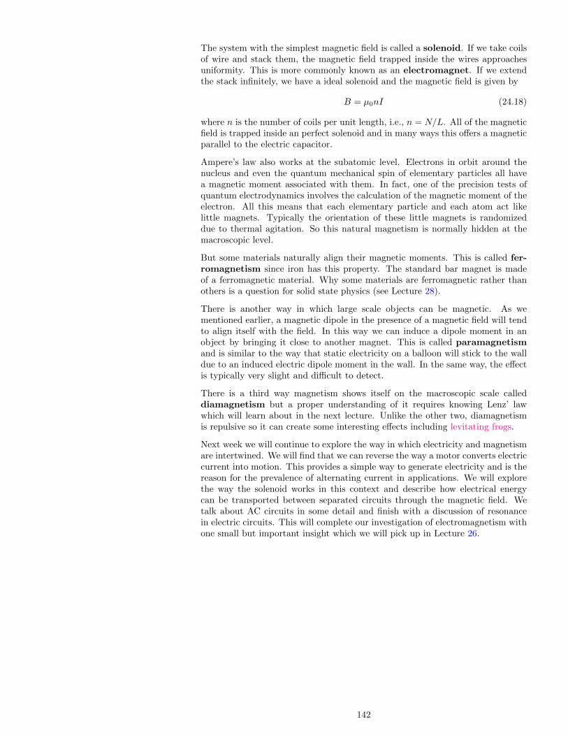
The system with the simplest magnetic field is called a solenoid. If we take coilsof wire and stack them, the magnetic field trapped inside the wires approachesuniformity. This is more commonly known as an electromagnet. If we extendthe stack infinitely, we have a ideal solenoid and the magnetic field is given by

B = µ0nI (24.18)

where n is the number of coils per unit length, i.e., n = N/L. All of the magneticfield is trapped inside an perfect solenoid and in many ways this offers a magneticparallel to the electric capacitor.

Ampere’s law also works at the subatomic level. Electrons in orbit around thenucleus and even the quantum mechanical spin of elementary particles all havea magnetic moment associated with them. In fact, one of the precision tests ofquantum electrodynamics involves the calculation of the magnetic moment of theelectron. All this means that each elementary particle and each atom act likelittle magnets. Typically the orientation of these little magnets is randomizeddue to thermal agitation. So this natural magnetism is normally hidden at themacroscopic level.

But some materials naturally align their magnetic moments. This is called fer-romagnetism since iron has this property. The standard bar magnet is madeof a ferromagnetic material. Why some materials are ferromagnetic rather thanothers is a question for solid state physics (see Lecture 28).

There is another way in which large scale objects can be magnetic. As wementioned earlier, a magnetic dipole in the presence of a magnetic field will tendto align itself with the field. In this way we can induce a dipole moment in anobject by bringing it close to another magnet. This is called paramagnetismand is similar to the way that static electricity on a balloon will stick to the walldue to an induced electric dipole moment in the wall. In the same way, the effectis typically very slight and difficult to detect.

There is a third way magnetism shows itself on the macroscopic scale calleddiamagnetism but a proper understanding of it requires knowing Lenz’ lawwhich will learn about in the next lecture. Unlike the other two, diamagnetismis repulsive so it can create some interesting effects including levitating frogs.

Next week we will continue to explore the way in which electricity and magnetismare intertwined. We will find that we can reverse the way a motor converts electriccurrent into motion. This provides a simple way to generate electricity and is thereason for the prevalence of alternating current in applications. We will explorethe way the solenoid works in this context and describe how electrical energycan be transported between separated circuits through the magnetic field. Wetalk about AC circuits in some detail and finish with a discussion of resonancein electric circuits. This will complete our investigation of electromagnetism withone small but important insight which we will pick up in Lecture 26.

142

Lecture 25

EM Induction and ACElectronicsRead sections 22.1–22.4, 22.7–22.9 and 23.1–23.4

An electrodynamic tether is essentially a huge wire that hangs off a satellite orspace craft as it travels through the magnetic field of the earth. The electrons inthe conductor are free to move and since they are moving through a magnetic fieldthey are pushed by the Lorentz force. Thus a current is induced in the conductor(see Figure 25.1). This way of driving current is called motional EMF and is asimple way (in principle) to extract energy from the earth’s magnetic field.

v

+

+

−−

L

x = vt

Figure 25.1: Motional EMF generated by anelectrodynamic tether

This is an example of a type of electromagnetic induction. We can calculatethis motional EMF by blocking the current flow. As the charges separate in thewire, an electric field forms since the charges are attracted to one another (likea capacitor). This electric field counterbalances the Lorentz force caused by themotion of the charges through the magnetic field. At equilibrium the net voltageis zero, so the voltage induced by the charge separation equals the motion EMFcausing the charge separation. Setting the electric and magnetic forces equal wehave E = vB since the charge cancels from both sides. Using the definition offield potential (23.8), the motional EMF generated in this process must be

Vemf = vBL (25.1)

where L is the length of the wire.

Equation (25.1) is a special case of Faraday’s law of induction:11You might wonder why there is no propor-tionality constant here. The way we havedefined the electric and magnetic constantsin the previous lectures happens to make theproportionality here equal to one.

Vemf = −∆Φmag

∆t(25.2)

In Figure 25.1, the wire sweeps out the area given by Lvt. The magnetic flux cutby the wire is therefore LvtB, which after dividing by t and rearranging gives usequation (25.1).

The negative sign tells us which direction the EMF points and the rule in sum-marized in Lenz’ law:

The magnetic field produced by the current driven by the inducedEMF opposes the change in magnetic flux surrounded by the current.

In Figure 25.1, the current flows up the wire which generates a magnetic field outof the paper behind the wire. This field opposes the field in the highlighted areaconsistent with Lenz’ law.

143

Consider another example in which we have a conducting ring sitting perpendic-ular to a magnetic field (see Figure 25.2). If we shut the field off, current will flowin the wire attempting to restore the field (according to Lenz’ law).

Figure 25.2: Induced EMF in a conducting ring by a changingmagnetic field ∆t =⇒

I

Vemf

Now, consider this question: where are the positive and negative terminals of thiselectromotive force? Answer: there are none—the induced EMF is circular.2 In

2This fact perhaps justifies maintaining thedistinction between EMF and voltage.

other words, when the magnetic field changes, it curls up the electric field!

Perhaps the most important application of Faraday’s law is the electric gener-ator. In principle, a basic generator is a electric motor operating in reverse—seeFigure 24.6. We turn the coil and current flows. Faraday’s law operates herebecause the coil cuts through the magnetic flux. Assuming the coil rotates at aconstant angular speed of ω, the flux within a coil with area A is given by

Φmag = BA cosωt

This assumes the coil is initially perpendicular to the field. Faraday’s law (25.2)tells us that the induced EMF in the coil will be3

3This formula can be verified by using theprojection technique we used in Lecture 12while discussing simple harmonic motion(page 71). It’s easiest if you use a squarecoil. A bit of calculus would be of use here.

Vemf = BAω sinωt (25.3)

This equation is the reason for alternating current in electronics. The sinu-soidal pattern of both voltage and current activates Faraday’s law and allows usto play with the full power of the electromagnetic field.

Vrms

Vpeak

t

Square waveVrms/Vpeak = 1

Vrms

Vpeak

t

Triangle waveVrms/Vpeak = 1/2

Vrms

Vpeak

t

Sine waveVrms/Vpeak =

√1/2

Figure 25.3: Examples of AC voltage patterns and their corresponding RMS values

Technically, alternating current can refer to any repeating pattern of current as inFigure 25.3, but the vast majority of the time we will be considering the sine wavepattern. In the figure I have highlighted the RMS value for the voltage which isa kind of average—a measure of where the voltage is “most of the time”. Theterm RMS stands for root-mean-square which is how it is calculated: take theaverage of the voltage squared then take the square root. This trick eliminatesthe sign of the voltage—the simple average for all three patterns is zero.

Most of the analysis in our AC electronics will be using the RMS value of the ACvoltage. In general, assume the quantities involved are RMS values unless youare otherwise told.

Using alternating current electromagnetic energy can be transmitted betweencircuits that are not electrically connected. Fluctuating current in one wirewill drive current through another wire according to Faraday’s law (25.2). Thisinterconnection of two electric circuits through the magnetic field is called theirmutual inductance. For a wire, the magnetic field drops off according to

144

equation (24.14) so we have to bring the wires close together before this electricalinterference manifests itself.

However, we can concentrate this electromagnetic energy by using solenoids in-stead. This is how the transformer works. Suppose we take a solenoid andwrap another on top of it without connecting them. Since the geometries are thesame, the magnetic flux in one will be the same as the magnetic flux in the other.The current in the primary coil will drive the magnetic field that influences thevoltage in the secondary.

This magnetic field is influenced by the number of coils in the primary accordingto equation (24.18). The amount of voltage induced in the secondary is relatedto its number of coils since Faraday’s law (25.2) applies to each coil and the EMFaccumulates. This means that the voltages are related to the number of coilsaccording to

VsVp

=NsNp

(25.4)

The ratio on the right-hand-side is called the turns ratio. The transformer issaid to “step-up” or “step-down” the voltage depending on whether the turnsratio is greater than or less than one, respectively.

Any change in voltage comes at a cost: the currents are inversely proportional tothe turns ratio. This fact will conserve the overall energy in the system accordingto equation (24.2).

Of course, the magnetic field from a current also induces an EMF back ontoitself. This EMF actually opposes the original current flow and is called backEMF. It’s a kind of natural resistance from the electromagnetic field itself andclosely related to Lenz’ law. What this means is that every circuit has its ownself-inductance. We define the self-inductance of a circuit through the equation

Vemf = L∆I

∆t(25.5)

The self-inductance defines how sensitive the back EMF a circuit is to changes incurrent. In particular, the self-inductance of an ideal solenoid is

L = µ0n2Ad (25.6)

which can be derived by combining equations (24.18), (25.2) and (25.5).

When we talk about a solenoid in an electronic circuit, we use the term inductor.Similar to the way a capacitor requires work to come up to full voltage, theinductor requires work to come up to full current since we are working againstthe back EMF from Faraday’s law. The total work required can be calculatedfrom equation (25.5). It is

W = 12LI

2 (25.7)

This energy is stored in the magnetic field inside the inductor. This parallels theway the energy required to charge a capacitor is stored in its electric field.4

4The parallel is not as exact as it mightlook. For example, see an interesting discus-sion on how to release the magnetic energystored in the inductor (to “discharge” it)here and here.

So far, we have discussed three basic electronic components: the capacitor, re-sistor, and inductor. We now wish to investigate how these three componentswork in AC circuits. But before we do, I would like to introduce you to somemathematical trickery known as phasors.

Typically phasors are introduced as complex numbers, but the important thing toknow is that they are two-component quantities. Essentially we are going to usethe analogy we made in Lecture 12 between uniform circular motion and simpleharmonic motion (see Figure 25.4). We represent our oscillating quantity (i.e.,voltage and current) with a vector that uniformly rotates around a circle. Itsangular speed is ω = 2πf .

145

Figure 25.4: Actually, we have already used phasors: takenfrom Figure 12.2

x(t) = A cos(ωt) v(t) = Aω sin(ωt)

The most important thing to realize from Figure 25.4 is that if any quantityoscillates according to A cos(ωt), then its rate of change also oscillates. Theformula for its rate of change is Aω sin(ωt).

For example, if we run an alternating current through an inductor we expect itto generate an EMF due to its self-inductance by (25.5). If the pattern of thecurrent is I(t) = I0 cos(2πft), then the voltage across the inductor will be

V (t) = (2πfL)(I0) sin(2πft)

The ratio of the RMS values of the voltage and current is called the reactanceof the inductor:

XL =Vrms

Irms= 2πfL (25.8)

This self-inductance means that when an inductor is attached to a high frequencyAC voltage source the resulting current will be small since most of the energy willoscillate in the magnetic field.

A capacitor reacts quite differently to high frequency AC voltage. The faster thefrequency, the faster the charges have to move to keep up according to equation(23.13). Since current is the flow rate of charge we can rewrite this equation as

I = C∆V

∆t

So if the pattern of the voltage is V (t) = V0 cos(2πft), then the current acrossthe capacitor will be

I(t) = (2πfC)(V0) sin(2πft)

Which means the capacitor has a reactance of

XC =Vrms

Irms=

1

2πfC(25.9)

Resistors, capacitors, and inductors are called passive components becausethe magnitude of current and voltage are proportional through equations (24.3),(25.9), or (25.8), respectively.5

5Active components include diodes andtransistors which we will talk about in Lec-ture 28.

Notice that in the case of resistance the current and voltage wave patterns are inphase. But with reactive components, there is a phase shift. For inductors, thevoltage is tied to the change in the current. So the voltage peaks at the initial riseof the current and drops to zero when the current hits its peak. There is a phaseshift between the two wave patterns: the voltage is 90 in front of the current.

For a capacitor, the current is tied to the change in voltage. So the current is90 in front of the current. One way to remember the phase shifts for the two

146

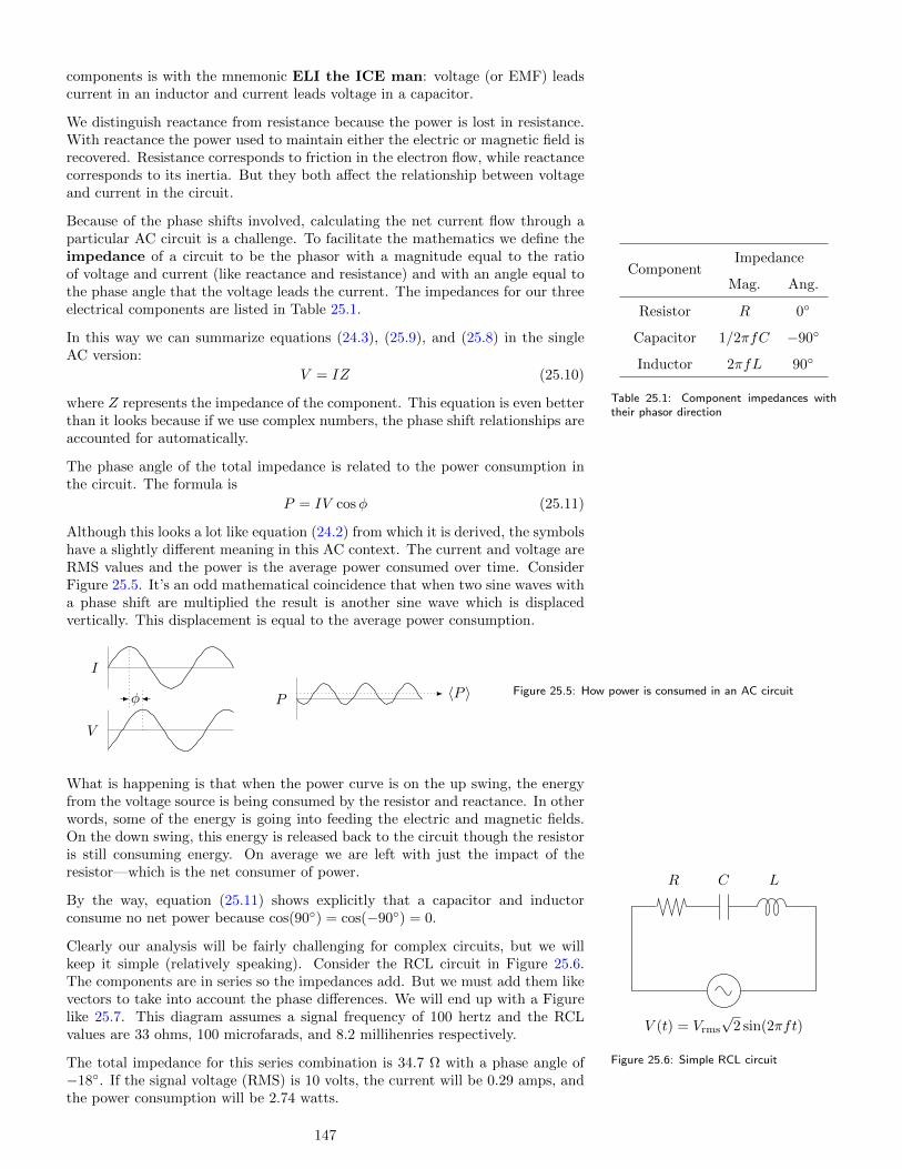
components is with the mnemonic ELI the ICE man: voltage (or EMF) leadscurrent in an inductor and current leads voltage in a capacitor.

We distinguish reactance from resistance because the power is lost in resistance.With reactance the power used to maintain either the electric or magnetic field isrecovered. Resistance corresponds to friction in the electron flow, while reactancecorresponds to its inertia. But they both affect the relationship between voltageand current in the circuit.

Because of the phase shifts involved, calculating the net current flow through aparticular AC circuit is a challenge. To facilitate the mathematics we define theimpedance of a circuit to be the phasor with a magnitude equal to the ratioof voltage and current (like reactance and resistance) and with an angle equal tothe phase angle that the voltage leads the current. The impedances for our threeelectrical components are listed in Table 25.1.

ComponentImpedance

Mag. Ang.

Resistor R 0

Capacitor 1/2πfC −90

Inductor 2πfL 90

Table 25.1: Component impedances withtheir phasor direction

In this way we can summarize equations (24.3), (25.9), and (25.8) in the singleAC version:

V = IZ (25.10)

where Z represents the impedance of the component. This equation is even betterthan it looks because if we use complex numbers, the phase shift relationships areaccounted for automatically.

The phase angle of the total impedance is related to the power consumption inthe circuit. The formula is

P = IV cosφ (25.11)

Although this looks a lot like equation (24.2) from which it is derived, the symbolshave a slightly different meaning in this AC context. The current and voltage areRMS values and the power is the average power consumed over time. ConsiderFigure 25.5. It’s an odd mathematical coincidence that when two sine waves witha phase shift are multiplied the result is another sine wave which is displacedvertically. This displacement is equal to the average power consumption.

I

V

φ P 〈P 〉 Figure 25.5: How power is consumed in an AC circuit

What is happening is that when the power curve is on the up swing, the energyfrom the voltage source is being consumed by the resistor and reactance. In otherwords, some of the energy is going into feeding the electric and magnetic fields.On the down swing, this energy is released back to the circuit though the resistoris still consuming energy. On average we are left with just the impact of theresistor—which is the net consumer of power.

By the way, equation (25.11) shows explicitly that a capacitor and inductorconsume no net power because cos(90) = cos(−90) = 0.

Clearly our analysis will be fairly challenging for complex circuits, but we willkeep it simple (relatively speaking). Consider the RCL circuit in Figure 25.6.The components are in series so the impedances add. But we must add them likevectors to take into account the phase differences. We will end up with a Figurelike 25.7. This diagram assumes a signal frequency of 100 hertz and the RCLvalues are 33 ohms, 100 microfarads, and 8.2 millihenries respectively.

V (t) = Vrms

√2 sin(2πft)

R C L

Figure 25.6: Simple RCL circuitThe total impedance for this series combination is 34.7 Ω with a phase angle of−18. If the signal voltage (RMS) is 10 volts, the current will be 0.29 amps, andthe power consumption will be 2.74 watts.

147

Figure 25.7: Phasor calculation

ZR = 33.0 Ω

ZC = 15.9 Ω

ZL = 5.15 Ω

Ztot

Notice that the voltage across the RCL components are 9.51, 4.59, and 1.48 voltsrespectively. Clearly these numbers do not add back to the 10 volts from thesource. Remember that these individual voltages are the RMS values across thecomponents. If we were to account for the phase differences (the picture wouldlook just like Figure 25.7) we do get back to the original 10 volts.

One important aspect of a circuit like Figure 25.6 is that the current flow isdependent on the frequency of the source voltage. When the frequency is high,the inductor has a high reactance which blocks current. At low frequency, thecapacitor has high reactance which blocks the current. In the middle, we have aspike in current flow. This is an example of electrical resonance (see Lecture 12).The inductor acts like the mass, the capacitor acts like the spring, and the resistoris the damping force. Once the current reaches its steady state, the capacitor andinductor require no more power: the energy merely oscillates between the electricand magnetic fields. This leaves the resistor as the only source of impedance. Theformula for the resonant frequency of the series RCL circuit is:

f0 =1

2π

1√LC

(25.12)

The phase shift also depends on the frequency. A plot of the power consumptionof our circuit from Figure 25.6 is the upper plot of Figure 25.8. If we reduce theresistance by a factor of ten we get the plot underneath it.

P

f

R = 33 Ω

f0

P × 10

f

R = 3.3 Ω

f0

∆f

Figure 25.8: Resonance in the RCL circuit

The reduction in resistance increases the current flow which increases the overallpower consumption of the circuit. But it also sharpens the resonance peak. Therange of frequencies for which the power exceed half of its maximum value iscalled the bandwidth of the circuit. For this RCL circuit the bandwidth is

∆f = R/L (25.13)

A better measure of the sharpness of the peak will normalize for the resonantfrequency it surrounds. This is called the quality factor for the circuit. In thisexample we have

Q =f0

∆f=

1

R

√L

C(25.14)

This Q-factor is important if we are trying to target a particular frequency withour resonant circuit (in a radio, for example).

Next week we will tie up one last loose end in electromagnetic theory. Withthis last piece, we will see that light is an electromagnetic wave. This will openup the whole non-visible spectrum of frequencies for investigation: radio waves,microwaves, gamma rays, etc. The dark side of this story is that the new theoryis in conflict with Newton’s laws of motion. Ultimately the resolution is foundin Einstein’s special theory of relativity. We will end up redefining space, time,mass, momentum and energy before we are done. Finally, we will touch on howrelativity theory affects our other long-range force: gravity—which will requirethe general theory of relativity.

148

Lecture 26

Electromagnetism andRelativityRead sections 24.1–24.4 and 28.1–28.7, review Lectures 5, 7, and 8

There is a problem in what we have developed so far—the problem is in Ampere’sLaw (24.13). It only works if the flow of current is continuous. To see why,consider what happens when we charge a capacitor. If we draw the circle Aaround the incoming current, Ampere’s law tells us that the magnetic field curlsaround the wire (see Figure 26.1). What Ampere’s law does not tell us is whichsurface to use to determine I. No current pierces the dashed surface indicated.Using this surface, we could conclude that there is no magnetic curl at all. A

I

∆q

∆Φele

Figure 26.1: Ampere’s law needs Maxwell’scorrection

This inconsistency went unnoticed until Maxwell offered a solution in 1861. Phys-ically, we know that if current is flowing into a region without coming out, chargemust be piling up somewhere. In Figure 26.1 the charge is piling up on the plateof the capacitor. Gauss’ law (23.4) tells us that the electric flux is increasing too.Although current doesn’t pierce the dashed surface, this flux does. So Maxwelladded a correction to Ampere’s law by assuming that a changing electric flux willalso curl the magnetic field:1

1Don’t worry: I know this formula is ugly. Ionly include it for completeness. We won’thave to use it in this class.

∑loop

Bt∆s = µ0ε0∆Φele

∆t(26.1)

I like to call this magnetoelectric induction to emphasize an analogy toFaraday’s law (25.2).2 In Faraday’s law we see that a changing magnetic field

2Maxwell called the term ε0∆Φele/∆t onthe right displacement current.

can create an electric one. In Maxwell’s correction (26.1) we see that a changingelectric field can create a magnetic one.

Maxwell took this one step further. Prior to Maxwell, physicists had suspecteda connection between light and electromagnetism. He was able to show that hisadditional term implied that the electromagnetic field could act as a mediumsupporting a wave. The energy of the wave resonates back and forth between theelectric field and the magnetic field, like an RCL circuit without the circuitry.

He calculated the speed of this wave as

c =

√1

µ0ε0= 2.998× 108 (26.2)

which is the speed of light.3 So with one minor modification Maxwell completed3Equation (26.2) shows that Maxwell’s cor-rection (26.1) is on the order of 1/c2.We will see in a bit that this should beconsidered a relativistic correction.

electromagnetic theory and derived a wave theory of optics. For this, theseequations are now collectively called Maxwell’s equations.

149

In general, the energy density of the electromagnetic field is given by

u = 12 (ε0E

2 +B2/µ0) (26.3)

for which equations (23.15) and (25.7) are special cases. Notice how the energyis proportional to the square of the field magnitude similar to (12.9).

But for the special case of electromagnetic waves, the electric and magnetic fieldsare perpendicular to each other. In addition, the magnitude of the fields arerelated by E = cB. The oscillation of the fields are transverse and they areperpendicular to flow of energy.4 In fact, the intensity of the radiation is given

4The polarization of the wave is usuallydefined by the direction of the electric field.

by5

5Compare this intensity calculation withthat in Lecture 18.

I = P/A = cu = 12cε0E

2 (26.4)

The factor of one-half is there because the electric field is oscillating. The valueof E represents the amplitude or peak value of the wave.

a

Figure 26.2: Radiation pattern from acharge accelerating to the right (or left)

This electromagnetic radiation occurs whenever a charged particle accelerates.Most of the energy is distributed perpendicular to the direction of the accelerationas in Figure 26.2. The total power radiated is given by Larmor’s formula:

P =a2q2

6πε0c3(26.5)

where q is the magnitude of the charge and a is its acceleration. It is this formulawhich predicts the death spiral of the electron that we mentioned in Lecture 22.

One of the most dramatic consequences of Maxwell’s discovery of electromagneticwaves was the opening up of the entire non-visible spectrum. Shortly afterwardHertz confirmed this by generating and capturing radio waves which sit on thelower frequency end of visible light. High energy sources like quasars and nuclearradiation produce EM waves that sit on the higher end of the frequency spectrum.

By equation (26.5) any wire with alternating current will generate EM radiation.Similarly, any wire will react to EM radiation. This is the basic physics behindany wireless technology (radio, TV, router, cell phone, etc.) Typically, theelectromagnetic fields associated with EM waves are so feeble that some sortof amplification is required to pick up these signals. This is why sometimes alightening strike will cause electrical interference. The use of frequency bands areregulated to avoid having people interfere with one another’s electronics.

Since the acceleration of the charges is related to the frequency squared (cf.Lectures 25 and 12), the power radiated increases with the fourth power of theAC frequency. This is why the sky is blue. As light from the sun passes throughthe atmosphere, it causes the atoms of the atmosphere to oscillate back and forth.This motion causes EM waves to re-radiate—perpendicular to the motion of theoriginal radiation. This effect occurs at the highest end of the spectrum most,which is the blue end of the solar spectrum.

Clearly we could go much deeper into the study of electrodynamics, but here westop. We now turn to discuss special relativity. Although relativity was uncoveredthrough the study of electromagnetism,6 Einstein saw that the consequences were

6Einstein’s paper in 1905 was titled “On theelectrodynamics of moving bodies”.

not just isolated to electromagnetic theory but stuck at the very foundation ofNewtonian mechanics.

Most explanations of relativity start with a light clock and so will ours. Imaginea thin tube with mirrors on the ends in which a light pulse is bouncing backand forth. Orient it vertically and allow it to move to the right with constantspeed. The trajectory of the light pulse as it bounces from bottom to top formsa triangle as in Figure 26.3. This innocuous looking diagram is the Trojan horseof relativity. All of our troubles begin with the following argument.

ct

ct0

vt

Figure 26.3: Light clock and time dilation

Light travels with constant speed, so the height of the clock is related to the timeit takes for light to travel up the clock by ct0. But if the clock is moving to the

150

right, the trajectory of the light runs up the hypotenuse of the triangle in Figure26.3. The distance it moves to the right is vt where t is the time it takes the lightpulse to hit the top of the clock. Clearly t > t0. In fact, we have

(ct)2 = (ct0)2 + (vt)2 (26.6)

which can be rewritten ast = t0/

√1− v2/c2 (26.7)

Which is called the time dilation formula because the moving clock ticks slower.

Hopefully you are saying to yourself, “Slow down—how can such a simple set-up lead to such a sweeping statement about the nature of time itself?” Thereis one thing that makes this argument special: we are using light. If this werea bullet from a gun, the speed in the vertical direction would be unaffected bythe horizontal motion. The two velocities would add (as vectors). This is anapplication of the principle of relativity: the bullet would take the same amountof time to cross the distance regardless of the horizontal motion.

But this is light—which only moves at the speed of light. Now, the same is trueof sound: it travels at a certain speed through to its medium (air). But light isdifferent because it always travels at the speed of light no matter what. This iswhat makes the Michelson-Morley null result so important. It shows that light isnot like a sound wave.

Though many physicists realized that something was up, Einstein saw the heartof the issue. If light speed is the same no matter the frame of reference used,then the principle of relativity forces us to conclude that time is an individualphenomena. My time is not the same as your time—though they are relatedthrough equation (26.7).

Suppose we span the distance L0 = vt with a stick. From the perspective of anobserver moving with the clock, this stick is traveling the opposite direction withthe same speed so L = vt0. Since the times are related via equation (26.7), themeasured lengths are related via

L = L0

√1− v2/c2 (26.8)

Since L < L0, this is called length contraction. In relativity, motion shrinksspace and slows down time.

An objection may occur to you. If I think the moving ruler is shorter, won’t themoving observer think my ruler is longer? This contradicts equation (26.8). Theresolution is that the moving observer will not think my measurement is valid dueto another relativistic phenomena called desynchronization.

Whenever we measure the length of an object in motion, we have to make surethat we mark the edges at the same time. But moving observers disagree onwhich events are simultaneous. Suppose we flash a light from the exact centerof our ruler. We wait for the beams to bounce and return to center. Based onthis duration and the speed of light, we calculate the length. But the movingobserver sees something like Figure 26.4. The back end of the ruler runs intothe light beam at event A. The front end of the ruler is running away and eventB occurs later. But I claim that the length of the ruler is the distance betweenthese two points. The moving observer thinks, “Of course you think your ruler islonger—you are cheating. Your ruler is actually shorter by (26.8), but the timelag of vL/c2 in your measurements overcompensates by a factor 1/(1− v2/c2).”

A

B

t

Figure 26.4: Clocks separated in space aredesynchronized

All of these effects are summarized in the Lorentz transformation which trans-lates the space-time measurements between moving observers. If an observer ismoving with velocity v relative to you, her measurements are related to yoursaccording to

x′ = γ(x− vt) t′ = γ(t− vx/c2) (26.9)

151

where γ = 1/√

1− v2/c2. This is sometimes called the Lorentz factor and isthe hallmark of relativity. We can neglect relativistic effects when γ is close toone. Even when v is 10% the speed of light, γ is within 0.5% of one.

These equations are fundamental and affect every other calculation in mechanicsyou have learned so far. In particular, the velocity of an object as measured inthe moving frame will be

u′ =∆x′

∆t′=

γ(∆x− v∆t)

γ(∆t− v∆x/c2)=

u− v1− uv/c2

Without relativity, we would simply subtract the motion of the observer from ourmeasurements like u′ = u−v, but the desynchronization effect in the denominatorchanges how the velocity measurements interact.

This is also one of the ways we can see why no object can move faster than light.If we start with an object moving at velocity v and increment the velocity by anamount u (less than the speed of light), the final speed is given by

u′ =u+ v

1 + uv/c2(26.10)

which will always be less than light speed.7

7Here’s the proof. Both u and v are lessthan c. Thus c − u and c − v are bothgreater than zero and so is their product.Rearranging this inequality we can say

c2(1 + uv/c2) > c(u+ v)

Rearrange again and the conclusion follows.

One hidden consequence of equations (26.9) is that between any two events, thecombined quantity

I = (c∆t)2 −∆x2 (26.11)

is the same for both observers.8 This space-time interval is truly the best8The converse is also true: equations (26.9)are the only linear combinations which pre-serve this quantity.

representation of how space and time are united and intertwined in relativitytheory. Investigating the geometry associated with this interval offers a wayof viewing the theory that is illuminating and mitigates the feeling of a cosmicconspiracy that time dilation, length contraction and desynchronization generate.

Since velocities don’t work the way we are used to in relativity, is it any surprisethat momentum and energy don’t either? The most egregious situation is thatthe conservation of our friend mv is no longer invariant. For example, if the totalmomentum is zero in the center of mass frame, it will not be conserved in the labframe because of the way velocities combine in equation (26.10).

Fortunately, it can be shown that the conservation of γmv is invariant.9 This is9The proof is straightforward, but a bitlaborious. You will need to know that

γv′ = γuγv [1 + uv/c2]

called the relativistic momentum and clearly reduces to the classical definitionof momentum when v c. However, in order for relativistic momentum to beconserved we must also have γm conserved. This may seem odd until one runsthrough the classical version of this argument and notices that it requires m tobe conserved. So in order for this relativistic argument to work we must redefineboth momentum and mass.

The quantity γm is frequently called relativistic mass, though this usage hasgone out of favor.10 The main reason is that guessing at a relativistic formula by

10Although in his physics lectures, Feynmanmakes the claim that all of relativity canbe derived from this one formula. Actually,the idea of relativistic mass goes back toEinstein himself. It’s pretty easy to starta flame war on physics related websitesnowadays just by bringing up the topic.

simply replacing m with γm in most classical formulas won’t work. The preferredapproach is to multiply this quantity by c2 and call it relativistic energy anduse m only to refer to the mass of an object measured from rest (i.e., its restmass). Since γmc2 is in units of energy, we are okay to call it this but there isan even better reason.

Using the binomial theorem (1.3) we have

γ = (1− v2/c2)−1/2 ≈ 1 + 12v

2/c2 (26.12)

This is a useful approximation to be aware of it its own right. But is also meanswe can say

E = γmc2 = mc2 + 12mv

2 + . . .

152

The first term is a constant and is called the rest energy of the particle since itdoesn’t go away even if the particle is at rest. The second term is our friend kineticenergy. The remaining terms are relativistic corrections to this kinetic energyformula.11 A second verification of this approach is possible by calculating the

11If you are interested, the next term hap-pens to be 3

8mv4/c2.

work required to relativistically accelerate a particle from rest. If we use p = γmv,then the total work done on the particle is12

12Unfortunately, I know of no non-calculustechnique of deriving this equation. If youthink of one, let me know!

KE = (γ − 1)mc2

which is the same way we derived the 12mv

2 formula in classical mechanics.

We continue to call a collision elastic if it conserves kinetic energy. But noticethat in relativity the total energy γmc2 is conserved even in inelastic collisions.

Consider two identical particles that are flying toward one another with equal andopposite velocities. Suppose they each are moving fast enough to have a Lorentzfactor of 3

2 so the total energy of the system is 3mc2. If they collide and stick(completely inelastic collision), the composite still has this energy. But now it isat rest (net momentum is zero) with a Lorentz factor is one. It follows that therest mass of the composite is 3m—the mass of the object continues to hold theincoming kinetic energy.

The reverse of this process works too. This connection between mass and energyis completely unexpected in classical mechanics and is one of the reasons whyE = mc2 is so famous. We can calculate the energy locked in the nucleus of theatom by comparing the mass of the composite atom with the mass of its parts.Multiply this difference by c2 and the number of atoms in a kilogram of uraniumand you end up with a very big number.

Occasionally in relativity problems you know the energy and momentum of aparticle and need to determine the velocity. One shortcut to use is

Ev = pc2 (26.13)

which completely skips the need to deal with γ in the calculation.13 Another13This implies that the energy and momen-tum of a light pulse are related through E =pc. Plugging this into the next equation(26.14) yields m = 0. This is why we saya photon has zero rest mass even though aphoton is never actually at rest. Reversingthe argument works too, so anything with“zero rest mass” can only move with thespeed of light.

useful connection between these concepts is

E2 − p2c2 = m2c4 (26.14)

This equation is more important than it looks. This is because it parallels equation(26.11) with energy connected to time and momentum connected to space. If wewere to dive down the rabbit-hole, we would combine energy and momentum intoa single four-vector called four-momentum. Similar to the way distance andduration are “projections” of the space-time interval, the energy and momentumof a particle are the “projections” of this relativistic four-momentum. They aredilated, contracted, and mixed via the Lorentz transformation (26.9) just likespace and time.

Though we have covered a lot, one obvious gap is left: Newton’s second law. Thegap is not as critical as it seems because most applications of relativity involvethe analysis of collisions for which energy and momentum are sufficient. On theother hand, the means of relativistically correcting a particular force law is notan easy problem.

But we already know that electromagnetism is a relativistic theory. One insightthat relativity brings to electromagnetism is that the electric force and the mag-netic force are not just intertwined, but can be considered as “projections” of afour-dimensional electromagnetic force. In a similar way to how energy and mo-mentum are “shadows” of a relativistic four-momentum, the electric and magneticforces are the “shadows” of electromagnetism on time and space, respectively.14

14The two forces also mix together in for-mulas similar to the Lorentz transformation(26.9). This implies that a force we considermagnetic in one frame may be considered tobe electric in another. This fact was whatEinstein originally considered as the maintheoretical support for relativity.Though a bit more complicated because we are talking about combining two

vectors into some four-dimensional tensor, this approach radically simplifies theequations of electromagnetism.

153

We have already made the point that fundamentally all the other macroscopicforces (except gravity) are electromagnetic in origin. So in principle, all that’sleft is a lot of calculations.15

15This is extremely unfair, of course. Thecomplexities of how electromagnetism man-ifests itself as elastic, friction, tension, andother forces depends upon a perfect under-standing of the nature of matter. Until thatproject is done, this statement is untrue. Then there is gravity. One key element of any relativistic force law is that its speed

of influence cannot exceed the speed of light. So we know right away that Newton’slaw of gravity (6.3) is wrong. Einstein had the fundamental physical insight in1907 to solve the problem. It took him another eight years to struggle throughthe math and find the correct theory which we call general relativity.16 This

16This branch of mathematics is now knownas differential geometry.

was an experience he never forgot and is why he wrote the following statement ina 1943 letter that may seem incredible to you:

Do not worry about your difficulties in mathematics. I can assure youmine are still greater.

Einstein’s physical insight is now called the equivalence principle and is thesimple recognition that a reference frame accelerating under the influence ofgravity (in free-fall) is inertial. Mathematically this is because the mass inNewton’s second law (5.1) is the same as the mass in the law of gravity (6.3). Soeverything accelerates together in tandem. Einstein saw that this special propertyallows one to generalize the principle of relativity to include frames in free-fall.

Here’s the trick: we know how to correct Newton’s laws in the freely fallingframe—use special relativity. What we need to know is how to transform thesecorrections out of the free-fall frame to one on the ground. The answer is to replacethe space-time interval in equation (26.11) with the Schwarzschild metric:17

17Confession: This is the basic idea, butI’ve cheated here. We need to take intoaccount the polar coordinates used to derivethis formula by replacing x with r and weneed to add a couple of terms. For the fullmeal deal see Wikipedia.

I(r) =

(r − rsr

)(c∆t)2 −

(r

r − rs

)∆x2 (26.15)

where rs = 2GM/c2 and is called the Schwarzschild radius. This length isthe characteristic distance in which general relativistic effects are important. Forthe Sun it is three kilometers which is negligible on an astronomic scale. TheSchwarzschild radius represents the distance at which light is captured by anobject and therefore represents the effective radius of a black hole. A black holeneed not be massive: it must be very dense. If we could compress the mass of theEarth below a radius of nine millimeters, general relativity would take over andit would collapse into a black hole.

For any stationary clock ∆x = 0 and the space-time interval equals (ct0)2 wheret0 is the proper time measured by the clock. Because of the factors in theSchwarzschild metric (26.15), a stationary clock in a gravitational well will tickslower than one in deep space (gravitational time dilation). We have

t0 = t

√1− 2GM

rc2≈ t− GM

rc2(26.16)

This effect is directly confirmed in the delay of radar beams bounced off Venusand in gravitational red-shift. It can also be used to see that the speed of lightappears to slows down as it approaches the Schwarzschild radius of a black hole.18

18Any object falling into a black hole willappear to slow down. In fact it will neverappear to cross the Schwarzschild radius.From the object’s point of view there isnothing unusual—it just falls, but the out-side world never sees anything after this lineis crossed. This is why this radius is alsocalled the event horizon of the black hole.

This change in speed can deflect light (like refraction through variable media—seeLecture 20). This prediction and its dramatic confirmation in the eclipse of 1919launched Einstein to world-wide fame.

I’ve left a lot out (obviously) including gravitational waves, cosmology, and howthis is all related to “curved spacetime”. For a few more insights review the endof Lecture 11 and 13, but here we must stop.

Next week we make a complete shift in gears to talk about quantum mechanics.We have already discussed (Lectures 16 and 22) how cracks in our understandingof the very small began to appear around 1900. We will talk about how these

154

issues were resolved over the following 50 years through an understanding of thewave nature of matter. We will also touch on the difficulties and the ultimatesuccess of creating a quantum theory of electrodynamics.

155

156

Lecture 27

Quantum MechanicsRead sections 29.1–29.6 and review Lecture 22

We’ve already discussed some of the reasons why physicists around 1900 werebeginning to witness the breakdown of classical physics. Shortly after relativitymade us adjust our understanding of the fast and energetic, a much larger attackwas made on our understanding of the very small. If you thought relativity wasmind-blowing, you might want to sit down now.

In Lecture 22 we discussed how Planck and Einstein were driven by experi-ment to postulate a particle theory of light (in flat contradiction to classicalelectromagnetism). The energy relationship for the photon is given in equation(22.2) as E = hf where f is the frequency of the light. Einstein showed howthis relationship could make sense out of the ultraviolet catastrophe and thephotoelectric effect.

The next step down the road to quantum mechanics was taken in 1924 by Louisde Broglie. His argument was basically: if photons have both wave and particleproperties, then maybe electrons do too. Since the momentum of a photon isgiven by p = E/c and fλ = c for any wave, we have p = h/λ for the photon.He postulated that the electron (and any other material particle) must have anassociated wavelength of

λ = h/p (27.1)

This is known as the de Broglie wavelength of the particle and characterizesits matter wave.1

1Though “matter field” might be a moreappropriate term.At the time, understanding the structure of the atom was the hot topic of the

day. De Broglie’s hypothesis made sense out of some of the results seen at thetime. We will return to this topic in the next lecture. More direct evidence forthe wave nature of matter is available now in neutron diffraction experiments andthe electron double-slit experiment.

EFigure 27.1: Quantum tunneling through a potential energybarrier

One important consequence of the wave nature of matter is quantum tunneling.Consider Figure 27.1. A classical particle with kinetic energy E approaches apotential energy barrier of twice this energy. Classically, we expect the particleto “bounce” off of this barrier. However, a wave will propagate into such a barrierthough with exponentially decreasing amplitude we called this “attenuation” in

157

Lecture 21. If the barrier is small enough, there may be enough amplitude leftfor a small amount of this wave to be transmitted through the barrier.

This is the explanation behind natural radioactivity. The protons are boundtogether by the strong nuclear force (see Lecture 29) which creates a potentialwell for the nucleus. But outside the nuclear range, the protons are repelled bytheir electrostatic repulsion. This combination of the forces produces a barrierthrough which, occasionally, some of the nuclear content escapes.

Overall, De Broglie’s theory is suggestive but incomplete. The Schrodingerwave equation published in 1926 is what we seek:

− ~2

2m

∂2ψ

∂x2= (E − V )ψ (27.2)

where ~ = h/2π. This form of the equation assumes the potential energy V isconstant so the physical system is in a standing wave mode—like a stable atom.The one-dimensional solution to this equation is

ψ = A cos(±kx+ φ) with ~k =√

2m(E − V ) (27.3)

unless E < V in which case the solution is

ψ = A exp(±kx+ φ) with ~k =√

2m(V − E) (27.4)

These are the formulas used to generate Figure 27.1. These standing wavesoscillate with a frequency f = E/h.

By its very nature, a wave is extended in space. It is possible to “localize” thesewaves by combining them with different but similar wavelengths (similar to theFourier analysis in Lecture 19). This means that for waves there is an inverserelationship between the position and wavelength. But the wavelength of ourmatter waves is connected to the momentum of the particle via (27.1). TheHeisenberg uncertainty principle summarizes this relationship as

(∆x)(∆p) ≥ ~/2 (27.5)

The uncertainty principle shows that identifying the exact trajectory of a quantumparticle is doomed to failure.2 The more we localize the particle, the greater the

2Although there is an interesting approachto quantum mechanics by David Bohmwhich claims to do just that.

uncertainty in its momentum. In other words, the more we know about where itis, the less we know about where it will be.

So, in quantum mechanics the matter wave is primary. But what exactly is ψ?Some insight into this question can be gained by revisiting the photoelectric effect.The intensity of the radiation is

I = nhf/t

This is simply the total energy per photon (hf) multiplied by the number ofphotons per second (n/t). This is the particle viewpoint. From the standpointof electromagnetism, the intensity is given by equation (26.4). Setting these twoequations equal to each another yields

nhf/t = 12cε0E

2

Remember that E in this case represents the peak value of the electric field. Asthe photon is related to the electromagnetic field, so the electron is related toits matter wave. In other words, it seems reasonable to assume that the squareof the wave amplitude is proportional to number of particles present. If we aretalking about a single particle, then this value must represent the probability offinding the particle at that location in an experiment. In symbols,

ρ ∝ ψ2 (27.6)

158

where ρ is the probability density of locating the particle at this point in space.Of course, the sum of all these probabilities must be one.

We will explore how the matter wave works in the context of the atom in thenext lecture. We will also get a hint of how quantum mechanics provides physicalfoundation for chemistry and solid state physics. But before we do, an obviousquestion has probably occurred to you. What about relativity? Oddly enough,there are significant conceptual difficulties in building a relativistic quantumtheory. It took physicists 20 years to untangle this Gordian knot and a trioof men (Tomonaga, Schwinger, and Feynman) received the Nobel Prize in 1965for it.3

3Feynman’s Nobel Lecture is an interestingrecounting of some of his journey to unlock-ing these mysteries.

Quantum field theory (QFT) is the result of combining quantum mechanicsand special relativity. In both there is a standard recipe for “graduating” orgeneralizing our classical models.

In special relativity we replace our notions of space and time with space-time andrecognize that both distance and duration are merely components of the space-time interval between the two events. In addition, pairs of mechanical quantitiesare combined in an analogous way—in particular, energy and momentum arerelated according to E2 = p2c2 + m2c4 (26.14) which replaces the Newtonianrelationship KE = p2/2m.

In quantum mechanics we replace the notion of an elementary particle withits “wave-function” ψ(x) which can be used to calculate all of the mechanicalquantities related to this quantum particle. In particular, the momentum of theparticle is related to the slope of the wave and the energy is related to its rate ofchange. In symbols:

p(ψ) = −i~∂ψ∂x

E(ψ) = i~∂ψ

∂t(27.7)

Starting fromp2/2m = KE = E − V

yields Schrodinger’s equation (27.2).

The most natural combination of these two recipes starts with the relativisticequation (26.14) and imposes the quantum recipe to yield

1

c2∂2ψ

∂t2− ∂2ψ

∂x2+m2c2

~2ψ = 0 (27.8)

which is now known as the Klein-Gordon wave equation. However, this equationcan be shown to yield negative probabilities for the location of the quantumparticle. This makes interpreting this probability density problematic.

The correct conclusion is that there is no such thing as a quantum field theory fora single particle.4 The reality is that the analysis of any high energy system must

4It seems almost irreverent to skip Dirac’stheory of the electron here. But it is truly alogical sidebar to our main point. In a way,Dirac exploits a loophole in the previouslogic which delays but in the end does notdeny the final conclusion. Of course we needDirac’s electron (i.e., the electron is a spinorfield), but not as a motivation for QFT.

take into account the possibility of secondary creation and annihilation events.In quantum field theory, every problem is a many-body problem. We now knowhow to deal with that (given some reservations)—we have Feynman diagrams.

Space (x)

Tim

e(t

)

Figure 27.2: A typical Feynman diagram

A typical Feynman diagram looks like Figure 27.2. This is a space-time diagramwith time flowing up the page. The lines represent electrons and the squigglyline is a photon. The black dots at the beginning and end are the actual eventsmeasured in the lab. The white dots in the middle are called “virtual” in thesense that they are not actually observed—the photon exchange is unseen so it iscalled a virtual photon. In quantum field theory, the electromagnetic force ismediated by the exchange of these virtual photons.

Quantum electrodynamics (QED) is the application of quantum field theoryto the electromagnetic force. The photon is governed by Maxwell’s equations andthe electron is described by the formula discovered by Dirac in 1928. Feynman

159

calls it the “crown jewel” of physics and it is the most accurate physical theoryin history—confirmed by experiment within ten parts per billion.

The nice thing about these Feynman diagrams is that you can actually see theelectrons exchanging the photon. In fact, the diagram is so suggestive, it isimportant to emphasize what it is not. It does not represent the actual interactionbetween the electrons—it is a book-keeping tool used to calculate the interaction.The diagram represents a whole class of similar diagrams with the unobservedvirtual events located in different places. Truly anything goes as long as theinitial and final events are the same.

Each Feynman diagram is used to calculate a complex number with an angleproportional to the total action of the diagram (using the Lagrangian from clas-sical mechanics). Those diagrams representing situations far from the classicalprediction typically cancel out. In this way, Feynman found justification for theclassical principle of least action. The diagrams also show us a practical methodof correcting our classical predictions by including those diagrams close to theclassical result.

This correction is more difficult than it may appear. Simply calculating theprobability involved in one electron traveling from point A to point B involves aninfinite number of diagrams (see Figure 27.3).

Figure 27.3: The foremost rule of quantum field theory:anything goes as long as you don’t get caught + + · · ·

This shows that the bare electron is always surrounded by a cloud of virtualparticles like groupies. The electron we measure in the lab is actually this cloud—one never sees a naked electron.

Figure 27.4: Anything goes—including traveling backward intime

Electron

=

Positron

One surprisingly simple consequence of these diagrams is that it is easy to seehow QFT predicts the existence of anti-matter. Consider the pair of diagramsin Figure 27.4. The one on the left represents an electron that emits a photonthen later absorbs and incoming one. But this is equivalent to the other diagramon the right with this order reversed. But what is going on in the middle? Theelectron is going backward in time.

From a technical standpoint, these two diagrams are indistinguishable. You can’thave one without the other. Feynman interpreted the time-traveling electron asthe positron.5 Look at the second diagram a bit closer. The incoming photon on

5The positron was discovered by Carl An-derson in 1932. It has all the properties ofthe electron except with a positive charge.

the right splits into two particles—the one on the right is the outgoing electron.The one on the left is the backward traveling electron. But in the lab we wouldcall this the creation of a matter-antimatter pair, one electron and one positron.Later in time, the positron strikes and annihilates the incoming electron. Thisleaves the outgoing photon as the byproduct. In this way Feynman explained theexistence of antimatter and why every particle has an antimatter twin with thesame mass. Simple.

In fact, we can even draw Figure 27.5. This diagram represents the virtual creationthen annihilation of an electron-positron pair. Note that there are no incoming

160

or outgoing particles. This diagram shows that even the vacuum is full of a seaof virtual matter-antimatter pairs. This is the source of the so-called zero-pointenergy of the vacuum. In quantum field theory even the vacuum is a many-bodyproblem!

Figure 27.5: An oyster diagram—the vac-uum is not empty

One of the most important consequences of quantum field theory is that everyquantum particle falls into one of two categories: fermions or bosons. Bosonsare the exchange particles in our Feynman diagrams: they can be absorbedand emitted by fermions and mediate the interaction between them. Fermionsrepresent the “hard” particles which form into atoms and all the matter we see.Fermions obey the Pauli exclusion principle which states that no two identicalfermions can exist in the same quantum state. There is a natural “repulsion”between them which gives matter its stability. On the other hand, bosons aregregarious: they have a propensity to collect into the same state. This collectivebehavior is why they appear classically as force fields since they work together toproduce a net interaction measurable on a macroscopic scale.

This also helps to explain how a laser works. In a typical laser the medium isdesigned to support the emission of photons. Usually this is done by “pumping”electrons into a high energy state. The electrons each radiate this energy as aphoton in order to return to a lower energy state. The lasing material must beable to support the electrons in this unstable position for a relatively long timeframe (a few nanoseconds).

The laser begins with one photon. The presence of this photon induces the nextphoton to be aligned with itself because of this “gregarious” nature of bosons. Puta couple of mirrors on the end and as long as there are electrons to generate thephotons, the pattern continues and multiplies. Eventually you have a significantbeam of light in which all the photon waves are aligned in both phase andpolarization. Since these waves constructively interfere, the total energy contentof the beam scales with square of the number of photons. With classical particlesthe energy scales with only the number of photons. This coherence is why lasersare so much more powerful than other sources of light.

Occasionally it is possible to create a situation in which fermions lock together andact like bosons. This is what happens in superconductivity, for example. Theelectrons pair together by interacting through the metal substrate. This allowsthe wave function of the electron pair to constructively interfere like bosons. Asa consequence, the flow of the electron pairs is self-sustaining—strong enough toovercome the natural resistance of the wire at very low temperatures.

The strange behavior of liquid helium is another example. Helium liquefies at 4.2kelvin, but at 2.17 kelvin the viscosity of the fluid drops to zero which allows thefluid to flow without resistance. So much so that the capillary action of surfacetension will cause the fluid to “wick” up the sides of its container. Every liquiddoes this, but without viscosity liquid helium crawls up and out of the containercompletely. This is an example of a superfluid.

Usually these quantum phenomena require a very low temperature to manifestbecause the random motion associated with heat destroys the coherence requiredto create these weird effects. But in 1986, the first “high-temperature” material(YBa2Cu3O7) was discovered with a superconducting temperature above theboiling point of liquid nitrogen (77 kelvin). This made the practical use ofsuperconductors in electronics possible.

Next lecture we will investigate how these quantum principles explain the struc-ture of the atom. We will see that by trapping the electron field in the electrostaticpotential of the nucleus it collapses into stable standing wave patterns. Theseelectron orbitals explain the spectroscopic patterns of the elements and the Pauliexclusion principle explains the structure of the periodic table. We will then coverhow solid state electronic devices work.

161

162

Lecture 28

Atoms and Solid StatePhysicsRead sections 30.1–30.6, review section 23.5, see also Lecture 22

As was mentioned in Lecture 27, the primary motivation behind the early devel-opment of quantum mechanics was to understand how the atom works. Atomictheory was developed by the chemists of the early 19th century: primarily Daltonand Avagadro. In 1869 Mendeleev compiled the elements into the periodic tablein a way which is ordered by atomic mass but also emphasizes their chemicalsimilarity. The periodic table gave order to chemistry, but the reason behind theorder was unknown.

In this same time frame, it was discovered that each element has its own charac-teristic emission spectrum. When burned or electrically excited, the atoms emitelectromagnetic radiation at very specific frequencies. These spectral lines act asa kind of fingerprint for each element and this spectral analysis offers a uniqueway to identify the presence of elements in an otherwise unknown sample. Theprocess works in reverse too: an otherwise continuous spectrum will possess darklines from the absorption of light at these same frequencies. This is how thecomposition of distant stars and planets are analyzed.

In the late 1880’s a formula for the spectral lines of hydrogen was empiricallydiscovered:

1

λ= R

(1

n1− 1

n2

)(28.1)

where R, the Rydberg constant, is equal to 1.097×107 and is the most accuratelymeasured physical constant. There are four lines that sit in the visible range forhydrogen with n1 = 2 and n2 = 3, 4, 5, and 6. These are called the Balmerlines and are useful to detect the presence of hydrogen gas in interstellar space.

Then in 1897, the electron was discovered—the first subatomic particle—showingthat the atom was not in fact atomic (“atom” in Greek means indivisible). Fouryears later, Rutherford showed that the bulk of the atom is confined to a centralnucleus. Presumably the electron orbits this nucleus like a planet around the sun.

But this planetary model can’t work. Using Larmor’s formula (26.5) it is possibleto show that the electron will radiate all of its kinetic energy in one-hundredth ofa nanosecond.

This contradiction remained unresolved until Bohr proposed a novel solution in1913. Inspired by Planck’s quantum formula for radiation, he showed that if wepostulate that the orbits of the electron are quantized, we can have a stable atomand explain the spectral lines of hydrogen.

163

Bohr’s assumed that the angular momentum of the electron orbit obeys therelation

L = mvr = n~ (28.2)

Using this relationship and by setting the centripetal force of the orbit equal toCoulomb’s law (23.1), one can determine that the radius of the allowed orbits are

rn =n2~2

ke2m(28.3)

where e andm are the charge and mass of the electron, respectively. The minimumradius for n = 1 is 0.529 × 10−10 meters, which is called the Bohr radius. Italso follows that the energy of these orbits is given by

En = −ke2

2rn= −13.6 eV

n2(28.4)

Furthermore Bohr assumed that each transition between these orbits is accom-panied by the emission or absorption of a photon with energy equal to ∆E = hf .From this, the Rydberg formula (28.1) follows.

So with one simple condition Bohr was able to explain a large swath of atomictheory. But why this quantization? This is where de Broglie’s matter wavecomes in. Each of Bohr’s stable orbits correspond to a standing wave similar toharmonics on a string (see Lecture 19).

But this picture is too simplistic. We ought really to consider these standingwaves in three dimensions (as in Figure 28.1). The solutions to Schrodinger’sequation (27.2) with stable energy are the atomic orbitals. These patterns arecharacterized by three integers n, `, and m which define their shape. The firstinteger n is called the principal quantum number and is related to the energyof the electron. The larger the n value, the more energy, and the larger the sizeof the orbital—in the same way as in the Bohr model.

Figure 28.1: Atomic orbitals of the hydrogen atom(image credit here)

Principal n 1, 2, 3, . . .

Angular ` 0, 1, 2, . . . , (n− 1)

Magnetic m 0,±1,±2, . . . ,±`

Table 28.1: Quantum numbers for an elec-tron trapped in a Coulomb spherical well

The other two quantum numbers are related to the shape and spin of the orbital.Since they have the same energy we call them degenerate states. Because ofthe way the math works, there are more degenerate states the larger the value ofn. The possible values are summarized in Table 28.1.

For example, the n = 2 energy state has a four-fold degeneracy because ` can beeither zero or one. If zero, m must have the value zero. If ` = 1, then m can take

164

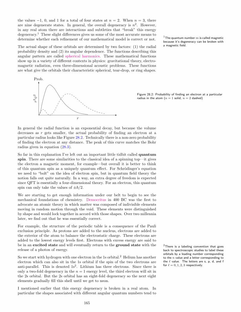
the values −1, 0, and 1 for a total of four states at n = 2. When n = 3, thereare nine degenerate states. In general, the overall degeneracy is n2. However,in any real atom there are interactions and subtleties that “break” this energydegeneracy.1 These slight differences gives us some of the most accurate means to

1The quantum number m is called magneticbecause it’s degeneracy can be broken witha magnetic field.

determine whether each refinement of our mathematical model is correct or not.

The actual shape of these orbitals are determined by two factors: (1) the radialprobability density and (2) its angular dependence. The functions describing thisangular pattern are called spherical harmonics. These mathematical functionsshow up in a variety of different contexts in physics: gravitational theory, electro-magnetic radiation, even three-dimensional acoustic problems. These functionsare what give the orbitals their characteristic spherical, tear-drop, or ring shapes.

r

Prob.

r2ψ

2 Figure 28.2: Probability of finding an electron at a particularradius in the atom (n = 1 solid, n = 2 dashed)

In general the radial function is an exponential decay, but because the volumedecreases as r gets smaller, the actual probability of finding an electron at aparticular radius looks like Figure 28.2. Technically there is a non-zero probabilityof finding the electron at any distance. The peak of this curve matches the Bohrradius given in equation (28.3).

So far in this explanation I’ve left out an important little tidbit called quantumspin. There are some similarities to the classical idea of a spinning top—it givesthe electron a magnetic moment, for example—but overall it is better to thinkof this quantum spin as a uniquely quantum effect. For Schrodinger’s equationwe need to “bolt” on the idea of electron spin, but in quantum field theory thenotion falls out quite naturally. In a way, an extra degree of freedom is expectedsince QFT is essentially a four-dimensional theory. For an electron, this quantumspin can only take the values of ±~/2.

We are starting to get enough information under our belt to begin to see themechanical foundations of chemistry. Democritus in 400 BC was the first toadvocate an atomic theory in which matter was composed of indivisible elementsmoving in random motion through the void. These elements were distinguishedby shape and would lock together in accord with those shapes. Over two millennialater, we find out that he was essentially correct.

For example, the structure of the periodic table is a consequence of the Pauliexclusion principle. As protons are added to the nucleus, electrons are added tothe exterior of the atom to balance the electrostatic charge. These electrons areadded to the lowest energy levels first. Electrons with excess energy are said tobe in an excited state and will eventually return to the ground state with therelease of a photon of energy.

So we start with hydrogen with one electron in the 1s orbital.2 Helium has another

2There is a labeling convention that goesback to spectroscopic studies to label theseorbitals by a leading number correspondingto the n value and a letter corresponding tothe ` value. The letters are s, p, d, and ffor ` = 0, 1, 2, 3 respectively.

electron which can also sit in the 1s orbital if the spin of the two electrons areanti-parallel. This is denoted 1s2. Lithium has three electrons. Since there isonly a two-fold degeneracy in the n = 1 energy level, the third electron will sit inthe 2s orbital. But the 2s orbital has an eight-fold degeneracy so the next eightelements gradually fill this shell until we get to neon.

I mentioned earlier that this energy degeneracy is broken in a real atom. Inparticular the shapes associated with different angular quantum numbers tend to

165

favor the more spherical shapes, or lower ` values. So, in general, the orbitals fillfrom s to p to d to f if possible given the value of the principle quantum numbern. Thus, the orbital configuration for boron is 1s22s22p1.

After neon, things get a little more tricky. This is because the energy level of the3s orbital is actually lower than the 2d orbital. In fact, the energy order of theorbitals is

1s 2s 2p 3s 3p 4s 3d 4p 5s 4d 5p 6s 4f 5d 6p 7s 5f 6d 7p 8s 5g 6f 7d 8p

Filling the electron shells according to this order will reproduce the period table(with a couple of exceptions).

Figure 28.3: The electron fields from twohydrogen atoms can overlap constructivelyor destructively (image credit here)

The covalent bond is also a uniquely quantum mechanical effect. Consider thehydrogen molecule H2. As the electron fields from the two atoms overlap, theymay either constructively or destructively interfere (see Figure 28.3). It happensthat the interference type is related to the quantum spin of each electron. If thetwo electron spins are aligned (parallel), the two waves constructively interfereand the overall energy of the system decreases. This reduction in energy is calledthe exchange interaction.

Figure 28.4: Energy levels for the twooverlap patterns in Figure 28.3 as the atomsapproach one another (image credit here)

There is a point of equilibrium in which the electrostatic repulsion of the twoelectrons is compensated by this exchange interaction (see Figure 28.4). At thispoint the wave function for the electron pair is largest between the two hydrogennuclei—we say the two are “sharing” the electrons. This constructive overlap isresponsible for every covalent bond in chemistry.

A secondary consequence of the covalent bond is that it induces an electric dipolemoment in the molecule by localizing the electrons between the nuclei. This effectis most pronounced when hydrogen is involved because it creates the maximumexposure of the positive nucleus. This is the source of the hydrogen bond whichis essentially electrostatic in nature. The hydrogen bond is responsible for many ofthe properties of water (including the fact that ice is less dense than cold water),the structure of proteins, and holds the DNA molecule together.

The exchange interaction is also responsible for magnets. You remember fromLecture 24 that every spinning charge acts like a magnet. So, every atom is alsomagnetic because of both the intrinsic and orbital spin of all its parts. However,in classical mechanics the alignment of these atoms is completely random withoutany long-range order. Part of the reason for this is that magnetic fields do nowork. This means that classical mechanics cannot explain the existence of barmagnets!

There are actually three forms of natural magnetism: ferromagnetism, param-agnetism, and diamagnetism. Ferromagnetism is the strongest type and isexhibited in the typical bar magnet. Paramagnetism is the type of magnetisminvolved in materials we would call “magnetic” in the sense that a natural magnetwill “stick” to the substance. This is due to an induced dipole magnetic momentwhich acts to attract the magnet to the material. Diamagnetism occurs in “non-magnetic” materials like aluminum or plastic. This effect is actually repulsive andis ultimately due to Lenz’s law (page ??) applied on the atomic scale.3

3This phenomena has been used to sta-bilize some interesting levitation experi-ments. See here to read about levitatinglive frogs. . .

But ferromagnetism has no classical analog. It is another manifestation of theexchange interaction which creates a lower energy state when the magnetic mo-ments of the atoms are parallel. In a way we have a “magnetic covalent bond”which forms and yields an alignment of the atomic magnetic moments to createa macroscopic dipole moment.

Actually, ferromagnetism is our first step into solid state physics.4 Classically we

4Solid state physics is a branch of con-densed matter physics, which includes thestudy of all phases of matter: gas, liq-uid, and solid. It also studies the electricand magnetic properties of matter includingmore exotic phenomena like superconductiv-ity. Nanotechnology (the manipulation ofmatter on an atomic scale) is also consid-ered a branch of condensed matter physics.

have already imagined a solid like set of balls connected by springs (cf. Lecture13). We now hope to see what happens when we apply quantum mechanics to acollection of atoms locked together in a solid.

166

Take another look at Figure 28.4. Notice how when the separation between thehydrogen atoms is large the electrons are both at −13.6 eV. As they approachone another this equality splits. If we add another atom to the system, the energylevels split again. Add a whole crystal of atoms and the energy levels form anenergy band of closely spaced levels. This allows the electrons to gain a smallamount of kinetic energy to move rather than being locked into one particularenergy level.

Each orbital from the original atoms creates an energy band (see here for aninteresting diagram). Frequently there are gaps between the bands—energy levelsinaccessible to the electrons. As the atoms collect into the crystal, the electrons fillthe lowest energy bands first. These bands are either completely full or completelyempty. Bands that are filled are called valence bands and those that are emptyare called conduction bands. It is possible that the bands overlap—if thatoccurs between the last valence band and the first conduction band, then theelectrons are free to move and we have a conductor. On the other hand, anenergy gap creates an insulator. See Figure 28.5.

Insulator

Egap

Filledvalenceband

Emptyconductionband

Conductor

E

Figure 28.5: Energy band description ofinsulators and conductors

But this description ignores the effect of temperature on the energy distributionof the electrons. At any temperature, there is a probability that any individualelectron will gain enough kinetic energy to overcome this energy gap. It can beshown that the density of electrons that do this is related to both temperatureand the energy gap by

ρ = (AT 3/2) exp(−Egap/2kT ) (28.5)

where A = 0.00805 mol/m3. The important factor is the exponential. Unlessthe energy gap is on the order of an electron volt, this temperature effect iscompletely negligible. For example, silicon has a band gap of 1.1 eV, so at 300kelvin (approximately room temperature), equation (28.5) implies an electrondensity of 3.28 × 10−8 moles of electrons per cubic meter. Though small, this isenough to allow a small amount of current to flow.

So even if the bands don’t overlap, there is a second way for a material toconduct electricity. Those materials with an energy gap around 1 eV are calledsemiconductors.

One of the reasons for the tremendous utility of semiconductors in electronics isthe ability to precisely control the electrical properties through doping. If wediffuse a small amount of phosphorous (typically via phosphine gas PH3) into puresilicon we introduce an extra energy level just below the conduction band filledwith extra electrons because phosphorous has five outer electrons but the latticestructure of silicon only supports four. This is called an n-type semiconductorbecause of the addition of negative charges.

We can do the opposite too by diffusing boron (typically via diborane gas B2H6)which introduces an empty energy level just above the valence band. This givesthe electrons trapped in the valence band a bit of room to move. If an electronjumps up to this extra energy level it leaves behind a “hole” in the valence band.A neighboring electron can jump into it leaving behind another hole. This holeacts exactly like a positively charged electron in that it moves in the oppositedirection as the electrons with the same speed and effective mass. Though anartifact of the gaps in the electron “gas” produced by introducing boron, it isconvenient to consider this hole as particle in its own right,5 so we call this a

5In fact, when Dirac was working out arelativistic version of Schrodinger’s equation(27.2), he predicted the existence of thepositron in the very same way.

p-type semiconductor.

But this is just the beginning. Now take p-type and n-type materials and putthem together. This is called a pn junction and is fundamental to any integratedcircuit. At the interface between the two materials, the free electrons in the n-typematerials jump over to holes in the p-type material.6 This creates a separation

6Notice that the p-type material has a netnegative charge and the n-type material hasa net positive charge—the naming conven-tion gets a bit confusing at this point.

of charges which creates an internal voltage difference across the interface. Thisvoltage difference opposes the flow of electrons and an equilibrium state is reached

167

as in Figure 28.6. This internal voltage is dependent upon the nature of the twomaterials making the junction.

p n−−−

+

+

+

E

V

Figure 28.6: The equilibrium state of apn-junction and the internal potential thatmust be overcome for current to flow freely.

Suppose we connect the positive terminal of a battery to the p side of the junctionand the negative terminal to the n side. What happens is that the battery siphonsoff the electrons that collected in the p-type material (if the battery voltage islarge enough to overcome the intrinsic voltage of the junction which is about0.6 eV for a silicon-based diode). This disturbs the equilibrium and allows moreelectrons to flow from the n-type material and current flows freely.

Hook the battery up the other way and the current is blocked. This is becausethe battery voltage must exceed the internal voltage for current to flow. But asthe current flows, it contributes to this internal voltage (like a capacitor) and itbuilds up until it is equal to the battery voltage.

So the pn junction acts like a one-way street for current. When we treat this pnjunction as an electronic component it is called a diode.7

7This terminology actually comes from thedays of vacuum tubes—which are still usedin some industrial applications (see here).

As current flows in a diode, each electron jumps from the conduction band inthe n-type material to the valence band in the p-type material. When the diodeis forward biased these levels are separated by an amount equal to the internalvoltage at equilibrium. This means that each electron drops in energy just likewhen the electron in an exited atom falls to its ground state. However, not everypn junction will emit photons: the change in momentum has to be lined up too.8

8This is true of the atom also: transitionsbetween any two states is not possible ingeneral. But typically the angular mo-mentum states are degenerate so there isalways a way to get from one energy levelto another.

If so, the band gap is said to be “direct” and the energy drop is released asa photon (silicon based diodes have indirect band gaps). If the drop creates aphoton with a frequency in the visible range, we have a light-emitting diode,or LED. Run this process in reverse and you have a solar cell.

We can’t leave this subject without talking about the transistor which is essen-tially two diodes placed back-to-back. A pnp transistor has an internal voltagepattern that looks like a potential barrier to current. By controlling the dopinglevels we can control which side has higher and lower potential. The higherpotential end is called the collector and the lower potential the emitter.

The central n region is called the base of the transistor. By applying a voltage tothe base we can control the height of the potential barrier within the transistor.When the voltage on the base pulls the potential barrier down, current flowsfrom the collector to the emitter (these names are a consequence of the fact thatelectrons move in the opposite direction because they have negative charge).

So a transistor acts as a miniature electronic switch which makes it ideal forcomputers. It also can be used as an amplifier since the base voltage—whichuses a small amount of current—can control a large flow of current between thecollector and emitter. Every integrated circuit is a combination of seeminglyendless combinations of these diodes, transistors, and more.

Next week we continue our studies down in scale to talk about the nucleus ofthe atom. Each nucleus is composed of positively charged protons and particleswithout electric charge called neutrons. We will discuss how each nucleus is intension balancing the electrostatic repulsion of its protons and the strong nuclearforce. For larger nuclei this balance becomes unstable and natural radioactivityis a result. This tension also offers a way of unleashing the power of the strongnuclear force in controlled (and uncontrolled) ways.

168

Lecture 29

Nuclear EnergyRead sections 31.1–31.7 and 32.1–32.5

Just a casual observation of the periodic table will uncover a problem: the atomicmasses do not increase in step with the atomic number. One would expect thathelium would be twice as massive as hydrogen, lithium three times, etc. But notso—its 1, 4, 7, 9, 11ish, 12, 14, 16, 19 for the first nine elements. And what is upwith boron at 10.8?

Initially it was supposed that, for example, nitrogen had 14 protons in its nucleus(which accounts for the mass) that had somehow swallowed seven of its electrons(which accounts for the charge). However, no arrangement of 21 particles cancorrectly account for its quantum spin.

In 1920, Rutherford offered the idea of a third subatomic particle in the nucleus.Without charge and with mass similar to the proton, this neutron was laterdiscovered in 1932. The atomic number of the atom describes the number ofprotons and drives the chemistry of the element (by attracting the same numberof electrons), and the remaining mass is provided by the neutrons.

We can even explain our “11ish” mass for boron as the average mass of severalisotopes, or atoms with the same number of protons but a different number ofneutrons. Isotopes have different masses but are indistinguishable chemically. Inthe case of boron we have two stable isotopes: boron-10 and boron-11 with fiveand six neutrons respectively.1 The relative abundance of the two are 20% and

1These are usually denoted 105B and 11

5B butit is so much easier to write, type and sayboron-10 and boron-11 that I will almostexclusively do so.

80% which yields an average mass of 10.8.

The neutrons stabilize the nucleus by pitting the strong nuclear force against theelectrostatic repulsion of the protons. Although protons do participate in thestrong force, their repulsion is too great to allow them to bind together: heliummust have at least one neutron.

On the other hand, the neutron needs the proton too. In isolation, the neutron isunstable and decays into a proton and an electron with a mean lifetime of about15 minutes. But in the nucleus the neutron can be stable.2

2It may look like this validates the idea ofthe neutron as some sort of bound statebetween the proton and the electron. Butthe story is a more complicated than that.We will pick this up again in Lecture 30.

However, when the nucleus becomes too large these balancing acts begin to fail.The heaviest stable isotope is lead-208. Nuclei heavier than this are radioactivemeaning they decompose and release nuclear radiation.

A common way for nuclei to shed excess size is by alpha decay. One of thefirst forms of radiation studied, the α-particle was later determined to be a pairof protons and neutrons (an helium nucleus).3 This alpha radiation is easily

3This is the source of helium on our planet.Every helium balloon you see is filled withthe byproduct of billions of years of radioac-tivity.

shielded by a piece of paper or even just a few centimeters of air.4 This mode of4Smoke detectors work by using an alpharadiation source. The alarm is designed tosound whenever the transmission of the α-particles is blocked (presumably by smoke).

decay is said to be transmutation since it actually changes the chemical element

169

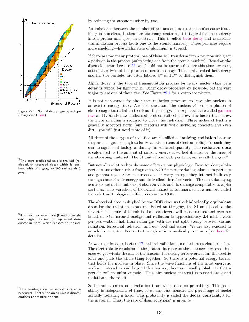
by reducing the atomic number by two.

An imbalance between the number of protons and neutrons can also cause insta-bility in a nucleus. If there are too many neutrons, it is typical for one to decayinto a proton and eject an electron. This is called beta decay and is anothertransmutation process (adds one to the atomic number). These particles requiremore shielding—five millimeters of aluminum is typical.

If there are too many protons, one of them will transform into a neutron and ejecta positron in the process (subtracting one from the atomic number). Based on thediscussion from Lecture 27, we should not be surprised to see this time-reversed,anti-matter twin of the process of neutron decay. This is also called beta decayand the two particles are often labeled β− and β+ to distinguish them.

Alpha decay is the typical transmutation process for heavy nuclei while betadecay is typical for light nuclei. Other decay processes are possible, but the vastmajority are one of these two. See Figure 29.1 for a complete picture.

Figure 29.1: Normal decay type by isotope(image credit here)

It is not uncommon for these transmutation processes to leave the nucleus inan excited energy state. And like the atom, the nucleus will emit a photon ofelectromagnetic radiation to release this energy. These photons are called gammarays and typically have millions of electron-volts of energy. The higher the energy,the more shielding is required to block this radiation. Three inches of lead is agenerally accepted norm (any material will work including concrete and evendirt—you will just need more of it).

All three of these types of radiation are classified as ionizing radiation becausethey are energetic enough to ionize an atom (tens of electron-volts). As such theycan do significant biological damage in sufficient quantity. The radiation doseis calculated as the amount of ionizing energy absorbed divided by the mass ofthe absorbing material. The SI unit of one joule per kilogram is called a gray.5

5The more traditional unit is the rad (ra-dioactivity absorbed dose) which is one-hundredth of a gray, so 100 rad equals 1gray.

But not all radiation has the same effect on our physiology. Dose for dose, alphaparticles and other nuclear fragments do 20 times more damage than beta particlesand gamma rays. Since neutrons do not carry charge, they interact indirectlythrough sheer kinetic energy and their effect therefore varies. The most damagingneutrons are in the millions of electron-volts and do damage comparable to alphaparticles. This variation of biological impact is summarized in a number calledthe relative biological effectiveness, or RBE.

The absorbed dose multiplied by the RBE gives us the biologically equivalentdose for the radiation exposure. Based on the gray, the SI unit is called thesievert.6 The rule of thumb is that one sievert will cause nausea and over six

6It is much more common (though stronglydiscouraged) to see this equivalent dosequoted in “rem” which is based on the rad.

is lethal. Our natural background radiation is approximately 2.4 millisievertsper year—about half from radon gas with the rest split evenly between cosmicradiation, terrestrial radiation, and our food and water. We are also exposed toan additional 0.4 millisieverts through various medical procedures (see here fordetails).

As was mentioned in Lecture 27, natural radiation is a quantum mechanical effect.The electrostatic repulsion of the protons increase as the distances decrease, butonce we get within the size of the nucleus, the strong force overwhelms the electricforce and pulls the whole thing together. So there is a potential energy barrierthat holds the nucleus in place. Since the wave functions of the most energeticnuclear material extend beyond this barrier, there is a small probability that aparticle will manifest outside. Thus the nuclear material is pushed away andradiation is the result.

So the actual emission of radiation is an event based on probability. This prob-ability is independent of time, so at any one moment the percentage of nucleiactually radiating is fixed. This probability is called the decay constant, λ forthe material. Thus, the rate of disintegrations7 is given by

7One disintegration per second is called abecquerel. Another common unit is disinte-grations per minute or bpm.

170

∆N

∆t= −λN (29.1)

This quantity is called the activity of the material. From this it follows that theamount of substance left after a particular time period is

N = N0 exp(−λt) (29.2)

It can be shown from this equation that the mean life-time τ of a particle is equalto 1/λ. The half-life of the material is the amount of time it takes for half of theinitial substance to disintegrate and we see that

T1/2 =ln 2

λ= τ ln 2 (29.3)

The half-life of carbon-14 is 5730 years, so its decay constant λ is 3.84× 10−12.

Radiocarbon dating works by comparing the amount of carbon-14 to carbon-12in a substance. Natural carbon-14 is created by cosmic rays interacting withthe nitrogen gas in the atmosphere. A dynamic equilibrium exists between theradioactive decay and this cosmic generation which fixes the amount of carbon-14in the atmosphere. As such, living creatures breathe and consume both carbon-12and carbon-14 in a fixed ratio.

When a plant or animal dies, the level of carbon-14 becomes depleted over time.By measuring the radioactive activity in a specimen we can use equation (29.1)to determine the amount of carbon-14 currently present. Measuring the amountof carbon-12 gives us a way to estimate the original amount of carbon-14. Usingequation (29.2) we can get to an approximate time of death:

t =1

λln

(N0

N

)(29.4)

where N is the current amount of carbon-14 inferred from the measured activity ofthe sample and N0 is the original amount of carbon-14 inferred from the amountof carbon-12 in the sample.

So far in this lecture we have focused on natural forms of radioactivity andtransmutation. We now turn to consider how we can use this information toinduce various nuclear interactions. The most important item to consider in thiscontext is the nuclear binding energy curve in Figure 29.2. This curve representsthe net energy needed to break apart stable nuclei into their component parts.

Figure 29.2: Nuclear binding energy curve (image credit here)

Note that this is not the energy required to overcome the strong nuclear force andbreak apart the nucleus (the “activation energy” to use the chemical term). Ifthis barrier energy is overcome, electrostatic repulsion will create kinetic energypushing apart the protons to infinity. The binding energy is the attractive energy

171

from the strong force minus the repulsive energy from the electrostatic force andrepresents the average energy level of the nuclear material in the nucleus. Iron-56is the most stable of all nuclei with a binding energy of 8.8 MeV per nucleon.8

8A nucleon is a catch-all term to describeboth protons and neutrons.

The high binding energy for helium-4 (at 7.1 MeV per nucleon) explains whyheavy radioactive nuclei tend to decay using alpha particles rather than tritiumor lithium-6 or some other combination of protons and neutrons.

Using Figure 29.2 we can calculate the energy involved in various nuclear re-actions. Nuclear fusion occurs when we combine nuclei to generate a largercomposite (we called this an inelastic collision in Lecture 8). The fact that thebinding curve goes up initially indicates that fusion in exothermic: more energyis released when the end products combine than required to break apart thebeginning nuclei. This is the kind of nuclear process that powers the sun.

The binding curve increases up to iron-56 after which fusion is endothermic: itrequires a net expenditure of energy to create these nuclei. But this also impliesthat the reverse process, nuclear fission, can be used as an energy source. Thisis the kind of nuclear process used in nuclear power plants today.

In either nuclear fusion or fission, we can use the binding energy curve to calculatethe net energy requirements for the process. However, there is an easier wayusing the so-called mass defect. This is a statement of the fact that the masson the two sides of a nuclear reaction do not balance. The difference is simplya consequence of E = mc2 and the binding energy involved. Every difference ofone atomic mass unit corresponds to 931.5 MeV of energy. When one takes intoaccount the “mass” of the binding energy, the equations balance.

For example, let’s calculate the binding energy of the helium atom. We have twoprotons, two neutrons, and two electrons. The atomic masses of these particlesare in Table 29.1. The total of all six particles is 4.032 980 atomic mass unitswhile the helium atom is only 4.002 602. This is mass deficit of 0.030 378 atomicmass units, so the helium-4 atom has a binding energy of 28.3 MeV.

Electron 0.000 549 amu

Proton 1.007 276 amu

Neutron 1.008 665 amu

Table 29.1: Atomic masses of the threeparticles that make up the atom

The atomic masses of the isotopes are readily available (here for example, or lookup the wikipedia article “isotopes of helium”, etc.). In order to figure out theenergy released in a particular nuclear reaction, we simply calculate the differencein mass and convert it to energy via E = mc2.

The first man-made fission reaction involved bombarding uranium-235 with neu-trons. One possible reaction (of many) is the following:

23592U + 1

0n→ 14456Ba + 89

36Kr + 310n

The atomic masses for uranium-235, barium-144, and krypton-89 are 235.043 930,143.922 953, and 88.917 636 respectively. The total mass on the left-hand side ofthis reaction is 236.052 590 and the right-hand side is 235.866 580, which leaves amass defect of 0.186 010 atomic mass units. This means that each fission reactiongenerates 173 MeV of energy.

On average, the fission of uranium-235 yields 215 MeV of energy with 2.4 neutronsas a byproduct. These extra neutrons are typically too energetic to initiate asecondary reaction unless the concentration of uranium-235 (relative to uranium-238) is in excess of 90%—which is called weapons-grade uranium.9 However, a

9Plutonium-239 will also support a chain re-action and can be generated by bombardinguranium-238 with neutrons.

moderator (like graphite) can be used to slow the neutrons down in order tocreate a controlled chain-reaction. Nuclear reactors work this way with a smallerconcentration around 20% and harness the energy through a high-efficiency steamengine. The amount of energy generated by the fission of one kilogram of uranium-235 could easily provide the energy needs of one person for a lifetime.

The problem with nuclear fission as an energy source is the radioactive wasteproducts. On the other end of the scale we have fusion which powers the sun.Fusion packs more power per kilogram of fuel which can be seen by comparingthe slopes on the left and right of the binding energy curve in Figure 29.2. One

172

of the most promising nuclear reactions for fusion on earth is the combinationof deuterium (hydrogen-2, atomic mass of 2.014 102) and tritium (hydrogen-3,atomic mass of 3.016 049):

21H + 3

1H→ 42He + 1

0n

The mass on the left-hand side of this reaction is 5.030 151 and the right-handside is 5.011 267, for a mass deficit of 0.018 884 atomic mass units. This reactionproduces 17.6 MeV of energy, or 3.52 MeV per nucleon. The fission of uranium-235 was about 0.915 MeV per nucleon, so pound-for-pound this reaction is almostfour times more powerful—with helium as the main waste product.

There are two problems with this approach. The first is the fuel: deuteriumis relatively plentiful and could be extracted from sea water, but tritium hasa half-life of about 12 years (decay product is helium-3). So there is not mucharound—it would have to be generated (by bombarding lithium-6 with neutrons).This would take some work, but is possible.

The real problem is that no one has yet been able to control these fuels withenough precision to consistently overcome the “activation barrier” to release thefusion energy. This high level of energy requires the hydrogen isotopes to bein a plasma with a temperature over 450 million kelvin. These temperatureshave been reached—the problem is constricting this plasma to create some sortof magnetic confinement fusion. Plasma is electromagnetically active whichmakes it extremely unstable and unwieldy. The tokamak uses a toroidal (donut)shaped magnetic field to perform the necessary confinement. Several experimentaltokamaks have been constructed with some success and research is ongoing inorder to produce a workable structure.

Another approach to the problem is called inertial confinement fusion. Essen-tially the idea is to fire a high-energy laser or electron beam at a small pellet ofthe deuterium/tritium fuel. The beam burns off the outer layer explosively whichdrives an implosion of the inner layer. If a critical density and temperature canbe reached the fusion reaction will take place—just like a tiny atomic bomb.

Next week we finish off the course by investigating the very edge of what is knownin physics. The decay of the neutron is our stepping off point to talk about thestrong and weak nuclear interactions. We will find that protons and neutronsare made of quarks and we will discover we have overlooked the neutrino in ourprevious discussions. Quarks will help us make sense out of the “particle zoo” inhigh energy physics.

This is the “standard model” of elementary particles and our two nuclear interac-tions involve the exchange of new physical properties in the context of quantumfield theory. If we have time, we may even be able to talk about why people thinkthere is something beyond the standard model and whether string theory is thatfinal answer.

173

174

Lecture 30

High Energy PhysicsRead section 32.6–32.7 and review Lecture 27

Our humble neutron, which appeared as an add-on to the structure of the atom,turns out to play a central role in both the creation of nuclear fuel and theunleashing of nuclear energy. We will start this final lecture addressing one looseend from the previous one: neutron decay.

With regard to neutron decay, I left out an important fact from Lecture 29. Whenthe neutron decays three particles are produced not two. The extra particle iscalled a neutrino because it has no electric charge and is nearly massless.1

1Originally, the neutrino was assumed tobe massless. The phenomena of neutrinooscillation measured from the sun in 1998proves that the neutrino must have somemass. The current upper bound is 0.3 eV, orabout 1500 times lighter than the electron.

We now seek an explanation in terms of quantum field theory for the decay ofthe neutron. We can do this by considering some key Feynman diagrams. Wepostulate the existence of a new boson to mediate the interaction that controls thisdecay. The reason for this is that each vertex in a Feynman diagram always formsa triad with two fermion lines and one boson. We cannot have a fermion decayingdirectly into other fermions. Since this is called the weak nuclear interaction, wecall this new particle the weak boson (see Figure 30.1).

n

p+ ν e−

W−

Figure 30.1: Feynman diagram for neutrondecay. The weak boson creates valid ver-texes for the interaction.

We know a few of things about this boson. First, it is short-range which meansit is massive—about 80 GeV/c2. It can be shown that equation (27.8) yields thepotential formula

V ∝ exp(−r/a)

r(30.1)

where a = ~/mc represents the range of this potential. In QED the range isinfinite because the mass of the photon is zero. Based on the mass of the W -boson, the range of its influence is on the order of 10−17 meters. Second, itdecays with a very short time-frame—about 10−25 seconds which is a consequenceof its large mass. In this case, the W -boson decays into an electron and an anti-neutrino. Finally, it is charged since it converts a neutral object (the neutron)into a charged one (the proton). This means it has an anti-particle twin with theopposite charge.

If Figure 30.1 were a diagram from QED, we would interpret the decay of theweak boson as a matter-antimatter creation event. This is why the neutrino islabeled as its anti-particle. But the new characteristic of this diagram is that itpairs different particles together: the neutron with the proton and the electronwith the neutrino. There is more to this story, but we first need to develop someideas on the strong nuclear interaction to pull it all together.

The fact that the neutron can decay seems to imply that there is still somesubstructure to be found. But we know from Lecture 27 that the creation ofmatter from pure energy cannot be ruled out. However, there is more directevidence of substructure: the neutron has a magnetic moment.

175

A magnetic moment is generated by a rotating charge (see Lecture 24). It ispossible for an object with a net charge of zero to have a magnetic moment if thecharge is distributed across the object (like a dipole). This seems to imply thatthere are little charged parts tied together to form the neutron. This is, in fact,the case—they are called quarks.2

2If this seemingly endless substructureseems silly to you, you are not alone. Whenfirst proposed in the late 1960s, physicistswere reluctant to accept the quark theory.But when predicted particles were found inthe following decade (1974 to be precise),the theory carried the day.

The theory works if we assume the neutron is composed of three quarks: one“up” and two “down”. Don’t put too much thinking into the names: they areintended to merely distinguish the two as opposites.3 These quarks have a charge

3This is a common theme in particlephysics: an appalling lack of imagination innaming things. We’ve already seen this inthe “strong” and “weak” nuclear forces.

of +2/3 and −1/3 respectively. If we combine two “up” quarks and one “down”quark we get the proton. And like the way electromagnetism is mediated bythe exchange of photons, the strong interaction holds these triplets together byexchanging bosons called gluons (seriously. . . I’m not making this up).

The force that hold the nucleus together is actually the residual force left over fromthis strong quark interaction. Much like the way a magnet sticks to a refrigeratoror a balloon sticks to the wall via static electricity, the fields from the boundquarks interact to hold the composite protons and neutrons together.

The Feynman diagrams for the exchange of gluons look just like those in QED,but to explain the three-way nature of the strong interaction requires some work:we need a three-valued “charge”. This three-valued charge is called colour. Ofcourse, the quarks are not actually red or green or blue, but there is some logic tothis name. The basic rule of thumb is that quarks always combine to be colour-lessor to create “white”.

So the opposite of the red quark colour is green and blue together, and so on. Youcan imagine that the mathematics required to explain this is a bit complicated(this is why the SU(3) group is associated with colour). Figure 30.2 showsa schematic of what is happening. Remember, in quantum field theory youshould imagine that all of these interactions are occurring simultaneously andcontinuously.

Figure 30.2: How the exchange of colour holds the proton andneutron together.

g

r b

r −→g←−

t = 0

r

g b

r−→b←−

t = 1

b

g rg−→ r←−

t = 2

Qb Qr

Qr Qb

Grb

Figure 30.3: A fundamental diagram forthe strong interaction showing the colourexchange between quarks.

Let’s look in a little more detail at the Feynman diagram for a single colourexchange. In Figure 30.3 the Q represents a quark of any kind and G is the gluonmediating the colour exchange. In this diagram, blue is on the left and red is onthe right. The quark on the right emits the gluon which exchanges these colors.It takes red away and brings blue. But since the blue travels backward in time,we say the gluon is carrying red and anti-blue.

The idea of “anti-color” brings the last piece of the puzzle into play: anti-quarks.With this same construct we can bind a quark and an anti-quark together. Inthis case, the anti-quark actually carries anti-colour, so they can combine in acolour-neutral way by being red and anti-red, for example.

These two ways of combining quarks explain the so-called particle zoo. In thedecades before the theory of quarks was developed, many high energy collisionsexperiment were performed. Frequently new particles were formed in the collisionof electrons or protons. Over time, this continual discovery of new particles stirredup quite a bit of discomfort among physicists. Around 1930, it seemed that theworld could be explained with only three fundamental particles—now there wereover 70 “fundamental” particles. Clearly something needed some explaining!

176

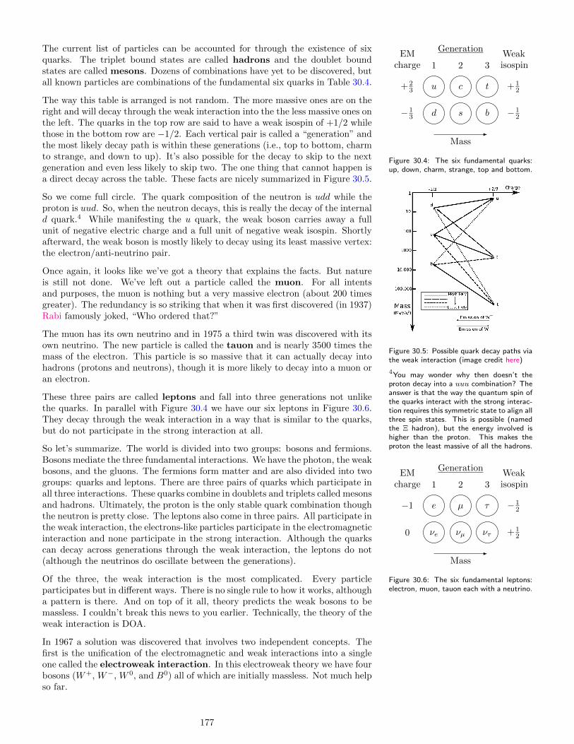
The current list of particles can be accounted for through the existence of sixquarks. The triplet bound states are called hadrons and the doublet boundstates are called mesons. Dozens of combinations have yet to be discovered, butall known particles are combinations of the fundamental six quarks in Table 30.4.

EMcharge

+ 23

− 13

1

u

d

Generation

2

c

s

3

t

b

Weakisospin

+ 12

− 12

Mass

Figure 30.4: The six fundamental quarks:up, down, charm, strange, top and bottom.

The way this table is arranged is not random. The more massive ones are on theright and will decay through the weak interaction into the the less massive ones onthe left. The quarks in the top row are said to have a weak isospin of +1/2 whilethose in the bottom row are −1/2. Each vertical pair is called a “generation” andthe most likely decay path is within these generations (i.e., top to bottom, charmto strange, and down to up). It’s also possible for the decay to skip to the nextgeneration and even less likely to skip two. The one thing that cannot happen isa direct decay across the table. These facts are nicely summarized in Figure 30.5.

Figure 30.5: Possible quark decay paths viathe weak interaction (image credit here)

So we come full circle. The quark composition of the neutron is udd while theproton is uud. So, when the neutron decays, this is really the decay of the internald quark.4 While manifesting the u quark, the weak boson carries away a full

4You may wonder why then doesn’t theproton decay into a uuu combination? Theanswer is that the way the quantum spin ofthe quarks interact with the strong interac-tion requires this symmetric state to align allthree spin states. This is possible (namedthe Ξ hadron), but the energy involved ishigher than the proton. This makes theproton the least massive of all the hadrons.

unit of negative electric charge and a full unit of negative weak isospin. Shortlyafterward, the weak boson is mostly likely to decay using its least massive vertex:the electron/anti-neutrino pair.

Once again, it looks like we’ve got a theory that explains the facts. But natureis still not done. We’ve left out a particle called the muon. For all intentsand purposes, the muon is nothing but a very massive electron (about 200 timesgreater). The redundancy is so striking that when it was first discovered (in 1937)Rabi famously joked, “Who ordered that?”

The muon has its own neutrino and in 1975 a third twin was discovered with itsown neutrino. The new particle is called the tauon and is nearly 3500 times themass of the electron. This particle is so massive that it can actually decay intohadrons (protons and neutrons), though it is more likely to decay into a muon oran electron.

These three pairs are called leptons and fall into three generations not unlikethe quarks. In parallel with Figure 30.4 we have our six leptons in Figure 30.6.They decay through the weak interaction in a way that is similar to the quarks,but do not participate in the strong interaction at all.

EMcharge

−1

0

1

e

νe

Generation

2

µ

νµ

3

τ

ντ

Weakisospin

− 12

+ 12

Mass

Figure 30.6: The six fundamental leptons:electron, muon, tauon each with a neutrino.

So let’s summarize. The world is divided into two groups: bosons and fermions.Bosons mediate the three fundamental interactions. We have the photon, the weakbosons, and the gluons. The fermions form matter and are also divided into twogroups: quarks and leptons. There are three pairs of quarks which participate inall three interactions. These quarks combine in doublets and triplets called mesonsand hadrons. Ultimately, the proton is the only stable quark combination thoughthe neutron is pretty close. The leptons also come in three pairs. All participate inthe weak interaction, the electrons-like particles participate in the electromagneticinteraction and none participate in the strong interaction. Although the quarkscan decay across generations through the weak interaction, the leptons do not(although the neutrinos do oscillate between the generations).

Of the three, the weak interaction is the most complicated. Every particleparticipates but in different ways. There is no single rule to how it works, althougha pattern is there. And on top of it all, theory predicts the weak bosons to bemassless. I couldn’t break this news to you earlier. Technically, the theory of theweak interaction is DOA.

In 1967 a solution was discovered that involves two independent concepts. Thefirst is the unification of the electromagnetic and weak interactions into a singleone called the electroweak interaction. In this electroweak theory we have fourbosons (W+, W−, W 0, and B0) all of which are initially massless. Not much helpso far.

177

The second concept is called the Higgs mechanism which postulates the exis-tence of yet another entity called the Higgs field. The idea runs like this. At veryhigh temperatures the four electroweak boson and the Higgs field exist in a kindof equilibrium. But when the energy level of the temperature drops below themass of the weak bosons (kT = 80 GeV/c2 or T = 1015 kelvin), this equilibriumgo unstable and the quantum symmetries “break”5 and the Higgs field “mixes”

5This spontaneous symmetry breaking canbe understood by example: consider whathappens when a liquid freezes. As a liquidthe molecules are oriented in all directionswith no preference. But as the temperaturedrops, the molecules line up in a crystalstructure and breaks the symmetry. Now, itis possible for a liquid to go into an unstablesupercooled state. Some sort of asymmetrictrigger is required to break the symmetry.But the point is that the preferred directionis not inherent in the physical laws governingthe material. When the system moves toan unstable region (through lower tempera-ture) the smallest trigger will lock the wholesystem in place.

with the electroweak bosons.

This mixing causes the W+ and W− bosons to acquire mass and the B0 bosonbecomes the photon. We also have two other residual particles: the Z boson whichis what is left of the original W 0 boson and the Higgs boson which is what is leftof the original Higgs field. The Z boson has been observed (about 92 GeV/c2)and acts like a heavy photon (it doesn’t carry electric charge or weak isospin,so it doesn’t change the nature of the particle). The Higgs boson has yet to beobserved—this is one of the main objectives of the Large Hadron Collider.6

6There may be ways to break the elec-troweak symmetry without the Higgs boson.See here for details.

This approach may look convoluted and unmotivated. It is inspired by theBCS theory of superconductivity. Electrons pair up in a superconductor andact like bosons which gives the superconductor its non-classical behavior. Asuperconductor is a system involving massive “bosons” about which we know quitea bit. So it makes sense that this theory might act as a template to understandthe weak boson.

Table 30.1: The observed masses of the weak bosons matchwell with those predicted by the electroweak theory (takenfrom here)

Boson Measured Predicted

W 80.398 ± 0.025 80.390 ± 0.018

Z 91.1876 ± 0.0021 91.1874 ± 0.0021

Nonetheless, I don’t think anyone would call the theory “pretty”. But it doeswork, and from a bottom-line perspective that’s enough (see Table 30.1). Thephysicists working this out in the decades prior to 1980 or so seem to have expectedthis complexity to disappear in some overarching “theory of everything”. As such,the combination of the electroweak theory and the strong interaction now goesby the unimpressive name of the Standard Model of particle physics. Figure30.7 shows our new periodic chart for elementary particles.

Electron

e0.511

Legend

Symbol

Name

Mass

Electron

e0.511

Neutrino

νe> 0

Quark

d4.8

Quark

u2.4

Muon

µ106

Neutrino

νµ> 0

Quark

s100

Quark

c1300

Tauon

τ1800

Neutrino

ντ> 0

Quark

b4200

Quark

t170000

Spin 1/2 particles(Fermions)

Photon

γ0

−1

0

− 13

+ 23

Gluon

g0

0

0

g

g

Weak

W∼ 80000

− 12

+ 12

− 12

+ 12

Leptons

Quarks

Spin 1 particles(Bosons)

Figure 30.7: The elementary particles according to the Standard Model. (Inspired by a similar chart in Feynman’s book QED: The Strange Theoryof Light and Matter.)

The Standard Model is an extremely successful theory: one that has yet to makea prediction that is incompatible with experiment. Yet physicists continue to talkabout the “next” theory. Why?

178

The short answer is that the model appears incomplete. Clearly we need toincorporate gravity yet it is not clear how this can be done. The Higgs particlehas yet to be found—what if it’s not there? Also, there are things that happenin nature that the original model does not anticipate like parity violation7 and

7This parity violation implies that naturemakes a slight distinction between matterand anti-matter. This could explain theapparent imbalance in the universe betweenthe two.

neutrino oscillation. These features can be “bolted” on to the model to matchexperiment by tweaking and fine tuning the formulas, but a complete theoryreally ought to predict these features naturally. And then there are other thingsthat you would expect the theory to explain that it does not. For example, isthere a pattern to the particle masses?8 How did the weak symmetry break and

8Note that the periodic table does offer anexplanation for each atomic mass.

why did it fall out in this particular way? Why are there three generations ofparticles—are there more?9 Finally there are suspicious coincidences: Why three

9Neutrino oscillation provides evidence thatthere are only three kinds of neutrinos, butit does not explain why.

generations of both quarks and leptons? Why is the charge of the electron andproton exactly the same?

It’s these last two questions that have motivated physicists to postulate some sortof “supersymmetry” between the leptons and fermions which unifies the strongand electroweak interactions. Inspired by the success of the electroweak theoryand even the memory of the unification of the electric and magnetic forces thesemodels are called grand unified theories (GUT). None work. The main problemthat they all have is that they predict the decay of the proton: just as the weakinteraction decays the quarks and leptons down the three generations into lessmassive particles, so should this “supersymmetry” decay the proton down intoelectrons and neutrinos. No one has ever witnessed the decay of the proton—thecurrent lower bound on the half-life of the proton is 1033 years and growing everyday.

And then there is gravity. . . . This is where string theory enters the picture.But before I explain these speculations let’s be very clear: we are deep in thewilderness here and the forest is very dark.10 We are still waiting to see if we

10It is a bit of a pet peeve of mine thatthe hypothetical fringe of physics is oftenrepresented as fact. For example, thereis no evidence for a “graviton”—it’s justa guess that a quantum theory of gravitymight have them. The unification of forcesgoing back to the Big Bang is another:the “inflation phase” of the early universeis a way of solving the horizon problem,but this presupposes unification rather thanproviding evidence for it.

understand the electroweak unification correctly and we know that unifying thestrong interaction has fundamental problems. The “Hail Mary” approach of stringtheory is a long shot indeed.

Nonetheless, the approach has prestigious roots: Einstein spent the last decadesof his life working on it. He was inspired by the quirky observation that if oneexpands general relativity to five dimensions, Maxwell’s equations pop out. Thereare problems, of course. There are no fermions, there are unobserved extra bosons,and it doesn’t say anything about the strong and weak interactions. Einsteinappears to have hoped to see an explanation for quantum mechanics come out ofthe theory, but it never did work.

But the “extra-dimension” seed had been planted and fifty years later stringtheory blossomed. Many theoretical facts about quantum strings vibrating in10 dimensions were uncovered which yield supersymmetry with a new boson tomediate the force of gravity. The mathematics is obscure but in the end thereappears to be five different options for a viable string theory. In the mid-1990’sa single 11-dimensional version based on vibrating membranes was developedwhich incorporates the five as special cases. Currently much speculation (andcontroversy) is focused on this “M-theory” as the final unification of fundamentalphysics.

That’s it. In Lecture 1 we began without even knowing how to define physics.Now we are at the very edge of what we know (and a bit beyond). It’s been quitea ride and I hope you learned a bit in the process. Study hard and fare well.

179

Index

aberration, 118absolute zero, 88acceleration, 16action, 42activity, 171adiabatic, 100alternating current, 144ampere, 137Ampere’s law, 141amplitude, 69angular displacement, 50angular frequency, 71angular momentum, 60anti-nodes, 111aphelion, 63arc-length, 49Archimedes’ principle, 82atomic hypothesis, 93atomic mass units, 94attenuation, 124Atwood machine, 29Avagadro’s number, 93average velocity, 15

back EMF, 145Balmer lines, 163bandwidth, 148base, 168beat frequency, 113beats, 112Bernoulli’s equation, 84binomial theorem, 8biologically equivalent dose, 170birefringence, 124black hole, 68, 154blackbody, 97Bohr model, 129Bohr radius, 164Boltzmann constant, 94bosons, 130, 161Brownian motion, 93bulk modulus, 76buoyant force, 82butterfly effect, 85

capacitance, 135capacitor, 133Carnot cycle, 101Celsius scale, 88center of gravity, 58

center of mass, 47center of mass frame, 47central force, 35centrifugal force, 31, 52centripetal force, 34coefficient of friction, 24coefficient of restitution, 45coefficient of thermal expansion, 88coherence, 124collector, 168colour, 176completely inelastic collision, 45conduction bands, 167conductivity, 138conductors, 131conservation of energy, 39constitutive equation, 24constraint forces, 23constructive interference, 109continuity equation, 83continuum mechanics, 77Coriolis force, 52Coulomb’s law, 131critical angle, 117critically damped, 73cross product, 12curl, 134current, 44, 137

dark matter, 36de Broglie wavelength, 157decay constant, 170decibels, 108degenerate states, 164degrees of freedom, 49delta-v, 46derivative, 7destructive interference, 109desynchronization, 151deterministic chaos, 85diamagnetism, 142, 166dielectric, 135dielectric constant, 135diffraction, 122diffraction grating, 123diffusion, 96diffusion constant, 96diode, 168diopters, 118dipole moment, 132

180

dispersion, 107displacement current, 149divergence, 134doping, 167dot product, 12double slit, 121dynamic balancing, 61dynamic equilibrium, 22dynamic pressure, 84

eccentricity, 64edge effects, 133effective potential, 64efficiency, 23, 38, 101elastic collision, 45electric constant, 133electric field, 132electric generator, 144electrical interference, 145electromagnet, 142electroweak interaction, 177elevation head, 84ELI the ICE man, 147EMF, 137emissivity, 89emitter, 168energy, 38energy band, 167entropy, 102equilibrium, 21equipartition principle, 96equipotential, 134equivalence principle, 31, 154ergosphere, 80ether, 125Euler-Lagrange equations, 53event horizon, 80, 154exchange interaction, 166excited state, 165

Fahrenheit scale, 88far-field, 135Faraday’s law, 143fermions, 130, 161ferromagnetism, 142, 166Feynman diagram, 47Fick’s law, 96field potential, 134first law of thermodynamics, 99fixed rotation, 49flux, 132focal point, 116forbidden regions, 41force couple, 55four-momentum, 153four-vectors, 13fourier analysis, 113free rotation, 49free-body diagram, 23

frequency, 69fundamental frequency, 111

gauge pressure, 82Gauss’ law, 133general relativity, 154generalized coordinates, 52geometric optics, 116geostationary orbit, 36gluons, 176grand unified theories, 179gravitational sling-shot, 47gravitational time dilation, 154ground state, 165gyroscopic precession, 61

hadrons, 177half-life, 171hard boundary, 110harmonics, 111heat, 40heat capacity, 89heat conduction, 89heat convection, 89heat engine, 100heat radiation, 89heat reservoir, 100Heisenberg uncertainty principle, 158hertz, 69Higgs mechanism, 178Hooke’s Law, 69hydraulic head, 84hydrogen bond, 166hydrostatic equation, 82

ideal fluid, 83ideal gas, 94ideal gas law, 94ideal pulley, 23ideal spring, 69ideal string, 23impedance, 106, 147impetus, 20impulse, 43in phase, 106in series, 138incident wave, 110incompressible, 83index notation, 78index of refraction, 117inductor, 145inertia, 27inertial confinement fusion, 173inertial forces, 31inertial frame, 28instantaneous velocity, 16insulators, 131intensity, 108intensity level, 108

181

interferometer, 122internal energy, 95inviscid flow, 83ionizing radiation, 170irreversibility, 101isobaric, 100isochoric, 100isothermal, 100isotopes, 169

joule, 37

Kelvin scale, 88Kepler’s three laws, 35kilogram, 22kinetic energy, 38kinetic equilibrium, 22kinetic friction, 24Kirchoff’s laws, 138Klein-Gordon, 159

lab frame, 45Lagrangian, 42Lagrangian mechanics, 52laminar flow, 83Larmor’s formula, 150laser, 161latent heat, 90law of gravity, 35leakage, 133length contraction, 151lens, 116lens equation, 116Lenz’ law, 143leptons, 177lever arm, 55light clock, 150light ray, 115light-emitting diode, 168line of action, 55long-range, 24longitudinal wave, 105Lorentz factor, 152Lorentz force, 139Lorentz transformation, 151

magnetic confinement fusion, 173magnetic constant, 139magnetic poles, 139magnetoelectric induction, 149Malus’ law, 125mass, 27mass defect, 172mass flow rate, 83matter wave, 157Maxwell’s equations, 149Maxwell-Boltzmann distribution, 95mechanical advantage, 23mesons, 177

meter, 4mode, 112mole, 93molecular mass, 94moment of inertia, 59momentum, 43motional EMF, 143multipole, 107muon, 177mutual inductance, 144

n-type semiconductor, 167natural frequency, 71Navier-Stokes equations, 84neutrino, 175neutron, 169newton, 22Newton’s first law, 27Newton’s second law, 28Newton’s third law, 31Newtonian fluid, 84nodal line, 112nodes, 111non-conservative force, 40normal forces, 23normal stress, 75nuclear fission, 172nuclear fusion, 172nucleon, 172nutation, 61

Ohm’s law, 138optical power, 118orbital precession, 67osmosis, 96out of phase, 106

p-type semiconductor, 167parallelogram law, 9paramagnetism, 142, 166particle, 15particle zoo, 176pascal, 82Pascal’s principle, 81passive components, 146Pauli exclusion principle, 161perihelion, 63period, 33, 69phase shift, 71phase transition, 89phasors, 145photoelectric effect, 128photon, 129plasma, 91pn junction, 167Poiseuille’s law, 84polar coordinates, 35polarization, 105potential energy, 38

182

power, 38pressure, 21pressure head, 84pressure stress, 76principal axes, 60principal quantum number, 164principle of least action, 42principle of least time, 118principle of relativity, 27propagation vector, 115proportionality constant, 6

quality factor, 148quantum electrodynamics, 159quantum field theory, 47, 159quantum spin, 165quantum tunneling, 157quarks, 176

radian, 50radiation, 105radiation dose, 170radioactive, 169radius of curvature, 33range equation, 19Rayleigh criterion, 123reactance, 146real image, 116reference frame, 15reflected wave, 110reflection, 110refraction, 115relative biological effectiveness, 170relativistic energy, 152relativistic mass, 152relativistic momentum, 152resistivity, 138resistor, 137resonance, 73rest energy, 153rest mass, 152right hand rule, 139rigid object, 49root-mean-square, 96, 144

scalar multiplication, 10Schroedinger wave equation, 158Schwarzschild metric, 154Schwarzschild radius, 154second, 4second law of thermodynamics, 101,

103self-inductance, 145semiconductors, 167shear modulus, 76shear stress, 75simple harmonic motion, 70simple harmonic oscillator, 71simple machines, 37

Snell’s law, 117soft boundary, 111solar cell, 168solenoid, 142space-time interval, 152spring constant, 69stable equilibrium, 22standard deviation, 96Standard Model, 130, 178standing wave, 111static equilibrium, 22static friction, 24statistical mechanics, 95steady state, 73Stefan-Boltzmann constant, 89Stokes’ law, 84strain, 21, 75strange attractors, 85stress, 21, 75string theory, 179superconductivity, 91, 161superfluid, 161support force, 23

tauon, 177tensor, 13terminal velocity, 18thermal conductivity, 89thermal expansion, 88thermometric property, 87thin-film interference, 124third law of thermodynamics, 103threshold of hearing, 108time constant, 139time dilation, 151torque, 21, 55transformer, 145transient state, 73transistor, 168transmitted wave, 110transmutation, 169transverse wave, 105triple point, 89turbulent flow, 83turning points, 41turns ratio, 145

ultraviolet catastrophe, 97, 128uniform circular motion, 33unstable equilibrium, 22

valence bands, 167Van der Walls equation, 95vector addition, 9vector basis, 10vector components, 10vector product, 12velocity, 15velocity head, 84

183

Venturi effect, 84vibration, 69virtual image, 117virtual photon, 159virtual work, 38vis viva, 43voltage, 134volume flow rate, 83

watt, 38wave equation, 106wave front, 115wave interference, 109wave medium, 105wave number, 107wavelength, 107weak boson, 175weber, 139weight, 22Wien’s Law, 128work, 37worm hole, 80

Young’s modulus, 76

zero-point energy, 161

184