KRISZTINA LÁSZLÓ

PHYSICAL CHEMISTRY OF SURFACES

Compendium

Budapest, 2014

2

CONTENT

PREFACE ………………………………………………………………………………… 3 1. INTRODUCTION …………………………………………………………………….. 4 1.1. Formation of the interface …………………………………………………………. 4 1.2. Classification of the interfaces …………………………………………………….. 7 2. SPONTANEOUS ROUTES FOR REDUCTION OF THE EXCESS SURFACE ENERGY ……………………………………………………………………... 9 2.1. Segregation ………………………………………………………………………… 9 2.2. Adsorption …………………………………………………………………………. 10 2.2.1. Nomenclature …………………………………………………………………. 10 2.2.2. The quantitative description of adsorption …………………………………… 11 2.2.3. Thermodynamics of adsorption ………………………………………………. 12 2.2.4. Surface area …………………………………………………………………... 14 2.2.5. Molecular interactions involved in adsorption ………………………………. 16 3. ADSORPTION AT S/G INTERFACES ………………………………………………. 19 3.1. Practical relevance ………………………………………………………………... 19 3.2. Quantitative description of S/G adsorption ………………………………………. 19 3.3. Mechanism of adsorption ………………………………………………………… 21 3.4. Measuring techniques …………………………………………………………….. 23 3.4.1. Sample preparation ………………………………………………………….. 23 3.4.2. Static techniques ……………………………………………………………... 24 3.4.2.1. Volumetric method …………………………………………………….. 24 3.4.2.2. Gravimetric method …………………………………………………….. 27 3.4.2.3. Automatic volumetric instruments ……………………………………… 27 3.4.3. Dynamic method …………………………………………………………….. 29 3.5. Gas adsorption isotherms ………………………………………………………….. 31 3.5.1. Interpretation of the isotherms ……………………………………………….. 32 3.5.2. Classical models .…………………………………………………………….. 32 3.5.2.1. Langmuir model .……………………………………………………….. 33 3.5.2.2. The BET model ………………………………………………………… 37 3.5.2.3. Dubinin model ………………………………………………………… 41 3.5.3. New models ………………………………………………………………….. 43 3.6. Heat of adsorption ……………………………………………………………………………… 46 3.7. Morphological characterisation of adsorbent from gas adsorption isotherms …… 49 3.7.1. Surface area ………………………………………………………………….. 49 3.7.2. Mean pore size, pore size distribution ……………………………………….. 52 3.8. References ………………………………………………………………………… 59

3

PREFACE

This electronic material is a teaching support in the ”Physical chemistry of interfaces”

course. The following chapters are only a summary of the skeleton of the lectures. Active

attendance at the lectures and the copy of the slides provided complete the curriculum. A

detailed understanding may require the students to consult the proposed references.

4

1. INTRODUCTION

1.1. Formation of the interface

In systems consisting of more than one phase, a layer of finite thickness called an

interface will develop between the adjacent phases. The reason for the formation of such

interfaces is that the molecules in the outermost ”layer” of a phase are in a different

”environment” on the molecular scale from those in the bulk phase (Figure 1.1.). In the bulk

the forces acting on a molecule are balanced, but at an interface they are unbalanced. The

energy of the molecules in this layer therefore exceeds the energy of those in the bulk. A well-

known manifestation of this phenomenon in liquids is the appearance of a meniscus, i.e.,

capillary action.

Figure 1.1. The resultant of the forces acting on the molecules in the interface are non-

zero. Thick arrow: interaction between molecules in the same phase; thin arrow:

interaction between molecules in neighbouring phases.

The particular energetic situation of the molecules in the uppermost layer of a phase

can be quantified by the surface tension . When we expand or reduce the area of this

interface the work involved is proportional to the change in area of the interface, and the

proportionality factor is the surface tension. Thus

sW dA (1)

i.e., the surface tension is the intensive counterpart of the extensive surface area AS in

thermodynamics. It also can be defined as the partial derivative of the Gibbs free energy G

(used for systems at constant pressure) or the Helmholtz free energy A (used for systems at

5

constant volume) at constant temperature T (the pressure p and the volume V, respectively, are

constant):

, ,s sp T V T

G AA A

(2)

The dimension of the surface tension, either in energy/surface area or force/distance,

expresses the dual nature of . It is usually expressed either in units of mJ/m2 or mN/m.

The data listed in Table 1 demonstrate that the surface tension, and thus the extra

energy of the topmost molecules of a layer, are strongly related to the interactions prevailing

in the bulk phase.

Table 1.1. Relationship between surface tension and bulk interactions.

material γ293 K

interaction mJ/m2 or mN/m

He (liq) 0.308 (2.5 K) dispersion

n-hexane 18 dispersion

water 72 H-bond

Hg (liq) 472 metallic bond

BaSO4 103 electrostatic

According to the laws of nature, energy differences, or more exactly chemical

potentials, tend to level out. This is the case also for interfacial forces. They are mediated by

mobile atoms/molecules (depending of the kind of system). For instance, when a solid and a

gas or vapour phase are in contact, the extra energy of the uppermost layer of the solid phase

may be compensated by attracting the molecules of the adjacent fluid phase. The molecules of

the gas phase therefore collect on the solid surface and form a thin interfacial layer. This

process is called adsorption.

Interfacial layers may develop in solid materials e.g., in alloys, doped semiconductors,

etc. If a difference in the Gibbs free energy (or the chemical potential) occurs within a grain, a

layer develops at the grain boundaries that has a different composition from the bulk grain.

This process is called segregation.

In spontaneous processes the change of the Gibbs free energy is always negative

(Figure 1.2.).

6

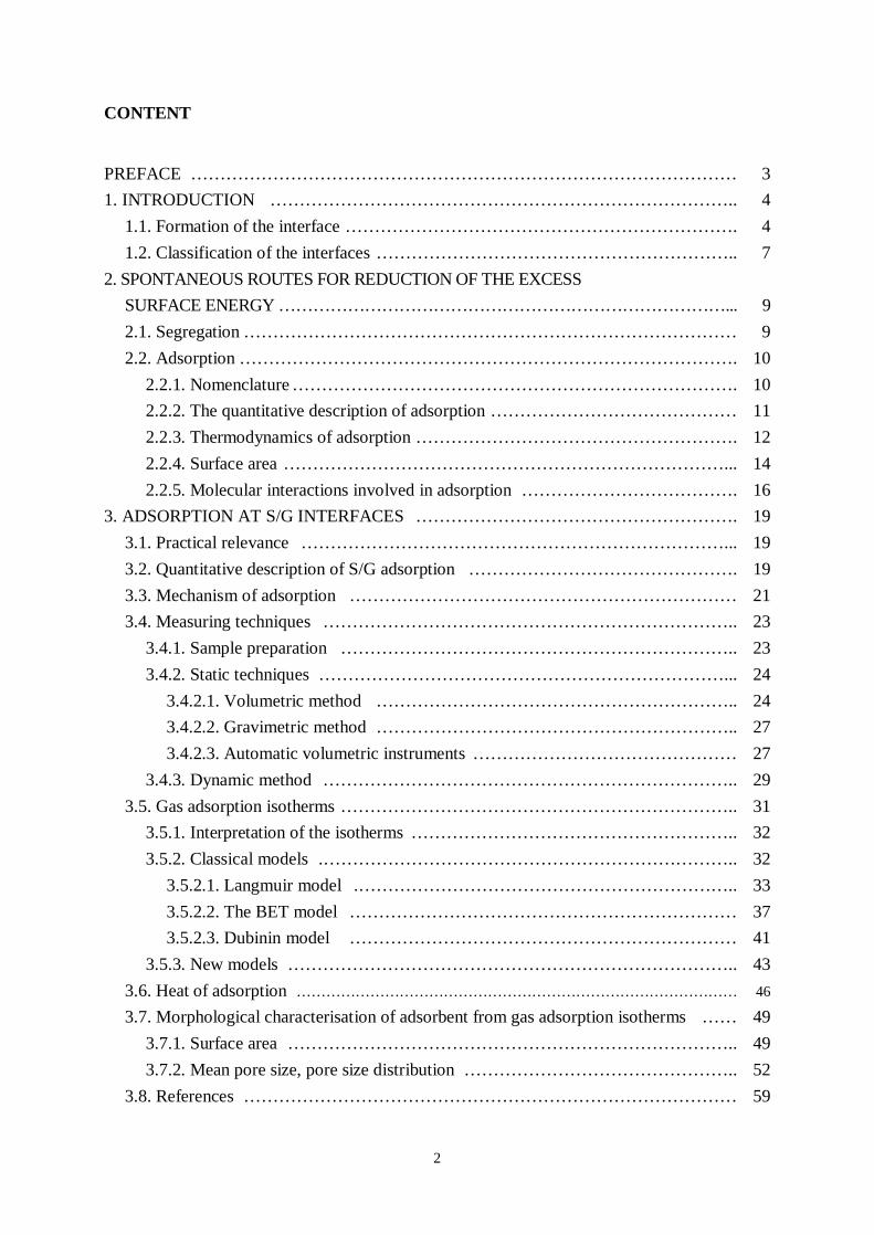
Figure 1.2. In a spontaneous process G is negative. Equilibrium is reached when G = 0.

0G H T S (3)

where H is the change of enthalpy H, S is the change of entropy S and T is the

thermodynamic temperature (in Kelvin). We recall that S is a measure of disorder. When the

more mobile building units (atoms, ions, molecules) of the phase anchor on the surfaces, they

lose part of their freedom, i.e., their entropy decreases, i.e., the TS term in Eq. 3 is negative.

As the process is spontaneous, G is negative. This is possible only if H compensates this

”contradiction”, i.e., it has to be negative. The conclusion is that the adsorption, i.e., the

formation of the interfaces is always an exothermic process. Heat will be generated during

such processes.

The thickness of the layers depends on the physicochemical properties of the adjacent

layers, varying from a few tenths of a nm in the case of a single layer or monolayer (size of a

single atom/ion/molecule) up to 10 - 100 nm. The interface bridges the two adjacent phases: it

separates and simultaneously connects them (Figure 1.3.). The interfacial layer has its own

characteristic physico-chemical data set; however, it is determined by the characteristics of

the parent phases.

7

Figure 1.3. The variation of the physico-chemical properties in the interface.

1.2. Classification of the interfaces

Interfaces may be classified according to

i) the state of the neighbouring phases. From adjoining gas (G), liquid (L) or solid (S)

phases L/G, L/L, S/G, S/l or S/S type interfaces may form. Try to name such interfaces

from your everyday practice.

ii) the geometry of the interface. Flat or curved interfaces may be distinguished. Try to

name such interfaces from your everyday practice.

iii) the energy level(s) of the building units of the interface. Surfaces may be of low or

high energy depending on the energy developed during the formation of the interface

layer. This energy is governed not only by the resultant of the forces acting on the

atoms/ions/molecules in the interface but also by geometric conditions. In particular, in

the case of solid surfaces, surface sites with outstandingly high energy are called active

centres (Figure 1.4.). Very often, this energy is not homogeneous but heterogeneous, i.e.,

it shows a distribution along the surface. The energy and its distribution are one of the

characteristics of the surfaces (Figure 1.5.).

8

a) b) c) d)

Figure 1.4. Geometrically and chemically different active surface sites. a) Geometrically different active sites; b) Sites of identical binding energy (potential) in

atomic resolution. The lines (iso-potential curves) connect sites with identical energy. The distances between the lines represent identical potential differences; c)Chemically different

active sites. The functional groups along the edge of a graphene sheet have a different interaction potential from the carbon atoms in the plane; d) This cartoon by Polányi1

illustrates that the E1 interaction potential of the surface is influenced both by the geometry and the chemical composition of the surface. These potentials level off as we move away from

the surface (X and Y represent different chemical species).

Figure 1.5. Surfaces with various typical energy distributions. kT represents the kinetic energy of an atom/ion/molecule moving freely in the vapour phase at temperature T, k is the Boltzmann constant. The depth of the valleys is proportional to the binding potential of the

surface site. 1 Michael Polanyi, (born as Polányi Mihály in Budapest, 1891 – 1976) was a Hungarian polymath. He made important theoretical contributions to physical chemistry, economics, and philosophy. His wide-ranging research in physical science included chemical kinetics, X-ray diffraction, and adsorption of gases. He pioneered the theory of fiber diffraction analysis in 1921, and the dislocation theory of plastic deformation of ductile metals and other materials in 1934. He emigrated to Germany, in 1926 becoming a chemistry professor at the Kaiser Wilhelm Institute in Berlin, and then in 1933 to England, becoming first a chemistry professor, and then a social sciences professor. (http://en.wikipedia.org/wiki/Michael_Polanyi, 26 January 2014)

9

2. SPONTANEOUS ROUTES FOR REDUCTION OF THE EXCESS SURFACE ENERGY

2.1. Segregation

This process is described in detail in solid state physics. It is of particular significance, e.g., in

polycrystalline materials and alloys. Impurities or additives may congregate in the grain

borders (Figure 2.1.), causing changes in the physico-chemical, mechanical, etc. properties. It

can therefore limit the applicability of alloys as construction materials.

Figure 2.1. At the beginning the impurities/additives are homogeneously distributed in the grain.

For energetic reasons they slowly (solid phase!) congregate on the surface of the grains.

Let us consider the solid alloy of a metal A that contains material B in a low concentration

(additive or impurity). If it is able to form a strong bond on the surface, B will migrate to the

surface. The heats of evaporation, solution and adsorption, respectively, of dopant B are

compared in Figure 2.2. The occurrence of segregation depends on their relative value. In

Figure 2.2 the adsorption heat of B on the surface of metal A exceeds its own heat of

condensation. Therefore, the A-B interactions in the interface are stronger than the B-B

interactions in pure B. This will promote segregation. If the relation of the heats of

condensation and adsorption is reversed, B will migrate (diffuse) away from the grain

boundary. The grain boundary will then be poorer in B than the bulk. It should be kept in

mind that the A-B interaction depends not only of the chemistry of A and B but on the

detailed local morphology/crystallinity conditions as well.

10

Figure 2.2. Comparison of the various heats of phase transition of impurity/dopant B and its heat of interaction with metal A (A-B interactions) [4].

2.2. Adsorption

2.2.1. Nomenclature (Figure 2.3.)

Adsorption is the enrichment of atoms/ions/molecules from a gas, liquid, or dissolved solid to a surface. The process differs from absorption, in which a fluid permeates or is dissolved by a liquid or solid. Adsorption is a surface-based process while absorption involves the whole volume of the material. Desorption is the reverse of adsorption. It is also a surface phenomenon. Adsorption, like evaporation or melting, is an equilibrium process. In equilibrium the amount of adsorbed atoms/ions/molecules is constant. Macroscopically there is no change in the system, but there is a permanent exchange between the adsorbed and free atoms/ions/molecules at a molecular level: adsorption is dynamic. If we consider a solid/gas system, the solid material is called the adsorbent, the gas adsorbed

gas is the adsorbate. The free gas molecules (the potential adsorbates) are called adsorptive.

(Figure 2.3.).

Figure 2.3. Principal terms of adsorption: adsorption, desorption, adsorbent, adsorptive,

adsorbate.

11

2.2.2. The quantitative description of adsorption

For the sake of simplicity let us consider a pure solid – single component gas phase (S/G)

interface at constant temperature. Figure 2.4 shows how the concentration c of the adsorbed

gas changes as we move away from the solid phase. It is assumed that the gas is not absorbed

(!) in the solid phase. Its concentration throughout the solid phase is therefore 0. Quantities

belonging to the surface are distinguished by subscript s.

Figure 2.4. The developing concentration profile of the gas at the S/G interface. t is the

thickness of the adsorbed layer. The area (A+B) is the total amount of the gas in the interface.

The area A is the surface excess amount. Its adsorption is due to the adsorption process,

Area C is the amount of the gas still in the gas phase. cg is the concentration of the free gas.

If we introduce n moles of adsorptive gas over the solid phase, during the adsorption the gas

will be divided between the adsorbed layer of thickness t (ns) and the free gas of volume Vg

(area A+B+C):

sg gn n c V (4)

where cg is the concentration of the non-adsorbed (free) gas in equilibrium (e.g., in mol/l). In

Figure 2.3, the area A shows the real enrichment on the surface, where the area B (the

extension of area C with height cg to beyond t) would exist anyhow. The total amount of the

gas in the interface layer ns can also be expressed with the volume Vs of the layer:

ss

gn c V n (5)

12

Therefore, n corresponds to area A (the superscript will be used to distinguish quantities

corresponding to the surface excess). The surface excess amount building up during the

adsorption can be given as

0

( )SV

s sg gn n c V c c dV (6)

where c is the concentration of the gas at any point in the adsorbed layer. Note that if the

value of cg is sufficiently small

sn n . (7)

2.2.3. Thermodynamics of adsorption

The thermodynamic potential functions internal energy U, enthalpy H, entropy S, the

Helmholtz free energy A and the Gibbs free energy G belonging to the adsorption process can

be given as

gas solidU U U U (8)

gas solidH H H H (9)

gas solidS S S S (10)

gas solidA A A A (11)

gas solidG G G G (12)

For the sake of clarity, we use the full name of the solid and gas phases in the indices. As an

example, Ugas and Usolid are the internal energies of the gas and solid phases, respectively,

before the adsorption. U is the internal energy of the total system after the adsorption. Their

difference defines the change in internal energy due to the adsorption (excess internal energy

of the adsorption U).

The thermodynamic condition of the adsorption equilibrium

Due to the adsorption process

0dn > (13)

and

gassn n n n .

(14)

13

As gas adsorption measurements are most often performed at constant volume, the Helmholtz

free energy functions will be used for the description. Similarly to Figure 2, in equilibrium

, , ,

0 sT V A n

An (15)

where T, V and As are the temperature, the volume of the system, and the surface area of the

solid material exposed to the gas (s is subscript!).

Using Eq. 11 the Helmholtz free energy of the system after the adsorption is

, , , , ,,

0sgas olid

ss sT V A n T T V TA A

AA An n

Ann

(16)

If no change occurs in the solid phase during the adsorption (no absorption) the ,

solid

sT A

An

term of Eq. 16 is 0, i.e., the adsorption does not modify the free energy of the solid phase.

In a closed system

0gasdn dn dn . (17)

Thus

,, ,

gas

s

gas

gas T VT A T V

A AAn nn

. (18)

Or with the usual symbol of the chemical potential

gas . (19)

That is, the equilibrium is established, when the free energy (chemical potential) of the gas in

the free gas phase and in the adsorbed layer becomes equal.

14

2.2.4. Surface area

Taking advantage of the adsorption (surface enrichment) phenomenon requires a large

number of molecules in the outermost layer of the solid material, i.e., a large contact area

between the adjacent phases. (It also means that high surface area materials are more sensitive

to their environment.) The contact area can be increased, e.g., by milling the solid or using it

in a porous form.

In the case of solids the measure of the contact area is the specific surface area, i.e.,

the surface area generally of 1 g solid:

surface areamass of the solidsA (20)

most often given in m2/g units. Unless otherwise stated the term surface area means specific surface area, as it is the generally used term for it in the scientific communications. If high surface area is reached by milling the solid into particles in the nanometer range (1 nm=10-9 m), this leads to the appearance of specific features not experienced with bulk materials. Making use of such extreme features is the objective of nanotechnologies. For tiny spherical particles of diameter d the relationship between the surface area and the particle size can be given as

6s

abszolút

Ad

, (21)

where abs is the real density of the solid matrix (density of the skeleton of the solid material). Figure 2.5 illustrates the dramatic increase of the molecules in surface position as the particle size decreases towards the nanosize range (note the logarithmic horizontal scale).

Figure 2.5. The ratio of the atoms/ions/molecules in surface position depends on the particle

diameter d (in case of a silica, SiO2, where the molar volume is Vm 30 cm3/mol).

15

The form of high surface area porous materials can be very diverse. Bricks, toilet-sponges and

soil, e.g., belong to this group of materials. In most cases their external surface area is not

particularly high (Figure 2.6.), but the pores allow access to the internal surfaces.

Figure 2.6. Distinction between external and internal surface areas.

In addition to their high surface area, they also can be characterized by their porosity ,

defined as

pore abs apparent

pore solid abs

VV V

(22)

where Vpore and Vsolid are the volumes of the accessible pores and of the solid matrix,

respectively. abs was defined earlier, apparent is the apparent or bulk density of the solid

material (the mass of a given volume of the solid). The absolute density is generally measured

by gas (preferably helium) pycnometry.

In their appearance pores may be very different: open, dead-end, closed, independent,

networking, etc. Figure 2.7 illustrates such possibilities. It also shows that pores may also be

formed as interparticle space through aggregation of nonporous particles.

Figure 2.7. Pores of various shapes and connectivity.

16

Besides their shape and accessibility pores are classified by their size. The pore

categories established by International Union of Pure and Applied Chemistry (IUPAC) are the

following:

macropores: width exceeding 50 nm,

mesopores: width in the range 2–50 nm,

micropores: width narrower than 2 nm.

Later we will realise that these seemingly arbitrary sizes are strongly related to the

adsorption mechanism of gas molecules.

Outstandingly high surface area materials are porous and their typical pore size lies in

the micropore range.

2.2.5. Molecular interactions involved in adsorption

On the molecular level adsorption interactions can be described as the total of dispersion

attraction and short range repulsion potentials of the electron clouds of the approaching

particles. The attractive London dispersion potential EA between two particles separated by a

distance r can be expressed as

6ACE ( r )r

, (23)

where C is a parameter defined by the polarizability of the two approaching atoms. The

repulsion term ER is

( )R m

BE rr

(24)

B and m are empirical parameters. m is very often taken to be 12. The total potential,

6 12

C BE( r )r r

(25)

is the so called 12-6 Lennard-Jones potential. This function is the one most frequently used

for theoretical calculations and simulation of adsorption processes.

17

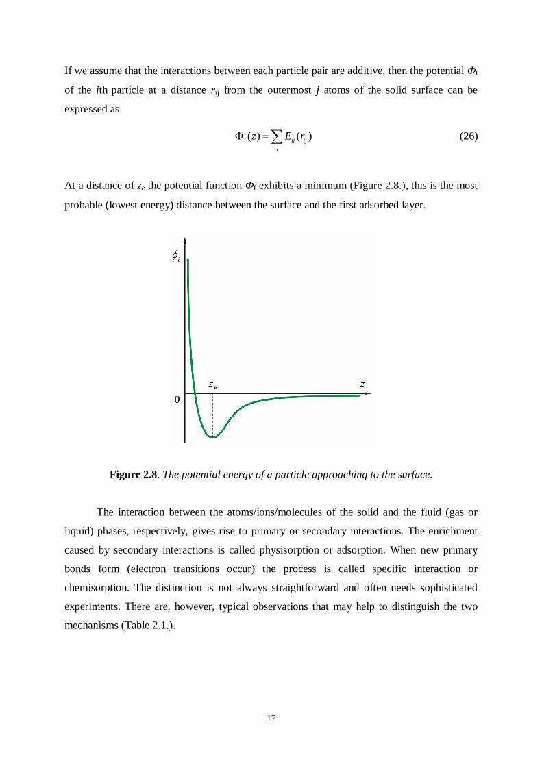
If we assume that the interactions between each particle pair are additive, then the potential I

of the ith particle at a distance rij from the outermost j atoms of the solid surface can be

expressed as

( ) ( )i ij ijj

z E r (26)

At a distance of ze the potential function I exhibits a minimum (Figure 2.8.), this is the most

probable (lowest energy) distance between the surface and the first adsorbed layer.

Figure 2.8. The potential energy of a particle approaching to the surface.

The interaction between the atoms/ions/molecules of the solid and the fluid (gas or

liquid) phases, respectively, gives rise to primary or secondary interactions. The enrichment

caused by secondary interactions is called physisorption or adsorption. When new primary

bonds form (electron transitions occur) the process is called specific interaction or

chemisorption. The distinction is not always straightforward and often needs sophisticated

experiments. There are, however, typical observations that may help to distinguish the two

mechanisms (Table 2.1.).

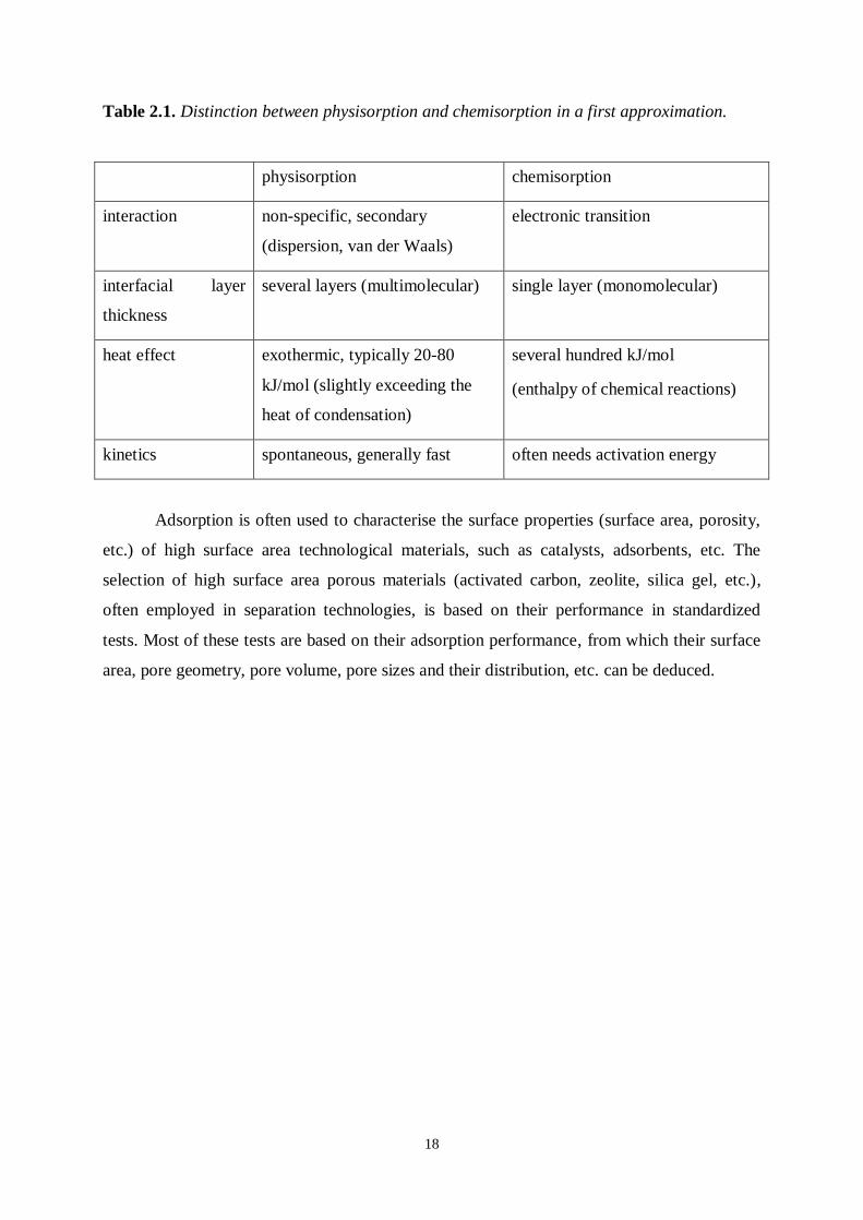
18

Table 2.1. Distinction between physisorption and chemisorption in a first approximation.

physisorption chemisorption

interaction non-specific, secondary

(dispersion, van der Waals)

electronic transition

interfacial layer

thickness

several layers (multimolecular) single layer (monomolecular)

heat effect exothermic, typically 20-80

kJ/mol (slightly exceeding the

heat of condensation)

several hundred kJ/mol

(enthalpy of chemical reactions)

kinetics spontaneous, generally fast often needs activation energy

Adsorption is often used to characterise the surface properties (surface area, porosity,

etc.) of high surface area technological materials, such as catalysts, adsorbents, etc. The

selection of high surface area porous materials (activated carbon, zeolite, silica gel, etc.),

often employed in separation technologies, is based on their performance in standardized

tests. Most of these tests are based on their adsorption performance, from which their surface

area, pore geometry, pore volume, pore sizes and their distribution, etc. can be deduced.

19

3. ADSORPTION AT S/G INTERFACES

3.1. Practical relevance

Physico-chemical interactions at S/G interfaces are of great practical importance. Such

processes take place spontaneously and continuously, e.g., in nature and in the environment.

The interaction of building materials with corrosive pollutants weakens their mechanical

properties, or results in changes in surface properties (e.g., ageing of metal surfaces, corrosion

of marble statues, etc.) that can be either desired or undesired. In air, the interaction between

fine solid particles (e.g., dust, soot) and pollutants (e.g., NOx, CO, SOx, flue gas, water and

organic vapour) may influence the mobility of airborne particles by changing their surface

properties. On the other hand, these interactions could be utilized in smaller or larger scale

technologies for removing volatile pollutants or separating the various components of a mixed

gas phase. S/G adsorption plays a fundamental role in separation technologies, analytical

methods, characterization of solid materials and in materials science. Only a few examples are

given here. Gas purification technologies, such as the separation of various gas mixtures (air,

flue gas) are based on the selective adsorption of their components. The sorption capacity of

the filled column, or the heat evolved during adsorption cycles are important parameters in the

design of gas separation/purification columns. The widely known analytical method of gas

chromatography is also based on this phenomenon. In efficient gas storage (e.g., hydrogen,

methane, CO2, etc.) technologies, which are attracting increasing attention, the pore volume of

the adsorbent and the geometry of the pores are crucial parameters. The selectivity and the

strength of the adsorption at S/G interfaces are essential in the development of good

heterogeneous catalysts.

Several parameters widely used for characterising high surface area materials, either

porous or non-porous, such as surface area, pore volume, pore size and shape, pore

accessibility, energy (and energy distribution) of the surface sites, mechanism and kinetics of

the interactions, etc., are derived by measuring the S/G interactions under controlled

conditions.

3.2. Quantitative description of S/G adsorption

The measure of adsorption can be either the total or the excess amount of the gas (this

distinction was made in the previous chapter) attracted by a unit mass m of the solid. The

amount of the gas can be expressed in several ways. In chemistry we prefer to express these

amounts in moles, Ns and N, respectively.

20

or s

s N Nn nm m

(27)

Instead of the number of moles we could equally well use the mass of the adsorbed gas, the

volume of the gas (this requires the temperature and pressure of the gas to be specified), or the

volume of the liquefied gas. In what follows, however, unless otherwise stated, we use molar

quantities.

We recall that according to the kinetic theory of gases, the velocity v of the gas

atoms/molecules depends on the temperature T:

3 kTvm

(28)

k is again the Boltzmann constant and m is the mass of the gas particle. Therefore, the lower

the temperature the higher is the probability of adsorption, i.e., the probability that when the

gas particles strike the surface, they remain adsorbed. The fate of a bombarding gas

atom/molecule in the collision is determined principally by the relation between its kinetic

energy (see Eq. 28) and the energy released by its adsorption. Systematic measurements to

determine the adsorbed amount are most often performed at constant temperature (Figure

3.1). (As adsorption is an exothermic process the system should be thermostated.) The amount

of gas adsorbed is measured as a function of the concentration c (i.e., equilibrium pressure p)

of the free (non-adsorbed) gas:

( )sTn f c or ( )s

Tn f p , (29)

This function is called the adsorption isotherm. Very often, as in Eq. 29, the adsorbed

amount is referred to the mass of the solid material. The limit of p is the saturation pressure p0

of the gas at temperature T. A relative pressure can be defined as p/p0. Isotherms are often

represented as 0( )sTn f p/p . A complete adsorption isotherm can be obtained when p/p0 is

systematically increased from 0 up to 1. (When p/p0=1 is reached condensation occurs even

on a planar surface!) If we “turn back” after reaching the end of the adsorption isotherm and

systematically reduce the equilibrium p/p0, we obtain the desorption isotherm. When the

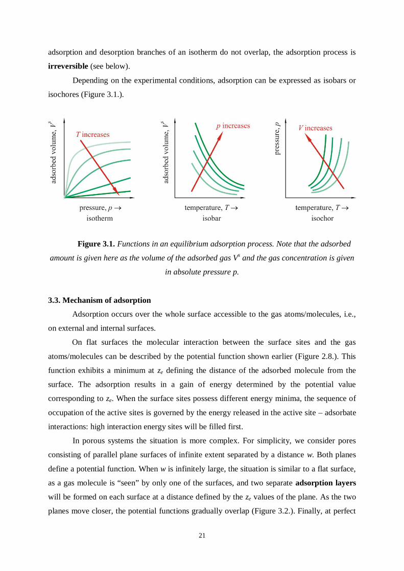
21

adsorption and desorption branches of an isotherm do not overlap, the adsorption process is

irreversible (see below).

Depending on the experimental conditions, adsorption can be expressed as isobars or

isochores (Figure 3.1.).

Figure 3.1. Functions in an equilibrium adsorption process. Note that the adsorbed

amount is given here as the volume of the adsorbed gas Vs and the gas concentration is given

in absolute pressure p.

3.3. Mechanism of adsorption

Adsorption occurs over the whole surface accessible to the gas atoms/molecules, i.e.,

on external and internal surfaces.

On flat surfaces the molecular interaction between the surface sites and the gas

atoms/molecules can be described by the potential function shown earlier (Figure 2.8.). This

function exhibits a minimum at ze defining the distance of the adsorbed molecule from the

surface. The adsorption results in a gain of energy determined by the potential value

corresponding to ze. When the surface sites possess different energy minima, the sequence of

occupation of the active sites is governed by the energy released in the active site – adsorbate

interactions: high interaction energy sites will be filled first.

In porous systems the situation is more complex. For simplicity, we consider pores

consisting of parallel plane surfaces of infinite extent separated by a distance w. Both planes

define a potential function. When w is infinitely large, the situation is similar to a flat surface,

as a gas molecule is “seen” by only one of the surfaces, and two separate adsorption layers

will be formed on each surface at a distance defined by the ze values of the plane. As the two

planes move closer, the potential functions gradually overlap (Figure 3.2.). Finally, at perfect

22

overlap a single minimum is reached. This situation is strongly influenced by the size of the

probe molecules approaching the surface, as illustrated in Figure 3.2.

Figure 3.2. Variation of the overlap of the adsorption potentials in slit shaped pores

consisting of identical parallel walls. and * are the adsorption potentials in the pore and

over a free flat surface, respectively. w is the width of the pore and d is the diameter of a

spherical probe atom/molecule (after [2]).

It can be concluded that over flat surfaces or in pores that are significantly wider than

the size of the probe molecule, adsorption occurs in well-defined layers. In the case of gases

this happens typically in mesopores and macropores. When the pore size w does not exceed

2d (for gases in micropores), volume filling or pore filling is the typical adsorption

mechanism. The narrower the pore, the deeper is the potential well. Figure 3.3 demonstrates

the adsorption mechanism of nitrogen molecules ( 0.35 nmd ) at 77 K (the boiling point of

liquid nitrogen).

23

Figure 3.3. Adsorption mechanism of N2 molecules at 77 K in pores of different widths

(represented by the V shape of the pores) and the development of pore filling as the

adsorption progresses (the equilibrium p/p0 increases) (After [3]).

3.4. Measuring techniques

Gas adsorption isotherms can be obtained by static or dynamic (flow) techniques. The

static method can be either volumetric (the volume of the adsorbed gas is deduced by

measuring the pressure drop in a constant volume space) or gravimetric (the adsorbed gas

increases the mass of the sample, which is measured with a very sensitive balance). Collecting

the data points of an equilibrium adsorption isotherm needs carefully controlled experimental

conditions and measurements). Sample preparation (desorbing all surface contamination) and

the establishment of the consecutive equilibrium states throughout the adsorption and

desorption branches of the isotherm can last several days.

3.4.1. Sample preparation

When a solid surface is exposed to a gas at pressure p and temperature T, the number

of the collisions with the surface can be calculated from the kinetic theory of gases. It is

2pNmkT

. (30)

where m is the mass of the gas atom/molecule. According to this expression at ambient

pressure each cm2 of a surface is exposed to 3·1023 collisions. If we assume 1015 atoms on a

24

surface of 1 cm2, the frequency of the collisions is about 108/s. Generally, at ambient

conditions and atmospheric pressure, all surfaces are covered by physisorbed or even

chemisorbed (e.g. water!) impurities. Reducing the pressure and/or increasing the temperature

fosters the removal of these contaminants (Figure 3.4.). The temperature, however, is limited

by the thermal sensitivity of the solid matrix or the functional groups that decorate its surface.

Figure 3.4. Contamination can be effectively removed by combined thermal and vacuum

treatment of the adsorbent.

The quality of the vacuum applied during the sample preparation not only influences

the purity of the surface after the treatment but also limits the first (lowest pressure) point

obtained in the subsequent measurement.

3.4.2. Static techniques

3.4.2.1. Volumetric method

For a given adsorbent – adsorptive system the amount of adsorbed gas (the amount of the

adsorbate) depends on the pressure and the temperature. After careful sample preparation the

adsorbent is transferred into a space of volume V and thermostated to temperature T. The

construction of a classical instrument made of glass is shown in Figure 3.5. (The name

“volumetric” comes from the experimental practice, as the amount of the adsorbed gas was

read as volume from the gas burette.) For the first point the system is evacuated. Introducing a

given amount of gas into this otherwise sealed space, the pressure of the gas will gradually

decrease due to its enrichment at the surface (the amount of the free gas decreases) until the

equilibrium state is established. Then a new pulse of gas is introduced and the equilibration

starts again.

25

Figure 3.5. Principle of the volumetric method. The amount of adsorbed gas is determined

from the position of the mercury level in the gas burette. When the equilibrium state is

reached the corresponding pressure is read from the position of the mercury manometer

(after [3]).

Such home-made manual experimental setups have been gradually replaced by commercially

available automatic instruments. The quality of the experimental data depends on the stability

of the temperature, the establishment of the state of equilibrium (often time consuming), the

determination of the volume V of the space where the adsorption takes place and the accuracy

of the pressure reading. (The latter depends strongly on V as the pressure change is more

pronounced if the same amount of gas is “removed” by adsorption from a smaller space.)

The sample holder is thermostated at temperature T. When N moles of gas are

introduced into the adsorption chamber of volume V the expected pressure pexpected can be

calculated from the appropriate gas law. Since part of the gas adsorbs on the surface, the

amount 'N N of gas still filling freely the space can be deduced from the measured

equilibrium pressure e expectedp p .

The difference ( ')N N defines the amount of gas “removed” by the adsorption:

( ')sN N N (32)

26

By repeating these steps the complete function Ns = f(pe) can be determined (in both

directions). If the mass m of the adsorbent (after outgassing prior to the adsorption

measurement) is known, the specific adsorption can be calculated (Eq. 27). Generally, data

are displayed in the form ns = f(p/p0) (e.g., in mol/g), where p/p0 here is the relative

equilibrium pressure.

For the sake of simplicity, and to illustrate the significance of the volume throughout

the series of equilibrium measurements, here we use the ideal gas law

' ep VNRT

(33)

As V is used in each step of the calculation of the current value of N’, it can be a source of

systematic error. In other words, we must know exactly the volume of the constant space in

which the adsorption occurs. Commercial instruments employ two approaches. A sample

holder of calibrated volume is used. However, the sample itself occupies part of this space.

This problem is overcome easily if the true density of the solid sample is determined in an

independent experiment, or is known from the literature. Another option is to determine V at

the start of the experiment by introducing helium into the cell that also contains the outgassed

sample. As helium starts to physisorb only close to its extremely low boiling point, only space

filling occurs and V can be derived directly from the measured pressure.

The volumetric method is usually employed in low temperature measurements (the

boiling point of the liquefied gas is below ambient temperature). The stability of T is ensured

by using the phase transition of a carefully selected liquid, preferably the liquid form of the

adsorptive itself. The most frequently employed cooling media are nitrogen (boiling point 77

K), argon (boiling point 87 K), ice/water (melting point 273 K).

27

3.4.2.2. Gravimetric method

Figure 3.6. Principle of the gravimetric method. The amount of adsorbed gas is determined

from the elongation of a sensitive spring. Its response to load is calibrated in independent

measurements (after [3]).

The scheme of the classical McBain balance is shown in Figure 3.6. The adsorption process is

recorded by measuring the mass of the sample after evacuation of the system. If corrections

for buoyancy as a source of systematic error are taken into account the sensitivity can be as

high as 0.1 µg. Nowadays the spring is replaced by a single crystal balance. The gravimetric

technique is preferred for ambient temperature measurements (e.g., uptake of organic vapours

around room temperature).

3.4.2.3. Automatic volumetric instruments

Computer controlled automatic instruments that are now commercially available

employ one of the operational principles described above. Data collection is automatic. The

scheme of one such instrument is shown in Figure 3.7. Values of the desired equilibrium

pressure at almost ambient density, as well as the equilibrium criteria, can be pre-set by the

software provided. The equilibrium pressure is selected by the pressure profile, which is

closely tracked. A typical set of pressure profiles is shown in Figure 3.8. The time delay

28

between successive pressure measurements after each gas injection can be adjusted. The

equilibrium pressure is established when the pressure difference of two subsequent electronic

readings for a pre-set time does not exceed a pre-set difference. Longer pre-set times and

smaller pre-set differences mean more accurate but longer measurements. These values can be

optimized by the user.

In addition to automatic data collection, commercial instruments provide permanently

updated series of data evaluation software(s). The role of the user is to select the best or

optimized model for the materials investigated from among the programs available.

Figure 3.7. Flow diagram of an automatic static volumetric gas adsorption instrument. Legend: lights

numbered from 1-11 show the position of the valves separating various units of the instrument (green:

valve open, red: valve closed); ADS – adsorptive inlet (nitrogen); VAC – vacuum pump with coarse

(3) and fine (4) options; He – auxiliary helium gas inlet; DEGASSER 1 and 2 –simultaneous

preparation of two samples, combined with heaters (max. 300 °C); COOLANT – shows that the

sample is immersed in liq. nitrogen; ANALYSIS – samples A and B can be measured simultaneously;

VENT – rinsing gas outlet.

29

Figure 3.8. Variation of the pressure profile during the adsorption and desorption

steps.

3.4.3. Dynamic method

The dynamic method is a relatively fast technique. It is preferred to prompt estimation

of the surface area from a single point measurement. A further advantage is that it does not

require a vacuum system. The sample may be pre-treated in an inert gas flow at ambient or

elevated temperature. During the measurement a two-component gas mixture flows through

the sample at two different temperatures. One of the components is the carrier gas (generally

He or H2), which is not adsorbed at either of the temperatures applied. The adsorption of the

other component (probe gas, most often N2) is reversible and depends strongly on the

temperature (Figure 3.8.). Typically, the gas mixture contains 30 % (v/v) nitrogen and 70 %

(v/v) carrier gas.

The signal is generated by the composition difference of the gas flowing in the two

branches. An advantage of these mixtures is that they can easily be monitored by thermal

conductivity detectors. The adsorbed amount is proportional with the integral of the signal.

At the beginning of the experiment the sample holder containing the pretreated solid is

immersed in water at ambient temperature. Neither of the components of the binary gas

mixture adsorbs at this temperature. The composition of the gas mixture in the two branches

is identical. In order to calibrate the system we inject a known amount of nitrogen into the

sample branch. It passes through without adsorption, but increases the concentration

temporarily (peak 1 in Figure 3.9.). Then the water bath is substituted by liquid nitrogen. At

this temperature the nitrogen component adsorbs, generating a negative deviation in the signal

30

(peak 3). After the adsorption is complete the sample is returned to the water bath (region 4).

Then reversible desorption of the nitrogen gas takes place, which gives rise to an increase of

nitrogen concentration in the mixture (peak 5). For metrological and kinetic reasons this peak

is used for the evaluation of the adsorption performance of the sample.

Figure 3.8. Instrument for dynamic adsorption measurement (after [3])

Figure 3.9. Concentration response during a dynamic adsorption measurement. 1:

calibration peak, 2 contraction (due to transfer into the liquid nitrogen bath), 3) adsorption

peak, 4 transfer into water bath, 5 desorption peak.

31

3.5. Gas adsorption isotherms

The shape of the 0( / )sTn f p p functions and the numerical values obtained with a

system are defined by the physico-chemical behaviour of the components and the interaction

between the adsorbent and the adsorbate. (From this point on we omit the subscript e

previously used to distinguish the equilibrium conditions.) Several different systems exist for

classifying gas adsorption isotherms, based on a large number of experimental observations.

Here we discuss the classification established by International Union of Pure and Applied

Chemistry (IUPAC) 2.

According to the shape of the isotherm (initial slope of the curves, the overlapping of the

adsorption/desorption branches, etc.), six types are distinguished (Figure 3.10). Each

shape/type represents a set of characteristics that typify both the solid and the gas phases and

their interaction.

Figure 3.10. IUPAC classification of gas adsorption isotherms. As noted in the text, the adsorbed amount can be expressed in molar or mass bases, or as the volume of the adsorbed

gas or its liquid equivalent. When adsorbed gas volume is used, the corresponding temperature and pressure must be specified.

Type I: This is typical when physisorption takes place on microporous materials with low

external surface area (e.g., activated carbons, zeolites, molecular sieves, certain porous metal

oxides). The narrow micropores become saturated already at low relative pressure. This shape

is typical in chemisorption. 2 IUPAC is an international federation of chemists. IUPAC is best known for its work in standardizing nomenclature in chemistry and other fields of science. It releases publications in many fields including chemistry, biology and physics. IUPAC is also known for standardizing the atomic weights of the elements [http://en.wikipedia.org/wiki/International_Union_of_Pure_and_Applied_Chemistry. 27 January, 2014].

32

Type II: Represents reversible adsorption, typically on the surface of nonporous or

macroporous materials. The adsorption occurs through layer formation. The point B is the

inflection point of the knee, which corresponds to completion of the monolayer (see below).

Type III: The adsorption is reversible, but the isotherm is convex throughout the whole p/p0

range. This indicates a weak interaction between the adsorbent and the adsorbate (a typical

example is the adsorption of polar water on the surface of pure graphite). Therefore, the

adsorptive – adsorptive as well the adsorbate – adsorbate interactions govern the adsorption

mechanism.

Type IV: The adsorption process is irreversible, since the adsorption and desorption branches

do not overlap. Its special feature is the hysteresis loop. Typical in case of mesoporous

adsorbents.

Type V: The sorption is irreversible, but the adsorbent – adsorbate interaction is weak as in

the case of Type III. It is typical when water is adsorbed by a porous nonpolar material.

Type VI: Stepwise isotherm. It occurs, e.g., when multilayer adsorption of spherical

atoms/molecules take place on a well ordered surface. Example: adsorption of krypton or

argon (nonpolar atoms) on the surface of graphitic carbon at 77 K.

3.5.1. Interpretation of the isotherms

Adsorption measurements are mostly performed to investigate the surface properties

of the adsorbent. Based on the long term experience quintessential to the classification,

general information can be deduced from the shape of the isotherm itself: the type of the

isotherm, the reversible/irreversible character of the adsorption, the slope of the initial section.

The total pore volume can be deduced from the endpoint of the isotherm at 0/ 1p p .

With the help of adsorption models more information can be extracted about the

surface area, the heat of adsorption, the shape, the average size and the size distribution of the

pores, etc.

3.5.2. Classical models

The large number of widely used models available for interpreting adsorption data

implies that there is as yet no model that fits all systems, or that interprets the isotherm over

the whole relative pressure range 0 – 1. Applicability of the models is often limited to

particular systems, or is valid only in a certain p/p0 range. The most widely used models will

be discussed in the following sections.

33

3.5.2.1. Langmuir model

This model was developed by Irving Langmuir3 in 1916.

The two hypotheses of this simple model (Figure 3.11.) are

i) the surface is energetically homogeneous (all the surface site – probe molecule

interactions yield the same adsorption energy);

ii) adsorption is limited to a single layer (monolayer)

Figure 3.11. The Langmuir model. Nm is the total number of sites, Ns the number of the

occupied sites. The coverage is limited to a closely packed single layer.

One of the consequences of these conditions is that the lateral interaction between the adsorbates is neglected, i.e., the adsorptive atoms/molecules may land randomly on the free sites of the surface until a closely packed monolayer is complete. Owing to its incompressibility, this monolayer can be considered as a liquid film with a thickness of a single molecule. As it was also assumed that adsorption occurs only on well-defined sites of the sample surface

(one per molecule, Figure 24) the process can be described by the following simple chemical

equation:

A(gas) S AS

where A(gas) is the free adsorptive in the gas phase, S is an active site of the surface and AS is

the adsorbate already anchored to the surface site. The double arrow indicates that adsorption

is an equilibrium process. If Ns surface sites are already occupied out of the total number Nm,

then the surface coverage can be given as 3 Irving Langmuir (1881 –1957) was an American chemist and physicist. He advanced several basic fields of physics and chemistry, and was awarded the 1932 Nobel Prize in Chemistry for his work on surface chemistry. Langmuir, the journal of the American Chemical Society for Surface Science, was named in his honour [http://en.wikipedia.org/wiki/Irving_Langmuir. 28 January 2014].

34

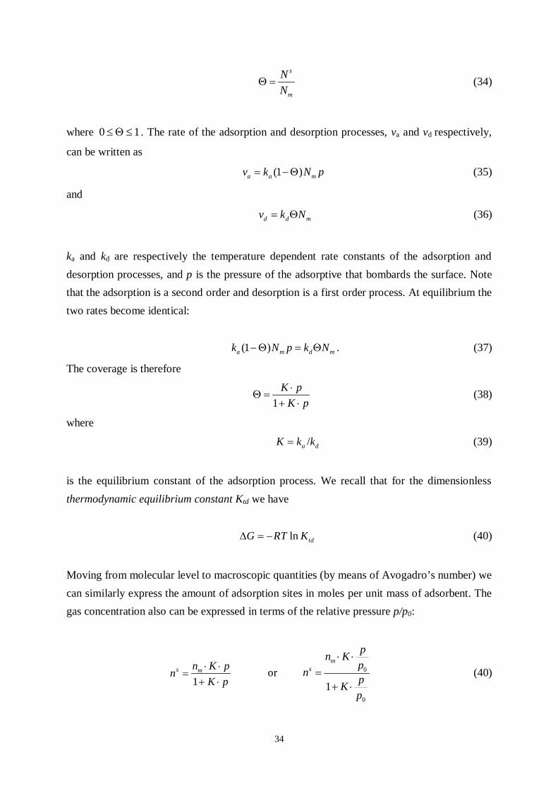
s

m

NN

(34)

where 0 1 . The rate of the adsorption and desorption processes, va and vd respectively,

can be written as

(1 ) a a mv k N p (35)

and

d d mv k N (36)

ka and kd are respectively the temperature dependent rate constants of the adsorption and desorption processes, and p is the pressure of the adsorptive that bombards the surface. Note that the adsorption is a second order and desorption is a first order process. At equilibrium the two rates become identical:

(1 )a m d mk N p k N . (37)

The coverage is therefore

1K p

K p

(38)

where

/a dK k k (39)

is the equilibrium constant of the adsorption process. We recall that for the dimensionless thermodynamic equilibrium constant Ktd we have

ln tdG RT K (40)

Moving from molecular level to macroscopic quantities (by means of Avogadro’s number) we can similarly express the amount of adsorption sites in moles per unit mass of adsorbent. The gas concentration also can be expressed in terms of the relative pressure p/p0:

1s mn K pn

K p

or 0

0

1

ms

pn Kpn pKp

(40)

35

ns is the specific adsorbed amount (e.g., in mol/g) and nm is the amount needed to complete

the closely packed monolayer on the surface (e.g., in mol). The shape of Eq. (40) is shown in

Figure 3.12.

Figure 3.12. Shape of a typical Langmuir isotherm.

1

s

m

n K pn K p

or 0

0

1

s

m

pKpn

pn Kp

(41)

is plotted in Figure 3.13. The greater the value of K (the larger the gain of G) the steeper is

the initial section of the isotherm.

Figure 3.14. The influence of the K parameter on the shape of the Langmuir isotherm.

At low pressure ( 0p ) Eq. 40 simplifies to the linear form

36

sm Hn n K p K p or

0 0

sm H

p pn n K Kp p

(42)

i.e., to the Henry4 isotherm. The adsorption is directly proportional to the gas concentration

and the proportionality factor is the Henry adsorption constant KH. This implies that that K

and nm cannot be defined separately.

In Eq. 40 the equilibrium pressure p (or p/p0) and ns are obtained from adsorption

measurements, and K and nm are the fitting parameters of the Langmuir model. The two latter

are generally deduced from the so-called linear Langmuir plot. Eq. 40 can be rearranged to

give

1s

m m

p pn Kn n

(43)

Instead of plotting ns against p/p0 (Figure 3.13), / sp n is plotted on the ordinate (vertical) axis.

Linearity of the plot can mean that the model is applicable to the system studied. The

Langmuir parameters can be obtained from the slope and the intercept of the fitted straight

line, as shown in Figure 3.15.

Figure 3.15. Derivation of the Langmuir parameters from linear Langmuir plot.

A great advantage of the Langmuir model is that it is based on a clear and simple

physical model and its parameters can therefore be related directly to this physical picture. On

4 William Henry (1774 –1836) was an English chemist.

37

the other hand its applicability is in practice quite limited for gas adsorption. Its most serious

weaknesses are

i) identical adsorption energy of the active sites,

ii) neglect of lateral interactions between the adsorbates, and

iii) limitation of the thickness of the adsorption to a single layer. In most cases (except

in chemisorption) multilayers develop when 0/ 0.05p p . The best fit is achieved when the

adsorption data provide a shape of Type I (the process is chemisorption or the adsorbent

contains exclusively micropores).

3.5.2.2. The BET model

Probably the most widely known and applied model for the evaluation of gas

adsorption data. The Brunauer–Emmett–Teller (BET) theory serves as the basis of an

important analysis technique for measuring the specific surface area of a material. It was

published first in 1938 by Stephen Brunauer, Paul Hugh Emmett, and Edward Teller5. Their

concept extended the Langmuir model to multilayer adsorption using the following

assumptions:

(i) gas molecules physically adsorb on the solid surface in an infinite number of

layers;

(ii) there is no interaction between the adsorbed layers; and

(iii) the Langmuir theory can be applied to each layer.

The multilayer gas molecule adsorption considered in this model does not require a layer to be

complete before an upper layer formation starts (Figure 3.16.a).

Further assumptions involved in their model:

i. An already adsorbed molecule (adsorbate) can act as a single adsorption site for a

molecule in the upper layer.

ii. The uppermost adsorbed layer is in equilibrium with the free gas phase, i.e., the rates of

adsorption and desorption are identical.

iii. Desorption is a kinetically controlled process, i.e., energy has to be provided:

- the energy is identical for each molecule of the same layer

- for the first layer it is the same as (-1) the heat of adsorption at the solid surface

5 S. Brunauer, P. H. Emmett and E. Teller, J. Am. Chem. Soc., 1938, 60, 309. Stephen Brunauer (Hungarian: Brunauer István, 1903 – 1986) was a Hungarian born American physico-chemist. Paul Hugh Emmett (1900 – 1985) was an American chemical engineer. Edward Teller (Hungarian: Teller Ede; 1908 – 2003) was a Hungarian-born American theoretical physicist.

38

- all the other layers are similar and can be represented as the liquid state (the

adsorbing molecule transfers from the gas phase to the adsorbed layer, which can

be considered as being incompressible, i.e., liquid). Thus, the energy required is

the heat of evaporation, EL, independently of how far the layer is from the solid

surface.

iv. When the saturation pressure is reached, the number of adsorbed layers tends to

infinity (i.e. it is assumed that the sample is surrounded by a liquid phase).

a b

Figure 3.16. Multilayer adsorption (a) and its physical model (b) according to the

hypothesis of Brunauer, Emmett and Teller. N0, N1, N2, etc. … are the number of molecules in

the corresponding layers.

The chemical formalism of such adsorption can be given as

A(gas) S AS

A(gas) AS A2S

A(gas) A2S A3Setc.

For the first equation describing the adsorption on the clean solid surface the rate of

adsorption is

0a av k N p (44)

and that of desorption 1d dv k N (45)

39

N0 and N1 are the number of active sites on the surface and in the first adsorbed layer,

respectively. ka is the adsorption and kd the desorption rate constant, p is the equilibrium

pressure of the free gas.

From the equilibrium criteria

0 1a dk N p k N (46)

For the second layer

' '1 2a dk N p k N (47)

Generally ' '

1 a i d ik N p k N (48)

where i= 2, 3, etc., Ni is the number of molecules in the i-th layer and the values of 'ak and '

dk

are respectively assumed to be similar for the adsorption and desorption processes in all the other layers. Their temperature dependence can be given by the Arrhenius law:

exp aa

EkRT A and ' exp L

aEkRT (49)

where Ea is the heat of adsorption of the first layer and EL is the heat of condensation of the gas. The derivation of the model equation is more complex than for the Langmuir model. Further details are given, e.g., in [3]. The resulting BET equation is

0

00

1 ( 1)1

sm

ppCn n pp C

pp

, (50)

Like Langmuir’s model, it has two parameters, the monolayer capacity nm and an energy term

/netQ RTC e characterizing the overall interaction between the gas and the solid. Qnet is the net

heat of adsorption net a LQ E E . In Figure 3.17 isotherms of different C values are

compared. We recall that the steeper the initial section of the isotherm the stronger is the adsorption interaction, i.e., a high C value. This requires a large Qnet, i.e., a substantial

difference between aE and LE .

40

Figure 3.17. The influence of parameter C on the overall coverage ns/nm. If 2C the

isotherm is of Type II, if 0 2C Type III.

Similarly to the Langmuir equation, Eq. 50 can be rearranged

1 1 11s

m m

x C xn x n C n C

(51)

This is the linear form of the BET equation. / 0x = p p . Note that both the slope and the

intercept should not be negative. When the left hand side of this expression is plotted against

/ 0x = p p the measured data scatter along a straight line if the model is applicable. From the

intercept and the slope we can extract the BET parameters as shown in Figure 3.18.

Figure 3.18. Linear BET plot and the physical interpretation of the parameters of the fit.

41

In the low p/p0 region, as 0

1 1pp

, the BET Eq. 50 reduces to the Langmuir

equation. While the conditions of the Langmuir model are generally met for 0

0.05pp

, the

BET equation may work in the interval 0

0.05 0.35pp

, i.e., the conditions are fulfilled in

this pressure range. (As mentioned earlier, practically no isotherm model fits the complete isotherm.) At very low relative pressures energetic heterogeneity can distort the isotherm. The BET model may be used satisfactorily for isotherms of Types II and IV in the region

00.05 0.35p

p . In the case of systems containing a significant amount of micropores the

p/p0 interval where the model works shifts to lower pressures. In spite of the strict assumptions in its derivation, the BET model is very widely used

for deducing the monolayer capacity from gas adsorption data. The iso-potential curves in the cartoon by Polányi (Figure 1.4.d) highlight very well the weaknesses of the assumptions of this model. 3.5.2.3. Dubinin model

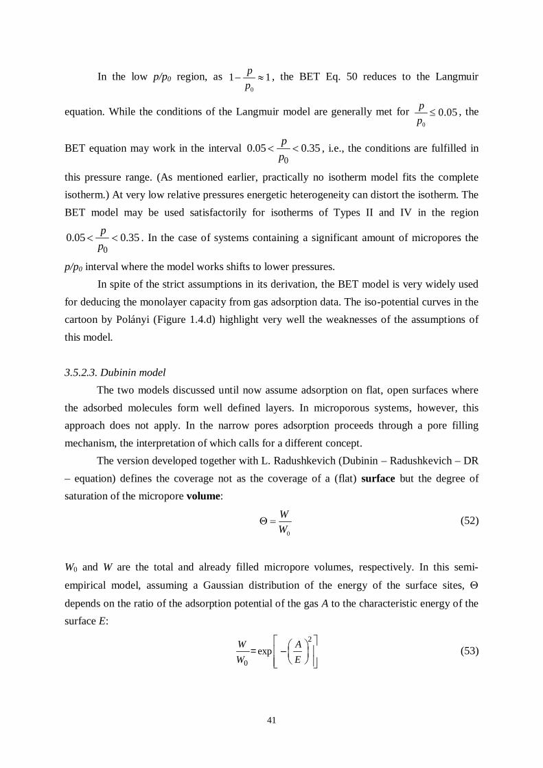
The two models discussed until now assume adsorption on flat, open surfaces where the adsorbed molecules form well defined layers. In microporous systems, however, this approach does not apply. In the narrow pores adsorption proceeds through a pore filling mechanism, the interpretation of which calls for a different concept.

The version developed together with L. Radushkevich (Dubinin – Radushkevich – DR – equation) defines the coverage not as the coverage of a (flat) surface but the degree of saturation of the micropore volume:

0

WW

(52)

W0 and W are the total and already filled micropore volumes, respectively. In this semi-

empirical model, assuming a Gaussian distribution of the energy of the surface sites,

depends on the ratio of the adsorption potential of the gas A to the characteristic energy of the surface E:

2

0exp

W AW E

= – (53)

42

According to Polány, the adsorption potential of the gas A is defined as

0ln pA RT

p

= – . (54)

i.e., the isothermal work to be supplied when the pressure of the gas is compressed from p to p0 in the adsorption space. Combining Eqs. 53 and 54, we obtain

2

0

0

lnexp

pRTW pW E

= – , (55)

This equation yields the macroscopic behaviour for adsorption loading at a given pressure. Its logarithmic expression is

22 0

0ln ln pW RT

W E p

= . (56)

If the DR model is valid, the measured data should fall on a straight line in a plot of lnW – ln2(p0/p) . From the fitting parameters of the linear plot the total volume of the micropores and the characteristic energy of the surface can be deduced (Figure 3.19.).

Figure 3.19. Linear DR plot: lnW – ln2(p0/p).

43

A successful fit with the model can be obtained in the low pressure region in

microporous materials, where adsorption takes place by pore filling (see Figures 14 and15).

Astakhov and Stöckli have developed an analogous formula for surfaces with non-Gaussian

energy distributions. Dubinin’s model equations are the most widely used to describe

adsorption in microporous materials, especially those of carbonaceous origin.

3.5.3. New models

The rapid development of computers has opened new avenues, allowing potential

models to expand the relative pressure range, and also in developing enhanced models that

describe adsorption processes. Non-linear density function theory (NLDFT) and/or Grand

Canonical Monte Carlo (GCMC) simulations make it possible to fit a so-called Generalized

Adsorption Isotherm (GAI) to a complete isotherm. Figure 3.20. illustrates the Monte Carlo

simulation of multilayer adsorption.

Figure 3.20. Monte Carlo simulation of multilayer adsorption.

The most frequently used isotherm models are summarized in Table 3.1.

44

Table 3.1. The most frequently used isotherm model equations.

Model Equation Reference

Henry sHn k p

Langmuir

s mn K pn

K p

1

Langmuir, L, J. Amer. Chem.

Soc. 38 (11): 2221–2295

(1916).

Langmuir, L, J. Amer. Chem.

Soc. 40 (9): 1361–1403

(1918).

Brunauer-Emmett-

Teller (BET)

0

0 0 0

1 1

ms

pn Cpn

p p pCp p p

, where

netQRTC e

Brunauer, S, Emmett, PH,

Teller E, J. Amer. Chem. Soc.

60 (2): 309–319 (1938).

Freundlich s / m'Fn k p 1 Freundlich, H, Colloid and

Capillary Chemistry,

Methuen, London 1926

Dubinin

0 expNAW W

E

= – , where

0

ln pA RTp

Polanyi, M, Verh. Dtsch.

Phys. Ges. 16:1012 (1914).

Dubinin, MM, Radushkevich,

LV, Dokl. Akad. Nauk. SSSR

55:331 (1947).

Dubinin MM, Astakhov VA,

Adv. Chem. Ser. 102: 69

(1970).

Stöckli, HF, Carbon 28 (1):1-

6 (1990).

Temkin smn n A' ln p B Lowell, S , Shields, JE,

Thomas, MA, Thommes, M,

Characterization of Porous

Solids and Powders: Surface

Area, Pore Size and Density,

45

Springer, Inc., Dordrecht

2006, p. 225

Tóth

1/

1

s mmm

n K pnK p

Toth, J, Acta Chim. Acad.

Sci. Hung. 69:329 (1971).

Horváth-Kawazoe

40 0

4 10 4 10

3 9 3 90 0 0 0

1 2

3 1 9 1 3 9

s s a aA N A N ANplnp RT ( d )

d d d d

=

Horváth, G, Kawazoe, K, J.

Chem. Eng. Japan 16, 474

(1983)

Generalized

Adsorption

Isotherm (GAI)

max

min

ws a

w

p pn n ,w f w d wp p

0 0

= Lowell, S , Shields, JE,

Thomas, MA, Thommes, M,

Characterization of Porous

Solids and Powders: Surface

Area, Pore Size and Density,

Springer, Inc., Dordrecht

2006, p. 33

46

3.6. Heat of adsorption

It was demonstrated earlier that adsorption is a spontaneous process (Chapter 1.1.)

and a great part of the evolving heat comes from the loss of mobility of the adsorptive. In the

case of a pure adsorptive the heat effect simultaneously characterizes the strength of the

interaction(s) and the heterogeneity of the surface site. The heat developed during the

adsorption may be expressed either in integral (Qint) or differential (Qdiff) form:

- Qint is the heat evolved when the total amount of gas adsorbs on unit mass of pure

adsorbent,

- Qdiff is the heat evolved when only a limited part of the gas adsorbs on the solid

surface. max

int0

m diffQ n Q d (57)

The latter depends on the coverage, since high energy sites will be occupied first.

Consequently the shape of ( ) diffQ f depends on the energy distribution of the surface

sites (Figure X). Isotherm models can assume a variety of distributions. According to the

concept of the Langmuir model all the surface sites are of equal energy, i.e., Qdiff is constant,

i.e., ( ) diffQ f . In the derivation of the Temkin model a linear distribution of the surface

site energy is assumed, while the Freundlich model assumes that the energy distribution

decreases exponentially (Table 3.1).

Figure 3.21. Qdiff generally decreases changes as adsorption progresses.

47

Both the differential and the integral heat of adsorption can be measured directly by

calorimetric methods. Information about the adsorption interaction however can also be

deduced from the adsorption isotherms. All three models discussed in detail in the previous

sessions contain a parameter that is related to this phenomenon.

In the Langmuir model according to Eq. (39) this parameter is the equilibrium

constant of the adsorption process. The change in Gibbs free energy of the process can be

obtained if Ktd is known, i.e., once K is converted to Ktd, G can be calculated. The relation

between the adsorption energy and the C parameter of the BET model (Eq. 50) was already

shown. From the slope of the logarithmic DR plot the characteristic energy of the surface can

be obtained (Figure 3.19).

As ( ) diffQ f , it is convenient to express Qdiff as an isosteric heat of adsorption

Qisost, i.e., at equal surface coverage for different temperatures. The isotherms must therefore

be measured at two different temperatures at least. From a ( ) f p plot (where p is the

equilibrium pressure) the corresponding p-T pairs can be determined at several values as

shown in Figure 3.22.

Figure 3.22. Determination of the p –T pairs for the calculation of Qisost.

The temperature dependence of the adsorption equilibrium constant can be found from

a van 't Hoff type equation6:

6 The differential form is 2ln , d K H

dT RT

= and the definite integral from T1 to T2 is 2

1 2 1

1 1ln K H

K R T T

=

48

2

ln =

isostQpT RT

(58)

From the corresponding plots of lnp – 1/T pairs, Qisost can be obtained as the slope of the plot

at each selected coverage (Figure 3.23.). A representation of the form of Figure 3.24 can be

obtained if the Qisost values are plotted against either the coverage or the adsorbed volume.

Once all the pores are filled Qisost becomes practically identical to the heat of condensation.

Figure 3.23. The slope of the straight line is Qisos.

Figure 3.24. The isosteric heat of adsorption depends on the coverage (the amount

already adsorbed). Qisost of water vapour on magnetite (Fe3O4) in the range 293 - 303K. (The

heat of condensation of water is 40.8 kJ/mol.).

49

3.7. Morphological characterisation of adsorbent from gas adsorption isotherms

3.7.1. Surface area

The (specific) surface area was already defined in Eq. (20). For particles of irregular

shape, porous materials, or small particles it is practically impossible to estimate it directly by

geometrical measurement. Monolayer coverage obtained from adsorption measurements

however is an excellent tool for determining the surface area of an adsorbent. In spite of its

imperfections, it is still the BET model that is most often used to derive the monolayer

capacity. IUPAC has issued best practice recommendations for experimental data collection.

According to these recommendations, the adsorptive is nitrogen gas and the

experiment is performed at its atmospheric boiling point (T = 77.35 K) using liquid nitrogen

as cooling medium. (Therefore p0 is determined by the actual barometric pressure.) As the

BET model generally works in the range 0.5 < p/p0 < 0.35, this section of the isotherm is

plotted in the linear form (Eq. 51). For microporous solids the linear range shifts to lower

pressures. Generally five equally distributed points in this pressure range are selected

(multipoint method). The monolayer capacity nm [mol N2/1 g solid sample] is derived from

the parameters of the straight line fit to the BET equation. Bear in mind that neither the slope

nor the intercept may be negative.

The advantage of nitrogen is that its interactions with surface sites are only secondary

and weak. It is therefore assumed that each molecule in the closely packed monolayer covers

an identical area of the solid surface. This cross sectional area as is 0.162 nm2/molecule. We

use Avogadro’s number to relate these numbers to macroscopic quantities. The (specific)

surface area is thus

s m A sA n N a (59)

The sensitivity of modern commercial gas adsorption instruments requires 0.5 - 1 m2

adsorbent surface area in the measuring cell for surface area determination. Typical surface

areas of adsorbents are listed in Table 3.2.

If the other parameter C of the BET equation is large enough (C 80) the intercept 1 0mn C

,

i.e., one point of the straight line is known and only one more point is needed to estimate the

monolayer capacity (single point method). This method is fast but certainly not necessarily

accurate. It is often used when a rapid estimate of the surface area is required (technology

50

control). The single point selected is generally p/p0 = 0.3 (c.f. the gas composition in the

dynamic method, Chapter 3.4.3.).

Table 3.2. Surface area of typical adsorbents.

material surface area, m2/g

activated carbon 600–1400

silica gel 300–600

catalyst 50–300

dust, particle size d = 0.1 mm 0.1–0.5

In certain cases the use of other gas probe molecules than nitrogen may be

advantageous. For materials with extremely low surface area, krypton gas can be used, as its

saturation pressure at the boiling point of nitrogen (normal boiling point 119.93 K), where the

measurements are generally performed, is low (Table 3.3.). For surfaces with outstandingly

polar character, the permanent quadrupole moment of nitrogen may be a drawback. In these

cases, argon is recommended (normal boiling point: 87.27 K), either at its own boiling point

or at 77 K.

Table 3.3. Temperature dependence of the saturation pressure of krypton gas.

T (K) 59 65 74 84 99 120

p(Pa) 1 10 100 1000 10.000 100.000

In the case of microporous materials the BET model overestimates the surface area

since all the molecules filling the micropores in the linear relative pressure range used for nm

calculation are assumed to be adsorbates directly in contact with the surface. The situation is

similar when the micropore volume W0 from the DR model is used to derive the surface area.

Table 3.4. lists the cross sectional area of the most common probe gases.

51

Table 3.4. Cross sectional area as of gas/vapour probes.

Gas or

vapour

Temperature,

°C

Molar mass as,

nm2/molecule

N2 –195 28.01 0.162

Ar –195 39.95 0.142

Kr –195 83.80 0.20

Xe –195 131.29 0.25

O2 –185 32.0 0.14

Ethane –195 30.07 0.21

Benzene 25 78.11 0.40

H2O(g) 25 18.02 0.125

CO2 0 44.01 0.17

t-method

Figure 3.16.a shows that the thickness of real adsorbed films is irregular. They are therefore

generally characterized by a t statistical thickness. This can be calculated from the number of

the layers and the thickness of a single complete layer d as

s

m

Vt dV

(60)

where Vs is the actual volume adsorbed and Vm is the volume belonging to the monolayer

thickness. For nitrogen d= 0.35 nm.

By means of Eq. 60 or semi-empyrical equations (e.g., Eq. 65) the isotherms 0( )sTV f p /p

can be converted to ( )sV f t plots. Figure 3.25 shows the original isotherm and the initial

sections of the corresponding t-plots. Figure 3.25.a represents a typically non-microporous

system: the adsorbed volume is directly proportional to the layer thickness and the slope of

the straight line gives the surface area. The intercept is 0 and the slope sdV

dt is equal to the

surface area of the system. It generally gives very good agreement with the surface area

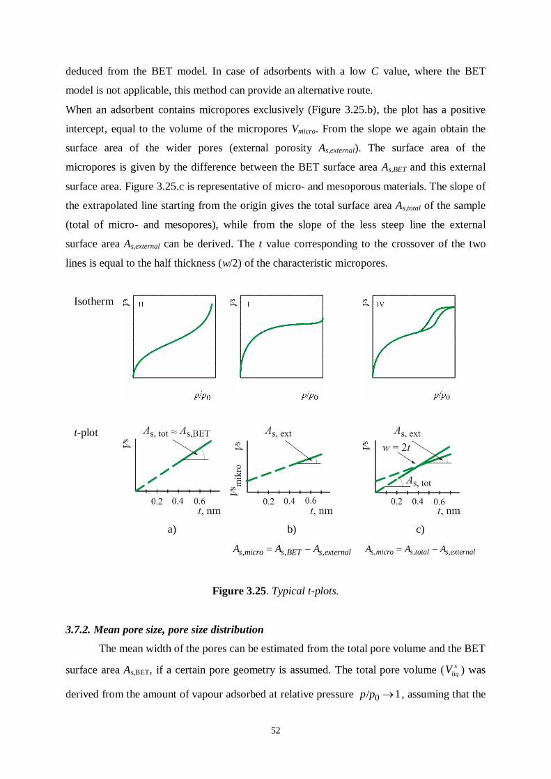
52

deduced from the BET model. In case of adsorbents with a low C value, where the BET

model is not applicable, this method can provide an alternative route.

When an adsorbent contains micropores exclusively (Figure 3.25.b), the plot has a positive

intercept, equal to the volume of the micropores Vmicro. From the slope we again obtain the

surface area of the wider pores (external porosity As,external). The surface area of the

micropores is given by the difference between the BET surface area As,BET and this external

surface area. Figure 3.25.c is representative of micro- and mesoporous materials. The slope of

the extrapolated line starting from the origin gives the total surface area As,total of the sample

(total of micro- and mesopores), while from the slope of the less steep line the external

surface area As,external can be derived. The t value corresponding to the crossover of the two

lines is equal to the half thickness (w/2) of the characteristic micropores.

Isotherm

t-plot

a) b) c)

, , , s micro s BET s externalA A A , , , s micro s total s externalA A A

Figure 3.25. Typical t-plots.

3.7.2. Mean pore size, pore size distribution

The mean width of the pores can be estimated from the total pore volume and the BET

surface area As,BET, if a certain pore geometry is assumed. The total pore volume ( sliqV ) was

derived from the amount of vapour adsorbed at relative pressure 0/ 1p p , assuming that the

53

pores are then filled with liquid adsorbate. In the case of open ended cylindrical pores the

radius rp can be calculated as

,

2 sliq

ps BET

Vr

A (61)

For slit shaped pores of parallel walls the mean pore width is w is given as

,

2 sliq

s BET

Vw

A (62)

Since the vapour pressure over a curved surface is higher than over a flat one, vapours

condense into narrow capillaries at vapour pressures lower than their saturation pressure. The

pore size distribution (PSD) can be obtained from the Kelvin7 equation, which describes the

change in vapour pressure due to a curved liquid/vapour interface with radius rK:

0

2 cosln L

K

Vpp r R T

= - (63)

is the surface tension, VL is the molar volume of the adsorbate in liquid form, is the

contact angle of the adsorbate on the pore wall and rK is the so called Kelvin radius of the

cylindrical pore. Complete wetting is assumed, i.e., cos = 1. The equation relates the radius

of the pores rK to the relative pressure p/p0. With the Kelvin equation the function

( )sTV f p can easily be rescaled to the form ( )s

KV f r . All pores no wider than rK are

filled with liquid adsorbate at the corresponding p/p0. If the corresponding values are 1sV at

rK,1 and 2sV at rK,2, the volume of the liquid gas filling the pores in the (rK,2 - rK,1) range can be

deduced from 2 1s sV V (here we assumed that rK,2 rK,1 ). The Kelvin equation can be used

in the mesopore range (2-50 nm). For wider pores the results are unreliable due to the

exponential nature of the relationship. 7 William Thomson (1824 – 1907) was an Irish and British mathematical physicist and engineer. (For his work on the transatlantic telegraph project he was knighted by Queen Victoria, becoming Sir William Thomson.) He also determined the correct value of absolute zero (approximately -273.15 Celsius). The unit of absolute or thermodynamic temperature is called kelvin in his honour.

54

Later we show (Figure 3.28.) that the real size of the pore is wider than rK, as a layer

of thickness t remains on the solid after desorption. The real radius of the pore is thus

Kr r t . (64)

t can be also estimated from semi-empirical equations, such as

3 0

50.35 , nmln

t pp

= (65)

for N2 molecules at 77 K.

The adsorption hysteresis

In the case of mesoporous adsorbents, adsorption is typically irreversible and thus the

adsorption and desorption branches do not overlap. A reproducible hysteresis loop appears in

the range 0/ 0.42p p . The reason for this phenomenon is that either in the adsorption or in

the desorption measurement the adsorbate is in a metastable state. Note that the desorption

branch always lies above that of adsorption. According to the IUPAC classification, isotherms

of Type IV and V typically possess such a hysteresis loop (Figure 3.10.).

Figure 3.26. shows a few characteristic pore shapes. We recall that pores may also

form in the spaces between (non)porous particles (Figure 2.7.)

Figure 3.26. Typical pore shapes.

The hysteresis loops are also classified (Figure 3.27). The shape of the loop may help

to decide which loop to use to deduce the pore size distribution: in the case of type H1 the

desorption, ill all the other cases the desorption branch is recommended.

55

Figure 3.27. IUPAC classification of the hysteresis loops. H1: open ended cylindrical

pores with narrow size distribution; H2: network of pores with different shape and size; H3:

slit shaped pores formed in lamellar solids; H4: pore shape similar to H3, but the adsorbent

is highly microporous.

The source of hysteresis:

i) different mechanisms in the processes of adsorption and desorption;

ii) delayed/hindered desorption (irregular pore shape, variation of the pore size along

the pore, networking)

The different mechanism in the case of cylindrical pores is illustrated in Figure 3.28.

Adsorption layers form along the walls of the cylinder until the whole cylinder is filled with

the liquid adsorbate and a meniscus is formed. The desorption will start from this curved

meniscus.

Figure 3.28. The mechanism of the adsorption and desorption are different.

56

The thermodynamic explanation for this example is as follows. The change of the

Gibbs free energy G during the adsorption is

0ln pdG dn RT dn

p

= = (66)

The change of the Gibbs free energy G’ when the S/L interface is formed can be written as

' SL SG sdG dA = – (67)

where is the surface tension of the interfaces developing between the solid/liquid and

solid/gas phases respectively, as labelled in the indices. The difference can be expressed by

the surface tension between the liquid and the gas phases LG using Young’s equation8

' ( cos )SL SG s LG sdG dA dA = – – (68b)

At equilibrium

'dG dG= (69)

0ln cosLG s

pRT dn dAp

= – (70)

m

dVdnV

= (71)

Vm is the molar volume of the adsorbate in liquid state

0ln cosLG s

m

p dVRT dAp V

= – . (72)

If the liquid adsorbent wets9 the solid surface completely, the contact angle is 0, and cos = 1.

Thus 8 cosSG SL LG = , is the contact angle between the solid and liquid phases

57

0ln

m LG

s

VdVdA pRT

p

= – . (73)

We will consider the influence of the two mechanisms for cylindrical pores providing H1 type

hysteresis loopes. During the adsorption on the wall of the cylindrical pore of length l and

radius r, the volume V and the surface of the wall As can be expressed respectively as

2V r l= (74)

and

2sA r l= (75)

During the process the radius of the cylinder decreases continuously. Therefore

2dV rldr=– (76)

and

2sdA ldr= – (77)

Thus

s

dV rdA

= . (78)

should be substituted into Eq. 73. The result is the Kelvin equation given in Eq. 63

(remember, cos = 1).

In the desorption cycle the meniscus can be taken to be a hemisphere of radius r.

34

3 2rV

= (79)

242s

rA = (80)

4sdA rdr= (81)

9 see http://en.wikipedia.org/wiki/Wetting

58

2212 2

6r drdV r dr

= (82)

Thus the left-hand side of Eq. 73 is

2s

dV rdA

= . (83)

That is, two different radii correspond to the same relative pressure, i.e., when we

rescale the p/p0 axis of the isotherms, the scaling function is different in the desorption

branch.

For the adsorption branch:

0

VmrRTp e

p

–= , (84)

and for the desorption

2

0

VmrRTp e

p

–= . (85)

Thus

2

0 0

a dp pp p

= . (86)

where the indices a and d mean adsorption and desorption.

The substantial difference between the two expressions also highlights the significance

of the choice of pore geometry in pore size distribution calculations.

Pore size distribution in the micropore range can be obtained by semi-empirical

equations, e.g., the equations of Horváth and Kawazoe (HK), of Saito and Foley (SF), of

Cheng and Yang or by the novel computational methods, e.g., non-linear density function

theory (NLDFT) or Grand Canonic Monte Carlo (GCMC) equations. The low end of the

distribution curves is limited by the size of the probe molecule.

Figure 3.29. compares the typical ranges of the experimental techniques applicable for

pores of various size. It is clear that the potential of gas adsorption is limited to pores

preferably not exceeding 50 nm (upper limit of mesoporosity).

59

Figure 3.29. Various methods for the determination of pore size distribution.

3.8. References

1. S Lowell, JE Shields. MA Thomas, M Thommes: Characterization of Porous Solids and

Powders: Surface Area, Pore Size and Density. Springer, 2006

2. SJ Gregg, KSW Sing: Adsorption, Surface Area and Porosity. Academic Press, 1982

3. F Rouquerol, J Rouquerol, K Sing: Adsorption by Powders and Porous Solids. Academic

Press, 1999

4. G Somorjay: Introduction to Surface Chemistry and Catalysis. Wiley, 1994