physically based deformable models in computer...
TRANSCRIPT

EUROGRAPHICS 2005 STAR – State of The Art Report
Physically Based Deformable Models in Computer Graphics
Andrew Nealen1, Matthias Müller2,3, Richard Keiser3, Eddy Boxerman4 and Mark Carlson5
1 Discrete Geometric Modeling Group, TU Darmstadt2 NovodeX / AGEIA
3 Computer Graphics Lab, ETH Zürich4 Department of Computer Science, University of British Columbia
5 DNA Productions, Inc.
AbstractPhysically based deformable models have been widely embraced by the Computer Graphics community. Manyproblems outlined in a previous survey by Gibson and Mirtich [GM97] have been addressed, thereby makingthese models interesting and useful for both offline and real-time applications, such as motion pictures and videogames. In this paper, we present the most significant contributions of the past decade, which produce such impres-sive and perceivably realistic animations and simulations: finite element/difference/volume methods, mass-springsystems, meshfree methods, coupled particle systems and reduced deformable models based on modal analysis.For completeness, we also make a connection to the simulation of other continua, such as fluids, gases and meltingobjects. Since time integration is inherent to all simulated phenomena, the general notion of time discretizationis treated separately, while specifics are left to the respective models. Finally, we discuss areas of application,such as elastoplastic deformation and fracture, cloth and hair animation, virtual surgery simulation, interactiveentertainment and fluid/smoke animation, and also suggest areas for future research.
Categories and Subject Descriptors(according to ACM CCS): I.3.5 [Computer Graphics]: Physically Based Model-ing I.3.7 [Computer Graphics]: Animation and Virtual Reality
1. Introduction
Physically based deformable models have two decades ofhistory in Computer Graphics: since Lasseter’s discussionof squash and stretch[Las87] and, concurrently, Terzopou-los et. al’s seminal paper on elastically deformable mod-els [TPBF87], numerous researchers have partaken in thequest for the visually and physically plausible animation ofdeformable objects and fluids. This inherently interdiscipli-nary field elegantly combines newtonian dynamics, contin-uum mechanics, numerical computation, differential geom-etry, vector calculus, approximation theory and ComputerGraphics (to name a few) into a vast and powerful toolkit,which is being further explored and extended. The field is inconstant flux and, thus, active and fruitful, with many visu-ally stunning achievements to account for.
Since Gibson and Mirtich’s survey paper [GM97], thefield of physically based deformable models in ComputerGraphics has expanded tremendously. Significant contribu-tions were made in many key areas, e.g. object model-
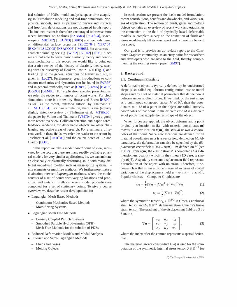
Figure 1: Hooke’s Law, fromDe Potentia Restitutiva [1678].
ing, fracture, plasticity, cloth animation, stable fluid simu-lation, time integration strategies, discretization and numer-
c© The Eurographics Association 2005.
Nealen, Müller, Keiser, Boxerman and Carlson / Physically Based Deformable Models in Computer Graphics
ical solution of PDEs, modal analysis, space-time adaptiv-ity, multiresolution modeling and real-time simulation. Non-physical models, such as parametric curves and surfacesand free-form deformations, are not discussed in this report.The inclined reader is therefore encouraged to browse morerecent literature on t-splines [SZBN03] [SCF∗04], space-warping [MJBF02] [LKG∗03] [BK05] and methods basedon differential surface properties [SLCO∗04] [YZX∗04][BK04] [LSLCO05] [NSACO05] [ IMH05]. For advances incharacter skinning see e.g. [WP02] [KJP02] [JT05]. Sincewe are not able to cover basic elasticity theory and contin-uum mechanics in this report, we would like to point outthat a nice review of the history of elasticity theory, start-ing with the discovery of Hooke’s Law in 1660 (Fig.1) andleading up to the general equations of Navier in 1821, isgiven in [Lov27]. Furthermore, great introductions to con-tinuum mechanics and dynamics can be found in [WB97]and in general textbooks, such as [Chu96] [Coo95] [BW97][Gdo93] [BLM00]. For application specific presentations,we refer the reader to a number of recent works. For clothsimulation, there is the text by House and Breen [HB00],as well as the recent, extensive tutorial by Thalmann etal. [MTCK∗04]. For hair simulation, there is the (alreadyslightly dated) overview by Thalmann et al. [MTHK00];the paper by Volino and Thalmann [VMT04] gives a good,more recent overview. Collision detection and haptic force-feedback rendering for deformable objects are other chal-lenging and active areas of research. For a summary of re-cent work in these fields, we refer the reader to the report byTeschner et al. [TKH∗05] and the course notes of Lin andOtaduy [LO05].
In this report we take amodel basedpoint of view, moti-vated by the fact that there are many readily available physi-cal models for very similar applications, i.e. we can animatean elastically or plastically deforming solid with many dif-ferent underlying models, such as mass-spring systems, fi-nite elements or meshfree methods. We furthermore make adistinction betweenLagrangianmethods, where the modelconsists of a set of points with varying locations and prop-erties, andEulerian methods, where model properties arecomputed for a set of stationary points. To give a coarseoverview, we describe recent developments for
• Lagrangian Mesh Based Methods
– Continuum Mechanics Based Methods– Mass-Spring Systems
• Lagrangian Mesh Free Methods
– Loosely Coupled Particle Systems– Smoothed Particle Hydrodynamics (SPH)– Mesh Free Methods for the solution of PDEs
• Reduced Deformation Models and Modal Analysis• Eulerian and Semi-Lagrangian Methods
– Fluids and Gases– Melting Objects
In each section we present the basic model formulation,recent contributions, benefits and drawbacks, and various ar-eas of application. The section on fluids, gases and meltingobjects contains an overview of recent work and establishesthe connection to the field of physically based deformablemodels. A complete survey on the animation of fluids andgases would easily fill its own report and is therefore beyondour scope.
Our goal is to provide an up-to-date report to the Com-puter Graphics community, as an entry point for researchersand developers who are new to the field, thereby comple-menting the existing survey paper [GM97].
2. Background
2.1. Continuum Elasticity
A deformable object is typically defined by its undeformedshape (also called equilibrium configuration, rest or initialshape) and by a set of material parameters that define how itdeforms under applied forces. If we think of the rest shapeas a continuous connected subsetM of R
3, then the coor-dinatesm ∈ M of a point in the object are calledmaterialcoordinatesof that point. In the discrete caseM is a discreteset of points that sample the rest shape of the object.
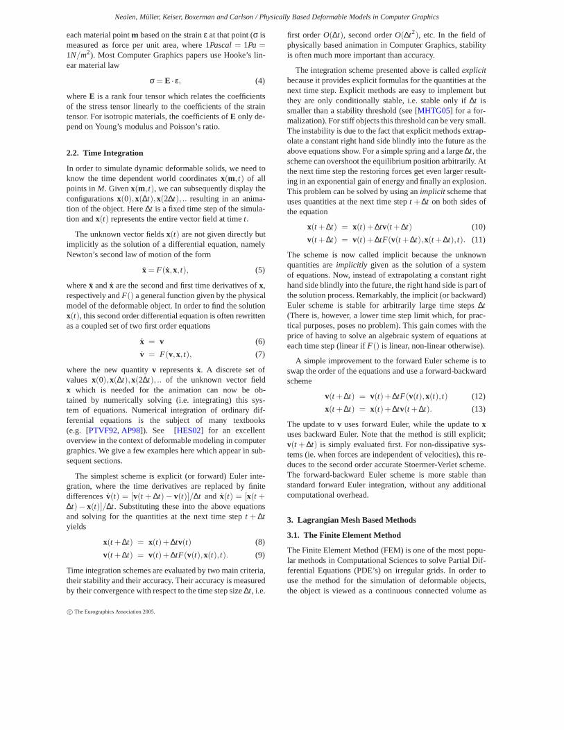
When forces are applied, the object deforms and a pointoriginally at locationm (i.e. with material coordinatesm)moves to a new locationx(m), thespatial or world coordi-natesof that point. Since new locations are defined for allmaterial coordinatesm, x is a vector field defined onM. Al-ternatively, the deformation can also be specified by thedis-placementvector fieldu(m) = x(m)−m defined onM (seeFig. 2). Fromu(m) the elastic strainε is computed (ε is a di-mensionless quantity which, in the (linear) 1D case, is sim-ply ∆l/l ). A spatially constant displacement field representsa translation of the object with no strain. Therefore, it be-comes clear that strain must be measured in terms of spatialvariations of the displacement fieldu = u(m) = (u,v,w)T .Popular choices in Computer Graphics are
εG =12(∇u +[∇u]T +[∇u]T∇u) (1)
εC =12(∇u +[∇u]T), (2)
where the symmetric tensorεG ∈ R3x3 is Green’s nonlinear
strain tensor andεC ∈ R3x3 its linearization, Cauchy’s linear
strain tensor. The gradient of the displacement field is a 3 by3 matrix
∇u =
u,x u,y u,z
v,x v,y v,z
w,x w,y w,z
, (3)
where the index after the comma represents a spatial deriva-tive.
The material law (orconstitutive law) is used for the com-putation of the symmetric internal stress tensorσ ∈ R
3x3 for
c© The Eurographics Association 2005.
Nealen, Müller, Keiser, Boxerman and Carlson / Physically Based Deformable Models in Computer Graphics
each material pointm based on the strainε at that point (σ ismeasured as force per unit area, where 1Pascal= 1Pa =1N/m2). Most Computer Graphics papers use Hooke’s lin-ear material law
σ = E · ε, (4)
whereE is a rank four tensor which relates the coefficientsof the stress tensor linearly to the coefficients of the straintensor. For isotropic materials, the coefficients ofE only de-pend on Young’s modulus and Poisson’s ratio.
2.2. Time Integration
In order to simulate dynamic deformable solids, we need toknow the time dependent world coordinatesx(m, t) of allpoints inM. Givenx(m, t), we can subsequently display theconfigurationsx(0),x(∆t),x(2∆t), .. resulting in an anima-tion of the object. Here∆t is a fixed time step of the simula-tion andx(t) represents the entire vector field at timet.
The unknown vector fieldsx(t) are not given directly butimplicitly as the solution of a differential equation, namelyNewton’s second law of motion of the form
x = F(x,x, t), (5)
wherex andx are the second and first time derivatives ofx,respectively andF() a general function given by the physicalmodel of the deformable object. In order to find the solutionx(t), this second order differential equation is often rewrittenas a coupled set of two first order equations
x = v (6)
v = F(v,x, t), (7)
where the new quantityv representsx. A discrete set ofvalues x(0),x(∆t),x(2∆t), .. of the unknown vector fieldx which is needed for the animation can now be ob-tained by numerically solving (i.e. integrating) this sys-tem of equations. Numerical integration of ordinary dif-ferential equations is the subject of many textbooks(e.g. [PTVF92, AP98]). See [HES02] for an excellentoverview in the context of deformable modeling in computergraphics. We give a few examples here which appear in sub-sequent sections.
The simplest scheme is explicit (or forward) Euler inte-gration, where the time derivatives are replaced by finitedifferencesv(t) = [v(t + ∆t)− v(t)]/∆t and x(t) = [x(t +∆t)− x(t)]/∆t. Substituting these into the above equationsand solving for the quantities at the next time stept + ∆tyields
x(t +∆t) = x(t)+∆tv(t) (8)
v(t +∆t) = v(t)+∆tF(v(t),x(t), t). (9)
Time integration schemes are evaluated by two main criteria,their stability and their accuracy. Their accuracy is measuredby their convergence with respect to the time step size∆t, i.e.
first orderO(∆t), second orderO(∆t2), etc. In the field ofphysically based animation in Computer Graphics, stabilityis often much more important than accuracy.
The integration scheme presented above is calledexplicitbecause it provides explicit formulas for the quantities at thenext time step. Explicit methods are easy to implement butthey are only conditionally stable, i.e. stable only if∆t issmaller than a stability threshold (see [MHTG05] for a for-malization). For stiff objects this threshold can be very small.The instability is due to the fact that explicit methods extrap-olate a constant right hand side blindly into the future as theabove equations show. For a simple spring and a large∆t, thescheme can overshoot the equilibrium position arbitrarily. Atthe next time step the restoring forces get even larger result-ing in an exponential gain of energy and finally an explosion.This problem can be solved by using animplicit scheme thatuses quantities at the next time stept + ∆t on both sides ofthe equation
x(t +∆t) = x(t)+∆tv(t +∆t) (10)
v(t +∆t) = v(t)+∆tF(v(t +∆t),x(t +∆t), t). (11)
The scheme is now called implicit because the unknownquantities areimplicitly given as the solution of a systemof equations. Now, instead of extrapolating a constant righthand side blindly into the future, the right hand side is part ofthe solution process. Remarkably, the implicit (or backward)Euler scheme is stable for arbitrarily large time steps∆t(There is, however, a lower time step limit which, for prac-tical purposes, poses no problem). This gain comes with theprice of having to solve an algebraic system of equations ateach time step (linear ifF() is linear, non-linear otherwise).
A simple improvement to the forward Euler scheme is toswap the order of the equations and use a forward-backwardscheme
v(t +∆t) = v(t)+∆tF(v(t),x(t), t) (12)
x(t +∆t) = x(t)+∆tv(t +∆t). (13)
The update tov uses forward Euler, while the update toxuses backward Euler. Note that the method is still explicit;v(t + ∆t) is simply evaluated first. For non-dissipative sys-tems (ie. when forces are independent of velocities), this re-duces to the second order accurate Stoermer-Verlet scheme.The forward-backward Euler scheme is more stable thanstandard forward Euler integration, without any additionalcomputational overhead.
3. Lagrangian Mesh Based Methods
3.1. The Finite Element Method
The Finite Element Method (FEM) is one of the most popu-lar methods in Computational Sciences to solve Partial Dif-ferential Equations (PDE’s) on irregular grids. In order touse the method for the simulation of deformable objects,the object is viewed as a continuous connected volume as
c© The Eurographics Association 2005.
Nealen, Müller, Keiser, Boxerman and Carlson / Physically Based Deformable Models in Computer Graphics
u(m)
(a)
m
x(m)
m
(b)
)(~ mu
)(~ mx
im
ix
Figure 2: In the Finite Element method, a continuous defor-mation (a) is approximated by a sum of (linear) basis func-tions defined inside a set of finite elements (b).
in Section2.1 which is discretized using an irregular mesh.Continuum mechanics, then, provides the PDE to be solved.
The PDE governing dynamic elastic materials is given by
ρx = ∇·σ+ f, (14)
whereρ is the density of the material andf externally appliedforces such as gravity or collision forces. The divergence op-erator turns the 3 by 3 stress tensor back into a 3 vector
∇·σ =
σxx,x +σxy,y +σxz,z
σyx,x +σyy,y +σyz,z
σzx,x +σzy,y +σzz,z
, (15)
representing the internal force resulting from a deformed in-finitesimal volume. Eq.14 shows the equation of motion indifferential form in contrast to theintegral form which isused in the Finite Volume method.
The Finite Element Method is used to turn a PDE into aset of algebraic equations which are then solved numerically.To this end, the domainM is discretized into a finite numberof disjoint elements (i.e. a mesh). Instead of solving for thespatially continuous functionx(m, t), one only solves for thediscrete set of unknown positionsxi(t) of the nodes of themesh. First, the functionx(m, t) is approximated using thenodal values by
x(m, t) = ∑i
xi(t)bi(m), (16)
wherebi() are fixed nodal basis functions which are 1 atnode i and zero at all other nodes, also known as the Kro-necker Delta property (see Fig.2). In the most general caseof the Finite Element Method, the basis functions do nothave this property. In that case, the unknowns are general pa-rameters which can not be interpreted as nodal values. Sub-stituting x(m, t) into Eq. 14 results in algebraic equationsfor thexi(t). In the Galerkin approach [Hun05], finding theunknownsxi(t) is viewed as an optimization process. Whensubstitutingx(m, t) by the approximationx(m, t), the infi-nitely dimensional search space of possible solutions is re-duced to a finite dimensional subspace. In general, no func-tion in that subspace can solve the original PDE. The approx-imation will generate a deviation or residue when substituted
into the PDE. In the Galerkin method, the approximationwhich minimizes the residueis sought. In other words, welook for an approximation whose residue is perpendicular tothe subspace of functions defined by Eq.16.
Many papers in Computer Graphics use a simple formof the Finite Element method for the simulation of de-formable objects, sometimes called theexplicit Finite Ele-ment Method, which is quite easy to understand and to im-plement (e.g. [OH99], [DDCB01], [MDM∗02]). The explicitFinite Element Method is not to be confused with the stan-dard Finite Element Method beingintegratedexplicitly. Theexplicit Finite Element Method can be integrated either ex-plicitly or implicitly.
In the explicit Finite Element approach, both, the massesand the internal and external forces are lumped to the ver-tices. The nodes in the mesh are treated like mass points in amass-spring system while each element acts like a general-ized spring connecting all adjacent mass points. The forcesacting on the nodes of an element due to its deformationare computed as follows (see for instance [OH99]): giventhe positions of the vertices of an element and the fixed ba-sis functions, the continuous deformation fieldu(m) insidethe element can be computed using Eq.16. Fromu(m), thestrain fieldε(m) and stress fieldσ(m) are computed. Thedeformation energy of the element is then given by
E =�
Vε(m) ·σ(m)dm, (17)
where the dot represents the componentwise scalar prod-uct of the two tensors. The forces can then be computed asthe derivatives of the energy with respect to the nodal posi-tions. In general, the relationship between nodal forces andnodal positions is nonlinear. When linearized, the relation-ship for an elemente connectingne nodes can simply beexpressed as
fe = Keue, (18)
wherefe ∈ R3ne contains thene nodal forces andue ∈ R
3ne
thene nodal displacements of an element. The matrixKe ∈R
3nex3ne is called thestiffness matrixof the element. Becauseelastic forces coming from adjacent elements add up at anode, a stiffness matrixK ∈ R
3nx3n for an enire mesh withn nodes can be formed by assembling the element’s stiffnessmatrices
K = ∑e
Ke. (19)
In this sum, the element’s stiffness matrices are expanded tothe dimension ofK by filling in zeros at positions relatedto nodes not adjacent to the element. Using the linearizedelastic forces, the linear algebraic equation of motion for anentire mesh becomes (u = x− x0)
Mu+Du+Ku = fext, (20)
whereM ∈ Rnxn is the mass matrix,D ∈ R
nxn the damping
c© The Eurographics Association 2005.
Nealen, Müller, Keiser, Boxerman and Carlson / Physically Based Deformable Models in Computer Graphics
matrix andfext ∈ Rn externally applied forces. Often, diago-
nal matrices are used forM andD, a technique calledmasslumping. In this case,M just contains the point masses ofthe nodes of the mesh on its diagonal. The vectorsx andx0contain, respectively, the actual and the rest positions of thenodes.
The Finite Element method only produces alinear sys-tem of algebraic equations if applied to alinear PDE. If alinear strain measure is used and Hooke’s law for isotropicmaterials is substituted into14, Lamé’s linear PDE results:
ρx = µ∆u +(λ +µ)∇(∇·u), (21)
where the material constantsλ andµ can be computed di-rectly from Young’s modulus and Poisson’s ratio. This equa-tion is solved in [DDBC99] in a multiresolution fashion.Using discretized versions of the Laplacian (∆ = ∇2) andgradient-of-divergence (∇(∇·)) operators, they solve theLamé equation on an irregular, multiresolution grid. Thesystem is optimized for limited deformations (linearizedstrain) and does not support topological changes. Based onGauss’ Divergence Theorem, the discrete operators are fur-ther evolved in [DDCB00], which leads to greater accuracythrough defined error bounds. Furthermore, the cubic octreehierarchy employed in [DDBC99] is succeeded by a non-nested hierarchy of meshes, in conformance with the rede-fined operators, which leads to improved shape sampling.In [DDCB01] the previous linearized physical model is re-placed by local explicit finite elements and Green’s nonlin-ear strain tensor. To increase stability the simulation is inte-grated semi-implicitly in time [DSB99].
O’Brien et al. [OH99] and [OBH02] present a FEM basedtechnique for simulating brittle and ductile fracture in con-nection with elastoplastic materials. They use tetrahedralmeshes in connection with linear basis functionsbi() andGreen’s strain tensor. The resulting nonlinear equations aresolved explicitly and integrated explicitly. The method pro-duces realistic and visually convincing results, but it is notdesigned for interactive or real-time use. In addition to thestrain tensor, they use the so-calledstrain rate tensor(thetime derivative of the strain tensor), to compute dampingforces. Other studies on the visual simulation of brittle frac-ture are [SWB00] and [MMDJ01].
Bro-Nielsen and Cotin [BNC96] use linearized finite el-ements for surgery simulation. They achieve significantspeedup by simulating only the visible surface nodes (con-densation), similar to the BEM. Many other studies suc-cessfully apply the FEM to surgery simulation, such as(but surely not limited to) [GTT89], [CEO∗93], [SBMH94],[KGC∗96], [CDA99], [CDA00], [PDA00] and [PDA01].
As long as the equation of motion is integrated explic-itly in time, nonlinear elastic forces resulting from Green’sstrain tensor pose no computational problems. The nonlin-ear formulas for the forces are simply evaluated and used di-rectly to integrate velocities and positions as in [OH99]. As
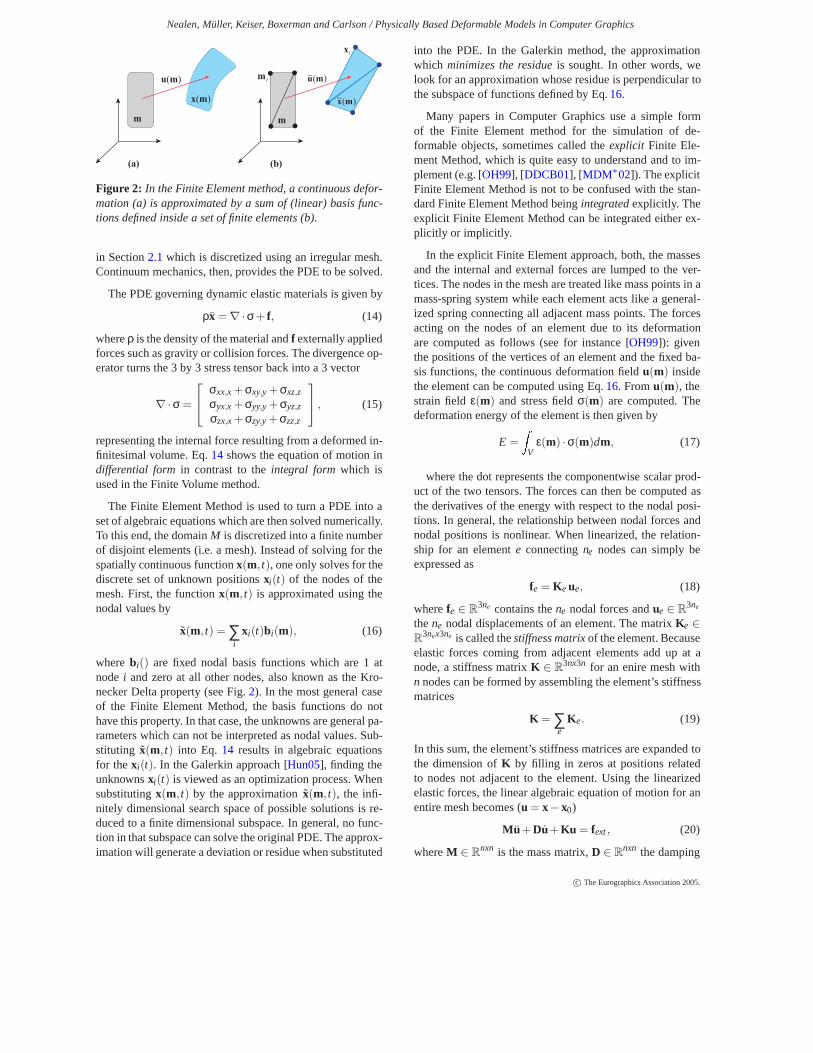
Figure 3: The pitbull with its inflated head (left) shows theartifact of linear FEM under large rotational deformations.The correct deformation is shown on the right.
mentioned earlier (Section2.2), explicit integration schemesare stable only for small time steps while implicit integra-tion schemes allow arbitrarily large time steps. However, inthe latter case, a system of algebraic equations needs to besolved at every time step. Linear PDE’s yield linear alge-braic systems which can be solved more efficiently and morestably than nonlinear ones. Unfortunately, linearized elasticforces are only valid for small deformations. Large rotationaldeformations yield highly inaccurate restoring forces (seeFig. 3).
To eliminate these artifacts, Müller et al. extract the ro-tational part of the deformation for each finite element andcompute the forces with respect to the non-rotated referenceframe [MG04]. The linear equation18 for the elastic forcesof an element (in this case a tetrahedron) is replaced by
f = RK (RTx− x0), (22)
whereR ∈ R12x12 is a matrix that contains four 3 by 3 iden-
tical rotation matrices along its diagonal. The vectorx con-tains the actual positions of the four adjacent nodes of thetetrahedron whilex0 contains their rest positions. The rota-tion of the element used inR is computed by performing apolar decomposition of the matrix that describes the trans-formation of the tetrahedron from the configurationx0 to theconfigurationx. This yields stable, fast and visually pleas-ing results. In an earlier approach, they extract the rotationalpart not per element but per node [MDM∗02]. In this case,the global stiffness matrix does not need to be reassembledat each time step but ghost forces are introduced.
Another solution to this problem is proposedin [CGC∗02]: each region of the finite element meshis associated with the bone of a simple skeleton and thenlocally linearized. The regions are blended in each timestep, leading to results which are visually indistinguishablefrom the nonlinear solution, yet much faster.
An adaptive nonlinear FEM simulation is described byWu et al. [WDGT01]. Distance, surface and volume preser-vation for triangular and tetrahedral meshes is outlinedin [THMG04]. Grinspun et al. introduce conforming, hierar-chical, adaptive refinement methods (CHARMS) for generalfinite elements [GKS02], refining basis functions instead ofelements. Irving et al. [ITF04] present a method which ro-bustly handles large deformation and element inversion by
c© The Eurographics Association 2005.
Nealen, Müller, Keiser, Boxerman and Carlson / Physically Based Deformable Models in Computer Graphics
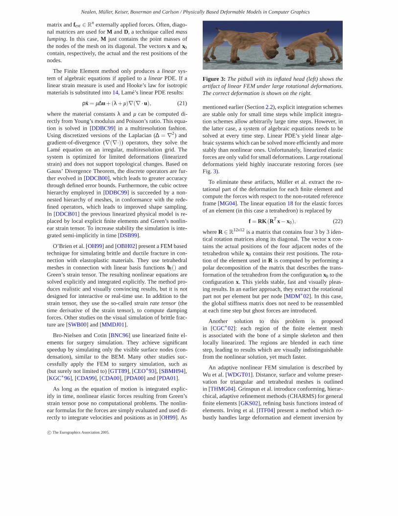
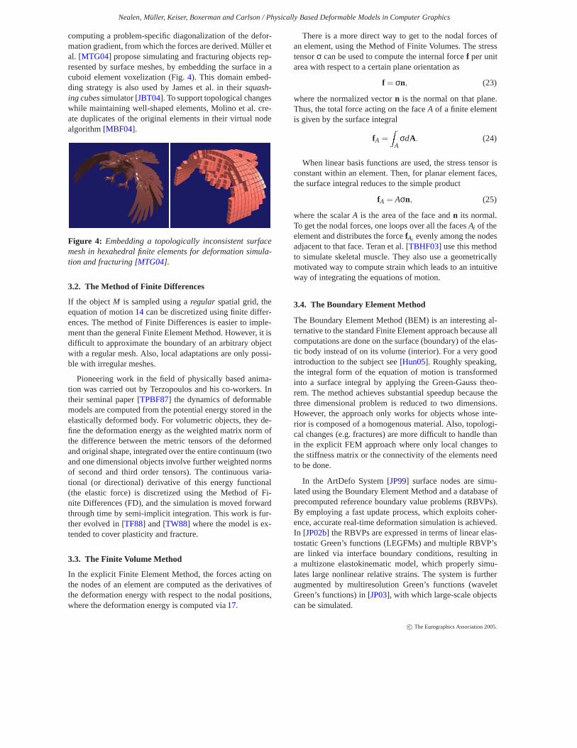
computing a problem-specific diagonalization of the defor-mation gradient, from which the forces are derived. Müller etal. [MTG04] propose simulating and fracturing objects rep-resented by surface meshes, by embedding the surface in acuboid element voxelization (Fig.4). This domain embed-ding strategy is also used by James et al. in theirsquash-ing cubessimulator [JBT04]. To support topological changeswhile maintaining well-shaped elements, Molino et al. cre-ate duplicates of the original elements in their virtual nodealgorithm [MBF04].
Figure 4: Embedding a topologically inconsistent surfacemesh in hexahedral finite elements for deformation simula-tion and fracturing [MTG04].
3.2. The Method of Finite Differences
If the objectM is sampled using aregular spatial grid, theequation of motion14 can be discretized using finite differ-ences. The method of Finite Differences is easier to imple-ment than the general Finite Element Method. However, it isdifficult to approximate the boundary of an arbitrary objectwith a regular mesh. Also, local adaptations are only possi-ble with irregular meshes.
Pioneering work in the field of physically based anima-tion was carried out by Terzopoulos and his co-workers. Intheir seminal paper [TPBF87] the dynamics of deformablemodels are computed from the potential energy stored in theelastically deformed body. For volumetric objects, they de-fine the deformation energy as the weighted matrix norm ofthe difference between the metric tensors of the deformedand original shape, integrated over the entire continuum (twoand one dimensional objects involve further weighted normsof second and third order tensors). The continuous varia-tional (or directional) derivative of this energy functional(the elastic force) is discretized using the Method of Fi-nite Differences (FD), and the simulation is moved forwardthrough time by semi-implicit integration. This work is fur-ther evolved in [TF88] and [TW88] where the model is ex-tended to cover plasticity and fracture.
3.3. The Finite Volume Method
In the explicit Finite Element Method, the forces acting onthe nodes of an element are computed as the derivatives ofthe deformation energy with respect to the nodal positions,where the deformation energy is computed via17.
There is a more direct way to get to the nodal forces ofan element, using the Method of Finite Volumes. The stresstensorσ can be used to compute the internal forcef per unitarea with respect to a certain plane orientation as
f = σn, (23)
where the normalized vectorn is the normal on that plane.Thus, the total force acting on the faceA of a finite elementis given by the surface integral
fA =�
AσdA. (24)
When linear basis functions are used, the stress tensor isconstant within an element. Then, for planar element faces,the surface integral reduces to the simple product
fA = Aσn, (25)
where the scalarA is the area of the face andn its normal.To get the nodal forces, one loops over all the facesAi of theelement and distributes the forcefAi evenly among the nodesadjacent to that face. Teran et al. [TBHF03] use this methodto simulate skeletal muscle. They also use a geometricallymotivated way to compute strain which leads to an intuitiveway of integrating the equations of motion.
3.4. The Boundary Element Method
The Boundary Element Method (BEM) is an interesting al-ternative to the standard Finite Element approach because allcomputations are done on the surface (boundary) of the elas-tic body instead of on its volume (interior). For a very goodintroduction to the subject see [Hun05]. Roughly speaking,the integral form of the equation of motion is transformedinto a surface integral by applying the Green-Gauss theo-rem. The method achieves substantial speedup because thethree dimensional problem is reduced to two dimensions.However, the approach only works for objects whose inte-rior is composed of a homogenous material. Also, topologi-cal changes (e.g. fractures) are more difficult to handle thanin the explicit FEM approach where only local changes tothe stiffness matrix or the connectivity of the elements needto be done.
In the ArtDefo System [JP99] surface nodes are simu-lated using the Boundary Element Method and a database ofprecomputed reference boundary value problems (RBVPs).By employing a fast update process, which exploits coher-ence, accurate real-time deformation simulation is achieved.In [JP02b] the RBVPs are expressed in terms of linear elas-tostatic Green’s functions (LEGFMs) and multiple RBVP’sare linked via interface boundary conditions, resulting ina multizone elastokinematic model, which properly simu-lates large nonlinear relative strains. The system is furtheraugmented by multiresolution Green’s functions (waveletGreen’s functions) in [JP03], with which large-scale objectscan be simulated.
c© The Eurographics Association 2005.
Nealen, Müller, Keiser, Boxerman and Carlson / Physically Based Deformable Models in Computer Graphics
3.5. Mass-Spring Systems
Mass-spring systems are arguably the simplest and most in-tuitive of all deformable models. Instead of beginning with aPDE such as Eq.14 and subsequently discretizing in space,we begin directly with a discrete model. As the name im-plies, these models simply consist of point masses connectedtogether by a network of massless springs.
The state of the system at a given timet is defined bythe positionsxi and velocitiesvi of the massesi = 1..n. Theforce fi on each mass is computed due to its spring connec-tions with its neighbors, along with external forces such asgravity, friction, etc. The motion of each particle is then gov-erned by Newton’s second lawfi = mi xi , which for the entireparticle system can be expressed as
Mx = f(x,v) (26)
whereM is a 3n× 3n diagonal mass matrix. Thus, mass-spring systems "only" require the solution of a system ofcoupled ordinary differential equations (ODEs). This is donevia a numerical integration scheme as described in Sec-tion 2.2.
�������������� �����
��������
Figure 5: A mass-spring system.
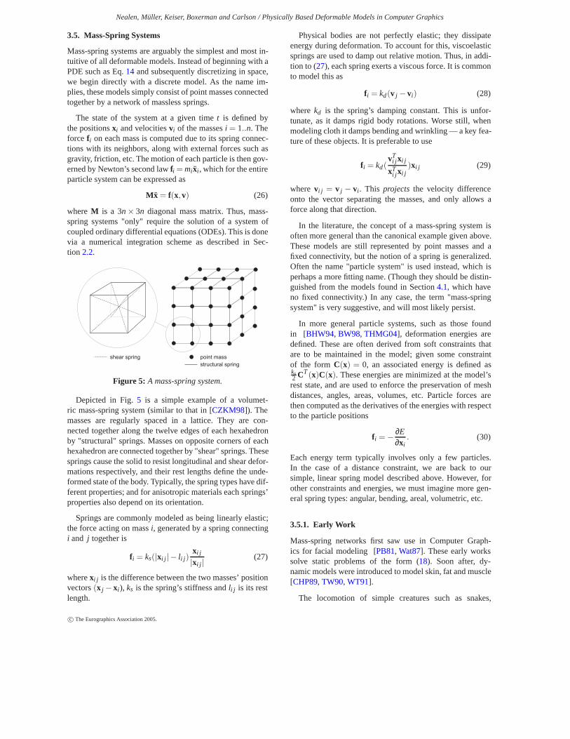
Depicted in Fig.5 is a simple example of a volumet-ric mass-spring system (similar to that in [CZKM98]). Themasses are regularly spaced in a lattice. They are con-nected together along the twelve edges of each hexahedronby "structural" springs. Masses on opposite corners of eachhexahedron are connected together by "shear" springs. Thesesprings cause the solid to resist longitudinal and shear defor-mations respectively, and their rest lengths define the unde-formed state of the body. Typically, the spring types have dif-ferent properties; and for anisotropic materials each springs’properties also depend on its orientation.
Springs are commonly modeled as being linearly elastic;the force acting on massi, generated by a spring connectingi and j together is
fi = ks(|xi j |− li j )xi j
|xi j | (27)
wherexi j is the difference between the two masses’ positionvectors(x j − xi ), ks is the spring’s stiffness andli j is its restlength.
Physical bodies are not perfectly elastic; they dissipateenergy during deformation. To account for this, viscoelasticsprings are used to damp out relative motion. Thus, in addi-tion to (27), each spring exerts a viscous force. It is commonto model this as
fi = kd(v j − vi) (28)
wherekd is the spring’s damping constant. This is unfor-tunate, as it damps rigid body rotations. Worse still, whenmodeling cloth it damps bending and wrinkling — a key fea-ture of these objects. It is preferable to use
fi = kd(vT
i j xi j
xTi j xi j
)xi j (29)
where vi j = v j − vi . This projects the velocity differenceonto the vector separating the masses, and only allows aforce along that direction.
In the literature, the concept of a mass-spring system isoften more general than the canonical example given above.These models are still represented by point masses and afixed connectivity, but the notion of a spring is generalized.Often the name "particle system" is used instead, which isperhaps a more fitting name. (Though they should be distin-guished from the models found in Section4.1, which haveno fixed connectivity.) In any case, the term "mass-springsystem" is very suggestive, and will most likely persist.
In more general particle systems, such as those foundin [BHW94, BW98, THMG04], deformation energies aredefined. These are often derived from soft constraints thatare to be maintained in the model; given some constraintof the form C(x) = 0, an associated energy is defined asks2 CT(x)C(x). These energies are minimized at the model’srest state, and are used to enforce the preservation of meshdistances, angles, areas, volumes, etc. Particle forces arethen computed as the derivatives of the energies with respectto the particle positions
fi = − ∂E∂xi
. (30)
Each energy term typically involves only a few particles.In the case of a distance constraint, we are back to oursimple, linear spring model described above. However, forother constraints and energies, we must imagine more gen-eral spring types: angular, bending, areal, volumetric, etc.
3.5.1. Early Work
Mass-spring networks first saw use in Computer Graph-ics for facial modeling [PB81, Wat87]. These early workssolve static problems of the form (18). Soon after, dy-namic models were introduced to model skin, fat and muscle[CHP89, TW90, WT91].
The locomotion of simple creatures such as snakes,
c© The Eurographics Association 2005.
Nealen, Müller, Keiser, Boxerman and Carlson / Physically Based Deformable Models in Computer Graphics
worms and fish [Mil88, TT94] was simulated using mass-spring systems. In these systems, spring rest-lengths varyover time to simulate muscle actuation.
In work by Terzopoulos et al. [TPF89] the equations ofthermal conductivity are used to simulate heat transfer in avolumetric mass-spring system. Each spring’s stiffness is de-termined by its temperature, which is set to zero once themelting threshold is exceeded. A discrete fluid model (sim-ilar to those presented in Section4.1) is applied to particlesfor which all connecting springs have melted.
Breen et al. [BHW94] presented a particle system tomodel cloth. They posited that cloth is a mechanism of warpand weft fibres — not a continuum — and that mass-springsystems are thusmoreappropriate than Finite Element tech-niques for modeling cloth. Using measured data from theKawabata Evaluation System[Kaw80], they took care in for-mulating their energy functions for stretching, bending andtrellising (shearing), and predicted the static drape of realmaterials quite accurately. Since [BHW94], particle sys-tems have dominated the cloth simulation literature — al-though new FEM formulations (such as the one describedin [EKS03]) continue to be proposed.
3.5.2. Drawbacks and Improvements
Particle systems tend to be intuitive and simple to imple-ment. Moreover, they are computationally efficient and han-dle large deformations with ease. However, unlike the FiniteElement and finite difference methods, which are built uponelasticity theory, mass-spring systems are not necessarily ac-curate. Primarily, most such systems are not convergent; thatis, as the mesh is refined, the simulation does not convergeon the true solution. Instead, the behavior of the model isdependent on the mesh resolution and topology. In practice,spring constantsks are often chosen arbitrarily, and one cansay little quantitatively about the material being modeled. Inaddition, there is often coupling between the various springtypes. For instance, the "shear" springs of the model in Fig.5also resist stretching. For medical applications, as well as forvirtual garment simulation in the textile industry, greater ac-curacy is required. For applications such as film and games,this lack of accuracy may be acceptable; convincing anima-tions have been produced using these systems. However, ajudicious choice of model is still advised, as the behavior ofthe material being modeled can be highly mesh dependent.
Several researchers have explored and have tried tomitigate the accuracy issues in mass-spring systems.Kass [Kas95] presents a simple equivalence in one di-mension between a mass-spring system and a correspond-ing finite difference spatial discretization. Eischen andBigliani [HB00] perform a comparison between a Finite El-ement model and a carefully tuned particle system, whichgave similar experimental results for small deformations. Et-zmuss et al. [EGS03] carefully derive a cloth particle sys-tem from a continuous formulation by a finite difference dis-
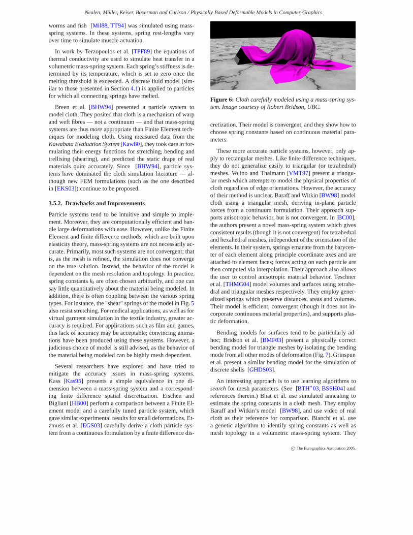
Figure 6: Cloth carefully modeled using a mass-spring sys-tem. Image courtesy of Robert Bridson, UBC.
cretization. Their model is convergent, and they show how tochoose spring constants based on continuous material para-meters.
These more accurate particle systems, however, only ap-ply to rectangular meshes. Like finite difference techniques,they do not generalize easily to triangular (or tetrahedral)meshes. Volino and Thalmann [VMT97] present a triangu-lar mesh which attempts to model the physical properties ofcloth regardless of edge orientations. However, the accuracyof their method is unclear. Baraff and Witkin [BW98] modelcloth using a triangular mesh, deriving in-plane particleforces from a continuum formulation. Their approach sup-ports anisotropic behavior, but is not convergent. In [BC00],the authors present a novel mass-spring system which givesconsistent results (though it is not convergent) for tetrahedraland hexahedral meshes, independent of the orientation of theelements. In their system, springs emanate from the barycen-ter of each element along principle coordinate axes and areattached to element faces; forces acting on each particle arethen computed via interpolation. Their approach also allowsthe user to control anisotropic material behavior. Teschneret al. [THMG04] model volumes and surfaces using tetrahe-dral and triangular meshes respectively. They employ gener-alized springs which preserve distances, areas and volumes.Their model is efficient, convergent (though it does not in-corporate continuous material properties), and supports plas-tic deformation.
Bending models for surfaces tend to be particularly ad-hoc; Bridson et al. [BMF03] present a physically correctbending model for triangle meshes by isolating the bendingmode from all other modes of deformation (Fig.7). Grinspunet al. present a similar bending model for the simulation ofdiscrete shells [GHDS03].
An interesting approach is to use learning algorithms tosearchfor mesh parameters. (See [BTH∗03, BSSH04] andreferences therein.) Bhat et al. use simulated annealing toestimate the spring constants in a cloth mesh. They employBaraff and Witkin’s model [BW98], and use video of realcloth as their reference for comparison. Bianchi et al. usea genetic algorithm to identify spring constants as well asmesh topology in a volumetric mass-spring system. They
c© The Eurographics Association 2005.

Nealen, Müller, Keiser, Boxerman and Carlson / Physically Based Deformable Models in Computer Graphics
Figure 7: A bending model for triangle meshes with nonzerorest angles [BMF03]. The model on the right has signifi-cantly stronger bending resistance, giving it a "water bottle"effect. Image courtesy of Robert Bridson, UBC.
compare their results to FEM reference solutions, and obtainclose correspondence. While such methods are general, theyare computationally expensive and require reference solu-tions; moreover, the results of a specific search may not holdfor different mesh resolutions.
Adaptive meshing techniques are particularly complicatedby the non-convergent behavior of many mass-spring sys-tems, as theyrequiremodeling at multiple resolutions. (An-other difficulty is the handling of so called T-junctions be-tween regions of differing resolutions, though this problemmust also be addressed in FEM and other methods.) A num-ber of authors have addressed this issue for cloth simula-tion. In these systems, splitting/merging criterion are of-ten based on bending angles between triangles. Villard andBorouchaki [VB02] apply adaptive refinement to a simple,convergent model based on quadrilateral meshes. They showconsistent results between meshes of multiple resolutions,maintaining rich detail at reduced computation times. Ear-lier work by Hutchinson et al. [HPH96] takes a similar ap-proach, though the convergence of their model is not clear asthey couple their spatial and time discretizations together inan ad-hoc manner. Li and Volkov [LV05] present an adaptiveframework for triangular cloth meshes, avoiding the prob-lematic T-junctions. They present attractive results, thoughtheir physical model is not convergent.
Finally, a number of researchers have sought to improvethe realism of particle systems by modeling nonlinear mate-rial properties. For instance, Eberhardt et al. [EWS96] basetheir spring model on measured cloth data to model hystere-sis effects; Choi and Ko [CK02] approximate cloth’s buck-ling response using a fifth order polynomial.
3.5.3. Time Integration
Once a force model is chosen, the particle system is steppedforward in time via a numerical integration scheme as in Sec-tion 2.2. Time integration schemes have received particularattention in the cloth simulation literature (see [HES02]).As cloth is often modeled by mass-spring systems, we fur-ther discuss the subject of time integration here.
Cloth is ahighly anisotropic material due to its structure:it resists bending weakly, but has a relatively strong resis-tance to stretching. When simulating a highly stiff volume
of material, one can employ a reduced deformation model,such as modal analysis (see Section5) — and in the limit,use a rigid body model. Clearly, this cannot be done withcloth. We are interested in visualizing the large scale, out-of-plane folding and wrinkling of cloth, however we muststill deal with these planar energies in our model. Numeri-cally speaking, the resulting ODE system (26) is stiff ; thatis, it possesses a wide range of eigenvalues. This forces usto take excessively small time steps when using an explicitscheme.
Provot [Pro95] tackles the issue of stiffness by usingmuch weaker stretching energies and then post-processingthe cloth mesh at each time step, iteratively enforcing con-straints. Springs that are stretched by more than 10% are re-laxed (shortened). This in turn stretches nearby neighboringsprings which are then relaxed, and so on until convergenceis obtained. This, in effect, also models the biphasic natureof cloth — small deformations are resisted weakly until athreshold is reached, whereupon stiffness dramatically in-creases. In practice, this method gives efficient, attractive re-sults, though convergence is not guaranteed.
Baraff and Witkin [BW98] present a linear implicitscheme which allows for large time steps while maintain-ing stability. This has proven to be a robust and efficient so-lution to the stiffness problem, and has become a populartechnique. Specifically, they apply a backward Euler schemeto Eq.26, giving[
∆x∆v
]= ∆t
[vn +∆v
M−1f(xn +∆x,vn +∆v)
](31)
wherexn = x(t) andvn = v(t). This is a nonlinear equationin ∆x and∆v. A linear implicit version of (31) is obtained byusing a first order Taylor series expansion off
f(xn +∆x,vn +∆v) = fn +∂f∂x
∆x +∂f∂v
∆v (32)
where ∂f∂x and ∂f
∂v are the Jacobian matrices of the particleforces with respect to position and velocity respectively. Intheir paper, Baraff and Witkin derive expressions for the Ja-cobians of the various internal forces in their model. Due tothe local connectivity structure of the mesh, these are sparsematrices. They then solve the resulting linear system at eachtime step
A∆v = b, (33)
where
A ≡ (I −∆tM−1 ∂f∂v
−∆t2M−1 ∂f∂x
) (34)
and b ≡ ∆tM−1(fn +∆t∂f∂x
vn). (35)
They solve this system, in the presence of constraints, us-ing a modified preconditioned conjugate gradient solver(MPCG). This is equivalent to applying one Newton itera-tion to Eq.31. Although solving this system increases the
c© The Eurographics Association 2005.

Nealen, Müller, Keiser, Boxerman and Carlson / Physically Based Deformable Models in Computer Graphics
Figure 8: Decomposing cloth into parts which can be solvedmore efficiently [BA04].
computational cost at each time step, this is more than off-set by the ability to take large steps when desired. However,as illustrated by Desbrun et al. [DSB99], the larger the timestep size, the more artificial damping is added to the system.
Others have since attempted to improve upon Baraff andWitkin’s approach. Desbrun et al. [DSB99] precompute thelinear part ofA, achieving anO(n), unconditionally stablescheme. Their technique, however, is inaccurate and doesnot generalize well to large systems. Kang et al. [KCC∗00]improve upon this approximation, but ultimately are only re-placing the CG iterations of [BW98] with a single, Jacobi-like iteration. Volino and Magnenat-Thalmann [VMT00] usea weighted implicit-midpoint method that appeared to giveattractive results, but which is less stable and may be diffi-cult to tune in practice. Choi and Ko [CK02] use the moreaccurate second-order backward difference formula (BDF2);moreover, their coupled compression/bending model im-proves the stability of the system, eliminating the need forfictitious spring damping.
Instead of applying an implicit scheme to the entiresystem, a number of researchers have employed implicit-explicit (IMEX) schemes [ARW95]. The essential idea is toseparately treat the stiff and non-stiff parts of the ODE, han-dling the stiff parts with an implicit method and the non-stiffparts with an explicit method. This combines the stabilityof an implicit scheme where needed with the simplicity andefficiency of an explicit scheme where possible. Hauth etal. [HES02] base their IMEX splitting on connection type:stretch springs are handled implicitly, whereas shear andbend "springs" are handled explicitly. This simplifies imple-mentation and improves the sparsity ofA — and thus thecost of solving Eq.33. The authors also use BDF2, and em-bed their linear solver within a Newton solver, making theirsa fully (as opposed to linear) implicit technique. Boxermanand Ascher [BA04] take a similar approach, optimizing theirIMEX splitting adaptively based on a local stability crite-rion. Each spring is handled either explicitly or implicitly,based on time step, local mesh resolution and material prop-erties. They then take further advantage of the improved sys-tem sparsity to decompose the mesh into components whichcan be solved more efficiently (Fig.8).
Bridson et al. [BMF03] apply a similar IMEX split-ting to cloth as that used for advection-diffusion equa-
tions [ARW95], applying an implicit method to the damp-ing term and an explicit method to the elastic term. This isappropriate when damping plays a significant role, as damp-ing imposes quadratic time step restrictions with respect tomesh size (as opposed to a linear one for elastic terms).They incorporate this within a second order accurate inte-gration scheme, and include a strain limiting step. Coupledwith their careful handling of bending and collisions, theyproduced visually stunning cloth animations.
4. Lagrangian Mesh Free Methods
4.1. Loosely Coupled Particle Systems
Particle systems were developed by Reeves [Ree83] for ex-plosion and subsequent expanding fire simulation in themovie "Star Trek II: The Wrath of Khan". The same tech-nique can also be used for modeling other fuzzy objectssuch as clouds and water, i.e. objects that do not have awell-defined surface. Particles are usually graphical prim-itives such as points or spheres, however, they might alsorepresent complex group dynamics such as a herd of ani-mals [Rey87]. Each particle stores a set of attributes, e.g. po-sition, velocity, temperature, shape, age and lifetime. Theseattributes define the dynamical behavior of the particles overtime and are subject to change due to procedural stochasticprocesses. Particles pass through three different phases dur-ing their lifetime: generation, dynamics and death.
In [Ree83], particles are points in 3D space which rep-resent the volume of an object. A stochastic process gen-erates particles in a predeterminedgeneration shapewhichdefines a region about its origin into which the new parti-cles are randomly placed. Attribute values are either fixed ormay be determined stochastically. Initially, particles moveoutward away from the origin with a random speed. Dur-ing the dynamics phase, particle attributes might change asfunctions of both time and attributes of other particles. Po-sition is updated by simply adding the velocity. Finally, aparticle dies if its lifetime reaches zero or if it does not con-tribute to the animation anymore, e.g. if it is outside of aregion of interest. A particle is rendered as a point lightsource which adds an amount of light depending on its colorand transparency attribute. Motion blurring is very easy toachieve by rendering a particle as a streak using its posi-tion and velocity. An advantage of particles is their simplic-ity, which enables the animation of a huge number of par-ticles for complex scenes. The procedural definition of themodel and its stochastic control simplifies the human de-sign of the system. Furthermore, with particle hierarchies,complicated fuzzy objects such as clouds can be assem-bled and controlled. Although the particles are simulatedomitting inter-particle forces, the resulting animations areconvincing and fast for inelastic phenomena. Therefore, thetechnique has been widely employed in movies and videogames. Examples of modeling waterfalls, ship wakes, break-
c© The Eurographics Association 2005.
Nealen, Müller, Keiser, Boxerman and Carlson / Physically Based Deformable Models in Computer Graphics
ing waves andsplashes using particle systems can be foundin [FR86, Pea86, Gos90, Sim90, OH95].
Particles which interact with each other depending ontheir spatial relationship are referred to as spatially coupledparticle systems [Ton92]. The interactions between parti-cles evolve dynamically over time, thus, complex geome-try and topological changes can be easily modeled usingthis approach. Tonnesen presented a framework for physi-cally based animation of solids and liquids based on dynam-ically coupled particles which represent the volume of anobject [Ton91, Ton98]. Each particlepi has a potential en-ergy φi which is the sum of the pairwise potential energiesφi j betweenpi and all other other particlespj , i.e.
φi = ∑j �=i
φi j . (36)
The forcefi exerted onpi with positionxi is then
fi = −∇xi φi = −∑j �=i
∇xi φi j . (37)
So far, all particles interact with each other, resulting inO(n2) complexity wheren is the number of particles. Thecomputational costs for computing the force can be reducedto O(n) when restricting the interaction to a neighborhoodwithin a certain distance, andO(nlogn) for neighbor search-ing. To avoid discontinuities at the neighborhood bound-ary, the potentials are weighted with a continuous, smoothand monotonically decreasing weighting function which de-pends on the distance to the particles and ranges from one atthe particle position to zero at the neighborhood boundary.
For deriving inter-particle forces, the Lennard-Jones po-tentialφLJ is used:
φLJ(d) =Bdn − A
dm , (38)
whered is the distance between two particles, andn, m, Band A are constants. The Lennard-Jones potential is wellknown in molecular dynamics for modeling the interactionpotential between pairs of atoms. It creates long-range at-tractive and short-range repulsive forces, yielding particlesarranged into hexagonally ordered 2D layers in absence ofexternal forces. A more convenient formulation, called theLennard-Jones bi-reciprocal function, is written as
φ(d) =−eo
m−n(m(
d0
d)n−n(
d0
d)m), (39)
whered0 is theequilibrium separation distance, and−e0 isthe minimal potential (the magnitude is called thedissoci-ation energy). Increasing the dissociation energy increasesthe stiffness of the model, while with the exponentsn andm the width of the potential well can be varied. Therefore,large dissociation energy and high exponents yield rigid andbrittle material, while low dissociation energy and small ex-ponents result in soft and elastic behavior of the object. Thisallows the modeling of a wide variety of physical properties
ranging from stiff to fluid-like behavior. By coupling the dis-sociation energy with thermal energy such that the total sys-tem energy is conserved, objects can be melted and frozen.Furthermore, thermal expansion and contraction can be sim-ulated by adapting the equilibrium separation distanced0 tothe temperature.
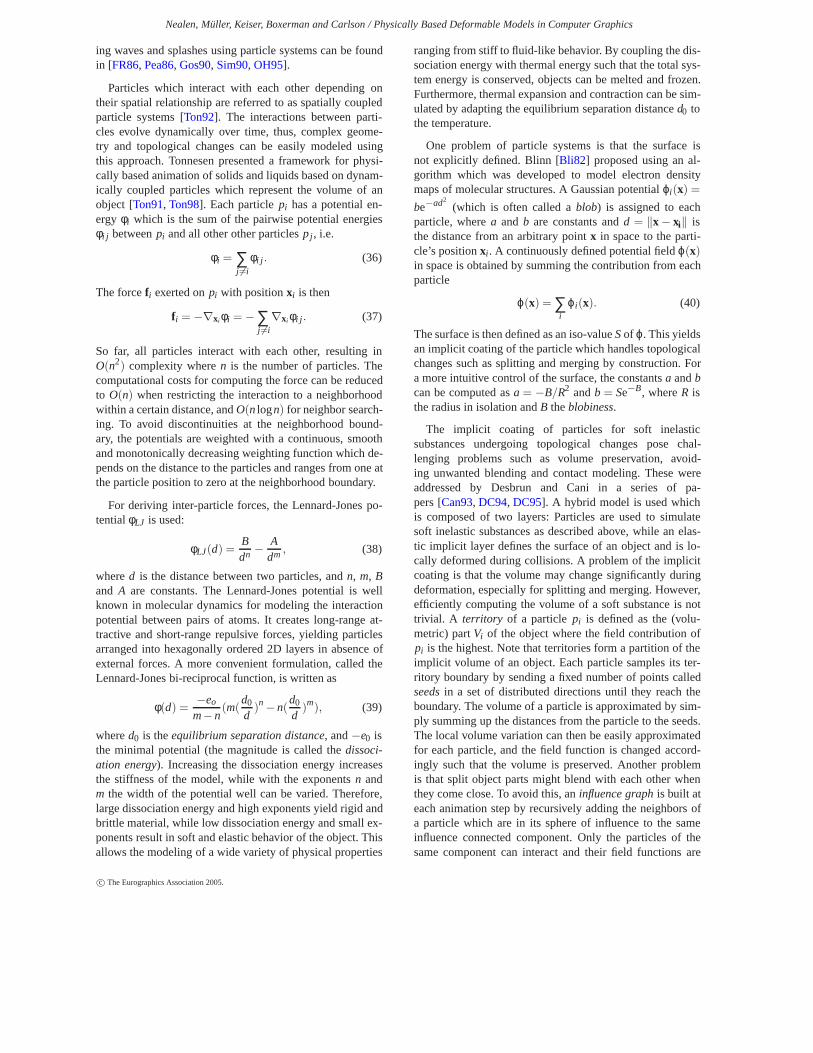
One problem of particle systems is that the surface isnot explicitly defined. Blinn [Bli82] proposed using an al-gorithm which was developed to model electron densitymaps of molecular structures. A Gaussian potentialϕi(x) =be−ad2
(which is often called ablob) is assigned to eachparticle, wherea and b are constants andd = ‖x − xi‖ isthe distance from an arbitrary pointx in space to the parti-cle’s positionxi . A continuously defined potential fieldϕ(x)in space is obtained by summing the contribution from eachparticle
ϕ(x) = ∑i
ϕi(x). (40)
The surface is then defined as an iso-valueSof ϕ. This yieldsan implicit coating of the particle which handles topologicalchanges such as splitting and merging by construction. Fora more intuitive control of the surface, the constantsa andbcan be computed asa = −B/R2 andb = Se−B, whereR isthe radius in isolation andB theblobiness.
The implicit coating of particles for soft inelasticsubstances undergoing topological changes pose chal-lenging problems such as volume preservation, avoid-ing unwanted blending and contact modeling. These wereaddressed by Desbrun and Cani in a series of pa-pers [Can93, DC94, DC95]. A hybrid model is used whichis composed of two layers: Particles are used to simulatesoft inelastic substances as described above, while an elas-tic implicit layer defines the surface of an object and is lo-cally deformed during collisions. A problem of the implicitcoating is that the volume may change significantly duringdeformation, especially for splitting and merging. However,efficiently computing the volume of a soft substance is nottrivial. A territory of a particlepi is defined as the (volu-metric) partVi of the object where the field contribution ofpi is the highest. Note that territories form a partition of theimplicit volume of an object. Each particle samples its ter-ritory boundary by sending a fixed number of points calledseedsin a set of distributed directions until they reach theboundary. The volume of a particle is approximated by sim-ply summing up the distances from the particle to the seeds.The local volume variation can then be easily approximatedfor each particle, and the field function is changed accord-ingly such that the volume is preserved. Another problemis that split object parts might blend with each other whenthey come close. To avoid this, aninfluence graphis built ateach animation step by recursively adding the neighbors ofa particle which are in its sphere of influence to the sameinfluence connected component. Only the particles of thesame component can interact and their field functions are
c© The Eurographics Association 2005.
Nealen, Müller, Keiser, Boxerman and Carlson / Physically Based Deformable Models in Computer Graphics
blended. However, the problem arises that two or more sep-arated components might collide. For detecting a collision,the seed points on the iso-surfaceS are tested against thefield function of another component. For resolving interpen-etrations between two components with potential functionsϕ1 and ϕ2, exact contact surfaces are computed by apply-ing negative compressing potentialsg2,1 andg1,2 such thatϕ1 + g2,1 = ϕ2 + g1,2 = S, resulting in a local compres-sion. To compensate the compression and ensureC1 con-tinuity of the deformed surfaces, positive dilating poten-tials are applied in areas defined around the interpenetrationzone [Can93, OC97]. For collision response, the compres-sion potentialsgi, j are computed for each colliding seed andthen transmitted as response force to the corresponding par-ticle. Additionally, the two components might be merged lo-cally where the collision force exceeds a threshold.
Szeliski and Tonnesen introduced oriented particles fordeformable surface modeling [ST92, Ton98], where eachparticle represents a small surface element (called surfel).Each surfel has a local coordinate frame, given by the po-sition of the particle, a normal vector and a local tangentplane to the surface. To arrange the particles into surface-like arrangements, interaction potentials are defined whichfavor locally planar or locally spherical arrangements. TheLennard-Jones potential described above is used to controlthe average inter-particle spacing. The weighted sum of allpotentials yields the energy of a particle, where the weightscontrol the bending and stiffness of the surface. Variationof the particle energy with respect to its position and ori-entation yields forces acting on the positions and torquesacting on the orientations, respectively. Using these forcesand torques, the Newtonian equations for linear and angularmotion are solved using explicit integration as described inSection2.2.
Recently, Bell et al. presented a method for simulatinggranular materials, such as sand and grains, using a parti-cle system [BYM05]. A (non-spherical) grain is composedof several round particles, which move together as a singlerigid body. Therefore, stick-slip behavior naturally occurs.Molecular dynamics (MD) is used to compute contact forcesfor overlapping particles. The same contact model is used forcollision of granular materials with rigid bodies, or even be-tween rigid-bodies, by simply sampling the rigid body sur-face with particles.
4.2. Smoothed Particle Hydrodynamics
Smoothed Particle Hydrodynamics (SPH) is a Lagrangiantechnique where discrete, smoothed particles are used tocompute approximate values of needed physical quantitiesand their spatial derivatives. Forces can be easily derived di-rectly from the state equations. Furthermore, as a particle-based Lagrangian approach it has the advantage that massis trivially conserved and convection is dispensable. This re-duces both the programming and computational complexity
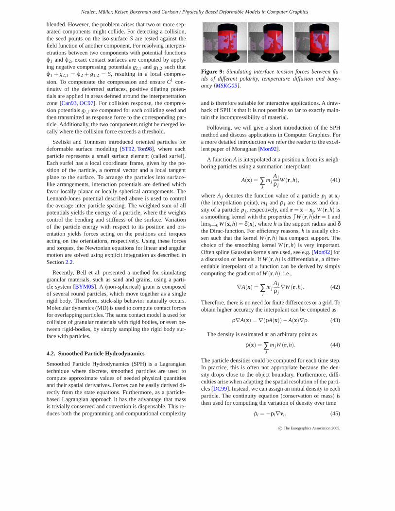
Figure 9: Simulating interface tension forces between flu-ids of different polarity, temperature diffusion and buoy-ancy [MSKG05].
and is therefore suitable for interactive applications. A draw-back of SPH is that it is not possible so far to exactly main-tain the incompressibility of material.
Following, we will give a short introduction of the SPHmethod and discuss applications in Computer Graphics. Fora more detailed introduction we refer the reader to the excel-lent paper of Monaghan [Mon92].
A function A is interpolated at a positionx from its neigh-boring particles using a summation interpolant:
A(x) = ∑j
mjAj
ρ jW(r,h), (41)
whereAj denotes the function value of a particlepj at x j(the interpolation point),mj andρ j are the mass and den-sity of a particlepj , respectively, andr = x− xj. W(r,h) isa smoothing kernel with the properties
�W(r,h)dr = 1 and
limh→0W(x,h) = δ(x), whereh is the support radius andδthe Dirac-function. For efficiency reasons,h is usually cho-sen such that the kernelW(r,h) has compact support. Thechoice of the smoothing kernelW(r,h) is very important.Often spline Gaussian kernels are used, see e.g. [Mon92] fora discussion of kernels. IfW(r,h) is differentiable, a differ-entiable interpolant of a function can be derived by simplycomputing the gradient ofW(r,h), i.e.,
∇A(x) = ∑j
mjAj
ρ j∇W(r,h). (42)
Therefore, there is no need for finite differences or a grid. Toobtain higher accuracy the interpolant can be computed as
ρ∇A(x) = ∇(ρA(x))−A(x)∇ρ. (43)
The density is estimated at an arbitrary point as
ρ(x) = ∑j
mjW(r,h). (44)
The particle densities could be computed for each time step.In practice, this is often not appropriate because the den-sity drops close to the object boundary. Furthermore, diffi-culties arise when adapting the spatial resolution of the parti-cles [DC99]. Instead, we can assign an initial density to eachparticle. The continuity equation (conservation of mass) isthen used for computing the variation of density over time
ρi = −ρi∇vi , (45)
c© The Eurographics Association 2005.
Nealen, Müller, Keiser, Boxerman and Carlson / Physically Based Deformable Models in Computer Graphics
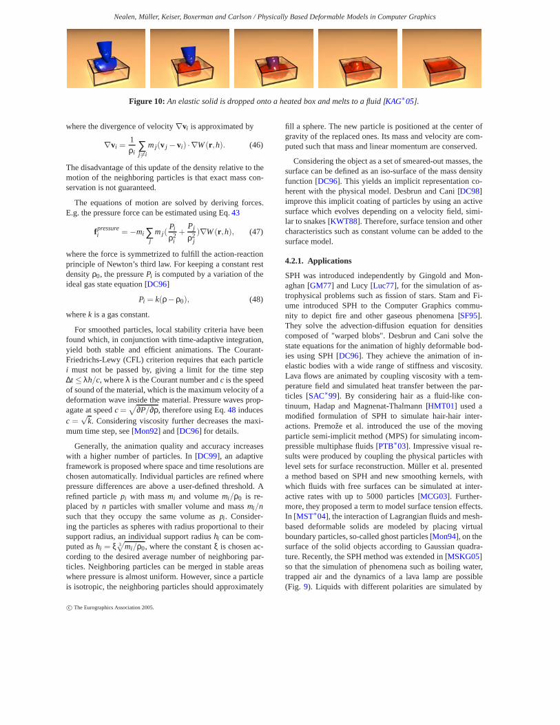
Figure 10: An elastic solid is dropped onto a heated box and melts to a fluid [KAG∗05].
where the divergence of velocity∇vi is approximated by
∇vi =1ρi
∑j �=i
mj(v j − vi) ·∇W(r,h). (46)
The disadvantage of this update of the density relative to themotion of the neighboring particles is that exact mass con-servation is not guaranteed.
The equations of motion are solved by deriving forces.E.g. the pressure force can be estimated using Eq.43
fpressurei = −mi ∑
jmj (
Pi
ρ2i
+Pj
ρ2j
)∇W(r,h), (47)
where the force is symmetrized to fulfill the action-reactionprinciple of Newton’s third law. For keeping a constant restdensityρ0, the pressurePi is computed by a variation of theideal gas state equation [DC96]
Pi = k(ρ−ρ0), (48)
wherek is a gas constant.
For smoothed particles, local stability criteria have beenfound which, in conjunction with time-adaptive integration,yield both stable and efficient animations. The Courant-Friedrichs-Lewy (CFL) criterion requires that each particlei must not be passed by, giving a limit for the time step∆t ≤ λh/c, whereλ is the Courant number andc is the speedof sound of the material, which is the maximum velocity of adeformationwaveinside the material. Pressurewavesprop-agate at speedc =
√∂P/∂ρ, therefore using Eq.48 induces
c =√
k. Considering viscosity further decreases the maxi-mum time step, see [Mon92] and [DC96] for details.
Generally, the animation quality and accuracy increaseswith a higher number of particles. In [DC99], an adaptiveframework is proposed where space and time resolutions arechosen automatically. Individual particles are refined wherepressure differences are above a user-defined threshold. Arefined particlepi with massmi and volumemi/ρ0 is re-placed byn particles with smaller volume and massmi/nsuch that they occupy the same volume aspi . Consider-ing the particles as spheres with radius proportional to theirsupport radius, an individual support radiushi can be com-puted ashi = ξ 3
√mi/ρ0, where the constantξ is chosen ac-
cording to the desired average number of neighboring par-ticles. Neighboring particles can be merged in stable areaswhere pressure is almost uniform. However, since a particleis isotropic, the neighboring particles should approximately
fill a sphere. The new particle is positioned at the center ofgravity of the replaced ones. Its mass and velocity are com-puted such that mass and linear momentum are conserved.
Considering the object as a set of smeared-out masses, thesurface can be defined as an iso-surface of the mass densityfunction [DC96]. This yields an implicit representation co-herent with the physical model. Desbrun and Cani [DC98]improve this implicit coating of particles by using an activesurface which evolves depending on a velocity field, simi-lar to snakes [KWT88]. Therefore, surface tension and othercharacteristics such as constant volume can be added to thesurface model.
4.2.1. Applications
SPH was introduced independently by Gingold and Mon-aghan [GM77] and Lucy [Luc77], for the simulation of as-trophysical problems such as fission of stars. Stam and Fi-ume introduced SPH to the Computer Graphics commu-nity to depict fire and other gaseous phenomena [SF95].They solve the advection-diffusion equation for densitiescomposed of "warped blobs". Desbrun and Cani solve thestate equations for the animation of highly deformable bod-ies using SPH [DC96]. They achieve the animation of in-elastic bodies with a wide range of stiffness and viscosity.Lava flows are animated by coupling viscosity with a tem-perature field and simulated heat transfer between the par-ticles [SAC∗99]. By considering hair as a fluid-like con-tinuum, Hadap and Magnenat-Thalmann [HMT01] used amodified formulation of SPH to simulate hair-hair inter-actions. Premože et al. introduced the use of the movingparticle semi-implicit method (MPS) for simulating incom-pressible multiphase fluids [PTB∗03]. Impressive visual re-sults were produced by coupling the physical particles withlevel sets for surface reconstruction. Müller et al. presenteda method based on SPH and new smoothing kernels, withwhich fluids with free surfaces can be simulated at inter-active rates with up to 5000 particles [MCG03]. Further-more, they proposed a term to model surface tension effects.In [MST∗04], the interaction of Lagrangian fluids and mesh-based deformable solids are modeled by placing virtualboundary particles, so-called ghost particles [Mon94], on thesurface of the solid objects according to Gaussian quadra-ture. Recently, the SPH method was extended in [MSKG05]so that the simulation of phenomena such as boiling water,trapped air and the dynamics of a lava lamp are possible(Fig. 9). Liquids with different polarities are simulated by
c© The Eurographics Association 2005.
Nealen, Müller, Keiser, Boxerman and Carlson / Physically Based Deformable Models in Computer Graphics
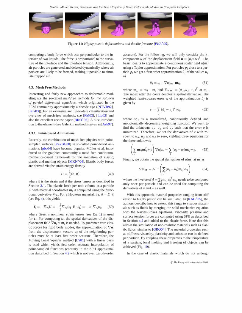
Figure 11: Highly plastic deformations and ductile fracture [PKA∗05].
computing a body force which acts perpendicular to the in-terface of two liquids. The force is proportional to the curva-ture of the interface and the interface tension. Additionally,air particles are generated and deleted dynamically where airpockets are likely to be formed, making it possible to simu-late trapped air.
4.3. Mesh Free Methods
Interesting and fairly new approaches to deformable mod-eling are the so-calledmeshfree methods for the solutionof partial differential equations, which originated in theFEM community approximately a decade ago ([NTVR92],[Suk03]). For an extensive and up-to-date classification andoverview of mesh-free methods, see [FM03], [Liu02] andalso the excellent review paper [BKO∗96]. A nice introduc-tion to the element-free Galerkin method is given in [Ask97].
4.3.1. Point-based Animations
Recently, the combination of mesh-free physics with point-sampled surfaces [PZvBG00] in so-called point-based ani-mations [pba04] have become popular. Müller et al. intro-duced to the graphics community a mesh-free continuum-mechanics-based framework for the animation of elastic,plastic and melting objects [MKN∗04]. Elastic body forcesare derived via the strain energy density
U =12(ε ·σ), (49)
whereε is the strain andσ the stress tensor as described inSection3.1. The elastic force per unit volume at a particlepi with material coordinatesmi is computed using the direc-tional derivative∇ui . For a Hookean material, i.e.σ = E · ε(see Eq.4), this yields
fi = −∇uiU = −12∇ui (εi ·E · εi) = −σ ·∇ui εi, (50)
where Green’s nonlinear strain tensor (see Eq.1) is usedfor εi . For computingεi , the spatial derivatives of the dis-placement field∇ui atmi is needed. To guarantee zero elas-tic forces for rigid body modes, the approximation of∇uifrom the displacement vectorsu j of the neighboring par-ticles must be at least first order accurate. Therefore, theMoving Least Squares method [LS81] with a linear basisis used which yields first order accurate interpolation ofpoint-sampled functions (contrary to the SPH approxima-tion described in Section4.2which is not even zeroth-order
accurate). For the following, we will only consider the x-componentu of the displacement fieldu = (u,v,w)T . Thebasic idea is to approximate a continuous scalar fieldu(m)using a Taylor approximation. For particlespj close to a par-ticle pi we get a first order approximation ˜uj of the valuesujas
uj = ui +∇u|mi ·mi j , (51)
where mi j = m j − mi and ∇u|mi = (u,x,u,y,u,z)T at mi .The index after the coma denotes a spatial derivative. Theweighted least-squares errorei of the approximation ˜uj isgiven by
ei = ∑j
(uj −uj )2wi j , (52)
where wi j is a normalized, continuously defined andmonotonically decreasing weighting function. We want tofind the unknownsu,x, u,y and u,z such that the errore isminimized. Therefore, we set the derivatives ofe with re-spect tou,x, u,y andu,z to zero, yielding three equations forthe three unknowns(
∑j
mi j mTi j wi j
)∇u|mi = ∑
j(uj −ui)mi j wi j . (53)
Finally, we obtain the spatial derivatives ofu(m) atmi as
∇u|mi = A−1
(∑
j(uj −ui)mi j wi j
), (54)
where the inverse ofA=∑ j mi j mTi j wi j needs to be computed
only once per particle and can be used for computing thederivatives ofv andw as well.
With this approach, material properties ranging from stiffelastic to highly plastic can be simulated. In [KAG∗05], theauthors describe how to extend this range to viscous materi-als such as fluids by merging the solid mechanics equationwith the Navier-Stokes equations. Viscosity, pressure andsurface tension forces are computed using SPH as describedin Section4.2 and added to the elastic force. Note that thisallows the simulation of non-realistic materials such as elas-tic fluids, similar to [GBO04]. The material properties suchas stiffness, viscosity, plasticity and cohesion can be definedper particle. By coupling these properties to the temperatureof a particle, local melting and freezing of objects can beachieved (Fig.10).
In the case of elastic materials which do not undergo
c© The Eurographics Association 2005.
Nealen, Müller, Keiser, Boxerman and Carlson / Physically Based Deformable Models in Computer Graphics
any topological changes, the surface can be simply draggedalong with the particles [MKN∗04]. This is done by com-puting the displacement for each surface element (surfel)from the displacements of neighboring particlespj . The firstorder approximation of∇u at m j can be used to obtain asmooth displacement vector field which is invariant underlinear transformations:
x(msi ) = msi +∑j
ω(msi ,m j)(u j +∇u|m j (m j −msi )),
(55)wheremsi andx(msi ) are the material and world coordinatesof a surfelsi , respectively, andω is a normalized weightingkernel. The deformation is computed and applied to both thecenter and the axes of a surfel. To adapt the sampling of thesurface in case of stretching or compression, surfels can besplit or merged similar to [PKKG03]. The animation of thephysics particles combined with this surface skin allows thesimulation of elastic and plastic materials of detailed modelsin real-time. Furthermore, Adams et al. [AKP∗05] showedthat the surface can be efficiently raytraced by exploiting thedeformation field for bounding hierarchy updates.
However, dragging the surface along with the particlesfails if topological changes occur. In this case, an implicitrepresentation can be used as discussed in the Section4.2.In [MKN∗04], this implicit representation is sampled withsurfels. After an animation step the new position of thesurfels is estimated using the displacement computation inEq.55. The deformed surfels are then projected onto the im-plicit surface. Finally, a resampling and relaxation schemeensures that the surface is completely covered and uniformlysampled with surfels. In [KAG∗05], the implicit represen-tation is improved by applying energy potentials and geo-metric constraints which give better control over the surface.However, as the particle representation of the volume is usu-ally much coarser than the surface representation, the im-plicit coating of the particles cannot represent fine detail ofthe surface. A possible solution is to use the explicit defor-mation approach of (55) for solids (with low temperature),the implicit representation for fluids (with high temperature),and blend between the explicit and the implicit representa-tion depending on the temperature for melting object parts.This way, surface detail smoothly fades out and the meltingsurface approaches the implicit representation. Freezing flu-ids are handled analogously.
The framework is extended in [PKA∗05] to cope withfracturing (Fig.11). Cracks are created at surfels where themain principal stress exceeds a threshold. The crack propa-gates in a plane perpendicular to the main principal stress,where the crack surface is dynamically sampled with sur-fels. Visibility tests detect neighboring particles, which areseparated by a crack surface. A splitting, merging and ter-mination operator handles the topological events which oc-cur when cracks merge or branch. Furthermore, a resam-pling scheme adapts the particles resolution to handle smallfractured object pieces. With the suggested methods a wide
range of materials can be fractured, from stiff elastic tohighly plastic objects that exhibit brittle and/or ductile frac-ture.
Collision detection of point-based models has been dis-cussed for rigid [KZ04], quasi-rigid [PPG04] and de-formable objects [KMH∗04]. For rigid collision detection,a bounding sphere hierarchy is built with the surfels asleaves, which is suitable for time-critical collision detec-tion [KZ04]. Pauly et. al [PPG04] compute a consistent con-tact surface and the traction distribution by solving a LinearComplementarity Problem (LCP). Collision response forcesare computed from the local tractions and integration yieldsthe total wrench that acts on the quasi-rigid bodies. Keiser etal. propose to decouple the collision handling and deforma-tion to achieve stable and efficient contact handling for de-formable objects [KMH∗04]. Collisions are detected usinga high resolution surface sampled with surfels and a simplescheme is used to compute a consistent contact surface. Apenalty force depending on its displacement onto the con-tact surface is computed for each surfel. These forces arethen distributed to the neighboring particles where they areapplied as external collision response forces in the next ani-mation step.
Wicke et al. propose a method for animating point-sampled thin shells [WSG05]. The geometric surface prop-erties are approximated using splines (so-calledfibres) em-bedded in the surface. Physical effects such as plasticity andfracturing can be easily modeled. The authors also describea skinning technique for point-sampled surfaces, with whicha high-resolution surface can be animated using a sparse setof samples.
4.3.2. Meshless Deformations Based on Shape Matching
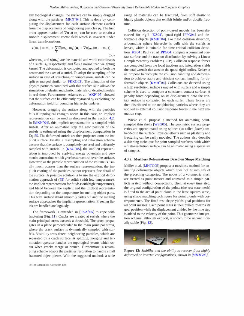
Müller et al. [MHTG05] propose a meshless method for an-imating deformable objects which does not fit into any ofthe preceding categories. The nodes of a volumetric meshare treated as point masses and animated as a simple par-ticle system without connectivity. Then, at every time step,the original configuration of the points (the rest state mesh)is fitted to the actual point cloud in the least squares sense,using shape matching techniques for point clouds with cor-respondence. The fitted rest shape yields goal positions forall point masses. Each point mass is then pulled towards itsgoal position while the displacement divided by the time stepis added to the velocity of the point. This geometric integra-tion scheme, although explicit, is shown to be uncondition-ally stable (Fig.12).
Figure 12: Stability and the ability to recover from highlydeformed or inverted configurations, shown in [MHTG05].
c© The Eurographics Association 2005.
Nealen, Müller, Keiser, Boxerman and Carlson / Physically Based Deformable Models in Computer Graphics
5. Reduced Deformation Models and Modal Analysis
5.1. Basic Formulation
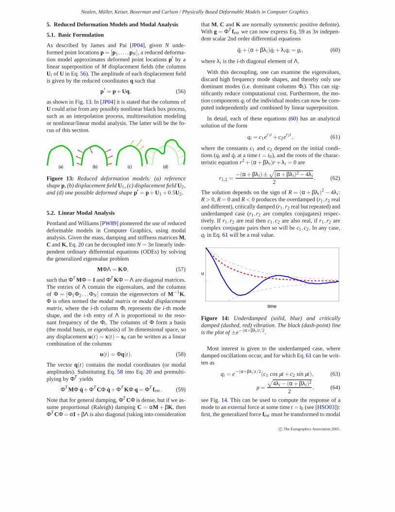
As described by James and Pai [JP04], given N unde-formed point locationsp = [p1, . . . ,pN], a reduced deforma-tion model approximates deformed point locationsp′ by alinear superposition ofM displacement fields (the columnsUi of U in Eq.56). The amplitude of each displacement fieldis given by the reduced coordinatesq such that
p′ = p +Uq, (56)
as shown in Fig.13. In [JP04] it is stated that the columns ofU could arise from any possibly nonlinear black box process,such as an interpolation process, multiresolution modelingor nonlinear/linear modal analysis. The latter will be the fo-cus of this section.
(a) (b) (c) (d)
Figure 13: Reduced deformation models: (a) referenceshapep, (b) displacement fieldU1, (c) displacement fieldU2,and (d) one possible deformed shapep′ = p +U1+0.5U2.
5.2. Linear Modal Analysis
Pentland and Williams [PW89] pioneered the use of reduceddeformable models in Computer Graphics, using modalanalysis. Given the mass, damping and stiffness matricesM,C andK, Eq.20can be decoupled intoN = 3n linearly inde-pendent ordinary differential equations (ODEs) by solvingthe generalized eigenvalue problem
MΦΛ = KΦ, (57)
such thatΦTMΦ= I andΦTKΦ = Λ are diagonal matrices.The entries ofΛ contain the eigenvalues, and the columnsof Φ = [Φ1Φ2 . . .ΦN] contain the eigenvectors ofM−1K.Φ is often termed themodal matrixor modal displacementmatrix, where thei-th columnΦi represents thei-th modeshape, and thei-th entry of Λ is proportional to the reso-nant frequency of theΦi . The columns ofΦ form a basis(the modal basis, oreigenbasis) of 3n dimensional space, soany displacementu(t) = x(t)− x0 can be written as a linearcombination of the columns
u(t) = Φq(t). (58)
The vectorq(t) contains the modal coordinates (or modalamplitudes). Substituting Eq.58 into Eq.20 and premulti-plying by ΦT yields
ΦTMΦ q+ΦTCΦ q+ΦTKΦ q = ΦT fext. (59)
Note that for general damping,ΦTCΦ is dense, but if we as-sume proportional (Raleigh) dampingC = αM + βK, thenΦTCΦ= αI+βΛ is also diagonal (taking into consideration
thatM, C andK are normally symmetric positive definite).With g = ΦT fext we can now express Eq.59 as 3n indepen-dent scalar 2nd order differential equations
qi +(α +βλi)qi +λiqi = gi , (60)
whereλi is thei-th diagonal element ofΛ.
With this decoupling, one can examine the eigenvalues,discard high frequency mode shapes, and thereby only usedominant modes (i.e. dominant columnsΦi ). This can sig-nificantly reduce computational cost. Furthermore, the mo-tion componentsqi of the individual modes can now be com-puted independently and combined by linear superposition.
In detail, each of these equations (60) has an analyticalsolution of the form
qi = c1er1t +c2er2t , (61)
where the constantsc1 andc2 depend on the initial condi-tions (qi andqi at a timet = t0), and the roots of the charac-teristic equationr2 +(α +βλi)r +λi = 0 are
r1,2 =−(α +βλi)±
√(α +βλi)2−4λi
2. (62)
The solution depends on the sign ofR= (α + βλi)2 −4λi :R> 0,R= 0 andR< 0 produces the overdamped (r1, r2 realand different), critically damped (r1, r2 real but repeated) andunderdamped case (r1, r2 are complex conjugates) respec-tively. If r1, r2 are real thenc1,c2 are also real, ifr1, r2 arecomplex conjugate pairs then so will bec1,c2. In any case,qi in Eq.61will be a real value.
time
u
Figure 14: Underdamped (solid, blue) and criticallydamped (dashed, red) vibration. The black (dash-point) lineis the plot of±e−(α+βλi)t/2.
Most interest is given to the underdamped case, wheredamped oscillations occur, and for which Eq.61can be writ-ten as
qi = e−(α+βλi)t/2(c1 cos µt+c2 sin µt), (63)
µ=
√4λi − (α +βλi)2
2, (64)
see Fig.14. This can be used to compute the response of amode to an external force at some timet = t0 (see [HSO03]):first, the generalized forcefext must be transformed to modal
c© The Eurographics Association 2005.
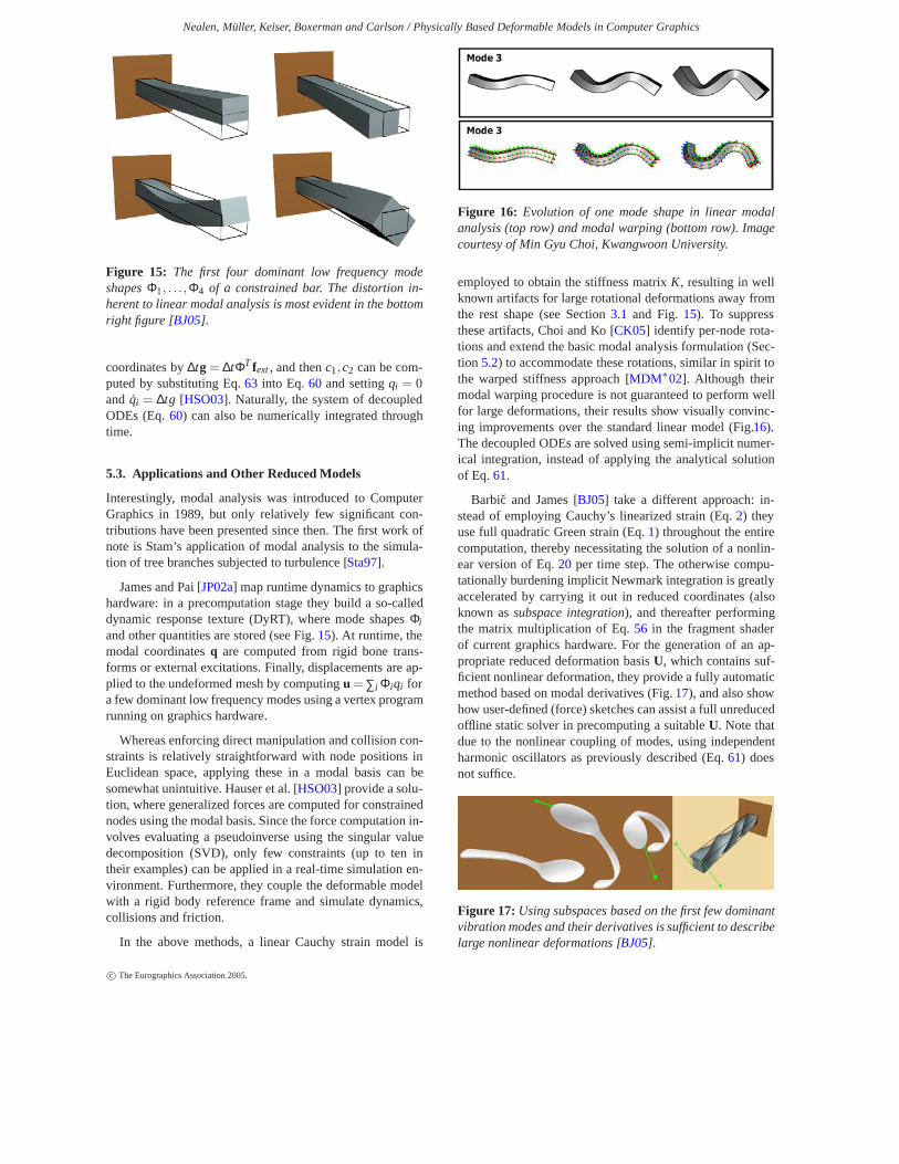
Nealen, Müller, Keiser, Boxerman and Carlson / Physically Based Deformable Models in Computer Graphics
Figure 15: The first four dominant low frequency modeshapesΦ1, . . . ,Φ4 of a constrained bar. The distortion in-herent to linear modal analysis is most evident in the bottomright figure [BJ05].
coordinates by∆tg = ∆tΦT fext, and thenc1,c2 can be com-puted by substituting Eq.63 into Eq.60 and settingqi = 0and qi = ∆tg [HSO03]. Naturally, the system of decoupledODEs (Eq.60) can also be numerically integrated throughtime.
5.3. Applications and Other Reduced Models
Interestingly, modal analysis was introduced to ComputerGraphics in 1989, but only relatively few significant con-tributions have been presented since then. The first work ofnote is Stam’s application of modal analysis to the simula-tion of tree branches subjected to turbulence [Sta97].
James and Pai [JP02a] map runtime dynamics to graphicshardware: in a precomputation stage they build a so-calleddynamic response texture (DyRT), where mode shapesΦi
and other quantities are stored (see Fig.15). At runtime, themodal coordinatesq are computed from rigid bone trans-forms or external excitations. Finally, displacements are ap-plied to the undeformed mesh by computingu =∑i Φiqi fora few dominant low frequency modes using a vertex programrunning on graphics hardware.
Whereas enforcing direct manipulation and collision con-straints is relatively straightforward with node positions inEuclidean space, applying these in a modal basis can besomewhat unintuitive. Hauser et al. [HSO03] provide a solu-tion, where generalized forces are computed for constrainednodes using the modal basis. Since the force computation in-volves evaluating a pseudoinverse using the singular valuedecomposition (SVD), only few constraints (up to ten intheir examples) can be applied in a real-time simulation en-vironment. Furthermore, they couple the deformable modelwith a rigid body reference frame and simulate dynamics,collisions and friction.
In the above methods, a linear Cauchy strain model is
Figure 16: Evolution of one mode shape in linear modalanalysis (top row) and modal warping (bottom row). Imagecourtesy of Min Gyu Choi, Kwangwoon University.
employed to obtain the stiffness matrixK, resulting in wellknown artifacts for large rotational deformations away fromthe rest shape (see Section3.1 and Fig.15). To suppressthese artifacts, Choi and Ko [CK05] identify per-node rota-tions and extend the basic modal analysis formulation (Sec-tion 5.2) to accommodate these rotations, similar in spirit tothe warped stiffness approach [MDM∗02]. Although theirmodal warping procedure is not guaranteed to perform wellfor large deformations, their results show visually convinc-ing improvements over the standard linear model (Fig.16).The decoupled ODEs are solved using semi-implicit numer-ical integration, instead of applying the analytical solutionof Eq.61.
Barbic and James [BJ05] take a different approach: in-stead of employing Cauchy’s linearized strain (Eq.2) theyuse full quadratic Green strain (Eq.1) throughout the entirecomputation, thereby necessitating the solution of a nonlin-ear version of Eq.20 per time step. The otherwise compu-tationally burdening implicit Newmark integration is greatlyaccelerated by carrying it out in reduced coordinates (alsoknown assubspace integration), and thereafter performingthe matrix multiplication of Eq.56 in the fragment shaderof current graphics hardware. For the generation of an ap-propriate reduced deformation basisU, which contains suf-ficient nonlinear deformation, they provide a fully automaticmethod based on modal derivatives (Fig.17), and also showhow user-defined (force) sketches can assist a full unreducedoffline static solver in precomputing a suitableU. Note thatdue to the nonlinear coupling of modes, using independentharmonic oscillators as previously described (Eq.61) doesnot suffice.
Figure 17: Using subspaces based on the first few dominantvibration modes and their derivatives is sufficient to describelarge nonlinear deformations [BJ05].
c© The Eurographics Association 2005.

Nealen, Müller, Keiser, Boxerman and Carlson / Physically Based Deformable Models in Computer Graphics
Figure 18: A silver block catapulting some wooden blocks into an oncoming wall of water [CMT04].
A somewhat different model reduction strategy is devisedby James and Fatahalian [JF03]: they entirely precomputecollision, contact and dynamics (as well as co-parameterizedglobal illumination) of deformable objects by limiting therange of interactions to a finite set of user impulses. The dy-namic responses, termedimpulse response functions(IRFs),each a chronological set of generalized deformation vec-tors, are dimensionality reduced using principal componentanalysis (PCA). At runtime, IRFs are blended based on userinteraction.
6. Eulerian and Semi-Lagrangian Methods
There are two general points of view we can take whendescribing an object that we wish to physically simulate.The main distinctions of the two view points is how theydiscretize an object in order to work with it numerically,and how they define the boundary of the object itself. Sofar, this report has covered theLagrangianpoint of view.As Section2 explains, the Lagrangian point of view de-scribes an object as a set of moving points (material coordi-nates) that travel around and change position over time; thesepoints carry their material properties with them as they movethrough the world. Lagrangian techniques are a convenientway to define an object as a connected mesh of points (Sec-tion 3) or simply a cloud of points (Section4). TheEulerianpoint of view, on the other hand, looks at a stationary setof points and calculates how the material properties storedat those stationary grid points change over time. One of thedrawbacks of changing to an Eulerian perspective is that theboundary of the object is no longer explicitly defined. Thissection covers Eulerian techniques as they are used in Com-puter Graphics, and focuses heavily on fluids because flu-ids are often defined in an Eulerian framework. This sectionwill also explore how object boundaries are represented inthe Eulerian framework. This section is not meant to givean exhaustive reference for Eulerian techniques; it is meantto give the reader an idea of what types of deformable andfuzzy objects have been simulated in an Eulerian framework.
The Eulerian approach to fluids was popularized by a se-ries of papers by Foster and Metaxas [FM96], [FM97b], and[FM97a]. Their formulation solves the fluid (Navier-Stokes)equations on a regular voxel grid and uses a finite differ-
ence formulation for all the differential equations. To un-derstand the Eulerian framework, and how it differs froma Lagrangian one, we will look briefly at how the Navier-Stokes equations (equations of motion for a fluid) are for-mulated and solved for a single time step. We refer thereader to [Car04] for an in-depth discussion of liquids, andto [Sta03] for a practical implementation of a smoke simula-tor.
There are two parts to the Navier-Stokes equations:
∇·u = 0 (65)
ut = −(u ·∇)u +∇· (ν∇u)−∇p+ f. (66)
These two equations represent the conservation of mass andmomentum for an incompressible fluid. The vector fieldut isthe time derivative of the fluid velocity. The scalar pressurefield is p†, andν is the kinematic viscosity. The vector fieldfrepresents the body force per unit mass (usually just gravity).In this Eulerian formulation the quantities of the fluid arestored in a grid of cells (a regular grid of cubes or voxelsif you like). The velocity is stored on the cell faces and thepressure is stored at the center of the cells. This is commonlycalled a staggered (or MAC) grid. Notice that the position,x, of the fluid is not defined; in this Eulerian frame work, thegrid positions remain fixed.
Solving equations65 and 66 is usually done in severalsteps (breaking up a PDE into simpler pieces and solving thepieces separately is known asoperator splitting). Thef termis simply scaled by the time step and added to the currentvelocity. The advection term,−(u ·∇)u, is then solved. Onepopular way to solve the advection term is with thesemi-Lagrangiantechnique [Sta99] because it is stable for largetime step sizes. The semi-Lagrangian technique continues asfollows–to solve for the advection of any quantity through avelocity field (in this case we are solving for the advection ofthe velocity field through itself), the velocity at the grid pointwe wish to update is found, and a path is traced from the gridpoint backwards in time with that velocity to a new location.
† In this formulation we assume a constant density and absorb itinto the pressure term for simplicity.
c© The Eurographics Association 2005.
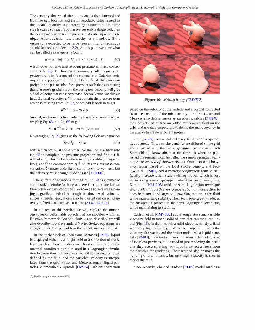
Nealen, Müller, Keiser, Boxerman and Carlson / Physically Based Deformable Models in Computer Graphics
The quantity that we desire to update is then interpolatedfrom the new location and that interpolated value is used asthe updated quantity. It is interesting to note that if the timestep is scaled so that the path traverses only a single cell, thenthe semi-Lagrangian technique is a first order upwind tech-nique. After advection, the viscosity term is solved. If theviscosity is expected to be large then an implicit techniqueshould be used (see Section2.2). At this point we have whatcan be called abest guess velocity:
u = u +∆t[−(u ·∇)u +∇· (ν∇u)+ f], (67)
which does not take into account pressure or mass conser-vation (Eq.65). The final step, commonly called apressure-projection, is in fact one of the reasons that Eulerian tech-niques are popular for fluids. The trick of the pressure-projection step is to solve for a pressure such that subtractingthat pressure’s gradient from the best guess velocity will givea final velocity that conserves mass. So, we know two things:first, the final velocity,unew, must contain the pressure termwhich is missing from Eq.67, so we add it back in to get
unew= u−∆t∇p. (68)
Second, we know the final velocity has to conserve mass, sowe plug Eq.68 into Eq.65 to get
∇·unew= ∇· u−∆t∇· (∇p) = 0. (69)
Rearranging Eq.69 gives us the following Poisson equation
∆t∇2p = ∇· u (70)
with which we must solve forp. We then plugp back intoEq. 68 to complete the pressure projection and find our fi-nal velocity. The final velocity is incompressible (divergencefree), and for a constant density fluid this ensures mass con-servation. Compressible fluids can also conserve mass, buttheir density must change to do so (see [YOH00]).
The system of equations formed by Eq.70 is symmetricand positive definite (as long as there is at least one knownDirichlet boundary condition), and can be solved with a con-jugate gradient method. Although the above explanation as-sumes a regular grid, it can also be carried out on an adap-tively refined grid, such as an octree [SY02, LGF04].
In the rest of this section we will explore the numer-ous types of deformable objects that are modeled within anEulerian framework. As the techniques are described we willalso describe how the standard Navier-Stokes equations arechanged in each case, and how the objects are represented.
In the early work of Foster and Metaxas [FM96] liquidis displayed either as a height field or a collection of mass-less particles. These massless particles are different from thematerial coordinate particles used in a Lagrangian simula-tion because they are passively moved in the velocity fielddefined by the fluid, and the particles’ velocity is interpo-lated from the grid. Foster and Metaxas render liquid par-ticles as smoothed ellipsoids [FM97a] with an orientation
Figure 19: Melting bunny [CMVT02].
based on the velocity of the particle and a normal computedfrom the position of the other nearby particles. Foster andMetaxas also define smoke as massless particles [FM97b]:they advect and diffuse an added temperature field on thegrid, and use that temperature to define thermal buoyancy inthe smoke to create turbulent motion.
Stam [Sta99] uses a scalar density field to define quanti-ties of smoke. These smoke densities are diffused on the gridand advected with the semi-Lagrangian technique (whichStam did not know about at the time, so when he pub-lished his seminal work he called the semi-Lagrangian tech-nique themethod of characteristics). Stam also adds buoy-ancy forces based on the local smoke density, and Fed-kiw et al. [FSJ01] add avorticity confinementterm to arti-ficially increase small scale swirling motion which is lostwhen using semi-Lagrangian advection on coarse grids.Kim et al. [KLLR05] used the semi-Lagrangian techniquewith back and fourth error compensation and correctiontokeep both small and large scale swirling motion in the fluidwhile maintaining stability. Their technique greatly reducesthe dissipation present in the semi-Lagrangian technique,while maintaining its stability.
Carlson et al. [CMVT02] add a temperature and variableviscosity field to model solid objects that can melt into liq-uid (Fig.19). In their model, a solid object is simply a fluidwith very high viscosity, and as the temperature rises theviscosity decreases, and the object melts into a liquid state.Like [FM96], the object in their simulation is defined by a setof massless particles, but instead of just rendering the parti-cles they use a splatting technique to extract a mesh fromthe particles for rendering. Their method also animates thebuilding of a sand castle, but only high viscosity is used tomodel the mud.
More recently, Zhu and Bridson [ZB05] model sand as a
c© The Eurographics Association 2005.
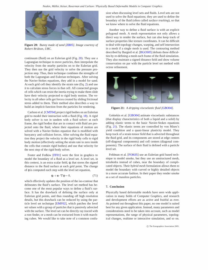
Nealen, Müller, Keiser, Boxerman and Carlson / Physically Based Deformable Models in Computer Graphics
Figure 20: Bunny made of sand [ZB05]. Image courtesy ofRobert Bridson, UBC.
continuum (fluid) on an Eulerian grid (Fig.20). They use aLagrangian technique to move particles, then interpolate thevelocity from the nearby particles on to the Eulerian grid.They then use the grid velocity to solve the pressure pro-jection step. Thus, their technique combines the strengths ofboth the Lagrangian and Eulerian techniques. After solvingthe Navier-Stokes equations, they add in a model for sand.At each grid cell they identify the strain rate (Eq.2) and useit to calculate stress forces in that cell. All connected groupsof cells which can resist the inertia trying to make them slidehave their velocity projected to rigid body motion. The ve-locity in all other cells get forces created by sliding frictionalstress added to them. Their method also describes a way tobuild an implicit function from the particles for rendering.
Carlson et al. [CMT04] project rigid bodies on an Euleriangrid to model their interaction with a fluid (Fig.18). A rigidbody solver is run in tandem with a fluid solver: at eachframe, the rigid bodies that are in contact with fluid are pro-jected onto the fluid, where their equations of motion aresolved with a Navier-Stokes equation that is modified withbuoyancy and collision forces. After solving the fluid equa-tion they project the velocity in the rigid body cells to rigidbody motion (effectively setting the strain rate to zero insidethe cells that contain rigid bodies) and use that velocity forthe next step of the rigid body solver.
Foster and Fedkiw [FF01] were the first in graphics tomodel the boundary of a fluid as a level set. A level set, inthis context, is an extra scalar field,φ, that stores the signeddistance to the fluid surface at each grid point. The changeof φ is computed each step with the level set equation,
φt +u ·∇φ= 0, (71)
which effectively updates the position of the iso-contour thatdelineates the fluid’s surface. The level set method has be-come one of the most popular ways to define a fluid’s sur-face. It has the drawback of defining the surface only atEulerian grid points, and thus rounding off high resolutiondetails, but this drawback can be reduced by using the par-ticle level set technique [EMF02], which patches the levelset values with a group of particles that is passively advectedwith the surface. The level set can be directly ray traced witha root finder, or a mesh can be extracted from it with march-ing cubes. We would like to take note of a common confu-
sion when discussing level sets and fluids. Level sets are notused to solve the fluid equations; they are used to define theboundary of the fluid (often calledsurface tracking), so thatwe know where to solve the fluid equations.
Another way to define a fluid surface is with an explicitpolygonal mesh. A mesh representation not only allows adirect way to render the surface, but can also keep track ofsurface properties like texture coordinates. It can be difficultto deal with topology changes, warping, and self intersectionin a mesh if a single mesh is used. The contouring methoddescribed by Bargteil et al. [BGOS05] defeats these difficul-ties by re-defining a mesh each frame of the fluid simulation.They also maintain a signed distance field and show volumeconservation on par with the particle level set method withoctree refinement.
Figure 21: A dripping viscoelastic fluid [GBO04].
Goktekin et al. [GBO04] animate viscoelastic substances(that display characteristics of both a liquid and a solid) byadding elastic terms to the basic Navier-Stokes equations(Fig. 21). The elastic terms are controlled by von Mises’syield condition and a quasi-linear plasticity model. Theykeep track of a strain tensor field that is advected throughoutthe fluid grid, and its components are stored at edge centers(off-diagonal components) and cell centers (diagonal com-ponents). The surface of their fluid is defined with a particlelevel set.
Feldman et al. [FOK05] use an Eulerian grid based tech-nique to model smoke, but they use an unstructured mesh,tetrahedra instead of cubes, near the boundary of compli-cated objects. Theirhybrid meshformulation allows them tomodel the boundary with curved or highly detailed objectsin a more accurate fashion. In their paper they render smokeas a set of massless particles.
7. Conclusion
Physically based deformable models have seen wide appli-cation in many fields of Computer Graphics, and researchand development efforts are as active and fruitful as ever.As pointed out throughout this paper, no one model is suitedbest for any given application. Instead, many parameters andconsiderations need to be taken into account, such as modelrepresentations, the range of physical parameters, topolog-ical changes, realtime or interactive simulation, and so on.
c© The Eurographics Association 2005.

Nealen, Müller, Keiser, Boxerman and Carlson / Physically Based Deformable Models in Computer Graphics
And even though such a seemingly exhaustive toolkit exists,with which very impressive results have been achieved, westill have quite a way to go until we can plausibly and in-teractively simulate the natural phenomena in our everydaylives. To quote Richard Feynman [FLS63]
"The things with which we concern ourselves inscience appear in myriad forms, and with a mul-titude of attributes. For example, if we stand onthe shore and look at the sea, we see the water,the wavesbreaking, the foam, the sloshing motionof the water, the sound, the air, the winds and theclouds, the sun and the blue sky, and light; thereis sand and there are rocks of various hardnessand permanence, color and texture. There are an-imals and seaweed, hunger and disease, and theobserver on the beach; there may be even happi-ness and thought. Any other spot in nature has asimilar variety of things and influences. It is al-ways as complicated as that, no matter where itis. Curiosity demands that we ask questions, thatwe try to put things together and try to understandthis multitude of aspects as perhaps resulting fromthe action of a relatively small number of elemen-tal things and forces acting in an infinite variety ofcombinations."
We think it is safe to say that this statement still holds, andprobably will hold for years to come, a burden and a blessingalike to researchers in the field.
Yet even with the current methodology, the algorithmsand models have seen somewhat limited application inproduction environments and video games. One reasonfor this is the lack of computational power: many of thepresented techniques are inherently offline, and can takehours or days to produce results. In the field of interactiveentertainment, small physically based deformable modelsare already being implemented, and thanks to developmentssuch as the upcoming physics processing unit (PPU), thistrend is likely to carry on. A second reason we see for areluctancy to adopt these new methods is the limited controlthe users have over the resulting animations. Althoughthis has been previously addressed, we see great potentialin coupling more intuitive user interfaces with physicallybased simulations.
Acknowledgements. We would like to thank the followingpeople for their contributions, suggestions and general helpin shaping and improving this paper: Bart Adams, AdamBargteil, Robert Bridson, Min Gyu Choi, Nico Galoppo andDoug James.
References[AKP∗05] ADAMS B., KEISER R., PAULY M., GUIBAS L. J., GROSSM., DUTRÉ P.:
Efficient raytracing of deforming point-sampled surfaces. InProceedingsof Eurographics(2005). To appear.15
[AP98] ASCHER U., PETZOLD L.: Computer Methods for Ordinary DifferentialEquations and Differential-Algebraic Equations. Society for Industrial &Applied Mathematics, 1998.3
[ARW95] ASCHERU., RUUTH S., WETTON B.: Implicit-explicit methods for time-dependent pde’s.SIAM J. Numer. Anal., 32 (1995), 797–823.10
[Ask97] ASKES H.: Everything you always wanted to know about the Element-FreeGalerkin method, and more. Tech. rep., TU Delft nr. 03.21.1.31.29, 1997.14
[BA04] BOXERMAN E., ASCHER U.: Decomposing cloth. InSCA ’04: Proceed-ings of the 2004 ACM SIGGRAPH/Eurographics symposium on Computeranimation(2004), pp. 153–161.10
[BC00] BOURGUIGNON D., CANI M.-P.: Controlling anisotropy in mass-springsystems. InComputer Animation and Simulation ’00(2000), pp. 113–123.8
[BGOS05] BARGTEIL A. W., GOKTEKIN T. G., O’BRIEN J. F., STRAIN J. A.: Asemi-lagrangian contouring method for fluid simulation.ACM Transactionson Graphics (in press)(2005).20
[BHW94] BREEN D., HOUSE D., WOZNY M.: Predicting the drape of woven clothusing interacting particles. InSIGGRAPH ’94(1994), pp. 365–372.7, 8
[BJ05] BARBIC J., JAMES D. L.: Real-time subspace integration for St.Venant-Kirchhoff deformable models.ACM Transactions on Computer Graphics(ACM SIGGRAPH 2005) 24, 3 (2005).17
[BK04] BOTSCH M., KOBBELT L.: An intuitive framework for real-time freeformmodeling.ACM Trans. Graph. 23, 3 (2004), 630–634.2
[BK05] BOTSCHM., KOBBELT L.: Real-time shape editing using radial basis func-tions. InEurographics 2005, to appear(2005).2
[BKO∗96] BELYTSCHKO T., KRONGAUZ Y., ORGAN D., FLEMING M., KRYSL P.:Meshless methods: An overview and recent developments.Computer Meth-ods in Applied Mechanics and Engineering 139, 3 (1996), 3–47.14
[Bli82] B LINN J. F.: A generalization of algebraic surface drawing.ACM Trans.Graph. 1, 3 (1982), 235–256.11
[BLM00] B ELYTSCHKO T., LIU W. K., MORAN B.: Nonlinear Finite Elements forContinua and Structures. John Wiley & Sons Ltd., 2000.2
[BMF03] BRIDSON R., MARINO S., FEDKIW R.: Simulation of clothing with foldsand wrinkles. InACM SIGGRAPH/Eurographics Symposium ComputerAnimation(2003), pp. 28–36.8, 9, 10
[BNC96] BRO-NIELSEN M., COTIN S.: Real-time volumetric deformable modelsfor surgery simulation using finite elements and condensation.ComputerGraphics Forum 15, 3 (1996), 57–66.5
[BSSH04] BIANCHI G., SOLENTHALER B., SZÉKELY G., HARDERS M.: Simulta-neous topology and stiffness identification for mass-spring models based onfem reference deformations. InMICCAI (2) (2004), pp. 293–301.8
[BTH∗03] BHAT K., TWIGG C., HODGINS J. K., KHOSLA P., POPOVIC Z., SEITZ
S.: Estimating cloth simulation parameters from video. InACM SIG-GRAPH/Eurographics Symposium on Computer Animation(July 2003).8
[BW97] BONET J., WOOD R. D.: Nonlinear continuum mechanics for finite ele-ment analysis. Cambridge Univ. Press, NY, 1997.2
[BW98] BARAFF D., WITKIN A.: Large steps in cloth simulation. InProceedingsof SIGGRAPH 1998(1998), pp. 43–54.7, 8, 9, 10
[BYM05] B ELL N., YOU Y., MUCHA P. J.: Particle-based simulation of granularmaterials. ACM. to appear.12
[Can93] CANI M.-P.: An implicit formulation for precise contact modeling betweenflexible solids. InSIGGRAPH ’93(1993), pp. 313–320.11, 12
[Car04] CARLSON M. T.: Rigid, Melting, and Flowing Fluid. PhD thesis, GeorgiaInstitute of Technology, 2004.18
[CDA99] COTIN S., DELINGETTE H., AYACHE N.: Real-time elastic deformationsof soft tissues for surgery simulation. InIEEE Transactions on Visualizationand Computer Graphics, vol. 5 (1). 1999, pp. 62–73.5
[CDA00] COTIN S., DELINGETTE H., AYACHE N.: A hybrid elastic model allowingreal-time cutting, deformations and force-feedback for surgery training andsimulation.The Visual Computer 16, 8 (2000), 437–452.5
[CEO∗93] COVER S., EZQUERRA N., O’BRIEN J., ROWE R., GADACZ T., PALM
E.: Interactively deformable models for surgery simulation.IEEE Com-puter Graphics and Applications 13, 6 (1993), 68–75.5
[CGC∗02] CAPELL S., GREEN S., CURLESS B., DUCHAMP T., POPOVIC Z.: In-teractive skeleton-driven dynamic deformations. InProceedings of SIG-GRAPH 2002(2002), pp. 586–593.5
c© The Eurographics Association 2005.
Nealen, Müller, Keiser, Boxerman and Carlson / Physically Based Deformable Models in Computer Graphics
[CHP89] CHADWICK J., HAUMANN D., PARENT R.: Layered construction for de-formable animated characters. InSIGGRAPH ’89(1989), pp. 243–252.7
[Chu96] CHUNG T. J.: Applied Continuum Mechanics. Cambridge Univ. Press, NY,1996.2
[CK02] CHOI K.-J., KO H.-S.: Stable but responsive cloth. InSIGGRAPH ’02(2002), pp. 604–611.9, 10
[CK05] CHOI M. G., KO H.-S.: Modal warping: Real-time simulation of large ro-tational deformation and manipulation.IEEE Transactions on Visualizationand Computer Graphics 11, 1 (2005), 91–101.17
[CMT04] CARLSON M., MUCHA P. J., TURK G.: Rigid fluid: Animating the inter-play between rigid bodies and fluid.ACM Transactions on Graphics 23, 3(Aug. 2004), 377–384.18, 20
[CMVT02] CARLSON M., MUCHA P., VAN HORN III R. B., TURK G.: Meltingand flowing. InProceedings of the 2002 ACM SIGGRAPH Symposium onComputer Animation(July 2002), pp. 167–174.19
[Coo95] COOK R. D.: Finite Element Modeling for Stress Analysis. John Wiley &Sons, NY, 1995.2
[CZKM98] CHEN Y., ZHU Q., KAUFMAN A., MURAKI S.: Physically-based ani-mation of volumetric objects. InCA ’98: Proceedings of the ComputerAnimation(1998), p. 154.7
[DC94] DESBRUN M., CANI M.-P.: Highly deformable material for animationand collision processing. InFifth Eurographics Workshop on Animation,Simulation(septembre 1994).11
[DC95] DESBRUN M., CANI M.-P.: Animating soft substances with implicit sur-faces. InComputer Graphics Proceedings(1995), ACM SIGGRAPH,pp. 287–290.11
[DC96] DESBRUN M., CANI M.-P.: Smoothed particles: A new paradigm for ani-mating highly deformable bodies. In6th Eurographics Workshop on Com-puter Animation and Simulation ’96(1996), pp. 61–76.13
[DC98] DESBRUN M., CANI M.-P.: Active implicit surface for animation. InProceedings of Graphics Interface(1998), pp. 143–150.13
[DC99] DESBRUN M., CANI M.-P.: Space-Time Adaptive Simulation of HighlyDeformable Substances. Tech. rep., INRIA Nr. 3829, 1999.12, 13
[DDBC99] DEBUNNE G., DESBRUN M., BARR A., CANI M.-P.: Interactive mul-tiresolution animation of deformable models. InEurographics Workshopon Computer Animation and Simulation ’99(1999), pp. 133–144.5
[DDCB00] DEBUNNE G., DESBRUN M., CANI M.-P., BARR A. H.: Adaptive sim-ulation of soft bodies in real-time. InComputer Animation ’00(2000),pp. 15–20.5
[DDCB01] DEBUNNE G., DESBRUN M., CANI M.-P., BARR A.: Dynamic real-timedeformations using space & time adaptive sampling. InComputer GraphicsProceedings(Aug. 2001), Annual Conference Series, ACM SIGGRAPH2001, pp. 31–36.4, 5
[DSB99] DESBRUNM., SCHRÖDERP., BARR A. H.: Interactive animation of struc-tured deformable objects. InGraphics Interface ’99(1999). 5, 10
[EGS03] ETZMUSS O., GROSSJ., STRASSERW.: Deriving a particle system fromcontinuum mechanics for the animation of deformable objects.IEEE Trans-actions on Visualization and Computer Graphics 9, 4 (2003), 538–550.8
[EKS03] ETZMUSS O., KECKEISEN M., STRASSER W.: A fast finite element so-lution for cloth modelling. Proceedings of Pacific Graphics 2003(2003).8
[EMF02] ENRIGHT D., MARSCHNER S., FEDKIW R.: Animation and rendering ofcomplex water surfaces. InSIGGRAPH ’02(2002), pp. 736–744.20
[EWS96] EBERHARDT B., WEBER A., STRASSER W.: A fast, flexible, particle-system model for cloth draping.IEEE Comput. Graph. Appl. 16, 5 (1996),52–59.9
[FF01] FOSTERN., FEDKIW R.: Practical animation of liquids. InProceedings ofACM SIGGRAPH 2001(2001), pp. 23–30.20
[FLS63] FEYNMAN R. P., LEIGHTON R. B., SANDS M.: The Feynman Lectureson Physics: Volume I. Addison Wesley, 1963.21
[FM96] FOSTERN., METAXAS D.: Realistic animation of liquids.Graphical Mod-els and Image Processing 58, 5 (1996), 471–483.18, 19
[FM97a] FOSTER N., METAXAS D.: Controlling fluid animation. InProceedingsCGI ’97 (1997), pp. 178–188. Winner of the Androme Award 1997.18, 19
[FM97b] FOSTER N., METAXAS D.: Modeling the motion of a hot, turbulent gas.In SIGGRAPH ’97(1997), pp. 181–188.18, 19
[FM03] FRIES T.-P., MATTHIES H. G.: Classification and Overview of MeshfreeMethods. Tech. rep., TU Brunswick, Germany Nr. 2003-03, 2003.14
[FOK05] FELDMAN B. E., O’BRIEN J. F., KLINGNER B. M.: Animating gaseswith hybrid meshes. InProceedings of ACM SIGGRAPH 2005(2005),p. (in press).20
[FR86] FOURNIER A., REEVES W. T.: A simple model of ocean waves. InSIG-GRAPH ’86(1986), pp. 75–84.11
[FSJ01] FEDKIW R., STAM J., JENSEN H. W.: Visual simulation of smoke. InSIGGRAPH ’01(2001), pp. 15–22.19
[GBO04] GOKTEKIN T. G., BARGTEIL A. W., O’BRIEN J. F.: A method for an-imating viscoelastic fluids. InProc. of ACM SIGGRAPH(2004), vol. 23,pp. 463–468.14, 20
[Gdo93] GDOUTOS E. E.: Fracture Mechanics. Kluwer Academic Publishers,Netherlands, 1993.2
[GHDS03] GRINSPUN E., HIRANI A. N., DESBRUN M., SCHRÖDER P.: Discreteshells. InProceedings of the 2003 ACM SIGGRAPH/Eurographics Sympo-sium on Computer animation(2003), pp. 62–67.8
[GKS02] GRINSPUN E., KRYSL P., SCHRÖDER P.: CHARMS: A simple frame-work for adaptive simulation. InProceedings of SIGGRAPH 2002(2002),pp. 281–290.5
[GM77] GINGOLD R. A., MONAGHAN J. J.: Smoothed particle hydrodynamics -theory and application to non-spherical stars.Royal Astronomical Society,Monthly Notices 181(1977), 375–389.13
[GM97] GIBSON S. F., MIRTICH B.: A survey of deformable models in computergraphics. Technical Report TR-97-19, MERL, Cambridge, MA, 1997.1, 2
[Gos90] GOSSM. E.: Motion simulation: A real time particle system for display ofship wakes.IEEE Comput. Graph. Appl. 10, 3 (1990), 30–35.11
[GTT89] GOURRET J.-P., THALMANN N. M., THALMANN D.: Simulation of ob-ject and human skin formations in a grasping task. InSIGGRAPH ’89(1989), pp. 21–30.5
[HB00] HOUSE D., BREEN D.: Cloth modeling and animation. A. K. Peters, Ltd.,2000.2, 8
[HES02] HAUTH M., ETZMUSS O., STRASSERW.: Analysis of numerical methodsfor the simulation of deformable models.The Visual Computer(2002).Accepted for publication.3, 9, 10
[HMT01] HADAP S., MAGNENAT-THALMANN N.: Modeling dynamic hair as con-tinuum. InEurographics Proceedings. Computer Graphics Forum(2001),vol. 20. 13
[HPH96] HUTCHINSON D., PRESTON M., HEWITT T.: Adaptive refinement formass/spring simulations. InProceedings of the Eurographics workshop onComputer animation and simulation ’96(1996), pp. 31–45.9
[HSO03] HAUSER K. K., SHEN C., O’BRIEN J. F.: Interactive deformation usingmodal analysis with constraints. InGraphics Interface ’03(2003).16, 17
[Hun05] HUNTER P.: FEM/BEM Notes. University of Oakland, New Zealand, 2005.http://www.bioeng.auckland.ac.nz/cmiss/fembemnotes/fembemnotes.pdf.4, 6
[IMH05] I GARASHI T., MOSCOVICH T., HUGHES J. F.: As-rigid-as-possible shapemanipulation. ACM Transactions on Graphics (ACM SIGGRAPH 2005)24, 3 (2005).2
[ITF04] IRVING G., TERAN J., FEDKIW R.: Invertible finite elements for ro-bust simulation of large deformation. InProceedings of the 2004 ACMSIGGRAPH/Eurographics symposium on Computer animation(2004),pp. 131–140.5
[JBT04] JAMES D. L., BARBIC J., TWIGG C. D.: Squashing cubes: Automatingdeformable model construction for graphics. InProceedings of the SIG-GRAPH 2004 Conference on Sketches & Applications(2004).6
[JF03] JAMES D. L., FATAHALIAN K.: Precomputing interactive dynamic de-formable scenes.ACM Transactions on Graphics (Proceedings of ACMSIGGRAPH 2003) 22, 3 (2003), 879–887.18
[JP99] JAMES D. L., PAI D. K.: ArtDefo: accurate real time deformable objects.In SIGGRAPH ’99(1999), pp. 65–72.6
[JP02a] JAMES D. L., PAI D. K.: DyRT: Dynamic response textures for real timedeformation simulation with graphics hardware. InProceedings of SIG-GRAPH 2002(2002).17
[JP02b] JAMES D. L., PAI D. K.: Real time simulation of multizone elastokine-matic models. In2002 IEEE Intl. Conference on Robotics and Automation(2002).6
c© The Eurographics Association 2005.
Nealen, Müller, Keiser, Boxerman and Carlson / Physically Based Deformable Models in Computer Graphics
[JP03] JAMES D. L., PAI D. K.: Multiresolution Green’s function methods forinteractive simulation of large-scale elastostatic objects.ACM Transactionson Graphics 22, 1 (2003), 47–82.6
[JP04] JAMES D. L., PAI D. K.: BD-Tree: Output-sensitive collision detection forreduced deformable models.ACM Transactions on Graphics (SIGGRAPH2004) 23, 3 (Aug. 2004).16
[JT05] JAMES D. L., TWIGG C. D.: Skinning mesh animations.ACM Transac-tions on Graphics (SIGGRAPH 2005) 24, 3 (2005).2
[KAG∗05] KEISER R., ADAMS B., GASSERD., BAZZI P., DUTRÉ P., GROSSM.: Aunified lagrangian approach to solid-fluid animation. InProceedings of theEurographics Symposium on Point-Based Graphics(2005). To appear.13,14, 15
[Kas95] KASS M.: An introduction to physically based modeling, chapter: Intro-duction to continuum dynamics for computer graphics.In SIGGRAPH 95Course Notes(1995).8
[Kaw80] KAWABATA S.: The standardization and analysis of hand evaluation.TheTextile Machinery Society of Japan(1980).8
[KCC∗00] KANG Y., CHOI J., CHO H., LEE D., PARK C.: Real-time animationtechnique for flexible and thin objects. InWSCG 2000(2000), pp. 322–329. 10
[KGC∗96] KOCH R. M., GROSS M. H., CARLS F. R., VON BÜREN D. F.,FANKHAUSER G., PARISH Y. I. H.: Simulating facial surgery using fi-nite element models.Computer Graphics 30, Annual Conference Series(1996), 421–428.5
[KJP02] KRY P. G., JAMES D. L., PAI D. K.: Eigenskin: real time largedeformation character skinning in hardware. InProceedings of the2002 ACM SIGGRAPH/Eurographics symposium on Computer animation(2002), pp. 153–159.2
[KLLR05] K IM B., LIU Y., LLAMAS I., ROSSIGNAC J.: Flowfixer: Using bfecc forfluid simulation. (submitted).19
[KMH∗04] KEISER R., MÜLLER M., HEIDELBERGER B., TESCHNER M., GROSS
M.: Contact handling for deformable point-based objects. InProceedingsof Vision, Modeling, Visualization VMV’04(Nov 2004), pp. 339–347.15
[KWT88] K ASS M., WITKIN A., TERZOPOULOSD.: Snakes: active contour models.International Journal of Computer Vision 1, 4 (1988), 321–331.13
[KZ04] K LEIN J., ZACHMANN G.: Point cloud collision detection. InProceedingsof EUROGRAPHICS 2004(2004), pp. 567–576.15
[Las87] LASSETER J.: Principles of traditional animation applied to 3D computeranimation. InSIGGRAPH ’87(1987), pp. 35–44.1
[LGF04] LOSASSO F., GIBOU F., FEDKIW R.: Simulating water and smoke withan octree data structure.ACM Transactions on Graphics 23, 3 (Aug. 2004),457–462.19
[Liu02] L IU G. R.: Mesh-Free Methods. CRC Press, 2002.14
[LKG∗03] LLAMAS I., KIM B., GARGUS J., ROSSIGNACJ., SHAW C. D.: Twister: aspace-warp operator for the two-handed editing of 3D shapes.ACM Trans.Graph. 22, 3 (2003), 663–668.2
[LO05] LIN M., OTADUY M.: Recent advances in haptic rendering and applica-tions. Siggraph Course Notes(2005).2
[Lov27] LOVE A.: A Treatise on the Mathematical Theory of Elasticity. CambridgeUniversity Press, 1927.2
[LS81] LANCASTER P., SALKAUSKAS K.: Surfaces generated by moving leastsquares methods.Mathematics of Computation 87(1981), 141–158.14
[LSLCO05] LIPMAN Y., SORKINE O., LEVIN D., COHEN-OR D.: Linear rotation-invariant coordinates for meshes.ACM Transactions on Graphics (ACMSIGGRAPH 2005) 24, 3 (2005).2
[Luc77] LUCY L. B.: A numerical approach to the testing of the fission hypothesis.The Astronomical Journal 82, 12 (1977), 1013–1024.13
[LV05] L I L., VOLKOV V.: Cloth animation with adaptively refined meshes. InACSC(2005), pp. 107–114.9
[MBF04] MOLINO N., BAO Z., FEDKIW R.: A virtual node algorithm for changingmesh topology during simulation.ACM Trans. Graph. 23, 3 (2004), 385–392. 6
[MCG03] MÜLLER M., CHARYPAR D., GROSS M.: Particle-based fluid sim-ulation for interactive applications. InProceedings of the 2003 ACMSIGGRAPH/Eurographics Symposium on Computer animation(2003),pp. 154–159.13
[MDM∗02] MÜLLER M., DORSEY J., MCMILLAN L., JAGNOW R., CUTLER B.:Stable real-time deformations. InProceedings of the 2002 ACM SIG-GRAPH/Eurographics symposium on Computer animation(2002), pp. 49–54. 4, 5, 17
[MG04] MÜLLER M., GROSSM.: Interactive virtual materials. InGI ’04: Proceed-ings of Graphics Interface 2004(2004), pp. 239–246.5
[MHTG05] MÜLLER M., HEIDELBERGER B., TESCHNERM., GROSSM.: Meshlessdeformations based on shape matching.ACM Transactions on ComputerGraphics (ACM SIGGRAPH 2005) 24, 3 (2005).3, 15
[Mil88] M ILLER G. S. P.: The motion dynamics of snakes and worms. InSIG-GRAPH ’88(1988), pp. 169–173.8
[MJBF02] MILLIRON T., JENSENR. J., BARZEL R., FINKELSTEIN A.: A frameworkfor geometric warps and deformations.ACM Trans. Graph. 21, 1 (2002),20–51.2
[MKN∗04] MÜLLER M., KEISER R., NEALEN A., PAULY M., GROSS M., ALEXA
M.: Point based animation of elastic, plastic and melting objects. InPro-ceedings of the 2004 ACM SIGGRAPH/Eurographics symposium on Com-puter animation(2004), pp. 141–151.14, 15
[MMDJ01] MÜLLER M., MCMILLAN L., DORSEY J., JAGNOW R.: Real-time simu-lation of deformation and fracture of stiff materials.Proceedings of Euro-graphics Workshop on Animation and Simulation 2001(2001). 5
[Mon92] MONAGHAN J.: Smoothed particle hydrodynamics.Annu. Rev. Astron.Physics 30(1992), 543.12, 13
[Mon94] MONAGHAN J. J.: Simulating free surface flows with SPH.J. Comput.Phys. 110, 2 (1994), 399–406.13
[MSKG05] MÜLLER M., SOLENTHALER B., KEISER R., GROSSM.: Particle-basedfluid-fluid interaction. ACM. to appear.12, 13
[MST∗04] MÜLLER M., SCHIRM S., TESCHNER M., HEIDELBERGER B., GROSS
M.: Interaction of fluids with deformable solids. InComputer Animationand Social Agents CASA’04(2004), pp. 159–171.13
[MTCK∗04] MAGNENAT-THALMANN N., CORDIER F., KECKEISEN M., KIMMERLE
S., KLEIN R., MESETH J.: Simulation of clothes for real-time applications.In Eurographics 2004, Tutorials 1: Simulation of Clothes for Real-time Ap-plications(2004).2
[MTG04] MÜLLER M., TESCHNERM., GROSSM.: Physically-based simulation ofobjects represented by surface meshes. InProceedings of Computer Graph-ics International (CGI)(Jun 2004), pp. 26–33.6
[MTHK00] M AGNENAT-THALMANN N., HADAP S., KALRA P.: State of the art in hairsimulation. InInternational Workshop on Human Modeling and Animation(June 2000), Korea Computer Graphics Society, pp. 3–9.2
[NSACO05] NEALEN A., SORKINE O., ALEXA M., COHEN-OR D.: A sketch-basedinterface for detail-preserving mesh editing.ACM Transactions on Com-puter Graphics (ACM SIGGRAPH 2005) 24, 3 (2005).2
[NTVR92] NAYROLES B., TOUZOT G., VILLON P., RICARD A.: Generalizing thefinite element method: diffuse approximation and diffuse elements.Com-putational Mechanics 10, 5 (1992), 307–318.14
[OBH02] O’BRIEN J. F., BARGTEIL A. W., HODGINS J. K.: Graphical model-ing and animation of ductile fracture. InProceedings of SIGGRAPH 2002(2002), pp. 291–294.5
[OC97] OPALACH A., CANI M.: Local deformations for animation of implicitsurfaces. In13th Spring Conference on Computer Graphics(1997), StraßerW., (Ed.), pp. 85–92.12
[OH95] O’BRIEN J. F., HODGINS J. K.: Dynamic simulation of splashing fluids.In CA ’95: Proceedings of the Computer Animation(1995), p. 198.11
[OH99] O’BRIEN J. F., HODGINS J. K.: Graphical modeling and animation ofbrittle fracture. InProceedings of SIGGRAPH 1999(1999), pp. 287–296.4, 5
[PB81] PLATT S. M., BADLER N. I.: Animating facial expressions. InSIGGRAPH’81 (1981), pp. 245–252.7
[pba04] Point based animation: Resource collection on the world wide web.http://www.pointbasedanimation.org, 2004.14
[PDA00] PICINBONO G., DELINGETTE H., AYACHE N.: Real-time large displace-ment elasticity for surgery simulation: Non-linear tensor-mass model.ThirdInternational Conference on Medical Robotics, Imaging And Computer As-sisted Surgery: MICCAI 2000(Oct. 2000), 643–652.5
[PDA01] PICINBONO G., DELINGETTE H., AYACHE N.: Nonlinear and anisotropicelastic soft tissue models for medical simulation. InProceedings of theIEEE International Conference on Robotics and Automation(2001).5
c© The Eurographics Association 2005.
Nealen, Müller, Keiser, Boxerman and Carlson / Physically Based Deformable Models in Computer Graphics
[Pea86] PEACHEY D. R.: Modeling waves and surf. InSIGGRAPH ’86(1986),pp. 65–74.11
[PKA∗05] PAULY M., KEISER R., ADAMS B., DUTRÉ P., GROSSM., GUIBAS L. J.:Meshless animation of fracturing solids. InProceedings of ACM Siggraph(2005). To appear.14, 15
[PKKG03] PAULY M., KEISER R., KOBBELT L. P., GROSS M.: Shape modelingwith point-sampled geometry. InProceedings of ACM Siggraph(2003),pp. 641–650.15
[PPG04] PAULY M., PAI D. K., GUIBAS L. J.: Quasi-rigid objects in contact.In Proceedings of the 2004 ACM SIGGRAPH/Eurographics symposium onComputer animation(2004), pp. 109–119.15
[Pro95] PROVOT X.: Deformation constraints in a mass-spring model to describerigid cloth behaviour. InProc. Graphics Interface(1995), pp. 147–154.9
[PTB∗03] PREMOZE S., TASDIZEN T., BIGLER J., LEFOHN A., WHITAKER R. T.:Particle-based simulation of fluids. InProceedings of Eurographics 2003(2003), pp. 401–410.13
[PTVF92] PRESS W., TEUKOLSKY S., VETTERLING W., FLANNERY B.: Numer-ical Recipes in C - The Art of Scientific Computing, 2nd ed. CambridgeUniversity Press, 1992.3
[PW89] PENTLAND A., WILLIAMS J.: Good vibrations: Modal dynamics forgraphics and animation.Compter Graphics (Proceedings of SIGGRAPH1989) 23, 3 (1989), 215–222.16
[PZvBG00] PFISTER H., ZWICKER M., VAN BAAR J., GROSS M.: Surfels: Surfaceelements as rendering primitives. InSiggraph 2000, Computer GraphicsProceedings(2000), pp. 335–342.14
[Ree83] REEVES W. T.: Particle systems – a technique for modeling a class of fuzzyobjects.ACM Trans. Graph. 2, 2 (1983), 91–108.10
[Rey87] REYNOLDS C. W.: Flocks, herds and schools: A distributed behavioralmodel. InSIGGRAPH ’87(1987), pp. 25–34.10
[SAC∗99] STORA D., AGLIATI P.-O., CANI M.-P., NEYRET F., GASCUEL J.-D.: Animating lava flows. InProceedings of Graphics Interface(1999),pp. 203–210.13
[SBMH94] SAGAR M. A., BULLIVANT D., MALLINSON G. D., HUNTER P. J.: Avirtual environment and model of the eye for surgical simulation. InSIG-GRAPH ’94(1994), pp. 205–212.5
[SCF∗04] SEDERBERG T. W., CARDON D. L., FINNIGAN G. T., NORTH N. S.,ZHENG J., LYCHE T.: T-spline simplification and local refinement.ACMTrans. Graph. 23, 3 (2004), 276–283.2
[SF95] STAM J., FIUME E.: Depicting fire and other gaseous phenomena usingdiffusion processes. InSIGGRAPH ’95(1995), pp. 129–136.13
[Sim90] SIMS K.: Particle animation and rendering using data parallel computation.In SIGGRAPH ’90(1990), pp. 405–413.11
[SLCO∗04] SORKINE O., LIPMAN Y., COHEN-OR D., ALEXA M., RÖSSL C., SEI-DEL H.-P.: Laplacian surface editing. InProceedings of the Eurograph-ics/ACM SIGGRAPH Symposium on Geometry processing(2004), pp. 179–188. 2
[ST92] SZELISKI R., TONNESEN D.: Surface modeling with oriented particle sys-tems.Computer Graphics 26, 2 (1992), 185–194.12
[Sta97] STAM J.: Stochastic dynamics: Simulating the effects of turbulence onflexible structures.Computer Graphics Forum 16, 3 (1997), 159–164.17
[Sta99] STAM J.: Stable fluids. InSIGGRAPH ’99(1999), pp. 121–128.18, 19
[Sta03] STAM J.: Real-time fluid dynamics for games. InProceedings of the GameDeveloper Conference(March 2003).18
[Suk03] SUKUMAR N.: Meshless methods and partition of unity finite elements.In of the Sixth International ESAFORM Conference on Material Forming(2003), pp. 603–606.14
[SWB00] SMITH J., WITKIN A., BARAFF D.: Fast and controllable simulation ofthe shattering of brittle objects. InGraphics Interface(May 2000).5
[SY02] SHI L., YU Y.: Visual Smoke Simulation with Adaptive Octree Refine-ment. Tech. Rep. UIUCDCS-R-2002-2311, University of Illinois at Urbana-Champaign, Dec. 2002.19
[SZBN03] SEDERBERG T. W., ZHENG J., BAKENOV A., NASRI A.: T-splines andt-nurccs.ACM Trans. Graph. 22, 3 (2003), 477–484.2
[TBHF03] TERAN J., BLEMKER S., HING V. N. T., FEDKIW R.: Finite volumemethods for the simulation of skeletal muscle. InEurographics/SIGGRAPHSymposium on Computer Animation(2003).6
[TF88] TERZOPOULOSD., FLEISCHER K.: Modeling inelastic deformation: vis-colelasticity, plasticity, fracture. InSIGGRAPH ’88(1988), pp. 269–278.6
[THMG04] TESCHNERM., HEIDELBERGERB., MÜLLER M., GROSSM.: A versatileand robust model for geometrically complex deformable solids. InProceed-ings of Computer Graphics International (CGI)(Jun 2004), pp. 312–319.5, 7, 8
[TKH∗05] TESCHNER M., KIMMERLE S., HEIDELBERGER B., ZACHMANN G.,RAGHUPATHI L., FUHRMANN A., CANI M.-P., FAURE F., MAGNETAT-THALMANN N., STRASSER W., VOLINO P.: Collision detection for de-formable objects.Computer Graphics Forum 24, 1 (2005), 61–81.2
[Ton91] TONNESEN D.: Modeling liquids and solids using thermal particles. InGraphics Interface(June 1991), pp. 255–262.11
[Ton92] TONNESEN D.: Spatially coupled particle systems. 4.1 – 4.21.11
[Ton98] TONNESEN D.: Dynamically Coupled Particle Systems for GeometricModeling, Reconstruction, and Animation. PhD thesis, University ofToronto, November 1998.11, 12
[TPBF87] TERZOPOULOSD., PLATT J., BARR A., FLEISCHER K.: Elastically de-formable models. InSIGGRAPH ’87(1987), pp. 205–214.1, 6
[TPF89] TERZOPOULOSD., PLATT J., FLEISCHER K.: Heating and melting de-formable models (from goop to glop). InGraphics Interface ’89(1989),pp. 219–226.8
[TT94] TU X., TERZOPOULOSD.: Artificial fishes: physics, locomotion, percep-tion, behavior. InSIGGRAPH ’94(1994), pp. 43–50.8
[TW88] TERZOPOULOSD., WITKIN A.: Physically based models with rigid anddeformable components.IEEE Computer Graphics and Applications 8, 6(1988), 41–51.6
[TW90] TERZOPOULOSD., WATERS K.: Physically-based facial modeling, analy-sis, and animation.Journal of Visualization and Computer Animation 1, 1(1990), 73–80.7
[VB02] V ILLARD J., BOROUCHAKI H.: Adaptive meshing for cloth animation.In 11th International Meshing Roundtable(Ithaca, New York, USA, 15–18September 2002), Sandia National Laboratories, pp. 243–252.9
[VMT97] V OLINO P., MAGNENAT-THALMANN N.: Developing simulation tech-niques for an interactive clothing system. InProceedings of the 1997 In-ternational Conference on Virtual Systems and MultiMedia(1997), p. 109.8
[VMT00] V OLINO P., MAGNENAT-THALMANN N.: Implementing fast cloth simu-lation with collision response.IEEE Computer Society(2000), 257–268.10
[VMT04] V OLINO P., MAGNENAT-THALMANN N.: Animating complex hairstylesin real-time. InVRST(November 2004).2
[Wat87] WATERS K.: A muscle model for animation three-dimensional facial ex-pression. InSIGGRAPH ’87(1987), pp. 17–24.7
[WB97] WITKIN A., BARAFF D.: Physically based modeling: Principles and prac-tice. Siggraph Course Notes(1995, 1997).2
[WDGT01] WU X., DOWNES M. S., GOKTEKIN T., TENDICK F.: Adaptive nonlinearfinite elements for deformable body simulation using dynamic progressivemeshes.Eurographics(Sept. 2001), 349–358.5
[WP02] WANG X. C., PHILLIPS C.: Multi-weight enveloping: least-squaresapproximation techniques for skin animation. InProceedings of the2002 ACM SIGGRAPH/Eurographics symposium on Computer animation(2002), pp. 129–138.2
[WSG05] WICKE M., STEINEMANN D., GROSS M.: Efficient animation of point-based thin shells. InProceedings of Eurographics ’05(2005), p. to appear.15
[WT91] WATERS K., TERZOPOULOS D.: Modeling and animating faces usingscanned data. Journal of Visualization and Computer Animation 2, 2(1991), 123–128.7
[YOH00] YNGVE G. D., O’BRIEN J. F., HODGINS J. K.: Animating explosions.In Proc. of SIGGRAPH(2000), Computer Graphics Proceedings, AnnualConference Series, pp. 29–36.19
[YZX∗04] YU Y., ZHOU K., XU D., SHI X., BAO H., GUO B., SHUM H.-Y.: Meshediting with poisson-based gradient field manipulation.ACM Trans. Graph.23, 3 (2004), 644–651.2
[ZB05] ZHU Y., BRIDSON R.: Animating sand as a fluid.ACM Transactions onGraphics (Proc. of ACM SIGGRAPH 2005) (in press)(2005).19, 20
c© The Eurographics Association 2005.