position based dynamics - matthias...

3rd Workshop in Virtual Reality Interactions and Physical Simulation "VRIPHYS" (2006)C. Mendoza, I. Navazo (Editors)

Position Based Dynamics

Matthias Müller Bruno Heidelberger Marcus Hennix John Ratcliff

AGEIA

Abstract

The most popular approaches for the simulation of dynamic systems in computer graphics are force based. Internaland external forces are accumulated from which accelerations are computed based on Newton’s second law ofmotion. A time integration method is then used to update the velocities and finally the positions of the object.A few simulation methods (most rigid body simulators) use impulse based dynamics and directly manipulatevelocities. In this paper we present an approach which omits the velocity layer as well and immediately workson the positions. The main advantage of a position based approach is its controllability. Overshooting problemsof explicit integration schemes in force based systems can be avoided. In addition, collision constraints can behandled easily and penetrations can be resolved completely by projecting points to valid locations. We have usedthe approach to build a real time cloth simulator which is part of a physics software library for games. Thisapplication demonstrates the strengths and benefits of the method.

Categories and Subject Descriptors (according to ACM CCS): I.3.5 [Computer Graphics]: Computational Geometryand Object ModelingPhysically Based Modeling; I.3.7 [Computer Graphics]: Three-Dimensional Graphics andRealismAnimation and Virtual Reality

1. Introduction

Research in the field of physically based animation in com-puter graphics is concerned with finding new methods forthe simulation of physical phenomena such as the dynamicsof rigid bodies, deformable objects or fluid flow. In contrastto computational sciences where the main focus is on accu-racy, the main issues here are stability, robustness and speedwhile the results should remain visually plausible. There-fore, existing methods from computational sciences can notbe adopted one to one. In fact, the main justification fordoing research on physically based simulation in computergraphics is to come up with specialized methods, tailored tothe particular needs in the field. The method we present fallsinto this category.

The traditional approach to simulating dynamic objectshas been to work with forces. At the beginning of each timestep, internal and external forces are accumulated. Examplesof internal forces are elastic forces in deformable objects orviscosity and pressure forces in fluids. Gravity and collisionforces are examples of external forces. Newton’s second lawof motion relates forces to accelerations via the mass. So us-

ing the density or lumped masses of vertices, the forces aretransformed into accelerations. Any time integration schemecan then be used to first compute the velocities from the ac-celerations and then the positions from the velocities. Someapproaches use impulses instead of forces to control the an-imation. Because impulses directly change velocities, onelevel of integration can be skipped.

In computer graphics and especially in computer gamesit is often desirable to have direct control over positions ofobjects or vertices of a mesh. The user might want to attacha vertex to a kinematic object or make sure the vertex alwaysstays outside a colliding object. The method we propose hereworks directly on positions which makes such manipula-tions easy. In addition, with the position based approach it ispossible to control the integration directly thereby avoidingovershooting and energy gain problems in connection withexplicit integration. So the main features and advantages ofposition based dynamics are

• Position based simulation gives control over explicit inte-gration and removes the typical instability problems.

c© The Eurographics Association 2006.

M. Müller et al. / Position Based Dynamics

Figure 1: A known deformation benchmark test, applied here to a cloth character under pressure.

• Positions of vertices and parts of objects can directly bemanipulated during the simulation.

• The formulation we propose allows the handling of gen-eral constraints in the position based setting.

• The explicit position based solver is easy to understandand implement.

2. Related Work

The recent state of the art report [NMK∗05] gives a goodoverview of the methods used in computer graphics to simu-late deformable objects, e.g. mass-spring systems, the finiteelement method or finite difference approaches. Apart fromthe citation of [MHTG05], position based dynamics does notappear in this survey. However, parts of the position basedapproach have appeared in various papers without naming itexplicitly and without defining a complete framework.

Jakobsen [Jak01] built his Fysix engine on a positionbased approach. His central idea was to use a Verlet inte-grator and manipulate positions directly. Because velocitiesare implicitly stored by current and the previous positions,the velocities are implicitly updated by the position manip-ulation. While he focused mainly on distance constraints,he only gave vague hints on how more general constraintscould be handled. In this paper we present a fully generalapproach which handles general constraints. We also focuson the important issue of conservation of linear and angu-lar momenta by position projection. We work with explicitvelocities instead of storing previous positions which makesdamping and friction simulation much easier.

Desbrun [DSB99] and Provot [Pro95] use constraint pro-jection in mass spring systems to prevent springs from over-stretching. In contrast to a full position based approach, pro-jection is only used as a polishing process for those springsthat are stretched too much and not as the basic simulationmethod.

Bridson et al. use a traditional force based approach for

cloth simulation [BFA02] and combine it with a geomet-ric collision resolving algorithm based on positions to makesure that the collision resolving impulses are kept within sta-ble bounds. The same holds for the kinematical collision cor-rection step proposed by Volino et al. [VCMT95].

A position based approach has been used by Clavet etal. [CBP05] to simulate viscoelastic fluids. Their approachis not fully position based because the time step appears invarious places of their position projections. Thus, the inte-gration is only conditionally stable as regular explicit inte-gration.

Müller et al. [MHTG05] simulate deformable objectsby moving points towards certain goal positions which arefound by matching the rest state to the current state of theobject. Their integration method is the closest to the one wepropose here. They only treat one specialized global con-straint and, therefore, do not need a position solver.

Fedor [Fed05] uses Jakobsen’s approach to simulate char-acters in games. His method is tuned to the particular prob-lem of simulating human characters. He uses several skeletalrepresentations and keeps them in sync via projections.

Faure [Fau98] uses a Verlet integration scheme by modi-fying the positions rather than the velocities. New positionsare computed by linearizing the constraints while we workwith the non linear constraint functions directly.

We define general constraints via a constraint functionas [BW98] and [THMG04]. Instead of computing forces asthe derivative of a constraint function energy, we directlysolve for the equilibrium configuration and project positions.With our method we derive a bending term for cloth whichis similar to the one proposed in [GHDS03] and [BMF03]but adopted to the point based approach.

In Section 4 we use the position based dynamics approachfor the simulation of cloth. Cloth simulation has been an ac-tive research field in computer graphics in recent years. In-stead of citing the key papers of the field individually werefer the reader to [NMK∗05] for a comprehensive survey.



3. Position Based Simulation

In this section we will formulate the general position basedapproach. With cloth simulation, we will give a particularapplication of the method in the subsequent and in the resultssection. We consider a three dimensional world. However,the approach works equally well in two dimensions.

3.1. Algorithm Overview

We represent a dynamic object by a set of N vertices and Mconstraints. A vertex i ∈ [1, . . . ,N] has a mass mi, a positionxi and a velocity vi.

A constraint j ∈ [1, . . . ,M] consists of

• a cardinality n j ,• a function C j : R3n j → R,• a set of indices {i1, . . . in j}, ik ∈ [1, . . .N],• a stiffness parameter k j ∈ [0 . . .1] and• a type of either equality or inequality.

Constraint j with type equality is satisfied ifC j(xi1 , . . . ,xin j

) = 0. If its type is inequality then it issatisfied if C j(xi1 , . . . ,xin j

) ≥ 0. The stiffness parameter k j

defines the strength of the constraint in a range from zero toone.

Based on this data and a time step ∆t, the dynamic objectis simulated as follows:

(1) forall vertices i(2) initialize xi = x0

i ,vi = v0i ,wi = 1/mi

(3) endfor(4) loop(5) forall vertices i do vi ← vi +∆twifext(xi)(6) dampVelocities(v1, . . . ,vN )(7) forall vertices i do pi ← xi +∆tvi(8) forall vertices i do generateCollisionConstraints(xi → pi)(9) loop solverIterations times(10) projectConstraints(C1, . . . ,CM+Mcoll ,p1, . . . ,pN )(11) endloop(12) forall vertices i(13) vi ← (pi−xi)/∆t(14) xi ← pi(15) endfor(16) velocityUpdate(v1, . . . ,vN )(17) endloop

Lines (1)-(3) just initialize the state variables. The coreidea of position based dynamics is shown in lines (7), (9)-(11) and (13)-(14). In line (7), estimates pi for new locationsof the vertices are computed using an explicit Euler inte-gration step. The iterative solver (9)-(11) manipulates theseposition estimates such that they satisfy the constraints. Itdoes this by repeatedly project each constraint in a Gauss-Seidel type fashion (see Section 3.2). In steps (13) and (14),the positions of the vertices are moved to the optimized es-timates and the velocities are updated accordingly. This is

in exact correspondence with a Verlet integration step anda modification of the current position [Jak01], because theVerlet method stores the velocity implicitly as the differencebetween the current and the last position. However, workingwith velocities allows for a more intuitive way of manipulat-ing them.

The velocities are manipulated in line (5), (6) and (16).Line (5) allows to hook up external forces to the system ifsome of the forces cannot be converted to positional con-straints. We only use it to add gravity to the system in whichcase the line becomes vi ← vi +∆tg, where g is the gravita-tional acceleration. In line (6), the velocities can be dampedif this is necessary. In Section 3.5 we show how to add globaldamping without influencing the rigid body modes of theobject. Finally, in line (16), the velocities of colliding ver-tices are modified according to friction and restitution coef-ficients.

The given constraints C1, . . . ,CM are fixed throughout thesimulation. In addition to these constraints, line (8) generatesthe Mcoll collision constraints which change from time stepto time step. The projection step in line (10) considers both,the fixed and the collision constraints.

The scheme is unconditionally stable. This is because theintegration steps (13) and (14) do not extrapolate blindlyinto the future as traditional explicit schemes do but movethe vertices to a physically valid configuration pi computedby the constraint solver. The only possible source for insta-bilities is the solver itself which uses the Newton-Raphsonmethod to solve for valid positions (see Section 3.3). How-ever, its stability does not depend on the time step size buton the shape of the constraint functions.

The integration does not fall clearly into the categoryof implicit or explicit schemes. If only one solver iterationis performed per time step, it looks more like an explicitscheme. By increasing the number of iterations, however, aconstrained system can be made arbitrarily stiff and the al-gorithm behaves more like an implicit scheme. Increasingthe number of iterations shifts the bottleneck from collisiondetection to the solver.

3.2. The Solver

The input to the solver are the M + Mcoll constraints andthe estimates p1, . . . ,pN for the new locations of the points.The solver tries to modify the estimates such that they sat-isfy all the constraints. The resulting system of equationsis non-linear. Even a simple distance constraint C(p1,p2) =|p1 − p2| − d yields a non-linear equation. In addition, theconstraints of type inequality yield inequalities. To solvesuch a general set of equations and inequalities, we use aGauss-Seidel-type iteration. The original Gauss-Seidel al-gorithm (GS) can only handle linear system. The part weborrow from GS is the idea of solving each constraint inde-pendently one after the other. However, in contrast to GS,



solving a constraint is a non linear operation. We repeat-edly iterate through all the constraints and project the par-ticles to valid locations with respect to the given constraintalone. In contrast to a Jacobi-type iteration, modifications topoint locations immediately get visible to the process. Thisspeeds up convergence significantly because pressure wavescan propagate through the material in a single solver step, aneffect which is dependent on the order in which constraintsare solved. In over-constrained situations, the process canlead to oscillations if the order is not kept constant.

3.3. Constraint Projection

Projecting a set of points according to a constraint meansmoving the points such that they satisfy the constraint. Themost important issue in connection with moving points di-rectly inside a simulation loop is the conservation of linearand angular momentum. Let ∆pi be the displacement of ver-tex i by the projection. Linear momentum is conserved if

∑i

mi∆pi = 0, (1)

which amounts to conserving the center of mass. Angularmomentum is conserved if

∑i

ri×mi∆pi = 0, (2)

where the ri are the distances of the pi to an arbitrary com-mon rotation center. If a projection violates one of these con-straints, it introduces so called ghost forces which act like ex-ternal forces dragging and rotation the object. However, onlyinternal constraints need to conserve the momenta. Collisionor attachment constraints are allowed to have global effectson the object.

The method we propose for constraint projection con-serves both momenta for internal constraints. Again, thepoint based approach is more direct in that we can directlyuse the constraint function while force based methods deriveforces via an energy term (see [BW98, THMG04]). Let uslook at a constraint with cardinality n on the points p1, . . . ,pnwith constraint function C and stiffness k. We let p be theconcatenation [pT

1 , . . . ,pTn ]T . For internal constraints, C is

independent of rigid body modes, i.e. translation and rota-tion. This means that rotating or translating the points doesnot change the value of the constraint function. Therefore,the gradient ∇pC is perpendicular to rigid body modes be-cause it is the direction of maximal change. If the correction∆p is chosen to be along ∇Cp both momenta are automati-cally conserved if all masses are equal (we handle differentmasses later). Given p we want to find a correction ∆p suchthat C(p+∆p) = 0. This equation can be approximated by

C(p+∆p)≈C(p)+∇pC(p) ·∆p = 0. (3)

Restricting ∆p to be in the direction of ∇pC means choos-ing a scalar λ such that

∆p = λ∇pC(p). (4)

1p

2p1

p∆

2p∆

d

1m

2m

Figure 2: Projection of the constraint C(p1,p2) = |p1 −p2| − d. The corrections ∆pi are weighted according to theinverse masses wi = 1/mi.

Substituting Eq. (4) into Eq. (3), solving for λ and substi-tuting it back into Eq. (4) yields the final formula for ∆p

∆p =− C(p)|∇pC(p)|2 ∇pC(p) (5)

which is a regular Newton-Raphson step for the iterative so-lution of the non-linear equation given by a single constraint.For the correction of an individual point pi we have

∆pi =−s ∇piC(p1, . . . ,pn), (6)

where the scaling factor

s =C(p1, . . . ,pn)

∑ j |∇p jC(p1, . . . ,pn)|2 (7)

is the same for all points. If the points have individualmasses, we weight the corrections ∆pi by the inverse masseswi = 1/mi. In this case a point with infinite mass, i.e. wi = 0,does not move for example as expected. Now Eq. (4) is re-placed by

∆pi = λwi∇piC(p) yielding

s =C(p1, . . . ,pn)

∑ j w j|∇p jC(p1, . . . ,pn)|2(8)

for the scaling factor and for the final correction

∆pi =−s wi∇piC(p1, . . . ,pn). (9)

To give an example, let us consider the distance constraintfunction C(p1,p2) = |p1−p2| − d. The derivative with re-spect to the points are ∇p1C(p1,p2) = n and ∇p2C(p1,p2) =−n with n = p1−p2

|p1−p2| . The scaling factor s is, thus, s =|p1−p2|−d

w1+w2and the final corrections

∆p1 =− w1

w1 +w2(|p1−p2|−d)

p1−p2

|p1−p2|(10)

∆p2 = +w2

w1 +w2(|p1−p2|−d)

p1−p2

|p1−p2|(11)

which are the formulas proposed in [Jak01] for the projec-tion of distance constraints (see Figure 2). They pop up as aspecial case of the general constraint projection method.



We have not considered the type and the stiffness k ofthe constraint so far. Type handling is straight forward. Ifthe type is equality we always perform a projection. Ifthe type is inequality, the projection is only performed ifC(p1, . . . ,pn) < 0. There are several ways of incorporatingthe stiffness parameter. The simplest variant is to multiplythe corrections ∆p by k ∈ [0 . . .1]. However, for multipleiteration loops of the solver, the effect of k is non-linear.The remaining error for a single distance constraint afterns solver iterations is ∆p(1− k)ns . To get a linear relation-ship we multiply the corrections not by k directly but byk′ = 1− (1− k)1/ns . With this transformation the error be-comes ∆p(1−k′)ns = ∆p(1−k) and, thus, becomes linearlydependent on k and independent of ns as desired. However,the resulting material stiffness is still dependent on the timestep of the simulation. Real time environments typically usefixed time steps in which case this dependency is not prob-lematic.

3.4. Collision Detection and Response

One advantage of the position based approach is how simplycollision response can be realized. In line (8) of the simula-tion algorithm the Mcoll collision constraints are generated.While the first M constraints given by the object representa-tion are fixed throughout the simulation, the additional Mcollconstraints are generated from scratch at each time step. Thenumber of collision constraints Mcoll varies and depends onthe number of colliding vertices. Both, continuous and staticcollisions can be handled. For continuous collision handling,we test for each vertex i the ray xi → pi. If this ray enters anobject, we compute the entry point qc and the surface normalnc at this position. An inequality constraint with constraintfunction C(p) = (p− qc) · nc and stiffness k = 1 is addedto the list of constraints. If the ray xi → pi lies completelyinside an object, continuous collision detection has failed atsome point. In this case we fall back to static collision han-dling. We compute the surface point qs which is closest topi and the surface normal ns at this position. An inequalityconstraint with constraint function C(p) = (p−qs) ·ns andstiffness k = 1 is added to the list of constraints. Collisionconstraint generation is done outside of the solver loop. Thismakes the simulation much faster. There are certain scenar-ios, however, where collisions can be missed if the solverworks with a fixed collision constraint set. Fortunately, ac-cording to our experience, the artifacts are negligible.

Friction and restitution can be handled by manipulatingthe velocities of colliding vertices in step (16) of the algo-rithm. The velocity of each vertex for which a collision con-straint has been generated is dampened perpendicular to thecollision normal and reflected in the direction of the collisionnormal.

The collision handling discussed above is only correct forcollisions with static objects because no impulse is trans-ferred to the collision partners. Correct response for two dy-

namic colliding objects can be achieved by simulating bothobjects with our simulator, i.e. the N vertices and M con-straints which are the input to our algorithm simply representtwo or more independent objects. Then, if a point q of oneobjects moves through a triangle p1,p2,p3 of another object,we insert an inequality constraint with constraint functionC(q,p1,p2,p3) =±(q−p1) · [(p2−p1)× (p3−p1)] whichkeeps the point q on the correct side of the triangle. Sincethis constraint function is independent of rigid body modes,it will correctly conserve linear and angular momentum.Collision detection gets slightly more involved because thefour vertices are represented by rays xi → pi. Therefore thecollision of a moving point against a moving triangle needsto be detected (see section about cloth self collision).

3.5. Damping

In line (6) of the simulation algorithm the velocities aredampened before they are used for the prediction of thenew positions. Any form of damping can be used and manymethods for damping have been proposed in the literature(see [NMK∗05]). Here we propose a new method with someinteresting properties:

(1) xcm = (∑i ximi)/(∑i mi)(2) vcm = (∑i vimi)/(∑i mi)(3) L = ∑i ri× (mivi)(4) I = ∑i rirT

i mi(5) ω = I−1L(6) forall vertices i(7) ∆vi = vcm +ω× ri−vi(8) vi ← vi + kdamping∆vi(9) endfor

Here ri = xi−xcm, ri is the 3 by 3 matrix with the propertyriv = ri × v, and kdamping ∈ [0 . . .1] is the damping coeffi-cient. In lines (1)-(5) we compute the global linear velocityxcm and angular velocity ω of the system. Lines (6)-(9) thenonly damp the individual deviations ∆vi of the velocities vifrom the global motion vcm + ω × ri. Thus, in the extremecase kdamping = 1, only the global motion survives and theset of vertices behaves like a rigid body. For arbitrary valuesof kdamping, the velocities are globally dampened but withoutinfluencing the global motion of the vertices.

3.6. Attachments

With the position based approach, attaching vertices to staticor kinematic objects is quite simple. The position of the ver-tex is simply set to the static target position or updated at ev-ery time step to coincide with the position of the kinematicobject. To make sure other constraints containing this vertexdo not move it, its inverse mass wi is set to zero.



1p

2p

3p

4p

2n

1n

1,2p

3p

4p

1n

2n

ϕ

Figure 4: For bending resistance, the constraint functionC(p1,p2,p3,p4) = arccos(n1 ·n2)−ϕ0 is used. The actualdihedral angle ϕ is measure as the angle between the nor-mals of the two triangles.

4. Cloth Simulation

We have used the point based dynamics framework to im-plement a real time cloth simulator for games. In this sectionwe will discuss cloth specific issues thereby giving concreteexamples of the general concepts introduced in the previoussection.

4.1. Representation of Cloth

Our cloth simulator accepts as input arbitrary trianglemeshes. The only restriction we impose on the input meshis that it represents a manifold, i.e. each edge is shared by atmost two triangles. Each node of the mesh becomes a simu-lated vertex. The user provides a density ρ given in mass perarea [kg/m2]. The mass of a vertex is set to the sum of onethird of the mass of each adjacent triangle. For each edge,we generate a stretching constraint with constraint function

Cstretch(p1,p2) = |p1−p2|− l0,

stiffness kstretch and type equality. The scalar ł0 is the initiallength of the edge and kstretch is a global parameter providedby the user. It defines the stretching stiffness of the cloth. Foreach pair of adjacent triangles (p1,p3,p2) and (p1,p2,p4)we generate a bending constraint with constraint function

Cbend(p1,p2,p3,p4) =

acos(

(p2−p1)× (p3−p1)|(p2−p1)× (p3−p1)|

· (p2−p1)× (p4−p1)|(p2−p1)× (p4−p1)|

)−ϕ0,

stiffness kbend and type equality. The scalar ϕ0 is the ini-tial dihedral angle between the two triangles and kbend is aglobal user parameter defining the bending stiffness of thecloth (see Figure 4). The advantage of this bending termover adding a distance constraint between points p3 and p4or over the bending term proposed by [GHDS03] is that it isindependent of stretching. This is because the term is inde-pendent of edge lengths. This way, the user can specify clothwith low stretching stiffness but high bending resistance forinstance (see Figure 3).

Eqns. (10) and (11) define the projection for the stretch-ing constraints. In the appendix A we derive the formulas toproject the bending constraints.

1p

2p

3p

q

n

3p

2p

1p

n

q

h

Figure 5: Constraint function C(q,p1,p2,p3) = (q− p1) ·n− h makes sure that q stays above the triangle p1,p2,p3by the the cloth thickness h.

4.2. Collision with Rigid Bodies

For collision handling with rigid bodies we proceed as de-scribed in Section 3.4. To get two-way interactions, we applyan impulse mi∆pi/∆t to the rigid body at the contact point,each time vertex i is projected due to collision with thatbody. Testing only cloth vertices for collisions is not enoughbecause small rigid bodies can fall through large cloth tri-angles. Therefore, collisions of the convex corners of rigidbodies against the cloth triangles are also tested.

4.3. Self Collision

Assuming that the triangles all have about the same size,we use spatial hashing to find vertex triangle collisions[THM∗03]. If a vertex q moves through a triangle p1, p2,p3, we use the constraint function

C(q,p1,p2,p3) = (q−p1) ·(p2−p1)× (p3−p1)|(p2−p1)× (p3−p1)|

−h,

(12)where h is the cloth thickness (see Figure 5). If the vertexenters from below with respect to the triangle normal, theconstraint function has to be

C(q,p1,p2,p3) = (q−p1) ·(p3−p1)× (p2−p1)|(p3−p1)× (p2−p1)|

−h

(13)to keep the vertex on the original side. Projecting these con-straints conserves linear and angular momentum which is es-sential for cloth self collision since it is an internal process.Figure 6 shows a rest state of a piece of cloth with self col-lisions. Testing continuous collisions is insufficient if clothgets into a tangled state, so methods like the ones proposedby [BWK03] have to be applied.

4.4. Cloth Balloons

For closed triangle meshes, overpressure inside the mesh caneasily be modeled (see Figure 7). We add an equality con-straint concerning all N vertices of the mesh with constraintfunction

C(p1, . . . ,pN) =

(ntriangles

∑i=1

(pt i1×pt i

2) ·pt i

3

)− kpressureV0

(14)



Figure 3: With the bending term we propose, bending and stretching are independent parameters. The top row shows(kstretching,kbending) = (1,1), ( 1

2 ,1) and ( 1100 ,1). The bottom row shows (kstretching,kbending) = (1,0), ( 1

2 ,0) and ( 1100 ,0).

Figure 6: This folded configuration demonstrates stable selfcollision and response.

and stiffness k = 1 to the set of constraints. Here t i1, t

i2 and t i

3are the three indices of the vertices belonging to triangle i.The sum computes the actual volume of the closed mesh. Itis compared against the original volume V0 times the over-pressure factor kpressure. This constraint function yields thegradients

∇piC = ∑j:t j

1=i

(pt j2×pt j

3)+ ∑

j:t j2=i

(pt j3×pt j

1)+ ∑

j:t j3=i

(pt j1×pt j

2)

(15)These gradients have to be scaled by the scaling factor givenin Eq. (7) and weighted by the masses according to Eq. (9)to get the final projection offsets ∆pi.

5. Results

We have integrated our method into Rocket [Rat04], a game-like environment for physics simulation. Various experi-

Figure 7: Simulation of overpressure inside a character.

ments have been carried out to analyze the characteristicsand the performance of the proposed method. All test sce-narios presented in this section have been performed on aPC Pentium 4, 3 GHz.

Independent Bending and Stretching. Our bending termonly depends on the dihedral angle of adjacent triangles, noton edge lengths, so bending and stretching resistances canbe chosen independently. Figure 3 shows a cloth bag withvarious stretching stiffnesses, first with bending resistanceenabled and then disabled. As the top row shows, bendingdoes not influence stretching resistance.

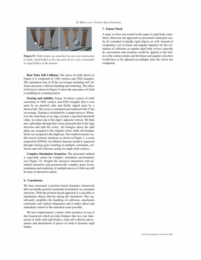
Attachments with Two Way Interaction. We can sim-ulate both, one way and two way coupled attachment con-straints. The cloth stripes in Figure 8 are attached via oneway constraints to the static rigid bodies at the top. In addi-tion, two way interaction is enabled between the stripes andthe bottom rigid bodies. This configuration results in realis-tically looking swing and twist motions of the stripes. Thescene features 6 rigid bodies and 3 pieces of cloth which aresimulated and rendered with more than 380 fps.



Figure 8: Cloth stripes are attached via one way interactionto static rigid bodies at the top and via two way constraintsto rigid bodies at the bottom.

Real Time Self Collision. The piece of cloth shown inFigure 6 is composed of 1364 vertices and 2562 triangles.The simulation runs at 30 fps on average including self col-lision detection, collision handling and rendering. The effectof friction is shown in Figure 9 where the same piece of clothis tumbling in a rotating barrel.

Tearing and stability. Figure 10 shows a piece of clothconsisting of 4264 vertices and 8262 triangles that is tornopen by an attached cube and finally ripped apart by athrown ball. This scene is simulated and rendered with 47 fpson average. Tearing is simulated by a simple process: When-ever the stretching of an edge exceeds a specified thresholdvalue, we select one of the edge’s adjacent vertices. We thenput a split plane through that vertex perpendicular to the edgedirection and split the vertex. All triangles above the splitplane are assigned to the original vertex while all trianglesbelow are assigned to the duplicate. Our method remains sta-ble even in extreme situations as shown in Figure 1, a sceneinspired by [ITF04]. An inflated character model is squeezedthrough rotating gears resulting in multiple constraints, col-lisions and self collisions acting on single cloth vertices.

Complex Simulation Scenarios. The presented methodis especially suited for complex simulation environments(see Figure 12). Despite the extensive interaction with an-imated characters and geometrically complex game levels,simulation and rendering of multiple pieces of cloth can stillbe done at interactive speed.

6. Conclusions

We have presented a position based dynamics frameworkthat can handle general constraints formulated via constraintfunctions. With the position based approach it is possible tomanipulate objects directly during the simulation. This sig-nificantly simplifies the handling of collisions, attachmentconstraints and explicit integration and it makes direct andimmediate control of the animated scene possible.

We have implemented a robust cloth simulator on top ofthis framework which provides features like two way inter-action of cloth with rigid bodies, cloth self collision and re-sponse and attachments of pieces of cloth to dynamic rigidbodies.

7. Future Work

A topic we have not treated in this paper is rigid body simu-lation. However, the approach we presented could quite eas-ily be extended to handle rigid objects as well. Instead ofcomputing a set of linear and angular impulses for the res-olution of collisions as regular rigid body solvers typicallydo, movements and rotations would be applied to the bod-ies at the contact points and the linear and angular velocitieswould have to be adjusted accordingly after the solver hascompleted.



Figure 9: Influenced by collision, self collision and friction, a piece of cloth tumbles in a rotating barrel.

Figure 10: A piece of cloth is torn open by an attached cube and ripped apart by a thrown ball.

Figure 11: Three inflated characters experience multiple collisions and self collisions.

Figure 12: Extensive interaction between pieces of cloth and an animated game character (left), a geometrically complex gamelevel (middle) and hundreds of simulated plant leaves (right).



References

[BFA02] BRIDSON R., FEDKIW R., ANDERSON J.: Robust treat-ment of collisions, contact and friction for cloth animation. Pro-ceedings of ACM Siggraph (2002), 594–603.

[BMF03] BRIDSON R., MARINO S., FEDKIW R.: Simulation ofclothing with folds and wrinkles. In ACM SIGGRAPH Sympo-sium on Computer Animation (2003), pp. 28–36.

[BW98] BARAFF D., WITKIN A.: Large steps in cloth simula-tion. Proceedings of ACM Siggraph (1998), 43–54.

[BWK03] BARAFF D., WITKIN A., KASS M.: Untangling cloth.In Proceedings of the ACM SIGGRAPH (2003), pp. 862–870.

[CBP05] CLAVET S., BEAUDOIN P., POULIN P.: Particle-basedviscoelastic fluid simulation. Proceedings of the ACM SIG-GRAPH Symposium on Computer Animation (2005), 219–228.

[DSB99] DESBRUN M., SCHRÖDER P., BARR A.: Interactiveanimation of structured deformable objects. In Proceedings ofGraphics Interface ’99 (1999), pp. 1–8.

[Fau98] FAURE F.: Interactive solid animation using linearizeddisplacement constraints. In Eurographics Workshop on Com-puter Animation and Simulation (EGCAS) (1998), pp. 61–72.

[Fed05] FEDOR M.: Fast character animation using particle dy-namics. Proceedings of International Conference on Graphics,Vision and Image Processing, GVIP05 (2005).

[GHDS03] GRINSPUN E., HIRANI A., DESBRUN M.,SCHRODER P.: Discrete shells. In Proceedings of theACM SIGGRAPH Symposium on Computer Animation (2003).

[ITF04] IRVING G., TERAN J., FEDKIW R.: Invertible finite el-ements for robust simulation of large deformation. In Proceed-ings of the ACM SIGGRAPH Symposium on Computer Animation(2004), pp. 131–140.

[Jak01] JAKOBSEN T.: Advanced character physics U the fysixengine. www.gamasutra.com (2001).

[MHTG05] MÜLLER M., HEIDELBERGER B., TESCHER M.,GROSS M.: Meshless deformations based on shape matching.Proceedings of ACM Siggraph (2005), 471–478.

[NMK∗05] NEALEN A., MÜLLER M., KEISER R., BOXERMAN

E., CARLSON M.: Physically based deformable models in com-puter graphics. Eurographics 2005 state of the art report (2005).

[Pro95] PROVOT X.: Deformation constraints in a mass-springmodel to describe rigid cloth behavior. Proceedings of GraphicsInterface (1995), 147U–154.

[Rat04] RATCLIFF J.: Rocket - a viewer for real-time phyics sim-ulations. www.physicstools.org (2004).

[THM∗03] TESCHNER M., HEIDELBERGER B., MÜLLER M.,POMERANERTS D., GROSS M.: Optimized spatial hashing forcollision detection of deformable objects. Proc. Vision, Model-ing, Visualization VMV 2003 (2003), 47–54.

[THMG04] TESCHNER M., HEIDELBERGER B., MÜLLER M.,GROSS M.: A versatile and robust model for geometrically com-plex deformable solids. Proceedings of Computer Graphics In-ternational (CGI) (2004), 312–319.

[VCMT95] VOLINO P., COURCHESNE M., MAGNENAT-THALMANN N.: Versatile and efficient techniques forsimulating cloth and other deformable objects. Proceedings ofACM Siggraph (1995), 137–144.

Appendix A:

Gradient of the Normalized Cross Product

Constraint functions often contain normalized cross products. To de-rive the projection corrections, the gradient of the constraint func-tion is needed. Therefore it is useful to know the gradient of a nor-malized cross product with respect to both arguments. Given thenormalized cross product n = p1×p2

|p1×p2 | , the derivative with respect tothe first vector is

∂n∂p1

=

∂nx∂ p1x

∂nx∂ p1y

∂nx∂ p1z

∂ny∂ p1x

∂ny∂ p1y

∂ny∂ p1z

∂nz∂ p1x

∂nz∂ p1y

∂nz∂ p1z

(16)

=1

|p1×p2|

0 p2z −p2y−p2z 0 p2xp2y −p2x 0

+n(n×p2)T

(17)

Shorter and for both arguments we have

∂n∂p1

=1

|p1×p2|(−p2 +n(n×p2)T )

(18)

∂n∂p2

=− 1|p1×p2|

(−p1 +n(n×p1)T )(19)

(20)

where p is the matrix with the property px = p×x.

Bending Constraint Projection

The constraint function for bending is C = arccos(d)−ϕ0, whered = n1 ·n2 = nT

1 n2. Without loss of generality we set p1 = 0 and getfor the normals n1 = p2×p3

|p2×p3| and n2 = p2×p4|p2×p4 | . With d

dx arccos(x) =

− 1√1−x2

we get the following gradients:

∇p3C =− 1√1−d2

((

∂n1

∂p3

)T

n2) (21)

∇p4C =− 1√1−d2

((

∂n2

∂p4

)T

n1) (22)

∇p2C =− 1√1−d2

((

∂n1

∂p2

)T

n2 +(

∂n2

∂p2

)T

n1) (23)

∇p1C =−∇p2C−∇p3C−∇p4C (24)

Using the gradients of normalized cross products, first compute

q3 =p2×n2 +(n1×p2)d

|p2×p3| (25)

q4 =p2×n1 +(n2×p2)d

|p2×p4| (26)

q2 =−p3×n2 +(n1×p3)d|p2×p3| − p4×n1 +(n2×p4)d

|p2×p4| (27)

q1 =−q2−q3−q4 (28)

Then the final correction is

∆pi =−wi√

1−d2(arccos(d)−ϕ0)∑ j w j|q j|2 qi (29)


position based dynamics - matthias...

Documents