physically-based visualization of residential building
TRANSCRIPT
University of Central Florida University of Central Florida
STARS STARS
Electronic Theses and Dissertations, 2004-2019
2007
Physically-based Visualization Of Residential Building Damage Physically-based Visualization Of Residential Building Damage
Process In Hurricane Process In Hurricane
Dezhi Liao University of Central Florida
Part of the Computer Sciences Commons
Find similar works at: https://stars.library.ucf.edu/etd
University of Central Florida Libraries http://library.ucf.edu
This Doctoral Dissertation (Open Access) is brought to you for free and open access by STARS. It has been accepted
for inclusion in Electronic Theses and Dissertations, 2004-2019 by an authorized administrator of STARS. For more
information, please contact [email protected].
STARS Citation STARS Citation Liao, Dezhi, "Physically-based Visualization Of Residential Building Damage Process In Hurricane" (2007). Electronic Theses and Dissertations, 2004-2019. 3241. https://stars.library.ucf.edu/etd/3241
PHYSICALLY-BASED VISUALIZATION OF RESIDENTIAL BUILDING DAMAGE PROCESS IN HURRICANE
by
DEZHI LIAO
B.S. National University of Defense Technology, 1993 M.S. University of Central Florida, 2006
A dissertation submitted in partial fulfillment of the requirements
for the degree of Doctor of Philosophy in Modeling and Simulation in the College of Sciences
at the University of Central Florida Orlando, Florida
Spring Term 2007
Major Professor: J. Peter Kincaid
ABSTRACT
This research provides realistic techniques to visualize the process of damage to
residential building caused by hurricane force winds. Three methods are implemented to make
the visualization useful for educating the public about mitigation measures for their homes.
First, the underline physics uses Quick Collision Response Calculation. This is an iterative
method, which can tune the accuracy and the performance to calculate collision response
between building components. Secondly, the damage process is designed as a Time-scalable
Process. By attaching a damage time tag for each building component, the visualization process
is treated as a geometry animation allowing users to navigate in the visualization. The detached
building components move in response to the wind force that is calculated using qualitative
rather than quantitative techniques. The results are acceptable for instructional systems but not
for engineering analysis. Quick Damage Prediction is achieved by using a database query instead
of using a Monte-Carlo simulation. The database is based on HAZUS® engineering analysis data
which gives it validity. A reasoning mechanism based on the definition of the overall building
damage in HAZUS® is used to determine the damage state of selected building components
including roof cover, roof sheathing, wall, openings and roof-wall connections. Exposure
settings of environmental aspects of the simulated environment, such as ocean, trees, cloud and
rain are integrated into a scene-graph based graphics engine. Based on the graphics engine and
the physics engine, a procedural modeling method is used to efficiently render residential
buildings. The resulting program, Hurricane!, is an instructional program for public education
useful in schools and museum exhibits.
ii
ACKNOWLEDGMENTS
I would like to thank my advisor, Dr. Peter Kincaid, for his continuing support and belief
in my work. My Co-Chair, Dr. Thomas Clark and Dr. David Kaup were very helpful with
mathematical aspects of this research. Dr. Forrest Master of the University of Florida provided
much needed insight relating to hurricane wind effects on buildings from the viewpoint of a civil
engineer and Dr. Zhou of UCF’s Computer Science Department provided the same kinds of
insight from the standpoint of his discipline. Mr. Glenn Martin kindly provided me with source
code from a related IST project. Mr. Jason Daly answered many technical questions about
designing the graphics engine. Dustin Chertoff, a fellow doctoral student, designed the graphical
interface for this project. Jia Luo, also a doctoral student, designed flash animations for the
tutoring modules of the Hurricane! program. Dr. Stephen Leatherman, Professor and Director of
the International Hurricane Research Center at the Florida International University, provided
funding (via NOAA and the National Hurricane Center) and encouragement for this research.
iii
TABLE OF CONTENTS
LIST OF FIGURES ....................................................................................................................... vi
LIST OF TABLES....................................................................................................................... viii
LIST OF ABBREVIATIONS........................................................................................................ ix
CHAPTER 1: INTRODUCTION .............................................................................................. 1
1.1 Background..................................................................................................................... 1
1.2 Problem Statement .......................................................................................................... 3
1.3 Research Contribution .................................................................................................... 5
1.4 Dissertation Outline ........................................................................................................ 6
CHAPTER 2: BUILDING DAMAGE VISUALIZATION SYSTEM OVERVIEW................ 7
2.1 System Interface.............................................................................................................. 7
2.2 System Structure ........................................................................................................... 17
2.3 Ocean Component......................................................................................................... 23
2.3.1 Model Selection ........................................................................................................ 23
2.3.2 Model Implementation.............................................................................................. 24
2.3.3 Result and Discussion............................................................................................... 26
2.4 Tree Simulation............................................................................................................. 28
CHAPTER 3: BUILDING STAIC MODEL ........................................................................... 29
3.1 Building Model Structure ............................................................................................. 29
3.2 Roof Model ................................................................................................................... 33
3.3 Wall and Openings Model ............................................................................................ 38
CHAPTER 4: BUILDING COMPONENT DYNAMICS....................................................... 41
4.1 Equation of Unconstrained Motion............................................................................... 43
4.2 Collision Detection ....................................................................................................... 48
4.2.1 Box-Box Collision Detection.................................................................................... 50
4.2.2 GJK Collision Detection ........................................................................................... 54
4.3 Collision Response computation................................................................................... 55
4.3.1 Constraint Analysis................................................................................................... 58
4.3.2 LCP Formulation ...................................................................................................... 61
iv
4.3.3 SOR method to solve LCP problem.......................................................................... 70
4.4 Implementation and Conclusion ................................................................................... 72
CHAPTER 5: DAMAGE PROCESS DYNAMICS ................................................................ 80
5.1 Wind Field Modeling.................................................................................................... 80
5.1.1 Upper Level Wind Model ......................................................................................... 80
5.1.2 Boundary Layer Model ............................................................................................. 84
5.2 Roof Damage Visualization.......................................................................................... 87
5.2.1 Wind Force Computation.......................................................................................... 87
5.2.2 Wind Force Coefficient............................................................................................. 89
5.2.3 Shingle and Plywood Damage Process..................................................................... 93
5.3 Wall and Opening Damage Visualization..................................................................... 98
5.4 Damage Rule Incorporation........................................................................................ 103
CHAPTER 6: CONCLUSION & FUTURE RESEARCH .................................................... 110
6.1 Conclusion .................................................................................................................. 110
6.2 Future Research .......................................................................................................... 117
REFERENCES ........................................................................................................................... 119
v
LIST OF FIGURES
Figure 1.1 Damage prediction methodology (Image courtesy of K. Gurley)................................. 4 Figure 1.2 A real-life picture of residential building with shingle loss (left) and an animation
(right) ...................................................................................................................................... 4 Figure 2.1 An example of suburban terrain in current visualization system ................................ 12 Figure 2.2 An example of open terrain used in current visualization system............................... 12 Figure 2.3 An example of a building surrounded by many trees.................................................. 13 Figure 2.4 An example of a building surrounded by few trees..................................................... 13 Figure 2.5 Peak pressure coefficients on hip roof in open terrain (Meecham, 1988)................... 15 Figure 2.6 Peak pressure coefficients on gable roof in open terrain (Meecham, 1988) ............... 15 Figure 2.7 Types of roof-wall connection: toenail (left) and strap (right).................................... 17 Figure 2.8 API hierarchy of the system ........................................................................................ 18 Figure 2.9 Framework of hurricane visualization system............................................................. 19 Figure 2.10 Key components of real-time simulation engine....................................................... 20 Figure 2.11 GraphicsManager: integration of the graphics engine and the physics engine ........ 21 Figure 2.12 Components of scene graph....................................................................................... 22 Figure 2.13 Mesh size 32 x 32 ...................................................................................................... 27 Figure 2.14 Mesh size 64 x 64 ...................................................................................................... 27 Figure 2.15 Mesh size 128 x 128 .................................................................................................. 27 Figure 3.1 Pure topological Information Struct House ................................................................. 30 Figure 3.2 Top view of gable-roof house and hip-roof house ...................................................... 31 Figure 3.3 Static diagram of component House............................................................................ 32 Figure 3.4 Roof plane grid ............................................................................................................ 35 Figure 3.5 Six different shapes of tiles on the edge of hip roof.................................................... 36 Figure 3.6 Solid shape of truss...................................................................................................... 38 Figure 3.7 Wire-frame shape of truss ........................................................................................... 38 Figure 3.8 Slab definition from [ORT96] ..................................................................................... 39 Figure 4.1 UML of BuildingComponent class and WoodWall ..................................................... 41 Figure 4.2 Center of mass and point applying force..................................................................... 44 Figure 4.3 Model of collision detection........................................................................................ 50 Figure 4.4 A touching contact (a) and a penetrating contact (b) .................................................. 58 Figure 4.5 Lagrange multiplier at contact point 1 of each iteration in test1................................. 76 Figure 4.6 Lagrange multiplier at contact point 1 and 2 in test1 .................................................. 76 Figure 4.7 Lagrange multiplier at contact point 3 and 4 in test1 .................................................. 77 Figure 4.8 Position changing with simulation step in test1 .......................................................... 77 Figure 4.9 Velocity changing with simulation step in test1.......................................................... 78 Figure 5.1 Wind speed vs. height at a location near a building .................................................... 85 Figure 5.2 Relative wind of building component ......................................................................... 88 Figure 5.3 Flow topology in the upstream (left) and downstream (right) region [BEC02].......... 89 Figure 5.4 Correlation coefficient on roof surface for cornering winds ....................................... 90 Figure 5.5 Mean pressure coefficients for cornering winds ......................................................... 90 Figure 5.6 Correlation coefficient on roof Surface for winds parallel to the ridgeline ................ 90
vi
Figure 5.7 Mean pressure coefficient for winds parallel to the ridgeline ..................................... 90 Figure 5.8 Correlation coefficient on roof surface for winds perpendicular to the ridgeline ....... 90 Figure 5.9 Mean pressure coefficients for winds perpendicular to the ridgeline.......................... 91 Figure 5.10 Mean pressure coefficient contours superimposed on gable roof framing................ 91 Figure 5.11 Mean pressure coefficient contours superimposed on hip roof framing. [UEM99].. 92 Figure 5.12 Wind angle definition ................................................................................................ 92 Figure 5.13 Definition of support mapping .................................................................................. 95 Figure 5.14 Diagram of shingle losing ......................................................................................... 97 Figure 5.15 Window with crack.................................................................................................. 102 Figure 5.16 Window break visualization using texture replacement.......................................... 102 Figure 5.17 Damage prediction diagram used by HAZUS®...................................................... 104 Figure 6.1 Iterative method with ten iterations........................................................................... 110 Figure 6.2 Iterative method with five iterations.......................................................................... 111 Figure 6.3 Shingle loss process using deterministic TOL function ............................................ 112 Figure 6.4 Shingle loss process using TOL function with some randomization ........................ 112 Figure 6.5 Gable-roof one-story house at minor damage state................................................... 114 Figure 6.6 Gable-roof one-story house at severe damage state .................................................. 114 Figure 6.7 Gable-roof two-story house at severe damage state .................................................. 115 Figure 6.8 Hip-roof two-story house at severe damage state viewing from windward.............. 115 Figure 6.9 Hip-roof two-story house at severe damage state viewing from leeward ................. 116 Figure 6.10 Hip-roof one-story house at destruction state.......................................................... 116 Figure 6.11 Visualizing damage process of multiple residential buildings in a hurricane event 118
vii
LIST OF TABLES
Table 2.1 Hurricane category and its effect .................................................................................... 8 Table 2.2 Surface roughness of different types of terrain defined in HAZUS® .......................... 10 Table 2.3 Parameter of Phillips spectrum..................................................................................... 24 Table 2.4 Parameters in equation (2.2) and their definition ......................................................... 25 Table 3.1 Out-code definition in CSLC algorithm ....................................................................... 37 Table 4.1 Separating axis test of box-box collision for different contact types ........................... 53 Table 4.2 Values for test 1 ............................................................................................................ 75 Table 5.1 Wind force scale coefficients........................................................................................ 93 Table 5.2 Maximum TOLS and minimum TOLS indexing table................................................. 96 Table 5.3 Damage state for residential buildings defined in HAZUS® ..................................... 105 Table 5.4 Tabulated Venn diagram............................................................................................. 108
viii
LIST OF ABBREVIATIONS
API Application Program Interface
CBD Component-based Development
CBSE Component-based Software Engineering
CPU Computer Processor Unit
CSLC Cohen-Sutherland Line-Clipping algorithm
FCMP Florida Coastal Monitoring Program
FHA Florida Hurricane Alliance
GJK Gilbert-Johnson-Keerthi
HLRP Hurricane Loss Reduction Project
IST Institute for Simulation & Training
LCP Linear Complementarity Problem
MPH Miles per Hour
ODE Ordinary Differential Equation
OSB Oriented Strand Board
PBL Planetary Boundary Layer
TOL Time of Lost
SOR Successive Over Relaxation
UML Unified Modeling Language
ix
CHAPTER 1: INTRODUCTION
1.1 Background
In a recent yearly progress report on the Florida Hurricane Alliance (FHA), Leatherman
(2005) provides a persuasive case for hurricane research to improve our response to hurricanes
and to prepare for them [LEA05]:
“Extreme hurricane events in recent years have, with an increasing sense of urgency,
reinforced the proposition that the nation must continue to work on, but also move
beyond weather prediction and evacuation to achieve significant damage reduction.
Against this background, increasing population and urban development in coastal areas
highlight the dynamic nature of our vulnerability to hurricanes and the urgency of the
problem.”
The Florida Hurricane Alliance (FHA), the sponsor of the research reported in this
dissertation, has done much to develop techniques for mitigating hurricane damage. Techniques
to achieve this have included data collection, social and behavioral research, communication
technology, computer modeling, simulation and visualization (the technique used in this
dissertation project). The FHA is a multidisciplinary cooperative research effort, which brings
together capabilities and evolving expertise of the public universities in Florida to focus on
hurricane loss reduction. Public education regarding hurricane effects on residential buildings
and mitigation techniques is one of the missions of the FHA, which this dissertation addresses.
Much research relating to hurricane damage mitigation has already been conducted. For
example, the Hurricane Loss Reduction Project, conducted by research teams from Clemson
University, Virginia Polytechnic Institute and State University, the University of Illinois at
1
Urbana-Champaign, Johns Hopkins University and the University of Florida, aims to strengthen
the relevant scientific and engineering base [POW03], [COP04]. This program has included a
coordinated series of research activities in areas like wind load magnitudes, wind characteristics,
physical modeling and simulation of structural capacities, simulation and modeling tools for
database-assisted, reliability-based design. The Florida Coastal Monitoring Program (FCMP) is
another unique joint venture conducting full-scale experiment to quantify near-surface hurricane
wind behavior and the resultant loads on residential structures [MAS03]. The FCMP aims to
provide the data necessary for identifying methods to cost-effectively reduce hurricane wind
damage to residential structures. FCMP is a contribution to improve the understanding of ground
level hurricane winds and to develop the ability to simulate wind loading on low-rise structures
in hurricane prone regions. In addition, the State of Florida Department of Insurance sponsors the
development of an open catastrophic loss model to assess the risk to insured residential property
due to damaging hurricane winds. This model allows for user input at all stages in order to
examine various risk scenarios. Using a component approach, its Monte Carlo Simulation engine
generates damage information for typical Florida homes and compares deterministic wind loads
with the probabilistic capacity of vulnerable building components to determine the probability of
damage.
In the wake of hurricane Katrina, data on damage to wood-frame residential structures
along the U.S. Gulf Coast was collected under the direction of J. van de Lindt of Colorado State
University [LIN05]. Residential buildings damage caused by hurricane Katrina shows that even
small violations of building code can result in great damage. The general public tends not to
understand building codes, that are mainly based on complicated engineering data and
2
meteorology. It is important to make hurricane damage and mitigation measures understandable
to the general public. Previous hurricane visualization projects [WAT04], mostly focused on the
macroscopic impact of hurricanes. A visualization system shows what happened in detail and is
useful for educating the general public knowledge about hurricane mitigation measures.
Research shows that interactive simulation has a much more intuitive educational effect than a
passive video [BOS88], [NET88], [FLE90] and [MUL92]. As a member of FHA, the University
of Central Florida was tasked to develop an interactive simulation application for wind damage
visualization to include a variety of structures and environmental conditions. The development of
procedures and algorithms for automating and facilitating the creation of these visualizations
were seen as necessary.
1.2 Problem Statement
The goal of this research is to realistically depict hurricane damage to typical residential
buildings using an interactive simulation. To ensure the validity of the visualization, we use
engineering analysis results (hurricane damage predictions), as an input to the visualization
engine. However, the output is only an approximation of what would be achieved by
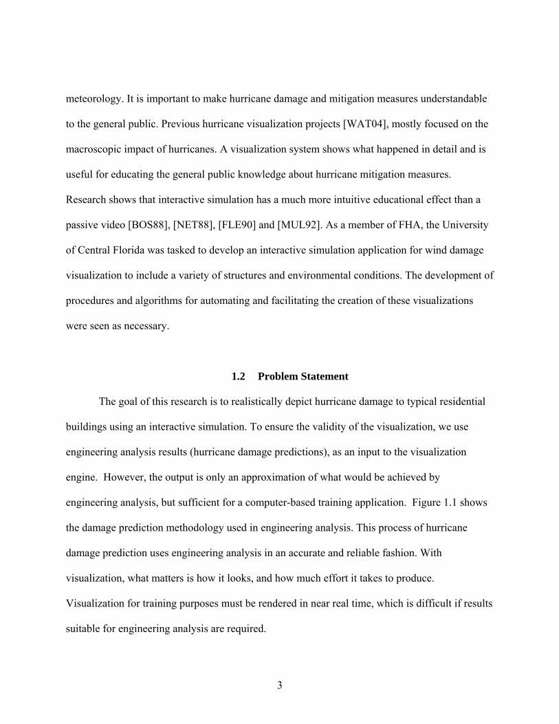
engineering analysis, but sufficient for a computer-based training application. Figure 1.1 shows
the damage prediction methodology used in engineering analysis. This process of hurricane
damage prediction uses engineering analysis in an accurate and reliable fashion. With
visualization, what matters is how it looks, and how much effort it takes to produce.
Visualization for training purposes must be rendered in near real time, which is difficult if results
suitable for engineering analysis are required.
3
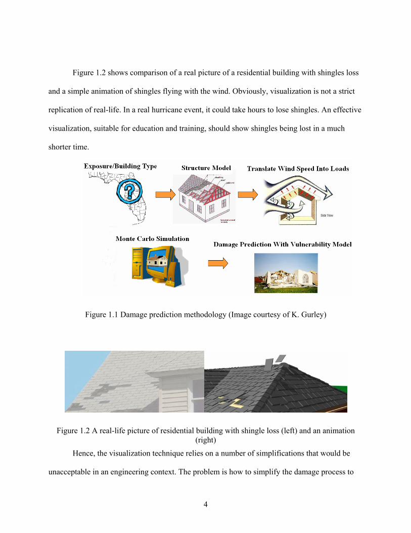
Figure 1.2 shows comparison of a real picture of a residential building with shingles loss
and a simple animation of shingles flying with the wind. Obviously, visualization is not a strict
replication of real-life. In a real hurricane event, it could take hours to lose shingles. An effective
visualization, suitable for education and training, should show shingles being lost in a much
shorter time.
Figure 1.1 Damage prediction methodology (Image courtesy of K. Gurley)
Figure 1.2 A real-life picture of residential building with shingle loss (left) and an animation (right)
Hence, the visualization technique relies on a number of simplifications that would be
unacceptable in an engineering context. The problem is how to simplify the damage process to
4

make the visualization understandable by the general public yet maintain enough engineering
realism for educational purposes.
1.3 Research Contribution
The first research contribution is the development of a solid framework with graphics and
physics engines to visualize the residential building damage process. The user defines both the
residential building and the hurricane event. Interactivity between the program and the user
typically makes for compelling instruction; it supports the process of “learn by doing”.
The second research contribution is to achieve an acceptable visual update frame-rate
without over-simplifying the visualization to the point that it loses its realism. We implemented
three methods.
1) Quick Collision Response Calculation. An iterative method is used to calculate
collision response among building components. This results in objects
converging in a realistic way based on preset thresholds.
2) Time-scalable Damage Process Visualization. The damage process visualization
is treated as a geometry animation by attaching a damage time tag for each
building component. Detached building components are allowed to move in
response to the wind force that is calculated using qualitative rather than
quantitative techniques. The results are acceptable for educational purposes but
not for engineering analysis.
5
3) Quick Damage Prediction. We use a database query for damage prediction
instead of using a Monte-Carlo simulation. The database is currently based on
HAZUS® software. However, its flexible structure allows easy modification.
Based on the graphics engine and the physics engine, a procedural modeling method is
used to model the residential building. Compared to the traditional way of modeling buildings
offline, this method saves many hours of artists’ work. Use of the procedural modeling method
also allows visualizing damage to multiple buildings during a hurricane event.
1.4 Dissertation Outline
The remainder of this document is organized as follows: Chapter 2 presents the overview
design of the hurricane visualization system and the graphics engine. Chapter 3 describes the
residential building static model. Chapter 4 describes the physics engine used in this research.
Chapter 5 discusses the dynamic residential building model based on engineering analysis results
relating to hurricane damage. Chapter 6 presents conclusions and recommendations for future
research. Component-based software engineering (CBSE) is used in the system design and
implementation. Unified modeling language (UML) is used to depict each component in detail.
6
CHAPTER 2: BUILDING DAMAGE VISUALIZATION SYSTEM OVERVIEW
This chapter gives an overview analysis and design of the system interface and the real-
time simulation engine. Following the component-based software engineering (CBSE) method, a
mix of bottom-up and top-down design approaches are used.
2.1 System Interface
System inputs consist of data relating to the surrounding terraine (the exposure setting)
and the components of the building (building structure setting). The visualization system
database structure is based on building damage data drawn from HAZUS®. The exposure
definition includes incident wind, terrain type and amount of trees surrounding the building.
Wind speed used in HAZUS® ranges from 50 to 250 miles per hour (shown at 5 mph
intervals). Table 2.1 shows the six categories wind speeds according to the Saffir-Simpson scale,
along with a description of typical damage for each category.
7
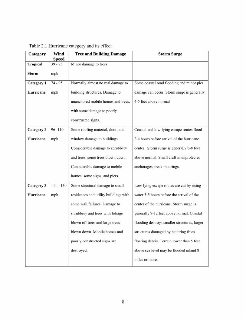
Table 2.1 Hurricane category and its effect
Category Wind Speed
Tree and Building Damage Storm Surge
Tropical
Storm
39 - 73
mph
Minor damage to trees
Category 1
Hurricane
74 - 95
mph
Normally almost no real damage to
building structures. Damage to
unanchored mobile homes and trees,
with some damage to poorly
constructed signs.
Some coastal road flooding and minor pier
damage can occur. Storm surge is generally
4-5 feet above normal
Category 2
Hurricane
96 -110
mph
Some roofing material, door, and
window damage to buildings.
Considerable damage to shrubbery
and trees, some trees blown down.
Considerable damage to mobile
homes, some signs, and piers.
Coastal and low-lying escape routes flood
2-4 hours before arrival of the hurricane
center. Storm surge is generally 6-8 feet
above normal. Small craft in unprotected
anchorages break moorings.
Category 3
Hurricane
111 - 130
mph
Some structural damage to small
residences and utility buildings with
some wall failures. Damage to
shrubbery and trees with foliage
blown off trees and large trees
blown down. Mobile homes and
poorly constructed signs are
destroyed.
Low-lying escape routes are cut by rising
water 3-5 hours before the arrival of the
center of the hurricane. Storm surge is
generally 9-12 feet above normal. Coastal
flooding destroys smaller structures, larger
structures damaged by battering from
floating debris. Terrain lower than 5 feet
above sea level may be flooded inland 8
miles or more.
8
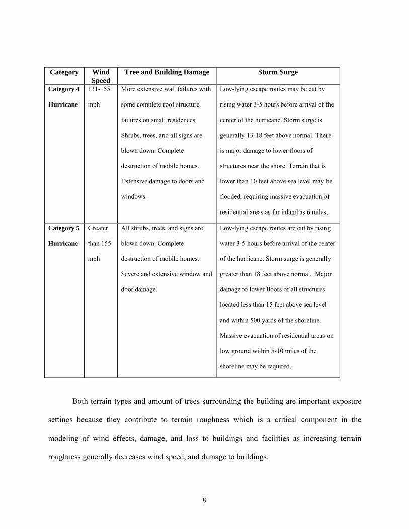
Category Wind Speed
Tree and Building Damage Storm Surge
Category 4
Hurricane
131-155
mph
More extensive wall failures with
some complete roof structure
failures on small residences.
Shrubs, trees, and all signs are
blown down. Complete
destruction of mobile homes.
Extensive damage to doors and
windows.
Low-lying escape routes may be cut by
rising water 3-5 hours before arrival of the
center of the hurricane. Storm surge is
generally 13-18 feet above normal. There
is major damage to lower floors of
structures near the shore. Terrain that is
lower than 10 feet above sea level may be
flooded, requiring massive evacuation of
residential areas as far inland as 6 miles.
Category 5
Hurricane
Greater
than 155
mph
All shrubs, trees, and signs are
blown down. Complete
destruction of mobile homes.
Severe and extensive window and
door damage.
Low-lying escape routes are cut by rising
water 3-5 hours before arrival of the center
of the hurricane. Storm surge is generally
greater than 18 feet above normal. Major
damage to lower floors of all structures
located less than 15 feet above sea level
and within 500 yards of the shoreline.
Massive evacuation of residential areas on
low ground within 5-10 miles of the
shoreline may be required.
Both terrain types and amount of trees surrounding the building are important exposure
settings because they contribute to terrain roughness which is a critical component in the
modeling of wind effects, damage, and loss to buildings and facilities as increasing terrain
roughness generally decreases wind speed, and damage to buildings.
9
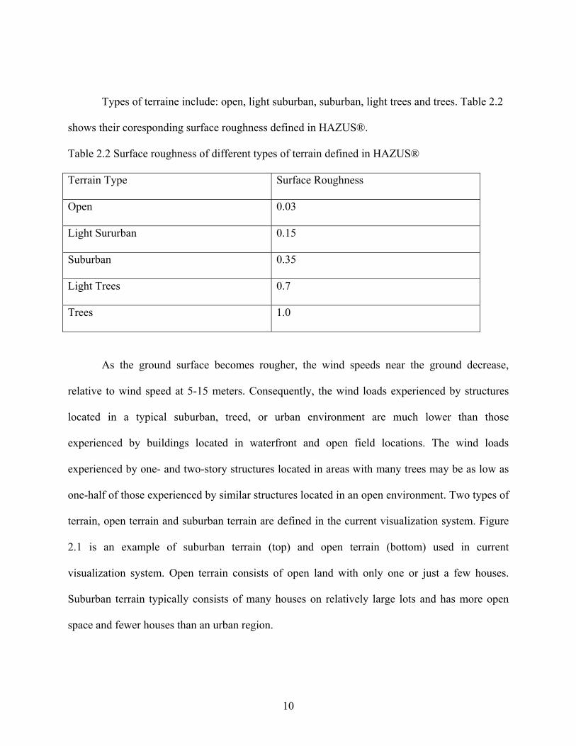
Types of terraine include: open, light suburban, suburban, light trees and trees. Table 2.2
shows their coresponding surface roughness defined in HAZUS®.
Table 2.2 Surface roughness of different types of terrain defined in HAZUS®
Terrain Type Surface Roughness
Open 0.03
Light Sururban 0.15
Suburban 0.35
Light Trees 0.7
Trees 1.0
As the ground surface becomes rougher, the wind speeds near the ground decrease,
relative to wind speed at 5-15 meters. Consequently, the wind loads experienced by structures
located in a typical suburban, treed, or urban environment are much lower than those
experienced by buildings located in waterfront and open field locations. The wind loads
experienced by one- and two-story structures located in areas with many trees may be as low as
one-half of those experienced by similar structures located in an open environment. Two types of
terrain, open terrain and suburban terrain are defined in the current visualization system. Figure
2.1 is an example of suburban terrain (top) and open terrain (bottom) used in current
visualization system. Open terrain consists of open land with only one or just a few houses.
Suburban terrain typically consists of many houses on relatively large lots and has more open
space and fewer houses than an urban region.
10
Three types of trees amounts are: no trees, few trees and many trees. A house with a few
trees around it is less likely to be damaged by a hurricane than a house with no trees (assuming a
tree is not blown down onto the house. Proper pruning tips should be followed. A house with
many trees around it is even less likely to be damaged by a hurricane providing that the correct
variety of trees are selected and planted at least 30 feet from the house.
11
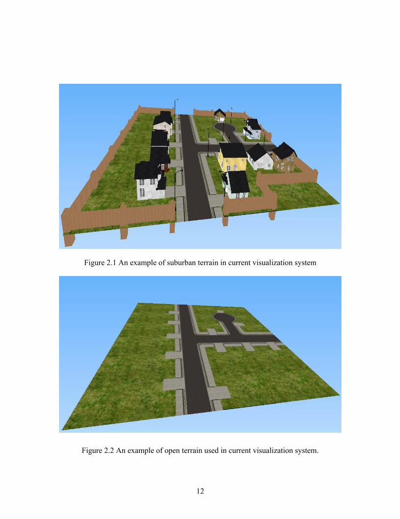
Figure 2.1 An example of suburban terrain in current visualization system
Figure 2.2 An example of open terrain used in current visualization system.
12
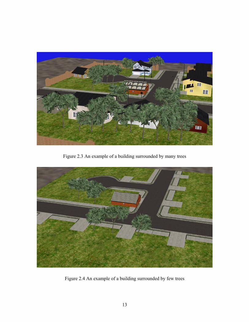
Figure 2.3 An example of a building surrounded by many trees
Figure 2.4 An example of a building surrounded by few trees
13
Types of building in HAZUS® are complicated. They are combinations of general
building types, roof types, roof-deck attachment method, roof-wall connection methods, number
of stories and four mitigation measures.
General building types are categorized according to basic construction: e.g., wood frame,
masonry, concrete, steel or manufactured home. Our visualization sytem currently includes only
two types: mansonry and wooden houses. Normally a wooden house is less resistant to wind than
a masonry house
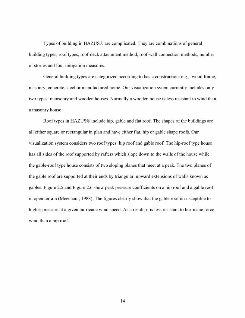
Roof types in HAZUS® include hip, gable and flat roof. The shapes of the buildings are
all either square or rectangular in plan and have either flat, hip or gable shape roofs. Our
visualization system considers two roof types: hip roof and gable roof. The hip-roof type house
has all sides of the roof supported by rafters which slope down to the walls of the house while
the gable-roof type house consists of two sloping planes that meet at a peak. The two planes of
the gable roof are supported at their ends by triangular, upward extensions of walls known as
gables. Figure 2.5 and Figure 2.6 show peak pressure coefficients on a hip roof and a gable roof
in open terrain (Meecham, 1988). The figures clearly show that the gable roof is susceptible to
higher pressure at a given hurricane wind speed. As a result, it is less resistant to hurricane force
wind than a hip roof.
14
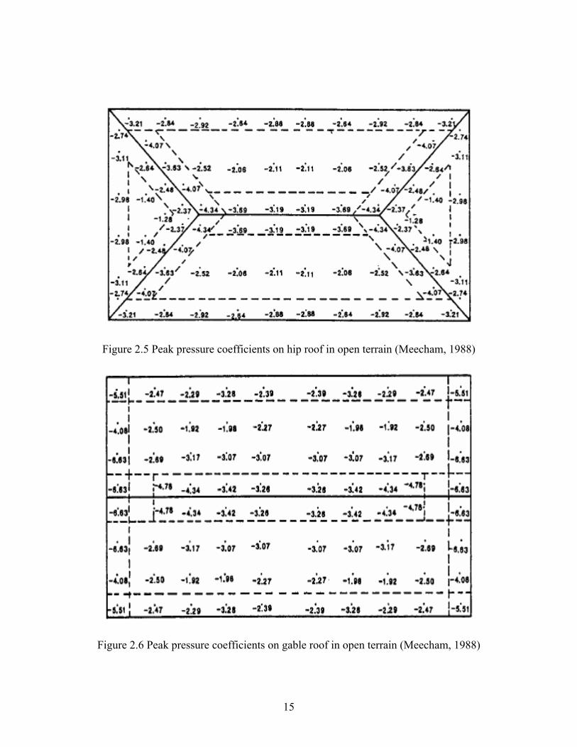
Figure 2.5 Peak pressure coefficients on hip roof in open terrain (Meecham, 1988)
Figure 2.6 Peak pressure coefficients on gable roof in open terrain (Meecham, 1988)
15

There are serveral types of roof-deck attachment methods defined in HAZUS®. Typical
types include:
1) 6d Nails @ 6/12” uses 2 inches long nails spaced at 6 inches along the edge of the
sheathing and 12 inches in the interior of the sheathing.
2) 8d Nails @6/12” differs only in its use of 2.5 inches long nails.
3) 8d Nails @6/6” uses 2.5 inches long nails on both the edge of the sheathing and
the interior of the sheathing. This connection pattern is seen mostly in newer
homes built to high wind standards.
The roof wall connection refers to how the trusses are anchored to the wall to resist the
upward force that strong winds can sometimes exert on the roof. HAZUS® defines whole roof
failure as a relatively simple model, where the roof is considered to fail as a complete unit if the
wind induced uplift loads exceed the total resistance of the roof provided by the roof-wall
connections and the the weight of the roof. In the case of gable roofs, roof trusses are assumed to
be spaced at 24” on center along two walls of the building. In the case of hip roofs, a roof-wall
connection is assumed to exist at 24” intervals along the entire perimeter of the building (i.e., for
a square building, the hip roof has twice as many roof-wall connections as the gable roof). Two
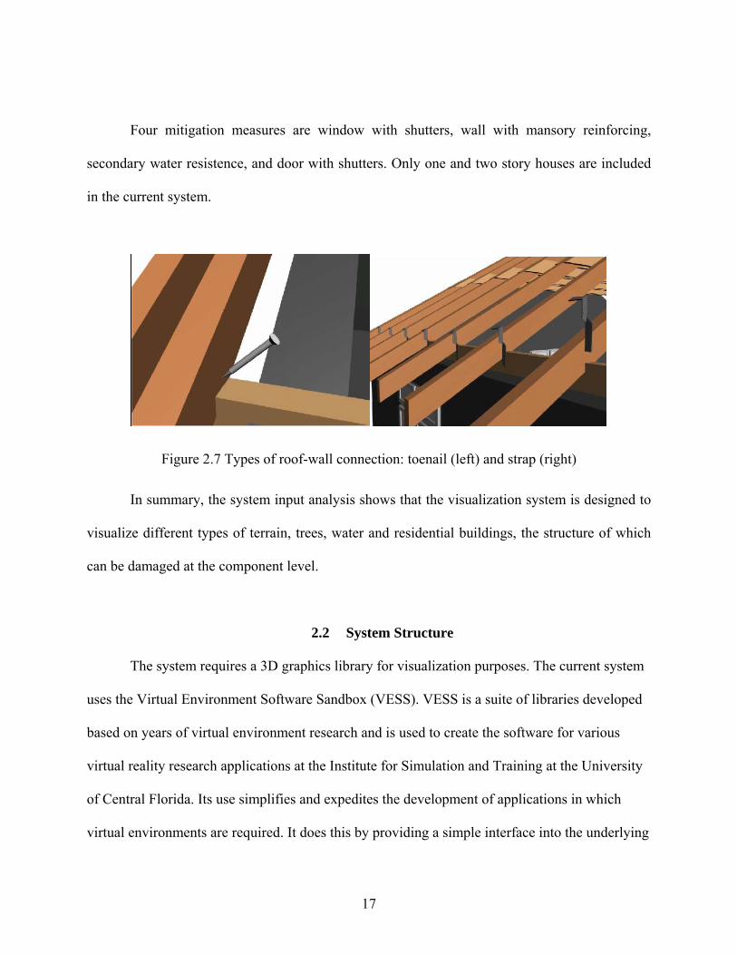
types of roof-wall connection are used in our visualization system setting: toe nails and straps.
Toe nails are nails or screws that are driven at an angle through the truss into the top plate of the
wall as is shown as Figure 2.7 (left). Straps are wrapped over the top of the truss and attached to
the wall on the same side as the truss as shown as Figure 2.7 (right).
16
Four mitigation measures are window with shutters, wall with mansory reinforcing,
secondary water resistence, and door with shutters. Only one and two story houses are included
in the current system.
Figure 2.7 Types of roof-wall connection: toenail (left) and strap (right)
In summary, the system input analysis shows that the visualization system is designed to
visualize different types of terrain, trees, water and residential buildings, the structure of which
can be damaged at the component level.
2.2 System Structure
The system requires a 3D graphics library for visualization purposes. The current system
uses the Virtual Environment Software Sandbox (VESS). VESS is a suite of libraries developed
based on years of virtual environment research and is used to create the software for various
virtual reality research applications at the Institute for Simulation and Training at the University
of Central Florida. Its use simplifies and expedites the development of applications in which
virtual environments are required. It does this by providing a simple interface into the underlying
17
graphics API, while integrating support for various input devices, such as joysticks and motion
tracking systems, and display devices, such as head-mounted displays and shutter glasses.
Additionally, VESS provides behaviors and motion models to allow the user to manipulate his or
her viewpoint as well as control and interact with objects in the virtual environment. Such
features have enabled VESS to evolve into a virtual reality system and enhance its utility for use
with educational software. VESS itself has been developed using CBD methods. The version of
VESS used in the current research utilizes components from OpenScenegraph, a scene graph
based rendering engine. OpenScenegraph is built using OpenGL API. Using VESS frees the
developer from implementing and optimizing low-level graphics calls, and provides many
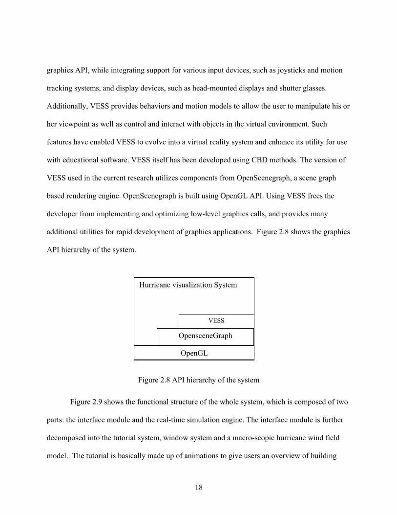
additional utilities for rapid development of graphics applications. Figure 2.8 shows the graphics
API hierarchy of the system.
Hurricane visualization System
VESS
OpensceneGraph
OpenGL
Figure 2.8 API hierarchy of the system
Figure 2.9 shows the functional structure of the whole system, which is composed of two
parts: the interface module and the real-time simulation engine. The interface module is further
decomposed into the tutorial system, window system and a macro-scopic hurricane wind field
model. The tutorial is basically made up of animations to give users an overview of building
18
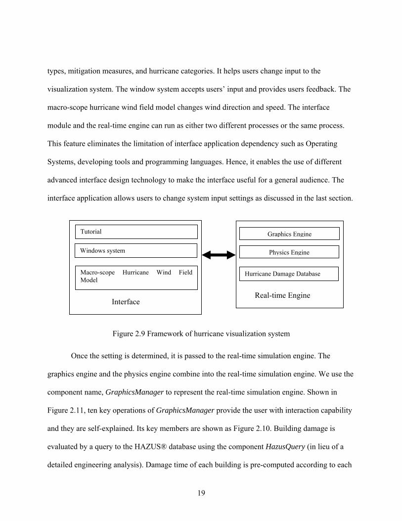
types, mitigation measures, and hurricane categories. It helps users change input to the
visualization system. The window system accepts users’ input and provides users feedback. The
macro-scope hurricane wind field model changes wind direction and speed. The interface
module and the real-time engine can run as either two different processes or the same process.
This feature eliminates the limitation of interface application dependency such as Operating
Systems, developing tools and programming languages. Hence, it enables the use of different
advanced interface design technology to make the interface useful for a general audience. The
interface application allows users to change system input settings as discussed in the last section.
Graphics Engine Tutorial
Macro-scope Hurricane Wind Field Model
Physics Engine
Interface Real-time Engine
Hurricane Damage Database
Windows system
Figure 2.9 Framework of hurricane visualization system
Once the setting is determined, it is passed to the real-time simulation engine. The
graphics engine and the physics engine combine into the real-time simulation engine. We use the
component name, GraphicsManager to represent the real-time simulation engine. Shown in
Figure 2.11, ten key operations of GraphicsManager provide the user with interaction capability
and they are self-explained. Its key members are shown as Figure 2.10. Building damage is
evaluated by a query to the HAZUS® database using the component HazusQuery (in lieu of a
detailed engineering analysis). Damage time of each building is pre-computed according to each
19
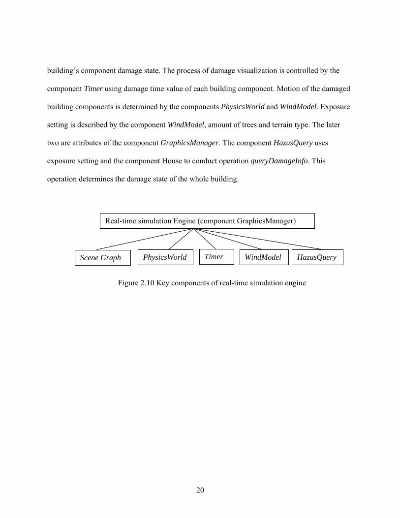
building’s component damage state. The process of damage visualization is controlled by the
component Timer using damage time value of each building component. Motion of the damaged
building components is determined by the components PhysicsWorld and WindModel. Exposure
setting is described by the component WindModel, amount of trees and terrain type. The later
two are attributes of the component GraphicsManager. The component HazusQuery uses
exposure setting and the component House to conduct operation queryDamageInfo. This
operation determines the damage state of the whole building.
Scene Graph PhysicsWorld
Real-time simulation Engine (component GraphicsManager)
Timer WindModel HazusQuery
Figure 2.10 Key components of real-time simulation engine
20
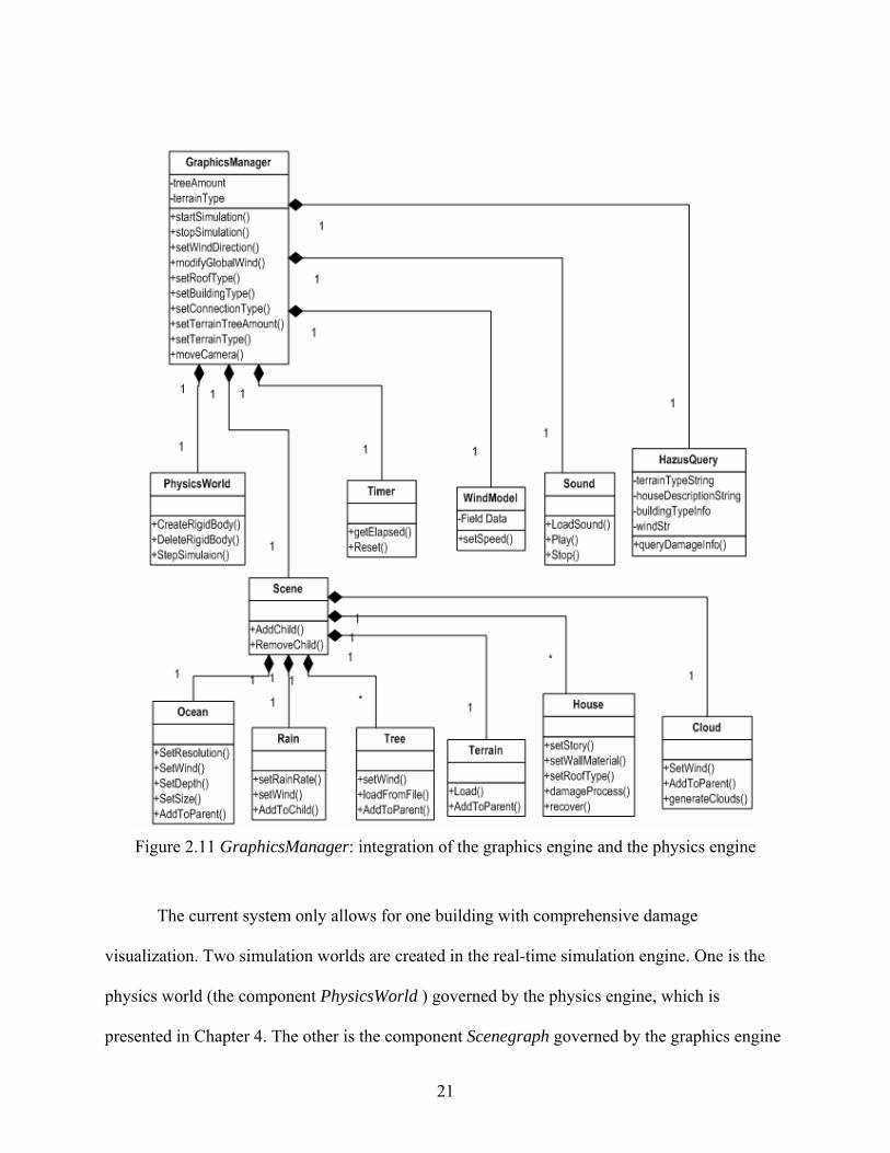
Figure 2.11 GraphicsManager: integration of the graphics engine and the physics engine
The current system only allows for one building with comprehensive damage
visualization. Two simulation worlds are created in the real-time simulation engine. One is the
physics world (the component PhysicsWorld ) governed by the physics engine, which is
presented in Chapter 4. The other is the component Scenegraph governed by the graphics engine
21
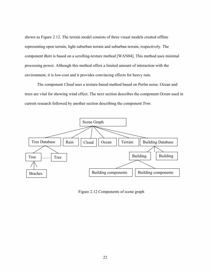
shown as Figure 2.12. The terrain model consists of three visual models created offline
representing open terrain, light suburban terrain and suburban terrain, respectively. The
component Rain is based on a scrolling-texture method [WAN04]. This method uses minimal
processing power. Although this method offers a limited amount of interaction with the
environment, it is low-cost and it provides convincing effects for heavy rain.
The component Cloud uses a texture-based method based on Perlin noise. Ocean and
trees are vital for showing wind effect. The next section describes the component Ocean used in
current research followed by another section describing the component Tree.
Scene Graph
Rain Tree Database Building Database
Tree Tree …….
Terrain Cloud Ocean
Braches
Building Building
Building components ……. Building components
Figure 2.12 Components of scene graph
22
2.3 Ocean Component
2.3.1 Model Selection
An “ideal” ocean wave model for hurricane visualization would have the following
features. It would represent different sea states ranging from calm to stormy conditions with the
appropriate response to winds of various speeds. It would interact with the seabed to generate
surf, spray and wave refraction. Finally, it would provide physical information such as speed,
pressure effects on vessels, and pressure effects on off-shore and coastal structures.
The Navier-Stokes model provides visual and physical information such as velocities and
forces. Since it is computationally intensive, it requires “simplification” for our purposes. The
Gerstner wave formulas use a sum of weighted sinusoids as exact solutions of the equations of
motion for a homogeneous incompressible fluid with a free surface. The realism of this model is
limited by difficulties of picking weight coefficients of sinusoids and it provides no physical
information, let alone wind response.
The ocean wave model in the current research is spectrum-based. This model is also
based on the theory that wave height field can be decomposed to a sum of sinusoids and cosines.
A spectrum-based ocean model is used for the following reasons:
1) It enables a seamless large water surface generation in real-time.
2) Most importantly, it has wind response.
3) The fast Fourier transforms (FFT) and the inverse FFT (IFFT) allow us to quickly solve
the equations on a standard PC.
23
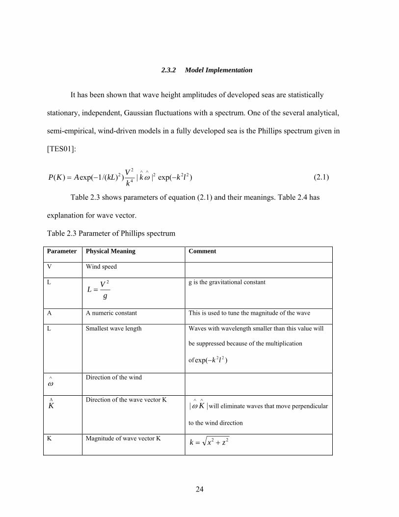
2.3.2 Model Implementation
It has been shown that wave height amplitudes of developed seas are statistically
stationary, independent, Gaussian fluctuations with a spectrum. One of the several analytical,
semi-empirical, wind-driven models in a fully developed sea is the Phillips spectrum given in
[TES01]:
)exp(||))/(1exp()( 2224
22 lkk
kVkLAKP −−=
∧∧
ω (2.1)
Table 2.3 shows parameters of equation (2.1) and their meanings. Table 2.4 has
explanation for wave vector.
Table 2.3 Parameter of Phillips spectrum
Parameter Physical Meaning Comment
V Wind speed
L
gVL
2
= g is the gravitational constant
A A numeric constant This is used to tune the magnitude of the wave
L Smallest wave length Waves with wavelength smaller than this value will
be suppressed because of the multiplication
of )exp( 22lk−
∧
ω Direction of the wind
Λ
K Direction of the wave vector K
|will eliminate waves that move perpendicular
to the wind direction
|∧∧
Kω
K Magnitude of wave vector K 22 zxk +=
24
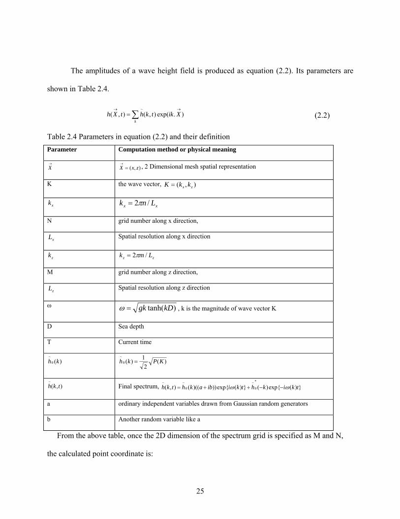
The amplitudes of a wave height field is produced as equation (2.2). Its parameters are
shown in Table 2.4.
∑→→
=k
XiktkhtXh ).exp(),(),(~
(2.2)
Table 2.4 Parameters in equation (2.2) and their definition Parameter Computation method or physical meaning
),( zxX =→ , 2 Dimensional mesh spatial representation →
X
K the wave vector, ),( zx kkK =
xx Lnk /2π= xk
N grid number along x direction,
Spatial resolution along x direction xL
zk zz Lmk /2π=
M grid number along z direction,
Spatial resolution along z direction zL
ω )tanh(kDgk=ω , k is the magnitude of wave vector K
D Sea depth
T Current time
)(2
1)(0
~KPkh = )(0
~kh
Final spectrum, })(exp{)(})(exp{)))(((),(*
0
~
0
~~tkikhtkiibakhtkh ωω −−++=),(
~tkh
a ordinary independent variables drawn from Gaussian random generators
b Another random variable like a
From the above table, once the 2D dimension of the spectrum grid is specified as M and N,
the calculated point coordinate is:
25
NnLx x /= , , MmLz z /= ),( tXhy→
=
To calculate the light response for visualization purpose, the normal of the wave surface is
computed as equation (2.3).
∑→→
=∇=k
XiktkhiktxhtXn ).exp(),(),(),(~ (2.3)
To integrate the Ocean component into the SceneGraph component, we set a callback
process for the component Ocean so that the render operation of the SceneGraph component will
call the render operation of the Ocean component automatically.
Key operations of component Ocean are initialization, setWind , update, and render. The
initialization operation generates random numbers. The setWind operation take wind speed
magnitude and direction to compute spectrum P(k), Fourier amplitude h0(k). The update
operation calculates the final spectrum and conducts a Inverse Fourier Transform (IFT) on
to get the height field . Thus, only with wind speed change, will the Fourier
amplitude h
),(~
tkh
),(~
tkh ),( tXh→
0(k) e recalculated.
In the current research, only the real part of final spectrum is used. Therefore, only the real
part of the Fourier amplitude is calculated as equation (2.4).
))sin()cos()((),( 0
~~tbtakhtkh ωω −= (2.4)
2.3.3 Result and Discussion
A key assumption of spectrum-based ocean wave model is that the ocean surface is a
mesh with a regular grid size. The vertices of the mesh are mapped to a height field generated by
applying an Inverse Fast Fourier Transformation (IFFT) to the spectrum data. The number of
26
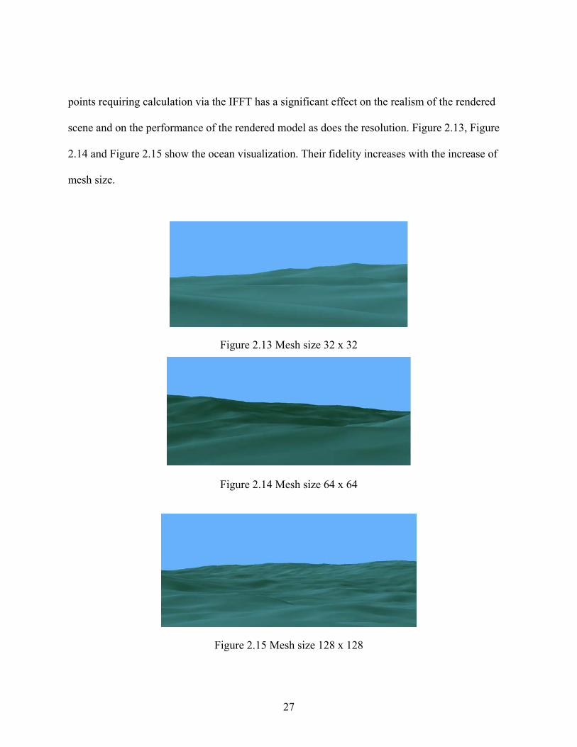
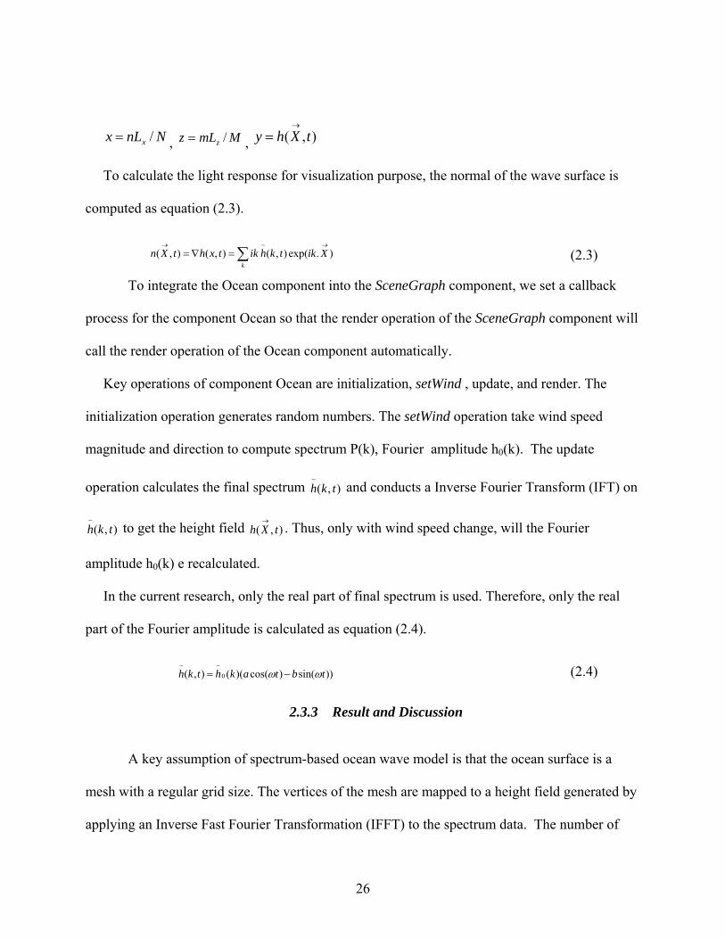
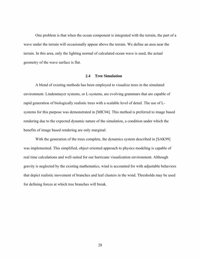
points requiring calculation via the IFFT has a significant effect on the realism of the rendered
scene and on the performance of the rendered model as does the resolution. Figure 2.13, Figure
2.14 and Figure 2.15 show the ocean visualization. Their fidelity increases with the increase of
mesh size.
Figure 2.13 Mesh size 32 x 32
Figure 2.14 Mesh size 64 x 64
Figure 2.15 Mesh size 128 x 128
27
One problem is that when the ocean component is integrated with the terrain, the part of a
wave under the terrain will occasionally appear above the terrain. We define an area near the
terrain. In this area, only the lighting normal of calculated ocean wave is used, the actual
geometry of the wave surface is flat.
2.4 Tree Simulation
A blend of existing methods has been employed to visualize trees in the simulated
environment. Lindenmayer systems, or L-systems, are evolving grammars that are capable of
rapid generation of biologically realistic trees with a scalable level of detail. The use of L-
systems for this purpose was demonstrated in [MIC04]. This method is preferred to image based
rendering due to the expected dynamic nature of the simulation, a condition under which the
benefits of image based rendering are only marginal.
With the generation of the trees complete, the dynamics system described in [SAK99]
was implemented. This simplified, object oriented approach to physics modeling is capable of
real time calculations and well suited for our hurricane visualization environment. Although
gravity is neglected by the existing mathematics, wind is accounted for with adjustable behaviors
that depict realistic movement of branches and leaf clusters in the wind. Thresholds may be used
for defining forces at which tree branches will break.
28
CHAPTER 3: BUILDING STAIC MODEL
Each structure setting change causes the change to the graphical model of the building.
To avoid building many graphical models for different types of building, procedural modeling
method is used to generate geometry of a building by just specify topology information. This
chapter treats the problem of how to design this topology information and how to generate
geometry of the whole building and position, orientation of shingles, plywood, bricks
automatically.
3.1 Building Model Structure
A little field investigation shows a residential building includes a foundation
construction, a wall construction and a roof construction. Roof construction is the most
complicated process. Normally, it consists of a roof frame, attached sheathing (typically
plywood), felt paper and roof shingles. For example, a gable roof frame is constructed using
rafters, ridge board and trusses. Since the goal of modeling the residential building if for
visualizing the damage process, we decompose the building following concept of [PIN04], i.e.
the building model is composed of a: roof cover model, roof sheathing model, wall model, roof-
wall connection model and opening model. We limit our roof cover to shingles, and limit our
sheathing to plywood.
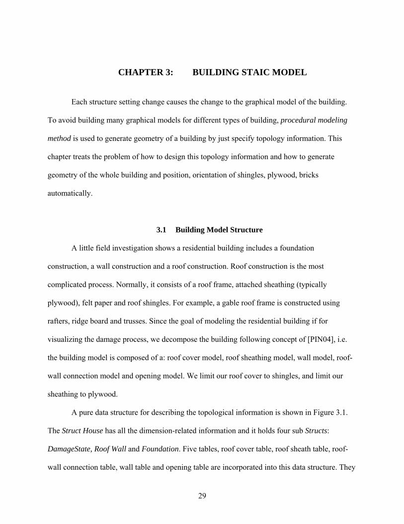
A pure data structure for describing the topological information is shown in Figure 3.1.
The Struct House has all the dimension-related information and it holds four sub Structs:
DamageState, Roof Wall and Foundation. Five tables, roof cover table, roof sheath table, roof-
wall connection table, wall table and opening table are incorporated into this data structure. They
29
serve as interpolation tables for building components to determine their damage states. Five
Boolean values show whether building components are damaged or not. They are leveraged for
implementing damage rules in Chapter 5.
Figure 3.1 Pure topological Information Struct House
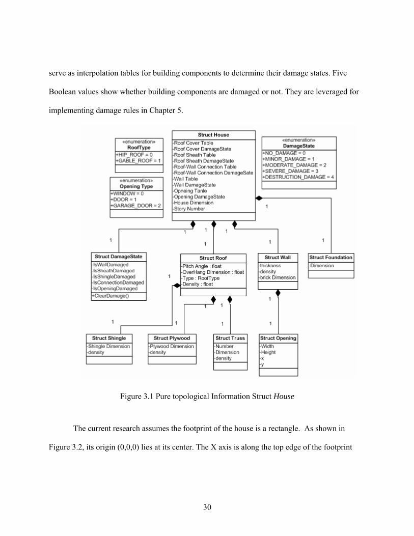
The current research assumes the footprint of the house is a rectangle. As shown in
Figure 3.2, its origin (0,0,0) lies at its center. The X axis is along the top edge of the footprint
30
with right direction as positive. The Y axis is along the right edge of the footprint with upside
direction as positive.
Y
House Foot Print Overhang Y
Hip Roof
Y
House Foot Print O
verhang Y
Gable Roof
Overhang X
X
Overhang X
X
Figure 3.2 Top view of gable-roof house and hip-roof house
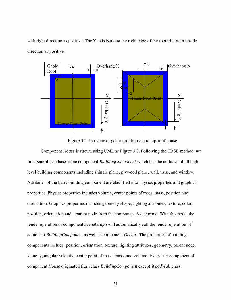
Component House is shown using UML as Figure 3.3. Following the CBSE method, we
first generilize a base-stone component BuildingComponent which has the attibutes of all high
level building components including shingle plane, plywood plane, wall, truss, and window.
Attributes of the basic building component are classified into physics properties and graphics
properties. Physics properties includes volume, center points of mass, mass, position and
orientation. Graphics properties includes geometry shape, lighting attributes, texture, color,
position, orientation and a parent node from the component Scenegraph. With this node, the
render operation of component SceneGraph will automatically call the render operation of
comonent BuildingComponent as well as component Ocean. The properties of building
components include: position, orientation, texture, lighting attributes, geometry, parent node,
velocity, angular velocity, center point of mass, mass, and volume. Every sub-component of
component House originated from class BuildingComponent except WoodWall class.
31
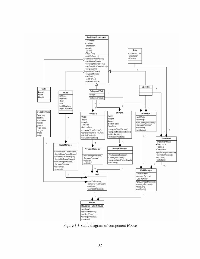
Figure 3.3 Static diagram of component House
32
3.2 Roof Model
The roof cover is made up of many shingles, most of which have rectangular shape. The
roof sheath is made up of plywood sheets, most of which have rectangular shape, too. A masonry
wall is made up of bricks. We define a 2D plane on which shingles , plywood or bricks lie. For
example, a gable-roof house has two planes for shingle and plywood and a hip-roof house has
four planes for shingles and plywood. A rectangular house with four walls has four planes for
bricks. Hereafter, we refer a single piece of shingle, plywood or brick as a tile.
Each tile is assigned a detachment time, the time a tile will be detached from the plane.
This value could also be assigned according to the data obtained from a wind tunnel test.
1) Information for each shingle
TILE_SHAPE_TYPE shape;
float top1,bot1,top2,bot2;
float texCoordX, texCoordY;
float thickness;
double position[3];
float detachTime;
long countOfForce;
2) Information for shingles on one roof plane
• TILE_DIRECTION: This flag identifies the 2D plane, currently supports
maximum four 2D planes . It could easily be modified to support more 2D planes
for buildings with complex shapes.
• A rectangular bounding box used for each shingle with width, length and height.
33
• Overlap-Width, overlap-Length is width, length for overlapping among shingles
respectively.
• Roof plane orientation.
• m_row number of rows of shingle on the roof plane.
• m_col number of columns of shingle on the roof plane.
• m_number total number of shingles
• m_numberOfRow: indices of the position to start lay shingle
• m_startColumn: indices of the position to start lay shingle
• TILE_ARRAY_TYPE array;
• getWindForce(vsVector &windSpeed, vsVector &shingleSpeed, float angle);
• calculateShinglNumber(double top,double bot, double height);
• cut(TileInformation *s, Rect2D &rect, LineSegment2D &line);
• Generate shingles on a hip roof
• clippingCode(double x, double y, double xcl1, double ycl1, double xcl2, double
ycl2);
• intersect(double x0, double y0,double x1,double y1, double xclipl, double yclipb,
double xclipr, double yclipt);
• isLeftCut(TILE_SHAPE_TYPE shape);
We assume that the house size along Y axis (Ysize) Y axis of a house is assumed to
always be greater or equal to the house size along the X axis (Xsize). Hence for the hip roof,
trapezoidal-shaped roof planes only appear along the Y axis. Roof planes along the X axis
always have a triangular shape. The normal shape of a shingle or a sheet of plywood is
34
rectangular. To properly fit the gable roof, all shingles and plywood are rectangular. But for hip
roof, shingles, and plywood with triangular, trapezoidal or pentagon shapes are needed near the
ridge of the roof plane. We take triangle and rectangle shapes as special case of trapezoids. Now
the shingles and plywood automating generation problem is as follows: Given a trapezoid, how
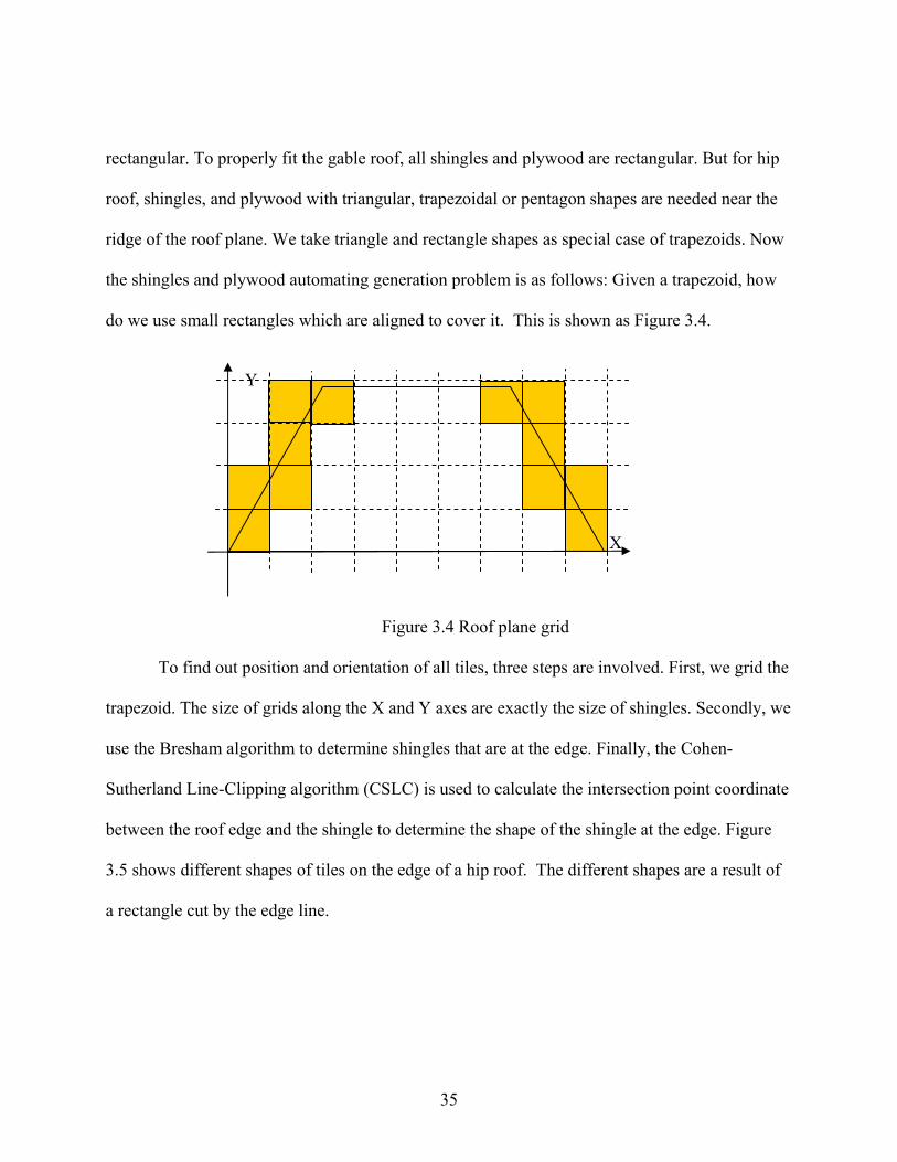
do we use small rectangles which are aligned to cover it. This is shown as Figure 3.4.
X
Y
Figure 3.4 Roof plane grid
To find out position and orientation of all tiles, three steps are involved. First, we grid the
trapezoid. The size of grids along the X and Y axes are exactly the size of shingles. Secondly, we
use the Bresham algorithm to determine shingles that are at the edge. Finally, the Cohen-
Sutherland Line-Clipping algorithm (CSLC) is used to calculate the intersection point coordinate
between the roof edge and the shingle to determine the shape of the shingle at the edge. Figure
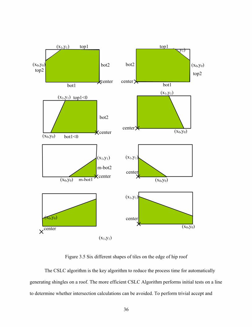
3.5 shows different shapes of tiles on the edge of a hip roof. The different shapes are a result of
a rectangle cut by the edge line.
35
(x0,y0)
top2
(x1,y1)
(x0,y0)
bot2
center bot1<0
top1<0
(x0,y0)
(x1,y1)
center (x0,y0)
(x1,y1)
m-bot2
m-bot1(x0,y0)
(x1,y1)
center
(x1,y1)
(x0,y0)
(x1,y1)
center
(x0,y0)
(x1,y1)
center (x0,y0)
center
bot2top2
bot1
top1
center
(x1,y1)
bot2
bot1
top1
center
Figure 3.5 Six different shapes of tiles on the edge of hip roof
The CSLC algorithm is the key algorithm to reduce the process time for automatically
generating shingles on a roof. The more efficient CSLC Algorithm performs initial tests on a line
to determine whether intersection calculations can be avoided. To perform trivial accept and
36

reject tests, we extend the edges of the clip rectangle to divide the plane of the clip rectangle into
nine regions. Each region is assigned a 4-bit code determined by where the region lies with
respect to the outside half-planes of the clip-rectangle edges. Each bit in the out-code is set to
either 1 or 0. The 4 bits in the code correspond to Table 3.1.
Table 3.1 Out-code definition in CSLC algorithm
Bit 1 outside half-plane of top edge, above top edge
Bit 2 outside half-plane of bottom edge, below bottom edge
Bit 3 outside half-plane of right edge, to the right of right edge
Bit 4 outside half-plane of left edge, to the left of left edge
Steps for Cohen-Sutherland algorithm is as following:
1) End-points pairs are check for trivial acceptance or trivial rejected using the out-
code.
2) If not trivial-acceptance or trivial-rejected, a clip edge is divide into two
segments.
3) Iteratively clipping by testing trivial-acceptance or trivial-rejected, and divided
into two segments until completely inside or trivial-rejected.
In summary, the C-S algorithm is efficient when out-code testing can be done cheaply
(for example, by doing bitwise operations in assembly language) and trivial acceptance or
rejection is applicable to the majority of line segments. (For example, with large windows -
everything is inside , or with small windows - everything is outside).
37
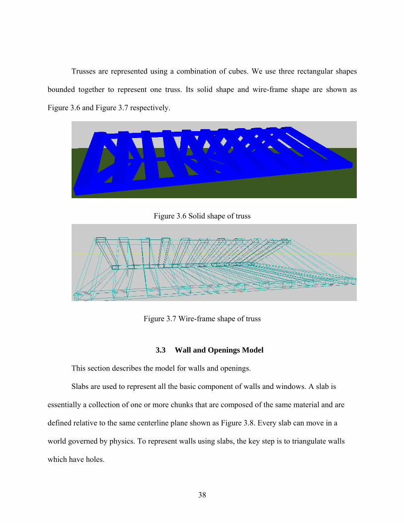
Trusses are represented using a combination of cubes. We use three rectangular shapes
bounded together to represent one truss. Its solid shape and wire-frame shape are shown as
Figure 3.6 and Figure 3.7 respectively.
Figure 3.6 Solid shape of truss
Figure 3.7 Wire-frame shape of truss
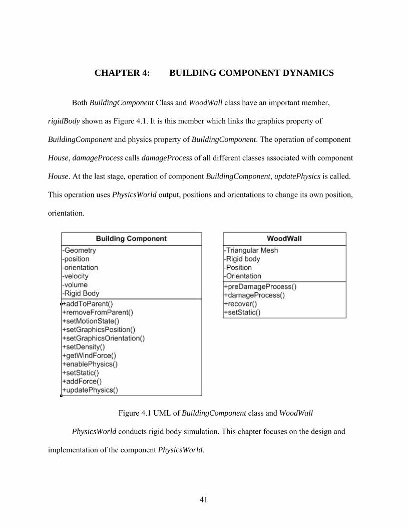
3.3 Wall and Openings Model
This section describes the model for walls and openings.
Slabs are used to represent all the basic component of walls and windows. A slab is
essentially a collection of one or more chunks that are composed of the same material and are
defined relative to the same centerline plane shown as Figure 3.8. Every slab can move in a
world governed by physics. To represent walls using slabs, the key step is to triangulate walls
which have holes.
38
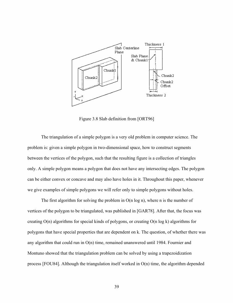
Figure 3.8 Slab definition from [ORT96]
The triangulation of a simple polygon is a very old problem in computer science. The
problem is: given a simple polygon in two-dimensional space, how to construct segments
between the vertices of the polygon, such that the resulting figure is a collection of triangles
only. A simple polygon means a polygon that does not have any intersecting edges. The polygon
can be either convex or concave and may also have holes in it. Throughout this paper, whenever
we give examples of simple polygons we will refer only to simple polygons without holes.
The first algorithm for solving the problem in O(n log n), where n is the number of
vertices of the polygon to be triangulated, was published in [GAR78]. After that, the focus was
creating O(n) algorithms for special kinds of polygons, or creating O(n log k) algorithms for
polygons that have special properties that are dependent on k. The question, of whether there was
any algorithm that could run in O(n) time, remained unanswered until 1984. Fournier and
Montuno showed that the triangulation problem can be solved by using a trapezoidization
process [FOU84]. Although the triangulation itself worked in O(n) time, the algorithm depended
39

on the trapezoidization method, which was a O(n log n) algorithm, thus making the whole
algorithm run in O(n log n) time. Tarjan and van Wyk in 1986 published another algorithm
which has the advantage that it could be adapted to solve other problems in linear time [TAR86].
In 1991, Chazelle announced a deterministic algorithm that runs in O(n log* n). Although it
produced a good result, it was very complicated to implement. In 2000, Amato, Goodrich, and
Ramos finally discovered a randomized algorithm that runs in O(n log* n) time, but which did
not use complicated data structures [AMA00], and thus was considered better and easier to
implement. The current research uses the trapezoidization method by Fournier and Montuno.
40
CHAPTER 4: BUILDING COMPONENT DYNAMICS
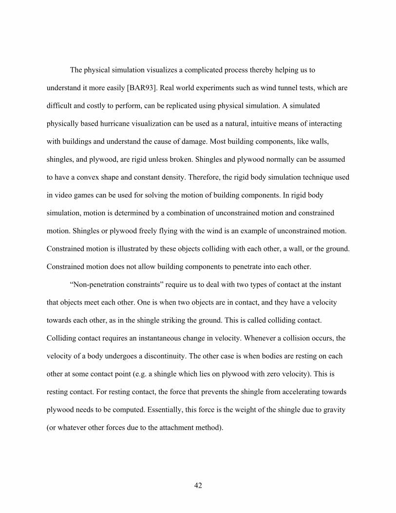
Both BuildingComponent Class and WoodWall class have an important member,
rigidBody shown as Figure 4.1. It is this member which links the graphics property of
BuildingComponent and physics property of BuildingComponent. The operation of component
House, damageProcess calls damageProcess of all different classes associated with component
House. At the last stage, operation of component BuildingComponent, updatePhysics is called.
This operation uses PhysicsWorld output, positions and orientations to change its own position,
orientation.
Figure 4.1 UML of BuildingComponent class and WoodWall
PhysicsWorld conducts rigid body simulation. This chapter focuses on the design and
implementation of the component PhysicsWorld.
41
The physical simulation visualizes a complicated process thereby helping us to
understand it more easily [BAR93]. Real world experiments such as wind tunnel tests, which are
difficult and costly to perform, can be replicated using physical simulation. A simulated
physically based hurricane visualization can be used as a natural, intuitive means of interacting
with buildings and understand the cause of damage. Most building components, like walls,
shingles, and plywood, are rigid unless broken. Shingles and plywood normally can be assumed
to have a convex shape and constant density. Therefore, the rigid body simulation technique used
in video games can be used for solving the motion of building components. In rigid body
simulation, motion is determined by a combination of unconstrained motion and constrained
motion. Shingles or plywood freely flying with the wind is an example of unconstrained motion.
Constrained motion is illustrated by these objects colliding with each other, a wall, or the ground.
Constrained motion does not allow building components to penetrate into each other.
“Non-penetration constraints” require us to deal with two types of contact at the instant
that objects meet each other. One is when two objects are in contact, and they have a velocity
towards each other, as in the shingle striking the ground. This is called colliding contact.
Colliding contact requires an instantaneous change in velocity. Whenever a collision occurs, the
velocity of a body undergoes a discontinuity. The other case is when bodies are resting on each
other at some contact point (e.g. a shingle which lies on plywood with zero velocity). This is
resting contact. For resting contact, the force that prevents the shingle from accelerating towards
plywood needs to be computed. Essentially, this force is the weight of the shingle due to gravity
(or whatever other forces due to the attachment method).
42
Constrained motion has been the object of many studies. Moore and Wilhelms [MOR88]
provide one of the earliest treatments of two fundamental problems in dynamics simulation:
collision detection and collision response. Collision detection determines over a given time
interval whether any points of the two objects occupy the same location in space simultaneously
[HAD04]. Collision response determines the objects’ velocity and acceleration after a collision is
detected.
The rest of this chapter is organized as following. First, unconstrained motion
representation of rigid body i.e. ODE, is established. Second, collision detection methods used in
the current research are described. Finally, these collision responses are discussed.
4.1 Equation of Unconstrained Motion
Given an object shown as Figure 4.2, its mass of center lies at x(t), applying force F(t) at
point r(t) on this object, equation of unconstrained motion will give us the linear velocity,
angular velocity, position and orientation of this object. Then linear velocity v(t) is defined as:
)()( txtv•
= (4.1)
Linear momentum P(t) is given by:
)()( tMvtP = (4.2)
43
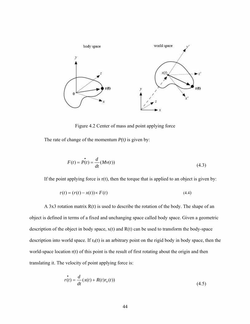
Figure 4.2 Center of mass and point applying force
The rate of change of the momentum P(t) is given by:
))(()()( tMvdtdtPtF ==
•
(4.3)
If the point applying force is r(t), then the torque that is applied to an object is given by:
)())()(()( tFtxtrt ×−=τ (4.4)
A 3x3 rotation matrix R(t) is used to describe the rotation of the body. The shape of an
object is defined in terms of a fixed and unchanging space called body space. Given a geometric
description of the object in body space, x(t) and R(t) can be used to transform the body-space
description into world space. If r0(t) is an arbitrary point on the rigid body in body space, then the
world-space location r(t) of this point is the result of first rotating about the origin and then
translating it. The velocity of point applying force is:
))()()(()( 0 trtRtxdtdtr +=
•
(4.5)
44
We build the body space by specifying the center of mass of the body, which lies at the
origin; the world-space location of the center of mass is always given directly by x(t). We write
out the components of R(t) as:
⎟⎟⎟
⎠
⎞
⎜⎜⎜
⎝
⎛
=
zzyzxz
zyyyxy
zxyxxx
rrrrrrrrr
tR )(
Spinning of a rigid body is described as a vector ω(t). The direction of ω(t) gives the
direction of the axis about which the body is spinning. The magnitude of ω(t) tells how fast the
body is spinning. ω(t) and R(t) can be connected using:
⎟⎟⎟⎟
⎠
⎞
⎜⎜⎜⎜
⎝
⎛
⎟⎟⎟
⎠
⎞
⎜⎜⎜
⎝
⎛×
⎟⎟⎟
⎠
⎞
⎜⎜⎜
⎝
⎛
×⎟⎟⎟
⎠
⎞
⎜⎜⎜
⎝
⎛×=
•
zz
zy
zx
yz
yy
yx
xz
xy
xx
rrr
trrr
trrr
ttR )()()()( ωωω , where × means cross product.
From equation (4.5), we have
)()()()( trttxtr ×+=••
ω (4.6)
To simplify , we define ω* as matrix •
)(tR
⎟⎟⎟
⎠
⎞
⎜⎜⎜
⎝
⎛
−−
−
00
0
xy
xz
yz
ωωωωωω
where xω , yω , and zω are component of ω(t). Then we have
)()()( * tRttR ω=•
The shape and mass distribution of the body is described by inertia tensor J(t). J(t) is a
3x3 matrix. It can be thought of as a scaling factor between angular momentum and angular
45
velocity. This matrix is computed in body space and then transformed as needed to world space.
Inertia in body space is pre-computed. The conversion of inertia from body space to world space
is:
Tbody tRItRtI )()()( = (4.7)
Where,
⎟⎟⎟
⎠
⎞
⎜⎜⎜
⎝
⎛
−−−−−
=
zzyzxz
yzyyxy
xzxyxx
body
IIIIIIIII
I_
(4.8)
Assume the object occupy a volume, then
∫ +=volumexx dmzyI )( 22 (4.9)
∫ +=volumeyy dmzxI )( 22 (4.10)
∫ +=volumezz dmyxI )( 22 (4.11)
∫= volumexy dmxyI )( (4.12)
∫= volumexz dmxzI )( (4.13)
∫= volumeyz dmyzI )( (4.14)
Angular momentum L(t) is computed by
)()()( ttItL ω=
The rate of change of the angular momentum is given by
46
)()())(()(
)())(())(()(
)())()(())(()(
)()())(()(
)())(())(()())()(()()(
**
**
tRRIRRItdtdtI
tRRIRRItdtdtI
tRdtdRIRIR
dtdt
dtdtI
tRRIdtdt
dtdtI
ttIdtdt
dtdtIttI
dtdtLt
TTbody
Tbody
Tbody
Tbody
Tbody
Tbody
Tbody
ωωωωω
ωωωω
ωω
ωω
ωωωτ
++=
++=
++=
+=
+===•
Since 0)()( * =tT ωω
Hence we got the Euler equation:
ωωωτ Tbody RRIt
dtdtIt *))(()()( +=
The system state Y(t) that each body has associated with it is described as:
⎟⎟⎟⎟⎟
⎠
⎞
⎜⎜⎜⎜⎜
⎝
⎛
=
)()()()(
)(
tLtPtRtx
tY
From this state, other important quantities may be computed.
MtPtV )()( =
)()()( 1 tLtIt −=ω
The derivatives of each component of the state are given by:
⎟⎟⎟⎟⎟
⎠
⎞
⎜⎜⎜⎜⎜
⎝
⎛
=
⎟⎟⎟⎟⎟
⎠
⎞
⎜⎜⎜⎜⎜
⎝
⎛
=
)()(
)(*)()(
)()()()(
)(
ttF
tRttV
tLtPtRtx
dtdtY
dtd
τ
ω
47
This is the differential equation to be solved to compute the trajectories and orientations of the
bodies at various points in time.
4.2 Collision Detection
A distinct area of research concerns itself with the problem of detecting the intersection
or the computing separation of two bodies. GJK [GIL90] and Lin-Canny algorithms [LIN91]
both handle convex polyhedral collision detection very well. Other algorithms are variations on
these basic two algorithms. Quinlan (1994) uses a collision detector that can return contacts for all
collision situations between vertices, edges and faces [QUI94]. Schmidl (2004) uses a method of
fast update of OBB trees for simulations with thousands of contacts [SCH04].
Collision detection is usually divided into two phases. The task of the broad phase is to
quickly determine which bodies may be in contact and which bodies cannot collide. The narrow
phase then goes through the list of possibly colliding objects and determines the detailed contact
information. Bergen [Berg04] gives a good collision detection overview. Two very efficient
algorithms for the narrow phase are Mirtich's Voronoi Clip (V-Clip) algorithm [Mirt98b] and the
Gilbert-Johnson-Keerthi (GJK) algorithm1 [GiJK88]. Both are explained in detail in Coutinho
[Cout01]. Many algorithms for the narrow phase only return information about the pair of closest
points of two bodies. This is not enough for the simulation as a whole contact set is needed,
which often involves more than one contact. Mirtich [Mirt98c] shows how the V-Clip algorithm
can be used to model contact regions. Redon [Redo04] gives an overview on recent works on
continuous collision detection methods that guarantee consistent simulations by computing the
time of first contact.
48
Collision detection methods are categorized into two types: discrete methods and
continuous methods. Discrete collision detection methods sample the objects’ trajectories at
discrete times and report inter-penetrations only. This method must use backtracking methods to
compute the time of the first contact. Backtracking methods attempt to compute the first time of
contact by recursively subdividing the time interval after an inter-penetration has been detected.
Assume that the current time interval is [t0, t0+∆t], and assume an inter-penetration has been
detected at time tn+1. Essentially, one time of first contact te is estimated in this interval (for
example, by taking the midpoint of the time interval). Then the objects’ positions are computed
at this instant and an inter-penetration detection is performed again. Depending on whether the
objects interpenetrate or not, the algorithm decides that the first time of collision is in [t0, te] or
[te, t0+∆t ], respectively, and loops on this new interval. The process stops when the amount of
interpenetration is smaller than a predetermined threshold. Apparently, the computational cost of
backtracking can be high when objects are complex or when they have interpenetrated much.
Besides, since backtracking is only performed when an inter-penetration has been detected, non-
connected objects, or even non-convex objects, can enter a configuration from which they could
not get out. As a result, they can miss collisions when the objects move rapidly or are small.
Moreover, even when an inter-penetration detected, it is often difficult to reposition the objects
in a contacting position. One reason is that computing the penetration depth for general objects is
difficult because the objects’ motion is not taken into account. Consequently, discrete collision
detection methods cannot guarantee the existence of complete interpenetration-free paths, and
can lead to inconsistent, unrealistic, or even unreachable states.
49
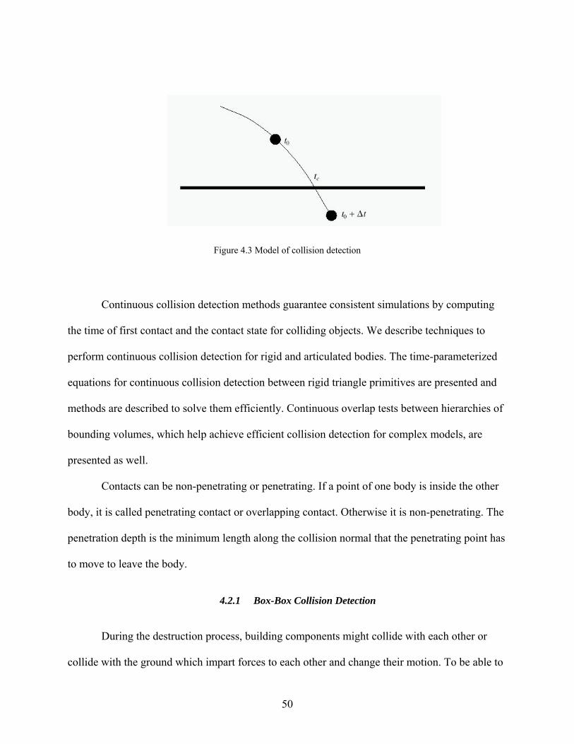
Figure 4.3 Model of collision detection
Continuous collision detection methods guarantee consistent simulations by computing
the time of first contact and the contact state for colliding objects. We describe techniques to
perform continuous collision detection for rigid and articulated bodies. The time-parameterized
equations for continuous collision detection between rigid triangle primitives are presented and
methods are described to solve them efficiently. Continuous overlap tests between hierarchies of
bounding volumes, which help achieve efficient collision detection for complex models, are
presented as well.
Contacts can be non-penetrating or penetrating. If a point of one body is inside the other
body, it is called penetrating contact or overlapping contact. Otherwise it is non-penetrating. The
penetration depth is the minimum length along the collision normal that the penetrating point has
to move to leave the body.
4.2.1 Box-Box Collision Detection
During the destruction process, building components might collide with each other or
collide with the ground which impart forces to each other and change their motion. To be able to
50
handle the forces acting on bodies that collide, collision must first be detected. Over 80 percent
of collisions in the building damage process are box-box collisions. The subsection gives a detail
description about the collisions between boxes and serves as one of the cornerstones for our
performance increase measure in the next subsection.
The statement of the problem is: There are two boxes. One box is located at position pa
with orientation matrix Ra. Its dimension is described using 3D vector ea. We put it this way:
Box A (pa, Ra, ea). Another box is described as Box B (pb, Rb, eb). Now we need to determine
whether they collide or not. If yes, we need to know the number of contact points, each contact
normal, the maximum penetration depth along that normal and the type of contact.
We start with the separating hyperplane theorem, a result of convex analysis. Given two
convex sets A and B, either the two sets are intersecting or there exists a separating hyperplane P
such that A is on one side of P and B is on the other. A separating axis is a line L perpendicular
to P. Two polyhedral objects may come into contact in three different ways with respect to their
features: face-face, face-edge, and edge-edge if we consider a vertex as part of an edge. For the
face-face and face-edge cases, the face normal is used to project axes separately. For the edge-
edge case, the separating axis is the cross product of these two edges. In summary, to test the
separability of two polyhedral objects, the following separating axes test should be performed:
1) Axes parallel to each face normal of object A
2) Axes parallel to each face normal of object B
3) Axes parallel to the vectors resulting from the cross products of all edges in A
with all edges in B
51
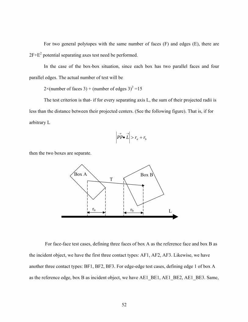
For two general polytopes with the same number of faces (F) and edges (E), there are
2F+E2 potential separating axes test need be performed.
In the case of the box-box situation, since each box has two parallel faces and four
parallel edges. The actual number of test will be
2×(number of faces 3) + (number of edges 3)2 =15
The test criterion is that- if for every separating axis L, the sum of their projected radii is
less than the distance between their projected centers. (See the following figure). That is, if for
arbitrary L
ba rrLPP +>•→→
then the two boxes are separate.
ra rb L
T Box B Box A
For face-face test cases, defining three faces of box A as the reference face and box B as
the incident object, we have the first three contact types: AF1, AF2, AF3. Likewise, we have
another three contact types: BF1, BF2, BF3. For edge-edge test cases, defining edge 1 of box A
as the reference edge, box B as incident object, we have AE1_BE1, AE1_BE2, AE1_BE3. Same,
52
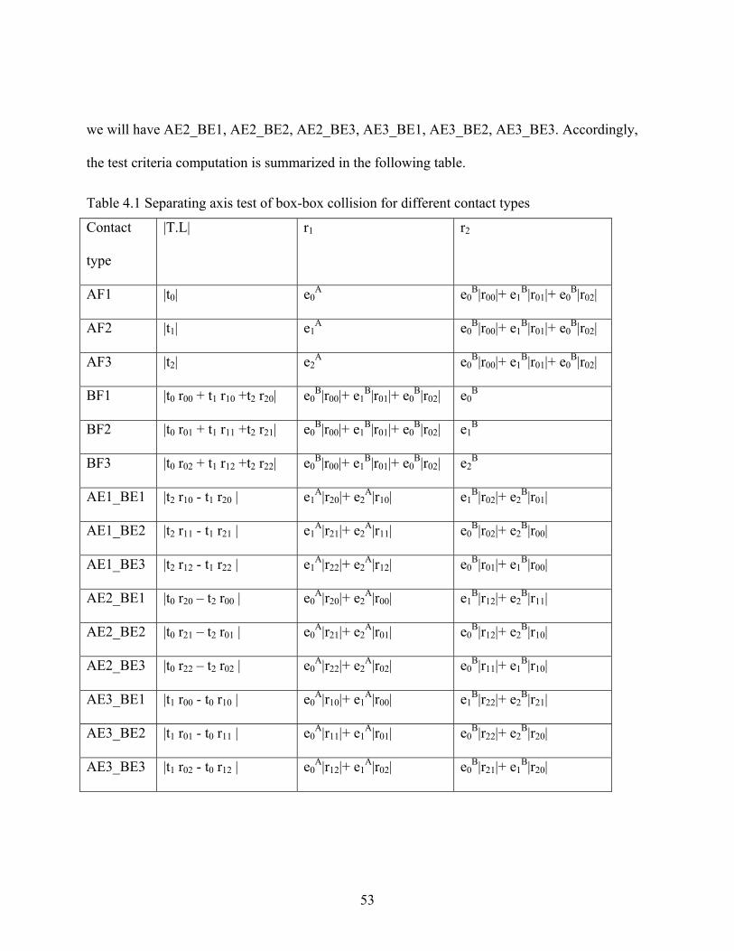
we will have AE2_BE1, AE2_BE2, AE2_BE3, AE3_BE1, AE3_BE2, AE3_BE3. Accordingly,
the test criteria computation is summarized in the following table.
Table 4.1 Separating axis test of box-box collision for different contact types
Contact
type
|T.L| r1 r2
AF1 |t0| e0A e0
B|r00|+ e1B|r01|+ e0
B|r02|
AF2 |t1| e1A e0
B|r00|+ e1B|r01|+ e0
B|r02|
AF3 |t2| e2A e0
B|r00|+ e1B|r01|+ e0
B|r02|
BF1 |t0 r00 + t1 r10 +t2 r20| e0B|r00|+ e1
B|r01|+ e0B|r02| e0
B
BF2 |t0 r01 + t1 r11 +t2 r21| e0B|r00|+ e1
B|r01|+ e0B|r02| e1
B
BF3 |t0 r02 + t1 r12 +t2 r22| e0B|r00|+ e1
B|r01|+ e0B|r02| e2
B
AE1_BE1 |t2 r10 - t1 r20 | e1A|r20|+ e2
A|r10| e1B|r02|+ e2
B|r01|
AE1_BE2 |t2 r11 - t1 r21 | e1A|r21|+ e2
A|r11| e0B|r02|+ e2
B|r00|
AE1_BE3 |t2 r12 - t1 r22 | e1A|r22|+ e2
A|r12| e0B|r01|+ e1
B|r00|
AE2_BE1 |t0 r20 – t2 r00 | e0A|r20|+ e2
A|r00| e1B|r12|+ e2
B|r11|
AE2_BE2 |t0 r21 – t2 r01 | e0A|r21|+ e2
A|r01| e0B|r12|+ e2
B|r10|
AE2_BE3 |t0 r22 – t2 r02 | e0A|r22|+ e2
A|r02| e0B|r11|+ e1
B|r10|
AE3_BE1 |t1 r00 - t0 r10 | e0A|r10|+ e1
A|r00| e1B|r22|+ e2
B|r21|
AE3_BE2 |t1 r01 - t0 r11 | e0A|r11|+ e1
A|r01| e0B|r22|+ e2
B|r20|
AE3_BE3 |t1 r02 - t0 r12 | e0A|r12|+ e1
A|r02| e0B|r21|+ e1
B|r20|
53
In the above table, e0A, e1
A and e2A is the half length of box A’s three sides respectively
and e0B, e1
B and e2B is the half length of the box B’s three sides respectively. Vector T=(t0, t1, t2)
is the center position of Box B relative to Box A. Matrix R is the relative rotation between Ra
and Rb
If there the test criterion is met, then a collision occurs and the response computation
requires the following contact point information:
1) Contact type which tells the reference to the two colliding bodes
2) Position
3) Normal vector, which is normal to the touching surfaces
4) Penetration depth
4.2.2 GJK Collision Detection
Box-box collision is the most common collision type in the current research. However,
shingles and plywood at the ridge of hip-roof could have triangal, trapezoidal or pentagon
shapes, as shown in Figure 3.4. The GJK algorithm computes the distance between a pair of
convex objects. The distance between objects A and B, denoted by d(A,B), is defined by:
},||:min{||),( ByAxyxBAd ∈∈−=
The algorithm can be tailored to return a pair of closest points, which is a pair of points:
point a is in object A and point b is in object B for which ),(|||| BAdba =− .
We express the distance between A and B in terms of their Minkowski sum A − B as:
||(||),( BAvBAd −=
where v(C) is defined as the point in C nearest to the origin, i.e.,
54
CCv ∈)( and }||:min{||||)(|| CxxCv ∈=
Clearly, for a pair of closest points, we have a-b=v(A-B).
GJK is essentially a descent method for approximating v(A − B) for convex objects A
and B. In each iteration a simplex is constructed that is contained in A − B and lies nearer to the
origin than the simplex constructed in the previous iteration.
The basic step of GJK algorithm is as following:
1) Arbitrarily construct a simplex inside the object.
2) Find the point V of this simplex closest to the origin.
3) Compute support point w for the vector –V.
4) Add support point w to the current simplex to get a simplex.
5) Compute the new point Vnew closest to the origin of the new simplex.
6) Discard all vertices that do not contribute to Vnew to get another simplex
7) Loop to the second step.
4.3 Collision Response computation
Approaches suggested to compute collision response include penalty methods, impulse-
based methods and constraint based methods.
Penalty methods are generally used when no precise contact information is available, as
they compute the contact forces from the amount of interpenetration between contacting objects
[WIT87], [KAC03]. This correction force tries to push the point back to the valid position. An
energy function is defined using constraints. The energy is zero if constraints are met. Otherwise,
the energy grows. The penalty force minimizes energy and it acts in the direction of the
55
maximum descent of energy. The penalty force is acting like a spring force with a spring
constant of K. Colliding contact and resting contact can both be approximated by
(hypothetically) inserting a spring between the contact points of each body. For the resting
contact, springs are removed if the bodies are separating, so bodies keep their contact. For the
colliding contact, one spring with constant Kapproach is used if bodies are approaching while
another spring with constant Kseparate is used if bodies are separating. The advantage of the
penalty methods is its simplicity. It automatically corrects deviations from valid positions and
thus can be used for error correction. However, an appropriate spring constant has to be chosen.
This constant depends on the properties of the current object in the scene (for example
coefficient of restitution and mass). However, the simulated scenario requires a large stiffness
value, and so the differential equations become “stiff” making them increasingly more difficult
to solve. Consequently, accuracy can be hard to achieve in real time.
Impulse-based methods model all the forces between bodies through a series of impulses.
For example in Figure 4, the ball receives a series of impulses as it bounces and collides with the
floor after falling off the slope. Even when the ball has stopped bouncing and is rolling we still
model the forces between the ball and floor as impulses. Imagine a block resting on the ground.
Instead of there being a constant force being applied upwards counteracting gravity and keeping
it at rest, in the impulse model the block receives a rapid series of impulses being applied at each
of its corners. It is these impulses that keep it from accelerating downwards. However they will
also cause the block to vibrate rapidly but the values can be chosen such that the amplitude of the
vibration is less than a pixel, hence it appears stationary to the user. Although this seems like a
departure from what happens in reality, it is in most cases an acceptable tradeoff for
56
computational speed. So in some sense, the impulse method preserves important physical
quantities, such as the average velocity of the object and the average forces on the object. All
contacts are modeled as collisions. Between collisions, the bodies move along ballistic
trajectories. If friction and restitution are incorporated into the collision model, then the resulting
impulse trains can generate persistent phenomena such as rolling, sliding, and settling [Sch04].
Assuming that the relative velocity is already negative, impulse J need to be computed which
will instantaneously change the velocities of the two bodies.
The impulse acts in the contact normal direction, i.e., . The empirical law for
frictionless collisions states that:
)( 0tnjJ∧
=
−+ −= relrel vv ε (4.15)
Here ε is the coefficient of restitution. It can range from 0 to 1. A value of 0 means that all the
energy is lost and there is no bounce. A value of 1 means that all the energy is kept in the system
and the bodies will act perfectly bouncy.
Constraint based methods take into account all contact points at a given instant in time in
order to compute the forces required at all contacts [HAR03]. Its basic idea is to convert each
constraint into a force imposed on its related objects. The principle of virtual work [WIT90] is
used; this stipulates that constraint forces do not add or remove energy. Hence, it is used to
compute constraints forces. This principle also implies that the constraint force is opposed to the
direction in which the system is forbidden to move. The rapid progress made in this method
gives the rigid body simulation a fast, stable and realistic solution. Current research focuses on
this method.
57
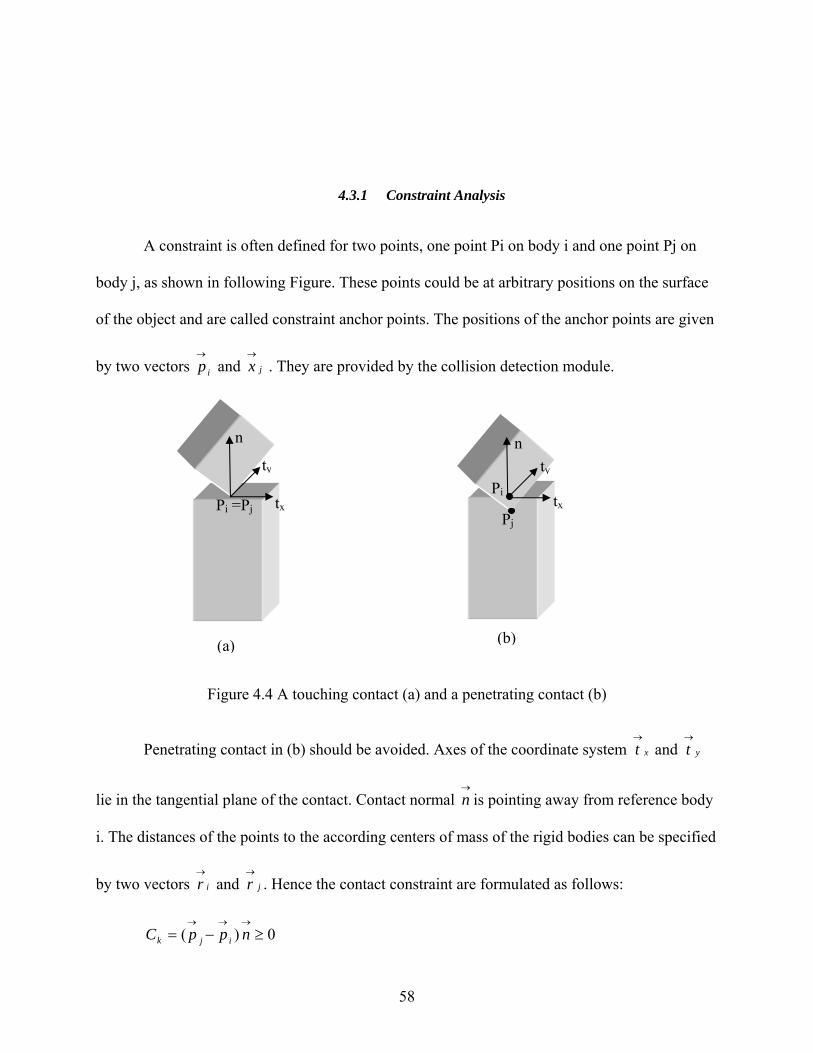
4.3.1 Constraint Analysis
A constraint is often defined for two points, one point Pi on body i and one point Pj on
body j, as shown in following Figure. These points could be at arbitrary positions on the surface
of the object and are called constraint anchor points. The positions of the anchor points are given
by two vectors and . They are provided by the collision detection module. ip→
jx→
n
tx
ty
nty
txPi
PjPi =Pj
(a) (b)
Figure 4.4 A touching contact (a) and a penetrating contact (b)
Penetrating contact in (b) should be avoided. Axes of the coordinate system and
lie in the tangential plane of the contact. Contact normal is pointing away from reference body
i. The distances of the points to the according centers of mass of the rigid bodies can be specified
by two vectors and . Hence the contact constraint are formulated as follows:
xt→
yt→
→
n
ir→
jr→
0)( ≥−=→→→
nppC ijk
58
kC describes the separation distance in the direction of . Hence relative contact
velocity in the direction of is , and
→
n
→
n•
kC
))(()(•→→→
•→
•→→•
−+−= nppppnC ijijk
))(()(2)(••→→→
•→
•→
•→
•→
•→→••
−+−+−= nppppnppnC ijijijk
))((•→→→
− npp ij and are much smaller than the other term on the right side
since the penetration at the contact is small, therefore:
))((••→→→
− npp ij
)(•→
•→→•
−= ijk ppnC (4.16)
)(2)(•→
•→
•→
••→
••→→••
−+−= ijijk ppnppnC (4.17)
Having found a contact k, and are examined to classify the contact: kC•
kC
If <0, then it is a penetrating contact. If =0, then it is a touching contact without
penetration. If >0, then it is not a contact and will not be reported by the collision detection. If
<0, then the bodies are moving towards each other. This is called colliding contact. If =0,
then the bodies are touching and neither separating nor colliding. This is called resting contact. If
>0, then the bodies are separating. This is called separating contact. In practice, a threshold
limit is used instead of 0. For example resting contact are contacts with
and separating contact are contacts with .
kC kC
kC
•
kC•
kC
•
kC
imitthresholdLCk <•
|| imitthresholdLCk >•
59
Considering equality constraints: If in one time step =0, then the constraint is satisfied
at the moment. If =0, then the constraint will be satisfied in the next time step. But if ≠0,
the deviation will grow and the constraint will be violated in the next time step. If =0 and
=0, the constraint is satisfied and will be satisfied in the next time step. will stay zero as
long as stays zero. With these considerations, different strategies can be formed to deal with
equality constraints:
kC
•
kC•
kC
kC
•
kC•
kC
••
kC
Position-based formulation: If the new position is violating the position constraint ,
we compute a position change of all the bodies, so that the constraints are satisfied again.
kC
Velocity-based formulation: Assume that position constraint is not violated and try to
keep =0. If ≠0 in one time step, then we have to compute a change in the velocities, so
that is corrected to zero.
kC
•
kC•
kC
•
kC
Force-based formulation: Assume that both position constraint and velocity constraint
are met, try to keep acceleration constraint by calculating constraint forces.
kC
•
kC••
kC
For inequality constraints, it is satisfied as long as ≥0. As long as >0, can take
positive and negative values because the deviation is allowed to grow or shrink. Only if ≤0,
has to be zero or positive: ≥0. This means that equality constraints have to be actively
enforced all the time, whereas inequality constraints only have to be enforced if reaches zero.
If is greater than zero, the constraint solver has nothing to do.
kC kC•
kC
kC
•
kC•
kC
kC
kC
60
4.3.2 LCP Formulation
Baraff [BAR89] first used a constraint-based method to calculate forces between rigid
bodies in resting contact. The constraint force magnitudes must meet the following conditions:
1. The constraint forces do not allow bodies to inter-penetrate.
2. The constraint forces can push but not pull.
3. The constraint forces occur only at the contact point; Once two bodies have
separated at a contact point, there is no force at that contact point.
4. Contact forces are continuous as a function of time.
Condition 1 may be written as :
0≥•
kC (4.18)
For resting contact, we always have . Classical mechanics tell us that acceleration
and depend linearly on constraint force, while , , , are independent of
constraint force. If we assume the system has n objects, then condition 1 is rewritten as:
0=•
kC
••→
jp••→
ip→
n•→
n•→
jx•→
ix
0...2211 ≥−+++=••
knknkkk bfafafaC (4.19)
Condition 2 is written as the inequality:
0],,1[ ≥∈∀ ifni
Denote as , as , .
⎥⎥⎥⎥
⎦
⎤
⎢⎢⎢⎢
⎣
⎡
nf
ff
..2
1
→
f
⎥⎥⎥⎥
⎦
⎤
⎢⎢⎢⎢
⎣
⎡
nb
bb
..2
1
→
b
⎥⎥⎥⎥
⎦
⎤
⎢⎢⎢⎢
⎣
⎡
=
nnnn
n
n
aaa
aaaaaa
A
..........
..
..
21
22221
11211
61
Using matrix notation, equation (4.19) is written as:
0≥−=→→••
bfACk , 0≥→
f (4.20)
From condition 3) and condition 4), if , the contact point is vanishing, the constraint
force, f, will be zero. Therefore we have
0>••
kC
01
=∑=
••n
kkk Cf (4.21)
From equation (4.20) and (4.21)
0=−→→→→
bffAfTT
(4.22)
Finding a feasible solution of the two equations above, of is a quadratic programming
problem. In general, this is a NP-hard problem. Baraff used a heuristic method to find an
approximate solution. The heuristic is to find a minimum sum force solution that satisfy
conditions 1) and 2) via solve a linear programming problem. Hopefully the solution for the
constraint force will approximately minimize .
→
f
∑=
••n
kkk Cf
1
Barraf extended this method to colliding contact case, where <0 i.e. bodies are
moving towards each other. The collision impulses can be found by using the collision constraint
equation:
•
kC
0≥+= −+•
kkk vvC ε
Again according to classical mechanics, is a linear function of impulse J. J is zero if
actually exceeds . Hence like resting contact, we have
+kv
+kv −− kvε
62
0)( ≥+ −+kkk Jvv ε and 0≥kJ
An obvious problem of above method is how to solve the quadratic programming
problem in a limited time. Generalized coordinate formulations are proposed as linear-time
solution methods to tackle this problem, such as Featherstone’s Articulated Body Method
(ABM) [FEA87]. To use them, a parameterization of the system in generalized coordinates has
to be found a priori. This depends heavily on the current problem situation. However, there are
no rules about how to find the right parameterization, and generalized coordinates only allow
handling holonomic constraints but not nonholonomic constraints, such as joint limits or
velocity-dependent constraints. To fill this gap, Baraff [BAR96] used Lagrange multipliers to
give formulations with maximal coordinates and achieved the performance comparing to
formulations with formulation generalized coordinates.
For convenience, positions and orientations of object with index i are gathered in one 6-
dimensional vector: . Then, we have: ⎟⎟⎠
⎞⎜⎜⎝
⎛=
)()(
)(tRtx
tsi
ii
⎟⎟⎠
⎞⎜⎜⎝
⎛⎟⎟⎠
⎞⎜⎜⎝
⎛=⎟⎟
⎠
⎞⎜⎜⎝
⎛=⎟⎟
⎠
⎞⎜⎜⎝
⎛==
•
)()(
)(00
)(*)()(
)()(
)()( *3
tRtV
tI
tRttV
tRtx
dtdts
dtdts
i
i
iii
i
i
iii
ωω
Where I3 is 3 by 3 identity matrix. Denote
and , then ⎟⎟⎠
⎞⎜⎜⎝
⎛=
)(00*
3
tI
Hi
i ω ⎟⎟⎠
⎞⎜⎜⎝
⎛=
)()(
)(ttV
tui
ii ω
)()( tuHts iii =•
Now we concatenate , , of all bodies into a single vector respectively: )(tsi )(tui
Tn tstststs ))()...(),(()( 21=
Tn tutututu ))()...(),(()( 21=
63
And denote matrix n by n matrix S as
⎟⎟⎟⎟⎟⎟⎟⎟
⎠
⎞
⎜⎜⎜⎜⎜⎜⎜⎜
⎝
⎛
=
nH
HH
H
S
..0000............0.........0..0000..0000..000
3
2
1
We have:
)()( tHuts =•
(4.23)
Forces and torques are combined into one vector: and we concatenate
all into:
⎟⎟⎠
⎞⎜⎜⎝
⎛=
)()(
)(ttF
tfi
ii τ
)(tf iT
n tftftftF ))()...(),(()( 21=
The mass property matrix of object with index i is also gathered in one 6 by 6 matrix as:
⎟⎟⎠
⎞⎜⎜⎝
⎛=
⎟⎟⎟⎟⎟⎟⎟⎟
⎠
⎞
⎜⎜⎜⎜⎜⎜⎜⎜
⎝
⎛
−−−−−−
=i
i
zzyzxz
yzyyxy
xzxyxxi I
m
IIIIIIIII
mm
m
M0
0
000000000
000000000000000
The global mass matrix
⎟⎟⎟⎟⎟⎟⎟⎟
⎠
⎞
⎜⎜⎜⎜⎜⎜⎜⎜
⎝
⎛
=
nM
MM
M
M
..0000............0.........0..0000..0000..000
3
2
1
(4.24)
The inverse of the global mass matrix
64
⎟⎟⎟⎟⎟⎟⎟⎟
⎠
⎞
⎜⎜⎜⎜⎜⎜⎜⎜
⎝
⎛
=
−
−
−
−
−
1
12
12
11
11
..0000............0..0000..0000..0000..000
nI
Im
Im
W (4.25)
According to Newton’s law, we have )()( tWFtu =•
Using the Euler method to make it discrete, we have:
ttWFtuttu Δ+=Δ+ )()()( (4.26)
A constraint Ck is a function of positions: ))(()( tsCtC kk = . Hence
••
∂∂
== )()))((()( tss
CtsC
dtdtC k
kk
From equation (4.23),
)()( tHus
CtC k
k ∂∂
=•
Define
Hs
CJ k
∂∂
=
J is called the contact Jacobian. It is a 1 by 6n matrix. We have:
)(...)()()()( 2211 tuJtuJtuJtJutC nnk +++==•
(4.27)
Since each contact only involves two objects, assume the two indexing numbers are i and
j, then only Ji, Jj are not zero. Hence, we have:
)()()( tuJtuJtC jjiik +=•
(4.28)
From equation (4.27),
65
kk ctuJtuJdtdtuJtJu
dtdtC +=+==
••••
)()()()())(()(
Where )()( tuJdtdck =
Hence according to the non-interpenetration condition which says constraint force can
push but not pull, we always have
0)()( ≥+=•••
ctuJtCk (4.29)
Using Lagrange multiplier method described in [WIT97], [BAR96], the constraint force
iTin
Ti
ci
J
JF λ
⎟⎟⎟
⎠
⎞
⎜⎜⎜
⎝
⎛
= ..1
. Concatenate Fi into vector F and λi into vector λ
λTconstriant JF = .
Now the equation of the system motion is:
extT fJtuM +=
•
λ)(
where fext is the external force. Therefore, we have:
extT WfWJtu +=
•
λ)( (4.30)
From equation (4.30) and equation (4.29)
0)( ≥++=•
cJWfJWJtC extT
k λ (4.31)
Denote:
TJWJA =
cJWfB ext +=
Equation (4.31) turns into:
66
0≥+ BAλ (4.32)
In series of equations shown above, λ=[ λ1, λ2,… λn] and λ1, λ2,… λn could have unlimited
combinations to satisfy constraints listed above. However, according to section 4.3.2, which says
constraint force can only push, not pull, we have:
nii ≤<∀≥ 0,0λ (4.33)
Combing equation (4.32) and equation (4.33) is a Linear Complementarity Problem
(LCP). Because the above formulation directly uses force constraint, it is called the force-based
formulation method. One of the difficulties with this formulation method is that there is no
guarantee of the existence of a solution, in the presence of contact with Coulomb friction.
Anitescu and Potra [AP97] proposed a velocity-based formulation that guaranteed solvability
regardless of the configuration or number of contacts. Comparing to force-based LCP
formulations, Velocity-based LCP formulations can also easily combine collisions and resting
contacts. We use the analysis contained in section 4.3.1: For inequality constraints, it is satisfied
as long as ≥0. As long as >0, can take positive and negative values because the
deviation is allowed to grow or shrink. Only if in the case that ≤0 which means penetration,
has to be zero or positive:
kC kC•
kC
kC
•
kC
•
≥ 0kC
From equation (4.27), this turns into:
0)( ≥tJu (4.34)
After time step Δt, we still should have:
0)( ≥Δ+ ttJu (4.35)
67
Apply a Euler integration scheme to equation (4.30), we have:
ttWFtuttu Δ+=Δ+ )()()( (4.36)
Where externalfJtF += λ)( (4.37)
From equation (4.36) and equation (4.37), we have:
0))(( ≥Δ+Δ+ tWftWJtuJ externalλ (4.38)
Again, combining equation (4.38) and equation (4.33), we have a LCP problem to solve.
Practically, because the constraints are not about positions but about velocities, numerical
errors stemming from internal approximations can sneak into the computations of the positions
as the simulation proceeds. Most important of all, due to the time step method we use have to be
fixed time step to maintain a fixed frame-rate ro have the simulation be suitable as instructional
courseware. Using a fixed time step means that we have to allow a small penetration depth to
avoid backtracking during the collision detection phase. From Figure 4.3, we can see that at the
time of collision detection, t+Δt, there is a little penetration depth. We adjust the velocity such
that the error can be smaller in the next simulation step by adding a velocity error correction term
to the right hand side (RHS) of the equation (4.34). Hence, we have:
contactbtJu ≥)( (4.39)
Where
tk
b erpcontact Δ
= , 10 ≤≤ erpk (4.40)
Error correction parameter is a measure of how much error reduction should occur in
the next simulation.
erpk
68
Colliding surfaces between two objects are not always completely hard as if they were
made of steel. Guided by the penalty methods, the current research uses a constraint force mixing
(CFM) value to allow only a little penetration and making the constraint “soft”. The mixed
constraint force allows a little penetration to happen at first and then slowly pushes the two
objects away from each other. CFM is a square diagonal matrix. CFM simply adds to the
diagonal of the original system matrix.
If CFM is set to zero, the constraint will be hard. If CFM is set to a positive value, it is
possible to violate the constraint by “pushing on it” (for example, for contact constraints by
forcing the two contacting objects together). In other words, the constraint will be soft and the
softness will increase as CFM increases.
Using a positive value of CFM has the additional benefit of taking the system away from
any singularity and thus improving the factorizer accuracy. If the system is near-singular,
applying CFM can markedly increase stability.
After applying CFM, from equation (4.39) and equation (4.38), we have
λλ cmfcontactexternal KbtWftWJtuJ −≥Δ+Δ+ ))(( , i.e.
0)(1)1( ≥+−Δ
−Δ
+ externalcmf JWfJubt
Kt
JWJ λ
Now,
Denote:
cmfk Kt
WJJAΔ
+=1
externalJWfJubt
B +−Δ
−= )(1
69
We have:
0≥+ BAλ
Combining equation (4.33), we have our final LCP formulation. In the next section, we
will discuss how to solve it.
4.3.3 SOR method to solve LCP problem
In this section, our goal is to solve following LCP problem to find value of λ :
0≥+ BAλ
nii ≤<∀≥ 0,0λ
Given a large sparse matrix system , we decompose A into a strictly lower matrix
L, a diagonal matrix D and a strictly upper triangular matrix U, i.e.
→→
= bxA
UDLA ++=
Now the solution of the matrix system
→−
→−
→
+−= xULDbDx )(11
Using an iterative method, first write the i’th variable as
ii
jn
ij iji
j jjiii
A
xUxLbx
,
1
1
1
0 ,
→−
+=
−
=
→→
→ ∑∑ −−=
The iterative scheme is
ii
k
jn
ij iji
j
k
jjiik
iA
xUxLbx
,
1
1
1
0 ,1
→−
+=
−
=
→→+→ ∑∑ −−=
70
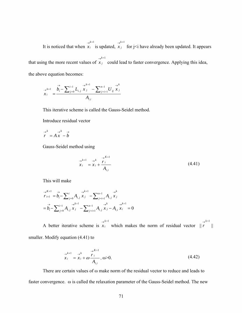
It is noticed that when is updated, for j<i have already been updated. It appears
that using the more recent values of could lead to faster convergence. Applying this idea,
the above equation becomes:
1+→k
ix1+→k
jx
1+→k
jx
ii
k
jn
ij iji
j
k
jjiik
iA
xUxLbx
,
1
1
1
0
1
,1
→−
+=
−
=
+→→+→ ∑∑ −−=
This iterative scheme is called the Gauss-Seidel method.
Introduce residual vector
→→→
−= bxArkk
Gauss-Seidel method using
ii
K
ik
i
k
iA
rxx,
11
+→→+→
+= (4.41)
This will make
01
,1
1 ,1
0
1
,
1
1 ,0
1
,
1
1
=−−−=
−−=+→−
+=
→−
=
+→→
−
+=
→
=
+→→+
+
→
∑∑
∑∑k
iiin
ij
k
jjii
j
k
jjii
n
ij
k
jjii
j
k
jjii
K
i
xAxAxAb
xAxAbr
A better iterative scheme is which makes the norm of residual vector
smaller. Modify equation (4.41) to
1+→ k
ix ||||1+→ k
r
ii
K
ik
i
k
iA
rxx,
11
+→→+→
+= ω , ω>0. (4.42)
There are certain values of ω make norm of the residual vector to reduce and leads to
faster convergence. ω is called the relaxation parameter of the Gauss-Seidel method. The new
71
iterative scheme is called successive over relaxation (SOR). Equation (4.42) can be reformulated
into a more implementation-friendly formula
)()1( 1
1 ,1
0
1
,,
1
∑∑ −
+=
→−
=
+→→→+→
−−+−=n
ij
k
jjii
j
k
jjiiii
K
i
K
i xAxAbA
xx ωω
In rigid body simulation the A-matrix is often symmetric and further the A-matrix is
often positive semi-definite (PSD) or sometimes positive definite (PD). Even if it is PSD, CFM
can be applied to make it PD. To make a long story short, the A-matrix can be made numerically
more pleasant, such that we know a solution exists to the LCP problem.
4.4 Implementation and Conclusion
Experience with several existing physics engines shows that several approaches are
useful to model constraints. There are many details which can interact. This is shown by
applying CFM and error correction parameter in section 4.3.2.
A physical simulation for rigid body is a combination of their components: unconstrained
motion (section 4.1), collision detection (section 4.2) and collision response computation (section
4.3). Timing step methods determine the calling sequence of these components. For the
interactive simulation, fixed time step methods are needed. Fixed time step methods proceed by
making steps of size ∆t and do not subdivide this time step. This implies that collisions are not
handled at the exact collision time. Fixed time step methods are of three types: explicit time step
method, (semi) implicit time step method, and collision-contact-separated time step method.
Explicit time step method proceeds as follows:
1) Collision detection
2) Collision response computation
72

3) Solving ODE to update velocity and position
4) Error correction
5) Increase time step by ∆t
(Semi)implicit time step method tries to detect all contacts that may occur until the time
t+∆t and it proceeds as follows:
1) Position and orientation update by solving ODE and use it to estimate positions
and orientation
2) Collision detection
3) Collision response computation
4) Solving ODE again to get real velocity, position and orientation
5) Error correction
6) Increase time step by ∆t
The collision-contact-separated time step method is presented by Guendelman [GUB03].
The explicit Euler integration method makes the separation of velocity update and position
update easier. Two collision detections are used. After the first collision detection, all contacts
are deemed as colliding contact. After the second collision detection, all contacts detected will
naturally be at resting contact since they are not separating. Hence this method does not need to
distinguish colliding contacts from resting contacts. It proceeds as follows:
1) Collision detection
2) Colliding contact response computation
3) Velocity update
4) Collision detection
73
5) Resting contact solver
6) General constraint solver (i.e. joint)
7) Position update
8) Error correction
9) Increase time step by ∆t
Current research uses a fixed time step method. First of all, axis aligned bounding box
(AABB) information of each object is updated for a broad-phase collision detection.
Unconstrained motion (detailed in section 4.1) of all building components are solved by
advancing the ODE integration one time step. The position, orientation, linear velocity and
angular velocity of each building component are updated. Collision detection detailed in the
previous subsection (4.2.2) is performed to generate contact points and their related information.
Equations (4.8), (4.9)(4.10)(4.11)(4.12)(4.13) and (4.14) are used to pre-compute the inertial of
each object at the object construction phase. Then, given the current object orientation, equation
(4.7) is used to calculate inertial of each object at each frame. Naturally, matrix M in equation
(4.24) and W in equation (4.25) are determined. Given velocity u(t) which including both linear
velocity and angular velocity, Jacobian J.
Time step method in current research includes seven steps:
1) Update AABB of each object
2) Predict unconstrained motion of each object
3) Perform collision detection
4) Compute contact graph
5) Solve contact constraints
74

6) Integrate transforms to update position and velocity of each object
7) Update activation state of each object according to the current frame information
and previous information.
We first show the result of using SOR method to solve LCP formulation for constraint-
based collision response computation. We put an axis-aligned cube with dimension of 2 at a
height level of zero and put the ground at a height level of -9. Ideally, the mass center of the cube
will fall to the height level of -9 and stay there if no bouncing in consideration. We first use
values from Table 4.2.
Table 4.2 Values for test 1
Time step 1/60
Over relaxation coefficient 1.3
Collision detection method Box-box collision
The box-box collision detection method is from section 4.2.1. The value of the Lagrange
multiplier of contact point 1 in each iteration number is shown as Figure 4.5. We can see that at
the fifth iteration, the value converges at about 82. The Lagrange multiplier of contact point
1,2,3,4 is shown as Figure 4.6 and Figure 4.7. Since the collision is detected at time step 0, this
shows that at step 1 the collision force reaches the maximum value and then it varies around the
gravity force of the cube.
75
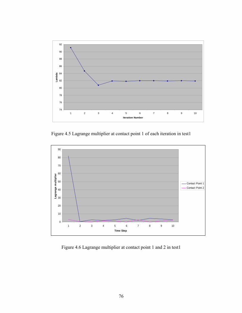
74
76
78
80
82
84
86
88
90
92
1 2 3 4 5 6 7 8 9 10
Iteration Number
Lam
bda
Figure 4.5 Lagrange multiplier at contact point 1 of each iteration in test1
0
10
20
30
40
50
60
70
80
90
1 2 3 4 5 6 7 8 9 10
Time Step
Lagr
ange
mul
tiplie
r
Contact Point 1Contact Point 2
Figure 4.6 Lagrange multiplier at contact point 1 and 2 in test1
76
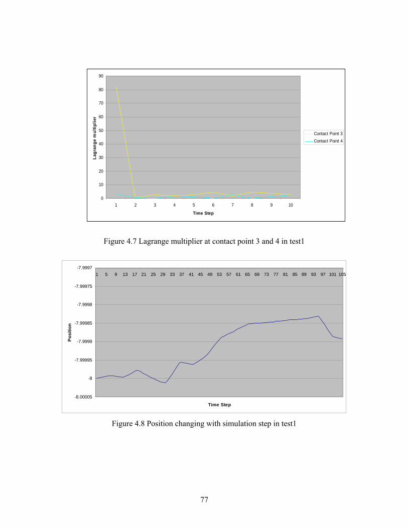
0
10
20
30
40
50
60
70
80
90
1 2 3 4 5 6 7 8 9 10
Time Step
Lagr
ange
mul
tiplie
r
Contact Point 3Contact Point 4
Figure 4.7 Lagrange multiplier at contact point 3 and 4 in test1
-8.00005
-8
-7.99995
-7.9999
-7.99985
-7.9998
-7.99975
-7.99971 5 9 13 17 21 25 29 33 37 41 45 49 53 57 61 65 69 73 77 81 85 89 93 97 101 105
Time Step
Posi
tion
Figure 4.8 Position changing with simulation step in test1
77
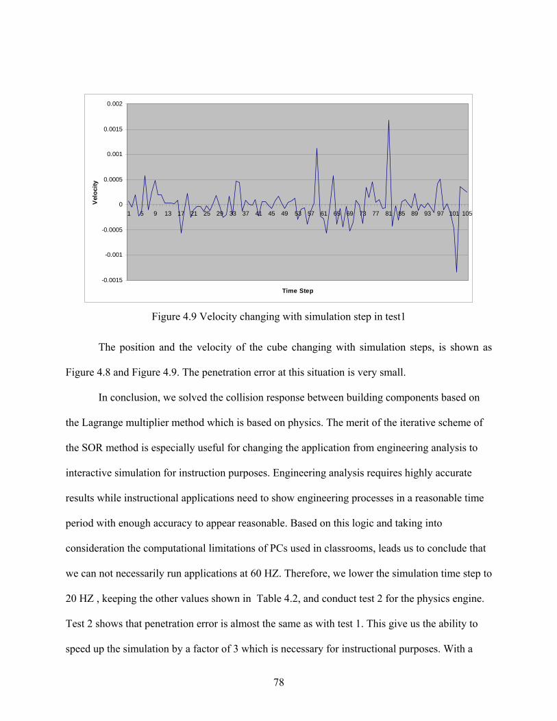
-0.0015
-0.001
-0.0005
0
0.0005
0.001
0.0015
0.002
1 5 9 13 17 21 25 29 33 37 41 45 49 53 57 61 65 69 73 77 81 85 89 93 97 101 105
Time Step
Vel
ocity
Figure 4.9 Velocity changing with simulation step in test1
The position and the velocity of the cube changing with simulation steps, is shown as
Figure 4.8 and Figure 4.9. The penetration error at this situation is very small.
In conclusion, we solved the collision response between building components based on
the Lagrange multiplier method which is based on physics. The merit of the iterative scheme of
the SOR method is especially useful for changing the application from engineering analysis to
interactive simulation for instruction purposes. Engineering analysis requires highly accurate
results while instructional applications need to show engineering processes in a reasonable time
period with enough accuracy to appear reasonable. Based on this logic and taking into
consideration the computational limitations of PCs used in classrooms, leads us to conclude that
we can not necessarily run applications at 60 HZ. Therefore, we lower the simulation time step to
20 HZ , keeping the other values shown in Table 4.2, and conduct test 2 for the physics engine.
Test 2 shows that penetration error is almost the same as with test 1. This give us the ability to
speed up the simulation by a factor of 3 which is necessary for instructional purposes. With a
78
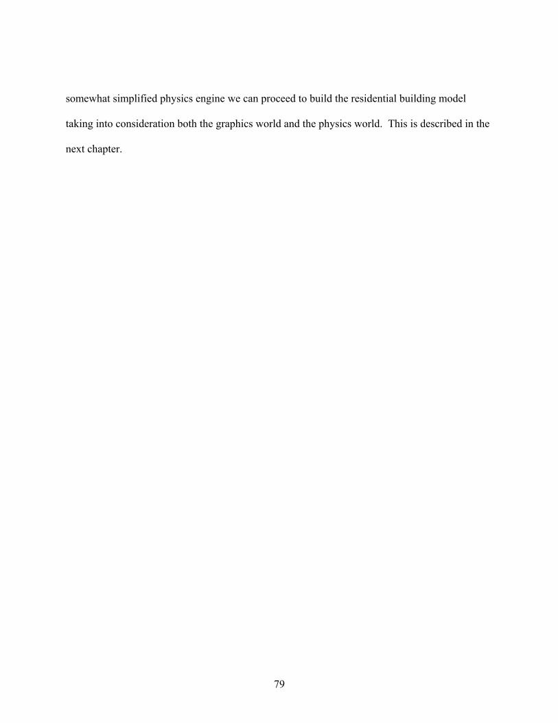
somewhat simplified physics engine we can proceed to build the residential building model
taking into consideration both the graphics world and the physics world. This is described in the
next chapter.
79
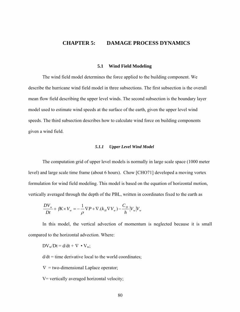
CHAPTER 5: DAMAGE PROCESS DYNAMICS
5.1 Wind Field Modeling
The wind field model determines the force applied to the building component. We
describe the hurricane wind field model in three subsections. The first subsection is the overall
mean flow field describing the upper level winds. The second subsection is the boundary layer
model used to estimate wind speeds at the surface of the earth, given the upper level wind
speeds. The third subsection describes how to calculate wind force on building components
given a wind field.
5.1.1 Upper Level Wind Model
The computation grid of upper level models is normally in large scale space (1000 meter
level) and large scale time frame (about 6 hours). Chow [CHO71] developed a moving vortex
formulation for wind field modeling. This model is based on the equation of horizontal motion,
vertically averaged through the depth of the PBL, written in coordinates fixed to the earth as
wwD
wHww VV
hC
VkPVfKDt
DV−∇∇+∇−=×+ ).(1
ρ
In this model, the vertical advection of momentum is neglected because it is small
compared to the horizontal advection. Where:
DVw/Dt = d/dt + • V∇ w;
d/dt = time derivative local to the world coordinates;
∇ = two-dimensional Laplace operator;
V= vertically averaged horizontal velocity;
80
f = Coriolis parameter;
K = unit vector in the vertical direction;
ρ = mean air density;
P = atmospheric pressure;
KH = horizontal eddy viscosity coefficient;
CD = drag coefficient;
h is depth of PBL.
Thompson and Cardone [THO96] gave a full nonlinear solution of the equations of
motion of a translating hurricane. First, the pressure P is separated into two parts. One is pressure
field Pc representing the tropical cyclone which is assumed to translate horizontally with the
storm. The other part is the large-scale pressure field, P0. P0 is related to a constant geostrophic
flow Vg by
01 PVfK g ∇−=×ρ
By separate Vw into horizontal wind velocity relative to the hurricane low center V, and
velocity of the moving reference system relative to the fixed earth Vc, they got
uuc
g FHxP
fvyuv
xuufv
tu
−+∂∂
+−∂∂
+∂∂
−=∂∂ )1()(
ρ
vvc
g FHyP
fuyvv
xvufu
tv
−+∂∂
+−−∂∂
+∂∂
−−=∂∂ )1()(
ρ
Where u, v are x and y components of V respectively, ug, vg are x, y components of Vg
respectively. H, and F are functional operators which are defined as:
)()(y
Kyx
Kx
H HH ∂•∂
∂∂
+∂•∂
∂∂
=•
81
)(])()[( 2/122 cvvuuh
CF ccD •+•+++=•
uc, vc are x, y components of Vc respectively.
Vickery, P.J., Skerlj, et al. [VIC00] simplified this model by writing it as:
uuuuu DEPBAtu
++++−=∂∂
vvvvv DEPBAtv
++++−=∂∂
Where advection terms Au and Av are given by
)(yuv
xuuAu ∂
∂+
∂∂
=
)(yvv
xvuAv ∂
∂+
∂∂
=
The components of B are given by
fvBu =
fuBv −=
The components of P are given by
xP
fvP cgu ∂
∂−−=ρ1
yP
fuP cgv ∂
∂−=ρ1
The components of D are given by
)(])()[( 2/122ccc
Du uuvvuu
hCD ++++=
82
)(])()[( 2/122ccc
Dv vvvvuu
hCD ++++=
The drag coefficient CD over the land takes a value of 0.005 according to Vickery and Twisdale
[VIC95]. The PBL height h is taken as 1000 meters in all cases. Hence Du, Dv can be neglected.
The components of E are given by
)()(yuK
yxuK
xE HHu ∂
∂∂∂
+∂∂
∂∂
=
)()(yvK
yxvK
xE HHv ∂
∂∂∂
+∂∂
∂∂
=
A sensitivity study that varies KH by ±50% shows that the influence of the horizontal
eddy viscosity coefficient on the modeled hurricane wind speed estimates is negligible. Hence
Eu, Ev will also be neglected. Hence the final simplified equation is:
xP
fvfvyuv
xuu
tu c
g ∂∂
−−+∂∂
+∂∂
−=∂∂
ρ1)(
yPfufu
yvv
xvu
tv c
g ∂∂
−+−∂∂
+∂∂
−=∂∂
ρ1)(
Write the above two equations in a more compact way
ρρ∇−+−∇−=
1).( gt fufuuuu (5.1)
The wind velocity (u,v) is a scalar field, i.e. it is a function defined on the two-
dimensional Euclidean space (x,y) with real values. The non-linear term on the right
hand makes these equations hard to solve. We approximate the solution of equation (5.1) by
adding up the solution of following four equations:
uu ).( ∇−
1).1(1 uuu t ∇−= (5.2)
83
22 fuu t −= (5.3)
gt fuu 33 = (5.4)
ρρ∇−=
13tu (5.5)
Equation (5.2) has a form of kinematic wave. It is also called advection of the fluid on
itself. We use method of characteristics from reference [BIL00] to solve this equation. The
implementation method is from reference [STA99].
Vickery compare the simulated data with real hurricane wind speed data. His results
shows that this model provides a good representation of the hurricane wind field, provided
reasonable estimates of the radial pressure profile parameter, and radius to maximum winds of a
hurricane, are available. HAZUS® predicts hurricane speed based on this model.
5.1.2 Boundary Layer Model
The boundary layer model is based on boundary layer theory. It is assumed that mean
wind speed over some averaging time (one minute) vs. height at a location near a building might
resembles the curve in Figure 5.1.
84
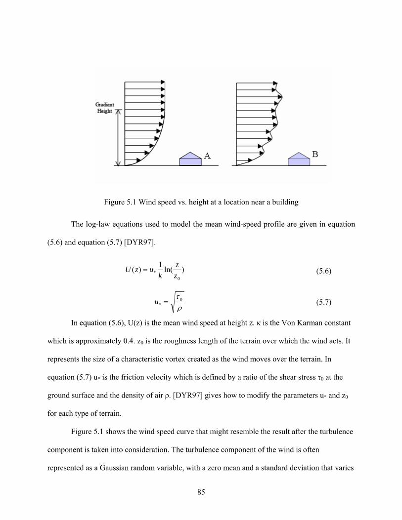
Figure 5.1 Wind speed vs. height at a location near a building
The log-law equations used to model the mean wind-speed profile are given in equation
(5.6) and equation (5.7) [DYR97].
)ln(1)(0
* zz
kuzU = (5.6)
ρτ 0
* =u (5.7)
In equation (5.6), U(z) is the mean wind speed at height z. κ is the Von Karman constant
which is approximately 0.4. z0 is the roughness length of the terrain over which the wind acts. It
represents the size of a characteristic vortex created as the wind moves over the terrain. In
equation (5.7) u* is the friction velocity which is defined by a ratio of the shear stress τ0 at the
ground surface and the density of air ρ. [DYR97] gives how to modify the parameters u* and z0
for each type of terrain.
Figure 5.1 shows the wind speed curve that might resemble the result after the turbulence
component is taken into consideration. The turbulence component of the wind is often
represented as a Gaussian random variable, with a zero mean and a standard deviation that varies
85
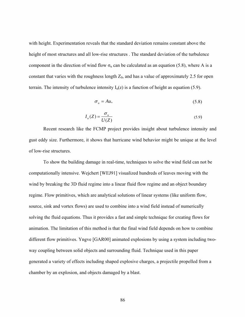
with height. Experimentation reveals that the standard deviation remains constant above the
height of most structures and all low-rise structures . The standard deviation of the turbulence
component in the direction of wind flow σu can be calculated as an equation (5.8), where A is a
constant that varies with the roughness length Z0, and has a value of approximately 2.5 for open
terrain. The intensity of turbulence intensity Iu(z) is a function of height as equation (5.9).
*Auu =σ (5.8)
)()(
ZUZI u
uσ
= (5.9)
Recent research like the FCMP project provides insight about turbulence intensity and
gust eddy size. Furthermore, it shows that hurricane wind behavior might be unique at the level
of low-rise structures.
To show the building damage in real-time, techniques to solve the wind field can not be
computationally intensive. Wejchert [WEJ91] visualized hundreds of leaves moving with the
wind by breaking the 3D fluid regime into a linear fluid flow regime and an object boundary
regime. Flow primitives, which are analytical solutions of linear systems (like uniform flow,
source, sink and vortex flows) are used to combine into a wind field instead of numerically
solving the fluid equations. Thus it provides a fast and simple technique for creating flows for
animation. The limitation of this method is that the final wind field depends on how to combine
different flow primitives. Yngve [GAR00] animated explosions by using a system including two-
way coupling between solid objects and surrounding fluid. Technique used in this paper
generated a variety of effects including shaped explosive charges, a projectile propelled from a
chamber by an explosion, and objects damaged by a blast.
86
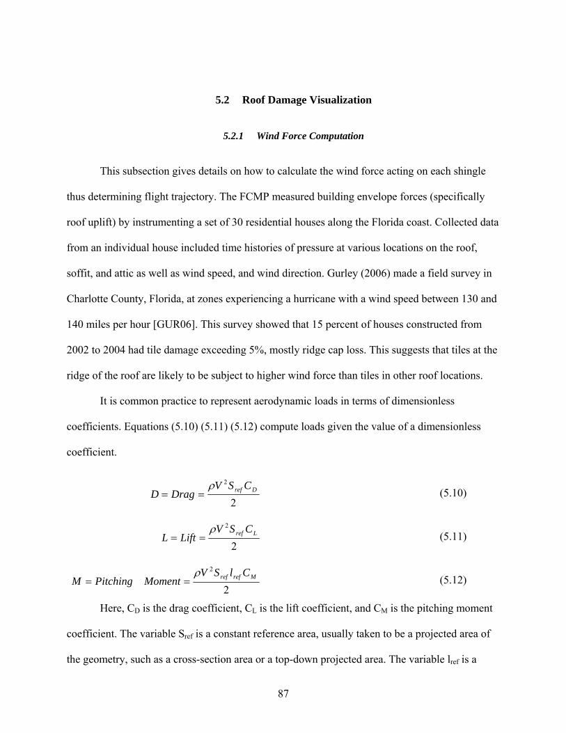
5.2 Roof Damage Visualization
5.2.1 Wind Force Computation
This subsection gives details on how to calculate the wind force acting on each shingle
thus determining flight trajectory. The FCMP measured building envelope forces (specifically
roof uplift) by instrumenting a set of 30 residential houses along the Florida coast. Collected data
from an individual house included time histories of pressure at various locations on the roof,
soffit, and attic as well as wind speed, and wind direction. Gurley (2006) made a field survey in
Charlotte County, Florida, at zones experiencing a hurricane with a wind speed between 130 and
140 miles per hour [GUR06]. This survey showed that 15 percent of houses constructed from
2002 to 2004 had tile damage exceeding 5%, mostly ridge cap loss. This suggests that tiles at the
ridge of the roof are likely to be subject to higher wind force than tiles in other roof locations.
It is common practice to represent aerodynamic loads in terms of dimensionless
coefficients. Equations (5.10) (5.11) (5.12) compute loads given the value of a dimensionless
coefficient.
2
2Dref CSV
DragDρ
== (5.10)
2
2Lref CSV
LiftLρ
== (5.11)
2
2Mrefref ClSV
MomentPitchingMρ
== (5.12)
Here, CD is the drag coefficient, CL is the lift coefficient, and CM is the pitching moment
coefficient. The variable Sref is a constant reference area, usually taken to be a projected area of
the geometry, such as a cross-section area or a top-down projected area. The variable lref is a
87
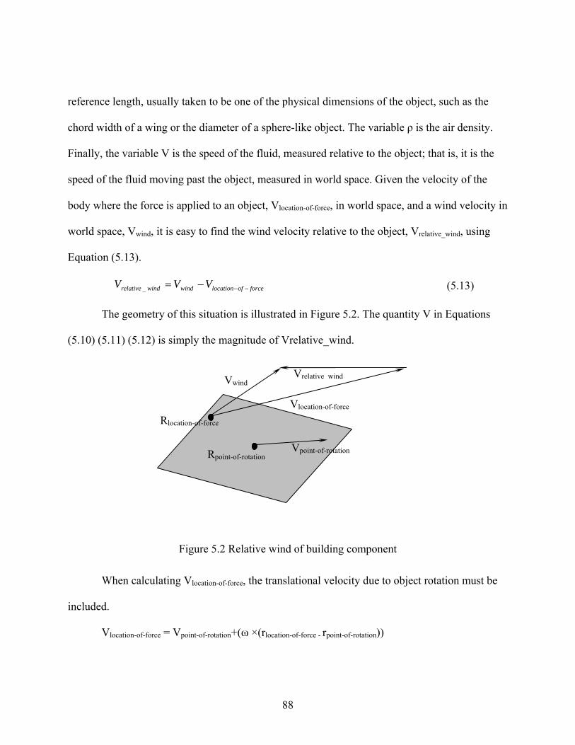
reference length, usually taken to be one of the physical dimensions of the object, such as the
chord width of a wing or the diameter of a sphere-like object. The variable ρ is the air density.
Finally, the variable V is the speed of the fluid, measured relative to the object; that is, it is the
speed of the fluid moving past the object, measured in world space. Given the velocity of the
body where the force is applied to an object, Vlocation-of-force, in world space, and a wind velocity in
world space, Vwind, it is easy to find the wind velocity relative to the object, Vrelative_wind, using
Equation (5.13).
forceoflocationwindwindrelative VVV −−−=_ (5.13)
The geometry of this situation is illustrated in Figure 5.2. The quantity V in Equations
(5.10) (5.11) (5.12) is simply the magnitude of Vrelative_wind.
Vlocation-of-force
VwindVrelative wind
Rlocation-of-force
Rpoint-of-rotationVpoint-of-rotation
Figure 5.2 Relative wind of building component
When calculating Vlocation-of-force, the translational velocity due to object rotation must be
included.
Vlocation-of-force = Vpoint-of-rotation+(ω ×(rlocation-of-force - rpoint-of-rotation))
88
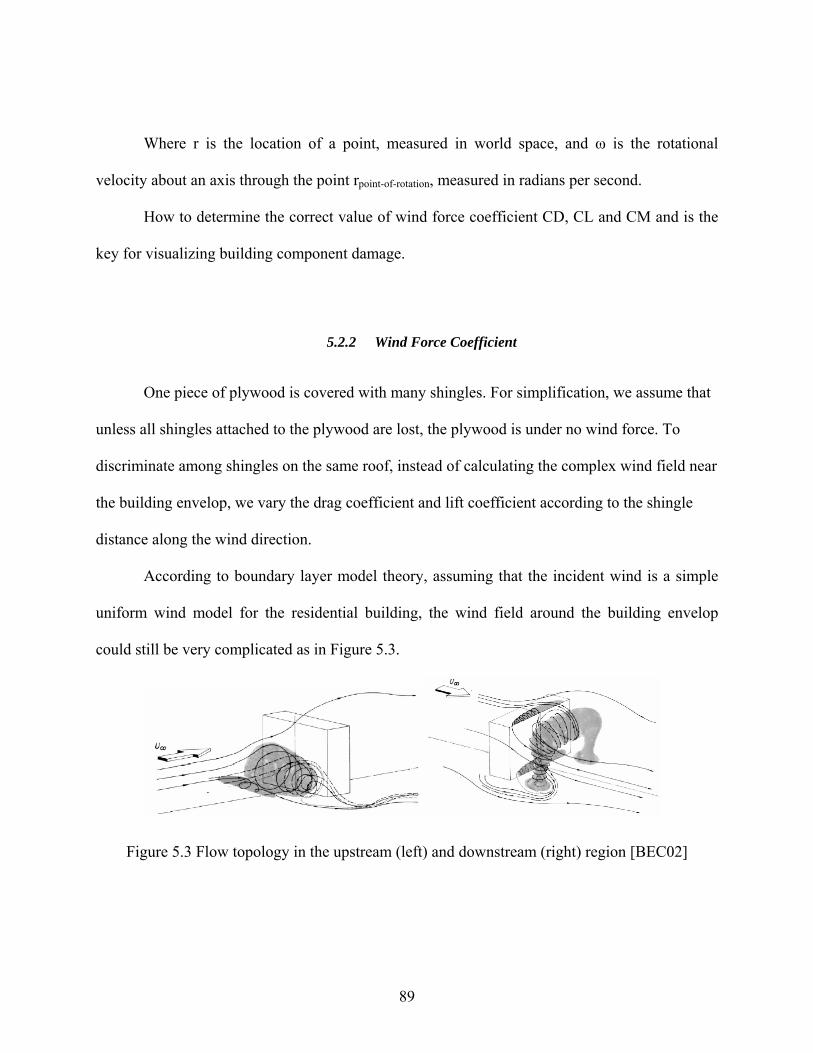
Where r is the location of a point, measured in world space, and ω is the rotational
velocity about an axis through the point rpoint-of-rotation, measured in radians per second.
How to determine the correct value of wind force coefficient CD, CL and CM and is the
key for visualizing building component damage.
5.2.2 Wind Force Coefficient
One piece of plywood is covered with many shingles. For simplification, we assume that
unless all shingles attached to the plywood are lost, the plywood is under no wind force. To
discriminate among shingles on the same roof, instead of calculating the complex wind field near
the building envelop, we vary the drag coefficient and lift coefficient according to the shingle
distance along the wind direction.
According to boundary layer model theory, assuming that the incident wind is a simple
uniform wind model for the residential building, the wind field around the building envelop
could still be very complicated as in Figure 5.3.
Figure 5.3 Flow topology in the upstream (left) and downstream (right) region [BEC02]
89
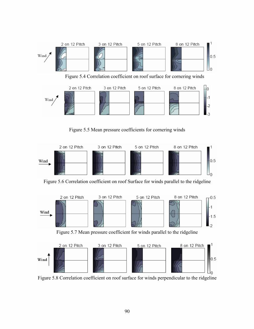
Figure 5.4 Correlation coefficient on roof surface for cornering winds
Figure 5.5 Mean pressure coefficients for cornering winds
Figure 5.6 Correlation coefficient on roof Surface for winds parallel to the ridgeline
Figure 5.7 Mean pressure coefficient for winds parallel to the ridgeline
Figure 5.8 Correlation coefficient on roof surface for winds perpendicular to the ridgeline
90
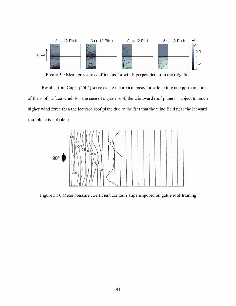
Figure 5.9 Mean pressure coefficients for winds perpendicular to the ridgeline
Results from Cope. (2005) serve as the theoretical basis for calculating an approximation
of the roof surface wind. For the case of a gable roof, the windward roof plane is subject to much
higher wind force than the leeward roof plane due to the fact that the wind field near the leeward
roof plane is turbulent.
Figure 5.10 Mean pressure coefficient contours superimposed on gable roof framing
91
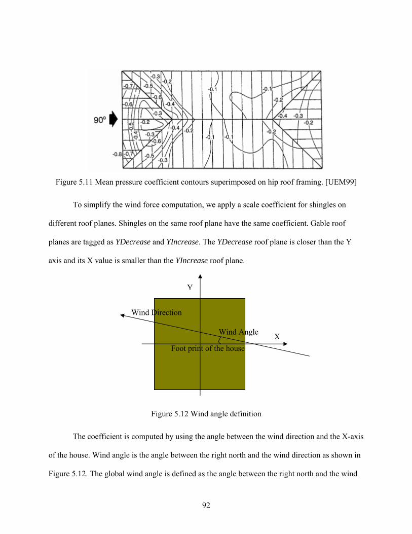
Figure 5.11 Mean pressure coefficient contours superimposed on hip roof framing. [UEM99]
To simplify the wind force computation, we apply a scale coefficient for shingles on
different roof planes. Shingles on the same roof plane have the same coefficient. Gable roof
planes are tagged as YDecrease and YIncrease. The YDecrease roof plane is closer than the Y
axis and its X value is smaller than the YIncrease roof plane.
X
Y
Foot print of the house
Wind Direction
Wind Angle
Figure 5.12 Wind angle definition
The coefficient is computed by using the angle between the wind direction and the X-axis
of the house. Wind angle is the angle between the right north and the wind direction as shown in
Figure 5.12. The global wind angle is defined as the angle between the right north and the wind
92
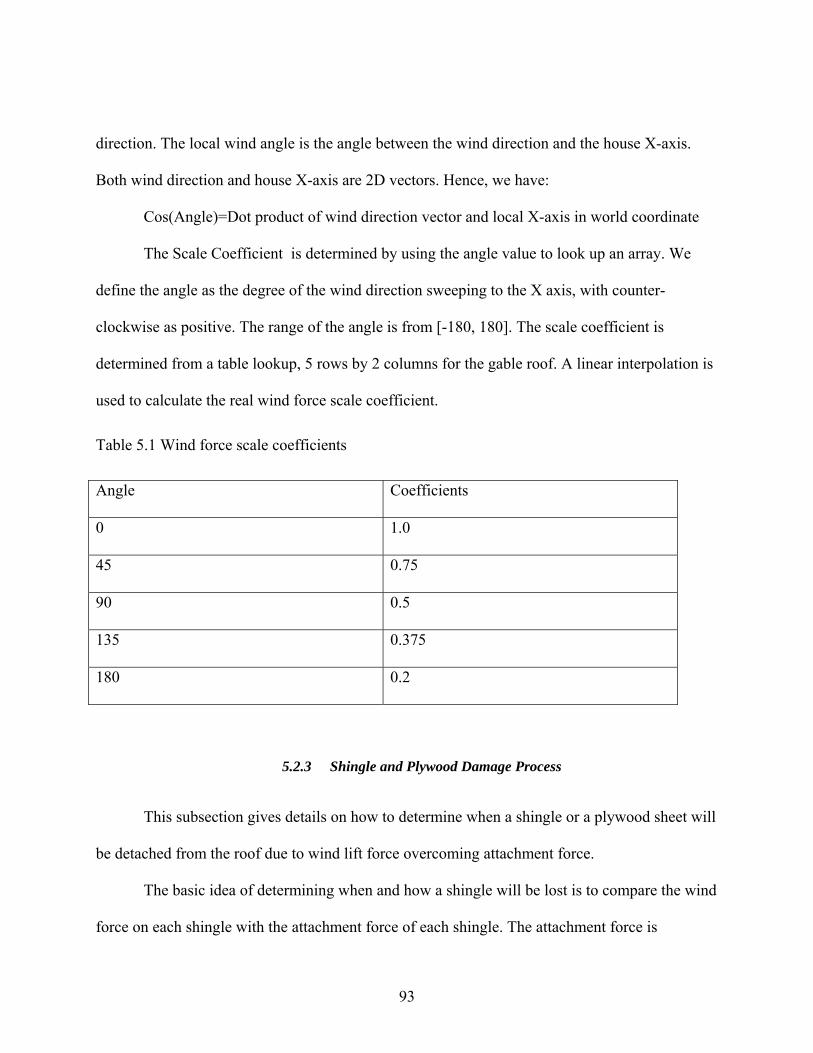
direction. The local wind angle is the angle between the wind direction and the house X-axis.
Both wind direction and house X-axis are 2D vectors. Hence, we have:
Cos(Angle)=Dot product of wind direction vector and local X-axis in world coordinate
The Scale Coefficient is determined by using the angle value to look up an array. We
define the angle as the degree of the wind direction sweeping to the X axis, with counter-
clockwise as positive. The range of the angle is from [-180, 180]. The scale coefficient is
determined from a table lookup, 5 rows by 2 columns for the gable roof. A linear interpolation is
used to calculate the real wind force scale coefficient.
Table 5.1 Wind force scale coefficients
Angle Coefficients
0 1.0
45 0.75
90 0.5
135 0.375
180 0.2
5.2.3 Shingle and Plywood Damage Process
This subsection gives details on how to determine when a shingle or a plywood sheet will
be detached from the roof due to wind lift force overcoming attachment force.
The basic idea of determining when and how a shingle will be lost is to compare the wind
force on each shingle with the attachment force of each shingle. The attachment force is
93
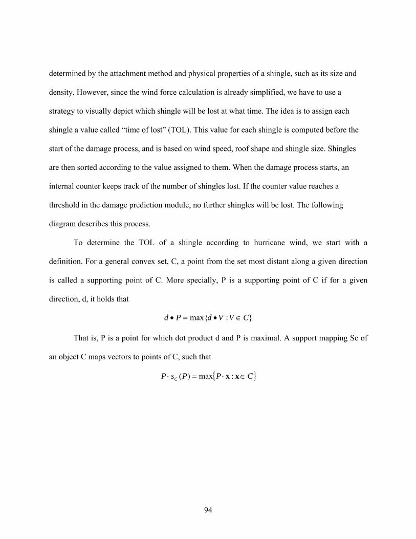
determined by the attachment method and physical properties of a shingle, such as its size and
density. However, since the wind force calculation is already simplified, we have to use a
strategy to visually depict which shingle will be lost at what time. The idea is to assign each
shingle a value called “time of lost” (TOL). This value for each shingle is computed before the
start of the damage process, and is based on wind speed, roof shape and shingle size. Shingles
are then sorted according to the value assigned to them. When the damage process starts, an
internal counter keeps track of the number of shingles lost. If the counter value reaches a
threshold in the damage prediction module, no further shingles will be lost. The following
diagram describes this process.
To determine the TOL of a shingle according to hurricane wind, we start with a
definition. For a general convex set, C, a point from the set most distant along a given direction
is called a supporting point of C. More specially, P is a supporting point of C if for a given
direction, d, it holds that
}:max{ CVVdPd ∈•=•
That is, P is a point for which dot product d and P is maximal. A support mapping Sc of
an object C maps vectors to points of C, such that
{ }CPPsP C ∈⋅=⋅ xx :max)(
94
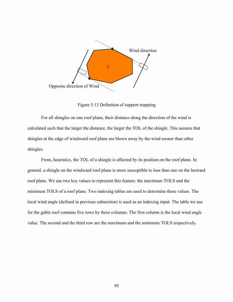
C
Wind direction
Opposite direction of Wind
Figure 5.13 Definition of support mapping
For all shingles on one roof plane, their distance along the direction of the wind is
calculated such that the larger the distance, the larger the TOL of the shingle. This assures that
shingles at the edge of windward roof plane are blown away by the wind sooner than other
shingles.
From, heuristics, the TOL of a shingle is affected by its position on the roof plane. In
general, a shingle on the windward roof plane is more susceptible to loss than one on the leeward
roof plane. We use two key values to represent this feature: the maximum TOLS and the
minimum TOLS of a roof plane. Two indexing tables are used to determine these values. The
local wind angle (defined in previous subsection) is used as an indexing input. The table we use
for the gable roof contains five rows by three columns. The first column is the local wind angle
value. The second and the third row are the maximum and the minimum TOLS respectively.
95
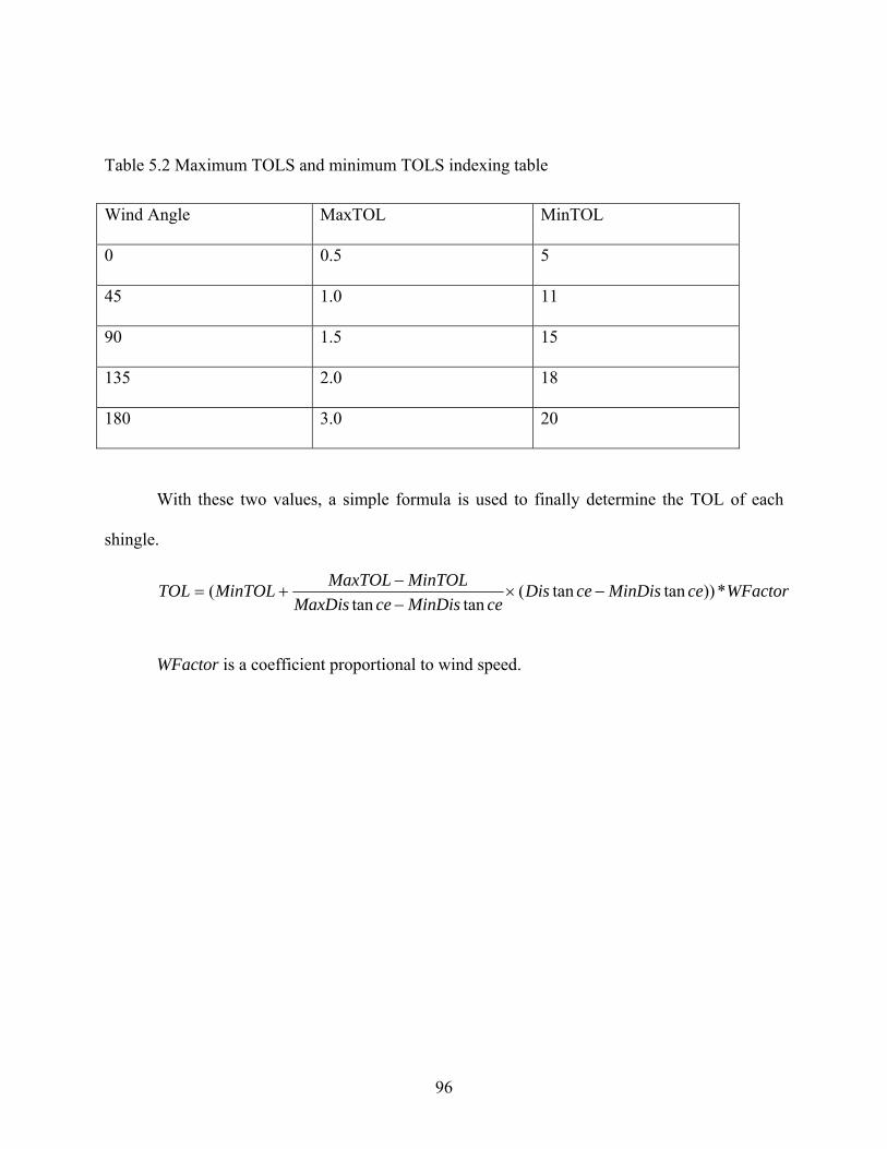
Table 5.2 Maximum TOLS and minimum TOLS indexing table
Wind Angle MaxTOL MinTOL
0 0.5 5
45 1.0 11
90 1.5 15
135 2.0 18
180 3.0 20
With these two values, a simple formula is used to finally determine the TOL of each
shingle.
WFactorceMinDisceDisceMinDisceMaxDis
MinTOLMaxTOLMinTOLTOL *))tantan(tantan
( −×−−
+=
WFactor is a coefficient proportional to wind speed.
96
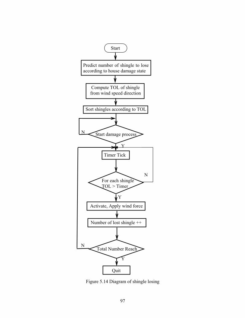
Number of lost shingle ++
N
Y
Activate, Apply wind force
Sort shingles according to TOL
Start
Predict number of shingle to lose according to house damage state
Compute TOL of shingle from wind speed direction
Start damage process
Timer Tick
For each shingle TOL > Timer
Total Number Reach
Quit
N
Y
N
Y
Figure 5.14 Diagram of shingle losing
97
5.3 Wall and Opening Damage Visualization
The masonry wall damage process is simplified such that force is applied to each brick
eventually which can lead to the wall collapsing, given enough force. Once a breach is detected,
we apply forces on the four walls. The direction of forces is the external normal of the wall
plane.
However, wooden walls and openings are subject to breaking in a hurricane. Damage of
wooden walls and openings are common in that cracks and holes appear due to external forces.
Objects with holes or cracks must therefore be subdivided into simple convex polygons before
they can be rendered. Wooden walls or window glass break and fracture can be triggered by two
factors: Pressure force which exceeds building component capacity; and strong collision impact.
[JOH04] uses both finite elements and meshless particles to compute projectile impact
on a multi-plate target. The object is initially made up of elements and the deformation process is
solved by finite element analysis. As the solution progresses, the highly strained finite elements
are converted into meshless particles. This method combines the benefits of both finite elements
and meshless particles. The use of finite elements allows for an accurate and efficient solution
for the less distorted portion of the object. Meshless particles can accurately and robustly model
highly deformation-induced fracture. Terzopoulos and Fleischer [TER88] presented a general
technique for modeling viscoelastic and plastic deformations. Energy functions are defined using
three fundamental metric tensors that measure deformation over curves, surfaces, and volumes.
The continuous deformation model based on the energy functions are made discrete by a finite
differencing technique which is defined by controlled continuity splines [TER86]. If setting the
elastic coefficients between adjacent nodes to zero whenever the distance between the nodes
98
exceeded a threshold, certain fracture effects can be modeled. Norton [NOR91] presented a
technique for animating 3D solid objects that break when subjected to large strains. Consider
what modeling processes are needed to depict a teapot shattering. A spring-mass system is used
to model this behavior. When the distance between two attached mass points exceed a threshold,
the simulation severs the spring connection between them. O’ Brien (1999) pointed out two
limitations of these two methods. First, when the material fails, the exact location and orientation
of the fracture are not known. As a result, these techniques can only realistically model effects
that occur on a scale much larger than the inter-node spacing.
Apparently, research done in the area of the fracturing of brittle materials is generally not
published because of the fact that the underlying physics have been simplified in such a way that
they can be used in interactive simulation. Therefore, we have based our algorithm on
observations, intuition and some basic knowledge of breaking of glass found online.
Glass (SiO2) is an amorphous material, which has properties of both a solid and a fluid.
On a microscopic level, Its atoms do not lie in straight lines but are arranged somewhat
randomly. Therefore, it is almost impossible to describe exactly how a crack will propagate.
However, it is reasonable to conclude that a crack will continue in the same direction as it
started. Whether the window glass will crack at all depends on the force of the impact. The
Weibull distribution, approximates the probability of cracks forming for a given input stress
[ASK96]. Glass has a Weibull number of 5-8. Low numbers implying a wider distribution (steel
has a Weibull number of about 40). A window will withstand a harder impact in the middle of
the glass than at the edges. This is because, at the edges the glass is fixed to a frame and
therefore it cannot flex as freely as in the center, thus breaking more easily when subject to a
99
given force. When glass is formed, tiny air bubbles are also formed. When a crack comes to an
air bubble, its behavior is undefined; it can change direction completely, divide itself into several
new cracks or perhaps stop completely. This is because the crack will continue in the direction
where the “edges” in the air bubble are the weakest, and there may be several such spots. The
number of air bubbles in a glass is impossible to tell in advance, but if there are visible ones,
there are probably many more that are so small that they cannot be seen with the naked eye. A
crack propagates at very high speed. This differs with different kinds of glass, but in general the
speed is approximately 1950 m/s [WEE04], compared to a bullet that travels at about 800 m/s.
This means that you will never be able to see a crack spread in a window glass. When a strike
hits a window, cracks will form if the glass bends more than it can withstand. Glass as a material
is non-elastic, which is why a window easily cracks. If a strike is hard enough, circumferential
crack patterns will form. Also, the number of radial cracks will be larger [MEN02]. There is no
way of telling how many cracks will form when the window is hit by a given blow, but in
general you can say that if you hit harder, more cracks will form. There will almost always be
cracks forming at opposite directions from each other, i.e. if one crack propagates out from the
impact point at one direction there will be another that starts off with the angle of the other one
plus 180 degrees. When you hit hard enough the holes in the window will no longer get larger,
but smaller. This is because the object you hit with will go through the glass before it has time to
expose the material to any significant amount of bending stress. This also means that the cracks
that form become shorter [MEN02]. That is why there can be small holes of sizes almost equal to
the bullets’ when certain types of glass windows have been shot. A glass that already has cracks
100
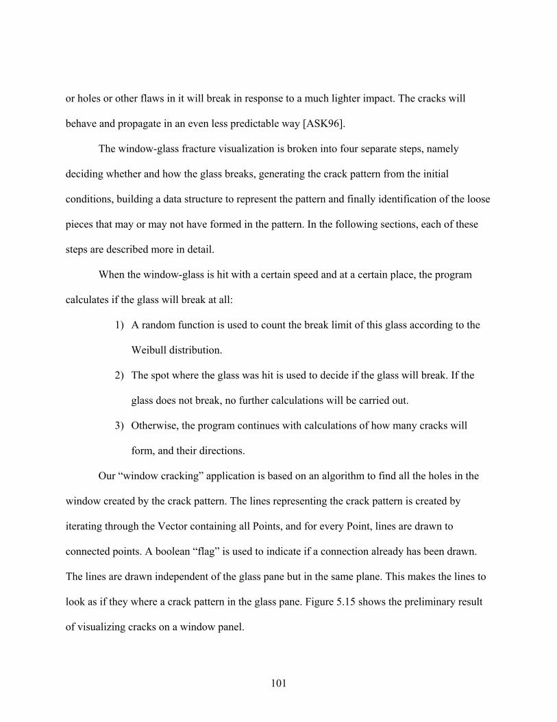
or holes or other flaws in it will break in response to a much lighter impact. The cracks will
behave and propagate in an even less predictable way [ASK96].
The window-glass fracture visualization is broken into four separate steps, namely
deciding whether and how the glass breaks, generating the crack pattern from the initial
conditions, building a data structure to represent the pattern and finally identification of the loose
pieces that may or may not have formed in the pattern. In the following sections, each of these
steps are described more in detail.
When the window-glass is hit with a certain speed and at a certain place, the program
calculates if the glass will break at all:
1) A random function is used to count the break limit of this glass according to the
Weibull distribution.
2) The spot where the glass was hit is used to decide if the glass will break. If the
glass does not break, no further calculations will be carried out.
3) Otherwise, the program continues with calculations of how many cracks will
form, and their directions.
Our “window cracking” application is based on an algorithm to find all the holes in the
window created by the crack pattern. The lines representing the crack pattern is created by
iterating through the Vector containing all Points, and for every Point, lines are drawn to
connected points. A boolean “flag” is used to indicate if a connection already has been drawn.
The lines are drawn independent of the glass pane but in the same plane. This makes the lines to
look as if they where a crack pattern in the glass pane. Figure 5.15 shows the preliminary result
of visualizing cracks on a window panel.
101
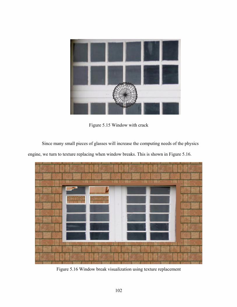
Figure 5.15 Window with crack
Since many small pieces of glasses will increase the computing needs of the physics
engine, we turn to texture replacing when window breaks. This is shown in Figure 5.16.
Figure 5.16 Window break visualization using texture replacement
102

5.4 Damage Rule Incorporation
The first damage rule is the damage prediction result. A physical damage model show as
Figure 5.17 is used in HAZUS®. It predicts wind-induced pressure damage to openings, wall
cladding, roof cladding, roof cover and connections. This model compares loads to resistances to
determine hurricane-induced building damage. Both masonry and wood frame wall failures are
due to inward and outward pressure loads, which are modeled. Failure of the connections
between the roof frame and the perimeter walls are modeled for wood and steel roof framing
systems. The inherent nature of this computation is Monte Carlo simulation. The output is
statistical, i.e. it is based on the probability of certain kinds of damage. Hence this model can not
be used in our hurricane visualization which is an interactive simultion.
We come up with a simple database containing engineering data from the HAZUS®
software program. The database assisted design also lead to a feature that changing the database
will changing the damage prediction result.
103
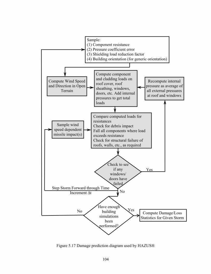
Compare computed loads for resistances Check for debris impact Fall all components where load exceeds resistance Check for structural failure of roofs, walls, etc., as required
Sample: (1) Component resistance (2) Pressure coefficient error (3) Shielding load reduction factor (4) Building orientation (for generic orientation)
No
Yes
Compute component and cladding loads on roof cover, roof sheathing, windows, doors, etc. Add internal pressures to get total loads
Compute Wind Speed and Direction in Open
Terrain
Check to see if any
windows/ doors have
failed
No
Recompute internal pressure as average of all external pressures at roof and windows
Sample wind speed dependent missile impact(s)
Have enough building
simulations been
performed?
Step Storm Forward through Time Increment ∆t
YesCompute Damage/Loss
Statistics for Given Storm
Figure 5.17 Damage prediction diagram used by HAZUS®
104

The whole building damage state is a combination of damage states of five types of
building components: roof cover, roof shealth, truss, opening and wall. Table 5.3 defines
building component damage according to its whole building damage state. This is the second
damage rule we use in the visualization system.The damage state of each building component
governs the visualization details including motion, breaking, and fracture of different type of
building components.
Table 5.3 Damage state for residential buildings defined in HAZUS®
Damage
State
Qualitative Damage Description Roof
Cover
Failure
Window
Door
Failures
Roof
Deck
Missile
Impacts
on Walls
Roof
Failure
Wall
Failure
0 No Damage or Very Minor Damages
Little or no visible damage from the
outside. No broken widows, or failed
roof deck. Minimal loss of roof cover,
with no or very limited water penetration
<2% No No No No No
1 Minor Damage
Maximum of one broken window, door
or garage door. Moderate roof cover loss
that can be covered to prevent additional
water entering the building. Marks or
dents on walls requiring painting or
patching for repair.
>2% and
<15%
One
window,
door, or
garage
door
failure
No <5
impacts
No No
2 Moderate damage
Major roof cover damage, minor roof
sheathing failure. Some resulting
damage to the interior of building from
water
>15%
and
<50%
>One
item &
up to
20%
overall
damage
1 to 3
panels
Typically
5 to 10
impacts
No No
105
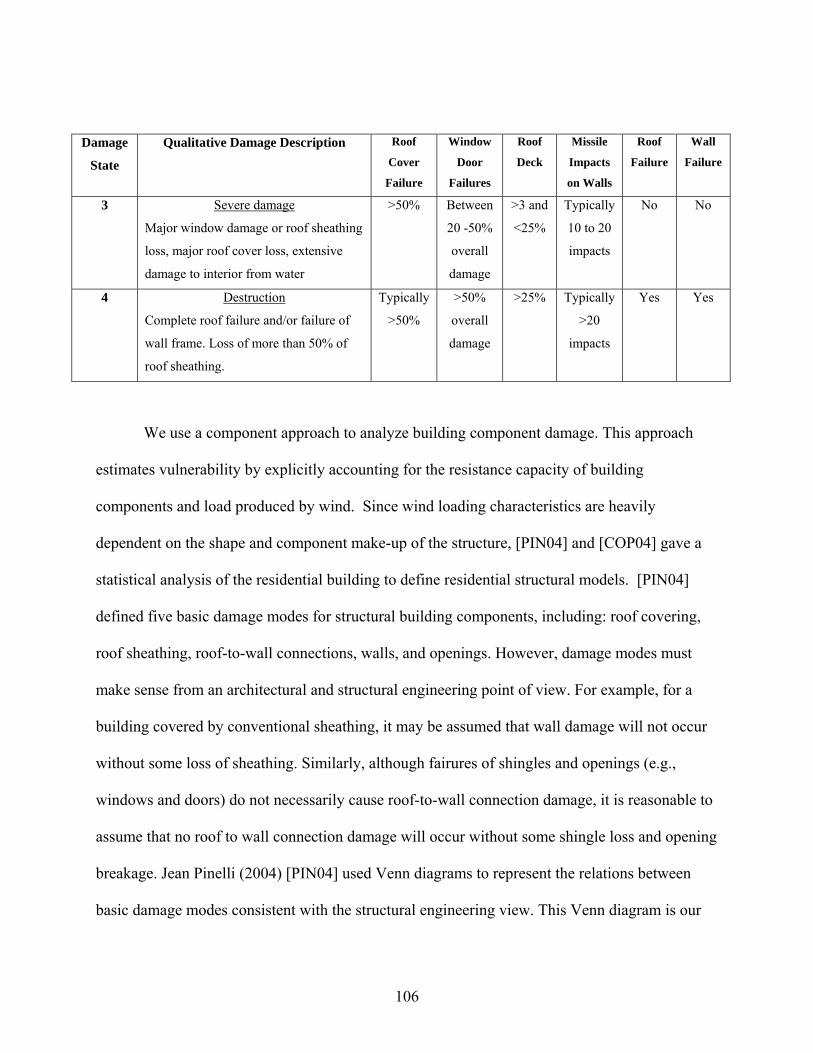
Damage
State
Qualitative Damage Description Roof
Cover
Failure
Window
Door
Failures
Roof
Deck
Missile
Impacts
on Walls
Roof
Failure
Wall
Failure
3 Severe damage
Major window damage or roof sheathing
loss, major roof cover loss, extensive
damage to interior from water
>50% Between
20 -50%
overall
damage
>3 and
<25%
Typically
10 to 20
impacts
No No
4 Destruction
Complete roof failure and/or failure of
wall frame. Loss of more than 50% of
roof sheathing.
Typically
>50%
>50%
overall
damage
>25% Typically
>20
impacts
Yes Yes
We use a component approach to analyze building component damage. This approach
estimates vulnerability by explicitly accounting for the resistance capacity of building
components and load produced by wind. Since wind loading characteristics are heavily
dependent on the shape and component make-up of the structure, [PIN04] and [COP04] gave a
statistical analysis of the residential building to define residential structural models. [PIN04]
defined five basic damage modes for structural building components, including: roof covering,
roof sheathing, roof-to-wall connections, walls, and openings. However, damage modes must
make sense from an architectural and structural engineering point of view. For example, for a
building covered by conventional sheathing, it may be assumed that wall damage will not occur
without some loss of sheathing. Similarly, although fairures of shingles and openings (e.g.,
windows and doors) do not necessarily cause roof-to-wall connection damage, it is reasonable to
assume that no roof to wall connection damage will occur without some shingle loss and opening
breakage. Jean Pinelli (2004) [PIN04] used Venn diagrams to represent the relations between
basic damage modes consistent with the structural engineering view. This Venn diagram is our
106

third damage rule. Table 5.4 shows the tabulated Venn Diagram which is more convenient to
represent in computer software.
107
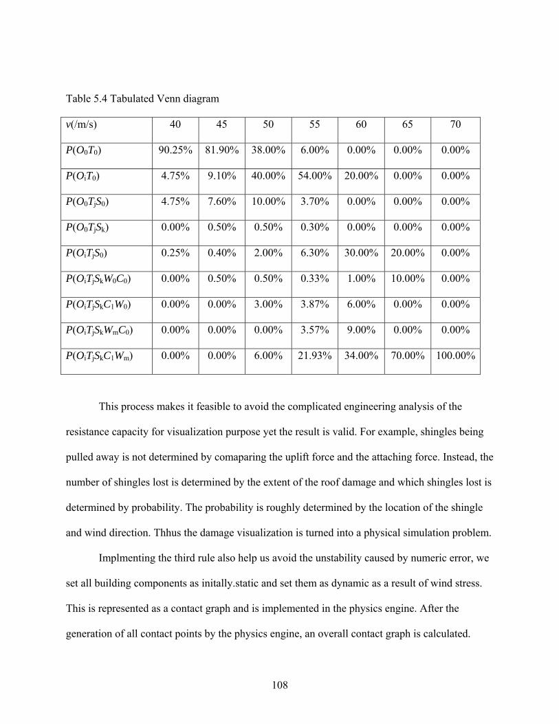
Table 5.4 Tabulated Venn diagram
v(/m/s) 40 45 50 55 60 65 70
P(O0T0) 90.25% 81.90% 38.00% 6.00% 0.00% 0.00% 0.00%
P(OiT0) 4.75% 9.10% 40.00% 54.00% 20.00% 0.00% 0.00%
P(O0TjS0) 4.75% 7.60% 10.00% 3.70% 0.00% 0.00% 0.00%
P(O0TjSk) 0.00% 0.50% 0.50% 0.30% 0.00% 0.00% 0.00%
P(OiTjS0) 0.25% 0.40% 2.00% 6.30% 30.00% 20.00% 0.00%
P(OiTjSkW0C0) 0.00% 0.50% 0.50% 0.33% 1.00% 10.00% 0.00%
P(OiTjSkC1W0) 0.00% 0.00% 3.00% 3.87% 6.00% 0.00% 0.00%
P(OiTjSkWmC0) 0.00% 0.00% 0.00% 3.57% 9.00% 0.00% 0.00%
P(OiTjSkC1Wm) 0.00% 0.00% 6.00% 21.93% 34.00% 70.00% 100.00%
This process makes it feasible to avoid the complicated engineering analysis of the
resistance capacity for visualization purpose yet the result is valid. For example, shingles being
pulled away is not determined by comaparing the uplift force and the attaching force. Instead, the
number of shingles lost is determined by the extent of the roof damage and which shingles lost is
determined by probability. The probability is roughly determined by the location of the shingle
and wind direction. Thhus the damage visualization is turned into a physical simulation problem.
Implmenting the third rule also help us avoid the unstability caused by numeric error, we
set all building components as initally.static and set them as dynamic as a result of wind stress.
This is represented as a contact graph and is implemented in the physics engine. After the
generation of all contact points by the physics engine, an overall contact graph is calculated.
108
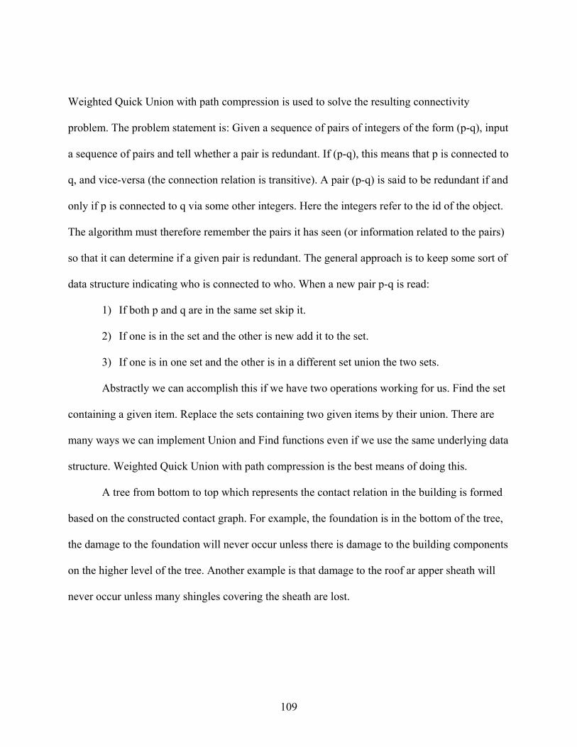
Weighted Quick Union with path compression is used to solve the resulting connectivity
problem. The problem statement is: Given a sequence of pairs of integers of the form (p-q), input
a sequence of pairs and tell whether a pair is redundant. If (p-q), this means that p is connected to
q, and vice-versa (the connection relation is transitive). A pair (p-q) is said to be redundant if and
only if p is connected to q via some other integers. Here the integers refer to the id of the object.
The algorithm must therefore remember the pairs it has seen (or information related to the pairs)
so that it can determine if a given pair is redundant. The general approach is to keep some sort of
data structure indicating who is connected to who. When a new pair p-q is read:
1) If both p and q are in the same set skip it.
2) If one is in the set and the other is new add it to the set.
3) If one is in one set and the other is in a different set union the two sets.
Abstractly we can accomplish this if we have two operations working for us. Find the set
containing a given item. Replace the sets containing two given items by their union. There are
many ways we can implement Union and Find functions even if we use the same underlying data
structure. Weighted Quick Union with path compression is the best means of doing this.
A tree from bottom to top which represents the contact relation in the building is formed
based on the constructed contact graph. For example, the foundation is in the bottom of the tree,
the damage to the foundation will never occur unless there is damage to the building components
on the higher level of the tree. Another example is that damage to the roof ar apper sheath will
never occur unless many shingles covering the sheath are lost.
109
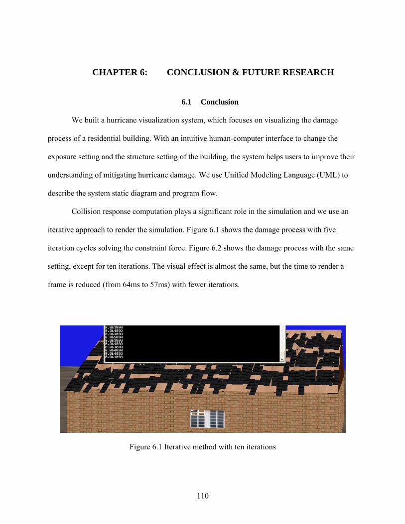
CHAPTER 6: CONCLUSION & FUTURE RESEARCH
6.1 Conclusion
We built a hurricane visualization system, which focuses on visualizing the damage
process of a residential building. With an intuitive human-computer interface to change the
exposure setting and the structure setting of the building, the system helps users to improve their
understanding of mitigating hurricane damage. We use Unified Modeling Language (UML) to
describe the system static diagram and program flow.
Collision response computation plays a significant role in the simulation and we use an
iterative approach to render the simulation. Figure 6.1 shows the damage process with five
iteration cycles solving the constraint force. Figure 6.2 shows the damage process with the same
setting, except for ten iterations. The visual effect is almost the same, but the time to render a
frame is reduced (from 64ms to 57ms) with fewer iterations.
Figure 6.1 Iterative method with ten iterations
110
Figure 6.2 Iterative method with five iterations
In, Figure 6.1 and Figure 6.2, to show the procedural modeling method, both the shingle
size and the plywood size are made smaller than they appeared in previous figures.
Using scalable time for the damage process enables us to visualize hurricane damage
events faster than in real time. Speeding up a slow process results in more interesting, and
therefore better instruction. Figure 6.3 is the visual effect according to a simple equation as
following to determine the TOL of each shingle:
WFactorceMinDisceDisceMinDisceMaxDis
MinTOLMaxTOLMinTOLTOL *))tantan(tantan
( −×−−
+=
By tweaking the TOL calculation such as adding random factor, we get visual effect as
Figure 6.4. A TOL table measured from actual tunnel test should also be able to easily
incorporate into the system.
111
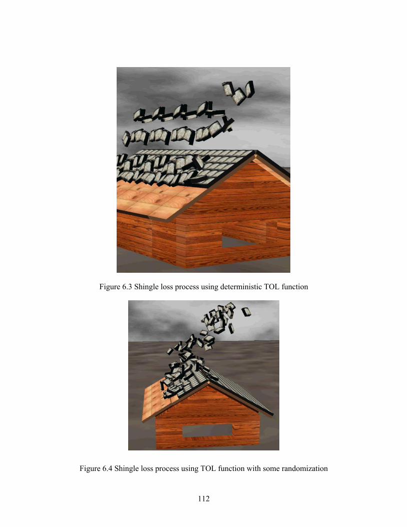
Figure 6.3 Shingle loss process using deterministic TOL function
Figure 6.4 Shingle loss process using TOL function with some randomization
112
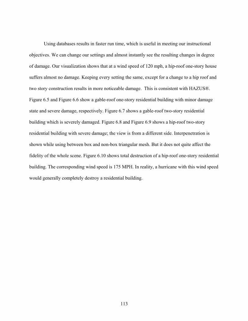
Using databases results in faster run time, which is useful in meeting our instructional
objectives. We can change our settings and almost instantly see the resulting changes in degree
of damage. Our visualization shows that at a wind speed of 120 mph, a hip-roof one-story house
suffers almost no damage. Keeping every setting the same, except for a change to a hip roof and
two story construction results in more noticeable damage. This is consistent with HAZUS®.
Figure 6.5 and Figure 6.6 show a gable-roof one-story residential building with minor damage
state and severe damage, respectively. Figure 6.7 shows a gable-roof two-story residential
building which is severely damaged. Figure 6.8 and Figure 6.9 shows a hip-roof two-story
residential building with severe damage; the view is from a different side. Interpenetration is
shown while using between box and non-box triangular mesh. But it does not quite affect the
fidelity of the whole scene. Figure 6.10 shows total destruction of a hip-roof one-story residential
building. The corresponding wind speed is 175 MPH. In reality, a hurricane with this wind speed
would generally completely destroy a residential building.
113
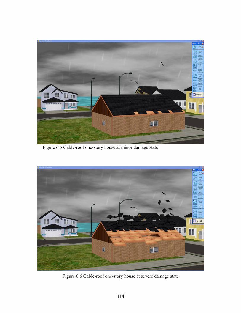
Figure 6.5 Gable-roof one-story house at minor damage state
Figure 6.6 Gable-roof one-story house at severe damage state
114
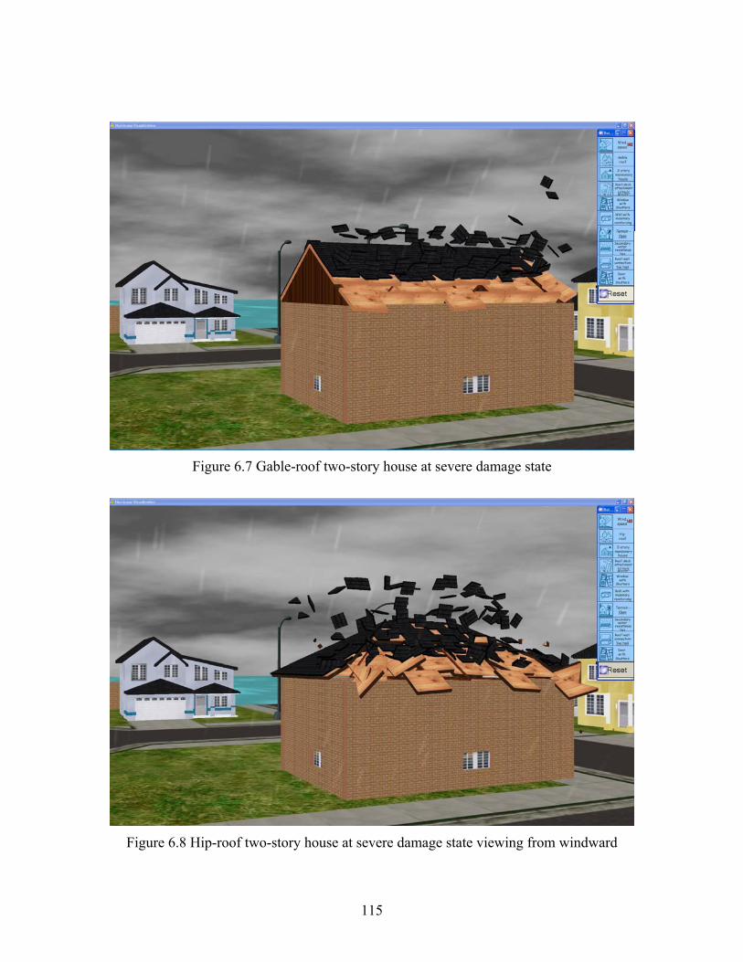
Figure 6.7 Gable-roof two-story house at severe damage state
Figure 6.8 Hip-roof two-story house at severe damage state viewing from windward
115
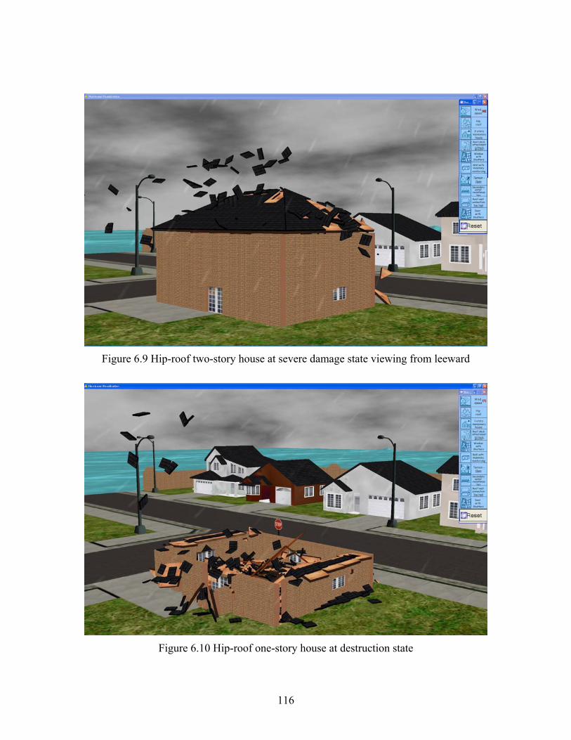
Figure 6.9 Hip-roof two-story house at severe damage state viewing from leeward
Figure 6.10 Hip-roof one-story house at destruction state
116
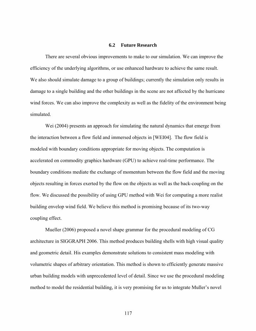
6.2 Future Research
There are several obvious improvements to make to our simulation. We can improve the
efficiency of the underlying algorithms, or use enhanced hardware to achieve the same result.
We also should simulate damage to a group of buildings; currently the simulation only results in
damage to a single building and the other buildings in the scene are not affected by the hurricane
wind forces. We can also improve the complexity as well as the fidelity of the environment being
simulated.
Wei (2004) presents an approach for simulating the natural dynamics that emerge from
the interaction between a flow field and immersed objects in [WEI04]. The flow field is
modeled with boundary conditions appropriate for moving objects. The computation is
accelerated on commodity graphics hardware (GPU) to achieve real-time performance. The
boundary conditions mediate the exchange of momentum between the flow field and the moving
objects resulting in forces exerted by the flow on the objects as well as the back-coupling on the
flow. We discussed the possibility of using GPU method with Wei for computing a more realist
building envelop wind field. We believe this method is promising because of its two-way
coupling effect.
Mueller (2006) proposed a novel shape grammar for the procedural modeling of CG
architecture in SIGGRAPH 2006. This method produces building shells with high visual quality
and geometric detail. His examples demonstrate solutions to consistent mass modeling with
volumetric shapes of arbitrary orientation. This method is shown to efficiently generate massive
urban building models with unprecedented level of detail. Since we use the procedural modeling
method to model the residential building, it is very promising for us to integrate Muller’s novel
117
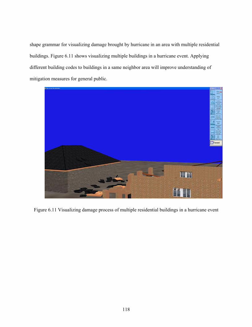
shape grammar for visualizing damage brought by hurricane in an area with multiple residential
buildings. Figure 6.11 shows visualizing multiple buildings in a hurricane event. Applying
different building codes to buildings in a same neighbor area will improve understanding of
mitigation measures for general public.
Figure 6.11 Visualizing damage process of multiple residential buildings in a hurricane event
118
REFERENCES
[AMA00] Amato N.M., Goodrich M.T., and Ramos E.A., 2000, Linear-Time Triangulation of a Simple Polygon Made Easier via Randomization. Proc. 16th Annual. ACM Sympos. Computing Geometry, pp. 201-212.
[AND95] Anderson, T. L. 1995, Fracture Mechanics: Fundamentals and Applications. CRC
Press, Boca Raton, second edition. [BAR89] Baraff, D., 1989, Analytical Methods for Dynamic Simulation of Non-penetrating
Rigid Bodies. Computer Graphics, 23(3):pp. 223-232, July. [BAR96] Baraff, D., 1996, Linear-time Dynamics Using Lagrange Mltipliers. Computer
Graphics Proceedings, Annual Conference Series: pp137-146 [BAR98] Baraff, D. and Witkin, A., 1998, Physically Based Modeling. SIGGRAPH ’98
Course Notes. [BEL03] Belyaev,V., 2003, Real-time simulation of water surface, Graphics Conference
Proceedings. [BEC02] Becker, S., Lienhart, H., 2002, Flow around three-dimensional obstacles in
boundary layers, Journal of Wind Engineering and Industrial Aerodynamics 90 265–279
[BIL00] Billingham, J. and King, A.C., 2000, Wave Motion. Cambridge University Press. [BOS88] Bosco, J. & Wagner, J. 1988, A comparison of the effectiveness of interactive
laser disc and classroom video tape for safety instruction of General Motors workers. Educational Technology, 28(6), 15-22.
[CHO71] Chow, S. H. 1971, A study of windfield in the planetary boundary layer of a
moving tropical cyclone. MS thesis, School of Engineering. and Science, New York University, New York.
[COP04] Cope, A., 2004, Predicting the Vulnerability of typical residential buildings to
hurricane damage. University of Florida PHD thesis. [COP05] Cope, A., Gurley, K., 2005, Low-rise gable roof wind loads: Characterization and
stochastic simulation. Journal of Wind Engineering and Industrial Aerodynamics 93 719–738.
119
[DYR97] Dyrbye, C., Hansen, S. 1997, Wind Loads on Structures, John Wiley & Sons, New York, NY.
[EBE04] Eberly D. 2004, Game Physics, First Edition, Morgan Kaufmann. [FLE90] Fletcher, J. 1990, Effectiveness and cost of interactive videodisc instruction in
defence training and education. IDA Report R2372. Institute for Defence Analysis, Arlington, Va, July.
[FOU84] Fournier A. and Montuno D.Y., 1984, Triangulating Simple Polygons and
Equivalent Problems. ACM Trans. on Graphics (2), pp. 153-174. [GAR00] Gary D. Y., 2000, Animating Explosions. Proceedings of SIGGRAPH, New
York: ACM Press/Addison-Wesley Publishing Co.,29~36. [GIL90] Gilbert, E. G. and Foo, C.P. 1990, Computing the Distance between General
Convex Objects in Three-dimensional Space. IEEE Transactions on Robotics and Automation, 6(1):53–61.
[GUB03] Guendelman, E., Bridson, R. and Fedkiw, R. 2003, Nonconvex Rigid Bodies with
Stacking. ACM Transactions on Graphics, Vol. 22, No.3. [GUR06] Gurley, K. and Davis, R., 2006, Post 2004 Hurricane Field Survey. Proceedings
of the 2006 Structures Congress. [HAR03] Hart, G. D. and Anitescu, M., 2003, A Hard-Constraint Time-Stepping Approach
for Rigid Multibody Dynamics with Joints, Contact, and Friction. TAPIA’03, ACM.
[JIM01] Jiménez, P., Thomas F. and Torras C., 2001, 3D collision detection: a survey.
Computers and Graphics, 25 (2), pp. 269-285, Pergamon Press / Elsevier Science. [KAC03] Kacic-Alesic Z., Nordenstamm M. 2003, A Practical Dynamics System.
Eurographics/SIGGRAPH Symposium on Computer Animation. [LIN05] Lindt, J., 2005, Residential Structures in the Wake of Hurricane Katrina. Found
at: http://www.engr.colostate.edu/~jwv/Preliminary%20Report.pdf. [MAS01] Mason, M., 2001, Mechanics of robotic manipulation. MIT Press. [MIC04] Micikevicius, P., Hughes, C.E., Moshell, J.M., Sims, V.K. and Smith, H., 2004,
Perceptual Evaluation of an Interactive Forest Walk-through. VR Usability Workshop: Designing and Evaluating VR Systems. Nottingham, England, January 22-23.
120
[LEA05] Leatherman, S., 2005, Florida Hurricane Alliance Performance Progress
December Report. http://www.ihrc.fiu.edu/fha/report/AnnualProgressReport_NOAA_013106.pdf.
[MIR00] Mirtich, B. 2000, Timewarp Rigid Body Simulation, SIGGRAPH ’00 Conf. Proc.,
pp. 193-200. [MOO88] Moore, M., Wilhelms, J. 1988, Collision Detection and Response for Computer
Animation. Computer Graphics, 22(4), 289-298, August. [MUL92] Muller, D. & Leonetti, R. 1992, A major technological advancement in training.
Instructional Delivery Systems, July/August. [NOR1] Norton, A., 1991, Animation of fracture by physical modeling. The Visual
Computer, 7:210–217. [ORT96] Ortiz, J., 1996, Simulating Dynamic Environment Effects in an Urban Combat
Situation in Support of TTES, ICSS, & DEMM. Technical report, University of Central Florida
[PIN04] Pinelli, J-P., 2004, A Model to Predict Hurricanes Induced Losses for Residential
Structures. Journal of Structural Engineering, Vol. 130, No. 11. [POW03] Powell, M., 2003, State of Florida Hurricane Loss Projection Model: Atmospheric
science component, Proc., 11th Int. Conf. on Wind Engineering, Texas Tech Univ., Lubbock, Tex.
[QUI94] Quinlan S. 1994, Efficient distance computation between non-convex objects. In
IEEE International Conference on Robotics and Automation, pages 3324-3329.
[SAK99] Sakaguchi, T. and Ohya, J., 1999, Modeling and Animation of Botanical Trees for Interactive Virtual Environments. Proceeding of the ACM Symposium on Virtual Reality Software and Technology, pp.139-146.
[SCH04] Schmidl, H., Walker, N., and Lin, M., 2004, Fast Update of OBB Trees for
Collision Detection between Articulated Bodies. Journal of Graphics Tools. [STA99] Stam, J., 1999, Stable Fluids. Proceedings of the 26th annual conference on
Computer graphics and interactive techniques, Pages: 121 - 128
121
[TAR86] Tarjan, R. E. and Van, C. J., 1986, A Linear-Time Algorithm for Triangulating Simple Polygons. Proceeding 18th Annual ACM Sympos. Theory of Computing, pp. 380-388.
[TES01] Tessendorf, J., 2001, Simulating Ocean Water, SIGGRAPH 2001 Course Notes. [THO96] Thompson, E. F., and Cardone, V. J., 1996, Practical Modeling of Hurricane
Surface Wind Fields. Journal of Waterway, Port, Coastal and Ocean Engineering, Vol. 122, No. 4, ASCE, 122(4), 195–205.
[UEM99] Uematsu, Y., Isyumov, N., 1999, Wind pressures acting on low-rise buildings,
Journal of Wind Engineering and Industrial Aerodynamics 82. [VAN05] VAN J. W., 2005, Damage Assessment of Wood-frame Residential Structures in
the Wake of Hurricane Katrina. Found at: http://www.engr.colostate.edu/~jwv/hurricane-Katrina-woodframe/
[VIC95] Vickery, P. J., and Twisdale, A., 1995, Wind-field and Filling Models for
Hurricane Wind-speed Predictions. Journal of Structure Engineering, ASCE, 121(11), 1700–1709.
[VIC00] Vickery, P.J., Skerlj, et al., 2000, Hurricane Wind Field Model for Use in
Hurricane Simulations. Journal of Structural Engineering, Vol. 126, No. 10. [WAN04] Wang, N. and Wade, B. Rendering Falling Rain and Snow. In ACM SIGGRAPH
2004 Technical Sketches Program, Computer Graphics Proceedings, Annual Conference Series.
[WAT04] Watson, C. and Mark, J., 2004, Insurance Rate Filings and Hurricane Loss
Estimation Models, J. Insurance Regulation, 22, Nr. 3. [WEJ91] Wejchert, J. and Haumann, D., 1991, Animation Aerodynamics. Computer
Graphics, Volume 25, Number 4. [WIT87] Witkin A., Fleischer K. 1987. Energy Constraints on Parameterized Models.
Compuetr Graphics, Vol. 21, No.4.
122