physician concentration and negotiated prices: … concentration and negotiated prices: evidence...
TRANSCRIPT

Physician Concentration and Negotiated Prices:
Evidence from State Law Changes∗
Naomi HausmanHebrew University
Kurt LavettiOhio State University
November 13, 2017
Abstract
We study the relationship between physician market concentration and prices negotiatedbetween physician practices and private insurers. We develop new instrumental variables forchanges in concentration using state-level judicial decisions that change the enforceability of non-compete clauses in physician employment contracts. These law changes alter the organizationalincentives of physicians, causing shocks to the concentration of physician markets. Using twodatabases containing the universe of physician establishments and firms in the US between1996 and 2007, linked to prices negotiated with private insurance companies, we show thatprices fall when physician establishments grow larger but rise when physician firms grow largerconditional on establishment concentration. Our results imply that a 100 point increase in theestablishment-based Herfindahl Index (HHI) causes a 1.3% to 1.7% decline in prices, suggestingthat insurers extract some efficiency gains from larger establishments. In contrast, the samechange in concentration caused by physically distinct establishments negotiating jointly leads toprice increases of 1.0% to 2.0%. The overall effect of a one standard deviation increase in statenon-compete enforceability is a 9.6% increase in average physician prices.
JEL Codes: I11, I18, K31
∗We are grateful to Jay Bhattacharya, Jeff Clemens, Leemore Dafny, Michael Dickstein, Will Dow, Alon Eizenberg,Randy Ellis, Josh Gottlieb, Arthur Lewbel, Ian McCarthy, Jesse Rothstein, and seminar participants at ASHE,Berkeley, Chicago Booth Junior Economics Summit, DOJ, Hebrew University, IDC, LSE, MIT, NBER ProductivityLunch, NBER Summer Institute, Northwestern Kellogg, NYU, Stanford, Tel Aviv University, and UGA for helpfulcomments, to Norman Bishara for sharing legal data, and to Eric Auerbach, Richard Braun, Akina Ikudo, and DavidKrosin for research assistance. This research was conducted while Lavetti was a Robert Wood Johnson FoundationScholar in Health Policy at UC Berkeley, and their support is gratefully acknowledged. Any opinions and conclusionsexpressed herein are those of the authors and do not necessarily represent the views of the U.S. Census Bureau. Allresults have been reviewed to ensure that no confidential information is disclosed. Correspondence: [email protected]
1 Introduction
Physician services account for 20% of all U.S. medical spending, and this component grew even faster
than overall medical spending since 1980.1 Anecdotal evidence suggests that physician practices
have consolidated substantially during the past decade. Rising healthcare spending and concern
over high service prices have led numerous researchers to study the effects of market concentration
on prices, both in health insurance markets (Dafny (2010); Dafny et al. (2012); Ericson and Starc
(2012); Ho and Lee (2016)) and in hospital markets (Gowrisankaran et al. (2014); Gaynor and Vogt
(2003)). However, there is relatively limited causal evidence on the extent to which competition
among physicians affects prices negotiated with insurers. Kleiner et al. (2015) and Dunn and
Shapiro (2014) find evidence consistent with market power, but focus on two specialties and use
primarily cross-sectional variation.2
Two empirical challenges have hindered research on physician prices relative to other segments
of healthcare markets. First, longitudinal data on physician practice sizes linked to prices in private
markets are very difficult to obtain, in contrast to more accessible hospital and insurer data. Second,
there is a basic endogeneity challenge—that market structure may be correlated with unobserved
variation in quality, costs, and demand, for example—which may be further compounded by data
limitations. Empirical methods developed in hospital settings with few providers, such as Ho and
Lee (2016) and Gowrisankaran et al. (2014), require data on costs for each provider in a market,
but similar data are not available for the large number of physician practices in most markets.
In this paper we provide comprehensive evidence on the effects of physician market concentration
on negotiated prices with private insurers, addressing both of these empirical challenges. We
employ two complementary data sets containing the universe of all physician practices in the US
between 1996-2007 to construct measures of physician concentration in a variety of ways. The
Medicare Physician Identification and Eligibility Registry (MPIER) from the Center for Medicare
and Medicaid Services (CMS), which contains all practicing physicians in the US, allows us to
aggregate physicians by practice location and calculate establishment-based and medical specialty-
specific concentration measures. In addition, we use confidential Census Bureau data from the
Longitudinal Business Database (LBD), Economic Censuses (EC), and Business Register (SSEL)
to observe firm-level linkages based on IRS tax IDs and to calculate concentration measures using
payroll and sales data in addition to employment data. We link these concentration measures to
Truven Health Analytics MarketScan data on ambulatory care (non-hospital) prices negotiated
between physicians and a large sample of private commercial insurance companies covering every
state in the US. Together, these data provide a uniquely comprehensive picture of virtually every
physician market nationwide from 1996-2007.
To overcome problems associated with endogenous market structure, we construct new instru-
mental variables using judicial decisions that cause changes to state laws governing the enforcea-
1National Health Expenditure Fact Sheet 2013, CMS2Clemens and Gottlieb (2016) also find evidence consistent with the presence physician market power, although
they do not directly estimate the magnitude of the effect of market structure on prices.
1

bility of non-compete agreements (NCAs), which restrict an employee’s ability to leave a firm and
compete against it. As documented by Bishara (2011), NCA laws vary along seven quantifiable
dimensions across states and over time. We construct a panel of law changes for each of these legal
dimensions for every state between 1991-2009 and trace the effects of these law changes through
changes in organizational incentives, organizational structure, physician market concentration, and
finally to average prices.3
We provide a variety of evidence on the mechanisms through which NCA law changes affect
negotiated prices. We show that the law changes have significant effects on the rate of physician-
establishment job separations. These separations affect the rates of new establishment births and
incumbent establishment deaths, leading to changes in the distribution of establishment sizes. Our
controlled event-study estimates suggest that an average law change increasing NCA enforceability
causes a 165 point decline in the HHI within 2 years. Differences in the nonparametric density
of annual HHI changes in the years following law changes suggest that most of our identifying
variation comes from reductions in concentration in the range of about 100 to 400 HHI points.
We use these law changes, which alter the organization and concentration of physician mar-
kets without directly affecting insurers, as IVs to estimate the effect of concentration on prices.
Our fixed effects specifications control for unobserved heterogeneity across geographic markets as
well as census-division-by-year effects, medical specialty effects, service procedure code effects, and
medical facility type effects. Most importantly, the unique ability in our data to observe both esta-
blishments and firms allows us to estimate the marginal effect on prices of increasing establishment
concentration conditional on firm concentration, and vice versa.
The estimates suggest that changes in HHI have heterogeneous effects on negotiated prices that
depend on the structural nature of the concentration changes. Increases in HHI caused by the
growth of physician establishments lead to negative price effects, while increases in HHI due to the
growth of firms that may have physically distinct establishments cause prices to rise. Specifically,
we find that a 100 point increase in the establishment-based HHI causes a reduction in negotiated
prices of about 1.3% to 1.7% on average. In contrast, the same increase in concentration caused by
firm-level consolidation holding fixed establishment concentration causes prices to increase by 1.0%
to 2.0%.4 OLS specifications imply very small (but statistically significant) positive price effects of
0.02% or less, suggesting that our instruments may reduce substantial endogeneity bias. This fixed
effects OLS estimate is consistent with results from Baker et al. (2014), who find that a 100 point
increase in HHI is associated with 0.08% higher prices on average.5
Taken together, these results suggest that the effects of consolidation on prices depend on a
3NCA law has been used previously as a source of variation in important work by Fallick et al. (2006), Marx etal. (2009), and Garmaise (2009). These papers focus on a few specific law changes (in Michigan, Texas, Florida, andLouisiana) or cross sectional differences (Massachusetts vs. California) rather than using the full panel of judicial lawchanges on all seven legal dimensions and in all U.S. states, as we do. Lavetti et al. (2016) provide evidence fromsurvey data that the use of NCAs in physician employment contracts is very common, with about 45% of primarycare physicians in group practices bound by NCAs.
4We define an establishment as a specific physical practice location, differentiated by mailing addresses. In contrast,firms may own multiple establishments, and we identify firms by IRS tax IDs.
5Baker et al. (2014) use Marketscan price data but estimate market structure using Medicare beneficiaries.
2

tradeoff between the efficiency gains of larger establishments and the increased negotiating power
associated with bargaining as a larger organization. To the extent that larger establishments have
greater bargaining leverage, any consequent positive effect on prices is outweighed by insurers
extracting cost reductions due to economies of scale, resulting in a net negative price effect. These
economies of scale could be due, for example, to shared nursing, laboratory, technological, and
administrative resources among more physicians. However, when practices grow larger through
multi-establishment expansion, the net effect on prices is positive, implying that any economies
of scale from mergers of physically-distinct practices have smaller effects on prices than does the
associated bargaining leverage. The estimate provides a lower bound of the effect of physician firm
size on the ability to negotiate higher prices. Although the changes in consolidation from NCA
laws underlying the local average treatment effect we estimate may differ to some extent from
the margin of variation occurring more broadly in physician markets, our estimates suggest that
price effects come predominantly from the channel of establishment level growth, generating a net
negative relationship between concentration and prices on average.
Our approach to studying this question follows the general structure-conduct-performance
(SCP) approach to estimating effects of market structure on prices (Gaynor et al., (2015)), which
has several well-known concerns. The first is that estimates can be sensitive to assumptions about
market definition, which we address by showing that results are consistent across a range of po-
tential market definitions. A second, but perhaps more fundamental, concern is that without a
structural model to estimate both conduct and performance, the choice of market structure mea-
sures can be arbitrary and potentially inconsistent with firm conduct. For example, choosing HHI
as a market structure measure to estimate performance implies very specific implicit assumptions
about conduct: homogeneous goods and Cournot competition. These assumptions may not be
reasonable in many markets.
Previous studies on the effects of provider consolidation in medical care markets have gene-
rally taken a structural approach to modeling bargaining between hospitals and insurers.6 This
approach allows researchers to identify fundamental parameters like Nash bargaining weights and
consumer willingness to pay, and to evaluate counterfactual scenarios like hypothetical mergers or
entry. However, in the physician setting the same general methodology cannot be applied due to
differences in available data on hospitals versus physicians. In addition, this approach requires
claims data to estimate demand and willingness to pay in a manner that allows for unobserved
quality heterogeneity, but these data are unavailable to us at a national level covering our 12-year
study period.
Our approach is instead to show that the patterns in our results are robust to a wide variety
of market definitions and at least five different measures of market structure, each of which has
different assumptions about firm conduct. The similarity of estimates across these models suggests
that, in our setting, assumptions about firm conduct and market definition are less important than
the endogeneity of market structure measures. Although the parameters we are able to identify
6See Capps et al. (2003), Ho and Lee (2016), and Gowrisankaran et al. (2014).
3

are combinations of the more primitive structural parameters, they still provide meaningful and
intuitive answers to important policy questions.
To facilitate the interpretation of our estimand relative to the underlying theoretical parameters,
we derive a linkage between our empirical model and one particular structural model that assumes
Nash-Bertrand conduct, adapted from the Ho and Lee (2016) bargaining model. The connection to
this model provides a framework for understanding why price effects might be positive at the firm-
level but negative at the establishment level, and why our empirical parameters can be interpreted
as lower bound estimates of the rate at which average costs fall with practice sizes and of the effect
of practice size on network value.
The use of new instruments as a source of exogenous variation in market structure requires
careful attention to the exclusion restriction. A potential concern with our IVs could arise if
practices using NCAs have different cost functions, which could directly alter negotiated prices. In
addition, there could be selection on physician quality into practices that choose to impose NCAs.
We present several pieces of evidence against these concerns based on survey data from Lavetti
et al. (2016), which links information on whether physicians have signed NCA contracts to their
negotiated service prices and a variety of quality measures. We show that there is no statistically or
economically significant difference in the prices negotiated between insurers and physician practices
that use NCAs relative to practices of the same size in the same geographic market that do not (the
decision to impose NCAs is made at the firm level, not the physician level).7 Second, there is no
evidence of quality differences associated with the use of NCAs. In addition to a lack of difference
in negotiated prices, which suggests no difference in average quality, physicians with NCAs respond
identically to vignette-based questions designed by clinical experts to elicit knowledge of best-
practices, diagnostic skill, treatment patterns, and clinical recommendations. There is also no
difference in the amount of prior experience that physicians have when entering NCA vs. non-NCA
practices, which is informative since physician experience tends to be strongly correlated with
patient satisfaction and perceived quality (Choudhry et al. (2005)) Moreover, our seven law-based
instruments affect practice organization incentives in distinct ways, such that potential violations
of the exclusion restriction should be unique to each instrument. Yet all seven instruments yield
similar negative coefficients on establishment concentration when used one at a time.
Our estimates of the effect of physician market structure on prices are highly relevant for
policy. At 16.9% of GDP, the share of income devoted to healthcare in the US is about 82%
higher than the OECD average.8 Many studies, including Pauly (1993) and Anderson et al. (2003)
have shown that this difference in spending is primarily due to differences in prices rather than
quantities, which has driven researchers to try to understand why prices are so much higher in
the US. Though provider consolidation is a commonly considered explanation, available evidence
on the effect of physician market structure on prices is either limited in scope (small number of
7For example, within an MSA the standard deviation in negotiated prices for a basic office visit (CPT 99213) is39% of the mean price, while the average difference in negotiated prices between practices that use NCAs and thosethat do not is only 2% of the mean (both unconditionally and conditional on specialty and practice size) and notstatistically significant.
8See OECD Health Statistics 2014
4

specialties or geographic markets), or does not address the potential endogeneity of variation in
market structure. Our results also highlight the importance of NCA laws in affecting healthcare
markets. Our findings suggest that if NCA enforceability decreased nationally by 10% of the
observed policy spectrum (about 0.39 standard deviations), physician prices would fall by 3.7%,
reducing aggregate spending by over $20 billion annually. Despite the important role of NCAs,
39 states have never comprehensively reviewed and legislated NCA policies and instead rely on
case-specific common law traditions.
The paper is structured as follows. Section 2 provides background on non-compete laws and their
usage by physicians. Section 3 includes a stylized bargaining model of physician firms negotiating
prices with insurers and motivates the empirical research design. Section 4 describes the multiple
data sources we use, and Section 5 elaborates on the instrumental variables we develop, including
evidence on the mechanisms and instrument validity. Section 6 describes our main empirical model.
Section 7 describes our main results, reduced-form estimates, and several robustness tests. Section
8 concludes and discusses the policy implications of our findings.
2 Background: Non-Compete Laws and Physicians
NCA Laws and Changes: Non-compete agreements are clauses of employment contracts that
prohibit an employee from leaving a firm and competing against it. In the case of physicians,
who compete in local geographic markets, NCAs prohibit practicing medicine within a specified
geographic area and fixed period of time. Physicians bound by an NCA who leave their firm
must either exit the geographic market, wait until the NCA has expired, or take a job outside of
medicine.9 Common physician NCAs restrict competition within 10-15 mile radii for 1-2 years.
Allowable radii depend in part on how far patients generally travel to see a doctor, which can vary
across urban and rural markets, and by physician specialty. However, since the enforceability of
NCAs is determined by state law, there is also a large degree of variation across states in how
restrictive these contracts can be. For example, some states do not allow employment-based NCAs
to be enforced at all, while other states allow only narrow market definitions or brief durations.
The permissibility of NCAs dates back at least 1621 under English common law, and 39 US
states still follow common law in determining the enforceability of NCAs, making historical prece-
dent the main determinant of enforceability in most states. However, states that follow the same
common law origins have diverged dramatically in their enforcement of NCAs. For example, Kansas
has the second highest NCA enforceability measure while North Dakota has the lowest measure,
despite the fact that both states follow legal traditions that were heavily influenced by English
common law.
Common law requires judges to consider three specific questions when evaluating NCA con-
tracts. First, does the firm have a legitimate business interest that is capable of being protected
9In some states contracts with NCAs are required to specify a buyout option. For example, Sorrel, AL (2008)describes a case in Kansas in which a physician had a buyout option of paying her former practice 25% of her earningsduring the NCA restriction period.
5

by an NCA? Second, does the NCA cause an undue burden on the worker? And third, is the NCA
contrary to the public interest? Changes in the interpretation and relative importance of these
questions have caused judicial decisions to break from precedent. Under common law, a judge’s
decision to deviate from precedent has the effect of changing the law going forward.
For example, in Shreveport Bossier v. Bond (2001) a Louisiana construction company attempted
to enforce an NCA against a carpenter. The state Supreme Court ruled that the NCA could only
prevent the carpenter from establishing a new business, but not from joining a pre-existing firm.
This decision abruptly changed the law in the state, allowing all workers who had previously signed
NCAs to escape the restrictions and move to other firms.
To take advantage of the rich variation in the relevant legal environments, we quantify variation
in NCA laws across states and 52 law change events during our study period (28 that strengthen
NCA enforceability, and 24 that weaken it) using the methodology developed by Bishara (2011).
These data are described in detail in Section 4.4.
Physician Markets and the Use of NCAs: In order to understand the mechanism behind our
instruments, it is useful to know what motivates physician practices to use NCAs. Lavetti, Simon,
and White (2016) study this question, and conclude that physician practices use NCAs primarily to
deter physicians who exit a group practice from taking clients with them to another firm. In firms
that provide skilled services, information asymmetries between clients and service providers make
it costly for clients to search for new providers, generating loyalty towards providers. The loyalty of
patients to their doctors is arguably the most valuable asset of most physician practices—the stock
of patients is often the basis for determining a price when practices are sold—but firms have no
direct property rights or control over these valuable assets. They are threatened by the possibility
that steering patients to a new physician who joins the practice could lead to losing the patients
if the physician were to exit the practice and the patients were to follow. NCAs can prevent this
type of loss.
Our empirical analyses suggest that most of the components of NCA laws are negatively cor-
related with physician market concentration. Although explaining the nuances of all of the legal
dimensions of NCAs is beyond our space constraints (we provide a brief overview in Appendix Ta-
ble A2,) an example of one dimension of the law called the ‘Employer Termination Index’ measures
the extent to which state law allows a firm to fire a worker and still enforce the NCA. In some states
this action would be legal, while in other states NCAs can only be enforced if the worker quits. An
increase in this component of the law causes a spike in job separations and a significant decrease
in HHIs as it becomes less costly for firms to fire workers, who tend to move to smaller practices
or start new practices. In contrast, another component of the law called the ‘Blue Pencil Index’
measures the extent to which NCA clauses that are overly restrictive to workers can be modified
by judges ex post and thus still enforced. This dimension of the law is the only one that is positi-
vely correlated with HHIs in our just-identified IV estimates, which could occur if increases in this
dimension make it harder for physicians to escape pre-existing NCA agreements, leading practices
to grow larger over time by deterring exits. Each of the seven dimensions of NCA law undergoes a
6

number of state level judicial changes during our sample period (1996-2007), generating exogenous
variation in physician concentration measures. In Sections 5 and 7.4 we present evidence supporting
the exogeneity of the law changes, including a lack of pre-trends in either concentration or prices,
and we show that there is no clear correlation between law changes and state-level economic or
political measures.
Physicians do, in fact, frequently and systematically use NCAs, and they do so at higher rates
where NCAs are more strictly enforced. Lavetti et al. (2016) find that about 45% of primary care
physicians in group practices are bound by NCAs on average, where use ranges in a five state sample
from about 30% in California, a low enforceability state, to 66% in Pennsylvania. They also show
that NCAs are used more frequently in practice settings where ongoing patient relationships are
more valuable, such as office-based practices as opposed to hospitals, and in metro or micropolitan
markets where the supply of physicians is larger relative to the population, making patient stocks
more valuable.
3 Bargaining Model
We model bargaining between physician groups and insurers following the setup of Ho and Lee
(2016). The purpose of the model is to derive a relationship between negotiated prices and firm
sizes under a set of plausible assumptions, and clarify how our empirical estimates can provide
bounds on the underlying theoretical parameters. The market consists of a set of physician groups
j and insurers i. Enrollees in insurance plan i can only visit a physician that is in the insurer’s
network, where the network is denoted by Gi ⊆ {0, 1}i×j . Similarly, Gj is the set of insurers with
whom physician group j has contracted to be included in the network.
In each period of the model the following events take place. First, insurers and physician groups
conduct simultaneous bilateral bargains over capitated prices pij , which are private knowledge of
the negotiating parties.10 Simultaneously with bargaining, insurers set profit-maximizing uniform
premiums φi. Next, consumers form willingnesses to pay for insurance plans based on premiums
and physician access in the network, measured by the amount of time a patient has to wait to get
an appointment, wi(φi,G), which depends on plan enrollment (and therefore plan premiums) and
the size of the provider network. Finally, consumers probabilistically get sick and derive utility
from being treated by a physician, and disutility from waiting for an appointment.
There are several simplifying assumptions about consumer choices. First, consumers are as-
sumed to be incapable of discerning physician quality; they view physicians as homogeneous and
value networks insofar as they differ in access. This assumption is made due to data limitations.
In the hospital setting it is possible to obtain data on input choices for each hospital in a given
market, which can allow researchers to estimate cost functions directly and model latent quality
differences through fixed hospital effects (see Ho and Lee, 2016.) In physician markets there are
no known similar data on the input choices of every physician office in a market, so the same
10In reality many contracts are capitated, but for other contracts a capitated payment is conceptually similar toan average price for an expected bundle of services.
7

estimation approach cannot be used. Second, we assume that insurers set uniform copayments. As
a result, consumers are not directly affected by negotiated prices between physicians and insurers,
although prices may have indirect effects on consumers through premiums or wait times. We ab-
stract from specialties, but in the empirical estimates we consider each physician specialty to be a
distinct market. The remaining model assumptions are similar to those made in models of hospital
bargaining, such as Ho and Lee (2016) and Gowrisankaran et al. (2013).
The profit function of insurer i is:
πi(p,G) = Di(wi, φ)φi −∑r∈Gi
Dir(wi, φ)pir
where Di represents the number of enrollees in insurance plan i, which depends on wait times
wi(φi,G) in network i, and Dij is the number of enrollees in plan i who visit physician group j.11
The profits of physician group j are similarly:
πj(p,G) =∑s∈Gj
Dsj(wi, φ)(psj − cj)
which equals the sum of enrollees Dsj over all insurers in the network of physician group j times
the negotiated price psj minus cj , the average per-patient cost for physician group j.
Prices are negotiated through simultaneous bilateral Nash bargains, where pij solves:
pij = arg maxpij
[πi(p,G)− πi(p−ij ,G\ij)
]τi × [πj(p,G)− πj(p−ij ,G\ij)]τj ∀ ij ∈ G
where πi(p−ij ,G\ij) represents the disagreement profits of insurer i if they fail to reach an agreement
over network inclusion with physician group j, and similarly πj(p−ij ,G\ij) are the disagreement
profits of physician group j. τi and τj are the bargaining power parameters of the insurer and
physician group.
The first order condition of the bargaining problem simplifies to:
p?ijDij︸ ︷︷ ︸Physician Group Revenue
= τj
φi (Di −Di−j)︸ ︷︷ ︸∆Insurer Revenue
−
∑h∈Gi\ij
p?ih (Dih −Dih−j)
︸ ︷︷ ︸
∆Insurer i Payments to Other Physicians
+ τi
cjDij︸ ︷︷ ︸Average Cost
−
∑n∈Gj\ij
(p?nj − cj
)(Dnj −Dnj−i)
︸ ︷︷ ︸
∆Physician Group j Profits from Other Insurers
+ εij (1)
11More precisely φi can be thought of as the premium for plan i net of any per-capita non-medical costs of runningthe plan.
8

where Di−j is the number of enrollees in plan i if there is disagreement between i and j. The second
term equals the additional payments that the insurer will have to make to other physician groups if
group j is not included in the network, which is negative. Dih−Dih−j is the effect of disagreement
between insurer i and group j on the number of consumers in plan i who visit another group h,
where h 6= j. The third term is the average cost to group j of treating an enrollee. The fourth
term is the effect of disagreement between plan i and group j on the profits of group j from other
insurers, which is negative. And εij represents iid cost shocks.
Conditional on getting sick, consumer k derives utility from visiting a physician j in network i,
which we assume takes the form:
ukij = ηk +1
wij
where in equilibrium wait times will be equal within any network, so that wij = wi. The average
wait time for an enrollee who gets sick in network i is:
wi = β
∑r∈Gi×j
γNi∑r∈Gi×j
|Pj |
where Ni is the number of enrollees in insurance plan i, γ is the probability of getting sick, |Pj | is
the size of physician group j, and Gi×j denotes the connected subset of G that contains all insurers
and physician groups that have any nodes in common with the networks Gi or Gj . For an insurer
i with an exclusive network of physicians that do not participate in other networks, this subset is
simply Gi.As in Capps, Dranove, and Satterthwaite (2003) we consider willingness to pay (WTP) as a
measure of the surplus that consumer k would lose if a given physician group were to leave the
network. A consumer’s change in utility caused by physician group j exiting the network is:
∆WTPkij = ukij |j∈Gi −ukij |j /∈Gi
Each consumer’s ex ante WTP is then γ∆ukij . We express the WTP by the insurer for participation
of group j in the network, which affects the premium charged by insurer i, as a constant proportion
ξ of the average consumer surplus:
∆WTPij =
∑k ∆WTPkij
Niξ =
|Pj |βγ∑
r∈Gi×jNiξ
As a result∂WTPij
∂|Pj | > 0 since premiums reflect consumers’ WTP. Also∂p?ih(Dih−Dih−j)
∂|Pj | < 0, so
the second term of Equation 1 gets increasingly negative as practice size increases, since the number
of consumers who visit other physician groups increases when a larger group exits the network. The
fourth term is also increasing with group size. If a plan fails to agree with a larger group, equalization
of wait times implies the group will attract more consumers from other plans. Therefore the sum of
the first, second, and fourth terms in Equation 1 cause prices to increase with group size. However,
9

the cost function potentially opposes this effect. Without making assumptions, it is plausible that
there are economies of scale, and that average costs (the third term) are declining in group size. In
this case the sign of the aggregate effect of group size on negotiated prices is ambiguous.
To construct an empirical analogue of the FOC, suppose in disagreement the potential consumers
of group j are distributed proportionally among the other physicians in the network. Then:
p?ij = a+ |Pj | τjξ +∑
h∈Gi\ij
τjp?ih
Dih
Dij
(1 +
|Ph||Gi| − |Pj |
)+ τicj(|Pj |)
+∑
n∈Gj\ij
τi(p?nj − cj
) Dnj
Dij
(|Pj |
|Gi| − |Pj |− |Pj ||Gi|
)+ εij (2)
This gives the equilibrium negotiated price, plugging the WTP values from the utility function into
Equation 1. The negotiated price depends on the bargaining power parameters, physician group
sizes, and the number of physicians in insurer i’s network, |Gi|, conditional on agreement with group
j. Given the theoretical ambiguous effect of |Pj | on p?ij , it is an empirical exercise to determine this
relationship.
3.1 Empirical Implementation
In our empirical setting we cannot estimate Equation 2 directly because we do not observe the
bargaining parameters or practice-level demand. Instead we consider the combined impact of
physician practice sizes on negotiated prices through two aggregated components: the value of
including practice j in the network of insurer i, and the cost function of practice j:
p?ij ≡ a+ β1 ×Network Valuej(|Pj |) + τi ×Average Costj(|Pj |) + εij (3)
where Network Valuej(|Pj |) is defined by the sum of the first, second, third, and fifth terms in
Equation 2, and β1 captures the average effect of practice size on prices through network value.
Average Costj(|Pj |) is the fourth term, which has coefficient τi according to Equation 2.
There are several further adjustments to the model that must be made given our empirical
setting and data. First, since we do not observe costs, what we can actually identify is an aggregate
coefficient that combines β1 and τi. Second, Equation 3 represents a specific market, where markets
may be defined by a combination of geography, physician specialty, and time. In our analyses we
use data from many markets, while controlling for latent market-specific variation. Finally, we
do not observe the negotiated price for each practice; we only know the average price across all
practices in a market.
The empirical analogue of the structural model we consider is thus:
p?mpct = α+ β2ESmct + β3FSmct + ηm + πp + γc + νd(c)t + εmpct (4)
where ESmct measures establishment sizes in specialty market m, county c, and year t; FSmct
10

measures firm sizes; and β2 and β3 represent effects of changes in each of the practice size measures
on average negotiated prices. This specification allows the derivative of costs with respect to
firm size to differentially affect prices depending on whether firm growth occurs within or across
establishments. The equation includes controls for latent heterogeneity across services through
medical specialty effects, ηm, and procedure code effects, πp; across space through geographic effects,
γc, for which we consider a variety of potential market definitions; and over time through census-
division-by-year effects, νd(c)t, which nest year effects while allowing prices to change arbitrarily
over time across census divisions.
Given the limitations of the empirical model relative to the structural analogue, it is worth
questioning whether the parameters are nevertheless useful for understanding the extent to which
larger practice sizes may lead to higher prices by increasing the network value of the practice. In
general they may not be very informative, since both β2 and β3 identify combinations of the effects
of changes in average costs and network value, without separately identifying either parameter
of interest. However, the estimates turn out to be informative in our setting because we find an
important sign difference: β2 < 0 while β3 > 0. This combination of results implies lower bounds
on both the network value parameter β1 and the cost function parameter τi.
To understand why this result is informative, consider a hypothetical merger between two
nearby physician practices that remain physically distinct after the merger but minimize costs
jointly and negotiate with insurers jointly. The network value of the combined firm cannot decline,
because otherwise the firm would prefer to negotiate separately by establishment, an option still
within the choice set. Similarly, average costs cannot increase, since minimizing costs separately
by establishment is still within the choice set. After the merger, there is no change in ES since the
establishments remain distinct, but FS increases. If the merger were to increase negotiated prices,
β3 > 0, this would imply that the true effect of the merger on network value is at least as large as
β3, since τi is non-positive in this case.
Conversely, suppose the same two nearby firms merge and physically consolidate into a single
establishment. In this case the change in FS is the same as in the case above, but ES now also
increases. In our theoretical model, the network value of the post-merger firm depends on the total
number of doctors (not on physical consolidation) and is thus the same as in the case above. A
finding of β3 > 0, then, suggests the effect of the merger on prices due to network value will also be
positive in this case. However, a cost-reducing physical consolidation could put downward pressure
on negotiated prices. If this merger were to generate a decrease in prices the implication would
be that the average cost effect of τi dominates any change in network value, implying that β2 is a
lower bound estimate of τi.
In our empirical analyses we estimate an aggregated version of this model using establishment
sizes from the MPIER data and firm sizes calculated by linking multi-establishment practices
together using IRS tax IDs. Our finding that β2 < 0 and β3 > 0 suggests insurers extract the
efficiency gains from larger establishments in the form of lower prices, but multi-establishment
consolidation yields efficiency gains that are smaller than the effects on network value, causing
11

negotiated prices to increase. This model aims to facilitate the interpretation of these empirical
parameters as lower bound estimates of τi and β1, the parameters of interest.
3.2 Firm Conduct and Measuring Market Structure
In addition to estimating Equation 4 using practice sizes, we also estimate analogues of the model
with a variety of alternative concentration measures, such as HHI, the negative log HHI transfor-
mation used by Cooper et al. (2012), and the 4-firm concentration ratio. These models fit more
directly into the literature relying on structure-conduct-performance (SCP) models. Although SCP
models are common in the health economics literature and can be useful for establishing overall
patterns in the relationships between prices and market structure, they are generally regarded as
having several well-known problems (See Gaynor et al. (2015)). First, these models impose strong
implicit assumptions about firm conduct that may not hold in all empirical settings. Second, mar-
ket structure in SCP models is usually correlated with a variety of unobserved factors, creating
multiple forms of potential endogeneity that may be difficult to overcome. We discuss each of these
limitations in turn.
Without estimating a structural model of firm conduct simultaneously with performance, the
choice of market structure measures in SCP models imposes potentially strong implicit assump-
tions about the nature of firm conduct. The theoretical model described above demonstrates the
conceptual relationship between practice sizes and negotiated prices under the assumption of Nash-
Bertrand bargaining. However, when HHI is used in the pricing model, the estimated coefficient
is equivalent to the structural elasticity of demand only under the assumptions of homogeneous
goods and Cournot competition. These assumptions are appropriately regarded with skepticism in
many markets.
We make two points about firm conduct in our estimates. First, without firm-level prices or
claims data, we do not attempt to estimate firm conduct directly. Instead we take the approach
that, using a variety of market structure measures (5 different measures), we identify patterns in
negotiated prices under a broad conceptual framework. Each of these measures has underlying it
a specific, and different, assumption about firm conduct. We show that the qualitative conclusions
are identical regardless of our measure of market structure, suggesting that the assumptions of firm
conduct do not substantially alter the findings once we correct for several other estimation chal-
lenges. We find the most important estimation challenge to be the endogeneity of these measures,
which we discuss in Section 3.3.
Second, there may be reasons to be less concerned about the implicit assumptions of homogene-
ous goods and Cournot competition in the case of physician practices, at least relative to hospitals.
Hospitals often have observable (to the patient and econometrician) objective measures of quality,
such as mortality rates, that vary substantially. In addition, consumers tend to have strong percep-
tions of quality differences. For example, research hospitals affiliated with prominent universities
may be perceived to have sufficiently higher quality such that consumers are willing to pay higher
premiums for insurer networks that include them (see Capps, Dranove, and Satterthwaite, (2003)).
12

Although some large physician groups have similar brand affiliations with prominent research hospi-
tals, among physicians there is frequently no clear analogue to the dominant hospital phenomenon.
There are few, if any, objective measures of physician-level quality outside of hospitals. Although
consumers may have preferences for visiting a doctor that they personally know well, loyalty to a
doctor is very different than a commonly shared perception of quality, and it does not necessarily
lead to correlation in willingness to pay across consumers.12 In Equation 4 we condition on physi-
cian specialty, on specific medical procedures, and on geography, making the services even closer to
being conditionally homogeneous. Still, there is very little empirical evidence from the literature on
measures of either objective heterogeneity in physician quality (outside of hospitals) or consumers’
perceptions of differences in quality, and we have nothing concrete to add to the dearth of evidence
on this question.
There is some empirical evidence that the assumption of Cournot competition is reasonable
in the case of physician practices. Gunning and Sickles (2013) estimate a structural model of
conduct among physician practices that builds on the approach developed by Bresnahan (1989).
Using data from the American Medical Association, they estimate firm price elasticities and reject
the null hypothesis of perfect competition, but they fail to reject the hypothesis of Cournot con-
duct, suggesting that using HHI as a market structure measure is consistent with firm conduct for
physicians.
To be clear, despite this defense of the use of HHI as a potentially reasonable measure of market
structure, our overall empirical strategy is to demonstrate that the qualitative patterns of estimates
are sensitive neither to measures of market structure nor to their underlying assumptions about
conduct.
3.3 Endogeneity of Practice Sizes
A second class of concerns described by Gaynor et al. (2015) about SCP models is that measures
of market structure are generally endogenous in pricing equations. A key difficulty in resolving this
endogeneity is that there are many potential forms to consider. For example, latent variation in
demand, costs, bargaining ability, or quality—all of which may affect prices—could be correlated
with market structure, causing bias. Moreover, these bias components could oppose each other,
creating ambiguity about the net direction of bias.
For example, consider the case of unobserved heterogeneity in practice cost functions. Since a
high cost practice will negotiate higher prices according to Equation 1, εij will contain some of this
latent variation in practice costs. To the extent that insurers can steer patients towards low cost
providers, the market share of high cost practices will be lower. The negative correlation between
latent average cost and market share, which determines HHI, may cause downward bias in β2.
On the other hand, a practice with high quality, unobserved to the researcher, is likely to have
high market share. The error term contains the component of price variation caused by quality
12For example, if homogeneous consumers are uniformly distributed across doctors, even if each consumer is willingto pay more for an insurance network that includes their own doctor, the average willingness to pay for any particulardoctor is the same, since willingness to pay is not correlated across consumers in the market.
13

differences, and this error component is positively correlated with market share, possibly causing
an upward bias in β2.
In addition to being ambiguous, the sign of the net bias could depend on whether changes in
practice size are motivated primarily by average costs or by bargaining leverage. Our empirical
findings suggest that OLS estimates of β2 and β3 are attenuated towards zero. Our results generally
support the conclusion that endogeneity of market structure in Equation 4 causes substantial bias.
A primary goal of our study is to develop new instrumental variables to overcome these biases in
a variety of markets, even outside of healthcare, as NCA laws affect firms in many industries.
4 Data
We use data from a variety of sources to construct a longitudinal database that includes physician
market concentration measures, negotiated prices, and our 7 instrumental variables. The main
sample, during which all of the data components are available, covers 1996-2007.
4.1 MPIER Physician Panel
The Medicare Physician Identification and Eligibility Registry (MPIER) is a database collected by
the Center for Medicare and Medicaid Services (CMS). The database began in 1989 when the Health
Care Financing Administration assigned unique identifying numbers to all physicians associated
with Medicare. Under Section 1833(q) of the Social Security Act, all physicians must have a unique
identifying number to either order services on behalf of a Medicare patient, or to refer a Medicare
patient to another physician for services. Since this requirement covers nearly every physician in the
US, by 1992 virtually every physician was included in the MPIER directory, and the requirement
was strengthened in 1996 under HIPPA, which mandated every physician to receive an identifying
number regardless of their association with Medicare. The coding system used in MPIER was in
place through 2007.
Between 1992 and 2007 the MPIER provides the street address of physicians’ practice affili-
ations. Physicians can have multiple practice affiliations at the same time, and each location at
which a physician treats patients is recorded. The data include the physician’s name, identifying
number, the number of practices that the physician is associated with, the dates of any changes in
practice affiliations, physician specialties, a group practice indicator, the practice billing address,
and the practice’s business location street address. Using the soundex fuzzy matching algorithm13
we construct a longitudinal database of the approximate universe of physician establishments by
matching physicians to establishment locations, allowing the locations to have slight differences
that may be due to typographical errors in street addresses, but requiring establishments to have
the exact same street number and office number.
There are two limitations with this database. First, we cannot observe connections between
establishments, which could be important to the extent that multi-establishment firms negotiate
13See R. Russell US Patent 1261167 (1918).
14

as a single entity with insurers. Second, we cannot observe revenues or allocations of time for
physicians that work in multiple establishments. To calculate HHIs and other market concentration
measures from these data we use the shares of the number of physicians in a given market. Each
physician with multiple establishment associations is allocated in equal proportions to each of
the establishments for as long as each establishment continues, so that each physician contributes
exactly one to the total physician headcount at any time. Although it has limitations, this dataset
is, to the best of our knowledge, the first longitudinal complete census of all physicians in the US
that has been used to study the relationship between practice sizes and negotiated prices.
4.2 Longitudinal Business Database
Several of these data limitations can be overcome with data from the Census Bureau’s confi-
dential Longitudinal Business Database (LBD), which contains data on all non-farm employer
establishments in the US and is available from 1976 to (nearly) the present. The LBD contains
establishment employment, payroll, industry codes, and county locations with firm linkages via
IRS Employer Identification Numbers. Physician practices are identified by NAICS industry code
621111, described as ‘Offices of Physicians (Except Mental Health Specialists)’ although we do not
know exactly how many of the workers at the firm are physicians, and we do not observe the medical
specialties of the firms. While the LBD solves the problem of observing firm-level information, it
has limitations; for physician markets, being able to calculate concentration measures by medical
specialty may be quite important.
We also use the LBD to construct longitudinal measures of health insurance market concentra-
tion using data on sales from firms in NAICS code 524114, ‘Direct Health and Medical Insurance
Carriers’. We control for insurer HHIs in our main specifications.
4.3 MarketScan Negotiated Prices Data
Data on prices negotiated between physicians and private commercial insurers come from the Truven
Health Analytics Marketscan database. The database includes the medical claims for all active
employees and their dependents from a sample of large firms. We use data between 1996-2007
on average negotiated prices, counts, and variances of negotiated prices by county, year, physician
specialty, Current Procedural Terminology (CPT) code, and medical facility type (for example,
physician office, urgent care facility, end-stage renal disease facility).
The data in our sample contain about 10 million average negotiated prices, based on prices
from about 550 million procedure claims. The sample contains only prices for ambulatory services
that are not hospital-based; none of our analyses include hospital prices. The prices cover every
state-year and nearly every county-year in the US between 1996-2007. The negotiated prices are
between about 100 private insurance companies and all of the physicians that any enrollee in the
sample visited. The full MarketScan database includes a sample of over 138 million unique enrollees
since 1995, and our data include information from all of these enrollees that visited a physician in
one of the above medical facility types.
15

4.4 NCA Law Data
We develop new instrumental variables by quantifying the variation in state-level NCA laws sy-
stematically over time, following the measurement system developed by Bishara (2011). Bishara
(2011) analyzes case law in each state and scores states along 7 different dimensions, following
the framework from a series of legal texts by Malsberger (1991-2011). Each of the dimensions is
assigned a weight, based on legal knowledge of their relative importance, to create a weighted index
score. The 7 components and the scoring system are described in detail in Table A2.
Figure 1: Distribution of NCA Index Levels0
20
40
60
Sta
te−
Year
Fre
quency
0 .2 .4 .6 .8 1NCA Index Levels
Distibution of NCA Index Levels
Notes: Data points underlying the histogram are state-year observations of the NCA Index, a weighted sumof the 7 NCA law dimensions. The Index is scaled to range from 0 to 1, where 0 is the least restrictivestate-year in the sample and 1 is the most restrictive.
The analysis by Bishara (2011) quantified laws in 1991 and 2009. Using the same coding
methodology, we code the timing and degree of the law changes, creating an annually-measured
longitudinal dataset that spans the period 1991-2009 and matches the endpoint measures of Bishara
(2011).14 During the period we study, there were 52 law change events. Each event moved one
or more of the seven legal dimensions. Previous work using NCA law changes for variation in
organizational incentives in non-physician markets examined specific events in Michigan (Marx et
al. (2009)) and in Texas, Florida, and Louisiana (Garmaise (2009)).
In the Bishara (2011) data, the weighted sum of scores for all seven components ranges from 0
to 470, where 470 (Florida) corresponds to policies under which NCAs are easiest to enforce, and
0 means that NCAs cannot be enforced in employment contracts. In our analyses we normalize
the measures by dividing each component by its maximum value to create continuous measures
that range from 0 to 1, where 1 corresponds to the state-year policy in which NCAs are easiest
14We are grateful for legal expertise from Richard Braun, J.D., and for research assistance from Akina Ikudo, andDavid Krosin in the creation of this dataset.
16

Table 1: NCA Law Components: Descriptive Statistics by Census Region
Region Northeast Midwest South West Total
Average Index 0.66 0.72 0.64 0.51 0.63Standard Deviation of Index 0.28 0.25 0.22 0.27 0.26Maximum Index 1.00 1.00 0.96 0.88 1.00Minimum Index 0.00 0.00 0.00 0.00 0.00Number of Law Changes 10 11 22 9 52Number of States in Region 9 12 17 13 51Number of Index Increases 7 7 9 5 28Number of Index Decreases 3 4 13 4 24Average Magnitude Positive Index Change 0.04 0.12 0.06 0.08 0.08Maximum Positive Index Change 0.09 0.26 0.14 0.16 0.26Average Magnitude Negative Index Change –0.07 –0.07 –0.15 –0.05 –0.09Maximum Negative Index Change –0.09 –0.10 –0.63 –0.07 –0.63
Notes: Statistics in the table represent data from 1994-2007 for each state-year in which a legal precedent exists,and uses physician-specific laws whenever applicable. States that forbid NCAs either generally or for physiciansspecifically are CO, DE, MA, and ND. The minimum of each component is 0 and the maximum of each componentis normalized to 1.
to enforce. Figure 1 shows the frequencies of these NCA index values in all state-year pairs in
our sample, and Table 1 presents summary statistics on the changes in legal indices by Census
region, indicating that changes are geographically dispersed and move in both directions within
each region. The average magnitude of law changes in our sample is 0.08 in absolute value, which
is about one-third of a standard deviation of the overall policy variation.
5 IV Description, Mechanism and Validity
In this section we discuss the validity of the instrumental variables, including evidence on the
mechanisms through which the instruments affect market structure, tracing the pathway of effects
from job separation rates, through changes in establishment birth rates, death rates, and physician
practice sizes, and ultimately to HHI.
5.1 Event Studies: IV Effects on Concentration and Prices
The first piece of evidence on the effects of the instruments is shown in Figure 2, which depicts the
unconditional kernel density functions of annual changes in establishment HHIs within markets.
Each observation underlying these distributions is a market-year-specialty combination. The solid
line shows the distribution of changes in HHIs from one year to the next when there have been no
recent changes to NCA laws. This distribution is centered around zero and has a relatively small
variance. The dashed line shows the same distribution in the two years following any change to NCA
laws. In years just after a law change, the density function is visibly and statistically significantly
altered (Kolmogorov-Smirnov p-value<0.001), with less mass near zero and more mass in the region
of negative HHI changes.
17

Figure 2: Distribution of Annual HHI Changes
0.0
01.0
02.0
03.0
04.0
05D
ensi
ty
-1000 -500 0 500 1000Annual Change in HHI
Within 2 Years after NCA Law Change All Other Years
Notes: Distributions are kernel density graphs of the change in annual HHI by CBSA-specialty for specialists.Distributions are truncated at +/− 1000 for display. The p-value of Kolmogorov-Smirnov test of the equalityof the full distributions is <0.001.
While the effects of law changes are clearly apparent in the unconditional comparison of HHI
changes, our formal analyses of course control for geographic, intertemporal, specialty, and pro-
cedure variation. Figure 3 shows controlled event study plots that are more closely comparable
to our formal analyses. Each plot is constructed by regressing county-by-specialty establishment-
based HHIs on a set of 7 dummy variables indicating each year within 3 years around a law change.
Since the law changes occur at different times, the plots include only treatment states that had
exactly one law change within the event window, and control states in the same census division
as the treatment state that had no law changes during the corresponding event window. These
restrictions are necessary for cleanly graphing the variation used in our regressions in an event
study format, but they limit the treatment set to only 7 events, which reduces the precision of
estimates. Figure 3a depicts coefficients from a regression of HHIs on event year dummies, county
effects, census division by year effects, and specialty effects, comparable to the specification of our
formal regressions. Events that decrease enforceability are scaled by -1, such that the graph can be
interpreted as corresponding to an increase in enforceability. The figure suggests that an average
law change that increases enforceability tends to decrease HHIs by about 165 points within 2 years
after the law change, with very little evidence of a differential pre-trend in treatment states.
Estimates in Figure 3b are similar, but the dependent variable is a binary indicator that equals
1 if HHI is above 1500, the Department of Justice threshold for a ‘moderately’ concentrated market
(DOJ Horizontal Merger Guidelines, August 2010). Consistent with 3a, the figure suggests increa-
sing NCA enforceability leads within two years to a decrease of about 1.6% in the probability that
the HHI exceeds the threshold for a moderately concentrated market. To be clear, our measure
18

Figure 3: Event Study Plots: Concentration Before and After Law Changes
(a) Change in HHI (b) Probability of ‘Moderate’ or GreaterConcentration (HHI>1500)
Notes: Sample includes treatment states with only one law change within the event window, and control states inthe same Census division as the treatment state that had no law changes during the corresponding event window.Estimates are from fixed effects regressions including county effects, census division by year effects, and specialtyeffects. Specialties included in sample are primary care and non-surgical specialists. Dashed lines represent 95%confidence intervals based on standard errors clustered by state-year. Year 0 is the calendar year during which thelaw change occurred, and the dependent variable is normalized to zero in year -1.
of establishment-level employment concentration is not directly comparable to the measure upon
which the DOJ threshold is based, which is why we largely avoid making comparisons about HHI
levels or using discrete thresholds in our analyses; this figure is only intended to be suggestive that
changes in concentration occur both overall on average and at low to moderate concentration levels.
The conclusion from the event studies is that NCA laws, taken together, appear to be negatively
correlated with market concentration; we return to this point in discussing corroborating evidence
from the first-stage regressions.
5.2 Mechanism
To understand the mechanisms that lead NCA law changes to affect market concentration, we
estimate the effect of changes in NCA enforceability on physician-practice separation rates, esta-
blishment sizes, and the rates of new establishment births and deaths.
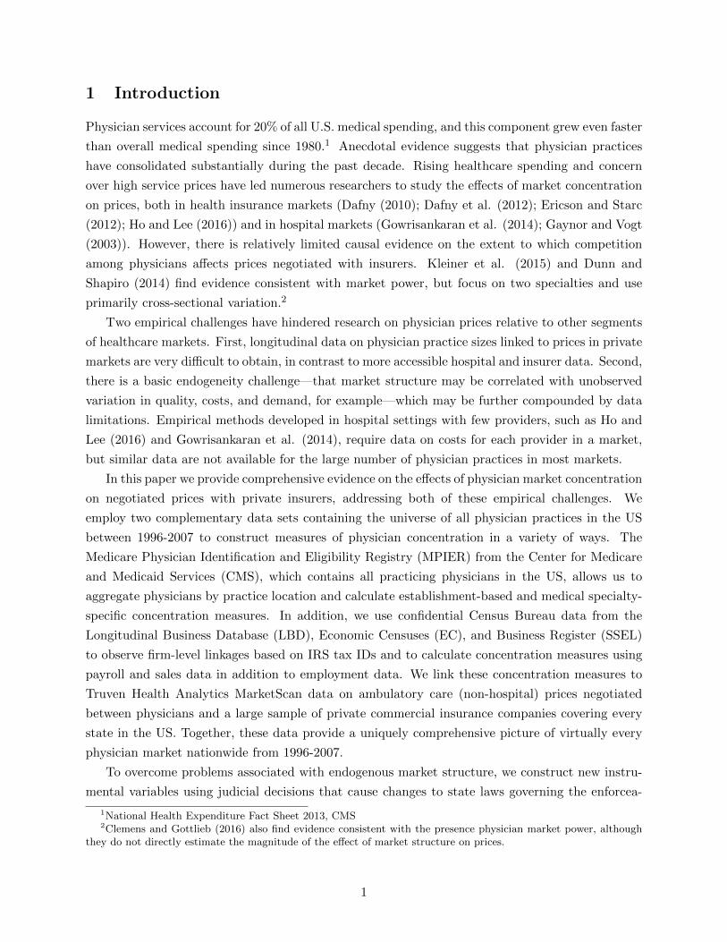
Figure 4 shows an event study plot with the same design and controls as in Figure 3, except
the dependent variable is the average physician-practice separation rate before and after a law
change. The event year dummies are scaled so that the graph can be interpreted as an increase
in the separation rate when NCA enforceability declines. The coefficient estimates suggest that an
average law change that decreases NCA enforceability is associated with a 15 percentage point jump
in the rate of job separations in the year of the law change. There is again no clear anticipatory
trend prior to the law change.
Figure 4 also shows that the average separation rate returns to the pre-event range. One might
wonder why the spike in separation rates is temporary rather than persistent. This pattern is con-
19
Figure 4: Event Study: Physician-Establishment Separation RatesBefore and After Decrease in Enforceability
-.3
-.2
-.1
0.1
.2.3
Est
ablis
hmen
t Sep
arat
ion
Rat
e
-3 -2 -1 0 1 2 3Years from Law Change
Notes: Sample includes treatment states with only one law change within the event window, and control states inthe same Census division as the treatment state that had no law changes during the corresponding event window.Estimates are from fixed effects regressions including county effects, census division by year effects, and specialtyeffects. Specialties included in sample are primary care and non-surgical specialists. Dashed lines represent 95%confidence intervals based on standard errors clustered by state-year. Year 0 is the calendar year during which thelaw change occurred, and the dependent variable is normalized to zero in year -1.
sistent with the presence of an accumulated stock of physicians who would like to switch practices
but are prevented from doing so by an NCA. When the enforceability of the NCA restriction decli-
nes, it becomes easier or less costly to move, and a large stock of physicians moves simultaneously.
Once the moves are completed there is less pent-up desire to switch practices, and separation rates
subsequently decline.
The pattern in Figure 4 bolsters the evidence that NCA laws constrain physicians’ choices over
practices, suggesting that there are organizational effects that could lead to changes in market con-
centration. Still, it is not obvious that even an exogenous event causing separations should change
establishment sizes or HHIs. Separating physicians could start new small practices, reducing the
average practice size, or join larger established practices, increasing establishment sizes. Alterna-
tively, if separations are driven by idiosyncratic preferences, a spike in separations could simply
lead to some physicians exiting a practice and other physicians entering it, with no net effect on
concentration. The large spike in separations corresponding to the timing of law changes is only
suggestive of an underlying mechanism that has the potential to cause the distribution of practice
sizes to change.
Table 2 presents fixed effects estimates of the impact of each legal index on the rate of physician
establishment births and deaths following changes in NCA laws. In each model the dependent
variable is either the number of establishments births or the number of establishment deaths, and
the independent variables are one-year lags of each legal index, county-specialty effects, and census-
20

Table 2: Fixed Effects Models of Establishment Births and Deaths
Dependent Variable: Births DeathsBy
CombinedBy
CombinedComponent Component
(1) (2) (3) (4)
Statutory Indext−1 –1.281* –0.612* –1.348* –0.734*(0.091) (0.092) (0.121) (0.124)
Protectible Interest Indext−1 0.583* 1.259* 0.609* 1.203*(0.066) (0.158) (0.089) (0.177)
Burden of Proof Indext−1 –0.633* –3.684* –0.532* –3.659*(0.117) (0.270) (0.136) (0.329)
Consideration Index Inceptiont−1 0.024 3.389* –0.354* 2.039*(0.088) (0.299) (0.090) (0.265)
Consideration Index Post-Inceptiont−1 –0.293* –0.847* 0.081* –0.458*(0.050) (0.093) (0.038) (0.074)
Blue Pencil Indext−1 0.235* 0.288* –0.197* –0.307*(0.041) (0.060) (0.048) (0.065)
Employer Termination Indext−1 –4.015* –4.673* –4.428* –4.533*(0.513) (0.630) (0.682) (0.780)
N 599,975 599,975R-Sq 0.44 0.34
Notes: Columns 1 and 3 report estimates from separate regressions on each law component, and columns 2 and 4report estimates from regressions including all 7 components. Dependent variables are the number of establishmentbirths (columns 1 and 2) and deaths (columns 3 and 4) from the MPIER data. All specifications control for theaggregate supply of physicians and include fixed effects for county by medical specialty, and census division by year.Huber-White standard errors reported in parentheses. * indicates significance at the 0.05 level.
division-year effects. Column 1 presents estimates from 7 separate regressions, each including one
legal index at a time. The coefficients suggest that six of the seven instruments have statistically
significant effects on the number of new practices born, ranging from a reduction in the birth rate of
4.0 practices per county-specialty-year per one-unit change in the Employer Termination Index, to
a 0.6 practice increase per unit increase in the Protectible Interest Index. Since a one unit change
in the legal indices is equivalent to switching between the two most extreme observed legal policies,
another way of expressing the effects is to scale by the standard deviation of each index, which
is given in Appendix Table A3. For example, a one standard deviation increase in the Employer
Termination Index is associated with 1.2 fewer practices born in a county. Four of the indices are
strongly negatively associated with practice births, suggesting that as increases in enforceability
decrease HHIs, this effect is not primarily driven by the creation of new smaller practices. Column
2 shows estimates from a model that includes all 7 indices at once. The signs of all 7 coefficients
remain the same as in column 1, and all 7 coefficients are statistically significant.
Columns 3 and 4 show similar estimates from regressions with practice deaths as the dependent
variable. Again, all seven law indices have significant effects on practice deaths, and the similar
coefficient signs across columns suggests that practice births may tend on average to accompany
practice deaths.
Finally, Table 3 shows that these changes in separation rates and establishment births and
21

Table 3: Fixed Effects Models of Establishment Sizes
Dependent Variable: Log FTE Physicians per EstablishmentBy
CombinedComponent
(1) (2)
Statutory Indext−1 –0.169* –0.140*(0.038) (0.048)
Protectible Interest Indext−1 –0.026 –0.178*(0.044) (0.070)
Burden of Proof Indext−1 –0.048 –0.262(0.042) (0.146)
Consideration Index Inceptiont−1 –0.121* 0.081(0.035) (0.162)
Consideration Index Post-Inceptiont−1 0.044 0.099*(0.031) (0.032)
Blue Pencil Indext−1 –0.151* –0.163*(0.027) (0.030)
Employer Termination Indext−1 –0.159 –0.103(0.110) (0.129)
N 379,370 379,370R-Sq 0.23
Notes: Column 1 reports estimates from separate regressions on each law component, and column 2 reports estimatesfrom a regression including all 7 components. Dependent variable is the log number of FTE physicians per esta-blishment in a county-year. All specifications include controls for the aggregate supply of physicians in the countyand fixed effects for county and census division by year. FTE establishment sizes are estimated by assigning equalpartial shares (summing to one) to all establishments at which a physician is active. All standard errors are clusteredby state-year. * indicates significance at the 0.05 level.
deaths also lead to changes in the average sizes of establishments. The dependent variable is the
log of the number of full-time equivalent physicians per establishment, where full-time equivalence
is calculated by assigning equal fractions of each physician to every establishment location at which
they treat patients at a given point in time. The independent variables include one-year lags of
each legal dimension, as well as fixed county effects and census-division-by-year effects. Since many
practices contain multiple physicians with different specialties, we do not condition on specialty
in these specifications. Column 1 shows that 6 of the 7 indices are negatively correlated with
establishment sizes when included separately, consistent with the patterns from the event studies in
Figure 3, and three of these 6 indices have significant coefficients. The significant coefficients range
from a reduction in establishment sizes of 12.1% to a reduction of 16.9% per unit change in each
index, or about –3.6% to –5.1% per standard deviation change in each index. Column 2 presents
estimates from a single regression on all 7 coefficients, which differs somewhat because a single
judicial decision can cause correlated changes in multiple indices at the same time. Nonetheless,
the evidence is generally consistent with the negative relationship between NCA enforceability and
practice sizes.
This combined evidence connects the effects of the instruments from the individual employment
22

level and physician-practice separation rates, to practice-level effects on establishment sizes, births,
and deaths, documenting the underlying steps that lead to changes in HHIs. Consistent with the
patterns from the event studies, changes in job separation rates lead to negative correlations with
new practice creation, average establishment sizes, and HHIs.
5.3 IV Assumptions
At the physician level, a change in law that alters NCA enforceability can have two effects on
practices. First, changing the ease with which an NCA can be enforced can alter the fraction
of physicians with NCAs in their contracts, changing the probability of treatment. And second,
allowing stricter NCAs to be enforced can impact the effect of treatment on the the subset of
physicians that have signed NCAs. In that sense the treatment that we use, changes in NCA laws,
measures a combined impact of the law change on selection into using an NCA and the effect of
the law change on those that use NCAs.
Causal inference of a local average treatment effect (LATE) in IV models requires the existence
of instruments with sufficient power in predicting the endogenous regressor. In addition to the
discussion of mechanisms above, we show in Section 7.1 that our instruments exceed typical power
thresholds.
The exclusion restriction necessary for the validity of the IVs holds as long as NCA law changes
affect physician service prices only through physician market concentration. In other words, changes
in NCA laws must not be correlated with the error term in the second stage equation. In our
structural equation, described below, negotiated prices depend on market concentration and fixed
specialty effects, county effects, medical facility type effects, procedure effects, and census-division-
by-year effects. By conditioning on this set of covariates, law changes can only be potentially
correlated with the structural error if NCA laws affect negotiated prices across practices within
a given market, defined by geography and medical specialty, and through some mechanism other
than market concentration.
Although exclusion restrictions are not formally testable, Lavetti et al. (2016) provide direct
evidence that is useful for evaluating the plausibility of this condition. Using survey data from
about 2,000 physicians with information on whether each physician has signed an NCA linked to
negotiated prices with private insurers at the practice level, they find that the use of NCAs has
precisely no effect on negotiated prices conditional on fixed market effects and practice size. They
find that, within a given geographic market, the standard deviation in negotiated prices across
practices for a given procedure is about 39% of the mean price, but the average price difference
associated with NCA use is only 2% of the mean negotiated price and is not statistically significant.
In addition, the price difference between NCA users and non-users is no different in higher versus
lower NCA enforcement states. To the extent that NCAs affect prices, this evidence suggests
that it occurs either across markets or through practice size and concentration measures, which is
consistent with the requirements of the exclusion restriction.
A second related concern with the exclusion restriction is that there could be a correlation
23

between physician quality and the use of NCAs. For example, it is conceptually possible that there
is selection on physician quality into practices that require NCAs. The survey data used in Lavetti
et al. (2016) are again useful for demonstrating that there is no evidence of quality differences
associated with the use of NCAs. This conclusion comes from three sources of information. First,
to the extent that physician quality is correlated with prices, a quality difference would be reflected
in a price difference between NCA users and non NCA users in the same market, but such a price
difference does not exist. Second, there is no difference in the amount of prior experience physicians
have when entering practices that use NCAs versus those that don’t. Physician experience is
strongly correlated with measures of patient satisfaction and perceived quality (Choudhry et al.,
2005.) Finally, the survey data contain rich information about quality from a section of vignette-
based questions that were designed by clinical experts to directly elicit knowledge about clinical
best practices, guidelines, diagnostic skill, and appropriate treatment recommendations. The study
finds no differences associated with the use of NCAs in either the distributions of responses to
questions or in aggregate measures of compliance with guidelines.
A closer examination of the data also supports the exogeneity of judicial changes on NCA laws,
which is required to satisfy the assumption of random assignment. In addition to showing an
absence of pre-trends in the event studies, which supports the notion that judicial decisions were
not made in response to trends in physician concentration or prices, it is also informative to analyze
the law changes directly. Since judicial decisions are accompanied by opinions written by judges
that describe the rationales that led them to their decisions, we can identify the judicial decisions
used in our data that were related to physicians and verify that our findings are not sensitive to
excluding these events. We further examine law changes to verify that they were not systematically
related to other state-level political and economic factors that could also affect prices. This evidence
is discussed in Section 7.4.
The final IV assumption is monotonicity. Note that the monotonicity condition in the case of our
instruments is not that all seven instruments should move the HHI in the same direction. Rather,
the condition requires that each law dimension moves HHIs in all states in the same direction. In
split-sample analyses of high and low enforcement states, or states with positive or negative law
changes, we find suggestive evidence that is generally consistent with this assumption. Under these
IV assumptions, each instrument identifies a separate LATE, and our second-stage estimand is an
average of these LATEs. As we will show, the seven LATEs are all similar to each other, so the
average is informative.
6 Empirical Model
We use two-stage least squares to estimate the effects of changes in state NCA laws on physician
market concentration. Since physician practice sizes could be influenced by many factors, inclu-
ding insurer market concentration, consumer demand, and the dynamics of medical markets, we
estimate fixed effects specifications that control for as much of this unobserved heterogeneity as
possible. To differentiate the effects of increases in HHI driven by larger firms as opposed to larger
24
establishments, our main estimates from the Census LBD include both endogenous regressors in
the same specification. This gives two first-stage equations:
ECmc(t−1) = α1 + β1NCA′c(t−1,t−2) + β2Ins HHIc(t−1) + ηm + πf + θp + γc + νdt + εmc(t−1)
FCc(t−1) = α2 + β3NCA′c(t−1,t−2) + β4Ins HHIc(t−1) + ηm + πf + θp + γc + νdt + εmc(t−1)
and the second-stage equation is:
Pmfpct = α3 + β5ECmc(t−1) + β6FCc(t−1) + β7Ins HHIc(t−1) + ηm + πf
+ θp + γc + νdt + εmfpct (5)
where m denotes medical specialty, c county, f facility type, p procedure code, d census division,
and t year. NCA′ct is a vector of the seven law instruments, measured at the state-year level.
ECmct is the establishment-based measure of market concentration, in contrast to FCct, the firm-
based concentration measure. Ins HHIc(t−1) is the HHI of health insurance firms in the state,
calculated using the Census LBD. ηm, πf , θp, γc, and νdt are fixed effects for specialties, facility
types, procedure codes, county, and census division-by-year effects, respectively. Our main specifi-
cations use HHIs as concentration measures, though we also show that our findings are robust to a
range of alternative concentration measures, including average practice size, the negative log HHI
transformation, and the four and eight-firm concentration ratios.
By including census-division by year effects, the estimates identify the extent to which concen-
tration and prices move differentially in markets within a state that experiences a change in NCA
laws relative to markets in the other, on average, 4.6 neighboring states in the same census division.
This allows each census division to have any arbitrary unobserved idiosyncratic variation over time
in both concentration and prices, which we use in lieu of imposing functional form restrictions on
time trends.
Since negotiations between physicians and insurers tend to occur annually (or less frequently,)
we use a lagged specification that allows average transaction prices observed in year t to be affected
by concentration in year t− 1. This lagged specification is also used in Dafny et al. (2012), Dunn
and Shapiro (2014), and Baker et al. (2014). Moreover, since there may be a lag in physicians
responding to NCA law changes, the first stage assumes that concentration effects occur either
in the contemporaneous or lagged year. Since the dependent variable in the first stage is already
lagged, this implies the instruments include first and second lags of the legal indices.
Although our main results are based on the above specification, we also estimate a variety
of robustness models using only MPIER data, since Census Bureau confidentiality restrictions
make it prohibitive to disclose results from a large number of alternative specifications. In these
specifications there is a single first-stage equation corresponding to ECmct, and the models exclude
FCc(t−1) and Ins HHIc(t−1). Using the MPIER we assess sensitivity to market definitions, different
alternative assumptions about the treatment of multi-specialty practices in calculating HHIs, with
alternative measures of market concentration and firm sizes, dropping outlier law changes, using
25

only the subset of instruments with negative first stage coefficients, and controlling for insurance
market HHI. Rather than focusing entirely on counties as market definitions, we also estimate the
model using Primary Care Service Areas (PCSA) and Hospital Service Areas (HSA). PCSA and
HSA definitions come from the Dartmouth Atlas of Healthcare, and are calculated by analyzing
patients’ travel patterns to providers to primary care physicians and hospitals, respectively. PCSAs
are on average smaller than counties (there are 6,542 defined PCSAs, or about 2.1 PCSAs per
county) and HSAs are roughly similar in size to counties on average, but are defined based on
where patients travel for hospital services. Since patients tend to travel short distances for primary
care and longer distances for non-emergency hospital care, we view these two measures as plausible
lower and upper bounds on the relevant market for physicians, on average.
7 Results
7.1 First-Stage Effects of NCA Laws on HHI
Regression results corroborate the evidence from Section 5 that increases in NCA enforceability
have strong, and generally negative, effects on physician market concentration. Table 4 presents
estimates from the first-stage models based on employment. The first column shows estimates from
seven separate regressions of the establishment-level HHI on each of the seven legal indices. Five of
the seven legal indices are statistically significant, and six of the seven have negative coefficients.
The dependent variable, HHI, is scaled to range from 0 to 100, so the coefficient on the Burden
of Proof Index, for example, suggests that a one unit increase in the index decreases the HHI by
452 points on a 10,000 point scale. Scaling by the standard deviation of the Burden of Proof Index
(0.27) implies that a one standard deviation increase reduces the HHI by about 122 points.
Column 2 presents estimates from a similar specification that includes all 7 seven instruments.
The Angrist-Pischke excluded instrument F-statistic is 87, and four of the instruments are statisti-
cally significant at the 0.01 level in this model. By comparison, the Stock and Yogo (1997) critical
F-statistics thresholds range from about 9 to 12 for achieving 10% relative bias under 2SLS with
one endogenous regressor and 3 to 14 instruments. The full table of first-stage results showing
both first and second lags of all 7 instruments is shown in the appendix (Table A4). When the
second lags of each index are used as instruments, the F-statistic is similar (110.45), and when
both first and second lags are used the F-statistic is 460, suggesting that any of these choices of
lag specifications has sufficient power. In all three specifications, the fixed effects and excluded
instruments explain about 75% of the variation in county-specialty-year HHIs.
The main results using Census data are presented in columns 3 and 4, which correspond to
the two jointly-estimated first-stage equations from Section 6. Column 3 shows estimates from the
establishment HHI first stage, and column 4 from the firm HHI equation. There are three main
points to note about these estimates. First, regarding instrument power, the main limitation of the
models estimated using Census data relative to the MPIER estimates is that specialties are not
observed, which substantially weakens the first-stage power. However, the F-statistics still suggest
26
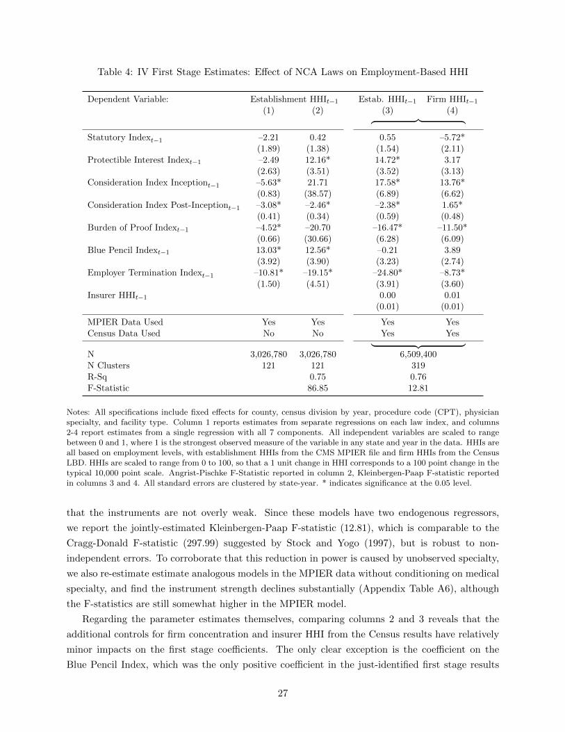
Table 4: IV First Stage Estimates: Effect of NCA Laws on Employment-Based HHI
Dependent Variable: Establishment HHIt−1 Estab. HHIt−1 Firm HHIt−1
(1) (2) (3) (4)︷ ︸︸ ︷Statutory Indext−1 –2.21 0.42 0.55 –5.72*
(1.89) (1.38) (1.54) (2.11)Protectible Interest Indext−1 –2.49 12.16* 14.72* 3.17
(2.63) (3.51) (3.52) (3.13)Consideration Index Inceptiont−1 –5.63* 21.71 17.58* 13.76*
(0.83) (38.57) (6.89) (6.62)Consideration Index Post-Inceptiont−1 –3.08* –2.46* –2.38* 1.65*
(0.41) (0.34) (0.59) (0.48)Burden of Proof Indext−1 –4.52* –20.70 –16.47* –11.50*
(0.66) (30.66) (6.28) (6.09)Blue Pencil Indext−1 13.03* 12.56* –0.21 3.89
(3.92) (3.90) (3.23) (2.74)Employer Termination Indext−1 –10.81* –19.15* –24.80* –8.73*
(1.50) (4.51) (3.91) (3.60)Insurer HHIt−1 0.00 0.01
(0.01) (0.01)
MPIER Data Used Yes Yes Yes YesCensus Data Used No No Yes Yes︸ ︷︷ ︸N 3,026,780 3,026,780 6,509,400N Clusters 121 121 319R-Sq 0.75 0.76F-Statistic 86.85 12.81
Notes: All specifications include fixed effects for county, census division by year, procedure code (CPT), physicianspecialty, and facility type. Column 1 reports estimates from separate regressions on each law index, and columns2-4 report estimates from a single regression with all 7 components. All independent variables are scaled to rangebetween 0 and 1, where 1 is the strongest observed measure of the variable in any state and year in the data. HHIs areall based on employment levels, with establishment HHIs from the CMS MPIER file and firm HHIs from the CensusLBD. HHIs are scaled to range from 0 to 100, so that a 1 unit change in HHI corresponds to a 100 point change in thetypical 10,000 point scale. Angrist-Pischke F-Statistic reported in column 2, Kleinbergen-Paap F-statistic reportedin columns 3 and 4. All standard errors are clustered by state-year. * indicates significance at the 0.05 level.
that the instruments are not overly weak. Since these models have two endogenous regressors,
we report the jointly-estimated Kleinbergen-Paap F-statistic (12.81), which is comparable to the
Cragg-Donald F-statistic (297.99) suggested by Stock and Yogo (1997), but is robust to non-
independent errors. To corroborate that this reduction in power is caused by unobserved specialty,
we also re-estimate estimate analogous models in the MPIER data without conditioning on medical
specialty, and find the instrument strength declines substantially (Appendix Table A6), although
the F-statistics are still somewhat higher in the MPIER model.
Regarding the parameter estimates themselves, comparing columns 2 and 3 reveals that the
additional controls for firm concentration and insurer HHI from the Census results have relatively
minor impacts on the first stage coefficients. The only clear exception is the coefficient on the
Blue Pencil Index, which was the only positive coefficient in the just-identified first stage results
27

but is insignificant and negative once the additional Census controls are introduced. Finally, it is
notable that the legal indices have different effects on the establishment and firm HHI measures,
as can be seen by comparing column 3 to column 4. For example, an increase in the Statutory
Index has a negative effect on firm HHIs of –5.7 but no effect on establishment HHIs. In contrast,
the Protectible Interest Index has a significant positive effect on establishment HHIs of about 17.6
but very modest effects on firm HHIs. This pattern suggests the presence of heterogeneity in the
features of the legal indices that affect firm organizational incentives, with some laws having more
impact on multi-establishment firm incentives and while others appear to impact the sizes of each
establishment.
Table 5: IV First Stage Estimates: Effect of NCA Laws on Sales-Based HHI
Dependent Variable: Estab. HHIt−1 Firm HHIt−1
(1) (2)︷ ︸︸ ︷Statutory Indext−1 –0.25 –3.09
(1.48) (2.33)Protectible Interest Indext−1 14.11* 7.23*
(3.36) (3.56)Consideration Index Inceptiont−1 17.26* 22.56
(6.94) (13.17)Consideration Index Post-Inceptiont−1 –2.18* 2.79*
(0.59) (1.01)Burden of Proof Indext−1 –16.15* –19.49
(6.33) (12.31)Blue Pencil Indext−1 –0.15 0.53
(3.13) (3.49)Employer Termination Indext−1 –24.06* –10.28*
(3.77) (4.31)Insurer HHIt−1 0.00 –0.04
(0.01) (0.02)
MPIER Data Used Yes YesCensus Data Used Yes Yes︸ ︷︷ ︸N 6,329,900N Clusters 319R-Sq 0.83F-Statistic 13.56
Notes: All specifications include fixed effects for county, census division by year, procedure code (CPT), physicianspecialty, and facility type. Legal indices are scaled to range between 0 and 1, where 1 is the strongest observedmeasure of the variable in any state and year in the data. Firm HHIs are based on sales from the Census LBD andSSEL, and establishment HHIs are based on employment levels from MPIER. HHIs are scaled to range from 0 to100, so that a 1 unit change in HHI corresponds to a 100 point change in the typical 10,000 point scale. All standarderrors are clustered by state-year. Kleinbergen-Paap F-statistic reported. * indicates significance at the 0.05 level.
Table 5 presents first-stage estimates using HHIs based on sales data from the Census LBD,
Economic Census, and SSEL, instead of on employment. There are two main conclusions from
these results. First, all seven of the coefficients in column 2 have the same sign as the coefficients
28
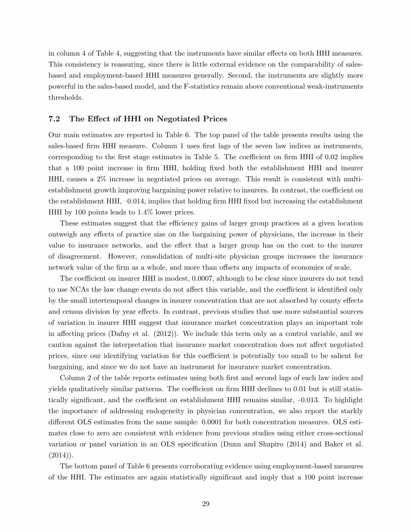
in column 4 of Table 4, suggesting that the instruments have similar effects on both HHI measures.
This consistency is reassuring, since there is little external evidence on the comparability of sales-
based and employment-based HHI measures generally. Second, the instruments are slightly more
powerful in the sales-based model, and the F-statistics remain above conventional weak-instruments
thresholds.
7.2 The Effect of HHI on Negotiated Prices
Our main estimates are reported in Table 6. The top panel of the table presents results using the
sales-based firm HHI measure. Column 1 uses first lags of the seven law indices as instruments,
corresponding to the first stage estimates in Table 5. The coefficient on firm HHI of 0.02 implies
that a 100 point increase in firm HHI, holding fixed both the establishment HHI and insurer
HHI, causes a 2% increase in negotiated prices on average. This result is consistent with multi-
establishment growth improving bargaining power relative to insurers. In contrast, the coefficient on
the establishment HHI, –0.014, implies that holding firm HHI fixed but increasing the establishment
HHI by 100 points leads to 1.4% lower prices.
These estimates suggest that the efficiency gains of larger group practices at a given location
outweigh any effects of practice size on the bargaining power of physicians, the increase in their
value to insurance networks, and the effect that a larger group has on the cost to the insurer
of disagreement. However, consolidation of multi-site physician groups increases the insurance
network value of the firm as a whole, and more than offsets any impacts of economies of scale.
The coefficient on insurer HHI is modest, 0.0007, although to be clear since insurers do not tend
to use NCAs the law change events do not affect this variable, and the coefficient is identified only
by the small intertemporal changes in insurer concentration that are not absorbed by county effects
and census division by year effects. In contrast, previous studies that use more substantial sources
of variation in insurer HHI suggest that insurance market concentration plays an important role
in affecting prices (Dafny et al. (2012)). We include this term only as a control variable, and we
caution against the interpretation that insurance market concentration does not affect negotiated
prices, since our identifying variation for this coefficient is potentially too small to be salient for
bargaining, and since we do not have an instrument for insurance market concentration.
Column 2 of the table reports estimates using both first and second lags of each law index and
yields qualitatively similar patterns. The coefficient on firm HHI declines to 0.01 but is still statis-
tically significant, and the coefficient on establishment HHI remains similar, –0.013. To highlight
the importance of addressing endogeneity in physician concentration, we also report the starkly
different OLS estimates from the same sample: 0.0001 for both concentration measures. OLS esti-
mates close to zero are consistent with evidence from previous studies using either cross-sectional
variation or panel variation in an OLS specification (Dunn and Shapiro (2014) and Baker et al.
(2014)).
The bottom panel of Table 6 presents corroborating evidence using employment-based measures
of the HHI. The estimates are again statistically significant and imply that a 100 point increase
29

Table 6: Main Estimates: Effect of Market Concentration on Negotiated Prices
Dependent Variable: ln(Price)IV IV
OLSFirst BothLags Lags(1) (2) (3)
Physician Firm HHI, Sales-Based 0.020* 0.010* 0.0001*(0.009) (0.004) (0.0000)
Physician Establishment HHI –0.014* –0.013* 0.0001*(0.006) (0.005) (0.0000)
Insurer HHI 0.0007 0.0003 –0.0001(0.0006) (0.0004) (0.0003)
N 6,329,900 6,329,900 6,329,900N Clusters 319 319 319F-Stat (Cragg-Donald) 270.27 143.79F-Stat (Kleinbergen-Paap) 13.56 10.32
Physician Firm HHI, Employment-Based 0.016* 0.010* 0.0001*(0.007) (0.005) (0.0000)
Physician Establishment HHI –0.014* –0.017* 0.0001*(0.005) (0.005) (0.0000)
Insurer HHI 0.0000 0.0000 0.0000(0.0002) (0.0002) (0.0003)
N 6,509,400 6,509,400 6,509,400N Clusters 319 319 319F-Stat (Cragg-Donald) 297.99 174.35F-Stat (Kleinbergen-Paap) 12.81 10.44
Notes: All specifications include fixed effects for county, census division by year, procedure code (CPT), physicianspecialty, and facility type. Data for physician firm and insurer HHIs in these regressions come from the Census’ LBD(employment) and SSEL (sales). Physician establishment HHIs are from MPIER. HHIs are scaled to range from 0to 100, so that a 1 unit change in HHI corresponds to a 100 point change in the typical 10,000 point scale. InsurerHHIs are calculated from firm-level in-state sales. Medical specialties are observed in price data but not in Censusdata used to calculate physician HHIs. All standard errors are clustered by state-year. * indicates significance at the0.05 level.
in firm HHI, conditional on establishment and insurer HHI, increase negotiated prices by about
1% to 1.6%, while the same size increase in establishment HHI decreases prices by 1.4% to 1.7%.
These estimates are consistent with the evidence from the first stage models that the sales-based
and employment-based HHI measures yield similar results.
By comparison, Table 7 presents IV estimates using only the MPIER data, where firm HHI is
not observable. The results suggest that a 100 point increase in the establishment HHI leads to a
2.4% to 2.8% reduction in average negotiated prices, somewhat larger than in the estimates with
Census data that control for firm and insurer HHI. The estimated effect is on the upper end of this
range when first lags are used as instruments and on the lower end when second lags are used.
Since the majority of our robustness analyses can only be conducted using MPIER data, we
first seek to understand why the MPIER estimates differ somewhat from the Census estimates. To
30

Table 7: OLS and IV Second Stage: Effect of Establishment-Based Market Concentration onPrices
Dependent Variable: ln(Price)tIV IV IV OLS(1) (2) (3) (4)
HHIt−1 –0.0283* –0.0235* –0.0251* 0.0002*(0.0056) (0.0045) (0.0047) (0.0000)
Instruments First Lags Second Lags Both Lags
N 3,026,780 3,026,780 3,026,780 3,026,780N Clusters 121 121 121 121R-Sq 0.97 0.98 0.98 0.821st Stage F-Stat 86.85 110.45 460.22
Notes: All specifications include fixed effects for county, census division by year, procedure code (CPT), physicianspecialty, and facility type. HHI is calculated from establishment sizes in MPIER data, provided by CMS. HHI isscaled to range from 0 to 100, so that a 1 unit change in HHI corresponds to a 100 point change in the typical10,000 point scale. All standard errors are clustered by state-year. Angrist-Pischke F-Statistic reported. * indicatessignificance at the 0.05 level.
that end, we collapse the MPIER HHI measures as though physician specialties were unobserved,
and we re-estimate the IV models. The results, shown in Appendix Table A6, suggest that the
effect of establishment HHI is between –0.011 and –0.015 in all specifications, very similar to Census
estimates when the data structure is made more comparable. We also estimate our main MPIER
HHI specifications including the Census insurer HHI control but no firm HHI, and we find that it
does not substantively alter those estimates either. These results provide some reassurance that
the robustness analyses using MPIER data are relevant to our main Census estimates.
Returning to the discussion of the exclusion restriction from Section 5.3, one additional form of
evidence in support of this restriction comes from the consistency of estimates when we estimate
the IV model using only one legal index at a time, shown in Table 8. Column 1 of the table presents
second-stage estimates from 7 separate just-identified IV regressions using only the first-lags of each
instrument, one at a time, and column 2 presents estimates using first and second lags of each index.
All 14 models yield negative coefficients on the establishment HHI, and 10 of the 14 estimates are
statistically significant.
This result is reassuring because if the exclusion restriction were violated due to a direct effect
of the instruments on practice cost functions, the differences in the legal nature of the instruments
would presumably cause heterogeneity by instrument in the second-stage estimates. For example,
whereas the Consideration Index affects the way employment contracts are written by affecting
whether compensation for NCAs must be explicit, it is far less obvious that law dimensions such as
the Burden of Proof Index or the Blue Pencil Index could potentially impact practice cost functions.
Both of these dimensions relate to the specific procedures used during litigation related to NCA
contracts and are only relevant when an employment spell is terminated and an NCA clause is
31

Table 8: IV Results Estimated Separately by Law Component
Dependent Variable: ln(Price)
Instruments:First BothLags Lags
Statutory Index –0.047 –0.029*(0.061) (0.015)[1.37] [3.58]
Protectible Interest Index –0.003 –0.019(0.051) (0.011)[0.90] [3.65]
Consideration Index Inception –0.043* –0.032*(0.011) (0.007)[45.68] [246.67]
Consideration Index Post-Inception –0.020* –0.021*(0.009) (0.008)[55.70] [33.66]
Burden of Proof Index –0.043* –0.031*(0.011) (0.006)[46.98] [260.14]
Blue Pencil Index –0.007 –0.008*(0.005) (0.003)[11.05] [24.31]
Employer Termination Index –0.024* –0.024*(0.006) (0.006)[52.04] [26.08]
Notes: Each cell shows the second stage IV estimate of the effect of lagged HHI on log prices using a single legalcomponent as the instrument. The first column displays just-identified models using the first lag of each index.The second column includes both the first and second lags of the legal component as instruments. All specificationsinclude fixed effects for county, census division by year, procedure code (CPT), physician specialty, and facility type.HHI is calculated from establishment sizes in MPIER data, provided by CMS. HHI is scaled to range from 0 to 100,so that a 1 unit change in HHI corresponds to a 100 point change in the typical 10,000 point scale. All standarderrors, in parentheses, are clustered by state-year. First-stage Angrist-Pischke F-statistics are shown in brackets. *indicates significance at the 0.05 level.
litigated. In order for the Burden of Proof index to violate the exclusion restriction, it would
have to be the case that for an employment contract that was previously agreed to by both the
worker and firm, after being potentially violated and litigated, the cost to the firm of producing
evidence for the litigation affected prices negotiated with insurers. Similarly, with respect to the
Blue Pencil Index, it would have to be true that negotiated prices would be affected by a change
in the ability of a judge to ex post adjust the terms of a contract that was operable during the
time of employment. The consistency of estimates over a range of instruments, each of which has
unique and distinct legal mechanisms for affecting organizational incentives, makes it less likely
that a potential violation of the exclusion restriction for any one legal measure could be driving
the overall pattern of results.
Taken together, our results from MPIER and Census data suggest that the effects of conso-
lidation on prices depend on a tradeoff between the efficiency gains of larger establishments and
32

the increased negotiating power associated with bargaining as a larger organization. Larger esta-
blishments allow efficiency gains via economies of scale that dominate leverage effects from size
in negotiation, causing negotiated prices to fall. These economies of scale can arise, for example,
when physician practices share equipment, information systems, laboratory facilities, nurses, and
technical and administrative staff over a larger number of physicians and patients. The contrasting
firm-level estimates, however, suggest that consolidation of multi-establishment firms increases the
combined impact of bargaining power and the value of a larger physician practice to an insurer
network by more than any efficiency gains within the practice, leading to higher negotiated prices.
This result is consistent with the notion that most of the efficiency gains from larger physician firms
come from increases in practice size at a given location; meanwhile, consolidation across locations
has smaller efficiency gains but still affects bargaining leverage in negotiation, causing a net positive
effect on prices.
7.3 Reduced-Form Price Effects
Figure 5 presents event studies of the reduced-form effects of NCA law changes on negotiated
prices. Each of the four figures suggests the same two conclusions: increasing NCA enforceability
leads to higher prices, and states that experienced law changes show little evidence of differential
price trends prior to the law changes. In addition, the price effects appear to flatten after about
two years, suggesting that the law changes primarily impact price levels as opposed to rates of
growth, and the effects occur fairly quickly. The figures are constructed similarly to the previous
event studies in Figure 3, comparing treatment states with exactly one law change within the event
window to control states in the same census division with no law changes. The plotted coefficients
are from regressions of procedure-level log prices on event year indicators and the same control
variables used in the regressions: county effects, census division by year effects, specialty effects,
facility type effects, and procedure code effects.
The combination of these reduced-form event studies and our main results provides policy-
relevant information. In our main regression results the net direction of aggregate price effects
is ambiguous—it depends on whether law changes tend to cause more within-establishment or
across-establishment growth. This ambiguity is difficult to reconcile directly since the LBD does
not include specialty information, preventing an accurate decomposition of the components of
variation in concentration. The reduced-form effects are consistent with the predominant impacts
of NCA law changes occurring through within-establishment growth.
Figure 5b scales the event year indicators by the size of the law change, so that the estimates
can be interpreted as the impact of a 0.1 unit increase in the average NCA enforceability index. The
figure shows that the magnitudes of the price effects are larger when the size of the law changes are
larger, and a 0.1 unit increase in NCA enforceability leads to about 9.8% higher prices on average
within 2 years. Given the size of the market for physician services, about $635 billion in 2015, these
estimates suggest that the impact of NCA enforcement policies on physician prices are of first-order
importance.
33

Figure 5: Event Study Plots: Reduced-Form Price Effects
Row
1:A
llL
awC
han
ges
Column 1: Binary Indicator
for Increase in NCA Index
(a)
Column 2: Weighted by Size
of NCA Index Increase
(b)
Row
2:N
egat
ive
Var
iati
onO
nly
(c) (d)
Notes: Sample includes treatment states with only one law change within the event window, and control states inthe same Census division as the treatment state that had no law changes during the corresponding event window.Estimates are from fixed effects regressions including county effects, census division by year effects, procedure codeeffects, facility type effects, and specialty effects. Specialties included in sample are primary care and non-surgicalspecialists. Dashed lines represent 95% confidence intervals based on standard errors clustered by state-year. Year 0is the calendar year during which the law change occurred, and the dependent variable is normalized to zero in year-1.
Figures 5c and 5d are estimated using only variation that decreases NCA enforceability, although
the coefficients are scaled by -1 where appropriate to conform with the interpretation of the price
effect of increasing enforceability. These figures show that decreases in enforceability have (negative)
price effects that are slightly larger in magnitude, though the results are generally consistent with
symmetric effects.
Regression versions of the reduced-form results using the full sample, instead of the limited
event study sample that only includes the 7 treatment states with exactly 1 law change during the
event window and the corresponding control states with zero law changes, are shown in Table 9.
The results in the full sample have the same sign as the event study estimates and suggest prices
increase by 3.7% after 2 years per 0.1 unit increase in the weighted average NCA index, compared
34

Table 9: Reduced-Form Price Effects, by NCA Index
Dependent Variable: ln(Price)NCA(t−1) NCA(t−2)
NCA Index (Weighted Average) 0.491* 0.370*(0.094) (0.095)
Statutory Index 0.103 0.118*(0.062) (0.038)
Protectible Interest Index –0.007 –0.094(0.121) (0.105)
Consideration Index Inception 0.242* 0.179*(0.045) (0.049)
Consideration Index Post-Inception 0.062* 0.059*(0.030) (0.025)
Burden of Proof Index 0.193* 0.131*(0.036) (0.039)
Blue Pencil Index –0.093 –0.147*(0.078) (0.061)
Employer Termination Index 0.260* 0.177*(0.082) (0.075)
N (Each Model) 3,026,780 3,026,780
Notes: Each coefficient comes from a separate regression of log prices on either the first lag (column 1) or second lag(column 2) the corresponding legal index. Each legal index is scaled to range from 0 to 1, where 1 corresponds tothe highest observed enforceability measure for that index. All specifications include fixed effects for county, censusdivision by year, procedure code (CPT), physician specialty, and facility type. All standard errors, in parentheses,are clustered by state-year. * indicates significance at the 0.05 level.
to 9.8% in the event study sample. Rescaling the 3.7% estimate by the standard deviation of the
NCA index (0.259) suggests that a one standard deviation increase in NCA enforceability increases
average prices by 9.6%. Six of the seven instruments have significant reduced-form effects on prices,
and five have positive coefficients. The only instrument with a negative and significant sign, the
Blue Pencil Index, also happens to be the only instrument with a positive and significant sign in
the first stage regressions, which is why all 7 second-stage IV estimates have the same sign in the
just-identified models.
7.4 Heterogeneity and Robustness
In this section we provide a concise overview of many supplemental analyses conducted to assess
the robustness of our results to model assumptions and to potential data measurement concerns.
Market Structure Measure: Although our main estimates rely on HHIs, the most commonly
used measure of market concentration in the literature (Gaynor et al. (2015)), interpreting estimates
from models using HHI as estimates of the elasticity of demand requires the potentially undesirable
assumptions that goods are homogeneous and firms engage in Cournot competition (see Section 3.2).
Since we cannot estimate firm conduct directly without detailed claims data, we test the sensitivity
35

of our estimates to these assumptions by re-estimating the model using the negative log HHI
transformation, average establishment size, 4-firm market share, and 8-firm market share.
Table 10: Alternative Measures of Market Concentration (Establishment-Based)
Dependent Variable: ln(Price)tIV IV OLS
Instruments:First BothLags Lags
Negative Log HHI(t−1) 0.190* 0.283* 0.004*
(0.084) (0.092) (0.001)1st Stage F-Stat [80.33] [2043.69]
Mean Establishment Size(t−1) –0.043* –0.034* 0.0003*
(0.014) (0.013) (0.0000)1st Stage F-Stat [245.13] [652.49]
4-Firm Market Share(t−1) –0.021* –0.022* –0.0001
(0.007) (0.006) (0.0001)1st Stage F-Stat [21.96] [11.81]
8-Firm Market Share(t−1) –0.030* –0.029* –0.0001
(0.011) (0.010) (0.0001)1st Stage F-Stat [13.96] [4.95]
Notes: All specifications include fixed effects for county, census division by year, procedure code (CPT), physicianspecialty, and facility type. All concentration measures are calculated from establishment sizes in MPIER data,provided by CMS. 4-Firm and 8-Firm Market Shares are measured from 0 to 100. Angrist-Pischke F-Statisticsreported in brackets. All standard errors are clustered by state-year. * indicates significance at the 0.05 level.
Table 10 shows that the qualitative conclusions are identical for all of these choices of market
structure. In the negative log HHI specification, the sign is positive (which is consistent since the
measure is negated), and the bias relative to the OLS specification goes in the same direction.
When average establishment size is used we find that increasing the average number of physicians
in a practice by one reduces negotiated prices by about 3.4% to 4.3%. Similarly, in markets that
become more concentrated in terms of the market shares of the 4 largest or 8 largest establishments,
negotiated prices fall significantly. Across the variety of market structure measures and instrument
specifications, we conclude that there is a statistically significant negative relationship between
market concentration and negotiated prices in all fifteen models tested.
Geographic Market Definition: Although county is a commonly used market definition (See
Baker et al. (2015), Schneider et al. (2008),) we also test whether the results are sensitive to this
choice. Market definition is often a crucial assumption in evaluating policies aimed at ensuring
sufficient levels of competition, but since we rely on changes in concentration within markets,
our estimates do not appear to be very sensitive to the assumption of market definition. The
magnitudes of our estimates are very stable when using either smaller or larger market definition
assumptions. Table 11 presents estimates of the main specification using counties, hospital service
areas (HSAs), and primary care service areas (PCSAs) as potential market definitions. HSAs are
defined by the Dartmouth Atlas of Healthcare using data on patient locations and their choices
36

between hospitals. We chose HSAs as a plausible upper bound on the size of markets, since patients
tend to travel farther on average to hospitals than they do for ambulatory physician visits. PCSAs
are similarly defined by the Dartmouth Atlas but are based on choices of primary care physicians
only. Since patients tend to travel farther to visit specialists than they do to visit primary care
physicians, PCSAs are likely to be smaller on average than the appropriate overall market definition
for physicians.
Table 11: Sensitivity of MPIER IV Estimates to Market Definition
Dependent Variable: ln(Price)County HSA PCSA
Full Sample
HHI(t−1) –0.025* –0.023* –0.029*
(0.005) (0.008) (0.008)1st Stage F-Stat [460.2] [2119.6] [270.4]
Primary Care
HHI(t−1) –0.017* –0.018* –0.024*
(0.005) (0.005) (0.004)1st Stage F-Stat [542.3] [63.1] [122.2]
Notes: All specifications include fixed effects for the corresponding geographic market, census division by year,procedure code (CPT), physician specialty, and facility type. HHI is calculated from establishment sizes in MPIERdata, provided by CMS. HHIs are scaled to range from 0 to 100, so that a 1 unit change in HHI corresponds to a100 point change in the typical 10,000 point scale. In each specification the instruments include all lagged and twicelagged law components, as in column (3) of Table 7. Standard errors, in parentheses, are clustered by state-year.First-stage Angrist-Pischke F-statistics are reported in square parentheses. * indicates significance at the 0.05 level.
The estimates are very similar for all three market definitions, ranging from -2.3% in HSAs to
-2.9% in PCSAs. This conclusion also holds within every physician specialty group, with significant
negative effects for every combination of market definition and specialty, and a general pattern that
effects are slightly larger in magnitude in smaller PCSA markets. Overall, we conclude that market
definition assumptions do not substantively alter our conclusions.
Sensitivity to Large NCA Law Changes: Figure A1 shows that a small number of law changes
are of much larger magnitude than the average change. Appendix Table A7 presents estimates in
which we drop outlier states with very large NCA law changes. The estimates are very similar,
remain statistically significantly different from zero, and are not significantly different from each
other. The first-stage power increases slightly in all three specifications.
Treatment of Multi-Specialty Practices: Defining markets by specialty involves assumptions
about how to treat physicians in multi-specialty practices. For example, when defining a market for
orthopedists, how should one treat practices that contain orthopedists as well as radiologists? One
approach is to ignore radiologists altogether, and only consider the market shares of orthopedists in
the geographic market. However, an insurer concerned about the negative consequences of failing
to reach an agreement with such a practice may care about the consequences of losing both the
37

orthopedists and the radiologists. Our main specifications calculate HHIs using all physicians in
any practice containing at least one physician in a given specialty. In Appendix Table A8 we
consider 4 different possible sets of assumptions about the treatment of multispecialty practices in
measuring concentration. The estimates are similar under every alternative assumption tested.
Heterogeneity by Specialty Type: As discussed in Section 2, there may be heterogeneity in
the usage and value of NCA contracts for physicians with different specialties. Since the benefits
of NCAs in protecting the value of patient stocks is likely to be largest for physicians with many
repeated interactions with the same patients, hospital-based practices that employ specialists like
surgeons may derive less value from NCAs. This notion is consistent with the findings of Lavetti,
Table 12: Effect of Concentration on Prices by Medical Specialty
Dependent Variable: ln(Price)t
InstrumentsFirst BothLags Lags(1) (2)
All Physicians
HHIt−1 –0.028* –0.025*(0.006) (0.005)
N 3,026,780 3,026,7801st Stage F-Stat 86.9 460.2
Primary Care Physicians
HHIt−1 –0.024* –0.017*(0.005) (0.005)
N 473,033 473,0331st Stage F-Stat 47.2 542.3
Non-Surgical Specialists
HHIt−1 –0.013* –0.013*(0.003) (0.003)
N 300,990 300,9901st Stage F-Stat 39.2 98.3
Surgical Specialists
HHIt−1 –0.004 –0.005(0.007) (0.005)
N 272,913 272,9131st Stage F-Stat 8.3 17.2
Notes: All specifications are identical to those in Table 7. ‘Primary Care Physicians’ includes primary care MDs (ex-cluding DOs), Internal Medicine, Family Practice, Geriatric Medicine, and Pediatric specialists. The ‘Non-SurgicalSpecialist’ sample includes specialists in Proctology, Urology, Dermatology, Cardiovascular Dis/Cardiology, Neuro-logy, Gastroenterology, and Hematology. The ‘Surgical Specialist’ sample includes specialists in General Surgery,Neurological Surgery, Orthopaedic Surgery, Thoracic Surgery, Anesthesiology, and Radiology. Angrist-Pischke F-statistics reported. All standard errors are clustered by state-year. * indicates significance at the 0.05 level.
Simon, and White (2016) that hospital-based physicians are significantly less likely to have signed
NCA contracts. In Table A12 we present results from subsamples of the data that are split by
groups of medical specialties. The results suggest broad and consistent effects across both primary
38

care and specialist physicians that are less likely to be hospital-based. We estimate that a 100
point increase in HHI reduces prices by 1.7% to 2.4% for primary care physicians and by 1.3% for
non-surgical specialists. In contrast, for surgical specialists we find no significant price effects and
the instruments are much weaker, consistent with these physicians being less likely to use NCAs.
Interactions between Physician and Insurer Concentration: Our main results in Table 6
include controls for insurer HHI, which we find have little effect on our estimates. This result
is surprising given the previous literature, such as Dafny et al. (2012), which shows that insurer
concentration is an important determinant of market outcomes. One important limitation to our
findings is that the effect of insurer concentration on prices is identified only by year-to-year changes
in insurer concentration, which may be both small in magnitude and endogenous, and we do not
have an instrument for insurer concentration. To further explore this result, we re-estimate the
MPIER model specification including interactions between physician establishment HHI and cate-
gories of insurer HHI using 2007 data on insurers from the American Medical Association. Appendix
Table A11 corroborates our main results, showing that the effect of establishment concentration on
prices has very little sensitivity to insurer HHI—the coefficient estimates remain between –0.023
and –0.025 in markets in which the insurer concentration level is below 2500, between 2500-5000, or
above 5000. One potential explanation that could reconcile this finding with the literature is if the
price effects of insurer concentration tend to be driven largely by the first two terms of Equation 1,
while the coefficient we estimate is driven primarily by the cost term. If insurer HHI is not strongly
correlated with τi, the coefficient on the cost term, then it is conceptually possible for the two sets
of findings to be consistent, given that our specifications include county effects and census division
by year effects, which absorb much of the impact of insurer concentration on price levels.
Heterogeneity in Urban and Rural Markets: One may expect NCA laws to affect practice
organization and prices differently in urban versus rural areas, since urban markets tend to have
lower levels of baseline concentration. Policy-makers, who have been increasingly concerned about
inadequate supply of physicians in rural markets, are likely to also want to know the extent to which
consolidation is occurring and affecting prices in these areas. On the other hand, the consequences
of non-compete laws may be entirely an urban phenomenon.
Table 13 presents estimates splitting the sample by metro and non-metro counties. In metro
counties the instruments are strongest, and we find that a 100 point increases in establishment HHI
causes a 3.1% to 3.4% decline in negotiated prices. In non-metro counties the effect is somewhat
smaller, 1.1% to 1.3%, but still statistically significant despite somewhat weaker instruments. This
pattern is potentially consistent with greater economies of scale lead in metro markets, where input
factor prices such an nursing and staff labor, rent, and equipment costs tend to be higher. The
weaker first-stage in non-metro markets may also be potentially explained by the lower rate use
of NCA contracts among physicians in rural markets documented by Lavetti, Simon, and White
(2016). In most rural markets in the US the supply of physicians per capita is much lower, suggesting
that physician groups may derive less value from using NCAs to protect patient stocks.
There is a large literature studying the distinction between urban and rural markets in under-
39
Table 13: Effect of Concentration on Prices in Urban and Rural Counties
Dependent Variable: ln(Price)tAll Counties Metro Counties Non-Metro Counties
InstrumentsFirst Both First Both First BothLags Lags Lags Lags Lags Lags(1) (2) (3) (4) (5) (6)
HHIt−1 –0.028* –0.025* –0.034* –0.031* –0.013* –0.011*(0.006) (0.005) (0.006) (0.006) (0.006) (0.005)
N 3,026,780 3,026,780 2,077,627 2,077,627 949,153 949,1531st Stage F-Stat 86.9 460.2 54.7 364.3 15.4 15.1
Notes: All specifications are identical to those in Table 7. Angrist-Pischke F-statistics reported. All standard errorsare clustered by state-year. * indicates significance at the 0.05 level.
standing the relationship between concentration and prices. Whereas a longstanding approach was
to use patient flows to define relevant markets, Capps, Dranove, and Satterthwaite (2003) showed
that this approach can be misleading particularly in metro areas, where the willingness of some pa-
tients to travel long distances to access lower prices may not indicate that all patients are similarly
willing to travel, potentially understating local market power. This intuition may suggest that one
would expect to see more positive price effects of a given change in concentration in metro areas.
However, it is worth noting that the geographic distribution of willingness to pay affects prices in
the bargaining framework through terms that are distinct from the cost function term, which we
find dominates these other bargaining terms. Nonetheless, any attenuation in the positive network
value components of our estimate in metro areas could potentially cause the combined coefficient
to be more negative, consistent with the pattern in Table 13, and we cannot distinguish this expla-
nation from the possibility that economies of scale are larger in cities. Reassuringly, our estimates
are similar when using market definitions based on patient flows (PCSA and HSA) or based on
counties.
Balanced Panel: The sample size of the MarketScan price data increases over time. To test
whether the imbalance in our panel caused by sample growth affects our baseline results, we re-
estimate the model using only the subset of county-specialty pairs for which we have price data in
all 12 years of our panel. The IV estimates, shown in Appendix Table A13, are similar but slightly
larger in the balanced panel, –0.032 to –0.036, which is partially caused by the balanced panel
containing a higher proportion of metro counties.
MPIER Fuzzy Matching Algorithm and Measurement Error: There are a few types of
assumptions necessary to construct HHIs from the raw MPIER data. First, some addresses are
missing, so we test the sensitivity of estimates to the treatment of missing addresses. To bound
the effects, we estimate the main specification under the assumption that all missing addresses
are separate solo practices, and again under the assumption that all missing addresses belong to a
single practice. Appendix Table A8 presents estimates under each of these assumptions, interacted
with the assumption about treatment of multi-specialty practices. In all eight specifications the
40
estimates are statistically significant and negative and have large F-statistics of at least 460. The
second stage estimates range from –0.014 to –0.025, and all 8 are statistically significant at the 0.05
level.
Second, the association of addresses to practices requires an assumption about the tolerance
in the fuzzy matching algorithm. The algorithm allows characters in the addresses to be slightly
different, to allow for typographic errors and abbreviations, while forcing numerical elements of the
addresses to be exactly identical (that is, street numbers and office numbers must match exactly.)
We use the normalized Levenshtein distance as a metric for the distance between all combinations
of character subsets of addresses in the same zip code. Appendix Table A14 presents estimates
from the main specification by re-calculating HHIs under alternative fuzzy matching thresholds
that allow for stricter or more flexible matching of addresses. Smaller distance thresholds result in
smaller average establishment sizes by forcing addresses to almost exactly match, while the opposite
is true for larger thresholds. The results are not at all sensitive to this tolerance parameter, ranging
from –0.025 to –0.026 (SE 0.005) in all nine specifications.
Exogeneity of NCA Law Changes: Using law changes as a source of identification generally
raises the concern that the laws may not be exogenous to the outcome being investigated. The
inclusion of county effects in our specifications removes average differences that may affect both
NCA laws and outcomes, so our concern is limited to covariation within states over time. This
could occur, for example, if political or economic environment that generated the law changes also
affected the outcome of interest, potentially through other correlated laws, or through intermediate
factors other than physician market concentration.
We test for evidence that NCA law changes are correlated with a variety of economic outcomes
as well as state residents’ subjective views from the Generalized Social Survey (GSS) on a variety
of political, economic, and cultural topics and correlate them with the law changes. Appendix
Table A16 shows that log payroll per worker, unemployment rates, and population are all uncorre-
lated with the law changes (columns 1-3). Politically, the share of votes to Republican candidates
in presidential and congressional elections is also uncorrelated with the law changes (column 4).
Appendix Table A17 presents tests of correlations between law changes and GSS survey respon-
ses. The first five columns relate to the respondent’s views on size of government and spending on
social issues, such as cities, welfare, and medical care. The last two columns reflect the respondent’s
political identification and financial satisfaction, respectively. The law changes appear uncorrelated
with views captured in the GSS; only one of 49 coefficients in the table is significant at the 5% level,
suggesting that NCA laws are not systematically driven by or correlated with important changes
in the local political or economic climate.
8 Discussion
This paper makes three main contributions towards understanding competition in the market for
physician services in the US. First, we address several important data limitations that have im-
41

peded research on this topic. We build on existing work on physician markets by employing two
comprehensive longitudinal data sets on physicians: one from CMS covering all physicians and
practices in the US, and a second confidential database from the Census Bureau containing firm
linkages for all multi-establishment practices using IRS tax IDs, and providing sales and payroll for
every physician firm in the US. By linking these sources to a longitudinal database of negotiated
prices between physicians and private insurers, we create a comprehensive new database with which
to study physician markets, spanning virtually all markets in the country over 12 years. In addition
to its breadth, this database has a major advantage in that it includes total sales from all payers,
in contrast to previous studies that have relied on either a single private payer or Medicare to infer
approximate market shares.
Second, we construct new instrumental variables from state judicial decisions that cause shocks
to physician market concentration. We use these instruments as a new source of identification to
estimate the causal effect of physician market concentration on negotiated prices. The instruments
alleviate a variety of concerns about endogeneity associated with unobserved factors that could
be correlated with both prices and market structure, such as cost heterogeneity or latent quality
variation.
Third, we draw attention to a key issue in the measurement of market structure by distinguishing
between establishments and firms, which may control multiple practices. Our results suggest that
this distinction is crucial for empirically understanding the trade-offs between economies of scale in
physician practices and the effect of larger practices on negotiation leverage with insurers. We find
that when establishments grow larger, economies of scale dominate other bargaining effects, leading
to a net reduction in prices of about 1.3% to 1.7% per 100 unit increase in HHI. However, when
physician firms grow larger conditional on establishment concentration the opposite is true—a 100
point increase in HHI increases prices by about 1% to 2%, suggesting that any associated economies
of scale are outweighed by the effects of firm consolidation on bargaining leverage. These results
have important implications for policies aimed at protecting competition in physician markets,
suggesting that practice mergers that coincide with physical consolidation may be more likely to
lead to lower prices.
As a matter of interpretation, one question that we cannot fully address in our analyses is
whether the estimated changes in concentration and prices are good or bad for consumers. Consoli-
dation of multi-establishment practices may improve geographic access or other aspects of medical
care that consumers value. Similarly, if multi-establishment consolidation causes price increases by
affecting the bargaining weights of physicians relative to insurers, this may be of less concern to
antitrust regulators than if the same price increases were caused by changes in bargaining threat
points. Interpretation of our estimates further depends on the margin of variation we use, which
may be unique relative to patterns of consolidation in physician markets more generally. Our es-
timates are local average treatment effects driven by responses to changes in NCA enforceability,
and the margin around which we identify effects on prices may differ from the margin that has
prompted the recent trend of hospital acquisitions of physician groups, for example. More research
42
is necessary to extend our findings before drawing conclusions about welfare effects.
Our findings highlight the important role that states play in affecting healthcare prices through
NCA policies. We show that even modest increases in NCA enforceability lead to meaningful in-
creases in physician prices. As a rough back-of-the-envelope calculation, abstracting from general
equilibrium effects, our estimates suggest that if NCA enforceability decreased nationally by 0.1
units of the Bishara Index, total physician spending would fall by about 3.7%, over $20 billion an-
nually based on 2015 spending levels.15 Yet 39 states have never legislatively chosen an NCA policy
and instead leave the decision to the judicial branch, in which common law traditions shape current
policies. Our findings suggest there may be substantial value to states conducting comprehensive
assessments of their NCA policies and actively legislating, drawing on the expanding research on
the impacts of NCAs.
References
[1] Anderson, G., Reinhardt, U., Hussey, P., and Petrosyan, V. (2003), “It’s the Prices, Stupid: Why theUnited States is so Different from Other Countries,” Health Affairs, Vol. 22, No. 3 (2003), pp. 89-105.
[2] Angrist, Josh, Guido Imbens and Don Rubin (1996), “Identification of Causal Effects Using Instrumen-tal Variables,” Journal of the American Statistical Association.
[3] Baker, Lawrence, M. Kate Bundorf, and Anne Royalty (2014), “Effects of Physician Practice Consoli-dation on Prices for Physician Services,” Working Paper.
[4] Bishara, Norman (2011), “Fifty Ways to Leave Your Employer: Relative Enforcement of Noncom-pete Agreements, Trends, and Implications for Employee Mobility Policy,” University of PennsylvaniaJournal of Business Law, 13 (forthcoming).
[5] Bresnehan, Timothy F (1989), “Empirical Studies of Industries with Market Power. In Handbook ofIndustrial Organization, Volume 2, edited by Richard Schmalensee and Robert Willig, 101157. Amster-dam and San Diego: Elsevier, North-Holland.
[6] Capps, Cory, David Dranove, and Mark Satterthwaite (2003), “Competition and Market Power inOption Demand Markets,” RAND Journal of Economics, Vol. 34, No. 4, (2003), pp. 737-63.
[7] Choudhry, Niteesh, R. Fletcher, and S. Soumerai (2005), “Systematic Review: The Relationship bet-ween Clinical Experience and Quality of Health Care,” Annals of Internal Medicine, Vol 142. No. 4,(Feb. 2005), pp. 260-273.
[8] Clemens, Jeffrey and Joshua Gottlieb (2016), “In the Shadow of a Giant: Medicare’s Influence onPrivate Payment Systems,” forthcoming at Journal of Political Economy, 2016.
[9] Cooper, Zack, Stephen Gibbons, Simon Jones, and Alistair McGuire (2011), “Does Hospital Compe-tition Save Lives? Evidence From the English NHS Patient Choice Reforms” The Economic Journal,Vol. 121, No. 554, pp. F228-F260.
[10] Dafny, Leemore (2010), “Are Health Insurance Markets Competitive?” The American Economic Review,100: 1399-1431.
[11] Dafny, Leemore, Mark Duggan, and S. Ramanarayanan (2012), “Paying a premium on your premium?Consolidation in the US Health Insurance Industry” The American Economic Review, 102(2): 1161-1185.
[12] Dunn, Abe and Adam Hale Shapiro (2014), “Physician Market Power and Medical-Care Expenditures,”Journal of Law and Economics, 57(1).
15This calculation is based on our reduced-form estimate that a 0.1 unit increase in NCA enforceability led to a3.7% increase in prices, and assumes an elasticity of demand for medical care of –0.2. Scaling a 3.7% price increaseby quantity gives %∆Q = −0.2∗3.7% = −0.74% and %∆PQ = 3.7%∗ (1−0.74%) = 3.67%, approximately the sameas the percentage change in price.
43

[13] Ericson, Keith and Amanda Starc (2012), “Pricing Regulation and Imperfect Competition on theMassachusetts Health Insurance Exchange,” NBER Working Paper No. 18089.
[14] Fallick, Bruce, Charles A. Fleischman, and James B. Rebitzer (2006), “Job-Hopping in Silicon Val-ley: Some Evidence Concerning the Microfoundations of a High-Technology Cluster,” The Review ofEconomics and Statistics, 88(3): 472-481.
[15] Garmaise, Mark (2009), “Ties that Truly Bind: Non-Competition Agreements, Executive Compensa-tion, and Firm Investment,” Journal of Law, Economics, and Organization, Vol. 27, No. 2, (August)pp. 376-425.
[16] Gaynor, Martin, and W.B. Vogt (2003) “Competition among hospitals,” RAND Journal of Economics,34: 764-785.
[17] Gaynor, Martin, Kate Ho and Robert J. Town (2015), “The Industrial Organization of Health-CareMarkets,” Journal of Economic Literature, 53(2): 235-284.
[18] Gowrisankaran, G., Aviv Nevo, and Robert Town (2013) “Mergers When Prices Are Negotiated: Evi-dence from the Hospital Industry,” NBER Working Paper No. 18875.
[19] Gunning, Timothy and Robin Sickles (2013) “Competition and Market Power in Physician PrivatePractices,” Empirical Economics, Vol. 44, No. 2, (Apr. 2013), pp. 1005-29.
[20] Ho, Kate and Robin Lee (2014) “Insurer Competition and Negotiated Hospital Prices,” Working Paper.[21] Kleiner, Samuel A., William D. White, and Sean Lyons (2015), “Market Power and Provider Conso-
lidation in Physician Markets,” International Journal of Health Economics and Management, Vol. 15,No. 1 (March, 2015), pp. 99-126.
[22] Lavetti, Kurt, Carol Simon, and William D. White (2016), “Buying Loyalty: Theory and Evidencefrom Physicians,” Working Paper.
[23] Malsberger BM, Ed. “Covenants Not To Compete: A State-by-State Survey” (Arlington, VA : BNABooks), 1st Edition 1991, 2nd Edition 1996, Cum. Supp. 1997, Cum. Supp. 2000, Cum. Supp. 2001,3rd Edition 2003, 4th Edition 2004, 5th Edition 2006, 6th Edition 2008, Cum. Supp. 2009, 7th Edition2011.
[24] Marx, M., D. Strumsky, and L. Fleming (2009). “Mobility, Skills, and the Michigan Non-competeExperiment,” Management Science 55(6): 875-889.
[25] Pauly, Mark (1993), “US Health Care Costs—The Untold Story,” Health Affairs, Vol. 12, No. 3, (1993),pp 152-159.
[26] Rubin, Donald (1974), “Estimating Causal Effects of Treatments in Randomized and NonrandomizedStudies,” Journal of Educational Psychology, Vol. 55, No. 5, (1974), pp. 688-701.
[27] Schneider, JE, P Li, D Klepser, NA Peterson, T Brown, and R Scheffler (2008), “The Effect of Phy-sician and Health Plan Market Concentration on Prices in Commercial Health Insurance Markets,”International Journal of Health Care Finance and Economics, Vol. 8, No. 1, (2008), pp. 13-26.
[28] Stock, James and Motohiro Yogo (1997), “Instrumental Variables Regression with Weak Instruments,”Econometrica, Vol. 65 (1997), pp. 557-86.
44

Appendix: For Online Publication
Table A1: NCA Law Change Frequencies by Census Division
East East Middle Mountain New Pacific South West West Total
North South Atlantic England Atlantic North South
Central Central Central Central
Positive Changes
Statutory Index 0 1 0 0 0 0 0 1 0 2
Protectible Interest Index 0 1 1 2 1 1 1 2 2 11
Burden of Proof Index 1 1 1 2 1 0 1 0 0 7
Consideration Index Inception 0 0 0 0 0 0 0 1 0 1
Consideration Index Post-Inception 1 0 0 0 1 0 0 0 2 4
Blue Pencil Index 0 0 0 0 0 0 0 1 0 1
Employer Termination Index 0 0 2 0 0 0 0 0 0 2
Negative Changes
Statutory Index 1 1 0 2 0 0 1 0 2 7
Protectible Interest Index 1 1 0 0 0 1 0 0 0 3
Burden of Proof Index 0 1 1 0 0 0 1 1 0 4
Consideration Index Inception 0 1 1 0 0 0 0 0 0 2
Consideration Index Post-Inception 0 1 0 0 0 1 2 0 0 4
Blue Pencil Index 0 1 0 0 1 0 1 1 0 4
Employer Termination Index 0 0 0 0 0 0 0 0 0 0
Total All Dimensions 4 9 6 6 4 3 7 7 6 52
1

Tab
leA
2:
Bis
har
a(2
011)
Rat
ing
ofth
eR
estr
icti
ven
ess
ofN
on-C
omp
ete
Agre
emen
ts
Ques
tion
#Q
ues
tion
Cri
teri
aQ
ues
tion
Wei
ght
Q1
Isth
ere
ast
ate
stat
ute
that
gover
ns
the
enfo
rcea
bilit
yof
cove
nan
tsnot
toco
mp
ete?
10=
Yes
,fa
vors
stro
ng
enfo
rcem
ent
105
=Y
esor
no,
inei
ther
case
neu
tral
on
enfo
rce-
men
t0
=Y
es,
stat
ute
that
dis
favo
rsen
forc
emen
t
Q2
What
isan
emplo
yer’
spro
tect
able
inte
rest
and
how
isth
atdefi
ned
?
10=
Bro
adly
defi
ned
pro
tect
able
inte
rest
105
=B
alan
ced
appro
ach
topro
tect
able
inte
rest
0=
Str
ictl
ydefi
ned
,lim
itin
gth
epro
tect
able
in-
tere
stof
the
emplo
yer
Q3
What
must
the
pla
inti
ffb
eab
leto
show
topro
ve
the
exis
tence
of
anen
forc
eable
cove
nan
tnot
toco
mp
ete?
10=
Wea
kburd
enof
pro
ofon
pla
inti
ff(e
m-
plo
yer)
55
=B
alan
ced
burd
enof
pro
ofon
pla
inti
ff0
=Str
ong
burd
enof
pro
ofon
pla
inti
ff
Q3a
Does
the
sign
ing
ofa
cove
nan
tnot
toco
mp
ete
atth
ein
cepti
onof
the
emplo
ym
ent
rela
tion
ship
pro
vid
esu
ffici
ent
consi
der
atio
nto
supp
ort
the
cove
nan
t?
10=
Yes
,st
art
ofem
plo
ym
ent
alw
ays
suffi
cien
tto
supp
ort
any
CN
C5
5=
Som
etim
essu
ffici
ent
tosu
pp
ort
CN
C0
=N
ever
suffi
cien
tas
consi
der
ati
on
tosu
pp
ort
CN
C
Q3b
Will
ach
ange
inth
ete
rms
and
condit
ions
ofem
plo
ym
ent
pro
vid
esu
ffici
ent
consi
der
atio
nto
supp
ort
aco
venan
tnot
toco
mp
ete
ente
red
into
afte
rth
eem
plo
ym
ent
rela
tion
ship
has
beg
un?
10=
Con
tinued
emplo
ym
ent
alw
ays
suffi
cien
tto
supp
ort
any
CN
C5
5=
Only
chan
gein
term
ssu
ffici
ent
tosu
pp
ort
CN
C0
=N
eith
erco
nti
nued
emplo
ym
ent
nor
change
inte
rms
suffi
cien
tto
supp
ort
CN
C
Q3c
Will
conti
nued
emplo
ym
ent
pro
vid
esu
ffici
ent
consi
der
ati
onto
supp
ort
aco
venan
tnot
toco
mp
ete
ente
red
into
afte
rth
eem
plo
ym
ent
rela
tion
ship
has
beg
un?
10=
Con
tinued
emplo
ym
ent
alw
ays
suffi
cien
tto
supp
ort
any
CN
C5
5=
Only
chan
gein
term
ssu
ffici
ent
tosu
pp
ort
CN
C0
=N
eith
erco
nti
nued
emplo
ym
ent
nor
change
inte
rms
suffi
cien
tto
supp
ort
CN
C
Q4
Ifth
ere
stri
ctio
ns
inth
eco
venan
tnot
toco
mp
ete
are
unen
forc
eable
bec
ause
they
are
over
bro
ad,
are
the
court
sp
erm
itte
dto
modif
yth
eco
venan
tto
mak
eth
ere
stri
ctio
ns
mor
enar
row
and
tom
ake
the
cove
nan
ten
forc
eable
?If
so,
under
what
circ
um
stan
ces
will
the
court
sal
low
reduct
ion
and
what
form
ofre
duct
ion
will
the
court
sp
erm
it?
10=
Judic
ial
modifi
cati
onal
low
ed,
bro
ad
cir-
cum
stan
ces
and
rest
rict
ions
tom
axim
um
enfo
r-ce
men
tal
low
ed10
5=
Blu
ep
enci
lal
low
ed,
bal
ance
dci
rcum
stan
-ce
san
dre
stri
ctio
ns
tom
iddle
grou
nd
of
allo
wed
enfo
rcem
ent
0=
Blu
ep
enci
lor
modifi
cati
on
not
allo
wed
Q8
Ifth
eem
plo
yer
term
inat
esth
eem
plo
ym
ent
rela
tion
ship
,is
the
cove
nan
ten
forc
eable
?
10=
Enfo
rcea
ble
ifem
plo
yer
term
inat
es10
5=
Enfo
rcea
ble
inso
me
circ
um
stan
ces
0=
Not
enfo
rcea
ble
ifem
plo
yer
term
inat
es
Sou
rce:
Bis
har
a(2
011)
.N
otes
:T
he
qu
esti
ons
inth
eta
ble
corr
esp
on
dto
the
NC
Ala
wco
mp
on
ents
use
din
the
IVes
tim
ate
sth
rou
gh
ou
tth
ep
ap
er.
Inth
ep
aper
and
table
s,w
ere
fer
toQ
1as
the
‘Sta
tuto
ryIn
dex
’,to
Q2
as
the
‘Pro
tect
ible
Inte
rest
Ind
ex’,
toQ
3as
the
‘Burd
enof
Pro
of
Ind
ex’,
toQ
3aas
‘Con
sid
erat
ion
Ind
exIn
cep
tion
’,to
Q3b
an
dQ
3c
toget
her
as
‘Con
sid
erati
on
Ind
exP
ost
-In
cep
tion
’,to
Q4
as
‘Blu
eP
enci
lIn
dex
’,an
dto
Q8
as‘E
mplo
yer
Ter
min
atio
nIn
dex
’.In
the
raw
dat
a,
the
law
sare
scale
din
each
state
-yea
rfr
om
0to
10,
as
ind
icate
dby
this
tab
le.
Inth
ees
tim
ati
on
s,ea
chco
mp
onen
tis
resc
aled
tora
nge
from
0to
1,w
her
e0
isth
ele
ast
rest
rict
ive
ob
serv
ati
on
inth
ed
ata
an
d1
isth
em
ost
.
2
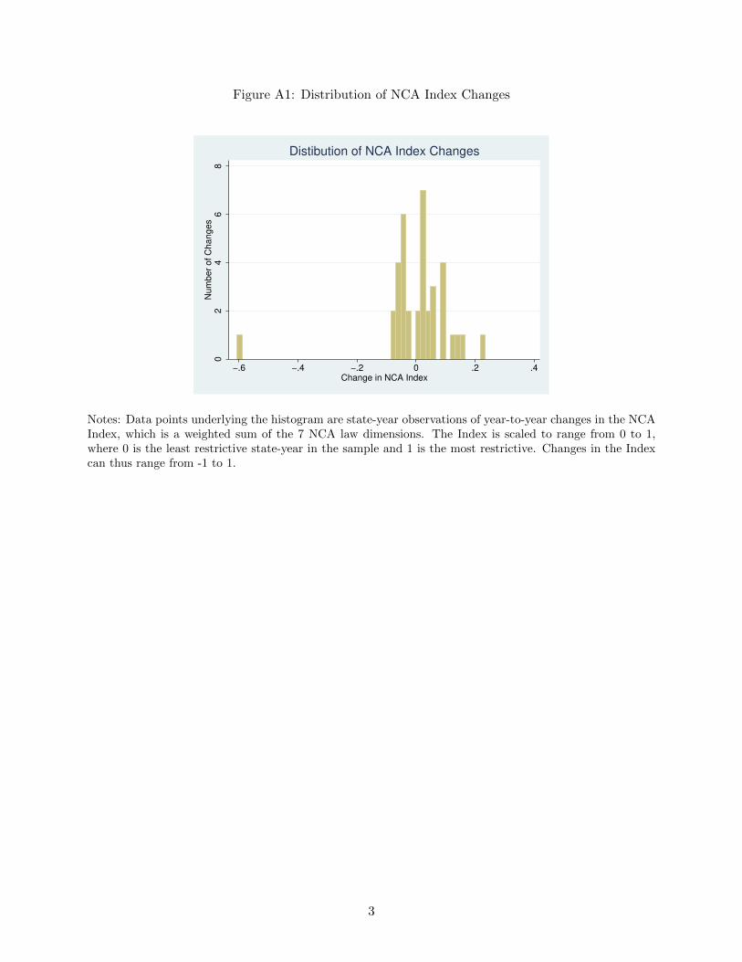
Figure A1: Distribution of NCA Index Changes
02
46
8N
um
ber
of C
hanges
−.6 −.4 −.2 0 .2 .4Change in NCA Index
Distibution of NCA Index Changes
Notes: Data points underlying the histogram are state-year observations of year-to-year changes in the NCAIndex, which is a weighted sum of the 7 NCA law dimensions. The Index is scaled to range from 0 to 1,where 0 is the least restrictive state-year in the sample and 1 is the most restrictive. Changes in the Indexcan thus range from -1 to 1.
3

Table A3: NCA Law Components: Descriptive Statistics
Mean SD N (State-Years)
Statutory Index 0.55 0.24 612Protectible Interest Index 0.60 0.24 605Burden of Proof Index 0.57 0.27 602Consideration Index Inception 0.84 0.30 563Consideration Index Post-Inception 0.70 0.33 526Blue Pencil Index 0.53 0.34 538Employer Termination Index 0.62 0.30 408
Notes: Statistics in the table represent data from 1996-2007 for each state-year in which a legal precedent exists. Theminimum of each component is 0 and the maximum of each component is normalized to 1.
4

Table A4: IV First Stage: Effect of NCA Laws on Establishment-Based Market Concentration
Dependent Variable: HHIt−1
(1) (2) (3)
Statutory Indext−1 0.42 1.80(1.38) (1.99)
Protectible Interest Indext−1 12.16* 8.05*(3.51) (3.95)
Consideration Index Inceptiont−1 21.71 15.22(38.57) (41.59)
Consideration Index Post-Inceptiont−1 –2.46* –1.27(0.34) (0.64)
Burden of Proof Indext−1 –20.70 –13.90(30.66) (33.39)
Blue Pencil Indext−1 12.56* 0.99(3.90) (2.29)
Employer Termination Indext−1 –19.15* –11.17*(4.51) (4.41)
Statutory Indext−2 –2.15 –1.85(1.14) (1.77)
Protectible Interest Indext−2 6.55* 2.92*(1.48) (1.13)
Consideration Index Inceptiont−2 –3.98* 0.36(1.39) (1.15)
Consideration Index Post-Inceptiont−2 –2.54* –1.55*(0.36) (0.61)
Burden of Proof Indext−2 –1.99 –3.70*(1.34) (0.82)
Blue Pencil Indext−2 16.77* 16.18*(2.75) (2.29)
Employer Termination Indext−2 –6.71* –1.62(1.77) (1.25)
N 3,026,780 3,026,780 3,026,780N Clusters 121 121 121R-Sq 0.75 0.75 0.75AP F-Stat 86.85 110.45 460.22
Notes: All specifications include fixed effects for county, census division by year, procedure code (CPT), physicianspecialty, and facility type. All independent variables are scaled to range between 0 and 1, where 1 is the strongestobserved measure of the variable in any state and year in the data. HHI is calculated from establishment sizes inMPIER data, provided by CMS. HHI is scaled to range from 0 to 100, so that a 1 unit change in HHI correspondsto a 100 point change in the typical 10,000 point scale. All standard errors are clustered by state-year. * indicatessignificance at the 0.05 level.
5
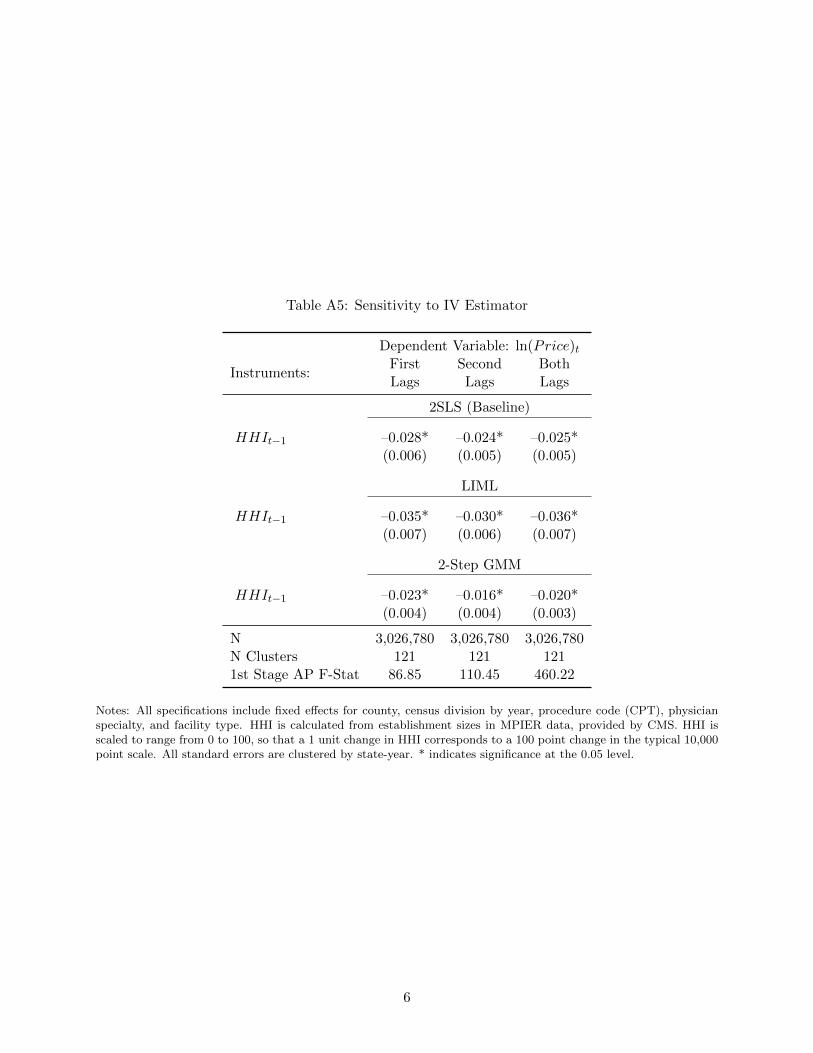
Table A5: Sensitivity to IV Estimator
Dependent Variable: ln(Price)t
Instruments:First Second BothLags Lags Lags
2SLS (Baseline)
HHIt−1 –0.028* –0.024* –0.025*(0.006) (0.005) (0.005)
LIML
HHIt−1 –0.035* –0.030* –0.036*(0.007) (0.006) (0.007)
2-Step GMM
HHIt−1 –0.023* –0.016* –0.020*(0.004) (0.004) (0.003)
N 3,026,780 3,026,780 3,026,780N Clusters 121 121 1211st Stage AP F-Stat 86.85 110.45 460.22
Notes: All specifications include fixed effects for county, census division by year, procedure code (CPT), physicianspecialty, and facility type. HHI is calculated from establishment sizes in MPIER data, provided by CMS. HHI isscaled to range from 0 to 100, so that a 1 unit change in HHI corresponds to a 100 point change in the typical 10,000point scale. All standard errors are clustered by state-year. * indicates significance at the 0.05 level.
6

Table A6: IV Second Stage Estimates: MPIER HHIs, Markets defined by county only
Dependent Variable: ln(Price)IV IV IV OLS
Instruments:First Second BothLags Lags Lags
HHI(t−1) –0.011* –0.015* –0.011* 0.000
(0.050) (0.005) (0.005) (0.000)
N 3,243,820 3,243,820 3,243,820 3,243,820N Clusters 121 121 121 1211st Stage AP F-Stat 29.03 53.70 168.33
Notes:All specifications include fixed effects for county, census division by year, procedure code (CPT), physicianspecialty, and facility type. Markets are defined by county only, and are not differentiated by physician specialty.HHI is calculated from establishment sizes in MPIER data, provided by CMS. HHI is scaled to range from 0 to 100,so that a 1 unit change in HHI corresponds to a 100 point change in the typical 10,000 point scale. All standarderrors are clustered by state-year. * indicates significance at the 0.05 level.
7

Table A7: IV Estimates Dropping Largest NCA Law Changes
Dependent Variable: ln(Price)t(1) (2) (3)
HHIt−1 –0.0263* –0.0212* –0.0218*(0.0052) (0.0041) (0.0039)
Instruments First Lags Second Lags Both Lags
N 2,853,469 2,853,469 2,853,469N Clusters 111 111 1111st Stage AP F-Stat 92.47 119.33 470.95
Notes: All specifications include fixed effects for county, census division by year, procedure code (CPT), physicianspecialty, and facility type. HHI is calculated from establishment sizes in MPIER data, provided by CMS. HHI isscaled to range from 0 to 100, so that a 1 unit change in HHI corresponds to a 100 point change in the typical 10,000point scale. The sample excludes state-years with the largest law changes, which account for 6.3% of the main sample.All standard errors are clustered by state-year. * indicates significance at the 0.05 level.
8

Tab
leA
8:IV
Sec
ond
Sta
geE
stim
ates
for
Alt
ern
ativ
eM
PIE
RH
HI
Mea
sure
s
Dep
end
ent
Var
iab
le:
ln(Price
)(1
)(2
)(3
)(4
)(5
)(6
)(7
)(8
)
HH
I (t−
1)
–0.0
25*
–0.0
16*
–0.0
14*
–0.0
14*
–0.0
22*
–0.0
22*
–0.
020
*–0
.020*
(0.0
05)
(0.0
03)
(0.0
04)
(0.0
03)
(0.0
07)
(0.0
07)
(0.0
08)
(0.0
08)
N3,
026,7
803,
026,
780
2,93
6,69
42,
936,
694
3,02
6,78
03,
026,
780
2,9
36,
694
2,9
36,
694
NC
lust
ers
121
121
121
121
121
121
121
121
R-S
q0.9
80.
980.
980.
980.
980.
98
0.98
0.98
1st
Sta
ge
AP
F-S
tat
460.2
270
4.58
1735
.79
868.
5671
0.56
816
.02
498.
02
598.
01
Note
s:A
llsp
ecifi
cati
ons
incl
ude
fixed
effec
tsfo
rco
unty
,ce
nsu
sdiv
isio
nby
yea
r,pro
cedure
code
(CP
T),
physi
cian
spec
ialt
y,and
faci
lity
typ
e.H
HI
isca
lcula
ted
from
esta
blish
men
tsi
zes
inM
PIE
Rdata
,pro
vid
edby
CM
S.
Inco
lum
n(1
)th
eH
HI
ism
easu
red
incl
udin
gall
physi
cians
inany
gro
up
that
has
at
least
one
mem
ber
ina
giv
ensp
ecia
lty,
and
ass
um
esphysi
cians
wit
hm
issi
ng
addre
sses
are
solo
esta
blish
men
ts.
The
HH
Iin
colu
mn
(1)
isth
eone
use
dth
roughout
the
pap
er.
The
HH
Iin
colu
mn
(2)
issi
milar
toth
at
inco
lum
n(1
),but
ass
um
esall
physi
cians
ina
giv
enm
ark
etw
ith
mis
sing
addre
sses
are
inth
esa
me
esta
blish
men
t.In
colu
mn
(3)
the
HH
Iis
mea
sure
din
cludin
gall
physi
cians
inany
gro
up
that
has
at
least
one
mem
ber
ina
giv
ensp
ecia
lty,
dro
ps
obse
rvati
ons
wit
hm
issi
ng
addre
sses
ifth
esa
me
physi
cian
has
anoth
erknow
naddre
ssin
the
sam
ezi
pco
de,
and
ass
um
esall
rem
ain
ing
mis
sing
addre
sses
are
solo
esta
blish
men
ts.
The
HH
Iin
colu
mn
(4)
issi
milar
toth
at
inco
lum
n(3
),but
ass
um
esall
rem
ain
ing
mis
sing
addre
sses
ina
giv
enm
ark
etare
asi
ngle
esta
blish
men
t.In
colu
mn
(5)
the
HH
Iis
mea
sure
din
cludin
gonly
physi
cians
inth
egiv
ensp
ecia
lty
wit
hin
the
mark
et,
and
ass
um
esphysi
cians
wit
hm
issi
ng
addre
sses
are
solo
esta
blish
men
ts.
The
HH
Iin
colu
mn
(6)
issi
milar
toth
at
inco
lum
n(5
),but
ass
um
esall
physi
cians
ina
giv
enm
ark
etw
ith
mis
sing
addre
sses
are
inth
esa
me
esta
blish
men
t.In
colu
mn
(7)
the
HH
Iis
mea
sure
din
cludin
gonly
physi
cians
inth
egiv
ensp
ecia
lty
wit
hin
the
mark
et,
dro
ps
obse
rvati
ons
wit
hm
issi
ng
addre
sses
ifth
esa
me
physi
cian
has
anoth
erknow
naddre
ssin
the
sam
ezi
pco
de,
and
ass
um
esall
rem
ain
ing
mis
sing
addre
sses
are
solo
esta
blish
men
ts.
The
HH
Iin
colu
mn
(8)
issi
milar
toth
at
inco
lum
n(7
),but
ass
um
esall
rem
ain
ing
mis
sing
addre
sses
ina
giv
enm
ark
etare
asi
ngle
esta
blish
men
t.A
llH
HIs
are
scale
dto
range
from
0to
100,
soth
at
a1
unit
change
inH
HI
corr
esp
onds
toa
100
poin
tch
ange
inth
ety
pic
al
10,0
00
poin
tsc
ale
.In
each
spec
ifica
tion,
the
inst
rum
ents
incl
ude
all
lagged
and
twic
ela
gged
law
com
ponen
ts(c
orr
esp
ondin
gto
colu
mn
3in
Table
7).
All
standard
erro
rscl
ust
ered
by
state
-yea
r.*
indic
ate
ssi
gnifi
cance
at
the
0.0
5le
vel
.
9
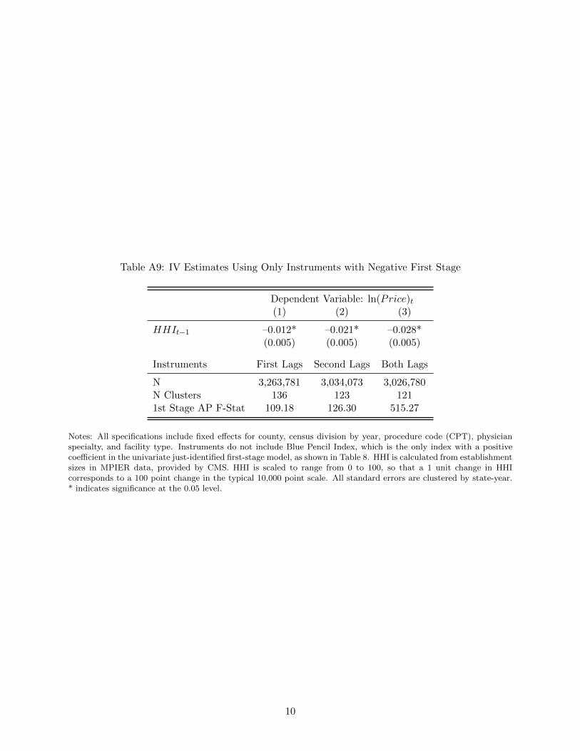
Table A9: IV Estimates Using Only Instruments with Negative First Stage
Dependent Variable: ln(Price)t(1) (2) (3)
HHIt−1 –0.012* –0.021* –0.028*(0.005) (0.005) (0.005)
Instruments First Lags Second Lags Both Lags
N 3,263,781 3,034,073 3,026,780N Clusters 136 123 1211st Stage AP F-Stat 109.18 126.30 515.27
Notes: All specifications include fixed effects for county, census division by year, procedure code (CPT), physicianspecialty, and facility type. Instruments do not include Blue Pencil Index, which is the only index with a positivecoefficient in the univariate just-identified first-stage model, as shown in Table 8. HHI is calculated from establishmentsizes in MPIER data, provided by CMS. HHI is scaled to range from 0 to 100, so that a 1 unit change in HHIcorresponds to a 100 point change in the typical 10,000 point scale. All standard errors are clustered by state-year.* indicates significance at the 0.05 level.
10
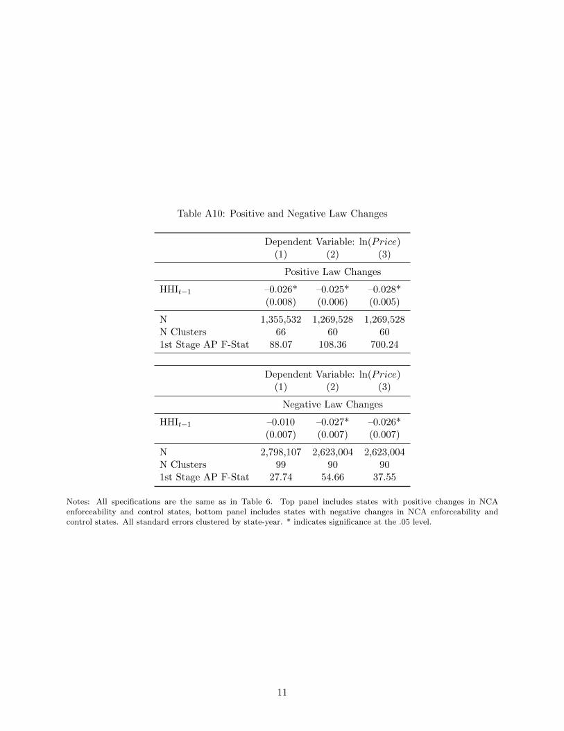
Table A10: Positive and Negative Law Changes
Dependent Variable: ln(Price)(1) (2) (3)
Positive Law Changes
HHIt−1 –0.026* –0.025* –0.028*(0.008) (0.006) (0.005)
N 1,355,532 1,269,528 1,269,528N Clusters 66 60 601st Stage AP F-Stat 88.07 108.36 700.24
Dependent Variable: ln(Price)(1) (2) (3)
Negative Law Changes
HHIt−1 –0.010 –0.027* –0.026*(0.007) (0.007) (0.007)
N 2,798,107 2,623,004 2,623,004N Clusters 99 90 901st Stage AP F-Stat 27.74 54.66 37.55
Notes: All specifications are the same as in Table 6. Top panel includes states with positive changes in NCAenforceability and control states, bottom panel includes states with negative changes in NCA enforceability andcontrol states. All standard errors clustered by state-year. * indicates significance at the .05 level.
11

Table A11: Interactions between Physician and Insurer Concentration
Dependent Variable: ln(Price)t(1) (2) (3)
Phys HHIt−1 –0.024* –0.025* –0.025*(0.004) (0.005) (0.006)
Phys HHIt−1 × I(Ins HHI > 2500) –0.001(0.002)
Phys HHIt−1 × I(Ins HHI > 4000) 0.002(0.002)
Phys HHIt−1 × I(Ins HHI < 2500) 0.002(0.002)
Phys HHIt−1 × I(Ins HHI > 5000) 0.000(0.002)
N 3,026,780 3,026,780 3,026,780N Clusters 121 121 1211st Stage F-Stat 297.13 338.98 245.75
Notes: All specifications include fixed effects for county, census division by year, procedure code (CPT), physicianspecialty, and facility type. Physician HHIs are calculated from establishment sizes in MPIER data, insurer HHIsare state-level measures in 2007 from the AMA. HHI is scaled to range from 0 to 100, so that a 1 unit change in HHIcorresponds to a 100 point change in the typical 10,000 point scale. All standard errors are clustered by state-year.Kleinbergen-Paap F-Statistics reported. * indicates significance at the 0.05 level.
12

Table A12: Effect of Concentration on Prices, by Medical Specialty and Urban Status
Dependent Variable: ln(Price)tAll Counties Metro Counties Non-Metro Counties
InstrumentsFirst First and First First and First First andLags Second Lags Lags Second Lags Lags Second Lags(1) (2) (3) (4) (5) (6)
All PhysiciansHHIt−1 –0.028* –0.025* –0.034* –0.031* –0.013* –0.011*
(0.006) (0.005) (0.006) (0.006) (0.006) (0.005)N 3,026,780 3,026,780 2,077,627 2,077,627 949,153 949,1531st Stage AP F-Stat 86.9 460.2 54.7 364.3 15.4 15.1
Primary Care PhysiciansHHIt−1 –0.024* –0.017* –0.036* –0.026* –0.007 –0.006
(0.005) (0.005) (0.008) (0.006) (0.004) (0.003)N 473,033 473,033 306,449 306,449 166,584 166,5841st Stage AP F-Stat 47.2 542.3 22.8 458.0 14.9 12.2
Non-Surgical SpecialistsHHIt−1 –0.013* –0.013* –0.026* –0.023* 0.001 0.000
(0.003) (0.003) (0.004) (0.004) (0.002) (0.002)N 300,990 300,990 234,402 234,402 66,588 66,5881st Stage AP F-Stat 39.2 98.3 84.4 277.8 31.2 21.8
Surgical SpecialistsHHIt−1 –0.004 –0.005 –0.009 –0.009 –0.000 –0.003
(0.007) (0.005) (0.006) (0.005) (0.008) (0.003)N 272,913 272,913 191,790 191,790 81,123 81,1231st Stage AP F-Stat 8.3 17.2 29.21 55.0 1.1 2.4
Notes: All specifications include fixed effects for county, census division by year, procedure code (CPT), physicianspecialty, and facility type. HHI is calculated from establishment sizes in MPIER data, provided by CMS. HHI isscaled to range from 0 to 100, so that a 1 unit change in HHI corresponds to a 100 point change in the typical 10,000point scale. All estimates represent the second stage coefficient on HHI in 2SLS models corresponding to those incolumns (1) and (3) of Table 7 for all counties, metro counties, and non-metro counties. The first two columns of thefirst panel reproduce the second stage results for all physicians in Table 7. The ‘Primary Care Physicians’ sampleincludes primary care MDs (excluding DOs), Internal Medicine, Family Practice, Geriatric Medicine, and Pediatricspecialists. The ‘Non-Surgical Specialist’ sample includes specialists in Proctology, Urology, Dermatology, Cardio-vascular Dis/Cardiology, Neurology, Gastroenterology, and Hematology. The ‘Surgical Specialist’ sample includesspecialists in General Surgery, Neurological Surgery, Orthopaedic Surgery, Thoracic Surgery, Anesthesiology, andRadiology. All standard errors are clustered by state-year. * indicates significance at the 0.05 level.
13
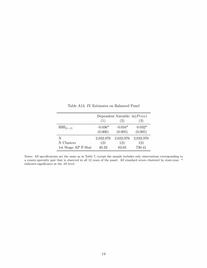
Table A13: IV Estimates on Balanced Panel
Dependent Variable: ln(Price)(1) (2) (3)
HHI(t−1) –0.036* –0.034* –0.032*
(0.006) (0.005) (0.005)
N 2,032,976 2,032,976 2,032,976N Clusters 121 121 1211st Stage AP F-Stat 40.33 83.65 730.41
Notes: All specifications are the same as in Table 7, except the sample includes only observations corresponding toa county-specialty pair that is observed in all 12 years of the panel. All standard errors clustered by state-year. *indicates significance at the .05 level.
14

Table A14: Sensitivity of MPIER Second Stage IV Estimates to Fuzzy Matching AlgorithmParameter
Normalized LevenshteinIV Estimate
First StageDistance Threshold AP F-Stat.
0.01–0.026*
516.27(0.005)
0.05–0.025*
535.96(0.005)
0.10–0.025*
489.11(0.005)
0.15–0.026*
478.49(0.005)
0.20–0.025*
460.22(0.005)
0.25–0.027*
530.28(0.005)
0.30–0.026*
613.38(0.005)
0.35–0.026*
607.27(0.005)
0.40–0.026*
587.15(0.005)
Notes: All specifications include fixed effects for county, census division by year, procedure code (CPT), physicianspecialty, and facility type. IVs are the full set of first and second lags of law components. The normalized LevenshteinDistance equals the minimum number of character insertions, deletions, or substitutions necessary to make two stringsequal, divided by the length of the shorter string. The threshold value is the value of the normalized Levenshteindistance below which the character elements of two addresses in the MPIER are assumed to be equivalent. Alarger threshold value results in over-estimating the size of establishments, while too low a value in the presence oftypographical errors may lead to an underestimate of establishment sizes. The main estimates in the paper are basedon a threshold value of 0.20. HHI is calculated from establishment sizes in MPIER data, provided by CMS. HHI isscaled to range from 0 to 100, so that a 1 unit change in HHI corresponds to a 100 point change in the typical 10,000point scale. All standard errors are clustered by state-year. * indicates significance at the 0.05 level.
15
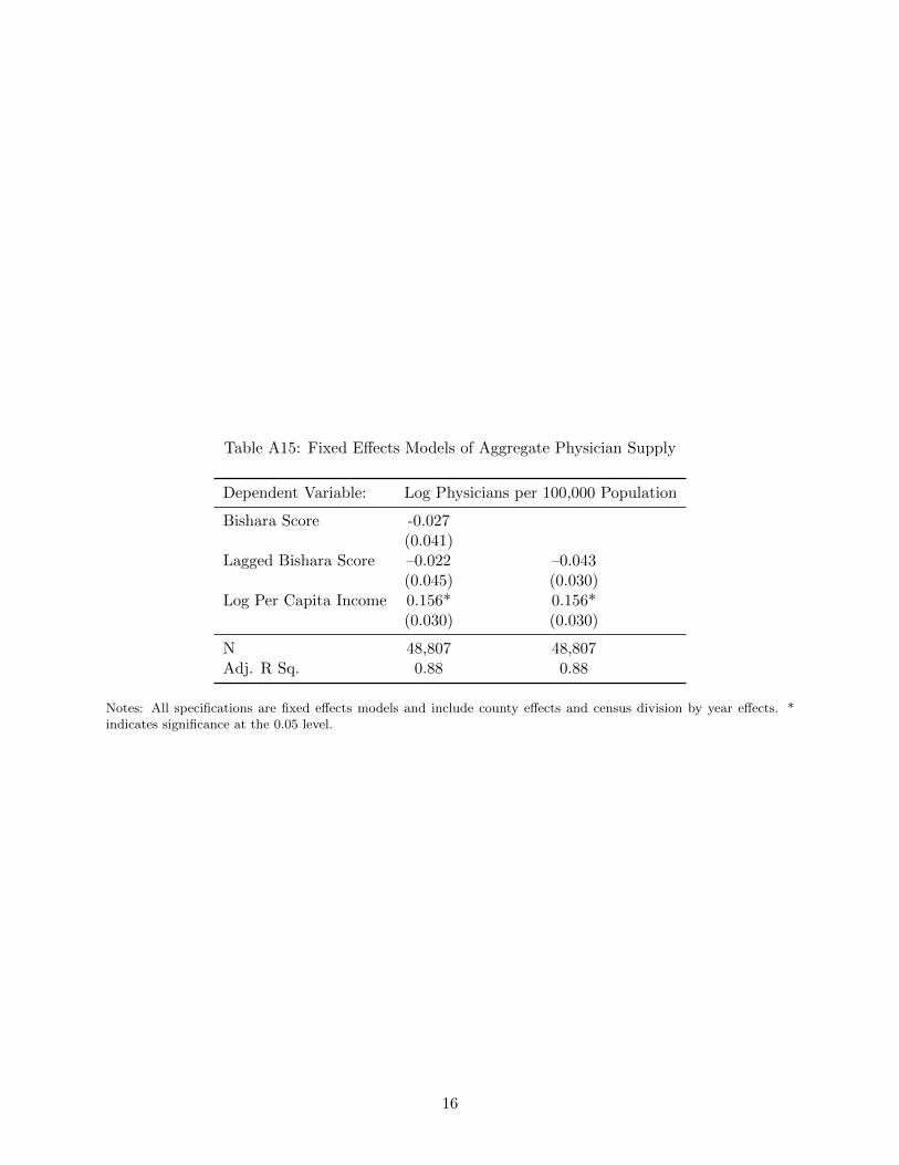
Table A15: Fixed Effects Models of Aggregate Physician Supply
Dependent Variable: Log Physicians per 100,000 Population
Bishara Score -0.027(0.041)
Lagged Bishara Score –0.022 –0.043(0.045) (0.030)
Log Per Capita Income 0.156* 0.156*(0.030) (0.030)
N 48,807 48,807Adj. R Sq. 0.88 0.88
Notes: All specifications are fixed effects models and include county effects and census division by year effects. *indicates significance at the 0.05 level.
16
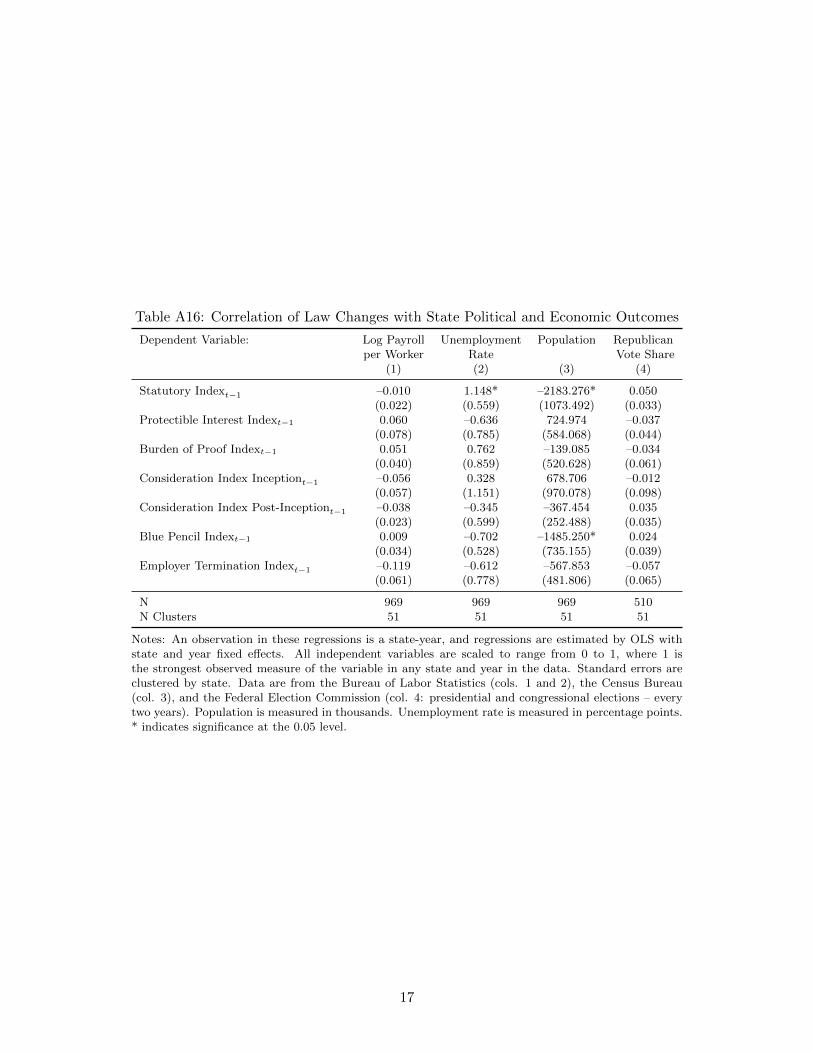
Table A16: Correlation of Law Changes with State Political and Economic Outcomes
Dependent Variable: Log Payroll Unemployment Population Republicanper Worker Rate Vote Share
(1) (2) (3) (4)
Statutory Indext−1 –0.010 1.148* –2183.276* 0.050(0.022) (0.559) (1073.492) (0.033)
Protectible Interest Indext−1 0.060 –0.636 724.974 –0.037(0.078) (0.785) (584.068) (0.044)
Burden of Proof Indext−1 0.051 0.762 –139.085 –0.034(0.040) (0.859) (520.628) (0.061)
Consideration Index Inceptiont−1 –0.056 0.328 678.706 –0.012(0.057) (1.151) (970.078) (0.098)
Consideration Index Post-Inceptiont−1 –0.038 –0.345 –367.454 0.035(0.023) (0.599) (252.488) (0.035)
Blue Pencil Indext−1 0.009 –0.702 –1485.250* 0.024(0.034) (0.528) (735.155) (0.039)
Employer Termination Indext−1 –0.119 –0.612 –567.853 –0.057(0.061) (0.778) (481.806) (0.065)
N 969 969 969 510N Clusters 51 51 51 51
Notes: An observation in these regressions is a state-year, and regressions are estimated by OLS withstate and year fixed effects. All independent variables are scaled to range from 0 to 1, where 1 isthe strongest observed measure of the variable in any state and year in the data. Standard errors areclustered by state. Data are from the Bureau of Labor Statistics (cols. 1 and 2), the Census Bureau(col. 3), and the Federal Election Commission (col. 4: presidential and congressional elections – everytwo years). Population is measured in thousands. Unemployment rate is measured in percentage points.* indicates significance at the 0.05 level.
17

Tab
leA
17:
Cor
rela
tion
ofL
awC
han
ges
wit
hP
olit
ical
and
Eco
nom
icV
iew
sin
the
GS
S
Dep
enden
tV
ari
able
:R
esp
onden
tT
hin
ks
The
Res
ponden
tT
hin
ks
We
are
Gov
ernm
ent
Should
Do
Les
s:Sp
endin
gto
oM
uch
On:
Res
ponden
tC
onsi
der
sH
imse
lf:
To
Hel
pSati
sfied
Wit
hP
ayfo
rN
ati
on’s
His
Fin
aci
al
InG
ener
al
Med
ical
Care
Urb
an
Issu
esW
elfa
reH
ealt
hA
Rep
ublica
nSit
uati
on
(1)
(2)
(3)
(4)
(5)
(6)
(7)
Sta
tuto
ryIn
dex
t−1
0.3
16
0.0
31
–0.1
66
–0.1
02
–0.1
21
–0.0
09
–0.2
97
(0.1
77)
(0.1
20)
(0.2
57)
(0.3
22)
(0.1
55)
(0.1
69)
(0.2
16)
Pro
tect
ible
Inte
rest
Index
t−1
–0.0
26
0.0
74
–0.4
27
–0.5
13
0.0
21
–0.3
31
–0.0
74
(0.3
76)
(0.1
96)
(0.3
72)
(0.4
62)
(0.2
10)
(0.3
65)
(0.3
63)
Burd
enof
Pro
of
Index
t−1
–0.1
03
–0.0
31
–0.6
85
0.3
94
0.2
15
–0.1
41
–0.4
54
(0.3
83)
(0.3
60)
(0.5
15)
(0.7
45)
(0.3
43)
(0.5
02)
(0.3
17)
Consi
der
ati
on
Index
Ince
pti
ont−
10.0
29
–0.0
92
0.8
19
–0.1
64
–0.4
53
0.4
63
0.5
27
(0.4
38)
(0.3
40)
(0.5
58)
(0.7
58)
(0.3
47)
(0.5
02)
(0.4
22)
Consi
der
ati
on
Index
Post
-Ince
pti
ont−
10.1
44
–0.1
31
–0.0
34
0.1
51
0.5
46*
–0.0
62
0.0
01
(0.1
23)
(0.0
86)
(0.4
07)
(0.2
44)
(0.2
08)
(0.2
71)
(0.2
37)
Blu
eP
enci
lIn
dex
t−1
–0.2
97
0.3
65
–0.0
26
–0.1
21
0.2
68
–0.2
97
0.2
28
(0.3
39)
(0.2
40)
(0.4
68)
(0.4
74)
(0.3
17)
(0.4
05)
(0.5
35)
Em
plo
yer
Ter
min
ati
on
Index
t−1
0.8
17
0.7
38
–0.9
74
–0.1
97
0.2
37
–0.3
25
0.6
31
(0.5
32)
(0.5
68)
(0.4
84)
(0.7
91)
(0.5
90)
(0.5
38)
(1.0
06)
N1,0
26
1,0
26
1,0
26
1,0
26
1,0
26
1,0
26
1,0
26
NC
lust
ers
28
28
28
28
28
28
28
Note
s:R
egre
ssio
ns
are
linea
rpro
babilit
ym
odel
sin
whic
han
obse
rvati
on
isa
surv
eyre
sponden
tin
agiv
enyea
rand
ap
osi
tive
outc
om
ere
pre
sents
the
resp
onden
t’s
agre
emen
tw
ith
the
state
men
tpre
sente
din
each
colu
mn.
All
regre
ssio
ns
incl
ude
state
,yea
r,occ
upati
on,
and
indust
ryfixed
effec
ts,
as
wel
las
contr
ols
for
age,
educa
tion,
mari
tal
statu
s,and
emplo
ym
ent
statu
s.A
llin
dep
enden
tva
riable
sare
scale
dto
range
from
0to
1,
wher
e1
isth
est
ronges
tobse
rved
mea
sure
of
the
vari
able
inany
state
and
yea
rin
the
data
.Sta
ndard
erro
rsare
clust
ered
by
state
.D
ata
on
politi
cal
and
econom
icvie
ws
are
taken
from
the
Gen
eralize
dSoci
al
Surv
eyfo
rth
eyea
rs1993-2
010,
wher
edata
exis
t(a
ppro
xim
ate
lyev
ery
oth
eryea
rand
inonly
28
state
s).
*in
dic
ate
ssi
gnifi
cance
at
the
0.0
5le
vel
.
18