physico-chemical parameters and ...studentsrepo.um.edu.my/9178/2/physico-chemical_parameters...iv...
TRANSCRIPT

PHYSICO-CHEMICAL PARAMETERS AND MACROBENTHOS OF PENCHALA RIVER
ROSE FADZILAH BINTI ABDULLAH
FACULTY OF SCIENCE
UNIVERSITY OF MALAYA KUALA LUMPUR
2017

PHYSICO-CHEMICAL PARAMETERS AND
MACROBENTHOS OF PENCHALA RIVER
ROSE FADZILAH BINTI ABDULLAH
DISSERTATION SUBMITTED IN PARTIAL
FULFILMENT OF THE REQUIREMENTS FOR THE
DEGREE OF MASTER OF TECHNOLOGY
INSTITUTE OF BIOLOGICAL SCIENCE
UNIVERSITY OF MALAYA
KUALA LUMPUR
2017

ii
UNIVERSITY OF MALAYA
ORIGINAL LITERARY WORK DECLARATION
Name of Candidate: ROSE FADZILAH BINTI ABDULLAH
(I.C/Passport No: 890402-06-5104)
Matric No: SGH110019
Name of Degree: MASTER OF TECHNOLOGY
(ENVIRONMENT MANAGEMENT)
Title of Project Paper/Research Report/Dissertation/Thesis (“this Work”):
PHYSICO-CHEMICAL PARAMETERS AND MACROBENTHOS OF
PENCHALA RIVER
Field of Study: WATER QUALITY
I do solemnly and sincerely declare that:
(1) I am the sole author/writer of this Work;
(2) This Work is original;
(3) Any use of any work in which copyright exists was done by way of fair dealing
and for permitted purposes and any excerpt or extract from, or reference to or
reproduction of any copyright work has been disclosed expressly and
sufficiently and the title of the Work and its authorship have been
acknowledged in this Work;
(4) I do not have any actual knowledge nor do I ought reasonably to know that the
making of this work constitutes an infringement of any copyright work;
(5) I hereby assign all and every rights in the copyright to this Work to the
University of Malaya (“UM”), who henceforth shall be owner of the copyright
in this Work and that any reproduction or use in any form or by any means
whatsoever is prohibited without the written consent of UM having been first
had and obtained;
(6) I am fully aware that if in the course of making this Work I have infringed any
copyright whether intentionally or otherwise, I may be subject to legal action
or any other action as may be determined by UM.
Candidate’s Signature Date:
Subscribed and solemnly declared before,
Witness’s Signature Date:
Name:
Designation:

ii
UNIVERSITI MALAYA
PERAKUAN KEASLIAN PENULISAN
Nama: ROSE FADZILAH BINTI ABDULLAH
(No. K.P/Pasport: 890402-06-5104)
No. Matrik: SGH110019
Nama Ijazah: SARJANA TEKNOLOGI (PENGURUSAN ALAM SEKITAR)
Tajuk Kertas Projek/Laporan Penyelidikan/Disertasi/Tesis (“Hasil Kerja ini”):
PARAMETER FISIKO-KIMIA DAN MAKROBENTIK DI SUNGAI
PENCHALA
Bidang Penyelidikan: KUALITI AIR
Saya dengan sesungguhnya dan sebenarnya mengaku bahawa:
(1) Saya adalah satu-satunya pengarang/penulis Hasil Kerja ini;
(2) Hasil Kerja ini adalah asli;
(3) Apa-apa penggunaan mana-mana hasil kerja yang mengandungi hakcipta telah
dilakukan secara urusan yang wajar dan bagi maksud yang dibenarkan dan apa-
apa petikan, ekstrak, rujukan atau pengeluaran semula daripada atau kepada
mana-mana hasil kerja yang mengandungi hakcipta telah dinyatakan dengan
sejelasnya dan secukupnya dan satu pengiktirafan tajuk hasil kerja tersebut dan
pengarang/penulisnya telah dilakukan di dalam Hasil Kerja ini;
(4) Saya tidak mempunyai apa-apa pengetahuan sebenar atau patut
semunasabahnya tahu bahawa penghasilan Hasil Kerja ini melanggar suatu
hakcipta hasil kerja yang lain;
(5) Saya dengan ini menyerahkan kesemua dan tiap-tiap hak yang terkandung di
dalam hak cipta Hasil Kerja ini kepada Universiti Malaya (“UM”) yang
seterusnya mula darisekarang adalah tuan punya kepada hakcipta di dalam
Hasil Kerja ini dan apa-apa pengeluaran semula atau penggunaan dalam apa
jua bentuk atau dengan apa juga cara sekalipun adalah dilarang tanpa terlebih
dahulu mendapat kebenaran bertulis dari UM;
(6) Saya sedar sepenuhnya sekiranya dalam masa penghasilan Hasil Kerja ini saya
telah melanggar suatu hakcipta hasil kerja yang lain sama ada dengan niat atau
sebaliknya,saya boleh dikenakan tindakan undang-undang atau apa-apa
tindakan lain sebagaimana yang diputuskan oleh UM.
Tandatangan Calon Tarikh:
Diperbuat dan sesungguhnya diakui di hadapan,
Tandatangan Saksi Tarikh:
Nama:
Jawatan:

iii
ABSTRACT
The aim of this study is to determine the relationship between physico-chemical
parameters with existence and diversity of macrobenthos at four selected stations at
Penchala River. WQI was determined by analysing water samples through water
sampling routine for 12 months starting November 2013 until October 2014. In situ
measurements involved were temperature, pH, dissolved oxygen (DO), total dissolved
solid (TDS), and conductivity. Laboratory analysis was undertaken for total suspended
solid (TSS), Biological Oxygen Demand (BOD), Chemical Oxygen Demand (COD), and
Ammoniacal Nitrogen (NH3-N). Measurements for physical parameters were done for
water level, river width, and river water velocity. The WQI value Penchala River were in
the range of 58.1 – 71.0. Station 2, 3, 4 received pollutant from difference sources such
as residential, commercial and industrial area which discharged high concentration of
nutrients and organic pollutant. The natural physical characteristics at Station 1 encourage
the existence and support high diversity of macrobenthos. The deterioration of water
quality, velocity and water level thus affected the existence of macrobenthos at Station 2,
3 and 4. The Pearson’s correlation of coefficients shows high correlation between WQI
and Margalef richness index (r= -0.735, P=0.007), Simpsons diversity index (r= -0.618,
P=0.032), Shannon-Weiner diversity index (r= -0.642, P=0.024) and Pielou evenness
index (r= -0.589, P=0.044) indicate that biological monitoring at Penchala River by using
macrobenthos is suitable as an alternative way to determine the river health.

iv
ABSTRAK
Tujuan kajian ini adalah untuk menentukan hubungan antara parameter fizikal-kimia
dengan kewujudan dan kepelbagaian makrobentik di empat stesen terpilih di Penchala
River. Indeks kualiti air ditentukan bermula November 2013 sehingga Oktober 2014.
Dalam ukuran in-situ, parameter yang terlibat adalah suhu, pH, oksigen terlarut (DO),
jumlah pepejal terlarut (TDS), dan kekonduksian. Analisis makmal telah dijalankan bagi
jumlah pepejal terampai (TSS), Biological Oxygen Demand (BOD), Chemical Oxygen
Demand (COD), dan Ammoniakal Nitrogen (NH3- N). Pengukuran parameter fizikal
dilakukan untuk paras air, lebar sungai dan halaju air sungai. Indeks kualiti air di Sungai
Penchala adalah dalam lingkungan 58.1 – 71.0. Stesen 2, 3, 4 menerima pencemaran
daripada kawasan kediaman, perdagangan dan perindustrian dengan jumlah kepekatan
nutrien dan bahan organik yang tinggi. Daripada pemerhatian, ciri-ciri fizikal semulajadi
di Stesen 1 sangat menggalakkan kewujudan makrobentik. Berbanding dengan Stesen 2,
3 dan 4, gangguan yang berlaku tertahap kualiti air, halaju dan aras air telah memberikan
kesan negatif kepada kewujudan makrobentik. Analisis korelasi Pearson menunjukkan
hubungan yang kuat antara indeks kualiti air dengan indeks kekayaan Margalef
(r= -0.735, P=0.007), indeks kepelbagaian Simpson (r= -0.618, P=0.032), indeks
kepelbagaian Shannon-Weiner (r= -0.642, P=0.024) dan indeks kesamarataan Pielou
(r= -0.589, P=0.044) membuktikan bahawa pemantauan biologi di Penchala River sesuai
dijadikan cara alternatif untuk mendapatkan status kesihatan sungai.

v
ACKNOWLEDGEMENTS
First I would like to express my gratitude to my supervisor Dr Ghufran Redzwan and
Associate Professor Dr Faridah Othman for untiring guidance, intuitive comments,
encouragements, remarks and engagement through the learning process of this master
dissertation.
My heartfelt gratitude also goes out to my course mate which come from my faculty,
Institute of Biological Science, University of Malaya. Those who involve directly or
indirectly the completion of this research. All their help and support are beyond
repayment.
Finally, the project would not have been possible without the unfailing support from
my family members, especially my parents, Encik Abdullah bin Sudin and Puan Zaleha
Idris. I am truly indebted and thankful for their unconditional love and confidence in me
as well as their endless patience and encouragement. I am grateful to my husband, Encik
Mohd Zahid Shamsudin and my bestfriend, Cik Normarina who has supported me
throughout the entire process, both by keeping me harmonious and helping me putting
pieces together.

vi
TABLE OF CONTENTS
Abstract ........................................................................................................................ iii
Abstrak......................................................................................................................... iv
Acknowledgements ...................................................................................................... v
Table of Contents......................................................................................................... vi
List of Figures .............................................................................................................. ix
List of Tables ............................................................................................................... xi
List of Symbols and Abbreviations ............................................................................ xii
List of Appendices ..................................................................................................... xiii
CHAPTER 1: INTRODUCTION .................................................................................. 1
1.1 Background of study ................................................................................................ 1
1.1.1 Overview of urban river ............................................................................. 1
1.1.2 Application of macrobenthos as bioindicator ............................................. 2
1.2 Statement of problem ............................................................................................... 3
1.3 Aim and objectives .................................................................................................. 4
1.4 Scope and limitation ................................................................................................ 6
1.5 Implication by the limitation ................................................................................... 6
CHAPTER 2: LITERATURE REVIEW ...................................................................... 7
2.1 River health for urban river ..................................................................................... 7
2.1.1 Relationship between river health and urban river ..................................... 9
2.2 Threats to urban river............................................................................................. 10
2.2.1 Channelisation .......................................................................................... 10
2.2.2 Extreme increasing and decreasing of water volume ............................... 12
2.2.3 Shallow stream bottom ............................................................................. 13

vii
2.2.4 Loss of riparian vegetation ....................................................................... 13
2.2.5 Degradation of ecosystem services .......................................................... 13
2.3 Managing urban river ............................................................................................ 14
2.4 Water quality control for urban river ..................................................................... 16
2.4.1 Biological indicator for water quality monitoring .................................... 18
2.5 Introduction of macrobenthos as biological indicator to determine water quality 20
2.5.1 Use of macrobenthos as water quality indicator....................................... 22
2.5.2 Levels of tolerance of macrobenthos to water pollution .......................... 23
2.5.3 Diversity indices ....................................................................................... 24
CHAPTER 3: METHODOLOGY ............................................................................... 27
3.1 Introduction............................................................................................................ 27
3.2 Determination of location to represent urban river................................................ 27
3.2.1 Background of Penchala River ................................................................. 28
3.2.2 Selection of sampling sites ....................................................................... 30
3.3 Determination of physico-chemical characteristics ............................................... 33
3.3.1 Sampling technique .................................................................................. 33
3.3.2 Water quality parameters .......................................................................... 34
3.3.3 Physical characteristics ............................................................................. 37
3.4 Sampling of macrobenthos .................................................................................... 38
3.4.1 Site selection for sampling macrobenthos ................................................ 38
3.4.2 Method for sampling macrobenthos ......................................................... 38
3.4.3 Identification of macrobenthos ................................................................. 39
3.5 Measurement of biological indices ........................................................................ 39
3.5.1 Shannon-Weiner Diversity Index ............................................................. 39
3.5.2 Simpson Diversity Index .......................................................................... 40
3.5.3 Margalef Richness Index .......................................................................... 40

viii
3.5.4 Pielou Evenness Index .............................................................................. 41
3.6 Statistical Analysis................................................................................................. 41
CHAPTER 4: RESULTS .............................................................................................. 43
4.1 Physico-chemical characteristics at Penchala River .............................................. 43
4.1.1 Chemical characteristics at Penchala River .............................................. 43
4.1.2 Physical characteristics at Penchala River ............................................... 50
4.2 Abundance and distribution of macrobenthos at Penchala River .......................... 52
4.3 Statistical analysis .................................................................................................. 57
CHAPTER 5: DISCUSSION ....................................................................................... 59
5.1 Variation of physico-chemical parameters at Penchala River ............................... 59
5.2 Variations of macrobenthos at Penchala River ...................................................... 65
5.3 Relationship of physico-chemical parameters and species diversity of
macrobenthos at Penchala River ............................................................................ 66
CHAPTER 6: CONCLUSION ..................................................................................... 74
REFERENCES ........................................................................................................... 77
APPENDIX A............................................................................................................. 95
APPENDIX B ............................................................................................................. 97

ix
LIST OF FIGURES
Figure 3.1: Catchment of Penchala River (Mahazar et al., 2013) ................................... 29
Figure 3.2: Station 1 ........................................................................................................ 31
Figure 3.3: Station 2 ........................................................................................................ 31
Figure 3.4: Station 3 ........................................................................................................ 32
Figure 3.5: Station 4 ........................................................................................................ 32
Figure 4.1: Monthly results of Water Quality Index (WQI) for the average .................. 43
Figure 4.2: Monthly results of DO for the average of four sampling stations of Penchala
River ................................................................................................................................ 45
Figure 4.3: Monthly results of BOD and COD for the average of four sampling stations
of Penchala River ............................................................................................................ 46
Figure 4.4: Monthly results of pH for the average of four sampling stations of Penchala
River ................................................................................................................................ 47
Figure 4.5: Monthly results of NH3-N for the average of four sampling stations of
Penchala River ................................................................................................................ 48
Figure 4.6: Monthly results of TSS for the average of four sampling stations of Penchala
River ................................................................................................................................ 49
Figure 4.7: Monthly results of water level for the average of four sampling stations of
Penchala River ................................................................................................................ 50
Figure 4.8: Monthly results of velocity for the average of four sampling stations of
Penchala River ................................................................................................................ 51
Figure 4.9: Monthly results of discharge for the average of four sampling stations of
Penchala River ................................................................................................................ 52
Figure 4.10: Abundance of macrobenthos at Station 1, 2, 3 and 4 from November 2013
to October 2014 of Penchala River ................................................................................. 55
Figure 4.11: Percentages of macrobenthos collected at Station 1, 2, 3 and 4 of Penchala
River ................................................................................................................................ 55

x
Figure 5.1: Overflow at Station 1 during construction in September 2014 .................... 60
Figure 5.2: White boulders at Station 2 during construction in January 2014 ................ 64

xi
LIST OF TABLES
Table 2.1: General pollution tolerance for common macrobenthos (Carter and Resh,
2013) ............................................................................................................................... 24
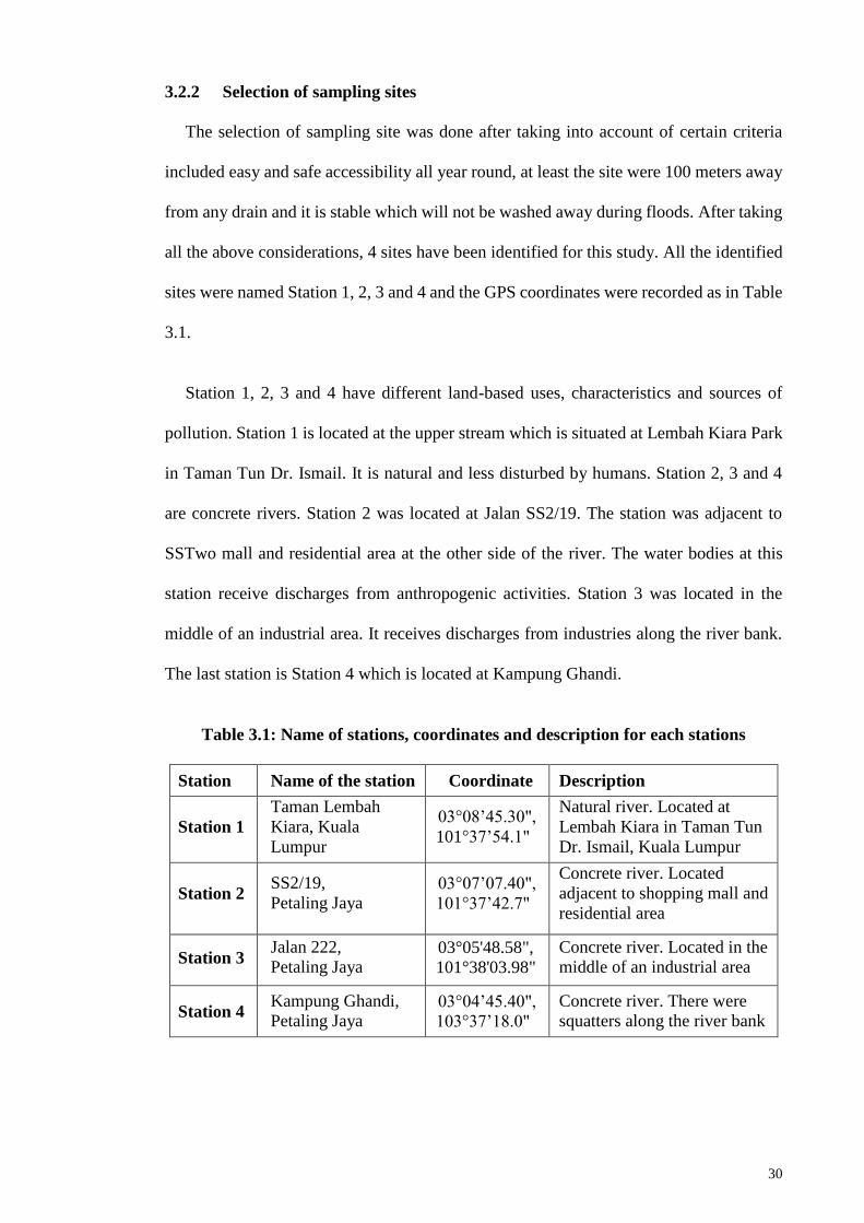
Table 3.1: Name of stations, coordinates and description for each stations ................... 30
Table 3.2: Sampling months and dates for data collection ............................................. 33
Table 3.3: Derivation of WQI (DOE, 2013) ................................................................... 35
Table 3.4: Guidelines on INWQs specification (DOE, 2011) ........................................ 36
Table 3.5: INWQs specification definitions (DOE, 2011) .............................................. 36
Table 4.1: Results of physico-chemical parameters for four sampling stations of Penchala
River ................................................................................................................................ 44
Table 4.2: Mean and standard deviation of physical characteristics for Station 1, 2, 3 and
4 of Penchala River ......................................................................................................... 50
Table 4.3: Abundance and distribution of macrobenthos at Station 1, 2, 3 and 4 of
Penchala River ................................................................................................................ 53
Table 4.4: Monthly results of richness, diversity and evenness index for the average of
four sampling stations of Penchala River........................................................................ 56
Table 4.5: Pearson’s correlation of coefficients (r) of physico-chemical parameters and
biotic indices of Penchala River ...................................................................................... 58
Table 5.1: Comparison results between previous and current study conducted at Penchala
River ................................................................................................................................ 63

xii
LIST OF SYMBOLS AND ABBREVIATIONS
1S1R : One State One River
APHA : American Public Health Association
BMWP : Biological Monitoring Working Party
BOD : Biological oxygen demand
COD : Chemical oxygen demand
CST : Communal septic tank
DID : Department of Irrigation and Drainage, Malaysia
DO : Dissolved oxygen
DOE : Department of Environmental, Malaysia
EPT : Ephemeroptera, Plecoptera and Tricoptera
INWQs : Interim National Water Quality Standards
IST : Individual septic tank
NGO : Non-government organisation
NH3-N : Ammonical nitrogen
NTU : Nephelometric Turbidity Units
PDC : Penang Development Corporation
TDS : Total dissolved solids
TSS : Total suspended solids
WQI : Water Quality Index

xiii
LIST OF APPENDICES
Appendix A: Raw data on WQI parameters of Penchala River………………… 95
Appendix B: Raw data on physical parameters of Penchala River…………….. 97

1
CHAPTER 1: INTRODUCTION
1.1 Background of study
1.1.1 Overview of urban river
‘Urban river’ is originally a natural river that flows through a heavily populated area.
The urban river expose to a wide range of anthropogenic pressures including pollution,
flow regime alterations, overfishing, habitat destruction and biological invasions. In
particular, many lowland regions concentrate agricultural and/or industrial activities
which adversely affect biological diversity in rivers (Compin, 2007). The impairment of
water quality at urban tropical river is mostly derived from the inflow of nutrients,
pesticides and heavy metals (Krueger, 1998; Beasley and Kneale, 2003; Schipper et al.,
2008).
Nowadays, urban tropical rivers are highly polluted due to impacts from tremendous
development and affected by human activities as well as urbanization. Urbanization of
the watershed increases impervious area thereby increases the intensity of runoff and peak
flow discharge rate. Other than that, it also increases the concentration of sediments and
nutrient loading and consequently alters the river morphology and flow patterns
(Bernhardt and Palmer, 2007).
Determination of the current water quality status of the urban tropical river is essential
to identify the pollutant which contaminate the rivers so that recovery action can be made
by the authority. Hence, preventive measures can be taken to avoid recurrence of the same
pollutant. All the preventive measures are necessary to preserve the river as it is a vital
resource in sustaining life, development and to the environment. In addition to that, the
river is very important as the main habitat for macrobenthos, fishes, amphibians and
others.

2
1.1.2 Application of macrobenthos as bioindicator
The terms of bioindicator refer to an organism that accumulates substances in their
tissue. This organism has the ability by giving response to the environmental level of
those substances or the extent (Hellawell, 1986). The biological indicator study involves
the identification of macrobenthos is a scientific analysis to determine the interactions
between macrobenthos with their surrounding environment. Aschengrau and Seage
(2007) defines ecological study as the examination of the relationship between exposure
and outcome by observing population level data rather than individual-level data. The
study had been focused on the comprehensive data for a population to review trends and
make interpretations of the river health condition or problem on a large scale. The
ecological study also involved study on diversity, distribution and calculation of biomass.
In addition, the study also takes into account the determination of the number of
organisms and competition between them as well as among ecosystem.
History of running water quality assessment based on biological indicators had been
developed in the 1980’s which about 60% is based on macroinvertebrate analysis (De
Pauw and Jawkes, 1994). Macrobenthos assemblages or guilds generally integrate
environmental changes in physical, chemicals and ecological characteristics of their
habitat over time space (Cook, 1976; Milbrink, 1983). In addition, macrobenthos have
thus been attractive targets of biological monitoring of environmental quality in aquatic
ecosystems in Europe and North America (Rosenberg and Resh, 1993). This new
development denotes that the natural structure and variability of invertebrate
communities. It derives biotic indices within a homogeneous physiographic ecoregion
could be surrounded by ordination, direct gradient analysis and canonical correspondence
analysis (Gauch, 1982; Ter Braak, 1986) and thereafter macroinvertebrate assemblages
or indices in suspected altered sites could be compared against those in reference sites.

3
1.2 Statement of problem
Malaysia has the highest dependency on the inland river system as a sources of clean
water for daily uses. Heavy industrialisation, rapid urbanisation and urban-expansion
make an increasement of pressure in finding the appropriate preservation and
conservation activities to sustain the river health. This situation give challenge to
researchers in order to discover alternative courses of action to improve water quality
(Muyibi et al., 2008).
In this study, the selected urban river is unique as the upstream is very clean which is
located at Kiara Park, Taman Tun Dr. Ismail. The river is use as a favourite recreational
spot for the local community of Taman Tun Dr. Ismail. Besides, it also supports a wide
range of biodiversity in and around its water. Moving to the downstream, 70 % of the
river has been channelized. The river is highly polluted with rubbish and sewage since it
was discharged by the residential area located along the river. In addition to that, the river
faces some continuous construction activities. The construction activities are being done
to maintain the stability of the riverbank while constructing a new structure across the
river. Thus, as a comparison between upstream to downstream, the water quality status at
the downstream deteriorates from Class I to Class IV.
The river also polluted with solid waste which were thrown from restaurants, wet
market and industrial discharge. As time goes by, the condition of the river worsens as it
becomes shallower and the flow of the water slower. The situation become more worsen
when it’s come to raining season. The natural flow of the river is now being stuck to let
river flushing off for its self-purification. This situation also gives negative impacts to the
aquatic ecosystem in the river. A clean river is known as an ideal place for aquatic species,
especially aquatic insects such as Odonata, Trichoptera, Coleoptera and Ephemeroptera
to breed. Now, it has been destroyed by the urbanization project along the river. Other

4
than that, the conversion flow of water from natural river into a concrete river prevents
its natural self-purification (Wang et al., 2012).
1.3 Aim and objectives
The aim of this study is to find an alternative way to determine water quality which is
cheap, rapid and economically cost effective. The determination of water quality by using
macrobenthos is expected to be one of the alternative way of assessing the current water
quality status. These alternative ways are important to manage urban river health. In an
urban city, a healthy river provides a panoramic scenery and further illustrates our
country, Malaysia as a beautiful country with beautiful rivers.
Government launched One State One River (1S1R) programme in 2005 to help the
Department of Irrigation and Drainage Malaysia (DID). The aim of this program is to
create awareness for the public about river restoration. River restoration is a process
where the degraded river being brought back to its normal condition. One State One River
promotes the involvement of local communities to participate in river management, in
order to create awareness for the citizens to keep our rivers clean and healthy (1S1R,
2016). Other than that, good management of urban river will able to control the discharge
of pollutants into the urban river. In Malaysia, the government has made a significant
effort to control the discharge of pollutants into a river by introducing Environmental
Quality Act 1974 (EQA, 1974). The act has listed various type of pollutants with its
permission limits which the offender will be convicted under one of its clause and/or be
fined as prescribed.
The development of squatters also can be controlled by using effective management
of the urban river. Suffian and Mohamad (2009) studied that the main factor that causes

5
a high number of squatters in Kuala Lumpur is economic status. The squatters affect the
water quality through their poor sewage system. Other than that a healthy urban river can
be used as a recreational spot. As mentioned earlier, the upstream of the selected river is
very clean. The local authorities can take this opportunity to build up the surrounding area
to a recreational area for a picnic, jogging and cycling.
Moving towards sustaining healthy urban river, this study was done to determine the
current water quality status and to study the effect of the deterioration of water quality
parameters to diversity and existence of macrobenthos at the selected urban river. At the
end of this study, multi-relationship among the parameters was established to see the
significant factor that affects the diversity and the existence of the macrobenthos. This
establishment serves as an alternative method to access the current water quality status
and river health instead of by relying solely on massive laboratory analysis. In addition,
this study could be the benchmark to evaluate future water quality changes.
To achieve the aim, this research was supported by three objectives and research
questions which are;
1. To determine physico-chemical parameter of Penchala River
2. To determine the distribution and abundance of macrobenthos of Penchala River
3. To determine the relationships between physico-chemical parameters and
biological indices of Penchala river
This study introduced a rapid determination of the current water quality status by
looking at the distribution and abundance of the macrobenthos. To validate the results,
the water quality derived from biological indicators were compared to the results obtained
from calculation of Water Quality Index (WQI).

6
1.4 Scope and limitation
This study covered the determination of water quality analysis that involves in the
calculation of WQI such as pH, dissolved oxygen (DO), chemical oxygen demand (COD),
biological oxygen demand (BOD), total suspended solid (TSS), and ammoniacal nitrogen
(NH3-N) as well as in-situ parameters such as temperature, conductivity and total
dissolved solids (TDS). This study also compared the basic physical parameters which
were water level, velocity and discharge. The sampling sites were limited to only four
stations since most of the river bank were inaccessible. The determination of
macrobenthos was limited to family level and it is a minimum requirement for calculation
of biotic index used in this study.
1.5 Implication by the limitation
The identification of macrobenthos was up to family level provide sufficient
information as the organic pollutant that can be detected clearly on family- based score
rather than species-score (Sandin and Hering, 2004). Lenat et al. (1994) recommend that
family level can be used since less taxonomy training is required to identify
macrobenthos. In addition, the time taken for sample identification can be shortened at
most of the macrobenthos can be identified to family level. Other than that, it is a
minimum requirement for calculation of biotic index used in this study. In addition, the
identification and classification at a family level also can prevent mistakes and
identification which leads to further data misinterpretation at the end of this study.

7
CHAPTER 2: LITERATURE REVIEW
2.1 River health for urban river
‘River health’ is define as highly depending on its usage. Every sector has their own
definition towards river health. For example, the river is considered healthy for
recreationist if they found the river can be swim, water skiing or boating. Rivers are also
considered healthy for drinking water utility as there is enough pure or purifiable water
throughout the year (Karr, 1999). Issues on maintaining the river health has become an
arisement important topic. Human activities that are involve changes in land use and
water resource development can alter physical, chemical and biological processes of river
ecosystem (Karr, 1991). Thus, the restoration and maintenance of healthy river ecosystem
have become important aim of river management (Gore, 1985; Karr, 1991; Rapport,
1991) as the river is believed can be restored (Gore, 1985; Brookes and Shields, 1996)
and also enhanced (Rapport, 1989).
Bunn and Arthington (2002) reported that river health in ecological concept is the
ability of the aquatic system to support and maintain key ecological processes and a
community or organisms with a species composition, diversity, and functional
organisation as comparable as possible to that undisturbed habitats within the region.
They also stressed that the ecologically healthy river will have flow regimes, water quality
and channel characteristics such that in the riparian zone, the majority of plant and animal
species are native and the presence of exotic species is not a significant threat to the
ecological integrity of the system. The native riparian vegetation communities are existed
to ensure the sustainability for the majority of the river’s length and native fish and other
fauna can freely move and migrate up and down the river. The most important

8
characteristic of the healthy river is major of the natural habitat features that are
represented and maintained over time (Postel and Richter, 2012)
‘Urban river’ is a river where a significant part of the contributing catchment consists
of development where the combined area of roofs, roads and paved surfaces results in an
impervious surface area characterising greater than 10% of the catchment (Beach, 2003;
Ladson, 2004).
Rivers are important as it provides the sources of clean water to Malaysian. Major
cities in Malaysia have been established and flourished along rivers. For example, the city
of Kuala Lumpur itself was started at the confluence of Klang and Gombak river (Keizrul,
2011 March 9). Moreover, the river also acts as an urban entity that has been played many
roles and contributes in many ways to urban development such as for transportation, water
supply, flood control, agriculture and power generation. Nowadays, urban river in
Malaysia has been polluted with rubbish, silt, sullage and domestic waste as it flew across
the highly urbanized area. As the time goes by, the river is now getting worse as it loses
their ability to make a self-purification (Wang et al., 2012).
Moving towards to the Vision 2020, Malaysia is facing a high demand of water and
it’s become a great pressure in preserving the current water resources as well as finding
alternative ways of action in order to improve water quality (Othman et. al., 2012). The
impairment of water quality is due to increasement of water demand from agriculture,
industry, hydroelectric generation and continued pollution. The consequences are further
exacerbated by population growth, rapid urbanization and climate changes (Birol et al.,
2006). Thus, rapid industrialization has been putting pressure on urban areas especially
in the Klang River Basin which is the densest populated area in the country.

9
In recent years, Malaysia has experienced water crisis at severe stage. For example,
the area of Klang Valley often had to deal with the water crisis due to decreasing of water
quality at Semenyih Dam perhaps polluted by a high concentration of ammonia. As a
consequence, the dam had to be closed for the water quality recovery process. The
awareness about importance of maintaining the water quality of river is being ignored by
most of the Malaysians. Rivers that formerly clean without any pollution is now at the
stage of growing concern (DOE, 2015).
Water pollution is generally generated from the point and non-point sources. The point
sources are discharges from industrial and sewage treatment plant and example of
pollution that generated from non-point are surface water runoff from agricultural land
use, housing area, commercialized area and industrial area. The development of squatters
along the river bank resulted in the river channel. This make the river bank to be used as
a convenient dump sites, waste from households, such as food scraps, plastics and sullage
whether in liquid or solid form has been thrown into the river without any sense of guilty.
Apart from that, the discharge waste with or without partial treatment from factories also
has been released indiscriminately into the river; thus reducing their drainage capacities
and, in the long run, creating an unsustainable environment (DOE, 2017 February 10).
2.1.1 Relationship between river health and urban river
The health level of the urban river is mostly affected by alteration of land use and
anthropogenic activities. The changes in the natural water flow caused by drought or
human intervention had created difficulty in living conditions for fish and other wildlife.
The level of health was disturbed as the water was overtaken for agricultural activities,
industry and conventional usage. In addition to that, the extreme agricultural activities
also cause fewer rainfall filters into the ground since it runs directly into the rivers instead
of flowing into drains and rivers. This situation will reduce the amount of water that is

10
recharged to groundwater system and further causing additional impacts to river
ecological health via decrease in the base flow of a system (Paul and Meyer, 2001).
Other than that, changes to the shape or structure of the river also can affect the river
health. This situation happened when there are barriers that prevents fish and other
creatures migrating naturally. The changes also remove all the plants from the riverbank
that further make it more likely to erode, reduces habitats for other wildlife, affects the
river’s natural temperature and reduces the soil’s ability to filter polluted water entering
the rivers (Tabacchi, 1998).
2.2 Threats to urban river
There are many factors that affected the urban river health, as listed below:
2.2.1 Channelisation
The rapid urbanisation forces all the engineers, scientist and environmentalist struggle
find the best tools to ensure the sustainability of the biodiversity and ecosystem. One of
the problems that faced by the urban river is channelisation. Channelisation is a practice
of dredging and straightening stream where finally it turned into artificial channels. This
practice is done to increase the flow rates and carrying capacities. Initially, this idea is to
make the river to flow straightly in order to prevent a flash flood, especially in the city.
The channel has now been extra-large and straight to allow it to take bigger flows that
would occur during severe rainfalls and could move away as much water as possible and
in a short period of time (McBride and Booth, 2005).
From the other side, channelisation affects the hydrology that gives significantly
influences to the water quality, temperature, nutrient cycling, oxygen availability and the
geomorphic processes that shape river channels and floodplains (Paul and Meyer, 2001).

11
Mahazar et al. (2013) reported that the urban river also can cause problems as it becomes
a mechanism for transporting plagues and diseases in certain countries as the
consequences of water blocked during flood event. Other than that, the alteration is a
natural regime that caused reducing or increasing of flows, altering seasonality of flows,
changing the frequency, duration, magnitude, timing, predictability and variability of
current events, altering surface and subsurface water levels and changing the pace of
rising or drop of water points. Even worse, the same report had recognised that the
alteration of natural flow regimes as a major factor contributing to the loss of biological
biodiversity and ecological function in an aquatic ecosystem. Because of that, a large
number of species, populations or ecological communities that rely on river flow for their
survival become threatened as extraction of water, which reduce the flowing of water that,
lead to a lower distribution of organic matter on invertebrate and vertebrates depend on
as well as this will kill vegetation depending on intermittent flooding, decreasing habitat
for invertebrate as a result. In addition, simplification of channel structure will result in a
dramatic decrease in the habitat value of the stream (Brooks et al. 2001). Other than that,
changes in physical, chemical and biological conditions of rivers as well as the
degradation of riparian zone increase the erosion thus leading to sedimentation impacts
upon aquatic communities (Bennett and Simon, 2004).
The above statement gives an idea that the chanellisation, alteration of natural flow
regimes and changes in physical, chemical and biological will affect the aquatic
organisms such as diatoms (Lowe and Pan, 1996; Hill et al., 2001) and macrobenthos
(Rosenberg and Resh, 1993; Metcalfe, 1989). Therefore, the aquatic organism has been
identified by many studies that they are suitable as a biological indicator to integrate their
total environment and their responses to complex sets of environmental conditions. Other
than that, biological indicator also offer the possibility to obtain an overview of the current
status of streams or rivers (Worf, 1980). In addition, many studies have proved that

12
macrobenthos can serve as biological indicators as can they can integrate their total
environment and their responses to complex sets of environmental conditions. Other than
that, they also can offer the possibility to obtain an ecological overview of the current
status of rivers (Rosenberg and Resh, 1993; Metcalfe, 1989; Soininen and Koinonen,
2004; Li and Liu, 2010; Lenat and Barbour, 1994; Statzner et al, 2001).
2.2.2 Extreme increasing and decreasing of water volume
Increasing and decreasing of water volume is depending on the quality of rain and the
ability of soil to store water (Berndtsson, 2010). Theoretically, when rain hits the surface
of soil which covered with grass, forested or other unpaved surfaces, the water soaks will
directly flow into the ground. As the water reach the ground, most of the water is absorbed
by roots and is stored in the soil. The water which is not absorbed or stored, will gradually
flows into streams and creeks. This make the stream to flow slowly and increases to a
peak flow, and later slowly decreases to a stable flow maintained by water stored in soils.
Consequence to the situation, when rain hits concrete, paved or other impervious surfaces
such as rooftops, sidewalks and driveways, the water immediately become runoff and
rapidly flows into the streams and rivers. This is because the water does not get a chance
to filter through the soil. As the water rises rapidly and this make a decrease of the size
of peak flow. Later, this situation also flushes fishes and insects. The worst situation that
can happen is when a large quantities of water flowing quickly through the stream
channels will cause the banks of the stream to erode, adding sediment to the stream and
further causing habitat loss. This situation will also drastically change the structure of the
stream bottom by washing out rocks, logs, and vegetation which all these structures
provide shelter and food for living animals in the stream (Finkenbine et al., 2000).

13
2.2.3 Shallow stream bottom
A healthy stream bottom generally made off from sediment, loose clay, gravels, logs,
loose sand and boulders. In addition, the natural streams have less erosion and sediment
deposition. Other than that, natural streams normally create flow patterns containing
numerous bends and usually inside the bends it contains finer substrate deposited, while
the outside of a bend tends to undercut the bank. This situation provides shallows in the
depositional area and pools in the erosional area. The urban river which undergoes
channelisation eliminates all of these processes and the habitat that they created.
Excessively increased flow and channelisation results in degradation or elimination of
natural substrate and thus decreased habitat diversity (Rapport and Whitford, 1999).
2.2.4 Loss of riparian vegetation
Another problem that the urban river faced is a loss of riparian vegetation. The riparian
vegetation is defined as an area of trees, shrubs and other plants located next to, and
upslope from, a body of water (Polyakov et al., 2005). The riparian vegetation plays an
important role specially to regulate water temperatures by shading off the stream. Losses
of these riparian vegetation had come to a results which is increasing of temperature This
phenomenon thus decrease the stream’s ability to hold oxygen. Moreover, riparian
vegetation also helps to filter pollutants and debris as well as stabilises stream banks by
reducing erosion and sediment transportation. In conjunction to that, riparian vegetation
also provide habitat for wildlife especially macrobenthos that live between their roots
2.2.5 Degradation of ecosystem services
The urban river also has to deal with degradation of ecosystem services. The
degradation of ecosystem services is happening directly or indirectly relates to severe
degradation of water cycle catchments and their reduced ability in managing water
resources based on environmental mechanisms such as physical and green water

14
retention, infiltration, interception and self-purification. The disruption has been
recognised by Wagner and Zalewski et al. (2009) that can be classified into four main
categories which are degradation of the hydrological process, disruption of the
biogeochemical cycles and physical degradation of aquatic habitats. The degradation of
the hydrological process is due to land use changes, water withdrawal from surface
ecosystem and groundwater, improper river channelization for flood control and land
drainage and soil erosion whereas the disruption of the biochemical cycles is affected by
increasing of diffuse nutrient export from degraded landscapes and condensed matter
outflow from urbanised areas.
Adaptation of hydro technical management or engineering is a potential to overcome
all of this disruption. The effectiveness of this method is highly depends on the climatic
conditions, the degree of natural processes degradation, cultural and social attitudes and
policy as well as financial mechanisms (Batrich et al., 2004).
2.3 Managing urban river
A healthy urban river should have a diverse and complex ecosystem for many
communities of plants and animals that exist together in balance. Chan (2012) stated that
the urbanization increased dramatically in all major cities and towns as the country
undergo rapid development for the last three or four decades. The expansion of agriculture
and industrialization activities greatly affected the water supply in terms of quantity and
quality (Chan, 2002).
The government has launched 1S1R program in 2005 to support the DID in order to
get full participation from stakeholders in organizing a river restoration and water quality
for the improvement program for one river in their state. One of the objectives is to ensure
15
cleanliness, living and valuable rivers with the minimum water quality of Class II (WQI
– 76.5 – 92.7) by 2015. As of 2013, Department of Environment Malaysia monitored 473
rivers all over Malaysia. In the percentages of, 58% (275) were asserted to be clean,
36.6% (173) were slightly polluted and another 5.3% (25) were found to be polluted
(DOE, 2013).
The urban river that was heavily been polluted is Klang River which located in the
Klang River basin, which is one of the densest populated areas of the country housing
that is consisting 3.6 million people (Chop et al., 2002). Due to the serious pollution, DID
has come out with a proposal to clean up the river and the objectives are; 1) to clean up
the Klang River and its major tributaries from rubbish and silt, 2) to improve the water
quality of the Klang River and its major tributaries to a standards minimum of Class III
standards and, 3) to beautify the riverine areas with a sceneric view to provide and
upgrade recreational facilities within the city. Other than that, the Federal Territory and
Klang Valley Development Division of the Prime Minister’s Department also take some
initiative to relocate about 2,650 squatters’ family which has been colonised along the
river bank. Unfortunately, the relocation process was unsuccessful due to the inability of
local authorities to provide alternative low-cost housing to the squatters (Chan, 1997).
Other than that, Sungai Penang also was listed as a polluted urban river by the Penang
State Local Government. The Sungai Penang used to be very clean but after sometimes
later the river has degraded too much and finally become one of the most polluted rivers
in Peninsular Malaysia. The pollution occurred because of lack in public participation.
The government also need to be well cooperate with non-government organization
(NGOs) in the country’s development and involving with NGOs in water conservation
and management since the role of NGOs is to link the industries and consumers (Chan,
2002).

16
Sungai Kluang is another polluted river. The river water of Sungai Kluang passes
through the residential areas of Bayan Baru, Bukit Gedong and Bayan Lepas Industrial
Zone before it drains into the Western Channel of Pulau Jerjak. Sungai Kluang is being
polluted while it is passing through the industrial zone. The pollution is caused by the
organic waste, suspended solids and heavy metals such as lead, nickel and zinc (Ibrahim,
2002). The NGOs, DID, Penang Development Corporation (PDC) united together with
the local residents to develop a riverside park that will cater for the recreation needs of
the Bayan Baru population. The programme provides a minimum landscaping, basic
recreational amenities and a cycle track of 4 km stretch that also provides a mechanism
for community participation in river management (Chan, 2002).
2.4 Water quality control for urban river
The water quality status of rivers in Malaysia has always been discussed by
government agencies, local authorities, NGOs, researchers and public at large. To access
the current status an extensive degree of quantification, the government is responsible to
make sure that all the rehabilitation measures and engineering control that involve with a
large cost to follow the appropriate plan and a very well decision making (Harding, 1998).
In Malaysia, the monitoring of river water quality has been started since 1978 by
Department of Environment Malaysia as the authority. Their primary role is to establish
a baseline and to detect water quality changes of a river and has been extended to
identifying of pollution sources as well. Recently, their efforts are considerable and had
been made in the past two decades to analyse pollution, either from point sources or non-
point source in several rivers. Point sources can be listed such as sullage discharge from
the residential area and partially treated effluent discharge from the industrial area. In
contrast, non-point sources are derived from diffused sources that do not have specific

17
discharge points such as from agricultural activities and surface run-off (DOE, 2017
February 10).
Referring to the report that was published by the Department of Environment Malaysia
(DOE) 2013, the major pollution comes from manufacturing industries, sewage treatment
plants, individual septic tank (IST), communal septic tank (CST), animal farm (pig
farming), agro-based industries, wet markets and food service establishments.
Evaluation of water quality status is being done by using Water Quality Index (WQI).
The WQI is a method that combines a group of water quality parameters in one concise
for a specific use (Davis and McCuen, 2005). WQI has been developed to assess the
suitability of water for a variety of uses and most of the WQI development in many
countries requires selection of water quality parameters and assigning optional weights
of the selected parameters.
The implementation of this method involves sampling of the river water at regular
intervals from designated stations for in-situ and laboratory analysis to determine its water
quality and biological characteristics. In the year of 2006, which is the latest, there are
891 manuals and 13 automatic monitoring stations (DOE, 2015) operated by Malaysia
which include Sabah and Sarawak. The automatic stations were installed at a sensitive
location, including upstream of water abstraction points. There are three types of
monitoring stations which are baseline, ambient and impact stations. The baseline station
was located at the upstream of the catchments or basin, which are located in the
undevelopment area or with minimum activities. The ambient station was located at the
downstream away from the either point or non-point sources to get the actual status of the
water quality. Different from others, the impact station was operated for the purpose of
enforcement. All the automatic stations have the ability to detect pollution influx at an
early stage.

18
DOE Malaysia (1994) had set up a guideline as a benchmark for river water to monitor
in Malaysia so that the quality of water is under control and not exceeding the limit that
could stress out the ecological inside. The guidelines were focused on water for domestic
water supply, fisheries and aquatic propagation, livestock drinking, recreation and
agricultural use which involves over 120 physio-chemical and biological parameters. The
WQI was used as a basis for assessment of a water body in relation to pollution load
categorization and comprises weighted linear aggregation of sub-indices of DO, BOD,
COD, NH3-N, TSS and pH.
After several studies were done, the department published an Interim National Water
Quality Standards (INWQs). The INWQs defined six classes, namely Class I, IIA, IIB,
III, IV and V which Class I indicate the ‘best’ while Class V indicate the ‘worst’.
The DOE had set up regulations to control pollutant loading from point and non-point
sources is the Environment Quality (Sewage and Industrial Effluent) Regulations 1979
which include two standards of effluent quality, Standard A and B. Standard A refers to
guidelines that need to meet by effluent discharged upstream of a water supply intake and
Standard B is for effluent that is discharged downstream. The aim of this regulation is to
support the development of water quality management approach for the long-term water
quality of the nation’s water resources.
2.4.1 Biological indicator for water quality monitoring
There are many ways to assess water quality in flowing water (lotic) and still water
such as lakes (lentic). The most common method is by assessing on water quality which
involves the determination of physical and chemical properties of the water. This method
is widely used around the world but they have generally failed to provide a consistent and
comprehensive condition of the water body. Other than that, physical measurement and
chemical analysis which are dependent to one another and ecological state is poorly

19
understood or too complex to understand. In addition, these methods are also do not take
into account important changes to river habitat and are frequently instantaneous
(Rosenberg and Resh, 1993).
The determination of water quality through physico-chemical characteristics only help
to identify sources of water contamination. Further analysis is needed to get information
on the health of the aquatic ecosystem. Hellawel (2012) concluded that the analysis of
physico-chemical characteristics only serves as a transient picture of ecosystem health
since concentration for each parameter will vary day to day and highly depending on the
time, discharges, precipitation and water flow patterns.
Matthews et al (1982), Rosenberg and Resh (1993) and Gibson et al. (1996) defined
monitoring water quality by using biological indicator is defined as an evaluation of the
condition of a water body using biological surveys and other direct measurements of the
resident biota in surface waters.
Compared to the biological indicator, the biological communities integrate all of the
environmental stresses whether caused by human or natural activities within unlimited
time. The success of this indicator can be qualified by the presence of sensitive species
of macrobenthos at a healthy river and the absence of them at a poor river. Beside
determination river health through physico-chemical method, biological communities in
rivers and streams are important components in the evaluation of water quality. Biological
communities provide an integrated and comprehensive assessment of the health over
time. It also gives an integrative measure of the overall health of the stream and
inadequately identifies impaired water (Karr, 1999).
The right selection of bioindicator is important since different types of bioindicators
have different tolerance towards certain concentration of pollutants. Hellawell (1986)

20
provide guidelines to select the best organism as indicators which were 1) readily
identified, 2) sampled easily and quantitatively, 3) wide distribution, 4) abundance
existence, 5) have economic importance, 6) readily accumulate pollutants and 7) have
low variability.
Macrobenthos consist of crustaceans, mollusks, insects and other visible invertebrates.
Plafkin et al (1989) mentioned that the macrobenthos are important bioindicator since
they inhabit the degraded or contaminated resources Other than that, the macrobenthos is
exposed directly to degradation throughout its life history. Resh (2008) studied that
macroinvertebrates provided the highest return for research fund spent. This statement
was supported by Bonada et al. (2006) who agreed that macrobenthos is accepted around
the world as biological monitoring of streams and rivers.
2.5 Introduction of macrobenthos as biological indicator to determine water
quality
Basically, macrobenthos are small animals without backbones that survive on and
under submerged rocks and gravel, logs, in the sediment, in between debris and aquatic
plants during their life cycle. Macrobenthos have special characteristics. Different species
have different tolerances to a variety of pollutants such as organic pollutants, sediments
and toxicants (William, 2005). Other than that, their variations also related to human
activity in water basins, such as urbanisation and agriculture (Fore and Grafe, 2002).
Macrobenthos is recognised to serve as good indicators for overall stream health as
they commonly inhabitants of streams. Rosenberg and Resh (1993), reported that the term
‘benthic’ means ‘bottom living’ and it is approved as these organisms usually inhabit at
the bottom of substrates for at least part of their life cycle. They play an important role in

21
the food webs, energy flow and in the circulation of nutrients as they serve as food for
other higher organisms such as fish (Rosenberg and Resh, 1993). The existence and
diversity of their population are highly dependent on the integration of the stream
conditions that occurred during their life cycles. Diversity such as water quality, habitat
characteristics, and changes in the flow, temperature and velocity. In addition,
macrobenthos also reacts to physical factors of ecological significance that include
streamflow, current velocity, channel shape, water depth, substrate and temperature and
water quality indicators such as the concentration of dissolved oxygen, salinity and pH.
Several publications have appeared in recent years documenting the potential of
macrobenthos as a biological indicator. Rosenberg and Resh (1993) stressed that the data
on physico-chemicals is very limited for determination of river health. The study was
supported by Oertal and Salanki (2003) who also agreed that the monitoring by using the
chemical approach alone is not realistic and not enough data can obtain as it is very
limited. In addition, they also argued that the approach would not take into account for
the additive, synergic or antagonistic effect that might occur and also lack important data
such trace metabolite and reaction products.
Turkmen and Kazanci (2010) have listed the advantages using macrobenthos as a
biological approach to monitoring water quality. From his study, macrobenthos served as
a better candidate compared to fish as they are high abundance and ubiquitous in nature.
In addition, macrobenthos also rich with families that responses to environmental changes
both natural and man-induced during their life cycle. Other than that, macrobenthos has
a sedentary lifestyle and long lifespan also give them advantages as pollutant indicator.
Furthermore, they are readily collected and identified and finally classified as sensitive.
Each of its families have a varied sensitivity of various types of pollutants. Their
presence and absence will reflect the health conditions of the river either healthy (clean)

22
or not healthy (polluted) (Karr, 1999). For example, the healthy river is favourable for
Trichoptera, Ephemeroptera and Plecoptera larvae whereas Diptera larvae are found
abundance in the not healthy river (Ab Hamid and Rawi, 2014). This characteristic might
useful in order to study and identify the synergistic effect of different type of pollutants
on a living organism (Cao et al., 1997). His study was parallel to Hellawell (1986) who
found that aquatic invertebrates respond to their variations in physical habitats.
2.5.1 Use of macrobenthos as water quality indicator
In Malaysia, various type of considerable effort has been made to achieve a
successfully analyse physical, chemical and biological pollution in several rivers.
However, there were only a few efforts that include the study on diversity and abundance
of macrobenthos for purposes of environmental bioassessment are available (Azrina,
2006). The study also mentioned that there is no comprehensive investigation on the
effect of the different pollution on the diversity of macroinvertebrate inhabiting
Malaysian’s river has been carried out.
A study on macrobenthos community structure and distribution in Sungai Pichong,
Gunung Chamah, Kelantan has been carried out by Aweng et al. (2012) to assess the
species and distribution of macrobenthos at the highland river and also determining the
physical and water quality factor that influence macrobenthos composition and
distribution. They stated that the distribution of macrobenthos is highly depended on
physical nature at the sub-stratum, nutritive content, degree of stability, oxygen content
and level of hydrogen sulphide which supported by Anbuchezhian et al. (2009).
Azrina et al. (2006) studied on the anthropogenic impacts on the distribution and
biodiversity of macrobenthos and water quality of the Langat River. They agreed that
anthropogenic activities affect the water quality, biodiversity and distribution of
macrobenthos. The macrobenthos with high in tolerance were present at all level of

23
pollution while macrobenthos which low level of tolerance will disappear at “poor”
Biological Monitoring Working Party (BMWP) score.
Other than that, biological monitoring was suggested to be used in recovery and
conservation effort. Chironomidae and Simuliidae have a high potential for detection of
organic pollutant while Hirudinea and Oligochaeta can be used for other polluted water
as experimentally measured by Weng and Chee (2015).
Wahizatul et al. (2011) studied that the diversity and abundance of aquatic insects and
values of biological indices in accessing water quality of Sungai Peres and Sungai Bubu
in Terengganu. The ratio of Ephemeroptera, Plecoptera and Tricoptera (EPT) to
Chironomidae is higher at the downstream stations in Sungai Peres and Sungai Bubu
shows the impacts of anthropogenic activities on the water quality, diversity and
distribution of aquatic insects were clear. This study agreed that biomonitoring approach
by using aquatic insect communities as bioindicator provide useful information for
appropriate management of freshwater streams in Malaysia.
2.5.2 Levels of tolerance of macrobenthos to water pollution
The tolerance value describes the resistance of organisms towards pollution. Numbers
are given to represent their tolerance or intolerance towards pollution. The tolerance
values for each family were developed by weighting species according to their relative
abundance. According to a study by Carter and Resh (2013), the tolerance value is
different based on their response to stressors such as an organic pollutant, toxic chemical
and heavy metals. The general pollution tolerance for common aquatic organism towards
the various level of dissolved oxygen is presented in Table 2.1.

24
Table 2.1: General pollution tolerance for common macrobenthos (Carter and
Resh, 2013)
Level of dissolved
oxygen
Level of tolerance
value
Groups of macrobenthos
High Low Caddisfly
Mayfly
Stonefly
Water Penny
Riffles beetle
Hellgrammite
Moderate Intermediate Damselfly
Horsefly
Crayfish
Cranefly
Dragonfly
Blackfly
Low High Mosquito
Aquatic earthworms
Moth fly
Rat-tailed maggot
Midget
Leech
2.5.3 Diversity indices
Diversity indices are a numerical expression that can provide a combination of
quantitative values of species diversity and qualitative information on the ecological
sensitivity of each taxon (Arslan et al. 2016). Graca (1998) defined biological indices as
numerical expressions coded according to the presence of biological indicators differing
in their sensitivity to environmental conditions. Gallardo et al., (2011) defined biotic
indices as numerical expressions that combine a qualitative measure of species diversity
with qualitative information on the ecological sensitivity of individual taxa. His definition
is based on two principles that are (1) macroinvertebrate Plecoptera, Ephemeroptera,
tricoptera, Gammarus, Asellus, red midges Chironomidae and Tubificidae disappear in
the order mentioned as the organic pollution level rises, and (2) the number of taxonomic
groups is reduced as pollution increases.

25
Accessing water quality by using biotic indices has been recognized as suitable criteria
for understanding the quality of the aquatic environment. Biotic indices for several
decades by many European researchers for routine rapid assessment of water quality in
rivers (Hering et al., 2010).
Biotic indices developed for a particular zone have been applied in other geographical
areas. For example, Belgian Biotic Index (De Pauw and Vanhooren, 1983) has been
developed for Belgium, applied in Portugal (Fontura and Moura, 1984), Indonesia
(Krystiano and Kusjantono, 1991) and Canada (Barton and Metcalfe Smith, 1992).
Biological Monitoring Working Party (BMWP) score system was initially developed for
river pollution surveys in the UK (Armitage, Moss, Wright and Furse, 1983) have been
successfully applied in Malaysia (Yap et al., 2003; Mahazar, 2013).
In 2005, water quality monitoring programmes in Poland were mainly based on the
determination of physical and chemical parameters. They intermittently used the saprobic
index which was based on the analysis of microorganisms that belong to plankton
community. By using plankton community, they were facing difficulties as many
limitations occur in the biological water-quality assessment such as the difficulties in the
taxonomic identification of microorganism and the lack of possibilities of the presentation
of local conditions. Therefore, interest has been shown in the application of biological
water quality monitoring techniques using macroinvertebrates which are advantageous,
cost effective and simple and later Poland had led to the adaptation of the BMWP score
system.
Mason (1980) stated that biotic indices have been developed to measure responses to
organic pollution and may be unsuitable for detecting other forms of pollution. Diversity
indices are used to measure stress in the environment. It has been seen large number
species are found in unpolluted environment, with no single species making up the

26
majority of the community and a maximum diversity is obtained when a large number of
species occur in relatively low number in a community. When an environment becomes
stressed, species sensitive to that particular stress tend to disappear. As result, species
richness will be reduced and the density of the surviving species will increase. Species
diversity indices usually take account of both the species richness and their evenness.
There are numbers of diversity indices but the most widely used is Shannon diversity
index, which is based on information theory (Sharma et al., 2010).

27
CHAPTER 3: METHODOLOGY
3.1 Introduction
This chapter present the sampling procedure that was used in this study. The aim of
the procedure is to get the adequate sample of the river water in Penchala River. The
samples should be small enough in volume to be transported conveniently and large
enough for analytical purpose. River water samples were collected from all four stations
to assess their current water quality by measuring their chemical and physical properties.
To achieve the research aim, a series of data sampling has been conducted from
November 2013 to October 2014. For each sampling date, the river water was sampled in
three replicates to ensure the accuracy.
3.2 Determination of location to represent urban river
Urban river refers to the river that flows through a well-developed area that covers
with dense population or industrial area (Walsh et al., 2005). The urban river is
contaminated by urban runoff which comes neither from a residential area, restaurants
nor industrial area. Historically, monitoring of physico-chemical studies at urban river
have been done by researchers in Klang Valley (Azrina et al., 2006; Chop et al., 2002,
Mahazar et al., 2014; Norhayati et al., 1997; Yap et al., 2003). The Penchala River was
chosen as an example to represent urban tropical river was because it can cover both
pristine and polluted river health conditions along its 14 km river body. The upper stream
was clean and natural with almost no disturbance from anthropogenic activities while the
lower part was in contrast. Other than that, Penchala River also received various sources
of pollutant neither from point sources nor non-point sources. In addition, Penchala River
can also provide a suitable context to examine on how the macrobenthos response to
deterioration of chemical and physical in space and time. As it flows through a highly

28
urbanized area of Kuala Lumpur and Petaling Jaya, it receives discharges from the
industrial, residential and squatter’s area make it become the best example of the urban
tropical river in Malaysia and perhaps it will be suitable to apply to other rivers for future
studies.
3.2.1 Background of Penchala River
Penchala River has 50 km2 of the catchment area. It is originally short, a clean river
which rich with aquatic biodiversity. Nowadays, the river body at Station 2, 3 and 4 has
been channelised for the drainage system and polluted by the domestic wastewater,
industrial wastewater, agricultural area and housing development along the river bank
The research was done along 14 km of Penchala River, starting from its upper stream
at Lembah Kiara Park and straight away to the downstream at Kampung Ghandi, right
before it meets Sungai Klang. Penchala River has 50km2 of the catchment area. It is
originally a short, clean river which is rich with aquatic biodiversity. The clean river has
been known as an ideal place for breeding for many aquatic species, especially aquatic
insects such as Odonata, Trichoptera, Coleoptera and Ephemeroptera (Voshell, 2005).
Nowadays, the river has been modified for the drainage system and polluted by the
domestic wastewater, industrial wastewater, agricultural area and housing development
along the river bank. From the same report, Department of Environment, Malaysia (DOE,
2013) also mentioned that the Penchala River has been polluted with rubbish, silt and
domestic waste as it flew across the highly urbanized area of Kuala Lumpur and Petaling
Jaya. Fathoni Usman et al. (2014) showed the trend of WQI from 1997 – 2007. The WQI
were decreased and slightly improved started from 2002 onwards ranging from Class V
– Class IV to Class IV – Class III as the 1 State 1 River programme was introduced by
the Selangor State’s Department of Irrigation and Drainage in 2002. Basically, the
programme was aimed to organise a river restoration and water quality improvement

29
programme with full stakeholder participation. However, a continuous monitoring and
activities to further improve the water quality is still needed.
Figure 3.1: Catchment of Penchala River (Mahazar et al., 2013)
30
3.2.2 Selection of sampling sites
The selection of sampling site was done after taking into account of certain criteria
included easy and safe accessibility all year round, at least the site were 100 meters away
from any drain and it is stable which will not be washed away during floods. After taking
all the above considerations, 4 sites have been identified for this study. All the identified
sites were named Station 1, 2, 3 and 4 and the GPS coordinates were recorded as in Table
3.1.
Station 1, 2, 3 and 4 have different land-based uses, characteristics and sources of
pollution. Station 1 is located at the upper stream which is situated at Lembah Kiara Park
in Taman Tun Dr. Ismail. It is natural and less disturbed by humans. Station 2, 3 and 4
are concrete rivers. Station 2 was located at Jalan SS2/19. The station was adjacent to
SSTwo mall and residential area at the other side of the river. The water bodies at this
station receive discharges from anthropogenic activities. Station 3 was located in the
middle of an industrial area. It receives discharges from industries along the river bank.
The last station is Station 4 which is located at Kampung Ghandi.
Table 3.1: Name of stations, coordinates and description for each stations
Station Name of the station Coordinate Description
Station 1
Taman Lembah
Kiara, Kuala
Lumpur
03°08’45.30",
101°37’54.1"
Natural river. Located at
Lembah Kiara in Taman Tun
Dr. Ismail, Kuala Lumpur
Station 2 SS2/19,
Petaling Jaya 03°07’07.40",
101°37’42.7"
Concrete river. Located
adjacent to shopping mall and
residential area
Station 3 Jalan 222,
Petaling Jaya 03°05'48.58",
101°38'03.98"
Concrete river. Located in the
middle of an industrial area
Station 4 Kampung Ghandi,
Petaling Jaya 03°04’45.40",
103°37’18.0"
Concrete river. There were
squatters along the river bank

31
Figure 3.2 to 3.5 shows the pictures of Station 1, 2, 3 and 4. From the figures, Station
1 is the only natural river compared to other stations which has been channelised as its
flow through the developed area.
Figure 3.2: Station 1
Figure 3.3: Station 2

32
Figure 3.4: Station 3
Figure 3.5: Station 4
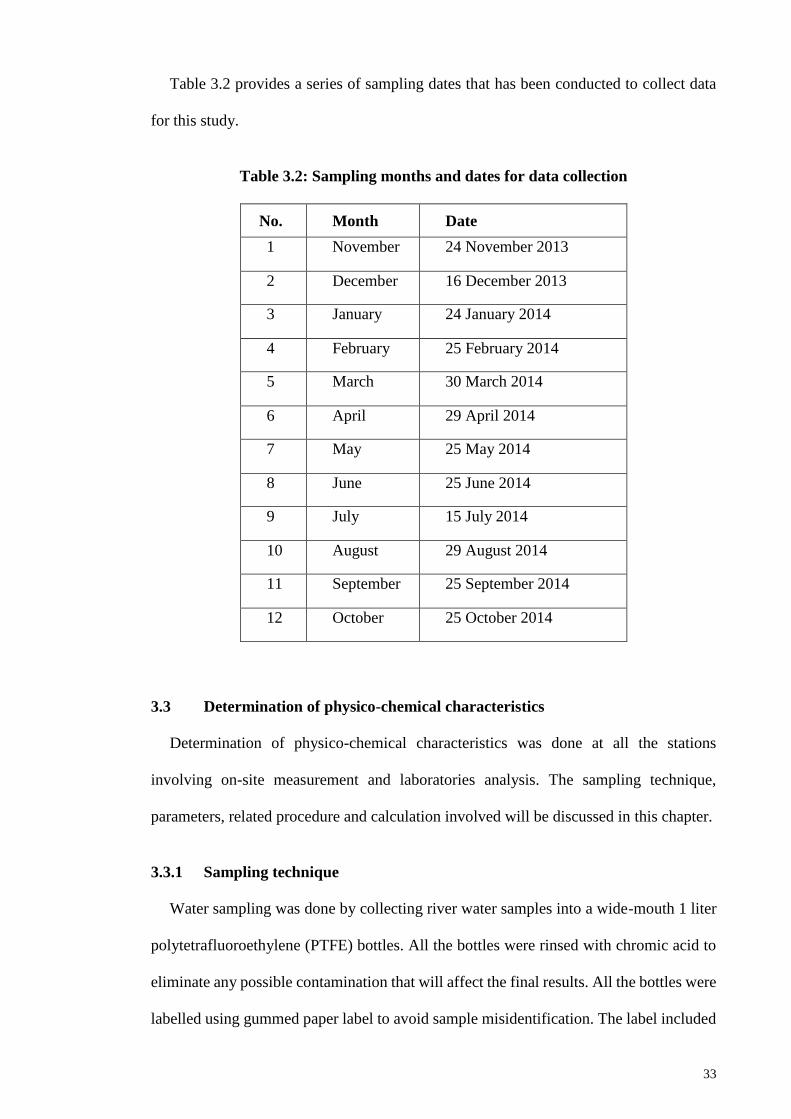
33
Table 3.2 provides a series of sampling dates that has been conducted to collect data
for this study.
Table 3.2: Sampling months and dates for data collection
No. Month Date
1 November 24 November 2013
2 December 16 December 2013
3 January 24 January 2014
4 February 25 February 2014
5 March 30 March 2014
6 April 29 April 2014
7 May 25 May 2014
8 June 25 June 2014
9 July 15 July 2014
10 August 29 August 2014
11 September 25 September 2014
12 October 25 October 2014
3.3 Determination of physico-chemical characteristics
Determination of physico-chemical characteristics was done at all the stations
involving on-site measurement and laboratories analysis. The sampling technique,
parameters, related procedure and calculation involved will be discussed in this chapter.
3.3.1 Sampling technique
Water sampling was done by collecting river water samples into a wide-mouth 1 liter
polytetrafluoroethylene (PTFE) bottles. All the bottles were rinsed with chromic acid to
eliminate any possible contamination that will affect the final results. All the bottles were
labelled using gummed paper label to avoid sample misidentification. The label included

34
the name of the station, date and time of collection. The samples were analysed for
chemical testing as soon as possible within 24 hours to avoid deterioration of original
characteristics. The water samples were kept in the ice box to maintain at 4oC prior to
transportation to laboratories for further analysis. Analysis of water quality was referred
to American Public Health Association (APHA, 2006), 21st edition as the main reference.
3.3.2 Water quality parameters
Water quality status was determined by conducting water analysis to the river water
samples. The analysis of water quality was done on-site and physical parameters of the
river can be accessed by conducting site monitoring, water sampling and on-site
measurement on water quality and physical parameters.
Water quality parameters such as temperature, conductivity, dissolved oxygen and pH
were measured in-situ. Dissolved oxygen (DO) was determined by using YSI DO meter
(YSI 550). Other parameters such as pH, conductivity and temperature were measured by
YSI meter (Multi-sensor) Model IQ Scientific. The Biological Oxygen Demand (BOD)
and Total Suspended Solids (TSS) were analysed in the laboratory by referring to APHA
standard method procedures (APHA, 2006). The COD were conducted by using HANNA
Instruments HI 93754B – 25 COD Reagent, Medium Range which covers results from 0
to 1,500 mg/L. Ammoniacal nitrogen (NH3-N) and Phosphate were analysed by using
Merck Spectroquant® Ammonium Test and Phosphate Test respectively by using the
photometric method.
A total of six water quality variables which were DO, BOD, COD, TSS, NH3-N and
pH were analysed to derive the water quality index of the Penchala River. The
calculations were done by using their sub- indices named SIDO, SIBOD, SICOD, SIAN, SISS
and SIpH. Finally, the WQI was calculated by using equation of Malaysian Department of
Environment (DOE) (2011) as follows;

35
𝑊𝑄𝐼 = (0.22 × 𝑆𝐼𝐷𝑂) + (0.19 × 𝑆𝐼𝐵𝑂𝐷) + (0.16 × 𝑆𝐼𝐶𝑂𝐷) +
(0.15 × 𝑆𝐼𝐴𝑁) + (0.16 × 𝑆𝐼𝑆𝑆) + (0.12 × 𝑆𝐼𝑝𝐻) Eq. 3.1
where, WQI = water quality index; SIDO = sub-index of DO; SIBOD = sub-index of BOD;
SICOD = sub-index of COD; SIAN= sub-index of AN; SISS = sub-index of TSS; SIpH= sub-
index of pH. The sub-index of the respective water quality parameters is calculated
according to the best fit equations as in Table 3.3.
Table 3.3: Derivation of WQI (DOE, 2013)
Sub-index for DO (in % saturation)
SIDO = 0 for x ≤8
= 100 for x ≤92
= -0.395 + 0.030x2 - 0.00020x3 for 8 < x < 92
Sub-index for BOD
SIBOD = 100.4 - 4.23x for x ≤ 5
= 108* exp(-0.055x) - 0.1x for x > 5
Sub-index for COD
SICOD = -1.33x + 99.1 for x ≤ 20
= 103* exp(-0.0157x) - 0.04x for x > 20
Sub-index for NH3-N
SIAN = 100.5 - 105x for x ≤ 0.3
= 94* exp(-0.573x) - 5* I x - 2 I for 0.3 < x < 4
= 0 for x ≥ 4
Sub-index for SS
SISS = 97.5* exp(-0.00676x) + 0.05x for x ≤ 100
= 71* exp(-0.0061x) + 0.015x for 100 < x < 1000
= 0 for x ≥ 1000
Sub-index for pH
SlpH = 17.02 - 17.2x + 5.02x2 for x < 5.5
= -242 + 95.5x - 6.67x2 for 5.5 ≤ x < 7
= -181 + 82.4x - 6.05x2 for 7 ≤ x < 8.75
= 536 - 77.0x + 2.76x2 for x ≥ 8.75

36
The respective class designation for the WQI scores, in turn, is tabulated in the Table
3.4:
Table 3.4: Guidelines on INWQs specification (DOE, 2011)
Parameters
Unit
Classes
I II III IV V
Ammoniacal
nitrogen
mg/l <0.1 0.1 – 0.3 0.3 – 0.9 0.9 – 2.7 >2.7
BOD mg/l <1 1 – 3 3 – 6 6 – 12 >12
COD mg/l <10 10 – 25 25 – 50 50 – 100 >100
DO mg/l <7 5 – 7 3 – 5 1 – 3 <1
pH mg/l >7 6 – 7 5 – 6 <5 >5
TSS mg/l <25 25 – 50 50 – 150 150 – 300 >300
WQI mg/l >92.7 76.5 – 92.7 51.9 – 76.5 31.0 – 51.9 <31.0
Table 3.5 provides definition on the class identified. From the Table 3.5, rivers which
fall under Class I, IIA, IIB and III are suitable for water supply while Class V river is
prohibited for water supply and also for irrigation. Other than that, Table 3.5 also provides
information on the specification of each river class. Class I – III rivers specify the water
quality level necessary to sustain macro aquatic life, with varying degree of sensitivity.
Class IV can be used for irrigation whereas Class V is considered to have minimal
beneficial usage.
Table 3.5: INWQs specification definitions (DOE, 2011)
Class Definition
I
Conservation of natural environment Water supply I – Practically no treatment necessary (except
by disinfection or boiling only)
Fishery I – Very sensitive aquatic species
IIA Water supply II – Conventional treatment required
Fishery II – Sensitive aquatic species
IIB Recreational use with body contact
III
Water supply III – Extensive treatment required Fishery III – Common of economic value, and tolerant
species, livestock drinking
IV Irrigation
V None of the above

37
3.3.3 Physical characteristics
Physical parameters of the river were divided into two parameters which are
measurement of velocity and calculation of discharge.
Velocity (V)
The stream velocity for all the stations was measured by identifying the best spot which
is straight, free from large objects with noticeable current with a depth as uniform as
possible were selected. For this study, the current meter of propeller type was used to get
the stream flow. The propeller was placed in about 2 cm from the water surface. Then it
was let to move freely for 30 seconds. The current meter converted the velocity into a
count of rotations. Then finally, the count was calculated to get the actual stream flow
reading (Hauer and Lamberti, 2011).
𝑉𝑒𝑙𝑜𝑐𝑖𝑡𝑦, 𝑉 = 0.1025 𝑁 + 0.028 Eq. 3.2
In the case of too low velocity at Station 4, the traditional method was adopted. The
traditional method was used floating polystyrene to travel at a known length and noting
its position in the river. The floating polystyrene was moved with the same velocity as
the surface of the water (Hauer and Lamberti, 2011). The calculations involved were;
𝑉𝑒𝑙𝑜𝑐𝑖𝑡𝑦, 𝑉 =𝑡ℎ𝑒 𝑑𝑖𝑠𝑡𝑎𝑛𝑐𝑒 𝑜𝑓 𝑓𝑙𝑜𝑎𝑡 𝑝𝑜𝑙𝑦𝑠𝑡𝑦𝑟𝑒𝑛𝑒 𝑡𝑟𝑎𝑣𝑒𝑙𝑙𝑒𝑑 (𝑚)
𝑡𝑖𝑚𝑒 Eq. 3.3
River water discharges (Q)
The stream discharges were calculated by the following equation (Hauer and Lamberti,
2011);
𝐷𝑖𝑠𝑐ℎ𝑎𝑟𝑔𝑒𝑠, 𝑄 = 𝐴𝑟𝑒𝑎 × 𝑉𝑒𝑙𝑜𝑐𝑖𝑡𝑦 Eq. 3.4

38
Calculation of area involves measurement of water depth and river width. The water
level was measured by using staff gauge by placing the gauge into the river until it reaches
the bottom. The river width was measured by using a measuring tape (Hauer and
Lamberti, 2011). The ‘0’ point should be anchored at the wetted edge of the stream. The
end of the tape was anchored at the opposite wetted edge. Thus, after the measurement of
water level and river width were collected, the data were calculated by using the equation
above, with results of velocity which had calculated earlier. Measurement of river width
were constant through this study as Penchala River is a concrete river.
3.4 Sampling of macrobenthos
A sampling of macrobenthos involved site selection for sampling, methods for
sampling, laboratory analysis, identification and calculating the biotic index to determine
its species richness and species diversity.
3.4.1 Site selection for sampling macrobenthos
The selection of sampling location is very important. The failure to identify the best
location to collect the benthic will lead to inaccurate data. The location should be at least
100 m upstream from any road or bridge crossing to minimize its effect on stream
velocity, depth and overall habitat quality. Other than that, the suitability also ensures that
there is no major tributaries discharge to the stream nearby (Hauer and Lamberti, 2011).
3.4.2 Method for sampling macrobenthos
The macrobenthos was collected on every sampling dates from November 2013 to
October 2014 by using 0.3m x 0.3m Surber sampler. Samples were taken in duplicates at
each station. The Surber sampler was placed face upstream, to allow the current to push
the sample into the net. The upstream were disturbed for three minutes using the heel of

39
the boot, dislodge the upper layer of cobble or gravel and scrape the underlying bed.
Larger substrate particles were picked up and rubbed by hand to remove attached
organisms. All the samples were transferred from the net to nylon sealed bag and were
preserved with 70% ethanol for further analysis in the laboratory (Hauer and Lamberti,
2011).
3.4.3 Identification of macrobenthos
In the laboratory, the sample was rinsed in a 500 µm mesh sieve to remove alcohol
and fine sediment then was placed into a shallow white pan and a small amount of water
were added to facilitate sorting. All the sorted organism was placed into labelled
containers and preserved in 70% ethanol.
The macrobenthos were identified to the family level. They were identified by
comparing collected specimens with illustrations of the groups as well as by using
identification keys. Keys used in this study were referred to Merrit and Cumins (1996)
and Mc Cafferty (1981). From the guidebook, keys generally consist of a series of paired
descriptions of particular bodily features such as wings and legs. The keys were numbered
and the best description that fit the specimen was chosen. After all the specimens were
identified to family level, the biotic score was calculated accordingly.
3.5 Measurement of biological indices
The biological indices used in this study were as follows:
3.5.1 Shannon-Weiner Diversity Index
Shannon-Weiner Diversity Index is a fast and reliable tool to identify major changes
in community structure of macrobenthos species (Pettersson, 1997). The Shannon-
Weiner Diversity Index was calculated in the following way:

40
𝐻′ = − ∑ 𝑝𝑖 ln 𝑝𝑖 Eq. 3.5
Where ‘pi’ is the proportion of individual macrobenthos in order i. The ‘pi’ also can be
calculated as pi = ni/N, where ni is the number of individual in order and N is the total
numbers of individual in the community.
3.5.2 Simpson Diversity Index
Simpson’s Diversity index shows the relative of rare species or common species in a
community (Mandaville, 2002). It has ranged from 0 – 1, which 0 indicates high level of
diversity. It was calculated as:
𝐷 = 1 − Σ 𝑛 (𝑛−1)
𝑁 (𝑁−1) ………………………………………………………Eq. 3.6
where n is the total number of macrobenthos of a particular order and N is the total number
of macrobenthos of all orders. D is a measure of dominance, thus as D increases, the
diversity of macrobenthos decreases.
3.5.3 Margalef Richness Index
Margalef Richness Index is the simplest measure of biodiversity and is simple count
the number of different species in the study area (Gamito, 2010). It is used to get species
richness which standardises the number of species encountered against the total number
of individuals encountered. The Margalef richness index can be calculated as:
𝐷𝑀𝑔 =(𝑠−1)
ln 𝑁 Eq. 3.7
where s is the number of species recorded and N is the total number of individuals in the
sample.

41
3.5.4 Pielou Evenness Index
Species evenness is calculated to monitor how close in numbers each species in an
area are. In this study, the evenness is represented by Pielou’s Evenness index (Pielou,
1966) which can be calculated equation below:
𝐽 =𝐻′
ln(𝑆) Eq. 3.8
where H’ is the Shannon – Weiner diversity index and S is a total number of observed
species in the community. The index can have values ranging from 0 – 1 where if there
are frequent variations in the community, the index will have higher values.
3.6 Statistical Analysis
In this study, Pearson correlation coefficient (r) among the six water quality
parameters in WQI formula were performed by using IBM SPSS Statistics version 22 to
find degree of significance relationship among the parameters. Other than that, correlation
coefficient between WQI values and parameters against biological indices was performed
to investigate the effects of WQI value and parameters to richness, diversity and evenness
index of macrobenthos at Penchala River. Statistical significance was tested at the alpha
level of 0.05 and 0.01 with 95% and 99% confidence level, respectively.

42

43
CHAPTER 4: RESULTS
This chapter presents results on physico-chemical parameters and collection of
macrobenthos from November 2013 to October 2014 at four selected stations along
Penchala River. As mentioned in Chapter 3, water sampling for determination of physico-
chemical characteristics and collection of macrobenthos has been done at the same point
of sampling to ensure all the results can be correlated at the end of this study.
4.1 Physico-chemical characteristics at Penchala River
Physico-chemical characteristics were determined monthly in the period of the one-
year interval which was from November 2013 to October 2014.
4.1.1 Chemical characteristics at Penchala River
Figure 4.1: Monthly results of Water Quality Index (WQI) for the average
of four sampling stations of Penchala River
Figure 4.1 shows the monthly WQI of the four stations of Penchala River from
November 2013 to October 2014. According to NWQS, the WQI values of the Penchala
River from November 2014 to October 2014 were classified under Class III, where the
Class III
Class IV
Class II

44
water requires extensive treatment for water supply purposes, being suitable only for very
tolerant and for livestock drinking.
The highest WQI value of 71.0 was recorded in November 2013 and the lowest WQI
value of 58.1 was recorded in February 2014. Starting November 2013 to February 2014,
the WQI value was degraded from 71.0 to 58.1. The WQI value was improved to 58.7 in
March 2014 and further increased to 60.0 in April 2014. However, the value was slightly
decreased to 59.1 in May 2014. The value started to recover to 63.6 in June 2014 and 65.0
in July 2014. Again, the value was dropped in August 2014 where the WQI value of 58.6
was recorded and increased to 61.6 in September 2014 and 60.0 in October 2014. The
range, mean and standards deviation for physico-chemical parameters were summarised
in Table 4.1.
Table 4.1: Results of physico-chemical parameters for four sampling stations of
Penchala River
Parameter Range Mean ± S.D Water quality
class
Temperature (℃) 26.5 – 28.7 28.0 ± 0.60
pH 5.6 – 7.0 6.0 ± 0.47 II
DO (mg/l) 2.1 – 3.7 2.9 ± 0.48 IV
COD (mg/l) 22 – 58 34 ± 12.19 III
BOD (mg/l) 4 – 15 9 ± 3.41 IV
TSS (mg/l) 7 – 23 16 ± 5.82 I
NH3-N (mg/l) 0.3 – 3.8 1.6 ± 1.18 IV
Phosphate (mg/l) 0.4 – 1.3 0.8 ± 0.25
WQI 58.1 – 71.0 62.4 ± 4.16 III
Table 4.1 shows the results of physico-chemical parameters with its class according to
DOE water quality classification for four sampling stations of Penchala River. The table
shows variation of classification where TSS were classified under Class I, pH were
classified under Class II, COD was classified under Class III and DO, BOD and NH3-N

45
were classified under Class IV. Overall, the WQI were classified under Class II according
to DOE water quality index classification (DOE, 1994). Below are the individual results
for all the parameters by months.
Dissolved Oxygen (DO)
Figure 4.2: Monthly results of DO for the average of four sampling stations of
Penchala River
Figure 4.2 shows the monthly results for dissolved oxygen for the average of four
sampling stations of Penchala River. DO is a measure of the quantity of oxygen gas freely
available in water. The concentration of DO is very important to aquatic life such as
macrobenthos. The concentration of DO in an unpolluted fresh water will be close to 10
mg/L and concentration less than 2 mg/L will kill the aquatic life.
From Figure 4.2, the results were distributed under Class III and IV. The concentration
of DO were at 3.44 mg/L at the beginning of the study. The concentration was decreased
to 3.11 mg/L and 2.97 mg/L in December 2013 and January 2014, respectively. The
concentration was further decreased to 2.42 mg/L in February 2014. The results were rose
up to 2.88 mg/L in March 2014. In April and May 2014, the DO level back to Class III
with result of 3.66 mg/L and 3.38 mg/L, respectively. The concentration DO fell to the
Class II
Class III
Class IV

46
lowest in June 2014 with only 2.14 mg/L was recorded. Starting July 2014, the results
remain relatively stable with 2.74 mg/L in July 2014, 2.51 mg/L in August 2014, 2.60
mg/L in September and 2.36 mg/L was recorded in October 2014.
Biological oxygen demand (BOD) and chemical oxygen demand (COD)
Figure 4.3: Monthly results of BOD and COD for the average of four sampling
stations of Penchala River
Figure 4.3 shows monthly results for biological oxygen demand and chemical oxygen
demand for the average of four sampling stations of Penchala River. The BOD of the
Penchala River were categorised under Class IV and Class III for COD (Table 4.1).
BOD refer to the amount of oxygen required to decompose organic matter in a unit
volume of water while COD is a measure of the capacity of water to consume oxygen
during the decomposition of organic matter and the oxidation of inorganic chemicals such
as ammonia and nitrite. Thus, concentration of COD is always greater than concentration
of BOD as COD does not differentiate between biologically available and inert organic
matter.

47
From Figure 4.3, the results of BOD were distributed under Class III, IV and once
under Class V in March 2014. The results were in the range of 4 – 5 mg/L with average
of 9 ± 3.41 mg/L. The results were stabilised in Class III from November 2013 to February
2014 and were suddenly rose up to Class V with result of 15 mg/L in March 2014. Started
from April 2014, the results remain relatively stable in Class IV until October 2014.
The monthly COD concentration in the Penchala River for the period from November
2013 to October 2014 are presented in Figure 4.3. The concentration of COD were in the
range of 22 – 58 mg/L with average of 34±12.19 mg/L. The results were scattered in Class
II and III from November 2013 until July 2014 and suddenly rose up to 58 mg/L which
classified in Class IV in August 2014. After that, the results were back to Class III with
38 mg/L was recorded in August 2014 and degraded to Class IV in October 2014.
pH
Figure 4.4: Monthly results of pH for the average of four sampling stations of
Penchala River
Figure 4.4 shows monthly results for biological oxygen demand and chemical oxygen
demand for the average of four sampling stations of Penchala River. In general, the pH

48
for water should be at 7 which is neutral. pH value less than 7 indicate the water is acidic
with corrosive properties and pH value more than 7 indicate alkaline properties (Ching et
al., 2015). pH is very important water quality parameter as most of the aquatic life is very
sensitive to pH variations especially when the pH is altered outside their tolerance limits
(Courtney and Claments, 1998). From Figure 4.4, the pH values were in the range of 5.6
to 7.0 which was scattered in Class II and III. Overall, there were no significant changes
in pH during the study period.
Ammoniacal nitrogen (NH3-N)
Figure 4.5: Monthly results of NH3-N for the average of four sampling stations
of Penchala River
Figure 4.5 shows monthly results for ammonical nitrogen for the average of four
sampling stations of Penchala River. At the beginning of the study, the concentration of
NH3-N were classified under Class IV and Class III in January 2014. The concentration
of NH3-N was degraded to Class V with result of 2.83 mg/L was recorded in February
2014. The level of NH3-N in March 2014 was recovered to 1.90 mg/L and suddenly the
result boost up to the peak where 3.83 mg/L of NH3-N was recorded in April 2014. In
Class V
Class IV
Class III

49
May 2014, the level was improved to 2.93 mg/L and further improved to 0.27 mg/L in
June 2014. There were no significant changes in July 2014 and August 2014 but the level
was started to degrade again in September 2014 and October 2014.
Total suspended solid
Figure 4.6: Monthly results of TSS for the average of four sampling stations of
Penchala River
Figure 4.6 shows monthly results for total suspended solid (TSS) for the average of
four sampling stations of Penchala River. The TSS is the solid matter in a water that can
retained on a glass fiber filter with a pore size less than 2 µm. It is typically consisting of
fragmental minerals, silt, plankton, sand, nutrients and metal that have attached to water
particles (Ching et al., 2015). From figure 4.6, the graph shows that the concentration of
TSS in Penchala River were scattered in the range of 7 – 23 mg/L and it is classified under
Class I. The highest level of TSS was recorded in September 2014 and June 2014 was
recorded to have the lowest level of TSS.

50
4.1.2 Physical characteristics at Penchala River
Results for water level, velocity and water discharge for Station 1, 2, 3 and 4 from
November 2013 to October 2014 which has been summarised into mean and standards
deviation in Table 4.2.
Table 4.2: Mean and standard deviation of physical characteristics for Station 1,
2, 3 and 4 of Penchala River
Parameter Station 1 Station 2 Station 3 Station 4
Water Level (m) 0.17±0.16 0.39±0.12 0.38±0.06 0.77±0.61
Velocity (m/s) 0.296±0.122 0.452±0.497 0.324±0.094 0.471±0.554
Discharge (m3/s) 0.083±0.120 2.784±3.539 1.661±0.732 6.908±7.248
Area (m2) 0.44±0.71 5.58±1.69 4.94±0.83 19.27±15.23
Width (m) 1.80±2.08 14.3 13 25
From Table 4.2, the water level of Penchala River ranged from 0.17 m to 0.77 m where
the deepest area was measured at Station 4 (0.77 m) and the shallowest area was measured
at Station 1 (0.17 m).
Water level
Figure 4.7: Monthly results of water level for the average of four sampling
stations of Penchala River

51
Figure 4.7 shows the monthly results of water level for the average of four sampling
stations of Penchala River. From the figure, the water level for every stations were
remained relatively stable with no significance changes through the sampling activities.
However, results recorded for Station 1 for June 2014 and Station 4 for January and
February 2014 shows that the water level has been disturbed which cause the results were
rose up to the maximum.
Velocity
Figure 4.8: Monthly results of velocity for the average of four sampling stations
of Penchala River
Figure 4.8 shows the monthly results of river velocity at Station 1, 2, 3 and 4 of
Penchala River. From the figure, the river velocity for every stations were remained
relatively stable with no significance changes through the sampling activities. The
significant changes of the results only occur in September and October 2014.

52
Discharge
Figure 4.9: Monthly results of discharge for the average of four sampling
stations of Penchala River
Figure 4.9 shows the monthly results of water discharge at Station 1, 2, 3 and 4 of
Penchala River. From the figure, the water discharge for every stations were remained
relatively stable with no significance changes through the sampling activities. The
significant changes of the results only occur in September and October 2014.
4.2 Abundance and distribution of macrobenthos at Penchala River
A total of 1043 individual of macrobenthos were found at Station 1, 2, 3 and 4. From
the number, 465 (44%) was collected at Station 1, 176 (17%) at Station 2, 372 (36%) at
Station 3 and another 30 (3%) individual was found at Station 4 which presented in Table
4.3. All the collected macrobenthos were belong to 9 orders which were Ephemeroptera,
Plecoptera, Trichoptera, Odonata, Decapoda, Coleoptera, Diptera, Basommatophora and
Hirudinida.

53
Table 4.3: Abundance and distribution of macrobenthos at Station 1, 2, 3 and 4
of Penchala River
Order Family Station
1
Station
2
Station
3
Station
4 Total
Tricoptera Hydropsychidae 94 - - - 94
Philopotamidae 18 - - - 18
Hydroptilidae 1 - - - 1
Ephemeroptera Baetidae 22 - - - 22
Heptageniidae 14 - - - 14
Plecoptera Capniidae 14 - - - 14
Peltoperlidae 9 - - - 9
Perlidae 2 - - - 2
Odonata Coenagrionidae 46 - - - 46
Calopterygidae 4 - - - 4
Aeshnidae 1 - - - 1
Gomphidae 1 - - - 1
Diptera Chironomidae 38 131 181 - 350
Simuliidae 18 - - - 18
Tipulidae 21 - 5 - 26
Ceratopogonidae 1 - - - 1
Coleoptera Elmidae 14 - - - 14
Decapoda Potamidae 54 - - - 54 Aatyidae 49 - - - 49
Palaemonidae 29 - - - 29
Basommatophora Physidae 9 29 79 28 145
Lymnaeidae 4 - 3 - 7
Planorbidae - 16 54 - 70
Thiaridae 2 - 8 2 12
Oligochaeta Lumbricidae - - 40 - 40
Hirudinida Hirudinidae - - 2 - 2
No. of individuals
(N)
465 176 372 30 1043
No of family (S) 23 3 8 2
Percentage (%) 44 17 36 3
Table 4.3 also shows the number of macrobenthos according to their family with its
percentage. There were 26 families were found which belongs to 8 orders. From the
results in Table 4.3, there were a high percentage of Trichoptera (Hydropsychidae;

54
20.2%) existed at Station 1. The percentage were followed by Decapoda (Potamidae;
11.6%), Decapoda (Atyidae; 10.5%) and Odonata (Coenagrionid; 9.9%). Other than that,
it was found that Diptera (Chironomidae; 8.2%), Diptera (Palaemonidae; 6.2%),
Ephemeroptera (Baetidae; 4.7%), Diptera (Simuliidae; 3.9%), Diptera (Tipulidae; 4.5%)
Trichoptera (Philopotamidae; 3.9%), Plecoptera (Capniidae; 3.0%), Coleoptera (Elmidae;
3.0%), Ephemeroptera (Heptageniidae; 3.0%) and Plecoptera (Peltoperlidae; 1.9%) also
were found at this station. In addition, the presence of some other macrobenthos which
were less than 1 percentage were Odonata (Lymnaeidae; 0.9%), Odonata
(Calopterygidae; 0.9%), Odonata (Aeshnidae; 0.2%), Odonata (Gomphidae; 0.2%),
Trichoptera (Hydroptilidae; 0.2%), Diptera (Ceratopogonidae; 0.2%) and
Basommatophora (Thiaridae; 0.4%).
The existence of macrobenthos at Station 2 has been shown in Table 4.3. From the
table, there were only two families existed at Station 2, which were Diptera with 74.4%
and Basommatophora with 25.6%. The only Dipteran existed at this station was
Chironomidae (74.4%) while there were two families of Basommatophora existed which
were Physidae (16.5%) and Planorbidae (9.1%).
Station 3 consist of Diptera (50.0%), Basommatophora (38.7%), Oligochaeta (10.8%)
and Hirudinea (0.5%). When the order is breakdown into family level, the highest
percentages of macrobenthos present at Station 3 was Chironomidae which was 48.7%
followed by Physidae (21.2%), Planorbidae (14.5%), Lumbricida (10.8%), Thiaridae
(2.2%), Hirunida (0.5%) and Lymnaeida (0.8%). There were only Physidae (93.3%) and
Thiaridae (6.7%) existed at Station 4.

55
Figure 4.10: Abundance of macrobenthos at Station 1, 2, 3 and 4 from
November 2013 to October 2014 of Penchala River
Figure 4.10 shows the abundance and distribution of macrobenthos collected at Station
1, 2, 3 and 4 from November 2013 and October 2014. From the figure, there were high
numbers of macrobenthos presented in December 2013 to March 2014. The numbers were
reduced in average of 42 to 58 in April to July 2014.
Figure 4.11: Percentages of macrobenthos collected at Station 1, 2, 3 and 4 of
Penchala River
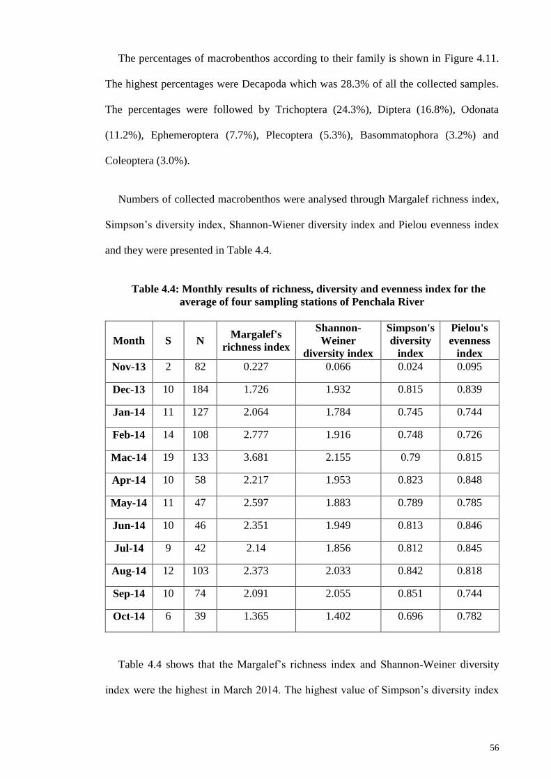
56
The percentages of macrobenthos according to their family is shown in Figure 4.11.
The highest percentages were Decapoda which was 28.3% of all the collected samples.
The percentages were followed by Trichoptera (24.3%), Diptera (16.8%), Odonata
(11.2%), Ephemeroptera (7.7%), Plecoptera (5.3%), Basommatophora (3.2%) and
Coleoptera (3.0%).
Numbers of collected macrobenthos were analysed through Margalef richness index,
Simpson’s diversity index, Shannon-Wiener diversity index and Pielou evenness index
and they were presented in Table 4.4.
Table 4.4: Monthly results of richness, diversity and evenness index for the
average of four sampling stations of Penchala River
Month S N Margalef's
richness index
Shannon-
Weiner
diversity index
Simpson's
diversity
index
Pielou's
evenness
index
Nov-13 2 82 0.227 0.066 0.024 0.095
Dec-13 10 184 1.726 1.932 0.815 0.839
Jan-14 11 127 2.064 1.784 0.745 0.744
Feb-14 14 108 2.777 1.916 0.748 0.726
Mac-14 19 133 3.681 2.155 0.79 0.815
Apr-14 10 58 2.217 1.953 0.823 0.848
May-14 11 47 2.597 1.883 0.789 0.785
Jun-14 10 46 2.351 1.949 0.813 0.846
Jul-14 9 42 2.14 1.856 0.812 0.845
Aug-14 12 103 2.373 2.033 0.842 0.818
Sep-14 10 74 2.091 2.055 0.851 0.744
Oct-14 6 39 1.365 1.402 0.696 0.782
Table 4.4 shows that the Margalef’s richness index and Shannon-Weiner diversity
index were the highest in March 2014. The highest value of Simpson’s diversity index

57
was in September 2014 and the highest Pielou’s evenness index was recorded in April
2014. All the indexes were at the lowest in November 2013.
4.3 Statistical analysis
Pearson correlation coefficient (r) among the WQI value with its parameter and
biological indices were performed to find degree of significance relationship among the
parameters. The results were summarised in Table 4.5.
From the table, the WQI value was significantly correlated with pH (r= 0.813; P=0.01).
The pH variable was found negatively significantly affected by BOD, r= -0.749; P=0.005.
WQI value was found negatively significantly correlated with Margalef’s richness index,
r= -0.735; P=0.007, Shannon-Weiner diversity index, r= -0.642; P=0.024, Simpson’s
diversity index, r= -0.618; P=0.032 and Pielou’s evenness index, r= -0.589; P=0.044. On
the other hand, the table also shown that there were high positive correlation between all
the biotic indices.

58
Table 4.5: Pearson’s correlation of coefficients (r) of physico-chemical parameters and biotic indices of Penchala River
Parameters
Correlation coefficient (r)
WQI Temp pH DO NH3-N BOD COD TSS Margalef Shannon
- Weiner
Simpson Pielou
WQI 1
Temp -0.077 1
pH 0.813** -0.259 1
DO 0.292 0.307 0.245 1
NH3-N -0.565 0.310 -0.482 0.399 1
BOD -0.649* 0.164 0.749** -0.110 0.230 1
COD -0.287 0.647* 0.019 -0.579 -0.306 -0.018 1
TSS -0.032 -0.360 0.174 -0.47 -0.148 -0.029 0.107 1
Margalef -0.735** 0.066 -0.611* -0.232 0.249 0.693* -0.016 0.176 1
Shannon-
Weiner
-0.642* -0.65 -0.467 -0.314 0.155 0.618* 0.101 0.444 0.844** 1
Simpson -0.618* -0.080 -0.469 -0.348 0.136 0.586* 0.156 0.439 0.736** 0.976** 1
Pielou -0.589* 0.016 -0.490 -0.340 0.112 0.575 0.130 0.319 0.706* 0.936** 0.977** 1
**. correlation is significant at the 0.01 level (2-tailed), P<0.01
*. correlation is significant at the 0.05 level (2-tailed), P<0.05

59
CHAPTER 5: DISCUSSION
5.1 Variation of physico-chemical parameters at Penchala River
Water Quality at Penchala River is unique as it has a wide range of WQI. Results that
come from water sampling in this study served as the current water quality status for
Penchala River. The results show that the WQI were in the range of 58.1 to 71.0. Results
on WQI presented in Chapter 4 shows that Station 1 has the best quality of water
compared to Station 2, 3 and 4. As mentioned before, Station 1 has the natural physical
characteristics with various types of gravel, rocky slopes and existence of aquatic plants.
All of these elements are very important for river restoration. The cleanliness of the river
gives opportunity to the local authority to build up a recreation park for the community
to enjoy the panoramic view. In order to maintain the river health, a list of rules and
regulations was set up and being closely monitored by the local authority.
The deterioration of WQI at Station 1 in September 2014 was caused by the temporary
construction activities at the river bank. The construction was held to widen the river
before the water entering the recreational park. As the construction begun, the flow has
been stuck (0.1815 m/s) and the water started to overflow. The results for TDS (33.62
mg/L) was the highest and the water became cloudy (181 NTU). The situation become
worst as the contractor did not cover the exposed river bank and soil erosion deposited at
the river bottom.

60
Figure 5.1: Overflow at Station 1 during construction in September 2014
WQI at Station 2 was sometimes up and down, which is mostly caused by the
anthropogenic activities. The WQI was improved at the end of the sampling routine and
perhaps the improvement will be prolonged as many construction and renovation have
been carried out.
Results for WQI at Station 3 were relatively stable with no drastic changes in value
through the sampling dates. The data shows only small difference even though there was
heavy rain a day before and construction in progress at Station 2. The results for WQI
were in the range of 46.2 to 65.2, and all of the values were classified into Class III and
Class IV. Results for Conductivity (471.0 µs/cm) and TDS (235.0 mg/L) were the highest
in June 2014 as there were heavy rain early in the morning. It was supported by physical
data on velocity. The velocity was the highest in June 2014 which was 0.4400 m/s.
Station 4 was located at the downstream. The WQI at this station was the worst among
all the stations with WQI in the range of 42.4 – 61.8. This situation happened probably
because of all the pollutant from the upper stream accumulated and flowing through this

61
station. Other than that, there are squatter’s area located near to the river bank. The river
water quality falls into Class III and Class IV which classified under ‘polluted’ water.
In generally, Station 4 had the worst WQI at the beginning but the WQI were improved
as the abandoned wooden cages in the middle of the river was removed. The removal
made the river flows smoothly. Another factor that negatively affected the WQI data for
this station was construction activities in December 2013 to build concrete river bank.
During the construction, the WQI status had dropped from ‘slightly polluted’ to
‘polluted’. The most affected parameter was turbidity. The turbidity was low which was
21.2 NTU in November 2013 but the results were suddenly rose up to 95.9 mg/L in
December 2013 and reached to 123.0 mg/L in February 2014. The results were supported
by results on the concentration of suspended solids. The concentration of suspended
solids was 51 mg/L in December 2013 and 24 mg/L in February 2014.
The results of temperature were the highest at Station 4 which was in the range of
27.4℃ – 31.4 ℃ and lowest at Station 1 which was in the range of 24.7℃ – 26.5℃. The
high temperature at Station 4 was due to direct sunlight penetrates into water. From the
observation, there was no riparian vegetation cover at the river bank. This situation
results in a low concentration of dissolved oxygen (0.16 – 2.41 mg/L) as the water had
less ability to hold oxygen molecule.
Dissolved oxygen in the water gains from the atmosphere and also from
photosynthesis by aquatic plants. In addition, the running water contains a higher
concentration of DO compared to still water because it churning that can dissolve more
oxygen whereas activities such as respiration by aquatic animals, decomposition of
organic matter and various chemical reactions will lower the concentration of DO. Other
than that, if more oxygen is consumed than is produced, DO levels will decline and some
sensitive macrobenthos may move away, weaken or die (Rapport and Whitford, 1999).

62
The fluctuation in concentration of DO is also affected by water temperature and
altitude. Cold water holds more oxygen than warm water and lower altitude will hold
more oxygen compared to higher altitudes (Schmidt-Nielson, 2010). The low
concentration of DO also caused by decreased amount of oxygen consumption for
decomposition of biological and chemical substances. This statement was supported by
the high concentration of COD and BOD at Station 2, 3 and 4.
The results of BOD and COD at Station 2 was the highest in August 2014 which was
11.64 mg/L and 81.0 mg/L, respectively. The high results were supported by the result
of the concentration of DO. The results for DO were low (1.55 mg/L) in August 2014,
which indicates that the concentration of oxygen that dissolved in the water was so much
consumed by the bacteria to decompose organic material in the water and the high results
of COD in August 2014 indicate that the decomposition of organic materials were high
at this station. Other than that this situation also had caused unpleased foul odor as the
anaerobic decomposition which produces methane gas.
The concentration of ammoniacal nitrogen and phosphate were the highest at Station
2 which was in the range of 0 – 6.42 mg/L and 0.4 – 1.60 mg/L, respectively. From the
observation, there were direct sullage discharges from both sides and garbages floating
and stuck on the river bank. Discharges from these two areas boost the concentration of
nutrients such as ammoniacal nitrogen and phosphate. This data was supported by
observation at the bottom of the river was green, which indicates algae was so well
growing.
Table 5.1 present comparison results between previous and current study conducted
at Penchala River. Study by Ismail et al., (2014) was conducted from 1997 to 2005 and
Mahazar et al., (2013) was conducted from April to August 2012. From the table, the
results show that there is improvement for all the parameters especially for WQI value.
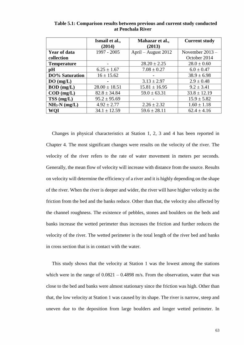
63
Table 5.1: Comparison results between previous and current study conducted
at Penchala River
Ismail et al.,
(2014)
Mahazar et al.,
(2013)
Current study
Year of data
collection
1997 - 2005 April – August 2012 November 2013 –
October 2014
Temperature - 28.20 ± 2.25 28.0 ± 0.60
pH 6.25 ± 1.67 7.08 ± 0.27 6.0 ± 0.47
DO% Saturation 16 ± 15.62 - 38.9 ± 6.98
DO (mg/L) - 3.13 ± 2.97 2.9 ± 0.48
BOD (mg/L) 28.00 ± 18.51 15.81 ± 16.95 9.2 ± 3.41
COD (mg/L) 82.8 ± 34.84 59.0 ± 63.31 33.8 ± 12.19
TSS (mg/L) 95.2 ± 95.69 - 15.9 ± 5.82
NH3-N (mg/L) 4.92 ± 2.77 2.26 ± 2.32 1.60 ± 1.18
WQI 34.1 ± 12.59 59.6 ± 28.11 62.4 ± 4.16
Changes in physical characteristics at Station 1, 2, 3 and 4 has been reported in
Chapter 4. The most significant changes were results on the velocity of the river. The
velocity of the river refers to the rate of water movement in meters per seconds.
Generally, the mean flow of velocity will increase with distance from the source. Results
on velocity will determine the efficiency of a river and it is highly depending on the shape
of the river. When the river is deeper and wider, the river will have higher velocity as the
friction from the bed and the banks reduce. Other than that, the velocity also affected by
the channel roughness. The existence of pebbles, stones and boulders on the beds and
banks increase the wetted perimeter thus increases the friction and further reduces the
velocity of the river. The wetted perimeter is the total length of the river bed and banks
in cross section that is in contact with the water.
This study shows that the velocity at Station 1 was the lowest among the stations
which were in the range of 0.0821 – 0.4898 m/s. From the observation, water that was
close to the bed and banks were almost stationary since the friction was high. Other than
that, the low velocity at Station 1 was caused by its shape. The river is narrow, steep and
uneven due to the deposition from large boulders and longer wetted perimeter. In

64
addition, the velocity of flowing water is slower since there is more energy needed to
overcome friction between the uneven river bed. Eventhough the flow at Station 1 appear
to be faster it is actually all the energy is lost since a lot of energy is expended to
overcome friction and uneven river bed.
Results on velocity at Station 4 show that the results for velocity were relatively low
compared to other stations. From the observation, the velocity was low because of an
abandoned wooden cage at the center of the river. The cages caused all the solid waste
such as garbage and plastic bags were stuck at it thus slow down the water flow. On July
2014, the abandoned wooden cages have been removed thus improve the velocity from
0.0871 m/s (June 2014) to 0.3610 m/s (July 2014) and reached 0.593 m/s in August 2014.
The result of water discharge at Station 2 was the highest and become worse perhaps
affected by construction activities in January 2014. The extreme results were caused by
the construction activities as there was a bulk of white stone and sand at the river's edge.
Results show that the water level had risen to 0.45 m. The stone has caused the width
decreased circumstantially increased the velocity up to 0.5710 m/s.
Figure 5.2: White boulders at Station 2 during construction in January 2014

65
5.2 Variations of macrobenthos at Penchala River
Based on the results presented in Chapter 4, the results on biodiversity index, which
consist of diversity index, species richness and evenness of macrobenthos at Penchala
River determined that river has relatively high index for richness, diversity and evenness
index.
Margalef richness index (2.13) value at Penchala River indicate that the river is clean
as the index is upper than 1.0. The value at Station 2 and 3 were give us information that
the river was slightly polluted (Lenat et al., 1988). Shannon-Weiner diversity index
values were also high at this river with 1.75. Shannon-Weiner diversity index values
above 3.0 indicate that the habitat structure is stable while values less than 1.0 indicate
that the river has been polluted (Mandaville, 2002). The Simpsons index value varies
from 1.0 to 0. The 1.0 indicate that the habitat is stable while 0 indicate that the habitat
was degraded. The Penchala River recorded 0.73 for Simpson’s index indicate that the
diversity is relatively high. Values on Pielou’s evenness index were 0.74. The value is
closer to 1.0 indicates that the macrobenthos were evenly distributed at Penchala River
(Pielou, 1966).
This study also shows that sampling method using Surber’s net was suitable as many
orders with different families has been collected during the sampling. As the results, there
were 8 orders with 23 families were collected at Station 1, 2 orders with 3 families at
Station 2, 4 orders with 8 families at Station 3 and 1 order with 2 families at Station 4.
From the results, the data show that the Clean (Station 1) has the highest numbers of
orders and family while Polluted (Station 4) has the lowest numbers of orders and
families. The findings had proved that the clean river which the WQI falls under Class I
and II was suitable for survival of macrobenthos such as Ephemeroptera, Plecoptera,

66
Trichoptera, Odonata, Coleoptera, and Decapoda. These orders of macrobenthos were
very sensitive to deterioration of water quality thus the existing of these orders indicated
the water quality was good and healthy. Contrast to existing of Diptera, Oligochaeta and
Basommatophora, these orders indicated that the water quality was slightly polluted and
not healthy.
5.3 Relationship of physico-chemical parameters and species diversity of
macrobenthos at Penchala River
The existence and diversity of macrobenthos at Station 1, 2, 3 and 4 during the
sampling period appeared to respond to the physico-chemical deterioration as reported
in Chapter 4. High numbers of macrobenthos at Station 1 was associated with the clean,
compatible and unpolluted condition.
Poor water quality or polluted water body is one of the limiting factors of the existence
and diversity of macrobenthos as they are highly responded to deterioration of water
quality status (Paul and Meyer, 2001). Different species of macrobenthos were responded
differently from one and another. The finding shows that the existence and distribution
of macrobenthos were influenced by physico-chemical and biological characteristic as
well as physical parameters of the river. The diversity was the highest at Station 1.
Numbers of Ephemeroptera, Plecoptera, and Tricoptera (EPT), Odonata and Decapoda
were abundant at Station 1 which was classified as clean and unpolluted area while
Chironomidae and Physidae were abundant at polluted sites.
This finding was parallel to study done by Mahazar et al. (2013) who found out that
the clean and unpolluted area have a high number of EPT, Crustacea and Isopoda while
the Blood-red Chironomidae, as well as other Dipterans, dominated in polluted areas.

67
The study also agreed on the decreasing of the diversity of macrobenthos from clean to
the polluted area. He also found that the Chironomidae was present consistently
throughout the polluted rivers.
The numbers of macrobenthos that exist at certain values of water quality status is
affected by the velocity. From the figures, it shows that a trend which the number of
macrobenthos has affected by the value of WQI at every station. Another finding that
could be extracted from then figure is the number of macrobenthos that is high response
to velocity. From the figures, the number of macrobenthos was increasing when the
velocity of the river was decreased.
The most abundance was Trichoptera on every sampling date. Trichoptera have a very
low value of pollution tolerance and it was very sensitive to water pollution. The number
of Trichoptera was decreased from March to July 2014 perhaps because of the
deterioration of water quality at Station 1. The second-high abundances were Odonata
and Ephemeroptera. Odonata and Ephemeroptera have also low values of pollution
tolerance. All these three orders only exist in clean and unpolluted river water. The
number decreased as the water quality index was decreased.
Ephemeroptera is very sensitive to the deterioration of water quality and their
existence at Station 1 signified relatively clean conditions (Merritt and Cumins, 1978).
To support the statement, the data collected shows that Ephemeroptera only exists at
Station 1 and absent at Station 2, 3 and 4. The Trichopteran caddisflies were found as
good biological indicators of the clean river since they also only exist at Station 1.
Station 2 and 3 were dominantly by Diptera Chironomidae. The low concentration of
dissolved oxygen creates a suitable environment for Diptera Chironomidae to survive
and reproduce. Diptera Chironomidae is a unique macrobenthos as it possesses

68
haemoglobin in their blood which makes them survive in waters that have a very little
oxygen (Carew et al., 2007). This theory was supported by an abundance of
Chironomidae were collected during the sampling at this station, supported by the low
concentration of DO which was in the range of 0.65 – 2.7 mg/L in November 2014
compared to other stations. Other than that, patterns of the existence of the Chironomidae
were influenced by the available quantity and quality of larval food. In addition, the
species composition may change influenced by the changes of particle composition
especially the deposition of organic matter and detritus on the bottom (Galdean et al,
2000).
Nutrient in river water refers to the concentration of nitrogen and phosphate or known
as eutrophication. The eutrophication and organic matter affected the existence and
diversity of macrobenthos as the production of algae and other vegetation are increasing
which provide substrate, shelter and food for macrobenthos. Generally, increasing of
organic matter in the river will reduce the number of macrobenthos as an example of
Trichoptera as high loads of organic materials promote a complete deoxygenation
condition. Even though the oxygen is very limited; the Oligochaetes, Chironomidae and
Simuliidae are the macroinvertebrates which still can survive in high numbers.
Numbers of Basommatophora Physidae also can be found near to the river's edge at
Station 2 which the velocity was very low and nearly stagnant. The water flow had been
blocked by either rock, deposition of sands or solid wastes. Even though the
concentration of dissolved oxygen was low and the velocity was also low, Physidae can
survive it has a lung structure for their breathing mechanism (Koopman et al., 2016).
Macrobenthos was the most abundance and high diversity at Station 1. Station 1 have
a good canopy cover that maintain the temperature. The changes of temperature may
result from industrial discharges, agricultural and forestry activities and removal of

69
riparian vegetation as well as channelisation and regulation of streams. Slight changes of
temperature can affect the ecology of aquatic insects as it may change the flow condition,
the rate of production and mineralisation. The macrobenthos are sensitive to temperature
and they will move to the optimal temperature for their survival. In addition, temperature
also affects the oxygen content in the water as the oxygen levels become lower as the
temperature increases. The increasing of temperature can cause by weather, removal of
shading streambank vegetation, impoundments which a body of water confined by a
barrier such as a dam), discharge of cooling water, urban storm water and groundwater
inflows to the stream (Brungs and Jones 1977). For example, the optimum temperature
of 20oC is the lethal level for Plecoptera and Ephemeroptera. The Chironomidae and
Odonata can be generally found at a slightly high temperature which is around 40oC.
Other than that, the high canopy cover provides additional foods to the macrobenthos.
The leaf litter in the river also create an extra habitat for macrobenthos. The Coleoptera
can be found mostly in between the dried leaves.
Presence of sensitive families like Ephemeroptera, Plecoptera and Tricoptera at
Station 1 and they were absent at Station 2, 3 and 4. These groups have a very low
pollutant tolerance thus the presence of these group indicated clean river and the
discontinuity in the presence of these group denotes that the water quality status has been
degraded.
The diversity of macrobenthos was also low at Station 3. It is a low diversity because
there was only free flow river water. Most of the macrobenthos attached at the gravels,
rocks and even at the solid waste but all of these potential habitats were absent at this
station. The dipterans were survived by attaching to secondary grass that grows at the
river's edge.

70
There was no other macrobenthos were found at station 4 except Basommatophora
Physidae and Thiaridae. The Physidae and Thiaridae can be found at the side of the river
bank. The very low water velocity was not an ideal place for breeding, and low
concentration of dissolved oxygen was very as well as polluted water quality status.
Physidae and Thiaridae have a very high value of pollution tolerance (Nelson, 2011).
Thus, even though water quality at Station 4 were poor, both still can survive.
Other than that, the study also found out that the existence and distribution of
macrobenthos were also influenced by the physical characteristics of the river. The role
of the substrate of the river bed and the presence of aquatic plant are very important as
they serve as favoured habitat. Aquatic plant comprised of emergent, floating and
submerged plants. It provides shelter, egg laying sites, nursery areas and food sources for
herbivores.
For this study, the concrete river consists of sand and absence of aquatic plants make
it not suitable for breeding and serving as habitat for macrobenthos. Mandaville (2000)
agreed that macrobenthos has their specific preference upon the surrounding
environment as well the substrate to live on. This statement is parallel to the finding
obtained from this study. The same condition occurs at Station 2, 3 and 4 which the
concrete shaping the river. The modification of their habitat becomes the limiting factor
as it limits the ranges of a suitable niche for diverse macrobenthos to fill in the ecosystem.
Other than that, the aquatic plants only occur at the river bank. In this case, water quality
and the velocity become the limiting factor. The results obtained show that the numbers
and diversity of macrobenthos decrease from upstream (Station 1) toward the
downstream (Station 2, 3 and 4).
Significant physical factors that influence the existence and distribution of
macrobenthos are streamflow, current velocity, channel shape, water depth, substrate and

71
temperature. Increasing of water level will result in inundation of physical structures and
features. When these events happened, it demolished the substrates that are important for
colonisation and attachment of invertebrates and also act as habitat for feeding, shelter,
current refuge and spawning and represent an increase in the quantity, diversity and
complexity of physical habitat for both invertebrates and fish (Crowder and Cooper,
1982; Crook and Robertson 1999)
Low velocity and shallow areas serve as a very suitable condition for the growth of
aquatic macrophytes. Macrophytes are widely recognised as important habitat for some
invertebrates and fish as it is a source of food and serve as protection area from predators
and current as well as increase the amount of available habitat per unit area of substrate
(Crowder and Cooper, 1982; Minshall, 1988; Newman et al. 1992; Weatherhead and
James, 1991).
In a different perspective, high velocity is important too. High velocity helps to flush
of fine sediments and organic matter from areas of coarse streambed substrate. This
flushing reduces armouring of the stream bed and leads to greater availability of
interstitial spaces in the coarser substrate. These spaces are available as habitat for
invertebrates.
The increasing number of solids in a river is as the result of erosion, farming, forestry
or mining activities which located near to the river bank. The solids have been identified
to give effect neither direct nor indirect as it affects water clarity. High concentration of
solids in water body decreases the passage of light through water thus slowing
photosynthesis by aquatic plants. Other than that, solids also will make the water heating
up rapidly as the solids particle will hold more heat thus indirectly affected macrobenthos
which intolerant with the deterioration of water temperature (APHA, 1992).

72
The effect from the concentration of heavy metals becomes one of the concerns as the
urban river flows through the industrial area. Heavy metals are well known as a source
of the toxicity problem to both aquatic organism and human (Beasley and Kneale, 2003).
Generally, aquatic insects are more tolerant to heavy metals compared to fish and other
invertebrates. A study by Qu et al., (2010) had found out that the total abundance and
species richness of macrobenthos were decreased when the concentration of heavy metals
increased. They also mentioned that although the effects were compounded by different
factors such as altitude, temperature, stream width and turbidity, the influence of heavy
metals on macrobenthos communities was clearly identified eventhough the
concentration is not seriously high. Parallel to their study, Hickey and Clements (1998)
were agreed that there were significance effects from the high concentration of heavy
metals to the existence and diversity of macrobenthos. They also suggested that
abundance of mayflies, species richness of mayflies, the number of EPT taxa and total
taxonomic richness are the most useful indicators of heavy metal pollution in New
Zealand streams.
Optimum habitat condition also plays as the important role that influences the
existence and diversity of macrobenthos. The habitats are defined as a complex
interaction between physical factors and the ecological requirements of aquatic flora and
fauna such as light, shelter, food and flow-mediated chemical exchanges. Macrobenthos
can survive all parts of the water body. Some of them live on the water’s surface, in the
water, in the sediment, on the bottom and also on submerged rocks, logs and leaf litter.
Dudgeon (2008) had summarized that the aquatic habitat is adversely impacted by
urbanization, deforestation, construction, irrigation, drainage, wetlands and pollution.
Other than that, it also depends on the interactions of hydrology, geomorphology features
and structural elements. Examples of geomorphological features are pools, bars, benches,

73
overhanging banks and anabranches, and examples of structural elements are boulders,
tree roots, coarse woody debris and macrophytes.
Other important physical habitat features for macrobenthos are cover and refuge as
well as conditions of its river bank and shore. These features are usually provided by
boulders, large wooden debris, aquatic vegetation, water turbulence and depth. It
provides shelter from predators and alteration of physical condition such as fast current
and sunlight. The ‘slack water’ area also plays as important role as habitat for
macrobenthos (Marchese et al., 2002). The slack water is a typical small shallow area of
still water that formed by sand bars, woody debris and bank morphology. It is important
to provide refuge from current for the young stages of fish and shrimp and predation and
as sites where food is abundant as it has a greater amount of benthic organic matter which
a potential food resource for shrimp (Humphrises et al., 2006; Richardson et al., 2004;
Burns and Walker, 2000).

74
CHAPTER 6: CONCLUSION
Rapid urbanisation in Malaysia causes alterations of the physico-chemicals and
hydraulics characteristics that affect the existence and diversity of macrobenthos
communities. This study agreed that deterioration of water quality characteristics is
affected by urbanisation. Eventhough urbanisation does not affect directly to the
existence and diversity of macrobenthos, it does alter the physico-chemical and
hydraulics characteristics of a natural river which in turn affect the macrobenthos
communities. This study also understood that any modification of the physical and
chemical characteristics of a habitat had changed the existence and diversity of
macrobenthos.
The current water quality status at Penchala River is in the range of WQI 58.1 to 71.0.
This study found that the factors that affect the water quality are alteration of river
structure and human activities in and around the river. The significant pollutant that affect
the water quality for Station 1 was total dissolved solids. For Station 2 and 3, the high
concentration of ammoniacal nitrogen, phosphate and organic pollutants as well as
deterioration of velocity gave impact to existence and diversity of macrobenthos. Station
4 was highly affected by human such as squatters and construction activities at the river
bank.
This study also shows that the macrobenthos has been successfully act as biological
monitoring agent. It is useful in detecting transient and long term pollution of urban
rivers. The aim of this study is achieved as macrobenthos had been proved as it serves as
an alternative way in determination of water quality status at urban river, the existence
and diversity of macrobenthos were highly responded to the alteration of water quality at
identified stations.
75
Macrobenthos are very useful to determine river health status by virtue of their role in
the aquatic ecosystem. It utilised minimal cost, cheap and give rapid results on
deterioration of water quality at Penchala River. It gives early warnings of hazards,
detecting pollutant and further provides information for monitoring and evaluating the
environmental effects.
The macrobenthos were collected by using Surber net. The results show that there
were 1043 macrobenthos were collected during the sampling period. Form the number,
there were 465 (44%), 176 (17%), 372 (36%) and 30 (3%) macrobenthos were existed at
Station 1, 2, 3 and 4 respectively. The sensitive group of Ephemeroptera, Plecoptera and
Tricoptera (EPT) group at Station 1 indicated that the river is clean. Diptera
Chironomidae and Basommatophora Physidae were abundance at Station 2, 3 and 4 as
they can survive in slightly polluted river as they have higher level of tolerance towards
pollution. In addition, Physidae has special gill structure for respiration.
The advantages of using macrobenthos as biological indicator as their abundance
existence and ubiquitous in nature. In addition, the macrobenthos also have sedentary
lifestyle and long lifespan thus make them suitable as pollutant indicator. Other than that,
the macrobenthos also relatively rich with families that responses to environmental
changes both natural and man-induced during their life cycle.
The positive results on correlation analysis support the finding. The analysis shows
that there is strong correlation between water quality index with Margalef richness index
(2.13), Simpsons diversity index (0.73), Shannon-Weiner diversity index (1.75) and
Pielou evenness index (0.74) indicated that biological monitoring at Penchala River by
using macrobenthos can be served as an alternative way to determine the river health.

76
For further development, a comprehensive approach is needed specially to determine
the effects of human activities on aquatic ecosystems. Understanding of the contribution
on the aquatic ecosystem is important such as the river continuum hypothesis, path
dynamics as well as the importance of variation in the physical environment especially
annual shifts in distribution and amount of rainfall and runoff. Other than that, a series
of quality control provision is also highly recommended.
Other than that, the ecological principals have to be up-to-date to the current
conceptual foundation as developed countries will come out with new approaches with
latest research papers from time to time. The current study is suggested to be done at
other urban rivers under controlled condition. This is important in order to avoid any
unexpected activities from the local authorities. If this situation occurs in the future, it is
suggested that the study period can be extended until the situation back to normal
condition. This is to see the impact of these activities to the study area and to further
understand about river restoration.
It is further suggestion to achieve the maximum numbers of healthy urban river, all
the programmes need involvement of all stakeholders including the local communities,
NGOs, water management professionals and scientists as well as decisions makers and
policy makers at all level of government.

77
REFERENCES
Ab Hamid, S., & Rawi, C. S. M. (2014). Ecology of Ephemeroptera, Plecoptera and
Trichoptera (Insecta) in rivers of the Gunung Jerai Forest Reserve: Diversity and
distribution of functional feeding groups. Tropical Life Sciences Research, 25(1),
61.
Al-Shami, S. A., Rawi, C. S. M., Ahmad, A. H., Hamid, S. A., & Nor, S. A. M. (2011).
Influence of agricultural, industrial, and anthropogenic stresses on the distribution
and diversity of macroinvertebrates in Juru River Basin, Penang,
Malaysia. Ecotoxicology and Environmental Safety, 74(5), 1195-1202.
Al-Shami, S. A., Salmah, M. R. C., Hassan, A. A., & Azizah, M. N. S. (2010). Temporal
distribution of larval Chironomidae (Diptera) in experimental rice fields in
Penang, Malaysia. Journal of Asia-Pacific Entomology, 13(1), 17-22.
Cairns, J., & Dickson, K. L. (Eds.). (1973). Biological methods for the assessment of
water quality. ASTM.
Anbuchezhian, R. M., Rameshkumar, G., & Ravichandran, S. (2009). Macrobenthic
composition and diversity in the coastal belt of Thondi, southeast coast of
India. Global Journal of Environmental Research, 3(2), 68-75.
Anzecc, A. (2000). Australian and New Zealand guidelines for fresh and marine water
quality. Australian and New Zealand Environment and Conservation Council
and Agriculture and Resource Management Council of Australia and New
Zealand, Canberra, 1-103.
Federation, W. E., & APH Association. (2005). Standard methods for the examination of
water and wastewater. American Public Health Association (APHA):
Washington, DC, USA.
Arslan, N., Salur, A., Kalyoncu, H., Mercan, D., Barişik, B., & Odabaşi, D. A. (2016).
The use of BMWP and ASPT indices for evaluation of water quality according
to macroinvertebrates in Küçük Menderes River (Turkey). Biologia, 71(1), 49-
57.
Aschengrau, A. & Seage, G. R. (2007). Essentials of epidemiology in public health,
second edition. Sudbury, MA: Jones and Bartlett Publishers, 137.

78
Aweng, E. R., Suhaimi, O., & Nur Izzati, S. (2012). Benthic macroinvertebrate
community structure and distribution in Sungai Pichong, Gunung Chamah,
Kelantan, Malaysia. American International Journal of Contemporary
Research, 2(1), 163-167.
Azrina, M. Z., Yap, C. K., Ismail, A. R., Ismail, A., & Tan, S. G. (2006). Anthropogenic
impacts on the distribution and biodiversity of benthic macroinvertebrates and
water quality of the Langat River, Peninsular Malaysia. Ecotoxicology and
environmental safety, 64(3), 337-347.
B. W. Pennak, Freshwater Invertebrate of the United States, New York: Litton
Educational Publishing Inc., 1978, 45-68.
Balogh, K. V. (1988). Comparison of mussels and crustacean plankton to monitor heavy
metal pollution. Water, Air, and Soil Pollution, 37(3-4), 281-292.
Barton, D. R., & Metcalfe-Smith, J. L. (1992). A comparison of sampling techniques and
summary indices for assessment of water quality in the Yamaska River, Québec,
based on benthic macroinvertebrates. Environmental Monitoring and
Assessment, 21(3), 225-244.
Baudo, R., & Galanti, G. (1988). Unio elongatulus as indicator of trace element
pollution. Internationale Vereinigung fuer Theoretische und Angewandte
Limnologie. Verhandlungen IVTLAP, 23(3).
Beach, D. (2003). Coastal sprawl: The effects of urban design on aquatic ecosystems.
In of the United States, Pew Oceans Commission 2002.
Beasley, G., & Kneale, P. E. (2003). Investigating the influence of heavy metals on
macro-invertebrate assemblages using Partial Cononical Correspondence
Analysis (pCCA). Hydrology and Earth System Sciences Discussions, 7(2), 221-
233.
Berndtsson, J. C. (2010). Green roof performance towards management of runoff water
quantity and quality: a review. Ecological Engineering, 36(4), 351-360.
Bernhardt, E. S., & Palmer, M. A. (2007). Restoring streams in an urbanizing
world. Freshwater Biology, 52(4), 738-751.
Birol, E., Karousakis, K., & Koundouri, P. (2006). Using economic valuation techniques
to inform water resources management: A survey and critical appraisal of
available techniques and an application. Science of the Total
Environment, 365(1), 105-122.

79
Blanco, S., & Bécares, E. (2010). Are biotic indices sensitive to river toxicants? A
comparison of metrics based on diatoms and macro-
invertebrates. Chemosphere, 79(1), 18-25.
Blijswijk, W. V., Coimbra, C. N., & Graça, M. A. (2004). The use of biological methods
based on macroinvertebrates to an Iberian stream (Central Portugal) receiving a
paper mill effluent. Limnetica, 23(3-4), 307-314.
Bonada, N., Prat, N., Resh, V. H., & Statzner, B. (2006). Developments in aquatic insect
biomonitoring: a comparative analysis of recent approaches. Annual Review
Entomology, 51, 495-523.
Bonell, M. (2002). Ecohydrology—A completely new idea?. Hydrological Sciences
Journal, 47(5), 809-810.
Bouchard, J. (2012). Guide to aquatic invertebrate families of Mongolia. Identification
Manual for Students, Citizen Monitors, and Aquatic Resource Professionals.
Saint Paul, Minnesota, USA.
Bratrich, C., Truffer, B., Jorde, K., Markard, J., Meier, W., Peter, A., ... & Wehrli, B.
(2004). Green hydropower: a new assessment procedure for river
management. River Research and Applications, 20(7), 865-882.
Brookes, A., & Shields, F. D. (Eds.). (1996). River channel restoration: guiding principles
for sustainable projects. Chichester: Wiley.
Brooks, A. P. Brooks AP, Abbe TB, Jansen JD, Taylor M, Gippel CJ (2001). Putting the
wood back into our rivers: an experiment in river rehabilitation. In: Rutherfurd
ID, Sheldon F, Brierley GJ, Kenyon C (eds), 3rd Australian Stream Management
Conference Proceedings—The Value of Healthy Streams, 73–80.
Brungs, W.S. and B.R. Jones. 1977. Temperature Criteria for Freshwater Fish: Protocols
and Procedures. EPA-600/3-77-061. Environ. Research Lab, Ecological
Resources Service, U.S. Environmental Protection Agency, Office of Research
and Development, Duluth, MN.
Bunn, S. E., & Arthington, A. H. (2002). Basic principles and ecological consequences
of altered flow regimes for aquatic biodiversity. Environmental
Management, 30(4), 492-507.

80
Burns, A., & Walker, K. F. (2000). Biofilms as food for decapods (Atyidae,
Palaemonidae) in the River Murray, South Australia. Hydrobiologia, 437(1), 83-
90.
Cao, Y., Bark, A. W., & Williams, W. P. (1997). Analysing benthic macroinvertebrate
community changes along a pollution gradient: a framework for the development
of biotic indices. Water Research, 31(4), 884-892.
Carew, M. E., Pettigrove, V., Cox, R. L., & Hoffmann, A. A. (2007). The response of
Chironomidae to sediment pollution and other environmental characteristics in
urban wetlands. Freshwater Biology, 52(12), 2444-2462.
Carter, J. L., & Resh, V. H. (2013). Analytical approaches used in stream benthic
macroinvertebrate biomonitoring programs of State agencies in the United
States. US Geological Survey Open File Report, 1129.
Chan, N. W. (1997, August). Mitigating natural hazards and disasters in Malaysia:
Lessons learnt from tropical storm greg and its aftermath. In K. S. Jomo
(Ed.), Proceedings of the First International Malaysian Studies Conference ,11-
13.
Chan, N. W. (2002). Rivers: towards sustainable development Penang: Penerbit
Universiti Sains Malaysia.
Chan, N. W. (2012). Managing urban rivers and water quality in Malaysia for sustainable
water resources. International Journal of Water Resources Development, 28(2),
343-354.
Ching, Y. C., Lee, Y. H., Toriman, M. E., Abdullah, M., & Yatim, B. B. (2015). Effect
of the big flood events on the water quality of the Muar River,
Malaysia. Sustainable Water Resources Management, 1(2), 97-110.
Chop, A. K., Jusoh, J., & Chan, N. W. (2002). The Klang river cleanup
programme. Rivers: Towards Sustainable Development, 378-389.
Compin, A., & Céréghino, R. (2007). Spatial patterns of macroinvertebrate functional
feeding groups in streams in relation to physical variables and land-cover in
Southwestern France. Landscape Ecology, 22(8), 1215-1225.
Cook, S. E. (1976). Quest for an index of community structure sensitive to water
pollution. Environmental Pollution (1970), 11(4), 269-288.

81
Couceiro, S. R. M., Hamada, N., Forsberg, B. R., Pimentel, T. P., & Luz, S. L. B. (2012).
A macroinvertebrate multimetric index to evaluate the biological condition of
streams in the Central Amazon region of Brazil. Ecological Indicators, 18, 118-
125.
Courtney, L. A., & Clements, W. H. (1998). Effects of acidic pH on benthic
macroinvertebrate communities in stream microcosms. Hydrobiologia, 379(1),
135-145.
Crook, D. A., & Robertson, A. I. (1999). Relationships between riverine fish and woody
debris: implications for lowland rivers. Marine and Freshwater Research, 50(8),
941-953.
Crowder, L. B., & Cooper, W. E. (1982). Habitat structural complexity and the
interaction between bluegills and their prey. Ecology, 63(6), 1802-1813.
Cummins, K. W., Merritt, R. W., & Andrade, P. C. (2005). The use of invertebrate
functional groups to characterize ecosystem attributes in selected streams and
rivers in south Brazil. Studies on Neotropical Fauna and Environment, 40(1), 69-
89.
Darracott, A., & Watling, H. (1975). The use of molluscs to monitor cadmium levels in
estuaries and coastal marine environments. Transactions of the Royal Society of
South Africa, 41(4), 325-338.
David D. Breshears (2005) An Ecologist's Perspective of Ecohydrology. Bulletin of the
Ecological Society of America 86:296–300.
Davis, A. P., & McCuen, R. H. (2005). Stormwater management for smart growth. 1st
edition. Springer Science & Business Media., New York.
De Jonge, M., Van de Vijver, B., Blust, R., & Bervoets, L. (2008). Responses of aquatic
organisms to metal pollution in a lowland river in Flanders: A comparison of
diatoms and macroinvertebrates. Science of The Total Environment, 407(1), 615-
629.
De Pauw, N., & Hawkes, H. (1994). Biological monitoring of river water quality. River
water quality monitoring and control. W.J. Walley & S. Judd (Eds). Aston
University, Birmingham.
De Pauw, N., & Vanhooren, G. (1983). Method for biological quality assessment of
watercourses in Belgium. Hydrobiologia, 100(1), 153-168.

82
Department of Environment Malaysia (DOE) (2011) Malaysia Environmental Quality
Report 2010. Department of Environmental, Ministry of Science, Technology
and the Environment Malaysia.
Department of Environment, Malaysia, (2002) Malaysia environmental quality report
2004. Department of Environment, Ministry of Sciences, Technology and the
Environment, Malaysia, Kuala Lumpur, Malaysia.
Department of Environment, Ministry of Natural Resources and Environment Malaysia
(2017, February 10). River water pollution sources. Retrieved February 15, 2017,
from https://www.doe.gov.my/portalv1/en/info-umum/punca-punca-kepada-
pencemaran-air-sungai/278
DOE Malaysia (2013) Environmental Report: River water quality monitoring program,
Department of Environment, Ministry of Natural Resources and Environment,
Government of Malaysia.
DOE Malaysia (2015) Environmental Report: River water quality monitoring program,
Department of Environment, Ministry of natural Resources and Environment,
Government of Malaysia.
DOE Malaysia (1994) Classification of Malaysian rivers. Final report on development of
water quality criteria and standards for Malaysia (Phase IV—River
Classification). Department of Environment (DOE) Malaysia, Ministry of
Natural Resources and Environment
Dudgeon, D., (2008) Tropical Streams Ecology. Elsevier, USA, 343
Dunbar, M. J., & Acreman, M. C. (2001). Applied hydro-ecological science for the
twenty-first century. Hydro-ecology: Linking hydrology and aquatic ecology. Int.
Assoc. of Hydrol. Sci. Publ, 266, 1-17.
Engel, S. R., & Voshell, J. R. (2002). Volunteer biological monitoring: can it accurately
assess the ecological condition of streams?. American Entomologist, 48(3), 164-
177.
EQA (1974), Environmental Quality Act Government of Malaysia, Environmental
Quality (Sewage and Industrial Effluent), Government of Malaysia.
Fathoni Usman, R. C. O., & Sidek, L. M. (2014). Mobile application for field knowledge
data of urban river catchment decision support system. In Proceedings of the
International MultiConference of Engineers and Computer Scientists (Vol. 1).

83
Finkenbine, J. K., Atwater, J. W., & Mavinic, D. S. (2000). Stream health after
urbanization. JAWRA Journal of the American Water Resources
Association, 36(5), 1149-1160.
Fontoura, A. P., & Moura, A. G. (1984). Effects of some industrial effluents in the
biological quality of the water of the river Lima.
Fore, L. S., & Grafe, C. (2002). Using diatoms to assess the biological condition of large
rivers in Idaho (USA). Freshwater Biology, 47(10), 2015-2037.
Furse, M. T., Moss, D., Wright, J. F., & Armitage, P. D. (1984). The influence of seasonal
and taxonomic factors on the ordination and classification of running‐water sites
in Great Britain and on the prediction of their macro‐invertebrate
communities. Freshwater Biology, 14(3), 257-280.
Galdean, N., Callisto, M., & Barbosa, F. A. R. (2000). Lotic ecosystems of Serra do Cipó,
southeast Brazil: water quality and a tentative classification based on the benthic
macroinvertebrate community. Aquatic Ecosystem Health & Management, 3(4),
545-552.
Gallardo, B., Gascón, S., Quintana, X., & Comín, F. A. (2011). How to choose a
biodiversity indicator–Redundancy and complementarity of biodiversity metrics
in a freshwater ecosystem. Ecological indicators, 11(5), 1177-1184.
Gamito, S. (2010). Caution is needed when applying Margalef diversity
index. Ecological Indicators, 10(2), 550-551.
García, L., Pardo, I., & Delgado, C. (2014). Macroinvertebrate indicators of ecological
status in Mediterranean temporary stream types of the Balearic
Islands. Ecological Indicators, 45, 650-663.
Gauch, H. G. (1982). Multivariate analysis in community ecology (No. 1). Cambridge
University Press.
Türkmen, G. E. N. C. E. R., & Kazanci, N. İ. L. G. Ü. N. (2010). Applications of various
biodiversity indices to benthic macroinvertebrate assemblages in streams of a
national park in Turkey. Review of Hydrobiology, 3(2), 111-125.
Gibson, G. R., Barbour, M. T., Stribling, J. B., Gerritsen, J., & Karr, J. R.
(1996). Biological Criteria: Technical guidance for streams and small
rivers (No. PB--96-209770/XAB; EPA--822/B-96/001). Environmental
Protection Agency, Washington, DC (United States). Office of Water.

84
Gilvear, D. (1999). James R. Karr and Ellen W. Chu, Restoring Life in Running Waters:
Better Biological Monitoring. Water, Air, and Soil Pollution, 116(3-4), 666-667.
Gore, J. A. (Ed.) (1985). Restoration of rivers and streams, Butterworth, Stoneham, 280
Graca, M. A. S., & Coimbra, C. N. (1998). The elaboration of indices to assess biological
water quality. A case study. Water Research, 32(2), 380-392.
Hannah, D. M., Wood, P. J., & Sadler, J. P. (2004). Ecohydrology and hydroecology: A
‘new paradigm’? Hydrological Processes, 18(17), 3439-3445.
Harding, R. (Ed.). (1998). Environmental Decision-Making: The roles of scientists,
engineers, and the public. Federation Press, 6-11
Hauer, F. R., & Lamberti, G. A. (Eds.). (2011). Methods in stream ecology. Academic
Press. 51-79
Hawkes, H. A. (1998). Origin and development of the biological monitoring working
party score system. Water Research, 32(3), 964-968.
Hellawell, J. M. (1986). Biological Indicators of Freshwater Pollution and Environmental
ManagementElsevier Applied Science. London, UK.
Hellawell, J. M. (Ed.). (2012). Biological indicators of freshwater pollution and
environmental management. Springer Science & Business Media.
Hering, D., Borja, A., Carstensen, J., Carvalho, L., Elliott, M., Feld, C. K., ... & Solheim,
A. L. (2010). The European Water Framework Directive at the age of 10: a critical
review of the achievements with recommendations for the future. Science of the
total Environment, 408(19), 4007-4019.
Hickey, C. W., & Clements, W. H. (1998). Effects of heavy metals on benthic
macroinvertebrate communities in New Zealand streams. Environmental
toxicology and chemistry, 17(11), 2338-2346.
Hill, B. H., Stevenson, R. J., Pan, Y., Herlihy, A. T., Kaufmann, P. R., & Johnson, C. B.
(2001). Comparison of correlations between environmental characteristics and
stream diatom assemblages characterized at genus and species levels. Journal of
the North American Benthological Society, 20(2), 299-310.

85
Hiwasaki, L., & Arico, S. (2007). Integrating the social sciences into ecohydrology:
facilitating an interdisciplinary approach to solve issues surrounding water,
environment and people. Ecohydrology & Hydrobiology, 7(1), 3-9.
Hocutt, C.H. (1981). Fish as Indicators of Biological Integrity. Fisheries 6(6), 28-30.
Howard P. (2014) What is hydrology and what do hydrologists do? The USGS Water
Science School. Retrieved February 11, 2017, from
https://water.usgs.gov/edu/hydrology.html
Humphries, P., Cook, R. A., Richardson, A. J., & Serafini, L. G. (2006). Creating a
disturbance: manipulating slackwaters in a lowland river. River Research and
Applications, 22(5), 525-542.
Ibrahim, A. L. (2002). The Impact of Urbanization and Industrialization on River Water
Quality: A Case Study of Sungai Kluang, Bayan Lepas, Pulau Pinang.
Isom, B. G. (Ed.). (1986). Rationale for Sampling and Interpretation of Ecological Data
in the Assessment of Freshwater Ecosystems: A Symposium Sponsored by ASTM
Committee D-19 on Water, Philadelphia, PA, 31 Oct.-1 Nov. 1983 (No. 894).
ASTM International.
Ismail, Z., Sulaiman, R., & Karim, R. (2014). Evaluating trends of water quality index
of selected Kelang River tributaries. Environmental Engineering and
Management Journal, 13(1), 61-72.
Kreuger, J. (1998). Pesticides in stream water within an agricultural catchment in
southern Sweden, 1990–1996. Science of the Total Environment, 216(3), 227-
251.
Kaesler, R. L., & Herricks, E. E. (1979). Hierarchical Diversity of Communities of
Aquatic Insects and Fishes1. 1117-1125
Karr, J. R. (1991). Biological integrity: a long-neglected aspect of water resource
management. Ecological Applications, 1(1), 66-84.
Karr, J. R. (1999). Defining and measuring river health. Freshwater Biology, 41(2), 221-
234.
Karr, J. R., Fausch, K. D., Angermeier, P. L., Yant, P. R., & Schlosser, I. J. (1986).
Assessing biological integrity in running waters. A method and its rationale.
Illinois Natural History Survey, Champaign, Special Publication, 5.

86
Katalin, V., Fernandez, D. S., & Salánki, J. (1988). Heavy metal concentrations of
Lymnaea stagnalis L. in the environs of Lake Balaton (Hungary). Water
Research, 22(10), 1205-1210.
Keizrul, A. (2011, March 9). Integrated River Basin Management Report. Retrieved
February 15, 2017, from http://www.water.gov.my/home/20?lang=en
Kemp, J. L., Harper, D. M., & Crosa, G. A. (2000). The habitat-scale ecohydraulics of
rivers. Ecological Engineering, 16(1), 17-29.
Koopman, K. R., Collas, F. P., van der Velde, G., & Verberk, W. C. (2016). Oxygen can
limit heat tolerance in freshwater gastropods: differences between gill and lung
breathers. Hydrobiologia, 763(1), 301-312.
Krystiano, A. I. A., & Kusjantono, H. (1991). A preliminary study of the use of BBI
(Belgian Biotic Index) to assess the water quality of the river Ledok,
Indonesia. Conservation and Management of Tropical inland Waters: Problems,
Solutions and Perpectives, 5-9.
Kundzewicz, Z. W. (2002). Ecohydrology—seeking consensus on interpretation of the
notion/Ecohydrologie—à la recherche d'un consensus sur l'interprétation de la
notion. Hydrological Sciences Journal, 47(5), 799-804.
Ladson, A. R. (2004). Optimising urban stream rehabilitation planning and execution.
CRC for Catchment Hydrology.
Lamberti, G. A., & Moore, J. W. (1984). Aquatic insects as primary consumers.
Lenat, D. R. (1988). Water quality assessment of streams using a qualitative collection
method for benthic macroinvertebrates. Journal of the North American
Benthological Society, 7(3), 222-233.
Lenat, D. R., & Barbour, M. T. (1994). Using benthic macroinvertebrate community
structure for rapid, cost-effective, water quality monitoring: rapid
bioassessment. Biological monitoring of aquatic systems. Lewis Publishers, Boca
Raton, Florida, 187-215.
Li, L., Zheng, B., & Liu, L. (2010). Biomonitoring and bioindicators used for river
ecosystems: definitions, approaches and trends. Procedia environmental
sciences, 2, 1510-1524.

87
Lowe, R. L., & Pan, Y. (1996). Benthic algal communities as biological monitors. Algal
ecology: freshwater benthic ecosystems, 705-739.
Mahazar, A., Shuhaimi-Othman, M., & Kutty, A. A. (2013, November). Benthic
macroinvertebrate as biological indicator for water quality in Sungai Penchala.
In American Institute of Physics Conference Series (Vol. 1571, pp. 602-607).
Mahazar, A., Shuhaimi-Othman, M., Kutty, A. A., & Desa, M. N. M. (2013). Monitoring
urban river water quality using macroinvertebrate and physico-chemical
parameters: Case study of Penchala river, Malaysia. Journal of biological
sciences, 13(6), 474.
Mandaville, S. M. (2000). Limnology: Eutrophication and Chemistry, Carrying
Capacities, Loadings, Benthic Ecology, and Comparative Data: a Compendium
of Synopses-1, 2, 3, 13, and 14. Soil & Water Conservation Society of Metro
Halifax.
Mandaville, S. M. (2002). Benthic macroinvertebrates in freshwaters: Taxa tolerance
values, metrics, and protocols (Vol. 128, p. 315). Halifax, Canada: Soil & Water
Conservation Society of Metro Halifax.
Marchese, M., de Drago, I. E., & Drago, E. C. (2002). Benthic macroinvertebrates and
physical habitat relationships in the Paraná River-floodplain system. The
ecohydrology of South American rivers and wetlands. IAHS Special
Publication, 6, 111-132.
Matthews, R. A., Buikema, A. L., Cairns, J., & Rodgers, J. H. (1982). Biological
monitoring: Part IIA—receiving system functional methods, relationships and
indices. Water Research, 16(2), 129-139.
McBride, M., & Booth, D. B. (2005). Urban impacts on physical stream condition: effects
of spatial scale, connectivity, and longitudinal trends, 565-580
McCafferty, W. P. (1981). Aquatic entomology: the fisherman’s and ecologist’s
illustrated guide to insects and their relatives. Boston-Massachusetts: Science
Books international.
McCafferty, W. P. (1983). Aquatic entomology: the fishermen's and ecologists'
illustrated guide to insects and their relatives. Jones & Bartlett Learning.
Merritt, R. W., & Cummins, K. W. (1996). An introduction to the aquatic insects of North
America. Kendall Hunt Publications.

88
Metcalfe, J. L. (1989). Biological water quality assessment of running waters based on
macroinvertebrate communities: history and present status in
Europe. Environmental pollution, 60(1-2), 101-139.
Metcalfe, J. L. (1989). Biological water quality assessment of running waters based on
macroinvertebrate communities: history and present status in
Europe. Environmental pollution, 60(1-2), 101-139.
Milbrink, G. (1983). An improved environmental index based on the relative abundance
of oligochaete species. Hydrobiologia, 102(2), 89-97.
Minshall, G. W. (1988). Stream ecosystem theory: a global perspective. Journal of the
North American Benthological Society, 7(4), 263-288.
Munné, A., & Prat, N. (2011). Effects of Mediterranean climate annual variability on
stream biological quality assessment using macroinvertebrate communities.
Ecological Indicators, 11(2), 651-662.
Mustow, S. (2002). Biological monitoring of rivers in Thailand: use and adaptation of the
BMWP score. Hydrobiologia, 479(1-3), 191-229.
Muyibi, S. A., Ambali, A. R., & Eissa, G. S. (2008). The impact of economic development
on water pollution: Trends and policy actions in Malaysia. Water resources
management, 22(4), 485-508.
Nelson, S. M. (2011). Response of stream macroinvertebrate assemblages to erosion
control structures in a wastewater dominated urban stream in the southwestern
US. Hydrobiologia, 663(1), 51-69.
Newman, R. M., Hanscom, Z., & Kerfoot, W. C. (1992). The watercress glucosinolate-
myrosinase system: a feeding deterrent to caddisflies, snails and
amphipods. Oecologia, 92(1), 1-7.
Norhayati, M. T., Goh, S. H., Tong, S. L., Wang, C. W., & Abdul Halim, S. (1997).
Water quality studies for the classification of Sungai Bernam and Sungai
Selangor. J. Ensearch, 10, 27-36.
Oertel, N., & Salánki, J. (2003). Biomonitoring and bioindicators in aquatic ecosystems.
In Modern trends in applied aquatic ecology. Springer US, 219-246.

89
Othman, F., ME, A. E., & Mohamed, I. (2012). Trend analysis of a tropical urban river
water quality in Malaysia. Journal of Environmental Monitoring, 14(12), 3164-
3173.
Patrick, R. (1973). Use of algae, especially diatoms, in the assessment of water quality.
In Biological methods for the assessment of water quality. ASTM International.
Paul, M. J., & Meyer, J. L. (2001). Streams in the urban landscape. Annual review of
Ecology and Systematics, 32(1), 333-365.
Pennak, B.W., (1978). Freshwater Invertebrate of the United States. Litton Educational
Publishing Inc., New York, USA., 45-68.
Pettersson, M. (1997). Monitoring a Freshwater Fish population: Statistical Surveillance
of Biodiversity. 9(2), 139-150
Pielou, E. C. (1966). The measurement of diversity in different types of biological
collections. Journal of theoretical biology, 13, 131-144.
Plafkin, J. L., Barbour, M. T., Porter, K. D., Gross, S. K., & Hughes, R. M. (1989). Rapid
bioassessment protocols for use in streams and rivers: benthic macroinvertebrates
and fish. In Rapid bioassessment protocols for use in streams and rivers: Benthic
macroinvertebrates and fish. EPA.
Polyakov, V., Fares, A., & Ryder, M. H. (2005). Precision riparian buffers for the control
of nonpoint source pollutant loading into surface water: A review. Environmental
Reviews, 13(3), 129-144.
Postel, S., & Richter, B. (2012). Rivers for life: managing water for people and nature.
Island Press, 5-20
Qu, X., Wu, N., Tang, T., Cai, Q., & Park, Y. S. (2010). Effects of heavy metals on
benthic macroinvertebrate communities in high mountain streams. In Annales de
Limnologie-International Journal of Limnology 46(4), 291-302.
Rak, A. E., Suhaimi, O., & Izzati, N. (2012). Benthic macroinvertebrate community
structure and distribution in Sungai Pichong, Gunung Chamah, Kelantan,
Malaysia. American International Journal of Contemporary Research, 2(1), 163-
167.

90
Rapport, D. J. (1989). What constitutes ecosystem health?. Perspectives in biology and
medicine, 33(1), 120-132.
Rapport, D. J. (1991). Myths in the foundations of economics and ecology. Biological
Journal of the Linnean Society, 44(3), 185-202.
Rapport, D. J., & Whitford, W. G. (1999). How Ecosystems Respond to Stress Common
properties of arid and aquatic systems. BioScience, 49(3), 193-203.
Resh, V. H. (2008). Which group is best? Attributes of different biological assemblages
used in freshwater biomonitoring programs. Environ Monit Assess, 138(1-3),
131-138.
Richardson, A., Growns, J., & Cook, R. (2004). Distribution and life history of caridean
shrimps in regulated lowland rivers in southern Australia. Marine and Freshwater
Research, 55(3), 295-308.
Rosenberg, D. M. (1992). Freshwater biomonitoring and Chironomidae. Netherland
Journal of Aquatic Ecology, 26(2-4), 101-122.
Rosenberg, D. M., & Resh, V. (1993). Freshwater biomonitoring and benthic
macroinvertebrates. In Freshwater biomonitoring and benthic
macroinvertebrates. Chapman & Hall.
Salmiati, S., Said, M., Ismid, M., & Azman, S. (2013). Anthropogenic influences on
aquatic life community and water quality status in Mengkibol River, Kluang,
Johor. Journal of Applied Sciences in Environmental Sanitation, 8(3), 151-160.
Sandin, L., & Hering, D. (2004). Comparing macroinvertebrate indices to detect organic
pollution across Europe: a contribution to the EC Water Framework Directive
intercalibration. In Integrated Assessment of Running Waters in Europe , 55-68.
Schipper, P. N. M., Bonten, L. T. C., Plette, A. C. C., & Moolenaar, S. W. (2008).
Measures to diminish leaching of heavy metals to surface waters from agricultural
soils. Desalination, 226(1-3), 89-96.
Schmidt-Nielsen, K. (2010). Animal physiology: adaptation and environment.
Cambridge University Press, 6-9
Schofield, N. J., & Davies, P. E. (1996). Measuring the health of our rivers. Water-
Melbourne Then Artarmon-, 23, 39-43.

91
Simon, A., Bennett, S. J., & Neary, V. S. (2004). Riparian vegetation and fluvial
geomorphology: problems and opportunities. Riparian vegetation and fluvial
geomorphology, 1-10.
Sharma, S., and Sharma, P. (2010). Biomonitoring of aquatic ecosystem with concept
and procedures particular reference to aquatic macro invertebrates. Journal of
American Science, 6(12), 1246-55.
Soininen, J., & Könönen, K. (2004). Comparative study of monitoring South-Finnish
rivers and streams using macroinvertebrate and benthic diatom community
structure. Aquatic Ecology, 38(1), 63-75.
Spellman, F. R., & Drinan, J. (2001). Stream Ecology and Self Purification: An
Introduction. CRC press.
Stanford, L. L., & Spacie, A. (1994). Biological monitoring of aquatic systems. CRC
Press, 95.
Statzner, B., Bis, B., Dolédec, S., & Usseglio-Polatera, P. (2001). Perspectives for
biomonitoring at large spatial scales: a unified measure for the functional
composition of invertebrate communities in European running waters. Basic and
Applied Ecology, 2(1), 73-85.
Sufian, A., & Mohamad, N. A. (2009). Squatters and affordable houses in urban areas:
law and policy in Malaysia. Theoretical and empirical researches in urban
management, 4(13), 108-124.
Tabacchi, E., Correll, D. L., Hauer, R., Pinay, G., Planty‐Tabacchi, A. M., & Wissmar,
R. C. (1998). Development, maintenance and role of riparian vegetation in the
river landscape. Freshwater biology, 40(3), 497-516.
Ter Braak, C. J. (1987). The analysis of vegetation-environment relationships by
canonical correspondence analysis. In Theory and models in vegetation science ,
69-77.
Türkmen, G. E. N. C. E. R., & Kazanci, N. İ. L. G. Ü. N. (2010). Applications of various
biodiversity indices to benthic macroinvertebrate assemblages in streams of a
national park in Turkey. Review of Hydrobiology, 3(2), 111-125.
UNEP (2000), Global environmental outlook 2000, Earthscan Publications.

92
Novotny, V. (1999). Diffuse pollution from agriculture—a worldwide outlook. Water
Science and Technology, 39(3), 1-13.
Voshell, J. R. (2005). Sustaining America's Aquatic Biodiversity. Aquatic Insect
Biodiversity and Conservation, 420-531
Wagner, I., & Zalewski, M. (2009). Ecohydrology as a basis for the sustainable city
strategic planning: focus on Lodz, Poland. Reviews in Environmental Science
and Biotechnology, 8(3), 209-217.
Wagner, I., Izydorczyk, K., Kiedrzyńska, E., Mankiewicz-Boczek, J., Jurczak, T.,
Bednarek, A., Kaczkowski, Z. (2009). Ecohydrological system solutions to
enhance ecosystem services: The Pilica River Demonstration Project.
Ecohydrology & Hydrobiology, 9(1), 13-39.
Wagner, I., Marsalek, J., & Breil, P. (Eds.). (2008). Aquatic habitats in sustainable urban
water management: Science, policy and practice. Unesco.
Wahizatul, A. A., Long, S. H., & Ahmad, A. (2011). Composition and distribution of
aquatic insect communities in relation to water quality in two freshwater streams
of Hulu Terengganu, Terengganu. Journal of Sustainability Science and
Management, 6(1), 148-155.
Walley W.J. and Hawkes H.A. (1996) A computer-based reappraisal of Biological
Monitoring Working Party scores using data from the 1990 River Quality Survey
of England and Wales. Water Research, 30 (9), 2086-2094.
Walley W.J. and Hawkes H.A. (1997) A computer-based development of the Biological
Monitoring Working Party score system incorporating abundance rating, biotope
type and indicator value. Water Research, 31 (2), 201-210.
Walsh, C. J., Roy, A. H., Feminella, J. W., Cottingham, P. D., Groffman, P. M., &
Morgan II, R. P. (2005). The urban stream syndrome: current knowledge and the
search for a cure. Journal of the North American Benthological Society, 24(3),
706-723.
Wang, J., Liu, X. D., & Lu, J. (2012). Urban river pollution control and
remediation. Procedia Environmental Sciences, 13, 1856-1862.
Washington, H. G. (1984). Diversity, biotic and similarity indices: a review with special
relevance to aquatic ecosystems. Water research, 18(6), 653-694.

93
Weatherhead, M. A., & James, M. R. (2001). Distribution of macroinvertebrates in
relation to physical and biological variables in the littoral zone of nine New
Zealand lakes. Hydrobiologia, 462(1-3), 115-129.
Website: Department of Drainage Malaysia – The Status of Penchala River
http://www.1s1rcommunity.net/index.cfm?&menuid=48&parentid=46
Weng, T. K., & Chee, B. W. (2015). Water Quality Monitoring Using Biological
Indicators in Cameron Highlands Malaysia. Journal of Sustainable Development,
8(3), 28.
William, K. N. (2005) Eco-hydrology – integrated science for ecosystem management.
Wolfram, G., Höss, S., Orendt, C., Schmitt, C., Adámek, Z., Bandow, N., de Deckere, E.
(2012). Assessing the impact of chemical pollution on benthic invertebrates from
three different European rivers using a weight-of-evidence approach. Science of
the Total Environment, 438(0), 498-509.
Worf, D. L. (1980). Biological monitoring for environmental effects: Lexington Books.
Yap, C. K., Ismail, A. R., Ismail, A., & Tan, S. G. (2003). Species diversity of
macrobenthic invertebrates in the Semenyih River, Selangor, Peninsular
Malaysia. Pertanika Journal of Tropical Agricultural Science, 26(2), 139-146.
Yazdian, H., Jaafarzadeh, N., & Zahraie, B. (2014). Relationship between benthic
macroinvertebrate bio-indices and physicochemical parameters of water: a tool
for water resources managers. Journal of Environmental Health Science and
Engineering, 12(1), 30.
Yoder, C., & Rankin, E. (1998). The Role of Biological Indicators in a State Water
Quality Management Process. Environ Monit Assess, 51(1-2), 61-88.
Zalewski, M., Janauer, G. A., & Jolankai, G. (1997). Ecohydrology: a new paradigm for
the sustainable use of aquatic resources. Ecohydrology. A New Paradigm for the
Sustainable Use of Aquatic Resources.
Zalewski, M. (2000). Ecohydrology—the scientific background to use ecosystem
properties as management tools toward sustainability of water resources.
Ecological engineering, 16(1), 1-8.

94
Zalewski, M. (2002). Ecohydrology—the use of ecological and hydrological processes
for sustainable management of water resources. Hydrological Sciences Journal,
47(5), 823-832.
Zalewski, M., & Wagner, I. (2005). Ecohydrology- the use of water and ecosystem
processes for healthy urban environments. Ecohydrology and Hydrobiology, 5(4),
263.
Zalewski, M., Harper, D. M., Demars, B., Jolánkai, G., Crosa, G., Janauer, G. A., &
Pacini, N. (2008). Linking biological and physical processes at the river basin
scale: the origins, scientific background and scope of
ecohydrology. Ecohydrology–Processes, Models and Case Studies, edited by:
Harper, D., Zalewski, M., and Pacini, N., CABI, Oxfordshire, 1-17.
Zimmerman, M. C. (1993). The use of the biotic index as an indication of water
quality. Tested studies for laboratory teaching, 5, 85-98.
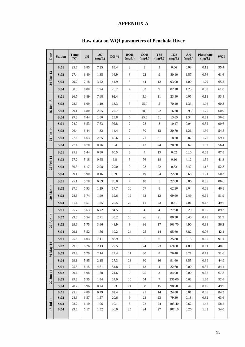
95
APPENDIX A
Raw data on WQI parameters of Penchala River
D
ate
Station Temp
(°C) pH
DO
(mg/L) DO %
BOD
(mg/L)
COD
(mg/L)
TSS
(mg/L)
TDS
(mg/L)
AN
(mg/L)
Phosphate
(mg/L) WQI
24
-No
v-1
3
St01 25.6 6.85 7.25 89.4 2 3 5 0.06 0.03 0.12 95.4
St02 27.4 6.40 1.35 16.9 3 22 9 80.10 1.57 0.56 61.6
St03 29.2 7.18 3.22 41.9 5 44 12 93.00 1.00 1.29 65.2
St04 30.5 6.80 1.94 25.7 4 33 9 82.10 1.25 0.58 61.8
16
-Dec
-13
St01 26.5 6.89 7.68 92.4 4 5.0 11 23.40 0.05 0.11 93.8
St02 28.9 6.69 1.10 13.3 5 25.0 5 70.10 1.33 1.06 60.3
St03 29.1 6.80 2.05 27.7 5 38.0 22 16.20 0.95 1.25 60.9
St04 29.3 7.44 1.60 19.8 6 25.0 51 13.65 1.34 0.81 56.6
24
-Ja
n-1
4
St01 24.7 6.53 7.63 92.8 2 28 8 10.17 0.04 0.32 90.6
St02 26.4 6.44 1.32 14.4 7 50 13 20.70 1.26 1.60 54.5
St03 27.6 6.63 2.65 40.6 7 71 31 18.70 0.87 1.76 59.1
St04 27.4 6.70 0.26 3.4 7 42 24 20.30 0.62 1.32 56.4
25
-Feb
-14
St01 25.9 5.44 6.80 80.5 3 4 13 0.02 0.10 0.08 87.8
St02 27.2 5.18 0.65 6.8 5 76 18 0.10 4.12 1.59 41.3
St03 30.3 6.17 2.08 29.0 9 28 22 0.33 3.42 1.17 52.8
St04 29.1 5.90 0.16 0.9 7 19 24 22.80 3.68 1.21 50.3
30
-Ma
r-1
4
St01 25.1 5.70 6.59 78.0 4 18 5 22.80 0.06 0.05 86.6
St02 27.6 5.93 1.19 17.7 10 57 8 62.30 3.04 0.68 46.8
St03 28.8 5.74 1.90 39.6 19 32 12 69.60 2.49 0.55 51.9
St04 31.4 5.51 1.85 25.5 25 11 23 0.31 2.01 0.47 49.6
29
-Ap
r-1
4
St01 25.7 5.63 6.72 84.5 3 4 4 27.90 0.20 0.06 89.3
St02 29.6 5.54 2.71 35.2 10 26 21 80.30 6.40 0.78 51.9
St03 29.6 5.75 3.66 48.9 9 36 17 103.70 4.90 0.93 56.2
St04 29.1 5.52 1.56 19.2 24 25 14 95.60 3.82 0.76 42.4
30
-May
-14
St01 25.8 6.03 7.11 86.9 3 5 6 25.80 0.15 0.05 91.1
St02 29.8 5.26 2.13 27.5 9 24 23 69.80 4.80 0.61 48.6
St03 29.9 5.79 2.14 27.4 11 30 8 76.40 3.21 0.72 51.6
St04 29.1 5.85 2.15 27.3 23 30 16 91.60 3.55 0.39 44.9
27
-Ju
n-1
4
St01 25.5 6.15 4.61 54.8 2 13 4 22.60 0.00 0.35 84.1
St02 29.4 5.98 1.88 24.6 9 25 3 84.00 0.00 0.82 67.8
St03 29.3 5.35 1.84 24.0 10 64 7 235.00 0.62 1.30 52.6
St04 28.7 5.96 0.24 3.3 21 38 15 98.70 0.44 0.46 49.9
15
-Ju
l-1
4
St01 25.3 4.89 6.79 82.4 3 21 14 24.80 0.01 0.06 84.3
St02 28.6 6.57 1.57 20.6 9 23 23 79.30 0.18 0.82 63.6
St03 28.7 6.10 1.06 10.1 8 22 24 105.40 0.62 1.42 58.2
St04
29.6 5.17 1.52 36.0 25 24 27 107.10 0.26 1.02 54.0

96
Da
te
Station Temp
(°C) pH
DO
(mg/L) DO %
BOD
(mg/L)
COD
(mg/L)
TSS
(mg/L)
TDS
(mg/L)
AN
(mg/L)
Phosphate
(mg/L) WQI
29
-Au
g-1
4 St01 25.5 6.82 6.55 79.6 3 21 3 24.00 0.01 0.61 90.0
St02 28.4 6.23 1.55 20.1 12 81 18 80.40 0.24 0.47 53.5
St03 28.9 5.39 1.62 21.0 10 57 59 117.40 1.23 1.63 46.2
St04 28.5 5.45 0.32 4.1 20 73 7 108.60 0.42 1.32 44.8
19
-Sep
-14 St01 24.7 6.15 3.03 53.8 0 15 4 33.62 0.06 0.22 84.1
St02 29.9 6.02 2.88 55.9 11 30 70 71.20 1.66 1.46 60.2
St03 25.1 6.32 2.08 40.6 13 45 9 100.70 3.36 1.14 52.8
St04 28.8 5.92 2.41 47.4 22 60 7 72.60 3.06 0.72 49.3
25
-Oct-
14 St01 25.7 6.03 3.40 60.3 2 30 13 17.52 0.04 0.21 81.8
St02 28.9 5.78 2.27 42.9 5 60 9 55.20 3.64 0.40 55.6
St03 28.9 5.72 2.10 39.8 15 64 7 70.80 2.02 1.06 51.5
St04 27.9 5.77 1.65 30.8 12 45 8 67.40 2.62 0.34 51.2

97
APPENDIX B
Raw data on physical parameters of Penchala River
Date Station Water
Level (m)
River
width (m)
Area
(m²) N
No. Rev(n) @ Time(T),
Distance D)
Velocity, v
(m/s)
Discharge,
Q (m3s-1) 2
4-N
ov
-13 St01 0.10 0.47 0.0470 4.511 0.4898 0.023021
St02 0.15 14.30 2.1450 2.042 0.2376 0.509652
St03 0.47 13.00 6.1100 D=9.6m , T=17.69s 0.3841 2.346851
St04 0.52 25.00 13.0000 D=8.0m , T=38.47s 0.3017 3.922100
16
-Dec
-13 St01 0.18 0.50 0.0900 5.482 0.1527 0.013743
St02 0.21 14.30 3.0030 2.232 0.2582 0.775375
St03 0.45 13.00 5.8500 3.41 0.4486 2.624310
St04 0.81 25.00 20.2500 2.192 0.2544 5.151600
24
-Ja
n-1
4 St01 0.06 0.68 0.0408 4.358 0.4697 0.019164
St02 0.45 14.30 6.4350 5.327 0.5710 3.674385
St03 0.36 13.00 4.6800 1.718 0.1914 0.895752
St04 1.84 25.00 46.0000 D=5.0m , T=39.22s 0.1355 6.233000
25
-Feb
-14 St01 0.08 0.53 0.0398 2.49 0.2819 0.011206
St02 0.30 14.30 4.2900 1.282 0.1567 0.672243
St03 0.30 13.00 3.9000 1.533 0.1876 0.731640
St04 2.23 25.00 55.7500 D= 4.70m , T=33.91s 0.1363 7.598725
30
-Ma
r-1
4 St01 0.07 0.86 0.0602 77.60 2.59 0.2914 0.017542
St02 0.30 14.30 4.2900 40.00 1.333 0.1621 0.695409
St03 0.30 13.00 3.9000 53.85 1.795 0.3000 1.170000
St04 0.30 25.00 7.5000 D=1.1m , T=10.21s 0.3000 2.250000
29
-Ap
r-1
4 St01 0.10 0.60 0.0600 208.60 2.59 0.2928 0.017568
St02 0.47 14.30 6.7210 35.50 1.333 0.1701 1.143242
St03 0.47 13.00 6.1100 115.85 1.795 0.4700 2.871700
St04 0.47 25.00 11.7500 D=1.1m , T=10.21s 0.4000 4.700000
25
-May
-14 St01 0.11 2.00 0.2200 163.50 0.2669 0.058718
St02 0.48 14.30 6.8640 30.15 0.1788 1.227283
St03 0.37 13.00 4.8100 77.40 0.2960 1.423760
St04 0.60 25.00 15.0000 30.60 D=1.1m , T=25.7s 0.1385 2.077500
25
-Ju
n-1
4 St01 0.60 1.62 0.9720 D= 1m , T= 4 s 0.2925 0.284310
St02 0.44 14.30 6.2920 D= 6.1m , T= 17.6 s 0.3601 2.265749
St03 0.44 13.00 5.7200 D= 9.6m , T= 17.5 s 0.4400 2.516800
St04 0.44 25.00 11.0000 D= 1.1m , T= 11.6 s 0.4400 4.840000
15
-Ju
l-1
4 St01 0.06 1.32 0.0792 116.35 3.8783 0.4142 0.032805
St02 0.50 14.30 7.1500 D= 5.6m , T= 17.52 s 0.3107 2.221505
St03 0.35 13.00 4.5500 67.90 2.2633 0.2589 1.177995
St04 0.50 25.00 12.5000 D= 8.812m , T= 23.15 s 0.3610 4.512500
29
-Au
g-1
4 St01 0.06 0.77 0.0431 88.40 2.94667 0.3402 0.014669
St02 0.45 14.30 6.4350 D= 3.352m , T= 7.70 s 0.4169 2.682752
St03 0.31 13.00 4.0300 70.45 2.345833 0.2889 1.164267
St04 0.40 25.00 10.0000 D= 8.7m , T= 14.65 s 0.5930 5.930000
25
-Sep
-14 St01 0.34 6.00 2.0400 0 0.1815 0.370260
St02 0.48 14.30 6.8640 D= 13.73m , T= 7.162 s 1.9419 13.329202
St03 0.35 13.00 4.5500 82.43 2.74767 0.3050 1.387545
St04 0.60 25.00 15.0000 D= 7.25m , T= 17.20 s 0.4215 6.322500
25
-Oct-
14 St01 0.26 6.27 1.6302 0.0821 0.133839
St02 0.45 14.30 6.4350 0.6553 4.216856
St03 0.39 13.00 5.0700 0.3205 1.625112
St04 0.54 25.00 13.5000 2.1743 29.352600