9/19/2016 1

Physics 2310 Lab #3 Driven Harmonic Oscillator

M. Pierce (adapted from a lab by the UCLA Physics & Astronomy Department)

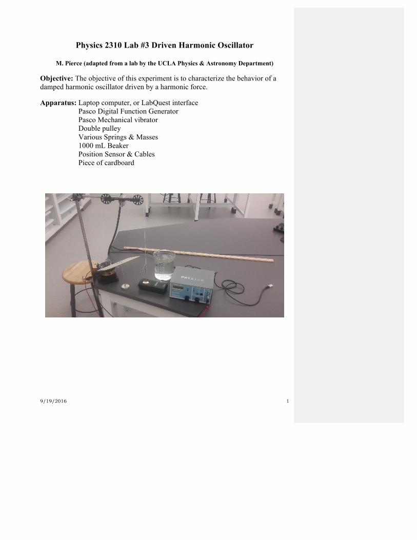
Objective: The objective of this experiment is to characterize the behavior of a damped harmonic oscillator driven by a harmonic force. Apparatus: Laptop computer, or LabQuest interface

Pasco Digital Function Generator Pasco Mechanical vibrator

Double pulley Various Springs & Masses 1000 mL Beaker Position Sensor & Cables Piece of cardboard

9/19/2016 2

Theory: Hooke's Law for a mass attached to a spring states that Fs = -kx, where x is the displacement of the mass from equilibrium, F is the restoring force exerted by the spring on the mass, and k is the (positive) spring constant. If this force causes the mass m to accelerate, then the equation of motion for the mass is −kx = ma. (1) Substituting for the acceleration a = d2x/dt2, we can rewrite Eq. (1) as: −kx = md2x/dt2 (2) or: d2x/dt2 + w2

0x = 0, (3) where ω0 = √k/m is called the resonance angular frequency of oscillation. Eq. (3) is the differential equation for a simple harmonic oscillator with no friction. Its solution includes the sine and cosine functions, since the second derivatives of these functions are proportional to the negatives of the functions. Thus, the solution x(t) = Asin(ω0t) + Bcos(ω0t) satisfies Eq. 3. The parameters A and B are two constants, which can be determined by the initial conditions of the motion. The natural frequency f0 of such an oscillator is:

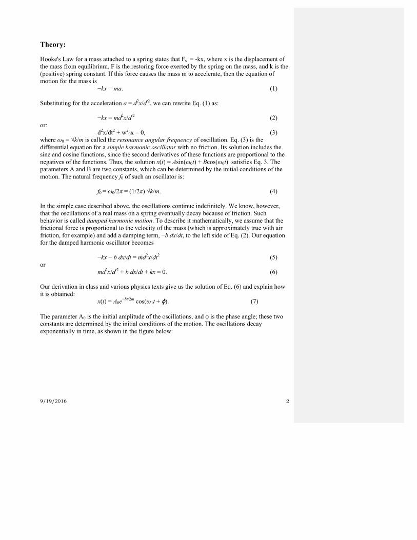
f0 = ω0/2π = (1/2π) √k/m. (4) In the simple case described above, the oscillations continue indefinitely. We know, however, that the oscillations of a real mass on a spring eventually decay because of friction. Such behavior is called damped harmonic motion. To describe it mathematically, we assume that the frictional force is proportional to the velocity of the mass (which is approximately true with air friction, for example) and add a damping term, −b dx/dt, to the left side of Eq. (2). Our equation for the damped harmonic oscillator becomes −kx − b dx/dt = md2x/dt2 (5) or md2x/dt2 + b dx/dt + kx = 0. (6) Our derivation in class and various physics texts give us the solution of Eq. (6) and explain how it is obtained: x(t) = A0e−bt/2m cos(ω1t + ϕ). (7) The parameter A0 is the initial amplitude of the oscillations, and φ is the phase angle; these two constants are determined by the initial conditions of the motion. The oscillations decay exponentially in time, as shown in the figure below:

9/19/2016 3

Figure 1: The expected amplitude vs. time for a harmonic oscillator with damping. ω1 = √k/m − (b/2m)2 = √ ω2

0− (b/2m) ω20. (8)

Now imagine that an external force which varies sinusoidally in time is applied to the mass at an arbitrary angular frequency ω. The resultant behavior of the mass is known as driven harmonic motion. The mass vibrates with a relatively small amplitude, unless the driving angular frequency is near the resonance angular frequency ωo. In this case, the amplitude becomes very large. If the external force has the form Fm cos(ω2t), then our equation for the driven harmonic oscillator can be written as −kx − b dx/dt + Fm cos(ω2t) = md2x/dt2 (9) or md2x/dt2 + b dx/dt + kx = Fm cos(ω2t). (10) The solution of Eq. (10) was derived in class and can also be found in physics texts: x(t) = (Fm/G) cos(ω2t + ϕ), (11) where: G = √ (m2 ω2

2- ω20)2 +b2ω2

2 and

ϕ = cos−1(bω2/G). The factor in the denominator of Eq. (11), G, determines the shape of the resonance curve, which we wish to measure in this experiment. When the driving angular frequency ω2 is close to the resonance angular frequency ω0, is small, and the amplitude of oscillation becomes large. When the driving angular frequency is far from the resonance angular frequency ω0, G is large, and the amplitude of oscillation is small

9/19/2016 4

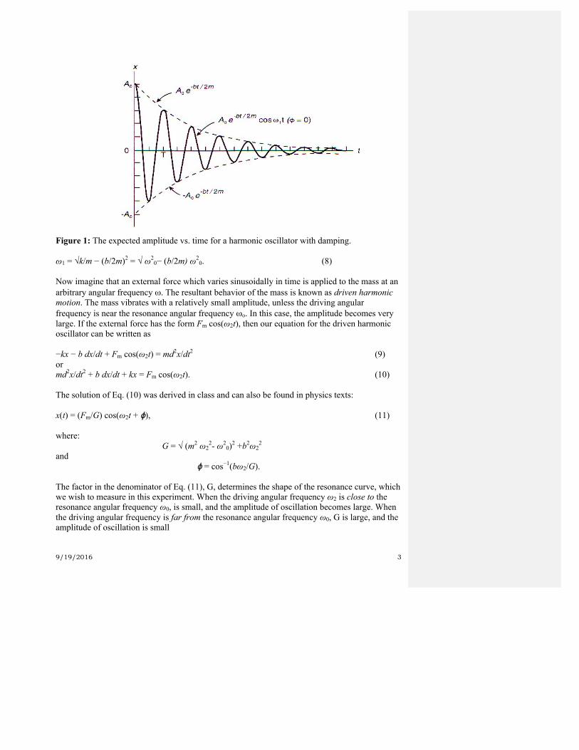
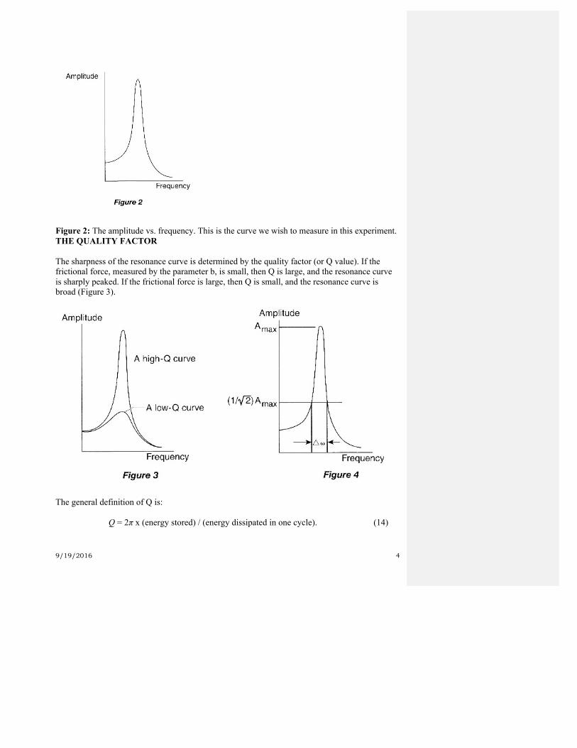
Figure 2: The amplitude vs. frequency. This is the curve we wish to measure in this experiment. THE QUALITY FACTOR The sharpness of the resonance curve is determined by the quality factor (or Q value). If the frictional force, measured by the parameter b, is small, then Q is large, and the resonance curve is sharply peaked. If the frictional force is large, then Q is small, and the resonance curve is broad (Figure 3).

The general definition of Q is:

Q = 2π x (energy stored) / (energy dissipated in one cycle). (14)

9/19/2016 5

(If the energy dissipated per cycle is small, then Q is large, and the resonance curve is sharply peaked.) In class we derived the relationship between Q and the motion parameters,

Q = mω1/b, (15) and related Q to the sharpness of the resonance peak,

Q = ω1/Δω, (16) where Δω = ωhigh - ωlow is the difference in angular frequencies at which the amplitude has dropped to 1/√ 2 of its maximum value (see Figure 4). Note that Q also controls the exponential damping factor, e−bt/2m, in Eq. (7) and Figure 1. Using Eq. (15), it is clear that

e−bt/2m = e−ω1t/2Q. (17) The reciprocal of the factor which multiplies in the exponent, 2m/b = 2Q/ ω1, is the time required for the amplitude of oscillation to decay to e-1 of its initial value (the so-called “e-folding time”). EXPERIMENTAL SETUP There are two sets of software that can be used for this lab. The first way is to use a computer equipped with the LoggerPro software. The second way is to use a handheld with LabQuest. The following directions will be generalized but will include specific directions for each method when the process is substantially different. This experiment utilizes a signal generator, which drives a mechanical vibrator attached to a spring with a mass. We will measure the position of the mass using the ultra-sonic motion sensor (Motion Detector 2). Be careful not to put too much mass on the springs because it will permanently stretch the spring. What do you see? PROCEDURE PART 1: FINDING THE NATURAL FREQUENCY 1. Remove the spring and mass holder from the string and weigh them. Record the mass. Now

determine the spring constant. To do this start with finding the equilibrium position of the spring with the mass holder attached. Place the cardboard on the mass holder to use as an indicator and mark its position on a piece of paper. Now add some mass to the mass holder and mark the position again. Use a ruler to measure the change in the height of the cardboard and use this to measure the spring constant (k = Force applied/ distance stretched [N/m]). When finished, place the motion sensor on the table under the mass-spring system.

In the following procedures, be very careful not to drop masses onto the motion sensor. Secure the spring firmly to the vibrator stem. If the vibrations become large, they might shake a mass loose.

SA496 � 9/18/2016 4:04 PMComment [1]: Added this, but I don’t know if it is necessary.

9/19/2016 6

2. Verify that the cable from the motion sensor is plugged into digital channel 1 (DIG1) of the Lab Quest Mini (LQM) and make sure the LQM is plugged into either a computer or a LabQues Pro (LQP).

3. Position the sensor underneath the cardboard and set the mass in motion by gently pulling it down and releasing it. Verify that the oscillations are fairly uniform and that the cardboard sheet doesn’t rotate away from its position above the sensor. The cardboard also needs to be level so you get good data. If you are having trouble, then stop the oscillations and start them again a little more carefully.

4. To collect data on with LoggerPro there is a green arrow in the top center part of the screen that will start collecting data, or you can start and stop it by pressing the space bar. For the LQP pull out the stylus on the LQP. On the LQP interface, locate the green arrow at the lower left part of the screen. Touch this with the stylus when you want to collect data. Start the mass going again if necessary and Click the arrow to collect data. You will hear the range finder taking data for about 5 seconds while the position and velocity of the mass are plotted within the graphics windows.

5. Next we will set up the software to give us a frequency versus amplitude plot in order to determine the natural frequency. For LoggerPro: Go to insert, additional graphs, FFT graph. For the LQP: Under the “Analyze” menu select “Advanced” and the select the Fast Fourier Transform. On the “Insert” menu select “Additional Graphs”, select “FFT” and then “Position”. This will perform an FFT on the position vs. time and display the amplitude vs. frequency. You should see a nice well-defined peak. Clicking on the peak will give you the frequency and the amplitude of the oscillations in meters. Once you get the hang of it use this procedure to measure the frequency five times, recording them and the average below. This is the natural frequency that for the mass/spring combination. Note that the amplitude for this part doesn’t matter since it depends on how far you pull down the mass. Take a picture of the FFT graph with your smart phone or save it to a flash drive

6. Now compare the natural frequency you measured to the expected value from the mass and

spring constant that you measured (Eq. 4). How well do they agree? DATA Procedure Part 1: Mass of spring and weights = ___________________ Frequency (Trial 1) = _________________________ Frequency (Trial 2) = _________________________ Frequency (Trial 3) = _________________________ Frequency (Trial 4) = _________________________

9/19/2016 7

Frequency (Trial 5) = _________________________ Average frequency = __________________________ PROCEDURE PART 2: PLOTTING THE RESONANCE CURVE In this section, you will verify that a mechanical resonance occurs when a driving force is applied to the system with a frequency equal to the natural frequency of the oscillator.

1. Fill the beaker with water. Hang the weight hanger so it is submerged in the water to about the 800 mL mark. Turn on the signal generator. Be sure that the amplitude on the signal generator is all the way down.

2. Set the signal generator frequency to about .25 Hz and slowly turn up the amplitude until you see the mechanical vibrator begin to move.

Note that a sine wave is now driving the spring by pulling on the string. The weights hanging from the spring will respond too and oscillate up and down in the water. The water acts to provide resistance.

3. Note further that if the frequency is low the spring doesn’t stretch and the mass just moves up and down in response to the mechanical vibrator. Try slowly turning up the frequency while watching the mass in the water and the spring. Note that as the frequency increases the amplitude does as well and the mass move up down with a higher amplitude. Look at spring and note what you see. Continue increasing the frequency of the driving signal and watch the mass and spring.

4. Hang the piece of cardboard at the top part of the weight hanger and position the motion sensor so that it is below the cardboard sheet. Set the frequency of the signal generator to about 0.5 Hz (note: here you can turn up the amplitude of the frequency generator but be careful not to let the mass hanger hit the bottom or sides of the glass beaker). The mass should now be oscillating in the water within the beaker.

5. Record data the same way as in procedure 1 using a FFT graph. Start a data table for amplitude vs. frequency, paper is OK for now but be sure to share the data so everyone can enter it into Excel later.

6. Take all your measurements at the same driving amplitude so don’t adjust that. Repeat step #2 and frequency intervals that bracket the natural frequency you got in part 1. I would like to see at least 25 measurements so your frequency increment should be about 0.1 Hz.

9/19/2016 8

DATA Procedure Part 2: Amplitude at Maximum= ______________________ Frequency at Maximum Amplitude = ________________________ Enter the resonance data into an Excel spreadsheet and plot the resonance curve. Remember to label the axes and title the graph. Post-lab Questions We saw that Q = ω1/Δω, (16) where Δω = ωhigh − ωlow. Compute the value of Q for your mass on a spring by finding the angular frequencies on your resonance curve where the amplitude has dropped to about 1/√ 2 of its maximum value. Q is also equal to mω1/b, by Eq. (15). By approximating ω1 as ω0, estimate the value of b. Then compute the true resonance angular frequency, including friction, from ω1 = √k/m − (b/2m)2 . What is the percentage difference between ω1 and ω0? Could your measurements of the resonance curve have distinguished between ω1 and ω2? ωhigh = ________________ ωlow = ________________ Q = __________________ b = ___________________ ω1 = __________________ Percentage difference between ω1 and ω2 = _________________________

SA496 � 9/18/2016 6:36 PMComment [2]: This was extra credit, but I think that the students should do this so I am making it required.