physics-based deep learning
TRANSCRIPT

Physics-based Deep Learning
http://physicsbaseddeeplearning.org
N. Thuerey, P. Holl, M. Mueller, P. Schnell, F. Trost, K. Um
i
arX
iv:2
109.
0523
7v1
[cs
.LG
] 1
1 Se
p 20
21

ii

CONTENTS
I Introduction 3
1 A Teaser Example 51.1 Differentiable physics . . . . . . . . . . . . . . . . . . . . . . . . . . . . . . . . . . . . . . . . 51.2 Finding the inverse function of a parabola . . . . . . . . . . . . . . . . . . . . . . . . . . . . . 61.3 A differentiable physics approach . . . . . . . . . . . . . . . . . . . . . . . . . . . . . . . . . . 81.4 Discussion . . . . . . . . . . . . . . . . . . . . . . . . . . . . . . . . . . . . . . . . . . . . . . 111.5 Next steps . . . . . . . . . . . . . . . . . . . . . . . . . . . . . . . . . . . . . . . . . . . . . . 11
2 Overview 132.1 Motivation . . . . . . . . . . . . . . . . . . . . . . . . . . . . . . . . . . . . . . . . . . . . . . 132.2 Categorization . . . . . . . . . . . . . . . . . . . . . . . . . . . . . . . . . . . . . . . . . . . . 152.3 Looking ahead . . . . . . . . . . . . . . . . . . . . . . . . . . . . . . . . . . . . . . . . . . . . 162.4 Implementations . . . . . . . . . . . . . . . . . . . . . . . . . . . . . . . . . . . . . . . . . . . 162.5 Models and Equations . . . . . . . . . . . . . . . . . . . . . . . . . . . . . . . . . . . . . . . . 172.6 Simple Forward Simulation of Burgers Equation with phiflow . . . . . . . . . . . . . . . . . . 202.7 Navier-Stokes Forward Simulation . . . . . . . . . . . . . . . . . . . . . . . . . . . . . . . . . 24
3 Supervised Training 313.1 Problem setting . . . . . . . . . . . . . . . . . . . . . . . . . . . . . . . . . . . . . . . . . . . 313.2 Surrogate models . . . . . . . . . . . . . . . . . . . . . . . . . . . . . . . . . . . . . . . . . . 323.3 Show me some code! . . . . . . . . . . . . . . . . . . . . . . . . . . . . . . . . . . . . . . . . . 323.4 Supervised training for RANS flows around airfoils . . . . . . . . . . . . . . . . . . . . . . . . 323.5 Discussion of Supervised Approaches . . . . . . . . . . . . . . . . . . . . . . . . . . . . . . . 45
II Physical Losses 49
4 Physical Loss Terms 514.1 Using physical models . . . . . . . . . . . . . . . . . . . . . . . . . . . . . . . . . . . . . . . . 514.2 Neural network derivatives . . . . . . . . . . . . . . . . . . . . . . . . . . . . . . . . . . . . . 524.3 Summary so far . . . . . . . . . . . . . . . . . . . . . . . . . . . . . . . . . . . . . . . . . . . 53
5 Burgers Optimization with a Physics-Informed NN 555.1 Formulation . . . . . . . . . . . . . . . . . . . . . . . . . . . . . . . . . . . . . . . . . . . . . 555.2 Preliminaries . . . . . . . . . . . . . . . . . . . . . . . . . . . . . . . . . . . . . . . . . . . . . 565.3 Loss function and training . . . . . . . . . . . . . . . . . . . . . . . . . . . . . . . . . . . . . 585.4 Evaluation . . . . . . . . . . . . . . . . . . . . . . . . . . . . . . . . . . . . . . . . . . . . . . 605.5 Next steps . . . . . . . . . . . . . . . . . . . . . . . . . . . . . . . . . . . . . . . . . . . . . . 66
6 Discussion of Physical Soft-Constraints 676.1 Is it “Machine Learning”? . . . . . . . . . . . . . . . . . . . . . . . . . . . . . . . . . . . . . . 67
iii

6.2 Summary . . . . . . . . . . . . . . . . . . . . . . . . . . . . . . . . . . . . . . . . . . . . . . . 68
III Differentiable Physics 69
7 Introduction to Differentiable Physics 717.1 Differentiable operators . . . . . . . . . . . . . . . . . . . . . . . . . . . . . . . . . . . . . . . 727.2 Jacobians . . . . . . . . . . . . . . . . . . . . . . . . . . . . . . . . . . . . . . . . . . . . . . . 727.3 Learning via DP operators . . . . . . . . . . . . . . . . . . . . . . . . . . . . . . . . . . . . . 737.4 A practical example . . . . . . . . . . . . . . . . . . . . . . . . . . . . . . . . . . . . . . . . . 747.5 Implicit gradient calculations . . . . . . . . . . . . . . . . . . . . . . . . . . . . . . . . . . . . 777.6 Summary of differentiable physics so far . . . . . . . . . . . . . . . . . . . . . . . . . . . . . . 78
8 Burgers Optimization with a Differentiable Physics Gradient 798.1 Initialization . . . . . . . . . . . . . . . . . . . . . . . . . . . . . . . . . . . . . . . . . . . . . 798.2 Gradients . . . . . . . . . . . . . . . . . . . . . . . . . . . . . . . . . . . . . . . . . . . . . . . 808.3 Optimization . . . . . . . . . . . . . . . . . . . . . . . . . . . . . . . . . . . . . . . . . . . . . 818.4 More optimization steps . . . . . . . . . . . . . . . . . . . . . . . . . . . . . . . . . . . . . . . 838.5 Physics-informed vs. differentiable physics reconstruction . . . . . . . . . . . . . . . . . . . . 868.6 Next steps . . . . . . . . . . . . . . . . . . . . . . . . . . . . . . . . . . . . . . . . . . . . . . 88
9 Discussion 899.1 Time steps and iterations . . . . . . . . . . . . . . . . . . . . . . . . . . . . . . . . . . . . . . 899.2 Alternatives: noise . . . . . . . . . . . . . . . . . . . . . . . . . . . . . . . . . . . . . . . . . . 919.3 Summary . . . . . . . . . . . . . . . . . . . . . . . . . . . . . . . . . . . . . . . . . . . . . . . 91
10 Differentiable Fluid Simulations 9310.1 Physical Model . . . . . . . . . . . . . . . . . . . . . . . . . . . . . . . . . . . . . . . . . . . . 9310.2 Formulation . . . . . . . . . . . . . . . . . . . . . . . . . . . . . . . . . . . . . . . . . . . . . 9310.3 Starting the Implementation . . . . . . . . . . . . . . . . . . . . . . . . . . . . . . . . . . . . 9410.4 Batched simulations . . . . . . . . . . . . . . . . . . . . . . . . . . . . . . . . . . . . . . . . . 9410.5 Gradients . . . . . . . . . . . . . . . . . . . . . . . . . . . . . . . . . . . . . . . . . . . . . . . 9610.6 Optimization . . . . . . . . . . . . . . . . . . . . . . . . . . . . . . . . . . . . . . . . . . . . . 9710.7 Re-simulation . . . . . . . . . . . . . . . . . . . . . . . . . . . . . . . . . . . . . . . . . . . . 9910.8 Conclusions . . . . . . . . . . . . . . . . . . . . . . . . . . . . . . . . . . . . . . . . . . . . . . 10110.9 Next steps . . . . . . . . . . . . . . . . . . . . . . . . . . . . . . . . . . . . . . . . . . . . . . 101
11 Differentiable Physics versus Physics-informed Training 10311.1 Compatibility with existing numerical methods . . . . . . . . . . . . . . . . . . . . . . . . . . 10311.2 Discretization . . . . . . . . . . . . . . . . . . . . . . . . . . . . . . . . . . . . . . . . . . . . 10311.3 Efficiency . . . . . . . . . . . . . . . . . . . . . . . . . . . . . . . . . . . . . . . . . . . . . . . 10411.4 Efficiency continued . . . . . . . . . . . . . . . . . . . . . . . . . . . . . . . . . . . . . . . . . 10411.5 Summary . . . . . . . . . . . . . . . . . . . . . . . . . . . . . . . . . . . . . . . . . . . . . . . 104
IV Complex Examples with DP 107
12 Complex Examples Overview 109
13 Reducing Numerical Errors with Deep Learning 11113.1 Problem formulation . . . . . . . . . . . . . . . . . . . . . . . . . . . . . . . . . . . . . . . . . 11113.2 Getting started with the implementation . . . . . . . . . . . . . . . . . . . . . . . . . . . . . 11213.3 Simulation setup . . . . . . . . . . . . . . . . . . . . . . . . . . . . . . . . . . . . . . . . . . . 11313.4 Network architecture . . . . . . . . . . . . . . . . . . . . . . . . . . . . . . . . . . . . . . . . 11413.5 Data handling . . . . . . . . . . . . . . . . . . . . . . . . . . . . . . . . . . . . . . . . . . . . 116
iv

13.6 Interleaving simulation and NN . . . . . . . . . . . . . . . . . . . . . . . . . . . . . . . . . . 12013.7 Training . . . . . . . . . . . . . . . . . . . . . . . . . . . . . . . . . . . . . . . . . . . . . . . 12213.8 Evaluation . . . . . . . . . . . . . . . . . . . . . . . . . . . . . . . . . . . . . . . . . . . . . . 12413.9 Next steps . . . . . . . . . . . . . . . . . . . . . . . . . . . . . . . . . . . . . . . . . . . . . . 129
14 Solving Inverse Problems with NNs 13114.1 Formulation . . . . . . . . . . . . . . . . . . . . . . . . . . . . . . . . . . . . . . . . . . . . . 13214.2 Control of incompressible fluids . . . . . . . . . . . . . . . . . . . . . . . . . . . . . . . . . . 13214.3 Data generation . . . . . . . . . . . . . . . . . . . . . . . . . . . . . . . . . . . . . . . . . . . 13314.4 Supervised initialization . . . . . . . . . . . . . . . . . . . . . . . . . . . . . . . . . . . . . . . 13514.5 CFE pretraining with differentiable physics . . . . . . . . . . . . . . . . . . . . . . . . . . . . 13614.6 End-to-end training with differentiable physics . . . . . . . . . . . . . . . . . . . . . . . . . . 13614.7 Next steps . . . . . . . . . . . . . . . . . . . . . . . . . . . . . . . . . . . . . . . . . . . . . . 139
15 Summary and Discussion 14115.1 Integration . . . . . . . . . . . . . . . . . . . . . . . . . . . . . . . . . . . . . . . . . . . . . . 14115.2 Interaction . . . . . . . . . . . . . . . . . . . . . . . . . . . . . . . . . . . . . . . . . . . . . . 14215.3 Generalization . . . . . . . . . . . . . . . . . . . . . . . . . . . . . . . . . . . . . . . . . . . . 142
V Reinforcement Learning 143
16 Introduction to Reinforcement Learning 14516.1 Algorithms . . . . . . . . . . . . . . . . . . . . . . . . . . . . . . . . . . . . . . . . . . . . . . 14616.2 Proximal policy optimization . . . . . . . . . . . . . . . . . . . . . . . . . . . . . . . . . . . . 14616.3 Application to inverse problems . . . . . . . . . . . . . . . . . . . . . . . . . . . . . . . . . . 14716.4 Implementation . . . . . . . . . . . . . . . . . . . . . . . . . . . . . . . . . . . . . . . . . . . 148
17 Controlling Burgers’ Equation with Reinforcement Learning 15117.1 Overview . . . . . . . . . . . . . . . . . . . . . . . . . . . . . . . . . . . . . . . . . . . . . . . 15117.2 Software installation . . . . . . . . . . . . . . . . . . . . . . . . . . . . . . . . . . . . . . . . . 15117.3 Data generation . . . . . . . . . . . . . . . . . . . . . . . . . . . . . . . . . . . . . . . . . . . 15217.4 Training via reinforcement learning . . . . . . . . . . . . . . . . . . . . . . . . . . . . . . . . 15317.5 RL evaluation . . . . . . . . . . . . . . . . . . . . . . . . . . . . . . . . . . . . . . . . . . . . 15617.6 Differentiable physics training . . . . . . . . . . . . . . . . . . . . . . . . . . . . . . . . . . . 15717.7 Comparison between RL and DP . . . . . . . . . . . . . . . . . . . . . . . . . . . . . . . . . . 16117.8 Training progress comparison . . . . . . . . . . . . . . . . . . . . . . . . . . . . . . . . . . . . 16517.9 Next steps . . . . . . . . . . . . . . . . . . . . . . . . . . . . . . . . . . . . . . . . . . . . . . 166
VI PBDL and Uncertainty 167
18 Introduction to Posterior Inference 16918.1 Uncertainty . . . . . . . . . . . . . . . . . . . . . . . . . . . . . . . . . . . . . . . . . . . . . . 16918.2 Introduction to Bayesian Neural Networks . . . . . . . . . . . . . . . . . . . . . . . . . . . . 17018.3 Prior distributions . . . . . . . . . . . . . . . . . . . . . . . . . . . . . . . . . . . . . . . . . . 17018.4 Evidence lower bound . . . . . . . . . . . . . . . . . . . . . . . . . . . . . . . . . . . . . . . . 17118.5 The BNN training loop . . . . . . . . . . . . . . . . . . . . . . . . . . . . . . . . . . . . . . . 17118.6 Dropout as alternative . . . . . . . . . . . . . . . . . . . . . . . . . . . . . . . . . . . . . . . 17218.7 A practical example . . . . . . . . . . . . . . . . . . . . . . . . . . . . . . . . . . . . . . . . . 172
19 RANS Airfoil Flows with Bayesian Neural Nets 17319.1 Overview . . . . . . . . . . . . . . . . . . . . . . . . . . . . . . . . . . . . . . . . . . . . . . . 17319.2 Training . . . . . . . . . . . . . . . . . . . . . . . . . . . . . . . . . . . . . . . . . . . . . . . 17919.3 Test evaluation . . . . . . . . . . . . . . . . . . . . . . . . . . . . . . . . . . . . . . . . . . . . 184
v

19.4 Next steps . . . . . . . . . . . . . . . . . . . . . . . . . . . . . . . . . . . . . . . . . . . . . . 188
VII Fast Forward Topics 189
20 Additional Topics 191
21 Model Reduction and Time Series 19321.1 Reduced order models . . . . . . . . . . . . . . . . . . . . . . . . . . . . . . . . . . . . . . . . 19421.2 Time series . . . . . . . . . . . . . . . . . . . . . . . . . . . . . . . . . . . . . . . . . . . . . . 19521.3 End-to-end training . . . . . . . . . . . . . . . . . . . . . . . . . . . . . . . . . . . . . . . . . 19521.4 Source code . . . . . . . . . . . . . . . . . . . . . . . . . . . . . . . . . . . . . . . . . . . . . . 196
22 Generative Adversarial Networks 19722.1 Maximum likelihood estimation . . . . . . . . . . . . . . . . . . . . . . . . . . . . . . . . . . 19722.2 Adversarial training . . . . . . . . . . . . . . . . . . . . . . . . . . . . . . . . . . . . . . . . . 19822.3 Regularization . . . . . . . . . . . . . . . . . . . . . . . . . . . . . . . . . . . . . . . . . . . . 19822.4 Conditional GANs . . . . . . . . . . . . . . . . . . . . . . . . . . . . . . . . . . . . . . . . . . 19922.5 Ambiguous solutions . . . . . . . . . . . . . . . . . . . . . . . . . . . . . . . . . . . . . . . . . 19922.6 Spatio-temporal super-resolution . . . . . . . . . . . . . . . . . . . . . . . . . . . . . . . . . . 19922.7 Physical generative models . . . . . . . . . . . . . . . . . . . . . . . . . . . . . . . . . . . . . 20022.8 Discussion . . . . . . . . . . . . . . . . . . . . . . . . . . . . . . . . . . . . . . . . . . . . . . 20122.9 Source code . . . . . . . . . . . . . . . . . . . . . . . . . . . . . . . . . . . . . . . . . . . . . . 201
23 Unstructured Meshes and Meshless Methods 20323.1 Types of computational meshes . . . . . . . . . . . . . . . . . . . . . . . . . . . . . . . . . . 20323.2 Unstructured meshes and graph neural networks . . . . . . . . . . . . . . . . . . . . . . . . . 20423.3 Meshless and particle-based methods . . . . . . . . . . . . . . . . . . . . . . . . . . . . . . . 20423.4 Continuous convolutions . . . . . . . . . . . . . . . . . . . . . . . . . . . . . . . . . . . . . . 20423.5 Learning the dynamics of liquids . . . . . . . . . . . . . . . . . . . . . . . . . . . . . . . . . . 20523.6 Source code . . . . . . . . . . . . . . . . . . . . . . . . . . . . . . . . . . . . . . . . . . . . . . 206
VIII End Matter 207
24 Outlook 20924.1 Some specific directions . . . . . . . . . . . . . . . . . . . . . . . . . . . . . . . . . . . . . . . 20924.2 Closing remarks . . . . . . . . . . . . . . . . . . . . . . . . . . . . . . . . . . . . . . . . . . . 210
25 Notation and Abbreviations 21125.1 Math notation: . . . . . . . . . . . . . . . . . . . . . . . . . . . . . . . . . . . . . . . . . . . . 21125.2 Summary of the most important abbreviations: . . . . . . . . . . . . . . . . . . . . . . . . . . 211
Bibliography 213
vi
Physics-based Deep Learning
Welcome to the Physics-based Deep Learning Book (v0.1)
TL;DR: This document contains a practical and comprehensive introduction of everything related to deeplearning in the context of physical simulations. As much as possible, all topics come with hands-on codeexamples in the form of Jupyter notebooks to quickly get started. Beyond standard supervised learning fromdata, we’ll look at physical loss constraints, more tightly coupled learning algorithms with differentiablesimulations, as well as reinforcement learning and uncertainty modeling. We live in exciting times: thesemethods have a huge potential to fundamentally change what computer simulations can achieve.
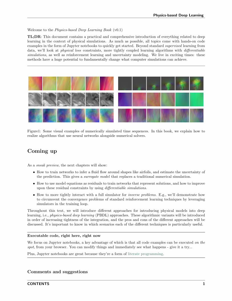
Figure1: Some visual examples of numerically simulated time sequences. In this book, we explain how torealize algorithms that use neural networks alongside numerical solvers.
Coming up
As a sneak preview, the next chapters will show:
• How to train networks to infer a fluid flow around shapes like airfoils, and estimate the uncertainty ofthe prediction. This gives a surrogate model that replaces a traditional numerical simulation.
• How to use model equations as residuals to train networks that represent solutions, and how to improveupon these residual constraints by using differentiable simulations.
• How to more tightly interact with a full simulator for inverse problems. E.g., we’ll demonstrate howto circumvent the convergence problems of standard reinforcement learning techniques by leveragingsimulators in the training loop.
Throughout this text, we will introduce different approaches for introducing physical models into deeplearning, i.e., physics-based deep learning (PBDL) approaches. These algorithmic variants will be introducedin order of increasing tightness of the integration, and the pros and cons of the different approaches will bediscussed. It’s important to know in which scenarios each of the different techniques is particularly useful.
Executable code, right here, right now
We focus on Jupyter notebooks, a key advantage of which is that all code examples can be executed on thespot, from your browser. You can modify things and immediately see what happens - give it a try...
Plus, Jupyter notebooks are great because they’re a form of literate programming.
Comments and suggestions
CONTENTS 1

Physics-based Deep Learning
This book, where “book” stands for a collection of digital texts and code examples, is maintained by the TUMPhysics-based Simulation Group. Feel free to contact us if you have any comments, e.g., via old fashionedemail. If you find mistakes, please also let us know! We’re aware that this document is far from perfect, andwe’re eager to improve it. Thanks in advance ! Btw., we also maintain a link collection with recent researchpapers.
Thanks!
This project would not have been possible without the help of many people who contributed. Thanks toeveryone Here’s an alphabetical list:
• Philipp Holl
• Maximilian Mueller
• Patrick Schnell
• Felix Trost
• Nils Thuerey
• Kiwon Um
Additional thanks go to Georg Kohl for the nice divider images (cf. [KUT20]), Li-Wei Chen for the airfoildata image, and to Chloe Paillard for proofreading parts of the document.
Citation
If you find this book useful, please cite it via:
@bookthuerey2021pbdl,
title=Physics-based Deep Learning,
author=Nils Thuerey and Philipp Holl and Maximilian Mueller and Patrick Schnell and Felix Trost
→˓and Kiwon Um,
url=https://physicsbaseddeeplearning.org,
year=2021,
publisher=WWW
2 CONTENTS
Part I
Introduction
3


CHAPTER
ONE
A TEASER EXAMPLE
Let’s start with a very reduced example that highlights some of the key capabilities of physics-based learningapproaches. Let’s assume our physical model is a very simple equation: a parabola along the positive x-axis.
Despite being very simple, for every point along there are two solutions, i.e. we have two modes, one abovethe other one below the x-axis, as shown on the left below. If we don’t take care a conventional learningapproach will give us an approximation like the red one shown in the middle, which is completely off. With animproved learning setup, ideally, by using a discretized numerical solver, we can at least accurately representone of the modes of the solution (shown in green on the right).
Figure1: Side by side - supervised versus differentiable physics training.
1.1 Differentiable physics
One of the key concepts of the following chapters is what we’ll call differentiable physics (DP). This meansthat we use domain knowledge in the form of model equations, and then integrate discretized versions ofthese models into the training process. As implied by the name, having differentiable formulations is crucialfor this process to support the training of neural networks.
Let’s illustrate the properties of deep learning via DP with the following example: We’d like to find anunknown function 𝑓* that generates solutions from a space 𝑌 , taking inputs from 𝑋, i.e. 𝑓* : 𝑋 → 𝑌 . Inthe following, we’ll often denote idealized, and unknown functions with a * superscript, in contrast to theirdiscretized, realizable counterparts without this superscript.
Let’s additionally assume we have a generic differential equation 𝒫* : 𝑌 → 𝑍 (our model equation), thatencodes a property of the solutions, e.g. some real world behavior we’d like to match. Later on, 𝑃 * willoften represent time evolutions, but it could also be a constraint for conservation of mass (then 𝒫* wouldmeasure divergence). But to keep things as simple as possible here, the model we’ll look at in the followingis a mapping back to the input space 𝑋, i.e. 𝒫* : 𝑌 → 𝑋.
Using a neural network 𝑓 to learn the unknown and ideal function 𝑓*, we could turn to classic supervisedtraining to obtain 𝑓 by collecting data. This classical setup requires a dataset by sampling 𝑥 from 𝑋 and
5

Physics-based Deep Learning
adding the corresponding solutions 𝑦 from 𝑌 . We could obtain these, e.g., by classical numerical techniques.Then we train the NN 𝑓 in the usual way using this dataset.
In contrast to this supervised approach, employing a differentiable physics approach takes advantage of thefact that we can often use a discretized version of the physical model 𝒫 and employ it to guide the trainingof 𝑓 . I.e., we want 𝑓 to be aware of our simulator 𝒫, and to interact with it. This can vastly improve thelearning, as we’ll illustrate below with a very simple example (more complex ones will follow later on).
Note that in order for the DP approach to work, 𝒫 has to be differentiable, as implied by the name. Thesedifferentials, in the form of a gradient, are what’s driving the learning process.
1.2 Finding the inverse function of a parabola
To illustrate the difference of supervised and DP approaches, we consider the following simplified setting:Given the function 𝒫 : 𝑦 → 𝑦2 for 𝑦 in the interval [0, 1], find the unknown function 𝑓 such that 𝒫(𝑓(𝑥)) = 𝑥for all 𝑥 in [0, 1]. Note: to make things a bit more interesting, we’re using 𝑦2 here for 𝒫 instead of the morecommon 𝑥2 parabola, and the discretization is simply given by representing the 𝑥 and 𝑦 via floating pointnumbers in the computer for this simple case.
We know that possible solutions for 𝑓 are the positive or negative square root function (for completeness:piecewise combinations would also be possible). Knowing that this is not overly difficult, a solution thatsuggests itself is to train a neural network to approximate this inverse mapping 𝑓 . Doing this in the “classical”supervised manner, i.e. purely based on data, is an obvious starting point. After all, this approach was shownto be a powerful tool for a variety of other applications, e.g., in computer vision.
import numpy as np
import tensorflow as tf
import matplotlib.pyplot as plt
For supervised training, we can employ our solver 𝒫 for the problem to pre-compute the solutions we needfor training: We randomly choose between the positive and the negative square root. This resembles thegeneral case, where we would gather all data available to us (e.g., using optimization techniques to computethe solutions). Such data collection typically does not favor one particular mode from multimodal solutions.
# X-Data
N = 200
X = np.random.random(N)
# Generation Y-Data
sign = (- np.ones((N,)))**np.random.randint(2,size=N)
Y = np.sqrt(X) * sign
Now we can define a network, the loss, and the training configuration. We’ll use a simple keras architecturewith three hidden layers, ReLU activations.
# Neural network
act = tf.keras.layers.ReLU()
nn_sv = tf.keras.models.Sequential([
tf.keras.layers.Dense(10, activation=act),
tf.keras.layers.Dense(10, activation=act),
tf.keras.layers.Dense(1,activation='linear')])
And we can start training via a simple mean squared error loss, using fit function from keras:
6 Chapter 1. A Teaser Example

Physics-based Deep Learning
# Loss function
loss_sv = tf.keras.losses.MeanSquaredError()
optimizer_sv = tf.keras.optimizers.Adam(lr=0.001)
nn_sv.compile(optimizer=optimizer_sv, loss=loss_sv)
# Training
results_sv = nn_sv.fit(X, Y, epochs=5, batch_size= 5, verbose=1)
Epoch 1/5
40/40 [==============================] - 0s 1ms/step - loss: 0.5084
Epoch 2/5
40/40 [==============================] - 0s 1ms/step - loss: 0.5022
Epoch 3/5
40/40 [==============================] - 0s 1ms/step - loss: 0.5011
Epoch 4/5
40/40 [==============================] - 0s 1ms/step - loss: 0.5002
Epoch 5/5
40/40 [==============================] - 0s 1ms/step - loss: 0.5007
As both NN and the data set are very small, the training converges very quickly. However, if we inspectthe predictions of the network, we can see that it is nowhere near the solution we were hoping to find: itaverages between the data points on both sides of the x-axis and therefore fails to find satisfying solutionsto the problem above.
The following plot nicely highlights this: it shows the data in light gray, and the supervised solution in red.
# Results
plt.plot(X,Y,'.',label='Data points', color="lightgray")
plt.plot(X,nn_sv.predict(X),'.',label='Supervised', color="red")
plt.xlabel('y')plt.ylabel('x')plt.title('Standard approach')plt.legend()
plt.show()
1.2. Finding the inverse function of a parabola 7

Physics-based Deep Learning
This is obviously completely wrong! The red solution is nowhere near one of the two modes of our solutionshown in gray.
Note that the red line is often not perfectly at zero, which is where the two modes of the solution shouldaverage out in the continuous setting. This is caused by the relatively coarse sampling with only 200 pointsin this example.
1.3 A differentiable physics approach
Now let’s apply a differentiable physics approach to find 𝑓 : we’ll directly include our discretized model 𝒫 inthe training.
There is no real data generation step; we only need to sample from the [0, 1] interval. We’ll simply keep thesame 𝑥 locations used in the previous case, and a new instance of a NN with the same architecture as beforenn dp:
# X-Data
# X = X , we can directly re-use the X from above, nothing has changed...
# Y is evaluated on the fly
# Model
nn_dp = tf.keras.models.Sequential([
tf.keras.layers.Dense(10, activation=act),
tf.keras.layers.Dense(10, activation=act),
tf.keras.layers.Dense(1, activation='linear')])
The loss function is the crucial point for training: we directly incorporate the function f into the loss. Inthis simple case, the loss dp function simply computes the square of the prediction y pred.
8 Chapter 1. A Teaser Example

Physics-based Deep Learning
Later on, a lot more could happen here: we could evaluate finite-difference stencils on the predicted solution,or compute a whole implicit time-integration step of a solver. Here we have a simple mean-squared errorterm of the form |𝑦2pred − 𝑦true|2, which we are minimizing during training. It’s not necessary to make it sosimple: the more knowledge and numerical methods we can incorporate, the better we can guide the trainingprocess.
#Loss
mse = tf.keras.losses.MeanSquaredError()
def loss_dp(y_true, y_pred):
return mse(y_true,y_pred**2)
optimizer_dp = tf.keras.optimizers.Adam(lr=0.001)
nn_dp.compile(optimizer=optimizer_dp, loss=loss_dp)
#Training
results_dp = nn_dp.fit(X, X, epochs=5, batch_size=5, verbose=1)
Epoch 1/5
40/40 [==============================] - 0s 656us/step - loss: 0.2814
Epoch 2/5
40/40 [==============================] - 0s 1ms/step - loss: 0.1259
Epoch 3/5
40/40 [==============================] - 0s 962us/step - loss: 0.0038
Epoch 4/5
40/40 [==============================] - 0s 949us/step - loss: 0.0014
Epoch 5/5
40/40 [==============================] - 0s 645us/step - loss: 0.0012
Now the network actually has learned a good inverse of the parabola function! The following plot shows thesolution in green.
# Results
plt.plot(X,Y,'.',label='Datapoints', color="lightgray")
#plt.plot(X,nn_sv.predict(X),'.',label='Supervised', color="red") # optional for comparison
plt.plot(X,nn_dp.predict(X),'.',label='Diff. Phys.', color="green")
plt.xlabel('x')plt.ylabel('y')plt.title('Differentiable physics approach')plt.legend()
plt.show()
1.3. A differentiable physics approach 9

Physics-based Deep Learning
This looks much better , at least in the range of 0.1 to 1.
What has happened here?
• We’ve prevented an undesired averaging of multiple modes in the solution by evaluating our discretemodel w.r.t. current prediction of the network, rather than using a pre-computed solution. This letsus find the best mode near the network prediction, and prevents an averaging of the modes that existin the solution manifold.
• We’re still only getting one side of the curve! This is to be expected because we’re representing thesolutions with a deterministic function. Hence, we can only represent a single mode. Interestingly,whether it’s the top or bottom mode is determined by the random initialization of the weights in 𝑓 -run the example a couple of times to see this effect in action. To capture multiple modes we’d needto extend the NN to capture the full distribution of the outputs and parametrize it with additionaldimensions.
• The region with 𝑥 near zero is typically still off in this example. The network essentially learns a linearapproximation of one half of the parabola here. This is partially caused by the weak neural network:it is very small and shallow. In addition, the evenly spread of sample points along the x-axis bias theNN towards the larger y values. These contribute more to the loss, and hence the network invests mostof its resources to reduce the error in this region.
10 Chapter 1. A Teaser Example

Physics-based Deep Learning
1.4 Discussion
It’s a very simple example, but it very clearly shows a failure case for supervised learning. While it mightseem very artificial at first sight, many practical PDEs exhibit a variety of these modes, and it’s often notclear where (and how many) exist in the solution manifold we’re interested in. Using supervised learning isvery dangerous in such cases. We might unknowingly get an average of these different modes.
Good and obvious examples are bifurcations in fluid flow. Smoke rising above a candle will start out straight,and then, due to tiny perturbations in its motion, start oscillating in a random direction. The images belowillustrate this case via numerical perturbations: the perfectly symmetric setup will start turning left or right,depending on how the approximation errors build up. Averaging the two modes would give an unphysical,straight flow similar to the parabola example above.
Similarly, we have different modes in many numerical solutions, and typically it’s important to recover them,rather than averaging them out. Hence, we’ll show how to leverage training via differentiable physics in thefollowing chapters for more practical and complex cases.
Figure2: A bifurcation in a buoyancy-driven fluid flow: the “smoke” shown in green color starts rising ina perfectly straight manner, but tiny numerical inaccuracies grow over time to lead to an instability withvortices alternating to one side (top-right), or in the opposite direction (bottom-right).
1.5 Next steps
For each of the following notebooks, there’s a “next steps” section like the one below which contains rec-ommendations about where to start modifying the code. After all, the whole point of these notebooks is tohave readily executable programs as a basis for own experiments. The data set and NN sizes of the examplesare often quite small to reduce the runtime of the notebooks, but they’re nonetheless good starting pointsfor potentially complex and large projects.
For the simple DP example above:
• This notebook is intentionally using a very simple setup. Change the training setup and NN above toobtain a higher-quality solution such as the green one shown in the very first image at the top.
• Or try extending the setup to a 2D case, i.e. a paraboloid. Given the function 𝒫 : (𝑦1, 𝑦2) → 𝑦21 + 𝑦22 ,find an inverse function 𝑓 such that 𝒫(𝑓(𝑥)) = 𝑥 for all 𝑥 in [0, 1].
• If you want to experiment without installing anything, you can also [run this notebook in colab].
1.4. Discussion 11

Physics-based Deep Learning
12 Chapter 1. A Teaser Example

CHAPTER
TWO
OVERVIEW
The name of this book, Physics-Based Deep Learning, denotes combinations of physical modeling and nu-merical simulations with methods based on artificial neural networks. The general direction of Physics-BasedDeep Learning represents a very active, quickly growing and exciting field of research. The following chapterwill give a more thorough introduction to the topic and establish the basics for following chapters.
Figure1: Understanding our environment, and predicting how it will evolve is one of the key challenges ofhumankind. A key tool for achieving these goals are simulations, and next-gen simulations could stronglyprofit from integrating deep learning components to make even more accurate predictions about our world.
2.1 Motivation
From weather and climate forecasts [Sto14] (see the picture above), over quantum physics [OMalleyBK+16],to the control of plasma fusion [MLA+19], using numerical analysis to obtain solutions for physical modelshas become an integral part of science.
In recent years, machine learning technologies and deep neural networks in particular, have led to impres-sive achievements in a variety of fields: from image classification [KSH12] over natural language processing[RWC+19], and more recently also for protein folding [Qur19]. The field is very vibrant and quickly devel-oping, with the promise of vast possibilities.
13

Physics-based Deep Learning
2.1.1 Replacing traditional simulations?
These success stories of deep learning (DL) approaches have given rise to concerns that this technology hasthe potential to replace the traditional, simulation-driven approach to science. E.g., recent works show thatNN-based surrogate models achieve accuracies required for real-world, industrial applications such as airfoilflows [CT21], while at the same time outperforming traditional solvers by orders of magnitude in terms ofruntime.
Instead of relying on models that are carefully crafted from first principles, can data collections of sufficientsize be processed to provide the correct answers? As we’ll show in the next chapters, this concern isunfounded. Rather, it is crucial for the next generation of simulation systems to bridge both worlds: tocombine classical numerical techniques with deep learning methods.
One central reason for the importance of this combination is that DL approaches are powerful, but atthe same time strongly profit from domain knowledge in the form of physical models. DL techniques andNNs are novel, sometimes difficult to apply, and it is admittedly often non-trivial to properly integrate ourunderstanding of physical processes into the learning algorithms.
Over the last decades, highly specialized and accurate discretization schemes have been developed to solvefundamental model equations such as the Navier-Stokes, Maxwell’s, or Schroedinger’s equations. Seeminglytrivial changes to the discretization can determine whether key phenomena are visible in the solutions or not.Rather than discarding the powerful methods that have been developed in the field of numerical mathematics,this book will show that it is highly beneficial to use them as much as possible when applying DL.
2.1.2 Black boxes and magic?
People who are unfamiliar with DL methods often associate neural networks with black boxes, and see thetraining processes as something that is beyond the grasp of human understanding. However, these viewpointstypically stem from relying on hearsay and not dealing with the topic enough.
Rather, the situation is a very common one in science: we are facing a new class of methods, and “allthe gritty details” are not yet fully worked out. However, this is pretty common for scientific advances.Numerical methods themselves are a good example. Around 1950, numerical approximations and solvershad a tough standing. E.g., to cite H. Goldstine, numerical instabilities were considered to be a “constantsource of anxiety in the future” [Gol90]. By now we have a pretty good grasp of these instabilities, andnumerical methods are ubiquitous and well established.
Thus, it is important to be aware of the fact that - in a way - there is nothing magical or otherworldly todeep learning methods. They’re simply another set of numerical tools. That being said, they’re clearly fairlynew, and right now definitely the most powerful set of tools we have for non-linear problems. Just becauseall the details aren’t fully worked out and nicely written up, that shouldn’t stop us from including thesepowerful methods in our numerical toolbox.
2.1.3 Reconciling DL and simulations
Taking a step back, the aim of this book is to build on all the powerful techniques that we have at ourdisposal for numerical simulations, and use them wherever we can in conjunction with deep learning. Assuch, a central goal is to reconcile the data-centered viewpoint with physical simulations.
Goals of this document
The key aspects that we will address in the following are:
• explain how to use deep learning techniques to solve PDE problems,
• how to combine them with existing knowledge of physics,
14 Chapter 2. Overview

Physics-based Deep Learning
• without discarding our knowledge about numerical methods.
The resulting methods have a huge potential to improve what can be done with numerical methods: in sce-narios where a solver targets cases from a certain well-defined problem domain repeatedly, it can for instancemake a lot of sense to once invest significant resources to train a neural network that supports the repeatedsolves. Based on the domain-specific specialization of this network, such a hybrid could vastly outperformtraditional, generic solvers. And despite the many open questions, first publications have demonstrated thatthis goal is not overly far away [KSA+21, UBH+20].
Another way to look at it is that all mathematical models of our nature are idealized approximations andcontain errors. A lot of effort has been made to obtain very good model equations, but to make the next bigstep forward, DL methods offer a very powerful tool to close the remaining gap towards reality [AAC+19].
2.2 Categorization
Within the area of physics-based deep learning, we can distinguish a variety of different approaches, fromtargeting constraints, combined methods, and optimizations to applications. More specifically, all approacheseither target forward simulations (predicting state or temporal evolution) or inverse problems (e.g., obtaininga parametrization for a physical system from observations).
No matter whether we’re considering forward or inverse problems, the most crucial differentiation for thefollowing topics lies in the nature of the integration between DL techniques and the domain knowledge,typically in the form of model equations via partial differential equations (PDEs). The following threecategories can be identified to roughly categorize physics-based deep learning (PBDL) techniques:
• Supervised : the data is produced by a physical system (real or simulated), but no further interactionexists. This is the classic machine learning approach.
• Loss-terms: the physical dynamics (or parts thereof) are encoded in the loss function, typically in theform of differentiable operations. The learning process can repeatedly evaluate the loss, and usuallyreceives gradients from a PDE-based formulation. These soft-constraints sometimes also go under thename “physics-informed” training.
• Interleaved : the full physical simulation is interleaved and combined with an output from a deep neuralnetwork; this requires a fully differentiable simulator and represents the tightest coupling between thephysical system and the learning process. Interleaved differentiable physics approaches are especiallyimportant for temporal evolutions, where they can yield an estimate of the future behavior of thedynamics.
2.2. Categorization 15
Physics-based Deep Learning
Thus, methods can be categorized in terms of forward versus inverse solve, and how tightly the physical modelis integrated into the optimization loop that trains the deep neural network. Here, especially interleavedapproaches that leverage differentiable physics allow for very tight integration of deep learning and numericalsimulation methods.
2.3 Looking ahead
Physical simulations are a huge field, and we won’t be able to cover all possible types of physical modelsand simulations.
Note: Rather, the focus of this book lies on:
• Field-based simulations (no Lagrangian methods)
• Combinations with deep learning (plenty of other interesting ML techniques exist, but won’t be dis-cussed here)
• Experiments are left as an outlook (i.e., replacing synthetic data with real-world observations)
It’s also worth noting that we’re starting to build the methods from some very fundamental building blocks.Here are some considerations for skipping ahead to the later chapters.
Hint: You can skip ahead if...
• you’re very familiar with numerical methods and PDE solvers, and want to get started with DL topicsright away. The Supervised Training chapter is a good starting point then.
• On the other hand, if you’re already deep into NNs&Co, and you’d like to skip ahead to the researchrelated topics, we recommend starting in the Physical Loss Terms chapter, which lays the foundationsfor the next chapters.
A brief look at our notation in the Notation and Abbreviations chapter won’t hurt in both cases, though!
2.4 Implementations
This text also represents an introduction to a wide range of deep learning and simulation APIs. We’ll usepopular deep learning APIs such as pytorch https://pytorch.org and tensorflow https://www.tensorflow.org,and additionally give introductions into the differentiable simulation framework 𝜑Flow (phiflow) https://github.com/tum-pbs/PhiFlow. Some examples also use JAX https://github.com/google/jax. Thus aftergoing through these examples, you should have a good overview of what’s available in current APIs, suchthat the best one can be selected for new tasks.
As we’re (in most Jupyter notebook examples) dealing with stochastic optimizations, many of the followingcode examples will produce slightly different results each time they’re run. This is fairly common with NNtraining, but it’s important to keep in mind when executing the code. It also means that the numbersdiscussed in the text might not exactly match the numbers you’ll see after re-running the examples.
16 Chapter 2. Overview

Physics-based Deep Learning
2.5 Models and Equations
Below we’ll give a brief (really very brief!) intro to deep learning, primarily to introduce the notation. Inaddition we’ll discuss some model equations below. Note that we’ll avoid using model to denote trainedneural networks, in contrast to some other texts and APIs. These will be called “NNs” or “networks”. A“model” will typically denote a set of model equations for a physical effect, usually PDEs.
2.5.1 Deep learning and neural networks
In this book we focus on the connection with physical models, and there are lots of great introductions todeep learning. Hence, we’ll keep it short: the goal in deep learning is to approximate an unknown function
𝑓*(𝑥) = 𝑦*, (1)
where 𝑦* denotes reference or “ground truth” solutions. 𝑓*(𝑥) should be approximated with an NN rep-resentation 𝑓(𝑥; 𝜃). We typically determine 𝑓 with the help of some variant of an error function 𝑒(𝑦, 𝑦*),where 𝑦 = 𝑓(𝑥; 𝜃) is the output of the NN. This gives a minimization problem to find 𝑓(𝑥; 𝜃) such that 𝑒 isminimized. In the simplest case, we can use an 𝐿2 error, giving
arg min𝜃|𝑓(𝑥; 𝜃) − 𝑦*|22 (2)
We typically optimize, i.e. train, with a stochastic gradient descent (SGD) optimizer of choice, e.g. Adam[KB14]. We’ll rely on auto-diff to compute the gradient w.r.t. weights, 𝜕𝑓/𝜕𝜃, We will also assume that 𝑒denotes a scalar error function (also called cost, or objective function). It is crucial for the efficient calculationof gradients that this function is scalar.
For training we distinguish: the training data set drawn from some distribution, the validation set (fromthe same distribution, but different data), and test data sets with some different distribution than thetraining one. The latter distinction is important. For the test set we want out of distribution (OOD) data tocheck how well our trained model generalizes. Note that this gives a huge range of possibilities for the testdata set: from tiny changes that will certainly work, up to completely different inputs that are essentiallyguaranteed to fail. There’s no gold standard, but test data should be generated with care.
Enough for now - if all the above wasn’t totally obvious for you, we very strongly recommend to read chapters6 to 9 of the Deep Learning book, especially the sections about MLPs and “Conv-Nets”, i.e. CNNs.
Note: Classification vs Regression
The classic ML distinction between classification and regression problems is not so important here: we onlydeal with regression problems in the following.
2.5.2 Partial differential equations as physical models
The following section will give a brief outlook for the model equations we’ll be using later on in the DLexamples. We typically target continuous PDEs denoted by 𝒫* whose solution is of interest in a spatialdomain Ω ⊂ R𝑑 in 𝑑 ∈ 1, 2, 3 dimensions. In addition, wo often consider a time evolution for a finite timeinterval 𝑡 ∈ R+. The corresponding fields are either d-dimensional vector fields, for instance u : R𝑑 ×R+ →R𝑑, or scalar p : R𝑑 × R+ → R. The components of a vector are typically denoted by 𝑥, 𝑦, 𝑧 subscripts, i.e.,v = (𝑣𝑥, 𝑣𝑦, 𝑣𝑧)𝑇 for 𝑑 = 3, while positions are denoted by x ∈ Ω.
To obtain unique solutions for 𝒫* we need to specify suitable initial conditions, typically for all quantitiesof interest at 𝑡 = 0, and boundary conditions for the boundary of Ω, denoted by Γ in the following.
2.5. Models and Equations 17

Physics-based Deep Learning
𝒫* denotes a continuous formulation, where we make mild assumptions about its continuity, we will typicallyassume that first and second derivatives exist.
We can then use numerical methods to obtain approximations of a smooth function such as 𝒫* via dis-cretization. These invariably introduce discretization errors, which we’d like to keep as small as possible.These errors can be measured in terms of the deviation from the exact analytical solution, and for discretesimulations of PDEs, they are typically expressed as a function of the truncation error 𝑂(∆𝑥𝑘), where ∆𝑥denotes the spatial step size of the discretization. Likewise, we typically have a temporal discretization viaa time step ∆𝑡.
Notation and abbreviations
If unsure, please check the summary of our mathematical notation and the abbreviations used in: Notationand Abbreviations.
We solve a discretized PDE 𝒫 by performing steps of size ∆𝑡. The solution can be expressed as a function of uand its derivatives: u(x, 𝑡+∆𝑡) = 𝒫(u𝑥,u𝑥𝑥, ...u𝑥𝑥...𝑥), where u𝑥 denotes the spatial derivatives 𝜕u(x, 𝑡)/𝜕x.
For all PDEs, we will assume non-dimensional parametrizations as outlined below, which could be re-scaledto real world quantities with suitable scaling factors. Next, we’ll give an overview of the model equations,before getting started with actual simulations and implementation examples on the next page.
2.5.3 Some example PDEs
The following PDEs are good examples, and we’ll use them later on in different settings to show how toincorporate them into DL approaches.
Burgers
We’ll often consider Burgers’ equation in 1D or 2D as a starting point. It represents a well-studied PDE,which (unlike Navier-Stokes) does not include any additional constraints such as conservation of mass. Hence,it leads to interesting shock formations. It contains an advection term (motion / transport) and a diffusionterm (dissipation due to the second law of thermodynamics). In 2D, it is given by:
𝜕𝑢𝑥
𝜕𝑡+ u · ∇𝑢𝑥 = 𝜈∇ · ∇𝑢𝑥 + 𝑔𝑥,
𝜕𝑢𝑦
𝜕𝑡+ u · ∇𝑢𝑦 = 𝜈∇ · ∇𝑢𝑦 + 𝑔𝑦 ,
(3)
where 𝜈 and g denote diffusion constant and external forces, respectively.
A simpler variant of Burgers’ equation in 1D without forces, denoting the single 1D velocity component as𝑢 = 𝑢𝑥, is given by:
𝜕𝑢
𝜕𝑡+ 𝑢∇𝑢 = 𝜈∇ · ∇𝑢 . (4)
18 Chapter 2. Overview
Physics-based Deep Learning
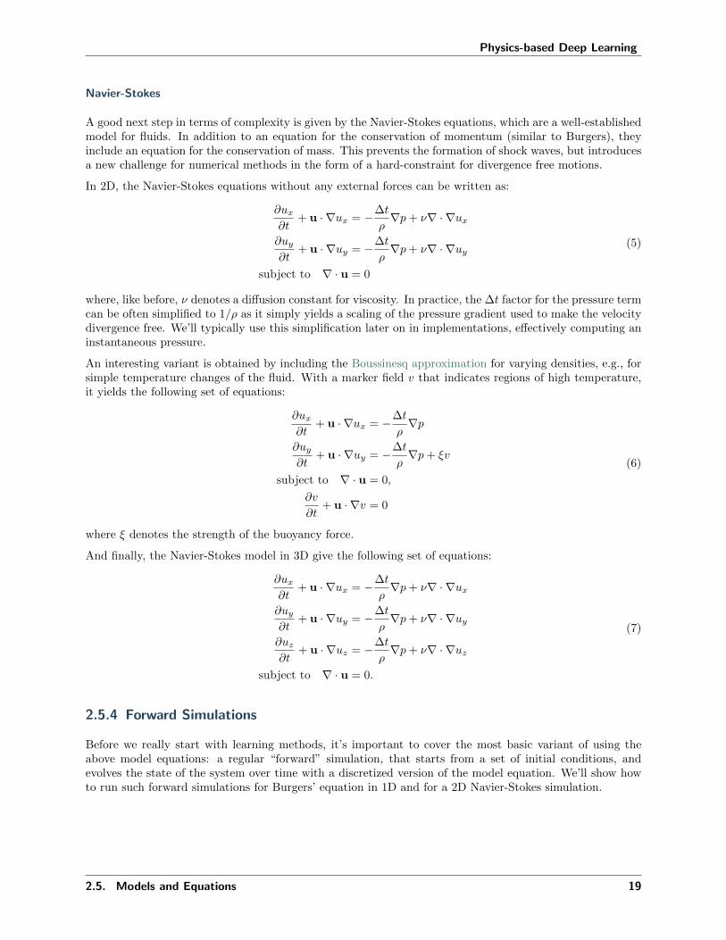
Navier-Stokes
A good next step in terms of complexity is given by the Navier-Stokes equations, which are a well-establishedmodel for fluids. In addition to an equation for the conservation of momentum (similar to Burgers), theyinclude an equation for the conservation of mass. This prevents the formation of shock waves, but introducesa new challenge for numerical methods in the form of a hard-constraint for divergence free motions.
In 2D, the Navier-Stokes equations without any external forces can be written as:
𝜕𝑢𝑥
𝜕𝑡+ u · ∇𝑢𝑥 = −∆𝑡
𝜌∇𝑝 + 𝜈∇ · ∇𝑢𝑥
𝜕𝑢𝑦
𝜕𝑡+ u · ∇𝑢𝑦 = −∆𝑡
𝜌∇𝑝 + 𝜈∇ · ∇𝑢𝑦
subject to ∇ · u = 0
(5)
where, like before, 𝜈 denotes a diffusion constant for viscosity. In practice, the ∆𝑡 factor for the pressure termcan be often simplified to 1/𝜌 as it simply yields a scaling of the pressure gradient used to make the velocitydivergence free. We’ll typically use this simplification later on in implementations, effectively computing aninstantaneous pressure.
An interesting variant is obtained by including the Boussinesq approximation for varying densities, e.g., forsimple temperature changes of the fluid. With a marker field 𝑣 that indicates regions of high temperature,it yields the following set of equations:
𝜕𝑢𝑥
𝜕𝑡+ u · ∇𝑢𝑥 = −∆𝑡
𝜌∇𝑝
𝜕𝑢𝑦
𝜕𝑡+ u · ∇𝑢𝑦 = −∆𝑡
𝜌∇𝑝 + 𝜉𝑣
subject to ∇ · u = 0,
𝜕𝑣
𝜕𝑡+ u · ∇𝑣 = 0
(6)
where 𝜉 denotes the strength of the buoyancy force.
And finally, the Navier-Stokes model in 3D give the following set of equations:
𝜕𝑢𝑥
𝜕𝑡+ u · ∇𝑢𝑥 = −∆𝑡
𝜌∇𝑝 + 𝜈∇ · ∇𝑢𝑥
𝜕𝑢𝑦
𝜕𝑡+ u · ∇𝑢𝑦 = −∆𝑡
𝜌∇𝑝 + 𝜈∇ · ∇𝑢𝑦
𝜕𝑢𝑧
𝜕𝑡+ u · ∇𝑢𝑧 = −∆𝑡
𝜌∇𝑝 + 𝜈∇ · ∇𝑢𝑧
subject to ∇ · u = 0.
(7)
2.5.4 Forward Simulations
Before we really start with learning methods, it’s important to cover the most basic variant of using theabove model equations: a regular “forward” simulation, that starts from a set of initial conditions, andevolves the state of the system over time with a discretized version of the model equation. We’ll show howto run such forward simulations for Burgers’ equation in 1D and for a 2D Navier-Stokes simulation.
2.5. Models and Equations 19
Physics-based Deep Learning
2.6 Simple Forward Simulation of Burgers Equation with phiflow
This chapter will give an introduction for how to run forward, i.e., regular simulations starting with a giveninitial state and approximating a later state numerically, and introduce the 𝜑Flow framework. 𝜑Flow providesa set of differentiable building blocks that directly interface with deep learning frameworks, and hence is avery good basis for the topics of this book. Before going for deeper and more complicated integrations, thisnotebook (and the next one), will show how regular simulations can be done with 𝜑Flow. Later on, we’llshow that these simulations can be easily coupled with neural networks.
The main repository for 𝜑Flow (in the following “phiflow”) is https://github.com/tum-pbs/PhiFlow, andadditional API documentation and examples can be found at https://tum-pbs.github.io/PhiFlow/.
For this jupyter notebook (and all following ones), you can find a “[run in colab]” link at the end of the firstparagraph (alternatively you can use the launch button at the top of the page). This will load the latestversion from the PBDL github repo in a colab notebook that you can execute on the spot: [run in colab]
2.6.1 Model
As physical model we’ll use Burgers equation. This equation is a very simple, yet non-linear and non-trivial,model equation that can lead to interesting shock formations. Hence, it’s a very good starting point forexperiments, and it’s 1D version (from equation (4)) is given by:
𝜕𝑢
𝜕𝑡+ 𝑢∇𝑢 = 𝜈∇ · ∇𝑢
2.6.2 Importing and loading phiflow
Let’s get some preliminaries out of the way: first we’ll import the phiflow library, more specifically the numpyoperators for fluid flow simulations: phi.flow (differentiable versions for a DL framework X are loaded viaphi.X.flow instead).
Note: Below, the first command with a “!” prefix will install the phiflow python package from GitHub viapip in your python environment once you uncomment it. We’ve assumed that phiflow isn’t installed, but ifyou have already done so, just comment out the first line (the same will hold for all following notebooks).
#!pip install --upgrade --quiet phiflow
!pip install --upgrade --quiet git+https://github.com/tum-pbs/PhiFlow@develop
from phi.flow import *
from phi import __version__
print("Using phiflow version: ".format(phi.__version__))
Using phiflow version: 2.0.0rc2
Next we can define and initialize the necessary constants (denoted by upper-case names): our simulationdomain will have N=128 cells as discretization points for the 1D velocity 𝑢 in a periodic domain Ω for theinterval [−1, 1]. We’ll use 32 time STEPS for a time interval of 1, giving us DT=1/32. Additionally, we’ll usea viscosity NU of 𝜈 = 0.01/𝜋.
We’ll also define an initial state given by −sin(𝜋𝑥) in the numpy array INITIAL NUMPY, which we’ll use toinitialize the velocity 𝑢 in the simulation in the next cell. This initialization will produce a nice shock in thecenter of our domain.
20 Chapter 2. Overview

Physics-based Deep Learning
Phiflow is object-oriented and centered around field data in the form of grids (internally represented by atensor object). I.e. you assemble your simulation by constructing a number of grids, and updating themover the course of time steps.
Phiflow internally works with tensors that have named dimensions. This will be especially handy later onfor 2D simulations with additional batch and channel dimensions, but for now we’ll simply convert the 1Darray into a phiflow tensor that has a single spatial dimension 'x'.
N = 128
STEPS = 32
DT = 1./STEPS
NU = 0.01/np.pi
# initialization of velocities
INITIAL_NUMPY = np.asarray( [-np.sin(np.pi * x) * 1. for x in np.linspace(-1,1,N)] ) # 1D numpy
→˓array
INITIAL = math.tensor(INITIAL_NUMPY, spatial('x') ) # convert to phiflow tensor
Next, we initialize a 1D velocity grid from the INITIAL numpy array that was converted into a tensor. Theextent of our domain Ω is specifiied via the bounds parameter [−1, 1], and the grid uses periodic boundaryconditions (extrapolation.PERIODIC). These two properties are the main difference between a tensor anda grid: the latter has boundary conditions and a physical extent.
Just to illustrate, we’ll also print some info about the velocity object: it’s a phi.math tensor with a sizeof 128. Note that the actual grid content is contained in the values of the grid. Below we’re printing fiveentries by using the numpy() function to convert the content of the phiflow tensor into a numpy array. Fortensors with more dimensions, we’d need to specify the order here, e.g., 'y,x,vector' for a 2D velocityfield. (If we’d call numpy('x,vector') below, this would convert the 1D array into one with an additionaldimension for each 1D velocity component.)
velocity = CenteredGrid(INITIAL, extrapolation.PERIODIC, x=N, bounds=Box[-1:1])
#velocity = CenteredGrid(Noise(), extrapolation.PERIODIC, x=N, bounds=Box[-1:1]) # random init
print("Velocity tensor shape: " + format( velocity.shape )) # == velocity.values.shape
print("Velocity tensor type: " + format( type(velocity.values) ))
print("Velocity tensor entries 10 to 14: " + format( velocity.values.numpy()[10:15] ))
Velocity tensor shape: (x=128)
Velocity tensor type: <class 'phi.math._tensors.CollapsedTensor'>Velocity tensor entries 10 to 14: [0.47480196 0.51774486 0.55942075 0.59972764 0.6385669 ]
2.6.3 Running the simulation
Now we’re ready to run the simulation itself. To ccompute the diffusion and advection components ofour model equation we can simply call the existing diffusion and semi lagrangian operators in phiflow:diffuse.explicit(u,...) computes an explicit diffusion step via central differences for the term 𝜈∇ · ∇𝑢of our model. Next, advect.semi lagrangian(f,u) is used for a stable first-order approximation of thetransport of an arbitrary field f by a velocity u. In our model we have 𝜕𝑢/𝜕𝑡 + 𝑢∇𝑓 , hence we use thesemi lagrangian function to transport the velocity with itself in the implementation:
velocities = [velocity]
age = 0.
for i in range(STEPS):
v1 = diffuse.explicit(velocities[-1], NU, DT)
(continues on next page)
2.6. Simple Forward Simulation of Burgers Equation with phiflow 21

Physics-based Deep Learning
(continued from previous page)
v2 = advect.semi_lagrangian(v1, v1, DT)
age += DT
velocities.append(v2)
print("New velocity content at t= : ".format( age, velocities[-1].values.numpy()[0:5] ))
New velocity content at t=1.0: [0.00274862 0.01272991 0.02360343 0.03478042 0.0460869 ]
Here we’re actually collecting all time steps in the list velocities. This is not necessary in general (andcould consume lots of memory for long-running sims), but useful here to plot the evolution of the velocitystates later on.
The print statements print a few of the velocity entries, and already show that something is happening inour simulation, but it’s difficult to get an intuition for the behavior of the PDE just from these numbers.Hence, let’s visualize the states over time to show what is happening.
2.6.4 Visualization
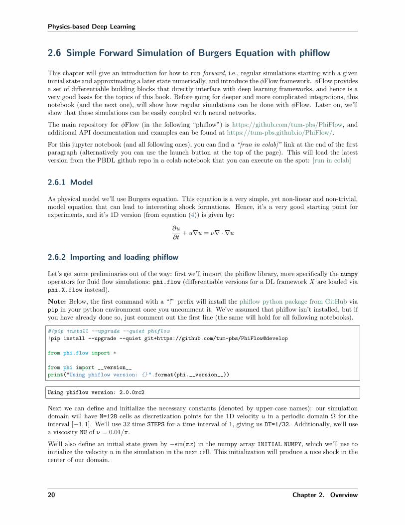
We can visualize this 1D case easily in a graph: the following code shows the initial state in blue, and thentimes 10/32, 20/32, 1 in green, cyan and purple.
# get "velocity.values" from each phiflow state with a channel dimensions, i.e. "vector"
vels = [v.values.numpy('x,vector') for v in velocities] # gives a list of 2D arrays
import pylab
fig = pylab.figure().gca()
fig.plot(np.linspace(-1,1,len(vels[ 0].flatten())), vels[ 0].flatten(), lw=2, color='blue', label=
→˓"t=0")
fig.plot(np.linspace(-1,1,len(vels[10].flatten())), vels[10].flatten(), lw=2, color='green', label=
→˓"t=0.3125")
fig.plot(np.linspace(-1,1,len(vels[20].flatten())), vels[20].flatten(), lw=2, color='cyan', label=
→˓"t=0.625")
fig.plot(np.linspace(-1,1,len(vels[32].flatten())), vels[32].flatten(), lw=2, color='purple',label=→˓"t=1")
pylab.xlabel('x'); pylab.ylabel('u'); pylab.legend()
<matplotlib.legend.Legend at 0x7f9ca2d4ef70>
22 Chapter 2. Overview
Physics-based Deep Learning
This nicely shows the shock developing in the center of our domain, which forms from the collision of thetwo initial velocity “bumps”, the positive one on left (moving right) and the negative one right of the center(moving left).
As these lines can overlap quite a bit we’ll also use a different visualization in the following chapters thatshows the evolution over the course of all time steps in a 2D image. Our 1D domain will be shown along theY-axis, and each point along X will represent one time step.
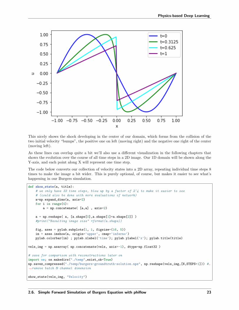
The code below converts our collection of velocity states into a 2D array, repeating individual time steps 8times to make the image a bit wider. This is purely optional, of course, but makes it easier to see what’shappening in our Burgers simulation.
def show_state(a, title):
# we only have 33 time steps, blow up by a factor of 2^4 to make it easier to see
# (could also be done with more evaluations of network)
a=np.expand_dims(a, axis=2)
for i in range(4):
a = np.concatenate( [a,a] , axis=2)
a = np.reshape( a, [a.shape[0],a.shape[1]*a.shape[2]] )
#print("Resulting image size" +format(a.shape))
fig, axes = pylab.subplots(1, 1, figsize=(16, 5))
im = axes.imshow(a, origin='upper', cmap='inferno')pylab.colorbar(im) ; pylab.xlabel('time'); pylab.ylabel('x'); pylab.title(title)
vels_img = np.asarray( np.concatenate(vels, axis=-1), dtype=np.float32 )
# save for comparison with reconstructions later on
import os; os.makedirs("./temp",exist_ok=True)
np.savez_compressed("./temp/burgers-groundtruth-solution.npz", np.reshape(vels_img,[N,STEPS+1])) #
→˓remove batch & channel dimension
show_state(vels_img, "Velocity")
2.6. Simple Forward Simulation of Burgers Equation with phiflow 23
Physics-based Deep Learning
This concludes a first simulation in phiflow. It’s not overly complex, but because of that it’s a good startingpoint for evaluating and comparing different physics-based deep learning approaches in the next chapter.But before that, we’ll target a more complex simulation type in the next section.
2.6.5 Next steps
Some things to try based on this simulation setup:
• Feel free to experiment - the setup above is very simple, you can change the simulation parameters,or the initialization. E.g., you can use a noise field via Noise() to get more chaotic results (cf. thecomment in the velocity cell above).
• A bit more complicated: extend the simulation to 2D (or higher). This will require changes throughout,but all operators above support higher dimensions. Before trying this, you probably will want to checkout the next example, which covers a 2D Navier-Stokes case.
2.7 Navier-Stokes Forward Simulation
Now let’s target a somewhat more complex example: a fluid simulation based on the Navier-Stokes equations.This is still very simple with 𝜑Flow (phiflow), as differentiable operators for all steps exist there. The Navier-Stokes equations (in their incompressible form) introduce an additional pressure field 𝑝, and a constraint forconservation of mass, as introduced in equation (6). We’re also moving a marker field, denoted by 𝑑 here,with the flow. It indicates regions of higher temperature, and exerts a force via a buouyancy factor 𝜉:
𝜕u
𝜕𝑡+ u · ∇u = −1
𝜌∇𝑝 + 𝜈∇ · ∇u + (0, 1)𝑇 𝜉𝑑 s.t. ∇ · u = 0,
𝜕𝑑
𝜕𝑡+ u · ∇𝑑 = 0
Here, we’re aiming for an incompressible flow (i.e., 𝜌 = const), and use a simple buoyancy model (the Boussi-nesq approximation) via the term (0, 1)𝑇 𝜉𝑑. This models changes in density without explicitly calculating 𝜌,and we assume a gravity force that acts along the y direction via the vector (0, 1)𝑇 . We’ll solve this PDE ona closed domain with Dirichlet boundary conditions u = 0 for the velocity, and Neumann boundaries 𝜕𝑝
𝜕𝑥 = 0for pressure, on a domain Ω with a physical size of 100 × 80 units. [run in colab]
24 Chapter 2. Overview

Physics-based Deep Learning
2.7.1 Implementation
As in the previous section, the first command with a “!” prefix installs the phiflow python package fromGitHub via pip in your python environment. (Skip or modify this command if necessary.)
#!pip install --upgrade --quiet phiflow
!pip install --upgrade --quiet git+https://github.com/tum-pbs/PhiFlow@develop
from phi.flow import * # The Dash GUI is not supported on Google colab, ignore the warning
import pylab
2.7.2 Setting up the simulation
The following code sets up a few constants, which are denoted by upper case names. We’ll use 40 × 32 cellsto discretize our domain, introduce a slight viscosity via 𝜈, and define the time step to be ∆𝑡 = 1.5.
We’re creating a first CenteredGrid here, which is initialized by a Sphere geometry object. This willrepresent the inflow region INFLOW where hot smoke is generated.
DT = 1.5
NU = 0.01
INFLOW = CenteredGrid(Sphere(center=(30,15), radius=10), extrapolation.BOUNDARY, x=32, y=40,
→˓bounds=Box[0:80, 0:100]) * 0.2
The inflow will be used to inject smoke into a second centered grid smoke that represents the marker field𝑑 from above. Note that we’ve defined a Box of size 100𝑥80 above. This is the physical scale in terms ofspatial units in our simulation, i.e., a velocity of magnitude 1 will move the smoke density by 1 unit per 1time unit, which may be larger or smaller than a cell in the discretized grid, depending on the settings forx,y. You could parametrize your simulation grid to directly resemble real-world units, or keep appropriateconversion factors in mind.
The inflow sphere above is already using the “world” coordinates: it is located at 𝑥 = 30 along the first axis,and 𝑦 = 15 (within the 100𝑥80 domain box).
Next, we create grids for the quantities we want to simulate. For this example, we require a velocity fieldand a smoke density field.
smoke = CenteredGrid(0, extrapolation.BOUNDARY, x=32, y=40, bounds=Box[0:80, 0:100]) # sampled at
→˓cell centers
velocity = StaggeredGrid(0, extrapolation.ZERO, x=32, y=40, bounds=Box[0:80, 0:100]) # sampled in
→˓staggered form at face centers
We sample the smoke field at the cell centers and the velocity in staggered form. The staggered gridinternally contains 2 centered grids with different dimensions, and can be converted into centered grids (orsimply numpy arrays) via the unstack function, as explained in the link above.
Next we define the update step of the simulation, which calls the necessary functions to advance the stateof our fluid system by dt. The next cell computes one such step, and plots the marker density after onesimulation frame.
def step(velocity, smoke, pressure, dt=1.0, buoyancy_factor=1.0):
smoke = advect.semi_lagrangian(smoke, velocity, dt) + INFLOW
buoyancy_force = smoke * (0, buoyancy_factor) >> velocity # resamples smoke to velocity
→˓sample points
velocity = advect.semi_lagrangian(velocity, velocity, dt) + dt * buoyancy_force
(continues on next page)
2.7. Navier-Stokes Forward Simulation 25

Physics-based Deep Learning
(continued from previous page)
velocity = diffuse.explicit(velocity, NU, dt)
velocity, pressure = fluid.make_incompressible(velocity)
return velocity, smoke, pressure
velocity, smoke, pressure = step(velocity, smoke, None, dt=DT)
print("Max. velocity and mean marker density: " + format( [ math.max(velocity.values) , math.
→˓mean(smoke.values) ] ))
pylab.imshow(np.asarray(smoke.values.numpy('y,x')), origin='lower', cmap='magma')
Max. velocity and mean marker density: [0.15530995, 0.008125]
<matplotlib.image.AxesImage at 0x7fa2f8d16eb0>
A lot has happened in this step() call: we’ve advected the smoke field, added an upwards force via aBoussinesq model, advected the velocity field, and finally made it divergence free via a pressure solve.
The Boussinesq model uses a multiplication by a tuple (0, buoyancy factor) to turn the smoke fieldinto a staggered, 2 component force field, sampled at the locations of the velocity components via the>> operator. This operator makes sure the individual force components are correctly interpolated for thevelocity components of the staggered velocity. >> could be rewritten via the sampling function at() as(smoke*(0,buoyancy factor)).at(velocity). However, >> also directly ensure the boundary conditionsof the original grid are kept. Hence, it internally also does StaggeredGrid(..., extrapolation.ZERO,..
.) for the force grid. Long story short: the >> operator does the same thing, and typically produces shorterand more readable code.
The pressure projection step in make incompressible is typically the computationally most expensive stepin the sequence above. It solves a Poisson equation for the boundary conditions of the domain, and updatesthe velocity field with the gradient of the computed pressure.
Just for testing, we’ve also printed the mean value of the velocities, and the max density after the update.As you can see in the resulting image, we have a first round region of smoke, with a slight upwards motion
26 Chapter 2. Overview

Physics-based Deep Learning
(which does not show here yet).
2.7.3 Datatypes and dimensions
The variables we created for the fields of the simulation here are instances of the class Grid. Like tensors,grids also have the shape attribute which lists all batch, spatial and channel dimensions. Shapes in phiflowstore not only the sizes of the dimensions but also their names and types.
print(f"Smoke: smoke.shape ")
print(f"Velocity: velocity.shape ")
print(f"Inflow: INFLOW.shape , spatial only: INFLOW.shape.spatial ")
Smoke: (x=32, y=40)
Velocity: (x=32, y=40, vector=2)
Inflow: (x=32, y=40), spatial only: (x=32, y=40)
Note that the phiflow output here indicates the type of a dimension, e.g., 𝑆 for a spatial, and 𝑉 for a vectordimension. Later on for learning, we’ll also introduce batch dimensions.
The actual content of a shape object can be obtained via .sizes, or alternatively we can query the size ofa specific dimension dim via .get size('dim'). Here are two examples:
print(f"Shape content: velocity.shape.sizes ")
print(f"Vector dimension: velocity.shape.get_size('vector') ")
Shape content: (32, 40, 2)
Vector dimension: 2
The grid values can be accessed using the values property. This is an important difference to a phiflowtensor object, which does not have values, as illustrated in the code example below.
print("Statistics of the different simulation grids:")
print(smoke.values)
print(velocity.values)
# in contrast to a simple tensor:
test_tensor = math.tensor(numpy.zeros([2, 5, 3]), spatial('x,y'), channel('vector'))print("Reordered test tensor shape: " + format(test_tensor.numpy('vector,y,x').shape) )
#print(test_tensor.values.numpy('y,x')) # error! tensors don't return their content via ".values"
Statistics of the different simulation grids:
(x=32, y=40) float32 0.0 < ... < 0.20000000298023224
(x=(31, 32), y=(40, 39), vector=2) float32 -0.12352858483791351 < ... < 0.15530994534492493
Reordered test tensor shape: (3, 5, 2)
Grids have many more properties which are documented here. Also note that the staggered grid has anon-uniform shape because the number of faces is not equal to the number of cells (in this example the xcomponent has 31 × 40 cells, while y has 32 × 39). The INFLOW grid naturally has the same dimensions asthe smoke grid.
2.7. Navier-Stokes Forward Simulation 27
Physics-based Deep Learning
2.7.4 Time evolution
With this setup, we can easily advance the simulation forward in time a bit more by repeatedly calling thestep function.
for time_step in range(10):
velocity, smoke, pressure = step(velocity, smoke, pressure, dt=DT)
print('Computed frame , max velocity '.format(time_step , np.asarray(math.max(velocity.
→˓values)) ))
Computed frame 0, max velocity 0.4609803557395935
Computed frame 1, max velocity 0.8926814794540405
Computed frame 2, max velocity 1.4052708148956299
Computed frame 3, max velocity 2.036500930786133
Computed frame 4, max velocity 2.921010971069336
Computed frame 5, max velocity 3.828195810317993
Computed frame 6, max velocity 4.516851425170898
Computed frame 7, max velocity 4.861286640167236
Computed frame 8, max velocity 5.125314235687256
Computed frame 9, max velocity 5.476282119750977
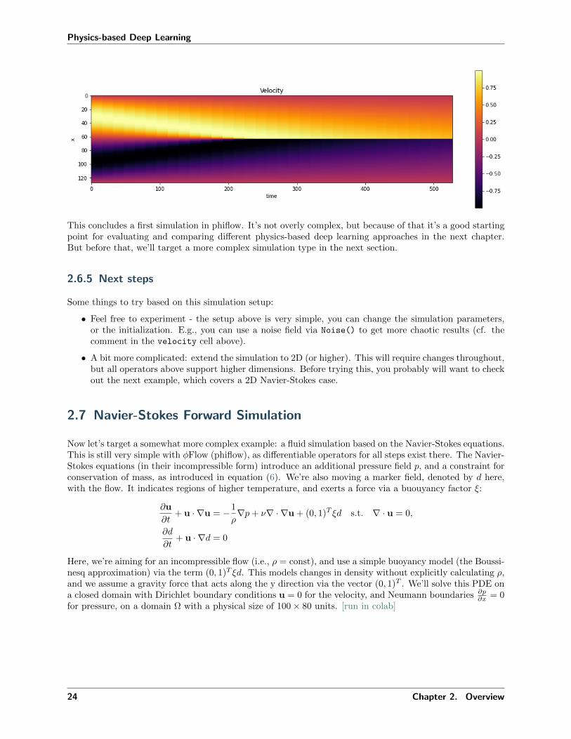
Now the hot plume is starting to rise:
pylab.imshow(smoke.values.numpy('y,x'), origin='lower', cmap='magma')
<matplotlib.image.AxesImage at 0x7fa2f902cf40>
Let’s compute and show a few more steps of the simulation. Because of the inflow being located off-center tothe left (with x position 30), the plume will curve towards the right when it hits the top wall of the domain.
steps = [[ smoke.values, velocity.values.vector[0], velocity.values.vector[1] ]]
for time_step in range(20):
if time_step<3 or time_step%10==0:
(continues on next page)
28 Chapter 2. Overview

Physics-based Deep Learning
(continued from previous page)
print('Computing time step %d ' % time_step)
velocity, smoke, pressure = step(velocity, smoke, pressure, dt=DT)
if time_step%5==0:
steps.append( [smoke.values, velocity.values.vector[0], velocity.values.vector[1]] )
fig, axes = pylab.subplots(1, len(steps), figsize=(16, 5))
for i in range(len(steps)):
axes[i].imshow(steps[i][0].numpy('y,x'), origin='lower', cmap='magma')axes[i].set_title(f"d at t= i*5 ")
Computing time step 0
Computing time step 1
Computing time step 2
Computing time step 10
We can also take a look at the velocities. The steps list above already stores vector[0] and vector[1]
components of the velocities as numpy arrays, which we can show next.
fig, axes = pylab.subplots(1, len(steps), figsize=(16, 5))
for i in range(len(steps)):
axes[i].imshow(steps[i][1].numpy('y,x'), origin='lower', cmap='magma')axes[i].set_title(f"u_x at t= i*5 ")
fig, axes = pylab.subplots(1, len(steps), figsize=(16, 5))
for i in range(len(steps)):
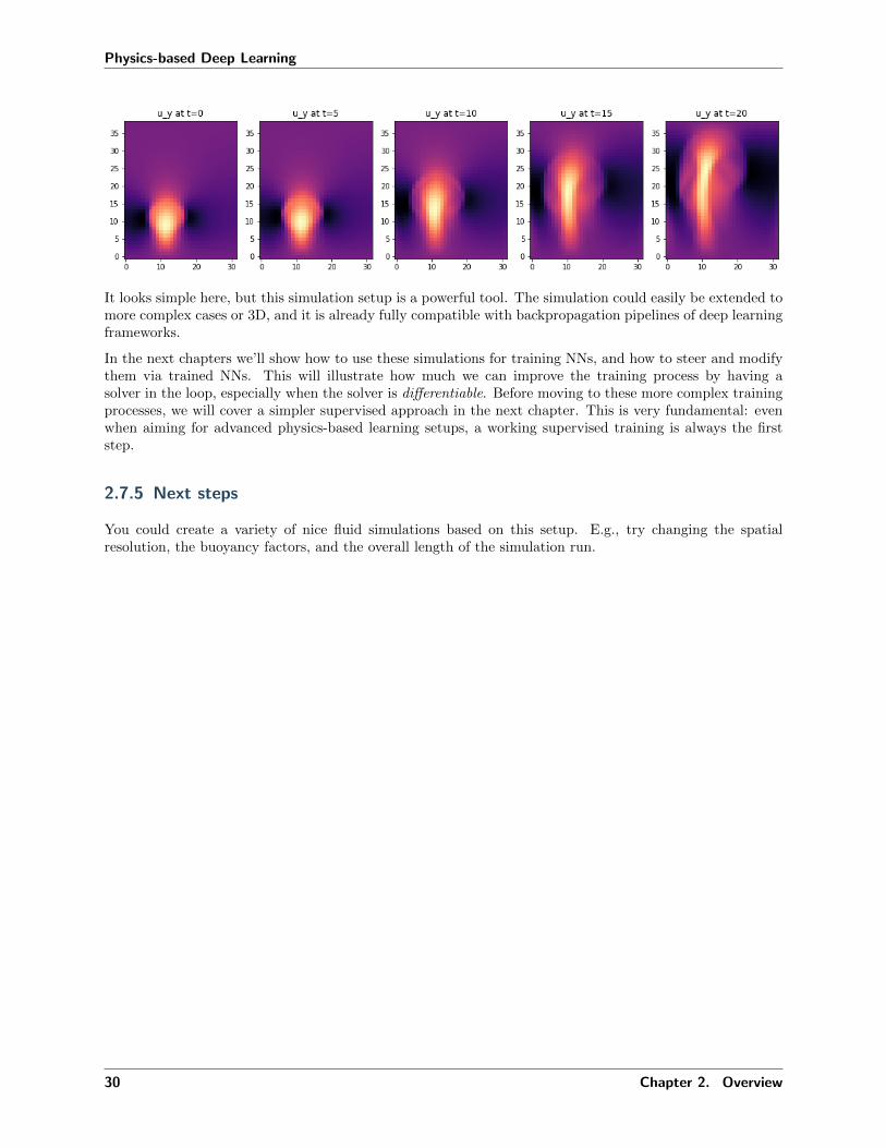
axes[i].imshow(steps[i][2].numpy('y,x'), origin='lower', cmap='magma')axes[i].set_title(f"u_y at t= i*5 ")
2.7. Navier-Stokes Forward Simulation 29
Physics-based Deep Learning
It looks simple here, but this simulation setup is a powerful tool. The simulation could easily be extended tomore complex cases or 3D, and it is already fully compatible with backpropagation pipelines of deep learningframeworks.
In the next chapters we’ll show how to use these simulations for training NNs, and how to steer and modifythem via trained NNs. This will illustrate how much we can improve the training process by having asolver in the loop, especially when the solver is differentiable. Before moving to these more complex trainingprocesses, we will cover a simpler supervised approach in the next chapter. This is very fundamental: evenwhen aiming for advanced physics-based learning setups, a working supervised training is always the firststep.
2.7.5 Next steps
You could create a variety of nice fluid simulations based on this setup. E.g., try changing the spatialresolution, the buoyancy factors, and the overall length of the simulation run.
30 Chapter 2. Overview

CHAPTER
THREE
SUPERVISED TRAINING
Supervised here essentially means: “doing things the old fashioned way”. Old fashioned in the context ofdeep learning (DL), of course, so it’s still fairly new. Also, “old fashioned” doesn’t always mean bad - it’sjust that later on we’ll discuss ways to train networks that clearly outperform approaches using supervisedtraining.
Nonetheless, “supervised training” is a starting point for all projects one would encounter in the context ofDL, and hence it is worth studying. Also, while it typically yields inferior results to approaches that moretightly couple with physics, it can be the only choice in certain application scenarios where no good modelequations exist.
3.1 Problem setting
For supervised training, we’re faced with an unknown function 𝑓*(𝑥) = 𝑦*, collect lots of pairs of data[𝑥0, 𝑦
*0 ], ...[𝑥𝑛, 𝑦
*𝑛] (the training data set) and directly train an NN to represent an approximation of 𝑓*
denoted as 𝑓 .
The 𝑓 we can obtain in this way is typically not exact, but instead we obtain it via a minimization problem:by adjusting the weights 𝜃 of our NN representation of 𝑓 such that
arg min𝜃
∑𝑖
(𝑓(𝑥𝑖; 𝜃) − 𝑦*𝑖 )2. (1)
This will give us 𝜃 such that 𝑓(𝑥; 𝜃) = 𝑦 ≈ 𝑦* as accurately as possible given our choice of 𝑓 and thehyperparameters for training. Note that above we’ve assumed the simplest case of an 𝐿2 loss. A moregeneral version would use an error metric 𝑒(𝑥, 𝑦) to be minimized via arg min𝜃
∑𝑖 𝑒(𝑓(𝑥𝑖; 𝜃), 𝑦*𝑖 )). The
choice of a suitable metric is a topic we will get back to later on.
Irrespective of our choice of metric, this formulation gives the actual “learning” process for a supervisedapproach.
The training data typically needs to be of substantial size, and hence it is attractive to use numericalsimulations solving a physical model 𝒫 to produce a large number of reliable input-output pairs for training.This means that the training process uses a set of model equations, and approximates them numerically, inorder to train the NN representation 𝑓 . This has quite a few advantages, e.g., we don’t have measurementnoise of real-world devices and we don’t need manual labour to annotate a large number of samples to gettraining data.
On the other hand, this approach inherits the common challenges of replacing experiments with simulations:first, we need to ensure the chosen model has enough power to predict the behavior of real-world phenomenathat we’re interested in. In addition, the numerical approximations have numerical errors which need to bekept small enough for a chosen application. As these topics are studied in depth for classical simulations,and the existing knowledge can likewise be leveraged to set up DL training tasks.
31

Physics-based Deep Learning
Figure1: A visual overview of supervised training. Quite simple overall, but it’s good to keep this in mindin comparison to the more complex variants we’ll encounter later on.
3.2 Surrogate models
One of the central advantages of the supervised approach above is that we obtain a surrogate model, i.e.,a new function that mimics the behavior of the original 𝒫. The numerical approximations of PDE modelsfor real world phenomena are often very expensive to compute. A trained NN on the other hand incurs aconstant cost per evaluation, and is typically trivial to evaluate on specialized hardware such as GPUs orNN units.
Despite this, it’s important to be careful: NNs can quickly generate huge numbers of in between results.Consider a CNN layer with 128 features. If we apply it to an input of 1282, i.e. ca. 16k cells, we get 1283
intermediate values. That’s more than 2 million. All these values at least need to be momentarily stored inmemory, and processed by the next layer.
Nonetheless, replacing complex and expensive solvers with fast, learned approximations is a very attractiveand interesting direction.
3.3 Show me some code!
Let’s finally look at a code example that trains a neural network: we’ll replace a full solver for turbulentflows around airfoils with a surrogate model from [TWPH20].
3.4 Supervised training for RANS flows around airfoils
3.4.1 Overview
For this example of supervised training we have a turbulent airflow around wing profiles, and we’d like toknow the average motion and pressure distribution around this airfoil for different Reynolds numbers andangles of attack. Thus, given an airfoil shape, Reynolds numbers, and angle of attack, we’d like to obtain avelocity field and a pressure field around the airfoil.
This is classically approximated with Reynolds-Averaged Navier Stokes (RANS) models, and this setting isstill one of the most widely used applications of Navier-Stokes solver in industry. However, instead of relyingon traditional numerical methods to solve the RANS equations, we now aim for training a surrogate model
32 Chapter 3. Supervised Training

Physics-based Deep Learning
via a neural network that completely bypasses the numerical solver, and produces the solution in terms ofvelocity and pressure. [run in colab]
3.4.2 Formulation
With the supervised formulation from Supervised Training , our learning task is pretty straight-forward, andcan be written as
arg min𝜃
∑𝑖
(𝑓(𝑥𝑖; 𝜃) − 𝑦*𝑖 )2,
where 𝑥 and 𝑦* each consist of a set of physical fields, and the index 𝑖 evaluates the difference across alldiscretization points in our data sets.
The goal is to infer velocity u = 𝑢𝑥, 𝑢𝑦 and a pressure field 𝑝 in a computational domain Ω around the airfoilin the center of Ω. 𝑢𝑥, 𝑢𝑦 and 𝑝 each have a dimension of 1282. As inputs we have the Reynolds numberRe ∈ R, the angle of attack 𝛼 ∈ R, and the airfoil shape s encoded as a rasterized grid with 1282. Bothconstant, scalar inputs Re and 𝛼 are likewise extended to a size of 1282. Thus, put together, both inputand output have the same dimensions: 𝑥, 𝑦* ∈ R3×128×128. This is exactly what we’ll specify as input andoutput dimensions for the NN below.
A point to keep in mind here is that our quantities of interest in 𝑦* contain three different physical fields.While the two velocity components are quite similar in spirit, the pressure field typically has a differentbehavior with an approximately squared scaling with respect to the velocity (cf. Bernoulli). This impliesthat we need to be careful with simple summations (as in the minimization problem above), and that weshould take care to normalize the data.
3.4.3 Code coming up...
Let’s get started with the implementation. Note that we’ll skip the data generation process here. The codebelow is adapted from [TWPH20] and this codebase, which you can check out for details. Here, we’ll simplydownload a small set of training data generated with a Spalart-Almaras RANS simulation in OpenFOAM.
import numpy as np
import os.path, random
import torch
from torch.utils.data import Dataset
print("Torch version ".format(torch.__version__))
# get training data
dir = "./"
if True:
# download
if not os.path.isfile('data-airfoils.npz'):import requests
print("Downloading training data (300MB), this can take a few minutes the first time...")
with open("data-airfoils.npz", 'wb') as datafile:
resp = requests.get('https://dataserv.ub.tum.de/s/m1615239/download?path=%2F &files=dfp-→˓data-400.npz', verify=False)
datafile.write(resp.content)
else:
# alternative: load from google drive (upload there beforehand):
from google.colab import drive
drive.mount('/content/gdrive')dir = "./gdrive/My Drive/"
(continues on next page)
3.4. Supervised training for RANS flows around airfoils 33

Physics-based Deep Learning
(continued from previous page)
npfile=np.load(dir+'data-airfoils.npz')
print("Loaded data, training, validation samples".format(len(npfile["inputs"]),len(npfile[
→˓"vinputs"])))
print("Size of the inputs array: "+format(npfile["inputs"].shape))
Torch version 1.8.1+cu101
Downloading training data (300MB), this can take a few minutes the first time...
Loaded data, 320 training, 80 validation samples
Size of the inputs array: (320, 3, 128, 128)
If you run this notebook in colab, the else statement above (which is deactivated by default) might beinteresting for you: instead of downloading the training data anew every time, you can manually downloadit once and store it in your google drive. We assume it’s stored in the root directory as data-airfoils.npz.Afterwards, you can use the code above to load the file from your google drive, which is typically muchfaster. This is highly recommended if you want to experiment more extensively via colab.
3.4.4 RANS training data
Now we have some training data. In general it’s very important to understand the data we’re working withas much as possible (for any ML task the garbage-in-gargabe-out principle definitely holds). We should atleast understand the data in terms of dimensions and rough statistics, but ideally also in terms of content.Otherwise we’ll have a very hard time interpreting the results of a training run. And despite all the DLmagic: if you can’t make out any patterns in your data, NNs surely won’t find any useful ones.
Hence, let’s look at one of the training samples... The following is just some helper code to show images sideby side.
import pylab
# helper to show three target channels: normalized, with colormap, side by side
def showSbs(a1,a2, stats=False, bottom="NN Output", top="Reference", title=None):
c=[]
for i in range(3):
b = np.flipud( np.concatenate((a2[i],a1[i]),axis=1).transpose())
min, mean, max = np.min(b), np.mean(b), np.max(b);
if stats: print("Stats %d : "%i + format([min,mean,max]))
b -= min; b /= (max-min)
c.append(b)
fig, axes = pylab.subplots(1, 1, figsize=(16, 5))
axes.set_xticks([]); axes.set_yticks([]);
im = axes.imshow(np.concatenate(c,axis=1), origin='upper', cmap='magma')
pylab.colorbar(im); pylab.xlabel('p, ux, uy'); pylab.ylabel('%s %s '%(bottom,top))if title is not None: pylab.title(title)
NUM=72
showSbs(npfile["inputs"][NUM],npfile["targets"][NUM], stats=False, bottom="Target Output", top=
→˓"Inputs", title="3 inputs are shown at the top (mask, in-ux, in-uy), with the 3 output channels
→˓(p,ux,uy) at the bottom")
34 Chapter 3. Supervised Training

Physics-based Deep Learning
Next, let’s define a small helper class DfpDataset to organize inputs and targets. We’ll transfer the corre-sponding data to the pytorch DataLoader class.
We also set up some globals to control training parameters, maybe most importantly: the learning rate LR,i.e. 𝜂 from the previous setions. When your training run doesn’t converge this is the first parameter toexperiment with.
Here, we’ll keep it relatively small throughout. (Using learning rate decay would be better, i.e. potentiallygive an improed convergence, but is omitted here for clarity.)
# some global training constants
# number of training epochs
EPOCHS = 100
# batch size
BATCH_SIZE = 10
# learning rate
LR = 0.00002
class DfpDataset():
def __init__(self, inputs,targets):
self.inputs = inputs
self.targets = targets
def __len__(self):
return len(self.inputs)
def __getitem__(self, idx):
return self.inputs[idx], self.targets[idx]
tdata = DfpDataset(npfile["inputs"],npfile["targets"])
vdata = DfpDataset(npfile["vinputs"],npfile["vtargets"])
trainLoader = torch.utils.data.DataLoader(tdata, batch_size=BATCH_SIZE, shuffle=True , drop_
→˓last=True)
valiLoader = torch.utils.data.DataLoader(vdata, batch_size=BATCH_SIZE, shuffle=False, drop_
→˓last=True)(continues on next page)
3.4. Supervised training for RANS flows around airfoils 35

Physics-based Deep Learning
(continued from previous page)
print("Training & validation batches: , ".format(len(trainLoader),len(valiLoader) ))
Training & validation batches: 32 , 8
3.4.5 Network setup
Now we can set up the architecture of our neural network, we’ll use a fully convolutional U-net. This isa widely used architecture that uses a stack of convolutions across different spatial resolutions. The maindeviation from a regular conv-net is to introduce skip connection from the encoder to the decoder part. Thisensures that no information is lost during feature extraction. (Note that this only works if the network is tobe used as a whole. It doesn’t work in situations where we’d, e.g., want to use the decoder as a standalonecomponent.)
Here’s a overview of the architecure:
First, we’ll define a helper to set up a convolutional block in the network, blockUNet. Note, we don’t useany pooling! Instead we use strides and transpose convolutions (these need to be symmetric for the decoderpart, i.e. have an uneven kernel size), following best practices. The full pytroch neural network is managedvia the DfpNet class.
import os, sys, random
import numpy as np
import torch
import torch.nn as nn
import torch.optim as optim
import torch.autograd
import torch.utils.data
def blockUNet(in_c, out_c, name, transposed=False, bn=True, relu=True, size=4, pad=1, dropout=0.):
block = nn.Sequential()
if relu:
block.add_module('%s _relu' % name, nn.ReLU(inplace=True))
else:
block.add_module('%s _leakyrelu' % name, nn.LeakyReLU(0.2, inplace=True))
if not transposed:
block.add_module('%s _conv' % name, nn.Conv2d(in_c, out_c, kernel_size=size, stride=2,
→˓padding=pad, bias=True))
else:
block.add_module('%s _upsam' % name, nn.Upsample(scale_factor=2, mode='bilinear'))# reduce kernel size by one for the upsampling (ie decoder part)
(continues on next page)
36 Chapter 3. Supervised Training

Physics-based Deep Learning
(continued from previous page)
block.add_module('%s _tconv' % name, nn.Conv2d(in_c, out_c, kernel_size=(size-1), stride=1,
→˓padding=pad, bias=True))
if bn:
block.add_module('%s _bn' % name, nn.BatchNorm2d(out_c))
if dropout>0.:
block.add_module('%s _dropout' % name, nn.Dropout2d( dropout, inplace=True))
return block
class DfpNet(nn.Module):
def __init__(self, channelExponent=6, dropout=0.):
super(DfpNet, self).__init__()
channels = int(2 ** channelExponent + 0.5)
self.layer1 = nn.Sequential()
self.layer1.add_module('layer1', nn.Conv2d(3, channels, 4, 2, 1, bias=True))
self.layer2 = blockUNet(channels , channels*2, 'enc_layer2', transposed=False, bn=True,
→˓relu=False, dropout=dropout )
self.layer3 = blockUNet(channels*2, channels*2, 'enc_layer3', transposed=False, bn=True,
→˓relu=False, dropout=dropout )
self.layer4 = blockUNet(channels*2, channels*4, 'enc_layer4', transposed=False, bn=True,
→˓relu=False, dropout=dropout )
self.layer5 = blockUNet(channels*4, channels*8, 'enc_layer5', transposed=False, bn=True,
→˓relu=False, dropout=dropout )
self.layer6 = blockUNet(channels*8, channels*8, 'enc_layer6', transposed=False, bn=True,
→˓relu=False, dropout=dropout , size=2,pad=0)
self.layer7 = blockUNet(channels*8, channels*8, 'enc_layer7', transposed=False, bn=True,
→˓relu=False, dropout=dropout , size=2,pad=0)
# note, kernel size is internally reduced by one for the decoder part
self.dlayer7 = blockUNet(channels*8, channels*8, 'dec_layer7', transposed=True, bn=True,
→˓relu=True, dropout=dropout , size=2,pad=0)
self.dlayer6 = blockUNet(channels*16,channels*8, 'dec_layer6', transposed=True, bn=True,
→˓relu=True, dropout=dropout , size=2,pad=0)
self.dlayer5 = blockUNet(channels*16,channels*4, 'dec_layer5', transposed=True, bn=True,
→˓relu=True, dropout=dropout )
self.dlayer4 = blockUNet(channels*8, channels*2, 'dec_layer4', transposed=True, bn=True,
→˓relu=True, dropout=dropout )
self.dlayer3 = blockUNet(channels*4, channels*2, 'dec_layer3', transposed=True, bn=True,
→˓relu=True, dropout=dropout )
self.dlayer2 = blockUNet(channels*4, channels , 'dec_layer2', transposed=True, bn=True,
→˓relu=True, dropout=dropout )
self.dlayer1 = nn.Sequential()
self.dlayer1.add_module('dec_layer1_relu', nn.ReLU(inplace=True))
self.dlayer1.add_module('dec_layer1_tconv', nn.ConvTranspose2d(channels*2, 3, 4, 2, 1,
→˓bias=True))
def forward(self, x):
# note, this Unet stack could be allocated with a loop, of course...
out1 = self.layer1(x)
out2 = self.layer2(out1)
out3 = self.layer3(out2)
out4 = self.layer4(out3)
(continues on next page)
3.4. Supervised training for RANS flows around airfoils 37

Physics-based Deep Learning
(continued from previous page)
out5 = self.layer5(out4)
out6 = self.layer6(out5)
out7 = self.layer7(out6)
# ... bottleneck ...
dout6 = self.dlayer7(out7)
dout6_out6 = torch.cat([dout6, out6], 1)
dout6 = self.dlayer6(dout6_out6)
dout6_out5 = torch.cat([dout6, out5], 1)
dout5 = self.dlayer5(dout6_out5)
dout5_out4 = torch.cat([dout5, out4], 1)
dout4 = self.dlayer4(dout5_out4)
dout4_out3 = torch.cat([dout4, out3], 1)
dout3 = self.dlayer3(dout4_out3)
dout3_out2 = torch.cat([dout3, out2], 1)
dout2 = self.dlayer2(dout3_out2)
dout2_out1 = torch.cat([dout2, out1], 1)
dout1 = self.dlayer1(dout2_out1)
return dout1
def weights_init(m):
classname = m.__class__.__name__
if classname.find('Conv') != -1:
m.weight.data.normal_(0.0, 0.02)
elif classname.find('BatchNorm') != -1:
m.weight.data.normal_(1.0, 0.02)
m.bias.data.fill_(0)
Next, we can initialize an instance of the DfpNet.
Below, the EXPO parameter here controls the exponent for the feature maps of our Unet: this directly scalesthe network size (3 gives a network with ca. 150k parameters). This is relatively small for a generative NNwith 3 × 1282 = ca. 49𝑘 outputs, but yields fast training times and prevents overfitting given the relativelysmall data set we’re using here. Hence it’s a good starting point.
# channel exponent to control network size
EXPO = 3
# setup network
net = DfpNet(channelExponent=EXPO)
#print(net) # to double check the details...
nn_parameters = filter(lambda p: p.requires_grad, net.parameters())
params = sum([np.prod(p.size()) for p in nn_parameters])
# crucial parameter to keep in view: how many parameters do we have?
print("Trainable params: -> crucial! always keep in view... ".format(params))
net.apply(weights_init)
criterionL1 = nn.L1Loss()
optimizerG = optim.Adam(net.parameters(), lr=LR, betas=(0.5, 0.999), weight_decay=0.0)
targets = torch.autograd.Variable(torch.FloatTensor(BATCH_SIZE, 3, 128, 128))
inputs = torch.autograd.Variable(torch.FloatTensor(BATCH_SIZE, 3, 128, 128))
Trainable params: 147555 -> crucial! always keep in view...
38 Chapter 3. Supervised Training

Physics-based Deep Learning
With an exponent of 3, this network has 147555 trainable parameters. As the subtle hint in the printstatement indicates, this is a crucial number to always have in view when training NNs. It’s easy to changesettings, and get a network that has millions of parameters, and as a result probably all kinds of convergenceand overfitting problems. The number of parameters definitely has to be matched with the amount oftraining data, and should also scale with the depth of the network. How these three relate to each otherexactly is problem dependent, though.
3.4.6 Training
Finally, we can train the NN. This step can take a while, as the training runs over all 320 samples 100 times,and continually evaluates the validation samples to keep track of how well the current state of the NN isdoing.
history_L1 = []
history_L1val = []
if os.path.isfile("network"):
print("Found existing network, loading & skipping training")
net.load_state_dict(torch.load("network")) # optionally, load existing network
else:
print("Training from scratch")
for epoch in range(EPOCHS):
net.train()
L1_accum = 0.0
for i, traindata in enumerate(trainLoader, 0):
inputs_curr, targets_curr = traindata
inputs.data.copy_(inputs_curr.float())
targets.data.copy_(targets_curr.float())
net.zero_grad()
gen_out = net(inputs)
lossL1 = criterionL1(gen_out, targets)
lossL1.backward()
optimizerG.step()
L1_accum += lossL1.item()
# validation
net.eval()
L1val_accum = 0.0
for i, validata in enumerate(valiLoader, 0):
inputs_curr, targets_curr = validata
inputs.data.copy_(inputs_curr.float())
targets.data.copy_(targets_curr.float())
outputs = net(inputs)
outputs_curr = outputs.data.cpu().numpy()
lossL1val = criterionL1(outputs, targets)
L1val_accum += lossL1val.item()
# data for graph plotting
history_L1.append( L1_accum / len(trainLoader) )
history_L1val.append( L1val_accum / len(valiLoader) )
(continues on next page)
3.4. Supervised training for RANS flows around airfoils 39
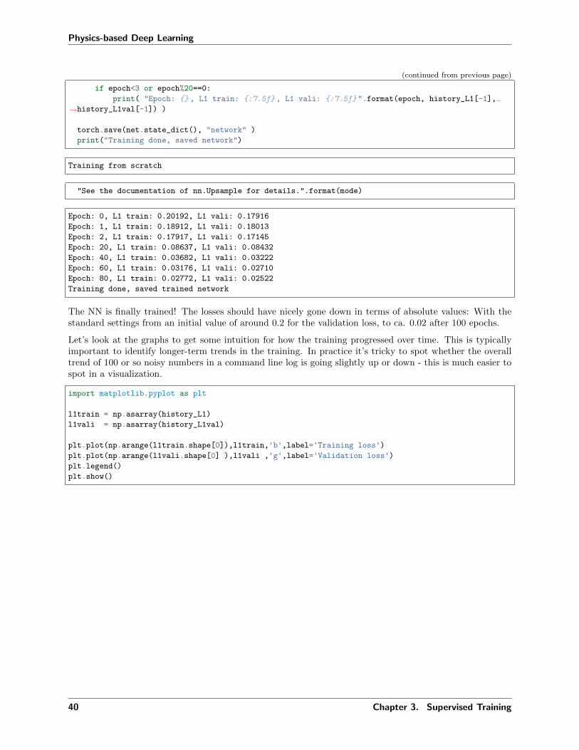
Physics-based Deep Learning
(continued from previous page)
if epoch<3 or epoch%20==0:
print( "Epoch: , L1 train: :7.5f , L1 vali: :7.5f ".format(epoch, history_L1[-1],
→˓history_L1val[-1]) )
torch.save(net.state_dict(), "network" )
print("Training done, saved network")
Training from scratch
"See the documentation of nn.Upsample for details.".format(mode)
Epoch: 0, L1 train: 0.20192, L1 vali: 0.17916
Epoch: 1, L1 train: 0.18912, L1 vali: 0.18013
Epoch: 2, L1 train: 0.17917, L1 vali: 0.17145
Epoch: 20, L1 train: 0.08637, L1 vali: 0.08432
Epoch: 40, L1 train: 0.03682, L1 vali: 0.03222
Epoch: 60, L1 train: 0.03176, L1 vali: 0.02710
Epoch: 80, L1 train: 0.02772, L1 vali: 0.02522
Training done, saved trained network
The NN is finally trained! The losses should have nicely gone down in terms of absolute values: With thestandard settings from an initial value of around 0.2 for the validation loss, to ca. 0.02 after 100 epochs.
Let’s look at the graphs to get some intuition for how the training progressed over time. This is typicallyimportant to identify longer-term trends in the training. In practice it’s tricky to spot whether the overalltrend of 100 or so noisy numbers in a command line log is going slightly up or down - this is much easier tospot in a visualization.
import matplotlib.pyplot as plt
l1train = np.asarray(history_L1)
l1vali = np.asarray(history_L1val)
plt.plot(np.arange(l1train.shape[0]),l1train,'b',label='Training loss')plt.plot(np.arange(l1vali.shape[0] ),l1vali ,'g',label='Validation loss')plt.legend()
plt.show()
40 Chapter 3. Supervised Training

Physics-based Deep Learning
You should see a curve that goes down for ca. 40 epochs, and then starts to flatten out. In the last part,it’s still slowly decreasing, and most importantly, the validation loss is not increasing. This would be acertain sign of overfitting, and something that we should avoid. (Try decreasing the amount of training dataartificially, then you should be able to intentionally cause overfitting.)
3.4.7 Training progress and validation
If you look closely at this graph, you should spot something peculiar: Why is the validation loss lower thanthe training loss? The data is similar to the training data of course, but in a way it’s slightly “tougher”,because the network certainly never received any validation samples during training. It is natural that thevalidation loss slightly deviates from the training loss, but how can the L1 loss be lower for these inputs?
This is a subtlety of the training loop above: it runs a training step first, and the loss for each point inthe graph is measured with the evolving state of the network in an epoch. The network is updated, andafterwards runs through the validation samples. Thus all validation samples are using a state that is definitelydifferent (and hopefully a bit better) than the initial states of the epoch. Hence, the validation loss can beslightly lower.
A general word of caution here: never evaluate your network with training data! That won’t tell youmuch because overfitting is a very common problem. At least use data the network hasn’t seen before, i.e.validation data, and if that looks good, try some more different (at least slightly out-of-distribution) inputs,i.e., test data. The next cell runs the trained network over the validation data, and displays one of themwith the showSbs function.
net.eval()
for i, validata in enumerate(valiLoader, 0):
inputs_curr, targets_curr = validata
inputs.data.copy_(inputs_curr.float())
targets.data.copy_(targets_curr.float())
outputs = net(inputs)
outputs_curr = outputs.data.cpu().numpy()
if i<1: showSbs(targets_curr[0] , outputs_curr[0], title="Validation sample %d "%(i*BATCH_SIZE))
3.4. Supervised training for RANS flows around airfoils 41

Physics-based Deep Learning
"See the documentation of nn.Upsample for details.".format(mode)
Visually, there should at least be a rough resemblance here between input out network output. We’ll savethe more detailed evaluation for the test data, though.
3.4.8 Test evaluation
Now let’s look at actual test samples: In this case we’ll use new airfoil shapes as out-of-distribution (OOD)data. These are shapes that the network never saw in any training samples, and hence it tells us a bit abouthow well the NN generalizes to unseen inputs (the validation data wouldn’t suffice to draw conclusions aboutgeneralization).
We’ll use the same visualization as before, and as indicated by the Bernoulli equation, especially the pressurein the first column is a challenging quantity for the network. Due to it’s cubic scaling w.r.t. the inputfreestream velocity and localized peaks, it is the toughest quantity to infer for the network.
The cell below first downloads a smaller archive with these test data samples, and then runs them throughthe network. The evaluation loop also computes the accumulated L1 error such that we can quantify howwell the network does on the test samples.
if not os.path.isfile('data-airfoils-test.npz'):import urllib.request
url="https://physicsbaseddeeplearning.org/data/data_test.npz"
print("Downloading test data, this should be fast...")
urllib.request.urlretrieve(url, 'data-airfoils-test.npz')
nptfile=np.load('data-airfoils-test.npz')print("Loaded / test samples\n".format(len(nptfile["test_inputs"]),len(nptfile["test_targets
→˓"])))
(continues on next page)
42 Chapter 3. Supervised Training

Physics-based Deep Learning
(continued from previous page)
testdata = DfpDataset(nptfile["test_inputs"],nptfile["test_targets"])
testLoader = torch.utils.data.DataLoader(testdata, batch_size=1, shuffle=False, drop_last=True)
net.eval()
L1t_accum = 0.
for i, validata in enumerate(testLoader, 0):
inputs_curr, targets_curr = validata
inputs.data.copy_(inputs_curr.float())
targets.data.copy_(targets_curr.float())
outputs = net(inputs)
outputs_curr = outputs.data.cpu().numpy()
lossL1t = criterionL1(outputs, targets)
L1t_accum += lossL1t.item()
if i<3: showSbs(targets_curr[0] , outputs_curr[0], title="Test sample %d "%(i))
print("\nAverage test error: ".format( L1t_accum/len(testLoader) ))
Downloading test data, this should be fast...
Loaded 10/10 test samples
"See the documentation of nn.Upsample for details.".format(mode)
Average test error: 0.029000501427799464
3.4. Supervised training for RANS flows around airfoils 43

Physics-based Deep Learning
The average test error with the default settings should be ca. 0.03. As the inputs are normalized, this meansthe average error across all three fields is 3% w.r.t. the maxima of each quantity. This is not too bad fornew shapes, but clearly leaves room for improvement.
Looking at the visualizations, you’ll notice that especially high-pressure peaks and pockets of larger y-
44 Chapter 3. Supervised Training

Physics-based Deep Learning
velocities are missing in the outputs. This is primarily caused by the small network, which does not haveenough resources to reconstruct details.
Nonetheless, we have successfully replaced a fairly sophisticated RANS solver with a very small and fastneural network architecture. It has GPU support “out-of-the-box” (via pytorch), is differentiable, andintroduces an error of only a few per-cent.
3.4.9 Next steps
There are many obvious things to try here (see the suggestions below), e.g. longer training, larger data sets,larger networks etc.
• Experiment with learning rate, dropout, and network size to reduce the error on the test set. Howsmall can you make it with the given training data?
• The setup above uses normalized data. Instead you can recover the original fields by undoing thenormalization to check how well the network does w.r.t. the original quantities.
• As you’ll see, it’s a bit limited here what you can get out of this dataset, head over to the main githubrepo of this project to download larger data sets, or generate own data.
3.5 Discussion of Supervised Approaches
The previous example illustrates that we can quite easily use supervised training to solve complex tasks.The main workload is collecting a large enough dataset of examples. Once that exists, we can train anetwork to approximate the solution manifold sampled by these solutions, and the trained network can giveus predictions very quickly. There are a few important points to keep in mind when using supervised training.
3.5.1 Some things to keep in mind...
Natural starting point
Supervised training is the natural starting point for any DL project. It always, and we really mean alwayshere, makes sense to start with a fully supervised test using as little data as possible. This will be a pureoverfitting test, but if your network can’t quickly converge and give a very good performance on a singleexample, then there’s something fundamentally wrong with your code or data. Thus, there’s no reason tomove on to more complex setups that will make finding these fundamental problems more difficult.
Best practices
To summarize the scattered comments of the previous sections, here’s a set of “golden rules” for setting upa DL project.
• Always start with a 1-sample overfitting test.
• Check how many trainable parameters your network has.
• Slowly increase the amount of training data (and potentially network parameters and depth).
3.5. Discussion of Supervised Approaches 45

Physics-based Deep Learning
• Adjust hyperparameters (especially the learning rate).
• Then introduce other components such as differentiable solvers or adversarial training.
Stability
A nice property of the supervised training is also that it’s very stable. Things won’t get any better when weinclude more complex physical models, or look at more complicated NN architectures.
Thus, again, make sure you can see a nice exponential falloff in your training loss when starting with thesimple overfitting tests. This is a good setup to figure out an upper bound and reasonable range for thelearning rate as the most central hyperparameter. You’ll probably need to reduce it later on, but you shouldat least get a rough estimate of suitable values for 𝜂.
Know your data
All data-driven methods obey the garbage-in-garbage-out principle. Because of this it’s important to workon getting to know the data you are dealing with. While there’s no one-size-fits-all approach for how tobest achieve this, we can strongly recommend to track a broad range of statistics of your data set. A goodstarting point are per quantity mean, standard deviation, min and max values. If some of these containunusual values, this is a first indicator of bad samples in the dataset.
These values can also be easily visualized in terms of histograms, to track down unwanted outliers. A smallnumber of such outliers can easily skew a data set in undesirable ways.
Finally, checking the relationships between different quantities is often a good idea to get some intuition forwhat’s contained in the data set. The next figure gives an example for this step.
Figure2: An example from the airfoil case of the previous section: a visualization of a training data set interms of mean u and v velocity of 2D flow fields. It nicely shows that there are no extreme outliers, butthere are a few entries with relatively low mean u velocity on the left side. A second, smaller data set isshown on top in red, showing that its samples cover the range of mean motions quite well.
46 Chapter 3. Supervised Training
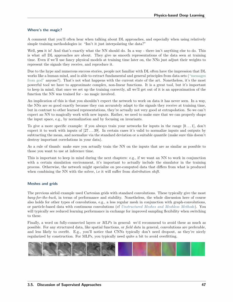
Physics-based Deep Learning
Where’s the magic?
A comment that you’ll often hear when talking about DL approaches, and especially when using relativelysimple training methodologies is: “Isn’t it just interpolating the data?”
Well, yes it is! And that’s exactly what the NN should do. In a way - there isn’t anything else to do. Thisis what all DL approaches are about. They give us smooth representations of the data seen at trainingtime. Even if we’ll use fancy physical models at training time later on, the NNs just adjust their weights torepresent the signals they receive, and reproduce it.
Due to the hype and numerous success stories, people not familiar with DL often have the impression that DLworks like a human mind, and is able to extract fundamental and general principles from data sets (“messagesfrom god” anyone?). That’s not what happens with the current state of the art. Nonetheless, it’s the mostpowerful tool we have to approximate complex, non-linear functions. It is a great tool, but it’s importantto keep in mind, that once we set up the training correctly, all we’ll get out of it is an approximation of thefunction the NN was trained for - no magic involved.
An implication of this is that you shouldn’t expect the network to work on data it has never seen. In a way,the NNs are so good exactly because they can accurately adapt to the signals they receive at training time,but in contrast to other learned representations, they’re actually not very good at extrapolation. So we can’texpect an NN to magically work with new inputs. Rather, we need to make sure that we can properly shapethe input space, e.g., by normalization and by focusing on invariants.
To give a more specific example: if you always train your networks for inputs in the range [0 . . . 1], don’texpect it to work with inputs of [27 . . . 39]. In certain cases it’s valid to normalize inputs and outputs bysubtracting the mean, and normalize via the standard deviation or a suitable quantile (make sure this doesn’tdestroy important correlations in your data).
As a rule of thumb: make sure you actually train the NN on the inputs that are as similar as possible tothose you want to use at inference time.
This is important to keep in mind during the next chapters: e.g., if we want an NN to work in conjunctionwith a certain simulation environment, it’s important to actually include the simulator in the trainingprocess. Otherwise, the network might specialize on pre-computed data that differs from what is producedwhen combining the NN with the solver, i.e it will suffer from distribution shift.
Meshes and grids
The previous airfoil example used Cartesian grids with standard convolutions. These typically give the mostbang-for-the-buck, in terms of performance and stability. Nonetheless, the whole discussion here of coursealso holds for other types of convolutions, e.g., a less regular mesh in conjunction with graph-convolutions,or particle-based data with continuous convolutions (cf Unstructured Meshes and Meshless Methods). Youwill typically see reduced learning performance in exchange for improved sampling flexibility when switchingto these.
Finally, a word on fully-connected layers or MLPs in general: we’d recommend to avoid these as much aspossible. For any structured data, like spatial functions, or field data in general, convolutions are preferable,and less likely to overfit. E.g., you’ll notice that CNNs typically don’t need dropout, as they’re nicelyregularized by construction. For MLPs, you typically need quite a bit to avoid overfitting.
3.5. Discussion of Supervised Approaches 47

Physics-based Deep Learning
3.5.2 Supervised training in a nutshell
To summarize, supervised training has the following properties.
Pros:
• Very fast training.
• Stable and simple.
• Great starting point.
Con:
• Lots of data needed.
• Sub-optimal performance, accuracy and generalization.
• Interactions with external “processes” (such as embedding into a solver) are difficult.
The next chapters will explain how to alleviate these shortcomings of supervised training. First, we’ll lookat bringing model equations into the picture via soft-constraints, and afterwards we’ll revisit the challengesof bringing together numerical simulations and learned approaches.
48 Chapter 3. Supervised Training

Part II
Physical Losses
49


CHAPTER
FOUR
PHYSICAL LOSS TERMS
The supervised setting of the previous sections can quickly yield approximate solutions with a fairly simpletraining process. However, what’s quite sad to see here is that we only use physical models and numericalmethods as an “external” tool to produce a big pile of data .
We as humans have a lot of knowledge about how to describe physical processes mathematically. As thefollowing chapters will show, we can improve the training process by guiding it with our human knowledgeof physics.
Figure1: Physical losses typically combine a supervised loss with a combination of derivatives from the neuralnetwork.
4.1 Using physical models
Given a PDE for u(x, 𝑡) with a time evolution, we can typically express it in terms of a function ℱ of thederivatives of u via
u𝑡 = ℱ(u𝑥,u𝑥𝑥, ...u𝑥𝑥...𝑥),
where the x subscripts denote spatial derivatives with respect to one of the spatial dimensions of higher andhigher order (this can of course also include mixed derivatives with respect to different axes). ∖mathbfu tdenotes the changes over time.
In this context, we can approximate the unknown u itself with a neural network. If the approximation,which we call u, is accurate, the PDE should be satisfied naturally. In other words, the residual R shouldbe equal to zero:
𝑅 = u𝑡 −ℱ(u𝑥,u𝑥𝑥, ...u𝑥𝑥...𝑥) = 0.
51

Physics-based Deep Learning
This nicely integrates with the objective for training a neural network: we can train for minimizing thisresidual in combination with direct loss terms. Similar to before, we can make use of sample solutions[𝑥0, 𝑦0], ...[𝑥𝑛, 𝑦𝑛] for u with u(x) = 𝑦. This is typically important, as most practical PDEs we encounter donot have unique solutions unless initial and boundary conditions are specified. Hence, if we only consider 𝑅we might get solutions with random offset or other undesirable components. The supervised sample pointstherefore help to pin down the solution in certain places. Now our training objective becomes
arg min𝜃 𝛼0
∑𝑖
(𝑓(𝑥𝑖; 𝜃) − 𝑦𝑖
)2+ 𝛼1𝑅(𝑥𝑖), (1)
where 𝛼0,1 denote hyperparameters that scale the contribution of the supervised term and the residual term,respectively. We could of course add additional residual terms with suitable scaling factors here.
It is instructive to note what the two different terms in equation (1) mean: The first term is a conventional,supervised L2-loss. If we were to optimize only this loss, our network would learn to approximate the trainingsamples well, but might average multiple modes in the solutions, and do poorly in regions in between thesample points. If we, instead, were to optimize only the second term (the physical residual), our neuralnetwork might be able to locally satisfy the PDE, but still could produce solutions that are still far awayfrom our training data. This can happen due to “null spaces” in the solutions, i.e., different solutions thatall satisfy the residuals. Therefore, we optimize both objectives simultaneously such that, in the best case,the network learns to approximate the specific solutions of the training data while still capturing knowledgeabout the underlying PDE.
Note that, similar to the data samples used for supervised training, we have no guarantees that the residualterms 𝑅 will actually reach zero during training. The non-linear optimization of the training process willminimize the supervised and residual terms as much as possible, but there is no guarantee. Large, non-zeroresidual contributions can remain. We’ll look at this in more detail in the upcoming code example, for nowit’s important to remember that physical constraints in this way only represent soft-constraints, withoutguarantees of minimizing these constraints.
4.2 Neural network derivatives
In order to compute the residuals at training time, it would be possible to store the unknowns of u on acomputational mesh, e.g., a grid, and discretize the equations of 𝑅 there. This has a fairly long “tradition”in DL, and was proposed by Tompson et al. [TSSP17] early on.
A popular variant of employing physical soft-constraints [RK18] instead uses fully connected NNs to representu. This has some interesting pros and cons that we’ll outline in the following, and we will also focus on it inthe following code examples and comparisons.
The central idea here is that the aforementioned general function 𝑓 that we’re after in our learning problemscan also be used to obtain a representation of a physical field, e.g., a field u that satisfies 𝑅 = 0. This meansu(x) will be turned into u(x, 𝜃) where we choose the NN parameters 𝜃 such that a desired u is representedas precisely as possible.
One nice side effect of this viewpoint is that NN representations inherently support the calculation of deriva-tives. The derivative 𝜕𝑓/𝜕𝜃 was a key building block for learning via gradient descent, as explained inOverview . Now, we can use the same tools to compute spatial derivatives such as 𝜕u/𝜕𝑥, Note that abovefor 𝑅 we’ve written this derivative in the shortened notation as u𝑥. For functions over time this of coursealso works for 𝜕u/𝜕𝑡, i.e. u𝑡 in the notation above.
Thus, for some generic 𝑅, made up of u𝑡 and u𝑥 terms, we can rely on the backpropagation algorithm of DLframeworks to compute these derivatives once we have a NN that represents u. Essentially, this gives us afunction (the NN) that receives space and time coordinates to produce a solution for u. Hence, the input istypically quite low-dimensional, e.g., 3+1 values for a 3D case over time, and often produces a scalar value
52 Chapter 4. Physical Loss Terms
Physics-based Deep Learning
or a spatial vector. Due to the lack of explicit spatial sampling points, an MLP, i.e., fully-connected NN isthe architecture of choice here.
To pick a simple example, Burgers equation in 1D, 𝜕𝑢𝜕𝑡 +𝑢∇𝑢 = 𝜈∇·∇𝑢 , we can directly formulate a loss term
𝑅 = 𝜕𝑢𝜕𝑡 +𝑢𝜕𝑢
𝜕𝑥 −𝜈 𝜕2𝑢𝜕𝑥2 𝑢 that should be minimized as much as possible at training time. For each of the terms,
e.g. 𝜕𝑢𝜕𝑥 , we can simply query the DL framework that realizes 𝑢 to obtain the corresponding derivative. For
higher order derivatives, such as 𝜕2𝑢𝜕𝑥2 , we can simply query the derivative function of the framework multiple
times. In the following section, we’ll give a specific example of how that works in tensorflow.
4.3 Summary so far
The approach above gives us a method to include physical equations into DL learning as a soft-constraint:the residual loss. Typically, this setup is suitable for inverse problems, where we have certain measurementsor observations for which we want to find a PDE solution. Because of the high cost of the reconstruction(to be demonstrated in the following), the solution manifold shouldn’t be overly complex. E.g., it is notpossible to capture a wide range of solutions, such as with the previous supervised airfoil example, with sucha physical residual loss.
4.3. Summary so far 53

Physics-based Deep Learning
54 Chapter 4. Physical Loss Terms

CHAPTER
FIVE
BURGERS OPTIMIZATION WITH A PHYSICS-INFORMED NN
To illustrate how the physics-informed losses work, let’s consider a reconstruction task as an inverse problemexample. We’ll use Burgers equation 𝜕𝑢
𝜕𝑡 + 𝑢∇𝑢 = 𝜈∇ · ∇𝑢 as a simple yet non-linear equation in 1D, forwhich we have a series of observations at time 𝑡 = 0.5. The solution should fulfill the residual formulationfor Burgers equation and match the observations. In addition, let’s impose Dirichlet boundary conditions𝑢 = 0 at the sides of our computational domain, and define the solution in the time interval 𝑡 ∈ [0, 1].
Note that similar to the previous forward simulation example, we will still be sampling the solution with 128points (𝑛 = 128), but now we have a discretization via the NN. So we could also sample points in betweenwithout having to explicitly choose a basis function for interpolation. The discretization via the NN nowinternally determines how to use its degrees of freedom to arrange the activation functions as basis functions.So we have no direct control over the reconstruction. [run in colab]
5.1 Formulation
In terms of the 𝑥, 𝑦* notation from Models and Equations and the previous section, this reconstructionproblem means we are solving
arg min𝜃
∑𝑖
(𝑓(𝑥𝑖; 𝜃) − 𝑦*𝑖 )2 + 𝑅(𝑥𝑖),
where 𝑥 and 𝑦* are solutions of 𝑢 at different locations in space and time. As we’re dealing with a 1D velocity,𝑥, 𝑦* ∈ R. They both represent two-dimensional solutions 𝑥(𝑝𝑖, 𝑡𝑖) and 𝑦*(𝑝𝑖, 𝑡𝑖) for a spatial coordinate 𝑝𝑖and a time 𝑡𝑖, where the index 𝑖 sums over a set of chosen 𝑝𝑖, 𝑡𝑖 locations at which we evaluate the PDE andthe approximated solutions. Thus 𝑦* denotes a reference 𝑢 for 𝒫 being Burgers equation, which 𝑥 shouldapproximate as closely as possible. Thus our neural network representation of 𝑥 will receive 𝑝, 𝑡 as input toproduce a velocity solution at the specified position.
The residual function 𝑅 above collects additional evaluations of 𝑓(; 𝜃) and its derivatives to formulate theresidual for 𝒫. This approach - using derivatives of a neural network to compute a PDE residual - istypically called a physics-informed approach, yielding a physics-informed neural network (PINN) to representa solution for the inverse reconstruction problem.
Thus, in the formulation above, 𝑅 should simply converge to zero above. We’ve omitted scaling factors inthe objective function for simplicity. Note that, effectively, we’re only dealing with individual point samplesof a single solution 𝑢 for 𝒫 here.
55

Physics-based Deep Learning
5.2 Preliminaries
Let’s just load phiflow with the tensorflow backend for now, and initialize the random sampling. (Note: thisexample uses an older version 1.5.1 of phiflow.)
!pip install --upgrade --quiet git+https://github.com/tum-pbs/[email protected]
from phi.tf.flow import *
import numpy as np
#rnd = TF_BACKEND # for phiflow: sample different points in the domain each iteration
rnd = math.choose_backend(1) # use same random points for all iterations
We’re importing phiflow here, but we won’t use it to compute a solution to the PDE as in Simple ForwardSimulation of Burgers Equation with phiflow . Instead, we’ll use the derivatives of an NN (as explained inthe previous section) to set up a loss formulation for training.
Next, we set up a simple NN with 8 fully connected layers and tanh activations with 20 units each.
We’ll also define the boundary tx function which gives an array of constraints for the solution (all for = 0.5in this example), and the open boundary function which stores constraints for 𝑥 = ±1 being 0.
def network(x, t):
""" Dense neural network with 8 hidden layers and 3021 parameters in total.
Parameters will only be allocated once (auto reuse).
"""
y = math.stack([x, t], axis=-1)
for i in range(8):
y = tf.layers.dense(y, 20, activation=tf.math.tanh, name='layer%d ' % i, reuse=tf.AUTO_
→˓REUSE)
return tf.layers.dense(y, 1, activation=None, name='layer_out', reuse=tf.AUTO_REUSE)
def boundary_tx(N):
x = np.linspace(-1,1,128)
# precomputed solution from forward simulation:
u = np.asarray( [0.008612174447657694, 0.02584669669548606, 0.043136357266407785 ... ] );
t = np.asarray(rnd.ones_like(x)) * 0.5
perm = np.random.permutation(128)
return (x[perm])[0:N], (t[perm])[0:N], (u[perm])[0:N]
def _ALT_t0(N): # alternative, impose original initial state at t=0
x = rnd.random_uniform([N], -1, 1)
t = rnd.zeros_like(x)
u = - math.sin(np.pi * x)
return x, t, u
def open_boundary(N):
t = rnd.random_uniform([N], 0, 1)
x = math.concat([math.zeros([N//2]) + 1, math.zeros([N//2]) - 1], axis=0)
u = math.zeros([N])
return x, t, u
Most importantly, we can now also construct the residual loss function f that we’d like to minimize in orderto guide the NN to retrieve a solution for our model equation. As can be seen in the equation at the top,we need derivatives w.r.t. 𝑡, 𝑥 and a second derivative for 𝑥. The first three lines of f below do just that.
Afterwards, we simply combine the derivates to form Burgers equation. Here we make use of phiflow’sgradient function:
56 Chapter 5. Burgers Optimization with a Physics-Informed NN

Physics-based Deep Learning
def f(u, x, t):
""" Physics-based loss function with Burgers equation """
u_t = gradients(u, t)
u_x = gradients(u, x)
u_xx = gradients(u_x, x)
return u_t + u*u_x - (0.01 / np.pi) * u_xx
Next, let’s set up the sampling points in the inner domain, such that we can compare the solution with theprevious forward simulation in phiflow.
The next cell allocates two tensors: grid x will cover the size of our domain, i.e., the -1 to 1 range, with 128cells, while grid t will sample the time interval [0, 1] with 33 time stamps.
The last math.expand dims() call simply adds another batch dimension, so that the resulting tensor iscompatible with the following examples.
N=128
grids_xt = np.meshgrid(np.linspace(-1, 1, N), np.linspace(0, 1, 33), indexing='ij')grid_x, grid_t = [tf.convert_to_tensor(t, tf.float32) for t in grids_xt]
# create 4D tensor with batch and channel dimensions in addition to space and time
# in this case gives shape=(1, N, 33, 1)
grid_u = math.expand_dims(network(grid_x, grid_t))
Instructions for updating:
Use keras.layers.Dense instead.
Instructions for updating:
Please use `layer.__call__` method instead.
Now, grid u contains a full graph to evaluate our NN at 128 × 33 positions, and returns the results in a[1, 128, 33, 1] array once we run it through session.run. Let’s give this a try: we can initialize a TF session,evaluate grid u and show it in an image, just like the phiflow solution we computed previously.
(Note, we’ll use the show state as in Simple Forward Simulation of Burgers Equation with phiflow . Hence,the x axis does not show actual simulation time, but is showing 32 steps “blown” up by a factor of 16 tomake the changes over time easier to see in the image.)
import pylab as plt
print("Size of grid_u: "+format(grid_u.shape))
session = Session(None)
session.initialize_variables()
def show_state(a, title):
for i in range(4): a = np.concatenate( [a,a] , axis=3)
a = np.reshape( a, [a.shape[1],a.shape[2]*a.shape[3]] )
fig, axes = plt.subplots(1, 1, figsize=(16, 5))
im = axes.imshow(a, origin='upper', cmap='inferno')plt.colorbar(im) ; plt.xlabel('time'); plt.ylabel('x'); plt.title(title)
print("Randomly initialized network state:")
show_state(session.run(grid_u),"Uninitialized NN")
Size of grid_u: (1, 128, 33, 1)
Randomly initialized network state:
5.2. Preliminaries 57
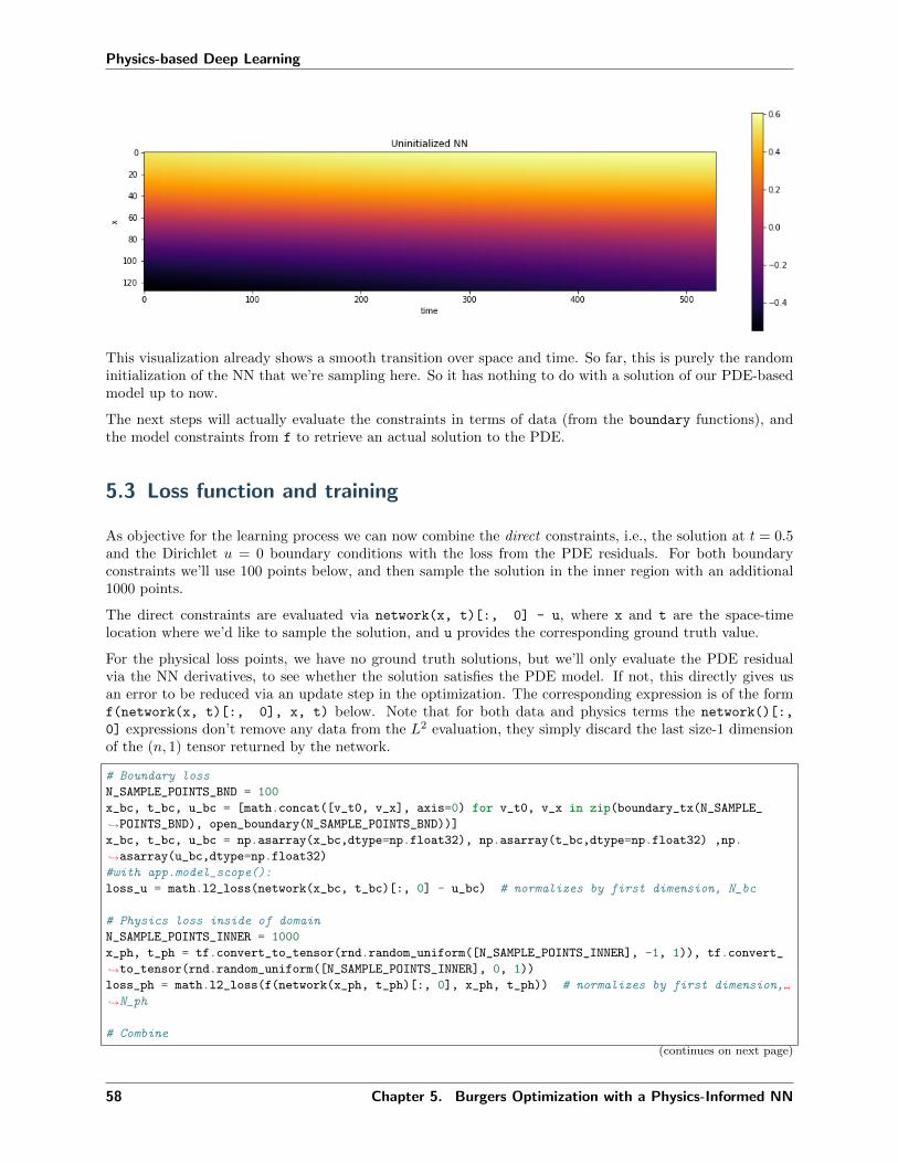
Physics-based Deep Learning
This visualization already shows a smooth transition over space and time. So far, this is purely the randominitialization of the NN that we’re sampling here. So it has nothing to do with a solution of our PDE-basedmodel up to now.
The next steps will actually evaluate the constraints in terms of data (from the boundary functions), andthe model constraints from f to retrieve an actual solution to the PDE.
5.3 Loss function and training
As objective for the learning process we can now combine the direct constraints, i.e., the solution at 𝑡 = 0.5and the Dirichlet 𝑢 = 0 boundary conditions with the loss from the PDE residuals. For both boundaryconstraints we’ll use 100 points below, and then sample the solution in the inner region with an additional1000 points.
The direct constraints are evaluated via network(x, t)[:, 0] - u, where x and t are the space-timelocation where we’d like to sample the solution, and u provides the corresponding ground truth value.
For the physical loss points, we have no ground truth solutions, but we’ll only evaluate the PDE residualvia the NN derivatives, to see whether the solution satisfies the PDE model. If not, this directly gives usan error to be reduced via an update step in the optimization. The corresponding expression is of the formf(network(x, t)[:, 0], x, t) below. Note that for both data and physics terms the network()[:,
0] expressions don’t remove any data from the 𝐿2 evaluation, they simply discard the last size-1 dimensionof the (𝑛, 1) tensor returned by the network.
# Boundary loss
N_SAMPLE_POINTS_BND = 100
x_bc, t_bc, u_bc = [math.concat([v_t0, v_x], axis=0) for v_t0, v_x in zip(boundary_tx(N_SAMPLE_
→˓POINTS_BND), open_boundary(N_SAMPLE_POINTS_BND))]
x_bc, t_bc, u_bc = np.asarray(x_bc,dtype=np.float32), np.asarray(t_bc,dtype=np.float32) ,np.
→˓asarray(u_bc,dtype=np.float32)
#with app.model_scope():
loss_u = math.l2_loss(network(x_bc, t_bc)[:, 0] - u_bc) # normalizes by first dimension, N_bc
# Physics loss inside of domain
N_SAMPLE_POINTS_INNER = 1000
x_ph, t_ph = tf.convert_to_tensor(rnd.random_uniform([N_SAMPLE_POINTS_INNER], -1, 1)), tf.convert_
→˓to_tensor(rnd.random_uniform([N_SAMPLE_POINTS_INNER], 0, 1))
loss_ph = math.l2_loss(f(network(x_ph, t_ph)[:, 0], x_ph, t_ph)) # normalizes by first dimension,
→˓N_ph
# Combine
(continues on next page)
58 Chapter 5. Burgers Optimization with a Physics-Informed NN

Physics-based Deep Learning
(continued from previous page)
ph_factor = 1.
loss = loss_u + ph_factor * loss_ph # allows us to control the relative influence of loss_ph
optim = tf.train.GradientDescentOptimizer(learning_rate=0.02).minimize(loss)
#optim = tf.train.AdamOptimizer(learning_rate=0.001).minimize(loss) # alternative, but not much
→˓benefit here
The code above just initializes the evaluation of the loss, we still didn’t do any optimization steps, but we’refinally in a good position to get started with this.
Despite the simple equation, the convergence is typically very slow. The iterations themselves are fast tocompute, but this setup needs a lot of iterations. To keep the runtime in a reasonable range, we only do 10kiterations by default below (ITERS). You can increase this value to get better results.
session.initialize_variables()
import time
start = time.time()
ITERS = 10000
for optim_step in range(ITERS+1):
_, loss_value = session.run([optim, loss])
if optim_step<3 or optim_step%1000==0:
print('Step %d , loss: %f ' % (optim_step,loss_value))
#show_state(grid_u)
end = time.time()
print("Runtime :.2f s".format(end-start))
Step 0, loss: 0.108430
Step 1, loss: 0.103907
Step 2, loss: 0.100539
Step 1000, loss: 0.057177
Step 2000, loss: 0.053230
Step 3000, loss: 0.049326
Step 4000, loss: 0.046316
Step 5000, loss: 0.044153
Step 6000, loss: 0.041827
Step 7000, loss: 0.039517
Step 8000, loss: 0.037237
Step 9000, loss: 0.035256
Step 10000, loss: 0.033931
Runtime 110.15s
The training can take a significant amount of time, around 2 minutes on a typical notebook, but at least theerror goes down significantly (roughly from around 0.2 to ca. 0.03), and the network seems to successfullyconverge to a solution.
Let’s show the reconstruction of the network, by evaluating the network at the centers of a regular grid,so that we can show the solution as an image. Note that this is actually fairly expensive, we have to runthrough the whole network with a few thousand weights for all of the 128 × 32 sampling points in the grid.
It looks pretty good on first sight, though. There’s been a very noticeable change compared to the randominitialization shown above:
show_state(session.run(grid_u),"After Training")
5.3. Loss function and training 59

Physics-based Deep Learning
5.4 Evaluation
Let’s compare solution in a bit more detail. Here are the actual sample points used for constraining thesolution (at time step 16, 𝑡 = 1/2) shown in gray, versus the reconstructed solution in blue:
u = session.run(grid_u)
# solution is imposed at t=1/2 , which is 16 in the array
BC_TX = 16
uT = u[0,:,BC_TX,0]
fig = plt.figure().gca()
fig.plot(np.linspace(-1,1,len(uT)), uT, lw=2, color='blue', label="NN")
fig.scatter(x_bc[0:100], u_bc[0:100], color='gray', label="Reference")
plt.title("Comparison at t=1/2")
plt.xlabel('x'); plt.ylabel('u'); plt.legend()
<matplotlib.legend.Legend at 0x7f84721c3fd0>
60 Chapter 5. Burgers Optimization with a Physics-Informed NN

Physics-based Deep Learning
Not too bad at the sides of the domain (the Dirichlet boundary conditions 𝑢 = 0 are fulfilled), but the shockin the center (at 𝑥 = 0) is not well represented.
Let’s check how well the initial state at 𝑡 = 0 was reconstructed. That’s the most interesting, and toughestpart of the problem (the rest basically follows from the model equation and boundary conditions, given thefirst state).
It turns out that the accuracy of the initial state is actually not that good: the blue curve from the PINNis quite far away from the constraints via the reference data (shown in gray)... The solution will get betterwith larger number of iterations, but it requires a surprisingly large number of iterations for this fairly simplecase.
# ground truth solution at t0
t0gt = np.asarray( [ [-math.sin(np.pi * x) * 1.] for x in np.linspace(-1,1,N)] )
velP0 = u[0,:,0,0]
fig = plt.figure().gca()
fig.plot(np.linspace(-1,1,len(velP0)), velP0, lw=2, color='blue', label="NN")
fig.plot(np.linspace(-1,1,len(t0gt)), t0gt, lw=2, color='gray', label="Reference")
plt.title("Comparison at t=0")
plt.xlabel('x'); plt.ylabel('u'); plt.legend()
<matplotlib.legend.Legend at 0x7f847223da60>
5.4. Evaluation 61
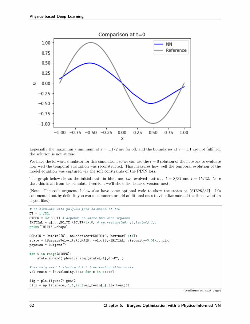
Physics-based Deep Learning
Especially the maximum / minimum at 𝑥 = ±1/2 are far off, and the boundaries at 𝑥 = ±1 are not fulfilled:the solution is not at zero.
We have the forward simulator for this simulation, so we can use the 𝑡 = 0 solution of the network to evaluatehow well the temporal evaluation was reconstructed. This measures how well the temporal evolution of themodel equation was captured via the soft constraints of the PINN loss.
The graph below shows the initial state in blue, and two evolved states at 𝑡 = 8/32 and 𝑡 = 15/32. Notethat this is all from the simulated version, we’ll show the learned version next.
(Note: The code segments below also have some optional code to show the states at [STEPS//4]. It’scommented out by default, you can uncomment or add additional ones to visualize more of the time evolutionif you like.)
# re-simulate with phiflow from solution at t=0
DT = 1./32.
STEPS = 32-BC_TX # depends on where BCs were imposed
INITIAL = u[...,BC_TX:(BC_TX+1),0] # np.reshape(u0, [1,len(u0),1])
print(INITIAL.shape)
DOMAIN = Domain([N], boundaries=PERIODIC, box=box[-1:1])
state = [BurgersVelocity(DOMAIN, velocity=INITIAL, viscosity=0.01/np.pi)]
physics = Burgers()
for i in range(STEPS):
state.append( physics.step(state[-1],dt=DT) )
# we only need "velocity.data" from each phiflow state
vel_resim = [x.velocity.data for x in state]
fig = plt.figure().gca()
pltx = np.linspace(-1,1,len(vel_resim[0].flatten()))
(continues on next page)
62 Chapter 5. Burgers Optimization with a Physics-Informed NN

Physics-based Deep Learning
(continued from previous page)
fig.plot(pltx, vel_resim[ 0].flatten(), lw=2, color='blue', label="t=0")
#fig.plot(pltx, vel_resim[STEPS//4].flatten(), lw=2, color='green', label="t=0.125")
fig.plot(pltx, vel_resim[STEPS//2].flatten(), lw=2, color='cyan', label="t=0.25")
fig.plot(pltx, vel_resim[STEPS-1].flatten(), lw=2, color='purple',label="t=0.5")#fig.plot(pltx, t0gt, lw=2, color='gray', label="t=0 Reference") # optionally show GT, compare to
→˓blue
plt.title("Resimulated u from solution at t=0")
plt.xlabel('x'); plt.ylabel('u'); plt.legend()
(1, 128, 1)
<matplotlib.legend.Legend at 0x7f84722de760>
And here is the PINN output from u at the same time steps:
velP = [u[0,:,x,0] for x in range(33)]
print(velP[0].shape)
fig = plt.figure().gca()
fig.plot(pltx, velP[BC_TX+ 0].flatten(), lw=2, color='blue', label="t=0")
#fig.plot(pltx, velP[BC_TX+STEPS//4].flatten(), lw=2, color='green', label="t=0.125")
fig.plot(pltx, velP[BC_TX+STEPS//2].flatten(), lw=2, color='cyan', label="t=0.25")
fig.plot(pltx, velP[BC_TX+STEPS-1].flatten(), lw=2, color='purple',label="t=0.5")plt.title("NN Output")
plt.xlabel('x'); plt.ylabel('u'); plt.legend()
(128,)
5.4. Evaluation 63

Physics-based Deep Learning
<matplotlib.legend.Legend at 0x7f8470cfb1f0>
Judging via eyeball norm, these two versions of 𝑢 look quite similar, but not surprisingly the errors growover time and there are significant differences. Especially the steepening of the solution near the shock at𝑥 = 0 is not “captured” well. It’s a bit difficult to see in these two graphs, though, let’s quantify the errorand show the actual difference:
error = np.sum( np.abs( np.asarray(vel_resim[0:16]).flatten() - np.asarray(velP[BC_TX:BC_
→˓TX+STEPS]).flatten() )) / (STEPS*N)
print("Mean absolute error for re-simulation across steps: :7.5f ".format(STEPS,error))
fig = plt.figure().gca()
fig.plot(pltx, (vel_resim[0 ].flatten()-velP[BC_TX ].flatten()), lw=2, color='blue',→˓ label="t=5")
fig.plot(pltx, (vel_resim[STEPS//4].flatten()-velP[BC_TX+STEPS//4].flatten()), lw=2, color='green',→˓ label="t=0.625")
fig.plot(pltx, (vel_resim[STEPS//2].flatten()-velP[BC_TX+STEPS//2].flatten()), lw=2, color='cyan',→˓ label="t=0.75")
fig.plot(pltx, (vel_resim[STEPS-1 ].flatten()-velP[BC_TX+STEPS-1 ].flatten()), lw=2, color='purple→˓',label="t=1")plt.title("u Error")
plt.xlabel('x'); plt.ylabel('MAE'); plt.legend()
Mean absolute error for re-simulation across 16 steps: 0.01067
<matplotlib.legend.Legend at 0x7f8472550e50>
64 Chapter 5. Burgers Optimization with a Physics-Informed NN

Physics-based Deep Learning
The code above will compute a mean absolute error of ca. 1.5 ·10−2 between ground truth re-simulation andthe PINN evolution, which is significant for the value range of the simulation.
And for comparison with the forward simulation and following cases, here are also all steps over time witha color map.
# show re-simulated solution again as full image over time
sn = np.concatenate(vel_resim, axis=-1)
sn = np.reshape(sn, list(sn.shape)+[1] ) # print(sn.shape)
show_state(sn,"Re-simulated u")
Next, we’ll store the full solution over the course of the 𝑡 = 0 . . . 1 time interval, so that we can compare it
5.4. Evaluation 65

Physics-based Deep Learning
later on to the full solution from a regular forward solve and compare it to the differential physics solution.
Thus, stay tuned for the full evaluation and the comparison. This will follow in Burgers Optimization witha Differentiable Physics Gradient , after we’ve discussed the details of how to run the differential physicsoptimization.
vels = session.run(grid_u) # special for showing NN results, run through TF
vels = np.reshape( vels, [vels.shape[1],vels.shape[2]] )
# save for comparison with other methods
import os; os.makedirs("./temp",exist_ok=True)
np.savez_compressed("./temp/burgers-pinn-solution.npz",vels) ; print("Vels array shape:
→˓"+format(vels.shape))
Vels array shape: (128, 33)
5.5 Next steps
This setup is just a starting point for PINNs and physical soft-constraints, of course. The parameters ofthe setup were chosen to run relatively quickly. As we’ll show in the next sections, the behavior of such aninverse solve can be improved substantially by a tighter integration of solver and learning.
The solution of the PINN setup above can also directly be improved, however. E.g., try to:
• Adjust parameters of the training to further decrease the error without making the solution diverge.
• Adapt the NN architecture for further improvements (keep track of the weight count, though).
• Activate a different optimizer, and observe the change in behavior (this typically requires adjustingthe learning rate). Note that the more complex optimizers don’t necessarily do better in this relativelysimple example.
• Or modify the setup to make the test case more interesting: e.g., move the boundary conditions to alater point in simulation time, to give the reconstruction a larger time interval to reconstruct.
66 Chapter 5. Burgers Optimization with a Physics-Informed NN

CHAPTER
SIX
DISCUSSION OF PHYSICAL SOFT-CONSTRAINTS
The good news so far is - we have a DL method that can include physical laws in the form of soft constraintsby minimizing residuals. However, as the very simple previous example illustrates, this is just a conceptualstarting point.
On the positive side, we can leverage DL frameworks with backpropagation to compute the derivatives of themodel. At the same time, this puts us at the mercy of the learned representation regarding the reliabilityof these derivatives. Also, each derivative requires backpropagation through the full network, which can bevery expensive. Especially so for higher-order derivatives.
And while the setup is relatively simple, it is generally difficult to control. The NN has flexibility to refinethe solution by itself, but at the same time, tricks are necessary when it doesn’t focus on the right regionsof the solution.
6.1 Is it “Machine Learning”?
One question that might also come to mind at this point is: can we really call it machine learning? Ofcourse, such denomination questions are superficial - if an algorithm is useful, it doesn’t matter what nameit has. However, here the question helps to highlight some important properties that are typically associatedwith algorithms from fields like machine learning or optimization.
One main reason not to call these physical constraints machine learning (ML), is that the positions wherewe test and constrain the solution are the final positions we are interested in. As such, there is no realdistinction between training, validation and (out of distribution) test sets. Computing the solution for aknown and given set of samples is much more akin to classical optimization, where inverse problems like theprevious Burgers example stem from.
For machine learning, we typically work under the assumption that the final performance of our model willbe evaluated on a different, potentially unknown set of inputs. The test data should usually capture suchout of distribution (OOD) behavior, so that we can make estimates about how well our model will generalizeto “real-world” cases that we will encounter when we deploy it into an application.
In contrast, for the PINN training as described here, we reconstruct a single solution in a known and givenspace-time region. As such, any samples from this domain follow the same distribution and hence don’treally represent test or OOD sampes. As the NN directly encodes the solution, there is also little hope thatit will yield different solutions, or perform well outside of the training distribution. If we’re interested in adifferent solution, we most likely have to start training the NN from scratch.
67

Physics-based Deep Learning
6.2 Summary
Thus, the physical soft constraints allow us to encode solutions to PDEs with the tools of NNs. An inherentdrawback of this approach is that it yields single solutions, and that it does not combine with traditionalnumerical techniques well. E.g., the learned representation is not suitable to be refined with a classicaliterative solver such as the conjugate gradient method.
This means many powerful techniques that were developed in the past decades cannot be used in this context.Bringing these numerical methods back into the picture will be one of the central goals of the next sections.
Pro:
• Uses physical model.
• Derivatives can be conveniently computed via backpropagation.
Con:
• Quite slow ...
• Physical constraints are enforced only as soft constraints.
• Largely incompatible with classical numerical methods.
• Accuracy of derivatives relies on learned representation.
Next, let’s look at how we can leverage numerical methods to improve the DL accuracy and efficiency bymaking use of differentiable solvers.
68 Chapter 6. Discussion of Physical Soft-Constraints

Part III
Differentiable Physics
69


CHAPTER
SEVEN
INTRODUCTION TO DIFFERENTIABLE PHYSICS
As a next step towards a tighter and more generic combination of deep learning methods and physicalsimulations we will target incorporating differentiable simulations into the learning process. In the following,we’ll shorten that to “differentiable physics” (DP).
The central goal of these methods is to use existing numerical solvers, and equip them with functionality tocompute gradients with respect to their inputs. Once this is realized for all operators of a simulation, we canleverage the autodiff functionality of DL frameworks with backpropagation to let gradient information flowfrom from a simulator into an NN and vice versa. This has numerous advantages such as improved learningfeedback and generalization, as we’ll outline below.
In contrast to physics-informed loss functions, it also enables handling more complex solution manifoldsinstead of single inverse problems. E.g., instead of using deep learning to solve single inverse problems asin the previous chapter, differentiable physics can be used to train NNs that learn to solve larger classes ofinverse problems very efficiently.
Figure1: Training with differentiable physics means that a chain of differentiable operators provide directionsin the form of gradients to steer the learning process.
71

Physics-based Deep Learning
7.1 Differentiable operators
With the DP direction we build on existing numerical solvers. I.e., the approach is strongly relying on thealgorithms developed in the larger field of computational methods for a vast range of physical effects inour world. To start with, we need a continuous formulation as model for the physical effect that we’d liketo simulate - if this is missing we’re in trouble. But luckily, we can tap into existing collections of modelequations and established methods for discretizing continuous models.
Let’s assume we have a continuous formulation 𝒫*(x, 𝜈) of the physical quantity of interest u(x, 𝑡) : R𝑑 ×R+ → R𝑑, with model parameters 𝜈 (e.g., diffusion, viscosity, or conductivity constants). The component ofu will be denoted by a numbered subscript, i.e., u = (𝑢1, 𝑢2, . . . , 𝑢𝑑)𝑇 .
Typically, we are interested in the temporal evolution of such a system. Discretization yields a formulation𝒫(x, 𝜈) that we can re-arrange to compute a future state after a time step ∆𝑡. The state at 𝑡 + ∆𝑡 iscomputed via sequence of operations 𝒫1,𝒫2 . . .𝒫𝑚 such that u(𝑡 + ∆𝑡) = 𝒫1 ∘ 𝒫2 ∘ . . .𝒫𝑚(u(𝑡), 𝜈), where ∘denotes function decomposition, i.e. 𝑓(𝑔(𝑥)) = 𝑓 ∘ 𝑔(𝑥).
Note: In order to integrate this solver into a DL process, we need to ensure that every operator 𝒫𝑖 providesa gradient w.r.t. its inputs, i.e. in the example above 𝜕𝒫𝑖/𝜕u.
Note that we typically don’t need derivatives for all parameters of 𝒫(x, 𝜈), e.g., we omit 𝜈 in the following,assuming that this is a given model parameter with which the NN should not interact. Naturally, it can varywithin the solution manifold that we’re interested in, but 𝜈 will not be the output of an NN representation.If this is the case, we can omit providing 𝜕𝒫𝑖/𝜕𝜈 in our solver. However, the following learning processnaturally transfers to including 𝜈 as a degree of freedom.
7.2 Jacobians
As u is typically a vector-valued function, 𝜕𝒫𝑖/𝜕u denotes a Jacobian matrix 𝐽 rather than a single value:
𝜕𝒫𝑖
𝜕u=
⎡⎢⎣𝜕𝒫𝑖,1/𝜕𝑢1 · · · 𝜕𝒫𝑖,1/𝜕𝑢𝑑
...𝜕𝒫𝑖,𝑑/𝜕𝑢1 · · · 𝜕𝒫𝑖,𝑑/𝜕𝑢𝑑
⎤⎥⎦where, as above, 𝑑 denotes the number of components in u. As 𝒫 maps one value of u to another, theJacobian is square and symmetric here. Of course this isn’t necessarily the case for general model equations,but non-square Jacobian matrices would not cause any problems for differentiable simulations.
In practice, we can rely on the reverse mode differentiation that all modern DL frameworks provide, andfocus on computing a matrix vector product of the Jacobian transpose with a vector a, i.e. the expression:(𝜕𝒫𝑖
𝜕u )𝑇a. If we’d need to construct and store all full Jacobian matrices that we encounter during training, thiswould cause huge memory overheads and unnecessarily slow down training. Instead, for backpropagation,we can provide faster operations that compute products with the Jacobian transpose because we always havea scalar loss function at the end of the chain.
Given the formulation above, we need to resolve the derivatives of the chain of function compositions of the𝒫𝑖 at some current state u𝑛 via the chain rule. E.g., for two of them
𝜕(𝒫1 ∘ 𝒫2)
𝜕u|u𝑛 =
𝜕𝒫1
𝜕u|𝒫2(u𝑛)
𝜕𝒫2
𝜕u|u𝑛 ,
which is just the vector valued version of the “classic” chain rule 𝑓(𝑔(𝑥))′ = 𝑓 ′(𝑔(𝑥))𝑔′(𝑥), and directlyextends for larger numbers of composited functions, i.e. 𝑖 > 2.
72 Chapter 7. Introduction to Differentiable Physics

Physics-based Deep Learning
Here, the derivatives for 𝒫1 and 𝒫2 are still Jacobian matrices, but knowing that at the “end” of the chainwe have our scalar loss (cf. Overview), the right-most Jacobian will invariably be a matrix with 1 column,i.e. a vector. During reverse mode, we start with this vector, and compute the multiplications with the leftJacobians, 𝜕𝒫1
𝜕u above, one by one.
For the details of forward and reverse mode differentiation, please check out external materials such as thisnice survey by Baydin et al..
7.3 Learning via DP operators
Thus, once the operators of our simulator support computations of the Jacobian-vector products, we canintegrate them into DL pipelines just like you would include a regular fully-connected layer or a ReLUactivation.
At this point, the following (very valid) question arises: “Most physics solvers can be broken down into asequence of vector and matrix operations. All state-of-the-art DL frameworks support these, so why don’t wejust use these operators to realize our physics solver?”
It’s true that this would theoretically be possible. The problem here is that each of the vector and matrixoperations in tensorflow and pytorch is computed individually, and internally needs to store the current stateof the forward evaluation for backpropagation (the “𝑔(𝑥)” above). For a typical simulation, however, we’renot overly interested in every single intermediate result our solver produces. Typically, we’re more concernedwith significant updates such as the step from u(𝑡) to u(𝑡 + ∆𝑡).
Thus, in practice it is a very good idea to break down the solving process into a sequence of meaningfulbut monolithic operators. This not only saves a lot of work by preventing the calculation of unnecessaryintermediate results, it also allows us to choose the best possible numerical methods to compute the updates(and derivatives) for these operators. E.g., as this process is very similar to adjoint method optimizations,we can re-use many of the techniques that were developed in this field, or leverage established numericalmethods. E.g., we could leverage the 𝑂(𝑛) runtime of multigrid solvers for matrix inversion.
The flip-side of this approach is that it requires some understanding of the problem at hand, and of thenumerical methods. Also, a given solver might not provide gradient calculations out of the box. Thus, if wewant to employ DL for model equations that we don’t have a proper grasp of, it might not be a good idea todirectly go for learning via a DP approach. However, if we don’t really understand our model, we probablyshould go back to studying it a bit more anyway...
Also, in practice we can be greedy with the derivative operators, and only provide those which are relevantfor the learning task. E.g., if our network never produces the parameter 𝜈 in the example above, and itdoesn’t appear in our loss formulation, we will never encounter a 𝜕/𝜕𝜈 derivative in our backpropagationstep.
The following figure summarizes the DP-based learning approach, and illustrates the sequence of operationsthat are typically processed within a single PDE solve. As many of the operations are non-linear in practice,this often leads to a challenging learning task for the NN:
7.3. Learning via DP operators 73

Physics-based Deep Learning
Figure2: DP learning with a PDE solver that consists of 𝑚 individual operators 𝒫𝑖. The gradient travelsbackward through all 𝑚 operators before influencing the network weights 𝜃.
7.4 A practical example
As a simple example let’s consider the advection of a passive scalar density 𝑑(x, 𝑡) in a velocity field u asphysical model 𝒫*:
𝜕𝑑
𝜕𝑡+ u · ∇𝑑 = 0
Instead of using this formulation as a residual equation right away (as in Physical Loss Terms), we candiscretize it with our favorite mesh and discretization scheme, to obtain a formulation that updates the stateof our system over time. This is a standard procedure for a forward solve. To simplify things, we assumehere that u is only a function in space, i.e. constant over time. We’ll bring back the time evolution of ulater on.
Let’s denote this re-formulation as 𝒫. It maps a state of 𝑑(𝑡) into a new state at an evolved time, i.e.:
𝑑(𝑡 + ∆𝑡) = 𝒫( 𝑑(𝑡),u, 𝑡 + ∆𝑡)
As a simple example of an inverse problem and learning task, let’s consider the problem of finding an unknownmotion u: this motion should transform a given initial scalar density state 𝑑 0 at time 𝑡0 into a state that’sevolved by 𝒫 to a later “end” time 𝑡𝑒 with a certain shape or configuration 𝑑target. Informally, we’d like tofind a motion that deforms 𝑑 0 through the PDE model into a target state. The simplest way to express thisgoal is via an 𝐿2 loss between the two states. So we want to minimize the loss function 𝐿 = |𝑑(𝑡𝑒)−𝑑target|2.
Note that as described here this inverse problem is a pure optimization task: there’s no NN involved, andour goal is to obtain u. We do not want to apply this motion to other, unseen test data, as would be customin a real learning task.
The final state of our marker density 𝑑(𝑡𝑒) is fully determined by the evolution of 𝒫 via u, which gives thefollowing minimization problem:
arg min u|𝒫(𝑑 0,u, 𝑡𝑒) − 𝑑target|2
We’d now like to find the minimizer for this objective by gradient descent (GD), where the gradient isdetermined by the differentiable physics approach described earlier in this chapter. Once things are workingwith GD, we can relatively easily switch to better optimizers or bring an NN into the picture, hence it’salways a good starting point.
As the discretized velocity field u contains all our degrees of freedom, all we need to do is to update thevelocity by an amount ∆u = 𝜕𝐿/𝜕u, which can be decomposed into ∆u = 𝜕𝑑
𝜕u𝜕𝐿𝜕𝑑 .
74 Chapter 7. Introduction to Differentiable Physics

Physics-based Deep Learning
The 𝜕𝐿𝜕𝑑 component is typically simple enough: we’ll get
𝜕𝐿
𝜕𝑑= 𝜕|𝒫(𝑑 0,u, 𝑡𝑒) − 𝑑target|2/𝜕𝑑 = 2(𝑑(𝑡𝑒) − 𝑑target).
If 𝑑 is represented as a vector, e.g., for one entry per cell of a mesh, 𝜕𝐿𝜕𝑑 will likewise be a column vector of
equivalent size. This is thanks to the fact that 𝐿 is always a scalar loss function, and hence the Jacobianmatrix will have a dimension of 1 along the 𝐿 dimension. Intuitively, this vector will simply contain thedifferences between 𝑑 at the end time in comparison to the target densities 𝑑target.
The evolution of 𝑑 itself is given by our discretized physical model 𝒫, and we use 𝒫 and 𝑑 interchangeably.Hence, the more interesting component is the Jacobian 𝜕𝑑/𝜕u = 𝜕𝒫/𝜕u to compute the full ∆u = 𝜕𝑑
𝜕u𝜕𝐿𝜕𝑑 .
We luckily don’t need 𝜕𝑑/𝜕u as a full matrix, but instead only multiplied by 𝜕𝐿𝜕𝑑 .
So what is the actual Jacobian for 𝑑? To compute it we first need to finalize our PDE model 𝒫, such thatwe get an expression which we can derive. In the next section we’ll choose a specific advection scheme anda discretization so that we can be more specific.
7.4.1 Introducing a specific advection scheme
In the following we’ll make use of a simple first order upwinding scheme on a Cartesian grid in 1D, withmarker density 𝑑𝑖 and velocity 𝑢𝑖 for cell 𝑖. We omit the (𝑡) for quantities at time 𝑡 for brevity, i.e.,𝑑𝑖(𝑡) is written as 𝑑𝑖 below. From above, we’ll use our physical model that updates the marker density𝑑𝑖(𝑡 + ∆𝑡) = 𝒫(𝑑𝑖(𝑡),u(𝑡), 𝑡 + ∆𝑡), which gives the following:
𝑑𝑖(𝑡 + ∆𝑡) = 𝑑𝑖 − 𝑢+𝑖 (𝑑𝑖+1 − 𝑑𝑖) + 𝑢−
𝑖 (𝑑𝑖 − 𝑑𝑖−1) with
𝑢+𝑖 = max(𝑢𝑖∆𝑡/∆𝑥, 0)
𝑢−𝑖 = min(𝑢𝑖∆𝑡/∆𝑥, 0)
Figure3: 1st-order upwinding uses a simple one-sided finite-difference stencil that takes into account thedirection of the motion
Thus, for a positive 𝑢𝑖 we have
𝒫(𝑑𝑖(𝑡),u(𝑡), 𝑡 + ∆𝑡) = (1 +𝑢𝑖∆𝑡
∆𝑥)𝑑𝑖 −
𝑢𝑖∆𝑡
∆𝑥𝑑𝑖+1 (1)
and hence 𝜕𝒫/𝜕𝑢𝑖 gives Δ𝑡Δ𝑥𝑑𝑖 −
Δ𝑡Δ𝑥𝑑𝑖+1. Intuitively, the change of the velocity 𝑢𝑖 depends on the spatial
derivatives of the densities. Due to the first order upwinding, we only include two neighbors (higher ordermethods would depend on additional entries of 𝑑)
In practice this step is equivalent to evaluating a transposed matrix multiplication. If we rewrite the calcu-lation above as 𝒫(𝑑𝑖(𝑡),u(𝑡), 𝑡 + ∆𝑡) = 𝐴u, then 𝜕𝒫/𝜕u = 𝐴𝑇 . However, in many practical cases, a matrixfree implementation of this multiplication might be preferable to actually constructing 𝐴.
7.4. A practical example 75

Physics-based Deep Learning
Another derivative that we can consider for the advection scheme is that w.r.t. the previous density state,i.e. 𝑑𝑖(𝑡), which is 𝑑𝑖 in the shortened notation. 𝜕𝒫/𝜕𝑑𝑖 for cell 𝑖 from above gives 1 + 𝑢𝑖Δ𝑡
Δ𝑥 . However, forthe full gradient we’d need to add the potential contributions from cells 𝑖 + 1 and 𝑖 − 1, depending on thesign of their velocities. This derivative will come into play in the next section.
7.4.2 Time evolution
So far we’ve only dealt with a single update step of 𝑑 from time 𝑡 to 𝑡 + ∆𝑡, but we could of course have anarbitrary number of such steps. After all, above we stated the goal to advance the initial marker state 𝑑(𝑡0)to the target state at time 𝑡𝑒, which could encompass a long interval of time.
In the expression above for 𝑑𝑖(𝑡 + ∆𝑡), each of the 𝑑𝑖(𝑡) in turn depends on the velocity and density statesat time 𝑡 − ∆𝑡, i.e., 𝑑𝑖(𝑡 − ∆𝑡). Thus we have to trace back the influence of our loss 𝐿 all the way back tohow u influences the initial marker state. This can involve a large number of evaluations of our advectionscheme via 𝒫.
This sounds challenging at first: e.g., one could try to insert equation (1) at time 𝑡−∆𝑡 into equation (1) at𝑡 and repeat this process recursively until we have a single expression relating 𝑑 0 to the targets. However,thanks to the linear nature of the Jacobians, we can treat each advection step, i.e., each invocation of ourPDE 𝒫 as a seperate, modular operation. And each of these invocations follows the procedure described inthe previous section.
Hence, given the machinery above, the backtrace is fairly simple to realize: for each of the advection steps in𝒫 we can compute a Jacobian product with the incoming vector of derivatives from the loss 𝐿 or a previousadvection step. We repeat this until we have traced the chain from the loss with 𝑑target all the way back to𝑑 0. Theoretically, the velocity u could be a function of time, in which case we’d get a gradient ∆u(𝑡) forevery time step 𝑡. To simplify things below, let’s we assume we have field that is constant in time, i.e., we’rereusing the same velocities u for every advection via 𝒫. Now, each time step will give us a contribution to∆u which we can accumulate for all steps.
∆u =𝜕𝑑(𝑡𝑒)
𝜕u
𝜕𝐿
𝜕𝑑(𝑡𝑒)+
𝜕𝑑(𝑡𝑒 − ∆𝑡)
𝜕u
𝜕𝑑(𝑡𝑒)
𝜕𝑑(𝑡𝑒 − ∆𝑡)
𝜕𝐿
𝜕𝑑(𝑡𝑒)
+ · · · +(𝜕𝑑(𝑡0)
𝜕u· · · 𝜕𝑑(𝑡𝑒 − ∆𝑡)
𝜕𝑑(𝑡𝑒 − 2∆𝑡)
𝜕𝑑(𝑡𝑒)
𝜕𝑑(𝑡𝑒 − ∆𝑡)
𝜕𝐿
𝜕𝑑(𝑡𝑒)
)Here the last term above contains the full backtrace of the marker density to time 𝑡0. The terms of this sumlook unwieldy at first, but they contain a lot of similar Jacobians, and in practice can be computed efficientlyby backtracing through the sequence of computational steps in the forward evaluation of our PDE.
This structure also makes clear that the process is very similar to the regular training process of an NN: theevaluations of these Jacobian vector products is exactly what a deep learning framework does for trainingan NN (we just have weights 𝜃 instead of a velocity field there). And hence all we need to do in practice isto provide a custom function the Jacobian vector product for 𝒫.
76 Chapter 7. Introduction to Differentiable Physics
Physics-based Deep Learning
7.5 Implicit gradient calculations
As a slightly more complex example let’s consider Poisson’s equation ∇2𝑎 = 𝑏, where 𝑎 is the quantity ofinterest, and 𝑏 is given. This is a very fundamental elliptic PDE that is important for a variety of physicalproblems, from electrostatics to gravitational fields. It also arises in the context of fluids, where 𝑎 takes therole of a scalar pressure field in the fluid, and the right hand side 𝑏 is given by the divergence of the fluidvelocity u.
For fluids, we typically have u𝑛 = u − ∇𝑝, with ∇2𝑝 = ∇ · u. Here, u𝑛 denotes the new, divergence-freevelocity field. This step is typically crucial to enforce the hard-constraint ∇ · u = 0, and is often calledChorin Projection, or Helmholtz decomposition. It is also closely related to the fundamental theorem ofvector calculus.
If we now introduce an NN that modifies u in a solver, we inevitably have to backpropagate through thePoisson solve. I.e., we need a gradient for u𝑛, which in this notation takes the form 𝜕u𝑛/𝜕u.
In combination, u𝑛 = u−∇((∇2)−1∇ · u
). The outer gradient (from ∇𝑝) and the inner divergence (∇ · u)
are both linear operators, and their gradients are simple to compute. The main difficulty lies in obtainingthe matrix inverse (∇2)−1 from Poisson’s equation for pressure (we’ll keep it a bit simpler here, but it’s oftentime-dependent, and non-linear).
In practice, the matrix vector product for (∇2)−1𝑏 with 𝑏 = ∇ · u is not explicitly computed via matrixoperations, but approximated with a (potentially matrix-free) iterative solver. E.g., conjugate gradient (CG)methods are a very popular choice here. Thus, we could treat this iterative solver as a function 𝑆, with𝑝 = 𝑆(∇ · u). Note that matrix inversion is a non-linear process, despite the matrix itself being linear. Assolvers like CG are also based on matrix and vector operations, we could decompose 𝑆 into a sequence ofsimpler operations 𝑆(𝑥) = 𝑆𝑛(𝑆𝑛−1(...𝑆1(𝑥))), and backpropagate through each of them. This is certainlypossible, but not a good idea: it can introduce numerical problems, and can be very slow. As mentionedabove, by default DL frameworks store the internal states for every differentiable operator like the 𝑆𝑖() in thisexample, and hence we’d organize and keep 𝑛 intermediate states in memory. These states are completelyuninteresting for our original PDE, though. They’re just intermediate states of the CG solver.
If we take a step back and look at 𝑝 = (∇2)−1𝑏, it’s gradient 𝜕𝑝/𝜕𝑏 is just ((∇2)−1)𝑇 . And in this case, (∇2) isa symmetric matrix, and so ((∇2)−1)𝑇 = (∇2)−1. This is the identical inverse matrix that we encountered inthe original equation above, and hence we can re-use our unmodified iterative solver to compute the gradient.We don’t need to take it apart and slow it down by storing intermediate states. However, the iterative solvercomputes the matrix-vector-products for (∇2)−1𝑏. So what is 𝑏 during backpropagation? In an optimizationsetting we’ll always have our loss function 𝐿 at the end of the forward chain. The backpropagation stepwill then give a gradient for the output, let’s assume it is 𝜕𝐿/𝜕𝑝 here, which needs to be propagated to theearlier operations of the forward pass. Thus, we can simply invoke our iterative solve during the backwardpass to compute 𝜕𝑝/𝜕𝑏 = 𝑆(𝜕𝐿/𝜕𝑝). And assuming that we’ve chosen a good solver as 𝑆 for the forwardpass, we get exactly the same performance and accuracy in the backwards pass.
If you’re interested in a code example, the differentiate-pressure example of phiflow uses exactly this processfor an optimization through a pressure projection step: a flow field that is constrained on the right side, isoptimized for the content on the left, such that it matches the target on the right after a pressure projectionstep.
The main take-away here is: it is important not to blindly backpropagate through the forward computation,but to think about which steps of the analytic equations for the forward pass to compute gradients for. Incases like the above, we can often find improved analytic expressions for the gradients, which we can thencompute numerically.
Implicit Function Theorem & Time
IFT: The process above essentially yields an implicit derivative. Instead of explicitly deriving all forwardsteps, we’ve relied on the implicit function theorem to compute the derivative.
7.5. Implicit gradient calculations 77

Physics-based Deep Learning
Time: we can actually consider the steps of an iterative solver as a virtual “time”, and backpropagatethrough these steps. In line with other DP approaches, this enables an NN to interact with an iterativesolver. An example is to learn initial guesses of CG solvers from [UBH+20]. Details can be found here
7.6 Summary of differentiable physics so far
To summarize, using differentiable physical simulations gives us a tool to include physical equations with achosen discretization into DL. In contrast to the residual constraints of the previous chapter, this makes itpossible to let NNs seamlessly interact with physical solvers.
We’d previously fully discard our physical model and solver once the NN is trained: in the example fromBurgers Optimization with a Physics-Informed NN the NN gives us the solution directly, bypassing anysolver or model equation. With the DP approach we can train an NN alongside a numerical solver, and thuswe can make use of the physical model (as represented by the solver) later on at inference time. This allowsus to move beyond solving single inverse problems, and can yield NNs that quite robustly generalize to newinputs. Let’s revisit this sample problem in the context of DPs.
78 Chapter 7. Introduction to Differentiable Physics

CHAPTER
EIGHT
BURGERS OPTIMIZATION WITH A DIFFERENTIABLE PHYSICSGRADIENT
To illustrate the process of computing gradients in a differentiable physics (DP) setting, we target the sameinverse problem (the reconstruction task) used for the PINN example in Burgers Optimization with a Physics-Informed NN . The choice of DP as a method has some immediate implications: we start with a discretizedPDE, and the evolution of the system is now fully determined by the resulting numerical solver. Hence, theonly real unknown is the initial state. We will still need to re-compute all the states between the initial andtarget state many times, just now we won’t need an NN for this step. Instead, we can rely on our discretizedmodel.
Also, as we choose an initial discretization for the DP approach, the unknown initial state consists of thesampling points of the involved physical fields, and we can simply represent these unknowns as floating pointvariables. Hence, even for the initial state we do not need to set up an NN. Thus, our Burgers reconstructionproblem reduces to a gradient-based optimization without any NN when solving it with DP. Nonetheless,it’s a very good starting point to illustrate the process.
First, we’ll set up our discretized simulation. Here we can employ phiflow, as shown in the overview sectionon Burgers forward simulations. [run in colab]
8.1 Initialization
phiflow directly gives us a sequence of differentiable operations, provided that we don’t use the numpybackend. The important step here is to include phi.tf.flow instad of phi.flow (for pytorch you could usephi.torch.flow).
So, as a first step, let’s set up some constants, and initialize a velocity field with zeros, and our constraintat 𝑡 = 0.5 (step 16), now as a CenteredGrid in phiflow. Both are using periodic boundary conditions (viaextrapolation.PERIODIC) and a spatial discretization of ∆𝑥 = 1/128.
#!pip install --upgrade --quiet phiflow
!pip install --upgrade --quiet git+https://github.com/tum-pbs/PhiFlow@develop
from phi.tf.flow import *
N = 128
STEPS = 32
DT = 1./STEPS
NU = 0.2/np.pi
# allocate velocity grid
velocity = CenteredGrid(0, extrapolation.PERIODIC, x=N, bounds=Box[-1:1])
# and a grid with the reference solution
(continues on next page)
79

Physics-based Deep Learning
(continued from previous page)
REFERENCE_DATA = math.tensor([0.008612174447657694, 0.02584669669548606, 0.043136357266407785 ...
→˓] , math.spatial('x'))SOLUTION_T16 = CenteredGrid( REFERENCE_DATA, extrapolation.PERIODIC, x=N, bounds=Box[-1:1])
We can verify that the fields of our simulation are now backed by TensorFlow.
type(velocity.values.native())
tensorflow.python.framework.ops.EagerTensor
8.2 Gradients
The record gradients function of phiflow triggers the generation of a gradient tape to compute gradientsof a simulation via math.gradients(loss, values).
To use it for the Burgers case we need to specify a loss function: we want the solution at 𝑡 = 0.5 to matchthe reference data. Thus we simply compute an 𝐿2 difference between step number 16 and our constraintarray as loss. Afterwards, we evaluate the gradient of the initial velocity state velocity with respect tothis loss.
velocities = [velocity]
with math.record_gradients(velocity.values):
for time_step in range(STEPS):
v1 = diffuse.explicit(1.0*velocities[-1], NU, DT, substeps=1)
v2 = advect.semi_lagrangian(v1, v1, DT)
velocities.append(v2)
loss = field.l2_loss(velocities[16] - SOLUTION_T16)*2./N # MSE
grad = math.gradients(loss, velocity.values)
print('Loss: %f ' % (loss))
Instructions for updating:
This op will be removed after the deprecation date. Please switch to tf.sets.difference().
Loss: 0.382915
Because we’re only constraining time step 16, we could actually omit steps 17 to 31 in this setup. Theydon’t have any degrees of freedom and are not constrained in any way. However, for fairness regarding acomparison with the previous PINN case, we include them.
Note that we’ve done a lot of calculations here: first the 32 steps of our simulation, and then another 16steps backwards from the loss. They were recorded by the gradient tape, and used to backpropagate the lossto the initial state of the simulation.
Not surprisingly, because we’re starting from zero, there’s also a significant initial error of ca. 0.38 for the16th simulation step.
So what do we get as a gradient here? It has the same dimensions as the velocity, and we can easily visualizeit: Starting from the zero state for velocity (shown in blue), the first gradient is shown as a green linebelow. If you compare it with the solution it points in the opposite direction, as expected. The solution ismuch larger in magnitude, so we omit it here (see the next graph).
80 Chapter 8. Burgers Optimization with a Differentiable Physics Gradient

Physics-based Deep Learning
import pylab as plt
fig = plt.figure().gca()
pltx = np.linspace(-1,1,N)
# first gradient
fig.plot(pltx, grad.numpy('x') , lw=2, color='green', label="Gradient")
fig.plot(pltx, velocity.values.numpy('x'), lw=2, color='mediumblue', label="u at t=0")
plt.xlabel('x'); plt.ylabel('u'); plt.legend();
# some (optional) other fields to plot:
#fig.plot(pltx, (velocities[16]).values.numpy('x') , lw=2, color='cyan', label="u at t=0.5")
#fig.plot(pltx, (SOLUTION_T16).values.numpy('x') , lw=2, color='red', label="solution at t=0.5
→˓")
#fig.plot(pltx, (velocities[16] - SOLUTION_T16).values.numpy('x') , lw=2, color='blue', label=
→˓"difference at t=0.5")
This gives us a “search direction” for each velocity variable. Based on a linear approximation, the gradienttells us how to change each of them to increase the loss function (gradients always point “upwards”). Thus,we can use the gradient to run an optimization and find an initial state velocity that minimizes our loss.
8.3 Optimization
Equipped with the gradient we can run a gradient descent optimization. Below, we’re using a learning rateof LR=5, and we’re re-evaluating the loss for the updated state to track convergence.
In the following code block, we’re additionally saving the gradients in a list called grads, such that we canvisualize them later on. For a regular optimization we could of course discard the gradient after performingan update of the velocity.
8.3. Optimization 81

Physics-based Deep Learning
LR = 5.
grads=[]
for optim_step in range(5):
velocities = [velocity]
with math.record_gradients(velocity.values):
for time_step in range(STEPS):
v1 = diffuse.explicit(1.0*velocities[-1], NU, DT)
v2 = advect.semi_lagrangian(v1, v1, DT)
velocities.append(v2)
loss = field.l2_loss(velocities[16] - SOLUTION_T16)*2./N # MSE
print('Optimization step %d , loss: %f ' % (optim_step,loss))
grads.append( math.gradients(loss, velocity.values) )
velocity = velocity - LR * grads[-1]
Optimization step 0, loss: 0.382915
Optimization step 1, loss: 0.329677
Optimization step 2, loss: 0.284684
Optimization step 3, loss: 0.246604
Optimization step 4, loss: 0.214305
Now we can check well the 16th state of the simulation actually matches the target after the 5 update steps.This is what the loss measures, after all. The next graph shows the constraints (i.e. the solution we’d like toobtain) in green, and the reconstructed state after the initial state velocity (which we updated five timesvia the gradient by now) was updated 16 times by the solver.
fig = plt.figure().gca()
# target constraint at t=0.5
fig.plot(pltx, SOLUTION_T16.values.numpy('x'), lw=2, color='forestgreen', label="Reference")
# optimized state of our simulation after 16 steps
fig.plot(pltx, velocities[16].values.numpy('x'), lw=2, color='mediumblue', label="Simulated
→˓velocity")
plt.xlabel('x'); plt.ylabel('u'); plt.legend(); plt.title("After 5 Optimization Steps at t=0.5");
82 Chapter 8. Burgers Optimization with a Differentiable Physics Gradient

Physics-based Deep Learning
This seems to be going in the right direction! It’s definitely not perfect, but we’ve only computed 5 GDupdate steps so far. The two peaks with a positive velocity on the left side of the shock and the negativepeak on the right side are starting to show.
This is a good indicator that the backpropagation of gradients through all of our 16 simulated steps isbehaving correctly, and that it’s driving the solution in the right direction. The graph above only hints athow powerful the setup is: the gradient that we obtain from each of the simulation steps (and each operationwithin them) can easily be chained together into more complex sequences. In the example above, we’rebackpropagating through all 16 steps of the simulation, and we could easily enlarge this “look-ahead” of theoptimization with minor changes to the code.
8.4 More optimization steps
Before moving on to more complex physics simulations, or involving NNs, let’s finish the optimization taskat hand, and run more steps to get a better solution.
import time
start = time.time()
for optim_step in range(45):
velocities = [velocity]
with math.record_gradients(velocity.values):
for time_step in range(STEPS):
v1 = diffuse.explicit(1.0*velocities[-1], NU, DT)
v2 = advect.semi_lagrangian(v1, v1, DT)
velocities.append(v2)
loss = field.l2_loss(velocities[16] - SOLUTION_T16)*2./N # MSE
if optim_step%5==0:
(continues on next page)
8.4. More optimization steps 83

Physics-based Deep Learning
(continued from previous page)
print('Optimization step %d , loss: %f ' % (optim_step,loss))
grad = math.gradients(loss, velocity.values)
velocity = velocity - LR * grad
end = time.time()
print("Runtime :.2f s".format(end-start))
Optimization step 0, loss: 0.186823
Optimization step 5, loss: 0.098101
Optimization step 10, loss: 0.055802
Optimization step 15, loss: 0.033452
Optimization step 20, loss: 0.020761
Optimization step 25, loss: 0.013248
Optimization step 30, loss: 0.008643
Optimization step 35, loss: 0.005733
Optimization step 40, loss: 0.003848
Runtime 204.01s
Thinking back to the PINN version from Burgers Optimization with a Differentiable Physics Gradient , wehave a much lower error here after only 50 steps (by ca. an order of magnitude), and the runtime is alsolower (roughly by a factor of 2).
Let’s plot again how well our solution at 𝑡 = 0.5 (blue) matches the constraints (green) now:
fig = plt.figure().gca()
fig.plot(pltx, SOLUTION_T16.values.numpy('x'), lw=2, color='forestgreen', label="Reference")
fig.plot(pltx, velocities[16].values.numpy('x'), lw=2, color='mediumblue', label="Simulated
→˓velocity")
plt.xlabel('x'); plt.ylabel('u'); plt.legend(); plt.title("After 50 Optimization Steps at t=0.5");
84 Chapter 8. Burgers Optimization with a Differentiable Physics Gradient

Physics-based Deep Learning
Not bad. But how well is the initial state recovered via backpropagation through the 16 simulation steps?This is what we’re changing, and because it’s only indirectly constrained via the observation later in timethere is more room to deviate from a desired or expected solution.
This is shown in the next plot:
fig = plt.figure().gca()
pltx = np.linspace(-1,1,N)
# ground truth state at time=0 , move down
INITIAL_GT = np.asarray( [-np.sin(np.pi * x) * 1. for x in np.linspace(-1,1,N)] ) # 1D array
fig.plot(pltx, INITIAL_GT.flatten() , lw=2, color='forestgreen', label="Ground truth initial
→˓state") # ground truth initial state of sim
fig.plot(pltx, velocity.values.numpy('x'), lw=2, color='mediumblue', label="Optimized initial
→˓state") # manual
plt.xlabel('x'); plt.ylabel('u'); plt.legend(); plt.title("Initial State After 50 Optimization
→˓Steps");
Naturally, this is a tougher task: the optimization receives direct feedback what the state at 𝑡 = 0.5 shouldlook like, but due to the non-linear model equation, we typically have a large number of solutions thatexactly or numerically very closely satisfy the constraints. Hence, our minimizer does not necessarily findthe exact state we started from. However, it’s still quite close in this Burgers scenario.
Before measuring the overall error of the reconstruction, let’s visualize the full evolution of our system overtime as this also yields the solution in the form of a numpy array that we can compare to the other versions:
import pylab
def show_state(a):
a=np.expand_dims(a, axis=2)
for i in range(4):
a = np.concatenate( [a,a] , axis=2)
(continues on next page)
8.4. More optimization steps 85

Physics-based Deep Learning
(continued from previous page)
a = np.reshape( a, [a.shape[0],a.shape[1]*a.shape[2]] )
fig, axes = pylab.subplots(1, 1, figsize=(16, 5))
im = axes.imshow(a, origin='upper', cmap='inferno')pylab.colorbar(im)
# get numpy versions of all states
vels = [ x.values.numpy('x,vector') for x in velocities]
# concatenate along vector/features dimension
vels = np.concatenate(vels, axis=-1)
# save for comparison with other methods
import os; os.makedirs("./temp",exist_ok=True)
np.savez_compressed("./temp/burgers-diffphys-solution.npz", np.reshape(vels,[N,STEPS+1])) # remove
→˓batch & channel dimension
show_state(vels)
8.5 Physics-informed vs. differentiable physics reconstruction
Now we have both versions, the one with the PINN, and the DP version, so let’s compare both reconstructionsin more detail. (Note: The following cells expect that the Burgers-forward and PINN notebooks wereexecuted in the same environment beforehand.)
Let’s first look at the solutions side by side. The code below generates an image with 3 versions, from topto bottom: the “ground truth” (GT) solution as given by the regular forward simulation, in the middle thePINN reconstruction, and at the bottom the differentiable physics version.
# note, this requires previous runs of the forward-sim & PINN notebooks in the same environment
sol_gt=npfile=np.load("./temp/burgers-groundtruth-solution.npz")["arr_0"]
sol_pi=npfile=np.load("./temp/burgers-pinn-solution.npz")["arr_0"]
sol_dp=npfile=np.load("./temp/burgers-diffphys-solution.npz")["arr_0"]
divider = np.ones([10,33])*-1. # we'll sneak in a block of -1s to show a black divider in the image
sbs = np.concatenate( [sol_gt, divider, sol_pi, divider, sol_dp], axis=0)
print("\nSolutions Ground Truth (top), PINN (middle) , DiffPhys (bottom):")
show_state(np.reshape(sbs,[N*3+20,33,1]))
86 Chapter 8. Burgers Optimization with a Differentiable Physics Gradient

Physics-based Deep Learning
Solutions Ground Truth (top), PINN (middle) , DiffPhys (bottom):
It’s quite clearly visible here that the PINN solution (in the middle) recovers the overall shape of the solution,hence the temporal constraints are at least partially fulfilled. However, it doesn’t manage to capture theamplitudes of the GT solution very well.
The reconstruction from the optimization with a differentiable solver (at the bottom) is much closer to theground truth thanks to an improved flow of gradients over the whole course of the sequence. In addition,it can leverage the grid-based discretization for both forward as well as backward passes, and in this wayprovide a more accurate signal to the unknown initial state. It is nonetheless visible that the reconstructionlacks certain “sharper” features of the GT version, e.g., visible in the bottom left corner of the solutionimage.
Let’s quantify these errors over the whole sequence:
err_pi = np.sum( np.abs(sol_pi-sol_gt)) / (STEPS*N)
err_dp = np.sum( np.abs(sol_dp-sol_gt)) / (STEPS*N)
print("MAE PINN: :7.5f \nMAE DP: :7.5f ".format(err_pi,err_dp))
print("\nError GT to PINN (top) , DiffPhys (bottom):")
show_state(np.reshape( np.concatenate([sol_pi-sol_gt, divider, sol_dp-sol_gt],axis=0) ,[N*2+10,33,
→˓1]))
MAE PINN: 0.22991
MAE DP: 0.05811
Error GT to PINN (top) , DiffPhys (bottom):
8.5. Physics-informed vs. differentiable physics reconstruction 87

Physics-based Deep Learning
That’s a pretty clear result: the PINN error is almost 4 times higher than the one from the DifferentiablePhysics (DP) reconstruction.
This difference also shows clearly in the jointly visualized image at the bottom: the magnitudes of the errorsof the DP reconstruction are much closer to zero, as indicated by the purple color above.
A simple direct reconstruction problem like this one is always a good initial test for a DP solver. It can betested independently before moving on to more complex setups, e.g., coupling it with an NN. If the directoptimization does not converge, there’s probably still something fundamentally wrong, and there’s no pointinvolving an NN.
Now we have a first example to show similarities and differences of the two approaches. In the next section,we’ll present a discussion of the findings so far, before moving to more complex cases in the following chapter.
8.6 Next steps
As with the PINN version, there’s variety of things that can be improved and experimented with using thecode above:
• You can try to adjust the training parameters to further improve the reconstruction.
• As for the PINN case, you can activate a different optimizer, and observe the changing (not necessarilyimproved) convergence behavior.
• Vary the number of steps, or the resolution of the simulation and reconstruction.
88 Chapter 8. Burgers Optimization with a Differentiable Physics Gradient

CHAPTER
NINE
DISCUSSION
To summarize, the training via differentiable physics (DP) as described so far allows us to integrate full nu-merical simulations into the training of deep neural networks. As a consequence, this let’s the networks learnto interact with these simulations. While we’ve only hinted at what could be achieved via DP approaches itis nonetheless a good time to discuss some additional properties, and summarize the pros and cons.
9.1 Time steps and iterations
When using DP approaches for learning applications, there is a lot of flexibility w.r.t. the combination ofDP and NN building blocks. As some of the differences are subtle, the following section will go into moredetail. We’ll especially focus on solvers that repeat the PDE and NN evaluations multiple times, e.g., tocompute multiple states of the physical system over time.
To re-cap, here’s the previous figure about combining NNs and DP operators. In the figure these operatorslook like a loss term: they typically don’t have weights, and only provide a gradient that influences theoptimization of the NN weights:
Figure1: The DP approach as described in the previous chapters. A network produces an input to a PDEsolver 𝒫, which provides a gradient for training during the backpropagation step.
This setup can be seen as the network receiving information about how it’s output influences the outcomeof the PDE solver. I.e., the gradient will provide information how to produce an NN output that minimizes
89

Physics-based Deep Learning
the loss. Similar to the previously described physical losses (from Physical Loss Terms), this can meanupholding a conservation law.
Switching the Order
However, with DP, there’s no real reason to be limited to this setup. E.g., we could imagine a swap of theNN and DP components, giving the following structure:
Figure2: A PDE solver produces an output which is processed by an NN.
In this case the PDE solver essentially represents an on-the-fly data generator. This is not necessarilyalways useful: this setup could be replaced by a pre-computation of the same inputs, as the PDE solver isnot influenced by the NN. Hence, we could replace the 𝒫 invocations by a “loading” function. On the otherhand, evaluating the PDE solver at training time with a randomized sampling of the parameter domain ofinterest can lead to an excellent sampling of the data distribution of the input, and hence yield accurate andstable NNs. If done correctly, the solver can alleviate the need to store and load large amounts of data, andinstead produce them more quickly at training time, e.g., directly on a GPU.
Time Stepping
In general, there’s no combination of NN layers and DP operators that is forbidden (as long as their di-mensions are compatible). One that makes particular sense is to “unroll” the iterations of a time steppingprocess of a simulator, and let the state of a system be influenced by an NN.
In this case we compute a (potentially very long) sequence of PDE solver steps in the forward pass. In-between these solver steps, an NN modifies the state of our system, which is then used to compute the nextPDE solver step. During the backpropagation pass, we move backwards through all of these steps to evaluatecontributions to the loss function (it can be evaluated in one or more places anywhere in the execution chain),and to backpropagte the gradient information through the DP and NN operators. This unrolling of solveriterations essentially gives feedback to the NN about how it’s “actions” influence the state of the physicalsystem and resulting loss. Due to the iterative nature of this process, many errors increase exponentiallyover the course of iterations, and are extremely difficult to detect in a single evaluation. In these cases it iscrucial to provide feedback to the NN at training time who the errors evolve over course of the iterations.Note that in this case, a pre-computation of the states is not possible, as the iterations depend on the stateof the NN, which is unknown before training. Hence, a DP-based training is crucial to evaluate the correctgradient information at training time.
Note that in this picture (and the ones before) we have assumed an additive influence of the NN. Of course,any differentiable operator could be used here to integrate the NN result into the state of the PDE. E.g.,multiplicative modifications can be more suitable in certain settings, or in others the NN could modify theparameters of the PDE in addition to or instead of the state space. Likewise, the loss function is problemdependent and can be computed in different ways.
90 Chapter 9. Discussion
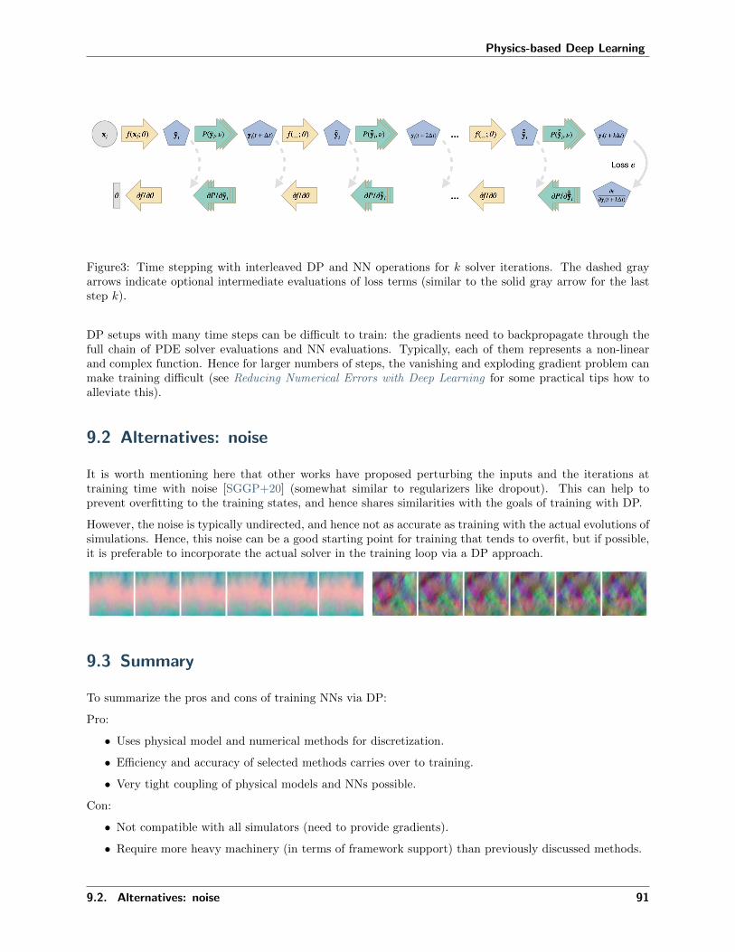
Physics-based Deep Learning
Figure3: Time stepping with interleaved DP and NN operations for 𝑘 solver iterations. The dashed grayarrows indicate optional intermediate evaluations of loss terms (similar to the solid gray arrow for the laststep 𝑘).
DP setups with many time steps can be difficult to train: the gradients need to backpropagate through thefull chain of PDE solver evaluations and NN evaluations. Typically, each of them represents a non-linearand complex function. Hence for larger numbers of steps, the vanishing and exploding gradient problem canmake training difficult (see Reducing Numerical Errors with Deep Learning for some practical tips how toalleviate this).
9.2 Alternatives: noise
It is worth mentioning here that other works have proposed perturbing the inputs and the iterations attraining time with noise [SGGP+20] (somewhat similar to regularizers like dropout). This can help toprevent overfitting to the training states, and hence shares similarities with the goals of training with DP.
However, the noise is typically undirected, and hence not as accurate as training with the actual evolutions ofsimulations. Hence, this noise can be a good starting point for training that tends to overfit, but if possible,it is preferable to incorporate the actual solver in the training loop via a DP approach.
9.3 Summary
To summarize the pros and cons of training NNs via DP:
Pro:
• Uses physical model and numerical methods for discretization.
• Efficiency and accuracy of selected methods carries over to training.
• Very tight coupling of physical models and NNs possible.
Con:
• Not compatible with all simulators (need to provide gradients).
• Require more heavy machinery (in terms of framework support) than previously discussed methods.
9.2. Alternatives: noise 91

Physics-based Deep Learning
Here, the last negative point (regarding heavy machinery) is bound to strongly improve in a fairly shortamount of time. However, for now it’s important to keep in mind that not every simulator is suitable forDP training out of the box. Hence, in this book we’ll focus on examples using phiflow, which was designedfor interfacing with deep learning frameworks.
Next we can target more some complex scenarios to showcase what can be achieved with differentiablephysics. This will also illustrate how the right selection of numerical methods for a DP operator yieldsimprovements in terms of training accuracy.
92 Chapter 9. Discussion
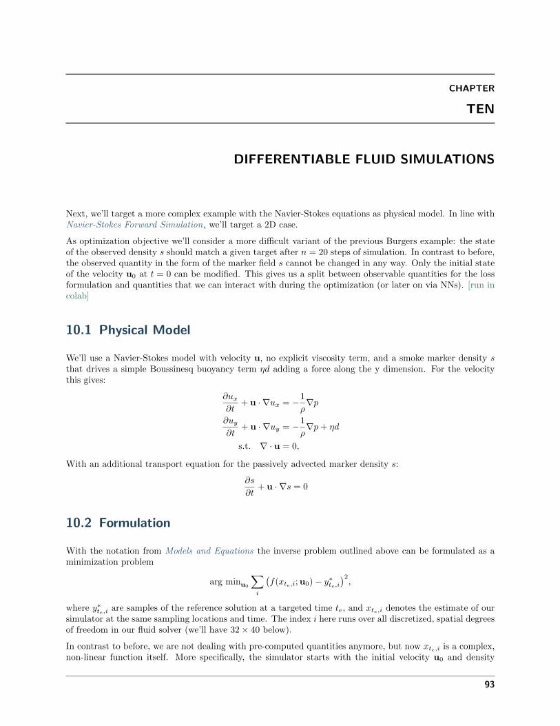
CHAPTER
TEN
DIFFERENTIABLE FLUID SIMULATIONS
Next, we’ll target a more complex example with the Navier-Stokes equations as physical model. In line withNavier-Stokes Forward Simulation, we’ll target a 2D case.
As optimization objective we’ll consider a more difficult variant of the previous Burgers example: the stateof the observed density 𝑠 should match a given target after 𝑛 = 20 steps of simulation. In contrast to before,the observed quantity in the form of the marker field 𝑠 cannot be changed in any way. Only the initial stateof the velocity u0 at 𝑡 = 0 can be modified. This gives us a split between observable quantities for the lossformulation and quantities that we can interact with during the optimization (or later on via NNs). [run incolab]
10.1 Physical Model
We’ll use a Navier-Stokes model with velocity u, no explicit viscosity term, and a smoke marker density 𝑠that drives a simple Boussinesq buoyancy term 𝜂𝑑 adding a force along the y dimension. For the velocitythis gives:
𝜕𝑢𝑥
𝜕𝑡+ u · ∇𝑢𝑥 = −1
𝜌∇𝑝
𝜕𝑢𝑦
𝜕𝑡+ u · ∇𝑢𝑦 = −1
𝜌∇𝑝 + 𝜂𝑑
s.t. ∇ · u = 0,
With an additional transport equation for the passively advected marker density 𝑠:
𝜕𝑠
𝜕𝑡+ u · ∇𝑠 = 0
10.2 Formulation
With the notation from Models and Equations the inverse problem outlined above can be formulated as aminimization problem
arg minu0
∑𝑖
(𝑓(𝑥𝑡𝑒,𝑖;u0) − 𝑦*𝑡𝑒,𝑖
)2,
where 𝑦*𝑡𝑒,𝑖 are samples of the reference solution at a targeted time 𝑡𝑒, and 𝑥𝑡𝑒,𝑖 denotes the estimate of oursimulator at the same sampling locations and time. The index 𝑖 here runs over all discretized, spatial degreesof freedom in our fluid solver (we’ll have 32 × 40 below).
In contrast to before, we are not dealing with pre-computed quantities anymore, but now 𝑥𝑡𝑒,𝑖 is a complex,non-linear function itself. More specifically, the simulator starts with the initial velocity u0 and density
93

Physics-based Deep Learning
𝑠0 to compute the 𝑥𝑡𝑒,𝑖, by 𝑛 evaluations of the discretized PDE 𝒫. This gives as simulated final state𝑦𝑡𝑒,𝑖 = 𝑠𝑡𝑒 = 𝒫𝑛(u0, 𝑠0), where we will leave 𝑠0 fixed in the following, and focus on u0 as our degrees offreedom. Hence, the optimization can only change u0 to align 𝑦𝑡𝑒,𝑖 with the references 𝑦*𝑡𝑒,𝑖 as closely aspossible.
10.3 Starting the Implementation
First, let’s get the loading of python modules out of the way. By importing phi.torch.flow, we get fluidsimulation functions that work within pytorch graphs and can provide gradients (phi.tf.flow would be thealternative for tensorflow).
#!pip install --upgrade --quiet phiflow
!pip install --upgrade --quiet git+https://github.com/tum-pbs/PhiFlow@develop
from phi.torch.flow import *
import pylab # for visualizations later on
10.4 Batched simulations
Now we can set up the simulation, which will work in line with the previous “regular” simulation examplefrom the Navier-Stokes Forward Simulation. However, now we’ll directly include an additional dimension,similar to a mini-batch used for NN training. For this, we’ll introduce a named dimension called inflow loc.This dimension will exist “above” the previous spatial dimensions y, x and the channel dimensions vector.As indicated by the name inflow loc, the main differences for this dimension will lie in different locationsof the inflow, in order to obtain different flow simulations. The named dimensions in phiflow make it veryconvenient to broadcast information across matching dimensions in different tensors.
The Domain object is allocated just like before, but the INFLOW LOCATION tensor now receives a string'inflow loc,vector' that indicates the names of the two dimensions. This leads to the creation of aninflow loc dimensions in addition to the two spatial dimensions (the vector part).
# closed domain
INFLOW_LOCATION = tensor([(12, 4), (13, 6), (14, 5), (16, 5)], batch('inflow_loc'), channel('vector→˓'))INFLOW = (1./3.) * CenteredGrid(Sphere(center=INFLOW_LOCATION, radius=3), extrapolation.BOUNDARY,
→˓x=32, y=40, bounds=Box[0:32, 0:40])
BND = extrapolation.ZERO # closed, boundary conditions for velocity grid below
# uncomment this for a slightly different open domain case
#INFLOW_LOCATION = tensor([(11, 6), (12, 4), (14, 5), (16, 5)], batch('inflow_loc'), channel(
→˓'vector'))#INFLOW = (1./4.) * CenteredGrid(Sphere(center=INFLOW_LOCATION, radius=3), extrapolation.BOUNDARY,
→˓x=32, y=40, bounds=Box[0:32, 0:40])
#BND = extrapolation.BOUNDARY # open boundaries
INFLOW.shape
(inflow_loc=4, x=32, y=40)
94 Chapter 10. Differentiable Fluid Simulations

Physics-based Deep Learning
The last statement verifies that our INFLOW grid likewise has an inflow loc dimension in addition to thespatial dimensions x and y. You can test for the existence of a tensor dimension in phiflow with the .exists
boolean, which can be evaluated for any dimension name. E.g., above INFLOW.inflow loc.exists will giveTrue, while INFLOW.some unknown dim.exists will give False. The 𝑏 superscript indicates that inflow loc
is a batch dimension.
Phiflow tensors are automatically broadcast to new dimensions via their names, and hence typically no-reshaping operations are required. E.g., you can easily add or multiply tensors with differing dimen-sions. Below we’ll multiply a staggered grid with a tensor of ones along the inflow loc dimensionto get a staggered velocity that has x,y,inflow loc as dimensions via StaggeredGrid(...) * math.
ones(batch(inflow loc=4)).
We can easily simulate a few steps now starting with these different initial conditions. Thanks to thebroadcasting, the exact same code we used for the single forward simulation in the overview chapter willproduce four simulations with different smoke inflow positions.
smoke = CenteredGrid(0, extrapolation.BOUNDARY, x=32, y=40, bounds=Box[0:32, 0:40]) # sampled at
→˓cell centers
velocity = StaggeredGrid(0, BND, x=32, y=40, bounds=Box[0:32, 0:40]) # sampled in staggered form
→˓at face centers
def step(smoke, velocity):
smoke = advect.mac_cormack(smoke, velocity, dt=1) + INFLOW
buoyancy_force = smoke * (0, 1) >> velocity
velocity = advect.semi_lagrangian(velocity, velocity, dt=1) + buoyancy_force
velocity, _ = fluid.make_incompressible(velocity)
return smoke, velocity
for _ in range(20):
smoke,velocity = step(smoke,velocity)
# store and show final states (before optimization)
smoke_final = smoke
fig, axes = pylab.subplots(1, 4, figsize=(10, 6))
for i in range(INFLOW.shape.get_size('inflow_loc')):axes[i].imshow(smoke_final.values.numpy('inflow_loc,y,x')[i,...], origin='lower', cmap='magma')axes[i].set_title(f"Inflow INFLOW_LOCATION.numpy('inflow_loc,vector')[i] " + (", Reference" if
→˓i==3 else ""))
pylab.tight_layout()
The last image shows the state of the advected smoke fields after 20 simulation steps. The final smoke shapeof simulation [3] with an inflow at (16,5), with the straight plume on the far right, will be our referencestate below. The initial velocity of the other three will be modified in the optimization procedure below tomatch this reference.
10.4. Batched simulations 95
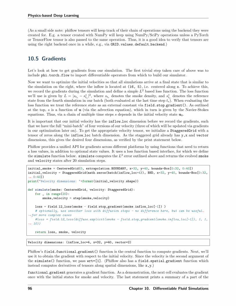
Physics-based Deep Learning
(As a small side note: phiflow tensors will keep track of their chain of operations using the backend they werecreated for. E.g. a tensor created with NumPy will keep using NumPy/SciPy operations unless a PyTorchor TensorFlow tensor is also passed to the same operation. Thus, it is a good idea to verify that tensors areusing the right backend once in a while, e.g., via GRID.values.default backend.)
10.5 Gradients
Let’s look at how to get gradients from our simulation. The first trivial step taken care of above was toinclude phi.torch.flow to import differentiable operators from which to build our simulator.
Now we want to optimize the initial velocities so that all simulations arrive at a final state that is similar tothe simulation on the right, where the inflow is located at (16, 5), i.e. centered along x. To achieve this,we record the gradients during the simulation and define a simple 𝐿2 based loss function. The loss functionwe’ll use is given by 𝐿 = |𝑠𝑡𝑒 − 𝑠*𝑡𝑒 |
2, where 𝑠𝑡𝑒 denotes the smoke density, and 𝑠*𝑡𝑒 denotes the referencestate from the fourth simulation in our batch (both evaluated at the last time step 𝑡𝑒). When evaluating theloss function we treat the reference state as an external constant via field.stop gradient(). As outlinedat the top, 𝑠 is a function of u (via the advection equation), which in turn is given by the Navier-Stokesequations. Thus, via a chain of multiple time steps 𝑠 depends in the initial velocity state u0.
It is important that our initial velocity has the inflow loc dimension before we record the gradients, suchthat we have the full “mini-batch” of four versions of our velocity (three of which will be updated via gradientsin our optimization later on). To get the appropriate velocity tensor, we initialize a StaggeredGrid with atensor of zeros along the inflow loc batch dimension. As the staggered grid already has y,x and vector
dimensions, this gives the desired four dimensions, as verified by the print statement below.
Phiflow provides a unified API for gradients across different platforms by using functions that need to returna loss values, in addition to optional state values. It uses a loss function based interface, for which we definethe simulate function below. simulate computes the 𝐿2 error outlined above and returns the evolved smoke
and velocity states after 20 simulation steps.
initial_smoke = CenteredGrid(0, extrapolation.BOUNDARY, x=32, y=40, bounds=Box[0:32, 0:40])
initial_velocity = StaggeredGrid(math.zeros(batch(inflow_loc=4)), BND, x=32, y=40, bounds=Box[0:32,
→˓ 0:40])
print("Velocity dimensions: "+format(initial_velocity.shape))
def simulate(smoke: CenteredGrid, velocity: StaggeredGrid):
for _ in range(20):
smoke,velocity = step(smoke,velocity)
loss = field.l2_loss(smoke - field.stop_gradient(smoke.inflow_loc[-1]) )
# optionally, use smoother loss with diffusion steps - no difference here, but can be useful
→˓for more complex cases
#loss = field.l2_loss(diffuse.explicit(smoke - field.stop_gradient(smoke.inflow_loc[-1]), 1, 1,
→˓ 10))
return loss, smoke, velocity
Velocity dimensions: (inflow_loc=4, x=32, y=40, vector=2)
Phiflow’s field.functional gradient() function is the central function to compute gradients. Next, we’lluse it to obtain the gradient with respect to the initial velocity. Since the velocity is the second argument ofthe simulate() function, we pass wrt=[1]. (Phiflow also has a field.spatial gradient function whichinstead computes derivatives of tensors along spatial dimensions, like x,y.)
functional gradient generates a gradient function. As a demonstration, the next cell evaluates the gradientonce with the initial states for smoke and velocity. The last statement prints a summary of a part of the
96 Chapter 10. Differentiable Fluid Simulations

Physics-based Deep Learning
resulting gradient tensor.
sim_grad = field.functional_gradient(simulate, wrt=[1], get_output=False)
(velocity_grad,) = sim_grad(initial_smoke, initial_velocity)
print("Some gradient info: " + format(velocity_grad))
print(format(velocity_grad.values.inflow_loc[0].vector[0])) # one example, location 0, x component,
→˓ automatically prints size & content range
Some gradient info: StaggeredGrid[(inflow_loc=4, x=32, y=40, vector=2), size=(32, 40),
→˓extrapolation=0]
(x=31, y=40) float32 -17.366662979125977 < ... < 14.014090538024902
The last two lines just print some information about the resulting gradient field. Naturally, it has the sameshape as the velocity itself: it’s a staggered grid with four inflow locations. The last line shows how to accessthe x-components of one of the gradients.
We could use this to take a look at the content of the computed gradient with regular plotting functions,e.g., by converting the x component of one of the simulations to a numpy array via velocity grad.values.
inflow loc[0].vector[0].numpy('y,x'). However, below we’ll use phiflow’s view() function instead. Itautomatically analyzes the grid content and provides UI buttons to choose different viewing modes. Youcan use them to show arrows, single components of the 2-dimensional velocity vectors, or their magnitudes.(Because of its interactive nature, the corresponding image won’t show up outside of Jupyter, though.)
# neat phiflow helper function:
view(velocity_grad)
Not surprisingly, the fourth gradient on the left is zero (it’s already matching the reference). The other threegradients have detected variations for the initial round inflow positions shown as positive and negative regionsaround the circular shape of the inflow. The ones for the larger distances on the left are also noticeablylarger.
10.6 Optimization
The gradient visualized above is just the linearized change that points in the direction of an increasing loss.Now we can proceed by updating the initial velocities in the opposite direction to minimize the loss, anditerate to find a minimizer.
This is a difficult task: the simulation is producing different dynamics due to the differing initial spatialdensity configuration. Our optimization should now find a single initial velocity state that gives the samestate as the reference simulation at 𝑡 = 20. Thus, after 20 non-linear update steps the simulation shouldreproduce the desired marker density state. It would be much easier to simply change the position of themarker inflow to arrive at this goal, but - to make things more difficult and interesting here - the inflow isnot a degree of freedom. The optimizer can only change the initial velocity u0.
The following cell implements a simple steepest gradient descent optimization: it re-evaluates the gradientfunction, and iterates several times to optimize u0 with a learning rate (step size) LR.
field.functional gradient has a parameter get output that determines whether the original results ofthe function (simulate() in our case) are returned, or only the gradient. As it’s interesting to track howthe loss evolves over the course of the iterations, let’s redefine the gradient function with get output=True.
sim_grad_wloss = field.functional_gradient(simulate, wrt=[1], get_output=True) # if we need
→˓outputs...
(continues on next page)
10.6. Optimization 97

Physics-based Deep Learning
(continued from previous page)
LR = 1e-03
for optim_step in range(80):
(loss, _smoke, _velocity), (velocity_grad,) = sim_grad_wloss(initial_smoke, initial_velocity)
initial_velocity = initial_velocity - LR * velocity_grad
if optim_step<3 or optim_step%10==9: print('Optimization step %d, loss: %f' % (optim_step, np.
→˓sum(loss.numpy()) ))
Optimization step 0, loss: 1193.145020
Optimization step 1, loss: 1165.816650
Optimization step 2, loss: 1104.294556
Optimization step 10, loss: 861.661743
Optimization step 20, loss: 775.154846
Optimization step 30, loss: 747.199829
Optimization step 40, loss: 684.146729
Optimization step 50, loss: 703.087158
Optimization step 60, loss: 660.258423
Optimization step 70, loss: 649.957214
The loss should have gone down significantly, from above 1100 to below 700, and now we can also visualizethe initial velocities that were obtained in the optimization.
The following images show the resulting three initial velocities in terms of their x (first set), and y components(second set of images). We’re skipping the fourth set with inflow loc[0] because it only contains zeros.
fig, axes = pylab.subplots(1, 3, figsize=(10, 4))
for i in range(INFLOW.shape.get_size('inflow_loc')-1):im = axes[i].imshow(initial_velocity.staggered_tensor().numpy('inflow_loc,y,x,vector')[i,...,0],
→˓origin='lower', cmap='magma')axes[i].set_title(f"Ini. vel. X INFLOW_LOCATION.numpy('inflow_loc,vector')[i] ")pylab.colorbar(im,ax=axes[i])
pylab.tight_layout()
fig, axes = pylab.subplots(1, 3, figsize=(10, 4))
for i in range(INFLOW.shape.get_size('inflow_loc')-1):im = axes[i].imshow(initial_velocity.staggered_tensor().numpy('inflow_loc,y,x,vector')[i,...,1],
→˓origin='lower', cmap='magma')axes[i].set_title(f"Ini. vel. Y INFLOW_LOCATION.numpy('inflow_loc,vector')[i] ")pylab.colorbar(im,ax=axes[i])
pylab.tight_layout()
98 Chapter 10. Differentiable Fluid Simulations
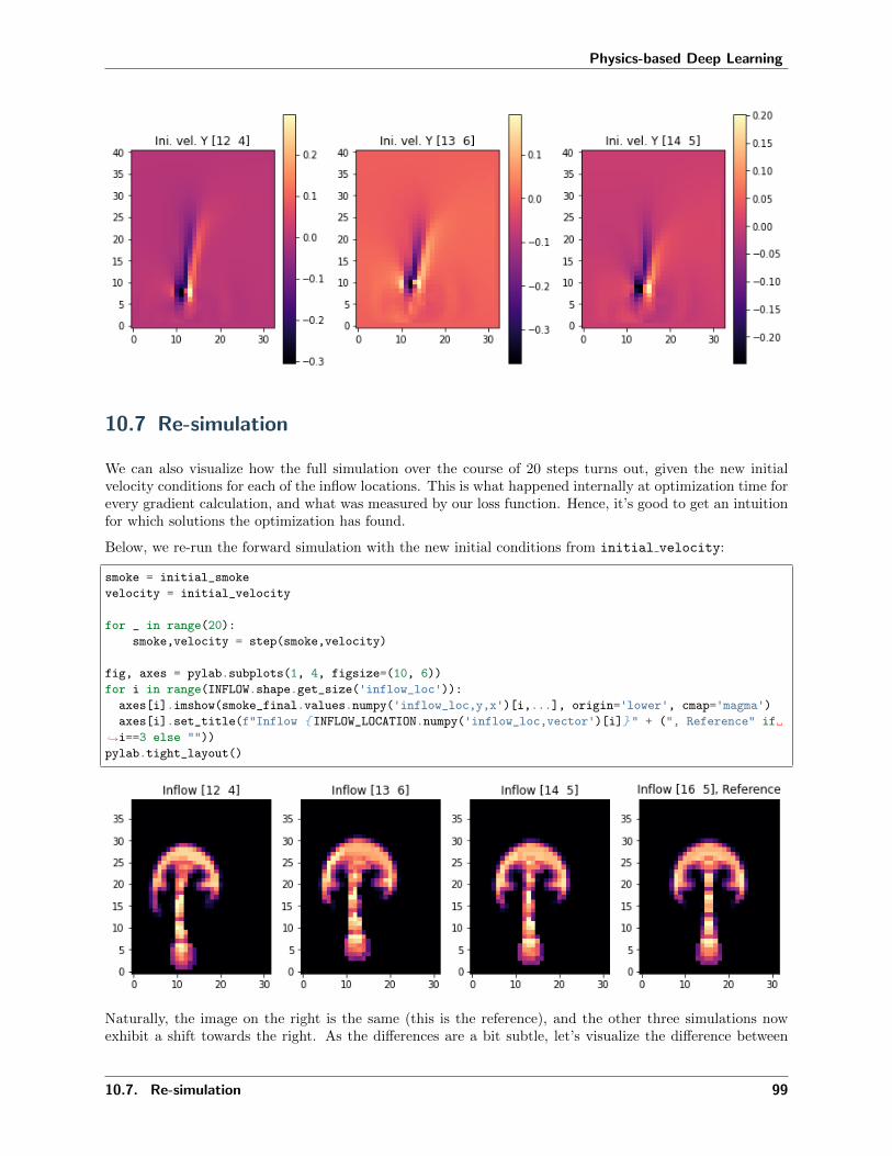
Physics-based Deep Learning
10.7 Re-simulation
We can also visualize how the full simulation over the course of 20 steps turns out, given the new initialvelocity conditions for each of the inflow locations. This is what happened internally at optimization time forevery gradient calculation, and what was measured by our loss function. Hence, it’s good to get an intuitionfor which solutions the optimization has found.
Below, we re-run the forward simulation with the new initial conditions from initial velocity:
smoke = initial_smoke
velocity = initial_velocity
for _ in range(20):
smoke,velocity = step(smoke,velocity)
fig, axes = pylab.subplots(1, 4, figsize=(10, 6))
for i in range(INFLOW.shape.get_size('inflow_loc')):axes[i].imshow(smoke_final.values.numpy('inflow_loc,y,x')[i,...], origin='lower', cmap='magma')axes[i].set_title(f"Inflow INFLOW_LOCATION.numpy('inflow_loc,vector')[i] " + (", Reference" if
→˓i==3 else ""))
pylab.tight_layout()
Naturally, the image on the right is the same (this is the reference), and the other three simulations nowexhibit a shift towards the right. As the differences are a bit subtle, let’s visualize the difference between
10.7. Re-simulation 99

Physics-based Deep Learning
the target configuration and the different final states.
The following images contain the difference between the evolved simulated and target density. Hence, darkregions indicate where the target should be, but isn’t. The top row shows the original states with the initialvelocity being zero, while the bottom row shows the versions after the optimization has tuned the initialvelocities. Hence, in each column you can compare before (top) and after (bottom):
fig, axes = pylab.subplots(2, 3, figsize=(10, 6))
for i in range(INFLOW.shape.get_size('inflow_loc')-1):axes[0,i].imshow(smoke_final.values.numpy('inflow_loc,y,x')[i,...] - smoke_final.values.numpy(
→˓'inflow_loc,y,x')[3,...], origin='lower', cmap='magma')axes[0,i].set_title(f"Org. diff. INFLOW_LOCATION.numpy('inflow_loc,vector')[i] ")pylab.colorbar(im,ax=axes[0,i])
for i in range(INFLOW.shape.get_size('inflow_loc')-1):axes[1,i].imshow(smoke.values.numpy('inflow_loc,y,x')[i,...] - smoke_final.values.numpy('inflow_
→˓loc,y,x')[3,...], origin='lower', cmap='magma')axes[1,i].set_title(f"Result INFLOW_LOCATION.numpy('inflow_loc,vector')[i] ")pylab.colorbar(im,ax=axes[1,i])
These difference images clearly show that the optimization managed to align the upper region of the plumesvery well. Each original image (at the top) shows a clear misalignment in terms of a black halo, whilethe states after optimization largely overlap the target smoke configuration of the reference, and exhibitdifferences closer to zero for the front of each smoke cloud.
Note that all three simulations need to “work” with a fixed inflow, hence they cannot simply “produce”marker density out of the blue to match the target. Also each simulation needs to take into account howthe non-linear model equations change the state of the system over the course of 20 time steps. So theoptimization goal is quite difficult, and it is not possible to exactly satisfy the constraints to match thereference simulation in this scenario. E.g., this is noticeable at the stems of the smoke plumes, which stillshow a black halo after the optimization. The optimization was not able to shift the inflow position, andhence needs to focus on aligning the upper regions of the plumes.
100 Chapter 10. Differentiable Fluid Simulations
Physics-based Deep Learning
10.8 Conclusions
This example illustrated how the differentiable physics approach can easily be extended towards significantlymore complex PDEs. Above, we’ve optimized for a mini-batch of 20 steps of a full Navier-Stokes solver.
This is a powerful basis to bring NNs into the picture. As you might have noticed, our degrees of freedomwere still a regular grid, and we’ve jointly solved a single inverse problem. There were three cases to solveas a mini-batch, of course, but nonetheless the setup still represents a direct optimization. Thus, in linewith the PINN example of Burgers Optimization with a Physics-Informed NN we’ve not really dealt with amachine learning task here. However, that will be the topic of the next chapters.
10.9 Next steps
Based on the code example above, we can recommend experimenting with the following:
• Modify the setup of the simulation to differ more strongly across the four instances, run longer, or usea finer spatial discretization (i.e. larger grid size). Note that this will make the optimization problemtougher, and hence might not converge directly with this simple setup.
• As a larger change, add a multi-resolution optimization to handle cases with larger differences. I.e., firstsolve with a coarse discretization, and then uses this solution as an initial guess for a finer discretization.
10.8. Conclusions 101

Physics-based Deep Learning
102 Chapter 10. Differentiable Fluid Simulations

CHAPTER
ELEVEN
DIFFERENTIABLE PHYSICS VERSUS PHYSICS-INFORMEDTRAINING
In the previous sections we’ve seen example reconstructions that used physical residuals as soft constraints,in the form of the PINNs, and reconstructions that used a differentiable physics (DP) solver. While bothmethods can find minimizers for similar inverse problems, the obtained solutions differ substantially, as doesthe behavior of the non-linear optimization problem that we get from each formulation. In the followingwe discuss these differences in more detail, and we will combine conclusions drawn from the behavior ofthe Burgers case of Burgers Optimization with a Physics-Informed NN and Burgers Optimization with aDifferentiable Physics Gradient with observations from research papers.
11.1 Compatibility with existing numerical methods
It is very obvious that the PINN implementation is quite simple, which is a positive aspect, but at the sametime it differs strongly from “typical” discretizations and solution approaches that are usually employed tosolve PDEs like Burgers equation. The derivatives are computed via the neural network, and hence rely ona fairly accurate representation of the solution to provide a good direction for optimization problems.
The DP version on the other hand inherently relies on a numerical solver that is tied into the learning process.As such it requires a discretization of the problem at hand, and via this discretization can employ existing,and potentially powerful numerical techniques. This means solutions and derivatives can be evaluated withknown and controllable accuracy, and can be evaluated efficiently.
11.2 Discretization
The reliance on a suitable discretization requires some understanding and knowledge of the problem underconsideration. A sub-optimal discretization can impede the learning process or, worst case, lead to divergingtraining runs. However, given the large body of theory and practical realizations of stable solvers for a widevariety of physical problems, this is typically not an unsurmountable obstacle.
The PINN approaches on the other hand do not require an a-priori choice of a discretization, and as suchseems to be “discretization-less”. This, however, is only an advantage on first sight. As they yield solutionsin a computer, they naturally have to discretize the problem, but they construct this discretization over thecourse of the training process, in a way that is not easily controllable from the outside. Thus, the resultingaccuracy is determined by how well the training manages to estimate the complexity of the problem forrealistic use cases, and how well the training data approximates the unknown regions of the solution.
103

Physics-based Deep Learning
As demonstrated with the Burgers example, the PINN solutions typically have significant difficulties propa-gating information backward in time. This is closely coupled to the efficiency of the method.
11.3 Efficiency
The PINN approaches typically perform a localized sampling and correction of the solutions, which means thecorrections in the form of weight updates are likewise typically local. The fulfillment of boundary conditionsin space and time can be correspondingly slow, leading to long training runs in practice.
A well-chosen discretization of a DP approach can remedy this behavior, and provide an improved flow ofgradient information. At the same time, the reliance on a computational grid means that solutions can beobtained very quickly. Given an interpolation scheme or a set of basis functions, the solution can be sampledat any point in space or time given a very local neighborhood of the computational grid. Worst case, thiscan lead to slight memory overheads, e.g., by repeatedly storing mostly constant values of a solution.
For the PINN representation with fully-connected networks on the other hand, we need to make a full passover the potentially large number of values in the whole network to obtain a sample of the solution at asingle point. The network effectively needs to encode the full high-dimensional solution, and its size likewisedetermines the efficiency of derivative calculations.
11.4 Efficiency continued
That being said, because the DP approaches can cover much larger solution manifolds, the structure of thesemanifolds is typically also difficult to learn. E.g., when training a network with a larger number of iterations(i.e. a long look-ahead into the future), this typically represents a signal that is more difficult to learn thana short look ahead.
As a consequence, these training runs not only take more computational resources per NN iteration, theyalso need longer to converge. Regarding resources, each computation of the look-ahead potentially requiresa large number of simulation steps, and typically a similar amount of resources for the backpropagation step.Regarding convergence, the more complex signal that should be learned can take more training iterationsand require larger NN structures.
11.5 Summary
The following table summarizes these pros and cons of physics-informed (PI) and differentiable physics (DP)approaches:
104 Chapter 11. Differentiable Physics versus Physics-informed Training

Physics-based Deep Learning
Method Pro ConPI - Analytic derivatives via backpropaga-
tion.- Expensive evaluation of NN, as well as derivativecalculations.
- Easy to implement. - Incompatible with existing numerical methods.- No control of discretization.
DP - Leverage existing numerical methods. - More complicated implementation.- Efficient evaluation of simulation andderivatives.
- Require understanding of problem to choose suitablediscretization.
As a summary, both methods are definitely interesting, and have a lot of potential. There are numerousmore complicated extensions and algorithmic modifications that change and improve on the various negativeaspects we have discussed for both sides.
However, as of this writing, the physics-informed (PI) approach has clear limitations when it comes toperformance and compatibility with existing numerical methods. Thus, when knowledge of the problem athand is available, which typically is the case when we choose a suitable PDE model to constrain the learningprocess, employing a differentiable physics solver can significantly improve the training process as well as thequality of the obtained solution. Next, we will target more complex settings, i.e., fluids with Navier-Stokes,to illustrate this in more detail.
11.5. Summary 105

Physics-based Deep Learning
106 Chapter 11. Differentiable Physics versus Physics-informed Training
Part IV
Complex Examples with DP
107


CHAPTER
TWELVE
COMPLEX EXAMPLES OVERVIEW
The following sections will give code examples of more complex cases to show what can be achieved viadifferentiable physics training.
First, we’ll show a scenario that employs deep learning to represent the errors of numerical simulations,following Um et al. [UBH+20]. This is a very fundamental task, and requires the learned model to closelyinteract with a numerical solver. Hence, it’s a prime example of situations where it’s crucial to bring thenumerical solver into the deep learning loop.
Next, we’ll show how to let NNs solve tough inverse problems, namely the long-term control of a Navier-Stokes simulation, following Holl et al. [HKT19]. This task requires long term planning, and hence needstwo networks, one to predict the evolution, and another one to act to reach the desired goal. (Later on, inControlling Burgers’ Equation with Reinforcement Learning we will compare this approach to another DLvariant using reinforcement learning.)
Both cases require quite a bit more resources than the previous examples, so you can expect these notebooksto run longer (and it’s a good idea to use check-pointing when working with these examples).
109

Physics-based Deep Learning
110 Chapter 12. Complex Examples Overview

CHAPTER
THIRTEEN
REDUCING NUMERICAL ERRORS WITH DEEP LEARNING
First, we’ll target numerical errors that arise in the discretization of a continuous PDE 𝒫*, i.e. when weformulate 𝒫. This approach will demonstrate that, despite the lack of closed-form descriptions, discretizationerrors often are functions with regular and repeating structures and, thus, can be learned by a neural network.Once the network is trained, it can be evaluated locally to improve the solution of a PDE-solver, i.e., toreduce its numerical error. The resulting method is a hybrid one: it will always run (a coarse) PDE solver,and then improve it at runtime with corrections inferred by an NN.
Pretty much all numerical methods contain some form of iterative process: repeated updates over time forexplicit solvers, or within a single update step for implicit solvers. An example for the second case could befound here, but below we’ll target the first case, i.e. iterations over time. [run in colab]
13.1 Problem formulation
In the context of reducing errors, it’s crucial to have a differentiable physics solver, so that the learningprocess can take the reaction of the solver into account. This interaction is not possible with supervisedlearning or PINN training. Even small inference errors of a supervised NN can accumulate over time, andlead to a data distribution that differs from the distribution of the pre-computed data. This distributionshift can lead to sub-optimal results, or even cause blow-ups of the solver.
In order to learn the error function, we’ll consider two different discretizations of the same PDE 𝒫*: areference version, which we assume to be accurate, with a discretized version 𝒫𝑟, and solutions r ∈ R, whereR denotes the manifold of solutions of 𝒫𝑟. In parallel to this, we have a less accurate approximation of thesame PDE, which we’ll refer to as the source version, as this will be the solver that our NN should later oninteract with. Analogously, we have 𝒫𝑠 with solutions s ∈ S . After training, we’ll obtain a hybrid solverthat uses 𝒫𝑠 in conjunction with a trained network to obtain improved solutions, i.e., solutions that arecloser to the ones produced by 𝒫𝑟.
Figure1: Visual overview of coarse and reference manifolds
111

Physics-based Deep Learning
Let’s assume 𝒫 advances a solution by a time step ∆𝑡, and let’s denote 𝑛 consecutive steps by a superscript:𝒫𝑛𝑠 (𝒯 r𝑡) = 𝒫𝑠(𝒫𝑠(· · · 𝒫𝑠(𝒯 r𝑡) · · · )). The corresponding state of the simulation is s𝑡+𝑛 = 𝒫𝑛(𝒯 r𝑡). Here we
assume a mapping operator 𝒯 exists that transfers a reference solution to the source manifold. This could,e.g., be a simple downsampling operation. Especially for longer sequences, i.e. larger 𝑛, the source states𝑡+𝑛 will deviate from a corresponding reference state r𝑡+𝑛. This is what we will address with an NN in thefollowing.
As before, we’ll use an 𝐿2-norm to quantify the deviations, i.e., an error function 𝑒(s𝑡, 𝒯 r𝑡) = ‖s𝑡−𝒯 r𝑡‖2. Ourlearning goal is to train at a correction operator 𝒞(s) such that a solution to which the correction is appliedhas a lower error than the original unmodified (source) solution: 𝑒(𝒫𝑠(𝒞(𝒯 r𝑡)), 𝒯 r𝑡+1) < 𝑒(𝒫𝑠(𝒯 r𝑡), 𝒯 r𝑡+1).
The correction function 𝒞(s|𝜃) is represented as a deep neural network with weights 𝜃 and receives the states to infer an additive correction field with the same dimension. To distinguish the original states s from thecorrected ones, we’ll denote the latter with an added tilde s. The overall learning goal now becomes
arg min𝜃
((𝒫𝑠𝒞)𝑛(𝒯 r𝑡) − 𝒯 r𝑡+𝑛
)2To simplify the notation, we’ve dropped the sum over different samples here (the 𝑖 from previous versions).A crucial bit that’s easy to overlook in the equation above, is that the correction depends on the modifiedstates, i.e. it is a function of s, so we have 𝒞(s|𝜃). These states actually evolve over time when training.They don’t exist beforehand.
TL;DR: We’ll train a network 𝒞 to reduce the numerical errors of a simulator with a more accurate reference.It’s crucial to have the source solver realized as a differential physics operator, such that it can give gradientsfor an improved training of 𝒞.
13.2 Getting started with the implementation
The following replicates an experiment) from Solver-in-the-loop: learning from differentiable physics tointeract with iterative pde-solvers [HKT19], further details can be found in section B.1 of the appendix ofthe paper.
First, let’s download the prepared data set (for details on generation & loading cf. https://github.com/tum-pbs/Solver-in-the-Loop), and let’s get the data handling out of the way, so that we can focus on theinteresting parts...
import os, sys, logging, argparse, pickle, glob, random, distutils.dir_util, urllib.request
fname_train = 'sol-karman-2d-train.pickle'if not os.path.isfile(fname_train):
print("Downloading training data (73MB), this can take a moment the first time...")
urllib.request.urlretrieve("https://physicsbaseddeeplearning.org/data/"+fname_train, fname_train)
with open(fname_train, 'rb') as f: data_preloaded = pickle.load(f)
print("Loaded data, training sims".format(len(data_preloaded)) )
Downloading training data (73MB), this can take a moment the first time...
Loaded data, 6 training sims
Also let’s get installing / importing all the necessary libraries out of the way. And while we’re at it, we canset the random seed - obviously, 42 is the ultimate choice here
112 Chapter 13. Reducing Numerical Errors with Deep Learning

Physics-based Deep Learning
#!pip install --upgrade --quiet phiflow
#!pip uninstall phiflow
!pip install --upgrade --quiet git+https://github.com/tum-pbs/PhiFlow@develop
from phi.tf.flow import *
import tensorflow as tf
from tensorflow import keras
random.seed(42)
np.random.seed(42)
tf.random.set_seed(42)
13.3 Simulation setup
Now we can set up the source simulation 𝒫𝑠. Note that we won’t deal with 𝒫𝑟 below: the downsampledreference data is contained in the training data set. It was generated with a four times finer discretization.Below we’re focusing on the interaction of the source solver and the NN.
This code block and the next ones will define lots of functions, that will be used later on for training.
The KarmanFlow solver below simulates a relatively standard wake flow case with a spherical obstacle ina rectangular domain, and an explicit viscosity solve to obtain different Reynolds numbers. This is thegeometry of the setup:
Figure2: Domain setup for the wake flow case (sizes in the imlpementation are using an additional factor of100).
The solver applies inflow boundary conditions for the y-velocity with a pre-multiplied mask (vel BcMask),to set the y components at the bottom of the domain during the simulation step. This mask is createdwith the HardGeometryMask from phiflow, which initializes the spatially shifted entries for the componentsof a staggered grid correctly. The simulation step is quite straight forward: it computes contributions forviscosity, inflow, advection and finally makes the resulting motion divergence free via an implicit pressuresolve:
class KarmanFlow():
def __init__(self, domain):
self.domain = domain
(continues on next page)
13.3. Simulation setup 113
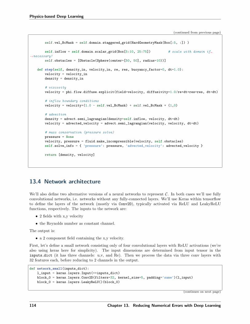
Physics-based Deep Learning
(continued from previous page)
self.vel_BcMask = self.domain.staggered_grid(HardGeometryMask(Box[:5, :]) )
self.inflow = self.domain.scalar_grid(Box[5:10, 25:75]) # scale with domain if
→˓necessary!
self.obstacles = [Obstacle(Sphere(center=[50, 50], radius=10))]
def step(self, density_in, velocity_in, re, res, buoyancy_factor=0, dt=1.0):
velocity = velocity_in
density = density_in
# viscosity
velocity = phi.flow.diffuse.explicit(field=velocity, diffusivity=1.0/re*dt*res*res, dt=dt)
# inflow boundary conditions
velocity = velocity*(1.0 - self.vel_BcMask) + self.vel_BcMask * (1,0)
# advection
density = advect.semi_lagrangian(density+self.inflow, velocity, dt=dt)
velocity = advected_velocity = advect.semi_lagrangian(velocity, velocity, dt=dt)
# mass conservation (pressure solve)
pressure = None
velocity, pressure = fluid.make_incompressible(velocity, self.obstacles)
self.solve_info = 'pressure': pressure, 'advected_velocity': advected_velocity
return [density, velocity]
13.4 Network architecture
We’ll also define two alternative versions of a neural networks to represent 𝒞. In both cases we’ll use fullyconvolutional networks, i.e. networks without any fully-connected layers. We’ll use Keras within tensorflowto define the layers of the network (mostly via Conv2D), typically activated via ReLU and LeakyReLUfunctions, respectively. The inputs to the network are:
• 2 fields with x,y velocity
• the Reynolds number as constant channel.
The output is:
• a 2 component field containing the x,y velocity.
First, let’s define a small network consisting only of four convolutional layers with ReLU activations (we’realso using keras here for simplicity). The input dimensions are determined from input tensor in theinputs dict (it has three channels: u,v, and Re). Then we process the data via three conv layers with32 features each, before reducing to 2 channels in the output.
def network_small(inputs_dict):
l_input = keras.layers.Input(**inputs_dict)
block_0 = keras.layers.Conv2D(filters=32, kernel_size=5, padding='same')(l_input)block_0 = keras.layers.LeakyReLU()(block_0)
(continues on next page)
114 Chapter 13. Reducing Numerical Errors with Deep Learning
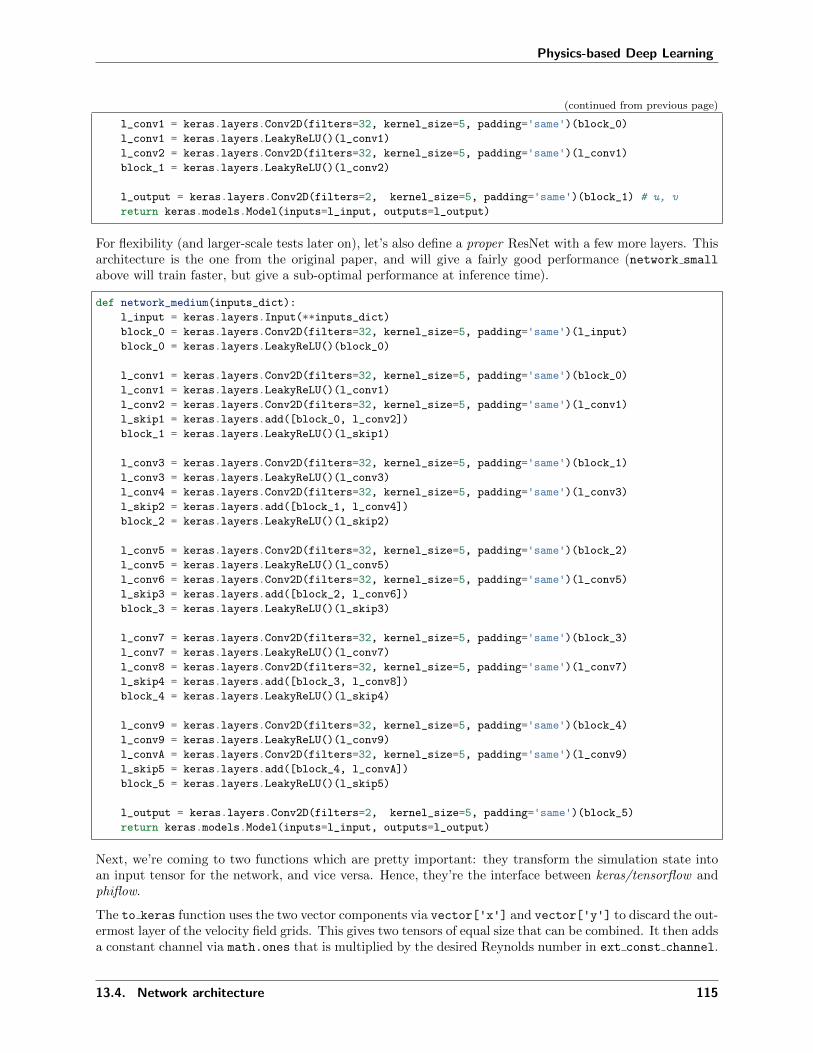
Physics-based Deep Learning
(continued from previous page)
l_conv1 = keras.layers.Conv2D(filters=32, kernel_size=5, padding='same')(block_0)l_conv1 = keras.layers.LeakyReLU()(l_conv1)
l_conv2 = keras.layers.Conv2D(filters=32, kernel_size=5, padding='same')(l_conv1)block_1 = keras.layers.LeakyReLU()(l_conv2)
l_output = keras.layers.Conv2D(filters=2, kernel_size=5, padding='same')(block_1) # u, v
return keras.models.Model(inputs=l_input, outputs=l_output)
For flexibility (and larger-scale tests later on), let’s also define a proper ResNet with a few more layers. Thisarchitecture is the one from the original paper, and will give a fairly good performance (network small
above will train faster, but give a sub-optimal performance at inference time).
def network_medium(inputs_dict):
l_input = keras.layers.Input(**inputs_dict)
block_0 = keras.layers.Conv2D(filters=32, kernel_size=5, padding='same')(l_input)block_0 = keras.layers.LeakyReLU()(block_0)
l_conv1 = keras.layers.Conv2D(filters=32, kernel_size=5, padding='same')(block_0)l_conv1 = keras.layers.LeakyReLU()(l_conv1)
l_conv2 = keras.layers.Conv2D(filters=32, kernel_size=5, padding='same')(l_conv1)l_skip1 = keras.layers.add([block_0, l_conv2])
block_1 = keras.layers.LeakyReLU()(l_skip1)
l_conv3 = keras.layers.Conv2D(filters=32, kernel_size=5, padding='same')(block_1)l_conv3 = keras.layers.LeakyReLU()(l_conv3)
l_conv4 = keras.layers.Conv2D(filters=32, kernel_size=5, padding='same')(l_conv3)l_skip2 = keras.layers.add([block_1, l_conv4])
block_2 = keras.layers.LeakyReLU()(l_skip2)
l_conv5 = keras.layers.Conv2D(filters=32, kernel_size=5, padding='same')(block_2)l_conv5 = keras.layers.LeakyReLU()(l_conv5)
l_conv6 = keras.layers.Conv2D(filters=32, kernel_size=5, padding='same')(l_conv5)l_skip3 = keras.layers.add([block_2, l_conv6])
block_3 = keras.layers.LeakyReLU()(l_skip3)
l_conv7 = keras.layers.Conv2D(filters=32, kernel_size=5, padding='same')(block_3)l_conv7 = keras.layers.LeakyReLU()(l_conv7)
l_conv8 = keras.layers.Conv2D(filters=32, kernel_size=5, padding='same')(l_conv7)l_skip4 = keras.layers.add([block_3, l_conv8])
block_4 = keras.layers.LeakyReLU()(l_skip4)
l_conv9 = keras.layers.Conv2D(filters=32, kernel_size=5, padding='same')(block_4)l_conv9 = keras.layers.LeakyReLU()(l_conv9)
l_convA = keras.layers.Conv2D(filters=32, kernel_size=5, padding='same')(l_conv9)l_skip5 = keras.layers.add([block_4, l_convA])
block_5 = keras.layers.LeakyReLU()(l_skip5)
l_output = keras.layers.Conv2D(filters=2, kernel_size=5, padding='same')(block_5)return keras.models.Model(inputs=l_input, outputs=l_output)
Next, we’re coming to two functions which are pretty important: they transform the simulation state intoan input tensor for the network, and vice versa. Hence, they’re the interface between keras/tensorflow andphiflow.
The to keras function uses the two vector components via vector['x'] and vector['y'] to discard the out-ermost layer of the velocity field grids. This gives two tensors of equal size that can be combined. It then addsa constant channel via math.ones that is multiplied by the desired Reynolds number in ext const channel.
13.4. Network architecture 115

Physics-based Deep Learning
The resulting stack of grids is stacked along the channels dimensions, and represents an input to the neuralnetwork.
After network evaluation, we transform the output tensor back into a phiflow grid via the to phiflow
function. It converts the 2-component tensor that is returned by the network into a phiflow staggered gridobject, so that it is compatible with the velocity field of the fluid simulation. (Note: these are two centeredgrids with different sizes, so we leave the work to the domain.staggered grid function, which also setsphysical size and boundary conditions as given by the domain object).
def to_keras(dens_vel_grid_array, ext_const_channel):
# align the sides the staggered velocity grid making its size the same as the centered grid
return math.stack(
[
math.pad( dens_vel_grid_array[1].vector['x'].values, 'x':(0,1) , math.extrapolation.
→˓ZERO),
dens_vel_grid_array[1].vector['y'].y[:-1].values, # v
math.ones(dens_vel_grid_array[0].shape)*ext_const_channel # Re
],
math.channel('channels'))
def to_phiflow(tf_tensor, domain):
return domain.staggered_grid(
math.stack(
[
math.tensor(tf.pad(tf_tensor[..., 1], [(0,0), (0,1), (0,0)]), math.batch('batch'),→˓math.spatial('y, x')), # v
math.tensor( tf_tensor[...,:-1, 0], math.batch('batch'), math.spatial('y, x')), #
→˓u
], math.channel('vector'))
)
13.5 Data handling
So far so good - we also need to take care of a few more mundane tasks, e.g., some data handling andrandomization. Below we define a Dataset class that stores all “ground truth” reference data (alreadydownsampled).
We actually have a lot of data dimensions: multiple simulations, with many time steps, each with differentfields. This makes the code below a bit more difficult to read.
The data format for the numpy array dataPreloaded: is ['sim name', frame, field (dens & vel)],where each field has dimension [batch-size, y-size, x-size, channels] (this is the standard for aphiflow export).
class Dataset():
def __init__(self, data_preloaded, num_frames, num_sims=None, batch_size=1, is_testset=False):
self.epoch = None
self.epochIdx = 0
self.batch = None
self.batchIdx = 0
self.step = None
self.stepIdx = 0
(continues on next page)
116 Chapter 13. Reducing Numerical Errors with Deep Learning

Physics-based Deep Learning
(continued from previous page)
self.dataPreloaded = data_preloaded
self.batchSize = batch_size
self.numSims = num_sims
self.numBatches = num_sims//batch_size
self.numFrames = num_frames
self.numSteps = num_frames
# initialize directory keys (using naming scheme from SoL codebase)
# constant additional per-sim channel: Reynolds numbers from data generation
# hard coded for training and test data here
if not is_testset:
self.dataSims = ['karman-fdt-hires-set/sim_%06d '%i for i in range(num_sims) ]
ReNrs = [160000.0, 320000.0, 640000.0, 1280000.0, 2560000.0, 5120000.0]
self.extConstChannelPerSim = self.dataSims[i]:[ReNrs[i]] for i in range(num_sims)
else:
self.dataSims = ['karman-fdt-hires-testset/sim_%06d '%i for i in range(num_sims) ]
ReNrs = [120000.0, 480000.0, 1920000.0, 7680000.0]
self.extConstChannelPerSim = self.dataSims[i]:[ReNrs[i]] for i in range(num_sims)
self.dataFrames = [ np.arange(num_frames) for _ in self.dataSims ]
# debugging example, check shape of a single marker density field:
#print(format(self.dataPreloaded[self.dataSims[0]][0][0].shape ))
# the data has the following shape ['sim', frame, field (dens/vel)] where each field is
→˓[batch-size, y-size, x-size, channels]
self.resolution = self.dataPreloaded[self.dataSims[0]][0][0].shape[1:3]
# compute data statistics for normalization
self.dataStats =
'std': (
np.std(np.concatenate([np.absolute(self.dataPreloaded[asim][i][0].reshape(-1)) for
→˓asim in self.dataSims for i in range(num_frames)], axis=-1)), # density
np.std(np.concatenate([np.absolute(self.dataPreloaded[asim][i][1].reshape(-1)) for
→˓asim in self.dataSims for i in range(num_frames)], axis=-1)), # x-velocity
np.std(np.concatenate([np.absolute(self.dataPreloaded[asim][i][2].reshape(-1)) for
→˓asim in self.dataSims for i in range(num_frames)], axis=-1)), # y-velocity
)
self.dataStats.update(
'ext.std': [ np.std([np.absolute(self.extConstChannelPerSim[asim][0]) for asim in self.
→˓dataSims]) ] # Reynolds Nr
)
if not is_testset:
print("Data stats: "+format(self.dataStats))
# re-shuffle data for next epoch
def newEpoch(self, exclude_tail=0, shuffle_data=True):
self.numSteps = self.numFrames - exclude_tail
simSteps = [ (asim, self.dataFrames[i][0:(len(self.dataFrames[i])-exclude_tail)]) for i,
→˓asim in enumerate(self.dataSims) ]
(continues on next page)
13.5. Data handling 117

Physics-based Deep Learning
(continued from previous page)
sim_step_pair = []
for i,_ in enumerate(simSteps):
sim_step_pair += [ (i, astep) for astep in simSteps[i][1] ] # (sim_idx, step) ...
if shuffle_data: random.shuffle(sim_step_pair)
self.epoch = [ list(sim_step_pair[i*self.numSteps:(i+1)*self.numSteps]) for i in
→˓range(self.batchSize*self.numBatches) ]
self.epochIdx += 1
self.batchIdx = 0
self.stepIdx = 0
def nextBatch(self):
self.batchIdx += self.batchSize
self.stepIdx = 0
def nextStep(self):
self.stepIdx += 1
The nextEpoch, nextBatch, and nextStep functions will be called at training time to randomize the orderof the training data.
Now we need one more function that compiles the data for a mini batch to train with, called getData below.It returns batches of the desired size in terms of marker density, velocity, and Reynolds number.
# for class Dataset():
def getData(self, consecutive_frames):
d_hi = [
np.concatenate([
self.dataPreloaded[
self.dataSims[self.epoch[self.batchIdx+i][self.stepIdx][0]] # sim_key
][
self.epoch[self.batchIdx+i][self.stepIdx][1]+j # frames
][0]
for i in range(self.batchSize)
], axis=0) for j in range(consecutive_frames+1)
]
u_hi = [
np.concatenate([
self.dataPreloaded[
self.dataSims[self.epoch[self.batchIdx+i][self.stepIdx][0]] # sim_key
][
self.epoch[self.batchIdx+i][self.stepIdx][1]+j # frames
][1]
for i in range(self.batchSize)
], axis=0) for j in range(consecutive_frames+1)
]
v_hi = [
np.concatenate([
self.dataPreloaded[
self.dataSims[self.epoch[self.batchIdx+i][self.stepIdx][0]] # sim_key
][
self.epoch[self.batchIdx+i][self.stepIdx][1]+j # frames
][2]
for i in range(self.batchSize)
], axis=0) for j in range(consecutive_frames+1)
]
ext = [(continues on next page)
118 Chapter 13. Reducing Numerical Errors with Deep Learning

Physics-based Deep Learning
(continued from previous page)
self.extConstChannelPerSim[
self.dataSims[self.epoch[self.batchIdx+i][self.stepIdx][0]]
][0] for i in range(self.batchSize)
]
return [d_hi, u_hi, v_hi, ext]
Note that the density here denotes a passively advected marker field, and not the density of the fluid. Belowwe’ll be focusing on the velocity only, the marker density is tracked purely for visualization purposes.
After all the definitions we can finally run some code. We can define the dataset object with the downloadeddata from the first cell.
nsims = 6
batch_size = 3
simsteps = 500
dataset = Dataset( data_preloaded=data_preloaded, num_frames=simsteps, num_sims=nsims, batch_
→˓size=batch_size )
Data stats: 'std': (2.6542656, 0.23155601, 0.3066732), 'ext.std': [1732512.6262166172]
Additionally, we’ve defined several global variables to control the training and the simulation in the nextcode cells.
The most important and interesting one is msteps. It defines the number of simulation steps that areunrolled at each training iteration. This directly influences the runtime of each training step, as we firsthave to simulate all steps forward, and then backpropagate the gradient through all msteps simulation stepsinterleaved with the NN evaluations. However, this is where we’ll receive important feedback in terms ofgradients how the inferred corrections actually influence a running simulation. Hence, larger msteps aretypically better.
In addition we define the resolution of the simulation in source res, and allocate the fluid solver objectcalled simulator. In order to create grids, it requires access to a Domain object, which mostly exists forconvenience purposes: it stores resolution, physical size in bounds, and boundary conditions of the domain.This information needs to be passed to every grid, and hence it’s convenient to have it in one place in theform of the Domain. For the setup described above, we need different boundary conditions along x and y:closed walls, and free flow in and out of the domain, respecitvely.
We also instantiate the actual NN network in the next cell.
# one of the most crucial! how many simulation steps to look into the future while training
msteps = 4
# # this is the actual resolution in terms of cells
source_res = list(dataset.resolution)
# # this is a virtual size, in terms of abstract units for the bounding box of the domain (it's→˓important for conversions or when rescaling to physical units)
simulation_length = 100.
# for readability
from phi.physics._boundaries import Domain, OPEN, STICKY as CLOSED
boundary_conditions =
'x':(phi.physics._boundaries.STICKY,phi.physics._boundaries.STICKY),'y':(phi.physics._boundaries.OPEN, phi.physics._boundaries.OPEN)
(continues on next page)
13.5. Data handling 119
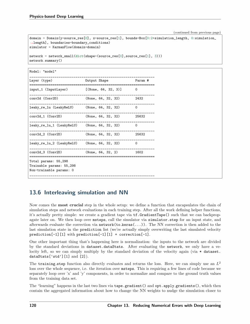
Physics-based Deep Learning
(continued from previous page)
domain = Domain(y=source_res[0], x=source_res[1], bounds=Box[0:2*simulation_length, 0:simulation_
→˓length], boundaries=boundary_conditions)
simulator = KarmanFlow(domain=domain)
network = network_small(dict(shape=(source_res[0],source_res[1], 3)))
network.summary()
Model: "model"
_________________________________________________________________
Layer (type) Output Shape Param #
=================================================================
input_1 (InputLayer) [(None, 64, 32, 3)] 0
_________________________________________________________________
conv2d (Conv2D) (None, 64, 32, 32) 2432
_________________________________________________________________
leaky_re_lu (LeakyReLU) (None, 64, 32, 32) 0
_________________________________________________________________
conv2d_1 (Conv2D) (None, 64, 32, 32) 25632
_________________________________________________________________
leaky_re_lu_1 (LeakyReLU) (None, 64, 32, 32) 0
_________________________________________________________________
conv2d_2 (Conv2D) (None, 64, 32, 32) 25632
_________________________________________________________________
leaky_re_lu_2 (LeakyReLU) (None, 64, 32, 32) 0
_________________________________________________________________
conv2d_3 (Conv2D) (None, 64, 32, 2) 1602
=================================================================
Total params: 55,298
Trainable params: 55,298
Non-trainable params: 0
_________________________________________________________________
13.6 Interleaving simulation and NN
Now comes the most crucial step in the whole setup: we define a function that encapsulates the chain ofsimulation steps and network evaluations in each training step. After all the work defining helper functions,it’s actually pretty simple: we create a gradient tape via tf.GradientTape() such that we can backprop-agate later on. We then loop over msteps, call the simulator via simulator.step for an input state, andafterwards evaluate the correction via network(to keras(...)). The NN correction is then added to thelast simulation state in the prediction list (we’re actually simply overwriting the last simulated velocityprediction[-1][1] with prediction[-1][1] + correction[-1].
One other important thing that’s happening here is normalization: the inputs to the network are dividedby the standard deviations in dataset.dataStats. After evaluating the network, we only have a ve-locity left, so we can simply multiply by the standard deviation of the velocity again (via * dataset.
dataStats['std'][1] and [2]).
The training step function also directly evaluates and returns the loss. Here, we can simply use an 𝐿2
loss over the whole sequence, i.e. the iteration over msteps. This is requiring a few lines of code because weseparately loop over ’x’ and ’y’ components, in order to normalize and compare to the ground truth valuesfrom the training data set.
The “learning” happens in the last two lines via tape.gradient() and opt.apply gradients(), which thencontain the aggregated information about how to change the NN weights to nudge the simulation closer to
120 Chapter 13. Reducing Numerical Errors with Deep Learning

Physics-based Deep Learning
the reference for the full chain of simulation steps.
def training_step(dens_gt, vel_gt, Re, i_step):
with tf.GradientTape() as tape:
prediction, correction = [ [dens_gt[0],vel_gt[0]] ], [0] # predicted states with
→˓correction, inferred velocity corrections
for i in range(msteps):
prediction += [
simulator.step(
density_in=prediction[-1][0],
velocity_in=prediction[-1][1],
re=Re, res=source_res[1],
)
] # prediction: [[density1, velocity1], [density2, velocity2], ...]
model_input = to_keras(prediction[-1], Re)
model_input /= math.tensor([dataset.dataStats['std'][1], dataset.dataStats['std'][2],→˓dataset.dataStats['ext.std'][0]], channel('channels')) # [u, v, Re]
model_out = network(model_input.native(['batch', 'y', 'x', 'channels']), training=True)
model_out *= [dataset.dataStats['std'][1], dataset.dataStats['std'][2]] # [u, v]
correction += [ to_phiflow(model_out, domain) ] # [velocity_
→˓correction1, velocity_correction2, ...]
prediction[-1][1] = prediction[-1][1] + correction[-1]
#prediction[-1][1] = correction[-1]
# evaluate loss
loss_steps_x = [
tf.nn.l2_loss(
(
vel_gt[i].vector['x'].values.native(('batch', 'y', 'x'))- prediction[i][1].vector['x'].values.native(('batch', 'y', 'x'))
)/dataset.dataStats['std'][1])
for i in range(1,msteps+1)
]
loss_steps_x_sum = tf.math.reduce_sum(loss_steps_x)
loss_steps_y = [
tf.nn.l2_loss(
(
vel_gt[i].vector['y'].values.native(('batch', 'y', 'x'))- prediction[i][1].vector['y'].values.native(('batch', 'y', 'x'))
)/dataset.dataStats['std'][2])
for i in range(1,msteps+1)
]
loss_steps_y_sum = tf.math.reduce_sum(loss_steps_y)
loss = (loss_steps_x_sum + loss_steps_y_sum)/msteps
gradients = tape.gradient(loss, network.trainable_variables)
opt.apply_gradients(zip(gradients, network.trainable_variables))
return math.tensor(loss)
Once defined, we can prepare this function for executing the training step by calling phiflow’s math.
jit compile() function. It automatically maps to the correct pre-compilation step of the chosen backend.
13.6. Interleaving simulation and NN 121

Physics-based Deep Learning
E.g., for TF this internally creates a computational graph, and optimizes the chain of operations. For JAX,it can even compile optimized GPU code (if JAX is set up correctly). Using the jit compilation can make ahuge difference in terms of runtime.
training_step_jit = math.jit_compile(training_step)
13.7 Training
For the training, we use a standard Adam optimizer, and run 15 epochs by default. This should be increasedfor the larger network or to obtain more accurate results. For longer training runs, it would also be beneficialto decrease the learning rate over the course of the epochs, but for simplicity, we’ll keep LR constant here.
Optionally, this is also the right point to load a network state to resume training.
LR = 1e-4
EPOCHS = 15
opt = tf.keras.optimizers.Adam(learning_rate=LR)
# optional, load existing network...
# set to epoch nr. to load existing network from there
resume = 0
if resume>0:
ld_network = keras.models.load_model('./nn_epoch:04d .h5'.format(resume))#ld_network = keras.models.load_model('./nn_final.h5') # or the last one
network.set_weights(ld_network.get_weights())
Finally, we can start training the NN! This is very straight forward now, we simply loop over the desirednumber of iterations, get a batch each time via getData, feed it into the source simulation input source in,and compare it in the loss with the reference data for the batch.
The setup above will automatically take care that the differentiable physics solver used here provides theright gradient information, and provides it to the tensorflow network. Be warned: due to the complexity ofthe setup, this training run can take a while... (If you have a saved nn final.h5 network from a previousrun, you can potentially skip this block and load the previously trained model instead via the cell above.)
steps = 0
for j in range(EPOCHS): # training
dataset.newEpoch(exclude_tail=msteps)
if j<resume:
print('resume: skipping epoch'.format(j+1))steps += dataset.numSteps*dataset.numBatches
continue
for ib in range(dataset.numBatches):
for i in range(dataset.numSteps):
# batch: [[dens0, dens1, ...], [x-velo0, x-velo1, ...], [y-velo0, y-velo1, ...],
→˓[ReynoldsNr(s)]]
batch = getData(dataset, consecutive_frames=msteps)
dens_gt = [ # [density0:CenteredGrid, density1, ...]
domain.scalar_grid(
math.tensor(batch[0][k], math.batch('batch'), math.spatial('y, x'))(continues on next page)
122 Chapter 13. Reducing Numerical Errors with Deep Learning

Physics-based Deep Learning
(continued from previous page)
) for k in range(msteps+1)
]
vel_gt = [ # [velocity0:StaggeredGrid, velocity1, ...]
domain.staggered_grid(
math.stack(
[
math.tensor(batch[2][k], math.batch('batch'), math.spatial('y, x')),math.tensor(batch[1][k], math.batch('batch'), math.spatial('y, x')),
], math.channel('vector'))
) for k in range(msteps+1)
]
re_nr = math.tensor(batch[3], math.batch('batch'))
loss = training_step_jit(dens_gt, vel_gt, re_nr, math.tensor(steps))
steps += 1
if (j==0 and ib==0 and i<3) or (j==0 and ib==0 and i%128==0) or (j>0 and ib==0 and
→˓i==400): # reduce output
print('epoch :03d /:03d , batch :03d /:03d , step :04d /:04d : loss= '.→˓format( j+1, EPOCHS, ib+1, dataset.numBatches, i+1, dataset.numSteps, loss ))
dataset.nextStep()
dataset.nextBatch()
if j%10==9: network.save('./nn_epoch:04d.h5'.format(j+1))
# all done! save final version
network.save('./nn_final.h5'); print("Training done, saved NN")
epoch 001/015, batch 001/002, step 0001/0496: loss=2605.340576171875
epoch 001/015, batch 001/002, step 0002/0496: loss=1485.1646728515625
epoch 001/015, batch 001/002, step 0003/0496: loss=790.8267211914062
epoch 001/015, batch 001/002, step 0129/0496: loss=98.64994049072266
epoch 001/015, batch 001/002, step 0257/0496: loss=75.3546142578125
epoch 001/015, batch 001/002, step 0385/0496: loss=70.05519104003906
epoch 002/015, batch 001/002, step 0401/0496: loss=19.126527786254883
epoch 003/015, batch 001/002, step 0401/0496: loss=9.628664016723633
epoch 004/015, batch 001/002, step 0401/0496: loss=7.898053169250488
epoch 005/015, batch 001/002, step 0401/0496: loss=3.6936004161834717
epoch 006/015, batch 001/002, step 0401/0496: loss=3.172729730606079
epoch 007/015, batch 001/002, step 0401/0496: loss=2.8511123657226562
epoch 008/015, batch 001/002, step 0401/0496: loss=3.4968295097351074
epoch 009/015, batch 001/002, step 0401/0496: loss=1.6942076683044434
epoch 010/015, batch 001/002, step 0401/0496: loss=1.6551270484924316
epoch 011/015, batch 001/002, step 0401/0496: loss=1.9383186101913452
epoch 012/015, batch 001/002, step 0401/0496: loss=2.0140795707702637
epoch 013/015, batch 001/002, step 0401/0496: loss=1.4174892902374268
epoch 014/015, batch 001/002, step 0401/0496: loss=1.2593278884887695
epoch 015/015, batch 001/002, step 0401/0496: loss=1.250532627105713
Training done, saved NN
The loss should go down from above 1000 initially to below 10. This is a good sign, but of course it’s even
13.7. Training 123
Physics-based Deep Learning
more important to see how the NN-solver combination fares on new inputs. With this training approachwe’ve realized a hybrid solver, consisting of a regular source simulator, and a network that was trained tospecifically interact with this simulator for a chosen domain of simulation cases.
Let’s see how well this works by applying it to a set of test data inputs with new Reynolds numbers thatwere not part of the training data.
To keep things somewhat simple, we won’t aim for a high-performance version of our hybrid solver. Forperformance, please check out the external code base: the network trained here should be directly useablein this apply script.
13.8 Evaluation
In order to evaluate the performance of our DL-powered solver, we essentially only need to repeat the innerloop of each training iteration for more steps. While we were limited to msteps evaluations at training time,we can now run our solver for arbitrary lengths. This is a good test for how well our solver has learned tokeep the data within the desired distribution, and represents a generalization test for longer rollouts.
We can reuse the solver code from above, but in the following, we will consider two simulated versions: forcomparison, we’ll run one reference simulation in the source space (i.e., without any modifications). Thisversion receives the regular outputs of each evaluation of the simulator, and ignores the learned correction(stored in steps source below). The second version, repeatedly computes the source solver plus the learnedcorrection, and advances this state in the solver (steps hybrid).
We also need a set of new data. Below, we’ll download a new set of Reynolds numbers (in between the onesused for training), so that we can later on run the unmodified simulator and the DL-powered one on thesecases.
fname_test = 'sol-karman-2d-test.pickle'if not os.path.isfile(fname_test):
print("Downloading test data (38MB), this can take a moment the first time...")
urllib.request.urlretrieve("https://physicsbaseddeeplearning.org/data/"+fname_test, fname_test)
with open(fname_test, 'rb') as f: data_test_preloaded = pickle.load(f)
print("Loaded test data, training sims".format(len(data_test_preloaded)) )
Downloading test data (38MB), this can take a moment the first time...
Loaded test data, 4 training sims
Next we create a new dataset object dataset test that organizes the data. We’re simply using the firstbatch of the unshuffled dataset, though.
A subtle but important point: we still have to use the normalization from the original training data set:dataset.dataStats['std'] values. The test data set has it’s own mean and standard deviation, and sothe trained NN never saw this data before. The NN was trained with the data in dataset above, and hencewe have to use the constants from there for normalization to make sure the network receives values that itcan relate to the data it was trained with.
dataset_test = Dataset( data_preloaded=data_test_preloaded, is_testset=True, num_frames=simsteps,
→˓num_sims=4, batch_size=4 )
# we only need 1 batch with t=0 states to initialize the test simulations with
dataset_test.newEpoch(shuffle_data=False)
batch = getData(dataset_test, consecutive_frames=0)
(continues on next page)
124 Chapter 13. Reducing Numerical Errors with Deep Learning

Physics-based Deep Learning
(continued from previous page)
re_nr_test = math.tensor(batch[3], math.batch('batch')) # Reynolds numbers
print("Reynolds numbers in test data set: "+format(re_nr_test))
Reynolds numbers in test data set: (120000.0, 480000.0, 1920000.0, 7680000.0) along batch
Next we construct a math.tensor as initial state for the centered marker fields, and a staggered grid fromthe next two indices of the test set batch. Similar to to phiflow above, we can use phi.math.stack() tocombine two fields of appropriate size as a staggered grid.
source_dens_initial = math.tensor( batch[0][0], math.batch('batch'), math.spatial('y, x'))
source_vel_initial = domain.staggered_grid(phi.math.stack([
math.tensor(batch[2][0], math.batch('batch'),math.spatial('y, x')),math.tensor(batch[1][0], math.batch('batch'),math.spatial('y, x'))], channel('vector')))
Now we can first run the source simulation for 120 steps as baseline:
source_dens_test, source_vel_test = source_dens_initial, source_vel_initial
steps_source = [[source_dens_test,source_vel_test]]
# note - math.jit_compile() not useful for numpy solve... hence not necessary
for i in range(120):
[source_dens_test,source_vel_test] = simulator.step(
density_in=source_dens_test,
velocity_in=source_vel_test,
re=re_nr_test,
res=source_res[1],
)
steps_source.append( [source_dens_test,source_vel_test] )
print("Source simulation steps "+format(len(steps_source)))
Source simulation steps 121
Next, we compute the corresponding states of our learned hybrid solver. Here, we closely follow the trainingcode, however, now without any gradient tapes or loss computations. We only evaluate the NN in a forwardpass for each simulated state to compute a correction field:
source_dens_test, source_vel_test = source_dens_initial, source_vel_initial
steps_hybrid = [[source_dens_test,source_vel_test]]
for i in range(120):
[source_dens_test,source_vel_test] = simulator.step(
density_in=source_dens_test,
velocity_in=source_vel_test,
re=math.tensor(re_nr_test),
res=source_res[1],
)
model_input = to_keras([source_dens_test,source_vel_test], re_nr_test )
model_input /= math.tensor([dataset.dataStats['std'][1], dataset.dataStats['std'][2], dataset.
→˓dataStats['ext.std'][0]], channel('channels')) # [u, v, Re]
model_out = network(model_input.native(['batch', 'y', 'x', 'channels']), training=False)
model_out *= [dataset.dataStats['std'][1], dataset.dataStats['std'][2]] # [u, v]
correction = to_phiflow(model_out, domain)
(continues on next page)
13.8. Evaluation 125
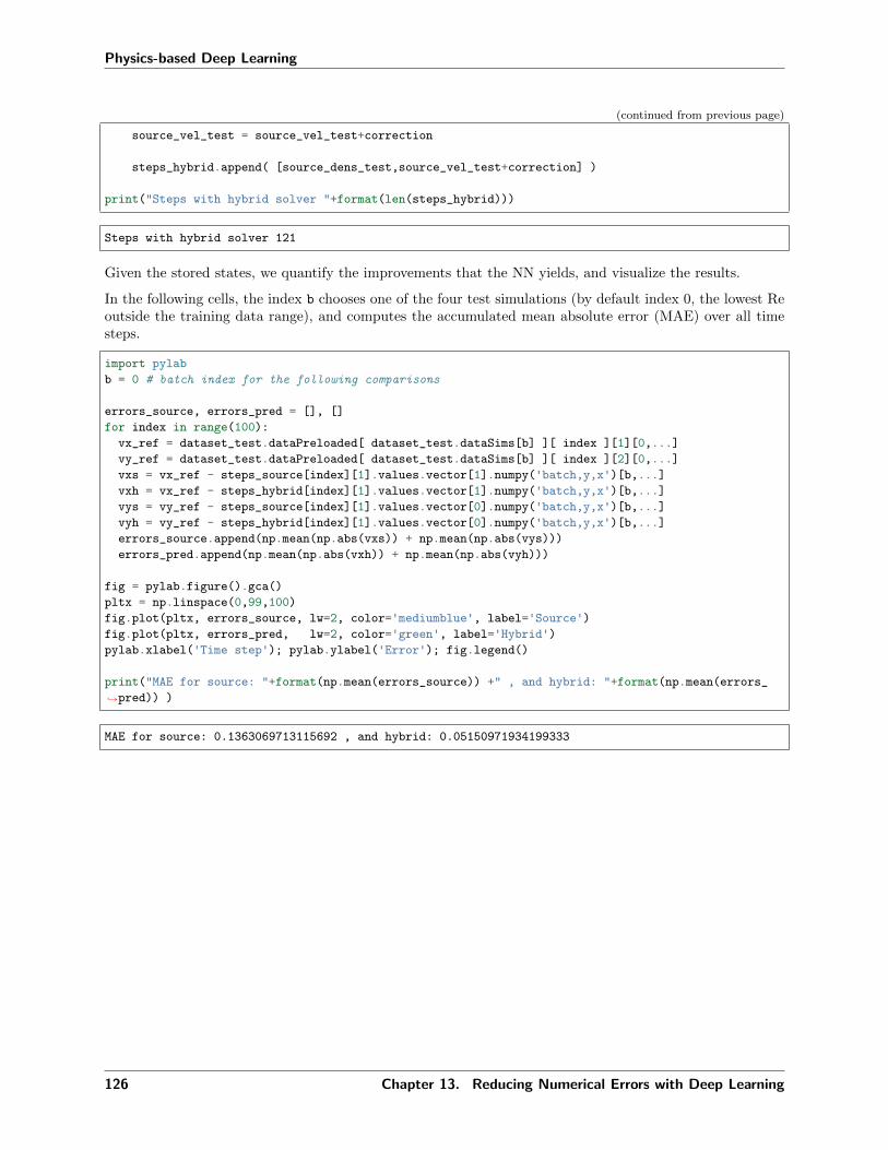
Physics-based Deep Learning
(continued from previous page)
source_vel_test = source_vel_test+correction
steps_hybrid.append( [source_dens_test,source_vel_test+correction] )
print("Steps with hybrid solver "+format(len(steps_hybrid)))
Steps with hybrid solver 121
Given the stored states, we quantify the improvements that the NN yields, and visualize the results.
In the following cells, the index b chooses one of the four test simulations (by default index 0, the lowest Reoutside the training data range), and computes the accumulated mean absolute error (MAE) over all timesteps.
import pylab
b = 0 # batch index for the following comparisons
errors_source, errors_pred = [], []
for index in range(100):
vx_ref = dataset_test.dataPreloaded[ dataset_test.dataSims[b] ][ index ][1][0,...]
vy_ref = dataset_test.dataPreloaded[ dataset_test.dataSims[b] ][ index ][2][0,...]
vxs = vx_ref - steps_source[index][1].values.vector[1].numpy('batch,y,x')[b,...]vxh = vx_ref - steps_hybrid[index][1].values.vector[1].numpy('batch,y,x')[b,...]vys = vy_ref - steps_source[index][1].values.vector[0].numpy('batch,y,x')[b,...]vyh = vy_ref - steps_hybrid[index][1].values.vector[0].numpy('batch,y,x')[b,...]errors_source.append(np.mean(np.abs(vxs)) + np.mean(np.abs(vys)))
errors_pred.append(np.mean(np.abs(vxh)) + np.mean(np.abs(vyh)))
fig = pylab.figure().gca()
pltx = np.linspace(0,99,100)
fig.plot(pltx, errors_source, lw=2, color='mediumblue', label='Source')fig.plot(pltx, errors_pred, lw=2, color='green', label='Hybrid')pylab.xlabel('Time step'); pylab.ylabel('Error'); fig.legend()
print("MAE for source: "+format(np.mean(errors_source)) +" , and hybrid: "+format(np.mean(errors_
→˓pred)) )
MAE for source: 0.1363069713115692 , and hybrid: 0.05150971934199333
126 Chapter 13. Reducing Numerical Errors with Deep Learning

Physics-based Deep Learning
Due to the complexity of the training, the performance can vary, but typically the overall MAE is ca. 160%larger for the regular simulation compared to the hybrid simulator. The gap is typically even bigger for otherReynolds numbers within the training data range. The graph above also shows this behavior over time.
Let’s also visualize the differences of the two outputs by plotting the y component of the velocities over time.The two following code cells show six velocity snapshots for the batch index b in intervals of 20 time steps.
c = 0 # channel selector, x=1 or y=0
interval = 20 # time interval
fig, axes = pylab.subplots(1, 6, figsize=(16, 5))
for i in range(0,6):
v = steps_source[i*interval][1].values.vector[c].numpy('batch,y,x')[b,...]axes[i].imshow( v , origin='lower', cmap='magma')axes[i].set_title(f" Source simulation t= i*interval ")
pylab.tight_layout()
fig, axes = pylab.subplots(1, 6, figsize=(16, 5))
(continues on next page)
13.8. Evaluation 127
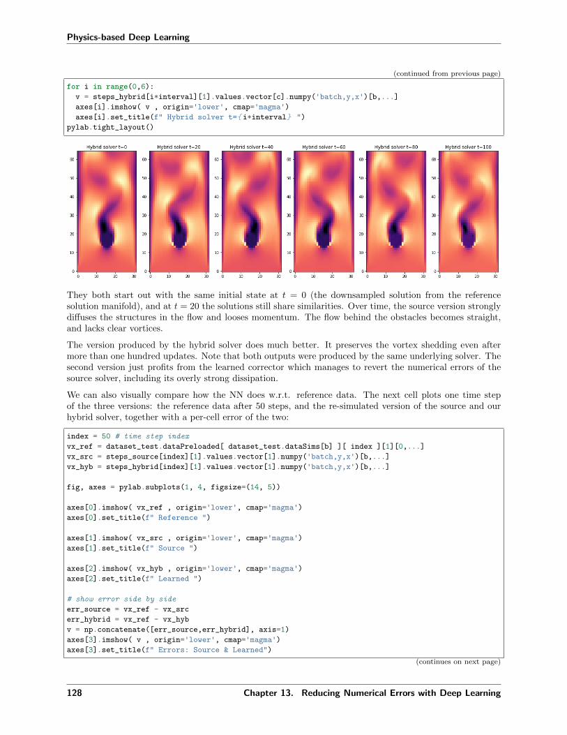
Physics-based Deep Learning
(continued from previous page)
for i in range(0,6):
v = steps_hybrid[i*interval][1].values.vector[c].numpy('batch,y,x')[b,...]axes[i].imshow( v , origin='lower', cmap='magma')axes[i].set_title(f" Hybrid solver t= i*interval ")
pylab.tight_layout()
They both start out with the same initial state at 𝑡 = 0 (the downsampled solution from the referencesolution manifold), and at 𝑡 = 20 the solutions still share similarities. Over time, the source version stronglydiffuses the structures in the flow and looses momentum. The flow behind the obstacles becomes straight,and lacks clear vortices.
The version produced by the hybrid solver does much better. It preserves the vortex shedding even aftermore than one hundred updates. Note that both outputs were produced by the same underlying solver. Thesecond version just profits from the learned corrector which manages to revert the numerical errors of thesource solver, including its overly strong dissipation.
We can also visually compare how the NN does w.r.t. reference data. The next cell plots one time stepof the three versions: the reference data after 50 steps, and the re-simulated version of the source and ourhybrid solver, together with a per-cell error of the two:
index = 50 # time step index
vx_ref = dataset_test.dataPreloaded[ dataset_test.dataSims[b] ][ index ][1][0,...]
vx_src = steps_source[index][1].values.vector[1].numpy('batch,y,x')[b,...]vx_hyb = steps_hybrid[index][1].values.vector[1].numpy('batch,y,x')[b,...]
fig, axes = pylab.subplots(1, 4, figsize=(14, 5))
axes[0].imshow( vx_ref , origin='lower', cmap='magma')axes[0].set_title(f" Reference ")
axes[1].imshow( vx_src , origin='lower', cmap='magma')axes[1].set_title(f" Source ")
axes[2].imshow( vx_hyb , origin='lower', cmap='magma')axes[2].set_title(f" Learned ")
# show error side by side
err_source = vx_ref - vx_src
err_hybrid = vx_ref - vx_hyb
v = np.concatenate([err_source,err_hybrid], axis=1)
axes[3].imshow( v , origin='lower', cmap='magma')axes[3].set_title(f" Errors: Source & Learned")
(continues on next page)
128 Chapter 13. Reducing Numerical Errors with Deep Learning

Physics-based Deep Learning
(continued from previous page)
pylab.tight_layout()
This shows very clearly how the pure source simulation in the middle deviates from the reference on the left.The learned version stays much closer to the reference solution.
The two per-cell error images on the right also illustrate this: the source version has much larger errors (i.e.brighter colors) that show how it systematically underestimates the vortices that should form. The error forthe learned version is much more evenly distributed and significantly smaller in magnitude.
This concludes our evaluation. Note that the improved behavior of the hybrid solver can be difficult toreliably measure with simple vector norms such as an MAE or 𝐿2 norm. To improve this, we’d need toemploy other, domain-specific metrics. In this case, metrics for fluids based on vorticity and turbulenceproperties of the flow would be applicable. However, in this text, we instead want to focus on DL-relatedtopics and target another inverse problem with differentiable physics solvers in the next chapter.
13.9 Next steps
• Modify the training to further reduce the training error. With the medium network you should be ableto get the loss down to around 1.
• Turn off the differentiable physics training (by setting msteps=1), and compare it with the DP version.
• Likewise, train a network with a larger msteps setting, e.g., 8 or 16. Note that due to the recurrentnature of the training, you’ll probably have to load a pre-trained state to stabilize the first iterations.
• Use the external github code to generate new test data, and run your trained NN on these cases. You’llsee that a reduced training error not always directly correlates with an improved test performance.
13.9. Next steps 129

Physics-based Deep Learning
130 Chapter 13. Reducing Numerical Errors with Deep Learning

CHAPTER
FOURTEEN
SOLVING INVERSE PROBLEMS WITH NNS
Inverse problems encompass a large class of practical applications in science. In general, the goal here is notto directly compute a physical field like the velocity at a future time (this is the typical scenario for a forwardsolve), but instead more generically compute one or more parameters in the model equations such that certainconstraints are fulfilled. A very common objective is to find the optimal setting for a single parameter givensome constraints. E.g., this could be the global diffusion constant for an advection-diffusion model such thatit fits measured data as accurately as possible. Inverse problems are encountered for any model parameteradjusted via observations, or the reconstruction of initial conditions, e.g., for particle imaging velocimetry(PIV). More complex cases aim for computing boundary geometries w.r.t. optimal conditions, e.g. to obtaina shape with minimal drag in a fluid flow.
A key aspect below will be that we’re not aiming for solving only a single instance of an inverse problem,but we’d like to use deep learning to solve a larger collection of inverse problems. Thus, unlike the physics-informed example of Burgers Optimization with a Physics-Informed NN or the differentiable physics (DP)optimization of Differentiable Fluid Simulations, where we’ve solved an optimization problem for specificinstances of inverse problems, we now aim for training an NN that learns to solve a larger class of inverseproblems, i.e., a whole solution manifold. Nonetheless, we of course need to rely on a certain degree ofsimilarity for these problems, otherwise there’s nothing to learn (and the implied assumption of continuityin the solution manifold breaks down).
Below we will run a very challenging test case as a representative of these inverse problems: we will aim forcomputing a high dimensional control function that exerts forces over the full course of an incompressiblefluid simulation in order to reach a desired goal state for a passively advected marker in the fluid. Thismeans we only have very indirect constraints to be fulfilled (a single state at the end of a sequence), and alarge number of degrees of freedom (the control force function is a space-time function with the same degreesof freedom as the flow field itself).
The long-term nature of the control is one of the aspects which makes this a tough inverse problem: anychanges to the state of the physical system can lead to large change later on in time, and hence a controllerneeds to anticipate how the system will behave when it is influenced. This means an NN also needs to learnhow the underlying physics evolve and change, and this is exactly where the gradients from the DP trainingcome in to guide the learning task towards solution that can reach the goal. [run in colab]
131

Physics-based Deep Learning
14.1 Formulation
With the notation from Models and Equations this gives the minimization problem
arg min𝜃
∑𝑚
∑𝑖
(𝑓(𝑥𝑚,𝑖; 𝜃) − 𝑦*𝑚,𝑖)2,
where 𝑦*𝑚,𝑖 denotes the samples of the target state of the marker field, and 𝑥𝑚,𝑖 denotes the simulated stateof the marker density. As before, the index 𝑖 samples our solution at different spatial locations (typically allgrid cells), while the index 𝑚 here indicates a large collection of different target states.
Our goal is to train two networks OP and CFE with weights 𝜃OP and 𝜃CFE such that a sequence
u𝑛, 𝑑𝑛 = 𝒫(CFE( 𝒫(CFE(· · · 𝒫(CFE(u0, 𝑑0, 𝑑𝑂𝑃 )) · · · )))) = (𝒫 CFE)𝑛(u0, 𝑑0, 𝑑𝑂𝑃 ).
minimizes the loss above. The OP network is a predictor that determines the state 𝑑𝑂𝑃 that the action ofthe CFE should aim for, i.e., it does the longer term planning from which to determine the action. Giventhe target 𝑑*, it computes 𝑑𝑂𝑃 = OP(𝑑, 𝑑*) = 𝑓OP(𝑑, 𝑑*; 𝜃OP). The CFE acts additively on the velocityfield by computing u + 𝑓CFE(u, 𝑑, 𝑓OP(𝑑, 𝑑*; 𝜃OP); 𝜃CFE), where we’ve used 𝑓OP and 𝑓CFE to denote the NNrepresentations of OP and CFE, respectively, and 𝑑* to denote the target density state. 𝜃OP and 𝜃CFE denotethe corresponding network weights.
For this problem, the model PDE 𝒫 contains a discretized version of the incompressible Navier-Stokesequations in two dimensions for a velocity u:
𝜕𝑢𝑥
𝜕𝑡+ u · ∇𝑢𝑥 = −1
𝜌∇𝑝
𝜕𝑢𝑦
𝜕𝑡+ u · ∇𝑢𝑦 = −1
𝜌∇𝑝
s.t. ∇ · u = 0,
without explicit viscosity, and with an additional transport equation for the marker density 𝑑 given by𝜕𝑑𝜕𝑡 + u · ∇𝑑 = 0.
To summarize, we have a predictor OP that gives us a direction, an actor CFE that exerts a force on aphysical model 𝒫. They all need to play hand in hand to reach a given target after 𝑛 iterations of thesimulation. As apparent from this formulation, it’s not a simple inverse problem, especially due to thefact that all three functions are non-linear. This is exactly why the gradients from the DP approach areso important. (The viewpoint above also indicates that reinforcement learning is a potential option. InControlling Burgers’ Equation with Reinforcement Learning we’ll compare DP with these alternatives.)
14.2 Control of incompressible fluids
The next sections will walk you through all the necessary steps from data generation to network trainingusing 𝜑Flow. Due to the complexity of the control problem, we’ll start with a supervised initialization ofthe networks, before switching to a more accurate end-to-end training with DP. (Note: this example uses anolder version 1.4.1 of 𝜑Flow.)
The code below replicates an inverse problem example (the shape transitions experiment) from Learning toControl PDEs with Differentiable Physics [HKT19], further details can be found in section D.2 of the paper’sappendix.
First we need to load phiflow and check out the PDE-Control git repository, which also contains some numpyarrays with initial shapes.
132 Chapter 14. Solving Inverse Problems with NNs
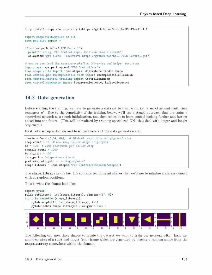
Physics-based Deep Learning
!pip install --upgrade --quiet git+https://github.com/tum-pbs/[email protected]
import matplotlib.pyplot as plt
from phi.flow import *
if not os.path.isdir('PDE-Control'):print("Cloning, PDE-Control repo, this can take a moment")
os.system("git clone --recursive https://github.com/holl-/PDE-Control.git")
# now we can load the necessary phiflow libraries and helper functions
import sys; sys.path.append('PDE-Control/src')from shape_utils import load_shapes, distribute_random_shape
from control.pde.incompressible_flow import IncompressibleFluidPDE
from control.control_training import ControlTraining
from control.sequences import StaggeredSequence, RefinedSequence
14.3 Data generation
Before starting the training, we have to generate a data set to train with, i.e., a set of ground truth timesequences 𝑢*. Due to the complexity of the training below, we’ll use a staged approach that pre-trains asupervised network as a rough initialization, and then refines it to learn control looking further and furtherahead into the future. (This will be realized by training specialized NNs that deal with longer and longersequences.)
First, let’s set up a domain and basic parameters of the data generation step.
domain = Domain([64, 64]) # 1D Grid resolution and physical size
step_count = 16 # how many solver steps to perform
dt = 1.0 # Time increment per solver step
example_count = 1000
batch_size = 100
data_path = 'shape-transitions'pretrain_data_path = 'moving-squares'shape_library = load_shapes('PDE-Control/notebooks/shapes')
The shape library in the last line contains ten different shapes that we’ll use to intialize a marker densitywith at random positions.
This is what the shapes look like:
import pylab
pylab.subplots(1, len(shape_library), figsize=(17, 5))
for t in range(len(shape_library)):
pylab.subplot(1, len(shape_library), t+1)
pylab.imshow(shape_library[t], origin='lower')
The following cell uses these shapes to create the dataset we want to train our network with. Each ex-ample consists of a start and target (end) frame which are generated by placing a random shape from theshape library somewhere within the domain.
14.3. Data generation 133

Physics-based Deep Learning
for scene in Scene.list(data_path): scene.remove()
for _ in range(example_count // batch_size):
scene = Scene.create(data_path, count=batch_size, copy_calling_script=False)
print(scene)
start = distribute_random_shape(domain.resolution, batch_size, shape_library)
end__ = distribute_random_shape(domain.resolution, batch_size, shape_library)
[scene.write_sim_frame([start], ['density'], frame=f) for f in range(step_count)]
scene.write_sim_frame([end__], ['density'], frame=step_count)
shape-transitions/sim_000000
shape-transitions/sim_000100
shape-transitions/sim_000200
shape-transitions/sim_000300
shape-transitions/sim_000400
shape-transitions/sim_000500
shape-transitions/sim_000600
shape-transitions/sim_000700
shape-transitions/sim_000800
shape-transitions/sim_000900
Since this dataset does not contain any intermediate frames, it does not allow for supervised pretraining.This is because to pre-train a CFE network, two consecutive frames are required while to pretrain an OP𝑛
network, three frames with a distance of 𝑛/2 are needed.
Instead, we create a second dataset which contains these intermediate frames. This does not need to be veryclose to the actual dataset since it’s only used for network initialization via pretraining. Here, we linearlymove a rectangle around the domain.
for scene in Scene.list(pretrain_data_path): scene.remove()
for scene_index in range(example_count // batch_size):
scene = Scene.create(pretrain_data_path, count=batch_size, copy_calling_script=False)
print(scene)
pos0 = np.random.randint(10, 56, (batch_size, 2)) # start position
pose = np.random.randint(10, 56, (batch_size, 2)) # end position
size = np.random.randint(6, 10, (batch_size, 2))
for frame in range(step_count+1):
time = frame / float(step_count + 1)
pos = np.round(pos0 * (1 - time) + pose * time).astype(np.int)
density = AABox(lower=pos-size//2, upper=pos-size//2+size).value_at(domain.center_points())
scene.write_sim_frame([density], ['density'], frame=frame)
moving-squares/sim_000000
moving-squares/sim_000100
moving-squares/sim_000200
moving-squares/sim_000300
moving-squares/sim_000400
moving-squares/sim_000500
moving-squares/sim_000600
moving-squares/sim_000700
moving-squares/sim_000800
moving-squares/sim_000900
134 Chapter 14. Solving Inverse Problems with NNs

Physics-based Deep Learning
14.4 Supervised initialization
First we define a split of the 1000 data samples into 100 test, 100 validation, and 800 training samples.
test_range = range(100)
val_range = range(100, 200)
train_range = range(200, 1000)
The following cell trains all OP𝑛 ∀𝑛 ∈ 2, 4, 8, 16. Here the 𝑛 indicates the number of time steps for whichthe network predicts the target. In order to cover longer time horizons, we’re using factors of two here tohierarchically divide the time intervals during which the physical system should be controlled.
The ControlTraining class is used to set up the corresponding optimization problem. The loss for thesupervised initialization is defined as the observation loss in terms of velocity at the center frame:
𝐿sup𝑜 =
OP
(𝑑𝑡𝑖 , 𝑑𝑡𝑗
)− 𝑑*(𝑡𝑖+𝑡𝑗)/2
2.
Consequently, no sequence needs to be simulated (sequence class=None) and an observation loss isrequired at frame 𝑛
2 (obs loss frames=[n // 2]). The pretrained network checkpoints are stored insupervised checkpoints.
Note: The next cell will run for some time. The PDE-Control git repo comes with a set of pre-trainednetworks. So if you want to focus on the evaluation, you can skip the training and load the pretrainednetworks instead by commenting out the training cells, and uncommenting the cells for loading below.
supervised_checkpoints =
for n in [2, 4, 8, 16]:
app = ControlTraining(n, IncompressibleFluidPDE(domain, dt),
datapath=pretrain_data_path, val_range=val_range, train_range=train_
→˓range, trace_to_channel=lambda _: 'density',obs_loss_frames=[n//2], trainable_networks=['OP%d ' % n],
sequence_class=None).prepare()
for i in range(1000):
app.progress() # Run Optimization for one batch
supervised_checkpoints['OP%d ' % n] = app.save_model()
supervised_checkpoints # this is where the checkpoints end up when re-training:
'OP16': '/root/phi/model/control-training/sim_000003/checkpoint_00001000','OP2': '/root/phi/model/control-training/sim_000000/checkpoint_00001000','OP4': '/root/phi/model/control-training/sim_000001/checkpoint_00001000','OP8': '/root/phi/model/control-training/sim_000002/checkpoint_00001000'
# supervised_checkpoints = 'OP%d' % n: 'PDE-Control/networks/shapes/supervised/OP%d_1000' % n for
→˓n in [2, 4, 8, 16]
This concludes the pretraining of the OP networks. These networks make it possible to at least perform arough planning of the motions, which will be refined via end-to-end training below. However, beforehandwe’ll initialize the CFE networks such that we can perform actions, i.e., apply forces to the simulation. Thisis completely decoupled from the OP networks.
14.4. Supervised initialization 135

Physics-based Deep Learning
14.5 CFE pretraining with differentiable physics
To pretrain the CFE networks, we set up a simulation with a single step of the differentiable solver.
The following cell trains the CFE network from scratch. If you have a pretrained network at hand, you canskip the training and load the checkpoint by running the cell after.
app = ControlTraining(1, IncompressibleFluidPDE(domain, dt),
datapath=pretrain_data_path, val_range=val_range, train_range=train_range,
→˓trace_to_channel=lambda _: 'density',obs_loss_frames=[1], trainable_networks=['CFE']).prepare()
for i in range(1000):
app.progress() # Run Optimization for one batch
supervised_checkpoints['CFE'] = app.save_model()
# supervised_checkpoints['CFE'] = 'PDE-Control/networks/shapes/CFE/CFE_2000'
Note that we have not actually set up a simulation for the training, as the CFE network only infers forcesbetween pairs of states.
# [TODO, show preview of CFE only?]
14.6 End-to-end training with differentiable physics
Now that first versions of both network types exist, we can initiate the most important step of the setupat hand: the coupled end-to-end training of both networks via the differentiable fluid solver. While thepretraining stages relied on supervised training, the next step will yield a significantly improved quality forthe control.
To initiate an end-to-end training of the CFE and all OP𝑛 networks with the differentiable physics loss inphiflow, we create a new ControlTraining instance with the staggered execution scheme.
The following cell builds the computational graph with step count solver steps without initializing thenetwork weights.
staggered_app = ControlTraining(step_count, IncompressibleFluidPDE(domain, dt),
datapath=data_path, val_range=val_range, train_range=train_range,
→˓trace_to_channel=lambda _: 'density',obs_loss_frames=[step_count], trainable_networks=['CFE', 'OP2',
→˓'OP4', 'OP8', 'OP16'],sequence_class=StaggeredSequence, learning_rate=5e-4).prepare()
App created. Scene directory is /root/phi/model/control-training/sim_000005 (INFO), 2021-04-09
→˓00:41:17,299n
Sequence class: <class 'control.sequences.StaggeredSequence'> (INFO), 2021-04-09 00:41:17,305n
Partition length 16 sequence (from 0 to 16) at frame 8
Partition length 8 sequence (from 0 to 8) at frame 4
Partition length 4 sequence (from 0 to 4) at frame 2
Partition length 2 sequence (from 0 to 2) at frame 1
Execute -> 1
Execute -> 2
Partition length 2 sequence (from 2 to 4) at frame 3
(continues on next page)
136 Chapter 14. Solving Inverse Problems with NNs

Physics-based Deep Learning
(continued from previous page)
Execute -> 3
Execute -> 4
Partition length 4 sequence (from 4 to 8) at frame 6
Partition length 2 sequence (from 4 to 6) at frame 5
Execute -> 5
Execute -> 6
Partition length 2 sequence (from 6 to 8) at frame 7
Execute -> 7
Execute -> 8
Partition length 8 sequence (from 8 to 16) at frame 12
Partition length 4 sequence (from 8 to 12) at frame 10
Partition length 2 sequence (from 8 to 10) at frame 9
Execute -> 9
Execute -> 10
Partition length 2 sequence (from 10 to 12) at frame 11
Execute -> 11
Execute -> 12
Partition length 4 sequence (from 12 to 16) at frame 14
Partition length 2 sequence (from 12 to 14) at frame 13
Execute -> 13
Execute -> 14
Partition length 2 sequence (from 14 to 16) at frame 15
Execute -> 15
Execute -> 16
Target loss: Tensor("truediv_16:0", shape=(), dtype=float32) (INFO), 2021-04-09 00:41:44,654n
Force loss: Tensor("truediv_107:0", shape=(), dtype=float32) (INFO), 2021-04-09 00:41:51,312n
Supervised loss at frame 16: Tensor("truediv_108:0", shape=(), dtype=float32) (INFO), 2021-04-09
→˓00:41:51,332n
Setting up loss (INFO), 2021-04-09 00:41:51,338n
Preparing data (INFO), 2021-04-09 00:42:32,417n
Initializing variables (INFO), 2021-04-09 00:42:32,443n
Model variables contain 0 total parameters. (INFO), 2021-04-09 00:42:36,418n
Validation (000000): Learning_Rate: 0.0005, GT_obs_16: 399498.75, Loss_reg_unscaled: 1.2424506,
→˓Loss_reg_scale: 1.0, Loss: 798997.5 (INFO), 2021-04-09 00:42:59,618n
The next cell initializes the networks using the supervised checkpoints and then trains all networks jointly.You can increase the number of optimization steps or execute the next cell multiple times to further increaseperformance.
Note: The next cell will run for some time. Optionally, you can skip this cell and load the pretrained networksinstead with code in the cell below.
staggered_app.load_checkpoints(supervised_checkpoints)
for i in range(1000):
staggered_app.progress() # run staggered Optimization for one batch
staggered_checkpoint = staggered_app.save_model()
# staggered_checkpoint = net: 'PDE-Control/networks/shapes/staggered/all_53750' for net in ['CFE',→˓ 'OP2', 'OP4', 'OP8', 'OP16']# staggered_app.load_checkpoints(staggered_checkpoint)
14.6. End-to-end training with differentiable physics 137

Physics-based Deep Learning
Now that the network is trained, we can infer some trajectories from the test set. (This corresponds to Fig5b and 18b of the original paper.)
The following cell takes the first one hundred configurations, i.e. our test set as defined by test range, andlet’s the network infer solutions for the corresponding inverse problems.
states = staggered_app.infer_all_frames(test_range)
Via the index list batches below, you can choose to display some of the solutions. Each row shows a temporalsequence starting with the initial condition, and evolving the simulation with the NN control forces for 16time steps. The last step, at 𝑡 = 16 should match the target shown in the image on the far right.
batches = [0,1,2]
pylab.subplots(len(batches), 10, sharey='row', sharex='col', figsize=(14, 6))
pylab.tight_layout(w_pad=0)
# solutions
for i, batch in enumerate(batches):
for t in range(9):
pylab.subplot(len(batches), 10, t + 1 + i * 10)
pylab.title('t=%d ' % (t * 2))
pylab.imshow(states[t * 2].density.data[batch, ..., 0], origin='lower')
# add targets
testset = BatchReader(Dataset.load(staggered_app.data_path,test_range), staggered_app._channel_
→˓struct)[test_range]
for i, batch in enumerate(batches):
pylab.subplot(len(batches), 10, i * 10 + 10)
pylab.title('target')pylab.imshow(testset[1][i,...,0], origin='lower')
As you can see in the two right-most columns, the network does a very good job at solving these inverseproblems: the fluid marker is pushed to the right spot and deformed in the right way to match the target.
What looks fairly simple here is actually a tricky task for a neural network: it needs to guide a full 2D Navier-Stokes simulation over the course of 16 time integration steps. Hence, if the applied forces are slightly off orincoherent, the fluid can start swirling and moving chaotically. However, the network has learned to keepthe motion together, and guide the marker density to the target location.
Next, we quantify the achieved error rate by comparing the mean absolute error in terms of the final density
138 Chapter 14. Solving Inverse Problems with NNs

Physics-based Deep Learning
configuration relative to the initial density. With the standard training setup above, the next cell shouldgive a relative residual error of 5-6%. Vice versa, this means that more than ca. 94% of the marker densityends up in the right spot!
errors = []
for batch in enumerate(test_range):
initial = np.mean( np.abs( states[0].density.data[batch, ..., 0] - testset[1][batch,...,0] ))
solution = np.mean( np.abs( states[16].density.data[batch, ..., 0] - testset[1][batch,...,0] ))
errors.append( solution/initial )
print("Relative MAE: "+format(np.mean(errors)))
Relative MAE: 0.05450168251991272
14.7 Next steps
For further experiments with this source code, you can, e.g.:
• Change the test range indices to look at different examples, or test the generalization of the trainedcontroller networks by using new shapes as targets.
• Try using a RefinedSequence (instead of a StaggeredSequence) to train with the prediction refine-ment scheme. This will yield a further improved control and reduced density error.
14.7. Next steps 139

Physics-based Deep Learning
140 Chapter 14. Solving Inverse Problems with NNs
CHAPTER
FIFTEEN
SUMMARY AND DISCUSSION
The previous sections have explained the differentiable physics approach for deep learning, and have givena range of examples: from a very basic gradient calculation, all the way to complex learning setups poweredby advanced simulations. This is a good time to take a step back and evaluate: in the end, the differentiablephysics components of these approaches are not too complicated. They are largely based on existing numer-ical methods, with a focus on efficiently using those methods not only to do a forward simulation, but alsoto compute gradient information. What is primarily exciting in this context are the implications that arisefrom the combination of these numerical methods with deep learning.
15.1 Integration
Most importantly, training via differentiable physics allows us to seamlessly bring the two fields together:we can obtain hybrid methods, that use the best numerical methods that we have at our disposal for thesimulation itself, as well as for the training process. We can then use the trained model to improve forwardor backward solves. Thus, in the end, we have a solver that combines a traditional solver and a learnedcomponent that in combination can improve the capabilities of numerical methods.
141

Physics-based Deep Learning
15.2 Interaction
One key aspect that is important for these hybrids to work well is to let the NN interact with the PDE solverat training time. Differentiable simulations allow a trained model to “explore and experience” the physicalenvironment, and receive directed feedback regarding its interactions throughout the solver iterations. Thiscombination nicely fits into the broader context of machine learning as differentiable programming.
15.3 Generalization
The hybrid approach also bears particular promise for simulators: it improves generalizing capabilities of thetrained models by letting the PDE-solver handle large-scale changes to the data distribution such that thelearned model can focus on localized structures not captured by the discretization. While physical modelsgeneralize very well, learned models often specialize in data distributions seen at training time. This was,e.g., shown for the models reducing numerical errors of the previous chapter: the trained models can dealwith solution manifolds with significant amounts of varying physical behavior, while simpler training variantsquickly deteriorate over the course of recurrent time steps.
Training NNs via differentiable physics solvers is a very generic approach that is applicable to a wide rangeof combinations of PDE-based models and deep learning. Nonetheless, the next chapters will discuss severalvariants that are orthogonal to the general DP version, or can yield benefits in more specialized settings.
142 Chapter 15. Summary and Discussion

Part V
Reinforcement Learning
143


CHAPTER
SIXTEEN
INTRODUCTION TO REINFORCEMENT LEARNING
Deep reinforcement learning, referred to as just reinforcement learning (RL) from now on, is a class ofmethods in the larger field of deep learning that lets an artificial intelligence agent explore the interactionswith a surrounding environment. While doing this, the agent receives reward signals for its actions and triesto discern which actions contribute to higher rewards, to adapt its behavior accordingly. RL has been verysuccessful at playing games such as Go [SSS+17], and it bears promise for engineering applications such asrobotics.
The setup for RL generally consists of two parts: the environment and the agent. The environment receivesactions 𝑎 from the agent while supplying it with observations in the form of states 𝑠, and rewards 𝑟. Theobservations represent the fraction of the information from the respective environment state that the agentis able to perceive. The rewards are given by a predefined function, usually tailored to the environment andmight contain, e.g., a game score, a penalty for wrong actions or a bounty for successfully finished tasks.
Figure1: Reinforcement learning is formulated in terms of an environment that gives observations in theform of states and rewards to an agent. The agent interacts with the environment by performing actions.
In its simplest form, the learning goal for reinforcement learning tasks can be formulated as
arg max𝜃E𝑎∼𝜋(;𝑠,𝜃𝑝)
[∑𝑡
𝑟𝑡], (1)
where the reward at time 𝑡 (denoted by 𝑟𝑡 above) is the result of an action 𝑎 performed by an agent. Theagents choose their actions based on a neural network policy which decides via a set of given observations. Thepolicy 𝜋(𝑎; 𝑠, 𝜃) returns the probability for the action, and is conditioned on the state 𝑠 of the environmentand the weights 𝜃.
During the learning process the central aim of RL is to uses the combined information of state, action andcorresponding rewards to increase the cumulative intensity of reward signals over each trajectory. To achievethis goal, multiple algorithms have been proposed, which can be roughly divided into two larger classes:policy gradient and value-based methods [SB18].
145

Physics-based Deep Learning
16.1 Algorithms
In vanilla policy gradient methods, the trained neural networks directly select actions 𝑎 from environmentobservations. In the learning process, an NN is trained to infer the probability of actions. Here, probabilitiesfor actions leading to higher rewards in the rest of the respective trajectories are increased, while actionswith smaller return are made less likely.
Value-based methods, such as Q-Learning, on the other hand work by optimizing a state-action value func-tion, the so-called Q-Function. The network in this case receives state 𝑠 and action 𝑎 to predict the averagecumulative reward resulting from this input for the remainder of the trajectory, i.e. 𝑄(𝑠, 𝑎). Actions arethen chosen to maximize 𝑄 given the state.
In addition, actor-critic methods combine elements from both approaches. Here, the actions generated bya policy network are rated based on a corresponding change in state potential. These values are given byanother neural network and approximate the expected cumulative reward from the given state. Proximalpolicy optimization (PPO) [SWD+17] is one example from this class of algorithms and is our choice for theexample task of this chapter, which is controlling Burgers’ equation as a physical environment.
16.2 Proximal policy optimization
As PPO methods are an actor-critic approach, we need to train two interdependent networks: the actor,and the critic. The objective of the actor inherently depends on the output of the critic network (it providesfeedback which actions are worth performing), and likewise the critic depends on the actions generated bythe actor network (this determines which states to explore).
This interdependence can promote instabilities, e.g., as strongly over- or underestimated state values can givewrong impulses during learning. Actions yielding higher rewards often also contribute to reaching states withhigher informational value. As a consequence, when the - possibly incorrect - value estimate of individualsamples are allowed to unrestrictedly affect the agent’s behavior, the learning progress can collapse.
DEBUG TEST t’s t’s agent’s vs’s TODO remove!!!
PPO was introduced as a method to specifically counteract this problem. The idea is to restrict the influencethat individual state value estimates can have on the change of the actor’s behavior during learning. PPOis a popular choice especially when working on continuous action spaces. This can be attributed to the factthat it tends to achieve good results with a stable learning progress, while still being comparatively easy toimplement.
16.2.1 PPO-clip
More specifically, we will use the algorithm PPO-clip [SWD+17]. This PPO variant sets a hard limit for thechange in behavior caused by singular update steps. As such, the algorithm uses a previous network state(denoted by a subscript 𝑝 below) to limit the change per step of the learning process. In the following, wewill denote the network parameters of the actor network as 𝜃 and those of the critic as 𝜑.
146 Chapter 16. Introduction to Reinforcement Learning

Physics-based Deep Learning
16.2.2 Actor
The actor computes a policy function returning the probability distribution for the actions conditioned bythe current network parameters 𝜃 and a state 𝑠. In the following we’ll denote the probability of choosing aspecific action 𝑎 from the distribution with 𝜋(𝑎; 𝑠, 𝜃). As mentioned above, the training procedure computesa certain number of weight updates using policy evaluations with a fixed previous network state 𝜋(𝑎; 𝑠, 𝜃𝑝),and in intervals re-initializes the previous weights 𝜃𝑝 from 𝜃. To limit the changes, the objective functionmakes use of a clip(𝑎, 𝑏, 𝑐) function, which simply returns 𝑎 clamped to the interval [𝑏, 𝑐].
𝜖 defines the bound for the deviation from the previous policy. In combination, the objective for the actoris given by the following expression:
arg max𝜃E𝑎∼𝜋(;𝑠,𝜃𝑝)
[min
( 𝜋(𝑎; 𝑠, 𝜃)
𝜋(𝑎; 𝑠, 𝜃𝑝)𝐴(𝑠, 𝑎;𝜑), clip(
𝜋(𝑎; 𝑠, 𝜃)
𝜋(𝑎; 𝑠, 𝜃𝑝), 1 − 𝜖, 1 + 𝜖)𝐴(𝑠, 𝑎;𝜑)
)]As the actor network is trained to provide the expected value, at training time an additional standarddeviation is used to sample values from a Gaussian distribution around this mean. It is decreased over thecourse of the training, and at inference time we only evaluate the mean (i.e. a distribution with variance 0).
16.2.3 Critic and advantage
The critic is represented by a value function 𝑉 (𝑠;𝜑) that predicts the expected cumulative reward to bereceived from state 𝑠. Its objective is to minimize the squared advantage 𝐴:
arg min𝜑E𝑎∼𝜋(;𝑠,𝜃𝑝)[𝐴(𝑠, 𝑎;𝜑)2] ,
where the advantage function 𝐴(𝑠, 𝑎;𝜑) builds upon 𝑉 : it’s goal is to evaluate the deviation from an averagecumulative reward. I.e., we’re interested in estimating how much the decision made via 𝜋(; 𝑠, 𝜃𝑝) improvesupon making random decisions (again, evaluated via the unchanging, previous network state 𝜃𝑝). We usethe so-called Generalized Advantage Estimation (GAE) [SML+15] to compute 𝐴 as:
𝐴(𝑠𝑡, 𝑎𝑡;𝜑) =
𝑛−𝑡−1∑𝑖=0
(𝛾𝜆)𝑖𝛿𝑡+𝑖
𝛿𝑡 = 𝑟𝑡 + 𝛾(𝑉 (𝑠𝑡+1;𝜑) − 𝑉 (𝑠𝑡;𝜑)
)Here 𝑟𝑡 describes the reward obtained in time step 𝑡, while 𝑛 denotes the total length of the trajectory. 𝛾and 𝜆 are two hyperparameters which influence rewards and state value predictions from the distant futureshave on the advantage calculation. They are typically set to values smaller than one.
The 𝛿𝑡 in the formulation above represent a biased approximation of the true advantage. Hence the GAEcan be understood as a discounted cumulative sum of these estimates, from the current time step until theend of the trajectory.
16.3 Application to inverse problems
Reinforcement learning is widely used for trajectory optimization with multiple decision problems buildingupon one another. However, in the context of physical systems and PDEs, reinforcement learning algorithmsare likewise attractive. In this setting, they can operate in a fashion that’s similar to supervised singleshooting approaches by generating full trajectories and learning by comparing the final approximation tothe target.
16.3. Application to inverse problems 147

Physics-based Deep Learning
Still, the approaches differ in terms of how this optimization is performed. For example, reinforcementlearning algorithms like PPO try to explore the action space during training by adding a random offset tothe actions selected by the actor. This way, the algorithm can discover new behavioral patterns that aremore refined than the previous ones.
The way how long term effects of generated forces are taken into account can also differ for physical systems.In a control force estimator setup with differentiable physics (DP) loss, as discussed e.g. in Burgers Opti-mization with a Differentiable Physics Gradient , these dependencies are handled by passing the loss gradientthrough the simulation step back into previous time steps. Contrary to that, reinforcement learning usuallytreats the environment as a black box without gradient information. When using PPO, the value estimatornetwork is instead used to track the long term dependencies by predicting the influence any action has forthe future system evolution.
Working with Burgers’ equation as physical environment, the trajectory generation process can be summa-rized as follows. It shows how the simulation steps of the environment and the neural network evaluationsof the agent are interleaved:
u𝑡+1 = 𝒫(u𝑡 + 𝜋(u𝑡;u*, 𝑡, 𝜃)∆𝑡)
The * superscript (as usual) denotes a reference or target quantity, and hence here u* denotes a velocitytarget. For the continuous action space of the PDE, 𝜋 directly computes an action in terms of a force, ratherthan probabilities for a discrete set of different actions.
The reward is calculated in a similar fashion as the Loss in the DP approach: it consists of two parts, one ofwhich amounts to the negative square norm of the applied forces and is given at every time step. The otherpart adds a punishment proportional to the 𝐿2 distance between the final approximation and the targetstate at the end of each trajectory.
𝑟𝑡 = 𝑟𝑓𝑡 + 𝑟𝑜𝑡
𝑟𝑓𝑡 = −‖a𝑡‖22
𝑟𝑜𝑡 =
−‖u* − u𝑡‖22 , if 𝑡 = 𝑛− 1
0, otherwise
16.4 Implementation
In the following, we’ll describe a way to implement a PPO-based RL training for physical systems. Thisimplementation is also the basis for the notebook of the next section, i.e., Controlling Burgers’ Equation withReinforcement Learning . While this notebook provides a practical example, and an evaluation in comparisonto DP training, we’ll first give a more generic overview below.
To train a reinforcement learning agent to control a PDE-governed system, the physical model has tobe formalized as an RL environment. The stable-baselines3 framework, which we use in the following toimplement a PPO training, uses a vectorized version of the OpenAI gym environment. This way, rolloutcollection can be performed on multiple trajectories in parallel for better resource utilization and wall timeefficiency.
Vectorized environments require a definition of observation and action spaces, meaning the in- and outputspaces of the agent policy. In our case, the former consists of the current physical states and the goalstates, e.g., velocity fields, stacked along their channel dimension. Another channel is added for the elapsedtime since the start of the simulation divided by the total trajectory length. The action space (the output)encompasses one force value for each cell of the velocity field.
The most relevant methods of vectorized environments are reset, step async, step wait and render.The first of these is used to start a new trajectory by computing initial and goal states and returning thefirst observation for each vectorized instance. As these instances in other applications are not bound to
148 Chapter 16. Introduction to Reinforcement Learning

Physics-based Deep Learning
finish trajectories synchronously, reset has to be called from within the environment itself when entering aterminal state. step async and step wait are the two main parts of the step method, which takes actions,applies them to the velocity fields and performs one iteration of the physics models. The split into async andwait enables supporting vectorized environments that run each instance on separate threads. However, thisis not required in our approach, as phiflow handles the simulation of batches internally. The render methodis called to display training results, showing reconstructed trajectories in real time or rendering them to files.
Because of the strongly differing output spaces of the actor and critic networks, we use different architecturesfor each of them. The network yielding the actions uses a variant of the network architecture from Holl et al.[HKT19], in line with the 𝐶𝐹𝐸 function performing actions there. The other network consists of a series ofconvolutions with kernel size 3, each followed by a max pooling layer with kernel size 2 and stride 2. Afterthe feature maps have been downsampled to one value in this way, a final fully connected layer merges allchannels, generating the predicted state value.
In the example implementation of the next chapter, the BurgersTraining class manages all aspects of thistraining internally, including the setup of agent and environment and storing trained models and monitorlogs to disk. It also includes a variant of the Burgers’ equation environment described above, which, insteadof computing random trajectories, uses data from a predefined set. During training, the agent is evaluatedin this environment in regular intervals to be able to compare the training progress to the DP method moreaccurately.
The next chapter will use this BurgersTraining class to run a full PPO scenario, evaluate its performance,and compare it to an approach that uses more domain knowledge of the physical system, i.e., the gradient-based control training with a DP approach.
16.4. Implementation 149

Physics-based Deep Learning
150 Chapter 16. Introduction to Reinforcement Learning
CHAPTER
SEVENTEEN
CONTROLLING BURGERS’ EQUATION WITH REINFORCEMENTLEARNING
In the following, we will target inverse problems with Burgers equation as a testbed for reinforcementlearning (RL). The setup is similar to the inverse problems previously targeted with differentiable physics(DP) training (cf. Solving Inverse Problems with NNs), and hence we’ll also directly compare to theseapproaches below. Similar to before, Burgers equation is simple but non-linear with interesting dynamics,and hence a good starting point for RL experiments. In the following, the goal is to train a control forceestimator network that should predict the forces needed to generate smooth transitions between two givenstates. [run in colab]
17.1 Overview
Reinforcement learning describes an agent perceiving an environment and taking actions inside it. It aims atmaximizing an accumulated sum of rewards, which it receives for those actions by the environment. Thus, theagent learns empirically which actions to take in different situations. Proximal policy optimization (PPO)is a widely used reinforcement learning algorithm describing two neural networks: a policy NN selectingactions for given observations and a value estimator network rating the reward potential of those states.These value estimates form the loss of the policy network, given by the change in reward potential by thechosen action.
This notebook illustrates how PPO reinforcement learning can be applied to the described control problem ofBurgers’ equation. In comparison to the DP approach, the RL method does not have access to a differentiablephysics solver, it is model-free.
However, the goal of the value estimator NN is to compensate for this lack of a solver, as it tries to capturethe long term effect of individual actions. Thus, an interesting question the following code example shouldanswer is: can the model-free PPO reinforcement learning match the performance of the model-based DPtraining. We will compare this in terms of learning speed and the amount of required forces.
17.2 Software installation
This example uses the reinforcement learning framework stable baselines3 with PPO as reinforcement learn-ing algorithm. For the physical simulation, version 1.5.1 of the differentiable PDE solver 𝜑Flow is used.
After the RL training is completed, we’ll additionally compare it to a differentiable physics approach usinga “control force estimator” (CFE) network from Solving Inverse Problems with NNs (as introduced by[HKT19]).
151

Physics-based Deep Learning
!pip install stable-baselines3==1.1 phiflow==1.5.1
!git clone https://github.com/Sh0cktr4p/PDE-Control-RL.git
!git clone https://github.com/holl-/PDE-Control.git
Now we can import the necessary modules. Due to the scope of this example, there are quite a few modulesto load.
import sys; sys.path.append('PDE-Control/src'); sys.path.append('PDE-Control-RL/src')import time, csv, os, shutil
from tensorboard.backend.event_processing.event_accumulator import EventAccumulator
from phi.flow import *
import burgers_plots as bplt
import matplotlib.pyplot as plt
from envs.burgers_util import GaussianClash, GaussianForce
17.3 Data generation
First we generate a dataset which we will use to train the differentiable physics model on. We’ll also use itto evaluate the performance of both approaches during and after training. The code below simulates 1000cases (i.e. phiflow “scenes”), and keeps 100 of them as validation and test cases, respectively. The remaining800 are used for training.
DOMAIN = Domain([32], box=box[0:1]) # Size and shape of the fields
VISCOSITY = 0.003
STEP_COUNT = 32 # Trajectory length
DT = 0.03
DIFFUSION_SUBSTEPS = 1
DATA_PATH = 'forced-burgers-clash'SCENE_COUNT = 1000
BATCH_SIZE = 100
TRAIN_RANGE = range(200, 1000)
VAL_RANGE = range(100, 200)
TEST_RANGE = range(0, 100)
for batch_index in range(SCENE_COUNT // BATCH_SIZE):
scene = Scene.create(DATA_PATH, count=BATCH_SIZE)
print(scene)
world = World()
u0 = BurgersVelocity(
DOMAIN,
velocity=GaussianClash(BATCH_SIZE),
viscosity=VISCOSITY,
batch_size=BATCH_SIZE,
name='burgers')
u = world.add(u0, physics=Burgers(diffusion_substeps=DIFFUSION_SUBSTEPS))
force = world.add(FieldEffect(GaussianForce(BATCH_SIZE), ['velocity']))scene.write(world.state, frame=0)
for frame in range(1, STEP_COUNT + 1):
(continues on next page)
152 Chapter 17. Controlling Burgers’ Equation with Reinforcement Learning

Physics-based Deep Learning
(continued from previous page)
world.step(dt=DT)
scene.write(world.state, frame=frame)
Cause: [Errno 2] No such file or directory: '<ipython-input-4-a61f572da032>'
forced-burgers-clash/sim_000000
forced-burgers-clash/sim_000100
forced-burgers-clash/sim_000200
forced-burgers-clash/sim_000300
forced-burgers-clash/sim_000400
forced-burgers-clash/sim_000500
forced-burgers-clash/sim_000600
forced-burgers-clash/sim_000700
forced-burgers-clash/sim_000800
forced-burgers-clash/sim_000900
17.4 Training via reinforcement learning
Next we set up the RL environment. The PPO approach uses a dedicated value estimator network (the“critic”) to predict the sum of rewards generated from a certain state. These predicted rewards are thenused to update a policy network (the “actor”) which, analogously to the CFE network of Solving InverseProblems with NNs, predicts the forces to control the simulation.
from experiment import BurgersTraining
N_ENVS = 10 # On how many environments to train in parallel, load balancing
FINAL_REWARD_FACTOR = STEP_COUNT # Penalty for not reaching the goal state
STEPS_PER_ROLLOUT = STEP_COUNT * 10 # How many steps to collect per environment between agent
→˓updates
N_EPOCHS = 10 # How many epochs to perform during each agent update
RL_LEARNING_RATE = 1e-4 # Learning rate for agent updates
RL_BATCH_SIZE = 128 # Batch size for agent updates
RL_ROLLOUTS = 500 # Number of iterations for RL training
To start training, we create a trainer object which manages the environment and the agent internally.Additionally, a directory for storing models, logs, and hyperparameters is created. This way, training can becontinued at any later point using the same configuration. If the model folder specified in exp name alreadyexists, the agent within is loaded; otherwise, a new agent is created. For the PPO reinforcement learningalgorithm, the implementation of stable baselines3 is used. The trainer class acts as a wrapper for thissystem. Under the hood, an instance of a BurgersEnv gym environment is created, which is loaded into thePPO algorithm. It generates random initial states, precomputes corresponding ground truth simulations andhandles the system evolution influenced by the agent’s actions. Furthermore, the trainer regularly evaluatesthe performance on the validation set by loading a different environment that uses the initial and targetstates of the validation set.
17.4. Training via reinforcement learning 153
Physics-based Deep Learning
17.4.1 Gym environment
The gym environment specification provides an interface leveraging the interaction with the agent. Envi-ronments implementing it must specify observation and action spaces, which represent the in- and outputspaces of the agent. Further, they have to define a set of methods, the most important ones being reset,step, and render.
• reset is called after a trajectory has ended, to revert the environment to an initial state, and returnsthe corresponding observation.
• step takes an action given by the agent and iterates the environment to the next state. It returnsthe resulting observation, the received reward, a flag determining whether a terminal state has beenreached and a dictionary for debugging and logging information.
• render is called to display the current environment state in a way the creator of the environmentspecifies. This function can be used to inspect the training results.
stable-baselines3 expands on the default gym environment by providing an interface for vectorized envi-ronments. This makes it possible to compute the forward pass for multiple trajectories simultaneously whichcan in turn increase time efficiency because of better resource utilization. In practice, this means that themethods now work on vectors of observations, actions, rewards, terminal state flags and info dictionaries.The step method is split into step async and step wait, making it possible to run individual instances ofthe environment on different threads.
17.4.2 Physics simulation
The environment for Burgers’ equation contains a Burgers physics object provided by phiflow. The statesare internally stored as BurgersVelocity objects. To create the initial states, the environment generatesbatches of random fields in the same fashion as in the data set generation process shown above. Theobservation space consists of the velocity fields of the current and target states stacked in the channeldimension with another channel specifying the current time step. Actions are taken in the form of a onedimensional array covering every velocity value. The step method calls the physics object to advance theinternal state by one time step, also applying the actions as a FieldEffect.
The rewards encompass a penalty equal to the square norm of the generated forces at every time step.Additionally, the 𝐿2 distance to the target field, scaled by a predefined factor (FINAL REWARD FACTOR) issubtracted at the end of each trajectory. The rewards are then normalized with a running estimate for thereward mean and standard deviation.
17.4.3 Neural network setup
We use two different neural network architectures for the actor and critic respectively. The former uses theU-Net variant from [HKT19], while the latter consists of a series of 1D convolutional and pooling layersreducing the feature map size to one. The final operation is a convolution with kernel size one to combinethe feature maps and retain one output value. The CustomActorCriticPolicy class then makes it possibleto use these two separate network architectures for the reinforcement learning agent.
By default, an agent is stored at PDE-Control-RL/networks/rl-models/bench, and loaded if it exists. (Ifnecessary, replace the path below with a new one to start with a new model.) As the training takes quitelong, we’re starting with a pre-trained agent here. It is already trained for 3500 iterations, and hence we’reonly doing a “fine-tuning” below with another RL ROLLOUTS=500 iterations. These typically take around 2hours, and hence the total training time of almost 18 hours would be too long for interactive tests. (However,the code provided here contains everything to train a model from scratch if you have the resources.)
154 Chapter 17. Controlling Burgers’ Equation with Reinforcement Learning

Physics-based Deep Learning
rl_trainer = BurgersTraining(
path='PDE-Control-RL/networks/rl-models/bench', # Replace path to train a new model
domain=DOMAIN,
viscosity=VISCOSITY,
step_count=STEP_COUNT,
dt=DT,
diffusion_substeps=DIFFUSION_SUBSTEPS,
n_envs=N_ENVS,
final_reward_factor=FINAL_REWARD_FACTOR,
steps_per_rollout=STEPS_PER_ROLLOUT,
n_epochs=N_EPOCHS,
learning_rate=RL_LEARNING_RATE,
batch_size=RL_BATCH_SIZE,
data_path=DATA_PATH,
val_range=VAL_RANGE,
test_range=TEST_RANGE,
)
Tensorboard log path: PDE-Control-RL/networks/rl-models/bench/tensorboard-log
Loading existing agent from PDE-Control-RL/networks/rl-models/bench/agent.zip
The following cell is optional but very useful for debugging: it opens tensorboard inside the notebook todisplay the progress of the training. If a new model was created at a different location, please change the pathaccordingly. When resuming the learning process of a pre-trained agent, the new run is shown separately intensorboard (enable reload via the cogwheel button).
The graph titled “forces” shows how the overall amount of forces generated by the network evolves duringtraining. “rew unnormalized” shows the reward values without the normalization step described above. Thecorresponding values with normalization are shown under “rollout/ep rew mean”. “val set forces” outlinesthe performance of the agent on the validation set.
%load_ext tensorboard
%tensorboard --logdir PDE-Control-RL/networks/rl-models/bench/tensorboard-log
Now we are set up to start training the agent. The RL approach requires many iterations to explore theenvironment. Hence, the next cell typically takes multiple hours to execute (around 2h for 500 rollouts).
rl_trainer.train(n_rollouts=RL_ROLLOUTS, save_freq=50)
Storing agent and hyperparameters to disk...
"See the documentation of nn.Upsample for details.".format(mode)
return torch.max_pool1d(input, kernel_size, stride, padding, dilation, ceil_mode)
Storing agent and hyperparameters to disk...
Storing agent and hyperparameters to disk...
Storing agent and hyperparameters to disk...
Storing agent and hyperparameters to disk...
Storing agent and hyperparameters to disk...
Storing agent and hyperparameters to disk...
Storing agent and hyperparameters to disk...
Storing agent and hyperparameters to disk...
Storing agent and hyperparameters to disk...
Storing agent and hyperparameters to disk...
Storing agent and hyperparameters to disk...
17.4. Training via reinforcement learning 155

Physics-based Deep Learning
17.5 RL evaluation
Now that we have a trained model, let’s take a look at the results. The leftmost plot shows the results ofthe reinforcement learning agent. As reference, next to it are shown the ground truth, i.e. the trajectory theagent should reconstruct, and the uncontrolled simulation where the system follows its natural evolution.
TEST_SAMPLE = 0 # Change this to display a reconstruction of another scene
rl_frames, gt_frames, unc_frames = rl_trainer.infer_test_set_frames()
fig, axs = plt.subplots(1, 3, figsize=(18.9, 9.6))
axs[0].set_title("Reinforcement Learning"); axs[1].set_title("Ground Truth"); axs[2].set_title(
→˓"Uncontrolled")
for plot in axs:
plot.set_ylim(-2, 2); plot.set_xlabel('x'); plot.set_ylabel('u(x)')
for frame in range(0, STEP_COUNT + 1):
frame_color = bplt.gradient_color(frame, STEP_COUNT+1);
axs[0].plot(rl_frames[frame][TEST_SAMPLE,:], color=frame_color, linewidth=0.8)
axs[1].plot(gt_frames[frame][TEST_SAMPLE,:], color=frame_color, linewidth=0.8)
axs[2].plot(unc_frames[frame][TEST_SAMPLE,:], color=frame_color, linewidth=0.8)
"See the documentation of nn.Upsample for details.".format(mode)
As we can see, a trained reinforcement learning agent is able to reconstruct the trajectories fairly well.However, they still appear noticeably less smooth than the ground truth.
156 Chapter 17. Controlling Burgers’ Equation with Reinforcement Learning

Physics-based Deep Learning
17.6 Differentiable physics training
To classify the results of the reinforcement learning method, we now compare them to an approach usingdifferentiable physics training. In contrast to the full approach from Solving Inverse Problems with NNswhich includes a second OP network, we aim for a direct control here. The OP network represents aseparate “physics-predictor”, which is omitted here for fairness when comparing with the RL version.
The DP approach has access to the gradient data provided by the differentiable solver, making it possible totrace the loss over multiple time steps and enabling the model to comprehend long term effects of generatedforces better. The reinforcement learning algorithm, on the other hand, is not limited by training set size likethe DP algorithm, as new training samples are generated on policy. However, this also introduces additionalsimulation overhead during training, which can increase the time needed for convergence.
from control.pde.burgers import BurgersPDE
from control.control_training import ControlTraining
from control.sequences import StaggeredSequence
Could not load resample cuda libraries: CUDA binaries not found at /usr/local/lib/python3.7/dist-
→˓packages/phi/tf/cuda/build/resample.so. Run "python setup.py cuda" to compile them
$ python setup.py tf_cuda
before reinstalling phiflow.
The cell below sets up a model for training or to load an existing model checkpoint.
dp_app = ControlTraining(
STEP_COUNT,
BurgersPDE(DOMAIN, VISCOSITY, DT),
datapath=DATA_PATH,
val_range=VAL_RANGE,
train_range=TRAIN_RANGE,
trace_to_channel=lambda trace: 'burgers_velocity',obs_loss_frames=[],
trainable_networks=['CFE'],sequence_class=StaggeredSequence,
batch_size=100,
view_size=20,
learning_rate=1e-3,
learning_rate_half_life=1000,
dt=DT
).prepare()
App created. Scene directory is /root/phi/model/control-training/sim_000000 (INFO), 2021-08-04
→˓10:11:58,466n
Sequence class: <class 'control.sequences.StaggeredSequence'> (INFO), 2021-08-04 10:12:01,449n
Partition length 32 sequence (from 0 to 32) at frame 16
Partition length 16 sequence (from 0 to 16) at frame 8
Partition length 8 sequence (from 0 to 8) at frame 4
Partition length 4 sequence (from 0 to 4) at frame 2
Partition length 2 sequence (from 0 to 2) at frame 1
(continues on next page)
17.6. Differentiable physics training 157

Physics-based Deep Learning
(continued from previous page)
Execute -> 1
Execute -> 2
Partition length 2 sequence (from 2 to 4) at frame 3
Execute -> 3
Execute -> 4
Partition length 4 sequence (from 4 to 8) at frame 6
Partition length 2 sequence (from 4 to 6) at frame 5
Execute -> 5
Execute -> 6
Partition length 2 sequence (from 6 to 8) at frame 7
Execute -> 7
Execute -> 8
Partition length 8 sequence (from 8 to 16) at frame 12
Partition length 4 sequence (from 8 to 12) at frame 10
Partition length 2 sequence (from 8 to 10) at frame 9
Execute -> 9
Execute -> 10
Partition length 2 sequence (from 10 to 12) at frame 11
Execute -> 11
Execute -> 12
Partition length 4 sequence (from 12 to 16) at frame 14
Partition length 2 sequence (from 12 to 14) at frame 13
Execute -> 13
Execute -> 14
Partition length 2 sequence (from 14 to 16) at frame 15
Execute -> 15
Execute -> 16
Partition length 16 sequence (from 16 to 32) at frame 24
Partition length 8 sequence (from 16 to 24) at frame 20
Partition length 4 sequence (from 16 to 20) at frame 18
Partition length 2 sequence (from 16 to 18) at frame 17
Execute -> 17
Execute -> 18
Partition length 2 sequence (from 18 to 20) at frame 19
Execute -> 19
Execute -> 20
Partition length 4 sequence (from 20 to 24) at frame 22
Partition length 2 sequence (from 20 to 22) at frame 21
Execute -> 21
Execute -> 22
Partition length 2 sequence (from 22 to 24) at frame 23
Execute -> 23
Execute -> 24
Partition length 8 sequence (from 24 to 32) at frame 28
Partition length 4 sequence (from 24 to 28) at frame 26
Partition length 2 sequence (from 24 to 26) at frame 25
Execute -> 25
Execute -> 26
Partition length 2 sequence (from 26 to 28) at frame 27
Execute -> 27
Execute -> 28
Partition length 4 sequence (from 28 to 32) at frame 30
Partition length 2 sequence (from 28 to 30) at frame 29
Execute -> 29
Execute -> 30
Partition length 2 sequence (from 30 to 32) at frame 31
(continues on next page)
158 Chapter 17. Controlling Burgers’ Equation with Reinforcement Learning
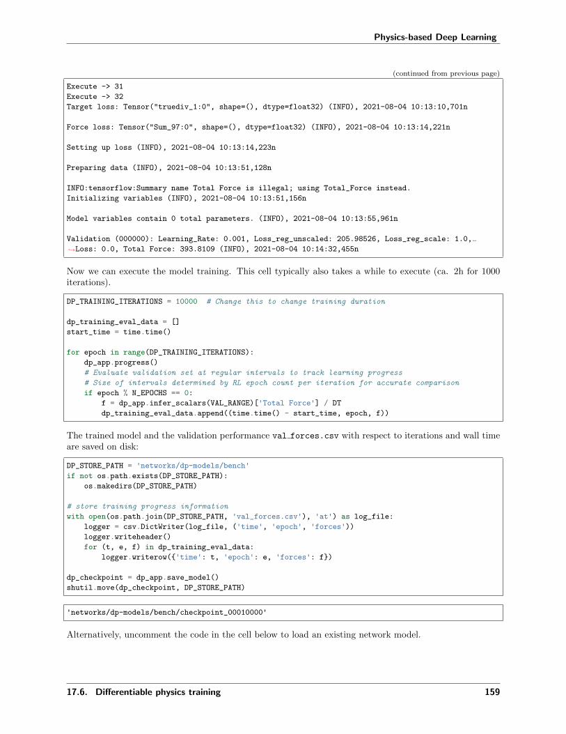
Physics-based Deep Learning
(continued from previous page)
Execute -> 31
Execute -> 32
Target loss: Tensor("truediv_1:0", shape=(), dtype=float32) (INFO), 2021-08-04 10:13:10,701n
Force loss: Tensor("Sum_97:0", shape=(), dtype=float32) (INFO), 2021-08-04 10:13:14,221n
Setting up loss (INFO), 2021-08-04 10:13:14,223n
Preparing data (INFO), 2021-08-04 10:13:51,128n
INFO:tensorflow:Summary name Total Force is illegal; using Total_Force instead.
Initializing variables (INFO), 2021-08-04 10:13:51,156n
Model variables contain 0 total parameters. (INFO), 2021-08-04 10:13:55,961n
Validation (000000): Learning_Rate: 0.001, Loss_reg_unscaled: 205.98526, Loss_reg_scale: 1.0,
→˓Loss: 0.0, Total Force: 393.8109 (INFO), 2021-08-04 10:14:32,455n
Now we can execute the model training. This cell typically also takes a while to execute (ca. 2h for 1000iterations).
DP_TRAINING_ITERATIONS = 10000 # Change this to change training duration
dp_training_eval_data = []
start_time = time.time()
for epoch in range(DP_TRAINING_ITERATIONS):
dp_app.progress()
# Evaluate validation set at regular intervals to track learning progress
# Size of intervals determined by RL epoch count per iteration for accurate comparison
if epoch % N_EPOCHS == 0:
f = dp_app.infer_scalars(VAL_RANGE)['Total Force'] / DT
dp_training_eval_data.append((time.time() - start_time, epoch, f))
The trained model and the validation performance val forces.csv with respect to iterations and wall timeare saved on disk:
DP_STORE_PATH = 'networks/dp-models/bench'if not os.path.exists(DP_STORE_PATH):
os.makedirs(DP_STORE_PATH)
# store training progress information
with open(os.path.join(DP_STORE_PATH, 'val_forces.csv'), 'at') as log_file:
logger = csv.DictWriter(log_file, ('time', 'epoch', 'forces'))logger.writeheader()
for (t, e, f) in dp_training_eval_data:
logger.writerow('time': t, 'epoch': e, 'forces': f)
dp_checkpoint = dp_app.save_model()
shutil.move(dp_checkpoint, DP_STORE_PATH)
'networks/dp-models/bench/checkpoint_00010000'
Alternatively, uncomment the code in the cell below to load an existing network model.
17.6. Differentiable physics training 159

Physics-based Deep Learning
# dp_path = 'PDE-Control-RL/networks/dp-models/bench/checkpoint_00020000/'# networks_to_load = ['OP2', 'OP4', 'OP8', 'OP16', 'OP32']
# dp_app.load_checkpoints(net: dp_path for net in networks_to_load)
Similar to the RL version, the next cell plots an example to visually show how well the DP-based modeldoes. The leftmost plot again shows the learned results, this time of the DP-based model. Like above, theother two show the ground truth and the natural evolution.
dp_frames = dp_app.infer_all_frames(TEST_RANGE)
dp_frames = [s.burgers.velocity.data for s in dp_frames]
_, gt_frames, unc_frames = rl_trainer.infer_test_set_frames()
TEST_SAMPLE = 0 # Change this to display a reconstruction of another scene
fig, axs = plt.subplots(1, 3, figsize=(18.9, 9.6))
axs[0].set_title("Differentiable Physics")
axs[1].set_title("Ground Truth")
axs[2].set_title("Uncontrolled")
for plot in axs:
plot.set_ylim(-2, 2)
plot.set_xlabel('x')plot.set_ylabel('u(x)')
for frame in range(0, STEP_COUNT + 1):
frame_color = bplt.gradient_color(frame, STEP_COUNT+1)
axs[0].plot(dp_frames[frame][TEST_SAMPLE,:], color=frame_color, linewidth=0.8)
axs[1].plot(gt_frames[frame][TEST_SAMPLE,:], color=frame_color, linewidth=0.8)
axs[2].plot(unc_frames[frame][TEST_SAMPLE,:], color=frame_color, linewidth=0.8)
"See the documentation of nn.Upsample for details.".format(mode)
The trained DP model also reconstructs the original trajectories closely. Furthermore, the generated results
160 Chapter 17. Controlling Burgers’ Equation with Reinforcement Learning

Physics-based Deep Learning
seem less noisy than using the RL agent.
With this, we have an RL and a DP version, which we can compare in more detail in the next section.
17.7 Comparison between RL and DP
Next, the results of both methods are compared in terms of visual quality of the resulting trajectories as wellas quantitatively via the amount of generated forces. The latter provides insights about the performance ofeither approaches as both methods aspire to minimize this metric during training. This is also importantas the task is trivially solved by applying a huge force at the last time step. Therefore, an ideal solutiontakes into account the dynamics of the PDE to apply as little forces as possible. Hence, this metric is a verygood one to measure how well the network has learned about the underlying physical environment (Burgersequation in this example).
import utils
import pandas as pd
17.7.1 Trajectory comparison
To compare the resulting trajectories, we generate trajectories from the test set with either method. Also,we collect the ground truth simulations and the natural evolution of the test set fields.
rl_frames, gt_frames, unc_frames = rl_trainer.infer_test_set_frames()
dp_frames = dp_app.infer_all_frames(TEST_RANGE)
dp_frames = [s.burgers.velocity.data for s in dp_frames]
frames =
(0, 0): ('Ground Truth', gt_frames),
(0, 1): ('Uncontrolled', unc_frames),
(1, 0): ('Reinforcement Learning', rl_frames),
(1, 1): ('Differentiable Physics', dp_frames),
"See the documentation of nn.Upsample for details.".format(mode)
TEST_SAMPLE = 0 # Specifies which sample of the test set should be displayed
def plot(axs, xy, title, field):
axs[xy].set_ylim(-2, 2); axs[xy].set_title(title)
axs[xy].set_xlabel('x'); axs[xy].set_ylabel('u(x)')label = 'Initial state (red), final state (blue)'for step_idx in range(0, STEP_COUNT + 1):
color = bplt.gradient_color(step_idx, STEP_COUNT+1)
axs[xy].plot(
field[step_idx][TEST_SAMPLE].squeeze(), color=color, linewidth=0.8, label=label)
label = None
axs[xy].legend()
fig, axs = plt.subplots(2, 2, figsize=(12.8, 9.6))
for xy in frames:
plot(axs, xy, *frames[xy])
17.7. Comparison between RL and DP 161

Physics-based Deep Learning
This diagram connects the two plots shown above after each training. Here we again see that the differen-tiable physics approach seems to generate less noisy trajectories than the RL agent, while both manage toapproximate the ground truth.
17.7.2 Comparison of exerted forces
Next, we compute the forces the approaches have generated and applied for the test set trajectories.
gt_forces = utils.infer_forces_sum_from_frames(
gt_frames, DOMAIN, DIFFUSION_SUBSTEPS, VISCOSITY, DT
)
dp_forces = utils.infer_forces_sum_from_frames(
dp_frames, DOMAIN, DIFFUSION_SUBSTEPS, VISCOSITY, DT
)
rl_forces = rl_trainer.infer_test_set_forces()
Sanity check - maximum deviation from target state: 0.000000
Sanity check - maximum deviation from target state: 0.000011
"See the documentation of nn.Upsample for details.".format(mode)
At first, we will compare the total sum of the forces that are generated by the RL and DP approaches andcompare them to the ground truth.
162 Chapter 17. Controlling Burgers’ Equation with Reinforcement Learning

Physics-based Deep Learning
plt.figure(figsize=(8, 6))
plt.bar(
["Reinforcement Learning", "Differentiable Physics", "Ground Truth"],
[np.sum(rl_forces), np.sum(dp_forces), np.sum(gt_forces)],
color = ["#0065bd", "#e37222", "#a2ad00"],
align='center', label='Absolute forces comparison' )
<BarContainer object of 3 artists>
As visualized in these bar plots, the DP approach learns to apply slightly lower forces than the RL model.As both methods are on-par in terms of how well they reach the final target states, this is the main quantitywe use to compare the performance of both methods.
In the following, the forces generated by the methods are also visually compared to the ground truth ofthe respective sample. Dots placed above the blue line denote stronger forces in the analyzed deep learningapproach than in the ground truth and vice versa.
plt.figure(figsize=(12, 9))
plt.scatter(gt_forces, rl_forces, color="#0065bd", label='RL')plt.scatter(gt_forces, dp_forces, color="#e37222", label='DP')plt.plot([x * 100 for x in range(15)], [x * 100 for x in range(15)], color="#a2ad00", label='Same→˓forces as original')plt.xlabel('ground truth'); plt.ylabel('reconstruction')plt.xlim(0, 1200); plt.ylim(0, 1200); plt.grid(); plt.legend()
17.7. Comparison between RL and DP 163

Physics-based Deep Learning
<matplotlib.legend.Legend at 0x7f4cbc6d5090>
The graph shows that the orange dots of the DP training run are in general closer to the diagonal - i.e., thisnetwork learned to generate forces that are closer to the ground truth values.
The following plot displays the performance of all reinforcement learning, differentiable physics and groundtruth with respect to individual samples.
w=0.25; plot_count=20 # How many scenes to show
plt.figure(figsize=(12.8, 9.6))
plt.bar( [i - w for i in range(plot_count)], rl_forces[:plot_count], color="#0065bd", width=w,
→˓align='center', label='RL' )
plt.bar( [i for i in range(plot_count)], dp_forces[:plot_count], color="#e37222", width=w,
→˓align='center', label='DP' )
plt.bar( [i + w for i in range(plot_count)], gt_forces[:plot_count], color="#a2ad00", width=w,
→˓align='center', label='GT' )
plt.xlabel('Scenes'); plt.xticks(range(plot_count))
plt.ylabel('Forces'); plt.legend(); plt.show()
164 Chapter 17. Controlling Burgers’ Equation with Reinforcement Learning

Physics-based Deep Learning
17.8 Training progress comparison
Although the quality of the control in terms of force magnitudes is the primary goal of the setup above,there are interesting differences in terms of how both methods behave at training time. The main differenceof the physics-unaware RL training and the DP approach with its tightly coupled solver is that the latterresults in a significantly faster convergence. I.e., the gradients provided by the numerical solver give a muchbetter learning signal than the undirected exploration of the RL process. The behavior of the RL training,on the other hand, can in part be ascribed to the on-policy nature of training data collection and to the“brute-force” exploration of the reinforcement learning technique.
The next cell visualizes the training progress of both methods with respect to wall time.
def get_dp_val_set_forces(experiment_path):
path = os.path.join(experiment_path, 'val_forces.csv')table = pd.read_csv(path)
return list(table['time']), list(table['epoch']), list(table['forces'])
rl_w_times, rl_step_nums, rl_val_forces = rl_trainer.get_val_set_forces_data()
dp_w_times, dp_epochs, dp_val_forces = get_dp_val_set_forces(DP_STORE_PATH)
plt.figure(figsize=(12, 5))
plt.plot(np.array(rl_w_times) / 3600, rl_val_forces, color="#0065bd", label='RL')plt.plot(np.array(dp_w_times) / 3600, dp_val_forces, color="#e37222", label='DP')
(continues on next page)
17.8. Training progress comparison 165

Physics-based Deep Learning
(continued from previous page)
plt.xlabel('Wall time (hours)'); plt.ylabel('Forces')plt.ylim(0, 1500); plt.grid(); plt.legend()
<matplotlib.legend.Legend at 0x7f4cbc595c50>
To conclude, the PPO reinforcement learning exerts higher forces in comparison to the differentiable physicsapproach. Hence, PPO yields a learned solution with slightly inferior quality. Additionally, the time neededfor convergence is significantly higher in the RL case (both in terms of wall time and training iterations).
17.9 Next steps
• See how different values for hyperparameters, such as learning rate, influence the training process
• Work with fields of different resolution and see how the two approaches then compare to each other.Larger resolutions make the physical dynamics more complex, and hence harder to control
• Use trained models in settings with different environment parameters (e.g. viscosity, dt) and test howwell they generalize
166 Chapter 17. Controlling Burgers’ Equation with Reinforcement Learning
Part VI
PBDL and Uncertainty
167


CHAPTER
EIGHTEEN
INTRODUCTION TO POSTERIOR INFERENCE
We should keep in mind that for all measurements, models, and discretizations we have uncertainties. Formeasurements and observations, this typically appears in the form of measurement errors. Model equationsequations, on the other hand, usually encompass only parts of a system we’re interested in (leaving theremainder as an uncertainty), while for numerical simulations we inherently introduce discretization errors.So a very important question to ask here is how we can be sure that an answer we obtain is the correct one.From a statisticians viewpoint, we’d like to know the posterior pobability distribution, a distribution thatcaptures possible uncertainties we have about our model or data.
18.1 Uncertainty
This admittedly becomes even more difficult in the context of machine learning: we’re typically facing thetask of approximating complex and unknown functions. From a probabilistic perspective, the standardprocess of training an NN here yields a maximum likelihood estimation (MLE) for the parameters of thenetwork. However, this MLE viewpoint does not take any of the uncertainties mentioned above into account:for DL training, we likewise have a numerical optimization, and hence an inherent approximation error anduncertainty regarding the learned representation. Ideally, we should reformulate our the learning processsuch that it takes its own uncertainties into account, and it should make posterior inference possible, i.e.learn to produce the full output distribution. However, this turns out to be an extremely difficult task.
This is where so-called Bayesian neural network (BNN) approaches come into play. They allow for a formof posterior inference by making assumptions about the probability distributions of individual parameters ofthe network. This gives a distribution for the parameters, with which we can evaluate the network multipletimes to obtain different versions of the output, and in this way sample the distribution of the output.
Nonetheless, the task remains very challenging. Training a BNN is typically significantly more difficult thantraining a regular NN. This should come as no surprise, as we’re trying to learn something fundamentallydifferent here: a full probability distribution instead of a point estimate. (All previous chapters “just” dealtwith learning such point estimates, and the tasks were still far from trivial.)
Aleatoric and Epistemic Uncertainty
Although we won’t go into detail within the scope of this book, many works distinguish two types ofuncertainty which are important to mention here:
• Aleatoric uncertainty denotes uncertainty within the data, e.g., noise in measurements.
• Epistemic uncertainty, on the other hand, describes uncertainties within a model such as a trainedneural network.
In the following we’ll primarily target epistemic uncertainty via posterior inference. However, as a word ofcaution: if they appear together, the different kinds of uncertainties (the two types above are not exhaustive)
169

Physics-based Deep Learning
are very difficult to disentangle in practice.
18.2 Introduction to Bayesian Neural Networks
In order to combine posterior inference with Neural Networks, we can use standard techniques from BayesianModeling and combine them with the Deep Learning machinery. In Bayesian Modeling, we aim at learningdistributions over the model parameters instead of these fixed point estimates. In the case of NNs, the modelparameters are the weights and biases, summarized by 𝜃, for a neural network 𝑓 . Our goal is therefore tolearn a so-called posterior distribution 𝑝(𝜃|𝐷) from the data 𝐷, which captures the uncertainty we haveabout the networks weights and biases after observing the data 𝐷. This posterior distribution is the centralquantity of interest here: if we can estimate it reasonably well, we can use it to make good predictions, butalso assess uncertainties related to those predictions. For both objectives it is necessary to marginalize overthe posterior distribution, i.e. integrate it out. A single prediction for input 𝑥𝑖 can for example be obtainedvia
𝑦𝑖 =
∫𝑓(𝑥𝑖; 𝜃) 𝑝(𝜃|𝐷) 𝑑𝜃
Similarly, one can for instance compute the standard deviation in order to assess a measure of uncertaintyover the prediction 𝑦𝑖.
18.3 Prior distributions
In order to obtain the required posterior distribution, in Bayesian modeling one first has to define a priordistribution 𝑝(𝜃) over the network parameters. This prior distribution should encompass the knowledge wehave about the network weights before training the model. We for instance know that the weights of neuralnetworks are usually rather small and can be both positive and negative. Centered normal distributionswith some small variance parameter are therefore a standard choice. For computational simplicity, they aretypically also assumed to be independent from another. When observing data 𝐷, the prior distribution overthe weights is updated to the posterior according to Bayes rule:
𝑝(𝜃|𝐷) =𝑝(𝐷|𝜃)𝑝(𝜃)
𝑝(𝐷).
This is, we update our a-priori knowledge after observing data, i.e. we learn from data. The computationrequired for the Bayesian update is usually intractable, especially when dealing with non-trivial networkarchitectures. Therefore, the posterior 𝑝(𝜃|𝐷) is approximated with an easy-to-evaluate variational distribu-tion 𝑞𝜑(𝜃), parametrized by 𝜑. Again, independent Normal distributions are typically used for each weight.Hence, the parameters 𝜑 contain all mean and variance parameters 𝜇, 𝜎 of those normal distributions. Theoptimization goal is then to find a distribution 𝑞𝜑(𝜃) that is close to the true posterior. One way of assessingthis closeness is the KL-divergence, a method used widely in practice for measuring the similarity of twodistributions.
170 Chapter 18. Introduction to Posterior Inference

Physics-based Deep Learning
18.4 Evidence lower bound
We cannot directly minimize the KL-divergence between approximate and true posterior 𝐾𝐿(𝑞𝜑(𝜃)||𝑝(𝜃|𝐷),because we do not have access to the true posterior distribution. It is however possible to show that one canequivalently maximize the so-called evidence lower bound (ELBO), a quantity well known from variationalinference:
ℒ(𝜑) = 𝐸𝑞𝜑 [log(𝑝(𝐷|𝜃))] −𝐾𝐿(𝑞𝜑(𝜃)||𝑝(𝜃)) ,
The ELBO (or negative ELBO, if one prefers to minimize instead of maximize) is the optimization objectivefor BNNs. The first term is an expected log-likelihood of the data. Maximizing it means explaining the dataas well as possible. In practice, the log-likelihood is often a conventional loss functions like mean squarederror (note that MSE can be seen as negative log-likelihood for normal noise with unit variance). The secondterm is the negative KL-divergence between the approximate posterior and the prior. For suitable prior andapproximate posterior choices (like the ones above), this term can be computed analytically. Maximizing itmeans encouraging the approximate network weight distributions to stay close to the prior distribution. Inthat sense, the two terms of the ELBO have opposite goals: The first term encourages the model to explainthe data as well as possible, whereas the second term encourages the model to stay close to the (random)prior distributions, which implies randomness and regularization.
The expectation of the log-likelihood is typically not available in analytical form, but can be approximatedin several ways. One can, for instance, use Monte-Carlo sampling and draw 𝑆 samples from 𝑞𝜑(𝜃). The
expectation is then approximated via 1𝑆
∑𝑆𝑠=1 log(𝑝(𝐷|𝜃𝑠). In practice, even a single sample, i.e. 𝑆 = 1
can be enough. Furthermore, the expectation of the log-likelihood is typically not evaluated on the wholedataset, but approximated by a batch of data 𝐷𝑏𝑎𝑡𝑐ℎ, which enables the use of batch-wise stochastic gradientdescent.
18.5 The BNN training loop
For 𝑆 = 1, one iteration of the training loop then boils down to
1. sampling a batch of data 𝐷𝑏𝑎𝑡𝑐ℎ
2. sampling network weights and biases from 𝑞𝜑(𝜃)
3. forwarding the batch of data through the network according to the sampled weights
4. evaluating the ELBO
5. backpropagating the ELBO through the network and updating 𝜑
If 𝑆 > 1, steps 2 and 3 have to be repeated 𝑆 times in order to compute the ELBO. In that sense, traininga variational BNN is fairly similar to training a conventional NN: We still use SGD and forward-backwardpasses to optimize our loss function. Only that now we are optimizing over distributions instead of singlevalues. If you are curious on how one can backpropagate through distributions, you can, e.g., read about ithere, and a more detailed introduction to Bayesian Neural Networks is available in Y. Gals thesis, in chapters2 & 3.
18.4. Evidence lower bound 171
Physics-based Deep Learning
18.6 Dropout as alternative
Previous work has shown that using dropout is mathematically equivalent to an approximation to theprobabilistic deep Gaussian process. Furthermore, for a specific prior (satisfying the so-called KL-condition)and specific approximate posterior choice (a product of Bernoulli distributions), training a neural networkwith dropout and L2 regularization and training a variational BNN results in an equivalent optimizationprocedure. In other words, dropout neural networks are a form of Bayesian neural networks.
Obtaining uncertainty estimates is then as easy as training a conventional neural network with dropoutand extending dropout, which traditionally has only been used during the training phase, to the predictionphase. This will lead to the predictions being random (because dropout will randomly drop some of theactivations), which allows us to compute average and standard deviation statistics for single samples fromthe dataset, just like for the variational BNN case. It is an ongoing discussion in the field whether variationalor dropout-based methods are preferable.
18.7 A practical example
As a first real example for posterior inference with variational BNNs, let’s revisit the case of turbulent flowsaround airfoils, from Supervised training for RANS flows around airfoils. However, in contrast to the pointestimate learned in this section, we’ll now aim for learning the full posterior.
172 Chapter 18. Introduction to Posterior Inference

CHAPTER
NINETEEN
RANS AIRFOIL FLOWS WITH BAYESIAN NEURAL NETS
19.1 Overview
We are now considering the same setup as in the notebook Supervised training for RANS flows aroundairfoils: A turbulent airflow around wing profiles, for which we’d like to know the average motion andpressure distribution around this airfoil for different Reynolds numbers and angles of attack. In the earliernotebook, we tackled this by completely bypassing any physical solver and instead training a neural networkthat learns the quantities of interest. Now, we want to extend this approach to the variational BayesianNeural Networks (BNNs) of the previous section. In contrast to traditional networks, that learn a singlepoint estimate for each weight value, BNNs aim at learning a distribution over each weight parameter(e.g. a Gaussian with mean 𝜇 and variance 𝜎2). During a forward-pass, each parameter in the network isthen sampled from its corresponding approximate posterior distribution 𝑞𝜑(𝜃). In that sense, the networkparameters themselves are random variables and each forward pass becomes stochastic, because for a giveninput the predictions will vary with every forward-pass. This allows to assess how uncertain the network is:If the predictions vary a lot, we think that the network is uncertain about its output. [run in colab]
19.1.1 Read in Data
Like in the previous notebook we’ll skip the data generation process. This example is adapted from theDeep-Flow-Prediction codebase, which you can check out for details. Here, we’ll simply download a smallset of training data generated with a Spalart-Almaras RANS simulation in OpenFOAM.
import numpy as np
import os.path, random
# get training data: as in the previous supervised example, either download or use gdrive
dir = "./"
if True:
if not os.path.isfile('data-airfoils.npz'):import requests
print("Downloading training data (300MB), this can take a few minutes the first time...")
with open("data-airfoils.npz", 'wb') as datafile:
resp = requests.get('https://dataserv.ub.tum.de/s/m1615239/download?path=%2F &files=dfp-→˓data-400.npz', verify=False)
datafile.write(resp.content)
else: # cf supervised airfoil code:
from google.colab import drive
drive.mount('/content/gdrive')dir = "./gdrive/My Drive/"
npfile=np.load(dir+'data-airfoils.npz')(continues on next page)
173
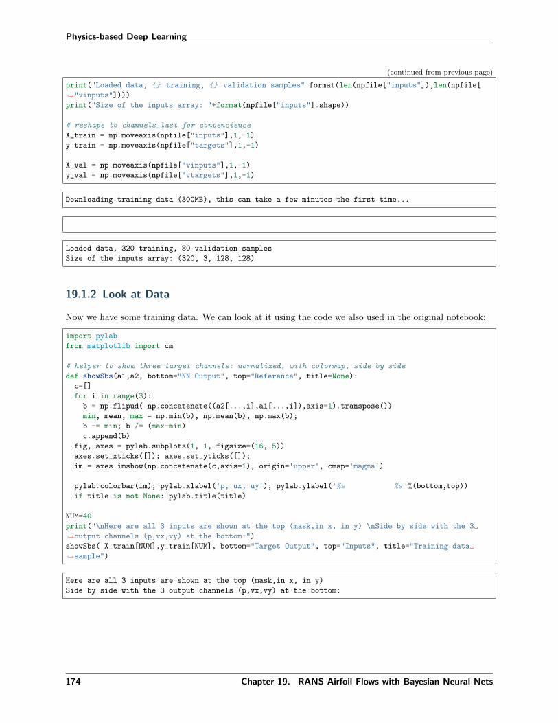
Physics-based Deep Learning
(continued from previous page)
print("Loaded data, training, validation samples".format(len(npfile["inputs"]),len(npfile[
→˓"vinputs"])))
print("Size of the inputs array: "+format(npfile["inputs"].shape))
# reshape to channels_last for convencience
X_train = np.moveaxis(npfile["inputs"],1,-1)
y_train = np.moveaxis(npfile["targets"],1,-1)
X_val = np.moveaxis(npfile["vinputs"],1,-1)
y_val = np.moveaxis(npfile["vtargets"],1,-1)
Downloading training data (300MB), this can take a few minutes the first time...
Loaded data, 320 training, 80 validation samples
Size of the inputs array: (320, 3, 128, 128)
19.1.2 Look at Data
Now we have some training data. We can look at it using the code we also used in the original notebook:
import pylab
from matplotlib import cm
# helper to show three target channels: normalized, with colormap, side by side
def showSbs(a1,a2, bottom="NN Output", top="Reference", title=None):
c=[]
for i in range(3):
b = np.flipud( np.concatenate((a2[...,i],a1[...,i]),axis=1).transpose())
min, mean, max = np.min(b), np.mean(b), np.max(b);
b -= min; b /= (max-min)
c.append(b)
fig, axes = pylab.subplots(1, 1, figsize=(16, 5))
axes.set_xticks([]); axes.set_yticks([]);
im = axes.imshow(np.concatenate(c,axis=1), origin='upper', cmap='magma')
pylab.colorbar(im); pylab.xlabel('p, ux, uy'); pylab.ylabel('%s %s '%(bottom,top))if title is not None: pylab.title(title)
NUM=40
print("\nHere are all 3 inputs are shown at the top (mask,in x, in y) \nSide by side with the 3
→˓output channels (p,vx,vy) at the bottom:")
showSbs( X_train[NUM],y_train[NUM], bottom="Target Output", top="Inputs", title="Training data
→˓sample")
Here are all 3 inputs are shown at the top (mask,in x, in y)
Side by side with the 3 output channels (p,vx,vy) at the bottom:
174 Chapter 19. RANS Airfoil Flows with Bayesian Neural Nets

Physics-based Deep Learning
Not surprisingly, the data still looks the same. For details, please check out the description in Supervisedtraining for RANS flows around airfoils.
19.1.3 Neural Network Definition
Now let’s look at how we can implement BNNs. Instead of PyTorch, we will use TensorFlow, in particularthe extension TensorFlow Probability, which has easy-to-implement probabilistic layers. Like in the othernotebook, we use a U-Net structure consisting of Convolutional blocks with skip-layer connections. Fornow, we only want to set up the decoder, i.e. second part of the U-Net as bayesian. For this, we will takeadvantage of TensorFlows flipout layers (in particular, the convolutional implementation).
In a forward pass, those layers automatically sample from the current posterior distribution and store theKL-divergence between prior and posterior in model.losses. One can specify the desired divergence measure(typically KL-divergence) and modify the prior and approximate posterior distributions, if other than normaldistributions are desired. Other than that, the flipout layers can be used just like regular layers in sequentialarchitectures. The code below implements a single convolutional block of the U-Net:
import tensorflow as tf
import tensorflow_probability.python.distributions as tfd
from tensorflow.keras import Sequential
from tensorflow.keras.initializers import RandomNormal
from tensorflow.keras.layers import Input, Conv2D, Conv2DTranspose,UpSampling2D,
→˓BatchNormalization, ReLU, LeakyReLU, SpatialDropout2D, MaxPooling2D
from tensorflow_probability.python.layers import Convolution2DFlipout
from tensorflow.keras.models import Model
def tfBlockUnet(filters=3, transposed=False, kernel_size=4, bn=True, relu=True, pad="same",
→˓dropout=0., flipout=False,
kdf=None, name=''):(continues on next page)
19.1. Overview 175
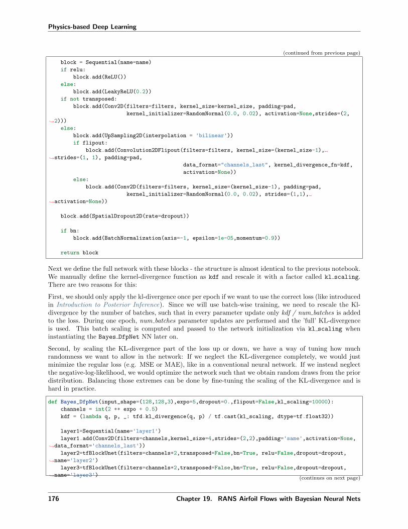
Physics-based Deep Learning
(continued from previous page)
block = Sequential(name=name)
if relu:
block.add(ReLU())
else:
block.add(LeakyReLU(0.2))
if not transposed:
block.add(Conv2D(filters=filters, kernel_size=kernel_size, padding=pad,
kernel_initializer=RandomNormal(0.0, 0.02), activation=None,strides=(2,
→˓2)))
else:
block.add(UpSampling2D(interpolation = 'bilinear'))if flipout:
block.add(Convolution2DFlipout(filters=filters, kernel_size=(kernel_size-1),
→˓strides=(1, 1), padding=pad,
data_format="channels_last", kernel_divergence_fn=kdf,
activation=None))
else:
block.add(Conv2D(filters=filters, kernel_size=(kernel_size-1), padding=pad,
kernel_initializer=RandomNormal(0.0, 0.02), strides=(1,1),
→˓activation=None))
block.add(SpatialDropout2D(rate=dropout))
if bn:
block.add(BatchNormalization(axis=-1, epsilon=1e-05,momentum=0.9))
return block
Next we define the full network with these blocks - the structure is almost identical to the previous notebook.We manually define the kernel-divergence function as kdf and rescale it with a factor called kl scaling.There are two reasons for this:
First, we should only apply the kl-divergence once per epoch if we want to use the correct loss (like introducedin Introduction to Posterior Inference). Since we will use batch-wise training, we need to rescale the Kl-divergence by the number of batches, such that in every parameter update only kdf / num batches is addedto the loss. During one epoch, num batches parameter updates are performed and the ’full’ KL-divergenceis used. This batch scaling is computed and passed to the network initialization via kl scaling wheninstantiating the Bayes DfpNet NN later on.
Second, by scaling the KL-divergence part of the loss up or down, we have a way of tuning how muchrandomness we want to allow in the network: If we neglect the KL-divergence completely, we would justminimize the regular loss (e.g. MSE or MAE), like in a conventional neural network. If we instead neglectthe negative-log-likelihood, we would optimize the network such that we obtain random draws from the priordistribution. Balancing those extremes can be done by fine-tuning the scaling of the KL-divergence and ishard in practice.
def Bayes_DfpNet(input_shape=(128,128,3),expo=5,dropout=0.,flipout=False,kl_scaling=10000):
channels = int(2 ** expo + 0.5)
kdf = (lambda q, p, _: tfd.kl_divergence(q, p) / tf.cast(kl_scaling, dtype=tf.float32))
layer1=Sequential(name='layer1')layer1.add(Conv2D(filters=channels,kernel_size=4,strides=(2,2),padding='same',activation=None,
→˓data_format='channels_last'))layer2=tfBlockUnet(filters=channels*2,transposed=False,bn=True, relu=False,dropout=dropout,
→˓name='layer2')layer3=tfBlockUnet(filters=channels*2,transposed=False,bn=True, relu=False,dropout=dropout,
→˓name='layer3')(continues on next page)
176 Chapter 19. RANS Airfoil Flows with Bayesian Neural Nets
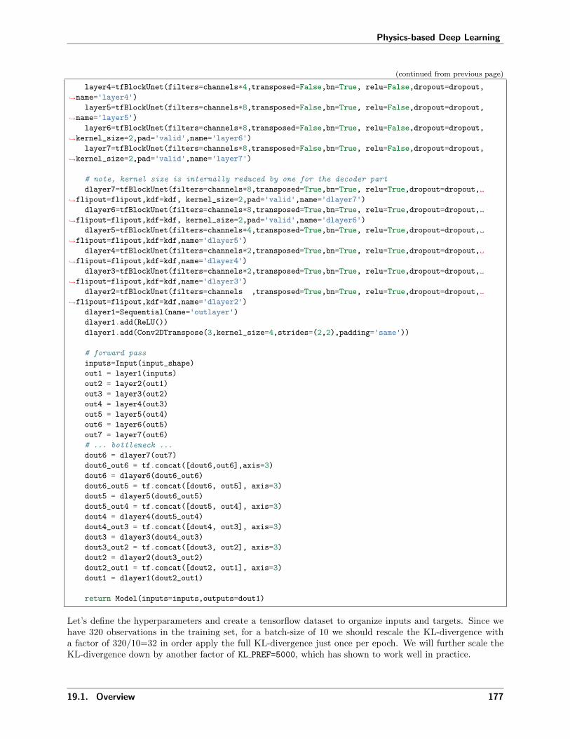
Physics-based Deep Learning
(continued from previous page)
layer4=tfBlockUnet(filters=channels*4,transposed=False,bn=True, relu=False,dropout=dropout,
→˓name='layer4')layer5=tfBlockUnet(filters=channels*8,transposed=False,bn=True, relu=False,dropout=dropout,
→˓name='layer5')layer6=tfBlockUnet(filters=channels*8,transposed=False,bn=True, relu=False,dropout=dropout,
→˓kernel_size=2,pad='valid',name='layer6')layer7=tfBlockUnet(filters=channels*8,transposed=False,bn=True, relu=False,dropout=dropout,
→˓kernel_size=2,pad='valid',name='layer7')
# note, kernel size is internally reduced by one for the decoder part
dlayer7=tfBlockUnet(filters=channels*8,transposed=True,bn=True, relu=True,dropout=dropout,
→˓flipout=flipout,kdf=kdf, kernel_size=2,pad='valid',name='dlayer7')dlayer6=tfBlockUnet(filters=channels*8,transposed=True,bn=True, relu=True,dropout=dropout,
→˓flipout=flipout,kdf=kdf, kernel_size=2,pad='valid',name='dlayer6')dlayer5=tfBlockUnet(filters=channels*4,transposed=True,bn=True, relu=True,dropout=dropout,
→˓flipout=flipout,kdf=kdf,name='dlayer5')dlayer4=tfBlockUnet(filters=channels*2,transposed=True,bn=True, relu=True,dropout=dropout,
→˓flipout=flipout,kdf=kdf,name='dlayer4')dlayer3=tfBlockUnet(filters=channels*2,transposed=True,bn=True, relu=True,dropout=dropout,
→˓flipout=flipout,kdf=kdf,name='dlayer3')dlayer2=tfBlockUnet(filters=channels ,transposed=True,bn=True, relu=True,dropout=dropout,
→˓flipout=flipout,kdf=kdf,name='dlayer2')dlayer1=Sequential(name='outlayer')dlayer1.add(ReLU())
dlayer1.add(Conv2DTranspose(3,kernel_size=4,strides=(2,2),padding='same'))
# forward pass
inputs=Input(input_shape)
out1 = layer1(inputs)
out2 = layer2(out1)
out3 = layer3(out2)
out4 = layer4(out3)
out5 = layer5(out4)
out6 = layer6(out5)
out7 = layer7(out6)
# ... bottleneck ...
dout6 = dlayer7(out7)
dout6_out6 = tf.concat([dout6,out6],axis=3)
dout6 = dlayer6(dout6_out6)
dout6_out5 = tf.concat([dout6, out5], axis=3)
dout5 = dlayer5(dout6_out5)
dout5_out4 = tf.concat([dout5, out4], axis=3)
dout4 = dlayer4(dout5_out4)
dout4_out3 = tf.concat([dout4, out3], axis=3)
dout3 = dlayer3(dout4_out3)
dout3_out2 = tf.concat([dout3, out2], axis=3)
dout2 = dlayer2(dout3_out2)
dout2_out1 = tf.concat([dout2, out1], axis=3)
dout1 = dlayer1(dout2_out1)
return Model(inputs=inputs,outputs=dout1)
Let’s define the hyperparameters and create a tensorflow dataset to organize inputs and targets. Since wehave 320 observations in the training set, for a batch-size of 10 we should rescale the KL-divergence witha factor of 320/10=32 in order apply the full KL-divergence just once per epoch. We will further scale theKL-divergence down by another factor of KL PREF=5000, which has shown to work well in practice.
19.1. Overview 177

Physics-based Deep Learning
Furthermore, we will define a function that implements learning rate decay. Intuitively, this allows theoptimization to be more precise (by making smaller steps) in later epochs, while still making fast progress(by making bigger steps) in the first epochs.
import math
import matplotlib.pyplot as plt
BATCH_SIZE=10
LR=0.001
EPOCHS = 120
KL_PREF = 5000
dataset = tf.data.Dataset.from_tensor_slices((X_train, y_train)).shuffle(len(X_train),
seed=46168531, reshuffle_each_iteration=False).batch(BATCH_SIZE, drop_remainder=False)
def compute_lr(i, epochs, minLR, maxLR):
if i < epochs * 0.5:
return maxLR
e = (i / float(epochs) - 0.5) * 2.
# rescale second half to min/max range
fmin = 0.
fmax = 6.
e = fmin + e * (fmax - fmin)
f = math.pow(0.5, e)
return minLR + (maxLR - minLR) * f
We can visualize the learning rate decay: We start off with a constant rate and after half of the EPOCHS westart to decay it exponentially, until arriving at half of the original learning rate.
lrs=[compute_lr(i, EPOCHS, 0.5*LR,LR) for i in range(EPOCHS)]
plt.plot(lrs)
plt.xlabel('Iteration')plt.ylabel('Learning Rate')
Text(0, 0.5, 'Learning Rate')
178 Chapter 19. RANS Airfoil Flows with Bayesian Neural Nets

Physics-based Deep Learning
Let’s initialize the network. Here we’re finally computing the kl scaling factor via KL PREF and the batchsize.
from tensorflow.keras.optimizers import RMSprop, Adam
model=Bayes_DfpNet(expo=4,flipout=True,kl_scaling=KL_PREF*len(X_train)/BATCH_SIZE)
optimizer = Adam(learning_rate=LR, beta_1=0.5,beta_2=0.9999)
num_params = np.sum([np.prod(v.get_shape().as_list()) for v in model.trainable_variables])
print('The Bayesian U-Net has parameters.'.format(num_params))
The Bayesian U-Net has 846787 parameters.
In general, flipout layers come with twice as many parameters as their conventional counterparts, sinceinstead of a single point estimate one has to learn both mean and variance parameters for the Gaussianposterior of the weights. As we only have flipout layers for the decoder part here, the resulting model has846787 parameters, compared to the 585667 of the conventional NN.
19.2 Training
Now we are ready to run the training! Note that this might take a while (typically around 4 hours), as theflipout layers are significantly slower to train compared to regular layers.
from tensorflow.keras.losses import mae
import math
kl_losses=[]
mae_losses=[]
(continues on next page)
19.2. Training 179

Physics-based Deep Learning
(continued from previous page)
total_losses=[]
mae_losses_vali=[]
for epoch in range(EPOCHS):
# compute learning rate - decay is implemented
currLr = compute_lr(epoch,EPOCHS,0.5*LR,LR)
if currLr < LR:
tf.keras.backend.set_value(optimizer.lr, currLr)
# iterate through training data
kl_sum = 0
mae_sum = 0
total_sum=0
for i, traindata in enumerate(dataset, 0):
# forward pass and loss computation
with tf.GradientTape() as tape:
inputs, targets = traindata
prediction = model(inputs, training=True)
loss_mae = tf.reduce_mean(mae(prediction, targets))
kl=sum(model.losses)
loss_value=kl+tf.cast(loss_mae, dtype='float32')# backpropagate gradients and update parameters
gradients = tape.gradient(loss_value, model.trainable_variables)
optimizer.apply_gradients(zip(gradients, model.trainable_variables))
# store losses per batch
kl_sum += kl
mae_sum += tf.reduce_mean(loss_mae)
total_sum+=tf.reduce_mean(loss_value)
# store losses per epoch
kl_losses+=[kl_sum/len(dataset)]
mae_losses+=[mae_sum/len(dataset)]
total_losses+=[total_sum/len(dataset)]
# validation
outputs = model.predict(X_val)
mae_losses_vali += [tf.reduce_mean(mae(y_val, outputs))]
if epoch<3 or epoch%20==0:
print('Epoch / , total loss: :.3f , KL loss: :.3f , MAE loss: :.4f , MAE loss
→˓vali: :.4f '.format(epoch, EPOCHS, total_losses[-1], kl_losses[-1], mae_losses[-1], mae_losses_
→˓vali[-1]))
Epoch 0/120, total loss: 4.265, KL loss: 4.118, MAE loss: 0.1464, MAE loss vali: 0.0872
Epoch 1/120, total loss: 4.159, KL loss: 4.089, MAE loss: 0.0706, MAE loss vali: 0.0691
Epoch 2/120, total loss: 4.115, KL loss: 4.054, MAE loss: 0.0610, MAE loss vali: 0.0589
Epoch 20/120, total loss: 3.344, KL loss: 3.315, MAE loss: 0.0291, MAE loss vali: 0.0271
Epoch 40/120, total loss: 2.495, KL loss: 2.471, MAE loss: 0.0245, MAE loss vali: 0.0242
Epoch 60/120, total loss: 1.712, KL loss: 1.689, MAE loss: 0.0228, MAE loss vali: 0.0208
Epoch 80/120, total loss: 1.190, KL loss: 1.169, MAE loss: 0.0212, MAE loss vali: 0.0200
Epoch 100/120, total loss: 0.869, KL loss: 0.848, MAE loss: 0.0208, MAE loss vali: 0.0203
The BNN is trained! Let’s look at the loss. Since the loss consists of two separate parts, it is helpful tomonitor both parts (MAE and KL).
180 Chapter 19. RANS Airfoil Flows with Bayesian Neural Nets

Physics-based Deep Learning
fig,axs=plt.subplots(ncols=3,nrows=1,figsize=(20,4))
axs[0].plot(kl_losses,color='red')axs[0].set_title('KL Loss (Train)')axs[1].plot(mae_losses,color='blue',label='train')axs[1].plot(mae_losses_vali,color='green',label='val')axs[1].set_title('MAE Loss'); axs[1].legend()
axs[2].plot(total_losses,label='Total',color='black')axs[2].plot(kl_losses,label='KL',color='red')axs[2].plot(mae_losses,label='MAE',color='blue')axs[2].set_title('Total Train Loss'); axs[2].legend()
<matplotlib.legend.Legend at 0x7f6285c60490>
This way, we can double-check if minimizing one part of the loss comes at the cost of increasing the other.For our case, we observe that both parts decrease smoothly. In particular, the MAE loss is not increasingfor the validation set, indicating that we are not overfitting.
It is good practice to double-check how many layers added KL-losses. We can inspect model.losses for that.Since the decoder consists of 6 sequential blocks with flipout layers, we expect 6 entries in model.losses.
# there should be 6 entries in model.losses since we have 6 blocks with flipout layers in our model
print('There are entries in model.losses'.format(len(model.losses)))print(model.losses)
There are 6 entries in model.losses
[<tf.Tensor: shape=(), dtype=float32, numpy=0.03536303>, <tf.Tensor: shape=(), dtype=float32,
→˓numpy=0.06506929>, <tf.Tensor: shape=(), dtype=float32, numpy=0.2647468>, <tf.Tensor: shape=(),
→˓dtype=float32, numpy=0.09337218>, <tf.Tensor: shape=(), dtype=float32, numpy=0.0795429>, <tf.
→˓Tensor: shape=(), dtype=float32, numpy=0.075103864>]
Now let’s visualize how the BNN performs for unseen data from the validation set. Ideally, we would like tointegrate out the parameters 𝜃, i.e. marginalize in order to obtain a prediction. Since this is again hard torealize analytically, one usually approximates the integral via sampling from the posterior:
𝑦𝑖 =
∫𝑓(𝑥𝑖; 𝜃)𝑞𝜑(𝜃)𝑑𝜃 ≈ 1
𝑅
𝑅∑𝑟=1
𝑓(𝑥𝑖; 𝜃𝑟)
where each 𝜃𝑟 is drawn from 𝑞𝜑(𝜃). In practice, this just means performing 𝑅 forward passes for each input𝑥𝑖 and computing the average. In the same spirit, one can obtain the standard deviation as a measure ofuncertainty: 𝜎2
𝑖 = 1𝑅−1
∑𝑅𝑟=1(𝑓(𝑥𝑖; 𝜃) − 𝑦𝑖)
2.
Please note that both 𝑦𝑖 and 𝜎2𝑖 still have shape 128× 128× 3, i.e. the mean and variance computations are
performed per-pixel (but might be aggregated to a global measure afterwards).
19.2. Training 181

Physics-based Deep Learning
REPS=20
preds=np.zeros(shape=(REPS,)+X_val.shape)
for rep in range(REPS):
preds[rep,:,:,:,:]=model.predict(X_val)
preds_mean=np.mean(preds,axis=0)
preds_std=np.std(preds,axis=0)
Before inspecting the mean and standard deviation computed in the previous cell, let’s visualize one of theoutputs of the BNN. In the following plot, the input is shown in the first row, while the second row illustratesthe result of a single forward pass.
NUM=16
# show a single prediction
showSbs(y_val[NUM],preds[0][NUM], top="Inputs", bottom="Single forward pass")
If you compare this image to one of the outputs from Supervised training for RANS flows around airfoils,you’ll see that it doesn’t look to different on first sight. This is a good sign, it seems the network learned toproduce the content of the pressure and velocity fields.
More importantly, though, we can now visualize the uncertainty over predictions more clearly by inspectingseveral samples from the posterior distribution as well as the standard deviation for a given input. Below iscode for a function that visualizes precisely that (uncertainty is shown with a different colormap in order toillustrate the differences to previous non-bayesian notebook).
# plot repeated samples from posterior for some observations
def plot_BNN_predictions(target, preds, pred_mean, pred_std, num_preds=5,channel=0):
if num_preds>len(preds):
print('num_preds was set to , but has to be smaller than the length of preds. Setting it to
→˓ '.format(num_preds,len(preds)))num_preds = len(preds)
(continues on next page)
182 Chapter 19. RANS Airfoil Flows with Bayesian Neural Nets

Physics-based Deep Learning
(continued from previous page)
# transpose and concatenate the frames that are to plot
to_plot=np.concatenate((target[:,:,channel].transpose().reshape(128,128,1),preds[0:num_preds,:,:,
→˓channel].transpose(),
pred_mean[:,:,channel].transpose().reshape(128,128,1),pred_std[:,:,
→˓channel].transpose().reshape(128,128,1)),axis=-1)
fig, axs = plt.subplots(nrows=1,ncols=to_plot.shape[-1],figsize=(20,4))
for i in range(to_plot.shape[-1]):
label='Target' if i==0 else ('Avg Pred' if i == (num_preds+1) else ('Std Dev (normalized)' if
→˓i == (num_preds+2) else 'Pred '.format(i)))colmap = cm.viridis if i==to_plot.shape[-1]-1 else cm.magma
frame = np.flipud(to_plot[:,:,i])
min=np.min(frame); max = np.max(frame)
frame -= min; frame /=(max-min)
axs[i].imshow(frame,cmap=colmap)
axs[i].axis('off')axs[i].set_title(label)
OBS_IDX=5
plot_BNN_predictions(y_val[OBS_IDX,...],preds[:,OBS_IDX,:,:,:],preds_mean[OBS_IDX,...],preds_
→˓std[OBS_IDX,...])
We are looking at channel 0, i.e. the pressure here. One can observe that the dark and bright regions varyquite a bit across predictions. It is reassuring to note that - at least from visual inspection - the average (i.e.marginal) prediction is closer to the target than most of the single forward passes.
It should also be noted that each frame was normalized for the visualization. Therefore, when looking atthe uncertainty frame, we can infer where the network is uncertain, but now how uncertain it is in absolutevalues.
In order to assess a global measure of uncertainty we can however compute an average standard deviationover all samples in the validation set.
# Average Prediction with total uncertainty
uncertainty_total = np.mean(np.abs(preds_std),axis=(0,1,2))
preds_mean_global = np.mean(np.abs(preds),axis=(0,1,2,3))
print("\nAverage pixel prediction on validation set: \n pressure: +- , \n ux: +- ,\n
→˓uy: +- ".format(np.round(preds_mean_global[0],3),np.round(uncertainty_total[0],3),np.
→˓round(preds_mean_global[1],3),np.round(uncertainty_total[1],3),np.round(preds_mean_global[2],3),
→˓np.round(uncertainty_total[2],3)))
Average pixel prediction on validation set:
pressure: 0.025 +- 0.009,
ux: 0.471 +- 0.019,
uy: 0.081 +- 0.016
For a run with standard settings, the uncertainties are on the order of 0.01 for all three fields. As the pressurefield has a smaller mean, it’s uncertainty is larger in relative terms. This makes sense, as the pressure fieldis known to be more difficult to predict than the two velocity components.
19.2. Training 183

Physics-based Deep Learning
19.3 Test evaluation
Like in the case for a conventional neural network, let’s now look at proper test samples, i.e. OOD samples,for which in this case we’ll use new airfoil shapes. These are shapes that the network never saw in anytraining samples, and hence it tells us a bit about how well the network generalizes to new shapes.
As these samples are at least slightly OOD, we can draw conclusions about how well the network generalizes,which the validation data would not really tell us. In particular, we would like to investigate if the NN ismore uncertain when handling OOD data. Like before, we first download the test samples ...
if not os.path.isfile('data-airfoils-test.npz'):import urllib.request
url="https://physicsbaseddeeplearning.org/data/data_test.npz"
print("Downloading test data, this should be fast...")
urllib.request.urlretrieve(url, 'data-airfoils-test.npz')
nptfile=np.load('data-airfoils-test.npz')print("Loaded / test samples".format(len(nptfile["test_inputs"]),len(nptfile["test_targets
→˓"])))
Downloading test data, this should be fast...
Loaded 10/10 test samples
... and then repeat the procedure from above to evaluate the BNN on the test samples, and compute themarginalized prediction and uncertainty.
X_test = np.moveaxis(nptfile["test_inputs"],1,-1)
y_test = np.moveaxis(nptfile["test_targets"],1,-1)
REPS=10
preds_test=np.zeros(shape=(REPS,)+X_test.shape)
for rep in range(REPS):
preds_test[rep,:,:,:,:]=model.predict(X_test)
preds_test_mean=np.mean(preds_test,axis=0)
preds_test_std=np.std(preds_test,axis=0)
test_loss = tf.reduce_mean(mae(preds_test_mean, y_test))
print("\nAverage test error: ".format(test_loss))
Average test error: 0.023046530292471824
# Average Prediction with total uncertainty
uncertainty_test_total = np.mean(np.abs(preds_test_std),axis=(0,1,2))
preds_test_mean_global = np.mean(np.abs(preds_test),axis=(0,1,2,3))
print("\nAverage pixel prediction on test set: \n pressure: +- , \n ux: +- ,\n uy:
→˓+- ".format(np.round(preds_test_mean_global[0],3),np.round(uncertainty_test_total[0],3),np.
→˓round(preds_test_mean_global[1],3),np.round(uncertainty_test_total[1],3),np.round(preds_test_
→˓mean_global[2],3),np.round(uncertainty_test_total[2],3)))
Average pixel prediction on test set:
pressure: 0.03 +- 0.012,
ux: 0.466 +- 0.024,
uy: 0.091 +- 0.02
This is reassuring: The uncertainties on the OOD test set with new shapes are at least slightly higher thanon the validation set.
184 Chapter 19. RANS Airfoil Flows with Bayesian Neural Nets

Physics-based Deep Learning
19.3.1 Visualizations
The following graph visualizes these measurements: it shows the mean absolute errors for validation andtest sets side by side, together with the uncertainties of the predictions as error bars:
# plot per channel MAE with uncertainty
val_loss_c, test_loss_c = [], []
for channel in range(3):
val_loss_c.append( tf.reduce_mean(mae(preds_mean[...,channel], y_val[...,channel])) )
test_loss_c.append( tf.reduce_mean(mae(preds_test_mean[...,channel], y_test[...,channel])) )
fig, ax = plt.subplots()
ind = np.arange(len(val_loss_c)); width=0.3
bars1 = ax.bar(ind - width/2, val_loss_c, width, yerr=uncertainty_total, capsize=4, label=
→˓"validation")
bars2 = ax.bar(ind + width/2, test_loss_c, width, yerr=uncertainty_test_total, capsize=4, label=
→˓"test")
ax.set_ylabel("MAE & Uncertainty")
ax.set_xticks(ind); ax.set_xticklabels(('P', 'u_x', 'u_y'))ax.legend(); plt.tight_layout()
The mean error is clearly larger, and the slightly larger uncertainties of the predictions are likewise visiblevia the error bars.
In general it is hard to obtain a calibrated uncertainty estimate, but since we are dealing with a fairly simpleproblem here, the BNN is able to estimate the uncertainty reasonably well.
The next graph shows the differences of the BNN predictions for a single case of the test set (using the samestyle as for the validation sample above):
OBS_IDX=5
plot_BNN_predictions(y_test[OBS_IDX,...],preds_test[:,OBS_IDX,:,:,:],preds_test_mean[OBS_IDX,...],
→˓preds_test_std[OBS_IDX,...]) (continues on next page)
19.3. Test evaluation 185

Physics-based Deep Learning
(continued from previous page)
We can also visualize several shapes from the test set together with the corresponding marginalized predictionand uncertainty.
IDXS = [1,3,8]
CHANNEL = 0
fig, axs = plt.subplots(nrows=len(IDXS),ncols=3,sharex=True, sharey = True, figsize = (9,
→˓len(IDXS)*3))
for i, idx in enumerate(IDXS):
axs[i][0].imshow(np.flipud(X_test[idx,:,:,CHANNEL].transpose()), cmap=cm.magma)
axs[i][1].imshow(np.flipud(preds_test_mean[idx,:,:,CHANNEL].transpose()), cmap=cm.magma)
axs[i][2].imshow(np.flipud(preds_test_std[idx,:,:,CHANNEL].transpose()), cmap=cm.viridis)
axs[0][0].set_title('Shape')axs[0][1].set_title('Avg Pred')axs[0][2].set_title('Std. Dev')
Text(0.5, 1.0, 'Std. Dev')
186 Chapter 19. RANS Airfoil Flows with Bayesian Neural Nets

Physics-based Deep Learning
As we can see, the shapes from the test set differ quite a bit from another. Nevertheless, the uncertaintyestimate is reasonably distributed. It is especially high in the boundary layer around the airfoil, and in theregions of the low pressure pocket.
19.3. Test evaluation 187

Physics-based Deep Learning
19.3.2 Discussion
Despite these promising results, there are still several issues with Bayesian Neural Nets, limiting their use inmany practical applications. One serious drawback is the need for additional scaling of the KL-loss and thefact that there is no convincing argument on why it is necessary yet (read e.g. here or here). Furthermore,some people think that assuming independent normal distributions as variational approximations to theposterior is an oversimplification since in practice the weights are actually highly correlated (paper). Otherpeople instead argue that this might not be an issue, as long as the networks in use are deep enough (paper).On top of that, there is research on different (e.g. heavy-tailed) priors other than normals and many otheraspects of BNNs.
19.4 Next steps
But now it’s time to experiment with BNNs yourself.
• One interesting thing to look at is how the behavior of our BNN changes, if we adjust the KL-prefactor.In the training loop above we set it to 5000 without further justification. You can check out whathappens, if you use a value of 1, as it is suggested by the theory, instead of 5000. According to ourimplementation, this should make the network ’more bayesian’, since we assign larger importance tothe KL-divergence than before.
• So far, we have only worked with variational BNNs, implemented via TensorFlows probabilistic layers.Recall that there is a simpler way of getting uncertainty estimates: Using dropout not only at training,but also at inference time. You can check out how the outputs change for that case. In order to doso, you can, for instance, just pass a non-zero dropout rate to the network specification and changethe prediction phase in the above implementation from model.predict(...) to model(..., training=True).Setting the training=True flag will tell TensorFlow to forward the input as if it were training data andhence, it will apply dropout. Please note that the training=True flag can also affect other features ofthe network. Batch normalization, for instance, works differently in training and prediction mode. Aslong as we don’t deal with overly different data and use sufficiently large batch-sizes, this should notintroduce large errors, though. Sensible dropout rates to start experimenting with are e.g. around 0.1.
188 Chapter 19. RANS Airfoil Flows with Bayesian Neural Nets
Part VII
Fast Forward Topics
189

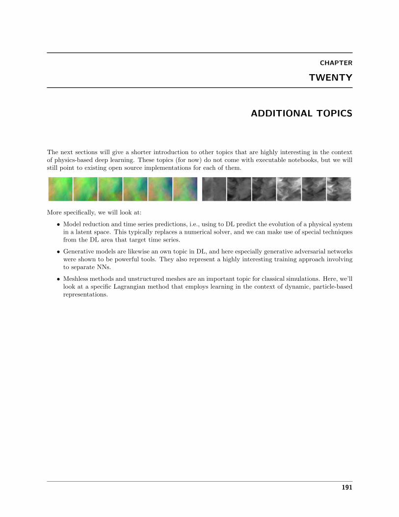
CHAPTER
TWENTY
ADDITIONAL TOPICS
The next sections will give a shorter introduction to other topics that are highly interesting in the contextof physics-based deep learning. These topics (for now) do not come with executable notebooks, but we willstill point to existing open source implementations for each of them.
More specifically, we will look at:
• Model reduction and time series predictions, i.e., using to DL predict the evolution of a physical systemin a latent space. This typically replaces a numerical solver, and we can make use of special techniquesfrom the DL area that target time series.
• Generative models are likewise an own topic in DL, and here especially generative adversarial networkswere shown to be powerful tools. They also represent a highly interesting training approach involvingto separate NNs.
• Meshless methods and unstructured meshes are an important topic for classical simulations. Here, we’lllook at a specific Lagrangian method that employs learning in the context of dynamic, particle-basedrepresentations.
191

Physics-based Deep Learning
192 Chapter 20. Additional Topics

CHAPTER
TWENTYONE
MODEL REDUCTION AND TIME SERIES
An inherent challenge for many practical PDE solvers is the large dimensionality of the resulting problems.Our model 𝒫 is typically discretized with 𝒪(𝑛3) samples for a 3 dimensional problem (with 𝑛 denoting thenumber of samples along one axis), and for time-dependent phenomena we additionally have a discretizationalong time. The latter typically scales in accordance to the spatial dimensions. This gives an overall samplescount on the order of 𝒪(𝑛4). Not surprisingly, the workload in these situations quickly explodes for larger 𝑛(and for all practical high-fidelity applications we want 𝑛 to be as large as possible).
One popular way to reduce the complexity is to map a spatial state of our system st ∈ R𝑛3
into a muchlower dimensional state ct ∈ R𝑚, with 𝑚 ≪ 𝑛3. Within this latent space, we estimate the evolution of oursystem by inferring a new state ct+1, which we then decode to obtain st+1. In order for this to work, it’scrucial that we can choose 𝑚 large enough that it captures all important structures in our solution manifold,and that the time prediction of ct+1 can be computed efficiently, such that we obtain a gain in performancedespite the additional encoding and decoding steps. In practice, the explosion in terms of unknowns forregular simulations (the 𝒪(𝑛3) above) coupled with a super-linear complexity for computing a new state stdirectly makes this approach very expensive, while working with the latent space points c very quickly paysoff for small 𝑚.
However, it’s crucial that encoder and decoder do a good job at reducing the dimensionality of the problem.This is a very good task for DL approaches. Furthermore, we then need a time evolution of the latent spacestates c, and for most practical model equations, we cannot find closed form solutions to evolve c. Hence,this likewise poses a very good problem for DL. To summarize, we’re facing two challenges: learning a goodspatial encoding and decoding, together with learning an accurate time evolution. Below, we will describean approach to solve this problem following Wiewel et al. [WBT19] & [WKA+20], which in turn employsthe encoder/decoder of Kim et al. [KAT+19].
Figure1: For time series predictions with ROMs, we encode the state of our system with an encoder 𝑓𝑒,predict the time evolution with 𝑓𝑡, and then decode the full spatial information with a decoder 𝑓𝑑.
193

Physics-based Deep Learning
21.1 Reduced order models
Reducing the dimension and complexity of computational models, often called reduced order modeling (ROM)or model reduction, is a classic topic in the computational field. Traditional techniques often employ tech-niques such as principal component analysis to arrive at a basis for a chosen space of solution. However, beinglinear by construction, these approaches have inherent limitations when representing complex, non-linear so-lution manifolds. In practice, all “interesting” solutions are highly non-linear, and hence DL has receiveda substantial amount of interest as a way to learn non-linear representations. Due to the non-linearity, DLrepresentations can potentially yield a high accuracy with fewer degrees of freedom in the reduced modelcompared to classic approaches.
The canonical NN for reduced models is an autoencoder. This denotes a network whose sole task is toreconstruct a given input 𝑥 while passing it through a bottleneck that is typically located in or near themiddle of the stack of layers of the NN. The data in the bottleneck then represents the compressed, latentspace representation c. The part of the network leading up to the bottleneck c is the encoder 𝑓𝑒, and thepart after it the decoder 𝑓𝑑. In combination, the learning task can be written as
arg min𝜃𝑒,𝜃𝑑|𝑓𝑑(𝑓𝑒(s; 𝜃𝑒); 𝜃𝑑) − s|22
with the encoder 𝑓𝑒 : R𝑛3 → R𝑚 with weights 𝜃𝑒, and the decoder 𝑓𝑑 : R𝑚 → R𝑛3
with weights 𝜃𝑑. Forthis learning objective we do not require any other data than the s, as these represent inputs as well as thereference outputs.
Autoencoder networks are typically realized as stacks of convolutional layers. While the details of theselayers can be chosen flexibly, a key property of all autoencoder architectures is that no connection betweenencoder and decoder part may exist. Hence, the network has to be separable for encoder and decoder. Thisis natural, as any connections (or information) shared between encoder and decoder would prevent using theencoder or decoder in a standalone manner. E.g., the decoder has to be able to decode a full state s purelyfrom a latent space point c.
21.1.1 Autoencoder variants
One popular variant of autoencoders is worth a mention here: the so-called variational autoencoders, orVAEs. These autoencoders follow the structure above, but additionally employ a loss term to shape thelatent space of c. Its goal is to let the latent space follow a known distribution. This makes it possible todraw samples in latent space without workarounds such as having to project samples into the latent space.
Typically we use a normal distribution as target, which makes the latent space an 𝑚 dimensional unit cube:each dimension should have a zero mean and unit standard deviation. This approach is especially useful ifthe decoder should be used as a generative model. E.g., we can then produce c samples directly, and decodethem to obtain full states. While this is very useful for applications such as constructing generative modelsfor faces or other types of natural images, it is less crucial in a simulation setting. Here we want to obtain alatent space that facilitates the temporal prediction, rather than being able to easily produce samples fromit.
194 Chapter 21. Model Reduction and Time Series
Physics-based Deep Learning
21.2 Time series
The goal of the temporal prediction is to compute a latent space state at time 𝑡 + 1 given one or moreprevious latent space states. The most straight-forward way to formulate the corresponding minimizationproblem is
arg min𝜃𝑝 |𝑓𝑝(c𝑡; 𝜃𝑝) − c𝑡+1|22where the prediction network is denoted by 𝑓𝑝 to distinguish it from encoder and decoder, above. Thisalready implies that we’re facing a recurrent task: any 𝑖𝑡ℎ step is the result of 𝑖 evaluations of 𝑓𝑝, i.e.
c𝑡+𝑖 = 𝑓(𝑖)𝑝 (c𝑡; 𝜃𝑝). As there is an inherent per-evaluation error, it is typically important to train this process
for more than a single step, such that the 𝑓𝑝 network “sees” the drift it produces in terms of the latent spacestates over time.
Koopman operators
In classical dynamical systems literature, a data-driven prediction of future states is typically formulatedin terms of the so-called Koopman operator, which usually takes the form of a matrix, i.e. uses a linearapproach.
Traditional works have focused on obtaining good Koopman operators that yield a high accuracy in combi-nation with a basis to span the space of solutions. In the approach outlined above the 𝑓𝑝 network can beseen as a non-linear Koopman operator.
In order for this approach to work, we either need an appropriate history of previous states to uniquelyidentify the right next state, or our network has to internally store the previous history of states it has seen.
For the former variant, the prediction network 𝑓𝑝 receives more than a single c𝑡. For the latter variant, wecan turn to algorithms from the subfield of recurrent neural networks (RNNs). A variety of architectureshave been proposed to encode and store temporal states of a system, the most popular ones being longshort-term memory (LSTM) networks, gated recurrent units (GRUs), or lately attention-based transformernetworks. No matter which variant is used, these approaches always work with fully-connected layers asthe latent space vectors do not exhibit any spatial structure, but typically represent a seemingly randomcollection of values. Due to the fully-connected layers, the prediction networks quickly grow in terms of theirparameter count, and thus require a relatively small latent-space dimension 𝑚. Luckily, this is in line withour main goals, as outlined at the top.
21.3 End-to-end training
In the formulation above we have clearly split the en- / decoding and the time prediction parts. However,in practice an end-to-end training of all networks involved in a certain task is usually preferable, as thenetworks can adjust their behavior in accordance with the other components involved in the task.
For the time prediction, we can formulate the objective in terms of s, and use en- and decoder in the timeprediction to compute the loss:
arg min𝜃𝑒,𝜃𝑝,𝜃𝑑|𝑓𝑑(𝑓𝑝(𝑓𝑒(s𝑡; 𝜃𝑒); 𝜃𝑝); 𝜃𝑑) − s𝑡+1|22
Ideally, this step is furthermore unrolled over time to stabilize the evolution over time. The resulting trainingwill be significantly more expensive, as more weights need to be trained at once, and a much larger numberof intermediate states needs to be processed. However, the increased cost typically pays off with a reducedoverall inference error.
To summarize, DL allows us to move from linear subspaces to non-linear manifolds, and provides a basis forperforming complex steps (such as time evolutions) in the resulting latent space.
21.2. Time series 195

Physics-based Deep Learning
Figure2: Several time frames of an example prediction from [WKA+20], which additionally couples thelearned time evolution with a numerically solved advection step. The learned prediction is shown at the top,the reference simulation at the bottom.
21.4 Source code
In order to make practical experiments in this area of deep learning, we can recommend this latent spacesimulation code, which realizes an end-to-end training for encoding and prediction. Alternatively, this learnedmodel reduction code focuses on the encoding and decoding aspects.
Both are available as open source and use a combination of TensorFlow and mantaflow as DL and fluidsimulation frameworks.
196 Chapter 21. Model Reduction and Time Series

CHAPTER
TWENTYTWO
GENERATIVE ADVERSARIAL NETWORKS
A fundamental problem in machine learning is to fully represent all possible states of a variable x underconsideration, i.e. to capture its full distribution. For this task, generative adversarial networks (GANs)were shown to be powerful tools in DL. They are important when the data has ambiguous solutions, andno differentiable physics model is available to disambiguate the data. In such a case a supervised learningwould yield an undesirable averaging that can be prevented with a GAN approach.
Figure1: GANs were shown to work well for tasks such as the inference of super-resolution solutions wherethe range of possible results can be highly ambiguous.
22.1 Maximum likelihood estimation
To train a GAN we have to briefly turn to classification problems. For these, the learning objective takes aslightly different form than the regression objective in equation (2) of Models and Equations: We now wantto maximize the likelihood of a learned representation 𝑓 that assigns a probability to an input x𝑖 given a setof weights 𝜃. This yields a maximization problem of the form
arg max𝜃Π𝑖𝑓(x𝑖; 𝜃), (1)
the classic maximum likelihood estimation (MLE). In practice, it is typically turned into a sum of negativelog likelihoods to give the learning objective
arg min𝜃 −∑𝑖
log𝑓(x𝑖; 𝜃).
There are quite a few equivalent viewpoints for this fundamental expression: e.g., it can be seen as minimizingthe KL-divergence between the empirical distribution as given by our training data set and the learned one.It likewise represents a maximization of the expectation as defined by the training data, i.e. E log𝑓(x𝑖; 𝜃).This in turn is the same as the classical cross-entropy loss for classification problems, i.e., a classifier with a
197

Physics-based Deep Learning
sigmoid as activation function.. The takeaway message here is that the wide-spread training via cross entropyis effectively a maximum likelihood estimation for probabilities over the inputs, as defined in equation (1).
22.2 Adversarial training
MLE is a crucial component for GANs: here we have a generator that is typically similar to a decodernetwork, e.g., the second half of an autoencoder from Model Reduction and Time Series. For regular GANs,the generator receives a random input vector, denoted with z, from which it should produce the desiredoutput.
However, instead of directly training the generator, we employ a second network that serves as loss for thegenerator. This second network is called discriminator, and it has a classification task: to distinguish thegenerated samples from “real” ones. The real ones are typically provided in the form of a training data set,samples of which will be denoted as x below.
For regular GANs training the classification task of the discriminator is typically formulated as
arg min𝜃𝑑− 1
2E log𝐷(y) − 1
2E log(1 −𝐷(𝐺(z))
which, as outlined above, is a standard binary cross-entropy training for the class of real samples y, andthe generated ones 𝐺(z). With the formulation above, the discriminator is trained to maximize the loss viaproducing an output of 1 for the real samples, and 0 for the generated ones.
The key for the generator loss is to employ the discriminator and produce samples that are classified as realby the discriminator:
arg min𝜃𝑔 − 1
2E log𝐷(𝐺(z))
Typically, this training is alternated, performing one step for 𝐷 and then one for 𝐺. Thus the 𝐷 networkis kept constant, and provides a gradient to “steer” 𝐺 in the right direction to produce samples that areindistinguishable from the real ones. As 𝐷 is likewise an NN, it is differentiable by construction, and canprovide the necessary gradients.
22.3 Regularization
Due to the coupled, alternating training, GAN training has a reputation of being finicky in practice. Insteadof a single, non-linear optimization problem, we now have two coupled ones, for which we need to finda fragile balance. (Otherwise we’ll get the dreaded mode-collapse problem: once one of the two network“collapses” to a trivial solution, the coupled training breaks down.)
To alleviate this problem, regularization is often crucial to achieve a stable training. In the simplest case,we can add an 𝐿1 regularizer w.r.t. reference data with a small coefficient for the generator 𝐺. Along thoselines, pre-training the generator in a supervised fashion can help to start with a stable state for 𝐺. (However,then 𝐷 usually also needs a certain amount of pre-training to keep the balance.)
198 Chapter 22. Generative Adversarial Networks

Physics-based Deep Learning
22.4 Conditional GANs
For physical problems the regular GANs which generate solutions from the randomized latent-space z aboveare not overly useful. Rather, we often have inputs such as parameters, boundary conditions or partialsolutions which should be used to infer an output. Such cases represent conditional GANs, which meansthat instead of 𝐺(z), we now have 𝐺(x), where x denotes the input data.
A good scenario for conditional GANs are super-resolution networks: These have the task to compute ahigh-resolution output given a sparse or low-resolution input solution.
22.5 Ambiguous solutions
One of the main advantages of GANs is that they can prevent an undesirable averaging for ambiguous data.E.g., consider the case of super-resolution: a low-resolution observation that serves as input typically has aninfinite number of possible high-resolution solutions that would fit the low-res input.
If a data set contains multiple such cases, and we employ supervised training, the network will reliably learnthe mean. This averaged solution usually is one that is clearly undesirable, and unlike any of the individualsolutions from which it was computed. This is the multi-modality problem, i.e. different modes existing asvalid equally valid solutions to a problem. For fluids, this can, e.g., happen when we’re facing bifurcations,as discussed in A Teaser Example.
The following image shows a clear example of how well GANs can circumvent this problem:
Figure2: A super-resolution example: a) input, b) supervised result, c) GAN result, d) high-resolutionreference.
22.6 Spatio-temporal super-resolution
Naturally, the GAN approach is not limited to spatial resolutions. Previous work has demonstrated that theconcept of learned self-supervision extends to space-time solutions, e.g., in the context of super-resolutionfor fluid simulations [XFCT18].
The following example compares the time derivatives of different solutions:
As can be seen, the GAN trained with spatio-temporal self-supervision (second from right) closely matchesthe reference solution on the far right. In this case the discriminator receives reference solutions over time (inthe form of triplets), such that it can learn to judge whether the temporal evolution of a generated solutionmatches that of the reference.
22.4. Conditional GANs 199
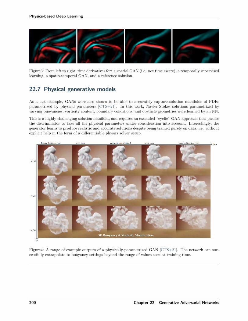
Physics-based Deep Learning
Figure3: From left to right, time derivatives for: a spatial GAN (i.e. not time aware), a temporally supervisedlearning, a spatio-temporal GAN, and a reference solution.
22.7 Physical generative models
As a last example, GANs were also shown to be able to accurately capture solution manifolds of PDEsparametrized by physical parameters [CTS+21]. In this work, Navier-Stokes solutions parametrized byvarying buoyancies, vorticity content, boundary conditions, and obstacle geometries were learned by an NN.
This is a highly challenging solution manifold, and requires an extended “cyclic” GAN approach that pushesthe discriminator to take all the physical parameters under consideration into account. Interestingly, thegenerator learns to produce realistic and accurate solutions despite being trained purely on data, i.e. withoutexplicit help in the form of a differentiable physics solver setup.
Figure4: A range of example outputs of a physically-parametrized GAN [CTS+21]. The network can suc-cessfully extrapolate to buoyancy settings beyond the range of values seen at training time.
200 Chapter 22. Generative Adversarial Networks

Physics-based Deep Learning
22.8 Discussion
GANs are a powerful learning tool. Note that the discriminator 𝐷 is really “just” a learned loss function:we can completely discard it at inference time, once the generator is fully trained. Hence it’s also not overlycrucial how much resources it needs.
However, despite being very powerful tools, it is (given the current state-of-the-art) questionable whetherGANs make sense when we have access to a reasonable PDE model. If we can discretize the model equationsand include them with a differentiable physics (DP) training (cf. Introduction to Differentiable Physics), thiswill most likely give better results than trying to approximate the PDE model with a discriminator. The DPtraining can yield similar benefits to GAN training: it yields a local gradient via the discretized simulator,and in this way prevents undesirable averaging across samples. Hence, combinations of DP training andGANs are also bound to not perform better than either of them in isolation.
That being said, GANs can nonetheless be attractive in situations where DP training is infeasible due toblack-box solvers without gradients
22.9 Source code
Due to the complexity of the training setup, we only refer to external open source implementations forpractical experiments with physical GANs. E.g., the spatio-temporal GAN from [XFCT18] is available athttps://github.com/thunil/tempoGAN.
It also includes several extensions for stabilization, such as 𝐿1 regularization, and generator-discriminatorbalancing.
22.8. Discussion 201

Physics-based Deep Learning
202 Chapter 22. Generative Adversarial Networks

CHAPTER
TWENTYTHREE
UNSTRUCTURED MESHES AND MESHLESS METHODS
For all computer-based methods we need to find a suitable discrete representation. While this is straight-forward for cases such as data consisting only of integers, it is more challenging for continuously changingquantities such as the temperature in a room. While the previous examples have focused on aspects beyonddiscretization (and used Cartesian grids as a placeholder), the following chapter will target scenarios wherelearning with dynamically changing and adaptive discretization has a benefit.
23.1 Types of computational meshes
Generally speaking, we can distinguish three types of computational meshes (or “grids”) with which dis-cretizations are typically performed:
• structured meshes: Structured meshes have a regular arrangement of the sample points, and animplicitly defined connectivity. In the simplest case it’s a dense Cartesian grid.
• unstructured meshes: On the other hand can have an arbitrary connectivity and arrangement. Theflexibility gained from this typically also leads to an increased computational cost.
• meshless or particle-based finally share arbitrary arrangements of the sample points with unstructuredmeshes, but in contrast implicitly define connectivity via neighborhoods, i.e. a suitable distance metric.
Structured meshes are currently very well supported within DL algorithms due to their similarity to imagedata, and hence they typically simplify implementations and allow for using stable, established DL compo-nents (especially regular convolutional layers). However, for target functions that exhibit an uneven mix ofsmooth and complex regions, the other two mesh types can have advantages.
Figure1: Lagrangian simulations of liquids: the sampling points move with the material, and undergo largechanges. In the top row timesteps of a learned simulation, in the bottom row the traditional SPH solver.
203

Physics-based Deep Learning
23.2 Unstructured meshes and graph neural networks
Within computational sciences the generation of improved mesh structures is a challenging and ongoingeffort. The numerous H-,C- and O-type meshes which were proposed with numerous variations over theyears for flows around airfoils are a good example.
Unstructured meshes offer the largest flexibility here on the meshing side, but of course need to be supportedby the simulator. Interestingly, unstructured meshes share many properties with graph neural networks(GNNs), which extend the classic ideas of DL on Cartesian grids to graph structures. Despite growingsupport, working with GNNs typically causes a fair amount of additional complexity in an implementation,and the arbitrary connectivities call for message-passing approaches between the nodes of a graph. Thismessage passing is usually realized using fully-connected layers, instead of convolutions.
Thus, in the following, we will focus on a particle-based method [UPTK19], which offers the same flexibilityin terms of spatial adaptivity as GNNs. These were previously employed for a very similar goal [SGGP+20],however, the method below enables a real convolution operator for learning the physical relationships.
23.3 Meshless and particle-based methods
Organizing connectivity explicitly is particularly challenging in dynamic cases, e.g., for Lagrangian represen-tations of moving materials where the connectivity quickly becomes obsolete over time. In such situations,methods that rely on flexible, re-computed connectivities are a good choice. Operations are then definedin terms of a spatial neighborhood around the sampling locations (also called “particles” or just “points”),and due to the lack of an explicit mesh-structure these methods are also known as “meshless” methods.Arguably, different unstructured, graph and meshless variants can typically be translated from one to theother, but nonetheless the rough distinction outlined above gives an indicator for how a method works.
In the following, we will discuss an example targeting splashing liquids as a particularly challenging case.For these simulations, the fluid material moves significantly and is often distributed very non-uniformly.
The general outline of a learned, particle-based simulation is similar to a DL method working on a Cartesiangrid: we store data such as the velocity at certain locations, and then repeatedly perform convolutions tocreate a latent space at each location. Each convolution reads in the latent space content within its supportand produces a result, which is activated with a suitable non-linear function such as ReLU. This is donemultiple times in parallel to produce a latent space vector, and the resulting latent space vectors at eachlocation serve as inputs for the next stage of convolutions. After expanding the size of the latent space overthe course of a few layers, it is contracted again to produce the desired result, e.g., an acceleration.
23.4 Continuous convolutions
A generic, discrete convolution operator to compute the convolution (𝑓 * 𝑔) between functions 𝑓 and 𝑔 hasthe form
(𝑓 * 𝑔)(x) =∑𝜏∈Ω
𝑓(x + 𝜏)𝑔(𝜏),
where 𝜏 denotes the offset vector, and Ω defines the support of the filter function (typically 𝑔).
We transfer this idea to particles and point clouds by evaluating a convolution on a set of 𝑖 locations x𝑖 ina radial neighborhood 𝒩 (x, 𝑅) around x. Here, 𝑅 denotes the radius within which the convolution shouldhave support. We define a continuous version of the convolution following [UPTK19]:
(𝑓 * 𝑔)(x) =∑𝑖
𝑓(x𝑖) 𝑔(Λ(x𝑖 − x)).
204 Chapter 23. Unstructured Meshes and Meshless Methods

Physics-based Deep Learning
Here, the mapping Λ plays a central role: it represents a mapping from the unit ball to the unit cube, whichallows us to use a simple grid to represent the unknowns in the convolution kernel. This greatly simplifiesthe construction and handling of the convolution kernel, and is illustrated in the following figure:
Figure2: The unit ball to unit cube mapping employed for the kernel function of the continuous convolution.
In a physical setting, e.g., the simulation of fluid dynamics, we can additionally introduce a radial weightingfunction, denoted as 𝑎 below to make sure the kernel has a smooth falloff. This yields
(𝑓 * 𝑔)(x) =1
𝑎𝒩
∑𝑖
𝑎(x𝑖,x) 𝑓(x𝑖) 𝑔(Λ(x𝑖 − x)),
where 𝑎𝒩 denotes a normalization factor 𝑎𝒩 =∑
𝑖∈𝒩 (x,𝑅) 𝑎(x𝑖,x). There’s is quite some flexibility for 𝑎,but below we’ll use the following weighting function
𝑎(x𝑖,x) =
⎧⎨⎩(
1 − ‖x𝑖−x‖22
𝑅2
)3
for ‖x𝑖 − x‖2 < 𝑅
0 else.
This ensures that the learned influence smoothly drops to zero for each of the individual convolutions.
For a lean architecture, a small fully-connected layer can be added for each convolution to process the contentof the destination particle itself. This makes it possible to use relatively small kernels with even sizes, e.g.,sizes of 43 [UPTK19].
23.5 Learning the dynamics of liquids
The architecture outlined above can then be trained with a collection of randomized reference data froma particle-based Navier-Stokes solver. The resulting network yields a good accuracy with a very small andefficient model. E.g., compared to GNN-based approaches the continuous convolution requires significantlyfewer weights and is faster to evaluate.
Interestingly, a particularly tough case for such a learned solver is a container of liquid that should come torest. If the training data is not specifically engineered to contain many such cases, the network receives onlya relatively small of such cases at training time. Moreover, a simulation typically takes many steps to cometo rest (many more than are unrolled for training). Hence the network is not explicitly trained to reproducesuch behavior.
Nonetheless, an interesting side-effect of having a trained NN for such a liquid simulation by constructionprovides a differentiable solver. Based on a pre-trained network, the learned solver then supports optimizationvia gradient descent, e.g., w.r.t. input parameters such as viscosity.
23.5. Learning the dynamics of liquids 205

Physics-based Deep Learning
Figure3: An example of a particle-based liquid spreading in a landscape scenario, simulated with learnedapproach using continuous convolutions [UPTK19].
23.6 Source code
For a practical implementation of the continuous convolutions, another important step is a fast collectionof neighboring particles for 𝒩 . An efficient example implementation can be found at https://github.com/intel-isl/DeepLagrangianFluids, together with training code for learning the dynamics of liquids, an exampleof which is shown in the figure above.
206 Chapter 23. Unstructured Meshes and Meshless Methods

Part VIII
End Matter
207


CHAPTER
TWENTYFOUR
OUTLOOK
Despite the lengthy discussions and numerous examples, we’ve really just barely scratched the surface re-garding the possibilities that arise in the context of physics-based deep learning.
Most importantly, the techniques that were explained in the previous chapter have an enormous potential toinfluence all computational methods of the next decades. As demonstrated many times in the code examples,there’s no magic involved, but deep learning gives us very powerful tools to represent and approximate non-linear functions. And deep learning by no means makes existing numerical methods deprecated. Rather, thetwo are an ideal combination.
A topic that we have not touched at all so far is, that - of course - in the end our goal is to improve humanunderstanding of our world. And here the view of neural networks as “black boxes” is clearly outdated. It issimply another numerical method that humans can employ, and the physical fields predicted by a networkare as interpretable as the outcome of a traditional simulation. Nonetheless, it is important to furtherimprove the tools for analyzing learned networks, and to extract condensed formulations of the patterns andregularities the networks have found in the solution manifolds.
24.1 Some specific directions
Beyond this long term outlook, there are many interesting and immediate steps. And while the examples withBurgers equation and Navier-Stokes solvers are clearly non-trivial, there’s a wide variety of other potentialPDE models that the techniques of this book can be applied to. To name just a few promising examplesfrom other fields:
• PDEs for chemical reactions often show complex behavior due to the interactions of multiple species.Here, and especially interesting direction is to train models that quickly learn to predict the evolutionof an experiment or machine, and adjust control knobs to stabilize it, i.e., an online control setting.
• Plasma simulations share a lot with vorticity-based formulations for fluids, but additionally intro-duce terms to handle electric and magnetic interactions within the material. Likewise, controllers forplasma fusion experiments and generators are an excellent topic with plenty of potential for DL withdifferentiable physics.
• Finally, weather and climate are crucial topics for humanity, and highly complex systems of fluid flowsinteracting with a multitude of phenomena on the surface of our planet. Accurately modeling all theseinteracting systems and predicting their long-term behavior shows a lot of promise to benefit from DLapproaches that can interface with numerical simulations.
209

Physics-based Deep Learning
24.2 Closing remarks
So overall, there’s lots of exciting research work left to do - the next years and decades definitely won’t beboring.
210 Chapter 24. Outlook
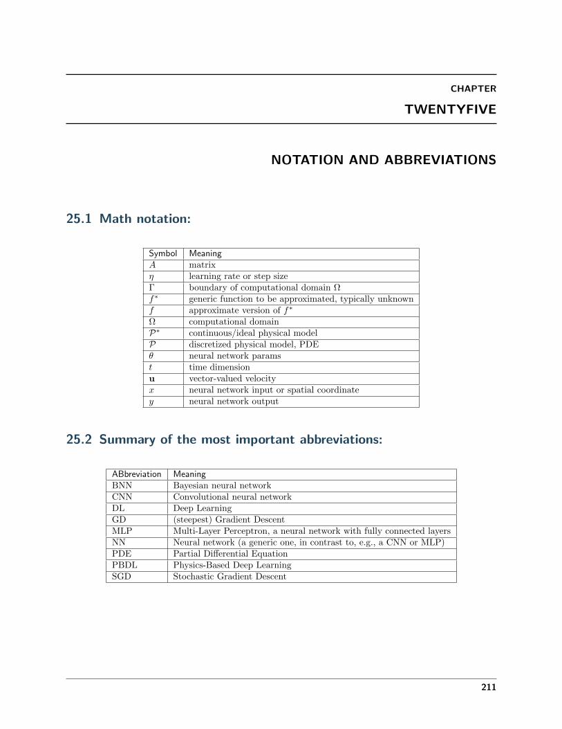
CHAPTER
TWENTYFIVE
NOTATION AND ABBREVIATIONS
25.1 Math notation:
Symbol Meaning𝐴 matrix𝜂 learning rate or step sizeΓ boundary of computational domain Ω𝑓* generic function to be approximated, typically unknown𝑓 approximate version of 𝑓*
Ω computational domain𝒫* continuous/ideal physical model𝒫 discretized physical model, PDE𝜃 neural network params𝑡 time dimensionu vector-valued velocity𝑥 neural network input or spatial coordinate𝑦 neural network output
25.2 Summary of the most important abbreviations:
ABbreviation MeaningBNN Bayesian neural networkCNN Convolutional neural networkDL Deep LearningGD (steepest) Gradient DescentMLP Multi-Layer Perceptron, a neural network with fully connected layersNN Neural network (a generic one, in contrast to, e.g., a CNN or MLP)PDE Partial Differential EquationPBDL Physics-Based Deep LearningSGD Stochastic Gradient Descent
211

Physics-based Deep Learning
212 Chapter 25. Notation and Abbreviations

BIBLIOGRAPHY
[AAC+19] Ilge Akkaya, Marcin Andrychowicz, Maciek Chociej, Mateusz Litwin, Bob McGrew, and others.Solving rubik’s cube with a robot hand. arXiv:1910.07113, 2019.
[CT21] Li-Wei Chen and Nils Thuerey. Towards high-accuracy deep learning inference of compressibleturbulent flows over aerofoils. In arXiv. 2021. URL: https://ge.in.tum.de/publications/.
[CTS+21] Mengyu Chu, Nils Thuerey, Hans-Peter Seidel, Christian Theobalt, and Rhaleb Zayer. LearningMeaningful Controls for Fluids. ACM Trans. Graph., 2021. URL: https://people.mpi-inf.mpg.de/∼mchu/gvv-den2vel/den2vel.html.
[Gol90] H Goldstine. A history of scientific computing. ACM, 1990.
[HKT19] Philipp Holl, Vladlen Koltun, and Nils Thuerey. Learning to control pdes with differentiablephysics. In International Conference on Learning Representations. 2019. URL: https://ge.in.tum.de/publications/2020-iclr-holl/.
[KAT+19] Byungsoo Kim, Vinicius C Azevedo, Nils Thuerey, Theodore Kim, Markus Gross, and BarbaraSolenthaler. Deep Fluids: A Generative Network for Parameterized Fluid Simulations. Comp.Grap. Forum, 38(2):12, 2019. URL: http://www.byungsoo.me/project/deep-fluids/.
[KB14] Diederik P Kingma and Jimmy Ba. Adam: a method for stochastic optimization.arXiv:1412.6980, 2014.
[KSA+21] Dmitrii Kochkov, Jamie A Smith, Ayya Alieva, Qing Wang, Michael P Brenner, and StephanHoyer. Machine learning-accelerated computational fluid dynamics. Proceedings of the NationalAcademy of Sciences, 2021.
[KUT20] Georg Kohl, Kiwon Um, and Nils Thuerey. Learning similarity metrics for numerical simulations.International Conference on Machine Learning, 2020. URL: https://ge.in.tum.de/publications/2020-lsim-kohl/.
[KSH12] Alex Krizhevsky, Ilya Sutskever, and Geoffrey E Hinton. Imagenet classification with deep con-volutional neural networks. In Advances in Neural Information Processing Systems. 2012.
[MLA+19] Rajesh Maingi, Arnold Lumsdaine, Jean Paul Allain, Luis Chacon, SA Gourlay, and others.Summary of the fesac transformative enabling capabilities panel report. Fusion Science andTechnology, 75(3):167-177, 2019.
[OMalleyBK+16] Peter JJ O’Malley, Ryan Babbush, Ian D Kivlichan, Jonathan Romero, Jarrod R McClean,Rami Barends, Julian Kelly, Pedram Roushan, Andrew Tranter, Nan Ding, and others. Scalablequantum simulation of molecular energies. Physical Review X, 6(3):031007, 2016.
[Qur19] Mohammed Al Quraishi. Alphafold at casp13. Bioinformatics, 35(22):4862-4865, 2019.
[RWC+19] Alec Radford, Jeffrey Wu, Rewon Child, David Luan, Dario Amodei, and Ilya Sutskever. Lan-guage models are unsupervised multitask learners. OpenAI blog, 1(8):9, 2019.
213

Physics-based Deep Learning
[RK18] Maziar Raissi and George Em Karniadakis. Hidden physics models: machine learning of non-linear partial differential equations. Journal of Computational Physics, 357:125-141, 2018.
[SGGP+20] Alvaro Sanchez-Gonzalez, Jonathan Godwin, Tobias Pfaff, Rex Ying, Jure Leskovec, and PeterBattaglia. Learning to simulate complex physics with graph networks. In International Confer-ence on Machine Learning, 8459-8468. 2020.
[SML+15] John Schulman, Philipp Moritz, Sergey Levine, Michael Jordan, and Pieter Abbeel. High-dimensional continuous control using generalized advantage estimation. arXiv:1506.02438, 2015.
[SWD+17] John Schulman, Filip Wolski, Prafulla Dhariwal, Alec Radford, and Oleg Klimov. Proximalpolicy optimization algorithms. arXiv:1707.06347, 2017.
[SSS+17] David Silver, Julian Schrittwieser, Karen Simonyan, Ioannis Antonoglou, Aja Huang, and others.Mastering the game of Go without human knowledge. Nature, 2017.
[Sto14] Thomas Stocker. Climate change 2013: the physical science basis: Working Group I contributionto the Fifth assessment report of the Intergovernmental Panel on Climate Change. Cambridgeuniversity press, 2014.
[SB18] Richard S Sutton and Andrew G Barto. Reinforcement learning: An introduction. MIT press,2018.
[TWPH20] Nils Thuerey, Konstantin Weissenow, Lukas Prantl, and Xiangyu Hu. Deep learning methods forreynolds-averaged navier-stokes simulations of airfoil flows. AIAA Journal, 58(1):25-36, 2020.URL: https://ge.in.tum.de/publications/2018-deep-flow-pred/.
[TSSP17] Jonathan Tompson, Kristofer Schlachter, Pablo Sprechmann, and Ken Perlin. Accelerating eule-rian fluid simulation with convolutional networks. In Proceedings of Machine Learning Research,3424-3433. 2017.
[UBH+20] Kiwon Um, Robert Brand, Philipp Holl, Raymond Fei, and Nils Thuerey. Solver-in-the-loop: learning from differentiable physics to interact with iterative pde-solvers. Advancesin Neural Information Processing Systems, 2020. URL: https://ge.in.tum.de/publications/2020-um-solver-in-the-loop/.
[UPTK19] Benjamin Ummenhofer, Lukas Prantl, Nils Thuerey, and Vladlen Koltun. Lagrangian fluid sim-ulation with continuous convolutions. In International Conference on Learning Representations.2019. URL: https://ge.in.tum.de/publications/2020-ummenhofer-iclr/.
[WBT19] Steffen Wiewel, Moritz Becher, and Nils Thuerey. Latent-space Physics: Towards Learning theTemporal Evolution of Fluid Flow. Comp. Grap. Forum, 38(2):12, 2019. URL: https://ge.in.tum.de/publications/latent-space-physics/.
[WKA+20] Steffen Wiewel, Byungsoo Kim, Vinicius C Azevedo, Barbara Solenthaler, and Nils Thuerey.Latent space subdivision: stable and controllable time predictions for fluid flow. Symposium onComputer Animation, 2020. URL: https://ge.in.tum.de/publications/2020-lssubdiv-wiewel/.
[XFCT18] You Xie, Erik Franz, Mengyu Chu, and Nils Thuerey. tempoGAN: A Temporally Coherent,Volumetric GAN for Super-resolution Fluid Flow. ACM Trans. Graph., 2018. URL: https://ge.in.tum.de/publications/tempogan/.
214 Bibliography