physics i : oscillations and waves prof. s. bharadwaj...

Physics I : Oscillations and Waves

Prof. S. Bharadwaj

Department of Physics & Meteorology

Indian Institute of Technology, Kharagpur

Lecture No – 15

Interference – II

Good morning. In the last class, we had started discussing interference and we had taken

up the Young’s double slit experiment for discussion. And then I was telling you about a

different way in which we can analyze the same Young’s double slit experiment. So, let

we recapitulate the thing that I was telling you at the end of the last lecture.

(Refer Slide Time: 01:34)

So, the Young’s double slit experiment can be realized in the following manner, I have a

plane wave incident over here the plane wave is incident on 2 prisms 2 very thin prisms

placed with their bases aligned. So, the base of these 2 thin prisms are struked together

and the 2 prisms are exactly opposite each other let me, just show over here this device is

called the biprism. So, when this plane wave passes through the biprism the upper prism

produces a wave, which is traveling downwards along with the wave vector k2 the lower

prism produces a wave which is traveling upwards with a wave vector k1.

So, the using the bi prism from a single source let us say, you had a distance source over

here a distant point source over somewhere, far away in this direction then by the time

the wave reaches the biprism you would have a plane wave. The biprism what the prism

does is from a single source from a single single plane wave it produces 2 plane waves.

So, this is a exactly like the Young’s double slit experiment it is a realization of the

Young’s double slit experiment you have produce 2 waves from the same source these 2

waves are incident on a screen over here and you get you will get an interference pattern

on the screen over here because of the superposition of these 2 waves. And in the last

lecture you are analyzing the what happens when you superpose these 2 waves.


So, we had started the analysis as follows: we first consider the point A so, we first had a

point A. So, we have a point A where the phases of the 2 waves are identical. So, let us

say, that the point A over here is such that both waves arrive at exactly the same phase at

this point A on the screen. So, this is the screen this is the wave vector of the wave which

is travelling upwards 1 of the waves k1 this is the wave vector of the other wave k2.

They both make an angle theta by 2 with respect to the normal to the screen.

Now we first identify the point A where both the waves arrive at the same phase. If both

waves arrive at the same phase then the intensity the electric field of these 2 waves are

going to oscillate in exactly the same phase. So, the they are going to add up and you’re

going to have a maxima in the intensity at the point A on the screen over here.

So, at this point both the electric field of both vectors E1 and E2 have the same

magnitude E and a same phase e I to the power phi A. We then ask the question what

happens if I move away from this point where I have a maxima to the another point B. If

you move away from this point A to a point B the phase of the first wave is going to

change by an amount, which is minus k1 dot r where k1 is the wave vector of the first

wave. So, for the first wave at the point B the phase phi 1 at the point B phi 1 is the

phase of the first wave at the point B is going to be the phase of the point A minus k1 dot

delta r, where delta r is the displacement between the point A and B.

Similarly, for the second wave the phase of the second wave at point B is going to be phi

A minus k2 dot delta r. And since k1 the and the k2 are the 2 different wave vectors the

difference arises because the 2 waves are travelling in different directions. Because k1

and k2 are different the phase of the 2 waves at this point B are going to be different. So,

phi 1 and phi 2 at the point B are going to be different.

So, there is going to be a phase difference between the 2 waves at the point B and you

can calculate the phase difference, the phase difference at the point B phi 2 B minus phi

1 B this phase difference you can calculate this by just subtracting this from this which

gives us minus k2 minus k2 minus k1. So, the difference of the 2 wave vectors dot delta

r. So, the phase difference between the 2 waves at the point B is k2 minus k1 the

difference in the wave vectors dot delta r and over all minus sign.

So, the point to note here is that: at the point A at A the 2 waves are at the same phase.

So, they you have a maxima in the intensity as you move away from A the phase of the

first wave changes by a certain amount, the phase of the second wave changes by a

different amount. So, as you move away from the point A the 2 waves come with the

phase difference and if the 2 waves have a phase difference then the intensity is no

longer at the maxima you have the intensity will go down.

So, as you move away from the point where you have a maxima the intensity is going to

go down and then you are going to get an intensity pattern on the screen this intensity

pattern is the is the interference pattern that we are interested in.


Now, let us ask the question where will I have a maxima. So, we started off a maxima at

the point A we started off at a maxima at the point A the question is at what

displacement will I have a maxima again. Now, at the point A the 2 waves had exactly

the same phase as I move away from A the phases of the 2 waves start to differ. Now,

you will again reach a maxima when the difference is a is a multiple of 2 pi and you will

have a minima when the difference is an odd multiple of pi when the difference between

the 2 waves k1 and k2.

So, this wave arrives at 1 phase this wave arrives at a difference phase when I move

away from the point A and as I move away the phase difference increases when the

phase difference becomes equal to pi then the oscillations of the electric field of this

wave and the oscillations of the electric at of this wave exactly cancel out and I have a

minima. So, the condition for minima is that the phase difference between the 2 waves

should be equal to pi or it could be 3 pi 5 pi sum odd multiple of pi.

So, this expression over here tells us at what displacement from the point A, I will have a

minima in the intensity. Now, once I cross the minima then keep on moving further out

the phase difference will increase further and then if the phase difference becomes an

even multiple of pi that is 2 pi 4 pi etcetera. The 2 electric fields again oscillating phase

and I have a maxima. So, I have a maxima minima and then intermediate values

depending on weather this and condition is satisfied or this condition is satisfied or if it is

somewhere in between then I will have some intensity in between.

So, this tells us the condition for the maximum intensity and the minimum intensity on

the screen. Now let us so, this depends as you can see this depends on 2 things it depends

on the direction of the 2 wave vector it also depends on the displacement delta r on the

screen. So, let us now take up particular situation which is relatively simple to analyze.


So, we will take up a particular case, the particular case that we’re going to discuss. So,

we will now take up a particular situation the particular situation that, we are going to

discuss we have 2 waves which are incident on the screen. And the 2 waves are incident

at an angle which is very small to the normal now a point which I should mention over

here I have shown you. So, from the analysis that we have done until now what we see is

that we will get some variation in the intensity pattern on the screen there will be

maximas and there will be minimas and there will be points in between where the

intensity is going to have intermediate values.

Now, we have not seen, we have not analyzed as yet what these patterns are going to

look like now, it is quiet straight forward to realize that if the 2 wave vectors and the

normal to the plane, normal to the screen on which the 2 waves are incident. So, there are

3 vectors involved the 2 wave vectors and the normal to the screen on which the wave is

incident if these three vectors are coplanar the 2 wave vectors and the normal to the

screen if these are coplanar, you will then get straight line fringes.

So, this the situation that we are going to consider now and let me show you that we need

will get straight line fringes in this particular case.


So, this is the particular case that we are going to take up we have a screen over here the

screen is aligned perpendicular to the x axis as you can see over here. So, you have a

screen the screen is aligned perpendicular to the x axis there are 2 waves incident on the

screen the wave, the first wave has a wave vector k1 it makes an angle theta by 2 with

the x axis and it is in the x y plane.

So, this is the x y plane which I am showing you here the first wave is incident at an

angle theta by 2 to the to the x direction which is normal to the screen over here. And the

second wave k2 is also incident at an angle theta by 2 it is travelling downwards. So,

both these waves are in the x y plane and they both make an angle theta by 2 with respect

to the x axis. So, the normal to the surface is the x axis and both these waves are in the x

y plane. So, all three of them are coplanar.

Now, let us first write down the wave vector k1 corresponding to the wave travelling

upwards. So, corresponding to this wave over here corresponding to the wave traveling

upwards which is the wave over here corresponding to this wave.

Let we first write down the wave vector. So, the wave vector of the wave travelling

upwards is what is given over here k1. So, k1 is 2 pi by lambda into the unit vector of the

direction in which the wave is propagating 2 pi by lambda is the wave number of this

wave. And the unit vector along which the wave is propagating is cos theta by 2 into I

this angle over here with respect to the x axis is theta by 2.

So, this unit vector has a component cos theta by 2 in the x direction it has a component

sin theta by 2 in the y direction. So, it gives us the unit vector cos theta by 2 into I plus

sin theta by 2 into j further we are going to assume that theta is very small. So, both the

waves are nearly normally incident, but not exactly so as a consequence there is a small

angle theta 2 between this wave vector on the x axis. If you assume that this small then

the cosine can be replaced by 1 the sin can be replaced by theta by 2.

So, the wave vector k1 is approximately equal to 2 pi by lambda I plus theta by 2 into j.

Let us next, look at the wave which is travelling downwards. So, let us look at this k2 the

only difference between k1 and k2 is that the y component will have a negative sign the

x component will be exactly the same which you can see from here. This is traveling

along the plus x direction. So, is this the only difference is this is traveling downwards

negative y whereas, this is travelling upwards positive y.

So, k2 the wave vector k2 is approximately 2 pi by lambda I minus theta by 2 into j

where we have assumed that theta is very small. Now, the expression for the phase

difference is k2 minus k1 dot delta r we would like to calculate the phase difference

between 2 points A and B. And this is given by k2 minus k1 dot delta r there is a minus

sign, but that does not matter. Where delta r refers the delta r here refers to possible

displacements on the screen.

Now, recollect that the screen is perpendicular to the x axis. So, the screen is in the y z

plane. So, any arbitrary displacement on the screen can be written will have a component

along the y axis. So, delta r on the screen can be written as delta y into j and the

displacement will can also have a component along the z axis. So, delta z into k. So, any

arbitrary displacement on the screen which is in the y z plane can be expressed in this

form it can have only a y component and a z component.

So, we use this and this we use all 3 of them in the expression for the phase difference k2

minus k1 dot delta r when you do k2 minus k 1. So, k2 minus k1 this term I the I

component exactly cancels out and what you are left with is essentially theta 2 pi by

lambda into theta j. So, k2 minus k1 is 2 pi by lambda into theta j with a minus sign. So,

there will be a minus sign, but we are not really concerned about the sign. So, we are not

written it over here. So, k2 minus k1 let me write it down over here or I can do it here.



So, k2 minus k1 the difference in the 2 wave vectors is 2 pi by lambda theta into j and

when you do a dot product with delta r which are possible displacements on the screen it

fix up only the y component there is no z component in k2 minus k1. So, that does not

contribute. So, the phase difference between any 2 points on the screen any point A and

another point B is given by this expression over here 2 pi theta by lambda into delta y.

And if A is a maxima if A is a maxima if you ask the question where will I have a

maxima again then the phase difference should be an even multiple of 2 pi the phase

difference we are assuming is 0 over here. So, I have a maxima in the intensity the phase

difference should be an even multiple of 2 pi for another maxima. So, it should satisfy

the phase difference should satisfy the condition that it should be equal to 2 into n into

pi. Where n could be any integer 0 plus minus 1 plus minus 2 etcetera and the plus minus

sign tell us while we did not bother about the negative sign.


So, what we see is that: you will have maximas in the y direction. So, the intensity first

point is that the phase changes only when you move along the y direction and you will

have maximas at a spacing at an equal interval in the y direction and.

(Refer Slide Time: 20:44min)

The spacing between the maxiams is lambda by theta


You can easily see that from here. So, if you just these factors of 2 pi will cancel out and

you will get maxiams at a spacing along the y direction at a spacing of delta y which is

equal to lambda by theta.


So, along the y direction you are going to get change in intensity you will have bright

dark bright, dark bright dark this and these fringes are going to extend they are going to

be lines along the z direction. And the spacing between the 2 bright fringes or the 2 dark

fringes is going to be lambda by theta.


So, these fringes which you get over here are going to be aligned parallel to the z

direction the intensity changes only along the y axis. So, the fringes are going to be

aligned parallel to be z direction you are going to get straight line fringes. And the

spacing between 2 bright fringes is delta y is equal to lambda by theta. Similarly, the

spacing between 2 dark fringes is also delta y is equal to lambda by theta


The resultant pattern is a pattern of bright, dark, bright, dark so, forth which is going to

extend all through the screen. Now, in the previous lecture and in this lecture we

essentially considered the Young’s double slit experiment. Let me just remind you what

the Young’s double slit experiment was: in the Young’s double slit experiment


We had A point source and the point source was incident on 2 slits. So, the point source

was incident on 2 slits each slit now acts like a source. So, if you want to calculate the

intensity at a point P here you have to calculate the wave that comes from this slit and

the wave that comes from this slit these 2 waves will be superposed here. They will be

superposed with a path difference which will introduce a phase difference and it is this

phase difference which causes the intensity to vary at different points over here you will

get pattern of dark, bright, dark, bright lines which are the fringes.

The same thing can also be realize these 2 sources can also be realized by sending a

wave on to a biprism the biprism produces 2 waves travelling at an angle with respect to

each other. When these are incident on a screen you will get a pattern of fringes bright

dark, bright dark and we have calculate the fringe spacing you can convince yourself you

should actually check that this situation and this situation are essentially the same they

are exactly the same situation.

Let us now, take up a problem. So, the problem we are going to take is as follows let me

take up a problem over here where we can apply some of these things.


So, the problem has to do with something called billet’s lens. So, the situation that we

wish to analyze is as follows, we have a lens over here the lens has a diameter of 25

centimeters which is not very important in the particular problem. We are going to

discuss the lens has a diameter of a 30 centimeters and it has focal length of 25

centimeters.

Now, what is done is that a part of this lens from the center, which is 1 millimeter wide.

So, part of the lens which is 1 millimeter wide from the center a part of a lens 1

millimeter wide is cut out. So, this part of lens is cut out. And the 2 remaining parts of

the bits of lens are again joined. So, what we have is something which looks like this

these are now joined. So, 1 millimeter from the center is cut out and these 2 parts of lens

are joined. Now, this whole apparatus is illuminated from a point source which is placed

at the focus.

So, there is a point source which is placed at the focus of this lens. So, this is the distance

f. So, the point source is placed over here and then you put a screen at a distance of 50

centimeters. So, there is a screen at a distance of 50 centimeters over here. And you have

been asked to calculate the fringe spacing on the screen over there. So, let us try to

understand how to go about and solve this problem. So, first question that we have to

address is why in the why do you expect to see any fringes on the screen at all you will

realize that this situation over here is very similar to the biprism that we have been

considering.


So, let me tell you how to solve this problem the first point which you should note is as

follows, if I have a lens over here and I put a source on the focal plane. So, this is the

focal plane this distance is the focal length if I put a source at the focus this produces a

wave which. So, this, this is a focus of the lens. So, this emits this is a point source. So, it

emits a spherical wave the property of a lens is that if this point source is placed at the

focus the wave that comes out is a plane wave and the plane wave is aligned with the

axis of the lens, if the source is at the focus.

So, if the source is aligned with the axis of the lens the wave that comes out is also

aligned with the axis of the lens. Now, for the same lens if I move the source up a little

bit. So, for the same lens if I move the source up a little bit. So, the source has been

moved up a little bit what happens I am sure all of us know this from geometrical optics

that the that the wave that comes out. So, the wave that comes is now no longer parallel

to the axis of the lens it comes out at an angle.

So, the wave that comes out is now at an angle if I shift the source up the wave comes

out at an angle downwards. If I shift the source down the wave will come out upwards

this is the property of a lens on the focal plane if I move the source up or down the wave

the for all of these situations. The light that comes out will be a plane wave the only

difference is that you can change the direction by moving the source up and down in the

focal plane and if you move it up an angle theta.

If you move the source up an angle theta then this is also going to move down an angle

theta and if the distance that you move this up is delta x then the angle is approximately

delta x by the focal length f. So, this is going to be the angle by which the wave that

comes out is going be going to make with the axis with the symmetry axis of the lens.

So, this is going to be the angle theta which the wave is going to make with the

symmetry axis of the lens. Now in the problem which we have been given.


The lens so, this is your lens and this is your source the lens is cut over here. So, the lens

is cut by an amount delta x and the upper part of lens is shifted down and the lower part

of the lens is shifted up. This is equivalent to shifting the source up or down by an

amount delta x by 2. So, for the upper lens, upper part of the lens when I shift it down

this is equivalent to shifting the source up by an amount delta x by 2.

So, the upper part of the lens is going to produce a wave that comes out in this direction

and this wave if I call this angle theta by 2 then theta by 2 is equal to delta x by 2 divided

by f. Similarly, the lower part of the lens as far as this is concerned and I move the lower

part I cut out this portion and move the lower part up this is equivalent to shifting the

source down by an amount by the exactly the same amount. So, the lower part of the of

the lens is going to produce a wave travelling in this direction.


So, let me draw this in a different picture the billet’s lens for a source placed in the center

the upper part of the billet’s lens is going to produce a wave travelling downwards and

the lower part is going produce a wave traveling upwards. And they each make an angle

theta by 2 which is delta x by 2 divided by f with respect to the axis of the lens. Now,

this is precisely the situation that we have been analyzing.

So, what we see is that if we put a screen over here on this screen there going to be 2

waves. These 2 waves are directly to be coherent because they originate from the same

source on the screen over here, you will have 2 waves and 1 wave is going to arrive at an

angle making an angle theta by 2 with the normal direction the another is also going to

arrive making an angle theta by 2. But these 2 1 is going upwards 1 is going downwards

and what you are going to get is a fringe pattern with a spacing delta y is equal to lambda

by theta.

So, if you doing this whole experiment with yellow light or with a let us say, which has

got yellow light which has got something around say light which has got a wavelength of

500 nanometers. This is lambda and theta we know that theta is delta x by f from here.

So, this tells us the value of theta and we can use this to calculate the spacing of the

fringes on the screen right. So, you can calculate this for the values which have been

given to you 1 millimeter is the is delta x f is a 25 centimeters.

So, for these numbers you can putting these numbers calculate theta lambda is given. So,

you can get the fringe spacing on the screen over here. So, this is 1 particular situation

where we can apply some of the things that we have learnt in the in today’s class


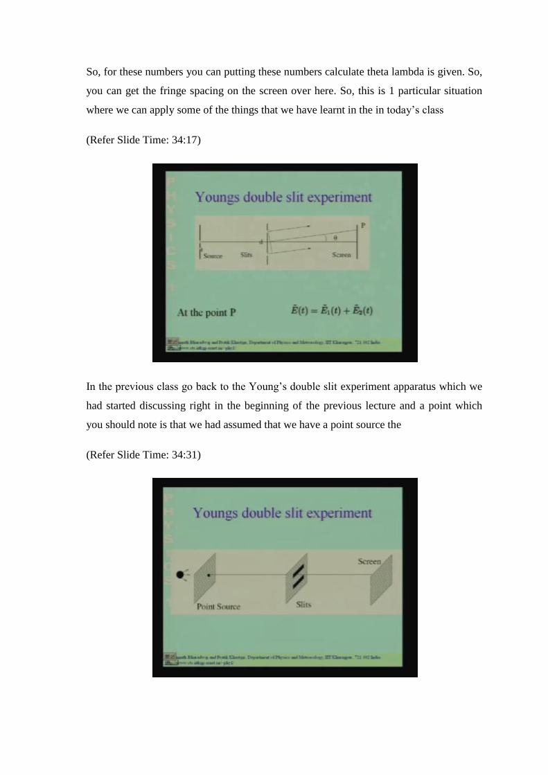
In the previous class go back to the Young’s double slit experiment apparatus which we

had started discussing right in the beginning of the previous lecture and a point which

you should note is that we had assumed that we have a point source the


And the point source was achieved by taking a, a screen over here which is illuminated

by a ball or something like that and making a very small hole on this screen. So, that

light comes out from only this very small aperture or pin hole you may say. And the

reason why this was done is we shall be discussing it now.


But in the less in the remaining part of the today’s lecture we are going to discuss what

happens when you make the slit when you take into account the finite angular extent of

the source. To make matters clear, what we are talking about if you do Michelson’s if

you do a Young double slit experiment with a distant star as a source. Now, a distant star

is has practically has the angular extent of the distant star for distant star cannot be

measured it is a point source it is as good a point source as you can get.

So, the light that comes from there is a single plane wave and the analysis that we have

done until now would be a precisely valid in such a situation. Let us consider, a situation

where you have a source which has a finite angular extent for example, the sun

sometimes at angle of around half a degree. So, if you were to do Young’s double slit

experiment using the sun as the source. So, sun light falls on the 2 slits how would that

effect my fringe pattern. It the question that we are asking is something equivalent to

that.


So, let me draw a picture over here explaining the situation that we are going deal with

now. So, the situation that we have now is like this, we have a source and then the this is

a line through the center of the source. The source is aligned with the slit. So, the slit this

is the this these are the 2 slits and then we have the screen over here. And the 2 slits are

at a separation of a distance d. So, this separation between the 2 slits is d and these

distances from the source to the slits and the slit to the screen is quite large that is the

assumption that we are making.

Now, we are going to take into account the final the finite angular extent of the source.

So, we are going assume that the source subtends an angle alpha. So, it extends from

minus alpha by 2 to plus alpha by 2 the source subtends an angle alpha at the slits. So,

this angle subtended by the source at the slits this angle is alpha. Now, we have to make

at this point we have to make a certain assumption about the nature of the source. So, for

example.


Let us again go back to the sun think of your sun as the source. So, this, the source the

source has got a finite angular extent now this large finite angular extent source I can

think of an individual point sources, I can think of as a collection of many point sources I

am only drawing a few of them now the question is as follows each of these point

sources is going to emit a wave. Each of these point sources is going to be a source for a

wave and when you do interference you have to superpose waves.

Now, the question is as follows will the wave from this particular point source and let us

say this particular point source or the waves from these 2 different point sources or the

source going to interfere do these interfere. Now, we it is our common experience that

that these the waves which are emitted from such sources do not interfere such these

sources are said to be incoherent.

So, we are going to assume that, different points on this extended source are incoherent

sources what we mean by that is, that the radiation from different points on my extended

source do not interfere the waves from these different points do not interfere with 1

another. For example if we have the sun the radiation from different points on the sun

will not interfere with 1 another. And such a assumption is quite reasonable because

there is no correlation between the radiations that comes from 1 point on the surface of

the sun and the other.

So, there no reason why we expect them to interfere with 1 another such sources are said

to be incoherent. So, we are going to assume that different points on sources are

incoherent sources.


So, here coming back to the situation that, we are analyzing we are going assume that

each point on this source which has a finite extent each point is acting like an incoherent

source. And when I have 2 incoherent sources I do not need, there is no need to

superpose the waves from these sources because the waves do not interfere that is what

we mean by incoherent 2 sources are said to be incoherent if the waves emitted by them

do not interfere we will go into what we mean by coherence and incoherence in a little

more detail in a later lecture.

But, for the time being we are going to assume that different points on this extended

source are incoherent what we mean by that is that the waves emitted from these

different points are not going to interfere with 1 another. So, when we want to find the

resultant intensity on the screen I can add up the intensity pattern from each of these

sources and there is no need to add up the waves from each of these sources. I can take

up single source calculate the intensity pattern take the next source calculate the intensity

pattern and so, forth.

And add up all the intensities to get the resultant intensity here this is because we have

assumed that the different sources over here are incoherent. So, let us do this calculation.

So, let us do this calculation. So, we will a take a point on the source which is at an angle

beta. So, the we will take a point on the source which is at an angle beta. So, this is at an

angle beta. Let us, take a point on the screen which is at an angle theta and let us

calculate the intensity produced by the source at a point beta on.

So, there is a point source on the point beta over here which is a part of my extended

source we would like to calculate the intensity produced by this point source on the

screen over here at an angle theta with respect to the center of the slits with respect to the

slits to do this we have to calculate the phase difference. So, we have to calculate the

phase difference of the wave. So, there will be wave emitted from here the wave will go

to slit 1 and the wave will go to slit 2.

So, the wave from the point at an angle beta will reach this point through either slit 1 or

slit 2 actually through both of them and we have to superpose both of these. So, not

through either of them, but through both of them and we have to superpose the wave that

reaches this point through slit 1 with the wave that reaches this point through slit 2 these

2 waves will arrive at different phases. So, what we have to calculate first is the phase

difference between these between the wave that goes from this point to this point through

this slit and this slit.

So, let me draw the picture in a different way and the phase difference should be clear.


So, this is the these are the 2 slits, this we will call this slit 1, we will call this slit 2 and

the wave arrives at an angle beta. So, there is a path difference over here. And the waves

goes out at an angle theta and there is. So, there is a path difference over here the path

difference over here is 2 d d is the separation between the 2 slits. So, the path difference

over here is 2 d sin beta and the path difference over here is 2 d sin theta. So, the total

path difference is 2 d sin beta plus sin theta.

And the phase difference to calculate the phase difference not 2 d, d sin theta this is d sin

beta and this is d sin theta this angle is beta this angle is theta. So, the path total path

difference between the wave that goes through slit 1 and the wave that goes through slit

2 is d din beta plus theta to calculate the phase difference you have to multiply this with

2 pi by lambda. So, this gives us phi 2 minus phi 1 and for small values of theta and beta.


The phase difference is 2 pi by lambda d theta plus beta and if you use this in the

expression for the intensity which let me, show you again. So, this is the expression for

the intensity if you use this in the expression for intensity.



And put in the fact that the I1 I2 are the same then you will get I theta beta is equal to 2 I

1 plus cos 2 pi by lambda d theta plus beta right. So, this is the expression that we want

what does this expression tell us let we again remind you of this.


We are dealing with an extended source and we have focused our attention on a

particular point on the extended source the particular point on the extended source is at

an angle beta. And we want to calculate the intensity on the screen at an angle theta due

to this point at an angle beta on the source


And we just did the calculation this intensity is on the screen at an angle theta due to a

source at an angle beta is given by the expression over here provided theta and beta are

small.


Now, if you wish to calculate the intensity at this point due to the entire source, the entire

source spans from minus alpha by 2, 2 alpha by 2 spans a total angle alpha. So, the total

intensity at this point can be calculated.


So, the intensity at the point over there can be calculate by adding up.


This can be calculated by adding up the intensity contributions from all of these points

remember we have assumed that each point over here is an incoherent source. So, we

have to add up the intensity contributions from all of these points to get the resultant

intensity over here.


So, this can be calculated as follows 1 by I am dividing by the total angle alpha just for

convenience it does not make any difference from minus alpha by 2 to plus alpha by 2 I

theta comma beta d beta. So, what we have done is: we have calculated the intensity

produced by a single point on the source and then we add up the contribution from all the

points on the source.

So, beta refers to the angle of the point on the source and beta has to be integrated from

minus alpha by 2 to alpha by 2 to get the total intensity on the at any point on the screen

which is what we have over here. So, we have to do this very simple integral over here

let me do this integral. So, when I integrate this constant term it gives me the same factor

of 2 I be that is why I have divided by alpha so, as to make things easy. So, the constant

term gives me a factor. So, let me write down the resultant of this integral the constant

term gives me a factor which is just the same thing itself 2 I.


So, I have I theta is equal to 2 I that is the contribution from the.


From the constant term over here, now when I do the beta integral over here this will

give me sin and I will have a factor of 1 by 2 pi d lambda.


So, I can write it like this 1 plus lambda by 2 pi d.


And we also have this 1 by alpha over here which we have introduced.


So, I can also put that in over there alpha.


And I now have to write in the evaluate the take the integral of this and evaluated at the

end points. So, the integral over here is going to be sin 2 pi d lambda theta plus beta and

beta will take on the values of the end points. So, let me put that over here.


So, this into to let me put it here it is instead of writing it here this into let me put it here,

there will be 1 term which is sin 2 pi d by lambda and then I have theta plus alpha by 2.

And I have 1 more term which is minus sin 2 pi d by lambda theta minus alpha by 2

these are the 2 limits of the integral. So, this is the intensity at any point theta on the

screen I have added up the contribution from all angles beta in the range minus alpha by

2 to alpha by 2 which gives me the expression over here.

Now, this expression can be little more simplified look at this sin term sin this is sin a

plus b sin a plus b is sin a cos b plus cos a sin b and this term over here is sin a minus b.

So, if I combine these 2 terms, if I combine these 2 terms then 1 of the terms cancel out

and what we are left with let me straight away write down the thing that we are left with

what we are left with is.


I theta is equal to 2 I 1 plus lambda by pi d alpha and then we have sin pi d alpha by

lambda into cos 2 pi d theta by lambda. So, this is what we get and this can be written in

compact notation as 2 I 1 plus sinc pi d alpha by lambda into cos 2 pi d theta by lambda

where sinc x is equal to sin x by x. So, this we have finished the calculation let us spend

a few minutes in interpreting what happens when we make the aperture when we take

into account the finite angular extent of the aperture.

So, let us look at this expression first note that if I make alpha take the limit alpha going

to zero which is the point source right the source does not subtend any angle. So, if I take

the limit of alpha going to 0 sin x by x sin 0 by 0 is 1. So, we get 1 plus cos 2 pi d theta

by lambda.


Now, look at the expression for the which we had derived earlier assuming that the

source is a point and it exactly matches with that. So, we recover the expression which

we had derived earlier in the limit.


When alpha goes to 0 when the slit width is very small now as you increase the slit width

the factor over here the factor this particular factor the sinc function the value of the sinc

function keeps on decreasing as you increase the slit width. So, the factor over keeps on

getting smaller and smaller what happens when this factor gets smaller and smaller. Let

me just discuss that, when this factor over here is 1 let us just focus on this term 1 plus

cos 2 pi theta d theta by lambda when this factor over is here is 1.


The interference pattern looks like this the minimum value is 0 the maximum value is 2

and the pattern looks like this.


So, what I have plotted over here is just the term inside the square bracket when the

source is a point source when alpha is 0. Now let us, increase alpha let us make it wider

and wider if I make it wider this term will gets smaller. If this term gets smaller notice

that the maximum value and the minimum value now will get the difference between the

maximum and minimum value will get smaller.


So, the intensity pattern will no longer look like this the term over there will no longer go

between 0 and 2 it will oscillate around 1. So, it will looks something like this and even

if I make it even smaller it will look something like this.


So, what happens when I make the aperture wider and wider is that the contrast of the

fringes gets reduced and in the limit when I make the aperture very wide this sinc

function tends to 0 and you do not you totally erase the intensity pattern. So, let me just

recapitulate. what we have learnt in the last part of today’s lecture we have taken into

account the effect of a finite aperture with if the aperture subtends the finite angle. It

essentially the larger the angle the lower is the contrast of the of the fringes and if you

take a very large angle the limit when the angle becomes very large the fringes are

completely washed away.

So, the effect of a finite fringe width is that it reduces the contrast of the fringes and as

you make the fringe larger and larger the fringes are slowly washed away. So, let us

complete our discussion this brings to an end our discussion of the Young’s double slit

experiment and in the next class, we shall take up another topic.

physics i : oscillations and waves prof. s. bharadwaj...

Documents