SATHYABAMA UNIVERSITY

(Estd Under Sec 3 of UGC Act, 1956)

PHYSICS LAB MANUAL – I

FOR FIRST YEAR B.E. / B.TECH STUDENTS

SATHYABAMA UNIVERSITY

DEPARTMENT OF PHYSICS Students’ Lab Instructions

• Students must wear the lab coat and shoe in the lab.

• Students should bring their Lab manual, record, calculator, pen, pencil, scale, eraser, etc., for all

practical classes.

• Students absent for the practical are not allowed to do missed Lab class in the next Lab class.

• Students are allowed to write the experiment in the record, only after getting it corrected in the

Lab manual from their Lab Incharge.

• Students will not be allowed to enter Lab without writing the previous experiment in the record.

• In the record, L.H.S should be used for diagrams, to write tabular column, calculation and model

graph (if any) and R.H.S should be used for writing aim, formula, apparatus required, procedure

and the result.

• Diagrams, tabular column and graph should be drawn with pencil and procedure in blue ink and

students should paste the graph along with the corresponding experiment neatly.

• Titles and subtitles should be in capital letters and it should be underlined only with black pen or

pencil.

• Students who are late for the practical class will not be allowed to do their experiment.

• After getting prior permission from the HOD / DIRECTOR only, students are allowed to do the

missed experiments in the lab. (In case of absent, NSS, NCC or sports)

• Students must handle all experimental apparatus / equipments with great care.

• Students should return all apparatus to stores 15 minutes before the end of lab session.

• Students who do not return the apparatus taken by him for his experiment will not be allowed to

do his next Lab.

CONTENTS

S.No. Name of the Experiment

1. Optical Fiber –Measurement of attenuation and numerical Aperture.

2. Torsional pendulum.

3. Spectrometer - Hollow Prism - Determination of refractive index of

the given liquid.

4. Non-Uniform bending - Pin and Microscope Determination of

Young’s Modulus of the material of the beam.

5. Laser grating- determination of wavelength of Laser source.

6. Quinkes method –Determination of magnetic susceptibility of Liquid

INDEX Name of the Student : Roll No. : Name of the Staff Incharge :

S. Date Name of the experiment

Page Date of Marks

Staff sign

No. of expt No. submission with date

Completed on

Signature of the Lab Incharge

Ex. No. Date : _________

1. OPTICAL FIBERS - MEASUREMENT OF ATTENUATION

NUMERICAL APERTURE AIM (i) To study various type of losses occur in optical fibers and measure the loss in dB of two

optical fiber patch cords. (ii) To determine the Numerical aperture of the fiber cable and acceptance angle.

APPARATUS REQUIRED

Fibre optic LED light source, Fibre optic power meter, Fo cable 1 metre, FO cable 5

meter, In line Adaptor, NA JIG, NA screen and Mandrel.

Formula

(i) For measurement of attenuation L = (Pin - Pout) dB Pin - Input power in dB Pout - Output power in dB

(ii) For Numerical aperture

𝑁𝐴 = 𝜇𝑎𝑠𝑖𝑛𝜃𝑚𝑎𝑥 =𝑊

(4𝐿2 + 𝑊2)12

For air 𝜇𝑎 = 1

Where, θmax - the maximum ray angle

W - diameter of the red spot in meters

L - distance of the screen from the fiber end in meters

PROCEDURE (i) Measurement of Numerical Aperture Step (i)

Connect one end of the 1 meter Fo cable to Fo LED and the other end to the NA fig as shown

in the fig (1)

Step (ii) Plug the AC main Light should appear at the end of the fibre on the NA fig.

Step (iii) Hold the wire with the 4 concentric circles (10, 15, 20 and 25 mm diameter) vertically at a

suitable distance to make the red spot from the emitting Fibre coincide with 10 mm circle. Note that

the circumference of the spot (outer most) must coincide with the circle. A dark room with facilitate

good contrast record L, the distance of the screen from the fibre and note the diameter (W) of the spot

you may measure the diameter of the circle accurately with a suitable scale. Step (iv)

Compute NA from the formula

𝑁𝐴 = 𝜇𝑎𝑠𝑖𝑛𝜃𝑚𝑎𝑥 =𝑊

(4𝐿2+𝑊2)2 and also calculate

𝜃𝑚𝑎𝑥 using the formula

𝜃𝑚𝑎𝑥 = sin-1 (NA)

tabulate the reading and the experiment for 15 mm, 20 mm and 25 mm diameter 100.

Note:

In case the fibre is under filled, the intensity with in the spot may not be evenly distributed.

To ensure even distribution of light in the fibre, first remove twist on the fibre and then 5 turns

of the fibre on the mandrel. Use an adhesive tape on to hold the winding in position. Now view

the spot. The intensity will be more evenly distributed with in the core.

FIBRE OPTIC LED LIGHT

Fig. 1 Setup for Measurement of Numerical Aperture

(ii) Measurement of Attenuation:

Step (i)

Connect one end of the 1 meter Fo cable to the Fo LED and the other end to the Fo power

meter.

Step (ii)

Plug the AC mains. Connect the optical fibre patch cord scarcely, as shown after relieving

Fiber Optic LED

Light

all twist and strains on the” Fibre. Note the value on the power meter and note this as P01

Step (iii) Wind 4 turns of the fibre on the mandrel as shown in experiment 1 and note the new reading

of the power meter P02. Now the loss due to bending and strain on the plastic Fibre is P01 -P02.

Step (iv) Next remove the mandrel and relieve the cable twist and strains. Note the reading P01 for the 1 meter cable. Repeat the measurement with the 5 meter cable and note the reading P03 and P04 . Now the loss due to bending and strain on the plastic fibre is P03

_ P04 dB. Note the reading as P05

P05 _ P01 gives loss in the second cable plus the loss due to inline adaptor.

P05 _ P04 gives loss in the first cable plus the loss due to in-line adaptor.

Assuming a loss of 1.0 dB in the adaptor, we obtain the loss in cable.

Fig. 2

OBSERVATION

P01 = Reading shown by the power meter with 1 m cap

P01 =

P02 = Reading shown by the power meter at 4 turns of the fiber on the mandrel

P02 =

FIBRE

FIBRE

OPTIC

OPTIC

LED LIGHT POWER METER

P03 = Reading shown by the power meter with 5 m cable

P03 =

P04 = Reading shown by the power meter at 4 turns of the fiber on the madral

P04 =

P05 = Power meter reading with inline adaptor, first cable and second cable

P05 =

Calculation :

Loss due to bending and strain on the plastic fibre (for 1 metre) =P01 ~ P02 = _______

Loss due to bending and strain on the plastic fibre (for 5 meter) = P03 ~ P04 = _______

Loss due to in-line adaptor and the second cable =P05 ~ P01 = _________

Loss due to in-line adaptor and the first cable =P05 ~ P02 = __

RESULTS

(i) Attenuation loss in the given Fiber optic cable

1. P01 ~ P02 = _____________dB (loss due to strain)

2. P03 ~ P04 = _____________ dB (loss due to strain)

3. P05 ~ P01 = _____________ dB (Linear loss)

4. P05 ~ P02 = ______________dB (Linear loss)

(ii) Numerical aperture NA of the given fiber optic cable for 1 meter = ______

Acceptance angle 𝜃𝑚𝑎𝑥 = ______

Ex. No. Date :

2. TORSIONAL PENDULUM

AIM To determine the moment of inertia of a disc by torsional oscillations and to calculate the

rigidity modulus of the material of the suspension wire.

APPARATUS REQUIRED A uniform circular disc, suspension wire, two identical cylindrical masses, stop-clock, screw

gauge, etc.

Fig: Torsional Pendulum

Table - 1: To find the time period of oscillation

Sl. Length of Time taken for 10

oscillations (Sec) Time

Suspension Position

Period (T)

No. Trial 1 Trial 2 Mean

wire (L) cm

Sec

1. Without T0 =

mass

2. With

T1 =

mass at

d1 cm

3.

With

mass at

T2 =

d2 cm

FORMULA 2m (d2

2 – d12) T0

2

I = Kg.m2

T22 – T1

2

8πIL

n = N/m2

r4 T02

π n r4

C = N-m

2L

I - Moment of inertia of the disc, (kg.m2 )

d1 - Closest distance between suspension wire and center of mass (m)

d2 - Farthest distance between suspension wire and centre of mass (m)

T0 - Time period without any mass placed on disc (s)

T1 - Time period when equal masses are placed at a distance d1(s)

T2 - Time period when equal masses are placed at a distance d2 (s)

r - Mean radius of the wire (m)

L - Length of the suspension wire (m)

C - Couple per unit twist of the wire (N-m) n

m - Mass of one of the cylindrical mass (kg)

d1 = Closest distance between suspension wire and center of symmetric mass ______x 10-2m

d2 = Farthest distance between suspension wire and center of symmetric mass _____ x 10-2 m Table - 2: To find the radius of the wire using screw gauge

Z.E = ±...

Z.C = Z.E x L.C= ±...mm L.C = 0.01 mm

Sl.No.

PSR HSC HSR = HSC x LC TR = (PSR + HSR) ± ZC

(mm) (div) (mm) (mm)

Mean = _______ x 10-3

m

r = Mean

= _______ x 10-3

m

2

PROCEDURE

One end of a long uniform wire, whose rigidity modulus is to be determined is clamped

by a vertical chuck. To the lower end, a heavy uniform circular disc is attached by another

chuck. The length ‘L’ of the wire is measured and the suspended disc is slightly twisted so that

the body oscillates, executing simple harmonic motion, i.e. the disc now makes torsional

oscillations. The first few oscillations are omitted. By using two pointers, the time taken for 10

complete oscillations is noted. The period of torsional oscillation To is determined. Two

identical cylindrical masses are placed on the disc symmetrically on either side of the wire at

the minimum distance apart (d1 and the period T1 is found. The two masses are next arranged

symmetrically at the maximum distance apart (d2) and the period T2 is determined. The

distances d1 and d2 between the center of each equal mass and the axis of the wire in the cases

are measured. The two cylindrical masses are weighed together and their total mass 2m is

found. The mean radius of the wire is measured using screw gauge.

CALCULATION

RESULT

The moment of inertia of the disc =______ Kg m2

The rigidity modulus of the material of the wire = ________N/m2

The Couple per unit twist of the wire = _____________ N-m

Ex. No. Date

3. SPECTROMETER-HOLLOW PRISM AIM

To determine the angle of the given liquid prism and angle of minimum deviation and

hence to calculate its refractive index.

APPARATUS REQUIRED Spectrometer, glass prism, spirit level, reading lens, sodium vapour lamp, prism stand

etc.

FORMULA

µ = sin [(A + D)/2]

(No unit)

sin (A/2)

µ - Refractive index of the material of a prism

A - Angle of the liquid prism (deg)

D - Angle of minimum deviation (deg)

Fig. 1. Angle of liquid prism

TO DETERMINE ANGLE OF THE LIQUID PRISM

Mean A =

Sl.No. Vernier

Reflected ray reading

2A

Angle

of

Prism

A

Left Right

M.S.R V.S.C T.R. M.S.R V.S.C T.R.

1.

2.

A

B

Fig. 2 To find minimum deviation

TO DETERMINE ANGLE OF MINIMUM DEVIATION

Sl.No. Vernier

Refracted Ray Reading Direct Ray Reading Angle of

Minimum

deviation

(D) M.S.R V.S.C T.R. M.S.R V.S.C T.R.

1. A

2.

B

Mean d:

PROCEDURE

To start with, the following preliminary adjustments should be made.The eyepiece of the

telescope is moved to and fro until the crosswires are clearly seen. The telescope is adjusted to

receive parallel rays by turning it towards a distant object and is adjusted to get a clear image of

the distant object on the cross wires. The telescope is brought in line with the collimator. The

slit is opened slightly and the image of the slit is viewed through the telescope and the length of

the collimator is adjusted till a clear well-defined image of the slit is obtained. Levelling the

prism table by using a spirit level and levelling screws. The vertical cross wire of the telescope

should coincide with the vertical slit.

TO DETERMINE ANGLE OF THE PRISM(A)

The given liquid prism is mounted vertically at the centre of the prism table, with its

refracting edge facing the collimator, so that parallel rays of light from the collimator fall

almost equally, on the two faces of the liquid prism ABC as shown in the figure 1. As a result

of reflection, an image of the slit is formed by each face of the prism and this is located by the

naked eye. The telescope is then moved to that position, to view the reflected image. The

telescope is fixed at that position by working the radial screw. The tangential screw is adjusted

until the fixed edge of the image of the slit, coincides with vertical cross wire. The readings of

circular and vernier scales A and B, are noted for the reflected image on the left. The telescope

is then moved to the right and the reflected image on the slit is made to coincide with the cross

wire. The readings of both verniers A and B are noted. The difference between vernier A on

left and right and vernier B on left and right, gives twice the angle of the liquid prism, half of

this gives the angle of liquid prism A.

TO DETERMINE ANGLE OF MINIMUM DEVIATION (D) Rotate the prism table in such a way that one refracting face of the liquid prism faces

the collimating lens as shown in the figure 2. Rotate the telescope and view the refracted image

through telescope. Viewing the refracted image through telescope, rotate the prism-table

slowly in such a direction that the image of the slit shifts towards the direction of the incident

ray. It will be found that for one particular position of the liquid prism, the image just retraces

its path. Adjust the telescope so that the image of the slit just touches the vertical cross wire.

Now the liquid prism is in minimum deviation position. Note the readings of verniers A and

B. Remove the liquid prism and turn the telescope to get the direct image of the slit. Note the

direct ray reading of both verniers. The difference in vernier A readings of the minimum

deviation position and direct ray will be give the angle of minimum deviation. Similarly vernier

B differences are found.

RESULT

Angle of the liquid prism (A) =

Angle of minimum deviation (D) =

Refractive index of the liquid prism (µ) =

Ex. No. Date :

4.YOUNG’S MODULUS BY NON UNIFORM BENDING

AIM

To find the Young’s modulus of the material of a uniform bar (metre scale) by non

uniform bending. APPARATUS REQUIRED

1. Travelling microscope 2. Two knife-edge supports 3. Weight hanger with set of

weights 4. Pin 5. Metre scale 6. Vernier Caliper 7. Screw gauge. FORMULA

Young’s modulus of the material of the beam (metre scale).

(i) By Calculation Y = gl3

4bd3

M

y Nm-2

(ii) By graphical method Y = gl3

4bd3

1

k Nm-2

y - Mean depression for a load M (metre)

g - Acceleration due to gravity 9.8 (m/s2)

l - Distance between the two knife edges (metre)

b - Breadth of the beam (metre scale) (metre)

d - Thickness of the beam (metre scale) (metre)

M - Load applied (kg)

K- Slope y/M from graph (mkg-1)

PROCEDURE The weight of the hanger is taken as the dead load W. The experimental bar is brought to

elastic mood by loading and unloading it a number of times with slotted weights. With the dead

load W suspended from the midpoint, the microscope is adjusted such that the horizontal cross-

wire coincides with the image of the tip of the pin. The reading of the vertical scale is taken.

The experiment is repeated by adding weights in steps. Every time the microscope is

adjusted and the vertical scale reading is taken. Then the load is decreased in the same steps

and the readings are taken. From the readings, the mean depression of the mid - point for a

given load can be found. The length of the bar between the knife edges is measured ‘l’. The

bar is removed and its mean breadth ‘b’ is determined with a vernier caliper and its mean

thickness‘d’ with a screw gauge. From the observations, Young’s modulus of the material of

the beam is calculated by using the given formula. A graph is drawn taking load (M) along X-

axis and depression ‘ y’ along Y-axis as shown in fig. The slope of the graph gives the

value of k = Substituting the value of the slope in the given formula, the Young’s modulus

can also be calculated.

To find the depression ‘y’ for a load of M Kg

SI.

No.

Distance

between

knife

edges (1)

load

Microscope Reading

Mean

Depressi

on(y) for

M Kg

M/y Increasing load Decreasing load

MSR VSC TR MSR VSC TR

Unit X10-2m (M) X10-2m div X10-2m X10-2m div X10-2m X10-2m X10-2m Kg.m-1

VERNIER CALIPER READINGS 1. To find breadth of the beam (b)

Zero error = ±………………..div

Least Count = …0.01…………..cm Zero correction = ±………..cm

S.No. MSR VSC TR = MSR + (VSC x LC)

Unit cm div. cm

1.

2.

3.

4.

5.

Mean(b)=..................................... x 10-2

m

SCREW GAUGE READINGS 2. To find the thickness of the beam (d)

Zero error = ±………………..div

Least Count = 0.01……………..mm Zero correction = ±………..mm

S.No. PSR HSC TR = PSR + (HSC x LC) Correct Reading = TR ± ZC

Unit mm div. Mm mm

1.

2.

3.

4.

5.

Mean (d)= ..................................... x 10-3

m

Calculation Distance between two knife-edges l = …………….x 10-2m

Depression for Load applied y=…………….x 10-2m

Load applied M = ……………….kg

Breadth of the beam b =…………….x 10-2m

Thickness of the beam d =…………….x 10-2m

Young’s modulus of the material of the beam

Y = gl3

4bd3

M

y Nm-2

Y = ………………N/m2

RESULT

Young’s Modulus of the material of the given bar (Meter scale)

(i) By calculation = ……………………………… N/m2

(ii) By Graph = ……………………………… N/m2

Ex. No. Date :

5. LASER GRATING-DETERMINATION OF WAVELENGTH OF

LASER LIGHT

AIM

To calculate the wavelength of the given laser light using the diffraction grating.

APPARATUS REQUIRED

He-Ne or semiconductor laser source, a transmission grating, an optical bench, screen,

meter scale, etc.,

FORMULA

The wavelength of laser light is given by

sin

= ----------- A (1 A = 10-10 m)

Nn

- Angle of diffraction – degree

n – Order of diffraction

N = Number of lines per meter on grating = 105 lines/m

THEORY

LASER – Light Amplification by Stimulated Emission of Radiation. The wavelength

of laser light is determined by using the grating. Diffraction means the bending of light rays

around the edges of the obstacle. To get the diffraction pattern, spacing between the lines on

the grating should be of the order of wavelength of light used. The laser light is allowed to fall

on the grating and it gets diffracted. The diffracted rays will form alternate bright and dark

fringes and by using Bragg’s equation, the wavelength of laser light is determined.

PROCEDURE

The grating is placed between the laser source and the screen. The orientation of the

laser in the above set up is adjusted till a bright spot is seen on the screen. This position

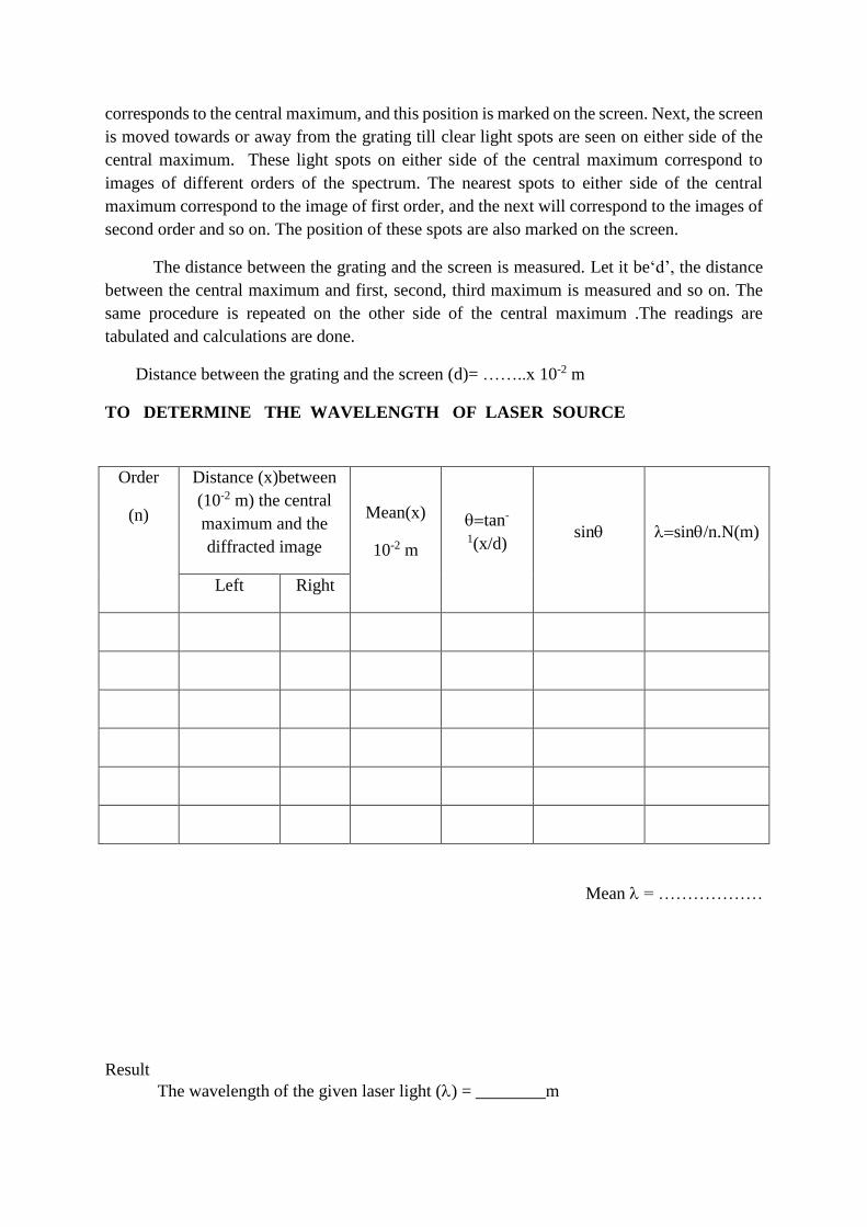
corresponds to the central maximum, and this position is marked on the screen. Next, the screen

is moved towards or away from the grating till clear light spots are seen on either side of the

central maximum. These light spots on either side of the central maximum correspond to

images of different orders of the spectrum. The nearest spots to either side of the central

maximum correspond to the image of first order, and the next will correspond to the images of

second order and so on. The position of these spots are also marked on the screen.

The distance between the grating and the screen is measured. Let it be‘d’, the distance

between the central maximum and first, second, third maximum is measured and so on. The

same procedure is repeated on the other side of the central maximum .The readings are

tabulated and calculations are done.

Distance between the grating and the screen (d)= ……..x 10-2 m

TO DETERMINE THE WAVELENGTH OF LASER SOURCE

Mean = ………………

Result

The wavelength of the given laser light () = ________m

Order

(n)

Distance (x)between

(10-2 m) the central

maximum and the

diffracted image

Mean(x)

10-2 m

tan-

1(x/d) sin sin/n.N(m)

Left Right

Ex. No. Date :

6. QUINCKE’S METHOD - DETERMINATION OF MAGNETIC

SUSCEPTIBILITY OF LIQUID AIM

To determine the magnetic susceptibility of the given liquid using Quincke’s method.

APPARATUS REQUIRED

Quincke’s tube with stand, sample liquid (FeCl3), Electromagnet, Constant current

powersupply, Digital Gaussmeter, Travelling Microscope, etc.

Fig. Quincke’s Tube

FORMULA

2gh

χl = ---------- m2 sec-2 gauss-2

H2

Where g - Acceleration due to gravity = 9.8 m/s2

h - Height through which the liquid column rises due to the magnetic field-m H - The magnetic field at the centre of pole pieces - Gauss

PROCEDURE

The apparatus consists of U -shaped tube known as Quincke’s tube. One of the limb of

the tube is wide and the other one narrow. The experimental liquid or solution is filled in the

tube and the narrow limb is placed between the pole pieces of the electromagnet. The

arrangement is in such away that the meniscus in the narrow limb is exactly at the centre of the

pole pieces and the limb vertical.Focus the microscope on the meniscus and take reading (h1).

Apply the magnetic field (H) to its minimum and note its value from the Gauss meter. Note

whether the meniscus rises up or descends down. It rises up for paramagnetic liquids and

descends down for diamagnetic. Refocus the microscope on liquid meniscus and take reading

(h2). Find the difference of two readings to give h = (h1 ~ h2) in m. The experiment is repeated

for different values of applied magnetic field (H) by adjusting the variable power supply of the

electromagnet. In each case, the rise or fall in the liquid meniscus is noted using the travelling

microscope. All the readings are tabulated. From that χl is calculated using the given formula.

OBSERVATION

TO DETERMINE THE MAGNETIC SUSCEPTIBILITY OF A LIQUID

Least Count = 0.001cm

RESULT

The magnetic susceptibility of the given liquid χl = ----------------- m2 sec-2 gauss-2

Initial Reading Current = 0 Magnetic field = 0

Microscope readings

MSR VSC TR = MSR+(VSCXLC)

X10-2m Div X10-2m

S.No Current

in Amp

Magnetic

field in H

Gauss

Microscope reading h = (h1~h2)

X10-2m

h

H2

m/gauss-2

χl

m2 sec-2

gauss-2

Final reading

MSR

X10-2m

VSC

Div

TR = MSR+

(VSCXLC)

X10-2m