pims industrial problem solving workshop pims … seismic image analysis using ... folio returns...
TRANSCRIPT

Proceedings of the Ninth
PIMS Industrial ProblemSolving Workshop
PIMS IPSW 9
Co-sponsored by:
Informatics Circle of Research Excellence,
Alberta Innovation and Science,
The University of Calgary,
and
Natural Sciences and EngineeringResearch Council of Canada
Editor: C. Sean Bohun, Pennsylvania State University


Proceedings of the Ninth Annual
PIMS
Industrial Problem Solving Workshop
Editor: C. Sean Bohun, Pennsylvania State University
Co-sponsored by:
Informatics Circle of Research Excellence,
Alberta Innovation and Science,
The University of Calgary,
Natural Sciences and Engineering Research Council of Canada
May, 2005

π

i
Foreword by the PIMS Director
The PIMS Industrial Problem Solving Workshops have been held annually since 1997. The 9th IPSWwas held at the University of Calgary from May 15–19, 2005, immediately following the 8th GIMMC(Graduate Industrial Mathematics Modelling Camp) which was held at the University of Lethbridge.We are very grateful to the universities for hosting these events.
Approximately 55 participants worked intensely on five problems posed by industrial companiesfrom across North America. All these problems highlight the need for correct mathematical modelling,and the industrial payback from a good solution. We are grateful to Donald Mackenzie (Universityof Calgary), Gerald K. Cole (Biomechanigg Research Inc.), Pierre Lemire & Rob Pinnegar (CalgaryScientific Inc.), Brad Bondy (Genus Capital Management), and Brian Russell (Hampson Russell Soft-ware) for providing the problems and guiding the participants.
Special thanks go to Sean Bohun from Penn State University who carefully edited these proceed-ings, and Elena Braverman and Gary Margrave from the University of Calgary for the difficult task ofproviding the industrial contacts and organizing the meeting.
Dr. Ivar Ekeland, DirectorPacific Institute for the Mathematical Sciences
π

ii
π

Contents
Foreword by the PIMS Director . . . . . . . . . . . . . . . . . . . . . . . . . . . . . . . . . iPreface . . . . . . . . . . . . . . . . . . . . . . . . . . . . . . . . . . . . . . . . . . . . . . 1
1 Dinosaur Tails 31.1 Introduction . . . . . . . . . . . . . . . . . . . . . . . . . . . . . . . . . . . . . . . . 31.2 Dimensional Analysis . . . . . . . . . . . . . . . . . . . . . . . . . . . . . . . . . . . 51.3 Inextensible Rod Equations . . . . . . . . . . . . . . . . . . . . . . . . . . . . . . . . 7
1.3.1 Boundary Conditions and Initial Conditions . . . . . . . . . . . . . . . . . . . 101.3.2 Small Deflection Approximation . . . . . . . . . . . . . . . . . . . . . . . . . 11
1.4 Discrete Block Model . . . . . . . . . . . . . . . . . . . . . . . . . . . . . . . . . . . 111.5 Conclusion . . . . . . . . . . . . . . . . . . . . . . . . . . . . . . . . . . . . . . . . 131.6 Acknowledgements . . . . . . . . . . . . . . . . . . . . . . . . . . . . . . . . . . . . 14
2 Force-Control for the AFTS 172.1 Introduction . . . . . . . . . . . . . . . . . . . . . . . . . . . . . . . . . . . . . . . . 172.2 Closed-loop Force Control . . . . . . . . . . . . . . . . . . . . . . . . . . . . . . . . 192.3 Stewart Platform Dynamics . . . . . . . . . . . . . . . . . . . . . . . . . . . . . . . . 212.4 Feasibility Study . . . . . . . . . . . . . . . . . . . . . . . . . . . . . . . . . . . . . 222.5 Movement Path Parameterization . . . . . . . . . . . . . . . . . . . . . . . . . . . . . 252.6 Conclusions . . . . . . . . . . . . . . . . . . . . . . . . . . . . . . . . . . . . . . . . 26
3 Seismic Image Analysis Using Local Spectra 313.1 Introduction . . . . . . . . . . . . . . . . . . . . . . . . . . . . . . . . . . . . . . . . 313.2 Problem Description . . . . . . . . . . . . . . . . . . . . . . . . . . . . . . . . . . . 313.3 Spectral Background . . . . . . . . . . . . . . . . . . . . . . . . . . . . . . . . . . . 333.4 Addressing Issue One: Identifying Spectral Peaks . . . . . . . . . . . . . . . . . . . . 343.5 Addressing Issue Two: Edge Detection . . . . . . . . . . . . . . . . . . . . . . . . . . 363.6 Addressing Issue Three: Computing the S-transform . . . . . . . . . . . . . . . . . . 363.7 Additional Issues: Stepping Back to Seismic . . . . . . . . . . . . . . . . . . . . . . . 373.8 Acknowledgments . . . . . . . . . . . . . . . . . . . . . . . . . . . . . . . . . . . . 373.9 Appendix . . . . . . . . . . . . . . . . . . . . . . . . . . . . . . . . . . . . . . . . . 37
4 Evaluation of Equity Ranking Models 454.1 Introduction . . . . . . . . . . . . . . . . . . . . . . . . . . . . . . . . . . . . . . . . 454.2 Problem Description . . . . . . . . . . . . . . . . . . . . . . . . . . . . . . . . . . . 45
iii

iv CONTENTS
4.3 Rising to the Challenge . . . . . . . . . . . . . . . . . . . . . . . . . . . . . . . . . . 464.3.1 Ranking . . . . . . . . . . . . . . . . . . . . . . . . . . . . . . . . . . . . . . 474.3.2 Genetic Optimization . . . . . . . . . . . . . . . . . . . . . . . . . . . . . . . 484.3.3 Neural Network . . . . . . . . . . . . . . . . . . . . . . . . . . . . . . . . . . 484.3.4 Constrained Least Squares Optimization . . . . . . . . . . . . . . . . . . . . . 51
4.4 Results . . . . . . . . . . . . . . . . . . . . . . . . . . . . . . . . . . . . . . . . . . . 514.5 Conclusions and Directions for Further Work . . . . . . . . . . . . . . . . . . . . . . 55
5 Seismic Prediction of Reservoir Parameters 595.1 Introduction . . . . . . . . . . . . . . . . . . . . . . . . . . . . . . . . . . . . . . . . 595.2 Mathematical Statement of the Problem . . . . . . . . . . . . . . . . . . . . . . . . . 605.3 Previous Approaches . . . . . . . . . . . . . . . . . . . . . . . . . . . . . . . . . . . 61
5.3.1 Multilinear Regression . . . . . . . . . . . . . . . . . . . . . . . . . . . . . . 625.3.2 GRNN and RBFN . . . . . . . . . . . . . . . . . . . . . . . . . . . . . . . . 635.3.3 Results . . . . . . . . . . . . . . . . . . . . . . . . . . . . . . . . . . . . . . 645.3.4 Challenges . . . . . . . . . . . . . . . . . . . . . . . . . . . . . . . . . . . . 64
5.4 Generalized Additive Model . . . . . . . . . . . . . . . . . . . . . . . . . . . . . . . 645.4.1 Introduction of Generalized Additive Model . . . . . . . . . . . . . . . . . . . 645.4.2 Advantages of GAM . . . . . . . . . . . . . . . . . . . . . . . . . . . . . . . 665.4.3 Fitting GAM . . . . . . . . . . . . . . . . . . . . . . . . . . . . . . . . . . . 665.4.4 Results . . . . . . . . . . . . . . . . . . . . . . . . . . . . . . . . . . . . . . 67
5.5 The Spline Method . . . . . . . . . . . . . . . . . . . . . . . . . . . . . . . . . . . . 675.5.1 Introduction of the Spline Method . . . . . . . . . . . . . . . . . . . . . . . . 675.5.2 Improvement of the Spline Method . . . . . . . . . . . . . . . . . . . . . . . 695.5.3 Results and Analysis . . . . . . . . . . . . . . . . . . . . . . . . . . . . . . . 69
5.6 Discussion . . . . . . . . . . . . . . . . . . . . . . . . . . . . . . . . . . . . . . . . . 705.7 Acknowledgements . . . . . . . . . . . . . . . . . . . . . . . . . . . . . . . . . . . . 71
A List of Participants 79
π
List of Figures
1.1 Anatomical details of the tail base structure in dinosaurs. . . . . . . . . . . . . . . . . 4
1.2 Diplodocus carnegii is a 24m sauropod with a 14m long tail. . . . . . . . . . . . . . . 4
1.3 Comparison of the tail structures for Compsognathus and Tyrannosaurus. . . . . . . . 5
1.4 Ltail as a function of Lleg for a sample of bipedal and quadrupedal dinosaurs. . . . . . . 6
1.5 Scatter plot of the data assumed to satisfy (1.1) and the corresponding plot of the datawhen a and b are chosen to minimize the variance. . . . . . . . . . . . . . . . . . . . . 7
1.6 An effective dinosaur with the major anatomical structures replaced with blocks of arepresentative size. . . . . . . . . . . . . . . . . . . . . . . . . . . . . . . . . . . . . 8
1.7 To the left a rod segment of length ∆s experiences internal forces of F , G, a bendingmoment M and an external force per unit length of ~P . To the right a portion of therod is bent through an angle φ. If the normal to the cross section remains normal, thedisplacement u = yφ. . . . . . . . . . . . . . . . . . . . . . . . . . . . . . . . . . . . 9
1.8 Each block is characterized by a mass of ρAiLi where Ai and Li are the cross sectionalarea and the length of the ith block. Forces and moments Fi, Gi,Mi act to the left ofthe ith black and the segments are connected to one another by a stiff joint that allowsrotation but no extension. The grey area can be thought of as a uniform distribution ofcollagen springs with a spring constant ki. . . . . . . . . . . . . . . . . . . . . . . . . 12
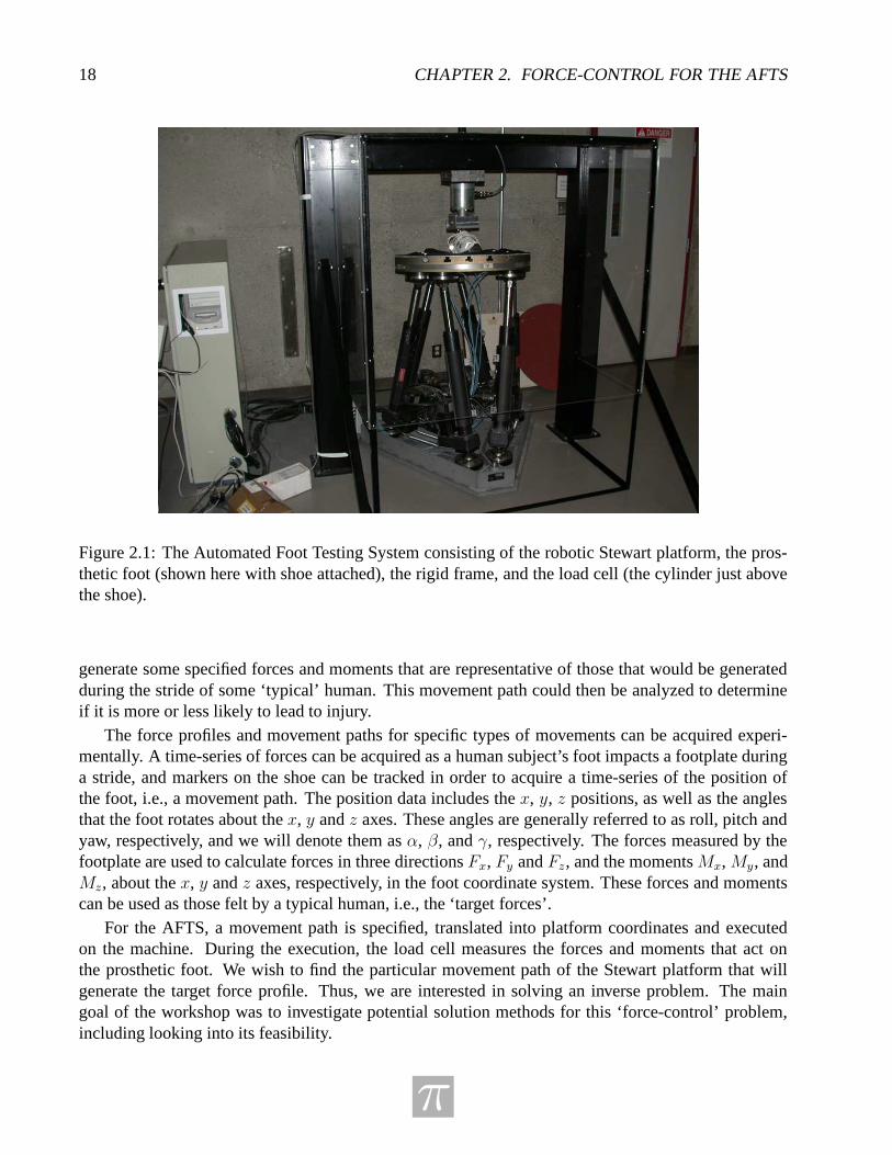
2.1 The Automated Foot Testing System consisting of the robotic Stewart platform, theprosthetic foot (shown here with shoe attached), the rigid frame, and the load cell (thecylinder just above the shoe). . . . . . . . . . . . . . . . . . . . . . . . . . . . . . . . 18
2.2 Three different origins of the platform coordinate system. . . . . . . . . . . . . . . . . 22
2.3 Platform dynamics. (a) A portion of a typical path taken by platform; kinks occur atthe way-points, (b) three different paths corresponding to the three different ‘platformorigins’ depicted in Figure 2.2. . . . . . . . . . . . . . . . . . . . . . . . . . . . . . . 23
2.4 An elastic block of unit length and height. Lower boundary conditions for the dis-placements u(x, y) and v(x, y) are different for the three different cases that are stud-ied (corresponding to different values of the constants a, b, and c), while the side andupper boundary conditions are the same. . . . . . . . . . . . . . . . . . . . . . . . . 24
v

vi LIST OF FIGURES
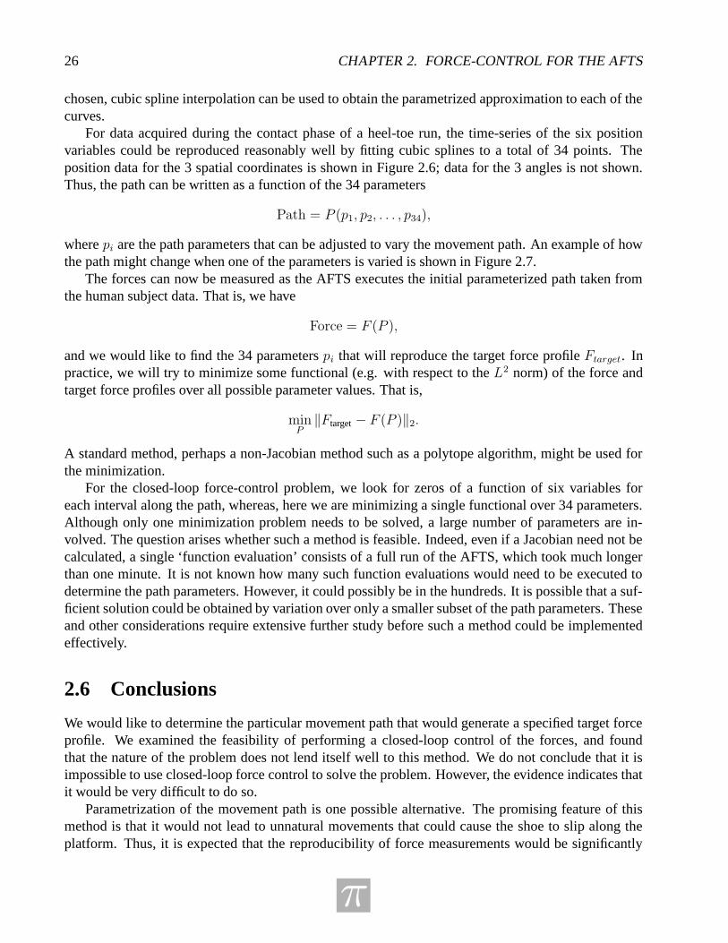
2.5 The two curves in the left panels represent two different sets of boundary conditions,i.e. of the constants a and b representing the amount of compression at the bottomboundary and slope of the bottom boundary, respectively, where the y-axis gives thevalues of the constants and the x-axis represents a parametrization for the changesin the constants. The curves in the right panels show the resulting differences in theforces, i.e., large changes in the boundary conditions only result in small changes inthe forces, where the y-axis gives the values of the forces and the x-axis represents thesame parametrization as in the left panels. . . . . . . . . . . . . . . . . . . . . . . . . 28
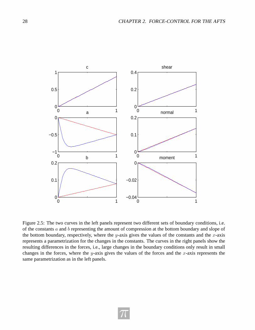
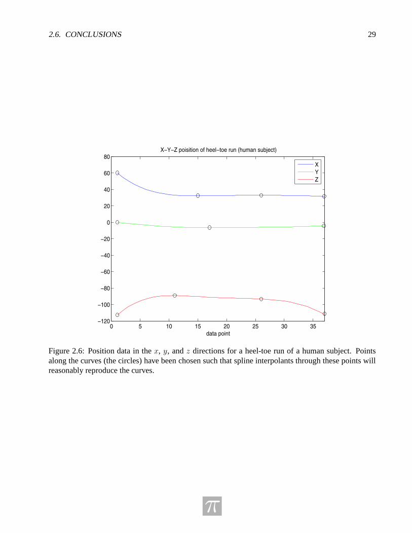
2.6 Position data in the x, y, and z directions for a heel-toe run of a human subject. Pointsalong the curves (the circles) have been chosen such that spline interpolants throughthese points will reasonably reproduce the curves. . . . . . . . . . . . . . . . . . . . . 29
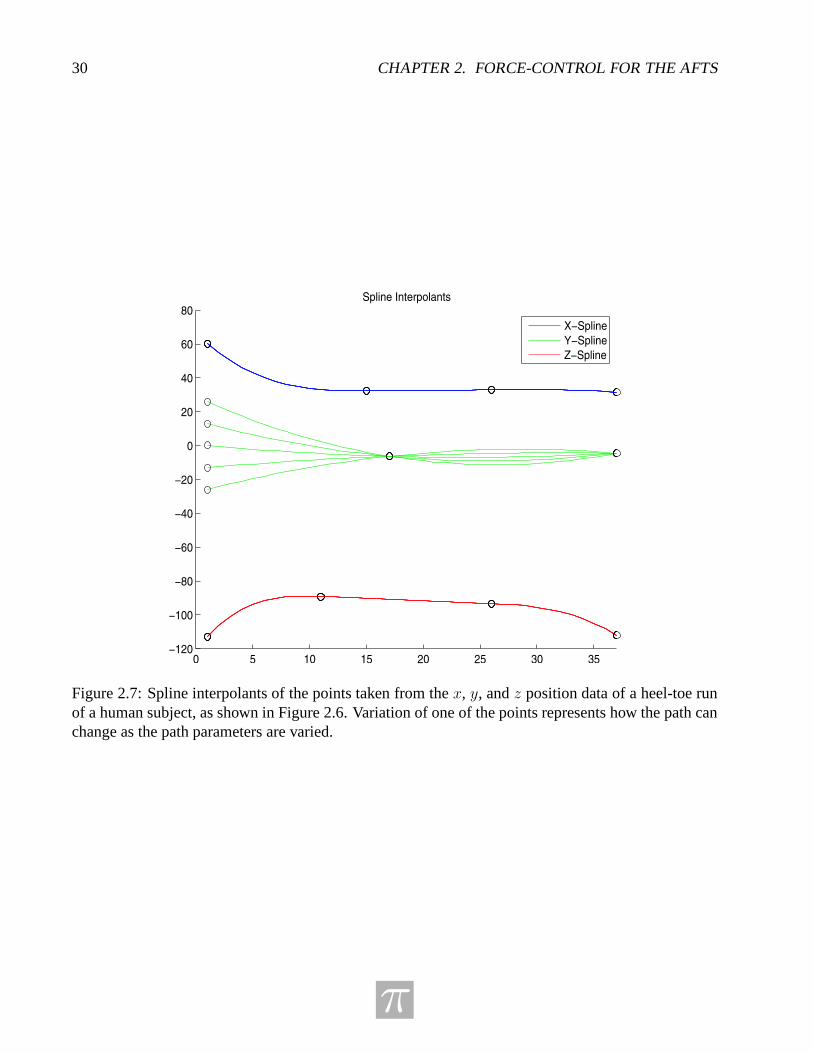
2.7 Spline interpolants of the points taken from the x, y, and z position data of a heel-toe run of a human subject, as shown in Figure 2.6. Variation of one of the pointsrepresents how the path can change as the path parameters are varied. . . . . . . . . . 30
3.1 A sample seismic section. . . . . . . . . . . . . . . . . . . . . . . . . . . . . . . . . . 323.2 A typical local spectrum. . . . . . . . . . . . . . . . . . . . . . . . . . . . . . . . . . 333.3 A sequence of peaks being subtracted from the data. . . . . . . . . . . . . . . . . . . . 35
4.1 Factor weights from the genetic algorithm. . . . . . . . . . . . . . . . . . . . . . . . . 494.2 Slice view of the 34-dimensional objective function near the chosen maximum for the
genetic optimisation. The first graph shows the limits of the weight values, as well asthe value of the objective function at ~w0. In each of the other graphs the vertical linedenotes the value of the corresponding component of ~w0. . . . . . . . . . . . . . . . . 50
4.3 Factor weights from the constrained least squares optimisation. . . . . . . . . . . . . . 524.4 Three-year results from the constrained least-squares model, the genetic optimisation
model, and the neural network. . . . . . . . . . . . . . . . . . . . . . . . . . . . . . . 534.5 Values of Hit Ratio, Excess Information Ratio, Excess Information Ratio (using port-
folio returns relative to the index), Annual Excess Return and Annual Return for theportfolios generated by the three different ranking models. . . . . . . . . . . . . . . . 54
5.1 Elastic waves are sent into the earth and the reflected signals from the subsurface layersare recorded on the surface as a function of time. . . . . . . . . . . . . . . . . . . . . 60
5.2 Here is the inversion of a seismic line from the survey, showing a channel sand ata time of 1075 ms and the intersection of well 08-08. The values are in impedance(velocity·density) and we wish to predict velocity. . . . . . . . . . . . . . . . . . . . . 61
5.3 The well logging procedure directly obtains high resolution values of the desired pa-rameters. . . . . . . . . . . . . . . . . . . . . . . . . . . . . . . . . . . . . . . . . . . 62
5.4 The basic prediction problem, where we want to predict tj from xj . . . . . . . . . . . . 635.5 The true (red) and predicted (blue) values of velocity Y vs. time (Well 11–the best case). 655.6 The true (red) and predicted (blue) values of velocity Y vs. time (Well 5–the worst case). 665.7 The true (red) and predicted (blue) values of velocity Y vs. time (Well 6 –the best case). 685.8 The true (red) and predicted (blue) values of velocity Y vs. time (Well 5–the worst case). 695.9 Scatter plots of the target versus the attributes. Attribute 1 is the impedance, and it is
the only attribute that displays a significant correlation. . . . . . . . . . . . . . . . . . 70
π

LIST OF FIGURES vii
5.10 Improving the Spline Method. . . . . . . . . . . . . . . . . . . . . . . . . . . . . . . 715.11 The true (red) and predicted (blue) values of velocity Y vs. time (Well 6–the best case). 725.12 The true (red) and predicted (blue) values of velocity Y vs. time (Well 9–the worst case). 725.13 The true (red) and predicted (blue) values of the velocity Y vs. time for a typical
example in the study. Notice that the rapidly changing features are very hard to predictcorrectly. . . . . . . . . . . . . . . . . . . . . . . . . . . . . . . . . . . . . . . . . . 73
5.14 The location of the 12 wells in a particular depth plane, with the blue well signifyingthe well to be predicted. . . . . . . . . . . . . . . . . . . . . . . . . . . . . . . . . . . 74
5.15 A spline fit in a given depth plane. . . . . . . . . . . . . . . . . . . . . . . . . . . . . 745.16 The true (red) and the predicted (blue) values for the velocity Y vs. time for the local
depth spline estimator. . . . . . . . . . . . . . . . . . . . . . . . . . . . . . . . . . . 75
π

viii LIST OF FIGURES
π
1
Preface
The University of Calgary was the site of the ninth annual PIMS Industrial Problem Solving Workshop(IPSW). Hosted from May 15 through May 19, 2005, the workshop was co-sponsored by PIMS, Al-berta Innovation and Science, iCORE and the University of Calgary. This workshop saw the bringingtogether of participants from across North America.
Many first time participants of these workshops are surprised by the intensity of the work. Basedon the Oxford Study Group Model, the morning of the first day consists of the initial problem pre-sentations and the beginning of focused discussions amongst the self-selected groups. Input from theacademic experts was found to be especially vital during the initial phases the work, especially in pro-viding guidance to the new participants and graduate students. Work continued throughout the nextfew days culminating in a summary presentation of results at the end of the fifth day. These summarypresentations form the basis of these proceedings. Problems were chosen from a diverse set of topicswhich challenged the participants and utilized many of their individual talents. I would like to takethis opportunity to thank the individual authors for their dedication and prompt response so that theseproceedings were possible. These individuals were (in order of their submission):
• Tony Ware: Adaptive Statistical Evolution Tools for Equity Ranking Models
• Greg Lewis: Force-Control for the Automated Footwear Testing System
• Michael Lamoureux: Seismic Image Analysis Using Local Spectra
• Yaling Yin: Seismic Prediction of Reservoir Parameters
• C. Sean Bohun: Mathematical Model of the Mechanics and Dynamics of Tails in Dinosaurs
To ensure the smooth and efficient operation of the workshop, many individuals are needed behindthe scenes. I would like to thank the organizing committee consisting of Elena Braverman and GaryMargrave both from the University of Calgary. Without their dedication and resourcefulness, this eventwould not have been possible.
Two other essential ingredients for the success of the workshop were the industrial representativesand the industrial experts. While the representatives are certainly an asset and provide a basis for eachof the problems, it is the academic experts that are responsible for each of the groups moving alongproductive lines. For this year the academic experts were:
• C. Sean Bohun, Pennsylvania State University
• Len Bos, University of Calgary
• Elena Braverman, University of Calgary
• Gemai Chen, University of Calgary
• Lou Fishman, MDF International, University of Calgary
• Michael Lamoureux, University of Calgary
• Greg Lewis, University of Ontario Institute of Technology
π

2
• Qiao Sun, University of Calgary
• Tony Ware, University of Calgary
• Rex Westbrook, University of Calgary
A special thanks goes to the industrial contributors and their representatives who include:
• Donald M. Henderson, University of Calgary in collaboration with the Royal Tryell Museum ofPalaeontology
• Gerald K. Cole, University of Calgary in collaboration with Biomechanigg Research Inc.
• Rob Pinnegar, Calgary Scientific Inc.
• Pierre Lemire, Calgary Scientific Inc.
• Brad Bondy, Genus Capital Management
• Brian Russell, Hampson-Russell Software
At the end of this monograph there is a listing of the workshop participants and the various institu-tions where they can be found and I would like to take this opportunity to apologize for any mistakesor omissions therein.
In closing, I would like to thank Heather Jenkins at the PIMS central office for her dedication,efficiency, and patience in dealing with the production of these proceedings.
C. Sean Bohun, EditorDepartment of MathematicsPennsylvania State University
π

Chapter 1
Mathematical Model of the Mechanics andDynamics of the Tails in Dinosaurs
Problem presented by: Donald Mackenzie (University of Calgary)
Mentors: C. Sean Bohun (Pennsylvania State University), Donald Henderson (University of Calgary),Bernard Monthubert (Institut de Mathematiques de Toulouse), Rex Westbrook (University of Calgary)
Student Participants: Robin Clysdale (University of Calgary), Diana David-Rus (Rutgers Univer-sity), Matthew Emmett (University of Calgary), Chad Hogan (University of Calgary), Mark Hughes(University of Calgary), Enkeleida Lushi (Simon Fraser University), Peter Smith (Memorial Universityof Newfoundland), Naveen Vaidya (York University)
Report prepared by: C. Sean Bohun ([email protected])
1.1 Introduction
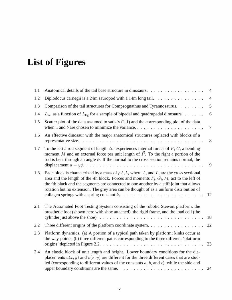
Unlike mammals which have very reduced tails, the tails of dinosaurs represented a substantial fractionof their body lengths and masses. The left and right sides of the tail base in all dinosaurs acted asthe anchor points for large, powerful muscles that attached on the rearward side of the hind limbs(Figure 1.1). These muscles pulled on the legs, causing them to rotate backwards and under the body,with the result that the animals were propelled forward. As well as pulling on the legs, these muscleswould have exerted a reciprocal pull on the tail. During locomotion the left and right hind limbs wouldbe alternately pulled, and be 180◦ out of phase with each other. These alternating tugs would have setup oscillations in the tail. It would seem that some sort of synchrony would have to arise between therate at which the legs were swung back and forth and the natural frequencies of oscillations of the tailto allow efficient, stable walking and running. The extreme sizes of some dinosaurs—up to 30 tonnesin some cases—and the great range of body sizes—from a few hundred grams to many tonnes—givesdinosaurs the potential to be insightful models for the study of locomotory dynamics in terrestrialanimals.
There are two possible avenues to investigate the effects of tails on locomotion:
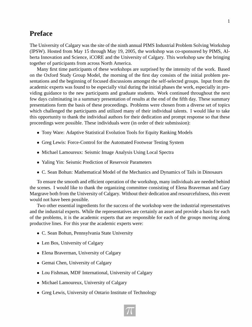
1. Focus on just the ∼ 14m tail of Diplodocus carnegii, a 24m sauropod where the tail representsapproximately 26% of the total body mass detailed in Figure 1.2.
3
4 CHAPTER 1. DINOSAUR TAILS
Figure 1.1: Anatomical details of the tail base structure in dinosaurs.
Figure 1.2: Diplodocus carnegii is a 24m sauropod with a 14m long tail.
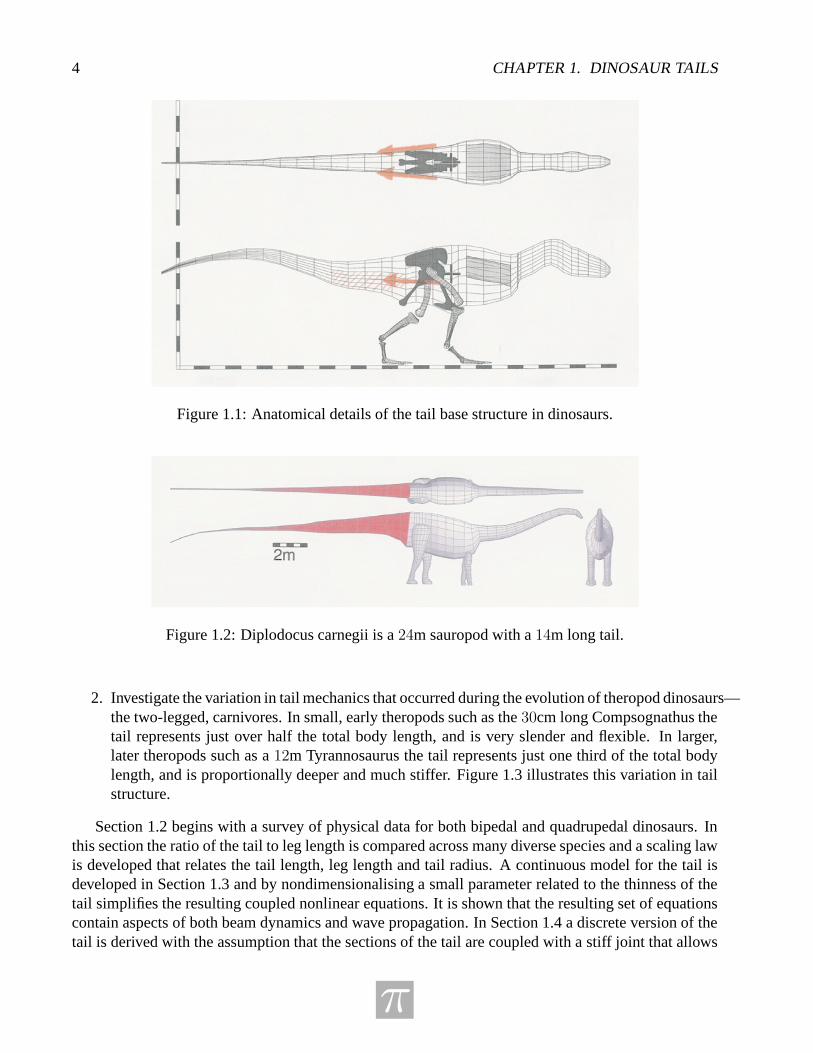
2. Investigate the variation in tail mechanics that occurred during the evolution of theropod dinosaurs—the two-legged, carnivores. In small, early theropods such as the 30cm long Compsognathus thetail represents just over half the total body length, and is very slender and flexible. In larger,later theropods such as a 12m Tyrannosaurus the tail represents just one third of the total bodylength, and is proportionally deeper and much stiffer. Figure 1.3 illustrates this variation in tailstructure.
Section 1.2 begins with a survey of physical data for both bipedal and quadrupedal dinosaurs. Inthis section the ratio of the tail to leg length is compared across many diverse species and a scaling lawis developed that relates the tail length, leg length and tail radius. A continuous model for the tail isdeveloped in Section 1.3 and by nondimensionalising a small parameter related to the thinness of thetail simplifies the resulting coupled nonlinear equations. It is shown that the resulting set of equationscontain aspects of both beam dynamics and wave propagation. In Section 1.4 a discrete version of thetail is derived with the assumption that the sections of the tail are coupled with a stiff joint that allows
π

1.2. DIMENSIONAL ANALYSIS 5
Figure 1.3: Comparison of the tail structures for Compsognathus and Tyrannosaurus.
rotation but does not allow extension. In this model the stiffness of each joint is characterized by aneffective spring constant ki for the ith joint and results in a discrete version of the Euler-Bernoulliexpression for each of the tail segments. The paper finishes with some preliminary conclusions anddirections for future work.
1.2 Dimensional Analysis
As a first model we suppose that the tail acts like a flexible beam with the periodic driving force ofthe rear legs modelled with a pendulum. If the beam has length Ltail and effective radius Rtail then thedeflection of the beam u(x, t) : [0, Ltail] × [0,∞) → R is given by
∂2
∂x2
(
EI(x)∂2u
∂x2
)
= ρA(x)∂2u
∂t2
where E is the Young’s modulus, I is the moment of inertia about the neutral axis, ρ is the density,and A is the cross section of the tail. If we nondimensionise by substituting
x =x
Ltail, u =
u
Ltail, t =
t
Ttail,
I = R4tailI , A = R2
tailA
π
6 CHAPTER 1. DINOSAUR TAILS
we find thatER2
tailT2tail
ρL4tail
∂2
∂x2
(
I∂2u
∂x2
)
= A∂2u
∂t2.
This indicates that the characteristic time to propagate a disturbance the complete length of the tail is
Ttail ∼( ρ
E
)1/2 L2tail
Rtail.
At the same level of approximation assume that the legs of the dinosaur act like a pendulum oflength Lleg so that the characteristic period for the motion of the legs is on the order of
Tleg ∼(
Lleg
g
)1/2
where g is the acceleration due to gravity. As a result, if the tail plays a significant role in the locomo-tion with this model then Tleg ∼ Ttail and
L4tail
LlegR2tail
= const. (1.1)
depending only on the composition of the tail. Notice that this expression predicts that for a fixed leglength, increasing the length of the tail necessarily increases its effective radius in contrast with thearchaeological evidence.
-1 -0.5 0 0.5 1 -0.5
0
0.5
1
1.5
log10(Lleg)
log 1
0(L
tail)
Biped: Ltail = 1.99Lleg1.14
Quadruped: Ltail = 2.73Lleg1.18
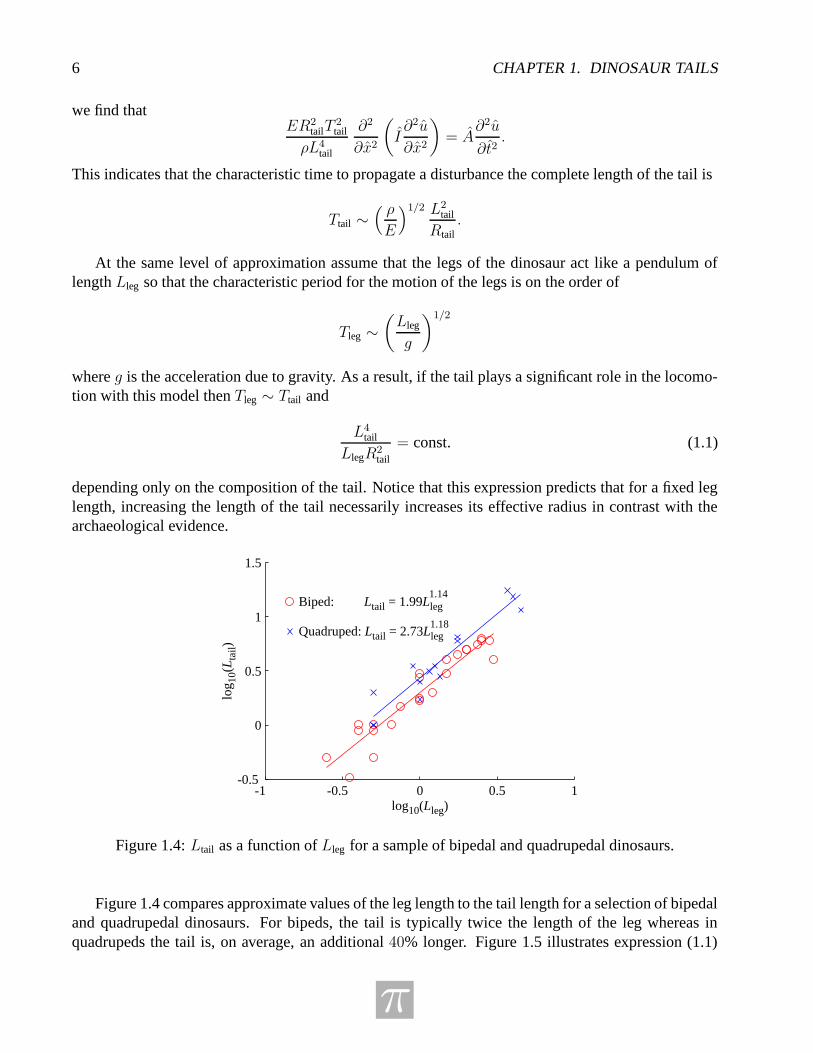
Figure 1.4: Ltail as a function of Lleg for a sample of bipedal and quadrupedal dinosaurs.
Figure 1.4 compares approximate values of the leg length to the tail length for a selection of bipedaland quadrupedal dinosaurs. For bipeds, the tail is typically twice the length of the leg whereas inquadrupeds the tail is, on average, an additional 40% longer. Figure 1.5 illustrates expression (1.1)
π
1.3. INEXTENSIBLE ROD EQUATIONS 7
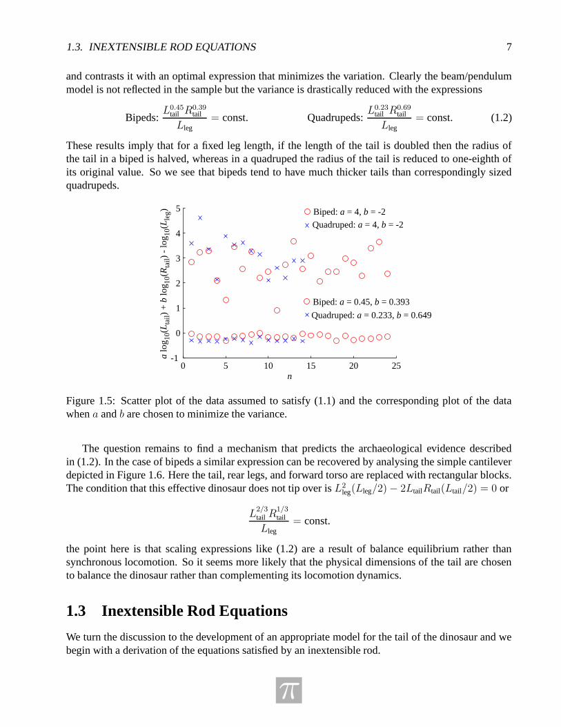
and contrasts it with an optimal expression that minimizes the variation. Clearly the beam/pendulummodel is not reflected in the sample but the variance is drastically reduced with the expressions
Bipeds:L0.45
tail R0.39tail
Lleg= const. Quadrupeds:
L0.23tail R
0.69tail
Lleg= const. (1.2)
These results imply that for a fixed leg length, if the length of the tail is doubled then the radius ofthe tail in a biped is halved, whereas in a quadruped the radius of the tail is reduced to one-eighth ofits original value. So we see that bipeds tend to have much thicker tails than correspondingly sizedquadrupeds.
0 5 10 15 20 25 -1
0
1
2
3
4
5
n
a lo
g 10(
Lta
il) +
b lo
g 10(
Rta
il) -
log 1
0(L
leg) Biped: a = 4, b = -2
Biped: a = 0.45, b = 0.393
Quadruped: a = 4, b = -2
Quadruped: a = 0.233, b = 0.649
Figure 1.5: Scatter plot of the data assumed to satisfy (1.1) and the corresponding plot of the datawhen a and b are chosen to minimize the variance.
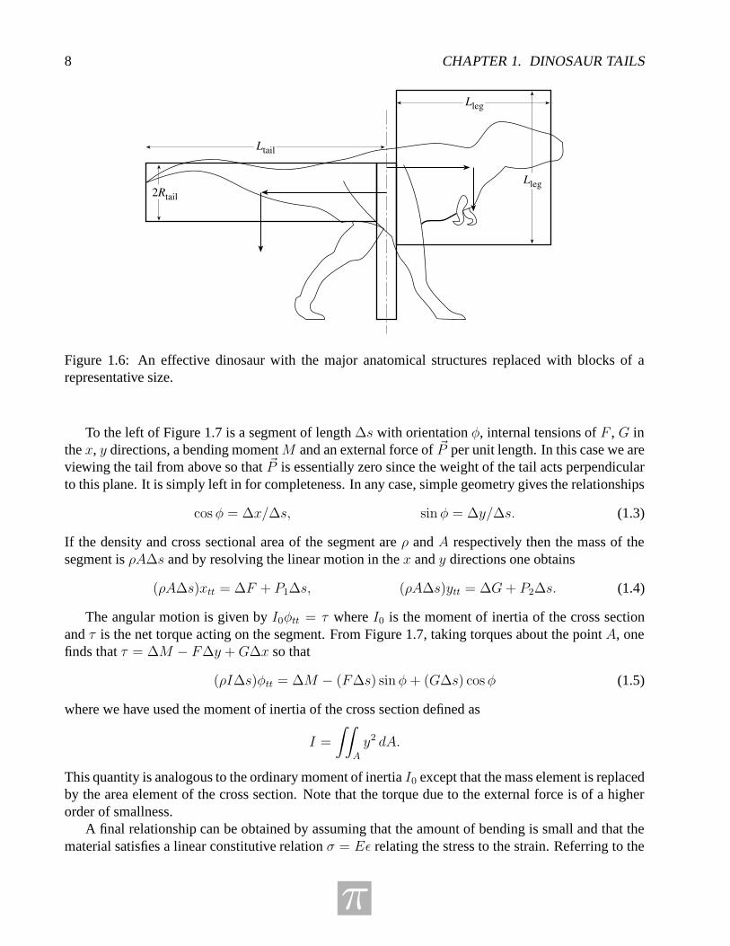
The question remains to find a mechanism that predicts the archaeological evidence describedin (1.2). In the case of bipeds a similar expression can be recovered by analysing the simple cantileverdepicted in Figure 1.6. Here the tail, rear legs, and forward torso are replaced with rectangular blocks.The condition that this effective dinosaur does not tip over is L2
leg(Lleg/2) − 2LtailRtail(Ltail/2) = 0 or
L2/3tail R
1/3tail
Lleg= const.
the point here is that scaling expressions like (1.2) are a result of balance equilibrium rather thansynchronous locomotion. So it seems more likely that the physical dimensions of the tail are chosento balance the dinosaur rather than complementing its locomotion dynamics.
1.3 Inextensible Rod Equations
We turn the discussion to the development of an appropriate model for the tail of the dinosaur and webegin with a derivation of the equations satisfied by an inextensible rod.
π
8 CHAPTER 1. DINOSAUR TAILS
Ltail
Lleg
Lleg2Rtail
Figure 1.6: An effective dinosaur with the major anatomical structures replaced with blocks of arepresentative size.
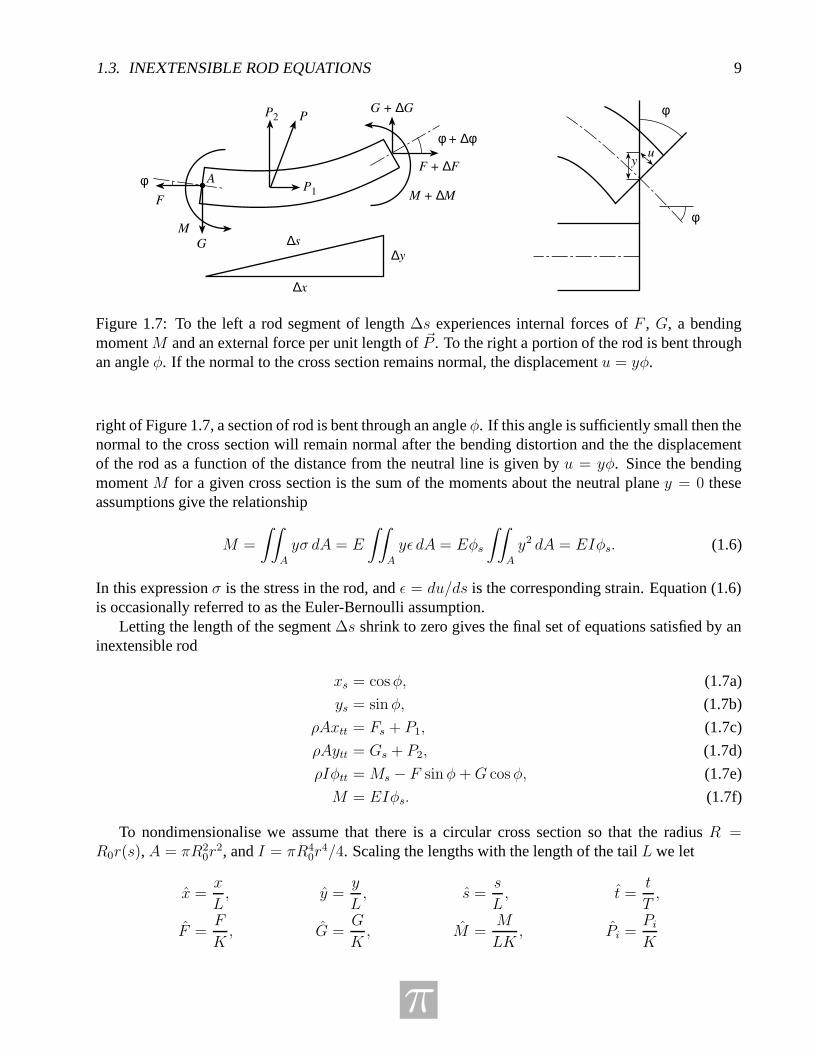
To the left of Figure 1.7 is a segment of length ∆s with orientation φ, internal tensions of F , G inthe x, y directions, a bending momentM and an external force of ~P per unit length. In this case we areviewing the tail from above so that ~P is essentially zero since the weight of the tail acts perpendicularto this plane. It is simply left in for completeness. In any case, simple geometry gives the relationships
cos φ = ∆x/∆s, sinφ = ∆y/∆s. (1.3)
If the density and cross sectional area of the segment are ρ and A respectively then the mass of thesegment is ρA∆s and by resolving the linear motion in the x and y directions one obtains
(ρA∆s)xtt = ∆F + P1∆s, (ρA∆s)ytt = ∆G+ P2∆s. (1.4)
The angular motion is given by I0φtt = τ where I0 is the moment of inertia of the cross sectionand τ is the net torque acting on the segment. From Figure 1.7, taking torques about the point A, onefinds that τ = ∆M − F∆y +G∆x so that
(ρI∆s)φtt = ∆M − (F∆s) sinφ+ (G∆s) cosφ (1.5)
where we have used the moment of inertia of the cross section defined as
I =
∫∫
A
y2 dA.
This quantity is analogous to the ordinary moment of inertia I0 except that the mass element is replacedby the area element of the cross section. Note that the torque due to the external force is of a higherorder of smallness.
A final relationship can be obtained by assuming that the amount of bending is small and that thematerial satisfies a linear constitutive relation σ = Eε relating the stress to the strain. Referring to the
π
1.3. INEXTENSIBLE ROD EQUATIONS 9
∆x
∆y∆s
φ
φ
uy
M
M + ∆MF
G
G + ∆G
F + ∆Fφ
φ + ∆φ
A
PP2
P1
Figure 1.7: To the left a rod segment of length ∆s experiences internal forces of F , G, a bendingmoment M and an external force per unit length of ~P . To the right a portion of the rod is bent throughan angle φ. If the normal to the cross section remains normal, the displacement u = yφ.
right of Figure 1.7, a section of rod is bent through an angle φ. If this angle is sufficiently small then thenormal to the cross section will remain normal after the bending distortion and the the displacementof the rod as a function of the distance from the neutral line is given by u = yφ. Since the bendingmoment M for a given cross section is the sum of the moments about the neutral plane y = 0 theseassumptions give the relationship
M =
∫∫
A
yσ dA = E
∫∫
A
yε dA = Eφs
∫∫
A
y2 dA = EIφs. (1.6)
In this expression σ is the stress in the rod, and ε = du/ds is the corresponding strain. Equation (1.6)is occasionally referred to as the Euler-Bernoulli assumption.
Letting the length of the segment ∆s shrink to zero gives the final set of equations satisfied by aninextensible rod
xs = cosφ, (1.7a)
ys = sinφ, (1.7b)
ρAxtt = Fs + P1, (1.7c)
ρAytt = Gs + P2, (1.7d)
ρIφtt = Ms − F sinφ+G cosφ, (1.7e)
M = EIφs. (1.7f)
To nondimensionalise we assume that there is a circular cross section so that the radius R =R0r(s), A = πR2
0r2, and I = πR4
0r4/4. Scaling the lengths with the length of the tail L we let
x =x
L, y =
y
L, s =
s
L, t =
t
T,
F =F
K, G =
G
K, M =
M
LK, Pi =
Pi
K
π
10 CHAPTER 1. DINOSAUR TAILS
and identify three nondimensional quantities C1 = πρR20L
2/KT 2, C2 = πρR40/4KT
2 and C3 =4KL2/πER4
0. The characteristic magnitudes of the force and time should reflect the physical proper-ties of the tail. Consider a rod of length L which is clamped horizontally at one end, free at the other,and bends under its own weight. If the rod has mass m and g is the gravitational constant then theshape satisfies
ζ(iv) =mg/L
EI, ζ(0) = ζ ′(0) = ζ ′′(L) = ζ ′′′(L) = 0,
with solution
ζ(s) =mg/L
24EIs2(s2 − 4Ls + 6L2)
and a maximum displacement at s = L that satisfies
ζ(L)
L=
1
8
mg
L2/EI.
In this case the characteristic force for a rod that bends under its own weight is K = EI/L2 andchoosing this value for K sets C3 = 1. This leaves two natural choices for T . Either T = L
√
ρ/E orT = 2L2
√
ρ/E/R0 in which C2 = 1 or C1 = 1 respectively. We choose the latter consequently
T 2 =4ρπL4
ER20
=ρπR2
0L4
EI,
C1 = 1, and C2 = (R0/2L)2 is a small parameter for a long thin tail and is denoted as ε.Dropping hats the nondimensional equations are
xs = cosφ, (1.8a)
ys = sinφ, (1.8b)
r2(s)xtt = Fs + P1, (1.8c)
r2(s)ytt = Gs + P2, (1.8d)
εr4(s)φtt = Ms − F sinφ+G cosφ, (1.8e)
M = r4(s)φs (1.8f)
with 0 ≤ s ≤ 1, and r(s) = R(s)/R0 a nondimensional radius of the rod. Since ε is small, equa-tion (1.8e) implies that if initially τ(s) = Ms − F sin φ + G cosφ 6= 0 then φ will change rapidlywith time until τ = 0. Conversely, equations (1.8c) and (1.8d) indicate that x and y will not appre-ciably change during this equalization process. On the time scale of T , the ε term can be omitted andexpression (1.8e) can be replaced with
τ(s) = Ms − F sin φ+G cosφ = 0.
1.3.1 Boundary Conditions and Initial Conditions
Since the tip of the tail (s = 1) is free, the internal forces and bending moments vanish so thatF = G = M = 0. At the base (s = 0) it is not clear if one should consider a clamped, hinged, or
π
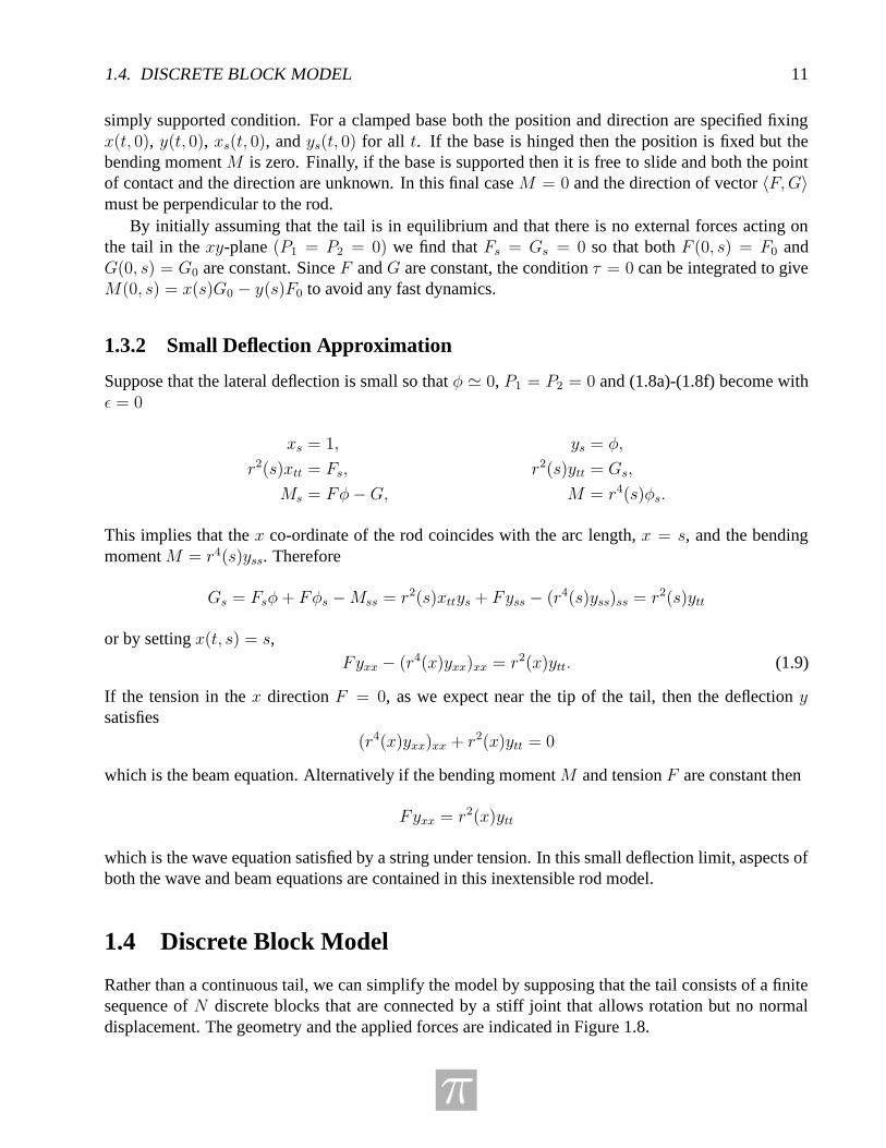
1.4. DISCRETE BLOCK MODEL 11
simply supported condition. For a clamped base both the position and direction are specified fixingx(t, 0), y(t, 0), xs(t, 0), and ys(t, 0) for all t. If the base is hinged then the position is fixed but thebending moment M is zero. Finally, if the base is supported then it is free to slide and both the pointof contact and the direction are unknown. In this final case M = 0 and the direction of vector 〈F,G〉must be perpendicular to the rod.
By initially assuming that the tail is in equilibrium and that there is no external forces acting onthe tail in the xy-plane (P1 = P2 = 0) we find that Fs = Gs = 0 so that both F (0, s) = F0 andG(0, s) = G0 are constant. Since F and G are constant, the condition τ = 0 can be integrated to giveM(0, s) = x(s)G0 − y(s)F0 to avoid any fast dynamics.
1.3.2 Small Deflection Approximation
Suppose that the lateral deflection is small so that φ ' 0, P1 = P2 = 0 and (1.8a)-(1.8f) become withε = 0
xs = 1, ys = φ,
r2(s)xtt = Fs, r2(s)ytt = Gs,
Ms = Fφ−G, M = r4(s)φs.
This implies that the x co-ordinate of the rod coincides with the arc length, x = s, and the bendingmoment M = r4(s)yss. Therefore
Gs = Fsφ+ Fφs −Mss = r2(s)xttys + Fyss − (r4(s)yss)ss = r2(s)ytt
or by setting x(t, s) = s,Fyxx − (r4(x)yxx)xx = r2(x)ytt. (1.9)
If the tension in the x direction F = 0, as we expect near the tip of the tail, then the deflection ysatisfies
(r4(x)yxx)xx + r2(x)ytt = 0
which is the beam equation. Alternatively if the bending moment M and tension F are constant then
Fyxx = r2(x)ytt
which is the wave equation satisfied by a string under tension. In this small deflection limit, aspects ofboth the wave and beam equations are contained in this inextensible rod model.
1.4 Discrete Block Model
Rather than a continuous tail, we can simplify the model by supposing that the tail consists of a finitesequence of N discrete blocks that are connected by a stiff joint that allows rotation but no normaldisplacement. The geometry and the applied forces are indicated in Figure 1.8.
π

12 CHAPTER 1. DINOSAUR TAILS
xi,yi
xi+1,yi+1∆φ
φi
φi+1
Mi+1Fi
Gi+1
Fi+1Gi
Mi
Li
Figure 1.8: Each block is characterized by a mass of ρAiLi where Ai and Li are the cross sectionalarea and the length of the ith block. Forces and moments Fi, Gi,Mi act to the left of the ith black andthe segments are connected to one another by a stiff joint that allows rotation but no extension. Thegrey area can be thought of as a uniform distribution of collagen springs with a spring constant ki.
The co-ordinates of the centre of mass of block i+ 1 is given by
xi+1 = xi +Li
2cosφi +
Li+1
2cosφi+1, i = 1, 2, . . . , N − 1
yi+1 = yi +Li
2sin φi +
Li+1
2sinφi+1, i = 1, 2, . . . , N − 1
and the origin is taken so that x1 = y1 = 0. In a similar fashion the net force and bending momentacting on block i give for i = 1, 2, . . . , N − 1
ρAiLixi = Fi+1 − Fi,
ρAiLiyi = Gi+1 −Gi,
ρIiLiφi = Mi+1 −Mi −Li
2(Fi+1 + Fi) sinφi +
Li+1
2(Gi+1 +Gi) cosφi,
where the dots denote differentiation with time. For i = N + 1, Li+1 = 0 and we choose FN+1 =GN+1 = MN+1 = 0 since the last block has a free end. These are simply a discretised version ofthe original extension free equations (1.7a)-(1.7f). What remains is a discrete version of the Euler-Bernoulli expression relating the bending moment to the curvature of the tail.
Suppose that there is a uniform distribution of collagen springs in the gap between blocks i andi+1. Let ki denote the spring constant measured so that a uniform displacement of length li, the springsequilibrium length, generates a restoring force of −ki. In this case the units of ki is force/area ratherthan the standard force/length. If we instead suppose there is an angular displacement of φi+1 − φi =
π
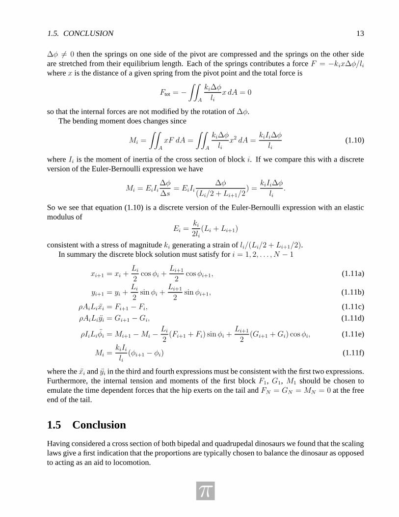
1.5. CONCLUSION 13
∆φ 6= 0 then the springs on one side of the pivot are compressed and the springs on the other sideare stretched from their equilibrium length. Each of the springs contributes a force F = −kix∆φ/liwhere x is the distance of a given spring from the pivot point and the total force is
Ftot = −∫∫
A
ki∆φ
lix dA = 0
so that the internal forces are not modified by the rotation of ∆φ.The bending moment does changes since
Mi =
∫∫
A
xF dA =
∫∫
A
ki∆φ
lix2 dA =
kiIi∆φ
li(1.10)
where Ii is the moment of inertia of the cross section of block i. If we compare this with a discreteversion of the Euler-Bernoulli expression we have
Mi = EiIi∆φ
∆s= EiIi
∆φ
(Li/2 + Li+1/2) =
kiIi∆φ
li.
So we see that equation (1.10) is a discrete version of the Euler-Bernoulli expression with an elasticmodulus of
Ei =ki
2li(Li + Li+1)
consistent with a stress of magnitude ki generating a strain of li/(Li/2 + Li+1/2).In summary the discrete block solution must satisfy for i = 1, 2, . . . , N − 1
xi+1 = xi +Li
2cos φi +
Li+1
2cosφi+1, (1.11a)
yi+1 = yi +Li
2sin φi +
Li+1
2sin φi+1, (1.11b)
ρAiLixi = Fi+1 − Fi, (1.11c)
ρAiLiyi = Gi+1 −Gi, (1.11d)
ρIiLiφi = Mi+1 −Mi −Li
2(Fi+1 + Fi) sinφi +
Li+1
2(Gi+1 +Gi) cosφi, (1.11e)
Mi =kiIili
(φi+1 − φi) (1.11f)
where the xi and yi in the third and fourth expressions must be consistent with the first two expressions.Furthermore, the internal tension and moments of the first block F1, G1, M1 should be chosen toemulate the time dependent forces that the hip exerts on the tail and FN = GN = MN = 0 at the freeend of the tail.
1.5 Conclusion
Having considered a cross section of both bipedal and quadrupedal dinosaurs we found that the scalinglaws give a first indication that the proportions are typically chosen to balance the dinosaur as opposedto acting as an aid to locomotion.
π
14 CHAPTER 1. DINOSAUR TAILS
Two models for the motion of the tail were explored. The first of these was a continuous modeland for small deflections it was shown to include aspects of the dynamics of a thin beam as well asthe dynamics of wave motion. This is very encouraging since both of these behaviours are seen in thetails of modern day animals. Unfortunately the resulting equations are a set of strongly coupled partialdifferential equations and more time is required to fully develop a solution consistent with the massdistribution of a given dinosaur.
To simplify the situation a discrete version of the continuous model was developed where the tailis broken into N blocks joined together with a stiff connection that allows rotation but no extension.Once again the result is a set of strongly coupled equations, but there is improvement. First, we areleft with ordinary differential equations and second, the Euler-Bernoulli equation in the continuousmodel is recovered in the discrete model as a result of the behaviour of the springs in each joint. Insome sense this result is not really unexpected since the discrete model is simply the continuous modelwritten as a numerical implementation of the method of lines.
The next step is to simulate the motion of a tail predicted with the discrete block model for aliving animal to estimate the model predictability. Choosing many segments for the tail of varyingstiffness (Ebone ' 20GPa, Ecollagen ' 1GPa) should produced reasonable dynamics. Once this hasbeen accomplished, one can assess the degree to which a tail would have aided in the locomotion ofpedal and quadrupedal dinosaurs.
1.6 Acknowledgements
The authors would like to acknowledge the Pacific Institute for the Mathematical Sciences (PIMS) fortheir sponsorship of the IPSW. We would also like to take this opportunity to thank the University ofCalgary hospitality in hosting this event and special thank-you is reserved for Elena Braverman andMarian Miles. Their hard work and dedication ensured the success of the workshop.
π

Bibliography
[1] Berger, S.A., Goldsmith, E.W. & Lewis, E.R. (2000). Introduction to Bioengineering. OxfordUniversity Press.
[2] Chouaieb, N. & Maddocks, J.H. (2004). Kirchhoff’s problem of helical equilibria of uniform rods.Journal of Elasticity. 77, pp. 221-247.
[3] Coleman, B.D., Tobias, I. & Swigon, D. (1995). Theory of the influence of end conditions onself-contact in DNA loops. Journal of Chemical Physics. 103(20), pp. 9101-9109.
[4] Dill, E.H. (1992). Kirchhoff’s theory of rods. Archive for History of Exact Sciences. 44(1), pp.1-23.
[5] Goriely, A. & Tabor, M. (2000). The nonlinear dynamics of filaments. Nonlinear Dynamics. 21,pp. 101-133.
[6] Landau, L.D. & Lifshitz, E.M. (1970). Theory of Elasticity, 2nd ed. Pergamon Press: New York.
[7] Nizette, M. & Goriely, A. (1999). Towards a classification of Euler-Kirchhoff filaments. Journalof Mathematical Physics. 40(6), pp. 2830-2866.
[8] Swigon, D., Coleman, B.D. & Tobias, I. (1998). The elastic rod model for DNA and its applicationto the tertiary structure of DNA minicircles and mononucleosomes. Biophysical Journal. 74, pp.2515-2530.
[9] Tam, D., Radovitzky, R. & Samtaney, R. (2005). An algorithm for modelling the interaction of aflexible rod with a two-dimensional high-speed flow. International Journal for Numerical Methodsin Engineering. 64(8), pp. 1057-1077.
[10] Tobias, I., Swigon, D. & Coleman, B.D. (2000). Elastic stability of DNA configurations. I. Gen-eral theory. Physical Review E. 61(1), pp. 747-758.
[11] Woodall, S.R. (1966). The large amplitude oscillations of a thin elastic beam. International Jour-nal of Non-linear Mechanics. 1, pp. 217-238.
[12] Animated dinosaurs:http://palaeo.gly.bris.ac.uk/dinosaur/animation.html
15

16 BIBLIOGRAPHY
[13] Anatomical data:http://internt.nhm.ac.uk/jdsml/nature-online/dino-directory/datafiles.dsml
[14] Dinosaur support information:http://www.ucmp.berkeley.edu/diapsids/saurischia/saurischia.html
http://www.ucmp.berkeley.edu/diapsids/ornithischia/ornithischia.html
http://www.enchantedlearning.com/subjects/dinosaurs/index.html
π
Chapter 2
Force-Control for the Automated FootwearTesting System
Problem presented by: Dr. Gerald K. Cole (Biomechanigg Research Inc.)
Mentors: Greg Lewis (University of Ontario IT), Rex Westbrook (University of Calgary)
Student Participants: Ojenie Artoun (Concordia University), Kent Griffin (Washington State Uni-versity), Jisun Lim (University of Colorado), Xiao Ping Liu (University of Regina), James Odegaard(University of Western Ontario), Sarah Williams (University of California, Davis)
Report prepared by: Greg Lewis ([email protected])
2.1 Introduction
The Automated Footwear Testing System (AFTS) is a robotic system designed to replicated the move-ment and loading of a shoe as it contacts the ground during common human movements. By doing so,the AFTS can serve as a system for the functional testing of different footwear designs in a mannerthat is difficult to achieve by standard testing systems. The AFTS consists of four main components:a robotic Stewart platform, a rigid fixed frame, a load cell and a prosthetic foot. Motion of the footrelative to the ground is created by rigidly fixing the foot to the frame and moving the platform rel-ative to the foot. See Figure 2.1. The Stewart platform has six degrees of kinematic freedom andcan reproduce the required complex three-dimensional motion path within the limitations of its rangeof motion. While the platform is in contact with the footwear, the six-axis load cell measures thethree-dimensional forces and moments acting on the prosthetic foot.
It has been shown that when a human subject performs the same movement with two differentpairs of shoes, she will adjust her stride so that she feels similar forces on her legs, regardless of thefootwear. That is, when testing footwear, it can be assumed that the force profiles will be the same forthe different shoes, while the movement path will differ from shoe to shoe. Thus, a good shoe is a onethat does not lead to an unstable or unnatural movement path, e.g., one that might lead to an overturnedankle, or one that might lead to the need for an overcompensation that could result in an ‘over-use’injury. In order for the AFTS to be most effective at testing a wide variety of design features, it wouldbe necessary to develop a means of determining, for any given shoe, a movement path that would
17
18 CHAPTER 2. FORCE-CONTROL FOR THE AFTS
Figure 2.1: The Automated Foot Testing System consisting of the robotic Stewart platform, the pros-thetic foot (shown here with shoe attached), the rigid frame, and the load cell (the cylinder just abovethe shoe).
generate some specified forces and moments that are representative of those that would be generatedduring the stride of some ‘typical’ human. This movement path could then be analyzed to determineif it is more or less likely to lead to injury.
The force profiles and movement paths for specific types of movements can be acquired experi-mentally. A time-series of forces can be acquired as a human subject’s foot impacts a footplate duringa stride, and markers on the shoe can be tracked in order to acquire a time-series of the position ofthe foot, i.e., a movement path. The position data includes the x, y, z positions, as well as the anglesthat the foot rotates about the x, y and z axes. These angles are generally referred to as roll, pitch andyaw, respectively, and we will denote them as α, β, and γ, respectively. The forces measured by thefootplate are used to calculate forces in three directions Fx, Fy and Fz, and the moments Mx, My, andMz, about the x, y and z axes, respectively, in the foot coordinate system. These forces and momentscan be used as those felt by a typical human, i.e., the ‘target forces’.
For the AFTS, a movement path is specified, translated into platform coordinates and executedon the machine. During the execution, the load cell measures the forces and moments that act onthe prosthetic foot. We wish to find the particular movement path of the Stewart platform that willgenerate the target force profile. Thus, we are interested in solving an inverse problem. The maingoal of the workshop was to investigate potential solution methods for this ‘force-control’ problem,including looking into its feasibility.
π
2.2. CLOSED-LOOP FORCE CONTROL 19
When the same shoe used by the human subject is mounted on the prosthetic foot of the AFTS,and the experimentally measured movement path is replicated on the Stewart platform, the forces andmoments measured to be acting on the prosthetic foot do not match the experimental data. The forcesacting normal to the ground/platform are similar in magnitude for both cases. However, the forcesacting parallel to the ground/platform are not similar. Thus, before using the AFTS to test differentfootwear, it is necessary to determine the platform movement path that leads to the target force profilesfor the ‘control’ shoe, i.e., the shoe used during the acquisition of the target force profile. This may alsobe viewed as a force-control problem. It may be reasonable to use such an approach if the discrepanciesbetween the movement paths for the human subject and platform are relatively small. However, if theyare sufficiently large, it would lead to difficulty in the interpretation of any testing results. That is, thecauses of these discrepancies may reveal information regarding the feasibility of using force-controlas a means of testing footwear. Thus, we seek possible origins of the discrepancies.
We first investigate the possibility of performing a closed-loop control of the forces. That is,we investigate the possibility of adjusting the position of the platform at discrete points along themovement path until the forces measured by the load cell of the AFTS match the target forces at thatpoint. The results, discussed in Section 2.2, indicate that there are some fundamental issues that mustbe considered before the AFTS can reliably be used as a testing system. We study two such issues.The first study looks at the effects due to the choice of the origin of the platform coordinate system.See Section 2.3. This choice might effect how the Stewart platform executes the specified motion,and thus might effect the measured forces. In the second study, presented in Section 2.4, the system ismodelled as a simple elastic body in order to gain some information regarding the feasibility of solvingthe inverse problem. The results suggest that it may be more appropriate to take a global rather thanlocal approach to controlling the forces. In Section 2.5, we discuss the possibility of parameterizingthe movement path using cubic splines, and then minimizing, with respect to the parameters of thecurves, a functional that is small when the measured forces are near the target forces. Conclusionsfollow.
2.2 Closed-loop Force Control
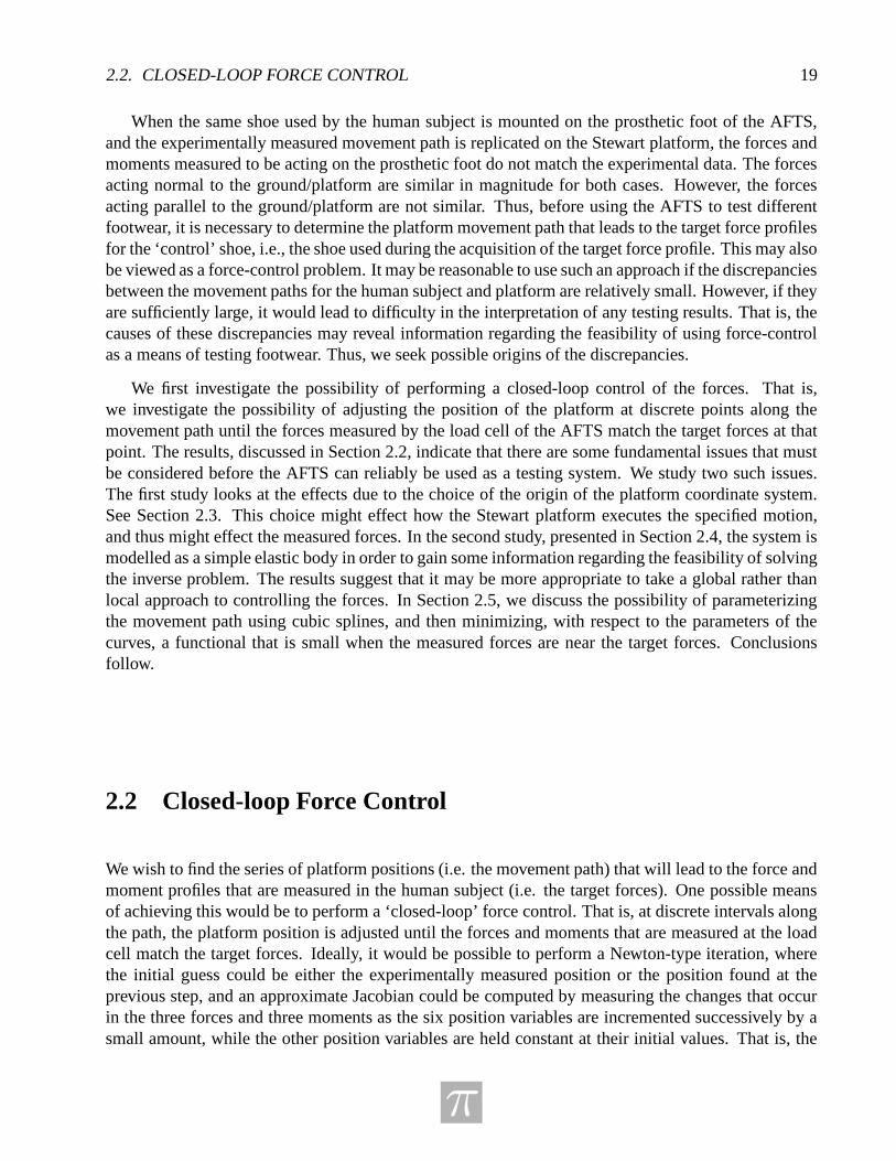
We wish to find the series of platform positions (i.e. the movement path) that will lead to the force andmoment profiles that are measured in the human subject (i.e. the target forces). One possible meansof achieving this would be to perform a ‘closed-loop’ force control. That is, at discrete intervals alongthe path, the platform position is adjusted until the forces and moments that are measured at the loadcell match the target forces. Ideally, it would be possible to perform a Newton-type iteration, wherethe initial guess could be either the experimentally measured position or the position found at theprevious step, and an approximate Jacobian could be computed by measuring the changes that occurin the three forces and three moments as the six position variables are incremented successively by asmall amount, while the other position variables are held constant at their initial values. That is, the
π
20 CHAPTER 2. FORCE-CONTROL FOR THE AFTS
approximate Jacobian could be given by
J =
∆Fx
∆x∆Fx
∆y∆Fx
∆z∆Fx
∆α∆Fx
∆β∆Fx
∆γ
∆Fy
∆x∆Fy
∆y∆Fy
∆z∆Fy
∆α∆Fy
∆β∆Fy
∆γ
∆Fz
∆x∆Fz
∆y∆Fz
∆z∆Fz
∆α∆Fz
∆β∆Fz
∆γ
∆Mx
∆x∆Mx
∆y∆Mx
∆z∆Mx
∆α∆Mx
∆β∆Mx
∆γ
∆My
∆x
∆My
∆y
∆My
∆z
∆My
∆α
∆My
∆β
∆My
∆γ
∆Mz
∆x∆Mz
∆y∆Mz
∆z∆Mz
∆α∆Mz
∆β∆Mz
∆γ
. (2.1)
In practice, this could be computed by incrementing a single position variable, measuring the forces,incrementing that position variable back to its original value, and repeating this for each of the positionvariables. Once the approximate Jacobian is computed, it could be used to choose the next iterate. Theplatform would then be moved into the corresponding position, and the forces would be measured. Ifthe forces are still not sufficiently close to the targets, another iteration could be performed, perhapsvia a quasi-Newton iteration, or perhaps a new Jacobian could be computed. This procedure wouldcontinue until the desired forces are obtained to within a given tolerance. We could then proceed to thenext point along the movement path, and find the platform position corresponding to the target forcesthat are required at this new point.
For this method to be feasible, the computed Jacobians must be non-singular. In order to test this,we computed the approximate Jacobian on the AFTS at two points along the movement path. Themost striking result was that when certain position variables were incremented and returned to theirstarting values, the measured forces did not return to their original values. Even when the positionvariables were incremented by as little as 0.1mm and returned to their original values, the forces andmoments could be as much as 5% different from their starting values.
Upon inspection of the AFTS in use, it was found that certain movements caused the shoe toslip along the platform. Such irreversible behaviour will greatly hinder any force-control procedure.Indeed, the discrepancies between the forces measured for the human subject and those measured forthe platform for the same movement path could be caused to a large extent by the slipping. This isconsistent with the observation that the forces normal to the ground/platform are sufficiently similar,while the tangent forces are not.
It is not surprising that when the approximate Jacobian was formed, we found that it was singular.It was seen, however, that only certain directions were irreversible, and it was speculated that this wascaused by slipping when increments were made in these directions. In order for force-control to bepossible, steps must be taken to reduce the slipping as much as possible. The platform being usedfor the data acquisition was quite worn, which likely exacerbated the problem. Thus, it is possiblethat the installation of a new platform surface designed to limit slipping would greatly improve theprospects. Either way, a method that minimizes slipping, in particular in the specific directions, willgreatly increase the chances of success.
π
2.3. STEWART PLATFORM DYNAMICS 21
2.3 Stewart Platform Dynamics
It is expected that even when steps are taken to reduce slipping, a path-dependence of the forcesmeasured at the load cell will likely linger. Thus, it is not only important to improve reversibility, butalso to maximize reproducibility.
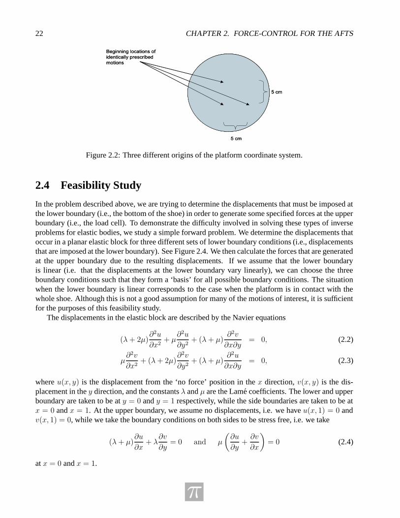
A run of the AFTS begins by raising the platform until it comes in contact with the shoe. Theorigin of the platform coordinate system is chosen as this initial point of contact. Currently, care is nottaken to ensure that this point of contact is the same for each run. However, due to the method thatis used to transform the experimentally measured movement path into platform positions, the choiceof the origin of the platform coordinate system will affect the resulting platform movement path (seebelow). We therefore investigate the magnitude of this effect so that we may determine whether this isa potential cause of error, and whether care must be taken to choose the origin to be the same for eachrun of the AFTS.
Thus, we need to look into the dynamics of the Stewart platform. The platform has six degrees offreedom determined by the length of the actuators (legs), where each set of leg lengths corresponds toa unique position and orientation of the platform.
The actual platform path is not directly specified by the user. The user supplies a series of ‘way-points’, which are a series of positions that the platform must pass through, but the user does not havecontrol over the path that is taken to go from one way-point to the next. The path between each pair ofway-points is determined by an algorithm that requires all actuators to start and stop at the same time.Thus, these intermediate paths may be quite different depending on where the shoe initially contactsthe platform (i.e., the choice of origin for the platform coordinate system). Because we were not ableto test this on the AFTS itself, we performed a theoretical investigation of the path differences thatmight occur for three different origin locations, as shown in Figure 2.2. A central location was chosen,then the two other locations were chosen 5cm away from this central location along the x and y axes,respectively. We computed the platform paths by first computing the leg lengths corresponding to aseries of way-points using the software package designed for this purpose. By assuming that duringthe transition between the way-points all the actuators would start and stop at the same moment, wedetermined a series of leg lengths that would occur between each of the way-points. We then usednumerical methods to invert the nonlinear relation between the leg lengths and platform position, andobtained the intermediate platform positions that corresponded to the intermediate leg lengths.
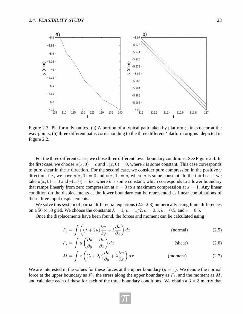
A sample of results is plotted in Figure 2.3. An interesting observation is that the movement pathhas kinks at the way-points. It can also be seen that indeed the paths are different depending on thelocation of the coordinate system, although they are not more than 0.002mm for any given positionvariable. However, we did see that increments as little as 0.1mm could cause significant changes inthe forces. Furthermore, it might be expected that there would be a cumulative effect. Thus, it is notclear that these small path differences would not have an effect on the measured forces. Therefore, tobe sure that errors are not introduced, we suggest that care be taken to ensure that the origin is chosenas much as possible in the same location for each run. This may increase the reproducibility, and thusthe reliability of the testing system.
π
22 CHAPTER 2. FORCE-CONTROL FOR THE AFTS
5 cm
Beginning locations of
identically prescribed
motions
5 cm
5 cm
Beginning locations of
identically prescribed
motions
5 cm
Figure 2.2: Three different origins of the platform coordinate system.
2.4 Feasibility Study
In the problem described above, we are trying to determine the displacements that must be imposed atthe lower boundary (i.e., the bottom of the shoe) in order to generate some specified forces at the upperboundary (i.e., the load cell). To demonstrate the difficulty involved in solving these types of inverseproblems for elastic bodies, we study a simple forward problem. We determine the displacements thatoccur in a planar elastic block for three different sets of lower boundary conditions (i.e., displacementsthat are imposed at the lower boundary). See Figure 2.4. We then calculate the forces that are generatedat the upper boundary due to the resulting displacements. If we assume that the lower boundaryis linear (i.e. that the displacements at the lower boundary vary linearly), we can choose the threeboundary conditions such that they form a ‘basis’ for all possible boundary conditions. The situationwhen the lower boundary is linear corresponds to the case when the platform is in contact with thewhole shoe. Although this is not a good assumption for many of the motions of interest, it is sufficientfor the purposes of this feasibility study.
The displacements in the elastic block are described by the Navier equations
(λ+ 2µ)∂2u
∂x2+ µ
∂2u
∂y2+ (λ+ µ)
∂2v
∂x∂y= 0, (2.2)
µ∂2v
∂x2+ (λ+ 2µ)
∂2v
∂y2+ (λ+ µ)
∂2u
∂x∂y= 0, (2.3)
where u(x, y) is the displacement from the ‘no force’ position in the x direction, v(x, y) is the dis-placement in the y direction, and the constants λ and µ are the Lame coefficients. The lower and upperboundary are taken to be at y = 0 and y = 1 respectively, while the side boundaries are taken to be atx = 0 and x = 1. At the upper boundary, we assume no displacements, i.e. we have u(x, 1) = 0 andv(x, 1) = 0, while we take the boundary conditions on both sides to be stress free, i.e. we take
(λ+ µ)∂u
∂x+ λ
∂v
∂y= 0 and µ
(
∂u
∂y+∂v
∂x
)
= 0 (2.4)
at x = 0 and x = 1.
π
2.4. FEASIBILITY STUDY 23
105 110 115 120 125 130 135 140−6.25
−6.2
−6.15
−6.1
−6.05
−6
−5.95
−5.9
−5.85
−5.8
t
y (m
m)
a)
116 116.2 116.4 116.6 116.8 117−5.99
−5.988
−5.986
−5.984
−5.982
−5.98
−5.978
−5.976
−5.974
−5.972
−5.97
t
y (m
m)
b)
Figure 2.3: Platform dynamics. (a) A portion of a typical path taken by platform; kinks occur at theway-points, (b) three different paths corresponding to the three different ‘platform origins’ depicted inFigure 2.2.
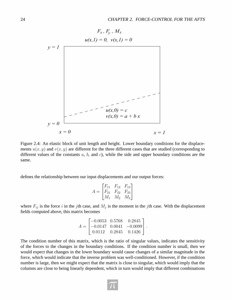
For the three different cases, we chose three different lower boundary conditions. See Figure 2.4. Inthe first case, we choose u(x, 0) = c and v(x, 0) = 0, where c is some constant. This case correspondsto pure shear in the x direction. For the second case, we consider pure compression in the positive ydirection, i.e., we have u(x, 0) = 0 and v(x, 0) = a, where a is some constant. In the third case, wetake u(x, 0) = 0 and v(x, 0) = bx, where b is some constant, which corresponds to a lower boundarythat ramps linearly from zero compression at x = 0 to a maximum compression at x = 1. Any linearcondition on the displacements at the lower boundary can be represented as linear combinations ofthese three input displacements.
We solve this system of partial differential equations (2.2–2.3) numerically using finite differenceson a 50 × 50 grid. We choose the constants λ = 1, µ = 1/2, a = 0.5, b = 0.5, and c = 0.5.
Once the displacements have been found, the forces and moment can be calculated using
Fy =
∫(
(λ+ 2µ)∂v
∂y+ λ
∂u
∂x
)
dx (normal) (2.5)
Fx =
∫
µ
(
∂u
∂y+∂v
∂x
)
dx (shear) (2.6)
M =
∫
x
(
(λ+ 2µ)∂v
∂y+ λ
∂u
∂x
)
dx (moment). (2.7)
We are interested in the values for these forces at the upper boundary (y = 1). We denote the normalforce at the upper boundary as F1, the stress along the upper boundary as F2, and the moment as M ,and calculate each of these for each of the three boundary conditions. We obtain a 3 × 3 matrix that
π
24 CHAPTER 2. FORCE-CONTROL FOR THE AFTS
x = 0 x = 1
y = 0
y = 1
u(x,0) = c
v(x,0) = a + b x
u(x,1) = 0, v(x,1) = 0
F , F , M yx x
Figure 2.4: An elastic block of unit length and height. Lower boundary conditions for the displace-ments u(x, y) and v(x, y) are different for the three different cases that are studied (corresponding todifferent values of the constants a, b, and c), while the side and upper boundary conditions are thesame.
defines the relationship between our input displacements and our output forces:
A =
F11 F12 F13
F21 F22 F23
M1 M2 M3
where Fij is the force i in the jth case, and Mj is the moment in the jth case. With the displacementfields computed above, this matrix becomes
A =
−0.0053 0.5768 0.2845−0.0147 0.0041 −0.00990.0112 0.2845 0.1426
.
The condition number of this matrix, which is the ratio of singular values, indicates the sensitivityof the forces to the changes in the boundary conditions. If the condition number is small, then wewould expect that changes in the lower boundary would cause changes of a similar magnitude in theforce, which would indicate that the inverse problem was well-conditioned. However, if the conditionnumber is large, then we might expect that the matrix is close to singular, which would imply that thecolumns are close to being linearly dependent, which in turn would imply that different combinations
π
2.5. MOVEMENT PATH PARAMETERIZATION 25
of inputs would produce very similar outputs. That is, the forces are not very sensitive to changes inthe lower boundary, and thus, the inverse problem is not very well conditioned.
The condition number for the matrix A is given by
cond(A) = 147.7,
indicating that the forces are not very sensitive to changes in the lower boundary. This can be seenmore clearly in Figure 2.5, in which the forces (represented by the three plots on the right side of thefigure) generated by variation of the lower boundaries conditions (shown on the left of the figure) arepresented on the same plot. It can be seen that even large differences in the lower boundary conditionscan result in only small changes in the forces.
This example provides evidence regarding the difficulty that may be involved in attempting todetermine the lower boundary conditions given the forces at the upper boundary. That is, the inverseproblem may not be well-conditioned. In such cases, finding solutions becomes difficult. Iterativemethods tend to converge slowly, and it is possible that they may not converge at all.
However, these results depend on the specific choices of the parameters of the problem λ and µ.Because we did not know the actual values of these parameters for the shoe, reasonable approximationswere chosen. Errors in this choice may affect the conclusions of this example.
Factors that effect the conditioning that we have not considered include the movement of the shoeon the prosthetic foot, which is expected to lead to poorer conditioning. Such movement would de-crease the sensitivity of the forces due to changes in the lower boundary, and thus increase the conditionnumber.
The zero displacement condition assumed at the top the prosthetic foot is almost certainly notsatisfied by the human foot and hence, no matter what continuum model is used for the foot-shoecombination, any attempt to examine the problem analytically will lead to different results for the twoproblems even if the displacement conditions at the shoe plate interface can be accurately reproduced.
2.5 Movement Path Parameterization
The evidence presented above indicates the difficulty involved in using closed-loop force control tosolve this problem. We, therefore, explore the possibility of non-locally controlling the forces along aparametrized movement path. It is expected that the conditioning of the inverse problem will still be anissue for this approach. However, variation of the parameters of the movement path would not lead tounnatural movements, which would reduce (perhaps eliminate) the need to make platform adjustmentsin directions that would cause unavoidable slipping. Because we did not have sufficient time duringthe workshop for a full investigation, we describe only briefly how one might go about using pathparametrization in this problem.
We begin by parameterizing the position data obtained from the human subject. We proceed bychoosing several points on the curves of each of the position variables. Examples for the spatialcoordinates are shown in Figure 2.6. The number and position of the points are chosen in such away as to maximize the reproduction of the qualitative features of the curves while minimizing thenumber of parameters needed. For example, for the z position data, it was judged that four points werenecessary to obtain a parametrized curve that could approximate both the sharp increase and decreasethat is observed at the beginning and end, respectively, of the time-series. After the points have been
π
26 CHAPTER 2. FORCE-CONTROL FOR THE AFTS
chosen, cubic spline interpolation can be used to obtain the parametrized approximation to each of thecurves.
For data acquired during the contact phase of a heel-toe run, the time-series of the six positionvariables could be reproduced reasonably well by fitting cubic splines to a total of 34 points. Theposition data for the 3 spatial coordinates is shown in Figure 2.6; data for the 3 angles is not shown.Thus, the path can be written as a function of the 34 parameters
Path = P (p1, p2, . . . , p34),
where pi are the path parameters that can be adjusted to vary the movement path. An example of howthe path might change when one of the parameters is varied is shown in Figure 2.7.
The forces can now be measured as the AFTS executes the initial parameterized path taken fromthe human subject data. That is, we have
Force = F (P ),
and we would like to find the 34 parameters pi that will reproduce the target force profile Ftarget. Inpractice, we will try to minimize some functional (e.g. with respect to the L2 norm) of the force andtarget force profiles over all possible parameter values. That is,
minP
‖Ftarget − F (P )‖2.
A standard method, perhaps a non-Jacobian method such as a polytope algorithm, might be used forthe minimization.
For the closed-loop force-control problem, we look for zeros of a function of six variables foreach interval along the path, whereas, here we are minimizing a single functional over 34 parameters.Although only one minimization problem needs to be solved, a large number of parameters are in-volved. The question arises whether such a method is feasible. Indeed, even if a Jacobian need not becalculated, a single ‘function evaluation’ consists of a full run of the AFTS, which took much longerthan one minute. It is not known how many such function evaluations would need to be executed todetermine the path parameters. However, it could possibly be in the hundreds. It is possible that a suf-ficient solution could be obtained by variation over only a smaller subset of the path parameters. Theseand other considerations require extensive further study before such a method could be implementedeffectively.
2.6 Conclusions
We would like to determine the particular movement path that would generate a specified target forceprofile. We examined the feasibility of performing a closed-loop control of the forces, and foundthat the nature of the problem does not lend itself well to this method. We do not conclude that it isimpossible to use closed-loop force control to solve the problem. However, the evidence indicates thatit would be very difficult to do so.
Parametrization of the movement path is one possible alternative. The promising feature of thismethod is that it would not lead to unnatural movements that could cause the shoe to slip along theplatform. Thus, it is expected that the reproducibility of force measurements would be significantly
π

2.6. CONCLUSIONS 27
improved. The conditioning of this method is not known; further study is required before conclusionsregarding the method’s feasibility can be made. Such investigations would require extensive dataacquisition using the AFTS itself.
Regardless of the method used, we discovered that it is necessary to reduce slipping of the shoealong the platform as much as possible. Simply resurfacing the platform may lead to significant im-provements in this respect. We also found that the platform will follow a different trajectory dependingon the origin of the platform coordinate system. Although the path differences are small, significantcumulative errors may arise. Thus, it would be prudent to ensure that the platform origin does not varyfrom run to run.
π
28 CHAPTER 2. FORCE-CONTROL FOR THE AFTS
0 10
0.5
1c
0 10
0.2
0.4shear
0 1−1
−0.5
0a
0 10
0.1
0.2b 0 1
0
0.1
0.2normal
0 1−0.04
−0.02
0moment
Figure 2.5: The two curves in the left panels represent two different sets of boundary conditions, i.e.of the constants a and b representing the amount of compression at the bottom boundary and slope ofthe bottom boundary, respectively, where the y-axis gives the values of the constants and the x-axisrepresents a parametrization for the changes in the constants. The curves in the right panels show theresulting differences in the forces, i.e., large changes in the boundary conditions only result in smallchanges in the forces, where the y-axis gives the values of the forces and the x-axis represents thesame parametrization as in the left panels.
π
2.6. CONCLUSIONS 29
0 5 10 15 20 25 30 35−120
−100
−80
−60
−40
−20
0
20
40
60
80
data point
X−Y−Z poisition of heel−toe run (human subject)
X
Y
Z
Figure 2.6: Position data in the x, y, and z directions for a heel-toe run of a human subject. Pointsalong the curves (the circles) have been chosen such that spline interpolants through these points willreasonably reproduce the curves.
π
30 CHAPTER 2. FORCE-CONTROL FOR THE AFTS
0 5 10 15 20 25 30 35−120
−100
−80
−60
−40
−20
0
20
40
60
80Spline Interpolants
X−Spline
Y−Spline
Z−Spline
Figure 2.7: Spline interpolants of the points taken from the x, y, and z position data of a heel-toe runof a human subject, as shown in Figure 2.6. Variation of one of the points represents how the path canchange as the path parameters are varied.
π

Chapter 3
Seismic Image Analysis Using Local Spectra
Problem presented by: Pierre Lemire & Rob Pinnegar (Calgary Scientific Inc.)
Mentors: Elena Braverman (University of Calgary), Michael Lamoureux (University of Calgary),Qiao Sun (University of Calgary)
Student Participants: John Gonzalez (Northeastern University), Hui Huang (University of BritishColumbia), Parisa Jamali (University of Western Ontario), Yongwang Ma (University of Calgary),Hatesh Radia (University of Massachusetts at Lowell), Jihong Ren (University of British Columbia),Dallas Thomas (University of Lethbridge), Pengpeng Wang (Simon Fraser University)
Report prepared by: M. Lamoureux ([email protected])
3.1 Introduction
During the one week Industrial Problem Solving Workshop held in June 2005 at the University ofCalgary, hosted by the Pacific Institute for the Mathematical Sciences, our group was asked to considera problem in seismic imaging, as presented by researchers from Calgary Scientific Inc. The essenceof the problem was to understand how the S-transform could be used to create better seismic images,that would be useful in identifying possible hydrocarbon reservoirs in the earth.
3.2 Problem Description
Our group was presented with the following summary of the problem under consideration:
Calgary Scientific Inc. is currently developing a technique to classify pixels in seismicpseudosections based on their local spectral characteristics. These are obtained from amodified Gabor transform, in which only certain (kx, ky) wavevectors are representedin the local spectrum of each pixel. This classification technique involves finding thedominant peak in each local spectrum, and identifying the corresponding pixel with thewavevector and amplitude of the dominant peak.
31
32 CHAPTER 3. SEISMIC IMAGE ANALYSIS USING LOCAL SPECTRA
This method proved ineffective since it is inflexible when one wants to investigate any in-teresting features not associated with the dominant peak. The identification of secondarypeaks is complicated by the fact that dominant peaks typically cover several pixels of itslocal spectrum; hence, the wavevector with the second largest amplitude is likely to con-tain a significant contribution from the primary peak. The main goals were to efficientlyidentify secondary peaks and to identify correlations amongst peaks from pixel to pixel.
Ideally, a fully processed seismic pseudosection should contain all the information theinterpreter needs to unambiguously identify potential drilling targets, such as reefs, anti-cline traps, and so forth. This involves identifying layer boundaries on the pseudosection,a process that can be considered as more or less equivalent to identifying the layers them-selves as continuous groups of pixels. The presence of significant amounts of noise in thedata, and the accumulation of errors during the numerical steps of seismic processing, cancomplicate this process by obscuring important features in the pseudosection. A final goalis to improve the signal to noise ratio to facilitate interpretation of the pseudosection.
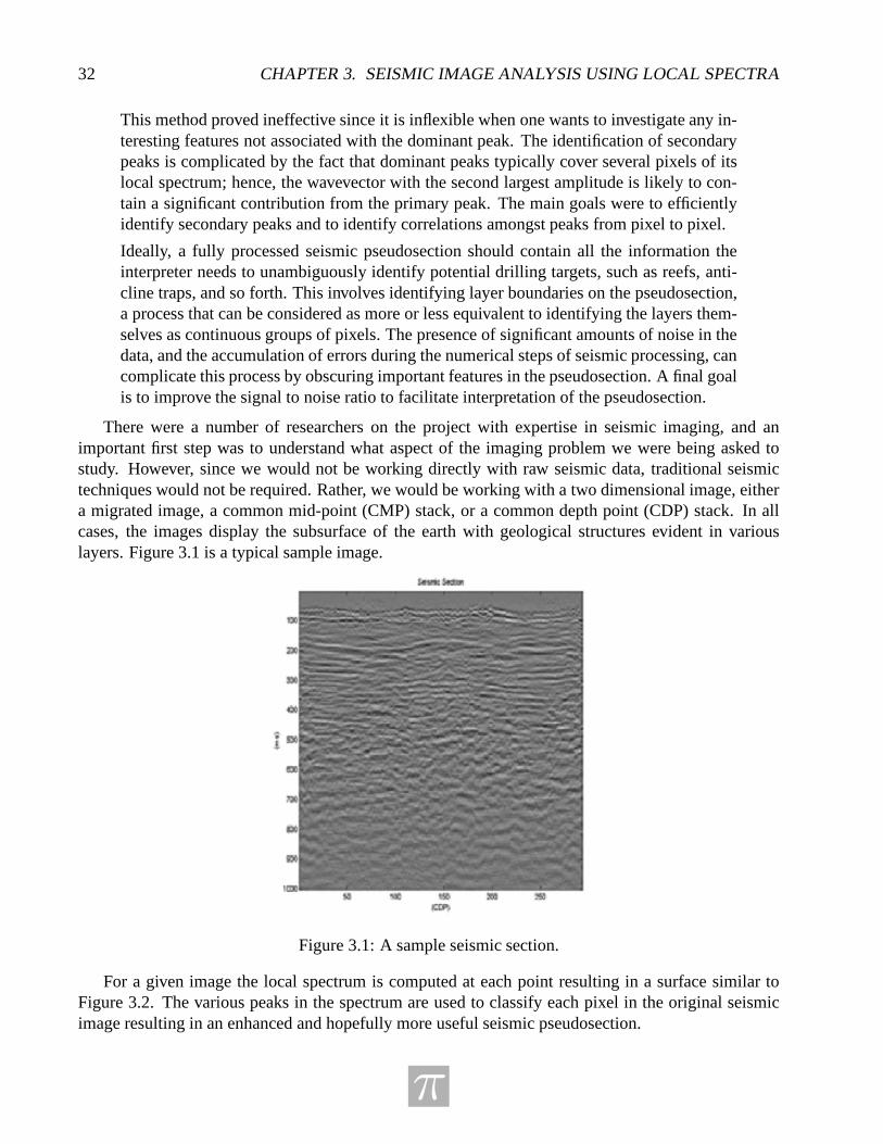
There were a number of researchers on the project with expertise in seismic imaging, and animportant first step was to understand what aspect of the imaging problem we were being asked tostudy. However, since we would not be working directly with raw seismic data, traditional seismictechniques would not be required. Rather, we would be working with a two dimensional image, eithera migrated image, a common mid-point (CMP) stack, or a common depth point (CDP) stack. In allcases, the images display the subsurface of the earth with geological structures evident in variouslayers. Figure 3.1 is a typical sample image.
Figure 3.1: A sample seismic section.
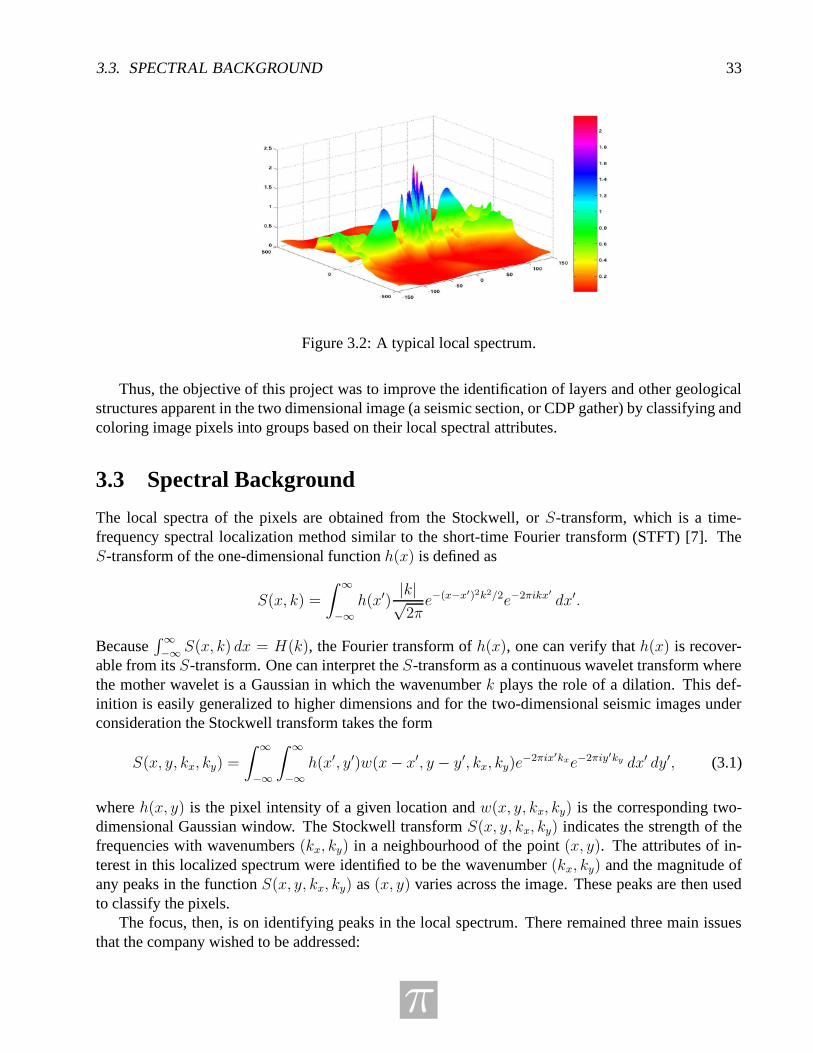
For a given image the local spectrum is computed at each point resulting in a surface similar toFigure 3.2. The various peaks in the spectrum are used to classify each pixel in the original seismicimage resulting in an enhanced and hopefully more useful seismic pseudosection.
π
3.3. SPECTRAL BACKGROUND 33
Figure 3.2: A typical local spectrum.
Thus, the objective of this project was to improve the identification of layers and other geologicalstructures apparent in the two dimensional image (a seismic section, or CDP gather) by classifying andcoloring image pixels into groups based on their local spectral attributes.
3.3 Spectral Background
The local spectra of the pixels are obtained from the Stockwell, or S-transform, which is a time-frequency spectral localization method similar to the short-time Fourier transform (STFT) [7]. TheS-transform of the one-dimensional function h(x) is defined as
S(x, k) =
∫
∞
−∞
h(x′)|k|√2πe−(x−x′)2k2/2e−2πikx′
dx′.
Because∫
∞
−∞S(x, k) dx = H(k), the Fourier transform of h(x), one can verify that h(x) is recover-
able from its S-transform. One can interpret the S-transform as a continuous wavelet transform wherethe mother wavelet is a Gaussian in which the wavenumber k plays the role of a dilation. This def-inition is easily generalized to higher dimensions and for the two-dimensional seismic images underconsideration the Stockwell transform takes the form
S(x, y, kx, ky) =
∫
∞
−∞
∫
∞
−∞
h(x′, y′)w(x− x′, y − y′, kx, ky)e−2πix′kxe−2πiy′ky dx′ dy′, (3.1)
where h(x, y) is the pixel intensity of a given location and w(x, y, kx, ky) is the corresponding two-dimensional Gaussian window. The Stockwell transform S(x, y, kx, ky) indicates the strength of thefrequencies with wavenumbers (kx, ky) in a neighbourhood of the point (x, y). The attributes of in-terest in this localized spectrum were identified to be the wavenumber (kx, ky) and the magnitude ofany peaks in the function S(x, y, kx, ky) as (x, y) varies across the image. These peaks are then usedto classify the pixels.
The focus, then, is on identifying peaks in the local spectrum. There remained three main issuesthat the company wished to be addressed:
π

34 CHAPTER 3. SEISMIC IMAGE ANALYSIS USING LOCAL SPECTRA
1. In Calgary Scientific’s current algorithm, the four-dimensionalS-transform is collapsed to a two-dimensional image by identifying each pixel with the wavevector at which its local S-spectrum islargest. That is, one particular peak is identified. This approach assumes that only one waveformis important at any pixel in the image.
2. A reliable means of automated edge detection is elusive. Although the approach described abovecan be used to produce a visually interpretable pseudo-image, it cannot be used to divide theimage into layers because the peak wavevector can vary from pixel to pixel within a particularlayer.
3. In Calgary Scientific’s implementation, the S-transform is evaluated at a set of positions {(x, y)}which changes as the wavevectors change. This complicates any pattern matching because thelocal S-spectra of adjacent (x, y) pixels are typically not defined on the same set of wavevectors.There are some standard techniques to account for this but they all introduce artifacts in thetransformation. Is there a better way to compute the transform at all interesting positions (x, y)and wavenumbers (kx, ky)?
3.4 Addressing Issue One: Identifying Spectral Peaks
In the sample data sets that we considered, the spectral peaks were all remarkably smooth, andGaussian-like. Whether this was a property of the data, or a property of the S-transform was notinvestigated in detail. However, it appears that it is a reflection of the redundancy in the S-transform.The smoothness, and Gaussian shape, suggested a number of approaches for identifying peaks. Asummary of the ones we considered were:
• Reduce the two-dimensional peak selection problem to a series of one-dimensional problems.Using the slicing technique, we can consider all one-dimensional sections of the spectrum andanalyze the peak structure of each slice. From this we identify the peaks of the entire spectrum.In the one-dimensional slice, the spectrum appears smooth enough (twice differentiable), to findand classify all the maxima.
• Use a discrete, derivative to find critical points, and identify peaks. Since the function is smooth,this technique should rapidly identify the few peaks there are. Ranking them by height is simple.
• Represent the function as a sum of Gaussians and use a least squares technique to specify theirindividual parameters. After that, the highest peaks are easily classified.
• Identify the highest peak and subtract an appropriate Gaussian-like function centered at thispeak. After the subtraction, find the highest peak and repeat the procedure. It was believed thatthis could expose high peaks shadowed by adjacent higher peaks.
• Use clustering techniques to group the data around peaks, thus dividing all the data into severalgroups associated with various peaks. Later these groups can be ranged in accordance to thepeak values.
π
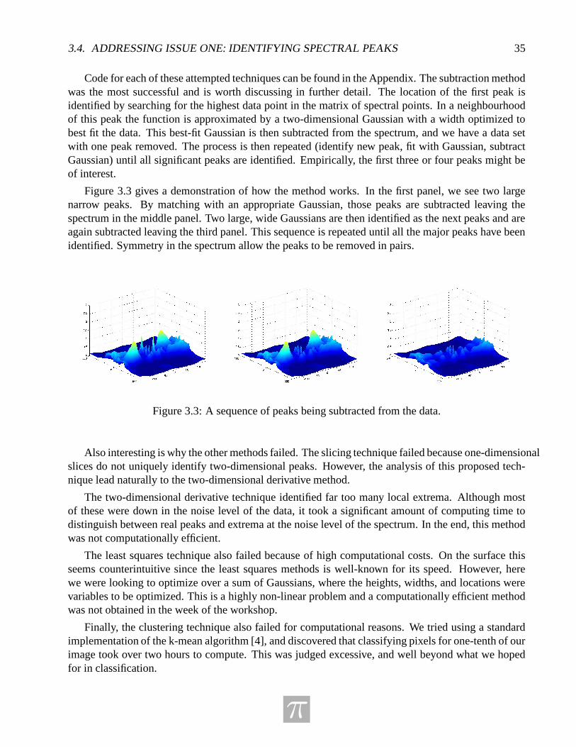
3.4. ADDRESSING ISSUE ONE: IDENTIFYING SPECTRAL PEAKS 35
Code for each of these attempted techniques can be found in the Appendix. The subtraction methodwas the most successful and is worth discussing in further detail. The location of the first peak isidentified by searching for the highest data point in the matrix of spectral points. In a neighbourhoodof this peak the function is approximated by a two-dimensional Gaussian with a width optimized tobest fit the data. This best-fit Gaussian is then subtracted from the spectrum, and we have a data setwith one peak removed. The process is then repeated (identify new peak, fit with Gaussian, subtractGaussian) until all significant peaks are identified. Empirically, the first three or four peaks might beof interest.
Figure 3.3 gives a demonstration of how the method works. In the first panel, we see two largenarrow peaks. By matching with an appropriate Gaussian, those peaks are subtracted leaving thespectrum in the middle panel. Two large, wide Gaussians are then identified as the next peaks and areagain subtracted leaving the third panel. This sequence is repeated until all the major peaks have beenidentified. Symmetry in the spectrum allow the peaks to be removed in pairs.
Figure 3.3: A sequence of peaks being subtracted from the data.
Also interesting is why the other methods failed. The slicing technique failed because one-dimensionalslices do not uniquely identify two-dimensional peaks. However, the analysis of this proposed tech-nique lead naturally to the two-dimensional derivative method.
The two-dimensional derivative technique identified far too many local extrema. Although mostof these were down in the noise level of the data, it took a significant amount of computing time todistinguish between real peaks and extrema at the noise level of the spectrum. In the end, this methodwas not computationally efficient.
The least squares technique also failed because of high computational costs. On the surface thisseems counterintuitive since the least squares methods is well-known for its speed. However, herewe were looking to optimize over a sum of Gaussians, where the heights, widths, and locations werevariables to be optimized. This is a highly non-linear problem and a computationally efficient methodwas not obtained in the week of the workshop.
Finally, the clustering technique also failed for computational reasons. We tried using a standardimplementation of the k-mean algorithm [4], and discovered that classifying pixels for one-tenth of ourimage took over two hours to compute. This was judged excessive, and well beyond what we hopedfor in classification.
π
36 CHAPTER 3. SEISMIC IMAGE ANALYSIS USING LOCAL SPECTRA
3.5 Addressing Issue Two: Edge Detection
The idea here is that near a linear feature in the original two-dimensional image, such as along anedge, the local spectra should not vary much from pixel to pixel. Consequently, it should be possibleto identify correlations between spectral peaks as one moves from pixel to pixel. To test this idea,one can begin with the peak identification algorithm in Section 3.4, and apply some statistical tests forcorrelations.
Unfortunately, one week was not long enough to allow us to get both the peak detection algorithmworking and statistically analyse the results. A larger database of seismic images and correspondingS-transforms would be required to pursue this avenue of research.
It is worth noting that the local spectral information of the S-transform varies slowly from pixelto pixel, so there should be quite a high level of correlation. What is required is a statistical test thatcan distinguish correlations that come from data with those that are merely a reflection of the slowlychanging nature of the S-transform.
There were also suggestions to use some alternatives of S-transform. In particular, the applicationof methods which identify local spectra not at each individual pixel but from a group of adjacent pixels.Some adaptive methods were proposed as follows:
• The localized Fourier method. This method also has an adaptive version which can be appliedto various time grids.
• Certain wavelet-like techniques for directional analysis, such as brushlets, ridgelets, or curvelets [8].These wavelet bases were originally developed for directional image processing and identifyingslanted patterns. Such techniques seem directly applicable to these seismic images.
3.6 Addressing Issue Three: Computing the S-transform
This was probably the most challenging issue to address. A direct implementation of the S-transformis highly redundant and leads to a massive amount of data, as each data point is transformed into a fullspectrum. For instance, a simple 100 by 100 image transforms into 100 million data points (100 ×100)2. The company does have some impressively fast algorithms for computing an approximation tothe complete transform, but with this level of redundancy, the question must be asked: are there betterapproaches? We did not have access to their implementation of the algorithm, so direct investigationof how it was implemented, or how it could be improved, were not possible. Some possible ideas topursue include:
• compute a sparse subset of the transform and apply interpolation for the intermediate points;
• compute a sparse subset of the transform and use this directly to estimate peaks;
• investigate if an analog of a fast transform (FFT, wavelet, etc.) could be applied to the S-transform. In particular, the S-transform looks very similar to a phase-shifted continuous wavelettransform, so there may be some close connections to the wavelet speedup;
• consider using a different transform, such as the Gabor or wavelet transforms, which also pro-duce local spectral information, but have a fast implementation.
π

3.7. ADDITIONAL ISSUES: STEPPING BACK TO SEISMIC 37
Unfortunately, we did not have time to investigate these approaches in detail.
3.7 Additional Issues: Stepping Back to Seismic
In the end, this problem is really about seismic data imaging and analysis. It is important to realizethat in all the images so created, there are the important physical aspects that should be properlymodelled. That is, the images come from seismic experiments involving wave propagation; errorsin the image come from errors in our physical model; the geological structures we hope to identifycome from physical processes such as sedimentary deposition, geological faulting, and so on. It isa bit frustrating to begin the mathematical analysis at the end of the data processing, where we havean image that came from somewhere, and we want to analyse it. With sufficient mathematical andcomputational tools, it makes sense to go back to the original seismic data, and apply our researchtechniques to understand how this raw data can be used to reveal more accurately the features we seekto identify. This is a big task, not easily accomplished in a week-long problem solving workshop. Aninterested reader could refer to the work of the POTSI project (potsi.math.ucalgary.ca) orthe CREWES project (www.crewes.org) for further information on research in the mathematicsand geophysics of seismic imaging.
3.8 Acknowledgments
We thank Peirre Lemire and Rob Pinnegar of Calgary Scientific Inc. for all their help and guidanceduring our weeklong project. We also thank the Pacific Institute for Mathematical Sciences for theirsupport of the Industrial Problem Solving Workshop.
3.9 Appendix
We include here some of our key MATLAB routines.
The main script for identifying peaks, in 2D and 3D
% PIXEL -- A script program for picking-up peaks in a local spectrum% created by the S-Transforms and removing them%% By Yongwang Ma% University of Calgary, Alberta, Canada% May 20, 2005%% You may copy, modify and distribute the codes for purpose of% research.%
% process and plot in 2D
π

38 CHAPTER 3. SEISMIC IMAGE ANALYSIS USING LOCAL SPECTRA
load SH02_LocalSpec_117_177.mat;dimension = 2;npick = 10; % number of pairs of peaks to remove[F,nmovie] = pick(LocalSpec,npick,dimension);
% process and plot in 3D
load SH02_LocalSpec_117_177.mat;dimension = 3;npick = 10; % number of pairs of peaks to remove[F,nmovie] = pick(LocalSpec,npick,dimension);
The subtractional subroutine
function [F,nmovie] = pick(SparseLS,npick,dimension)% pick - finds peaks and creates humps (gaussian-like function in 2D)% in an image (spectrum) and substracts it from the original image%% By Yongwang Ma, May 18, 2005% The University of Calgary% Calgary, Alberta, Canada%% Input:% SparseLS = input image, a matrix% npick = the number of pairs of peaks needs to be found% dimension = dimension of final images (2- 2D images; 3-3D images)%% Output:% F = a structure consisting of parameters of the frames for a movie% nmovies = a vector storing the order of the images (figures)
pix_mat = SparseLS;NF_half = floor(size(pix_mat,1)/2);NK_half = floor(size(pix_mat,2)/2);f = [-NF_half:NF_half];k = [-NK_half:NK_half];M = size(pix_mat,1);N = size(pix_mat,2);sig = 1.50; % parameter controlling the width of Gaussian-like windowfigure; % using only one figure, so finally only the most updated image is shownfor ipeak = 1:npick
pmax = max(max(pix_mat));% find the position of maximum (peak) in the spectrum
π

3.9. APPENDIX 39
for m = 1:Mfor n = 1:N
temp = pix_mat(m,n);if (temp == pmax)
f0 = m; k0 = n;end
endend% record the coordinates of peaks identifiedfpeak(ipeak) = f0;kpeak(ipeak) = k0;% transform the coordinatesif (f0 >= NF_half)
f_0 = f0-NF_half;else
f_0 = -(NF_half-f0);endif (k0 >= NK_half)
k_0 = k0-NK_half;else
k_0 = -(NK_half-k0);endf_01 = - f_0;k_01 = -k_0;gaus_p = gaus1(f_0,k_0,M,N,k,f,sig);gaus_p1 = gaus1(f_01,k_01,M,N,k,f,sig);sub_pmat = pix_mat-gaus_p.*pix_mat;sub_pmat1 = sub_pmat-gaus_p1.*sub_pmat;
% Plot out results of pickingif (dimension ==2)
%figure;imagesc(sub_pmat1);
else % (3D)%figure;surf(k,f,sub_pmat1);axis([k(1) k(end) f(1) f(end) 0 3])shading flat
endif ipeak==1
boundz=get(gca,’CLim’);endset(gca,’CLim’,boundz);
% figure;imagesc(gaus_p);
π

40 CHAPTER 3. SEISMIC IMAGE ANALYSIS USING LOCAL SPECTRA
% figure;% amat=gaus_p.*pix_mat;% plot(amat(f0,:));% hold;% plot(pix_mat(f0,:));% plot(sub_pmat(f0,:));
pix_mat = sub_pmat1;F(ipeak) = getframe;
end% create a movienmovie = zeros(1,24*npick);nrmovie = zeros(1,24*npick);nn1 = 1;nn2 = 24;nnr1 = 24*npick;nnr2 = 24*(npick-1)+1;for in = 1:npick
nmovie(1,nn1:nn2) = in;nrmovie(1,nnr1:-1:nnr2) = in;nn1 = nn1+24;nn2 = nn2 + 24;nnr1 = nnr1-24;nnr2 = nnr2-24;
end%play the movie forwardsmovie(F,nmovie);% play the movie backwards% movie(F,nrmovie);
The subroutine to compute the Gaussian-like function
function gaus = gaus1(f0,k0,M,N,k,f,sig)
% gaus1 = subroutine to calculate a gaussian_like function (2D)%% f0 = frequency, coordinate at which the centre of gaussian-like function% located% k0 = wavenumber, coordinate at which the centre of gaussian-like% funcition located% M = total number of frequency samples% N = totlal number of wavenumber samples% k = wavenumber coordinates, a row vector% f = frequency coordinates, a row vector% sig = a factor, which determines the width of the gaussian-like function
π

3.9. APPENDIX 41
p11 = zeros(M,N);p22 = zeros(M,N);stab = 1.e-8; % stability factorfor m = 1:M
p11(m,:) = (f(m)-f0).ˆ2/Mˆ2+(k-k0).ˆ2/Nˆ2;p22(m,:) = (f(m)/M)ˆ2 + (k/N).ˆ2;
endgaus = exp(-2*piˆ2*(p11./(p22+stab))/(sigˆ2));
π

42 CHAPTER 3. SEISMIC IMAGE ANALYSIS USING LOCAL SPECTRA
π

Bibliography
[1] Aki, K. & Richards, P.G. (2002). Quantitative Seismology (2nd edition). University Science Book:Sausilito.
[2] Averbuch, A.Z., Meyer, F.G., Stromberg, J.O., Coifman, R.R. & Vassiliou, A. (2001). Low Bit-Rate Efficient Compression for Seismic Data. IEEE Transactions on Image Processing, 10(12), pp.1801-1814.
[3] Coifman R.R. & Meyer, Y. (1991). Remarques sur l’analyse de Fourier a fenetre. Comptes Rendusde l’Academie des Sciences, Serie I, 312(3), pp. 259-261.
[4] MacQueen, J.B. (1967). Some methods for classification and analysis of multivariate observations.In Proceedings of the Fifth Berkeley Symposium on Mathematical Statistics and Probability. VolI, Statistics. Edited by Lucien M. Le Cam and Jerzy Neyman. University of California Press, pp.281-297.
[5] Meyer F.G. & Coifman, R.R. (1997). Brushlets: a tool for directional image analysis and imagecompression. Applied and Computational Harmonic Analysis, 4, pp. 147-187.
[6] Press, W.H., Flannery, B.P., Teukolsky, S.A. & Vettering, W.T. (1992). Numerical Recipes in C(2nd edition). Cambridge University Press: Cambridge.
[7] Stockwell, R.G., Mansinha, L. & Lowe, R.P. (1996). Localization of the Complex Spectrum: TheS Transform. IEEE Transactions on Signal Processing, 44(4), pp. 998-1001.
[8] Welland, G.V. (2003). Studies in Computational Mathematics, Vol 10: Beyond Wavelets. Aca-demic Press.
43

44 BIBLIOGRAPHY
π
Chapter 4
Adaptive Statistical Evaluation Tools forEquity Ranking Models
Problem presented by: Brad Bondy (Genus Capital Management)
Mentors: Tony Ware (University of Calgary), Len Bos (University of Calgary)
Student Participants: Amir Amiraslani (University of Western Ontario), Thomas Holloway (Uni-versity of Alberta), Hua Li (University of Calgary), Maryam Mizani (University of Victoria), Mah-yar Mohajer (University of Calgary), Comron Nouri (University of Western Ontario), Gergeli Orosi(University of Calgary), Nargol Rezvani (University of Western Ontario), Liang Xu (University ofWashington), Oulu Xu (York University)
Report prepared by: Tony Ware ([email protected])
4.1 Introduction
Based in Vancouver, Genus Capital Management (http://www.genuscap.com) is an indepen-dent investment provider who for over 15 years have been managing assets for private individuals andfamilies, trusts, foundations and pension funds from across Canada. Their investments span a range ofequity and fixed income, and they manage assets to the value of about $1.3-billion.
Genus offer investment portfolios with a variety of flavours. Each portfolio consists of investmentsin stocks from some given ‘universe’. Competitive advantage comes from consistently out-performingcompeting funds. One of the approaches that Genus use to achieve competitive advantage is to makeuse of auxiliary information about the stocks in the universe in deciding how to adjust their portfoliomonth by month. The problem that Genus brought to the IPSW was concerned with how to improvethe way this information is utilised.
4.2 Problem Description
A major challenge in the investment management business is to identify which stocks are likely tooutperform in the future, and which are likely to perform relatively poorly. To this end the strategy
45

46 CHAPTER 4. EVALUATION OF EQUITY RANKING MODELS
adopted by Genus is to identify factors (auxiliary information about the stock such as earnings-to-priceratio or dividend yield) that they believe are associated with future out-performance (i.e. factors thathave predictive ability). The best of these factors are then combined (Genus use a weighted average)into a model which is used to rank the universe of stocks month-by-month. This ranking is then usedto as the input to a trading strategy, resulting in a modified portfolio.
A critical step in this process is to identify the ‘good’ factors and to determine how heavily eachshould be weighted in the final model. Currently Genus use in-sample back-tests in which they sim-ulate a trading strategy of, for example, selling stocks that drop below the 40th percentile (of theranking) and reinvesting the proceeds in stocks in the top 20th percentile. These simulations are runover a wide range of potential weighting schemes or models, and the model with the most attractiveattributes is identified. Attributes that Genus typically look for in a model include:
• High spread between returns for top and bottom quintiles.
• High information ratio: the ratio of the mean and standard deviation of the excess monthly returnon portfolio versus the index (a portfolio in which all the stocks in the universe are equally-weighted).
• High hit ratio: the percentage of months in which the portfolio outperforms the index.
The in-sample back-tests are typically run over a 10-year period, excluding the most recent 2 years.Once a model is identified, out-of-sample tests of the model over the most recent 2 years are run inorder to ensure that the model works out-of-sample.
A major issue for Genus is the inflexibility that results from the 2-year delay for out-of-sampletesting. Factors tend to lose their predictive ability as other market participants incorporate them, anduseful new factors seem to be getting cleaned out faster and faster. With the 2-year delay Genus runthe risk of delaying introduction of a new factor until the market has already cleaned it out. On theother hand, if the out-of-sample tests are eliminated, they run the risk of over-fitting the data.
The challenge posed for the workshop team was:
1. to recommend adaptive statistical evaluation tools (alternatives to out-of-sample tests) that couldbe used to improve confidence in a model and to help decide in a timely fashion if a new factorshould be added to a model, or if an existing factor should be removed;
2. to suggest algorithms that could be used to dynamically update the models with a view to ex-ploring a dynamic strategy in which model factors and weights are updated monthly based onthe evaluation measures.
4.3 Rising to the Challenge
It was clear from the outset that if the team were to be able to address either of these challenges real-istically they would need to build tools that would enable them to implement the various componentsof Genus’ portfolio management strategy. As the week progressed, it became apparent that a majorstumbling block would be implementation of an efficient procedure for finding a ‘good’ model forranking the stocks. This became the focus of the team’s efforts.
π

4.3. RISING TO THE CHALLENGE 47
Genus had provided the team with sample data, consisting of just over 12 years worth of monthlyreturns on a universe of 60 stocks, along with time series of 34 factors for each of the stocks. Usingthese data, the approach was to build software (MATLAB) models for:
• ranking the stocks based on factor information;
• implementing a trading strategy based on a stock ranking and assessing the performance of agiven trading strategy by looking at measures such as hit ratio, information ratio and spread.
The IPSW team implemented a simplified trading strategy of selling the entire portfolio each month,and using the proceeds to invest equally in the top 20% of stocks as given by the computed ranking.They also implemented the following measures of portfolio performance: excess return, hit ratio andinformation ratio.
4.3.1 Ranking
As noted above, determining an an effective procedure for ranking the stocks is a critical step, but thedesign of such a procedure cannot be separated from the other tasks, and in particular the choice oftrading strategy, or performance assessment measures.
A simplified description of the approach taken by Genus is the following. Given a set of factorvalues fi,j(t) for the jth factor corresponding to ith stock at time t, and given a linear weighting vector~w = (wj), they produce a ranking at each time t from the score vector
Si(t;w) :=∑
j
wjfi,j(t).
A trading strategy, such as buying the top quintile of stocks (those obtaining the top 20% scores) inequal measure, is assumed (the actual strategy adopted by Genus is rather more complicated than this,but the details were not available to the IPSW team). The trading strategy takes the weighting vector~w and the factor values for a given date and produces a set of portfolio weights αi(t). The actual stockreturns Ri(t) can then be used to compute the portfolio return
∑
i
αi(t)Ri(t).
Given such a strategy, the performance of the model can be assessed by measuring the resulting excessportfolio returns, the information ratio, the hit ratio, and other parameters.
In order to determine a ‘good’ weighting vector ~w, Genus select a training period (typically a ten-year period of time excluding the most recent two years). They construct a grid of possible weightingvectors, spanning a subset of the total set of possibilities; for each vector in the grid they producerankings for each date in the training period, and (using the trading strategy) compute the correspond-ing portfolio excess returns, hit ratios, information ratios, etc. They then select the best-performingweighting vector from this sample and test it against the most recent two-year period before putting itto use.
The determination of a ranking model is an optimisation problem, with a highly nonlinear objectivefunction (irrespective of which of the portfolio measures is used). The IPSW team decided that therecould be significant advantages to be gained from exploring alternative approaches to the design of op-timal ranking algorithms. They considered three distinct techniques: a genetic optimisation algorithm,a neural network, and a constrained least-squares approach.
π
48 CHAPTER 4. EVALUATION OF EQUITY RANKING MODELS
4.3.2 Genetic Optimization
Genetic optimization is an evolutionary search technique (see [2] for more information), in which apopulation of abstract representations of candidate solutions (individuals) evolves towards better so-lutions. The evolution begins with a population of randomly selected individuals and proceeds ingenerations. The transition from generation to generation involves evaluating the fitness of the cur-rent population; individuals are randomly selected for reproduction (with a probability based on theirfitness). Individuals selected for reproduction are randomly selected for mating (each pair producestwo offspring, each of which has some combination of the features of their parents). In addition, eachfeature of the offspring can mutate independently with a given probability.
Parameters and Results
Genetic optimisation was used to search for an optimum weight vector ~w for use in a linear rankingmodel as described above. The first 113 months of factor and return data were used to construct theobjective function, which took a weighting vector as input and gave the resulting excess returns as out-put. The populations consisted of 30 individuals, with a 0.01 probability of mutation of the offspringfeatures, and the algorithm was allowed to evolve for 1000 generations before being terminated. Theresulting weight vector ~w0 is shown in Figure 4.1.
In Figure 4.2, the objective function in the neighbourhood of ~w0 is illustrated. Each of the graphsin the figure depicts a ‘slice’ of the objective function in the direction of one of the 34 coordinatedirections, centred at ~w0. The non-smooth nature of the objective function can be readily seen, as isthe fact that the genetic algorithm has attained something close to, but not exactly at, a maximum.
4.3.3 Neural Network
An artificial neural network (see [3] for more information) is a computational model for informationprocessing, represented by a nonlinear function ν that maps a vector of input values ~x to a vector ofoutput values ~y. The nonlinear function has a particular form given by a network structure togetherwith weights associated with the network connections. A feed forward network typically has an inputlayer, with a node for each element of ~x, an output layer, with a node for each element of ~y, and one ormore hidden layers in between. Each node in a given layer can be connected to each node in the nextlayer.
The nodes in the input layer do no processing: they simply pass on the input values to the nodes inthe next layer to which they are connected.
Nodes in the hidden layers receive values from the incoming connections; they process these valuesin some way before determining a value to pass on to the nodes in the next layer. A common choicefor computing the output value is to compute a weighted linear combination of the inputs (the weightsbeing those associated with the incoming connections) and to apply a logistic function, for exampleψ(s) = 1
1+e−s , to the result. Nodes in the output layer compute the elements of the vector ~y bycomputing the weighted combination of their inputs. A network of this sort is an example of a multi-layer perceptron.
Even with just one hidden layer, such a network has a universal approximation property, and can—with an appropriate choice of connection weights—reproduce arbitrarily closely the action of anycontinuous function that maps intervals of real numbers to intervals of real numbers [1].
π
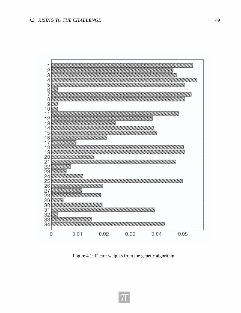
4.3. RISING TO THE CHALLENGE 49
Figure 4.1: Factor weights from the genetic algorithm.
π
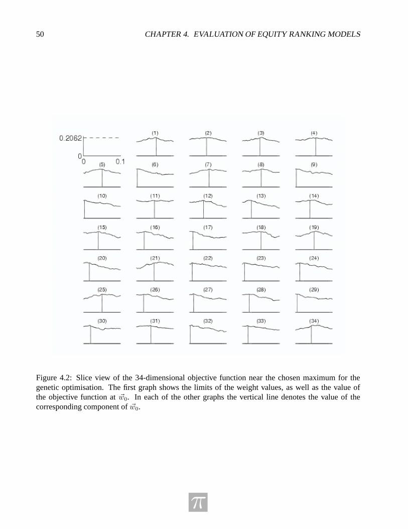
50 CHAPTER 4. EVALUATION OF EQUITY RANKING MODELS
Figure 4.2: Slice view of the 34-dimensional objective function near the chosen maximum for thegenetic optimisation. The first graph shows the limits of the weight values, as well as the value ofthe objective function at ~w0. In each of the other graphs the vertical line denotes the value of thecorresponding component of ~w0.
π
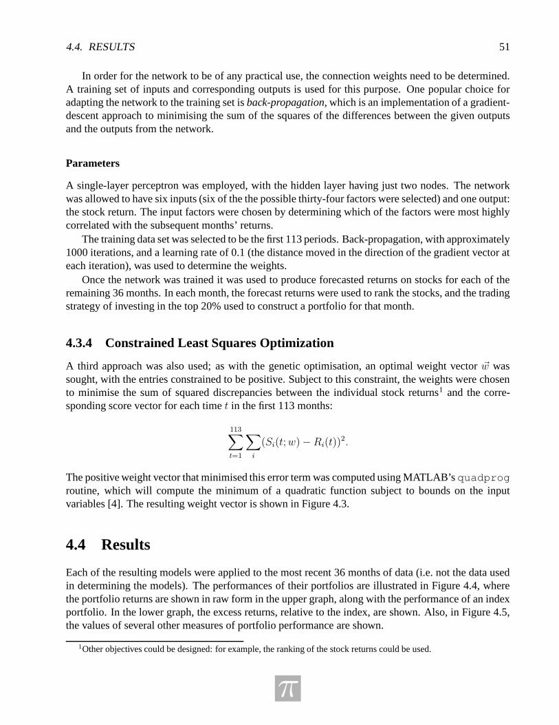
4.4. RESULTS 51
In order for the network to be of any practical use, the connection weights need to be determined.A training set of inputs and corresponding outputs is used for this purpose. One popular choice foradapting the network to the training set is back-propagation, which is an implementation of a gradient-descent approach to minimising the sum of the squares of the differences between the given outputsand the outputs from the network.
Parameters
A single-layer perceptron was employed, with the hidden layer having just two nodes. The networkwas allowed to have six inputs (six of the the possible thirty-four factors were selected) and one output:the stock return. The input factors were chosen by determining which of the factors were most highlycorrelated with the subsequent months’ returns.
The training data set was selected to be the first 113 periods. Back-propagation, with approximately1000 iterations, and a learning rate of 0.1 (the distance moved in the direction of the gradient vector ateach iteration), was used to determine the weights.
Once the network was trained it was used to produce forecasted returns on stocks for each of theremaining 36 months. In each month, the forecast returns were used to rank the stocks, and the tradingstrategy of investing in the top 20% used to construct a portfolio for that month.
4.3.4 Constrained Least Squares Optimization
A third approach was also used; as with the genetic optimisation, an optimal weight vector ~w wassought, with the entries constrained to be positive. Subject to this constraint, the weights were chosento minimise the sum of squared discrepancies between the individual stock returns1 and the corre-sponding score vector for each time t in the first 113 months:
113∑
t=1
∑
i
(Si(t;w) − Ri(t))2.
The positive weight vector that minimised this error term was computed using MATLAB’s quadprogroutine, which will compute the minimum of a quadratic function subject to bounds on the inputvariables [4]. The resulting weight vector is shown in Figure 4.3.
4.4 Results
Each of the resulting models were applied to the most recent 36 months of data (i.e. not the data usedin determining the models). The performances of their portfolios are illustrated in Figure 4.4, wherethe portfolio returns are shown in raw form in the upper graph, along with the performance of an indexportfolio. In the lower graph, the excess returns, relative to the index, are shown. Also, in Figure 4.5,the values of several other measures of portfolio performance are shown.
1Other objectives could be designed: for example, the ranking of the stock returns could be used.
π

52 CHAPTER 4. EVALUATION OF EQUITY RANKING MODELS
Figure 4.3: Factor weights from the constrained least squares optimisation.
π
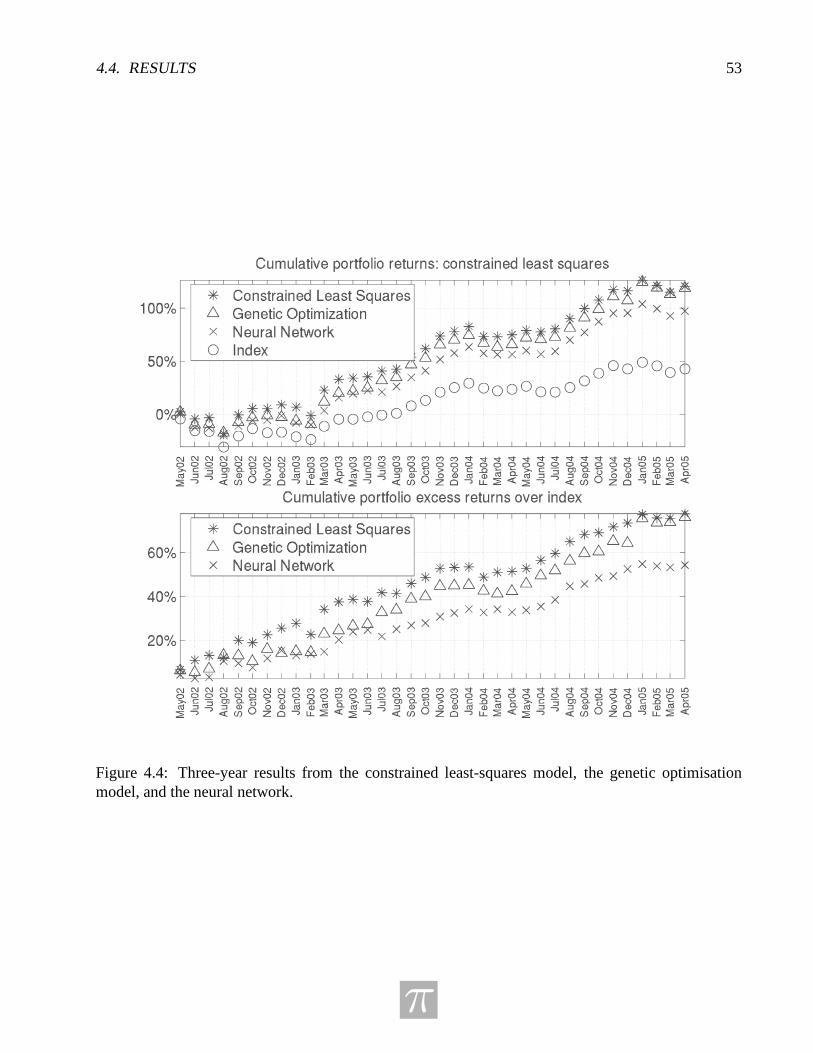
4.4. RESULTS 53
Figure 4.4: Three-year results from the constrained least-squares model, the genetic optimisationmodel, and the neural network.
π
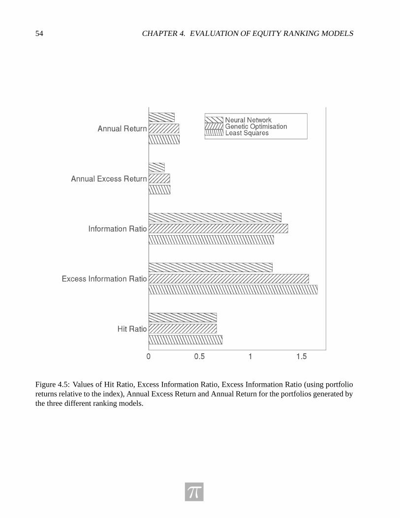
54 CHAPTER 4. EVALUATION OF EQUITY RANKING MODELS
Figure 4.5: Values of Hit Ratio, Excess Information Ratio, Excess Information Ratio (using portfolioreturns relative to the index), Annual Excess Return and Annual Return for the portfolios generated bythe three different ranking models.
π

4.5. CONCLUSIONS AND DIRECTIONS FOR FURTHER WORK 55
4.5 Conclusions and Directions for Further Work
The results from the three ranking models shown in the previous section are illustrative only. Each ofthe approaches is capable of refinement. However, the results obtained—even without refinement—compare well with the performance of Genus’ current model. Each of the approaches has the potentialto deliver significant improvements for Genus. Moreover, especially in the case of the constrainedleast-squares optimisation, they can be implemented much more quickly. Future work might involve:
• refinement of the neural network and genetic optimisation approaches: each offers a vast arrayof possible implementations and the ones presented here can certainly be improved upon;
• experimentation with alternative objective functions for the constrained least squares (quadraticprogramming) approach;
• addressing Genus’ original challenge. . . .
π

56 CHAPTER 4. EVALUATION OF EQUITY RANKING MODELS
π

Bibliography
[1] Hornik, K., Stinchcombe, M. & White, H. (1989). Multi-layer feedforward networks are universalapproximators, Neural Networks, 2, pp. 359-366.
[2] Back, T. (1996). Evolutionary Algorithms in Theory and Practice. Oxford University Press.
[3] Rojas, R. (1996). Neural Networks: A Systematic Introduction. Springer-Verlag.
[4] Coleman, T.F., & Li, Y. (1996). A reflective Newton method for minimizing a quadratic functionsubject to bounds on some of the variables, SIAM Journal on Optimization, 6(4), pp. 1040-1058.
57

58 BIBLIOGRAPHY
π

Chapter 5
Seismic Prediction of Reservoir Parameters
Problem presented by: Brian Russell (Hampson Russell Software)
Mentors: Len Bos (University of Calgary), Gemai Chen (University of Calgary), Lou Fishman (MDFInternational, University of Calgary)
Student Participants: Mahmud Akelbek (University of Regina), Mark Braverman (University ofToronto), Sandra Fital (University of Regina), Yaling Yin (University of Saskatchewan), ZhidongZhang (University of Saskatchewan)
Report prepared by: Yaling Yin ([email protected])
5.1 Introduction
In seismic analysis, our goal is to determine the properties of the subsurface of the earth using seismicmeasurements made on the surface of the earth. Seismic measurements are made by sending elasticwaves into the earth (by setting off an artificial explosion at the earth’s surface) and recording the re-flected elastic waves at the earth’s surface (using geophones on land and hydrophones offshore). Thisis illustrated in Figure 5.1. Although this technique has been practiced since the beginning of the twen-tieth century, the major advances in seismic analysis have occurred during the last fifty years, and werespurred by the joint development of digital recording and the digital computer. Most of the techniquesthat have been developed for the analysis of seismic data can be classified as deterministic. That is, wedevelop a deterministic physical model which relates the material properties of the subsurface of theearth to the physics of the transmitted and reflected seismic waves.
One such deterministic model is called the convolutional model. In the convolutional model, weassume that the amplitudes of the seismic reflections are directly related to the changes in impedance(the product of velocity and density) of the various geological formations below the surface, convolvedwith a “wavelet” that represents the oscillations caused by the seismic source. By “de-convolving”and inverting the seismic recording, we can therefore derive both the velocity (which can be eithercompressional or shear) and density distributions of the earth’s subsurface. From these velocity anddensity values, we can then infer other properties of the subsurface, such as the porosity and fluidcontent of the seismic reservoir. This inversion is illustrated in Figure 5.2 for the Blackfoot case study.
59
60 CHAPTER 5. SEISMIC PREDICTION OF RESERVOIR PARAMETERS
Figure 5.1: Elastic waves are sent into the earth and the reflected signals from the subsurface layersare recorded on the surface as a function of time.
More recently, researchers have started using a statistical, rather than deterministic, approach to thedetermination of the earth’s subsurface and its reservoir parameters. That is one of the main approachesthat we will use here. Thus, instead of assuming an underlying model, we will use multivariate statisti-cal techniques to determine the earth’s subsurface, using a set of derived “attributes” from the seismicdata. This mathematical approach is described in Section 5.2. In Section 5.3, the previous statisticalapproaches to addressing this problem are reviewed and evaluated. Sections 5.4 and 5.5 describe anddiscuss two approaches that were developed in the IPSW. Section 5.4 considers a statistical approach,while Section 5.5 addresses spline approximation. Finally, Section 5.6 provides a general summaryand discussion.
5.2 Mathematical Statement of the Problem
We assume that we have N , M -dimensional multivariate observations which can be written as xj =(x1j , x2j , . . . , xMj)
T , j = 1, 2, . . . , N , and that we have N scalar training values tj , j = 1, 2, . . . , N .Our objective is to find some linear or nonlinear scalar function y such that
y(xj) = tj, j = 1, 2, . . . , N. (5.1)
In our case, the multivariate observations are a set of seismic attribute values at a given depth or
π
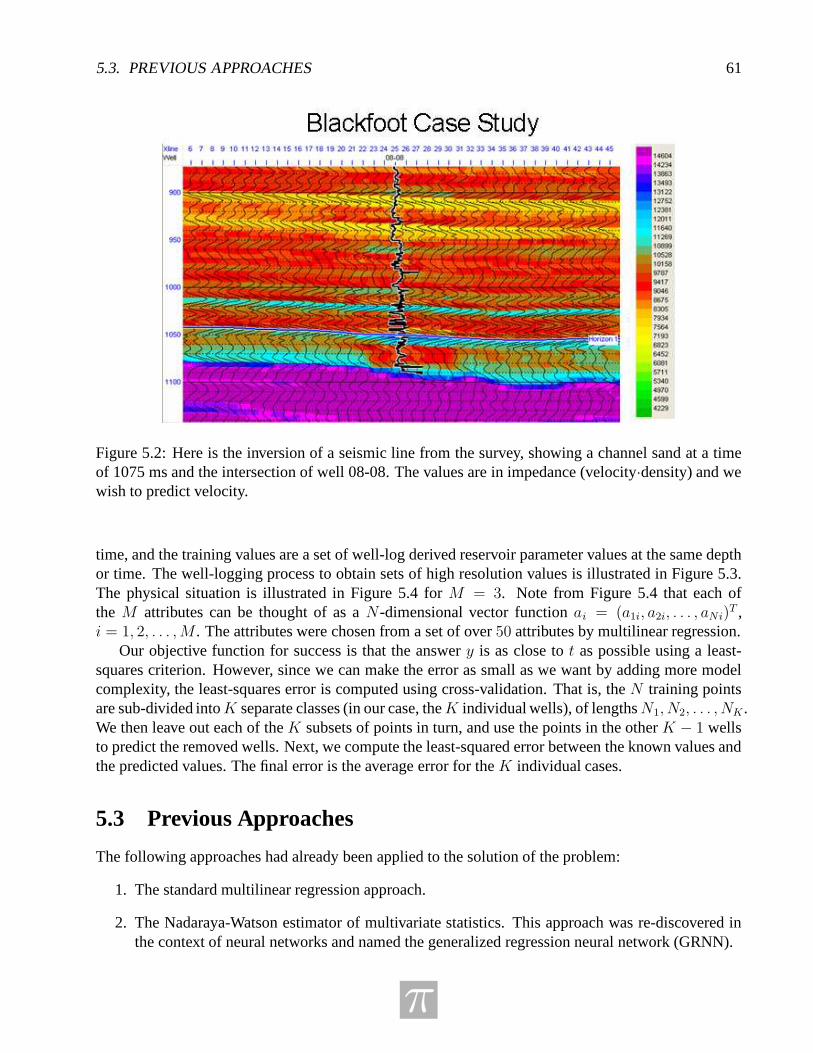
5.3. PREVIOUS APPROACHES 61
Figure 5.2: Here is the inversion of a seismic line from the survey, showing a channel sand at a timeof 1075 ms and the intersection of well 08-08. The values are in impedance (velocity·density) and wewish to predict velocity.
time, and the training values are a set of well-log derived reservoir parameter values at the same depthor time. The well-logging process to obtain sets of high resolution values is illustrated in Figure 5.3.The physical situation is illustrated in Figure 5.4 for M = 3. Note from Figure 5.4 that each ofthe M attributes can be thought of as a N -dimensional vector function ai = (a1i, a2i, . . . , aNi)
T ,i = 1, 2, . . . ,M . The attributes were chosen from a set of over 50 attributes by multilinear regression.
Our objective function for success is that the answer y is as close to t as possible using a least-squares criterion. However, since we can make the error as small as we want by adding more modelcomplexity, the least-squares error is computed using cross-validation. That is, the N training pointsare sub-divided intoK separate classes (in our case, theK individual wells), of lengthsN1, N2, . . . , NK .We then leave out each of the K subsets of points in turn, and use the points in the other K − 1 wellsto predict the removed wells. Next, we compute the least-squared error between the known values andthe predicted values. The final error is the average error for the K individual cases.
5.3 Previous Approaches
The following approaches had already been applied to the solution of the problem:
1. The standard multilinear regression approach.
2. The Nadaraya-Watson estimator of multivariate statistics. This approach was re-discovered inthe context of neural networks and named the generalized regression neural network (GRNN).
π

62 CHAPTER 5. SEISMIC PREDICTION OF RESERVOIR PARAMETERS
Figure 5.3: The well logging procedure directly obtains high resolution values of the desired parame-ters.
3. The radial basis function neural network (RBFN).
The multivariate dataset can be written X = AT , where,
X =[
x1 · · ·xN
]
=
x11 · · · x1N...
. . ....
xM1 · · · xMN ,
, A =
[
a1 · · ·aM
]
=
a11 · · · a1M...
. . ....
aN1 · · · aNM
. (5.2)
5.3.1 Multilinear Regression
Multilinear regression of the attributes against the training values involves solving for the weights inthe equation,
t = w0a0 + w1a1 + · · · + wMaM = Aw, A =
1 a11 · · · a1M...
.... . .
...1 aN1 · · · aNM
, w =
w0...wM
. (5.3)
The solution is found by generalized least-squares to be
w = (AT A+ λI)−1ATt, (5.4)
where λ is a prewhitening factor used to regularize the solution since AT A may not have a stableinverse. Also, too much prewhitening can create artifacts.
π
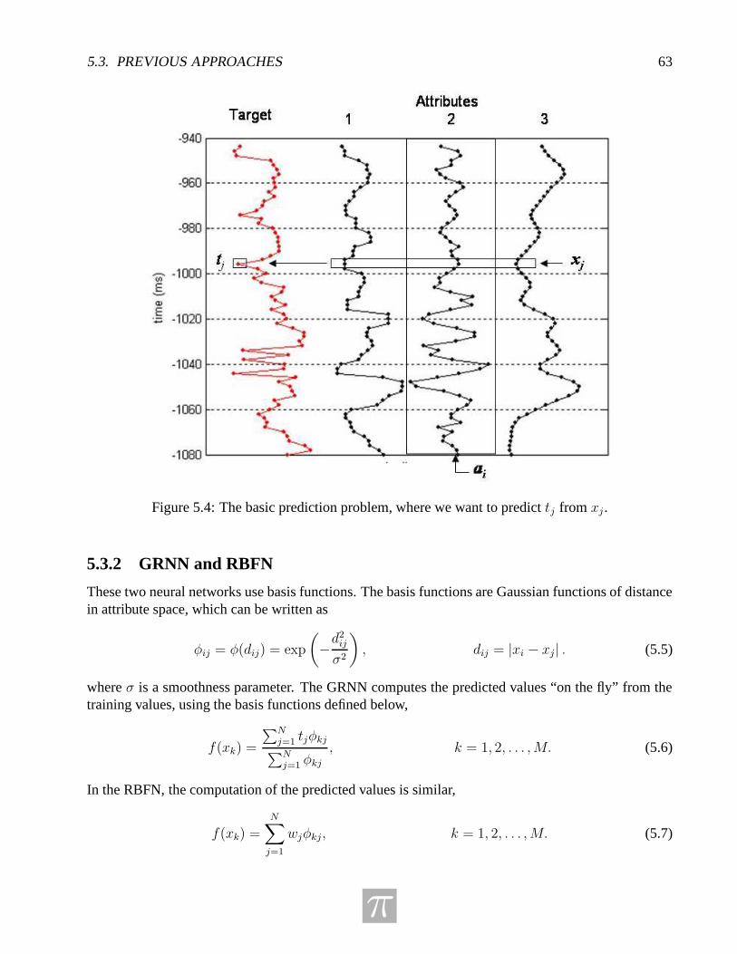
5.3. PREVIOUS APPROACHES 63
Figure 5.4: The basic prediction problem, where we want to predict tj from xj .
5.3.2 GRNN and RBFN
These two neural networks use basis functions. The basis functions are Gaussian functions of distancein attribute space, which can be written as
φij = φ(dij) = exp
(
−d2
ij
σ2
)
, dij = |xi − xj| . (5.5)
where σ is a smoothness parameter. The GRNN computes the predicted values “on the fly” from thetraining values, using the basis functions defined below,
f(xk) =
∑Nj=1 tjφkj
∑Nj=1 φkj
, k = 1, 2, . . . ,M. (5.6)
In the RBFN, the computation of the predicted values is similar,
f(xk) =N
∑
j=1
wjφkj, k = 1, 2, . . . ,M. (5.7)
π

64 CHAPTER 5. SEISMIC PREDICTION OF RESERVOIR PARAMETERS
However, the weights are computed from the training data using the following linear equations,
t(xk) =
N∑
j=1
wjφkj, k = 1, 2, . . . , N. (5.8)
In both GRNN and RBFN, the key parameter to optimize is the σ value, which controls the width ofthe basis functions. For RBFN, we estimate a global value of σ. For GRNN, we optimize σ so that itvaries as a function of the number of parameters in the multivariate observation, or
y(x) =
∑Ni=1 ti exp
[
− (x1−xi1)2
σ2
1
− · · · − (xM−xiM )2
σ2
M
]
∑Ni=1 exp
[
− (x1−xi1)2
σ2
1
− · · · − (xM−xiM )2
σ2
M
] . (5.9)
A comparison of GRNN and RBFN is as follows. The GRNN has a simpler structure and computesits weights directly from the training data without having to pre-compute these weights. The RBFNpre-computes the weights by solving a N ×N matrix, where N is the number of training points. Thetwo methods give similar results for large numbers of training points, but RBFN is superior when thenumber of points is small.
5.3.3 Results
Amongst the three methods, GRNN gives the best results having the highest average correlation coef-ficient between the prediction and the validation target of 12 wells, 0.633. Figure 5.5 shows the bestresult obtained by GRNN, with the correlation coefficient 0.74. It shows the target (red) and predicted(blue) values of velocity versus time of well 11. The worst case has the correlation coefficient 0.47,which is obtained from well 5, and it is shown in Figure 5.6.
5.3.4 Challenges
Thus we have the following challenges:
1. Can we find other methods that may be more accurate?
2. Can we understand the nature and limitations of the methods from our results?
3. Can we devise other more local estimation procedures?
To address these challenges, we have tried the generalized additive model method and the splinemethod. In next two sections, we will describe the two methods and show our results. Finally we willgive the summary of our work in the last section.
5.4 Generalized Additive Model
5.4.1 Introduction of Generalized Additive Model
The Generalized Additive Model (GAM), a generalization of the linear regression model, can beviewed as the combination of the additive model with the generalized linear model. Suppose that
π
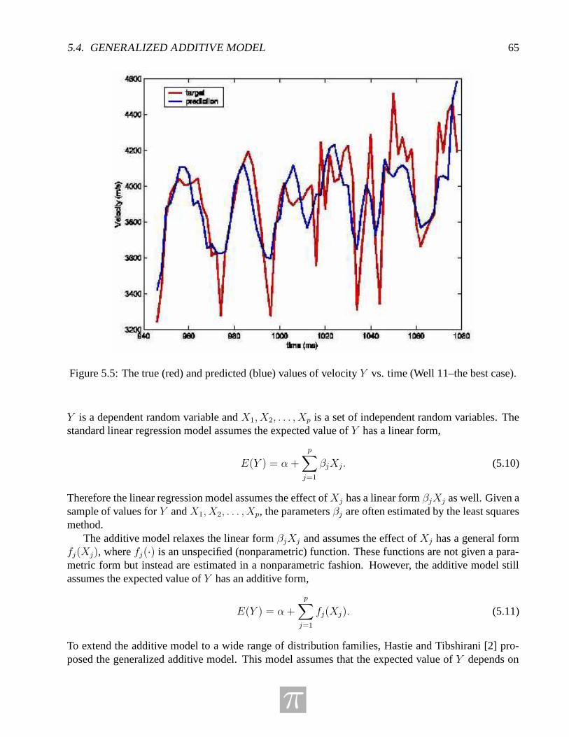
5.4. GENERALIZED ADDITIVE MODEL 65
Figure 5.5: The true (red) and predicted (blue) values of velocity Y vs. time (Well 11–the best case).
Y is a dependent random variable and X1, X2, . . . , Xp is a set of independent random variables. Thestandard linear regression model assumes the expected value of Y has a linear form,
E(Y ) = α +
p∑
j=1
βjXj. (5.10)
Therefore the linear regression model assumes the effect of Xj has a linear form βjXj as well. Given asample of values for Y and X1, X2, . . . , Xp, the parameters βj are often estimated by the least squaresmethod.
The additive model relaxes the linear form βjXj and assumes the effect of Xj has a general formfj(Xj), where fj(·) is an unspecified (nonparametric) function. These functions are not given a para-metric form but instead are estimated in a nonparametric fashion. However, the additive model stillassumes the expected value of Y has an additive form,
E(Y ) = α+
p∑
j=1
fj(Xj). (5.11)
To extend the additive model to a wide range of distribution families, Hastie and Tibshirani [2] pro-posed the generalized additive model. This model assumes that the expected value of Y depends on
π
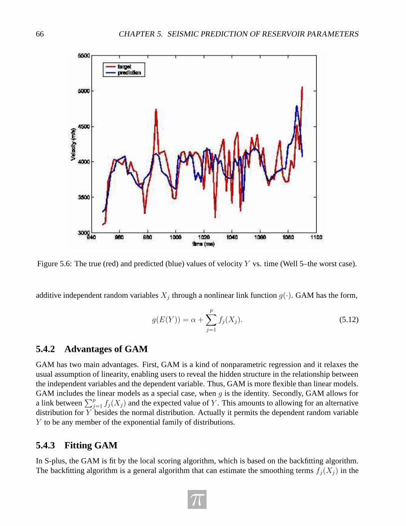
66 CHAPTER 5. SEISMIC PREDICTION OF RESERVOIR PARAMETERS
Figure 5.6: The true (red) and predicted (blue) values of velocity Y vs. time (Well 5–the worst case).
additive independent random variables Xj through a nonlinear link function g(·). GAM has the form,
g(E(Y )) = α+
p∑
j=1
fj(Xj). (5.12)
5.4.2 Advantages of GAM
GAM has two main advantages. First, GAM is a kind of nonparametric regression and it relaxes theusual assumption of linearity, enabling users to reveal the hidden structure in the relationship betweenthe independent variables and the dependent variable. Thus, GAM is more flexible than linear models.GAM includes the linear models as a special case, when g is the identity. Secondly, GAM allows fora link between
∑pj=1 fj(Xj) and the expected value of Y . This amounts to allowing for an alternative
distribution for Y besides the normal distribution. Actually it permits the dependent random variableY to be any member of the exponential family of distributions.
5.4.3 Fitting GAM
In S-plus, the GAM is fit by the local scoring algorithm, which is based on the backfitting algorithm.The backfitting algorithm is a general algorithm that can estimate the smoothing terms fj(Xj) in the
π
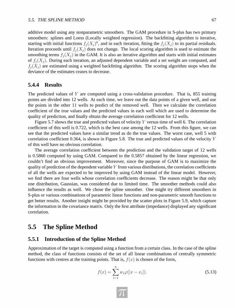
5.5. THE SPLINE METHOD 67
additive model using any nonparametric smoothers. The GAM procedure in S-plus has two primarysmoothers: splines and Loess (Locally weighted regression). The backfitting algorithm is iterative,starting with initial functions fj(Xj)
0, and in each iteration, fitting the fj(Xj) to its partial residuals.Iteration proceeds until fj(Xj) does not change. The local scoring algorithm is used to estimate thesmoothing terms fj(Xj) in the GAM. It is also an iterative algorithm and starts with initial estimatesof fj(Xj). During each iteration, an adjusted dependent variable and a set weight are computed, andfj(Xj) are estimated using a weighted backfitting algorithm. The scoring algorithm stops when thedeviance of the estimates ceases to decrease.
5.4.4 Results
The predicted values of Y are computed using a cross-validation procedure. That is, 855 trainingpoints are divided into 12 wells. At each time, we leave out the data points of a given well, and usethe points in the other 11 wells to predict of the removed well. Then we calculate the correlationcoefficient of the true values and the predicted values in each well which are used to determine thequality of prediction, and finally obtain the average correlation coefficient for 12 wells.
Figure 5.7 shows the true and predicted values of velocity Y versus time of well 6. The correlationcoefficient of this well is 0.722, which is the best case among the 12 wells. From this figure, we cansee that the predicted values have a similar trend as do the true values. The worst case, well 5 withcorrelation coefficient 0.364, is shown in Figure 5.8. The true and predicted values of the velocity Yof this well have no obvious correlation.
The average correlation coefficient between the prediction and the validation target of 12 wellsis 0.5860 computed by using GAM. Compared to the 0.5857 obtained by the linear regression, wecouldn’t find an obvious improvement. Moreover, since the purpose of GAM is to maximize thequality of prediction of the dependent variable Y from various distributions, the correlation coefficientsof all the wells are expected to be improved by using GAM instead of the linear model. However,we find there are four wells whose correlation coefficients decrease. The reason might be that onlyone distribution, Gaussian, was considered due to limited time. The smoother methods could alsoinfluence the results as well. We chose the spline smoother. One might try different smoothers inS-plus or various combinations of parametric linear functions and non-parametric smooth functions toget better results. Another insight might be provided by the scatter plots in Figure 5.9, which capturethe information in the covariance matrix. Only the first attribute (impedance) displayed any significantcorrelation.
5.5 The Spline Method
5.5.1 Introduction of the Spline Method
Approximation of the target is computed using a function from a certain class. In the case of the splinemethod, the class of functions consists of the set of all linear combinations of centrally symmetricfunctions with centres at the training points. That is, f(x) is chosen of the form,
f(x) =n
∑
i=1
wiϕ(|x− xi|). (5.13)
π
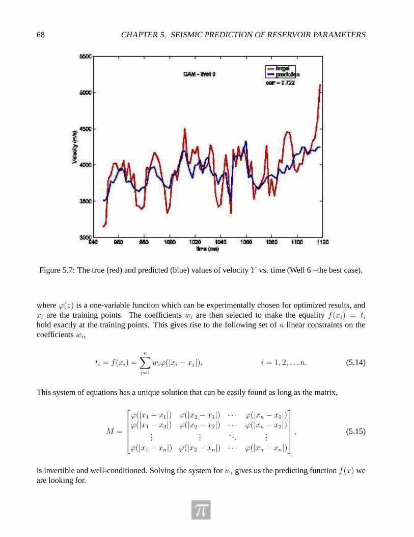
68 CHAPTER 5. SEISMIC PREDICTION OF RESERVOIR PARAMETERS
Figure 5.7: The true (red) and predicted (blue) values of velocity Y vs. time (Well 6 –the best case).
where ϕ(z) is a one-variable function which can be experimentally chosen for optimized results, andxi are the training points. The coefficients wi are then selected to make the equality f(xi) = tihold exactly at the training points. This gives rise to the following set of n linear constraints on thecoefficients wi,
ti = f(xi) =n
∑
j=1
wiϕ(|xi − xj|), i = 1, 2, . . . n. (5.14)
This system of equations has a unique solution that can be easily found as long as the matrix,
M =
ϕ(|x1 − x1|) ϕ(|x2 − x1|) · · · ϕ(|xn − x1|)ϕ(|x1 − x2|) ϕ(|x2 − x2|) · · · ϕ(|xn − x2|)
......
. . ....
ϕ(|x1 − xn|) ϕ(|x2 − xn|) · · · ϕ(|xn − xn|)
, (5.15)
is invertible and well-conditioned. Solving the system for wi gives us the predicting function f(x) weare looking for.
π
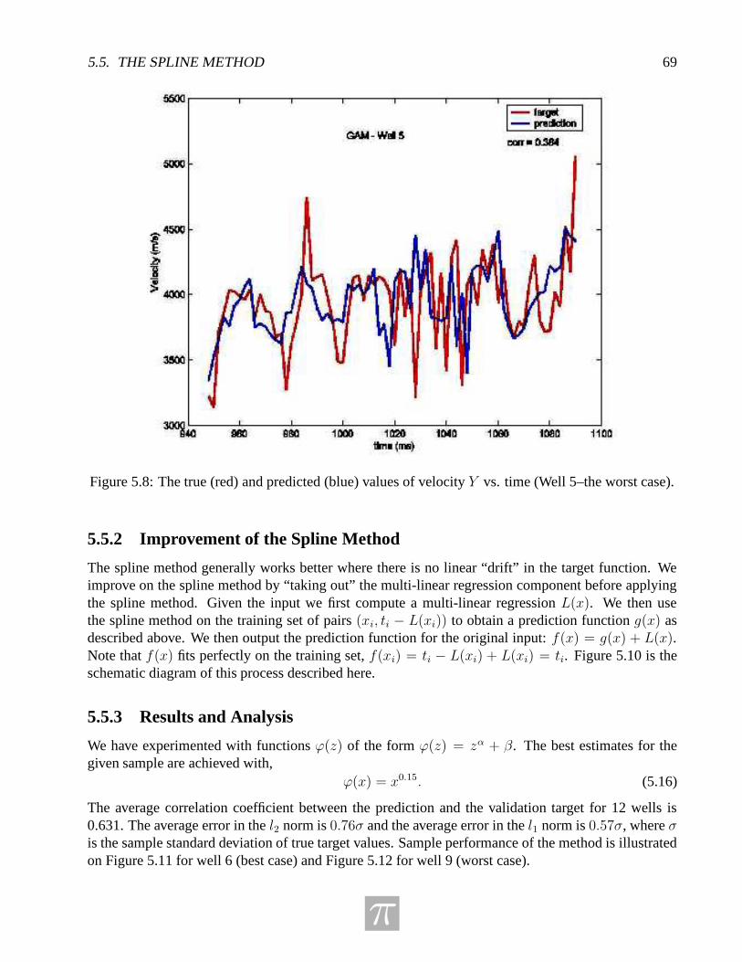
5.5. THE SPLINE METHOD 69
Figure 5.8: The true (red) and predicted (blue) values of velocity Y vs. time (Well 5–the worst case).
5.5.2 Improvement of the Spline Method
The spline method generally works better where there is no linear “drift” in the target function. Weimprove on the spline method by “taking out” the multi-linear regression component before applyingthe spline method. Given the input we first compute a multi-linear regression L(x). We then usethe spline method on the training set of pairs (xi, ti − L(xi)) to obtain a prediction function g(x) asdescribed above. We then output the prediction function for the original input: f(x) = g(x) + L(x).Note that f(x) fits perfectly on the training set, f(xi) = ti − L(xi) + L(xi) = ti. Figure 5.10 is theschematic diagram of this process described here.
5.5.3 Results and Analysis
We have experimented with functions ϕ(z) of the form ϕ(z) = zα + β. The best estimates for thegiven sample are achieved with,
ϕ(x) = x0.15. (5.16)
The average correlation coefficient between the prediction and the validation target for 12 wells is0.631. The average error in the l2 norm is 0.76σ and the average error in the l1 norm is 0.57σ, where σis the sample standard deviation of true target values. Sample performance of the method is illustratedon Figure 5.11 for well 6 (best case) and Figure 5.12 for well 9 (worst case).
π
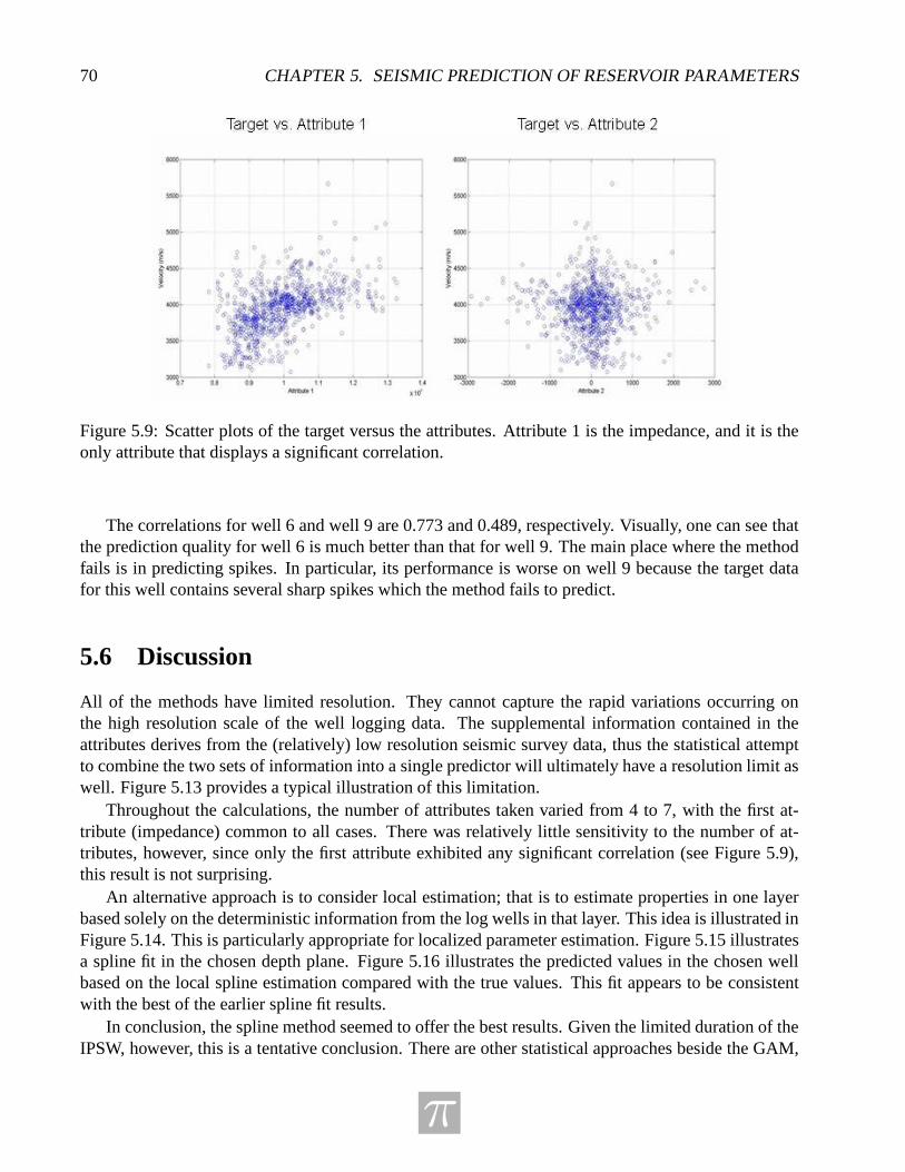
70 CHAPTER 5. SEISMIC PREDICTION OF RESERVOIR PARAMETERS
Figure 5.9: Scatter plots of the target versus the attributes. Attribute 1 is the impedance, and it is theonly attribute that displays a significant correlation.
The correlations for well 6 and well 9 are 0.773 and 0.489, respectively. Visually, one can see thatthe prediction quality for well 6 is much better than that for well 9. The main place where the methodfails is in predicting spikes. In particular, its performance is worse on well 9 because the target datafor this well contains several sharp spikes which the method fails to predict.
5.6 Discussion
All of the methods have limited resolution. They cannot capture the rapid variations occurring onthe high resolution scale of the well logging data. The supplemental information contained in theattributes derives from the (relatively) low resolution seismic survey data, thus the statistical attemptto combine the two sets of information into a single predictor will ultimately have a resolution limit aswell. Figure 5.13 provides a typical illustration of this limitation.
Throughout the calculations, the number of attributes taken varied from 4 to 7, with the first at-tribute (impedance) common to all cases. There was relatively little sensitivity to the number of at-tributes, however, since only the first attribute exhibited any significant correlation (see Figure 5.9),this result is not surprising.
An alternative approach is to consider local estimation; that is to estimate properties in one layerbased solely on the deterministic information from the log wells in that layer. This idea is illustrated inFigure 5.14. This is particularly appropriate for localized parameter estimation. Figure 5.15 illustratesa spline fit in the chosen depth plane. Figure 5.16 illustrates the predicted values in the chosen wellbased on the local spline estimation compared with the true values. This fit appears to be consistentwith the best of the earlier spline fit results.
In conclusion, the spline method seemed to offer the best results. Given the limited duration of theIPSW, however, this is a tentative conclusion. There are other statistical approaches beside the GAM,
π
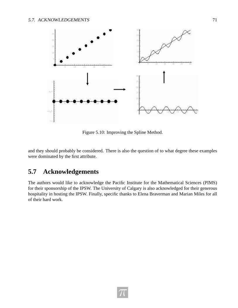
5.7. ACKNOWLEDGEMENTS 71
Figure 5.10: Improving the Spline Method.
and they should probably be considered. There is also the question of to what degree these exampleswere dominated by the first attribute.
5.7 Acknowledgements
The authors would like to acknowledge the Pacific Institute for the Mathematical Sciences (PIMS)for their sponsorship of the IPSW. The University of Calgary is also acknowledged for their generoushospitality in hosting the IPSW. Finally, specific thanks to Elena Braverman and Marian Miles for allof their hard work.
π
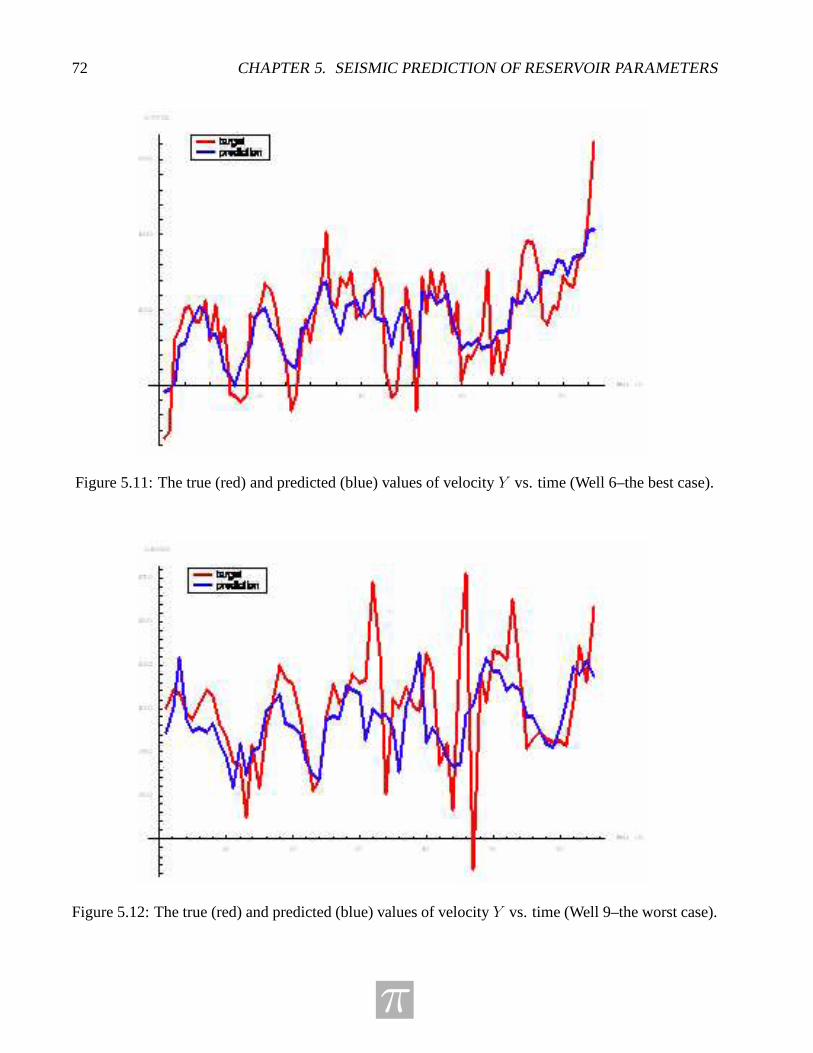
72 CHAPTER 5. SEISMIC PREDICTION OF RESERVOIR PARAMETERS
Figure 5.11: The true (red) and predicted (blue) values of velocity Y vs. time (Well 6–the best case).
Figure 5.12: The true (red) and predicted (blue) values of velocity Y vs. time (Well 9–the worst case).
π
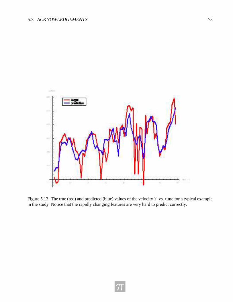
5.7. ACKNOWLEDGEMENTS 73
Figure 5.13: The true (red) and predicted (blue) values of the velocity Y vs. time for a typical examplein the study. Notice that the rapidly changing features are very hard to predict correctly.
π
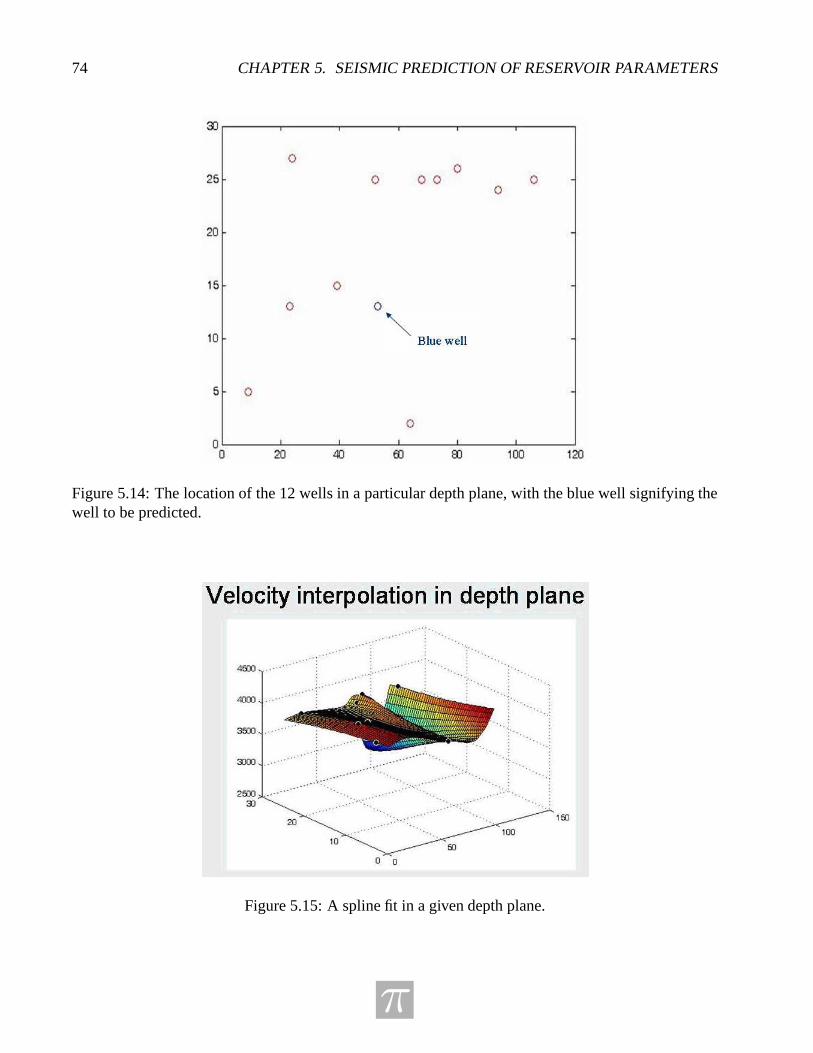
74 CHAPTER 5. SEISMIC PREDICTION OF RESERVOIR PARAMETERS
Figure 5.14: The location of the 12 wells in a particular depth plane, with the blue well signifying thewell to be predicted.
Figure 5.15: A spline fit in a given depth plane.
π
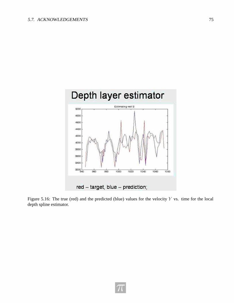
5.7. ACKNOWLEDGEMENTS 75
Figure 5.16: The true (red) and the predicted (blue) values for the velocity Y vs. time for the localdepth spline estimator.
π

76 CHAPTER 5. SEISMIC PREDICTION OF RESERVOIR PARAMETERS
π

Bibliography
[1] Bishop, C. M. (1995). Neural Networks for Patten Recognition. Oxford University Press.
[2] Hastie, T. & Tibshirani, R. (1990). Generalized additive models. Chapman & Hall: New York.
[3] Johnson, R. A. & Wichern, D. W. (1998). Applied Multivariate Statistical Analysis. Prentice Hall.
[4] Masters, T. (1995). Advanced Algorithms for Neural Networks. John Wiley & Sons, Inc.
[5] Russell, B. (2005). The Application of Multivariate Statistics and Neural Networks to the Predic-tion of Reservoir Parameters from Seismic Attributes: Ph.D. dissertation, University of Calgary.
[6] Russell, B. (2005). Seismic Prediction of Reservoir Parameters (An IPSW Problem).
77

78 BIBLIOGRAPHY
π

Appendix A
List of Participants
Mahmud Akelbek University of Regina [email protected] Amiraslani University of Western Ontario [email protected] Artoun Concordia University eugenie [email protected] Bondy Genus Capital Management [email protected] Bos University of Calgary [email protected] Braverman University of Calgary [email protected] Braverman University of Toronto [email protected] Chen University of Calgary [email protected] Clysdale University of Calgary [email protected] David-Rus Rutgers University [email protected] Emmett University of Calgary [email protected] Fishman MDF International, University of Calgary [email protected] Fital University of Regina [email protected] Gonzalez Northeastern University [email protected] Griffin Washington State University [email protected] Henderson University of Calgary [email protected] Hogan University of Calgary [email protected] Holloway University of Alberta [email protected] Huang University of British Columbia [email protected] Hughes University of Calgary [email protected] Jamali University of Western Ontario [email protected] K. Cole Biomechanigg Research Inc. [email protected] Lamoureux University of Calgary [email protected] Lemire Calgary Scientific Inc. [email protected] Lewis University of Ontario [email protected] Li University of Calgary [email protected] Lim University of Colorado [email protected] Lushi Simon Fraser University [email protected] Ma University of Calgary [email protected] Mackenzie University of CalgaryMaryam Mizani University of Victoria [email protected]
79

80 APPENDIX A. LIST OF PARTICIPANTS
Mahyar Mohajer University of Calgary [email protected] Monthubert Institut de Mathematiques de Toulouse [email protected] Nouri University of Western Ontario [email protected] Odegaard University of Western Ontario [email protected] Orosi University of Calgary [email protected] Ping Liu University of Regina [email protected] Pinnegar Calgary Scientific Inc.Hatesh Radia University of Massachusetts at Lowell [email protected] Ren University of British Columbia [email protected] Rezvani University of Western Ontario [email protected] Russell Hampson Russell Software brian [email protected]. Sean Bohun Pennsylvania State University [email protected] Smith Memorial University of Newfoundland [email protected] Sun University of Calgary [email protected] Thomas University of Lethbridge [email protected] Vaidya York University [email protected] Wang Simon Fraser University [email protected] Ware University of Calgary [email protected] Westbrook University of Calgary [email protected] Williams University of California, Davis [email protected] Xu University of Washington [email protected] Xu York University [email protected] Yin University of Saskatchewan [email protected] Zhang University of Saskatchewan [email protected]
π


PIMS Contact Information
email: [email protected]
http://www.pims.math.ca
Pacific Institute for the Mathematical SciencesCentral Office
Room 200, 1933 West MallUniversity of British Columbia
Vancouver BC V6T 1Z2Canada