arX

iv:1

501.

0251

3v2

[m

ath.

PR]

20

Aug

201

5

The 20-60-20 Rule

Piotr Jaworski∗, Marcin Pitera†,

August 21, 2015

Abstract

In this paper we discuss an empirical phenomena known as the 20-60-20 rule. It says that if wesplit the population into three groups, according to some arbitrary benchmark criterion, then thisparticular ratio implies some sort of balance. From practical point of view, this feature often leads toefficient management or control. We provide a mathematical illustration, justifying the occurrence ofthis rule in many real world situations. We show that for any population, which could be describedusing multivariate normal vector, this fixed ratio leads to a global equilibrium state, when dispersionand linear dependance measurement is considered.

Keywords: 20-60-20 Rule, 60/20/20 Principle, 20:60:20, Pareto principle, law of the vital few, theprinciple of factor sparsity, truncated normal distribution, conditional elliptic distribution.

MSC2010: 60K30, 91B10, 91B14, 91B52. 60A86, 62A86,

Introduction

The 20-60-20 rule is an empirical statement. It says that if we want to split the population into threegroups, using some arbitrary benchmark criterion, then the ratio of 20%, 60% and 20% proves to givean efficient partition. The division is usually made according to the performance of each element in thepopulation and the groups are referred to as negative, neutral and positive, respectively. The first grouprelates to elements of population which positively contribute to the considered subject (e.g. effectiveworkers, top sale managers, productive members), while the last one denotes the opposite. The middleset corresponds to the middle part of the population, having average performance. Putting it anotherway we cluster the population basing on a notion of effectiveness.

The importance of this rule comes from the fact that this particular partition seems to be the mosteffective one, for many empirical problems. Let us present in details two common illustrations of thisphenomena and then comment on the efficiency to make this idea more transparent.

The first example considers sales departments. In almost any big company, the employees of thesales department could be split into three groups, maintaining 20-60-20 ratio. The first group are topperformers, who make big profits, even without supervision. The middle group are people who need tobe managed to make average but stable profits. The last group are people who are heading towardstermination or resignation. They produce no good income, even when supervised.

The second example relates to change capability. If you are willing to make substantial changes inany big institution, then on average 20% of the people are ready, willing and able to change, while 20%of people would not accept the change, whatever the cost. The middle 60% will wait to see how thesituation turns out.

Corporations use the 20-60-20 rule widely in management and sales departments [15, 13]. One of thepractical aspects of this phenomena relates to the fact that different procedures and methods are createdto handle the efficiency in positive, negative and neutral group and the 20-60-20 ratio proves to be themost efficient partition. For example, in many problems related to human resource management, oneshould identify and focus his attention on the middle 60%, as this group could and should be managedefficiently.

∗Institute of Mathematics, University of Warsaw, Warsaw, Poland.†Institute of Mathematics, Jagiellonian University, Cracow, Poland.

1

Of course there are countless illustrations of this phenomena. One could consider financial marketoverall condition, fraud and theft capability among group of people, the structure of electorate, sportperformance among athletes, potential of students, patient handling, medical treatments, etc. Please seee.g. [14, 3, 1, 5, 7, 8, 11, 2, 4], where the 20-60-20 ratio is used and the detailed procedures are proposedto handle many practical problems.

The natural question is why this specific 20/60/20 ratio is valid in so many situations? Why not10/80/10 or 30/40/30? Is this a coincidence, or does it follow from some underlying and fundamentalstructure of the population?

While very popular among practitioners, no scientific evidence of the 20-60-20 principle has beenpresented yet, due to the authors knowledge. Consequently, this noteworthy rule become more of aslogan, than the scientific fact.

The possible mathematical illustration of this phenomena, based on the dispersion and linear depen-dance measurement will be the main topic of this paper. We will show that if a (multivariate) randomvector is distributed normally and we do conditioning based on the (quantile function of) first coordinate,then the ratio close to 20/60/20 imply a global equilibrium state, when dispersion and linear dependancemeasurement is considered. In particular, we prove that this particular partition implies the equalityof covariance matrices, for all conditional vectors, implying some sort of global balance in the popula-tion. We will also discuss the case of monotone dependance using conditional Kendall τ and Spearmanρ matrices.

The material is organized as follows. The introduction is followed by a short preliminaries, where weestablish basic notations used throughout this paper. Next, in Section 2 we introduce a mathematicalmodel for the 20-60-20 rule and define the equilibrium state, using conditional covariance matrices. The20-60-20 rule for multivariate normal vectors is discussed in Section 3. Theorem 1 might be considered asthe main result of this paper. Section 4 is devoted to the study of different equilibrium states, obtainedusing correlation matrices, Kendall τ matrices and Spearman ρ matrices. In particular we present heresome theoretical results, when Spearman ρ matrices are considered and a numerical example, illustratingthe 20-60-20 rule for sample data. In Section 5 we discuss shortly what happens if we loose the assumptionabout normality. The general elliptic case is considered here.

1 Preliminaries

Let (Ω,Σ,P) be a probability space and let n ∈ N. Let us fix an n-dimensional continuous random vectorX = (X1, . . . , Xn). We will use

H(x1, . . . , xn) := P[X1 ≤ x1, . . . Xn ≤ xn],

to denote the corresponding joint distribution function and

Hi(x) = P[Xi ≤ x], i = 1, 2, . . . , n,

to denote the marginal distribution functions. Given a Borel set B in Rn such that

P[ω ∈ Ω : (X1(ω), . . . , Xn(ω)) ∈ B] > 0

we can define the conditional distribution HB for all (x1, . . . , xn) ∈ B by

HB(x1, . . . , xn) = P[X1 ≤ x1, . . . , Xn ≤ xn | X ∈ B]. (1)

Putting it in another words we truncate the random vector X to the Borel set B. If necessary, we assumethe existence of regular conditional probabilities. In this paper we will assume that B is a non-degeneraterectangle, i.e. B ∈ R, where

R := A ∈ Rn : A = [a1, b1]× [a2, b2]× . . .× [an, bn], where an, bn ∈ R and an < bn.

As we will be mainly interested in quantile-based conditioning on the first coordinate, for q1, q2 ∈ [0, 1]such that q1 < q2, we shall use notation

H[q1,q2](x1, . . . , xn) := HB(q1,q2)(x1, . . . , xn), (2)

2

where the conditioning set is given by

B(q1, q2) := [H−11 (q1), H

−11 (q2)]× R× . . .× R.

We shall also refer to H[q1,q2] as the truncated distribution, while B(q1, q2) will be called truncation interval(see [10]).

Moreover, we will denote by µ = (µ1, . . . , µn) and Σ = σ2iji,j=1,...,n, the mean vector and covariance

matrix of X . Similarly as in formula (1), given B, we will use µB and ΣB to denote the conditional meanvector and the conditional covariance matrix, i.e. mean vector and conditional covariance matrix of arandom vector with distribution HB. Consequently, as in (2), we shall write

µ[q1,q2] := µB(q1,q2) and Σ[q1,q2] := ΣB(q1,q2).

We will also use Φ and φ to denote the distribution and density function of a standard univariate normaldistribution, respectively.

2 The global balance

To split the whole population into three separate groups basing on a notion of effectiveness, we need tomake an assumption about the probability distribution of the whole population and the given benchmark,which measures the effectiveness of each element in the population. We will assume that X ∼ N (µ,Σ),i.e. the population could be described using n-dimensional random vector X = (X1, . . . , Xn), which isnormally distributed with mean vector µ and covariance matrix Σ. Furthermore, we will assume thatthe benchmark level is determined by the first coordinate, i.e. X1. Please note that for multivariatenormal this may be a linear combination of all other coordinates. One could look at other coordinates asvarious factors, which could influence the main benchmark. Note that, if we talk about people measuresor abilities, then Gaussian functions, often described as bell curves, are a natural choice.

We will seek for two real numbers q1, q2 ∈ [0, 1] and the corresponding partition

B(0, q1), B(q1, 1− q2), B(1− q2, 1),

which will admit some sort of equilibrium. In other words, we want to divide the whole population intothree subgroups, corresponding to the lower 100q1%, the middle 100(1− q1− q2)% and the upper 100q2%of the population, where the effectiveness is measured by the benchmark. To do so, let us give a definitionof equilibrium state or global balance.

Definition 1. We will say that a global balance (or equilibrium state) is achieved in X if

Σ[0,q1] = Σ[q1,1−q2] = Σ[1−q2,1], (3)

for some q1, q2 ∈ [0, 1], such that q1 < q2.

Definition 1 seems to be very intuitive. Indeed, the equality of conditional covariance matrices saythat:

1. The dispersion measured by variance is the same in each subgroup for any coordinate Xi (fori = 1, 2, . . . , n). In particular the dispersion of the benchmark is the same everywhere.

2. The linear dependance structure, measured by the conditional correlation matrices, is the same inall three subgroups.

The first property creates a natural equilibrium state, as any perturbation leads to irregularity, whenthe square distance from the average member of each group is considered. The choice of this measure ofdispersion seems to be natural, because people awareness of any differences should be high, as variance(or standard deviation) seems to be the simplest measure of variability.

The second property relate to the linear dependence structure. The equality of correlation matricesimply a natural equilibrium between groups, as people tend to notice the simplest (linear) dependanciesfirst. Any shift between groups will cause dependence instability between them.

In general (i.e. when we loose assumption about normality) the global balance might not exists orstrongly depend on initial Σ, when we consider some family parametrised by covariance matrices.

3

3 The 20/60/20 principle

If X is a multivariate normal, it is reasonable to set q1 = q2, due to the symmetry of the Gaussiandensity. For simplicity we will use q = q1 = q2 for the symmetric case. Thus, we will in fact seek forq ∈ (0, 0.5) such that the conditional covariance matrix for the lower 100q% of the population coincidewith the conditional covariance matrices of the middle 100(1− 2q)% and upper 100q%.

We are now ready to present the main result of this paper. We will show that if X ∼ N (µ,Σ), thenthe equilibrium state will be achieved for the unique q ∈ (0, 0.5). This is a statement of Theorem 1.

Theorem 1. Let X ∼ N (µ,Σ). Then there exists a unique q ∈ (0, 0.5) such that the global balance inX is achieved, i.e. the equality (3) is true for q = q1 = q2. Moreover, the value of q is independent of µand Σ and the approximate value of q is 0,198089616...

The proof of Theorem 1 is surprisingly simple. It is a direct consequence of Lemma 1 and Lemma 2,which we will now present and prove. Before we do this, let us give a comment on Theorem 1. It says thatif we split the whole population, into three separate groups, then the ratio close to 20-60-20 (and in factonly this ratio), will imply the equality of conditional covariance matrices for all groups, creating a naturalequilibrium. To prove Theorem 1 we need an analytic formula for conditional covariance structure, givenany conditioning Borel set B of positive measure. This will be the statement of Lemma 1.

Lemma 1. Let X ∼ N (µ,Σ). Then for any Borel subset B of R with positive measure,

ΣB = Σ+ (D2[X1 | X1 ∈ B]−D2[X1])ββT ,

where

βT = (β1, . . . , βn), βi =Cov[X1, Xi]

D2[X1].

Proof of Lemma 1. Being in Gaussian world we can describe each random variable Xi as a combinationof the random variable X1 and a random variable Yi independent of X1. Indeed, we put for i = 1, . . . , n

Yi = Xi − βiX1, where βi =Cov[X1, Xi]

D2[X1]. (4)

Obviously β1 = 1 and Y1 = 0. Since for i = 2, . . . , n, the newly defined variable Yi is uncorrelated withX1, they are independent.Next, we calculate the conditional covariance matrix. Using (4), we get for i, j = 1, . . . , n

Cov[Xi, Xj | X1 ∈ B] = Cov[βiX1 + Yi, βjX1 + Yj | X1 ∈ B].

Since Yi and Yj do not dependent on X1, we get

Cov[Yi, X1 | X1 ∈ B] = 0 = Cov[Yj , X1 | X1 ∈ B],

andCov[Yi, Yj | X1 ∈ B] = Cov[Yi, Yj ] = Cov[Xi, Xj ]− βiβjD

2[X1].

Therefore, we obtain

Cov[Xi, Xj | X1 ∈ B] = Cov[Xi, Xj] + βiβj(D2[X1 | X1 ∈ B]−D2[X1]).

Since βiβj is the i, j-th entry of the n× n matrix ββT , we finish the proof of the lemma.

From Lemma 1 we see, that we can parametrise ΣB in such a way, that it will only depend on theconditional variance of X1. Thus, we only need to show that there exists q ∈ (0, 0.5) such that the(conditional) dispersion of X1 in all three groups, determined by sets B(0, q), B(q, 1− q) and B(1− q, 1)will coincide. This will be the statement of Lemma 2.

4

Lemma 2. Let X1 ∼ N (µ1, σ211). Then there exist a unique q ∈ (0, 0.5) such that

D2[X1 | X1 ∈ B(0, q)] = D2[X1 | X1 ∈ B(q, 1− q)] = D2[X1 | X1 ∈ B(1− q, 1)].

Moreover, q = Φ(x), where x < 0 is the unique negative solution of the following equation

− xΦ(x) = φ(x)(1 − 2Φ(x)), (5)

where φ and Φ denote the density and distribution function of standard normal, respectively. The ap-proximate value of q is 19,8089616....

Proof of Lemma 2. Without any loss of generality we may assume that X1 has the standard normaldistribution N (0, 1). Indeed, for Xst

1 = X1−µ1

σ11

, and q1, q2 ∈ [0, 1], such that q1 < q2, we get

D2[

X1 | H1(X1) ∈ [q1, q2]]

= D2[

σ11Xst1 + µ1 | Φ(Xst

1 ) ∈ [q1, q2]]

= σ211D

2[

Xst1 | Φ(Xst

1 ) ∈ [q1, q2]]

.

To proceed, we need to compute the first two moments of the truncated normal distribution of X1.For transparency, we will show full proofs (compare [10, Section 13.10.1]).

Let us calculate the conditional expectations E[X1 | X1 < x] and E[X1 | x < X1 < −x] for any fixedx ∈ (−∞, 0). Since φ′(x) = −xφ(x), we get

E[X1 | X1 < x] =1

Φ(x)

∫ x

−∞

ξφ(ξ)dξ =1

Φ(x)(−φ(ξ))|x−∞ = −φ(x)

Φ(x),

E[X1 | x < X1 < −x] = 0.

To get the corresponding second moments we integrate by parts.

E[X21 | X1 < x] =

1

Φ(x)

∫ x

−∞

ξ2φ(ξ)dξ =1

Φ(x)

(

−ξφ(ξ))|x−∞ +

∫ x

−∞

φ(ξ)dξ

)

=1

Φ(x)(−xφ(x) + Φ(x)) = 1− xφ(x)

Φ(x),

E[X21 | x < X1 < −x] =

1

1− 2Φ(x)

∫ −x

x

ξ2φ(ξ)dξ =1

1− 2Φ(x)

(

−ξφ(ξ))|−xx +

∫ −x

x

φ(ξ)dξ

)

=1

1− 2Φ(x)(2xφ(x) + 1− 2Φ(x)) = 1 +

2xφ(x)

1− 2Φ(x).

Therefore,

D2[X1 | X1 < x] = 1− xφ(x)

Φ(x)− φ(x)2

Φ(x)2,

D2[X1 | x < X1 < −x] = 1 +2xφ(x)

1− 2Φ(x).

Since the conditional expected value behaves like a weighted arithmetic mean, we get that E[X1 | X1 < x]is strictly increasing in x, while E[X2

1 | x < X1 < −x] and E[X21 | X1 < x] are strictly decreasing with

respect to x. Consequently, the central conditional variance D2[X1 | x < X1 < −x] is strictly decreasing.Next, we will show that the tail conditional variance D2[X1 | X1 < x] is strictly increasing. Indeed,

d

dxD2[X1 | X1 < x] = − φ(x)

Φ(x)+ x2 φ(x)

Φ(x)− x

φ(x)2

Φ(x)+ 2x

φ(x)2

Φ(x)+ 2

φ(x)2

Φ(x)2

=φ(x)

Φ(x)

(

x2 − 1 + xφ(x)

Φ(x)+ 2

φ(x)2

Φ(x)2

)

=φ(x)

Φ(x)

(

(

x2 − 1

2

φ(x)

Φ(x)

)2

+7

4

φ(x)2

Φ(x)2− 1

)

> 0.

The last inequality follows from the fact that since φ(x)Φ(x) = −E[X1 | X1 < x] is decreasing and positive,

we getφ(x)2

Φ(x)2≥ φ(0)2

Φ(0)2=

2

π>

4

7.

5

Next, note that (compare [9, Lemma 8.1])

limx→−∞

D2[X1 | X1 < x] = 0 and D2[X1 | X1 < 0] = 1− 2

π,

whilelim

x→−∞D2[X1 | x < X1 < −x] = 1 and lim

x→0D2[X1 | x < X1 < −x] = 0.

Hence there exists a unique x < 0 such that

D2[X1 | X1 < x] = D2[X1 | x < X1 < −x].

Compare Figure 1 for visualization.

0.0 0.1 0.2 0.3 0.4 0.5

0.0

0.2

0.4

0.6

0.8

1.0

q

varia

nce

B[0,q] (tail)B[q,1−q] (central)

Figure 1: The graph of conditional tail variance D2[X1 | X1 ∈ B(0, q)] and conditional central varianceD2[X1 | X1 ∈ B(q, 1− q)] as functions of q ∈ (0, 0.5), under the assumption X1 ∼ N (0, 1).

Moreover,

D2[X1 | X1 < x]−D2[X1 | x < X1 < −x] = 1− xφ(x)

Φ(x)− φ(x)2

Φ(x)2− 1− 2xφ(x)

1− 2Φ(x)

=Φ(x)

Φ(x)2(1− 2Φ(x))(−xΦ(x)− φ(x)(1 − 2Φ(x))) ,

which shows that x is a (negative) solution of equation (5). Using basic numerical tools we checkedthat (5) is satisfied for x ≈ −0, 8484646848, for which Φ(x) ≈ 0, 198089615.

Theorem 1 provides an illustration to the empirical 20-60-20 rule. In particular we have shown that forany multivariate normal vector, this fixed ratio leads to a global equilibrium state, when dispersion andlinear dependance measurement is considered. Nevertheless, please note, that the equality of conditionalvariances does not imply the equality of conditional distributions, as could be seen in Figure 1.

Also, while linear dependance structure will be the same, the overall dependance in each subgroup,measured e.g. by the copula function [12], will be different. Indeed, for example it seems to be unwiseto require the dependance structure in the best group, to coincide with the dependance structure in theaverage group. See Figure 2 for an illustrative example.

Remark 1. The equilibrium level q calculated in Lemma 2 depends neither on µ nor Σ. Therefore, ifwe consider correlation matrices instead of covariance matrices in (3), then the optimal value of q fromTheorem 1 will also imply the corresponding equilibrium state, for correlation matrices.1

1Please note we need additional assumption that X1 is not independent of (X2, . . . ,Xn) as otherwise any q ∈ (0, 0.5)will satisfy (3) for correlation matrices instead of covariance matrices.

6

−3 −2 −1 0 1 2 3

0.0

0.2

0.4

0.6

0.8

1.0

1.2

1.4

−3 −2 −1 0 1 2 3

0.0

0.2

0.4

0.6

0.8

1.0

1.2

1.4

−3 −2 −1 0 1 2 3

0.0

0.2

0.4

0.6

0.8

1.0

1.2

1.4

Figure 2: The conditional density function of the lower 20%, middle 60% and upper 20% of the standardnormal distribution. The conditional variances for all three cases coincide.

−3 −2 −1 0 1 2 3

−3

−2

−1

01

23

−3 −2 −1 0 1 2 3

−3

−2

−1

01

23

−3 −2 −1 0 1 2 3

−3

−2

−1

01

23

0.0 0.2 0.4 0.6 0.8 1.0

0.0

0.2

0.4

0.6

0.8

1.0

0.0 0.2 0.4 0.6 0.8 1.0

0.0

0.2

0.4

0.6

0.8

1.0

0.0 0.2 0.4 0.6 0.8 1.0

0.0

0.2

0.4

0.6

0.8

1.0

Figure 3: The conditional samples (upper row) and their conditional copula functions (lower row) fromthe bivariate normal with µ = (0, 0) and Σ = σij , where σ11 = σ22 = 1 and σ12 = σ21 = 0.8. Theconditioning is based on the the first coordinate and relates to the lower 20%, middle 60% and upper20% of the whole population.

Remark 2. The value ‖Σ[0,q] −Σ[q,1−q]‖, for q ≈ 0.198 and some arbitrary matrix norm (e.g. Frobeniusnorm) might be used to test how far X is from a multivariate normal distribution. This test is particularlyimportant, as it shows the impact of the tails on the central part of the distribution, as usually (forempirical data) the dependence (correlation) structure in the tails significantly increases, revealing non-normality.

Remark 3. We can also consider more than three states, when clustering the population (e.g. having5 states we might relate to them as critical, bad, normal, good and outstanding performance, based onselected benchmark). The ratios, which imply equilibrium state (similar to the one from Definition 1) for5 and 7 different states are close to

0.027/0.243/0.460/0.243/0.027 and 0.004/0.058/0.246/0.384/0.246/0.058/0.004,

respectively. Those values could be easily computed using results from Lemma 1 and Lemma 2.

4 Equilibrium for monotonic dependance

In the definition of the equilibrium state (Definition 1) we have in fact measured the distance betweenconditional covariance matrices to compare the variability and linear dependance structure between the

7

groups. As explained in Remark 1, one could use conditional correlation matrices instead of covariancematrices and focus on the comparison of the linear dependance structure. Of course there are also othermeasures of dependance, which could be used to reformulate Definition 1.

Among most popular ones are so called measures of concordance, where Kendall τ and Spearman ρare usually picked representatives for two dimensional case (see [12, Section 5] for more details). Insteadof measuring the linear dependence, they focus on the monotone dependence, being invariant to anystrictly monotone transform of a random variable (note that correlation is only invariant wrt. positivelinear transformation).

Thus, instead of covariance matrices Σ[0,q], Σ[q,1−q] and Σ[1−q,1] in (3) we can consider the correspond-ing matrices of conditional Kendall τ and conditional Spearman ρ, denoted by Στ

[0,q], Στ[q,1−q], Σ

τ[1−q,1]

and Σρ

[0,q], Σρ

[q,1−q], Σρ

[1−q,1], respectively. For comparison, we will also consider conditional correlation

matrices, for which we shall use notation Σr[0,q], Σ

r[q,1−q] and Σr

[1−q,q].Unfortunately, the analog of Theorem 1 is not true, if we substitute covariance matrices with the

Spearman ρ or Kendall τ matrices in Definition 3. Because of that we need different kind of notation forthe equilibrium state, as stated in Definition 2.

Definition 2. Let us assume that X is symmetric2 and let κ ∈ r, ρ, τ3. We will say that a quasi-globalbalance (or quasi-equilibrium state) is achieved in X for κ and q ∈ [0, 1] if

‖Σκ[0,q] − Σκ

[q,1−q]‖F = infq∈(0,0.5)

‖Σκ[0,q] − Σκ

[q,1−q]‖F. (6)

where ‖ · ‖F is a standard Frobenius matrix norm given by

‖A‖F := tr AAT =

√

√

√

√

n∑

i=1

n∑

j=1

|aij |2,

for any n-dimensional matrix A = aiji,j=1,...,n.Similarly as in Definition 1, we will say that a global balance (or equilibrium state) is achieved in X

for κ and q ∈ [0, 1] if the value in (6) is equal to 0.

For transparency, we will write

qr = argminq∈(0,0.5)

‖Σr[0,q] − Σr

[q,1−q]‖F, (7)

qτ = argminq∈(0,0.5)

‖Στ[0,q] − Στ

[q,1−q]‖F, (8)

qρ = argminq∈(0,0.5)

‖Σρ

[0,q] − Σρ

[q,1−q]‖F, (9)

to denote ratios, which imply quasi-equilibrium states given in (6).4

As expected, for X ∼ N (µ,Σ), the values qτ and qρ also seem to be very close to 0.2, for almost anyvalue of µ and Σ. To illustrate this property, we have picked 1000 random covariance matrices Σi1000i=1

for n = 45 and computed the values of functions

f ir(q) = ‖(Σi)r[0,q] − (Σi)r[q,1−q]‖F, (10)

f iτ (q) = ‖(Σi)τ[0,q] − (Σi)τ[q,1−q]‖F, (11)

f iρ(q) = ‖(Σi)ρ[0,q] − (Σi)ρ[q,1−q]‖F. (12)

To do so, for each i ∈ 1, 2, . . . , 1000 we have taken 1.000.000 Monte Carlo sample from X ∼ N (0,Σi)and computed values of (10), (11) and (12) using MC estimates of the corresponding conditional matrices.The graphs of f i

r, fiτ and f i

ρ for i = 1, 2, . . . , 50 are presented in Figure 4. In Figure 5, we also presentthe smoothed histogram function of points qri 1000i=1 , qτi 1000i=1 and qρi 1000i=1 , for which the minimum isattained in (10), (11) and (12) for i = 1, 2, . . . , 1000.

2i.e. X is symmetric wrt. E[X] = (E[X1], . . . , E[Xn]); note that it implies that Σ[0,q] = Σ[1−q,1] for any q ∈ (0, 0.5).3This will relate to the conditional correlation matrices, Spearman ρ matrices or Kendall τ matrices, respectively.4For simplicity, we use argmin and assume that the (quasi) equilibrium state exists and is unique.5With additional assumption that correlation coefficients are bigger than 0.2 and smaller than 0.8, to avoid computation

8

0.15 0.20 0.25 0.30

0.00

0.05

0.10

0.15

0.20

q

F−

norm

0.15 0.20 0.25 0.30

0.00

0.05

0.10

0.15

0.20

q

F−

norm

0.15 0.20 0.25 0.30

0.00

0.05

0.10

0.15

0.20

q

F−

norm

Figure 4: The graphs of functions f ir, f

iτ and f i

ρ for i = 1, 2, . . . , 50, computed using 1.000.000 sample

from N (0,Σi) and the corresponding estimates of conditional matrices.

0.19 0.20 0.21 0.22 0.23

050

100

150

200

q

dens

ity

0.19 0.20 0.21 0.22 0.23

050

100

150

200

q

dens

ity

0.19 0.20 0.21 0.22 0.23

050

100

150

200

q

dens

ity

Figure 5: Monte Carlo density functions constructed using points qi1000i=1 , qτi 1000i=1 and qρi 1000i=1 . Foreach i = 1, 2, . . . , 1000 a 1.000.000 sample from N (0,Σi) was simulated and the corresponding estimatesof conditional matrices were used for computations.

Unfortunately, in general the values qτ and qρ defined in (8) and (9) are not constant and independentof Σ. In particular, if the dependance inside X is very strong, e.g. the vector (X1, X2, . . . , Xn) is almostcomonotone, then the values of qτ and qρ might increase substantially.6

To illustrate this property, let us present some theoretical results, involving conditional Spearman ρand Kendall τ . For simplicity, till the end of this subsection, we will assume that n = 2.

Then, given X ∼ N (µ,Σ), we know that σ212 = σ2

21 = rσ11σ22, where r ∈ [−1, 1] is the correlationbetween X1 and X2. It is easy to show (see [9]), that both unconditional and conditional values ofSpearman ρ as well as Kendall τ will depend only on the copula of X7, which is parametrised by thecorrelation coefficient. Thus, without loss of generality, instead of considering all µ and Σ, we mightassume that

X = (X1, X2) ∼ N (µ,Σ) where µ = (0, 0) and Σ =

(

1 rr 1

)

.

for a fixed r ∈ [−1, 1].Let ρ[p,q](r) and τ[p,q](r) denote the corresponding conditional Spearman ρ and Kendall τ , given

truncation interval B(p, q). Note that ρ[p,q](r) and τ[p,q](r) are odd functions of r.

problems resulting from independence or comonotonicity, respectively (see also Remark 1). Note also that the sign ofcorrelation coefficient is irrelevant, due to symmetry of X, so without loss of generality, we can assume that the correlationmatrix is positive. Moreover, the values of qτ and qρ are invariant wrt. µ, so we can set µ = 0 without loss of generality.

6Note that in our numerical example we have assumed that the correlation for any pair is between 0.2 and 0.8, excludingextremal cases.

7Note that the (conditional) Spearman ρ and Kendall τ is invariant to any monotone transform of X1 or X2, and so isthe copula function.

9

Lemma 3. For all 0 ≤ p < q ≤ 1 and r ∈ (−1, 1),

ρ[p,q](−r) = −ρ[p,q](r) and τ[p,q](−r) = −τ[p,q](r).

Proof. Before we begin the proof, let us recall some basic facts from the copula theory (cf. [12] andreferences therein). We will use Cr to denote the Gaussian copula, with parameter r ∈ (−1, 1), whichcoincides with the correlation coefficient. Noting, that the copula could be seen as a distribution function(with uniform margins) let us assume that (U, V ) is a random vector with distribution Cr. We willdenote by Cr

[p,q] the copula of the conditional distribution (U, V ) under the condition U ∈ [p, q], where0 ≤ p < q ≤ 1. Due to Sklar’s Theorem we get the following description of Cr

[p,q]:

Cr[p,q]

(

u,Cr(q, v)− Cr(p, v)

q − p

)

=Cr((q − p)u+ p, v)− Cr(p, v)

q − p, u, v ∈ [0, 1]. (13)

Next, it is easy to notice, that the distribution function of (U, 1 − V ) is equal to C−r. Hence theGaussian copulas commute with flipping, i.e.

C−r(u, v) = u− Cr(u, 1− v) for u, v ∈ [0, 1].

On the other hand the flipping transforms the conditional distribution (U, V )|U∈[p,q] to (U, 1−V )|U∈[p,q].Hence we get

C−r[p,q](u, v) = u− Cr

[p,q](u, 1− v).

Thus basing on [12, Theorem 5.1.9], we conclude

ρ[p,q](−r) = −ρ[p,q](r),

τ[p,q](−r) = −τ[p,q](r),

We recall that the Spearman ρ and Kendall τ of the conditional copula Cr[p,q] are given by formulas:

ρ[p,q](r) = ρ(Cr[p,q]) = −3 + 12

∫ 1

0

∫ 1

0

Cr[p,q](u, v) du dv, (14)

τ[p,q](r) = τ(Cr[p,q]) = −1 + 4

∫∫

[0,1]2Cr

[p,q](u, v) dCr[p,q](u, v). (15)

To describe their behaviour for small r we will need their Taylor expansions with respect to r.

Proposition 1. For a fixed p, q ∈ (0, 1) (p < q) and r ∈ (−1, 1), such that r is close to 0, we get

ρ[p,q](r) = r3

(q − p)2π

(

Φ(√2x2)− Φ(

√2x1)− (q − p)

√π(ϕ(x1) + ϕ(x2))

)

+O(r3), (16)

τ[p,q](r) =2

3ρ[p,q](r) +O(r3). (17)

where x1 = Φ−1(p) and x2 = Φ−1(q).

Proof. We will use notation similar to the one introduced in Lemma 3. The proof will be based on twofacts. First, for r = 0 both C and C[p,q] are equal to product copula Π(u, v) := uv, i.e.

C0(u, v) = uv = C0[p,q](u, v).

Second, the derivative of the distribution function of a bivariate Gaussian distribution having standardisedmargins with respect to the parameter r is equal to its density, which implies

∂Cr(u, v)

∂r=

1

2π√1− r2

exp(

− Φ−1(u)2 +Φ−1(v)2 − 2rΦ−1(u)Φ−1(v)

2(1− r2)

)

.

10

We calculate the Taylor expansion of ρ[p,q](r) at r = 0.

ρ[p,q](0) = ρ(Π) = 0.

∂ρ[p,q](0)

∂r= 12

∫ 1

0

∫ 1

0

∂C0[p,q](u, v)

∂rdu dv.

The derivative of Cr[p,q] will be calculated in two steps. First we differentiate formula (13). We get

∂

∂rCr

[p,q]

(

u,Cr(q, v)− Cr(p, v)

q − p

)

+ ∂2Cr[p,q]

(

u,Cr(q, v)− Cr(p, v)

q − p

)

1

q − p

(

∂Cr(q, v)

∂r− ∂Cr(p, v)

∂r

)

=1

q − p

(

∂Cr((q − p)u+ p, v)

∂r− ∂Cr(p, v)

∂r

)

.

Next, setting r = 0, we obtain

∂

∂rC0

[p,q] (u, v) =1

q − p

(

ϕ(

Φ−1((q − p)u+ p))

− uϕ(Φ−1(q))− (1 − u)ϕ(Φ−1(p)))

ϕ(Φ−1(v))

Finally, we get

∂ρq,p(0)

∂r=

12

q − p

∫ 1

0

∫ 1

0

(

ϕ(Φ−1((q − p)u+ p))− uϕ(Φ−1(q))− (1 − u)ϕ(Φ−1(p)))

ϕ(Φ−1(v)) du dv

=12

q − p

∫ 1

0

(

ϕ(Φ−1((q − p)u+ p))− uϕ(Φ−1(q))− (1 − u)ϕ(Φ−1(p)))

du

∫ 1

0

ϕ(Φ−1(v)) dv

=12

q − p

1

2√π

(

1

q − p

1

2√π(Φ(

√2Φ−1(q)) − Φ(

√2Φ−1(p))) − 1

2(ϕ(Φ−1(q)) + ϕ(Φ−1(p)))

)

.

The proof of the Kendall τ case follows from the symmetry∫∫

C1 dC2 =

∫∫

C2 dC1.

We have

∂τq,p(r)

∂r= 4

∂

∂r

∫∫

[0,1]2Cr

[p,q](u, v) dCr[p,q](u, v) = 8

∫∫

[0,1]2

∂

∂rCr

[p,q](u, v) dCr[p,q](u, v).

Setting r = 0 we get

∂τq,p(0)

∂r= 8

∫∫

[0,1]2

∂

∂rC0

[p,q](u, v) dC0[p,q](u, v) = 8

∫∫

[0,1]2

∂

∂rC0

[p,q](u, v) du dv =8

12

∂ρq,p(0)

∂r.

For κ denoting either ρ or τ , using Proposition 1, we are now ready to compare values of κ[0,q](r)and κ[q,1−q](r), changing both q ∈ (0, 0.5) and r ∈ (−1, 1). Note that for n = 2 the equilibrium statecorresponding to (9) is achieved, if and only if κ[0,q](r)− κ[q,1−q](r) = 0. In [9, Theorems 4.1 and 4.4], itwas shown that for any fixed r > 0, the conditional copulas Cr

[0,q] are increasing in q while Cr[q,1−q] are

decreasing in q. Hence the differences

∆ρ(q, r) = ρ[0,q](r) − ρ[q,1−q](r) and ∆τ (q, r) = τ[0,q](r) − τ[q,1−q](r) (18)

are strictly increasing in q and changing the sign. Using Lemma 3 we know, that for each r ∈ (−1, 1),such that r 6= 0, there exists exactly one q ∈ (0, 0.5) for which ∆ρ(q, r) = 0 and one q ∈ (0, 0.5) for which∆τ (q, r) = 0. Let

Aκ : (−1, 1) → (0, 0.5), κ = ρ, τ,

be a function, which assigns appropriate q for any r 6= 0, and let Aκ(0) = lim inft→0 Aκ(t)8. We will now

show that the graphs of Aρ and Aτ are orthogonal to the line r = 0.

8Note, that for r = 0, any q ∈ (0, 0.5) implies equilibrium state, the reason we define A(0) in that way.

11

Theorem 2. For r close to 0, we get

Aρ(r) = Aτ (r) +O(r2) = q∗ +O(r2),

where q∗ ≈ 0, 2132413 is a solution of the following equation

(1 − 4q + 6q2)Φ(√2Φ−1(q))− q(1 − 6q + 8q2)

√πϕ(Φ−1(q))− q2 = 0.

Proof. If r = 0, then for any q ∈ (0, 0.5), we get that (18) is equal to 0, so for clarity we might setAκ(0) = q∗. Using Lemma 3, without loss of generality, we might assume that r > 0. Due to Proposition1, for small r, we get

ρ[0,q](r) − ρ[q,1−q](r) = r3

πq−2

(

Φ(√2Φ−1(q))− q

√πϕ(Φ−1(q))

)

+O(r3)

− r3

π(1− 2q)2

(

1− 2Φ(√2Φ−1(q)) − 2(1− 2q)

√πϕ(Φ−1(q))

)

+O(r3)

= r3

πq2(1 − 2q)2

(

(1− 4q + 6q2)Φ(√2Φ−1(q))− q(1− 6q + 8q2)

√πϕ(Φ−1(q))− q2

)

+O(r3)

and a similar formula for τ .

In particular, Theorem 2 implies that Aρ(0) = Aτ (0) = q∗. Using basic numerical calculations, weget for κ denoting ρ or τ

0.213 < Aκ(r) < 0.271,

for any r ∈ (−1, 1). Nevertheless, usually this bond is much tighter, which could already be observed inour previous numerical example (see e.g. Figure 4). With some easy calculations, we get

0.213 < Aκ(r) < 0.230,

for r ∈ (−0.9, 0.9). The graph of function ∆ρ(q, r) = ρ[0,q](r) − ρ[q,1−q](r) for various fixed values ofq ∈ (0, 0.5) is presented in Figure 6, see also Figure 7 for the corresponding graph of ∆τ .

Remark 4. When we consider the equilibrium state for conditional Spearman ρ matrices (or Kendallτ), we only need to know the dependance structure of X, given by it’s copula. Thus, we can set anymarginal distributions of X1, . . . , Xn, without changing the equilibrium. This allow us to consider muchmore general class of multivariate distributions, for which the 20-60-20 rule will hold.

0.0 0.2 0.4 0.6 0.8 1.0

−0.

050.

000.

050.

10

r

diffe

renc

e

q

0.2130.2200.2300.2500.270

Figure 6: The graph of ∆ρ(q, r) = ρ[0,q](r) − ρ[q,1−q](r) as function of r for different values of (fixed) q.

12

0.0 0.2 0.4 0.6 0.8 1.0

−0.

050.

000.

050.

10r

diffe

renc

e

q

0.2130.2200.2300.2500.270

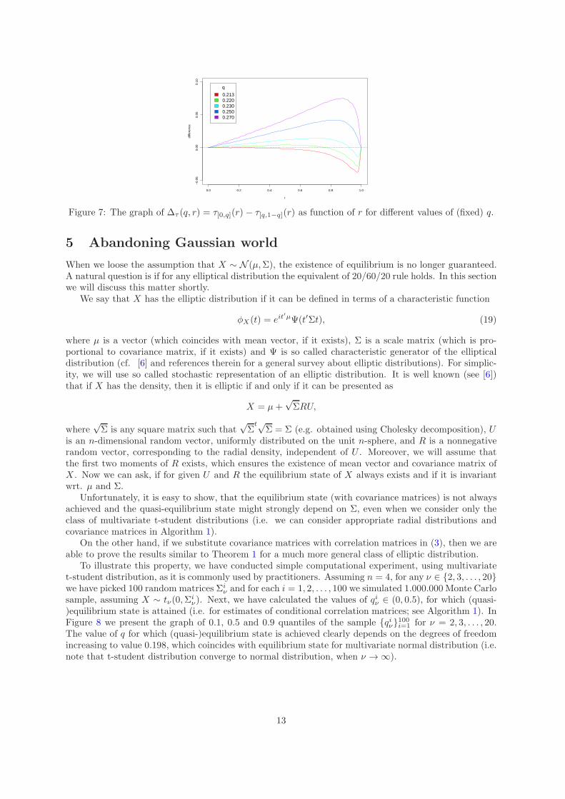
Figure 7: The graph of ∆τ (q, r) = τ[0,q](r) − τ[q,1−q](r) as function of r for different values of (fixed) q.

5 Abandoning Gaussian world

When we loose the assumption that X ∼ N (µ,Σ), the existence of equilibrium is no longer guaranteed.A natural question is if for any elliptical distribution the equivalent of 20/60/20 rule holds. In this sectionwe will discuss this matter shortly.

We say that X has the elliptic distribution if it can be defined in terms of a characteristic function

φX(t) = eit′µΨ(t′Σt), (19)

where µ is a vector (which coincides with mean vector, if it exists), Σ is a scale matrix (which is pro-portional to covariance matrix, if it exists) and Ψ is so called characteristic generator of the ellipticaldistribution (cf. [6] and references therein for a general survey about elliptic distributions). For simplic-ity, we will use so called stochastic representation of an elliptic distribution. It is well known (see [6])that if X has the density, then it is elliptic if and only if it can be presented as

X = µ+√ΣRU,

where√Σ is any square matrix such that

√Σ

t√Σ = Σ (e.g. obtained using Cholesky decomposition), U

is an n-dimensional random vector, uniformly distributed on the unit n-sphere, and R is a nonnegativerandom vector, corresponding to the radial density, independent of U . Moreover, we will assume thatthe first two moments of R exists, which ensures the existence of mean vector and covariance matrix ofX . Now we can ask, if for given U and R the equilibrium state of X always exists and if it is invariantwrt. µ and Σ.

Unfortunately, it is easy to show, that the equilibrium state (with covariance matrices) is not alwaysachieved and the quasi-equilibrium state might strongly depend on Σ, even when we consider only theclass of multivariate t-student distributions (i.e. we can consider appropriate radial distributions andcovariance matrices in Algorithm 1).

On the other hand, if we substitute covariance matrices with correlation matrices in (3), then we areable to prove the results similar to Theorem 1 for a much more general class of elliptic distribution.

To illustrate this property, we have conducted simple computational experiment, using multivariatet-student distribution, as it is commonly used by practitioners. Assuming n = 4, for any ν ∈ 2, 3, . . . , 20we have picked 100 random matrices Σi

ν and for each i = 1, 2, . . . , 100 we simulated 1.000.000 Monte Carlosample, assuming X ∼ tν(0,Σ

iν). Next, we have calculated the values of qiν ∈ (0, 0.5), for which (quasi-

)equilibrium state is attained (i.e. for estimates of conditional correlation matrices; see Algorithm 1). InFigure 8 we present the graph of 0.1, 0.5 and 0.9 quantiles of the sample qiν100i=1 for ν = 2, 3, . . . , 20.The value of q for which (quasi-)equilibrium state is achieved clearly depends on the degrees of freedomincreasing to value 0.198, which coincides with equilibrium state for multivariate normal distribution (i.e.note that t-student distribution converge to normal distribution, when ν → ∞).

13

Algorithm 1 Compute quasi-equilibrium state for elliptic distribution

Require:

n ∈ N+ – dimensionN ∈ N+ – size of Monte Carlo sampleradial.Dist – radial distribution (e.g.

√

χ(n) for multivariate normal)1: procedure Equilibrium(n,N ,radial.Dist)2: Generate U : N independent samples from n-dimensional unit sphere (uniform density)3: Generate R: N independent samples from (univariate) radial.dist4: Generate Σ = σij: n× n scale matrix (proportional to covariance matrix)

5: while

mini6=j

(

σ2ij/|σiiσjj |

)

< 0.2

∨

maxi6=j

(

σ2ij/|σiiσjj |

)

> 0.8

do

6: Generate (new) Σ = σij: n× n scale matrix7: end while

8: Compute√Σ, e.g. using Cholesky decomposition

9: Compute X = Xik = (√Σ)

′

RU (i.e. matrix n×N ; random sample from elliptic distribution)10: Define function Dist(q), for q ∈ (0, 0.5)11: function Dist(q)12: Compute q1, sample lower q-quantile of X1kNk=1

13: Compute q2 sample lower (1− q)-quantile of X1kNk=1

14: Compute conditional tail sample X1, by selecting all 1 ≤ k ≤ N , for which X1k ≤ q1

15: Compute conditional central sample X2, by selecting all 1 ≤ k ≤ N , for which q1 ≤ X1k ≤ q2

16: Compute Σ[0,q], a (conditional) covariance matrix of X1

17: Compute Σ[q,1−q], a (conditional) covariance matrix of X2

18: Compute d = ‖Σ[0,q] − Σ[q,1−q]‖F19: return d20: end function

21: Compute q = argmin0≤q≤0.5 Dist(q)22: return q23: end procedure

14

5 10 15 20

0.00

0.05

0.10

0.15

0.20

df

q

Figure 8: The graph of 0.1, 0.5 and 0.9 quantiles of qiν100i=1 for ν = 2, 3, . . . , 20.

Acknowledgments

Marcin Pitera acknowledges the support by Project operated within the Foundation for Polish ScienceIPP Programme ”Geometry and Topology in Physical Models” co-financed by the EU European RegionalDevelopment Fund, Operational Program Innovative Economy 2007-2013.

References

[1] Susan Annunzio, e-Leadership – Proven Techniques for Creating an Environment of Speed and Flexibility in

the Digital Economy, Human Resource Management 40 (2001), no. 4, 381–383.

[2] David Bach, Start late, finish rich: A no-fail plan for achieving financial freedom at any age, Crown Business,2005.

[3] B. Bolger, Ten steps to designing an effective incentive program, Employment Relations Today 31 (2004),no. 1, 25–33.

[4] James Creelman, An act of faith, The TQM Magazine 5 (1993), no. 3.

[5] David Dupper, School social work: Skills and interventions for effective practice, John Wiley & Sons, 2002.

[6] E. Gomez, M. A Gomez-Villegas, and J. M. Marın, A survey on continuous elliptical vector distributions,Revista matematica complutense 16 (2003), no. 1, 345–361.

[7] M. A. Grey and A. C. Woodrick, Latinos have revitalized our community: Mexican migration and Anglo

responses in Marshalltown, Iowa, New destinations: Mexican immigration in the United States (2005), 133–154.

[8] L. M. Hinman, The impact of the internet on our moral lives in academia, Ethics and information technology4 (2002), no. 1, 31–35.

[9] P. Jaworski and M. Pitera, On spatial contagion and multivariate GARCH models, Applied Stochastic Modelsin Business and Industry 30 (2014), no. 3, 303–327.

[10] N. L. Johnson, S. Kotz, and N. Balakrishnan, Continuous univariate distributions, vol. 1, 1994.

[11] A. Kamiya, F. Makino, and S. Kobayashi, Worker ants’ rule-based genetic algorithms dealing with changing

environments, Soft Computing in Industrial Applications, 2005. SMCia/05. Proceedings of the 2005 IEEEMid-Summer Workshop on, IEEE, 2005, pp. 117–121.

[12] R. B. Nelsen, An introduction to copulas, Springer, 2006.

[13] Les Robinson, A summary of diffusion of innovations, Enabling Change (2009).

[14] J. Slagell and J. Holtermann, Climbing peaks and navigating valleys: Managing personnel from high altitude,The Serials Librarian 52 (2007), no. 3-4, 271–275.

[15] Susan A Tynan, Best behaviors, Management Review 88 (1999), no. 10, 58–61.

15