PJ6400: Mobile Collector in Defense against Jamming Attack Written by: Lu Cui Supervised by: Natalija Vlajic, Andrew Eckford Abstract: A jamming attack on a wireless network is an attack in which the adversary attempts to cause a denial-of-service (DoS) by conducting simple, continuous or intermittent, transmission of high-power interfering signal. Wireless sensor networks (WSNs) are particular vulnerable to jamming attacks due to its natural characters. In our work, we propose to combat jamming attacks on WSNs through the deployment of mobile nodes. Specifically, we consider sending a mobile node inside the jammed area to periodically collect/sense data. Subsequently, the mobile is responsible for bringing the data to the most optimal exit point/node on the boundary of the attacked region. An algorithm named COEP is proposed for calculating the optimal exit point according to varies network conditions. 1. Introduction: A WSN (Wireless Sensor Network) is composed of a group of sensor nodes each capable of sensing and communicating. The sensor nodes used in WSNs are usually tiny and large scaled; moreover, they are typically battery powered. These nodes are deployed in a target field to form an ad-hoc network capable of reporting sensed data to the base station (Sink). WSN carries a wide range of applications, which can be further classified into monitoring applications and event tracking applications. For the tasks of monitoring, sensors periodically collect data from sensed environment, and report the collected sample to the Sink. Some examples are: environmental monitoring of air, water, oil; physiological monitoring of patients; condition maintenance in a factory etc. For tasks of event tracking, sensors capture the specific event happened in the target field, and take some action upon itself or by reporting to the sink. An example of event tracking application is the intrusion detection of security guarding. The design and operation of WSN involves many challenges due to its natural characters. One big challenge is node localization. Location awareness is important for WSNs since many applications such as mapping, object tracking depend on knowing the locations of sensor nodes. Moreover, location-based routing protocols, e.g. geographic routing, can save significant network resources by eliminating the need for route discovery broadcasting. Another challenge of WSN is the often ‘hostile’ environment of its deployed field. The deployed environment could be “hostile” in terms of the physical conditions, e.g. sensors are deployed into remote area with extreme temperatures to perform monitoring task. Or, it could also be ‘hostile’ in terms of the operational conditions, e.g. sensors are deployed in the presence of intentional jamming by an adversary. Besides the localization problem and the ‘hostile’ environment, another critical challenge in WSN is the constrained resources of sensor nodes. Since sensors are battery-powered in most applications, they are severely limited with energy supply. The limited energy level also restricts sensor’s network performance, such as node’s radio range, amount of data transmitted/processed, time spent in wake-up/idle/sleep mode, etc. To make matters worse, it’s often very difficult to change/recharge batteries for sensors due to the large scale of nodes or the hostile environment of deployed field. In fact, in many situations, i.e. forest fire-alarming sensors, old nodes are discarded when they run out of power. Regarding to the above-mentioned issues, reducing energy cost of sensor nodes is of great interest in WSNs. Other important challenges including deployment method, latency, throughput and bandwidth usage, etc. are also primary but are not discussed in detail here.

The rest of this article is organized as follows. Section 2 introduces the jamming attack in WSNs. In section 3, we propose to use mobile collector in combating jamming attack. An algorithm for calculating the optimal exit point of mobile collectors is also presented in this section. Section 4 carries the simulation details and Section 5 concludes this paper. 2. Jamming in Sensor Networks – Related Work A jamming attack on a wireless network is an attack in which the adversary attempts to cause a denial-of-service (DoS) by conducting simple, continuous or intermittent, transmission of high-power interfering signal. Wireless sensor networks (WSNs) are particular vulnerable to jamming attacks due to the following: (1) As no inter-nodal communication is possible inside the attacked region, the sensed data cannot be transmitted out of this region and, ultimately, delivered to the sink. (2) By exploiting the vulnerabilities of the link-layer, jamming attacks can force the nodes inside the attacked region to remain in the ‘wake up’ state over prolonged intervals of time. As a result, the nodes ‘under attack’ will quickly exhaust their energy/battery reserves and ‘die’. Jamming attacks are usually categorized by their jamming sources, i.e. constant jammer, deceptive jammer, random jammer, and reactive jammer [2]. The constant jammer continuously emits a radio signal, preventing sensor nodes from getting hold of the channel and sending packets. The deceptive jammer injects packets into the channel without any gap between subsequent packet transmissions. As a result, sensors are forced to remain in the receive mode, thus cannot send out packets. The random jammer alternates between sleeping phase and jamming phase, subsequently prolonged the jammer’s lifetime. And the reactive jammer stays quiet when the channel is idle, but starts transmitting radio signal as soon as the channel is active. Consequently, collision becomes standard in WSNs, and unnecessary retransmission increases exponentially. To date, only a handful of studies on the subject of jamming attacks in WSNs have been published. Some of the proposed anti-jamming radio techniques include: Channel-surfing, the use of transmission media likes Infrared or optical combined with radio [1]. The common disadvantages of these radio techniques are the requiring of extra radio devices installed on sensors, which ultimately causes extra expense and complexity. Besides the radio technologies, a mapping protocol named JAM is proposed by Woods in [3] to define the shape of the jammed area. JAM assumes that each node knows the location and unique ID of all its neighbors. And when jamming occurs, a node will broadcast a JAMMED message to its neighbors. Upon receiving a JAMMED message, the nodes on the boundary of the jammed region (but themselves are not jammed) will broadcast a BUILD message to its own neighbors to start building the jammed hole boundary. These “alive” nodes at the boundary will exchange and merge information describing which nodes they have witnessed as jammed. Eventually, the information of entire boundary is grouped together. We adopt JAM as a pre-request of our research. It should be noted that JAM is only suitable for static jamming attack, and this limit will also be the limit of our work. Another anti-jamming method is developed for mobile sensor network in [4], namely, spatial retreat. Spatial retreat is based on the following idea: Upon jamming, the mobiles nodes will carry the information out of the jammed area, and try to get reconnected with the rest of the network. And further more, when jammer leaves, the network will be restored. In [4], a method is developed for mobile nodes to escape from the jammed area. Specifically, after detecting itself as jammed, a node will choose a random direction to escape while, at the same time, running jamming detection algorithm. As soon the node leaves the jammed area, it moves along the boundary of the jammed area until it

reconnected to the rest network. Spatial retreat, in its original form, is shown to be very sensitive to the absence of any location information from the jammed area. Another disadvantage of this algorithm is the assumption that a large number of mobile nodes are present, i.e. available, in the network. With regard to these disadvantages, we propose to use mobile node in an opposite way of spatial retreat: to deploy a mobile collector into the jammed region. The idea of our proposed method is discussed in the following section. Conceptually, it is much less expensive and more efficient than spatial retreat. 3. Defense against Jamming by Means of a Mobile Collector 3.1 Introduction In defense against jamming attack, we propose to deploy a mobile collector into the jammed area to collect/sense data and periodically bring collected data out of the attacked region. The collector who moves through the jammed region can collect data from jammed nodes or simply sense data by its equipped sensors. One challenge of the mobile collector is to localize itself inside the jammed region. In this paper, we assume that the mobile is aware of the locations of itself and of the destinations through the use of GPS devices or other technologies. In addition, we also assume that a jammed area mapping protocol, e.g. MAP, is adopted such that the mobile is aware of the jamming boundary before it getting into the jammed area. Another challenge is the data-gathering manner of mobile collector. Author of [5] gives us some hint about efficient data gathering, specifically, the collector visits the collecting spots in the proportion of the node’s aggregate data rate (when collecting from jammed-nodes), but also with the goal of optimizing the distance traversed. One consequence of such scheme is that the collector’s last visited spot (before it ready to pass data to a boundary node) may vary with network context, e.g. node’s data rate etc. After gathering data, the last task for mobile collector is to efficiently pass collected data to a jamming boundary node and eventually to the Sink. The word ‘efficiently’ means fast, and with minimum energy cost. In our case, time is not critical since sensor nodes may collect data samples every few minutes and collector may take a long time to revisit a spot, e.g. every few hours [5]. Under such condition, the energy cost of both the mobile movement and the network transmitting is of the major concern. In another word, the mobile will manage to pass data to a boundary point that will best saves the mobile’s and network’s energy usage. Moreover, current network parameters such as mobile’s last position, mobile’s moving cost, amount of data to be transmitted etc, also affects the selection of the boundary node. In the next section, we propose a mathematical model for mobile collector to be able to calculate the optimal boundary point to pass data through.

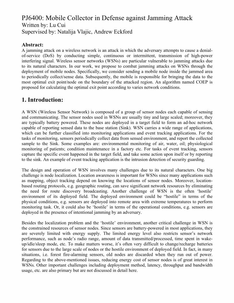
3.2 Mathematical Modeling of the Problem: The goal of our work is to find an optimal node on the boundary of a jamming hole (we will refer to this node as ‘optimal exit point’ – OEP) through which the mobile collector will pass data to the rest of the network and eventually to the sink. The selection of optimal exit point is aimed at minimizing the overall energy cost, which includes mobile moving/transmitting cost and the network transmitting cost. Our geometric model for calculating the OEP is derived as follows: (1) The jamming is assumed to caused by a single omnidirectional antenna. Consequently, the jamming area is modeled as a circular region of radius R. The center of the jamming region is annotated with O. Point O is also assumed to be the center of

Mobile(xm,ym) ‏rm R

X(x,y)

m

s1

s2

T(xtan,ytan) ‏

O(0,0)‏ Sink (xs, 0)‏ x

y

θ

N(R,0)

dr

P mP

Figure 1.b) Jamming area and the mobile: blue arrows indicate the data path when x≤xtan

y

Mobile(xm,ym) ‏

rm R m

T(xtan,ytan) ‏

O(0,0)‏ Sink (xs, 0)‏ x N(R,0)

dr

P mP

Figure 1.a) Jamming area and the mobile: blue arrows indicate the data path when x>xtan

S

X(x,y)

the coordinate system of the entire sensor network. The line passing through O and the sink is assumed to align with the x-axis, as illustrated in Figure 1.b). Note, Figure 1 shows only the upper half of the jamming region, as this half-area turn out to contain all elements necessary for our calculations. (2) A tangent line is drawn from the sink to the upper half of the jamming circle (Figure 1.b). The respective tangent point on the circle is annotated with T=(xtan, ytan). Here, we recognize that, relative to the tangent point T, the optimal exit point could fall into one of two possible regions - left or right of T. Consequently, a) If optimal exit point happens to be on the right-hand-side of tangent point T (i.e. xOEP≥xtan), data will be passed from the mobile to the exit point and then along a direct line to the sink, as illustrated in Figure 1.a). b) On the other hand, if optimal exit point happens to be on the left-hand-side of tangent point T (i.e. xOEP<xtan), data is passed firstly from the mobile to the exit point, then through an arc on the jamming circle, and finally along the tangent line to the sink (Figure 1.b)). (3) With regard to the mobile’s radio range (rm), we identify, and subsequently study, two possible scenarios. Scenario One): The mobile has a relatively short radio range and, from its initial location (xm, ym), it cannot reach any of the boundary points. Hence, to be able to pass data to any (including the optimal) exit point, the mobile needs to move first. Scenario Two): The mobile has a relatively long radio range and is able to pass data directly to a number of boundary points. In this case, depending on the actual location of the optimal exit point, it may or may not be necessary that the mobile moves from its initial location. Notations: Basic parameters affecting the result of optimization: xs: The distance between the center of the jammed region and the sink. R: The radius of the jamming hole. rm: Transmitting radius of the mobile node. In this work, we assume that

the radio range of the mobile is fixed and cannot be adopted (optimized) to a particular receiving point.

t: Data transmission time between any two transmitting nodes. (It’s assumed that static-to-static node transmission and mobile-to-static node transmission experience approximately the same transmitting time).

em: Energy consumed for the locomotion of the mobile per unit distance (i.e. per meter).

Pr: Minimum received signal power needed to reach the required limiting SNR.

Xm=(xm , ym): Initial location of the mobile node.

r: Radio range of a static node. K: Free space path loss parameter. K=Pt/(Pr*r2) where Pt is the

transmitting signal power. w: Weight factor indicates the level of importance of mobile energy cost

vs. network energy cost. Other notations and derived parameters:

X=(x, y): An arbitrary point on the jamming boundary (Figure 1). As such X represents the optimization variable of the problem, our goal is to find X, which minimizes the overall energy cost.

O=(0,0): Center of the jammed area (Figure 1). N=(R, 0): Point on the boundary of the jamming hole with the shortest physical

distance to the sink. P=(xP, yP): Point on the boundary of the jamming hole with the shortest physical

distance to the mobile. Given the fact that the minimum distance between a point (e.g. point M) inside a circle and the circle’s circumference is along the circle’s radius passing through M, xP can be calculated as xP=R*xm/(xm

2+ym2)1/2.

T=(xtan, ytan): Point on the boundary of the jamming region touched by the tangent line from the sink. Based on the properties of the right triangle formed by O, T and the location of the sink (see Figure 1.b)), the coordinates of T can be calculated as xtan=R2/xs and ytan=R*(xs2-R2)1/2/xs.

mP : The distance between the initial mobile location and point P, mp = R- (xm

2+ym2)1/2 (see Figure 1.b)).

m: The distance between the initial mobile location and X (see Figure 1.b)).

dr: The distance between the initial mobile location (xm , ym) and N, where dr = ((xm-R)2+ym

2)1/2 (see Figure 1.b)). s1: The length of the arc (on the boundary of the circle) between the X

and T (see Figure 1.b)). s2: The distance between the tangent point T and the sink (see Figure

1.b)). s: Minimum communication-path distance between X and the sink. As

illustrated in Figure 1.b), s comprises s1 and s2, hence s=s1+s2. 3.3 Analytical Search for Optimal Exit Point

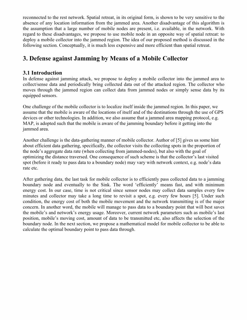
3.3.1 Scenario One: Mobile with a Short Radio Range:

Mobile(original) R

X(x,y)

O(0,0) ‏

Sink x

y

Fig.2. Mobile with short radio range

Mobile (after move)

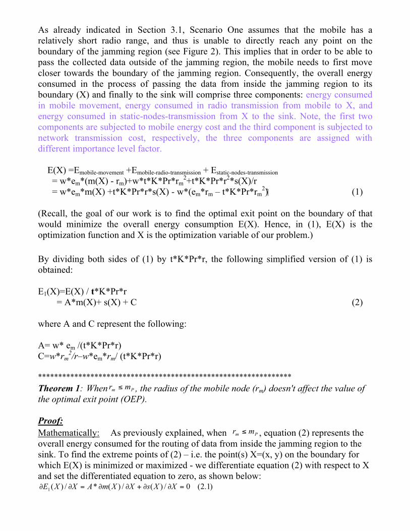
As already indicated in Section 3.1, Scenario One assumes that the mobile has a relatively short radio range, and thus is unable to directly reach any point on the boundary of the jamming region (see Figure 2). This implies that in order to be able to pass the collected data outside of the jamming region, the mobile needs to first move closer towards the boundary of the jamming region. Consequently, the overall energy consumed in the process of passing the data from inside the jamming region to its boundary (X) and finally to the sink will comprise three components: energy consumed in mobile movement, energy consumed in radio transmission from mobile to X, and energy consumed in static-nodes-transmission from X to the sink. Note, the first two components are subjected to mobile energy cost and the third component is subjected to network transmission cost, respectively, the three components are assigned with different importance level factor.

E(X) =Emobile-movement +Emobile-radio-transmission + Estatic-nodes-transmission = w*em*(m(X) - rm)+w*t*K*Pr*rm

2+t*K*Pr*r2*s(X)/r = w*em*m(X) +t*K*Pr*r*s(X) - w*(em*rm – t*K*Pr*rm

2) (1) ‏ (Recall, the goal of our work is to find the optimal exit point on the boundary of that would minimize the overall energy consumption E(X). Hence, in (1), E(X) is the optimization function and X is the optimization variable of our problem.)

By dividing both sides of (1) by t*K*Pr*r, the following simplified version of (1) is obtained: E1(X)=E(X) / t*K*Pr*r

= A*m(X)+ s(X) + C (2) where A and C represent the following: A= w* em /(t*K*Pr*r) C=w*rm

2/r–w*em*rm/ (t*K*Pr*r) *************************************************************** Theorem 1: When , the radius of the mobile node (rm) doesn't affect the value of the optimal exit point (OEP). Proof: Mathematically: As previously explained, when , equation (2) represents the overall energy consumed for the routing of data from inside the jamming region to the sink. To find the extreme points of (2) – i.e. the point(s) X=(x, y) on the boundary for which E(X) is minimized or maximized - we differentiate equation (2) with respect to X and set the differentiated equation to zero, as shown below:

Now, as C – the only term in equation 2.1 that contains rm – is completely independent of X, it gets fully omitted from the differentiated equation. As a result, rm also gets omitted from the differentiated equation and, ultimately, from the expression for the extreme points of (2). From the practical point of view this implies that the extreme points of (2), including the OEP that we are looking for, will not (and cannot) be affected by rm. Geometrically: With X being an arbitrary point on the jamming circle and Q the OEP when rm=0, let EX and EQ be the total energy consumed when the mobile exit from X and Q respectively1. Consequently, the following must hold,

. Now, if instead of rm=0 we assume that the mobile’s radio range (rm) takes some value in between 0 and mP, the following will also have to hold:

The added terms in equation 2.2 and 2.3 are due to two results of extending rm: a) mobile now consumes more energy in radio transmitting (2nd term in 2.2/2.3); b) Mobile now consumes less energy in moving (3rd term in 2.2/2.3). From the above equations, we further conclude:

Equation 2.4 clearly suggests that when 0< , Q is still the optimal exit point. Hence, the position of the optimal exit point, as defined in our optimization problem, does not depend on the actual value of rm. *************************************************** Through Theorem 2 we have proven that the mobile’s radio range (rm), as well as the entire parameter C=w*rm

2/r–w*em*rm/(t*K*Pr*r), can be omitted from the optimization equation (2), as they do not affect the extreme points of E(X). This further allows that in 11 Here we assume that the mobile physically moves all the way to the boundary of the jamming region and delivers data by using minimum (i.e. virtually zero) transmission energy.

the proceeding discussion we substitute the optimization function E(X) with Esimplified(X), as the extreme points of Esimplified(X) will fully match the extreme points of E(X). Esimplified(X)=A*m(X) + s(X) (3) Since the optimization variable X=(x, y) is a point on the jamming circle where y=(R2-x2)1/2, equation (3) can be expressed as a function of only one ‘unified’ variable - coordinate x. Moreover, it should be observed that boundary points on the left-hand-side of P (boundary points where x<xP - see Figure 1) could never be the OEP due to both of the extra mobile movement cost and static-transmission cost compared to P. Therefore, we get,

where

Note: when

(see Figure 1.b), where θ can

be calculated by applying “law of cosines” in the triangle formed by O, X and T:

To further simplify our analysis, we propose to normalize Esimplified(x) with respect to R, where R represents the radius of the jamming region (Figure 1). The main benefit of normalization is to further group the network parameters into smaller groups of factors. The resulting, normalized equation is shown below:

where

Note, the normalization implies that both sides of (4) are divided by R. Consequently,

XP-R, xtan-R and ytan-R in (5) corresponding to the normalized version of xP, xtan and ytan. That is, XP-R = XP/R, xtan-R=xtan/R, ytan-R=ytan/R. It should also be observed that the normalization with regard to R will not affect the relative position of the OEP on the jamming circle, and the OEP calculated from equation (5) will be the normalized version of the actual optimal exit point corresponding to (4), i.e. (2) and (1). For simplicity, we will use the same notation OEP to denote the normalized version of the OEP. The actual discussion on how to use (5) in order to find the OEP is provided in Section 3.4. We close this section by reminding the reader that, in addition to exit point X=(x,y), function (5) is also a function of 4 other parameters: A, xsR , and( xmR , ymR). For some of these parameters, the normalized equation (5) is non-convex and may have more than one local extreme (minimum or maximum). The global minimum point is selected among these extremes as the one carrying the minimum energy cost. 3.3.2 Scenario Two: Mobile with a Long Radio Range rm>mP In contrast to Scenario one, in Scenario two we assume the radio range of the mobile node is sufficiently long so that a direct communication between the mobile and some of the points on the boundary of the jamming circle is possible. Thus, the points on the jamming boundary can be split into two groups: points inside the mobile radio range and points outside the mobile radio range. In subsections S2.1) and S2.2), the energy

function corresponding to each of these two groups is studied separately. S2.1) Energy Function for Points inside Mobile’s Radio Range: If the mobile is to transmit data out of the jamming region and to the sink by passing it to one of the boundary points from this

group (points in the shaded area in Figure 3), the overall energy cost corresponding to such transmission would be: E(X) =Emobile-radio-transmission + Estatic-nodes-transmission = w*t*K*Pr*rm

2+t*K*Pr*r*s(X) (6) Where the first term indicts energy cost of radio transmission from mobile node to point X and the second term indicts the static-nodes-transmission cost from X to the sink. Now, it should be observed that for each point X in this region, the first term Emobile-radio-

transmission in (6) remains the same: w*t*K*Pr*rm2. Moreover, for X from this group that

Mobile R

O(0,0)‏ Sink x

y

Fig.3. Mobile with long radio range

rm

I

closest to the sink, the second term is the smallest, as it implies the smallest number of static nodes involved. Consequently, we conclude that out of the boundary points that happen to be inside the mobile’s radio range, the closer-to-sink intersection of the mobile radio circle and the jamming circle I (point XI=(xI, yI) in Figure 3) is the point that minimizes (6) and as such represents the local optimal exit point of the region in question. This point can be found simply by solving the system of two equations - the equation of jamming circle: (x2+y2 = R2), and the equation of the mobile radio circle: (x-xm)2+(y-ym)2=rm

2. Note, in an extreme case, the radio range of the mobile could extend beyond the right most jammed point N(R, 0) (if rm > dr). Under such conditions, the optimization problem becomes trivial, as the mobile could (would) just pass the data to the farthest static sensors it could reach along the way to sink.

S2.2) Energy Function for Points outside Mobile’s Radio Range: If the mobile is to transmit data out of the jamming region and to the sink by passing it to a node that happens to be outside of its radio range (e.g. node outside the shaded area in Figure 3), the respective energy cost of such transmission would entirely match that of Scenario one and equation (1): E(X) =Emobile-movement +Emobile--radio-transmission + Estatic-nodes-transmission (1) Notice that when X=I, where m=rm, the first term of equation (1) Emobile-movement becomes 0 which makes equation (1) the same as equation (6). In another word, I is the point where Scenario S2.1 and S2.2) ‘intersect with each other’ and also the point at which equations (1) and (6) ‘converge to each other’. (This is illustrated in Figure 4, where the dotted curve of E(x) on the left-hand-side of Ix corresponds to (6), whereas the solid curve of E(x) on the right-hand-side of Ix corresponds to (1). The two functions ‘meet’ at x=xI.) The given observation is of rather important practical significance. The observation implies that in order to find the global minimum of the energy function (i.e. to find the OEP), we only need to examine (1) on the region x≥xI. Namely, there is no need to examine (6) inside its respective domain (x≤xI), as (6) is proven to reaches its minimum at x=xI and this minimum happens to be of the same value as the value of (1) at x=xI. In the following section, we summarize the above two scenarios into one simple algorithm that can be adopted in calculating OEP for both cases.

Fig. 4.Energy functions when mobile has long radio radius Px

x

E(x)

Ix R

x

y

P

I

Mobile

rm

Eq.(1) Eq.(6)

3.4 Algorithm for Calculation of Optimal Exit Point (COEP) Based on the results of our analytical study from Section 3.3, here we propose a simple algorithm for calculation of optimal exit point (OEP), as has been defined in section 3.2. Step 1: Calculate the distance between the initial mobile location (xm, ym) and the

nearest boundary point P: mp = R- (xm2+ym

2)1/2

Step 2: If , calculate the OEP by finding the minimum of E(x) given in (5), with xR in the domain of [xP-R, 1].

Step 3: If rm>mP, calculate the OEP by finding the minimum of E(x) given in (5) with xR in the domain of [xI-R, 1], where point I is the closer-to-sink intersection of the mobile radio and the jamming hole.

Step 4: Calculate the actual coordinate of OEP by multiply R to the normalized result of OEP.

However, in this paper, we assume that the mobile node is able to obtain close-form solutions of the energy function by using pre-installed software, e.g. Matlab. In other cases, numerical estimation methods may be adopted by mobile node to calculate OEP. 3.5 Sensitivity Analysis To evaluate how the network-related parameters: R, r, A=w*em/(t*K*Pr*r) 2 affect the calculation, i.e. position, of the optimal exit point (OEP), in this section we first discuss the range of values that these parameters take in the real world. Subsequently, by keeping the parameters in the identified range, we investigate their individual impact on the energy function (5) and the position of the optimal exit point (OEP). 3.5.1 Real-World Parameter Values

1) The jamming radius: R. This parameter may vary from a few meters (cell phone jammer) to hundreds meters (portable bomb jammer) [7]. In our analysis, we will assume R to vary from 20-800m.

2) Mobile locomotion cost per meter: em. The movement energy consumption of a

surveyor SRV-1 robot [9] is about 10 joules/m, and of an Aerosonde aerial vehicle [8] is about 0.33J/m.

3) Sensor-to-sensor communication range: r. In the case of 900MHZ

2 These parameters appear in function (5) and, consequently, influence the position of the optimal exit point.

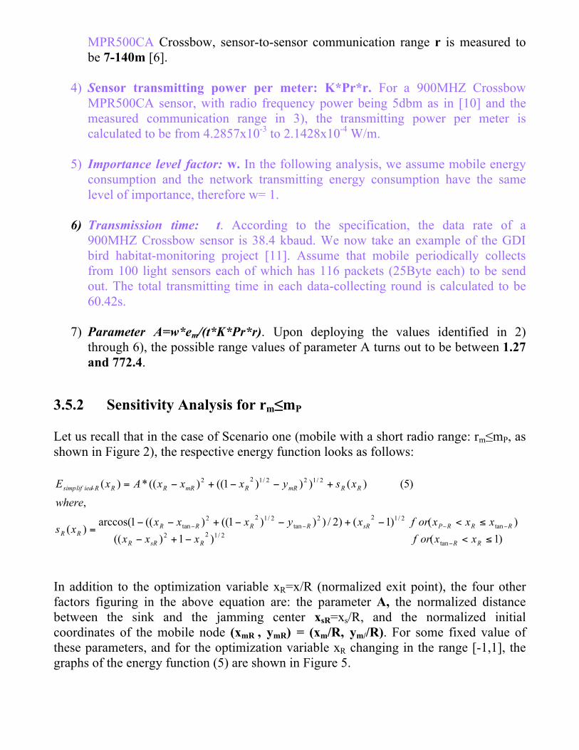
MPR500CA Crossbow, sensor-to-sensor communication range r is measured to be 7-140m [6].

4) Sensor transmitting power per meter: K*Pr*r. For a 900MHZ Crossbow

MPR500CA sensor, with radio frequency power being 5dbm as in [10] and the measured communication range in 3), the transmitting power per meter is calculated to be from 4.2857x10-3 to 2.1428x10-4 W/m.

5) Importance level factor: w. In the following analysis, we assume mobile energy

consumption and the network transmitting energy consumption have the same level of importance, therefore w= 1.

6) Transmission time: t. According to the specification, the data rate of a

900MHZ Crossbow sensor is 38.4 kbaud. We now take an example of the GDI bird habitat-monitoring project [11]. Assume that mobile periodically collects from 100 light sensors each of which has 116 packets (25Byte each) to be send out. The total transmitting time in each data-collecting round is calculated to be 60.42s.

7) Parameter A=w*em/(t*K*Pr*r). Upon deploying the values identified in 2)

through 6), the possible range values of parameter A turns out to be between 1.27 and 772.4.

3.5.2 Sensitivity Analysis for rm≤mP Let us recall that in the case of Scenario one (mobile with a short radio range: rm≤mP, as shown in Figure 2), the respective energy function looks as follows:

In addition to the optimization variable xR=x/R (normalized exit point), the four other factors figuring in the above equation are: the parameter A, the normalized distance between the sink and the jamming center xsR=xs/R, and the normalized initial coordinates of the mobile node (xmR , ymR) = (xm/R, ym//R). For some fixed value of these parameters, and for the optimization variable xR changing in the range [-1,1], the graphs of the energy function (5) are shown in Figure 5.

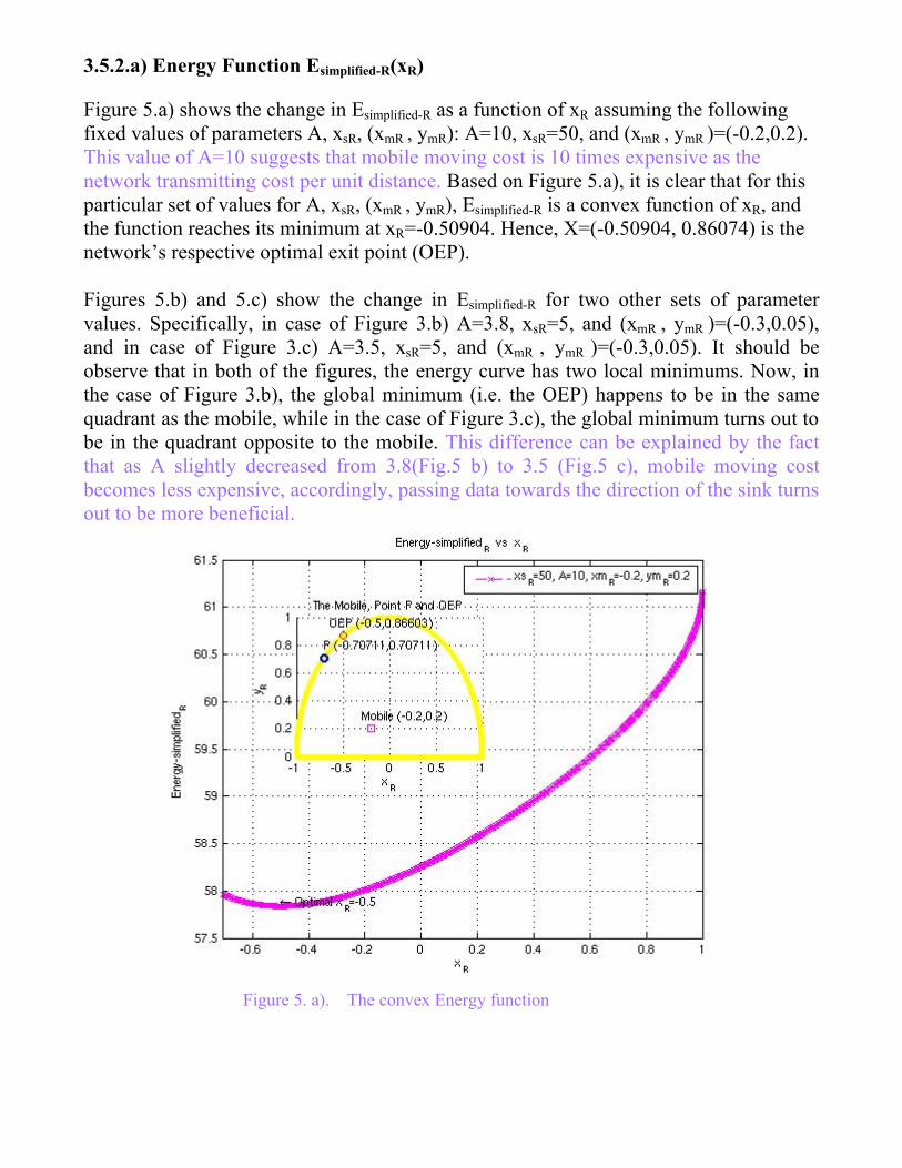
3.5.2.a) Energy Function Esimplified-R(xR) Figure 5.a) shows the change in Esimplified-R as a function of xR assuming the following fixed values of parameters A, xsR, (xmR , ymR): A=10, xsR=50, and (xmR , ymR )=(-0.2,0.2). This value of A=10 suggests that mobile moving cost is 10 times expensive as the network transmitting cost per unit distance. Based on Figure 5.a), it is clear that for this particular set of values for A, xsR, (xmR , ymR), Esimplified-R is a convex function of xR, and the function reaches its minimum at xR=-0.50904. Hence, X=(-0.50904, 0.86074) is the network’s respective optimal exit point (OEP). Figures 5.b) and 5.c) show the change in Esimplified-R for two other sets of parameter values. Specifically, in case of Figure 3.b) A=3.8, xsR=5, and (xmR , ymR )=(-0.3,0.05), and in case of Figure 3.c) A=3.5, xsR=5, and (xmR , ymR )=(-0.3,0.05). It should be observe that in both of the figures, the energy curve has two local minimums. Now, in the case of Figure 3.b), the global minimum (i.e. the OEP) happens to be in the same quadrant as the mobile, while in the case of Figure 3.c), the global minimum turns out to be in the quadrant opposite to the mobile. This difference can be explained by the fact that as A slightly decreased from 3.8(Fig.5 b) to 3.5 (Fig.5 c), mobile moving cost becomes less expensive, accordingly, passing data towards the direction of the sink turns out to be more beneficial.

Figure 5. a). The convex Energy function

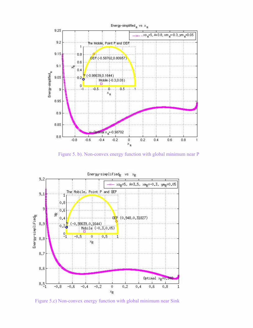
Figure 5. b). Non-convex energy function with global minimum near P

Figure 5.c) Non-convex energy function with global minimum near Sink

3.5.2.b) OEP as a Function of A With regard to some specific value of xsR and xmR, ymR, if we derive OEP from equation (5) for each value of A within a certain range, we can plot OEP as a function of A. Fig. 6 is such a graph showing the change of OEP as A increases from 1 to 100 by assuming xsR=50 and (xmR , ymR )=(-0.2,0.2). Note the weight factor A=w*em/ (t*K*Pr*r) is the ratio of mobile-moving expensiveness vs. network-transmitting expensiveness. We observe from Fig.6 that as A increase, the corresponding OEP is getting closer to point P (the nearest boundary point) and vise versa. This is because larger value of A suggests that mobile moving is costly, therefore, it's more beneficial to “move less” in order to minimize the overall energy cost. On the other hand, smaller value of A suggests that it is more beneficial to move towards the direction of sink in order to short the network-transmitting path.

Fig 6. OEP as a function of A

3.5.2.c) OPE as a Function of xs-R Again, by assuming A=3 and (xmR , ymR )=(0.1,0.2), Fig 7 derives the corresponding OEP from equation (5) for each value of xsR in between 1 to 150. As xsR indicts how far is the sink away from the jamming center, we observe that as sink getting farther away, OEP eventually reaches a steady point. This steady point is determined by the value of A

together with mobile initial location.

Fig. 7. OEP as a function of xsR 3.5.2.d) OPE as a Function of (xm-R, ym-R) - Region of Sensitivity

In the following graph we capture the percentage of energy saved when the mobile transmits data out of the jamming hole by passing it through P rather than OEP. (Note, P is the point on the boundary of the jamming hole physically closes to the sink and is easy to identify - see Section 3.2. The OPE, on the other hand, needs to be identified using the COPE algorithm outlined in Section 3.4.) Specifically, Figure 8 shows the percentage of saved energy psaved:

psaved(xm-R, ym-R)= (EP-EOEP)/EP. as a function of the initial coordinates of the mobile. Please note that the plot in Figure 8 has been derived assuming a relatively small value of XsR=2. Namely, for large values of xs-R, the majority of energy cost corresponds to the transmission of data between the jamming boundary and the sink3, and the actual choice of the exit point does not have a significant impact. Only for relatively small values of 3 A large xs-R implies a far-away sink

Xs-R (such as Xs-R =2), the actual choice of the exit point will have a clearly observable effect on the energy cost. From the practical point of view, Figure8.a) implies that if the mobile happens to be initially located around the left side of jamming center, exiting from the OEP will save a big percentage of energy, i.e. psaved(-0.1, 0.5)=28%. Otherwise, if the mobile happens to be initially located close to the jamming boundary, the energy saved by utilizing the OEP is very small, i.e. psaved(-0.1, 0.8)<1%. We define the mobile initial locations where exiting from OEP and P have non-negligible difference - the “region of sensitivity”. Figure 4.b) further shows that the region of sensitivity is greatly affected by the value of parameter A. Namely, as the value of A increases from 3 to 10, the resulted region of sensitivity shrinks to a very small region – as shown in Figure 4.b). This is due to the fact that a large A implies generally costly mobile movement. Consequently, in order to minimize the mobile-movement related energy cost (which for big A represents the biggest component of the overall energy cost), the OEP is chosen very close to P. Practically, the results of Figure 8 can be summarized as follows: From the perspective of the overall energy consumption, passing data through the point on the boundary physically closes to the mobile node (P) is as effective as passing data through the OEP (which needs to be calculated using COEP algorithm of Section 3.4), except in the following two cases: 1) The value of parameter A is small, or 2) The mobile initially resides near the centre of the jamming region.

Figure 8.a) Region of sensitivity when A=3

Figure 8.b) Region of sensitivity when A=10

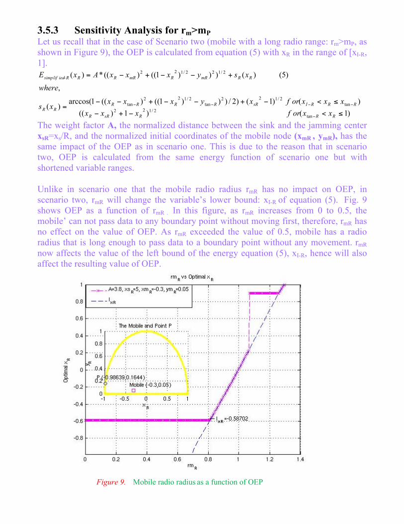
3.5.3 Sensitivity Analysis for rm>mP Let us recall that in the case of Scenario two (mobile with a long radio range: rm>mP, as shown in Figure 9), the OEP is calculated from equation (5) with xR in the range of [xI-R, 1].

The weight factor A, the normalized distance between the sink and the jamming center xsR=xs/R, and the normalized initial coordinates of the mobile node (xmR , ymR), has the same impact of the OEP as in scenario one. This is due to the reason that in scenario two, OEP is calculated from the same energy function of scenario one but with shortened variable ranges. Unlike in scenario one that the mobile radio radius rmR has no impact on OEP, in scenario two, rmR will change the variable’s lower bound: xI-R of equation (5). Fig. 9 shows OEP as a function of rmR . In this figure, as rmR increases from 0 to 0.5, the mobile’ can not pass data to any boundary point without moving first, therefore, rmR has no effect on the value of OEP. As rmR exceeded the value of 0.5, mobile has a radio radius that is long enough to pass data to a boundary point without any movement. rmR now affects the value of the left bound of the energy equation (5), xI-R, hence will also affect the resulting value of OEP.

Figure 9. Mobile radio radius as a function of OEP

4. Simulation In this section, we evaluate the performance of COEP algorithm using the OPNET simulator. 4.1 Simulation Environment The constructed network as shown in Fig 10 contains a mobile collector, a sink and several router nodes. The router nodes are arranged into a half circle to model the boundary points of a jamming hole. Initially, the traffic is generated at mobile node0. Subsequently, mobile node0 will move towards a selected boundary node until it’s able to pass data to that node. Eventually, data will be routed through the rest boundary nodes all the way to the sink.

Fig. 10. Network structure

4.2 Simulation Result Taking the example of the habitat-monitoring project in [11], we assume that there are 100 Crossbow 900Hz MPR500CA sensor nodes each carrying 116 packets (25Byte) to be collected in a jammed region of radius 400m. We also assume an Aerosonde aerial vehicle [8] is adopted as the mobile collector. According to these assumptions, the network parameters are as following: jamming radius R=400m; sink distance from the jamming center, xs=600m; mobile moving cost per meter: em=0.33J/m; data transmitting time t=60s; radio range of sensors: r=30m; sensor transmitting power per meter: K*Pr*r = 0.001w/m. With these specific value of parameters, the calculated weight factor A=5.5, which is a relative small number indicates mobile moving is as 5.5 times expensive as network transmitting. If mobile is initially located at xm=-80m, ym=40m, the nearest node on the

boundary is node 25 in Fig.10, and the calculated OEP from COEP algorithm is node 20 in Fig. 10. The simulated result in Fig 11 compares the energy cost of mobile collector passing data from OEP (the red curve) and from P (the blue curve) respectively. Initially, more energy is consumed by moving to OEP rather than P. But eventually, transmitting through OEP over performs transmitting from point P.

Fig.11 Energy consumed by passing data from P and OEP 5. Conclusions In this paper, we proposed to use mobile collector in defense against jamming attack in WSNs. We also proposed an algorithm, namely COEP, for calculating the optimal boundary nodes that mobile collector will pass data to. More, these proposed schemes are suitable for any circular shaped holes in WSNs, e.g. coverage holes, routing holes etc. The simulation result shows that by passing data through the calculated optimal boundary node, the overall energy cost of delivering data from mobile collector to the sink is greatly saved.

Reference: [1] N. Ahmed, S. S. Kanhere, and S. Jha, “The holes problem in wireless sensor networks: a survey”, SIGMOBILE Mob., Comput. Commun. Rev., vol. 9, no. 2, pp. 4–18, 2005.

[2] Wenyuan Xu, Ke Ma, Wade Trappe and Yanyong Zhang, “Jamming Sensor Networks: Attack and Defense Strategies”, IEEE, Network, 2006 [3]Anthony D. Wood, John A. Stankovic, and Sang H.Son, “ JAM, A Jammed-Area Mapping Service for Sensor Network”,proc. IEEE international RT System,2003 [4]Ke Ma, Yangyong Zhang, Wade Trappe, “Mobile Network Management and Robust Spatial Retreats Via Network Dynamics” Proc.. 1st Int’l. Wksp Resource Provisioning and Mgmt. In Sensor Networks, 2005 [5] Y Tirta, Z Li, YH Lu, S Bagch, “Efficient collection of sensor data in remote fields using mobile collectors” 13th International Conf. on Comp. Comm. and Networks, IEEE Cat. No.04EX969 pp.515-519).”, [6]R.A.Alhameed, K.V.Horoshenkov, Y.F.Hu “Measure the range of Sensor Network”, http://www.mwrf.com/Articles/Index.cfm?Ad=1&Ad=1&Ad=1&ArticleID=19915 [7]Radio jammer. [Online] http://www.anci-group.com/Radio_Jammer.html [8] NASA. Aerosonde unmanned aerial vehicle, manufactured by aerosonde robotic aircraft limited. URL:http://uav.wff.nasa.gov/UAVDetail.cfm?RecordID=Aerosonde. [9] (2008) Surveyor Corporation. [Online]. http://www.surveyor.com [10] Wireless Sensor Network. [Online]. http://www.xbow.com/ [11] A. Mainwaring, J. Polastre, R. Szewczyk, and D. Culler. “Wireless sensor networks for habitat monitoring”, In ACM Workshop on Sensor Networks and Applications, 2002.