planning models and techniques
TRANSCRIPT

UNIT 5
PLANNING MODELS AND TECHNIQUES
The present unit contains major planning models concerning the use of investment criterion. The unit contains input-output analysis in lesson-1, linear programming in lesson-2, social accounting matrix in lesson-3, computable general equilibrium model in lesson-4, cost-benefit analysis in lesson-5 and logical framework approach in lesson-6. The linkages or inter-relationships between different production sectors and industries are extremely important for formulating a consistent plan. Input-Output analysis can capture such linkages. Social accounting matrix (SAM) which includes institutions that make up the economy (e.g. firms, households, government) in the output model table and hence gives a more comprehensive account of the economy. The linear programming which uses similar information as the two previous models in order to arrive at the optimal allocation of resources for the economy for a given objective function. Project appraisal is the most microeconomic and most commonly employed tool of planning. Project appraisal is based on the theory of social cost-benefit analysis. The purpose of logical framework (or logframe) approach is to undertake participatory, objectives-oriented planning that spans the life of project or policy work to build stakeholder team commitment and capacity with a series of workshops.

School of Business
Economic Development and Planning Page-236
Blank Page

Bangladesh Open University
Unit-5 Page-237
Lesson 1: Planning, Input-Output Models Objectives
After studying this lesson, you will be able to: Use input-output analysis Form input-output table Explain the general solution of input-output model Explain the limitations of input-output model
Planning In free market economy, according to theory, resources are allocated by the ‘invisible hand’ of the market in accordance with consumed demand. The theory says that market prices act as signals to producers, consumers consume till marginal utility equals price and producers produce to the point where marginal cost is equal to the price. Thus, theory postulates that resources will be optimally allocated since the marginal utility of production will just equal the marginal cost. There are many problems of the postulation in real life.
Planning in different forms has been accepted as an important policy instrument to attain specific targets.
The case for planning:
State intervention in the form of planning is necessary since the factor and product markets in the developing economies are imperfect and may not lead to efficient allocation of resources.
As private investors are less likely to provide much attention to the dynamic externalities generated in the process of development and difference between marginal net social benefit (MNSB) and private net private benefit (MNPB), planning may intervene to remove differences between MNSB& MNPB.
In the pursuance of goal of maximising profit in the short-run, the private investors may lead to a resource allocation which may not be socially optimal.
It is argued that planning may intensify acceleration of the developing countries task of achieving of higher growth path.
Planning may exert and create conditions for institutional and structural reforms which act as determinant of achieving rapid economic growth.
Planning may prove to be better alternative for the most productive use of limited resources of the developing economies.
The case against planning:
If planning envisaged necessary for market imperfections, the task should be to remove imperfections in the market, not planning.

School of Business
Economic Development and Planning Page-238
For removing the differences between MNSB &MNPB, the best alternative are either imposition of tax or granting of subsidies.
Given the lack of efficient human resources to tackle planning and wider spread intervention of the state,, an inefficient and corrupt bureaucracy may increase waste of resources that otherwise could have avoided.
The planning, by way of intervention, may lead to creating distortions in the market.
Despite such arguments for and against economic models are frequently used to construct economic planning with a view to: achieve consistency between demand and supply in different sectors; comprehend whether investment demand is enough to produce a
target output; determine intermediate demands for inputs including capital and
labour; enable the planner to test the feasibility and optimality of different
projects with a plan.
Input-Output Analysis
Input-Output (I-O) analysis is frequently used as an aid to development planning. The I-O analysis records or measures the transactions in respect of inputs needed for the output. Wassily Leontief 1used the first input-output tables for United States for the year 1919 to 1929 which earned him Nobel prize in 1973.
Input-Output (I/O) table captures the economy by dividing it into sectors and tracing the flow of inter-industry purchases (inputs) and sales (outputs). The I-O table presented in matrix form shows the distribution of output horizontally along its rows, and the composition of inputs vertically down its columns.
The fundamental idea of the I-O analysis may be illustrated with the example of computer. For the simplicity, it is assumed that production of computer requires hardware and software. Now assume an increase in the demand for computer. This will require an increase in output of the related industry – hardware and software and in other industries too. For example, an increase in the demand for hardware means changes in the production of motherboard, processor, cables, cases, electric ware, etc. And so and so forth. In the I-O analysis, all changes – direct, indirect or induced – are accounted to predict the total output of various inter-linked activities to meet a given changes in the demand for a product.
1 Leontief W. W. (1951), The Structure of the American Economy, New York: Oxford

Bangladesh Open University
Unit-5 Page-239
The Uses of Input-Output Analysis
The Input-Output analysis is useful in several ways. The various ways of use of the tool is described below:
Input-output analysis may have used for projection and forecasting purposes. After some manipulation an inter industry transaction matrix can provide information on how much of commodities X1, X2, etc. will be required at some future date assuming a certain growth rate of national income or final demand. Information of this nature is important if planning is to achieve consistency and if future bottlenecks in the productive process are to be avoided.
Input-output analysis can be used for simulation purpose. The simulation of development is concerned with what is economically feasible, as opposed to forecasting, which is concerned with what one expects to happen on the basis of a certain set of assumptions. With some manipulation, the inter-industry transactions matrix can be used for providing answers to such questions as: how will the production requirements of the economy be altered if a new steel mill is introduced; or what will be the repercussions on the economy if a series of import-saving schemes are introduced?
The I-O analysis can be used to: forecast import requirements and the balance of payments effects
of given changes in the final demand. forecast investment requirements consistent with a given growth
target if information is available on incremental capital-output ratios.
calculate the matrix multiplier attached to different activities; that is, the direct and indirect effects on the total output of all activities in the system from a unit change in the demand for the output of any one activity.
show the strength of linkages between activities in an economy. illustrate the technology of an economy.
Input-Output framework
The basics of input-output framework and some of its economic implications are discussed in the section. In order to make use of I-O method, certain simplifying basic assumption are to be made. These are as under:
No substitution takes place between the inputs to produce a given unit of output and input coefficients are constants. The linear input functions imply that the marginal input coefficients are equal to the average.
Joint products are ruled out, i.e. each industry produces only one commodity and each commodity is produced by only one industry.
School of Business
Economic Development and Planning Page-240
External economics are ruled out and production is subject to the operation of the constant returns to scale.
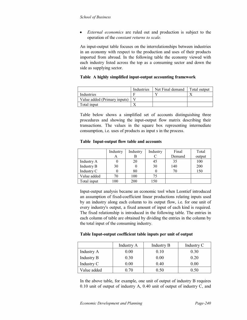
An input-output table focuses on the interrelationships between industries in an economy with respect to the production and uses of their products imported from abroad. In the following table the economy viewed with each industry listed across the top as a consuming sector and down the side as supplying sector.
Table A highly simplified input-output accounting framework Industries Net Final demand Total output Industries F Y X Value added (Primary inputs) V Total input X Table below shows a simplified set of accounts distinguishing three procedures and showing the input-output flow matrix describing their transactions. The values in the square box representing intermediate consumption, i.e. uses of products as input s in the process. Table Input-output flow table and accounts
Industry A
Industry B
Industry C
Final Demand
Total output
Industry A Industry B Industry C
0 30
0
20 0
80
45 30
0
35 140
70
100 200 150
Value added 70 100 75 Total input 100 200 150 Input-output analysis became an economic tool when Leontief introduced an assumption of fixed-coefficient linear productions relating inputs used by an industry along each column to its output flow, i.e. for one unit of every industry's output, a fixed amount of input of each kind is required. The fixed relationship is introduced in the following table. The entries in each column of table are obtained by dividing the entries in the column by the total input of the consuming industry. Table Input-output coefficient table inputs per unit of output
Industry A Industry B Industry C Industry A Industry B Industry C
0.00 0.30 0.00
0.10 0.00 0.40
0.30 0.20 0.00
Value added 0.70 0.50 0.50 In the above table, for example, one unit of output of industry B requires 0.10 unit of output of industry A, 0.40 unit of output of industry C, and

Bangladesh Open University
Unit-5 Page-241
generates 0.50 unit of value added. Thus in order to produce output XA, XB and XC, the amount of product A (out of industry A) required as intermediate input is equal to (1.1) 0.00XA - 0.00XB - 0.00XC Equation 1.1 calculates the total amount of product A used as intermediate input in the production process of an economy. If the remaining value of the same product left for net final demand, i.e., 35 in table 1.2 is further added to intermediate consumption, the total output of industry A is obtained in equation 1.2. (1.2) 0.00XA - 0.00XB - 0.00XC + 35 = 100 It is possible to check the equality property of equation 1.2 by replacing the values of XA, XB and XC in table 1.2 by their actual values. the results are shown in equation 1.3. (1.3) 0.00 X (100) - 0.10 X (200) - 0.30 X (150) + 35 = 100 The utilisation of products B and C as intermediate inputs of production may be similarly calculated. In general, the ratios shown in the box in table 1.2 could be written in more abstract terms, such as those in table 1.4, so that an input-output model may be formulated. Table 1.4 Input-output coefficient table in more general terms Industry 1 Industry 2 Industry 3 Industry 4 Industry 1 Industry 2 Industry 3
a11
a21
a31
a12
a22
a32
a13
a23
a33
Y1
Y2
Y3 Value Added V1 V2 V3 The relationship in equations 1.1, 1.2, 1.3 using general terms of table 1.4 can be shown as follows:
a11X1 + a12X2 + a13X3 + Y1 = X1
a21X1 + a22X2 + a23X3 + Y2 = X2 (1.4) a31X1 + a32X2 + a33X3 + Y3 = X3
In matrix form, equation 1.4 can me written as follows:
a11 a12 a13 X1 Y1 X1
a21 a22 a23 X X2 + Y2 = X2 (1.5) a31 a32 a33 X3 Y3 X3 In a more general form with n industry and n product, where a11 stands for input i (products of industry i) used in the production of one unit of output on industry j, systems of equations 1.4 and 1.5 can be written as follows:

School of Business
Economic Development and Planning Page-242
a11X1 + a12X2 + ...... + a1nXn + Y1 = X1
a21X1 + a22X2 + ...... +a2nXn + Y2 = X2 (1.6) + + + + a31X1 + a32X2 + ...... +a3nXn + Y3 = X3
and in matrix form a11 a12 a1n X1 Y1 X1
a21 a22 a2n X X2 + Y2 = X2 (1.7) .................. .... ... ... an1 an2 ann Xn Yn Xn
The computation of the coefficient matrix can be described in the following mathematical form:
Fij
aij =
Xy
where Fij stands for an element of the flow table as described in a square box of table 1.1 equation 1.7 is usually written from, as (1.8) AX + Y = Y Relationship 1.8 is the basic input-output system of equations. Matrix A is called the input-output coefficient matrix, vector X is the vector of output and vector Y is the vector of net final demand. The dimension (size) of matrix A is constrained only by the statistical information on inputs and outputs available to statistics since some countries have constructed input-output tables up to almost 500 industries. The limitations of the use of the IO model: There is no doubt about the usefulness of the I-O tool for development planing, but it also suffers from some limitations. This is particularly so in the less-developed countries. First, the IO analysis assumes that the input coefficients would remain unchanged. However, these coefficients may not remain constant when growth is taking place. In the long run the validity of the assumption of a constant coefficient is all the more questionable as technical progress gains momentum, substitution possibilities and returns to scale might be rising instead of being constant. Marginal input coefficients might no longer be equal to the average. Second, if the linkages among the different sectors are rather weak or non-existent, then the IO table will provides only very limited information.

Bangladesh Open University
Unit-5 Page-243
Third, the IO analysis assumes that the composition of demand is constant. In the long-run this is unlikely to be valid and any change in demand composition is likely to impact upon input coefficients. However, it should be pointed out that some of these limitations in the application of the IO analysis can be removed by continuously updating the IO tables to incorporate any effects of change in technical progress and/or demand pattern on sectoral input coefficients. Also if the IO analysis is used to make short, rather than long run predictions, and if the data are reliable, then the margin of errors is unlikely to be large. Finally, the IO analysis further assumes that each industry has only one, way of producing; a given product. But it is conceivable that there could be more than one process or activity to produce a commodity. IO analysis cannot help to find out which process among two or more activities would use the minimum amount of resources. In short, IO analysis cannot help to solve the choice of optimal technique of production.

School of Business
Economic Development and Planning Page-244
Questions for review 1. Input-output model was first developed for
A. UK B. Australia C. Bangladesh D. USA
2. Input-output model has the best use in
A. Preparing Budget B. Preparing plans C. Review annual production of a firm D. Calculate profit ad loss of an economy
3. Lentief won Nobel Prize in
A. 1919 B. 1929 C. 1968 D. 1973
Answer 1.D, 2.B, 3.D, Short Questions 1. What does input-output table show? 2. What are the major purposes of the input-output analysis? 3. What are the limitations of input-output analysis? Essay type questions
1. Explain the statement that there is no doubt about the usefulness of the I-O tool for development planning, but it suffers from serious limitations.
2. Construct a simple I-O table for a hypothetical country. Further Readings: 1. Dervis, K., Melo, J. and Robinson, S., General Equilibrium Model
for Development Policy, The World Bank, Washington D.C., 1982. 2. Arrow,K., S. Karlin, and P. Suppes,eds., Mathematical Methods
in Social Sciences, Standford, Califf., Standford University Press, 1960.

Bangladesh Open University
Unit-5 Page-245
3. Bacharach, M., Biproportional Matrices and Input-Output Change, Cambridge: Cambridge University Press, 1970.
4. Carter, A., and A. Brody, eds., Contribution to Input-Output Analysis, Amsterdam: North Holland, 1970.
5. Polenske,K. R. and J. Skolka, eds., Advances in Input-Output Analysis, Cambridge, Mass.:Ballinger, 1976.
6. Peacock A T and Dosser, D, “Input-Output Analysis in An Underdeveloped Country: A Case Study,” Review of Economic Studies, October, 1957.
7. Thirlwall A.P., Growth and development, Macmillan, 1994 8. Todaro M, Economic Development, Addison Wesley Longman pte
Ltd., 2001 9. Kasliwal P, Development Economics, South Western College
Publishing., 1995 10. Lal A N K, Economics of Development and Planing, Vikas
Publishing House Pvt. Ltd., 1997 11. Allen, R. G. D., Mathematical Economics, London, Macmillan,
1960.

School of Business
Economic Development and Planning Page-246
Appendix-1: Input-Output Analysis using Matrix Basic assumption of the input-output analysis No substitution takes place between the inputs to produce a given unit
of output and input coefficients are constants. The linear input functions imply that the marginal input coefficients are equal to the average.
Joint products are ruled out, i.e. each industry produces only one
commodity and each commodity is produced by only one industry. External economics are ruled out and production is subject to the
operation of the constant returns to scale. The above assumptions require that to produce one unit of the jth good, the required ith input would be constant and let us call it aij. Thus the production of each unit of the ith good would need, say a1j of the first commodity, a2j of the second , and a nj for the nth input. Here note that the first subscript refers to the input and the second one refers to the output. Hence if aij = 0.20 paisa , it means that 20 paisa worth of the ith commodity is necessary as an input to produce a 1 taka worth of the jth good. The symbol aij is regarded as the input coefficient. Let there be n number of industries in the economy. The input output table in the form of a matrix A=[aij] would state the input coefficients. So the availability of the input-output table is thus an important condition for any calculation. Actually the table shows the inter industry flows where each column shows the necessary input for producing one unit of output of a certain industry. If any element in the matrix is zero, it shows that the input demand is zero. The input coefficient can be written as:
aij = XjXij
i= 1,2,……..,n
j = 1,2,……..,n where Xj = total output of the jth industry Xij= number of units of ith goods used by jth industry. The IO table usually given in the following matrix:
Bangladesh Open University
Unit-5 Page-247
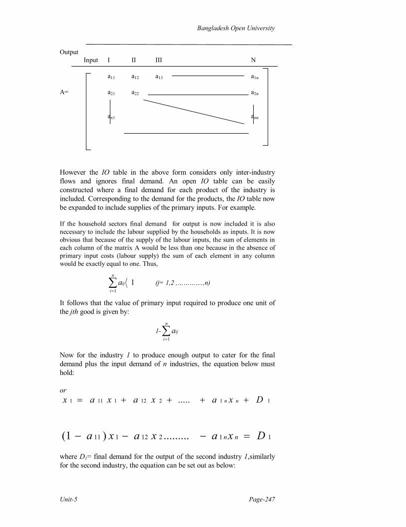
Output Input I II III N a11 a12 a13 a1n A= a21 a22 a2n
an1 ann However the IO table in the above form considers only inter-industry flows and ignores final demand. An open IO table can be easily constructed where a final demand for each product of the industry is included. Corresponding to the demand for the products, the IO table now be expanded to include supplies of the primary inputs. For example. If the household sectors final demand for output is now included it is also necessary to include the labour supplied by the households as inputs. It is now obvious that because of the supply of the labour inputs, the sum of elements in each column of the matrix A would be less than one because in the absence of primary input costs (labour supply) the sum of each element in any column would be exactly equal to one. Thus,
11
n
iija (j= 1,2 ,………….,n)
It follows that the value of primary input required to produce one unit of the jth good is given by:
1-
n
iija
1
Now for the industry 1 to produce enough output to cater for the final demand plus the input demand of n industries, the equation below must hold: or
112121111 ..... Dxaxaxax nn
11212111 .........)1( Dxaxaxa nn where D1= final demand for the output of the second industry 1,similarly for the second industry, the equation can be set out as below:

School of Business
Economic Development and Planning Page-248
22222121 .........)1( Dxaxaxa nn Thus
nnnnnn Dxaxaxa )1(.....2211 The system of equation can be written as in the following matrix form: (1-a11) -a12 -a1n x1 D1 -a21 (1-a22) -a2n x2 D2 (I-A)x = = -an1 -an2 (1-ann) xn Dn where the identity matrix is given by: 1 0 0 0 0 1 0 0 1=
0 0 0 1 that is, all the elements in the principal diagonal are 1and elsewhere zero. Now solving for x, we have:
DAx 11 The rule for matrix inversion can be given as
*11 AA
A
The following example can be given:
Let
2221
1211
aaaa
A
Then 21122211 aaaaA
And A*= a22 -a12 -a21 a11 A-1=[1/ A] a22 -a12 -a21 a11

Bangladesh Open University
Unit-5 Page-249
A numerical example can help us to understand the solution more clearly. To simplify the analysis we are concerned with only two sectors agriculture (X1) and textiles (X2)., then the IO table would be Agriculture Textiles Agriculture 0.6 0.2 Textiles 0.4 0.3 Then A = 0.6 0.2 0.4 0.3 Now I-A = 1 0 0.6 0.2 0 1 0.4 0.3 = 0.4 -0.2 -0.4 0.7 [I-A]-1 = 0.7/0.2 0.2/0.2
0.4/0.2 0.4/0.2 = 3.5 1 2 2 Let the final demand given by D = 10 5 We know x = [I-A]-1D Thus x = 3.5 1 10 2 2 5 = 40 30 Thus the agricultural sector (X1) would produce 40 units and the textile sector (X2)would produce 30 units. Note that the effect of change in the final demand on the production of X1 and X2 can easily be found. Further, given the employment coefficient, the effect on employment can be traced out. The IO analysis can be extended to include many other sectors like foreign trade and the balance of payments. The limitations of the use of the IO model:

School of Business
Economic Development and Planning Page-250
The assumptions set out at the outset of the discussion of the IO analysis help us to understand the major limitations of this analysis. First, the IO analysis assumes that the input coefficients would remain unchanged. However, these coefficients may not remain constant when growth is taking place. In the long run the validity of the assumption of a constant coefficient is all the more questionable as technical progress gains momentum, substitution possibilities and returns to scale might be rising instead of being constant. Marginal input coefficients might no longer be equal to the average. Second, if the linkages among the different sectors are rather weak or non-existent, then the IO table will provides only very limited information. Third, the IO analysis assumes that the composition of demand is constant. In the long-run this is unlikely to be valid and any change in demand composition is likely to impact upon input coefficients. However, it should be pointed out that some of these limitations in the application of the IO analysis can be removed by continuously updating the IO tables to incorporate any effects of change in technical progress and/or demand pattern on sectoral input coefficients. Also if the IO analysis is used to make short, rather than long run predictions, and if the data are reliable, then the margin of errors is unlikely to be large. Finally, the IO analysis further assumes that each industry has only one, way of producing; a given product. But it is conceivable that there could be more than one process or activity to produce a commodity. IO analysis cannot help to find out which process among two or more activities would use the minimum amount of resources. In short, IO analysis cannot help to solve the choice of optimal technique of production.
Bangladesh Open University
Unit-5 Page-251
Lesson 2: Linear programming and development planning
Objectives: Linear programming (LP) is a mathematical tool used for the analysis and derivation of optimum decisions. Theoretically, it offers optimal solutions to rational decision-making. Its use in the field of development planning is of much interest chiefly because it helps the planner to allocate resources optimally among alternative uses, within the specific constraints. After studying this lesson, you will be able to:
Understand basic feature of linear programming. Use linear programming Explain limitations of linear programming
Introduction
The technique of linear programming is of use for solving problems relating to allocative efficiency. At the micro-level, programming technique could be used to find out optimal and efficient (least expensive) methods of production. LP can be regarded as a complementary tool which can be used to analyse the IO tables in order to solve the problems-of choice of techniques on the supply side as well as the problem of choice of final demand. It is important to emphasise that the LP technique helps to tackle the major problems of investment planning: (a) consistency between sectors; (b) feasibility of plans; and (c) optimality in resource allocation.
However, it should be pointed out that the important assumption of linearity is contended for not being realistic in all cases. On the other hand, if the relationships among the variables are non-linear, then the non-linear programming can be used to solve the problems.
Linear programming technique has been used in the context of developing countries for: choosing between different techniques for making the same
commodity: deciding the best combination of outputs with given techniques and
factor endowments: resolving whether it is more efficient to produce commodities at home
or buy them from abroad; determining the efficient spatial location activities.
School of Business
Economic Development and Planning Page-252
General Formulation
In a LP exercise, the usual objective is to maximise or minimise some linear function of the variables given, say, r variables. The programmer seeks to obtain non-negative values of these variables subject to the constraints and maximise (or minimise) the objective function. More formally
Max V=C1X1+....................+Cr Xr
with m inequalities or equalities in r variables, i.e.
ai1 xl + ..............+ a ir x r { , = , }bi , i = 1, ………...,m
and xj = O, j= l,...r
where aij, bi ;and cj, are given constants.
The problem is sometimes written in a more compact way, e.g.
Maximise Z = ∑ cij xj,
Subject to ∑aijxj = ri (i=I,2,…....m)
and xj = 0, (j = 1, 2, n)
1
where cj and aij are the given coefficients and ri symbols show the constraints. In a matrix form, aij helps us to find out the exact location of each coefficient.
Let us assume a simple case of two variables to illustrate diagrammatically the LP solution. Let the objective function be to maximise
Max. V = 5 X1 + 3X2
Subject to 3X1 + 5X2 15
5X1 + 2X2 10
X1, X2 = 0
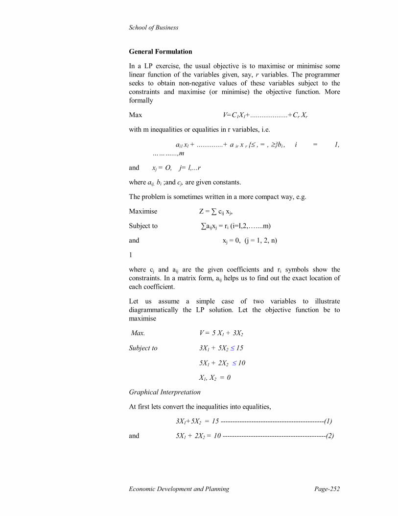
Graphical Interpretation
At first lets convert the inequalities into equalities,
3X1+5X2 = 15 --------------------------------------------(1)
and 5X1 + 2X2 = 10 --------------------------------------------(2)

Bangladesh Open University
Unit-5 Page-253
We get lines AB for equation (1) and CD for (2) in the figure. Here note that any point on or below the line AB satisfies the inequality 3X1 + 5X2 = 15; similarly any point on or below CD satisfies the inequality, 5 XI + 2X2 = 10. No point above AB (or CD) which satisfies the above inequalities. The points which will satisfy both the non-negativity constraints are given by the area OAKD. This area is then regarded as a feasible region. Any point such as P is regarded as feasible because of X1 and X2 at point P does not violate the constraints. Note that a feasible solution could lie at a point like O (at the origin). But such a feasible solution should imply that no production of (XI and X2 would take place. In order to obtain the optimum feasible solution it is necessary to find out the point at which the iso-profit curve is tangent to any point lying on AKD. Any iso-profit line such as V1 which lies inside the area OAKD does not yield the optimum profit because profit could always be increased by moving further away to a higher iso-profit line like V2 which just touches the area AKD at K. Similarly, the iso-profit line V1, although indicating higher profit, is not attainable. Thus, the optimum profit is given at the point K where OM of X 1 and ON of X2 will be produced. Thus at K the objective function V = 5X1 + 3X2 is at a maximum. It is necessary to point out here that given the above profit equations, iso-profit lines are straight lines. Since constant returns to scale operate, the further we move away from the origin along the iso-profit line, the greater is the level of profit. The iso-profit lines, i.e, V1, V2 etc. are parallel to one another.
To obtain the optimal values of XI and X2, it is necessary to solve the two equations for lines AB and CD at K.
X1 B D O M
N
A
C 5X1 + 2X2 = 10
K
P
V1
V2

School of Business
Economic Development and Planning Page-254
So we have:
3X1 + 5X2 = 15
5X1 + 2X2 = 10
Solving for X1 we have X1 = 1.053, for X2 = 2.368. The maximum profit now is V = 12.37.
The above example of solving the LP problem is highly simplified. In reality, it is generally found that an optimum solution has to be found subject to some inequalities in the constraints. These inequalities are usually converted into equalities by adding extra or 'slack' variables for solving the equations. Optimum solutions are then derived by using the 'simplex' method. In the simplex method, the optimum solution is reached via an iterative procedure. According to the rules of LP, any corner solution such as O, A, K, D, in the figure is a basic solution. In the simplex method, starting from any basic solution (e:g. O), we move to the adjacent corner solution (e.g.. either A or K) to improve upon the value of the objective function until the optimum reached optimal.
Limitations
While it is apparent that techniques of linear programming have important uses, the technique is constrained by several limitations. Some of them are:
1. Linearity handicap: The basic shortcoming of the technique arises from the linearity condition involved in it. The limitations arising out of this can be spelt out in terms of two central properties of linearity; additivity and mutiplicative relations. These two properties can hold in some cases, but not necessarily in all.
2. Useful in reality and approximate reality: The above criticism is no doubt valid because in real world situation is largely non-linear. It is not easy to find by established means the non-linear equations which express how prices and costs vary with output. Even if one had the equation, they would be difficult to solve unless they were unrealistically simple.
3. Statistical difficulties: The statistical difficulty arises more seriously in respect of industrial technology, in particular of industries, which do not exist or which are not yet established.

Bangladesh Open University
Unit-5 Page-255
Questions for review
1 Linear model is applicable for a. Only one variable b. Two variables c. More than two variables d. None of the above
2. Why linear model is unrealistic?
A. In real world situation is mostly non-linear. B. In real world situation is mostly linear. C. None of the above D. Both A and B
Answer 1.B, 2.A, Short questions
1. What are the usages of Linear Programming? 2. What is feasible region? 3. What is "simplex method"? 4. Why is it necessary to use simplex method?
Essay Type Questions 1. “The linear programming provides systematic examination of a
number of feasible alternatives,” – explain using diagrams and equations.
2. Assume two commodities x and y. At their prices each x earns a profit of Tk. 1040 and each y earns a profit of Taka 900. The x commodity requires 80 hours for processing and 48 hours for finishing. The y commodity requires 50 hours of processing and 60 hours for finishing. The firm has 800 hours of labour and 720 hours of labour for processing and finishing respectively in a week. How many of each commodity x and y firm should produce?
Further Readings: 1. Lal A N K, Economics of Development and Planing, Vikas
Publishing House Pvt. Ltd., 1997 2. Arrow, K.J., L. Hurwicz, and H. Uzawa, eds., Studies in Linear and
non Linear Programming, Standford, Calli: Standford University Press, 1958.
3. Hadley, G., Linear Programming, Mass.: Addison-Wesley, 1962. 4. Dervis, K., Melo, J. and Robinson, S., General Equilibrium Model
for Development Policy, The World Bank, Washington D.C., 1982. 5. Allen, R. G. D., Mathematical Economics, London, Macmillan,
1960. 6. Arrow,K., S. Karlin, and P. Suppes,eds., Mathematical Methods in
Social Sciences, Standford, Califf., Standford University Press, 1960.

School of Business
Economic Development and Planning Page-256
Lesson 3: Social Accounting Matrix (Sam) Objectives: Social accounting matrix is designed to serve mainly two purposes: the first is concerned with the organisation of information (i.e. information about economic and social structure of a country in a particular year) and the second is related to provide the statistical basis for the creation of a plausible model.
After studying this lesson, you will be able to:
Understand the framework of the SAM
Use SAM Introduction The Social accounting matrix (SAM) is double account book keeping, it deals with the series of accounts of which incomings and outgoings must balance; that means what is incoming into one account must be outgoing from another account. In this sense SAM embodies the information normally included in the national account. Here double entries are gained by only a single entry in a matrix. Each consists of one row and one column. The following example would be very useful to us to understand the operation of SAM. Let us assume that Robinson is engaged in only one production activity, say the picking of coconuts. In some given period, he picks 1,000 coconuts. This represents at the same time the level of production, the level of his income, and the level of his demand for products (sometimes called "wants"). All three are equal, as they must be in such an economy. The SAM for Robinson Crusoe
Expenditure Total
1 2 3 4 5 6
R E C E I P T S
1 2 3 4 5
Income Demand ………. Production ………
1000 1000
1000 1000 1000 1000
6 Total 1000 1000 1000

Bangladesh Open University
Unit-5 Page-257
The structure of this economy is set out in the table, in which two columns and rows have been left, blank because they are not being used for the time being. The final column and row around the border show the total of each row or column. Within the border there are three entries, each of them equal to 1,000. These constitute the SAM for Robinson Crusoe. In a SAM the rows represent incomings and the columns outgoings. For example, row 1,which is labeled "income," receives 1,000 from column 4, labeled "production." In other words, Robinson Crusoe's income derives from production and equals 1,000. Now, turning to column 1, we see the corresponding entry 1,000, which represents the outgoings of income in row 2, which is labeled "demand." Column/row 1, in effect, describes Robinson Crusoe's role as an income earner. In column/row 2, we look at him as a consumer. His demand arising from income in row 2 is balanced by what he spends on production in column 2 (row 4). The third leg of this process is in row 4 and column 4, where he turns up a third time as producer: his demand for production is 1,000 and income arising from production is also 1,000. These various identities could be set out in the form of double entry accounts, but, although not so apparent yet, the matrix is more economical since it requires one entry for each item, whereas conventional accounts require two. It will be noted that there is a circular process. If one put the three entries in the table in co-ordinate form with the row first and column second, they would appear like this: (1, 4); ( 4, 2 ); and ( 2, 1 ). Thus, the matrix illustrates the circular process of demand leading to production leading to income, which in turn leads back to demand. Of course, this rather complicated way of setting out the trivial structure of the Robinson Crusoe economy might well be considered much ado about nothing. We present it this way, however, because it is so self-evident and can serve as an introduction to the more complex relationships in an actual economy. In real life, Robinson Crusoe as a member of a society may, indeed, fill all three roles-as income earner, consumer, and producer-but he would do so as a member of different sorts of units or subdivisions, according to his function. In the accounts for a whole society, income may be subdivided into many different categories, among which income to labour and income to capital are only the first tier. That income accrues to a variety of domestic institutions, which are the source of demand: households with different characteristics, firms, and government (central or local). The outgoings or expenditures of these institutions are spread over a variety of products, as indeed Robinson Crusoe's must have been; production thus can be divided into as many sectors or subsectors as is desirable or practical.

School of Business
Economic Development and Planning Page-258
The uses of SAM The uses of SAM fall into two categories: those in which the whole corpus of information in the SAM is used and those in which only a part is used. Of course, in the latter case, it is not necessary to have the complete SAM. But the construction of the complete articulated SAM means that one has at one's disposal a multipurpose tool and does not have to construct separate subsets of accounts for each purpose. One of the principal ways in which the whole corpus of information in a SAM can be brought to bear is through multiplier analysis, which shows how changes in one or more elements of a SAM generate changes elsewhere in the matrix. Here we will only consider a simple example to illustrate the approach. The starting point is to assume a simple economy and a high1y aggregated SAM which has accounts only for the private sector, government production, the rest of the world, and a combined capital account. To keep things even simpler, it is assumed that only the private sector buys goods from the rest of the world. Corresponding to this simple economy, we assume we have a SAM for some base period, and we ask the question, "What would happen if demands on production activities were increased by increasing government expenditure (by an amount i2), investment (by an amount i3), and exports (by an amount i6)?" Without loss of generality we can put the sum of the i's equal to one. The first part of the answer to this question is that whatever the processes of consequential changes might be, the end result will be a new SAM for our simple economy. Moreover, those elements of the initial SAM that are zero by definition will remain zero. Because our model assumes that only the private sector buys goods from abroad, the purchases of such goods by the government, for example, will remain zero. Given the accounting rules and model assumptions, the difference between the new SAM and the original one will imply an incremental SAM in which many cells have zero entries. This incremental SAM is shown in table. At this stage we know the items i2, i3, and is, because these are the changes that we have exogenously postulated. We also know that the blank entries in the table are zeros, because these follow from our model and accounting conventions. The question then is, "What can be said about the nonzero entries apart from i2, i3, and i5?” Not much can be said about these nonzero entries without making further assumptions about what will happen, for example, to prices, monetary policy, and how people choose to spend any extra income. We will assume, for simplicity, that private sector income goes up by an amount M, and then explore what the incremental SAM in table can say about the relationships between M and the i's.

Bangladesh Open University
Unit-5 Page-259
Table: Multiplier effects in the form of SAM
Expenditure Total
Receipts 1 2 3 4 5 6
1
Private Sector M M
2 Government Mp2 Mp2
3 Capital Account Mp3 Mp2-i2 i3
4 Production Mp4 i2 i3 Mp5-i5 M
5 Rest of the World Mp5 i5 Mp5
6 Total M Mp2 i3 M Mp5
Note:M(1-p4) = Σ p = Σi
p2 = marginal propensity to tax
p3 = marginal propensity to save
p4 = marginal propensity to consume (domestic)
p5 = marginal propensity to import
M = Multiplier
i2 = Impulse from increased government expenditure
i3 = Impulse from increased investment
i5 = Impulse from increased exports
Because in this simple model the private sector gets all its income from production activities and because these activities pay all value added to the private sector, row 1 and column 4 of the incremental SAM are very simple and contain zeros apart from the entry in row 1, column 4, which is M.
The increase in private income (row 1) must match the increase in private expenditures in
column 1. The latter must now be spread over the different components of private expenditures. This spread is assumed to take place in the proportions P2, P3, P4, and P5, which can be referred to as the marginal expenditure propensities of the private sector. Because all the extra income M must be spent or saved, the accounting balance for row/column 1 implies that
p2 + p3 + p4 + p5 = 1.
School of Business
Economic Development and Planning Page-260
We might also be prepared to assume that these propensities are constant. But if we do, then this is clearly a behavioural assumption, not an accounting rule.
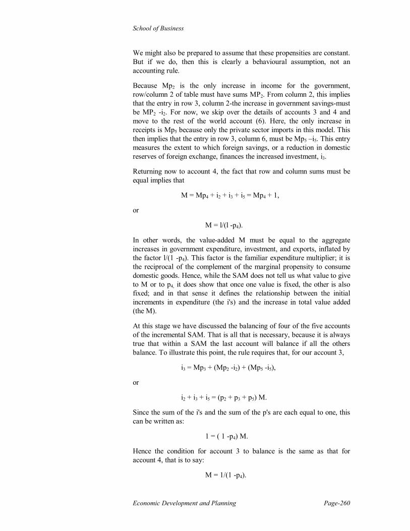
Because Mp2 is the only increase in income for the government, row/column 2 of table must have sums MP2. From column 2, this implies that the entry in row 3, column 2-the increase in government savings-must be MP2 -i2. For now, we skip over the details of accounts 3 and 4 and move to the rest of the world account (6). Here, the only increase in receipts is Mp5 because only the private sector imports in this model. This then implies that the entry in row 3, column 6, must be Mp5 –i5. This entry measures the extent to which foreign savings, or a reduction in domestic reserves of foreign exchange, finances the increased investment, i3.
Returning now to account 4, the fact that row and column sums must be equal implies that
M = Mp4 + i2 + i3 + i5 = Mp4 + 1,
or
M = l/(l -p4).
In other words, the value-added M must be equal to the aggregate increases in government expenditure, investment, and exports, inflated by the factor l/(1 -p4). This factor is the familiar expenditure multiplier; it is the reciprocal of the complement of the marginal propensity to consume domestic goods. Hence, while the SAM does not tell us what value to give to M or to p4, it does show that once one value is fixed, the other is also fixed; and in that sense it defines the relationship between the initial increments in expenditure (the i's) and the increase in total value added (the M).
At this stage we have discussed the balancing of four of the five accounts of the incremental SAM. That is all that is necessary, because it is always true that within a SAM the last account will balance if all the others balance. To illustrate this point, the rule requires that, for our account 3,
i3 = Mp3 + (Mp2 -i2) + (Mp5 -i5),
or
i2 + i3 + i5 = (p2 + p3 + p5) M.
Since the sum of the i's and the sum of the p's are each equal to one, this can be written as:
1 = ( 1 -p4) M.
Hence the condition for account 3 to balance is the same as that for account 4, that is to say:
M = 1/(1 -p4).

Bangladesh Open University
Unit-5 Page-261
This result simply repeats that obtained previously. If all but one account are balanced, then all accounts are balanced, and the story of the incremental SAM shown as table is thus completed.
The application of multiplier analysis with a complete SAM is little different in principle, though it is far more complex. It takes into account all the interactions with1n each step of the process of linkages among incomes, expenditures, and production. The linkages could include, for example, the effects on other industries of expansion with1n a particular industry. There is, however, no longer a single multiplier, but an entire matrix of multipliers, which potentially shows the effect of expansion in one cell of the original SAM on any other cell. How these effects are to be interpreted must always be approached with care because the effect of one variable on another ultimately depends on economic behaviour and not just on accounting constraints. However, the approach has some value in distinguishing accounts or subaccounts that are likely to be affected from those that are likely to be bypassed. This distinction may well have importance in considering the effect of exogenous changes on the distribution of income. The analysis may also serve to identify the important elements that result in changes in government accounts or in the balance of payments.

School of Business
Economic Development and Planning Page-262
Review Questions 1. What is SAM? 2. Construct SAM of Robinson Crusoe economy? 3. Analyse multiplier effect in the form of SAM?
Further Readings:
1. Pyatt, G., and J. Round (1979a), ‘Social Accounting Matrices for Development Planning’, The Review of Income and Wealth, Series 23, no.4, pp-339-64.
2. Pyatt, G., and J. Round (1979b), ‘Accounting and Fixed Price Multipliers in a Social Accounting Framework,’ Economic Journal, Vol.89,pp-850-73.
Bangladesh Open University
Unit-5 Page-263
Lesson 4: Computable General Equilibrium Model2 Objectives: Computable general equilibrium (CGE) models combine features from the different types of planning techniques that are discussed in the preceding lessons. They are based on socio-economic structure of SAM with its multisectoral multiclass disaggregation, incorporating initial inputs from input-output table. The CGE models have been used for policy analysis to comprehend shocks, changes in economic polices, etc.
After studying this lesson, you will be able to:
Discuss the basic structure and equations of Computable General Equilibrium Models.
Understand the construction of the CGE Model
Discuss the solution strategies of CGE Model Introduction A CGE can be described by specifying the agents and their behaviour, the rules that bring the different markets in equilibrium and the macroeconomic characteristics. Structure of CGE Models In a CGE producers are profit maximisers and chose their levels of production and purchases on the basis of prices. Domestic products and imports are imperfect substitute and the composition of domestic supply depends on their relative prices. Household maximise their utility and choose levels of consumption based on income and prices. In a CGE all the accounts are endogenous and thus must be in equilibrium. Producers sell their total production, factors distribute their income, firms and households spend their income and investment is determined by available savings. Excepting the government which is balanced by letting its savings, or deficit if negative residually computed, others occur through the markets. The standard rule is one of price flexibility and endogenous determination of the equilibrium process. There are four macroeconomic components in a CGE. These are: the balance of payment, the savings-investment equilibrium, the government budget and aggregate supply of primary factors of production. The balance of payment is constrained to an externally defined level of deficit. Except in the structuralist models, total investment is assumed to total savings. The budgetary consequences of all policies are accounted for in CGE. In most models capital is considered fixed and fully utilised. 2Based on Dervis K., De Melo J., Robinson S. General Equilibrium Model for Development Policy. World Bank. Washington, D.C. 1982.

School of Business
Economic Development and Planning Page-264
The behavioural assumptions of a CGE model are usually that agents respond to relative prices rather than to the absolute level of any price. All demand and supply functions are homogenous of degree zero in all prices. It is standard procedure to set one price or a price index constant.
Construction of Computable General Equilibrium Model3
The production technology for primary factors is described by a neoclassical production function that allows smooth substitution among factor inputs. The degree of substitutability is governed by the elasticities of substitution (in this case constant elasticity of substitution production function). According to a two-level production function where gross outputs are related to input the equation will be Xi = fi(At
/, Kt/,Li
a,Via)--------------------------------------------(1)
where Xi = sectoral output
At/ = a shift parameter that will dynamically reflect
disembodied technical progress.
Kt/ = the stock of the aggregate capital goods assumed to be
fixed by sectors.
Lia = an aggregation labour inputs.
Via = an aggregation index of intermediate inputs.
Given both the shares among different intermediate inputs in a sector and the ratios of intermediate inputs are fixed, the demands for intermediate inputs will be
Vij = aij Xj --------------------------------------(2)
where aij are the input-output coefficients. Now for getting total intermediate demand by sector of origin it can be written Vi = Vij = aijXj ---------------------------------------(3) j j The sectoral labour input is assumed to be an aggregation of labour of different skill categories. The function will be represented by the equation ( with m types of goods)
Lia = Lia(Li1……………….Lim)-----------------(4)
3 K. J. Arrow, H. B. Chenery, B. S. Minhas, and R. M. Solow, ‘Capital-Labour Substitution and Economic Efficiency,’ Review of Economic and Statistics, August 1961,pp- 225-250.

Bangladesh Open University
Unit-5 Page-265
This equation is given by the CES function with a single elasticity of substitution among all labour categories. The specification of the production set of the economy is incomplete without a set of factor availability constraints; writing in the form of excess demand functions for labours
Lis - Ls/ = 0-------------------------------(5)
i where Ls
/ denotes the fixed supplies of the various categories of labour. Each sector in the economy is treated as made up of many similar firms maximising profits; the assumption of perfect competition in product markets amounts to assuming that firms take commodity prices as given. Under this circumstances, one can treat each sector as one large price taking firm. The aggregate sectoral profit functions are given by
i = Pi(1-tdi)Xi - PjaijXi- Ws Lis----------------(6) j j
Where Ws is the wage of labour of type s and tdi is the indirect tax rate. 4 The profit equation can be rewritten as
i = PNiX - Ws Lis j
where n PNi = Pi(1-tdi) - Pjaij-------------------------(7)
j=1 is the or value-added coefficient, this time net of indirect taxes. Labour demands are given by PNidXi/dLi
a dLia /dLis= Wi-------------------------------(8)
This equations give the demand functions by sectors for labour and may be written as Lis = Fis (W1…………….Wm,,PN1, Kt
/)-------------------------(9) The equations for the factor markets which essentially underlie the aggregate supply or production transformation set considered is collected together in the following table.
4 The primary concern in this simple model is not with policy formulation, the inclusion of a government sector leads to naturally to the inclusion of indirect tax and direct tax in the system.

School of Business
Economic Development and Planning Page-266
Tablie1: Factor market and product supply equations: No of
equations
Production function: Xis = f(k/
1, Lia,V1,……..,Vm)
Intermediate goods demand Vij = aij Xj Vi = Vij j Labour aggregation Lia = Lia(Li1, Li2 ……. Lim) Net prices PNi = Pi - Pjaji -tdi Pi j Labour demand equations PNidXi/dLi
a dLia /dLis= Wi
Aggregate labour demands Ld
s = Lu Aggregate labour supply Li
s = L/ Excess demand for labour equations Li
s = Lss =0
Total: 4n+3m+n . m+n. n
n n.n n n n.m m m m
1 2 3 4 5 6 7 8 9
Endogeneous variable Xi
s Sectoral Production Vij Intermediate goods demand Vi Aggregate intermediate goods demand Li
a Aggregate labour by sector PNi Net prices Lis Labour demand by sector and prices Ls
d Aggregate labour demand by type Ls
s Aggregate labour supply by type Ws Wage of labour by type Total:4n + 3m+n.m+n.n
number n n.n n n n n.m m m m
Tablie2: Product market equations: No of equations Household capitalist and government income: Yi = Wi,Lis(1-ti) Yi = [PMiXi - Lis](1-ti) Yi = {ti/(1-ti)}Ys + {ti/(1-ti)}Ys +tdiPiXi Total Savings TS = SsYs +SkYk +Sg Yg
Consumer Demand
m one one one
10 11 12 13

Bangladesh Open University
Unit-5 Page-267
Cid = Cis
d + Cikd + Cig
d
Investment Demand Ui =sij Pj Ki =Hi
/ [TS/Ui] Zi =sijKi Aggregate Excess Demand Xd
i =Cid+Zi+Vi
Xdi- Xs
i=0 Price Normlisation Pii=P/
Total: 4n+3m+n . m+n. n
n n n n n n one
14 15 16 17 18 19 20
Endogeneous variable Ys Labour Income by type Yk Capital Income by type Yg Government revenue TS Total Saving Ci
d Aggregate consumption demand Cis
d Consumer Demands by labour house holds Cik
d Consumer demands by capitalist Cig
d Government Consumption
Ui Capiral goods price Ki Real Investment Zi Investment goods demand by sector of origin Xd
i Aggregate demand by sector P/ Prices Total:4n + 3m+n.m+n.n
number m one one n.m n n n n n n n n n
The endogenous variables in these equations describe all the flows in the first column of the social accounting matrix. In real life employment, intermediate demand, and product supply are covered here and in terms of monetary flows, they give payments for intermediate goods, labour, capital, and indirect taxes. Table 2 shows the equations for the product markets in the model economy. The endogenous variables describe the flows in the last four columns of the social accounting matrix. They give the distribution of factor income to "institutions" {households and government); its allocation among taxes, consumption and saving; and finally the resulting demand for products. The presentation in Tables 1 and 2 emphasises the market-clearing role of wages and prices in the core model. For any given set of product prices Pi there are as many equations in Table 1 as there are endogenous variables. The heart of the problem is to find a set of average wages such that, given

School of Business
Economic Development and Planning Page-268
the labour demands from Eq. (6), there is zero excess demand in the markets for labour of different categories. The solution of the excess demand equations for labour for different sets of product prices defines the summary numerical supply function given in Eq. (11). In Table 2 the product market equations can, by simple substitution, be reduced to the set of excess demand equations. Note that the number of equations is one greater than the number of variables. As we have discussed, the equations are not independent, so' that the n excess demand equations can determine only n - 1 relative prices. The price normalisation equation (20) is required to set the absolute price level. The product market equations include the flow of funds among the various institutions in the economy. They thus include the flows that are the focus of demand-driven macro models. We are focusing on issues of sectoral structure, resource allocation, and trade, and so are not attempting to determine endogenously variables such as the price level. However in any CGE model, the flow of funds accounts must specify the entire circular flow in the system - There are no leakages. The treatment of investment In the equations presented in Table 2, the sectoral share parameters for investment (Hi
/) are simply assumed to be fixed. The level of total, investment, however, is determined endogenously. In the capital account row in the SAM, total savings (and hence investment) are determined; by applying exogenous savings rates to the income of each institution in the economy. Total investment is thus determined by savings behaviour and is thus also a function of the distribution of income among the different households and the government (assuming that their savings rates differ). This model of total savings and investment is very classical in spirit, except that we have added government to the usual capitalist and labour classes. There is no shortage of theories of investment in economics -the problem is more that there is no widespread agreement on which theories are best. In a planning model such as CGE model; a number of different choices seems reasonable. Solution strategies There are several ways to solve CGE models but it is useful to distinguish between a solution strategy and a solution algorithm. A solution strategy refers to the way in which the equations of the model are substituted and rearranged so as to reduce the solution problem. A solution algorithm refers to the actual numerical algorithm used to solve the reduced set of equations. In devising a solution strategy for CGE models, it is important to take advantage of our knowledge of the economic properties of the system of equations.

Bangladesh Open University
Unit-5 Page-269
In choosing a solution strategy, two criteria are most important. First, how hard is it to solve the reduced equations numerically? Second, how hard is it to reduce the model equations to the chosen set, especially when, as is often the case, one wants to be able to experiment with a variety of analytic formulations ?Reducing a CG E model to sets of market excess demand equations is usually a straightforward procedure requiring, with one exception, simply the evaluation of the equations of the model in order. The only place where numerical techniques may have to be used is in the derivation of labour demands by firms given wages -the marginal revenue product equations. All solution algorithms will follow the same general procedure. They will all start with some initial set of wages and prices (which .satisfy the normalisation rule), calculate the excess demands in both factor and product markets, and then revise wages and prices iteratively based on calculated excess demands. The iterations stop when equilibrium is reached; that is, a set of wages and prices is found such that all excess demands are sufficiently close to zero. Different algorithms use quite different techniques for revising wages and prices given the excess demands from the last iteration, and there are a variety of such algorithms from which to choose.

School of Business
Economic Development and Planning Page-270
Review Questions 1. Describe structure of a CGE Model. 2. How is the investment treated in CGE model? 3. Discuss solution strategies of a CGE model.
Further Readings 1. Arrow, K. and F. Hahn(1971), General Competitive Analysis, San
Fransisco Holden-Day. 2. Arrow, K.J., L. Hurwicz, and H. Uzawa, eds., Studies in Linear and
non Linear Programming, Standford, Calli: Standford University Press, 1958.
3. Dervis, K., Melo, J. and Robinson, S., General Equilibrium Model for Development Policy, The World Bank, Washington D.C., 1982.
4. Arrow,K., S. Karlin, and P. Suppes,eds., Mathematical Methods in Social Sciences, Standford, Califf., Standford University Press, 1960.

Bangladesh Open University
Unit-5 Page-271
Lesson 5: Cost-Benefit Analysis (CBA) Objectives:
The choice of project and allocation of resources has been dominated by social cost benefit analysis. The technique, in the post 1970s era, has been recommended for the appraisal of publicly financed investment projects in order to achieve allocative efficiency.
After studying this lesson, you will be able to:
Explain the meaning of social cost-benefit analysis. Explain how the cost benefit analysis of a project to society may
differ from the cost-benefits to the private entrepreneur. Describe the decision rules in CBA. Explain the reason for using CBA in LDCs. Introduction How should a project’s social benefits and costs be measured? What common units of account should the benefits and costs be expressed in, given a society’s objectives especially in circumstances when it has trading opportunities with the rest of the world? There are several ways of undertaking such questions. Benefits and costs may be measured at domestic market prices using consumption as numeraire, with adjustments made for divergence between market prices and social values, and making domestic and foreign resources comparable using a shadow price of foreign exchange. This is sometimes referred to as the UNIDO approach [Dasgupta, Marglin and Sen(1972)] Benefits and costs may measured at world prices to reflect the true opportunity costs of outputs and inputs using public saving measured in foreign exchange as numerair.(i.e. Converting everything into its foreign exchange equivalent). This referred to as the Little-Mirrlees approach [Little and Mirrlees (1969) and (1974)] Basic Principles of CBA Here the objective is to choose the project that high yields high positive Net Social Benefit (NSB) where the NSB is defined as NSB = Benefits (willingness to pay) -Costs (compensation needed).

School of Business
Economic Development and Planning Page-272
All benefits and costs are expressed in monetary units. The willingness to pay is given by the area under the demand curve, but the actual total price paid is given by the price times the quantity .In other words, the amount of consumer surplus reflects the size of gains. So in the figure though the consumers are willing to pay ODSM for OM quantity, they actually pay OPSM and hence the area DPS measures consumers’ surplus. Now lets suppose that a cost saving device is used in project, prices fall to OP1 from OP, and an increase in the goods provided is shown by MM1. Here the total willingness to pay is given by ODS1M1 which is greater than ODSM by MSS1M1 out of which MM1S1E accounts for actua1 payments and as such, the change in consumer surplus is given by the shaded area ESS1. This is equivalent to the NSB for the society. Many problems lie with the estimation of this social benefit. For example, the demand curve is assumed to be linear, marginal utility of income is supposed to remain fixed; utility is supposed to be measurable cardinally, prices of all other goods are expected to remain unchanged; there are some intangibles which cannot be measured. Hicks tried to tack1e some of these problems by allowing changes in the marginal utility of income and by using the indifference curve analysis. Also, Kaldor and Hicks pointed out that to increase social welfare, it is only necessary to show that the gainers should be able to compensate the losers and still remain gainers. Moreover, as Scitovsky points out, if the gainers can compensate the losers in accepting a change and the losers can bribe the gainers back to the ‘status quo’ then a clear contradiction emerges as there is no way to tell whether social welfare has increased or discreased.
Rate of Discount
NPV
O
A
Quality Demanded
D
P
P1
S
S1
O M M1
E

Bangladesh Open University
Unit-5 Page-273
The decision rules in CBA
To take decisions regarding project choice, the project planner confronts the following sets of problems:
(a) the problem of identification of the benefits and costs;
(b) the problem of valuation of these benefits and costs at prices which would be relevant to society;
(c) the problem of choosing an appropriate rate of discount for evaluating such benefits and costs;
(a) the problem of identifying the actual constraints;
(e) the problem of uncertainty.
At this point the planner tries to find out the Net Present Value (NPV) discounted by a certain rate of discount and if the NPV > 0, then the project should be accepted. If the projects are mutually exclusive, then the one which yields the highest NPV should be accepted. Note that NPV means prescient discounted value of benefits less present discounted value of costs. More formally, if the net benefits arc given by P1, P2,
NPV = Pt/ (1 + i t) where i = rate of discount. This could be a social rate of discount or opportunity cost of capital. In practice. the choice is rather difficult. It is obvious that the higher rate of discount the lower will be the NPV (see Figure), and at a certain rate of discount, the NPV = 0. Such a rate is called internal rare of return (IRI) or OA in Fig.
More formally,
[Pt / (1+ µ )t] = 0 where A = internal rate of return. If µ > i then the project should be accepted if not, the project should be rejected. Reasons for undertaking CBA in LDCs
Several reasons are given for undertaking CBA for the LDCs to make a realistic estimated of the net social benefits (NSB) 1. Inflation in many LDCs, emanating chiefly from the supply inelasticities, alters the relative prices and government's intervention in the form of price controls results in the distortion of NSB. 2. In most LDCs, exchange rates of the, domestic currencies are kept artificially high. This again leads to an excess demand for foreign exchange and when the government imposes import restrictions, market
School of Business
Economic Development and Planning Page-274
prices of goods exceed their world price and such market prices tend to overestimate the NSB within the country. 3. Given the imperfections of the labour market in the LDCs, different modes of production (e.g. use of family labour rather than wage labour and the absence of a unique relationship between marginal productivity of labour and wages) and the presence of large-scale unemployment, it is argued that wages paid to labourers in LDCs tend to overestimate their true social opportunity costs. Hence a shadow wage rate should be calculated to work out the true cost of labour to society. 4.Given the imperfections of the capital market in most, the interest rate is kept artificially low, particularly when capital is very scarce in supply. Here again, a shadow rate of interest should be calculated to remove the underestimation of the cost of capital to sociery. 5. Since large projects are likely to yield significant secondary benefits to the economy, it is not enough to count only the primary benefits of a project. 6. Since many LDCs have decided to industrialise their economies behind protectionist walls by using tariffs, quotas, exchange controls, etc., market prices within the economy would fail to reflect the NSB. 7. Saving deficiency and public income Given the dearth of savings in LDCs, the government can value an extra unit of saving more than the extra unit of consumption and impose appropriate taxes (which of course imposes some costs) to raise, such savings. It is assumed that money at the disposal of the government of any country is worth more than private consumption because while money in the hands of the government could be invested to produce future consumption, it would be wasteful if left in the hands of private individuals who have very high propensity to consume. 8. The problem of inequalities in the distribution of income and wealth is very much present in the LDCs. Such a problem would be lessened if public savings could substitute for private savings by the rich in LDCs. 9. It is argued that whenever externalities are present say, in the presence of diminishing costs in certain industries with a large investment project), such externalities should be fully taken into account in the project appraisal for the LDCs. The Equivalence of the Little-Mirrlees Formulation of the Shadow Wage and the Unido Approach In the Unido approach, the optimal shadow wage is given by

Bangladesh Open University
Unit-5 Page-275
W* = PA + s* ( PINV -1) W ------------------------------------(1) Where s* is the capitalists propensity to save,
W* is the wage PINV measures the price of investment in terms of consumption.
Assuming that the propensity to save of capitalists is unity (s*= 1) and all wages are consumed, equation (1) may be written as W* = PA + ( PINV -1)C ------------------------------------(2) Where ( PINV -1)C represents the present value of aggregate consumption lost (assuming PINV 1) because of the increased consumption of workers which reduces savings for future consumption. Now for the two approaches to give the equivalent cash flows, which ever numeraire is taken, PINV must equal So, so that equation (2) may be written as: W* = PA + (S0 -1)C ------------------------------------(3) Now the little Mirrlees formulation of the shadow wages is: W* = PA + (1 -1/S0)(C-m) ------------------------------------(4) Which, on the assumption that PA= m , may be written as W* = PA /S0+ (1 -1/S0)C ------------------------------------(5) Comparing equation (4) with the UNIDO equation (3) it can be see that the UNIDO formula is S0 tomes the Little-Mirrlees formula because the UNIDO numeraire is 1/S0 times as valuable as the Little-Mirrlees numeraire. A Comparison of Little-Mirrlees and UNIDO Approaches Little-Mirrless
Y0 Y1 Y2
UNIDO Y0 Y1 Y2
Cost of investment(k) 1.Foreign component 2.Local Component= 1000 convesion factor of 0.8
$1000 $800
1.Foreign cost converted into taka at shadow exchange rate of 1.25 2.Local component
Tk.1250 Tk.1000

School of Business
Economic Development and Planning Page-276
Input Cost(C) 1.traded inputs 2.Non-trade inputs= 1000 convesion factor of 0.8
$1000 $1000 $800 $800
1.Traded inputs converted into taka at shadow exchange rate of 1.25 2.Non-traded inputs
Tk.1250 Tk.1250 Tk.1000 Tk.1000
Benefit Flow(v)
$3000 $3000
Benefit flows in Taka
Tk.3750 Tk.3750
Net Benefit $1800 $1200 $1200
Net Benefit in Taka
Tk.2250 Tk.1500 Tk.1500
A Numerical Example: Assume that the world price are measured in dollars and domestic price are measured in taka(Tk.); that the shadow exchange rate is 1.25 taka per dollar; that the shadow price of foreign exchange (PF)=1.25 and the standard factor for converting non-traded goods prices into world prices is0.8 . Assume further that : 1. All output is exported with an annual value of $3000 2. The cost of investment has a foreign component of $1000 and a local
component of Tk. 10000. 3. There are traded inputs of $1000 and nontraded inputs of Tk.1000. 4. The accounting rate of interest is equal to the consumption rate of
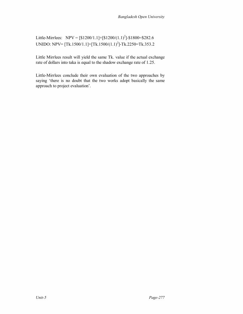
interest. We can apply our net present value formula using two approaches. Remember that using Little-Mirrlees approach we must convert all the prices of nontraded goods into world prices using the standard conversation factor of 0.8, and using UNIDO approach we must convert all the values at world prices($) into domestic prices using the shadow exchange rate of 1.25 We will do the analysis for three periods only (see table). We see that the results of using the Little-Mirrlees approach and the UNIDO approach will differ only to the extent that the shadow exchange rate is different from the actual exchange rate. To obtain the net present value, the net benefit stream in years 1 and 2 must be discounted by the appropriate discount factors which we assume here to be the same using both approaches. Assuming the discount rate of 10 percent we have:
Bangladesh Open University
Unit-5 Page-277
Little-Mirrlees: NPV = [$1200/1.1]+[$1200/(1.1)2]-$1800=$282.6 UNIDO: NPV= [Tk.1500/1.1]+[Tk.1500/(1.1)2]-Tk.2250=Tk.353.2 Little Mirrlees result will yield the same Tk. value if the actual exchange rate of dollars into taka is equal to the shadow exchange rate of 1.25. Little-Mirrlees conclude their own evaluation of the two approaches by saying ‘there is no doubt that the two works adopt basically the same approach to project evaluation’.

School of Business
Economic Development and Planning Page-278
Review Question 1. What is the meaning of social cosy-benefit analysis? 2. Explain hoe the cost benefit analysis of a project to society may differ
from the cost-benefits to the private entrepreneur? 3. What are the decision rules in CBA? 4. Why should CBA be used in LDCs? Further Readings
1. Janos Kornai, ‘Appraisal of Project Appraisal’, in Micheal J. Boskin (ed.), economics and Human Welfare: Essays in Honor of Tobor Scitovsky (New York, Academy press, 1979), pp. 91-96.
2. P. Thirlwall (1970) ‘The Shadow Wage when Consumption is Productive’, Bangladesh Development Studies, Oct-Dec.
3. M. Scott, J. Macarthur and D. Newbery (1976) Project Appraisal in Practice. (London: Heinemann)
4. G. B. Baldwin (1972) ‘A Layman’s Guide to Liltte-Mirrlees’, Finance and Development, vol. 9, no.1.
5. M. D. Little and J. Mirrlees (1974) Project Appraisal and Planning for Developing Countries, (London: Heinemann)
6. M. D. Little and J. Mirrlees (1969) Manual of Industrial Project Analysis in Developing Countries, vol.II Social Cost-Benefit Analysis (Paris: OECD)

Bangladesh Open University
Unit-5 Page-279
Lesson 6: Logical Framework Approach (LFA)5 Objectives:
The Logical Framework Approach (LFA) described in this section is based on the "Logical Framework " method, which is a way of structuring the main elements in a project, highlighting logical linkages between intended inputs, planned activities and expected results.
The purpose of the lesson is to: Explain the planning procedure which enables institutions to design a
programme or project. Describe the advantages of using LFA Explain stakeholder analysis. Explain the vertical and horizontal logics within project planning
matrix. Introduction The logical framework (or logframe) approach provides a set of designing tools that, when used creatively, can be used for planning, designing, implementing and evaluating projects. The purpose of LFA is to undertake participatory, objectives-oriented planning that spans the life of project or policy work to build stakeholder team commitment and capacity with a series of workshops. The first "Logical Framework" was developed for U.S.AID at the end of the 1960's, and has since been utilized by many of the larger donor organizations, both multilateral and bilateral. OECD's Development Assistance Committee is promoting use of the method among the member countries. The Nordic countries have also shown interest in the use of the "Logical Framework", and in Canada the approach is used not only in development aid but also in domestic public investment in general. Institutions in partner countries also use the LFA in their management of projects and programmes. The Advantages of LFA The advantages of using LFA are the following: It ensures that fundamental questions are asked and weaknesses are
analysed, in order to provide decision makers with better and more relevant information.
It guides systematic and logical analysis of the inter-related key elements which constitute a well-designed project.
5 Based on The Logical Framework Approach: Handbook for Objectives-oriented Planning, NORAD, January 1999 and materials used for UNDP/UNSO Capacity Building Workshop for Dryland Management

School of Business
Economic Development and Planning Page-280
It improves planning by highlighting linkages between project elements and external factors.
It provides a better basis for systematic monitoring and analysis of the effects of projects.
It facilitates common understanding and better communication between decision-makers, managers and other parties involved in the project.
Management and administration benefit from standardized procedures for collecting and assessing information.
The use of LFA and systematic monitoring ensures continuity of approach when original project staff are replaced.
As more institutions adopt the LFA concept it may facilitate communication between governments and donor agencies. Widespread use of the LFA format makes it easier to undertake both sectoral studies and comparative studies in general.
Steps in an LFA
There are 4 major steps in conducting an LFA, each with a set of activities to be carried out as outlined below:
Step - I. Situation Analysis
The LFA approach begins by analysing the existing situation and developing objectives for addressing real needs. A situation analysis has as its core task to find out the actual state of affairs with respect to an issue to be analysed; it is focussed by problems and an attempt to understand the system which determines the existence of
Situation Analysis (1) Stakeholder Analysis (2) Problem Analysis (3) Objective Analysis
Strategy Analysis
Project Planning Matrix
(1) Matrix (2) Assumptions (3) Objective Indicators (4) Verification
Implementation

Bangladesh Open University
Unit-5 Page-281
the problems. As problems are always connected to unfulfilled objectives, a situation analysis comprises of an Objectives’- as well as a Problems’-Analysis. And as it is always people’s problems and objectives which make up a situation, the analysis includes a Participants’-Analysis. The analysis phase is the most critical, yet most difficult, phase of the logframe approach. The analysis phase consists of three stages,
Analysis of stakeholders Analysis of problems Analysis of objectives.
The situation of the proposed project or programme needs to be analysed. Answers to the following questions are needed:
What are the general areas of concern, or themes, that the project will focus on?
What is the project aiming to achieve? At what spatial levels will the project focus, in terms of subject
(broad/macro to specific/micro) and or geography (local to global)?
What political, socio-economic, technological and biophysical environment will the project operate within?
Who are the major stakeholders? How will stakeholders be involved in the process of design,
implementation, monitoring, evaluation and reporting? Who is working on the issues already? What are they doing? What is the niche of the project? Who will implement the project? What is the intended duration of the project? What is the anticipated level of funding? Who will fund the project?
Stakeholder Analysis
Projects are influenced by many actors. Their different interests, potentials, deficiencies and other characteristics play a role in the process of designing and implementing a project. It has been a frequent experience in development that marginal groups were not sufficiently considered in the planning, and hence caused poor implementation. Thus it is usually necessary and expedient to analyse stakeholders in a project as part of the planning process.

School of Business
Economic Development and Planning Page-282
In using the LFA approach, the stakeholder analysis is an analysis of the problems, fears, interests, expectations, restrictions and potentials of all: - important groups - organisations and institutions - implementing agencies - other projects and - individuals who may have an influence on a situation/(intended) project or are themselves affected by it. Those analysed in detail should be limited to those who are perceived to: - be able to contribute to questions to be answered - be important with regard to decisions to be taken. They should constantly be referred to in developing the LFA. Key questions to ask in preparation for developing the logframe are: Who will be involved in the logframe development? Where will the development be conducted? Who will facilitate the development of the logframe? What background materials, papers and expertise may be needed? What materials and logistics are required? Analysis of Problems
The analysis phase usually begins with an analysis of problems. The problem analysis is undertaken by identifying the main problems and developing a 'problem tree' through an analysis of cause and effects. The guiding principle in the Analysis of Problems is: problem-focused analysis combined with a systems’ understanding Problem-focused analysis means: analyse only those issues which are identified to be problematic, be
guided by problem view narrowing the focus with respect to the scope of analysis and at the
same time digging deep into these problems and their causal factors. System’s understanding means: understand how the
system (in which the problem and its causing factors occur) operates
widening the view with respect to analysing the interlinkages and feed-back mechanisms
An example of brainstorming rules: (1) All ideas are accepted without argument (2) Aim for quantity rather than quality (3) No debate about whether ideas are accepted or not, only about whether the idea has already been listed. (4) No evaluation now (limit the discussion on the significance of the material and concentrate on getting full cross-section of ideas)

Bangladesh Open University
Unit-5 Page-283
between components of the system Brainstorming techniques can be used to identify the main problems. Before the brainstorming exercise commences it is important that the facilitator explain the process and the group agrees on some rules for brainstorming. Developing the Problem Tree The substantial and direct causes of the focal problem are placed parallel underneath it. The substantial and direct effects of the focal problem are placed parallel on the line above it. Causes and effects are further developed along the same principle to form the problem tree. If a workshop decides that the high number of accidents should be considered the focal problem. The following problem tree of substantive and direct causes and effects can be established
Objectives Analysis An objectives’-analysis in a wide sense is a procedure for systematically identifying,
The objectives-analysis and the problems-analysis influence each other: the more information one has about the problem situation, the more specifically one can formulate objectives; the kind and outline of the objectives analysed influence the perception of problems.

School of Business
Economic Development and Planning Page-284
categorising, specifying and - if required - balancing out objectives of all parties involved in a specific situation (for which those objectives apply). The problem tree is transformed into an objectives tree by restating the problems as objectives. The objectives tree can be viewed as the positive mirror image of the problem tree. It is usually necessary to reorder the position of objectives as you develop the tree. The objectives tree can also be considered as an 'ends - means' diagram. The top of the tree is the end that is desired and the lower levels are the means to achieving the end.
If the workshop decides to add "training of drivers" as a means to make drivers more responsible. Step – II: Strategy Analysis
A strategy analysis or analysis of alternatives is a systematic way of searching for and deciding on problem solutions. It follows the problems and objectives analysis and is a prerequisite to designing action strategies. Choices among different solutions to problems may concern
overall concepts, strategic
Alternative strategies can only be analysed as different means (the “how”: doing the thing right) to reach a pre-defined end (the “what”: doing the right thing). Analysing the strategies thus is not a once for all exercise, but it is a continuous task in project management.

Bangladesh Open University
Unit-5 Page-285
plans, objectives people, target groups, organisations, agencies methods, procedures, processes technologies, services, products, outputs measures, actions, materials, inputs
All alternative strategies considered must contribute to solving a problem, or in other words: they must be suitable steps towards the attainment of identified guiding objectives (relevance). Based on the situation analysis and the ordering sequence of the problem and objective trees, the strategy analysis involves clustering objectives and examines the feasibility of different interventions. The main objective becomes the project purpose and the lower order objectives become the outputs or results and activities. The strategy analysis phase involves the selection of a strategy to achieve the desired results. The strategy comprises the clusters of objectives to be included in the project. In addition to examining the logic, strategy analysis also looks at feasibility of different interventions. This may mean that the focus of the project shifts, therefore once the strategy has been selected, the project purpose and overall objectives are finalised. The process of making choices should be carried out in a very methodical way, giving due consideration to the ends/means relationship in the objectives tree. An example of a strategy analysis is shown below. First objectives which cannot be achieved should be eliminated. If the workshop decides that improved road conditions are entirely outside the reach of any of the bus companies.
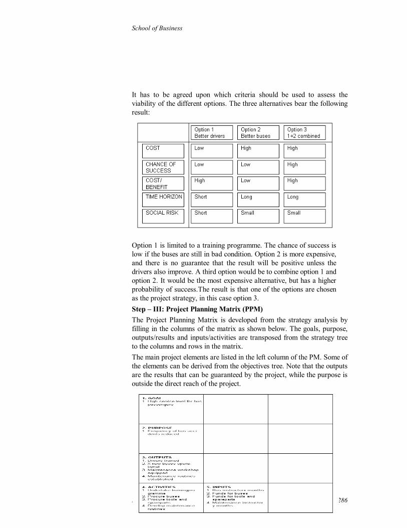
School of Business
Economic Development and Planning Page-286
It has to be agreed upon which criteria should be used to assess the viability of the different options. The three alternatives bear the following result: Option 1 is limited to a training programme. The chance of success is low if the buses are still in bad condition. Option 2 is more expensive, and there is no guarantee that the result will be positive unless the drivers also improve. A third option would be to combine option 1 and option 2. It would be the most expensive alternative, but has a higher probability of success.The result is that one of the options are chosen as the project strategy, in this case option 3. Step – III: Project Planning Matrix (PPM) The Project Planning Matrix is developed from the strategy analysis by filling in the columns of the matrix as shown below. The goals, purpose, outputs/results and inputs/activities are transposed from the strategy tree to the columns and rows in the matrix. The main project elements are listed in the left column of the PM. Some of the elements can be derived from the objectives tree. Note that the outputs are the results that can be guaranteed by the project, while the purpose is outside the direct reach of the project.
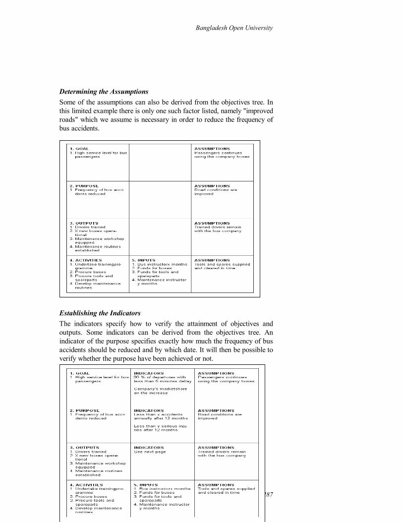
Bangladesh Open University
Unit-5 Page-287
Determining the Assumptions Some of the assumptions can also be derived from the objectives tree. In this limited example there is only one such factor listed, namely "improved roads" which we assume is necessary in order to reduce the frequency of bus accidents. Establishing the Indicators The indicators specify how to verify the attainment of objectives and outputs. Some indicators can be derived from the objectives tree. An indicator of the purpose specifies exactly how much the frequency of bus accidents should be reduced and by which date. It will then be possible to verify whether the purpose have been achieved or not.
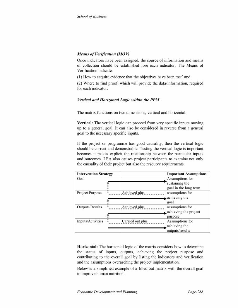
School of Business
Economic Development and Planning Page-288
Means of Verification (MOV) Once indicators have been assigned, the source of information and means of collection should be established fore each indicator. The Means of Verification indicate: (1) How to acquire evidence that the objectives have been met’ and (2) Where to find proof, which will provide the data/information, required for each indicator. Vertical and Horizontal Logic within the PPM
The matrix functions on two dimensions, vertical and horizontal. Vertical: The vertical logic can proceed from very specific inputs moving up to a general goal. It can also be considered in reverse from a general goal to the necessary specific inputs. If the project or programme has good causality, then the vertical logic should be correct and demonstrable. Testing the vertical logic is important becomes it makes explicit the relationship between the particular inputs and outcomes. LFA also causes project participants to examine not only the causality of their project but also the resource requirements. Intervention Strategy Important Assumptions Goal
Assumptions for sustaining the goal in the long term
Project Purpose Achieved plus assumptions for achieving the goal
Outputs/Results Achieved plus assumptions for achieving the project purpose
Inputs/Activities Carried out plus Assumptions for achieving the outputs/results
Horizontal: The horizontal logic of the matrix considers how to determine the status of inputs, outputs, achieving the project purpose and contributing to the overall goal by listing the indicators and verification and the assumptions overarching the project implementation. Below is a simplified example of a filled out matrix with the overall goal to improve human nutrition.

Bangladesh Open University
Unit-5 Page-289
Narrative Summary
Objectively Verifiable Indicators
Means of Verification
Important Assumptions
GOAL/ OBJECTIVE Improving human nutrition in X
Improved human nutrition
Quantitative measures available from public sources or records of the project
Having more food produced will increase availability and improve nutrition
PROJECT PURPOSE increase food production
Increased food production
Quantitative measures available from public sources or records of the project
Better yields will lead to increased production
OUTPUTS/ RESULTS increased yields of vegetables
Increased quantities of vegetables
Quantitative measures available from public sources or records of the project
Using irrigation water will increase yields
INPUTS/ ACTIVITIES Irrigation water
Irrigation water Quantitative measures available from public sources or records of the project
Irrigation water is available and can be distributed The increased yields will be available to the people
Step – IV: Implementation
The operational phase of a project commences when implementing activities begin in order to achieve the expected outputs/results. In many cases this may be one or two years after the project concept had been established at the end of the design phase (as laid down in the PPM of the project appraisal). In the meantime framework conditions may have changed, so that a verification of the PPM must take place during the operational planning. The project purpose and development goal, however, should be altered only in exceptional cases when major changes have occurred.
Implementation should have a plan of operations i.e. the detailed plan for the implementation of project. It is established by the project team and will be documented as:
workplans / work schedules

School of Business
Economic Development and Planning Page-290
project budget / resources plans
personnel plans
material and equipment plan / procurement plan / staff training plans.
The work plan and the project budget constitute the core of the Plan of Operations.
Weaknesses with Logical Frameworks
LFA provide a valuable set of tools for project designing, but they also have a number of weaknesses. Such weaknesses include, but are not limited to the following:
1. One of the main criticisms that project designers have of the LFA approach is that it begins by identifying problems. There are three problems that emerge from beginning with problems:
Beginning with the problem analysis often produces poor results because the initial negative focus pervades the rest of the LFA process. This often results in limited vision of potential solutions.
Beginning with the problem analysis can be particularly serious problem in cultures that consider it inappropriate to openly discuss problems or criticise.
Beginning with the problem analysis is not suited to situations where there is a great deal of uncertainty or where agreement cannot be reached on the main problem. The LFA approach assumes the nature of the problems can be readily determined at the beginning of the planning process. This does not allow for an exploratory style project that seeks to learn from experience.
2. The LFA is often developed and used rigidly. This can stifle innovative thinking and adaptive management.
3. LFAs are often developed after the project has been designed rather than used as the basis for design. The use of the LFA late in the design process can often be attributed to:
a lack of understanding of the LFA approach
the LFA is seen as a requirement of funding
agencies and not as a design or management tool.
4. LFAs do not readily enable monitoring unintended consequences.

Bangladesh Open University
Unit-5 Page-291
5. LFAs are rarely considered by project managers to be a key planning tool.

School of Business
Economic Development and Planning Page-292
Conclusions
The logical framework approach provides a powerful set of tools for designing projects and project evaluations. However, like all tools, LFAs are not the complete answer to effective project designing. LFAs are best used towards the end of the project design cycle after information has been collected and analysed, needs assessed, views of stakeholders sought and the external environment of the project understood.

Bangladesh Open University
Unit-5 Page-293
Questions for Review Multiple Choice Questions 1. The top of the problem tree is
a. the main problem or the effect b. causes c. root causes d. objective
2. The lower levels of the problem tree are : a. the main problem or the effect b. causes c. Means of verification d. indicators
3. The top of the objective tree is a. root causes b. main problem or the effect c. the end desired d. means to achieve the end
4. A matrix in LFA functions on a. four dimensions b. three dimensions b. multi-dimensions d. two dimensions
Answers: 1. a, 2. b, 3. c and 4. d
Short Questions
1. What are the advantages of using LFA? 2. What is stakeholder analysis? 3. What are the vertical and horizontal logics within project planning
matrix? 4. What do the means of verification indicate?
Essay-type Questions 1. The logical framework approach provides a powerful set of tools
for designing projects and project evaluations – explain.
2. Do you agree with the view that LFAs are not the complete answer to effective project designing?
Further Reading 1. Gesellschaft für Technische Zusammenarbeit (GTZ). 1991.
Methods and Instruments for Project Planning and Implementation. Eschborn: Germany.
2. GTZ. 1988. ZOPP (An Introduction to the Method). Eschborn, Germany.
3. GTZ. 1988. ZOPP in Brief. Eschborn, Germany. 4. ITAD Ltd (1996) "The logical framework approach - a project
management tool". 5. IUCN (1997) Draft PDG Guidelines: A guide to the development,
review and further processing of projects in IUCN. 6. Prescott-Allen R. (1997) The Barometer of Sustainability. IUCN
Switzerland.