University of Massachusetts AmherstScholarWorks@UMass AmherstComputer Science Department Faculty PublicationSeries Computer Science

2006

STATISTICAL MODELS AND ANALYSISTECHNIQUES FOR LEARNING INRELATIONAL DATAJennifer NevilleUniversity of Massachusetts Amherst

Follow this and additional works at: https://scholarworks.umass.edu/cs_faculty_pubs

Part of the Computer Sciences Commons

This Article is brought to you for free and open access by the Computer Science at ScholarWorks@UMass Amherst. It has been accepted for inclusionin Computer Science Department Faculty Publication Series by an authorized administrator of ScholarWorks@UMass Amherst. For more information,please contact scholarworks@library.umass.edu.

Recommended CitationNeville, Jennifer, "STATISTICAL MODELS AND ANALYSIS TECHNIQUES FOR LEARNING IN RELATIONAL DATA"(2006). Computer Science Department Faculty Publication Series. 127.Retrieved from https://scholarworks.umass.edu/cs_faculty_pubs/127

STATISTICAL MODELS AND ANALYSIS TECHNIQUESFOR LEARNING IN RELATIONAL DATA

A Dissertation Presented

by

JENNIFER NEVILLE

Submitted to the Graduate School of theUniversity of Massachusetts Amherst in partial fulfillment

of the requirements for the degree of

DOCTOR OF PHILOSOPHY

September 2006

Computer Science

c© Copyright by Jennifer Neville 2006

All Rights Reserved

STATISTICAL MODELS AND ANALYSIS TECHNIQUESFOR LEARNING IN RELATIONAL DATA

A Dissertation Presented

by

JENNIFER NEVILLE

Approved as to style and content by:

David Jensen, Chair

Andrew Barto, Member

Andrew McCallum, Member

Foster Provost, Member

John Staudenmayer, Member

W. Bruce Croft, Department ChairComputer Science

To the one who didn’t see the beginning, the one who didn’t see theend, and the one who was there for me throughout.

ACKNOWLEDGMENTS

First, I would like to express my deepest gratitude to my advisor, David Jensen.

I cannot thank him enough for introducing me to the exciting world of research—it

certainly has changed my life. Working with David has always been a delightful,

rewarding experience. He provided a research environment in which I could thrive—

where the pursuit of discovery was fostered through collaborative exploration rather

than competitive isolation. During my tenure at UMass, David has imparted innu-

merable lessons, ranging from invaluable advice on the intangible art of science, to

practical instruction on research, writing, and presentation, to insightful guidance on

academia and politics. Without his support, encouragement, and tutelage, I would

certainly not be where I am today. He is more than just a great advisor, he is a

friend, and that combination has made the past six years seem more like six months.

It’s hard to believe it’s coming to an end.

I would also like to thank the other members of my committee: Andy Barto, An-

drew McCallum, Foster Provost, and John Staudenmayer. Their helpful comments

and technical guidance facilitated the process, especially in light of my simultaneous

two-body search. Moreover, I greatly appreciate the assistance that Foster and An-

drew have offered throughout the years, even before I started my thesis. Exposure to

their supplementary views helped to broaden and deepen my sense of research and

academia in general and statistical relational learning in particular.

During my internship at AT&T Labs, working with Daryl Pregibon and Chris

Volinsky, I developed an appreciation for real-world applications and massive datasets.

This interest underlies much of the work in this thesis, in that efficient algorithms

and understandable models are two key components of applied data mining research.

v

In addition, Daryl and Chris have been wonderful mentors, both officially and unoffi-

cially. Daryl cultivated my interdisciplinary nature—as he continually questioned the

modeling choices of computer scientists and the computation choices of statisticians.

I hope to live up to his example as I start my joint appointment in CS and Statistics

and I will always think of him when I can’t remember what temporary data is stored

in my files named t, tt, and ttt.

I would like to express my appreciation to my collaborators at NASD: John Ko-

moroske, Henry Goldberg, and Kelly Palmer. The NASD fraud detection task is a

fascinating real-world problem, which has been a continual source of motivation and

often a harsh reality check. My work on the NASD project reminded me how inspir-

ing real-world applications can be. In addition, I am indebted to them for providing

such a compelling example for use throughout this thesis.

The work in this thesis has been directly impacted by my many collaborations in

the Knowledge Discovery Laboratory. I would like to thank Hannah Blau, Andy Fast,

Ross Fairgrieve, Lisa Friedland, Brian Gallagher, Amy McGovern, Michael Hay, Matt

Rattigan, and Ozgur Simsek for their excellent input and feedback. I am also indebted

to the invaluable assistance of the KDL technical staff: Matt Cornell, Cindy Loiselle,

and Agustin Schapira. All the members of KDL have been both friends and colleagues.

They made my graduate life not only bearable, but also rewarding and fun—as we saw

each other through arduous paper deadlines, frustrating database problems, puzzling

research findings, marathon pair-programming sessions, and countless practice talks.

Next, there are the friends who helped me maintain my sanity through the dif-

ficult coursework, research plateaus, and emotional challenges that inevitably occur

during graduate school. I couldn’t have done it without Ozgur Simsek and Pippin

Wolfe—they were always willing to offer insightful research advice and unquestioning

moral support. And what can I say to the other good friends I made at UMass?

Brian Gallagher, Kat Hanna, Michael Hay, Brent Heeringa, Amy McGovern, Nandini

vi

Natarajan, Matt Rattigan, Agustin Schapira and David Stracuzzi—thanks for all the

cube-side discussions, Rao’s coffee breaks, campus walks, and conference beers.

I owe an enormous amount to my family who set the foundation for this work. To

my father, who taught me how to ask why and to my mother, who listened patiently to

all my wonderings thereafter. To my stepdaughters Naomi and Kristin, who willingly

endured all my hours in front of the computer and never-ending bowls of noodles

when we were too busy to cook. To my son Jackson, who slept enough over the past

two months to give me time to finish writing. And to my husband Jim, for being my

joy, my strength, and my continuity.

Lastly, this work was supported by a National Science Foundation Graduate Re-

search Fellowship, an AT&T Labs Graduate Research Fellowship, and by DARPA

and AFRL under contract numbers HR0011-04-1-0013 and F30602-01-2-0566.

vii

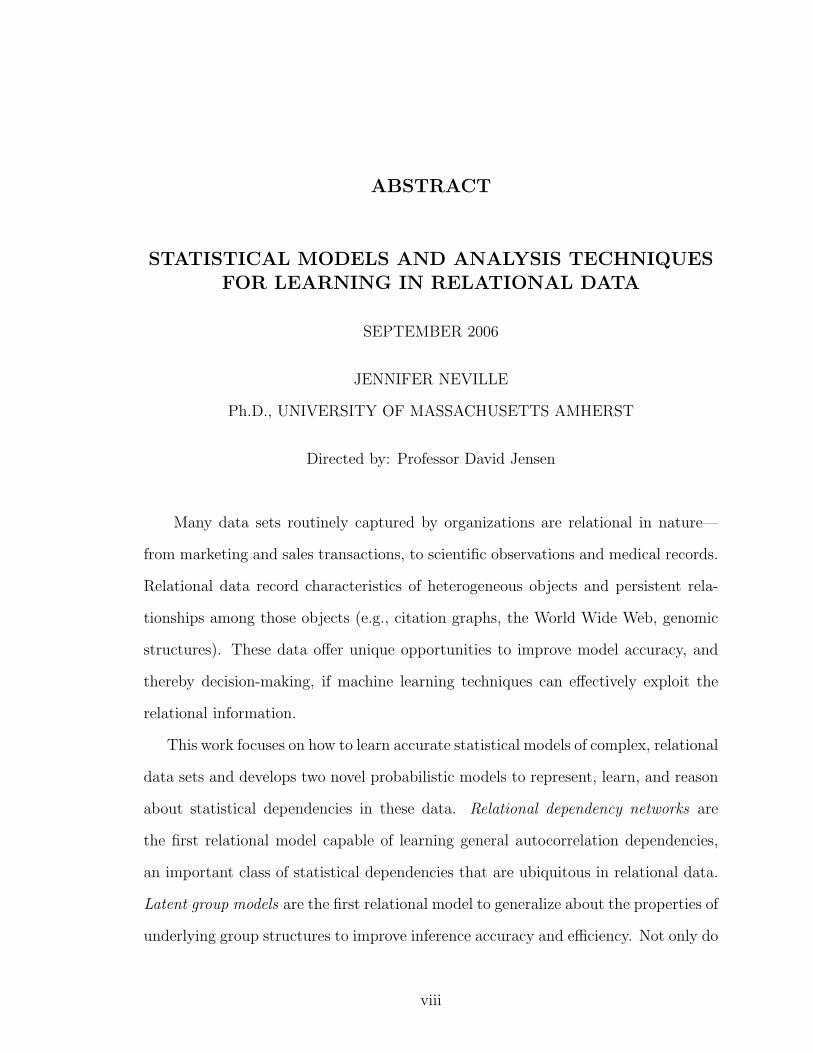
ABSTRACT

STATISTICAL MODELS AND ANALYSIS TECHNIQUESFOR LEARNING IN RELATIONAL DATA

SEPTEMBER 2006

JENNIFER NEVILLE

Ph.D., UNIVERSITY OF MASSACHUSETTS AMHERST

Directed by: Professor David Jensen

Many data sets routinely captured by organizations are relational in nature—

from marketing and sales transactions, to scientific observations and medical records.

Relational data record characteristics of heterogeneous objects and persistent rela-

tionships among those objects (e.g., citation graphs, the World Wide Web, genomic

structures). These data offer unique opportunities to improve model accuracy, and

thereby decision-making, if machine learning techniques can effectively exploit the

relational information.

This work focuses on how to learn accurate statistical models of complex, relational

data sets and develops two novel probabilistic models to represent, learn, and reason

about statistical dependencies in these data. Relational dependency networks are

the first relational model capable of learning general autocorrelation dependencies,

an important class of statistical dependencies that are ubiquitous in relational data.

Latent group models are the first relational model to generalize about the properties of

underlying group structures to improve inference accuracy and efficiency. Not only do

viii

these two models offer performance gains over current relational models, but they also

offer efficiency gains which will make relational modeling feasible for large, relational

datasets where current methods are computationally intensive, if not intractable.

We also formulate of a novel analysis framework to analyze relational model per-

formance and ascribe errors to model learning and inference procedures. Within this

framework, we explore the effects of data characteristics and representation choices

on inference accuracy and investigate the mechanisms behind model performance. In

particular, we show that the inference process in relational models can be a signif-

icant source of error and that relative model performance varies significantly across

different types of relational data.

ix

TABLE OF CONTENTS

Page

ACKNOWLEDGMENTS . . . . . . . . . . . . . . . . . . . . . . . . . . . . . . . . . . . . . . . . . . . . . v

ABSTRACT . . . . . . . . . . . . . . . . . . . . . . . . . . . . . . . . . . . . . . . . . . . . . . . . . . . . . . . . .viii

LIST OF TABLES . . . . . . . . . . . . . . . . . . . . . . . . . . . . . . . . . . . . . . . . . . . . . . . . . . .xiii

LIST OF FIGURES . . . . . . . . . . . . . . . . . . . . . . . . . . . . . . . . . . . . . . . . . . . . . . . . . .xiv

CHAPTER

1. INTRODUCTION . . . . . . . . . . . . . . . . . . . . . . . . . . . . . . . . . . . . . . . . . . . . . . . . . 1

1.1 Contributions . . . . . . . . . . . . . . . . . . . . . . . . . . . . . . . . . . . . . . . . . . . . . . . . . . . . 71.2 Thesis Outline . . . . . . . . . . . . . . . . . . . . . . . . . . . . . . . . . . . . . . . . . . . . . . . . . . . 9

2. MODELING RELATIONAL DATA . . . . . . . . . . . . . . . . . . . . . . . . . . . . . . . 11

2.1 Relational Data . . . . . . . . . . . . . . . . . . . . . . . . . . . . . . . . . . . . . . . . . . . . . . . . . 112.2 Relational Autocorrelation . . . . . . . . . . . . . . . . . . . . . . . . . . . . . . . . . . . . . . . . 122.3 Tasks . . . . . . . . . . . . . . . . . . . . . . . . . . . . . . . . . . . . . . . . . . . . . . . . . . . . . . . . . . 162.4 Sampling . . . . . . . . . . . . . . . . . . . . . . . . . . . . . . . . . . . . . . . . . . . . . . . . . . . . . . . 182.5 Models . . . . . . . . . . . . . . . . . . . . . . . . . . . . . . . . . . . . . . . . . . . . . . . . . . . . . . . . . 20

2.5.1 Individual Inference Models . . . . . . . . . . . . . . . . . . . . . . . . . . . . . . . . . 202.5.2 Collective Inference Models . . . . . . . . . . . . . . . . . . . . . . . . . . . . . . . . . 212.5.3 Probabilistic Relational Models . . . . . . . . . . . . . . . . . . . . . . . . . . . . . 22

3. RELATIONAL DEPENDENCY NETWORKS . . . . . . . . . . . . . . . . . . . . 27

3.1 Dependency Networks . . . . . . . . . . . . . . . . . . . . . . . . . . . . . . . . . . . . . . . . . . . . 29

3.1.1 DN Representation . . . . . . . . . . . . . . . . . . . . . . . . . . . . . . . . . . . . . . . . 313.1.2 DN Learning . . . . . . . . . . . . . . . . . . . . . . . . . . . . . . . . . . . . . . . . . . . . . 323.1.3 DN Inference . . . . . . . . . . . . . . . . . . . . . . . . . . . . . . . . . . . . . . . . . . . . . 33

x

3.2 Relational Dependency Networks . . . . . . . . . . . . . . . . . . . . . . . . . . . . . . . . . . 33

3.2.1 RDN Representation . . . . . . . . . . . . . . . . . . . . . . . . . . . . . . . . . . . . . . . 343.2.2 RDN Learning . . . . . . . . . . . . . . . . . . . . . . . . . . . . . . . . . . . . . . . . . . . . 36

3.2.2.1 Conditional Relational Learners . . . . . . . . . . . . . . . . . . . . . 403.2.2.2 Queries . . . . . . . . . . . . . . . . . . . . . . . . . . . . . . . . . . . . . . . . . . 44

3.2.3 RDN Inference . . . . . . . . . . . . . . . . . . . . . . . . . . . . . . . . . . . . . . . . . . . . 45

3.3 Experimental Evaluation . . . . . . . . . . . . . . . . . . . . . . . . . . . . . . . . . . . . . . . . . 49

3.3.1 Synthetic Data Experiments . . . . . . . . . . . . . . . . . . . . . . . . . . . . . . . . 49

3.3.1.1 RDN Learning . . . . . . . . . . . . . . . . . . . . . . . . . . . . . . . . . . . . 503.3.1.2 RDN Inference . . . . . . . . . . . . . . . . . . . . . . . . . . . . . . . . . . . . 52

3.3.2 Empirical Data Experiments . . . . . . . . . . . . . . . . . . . . . . . . . . . . . . . . 57

3.3.2.1 RDN Models . . . . . . . . . . . . . . . . . . . . . . . . . . . . . . . . . . . . . 593.3.2.2 Prediction . . . . . . . . . . . . . . . . . . . . . . . . . . . . . . . . . . . . . . . . 63

3.4 Related Work . . . . . . . . . . . . . . . . . . . . . . . . . . . . . . . . . . . . . . . . . . . . . . . . . . . 67

3.4.1 Probabilistic Relational Models . . . . . . . . . . . . . . . . . . . . . . . . . . . . . 673.4.2 Probabilistic Logic Models . . . . . . . . . . . . . . . . . . . . . . . . . . . . . . . . . . 703.4.3 Ad hoc Collective Models . . . . . . . . . . . . . . . . . . . . . . . . . . . . . . . . . . 71

3.5 Conclusion . . . . . . . . . . . . . . . . . . . . . . . . . . . . . . . . . . . . . . . . . . . . . . . . . . . . . 72

4. LATENT GROUP MODELS . . . . . . . . . . . . . . . . . . . . . . . . . . . . . . . . . . . . . 74

4.1 Latent Group Models . . . . . . . . . . . . . . . . . . . . . . . . . . . . . . . . . . . . . . . . . . . . 78

4.1.1 LGM Representation . . . . . . . . . . . . . . . . . . . . . . . . . . . . . . . . . . . . . . 784.1.2 LGM Learning . . . . . . . . . . . . . . . . . . . . . . . . . . . . . . . . . . . . . . . . . . . . 814.1.3 LGM Inference . . . . . . . . . . . . . . . . . . . . . . . . . . . . . . . . . . . . . . . . . . . . 84

4.2 Experimental Evaluation . . . . . . . . . . . . . . . . . . . . . . . . . . . . . . . . . . . . . . . . . 84

4.2.1 Synthetic Data Experiments . . . . . . . . . . . . . . . . . . . . . . . . . . . . . . . . 854.2.2 Empirical Data Experiments . . . . . . . . . . . . . . . . . . . . . . . . . . . . . . . . 89

4.3 Related Work . . . . . . . . . . . . . . . . . . . . . . . . . . . . . . . . . . . . . . . . . . . . . . . . . . . 93

4.3.1 Modeling Coordinating Objects . . . . . . . . . . . . . . . . . . . . . . . . . . . . . 944.3.2 Modeling Communities . . . . . . . . . . . . . . . . . . . . . . . . . . . . . . . . . . . . . 95

xi

4.3.3 Discussion . . . . . . . . . . . . . . . . . . . . . . . . . . . . . . . . . . . . . . . . . . . . . . . . 96

4.4 Conclusion . . . . . . . . . . . . . . . . . . . . . . . . . . . . . . . . . . . . . . . . . . . . . . . . . . . . . 97

5. BIAS/VARIANCE ANALYSIS . . . . . . . . . . . . . . . . . . . . . . . . . . . . . . . . . . . 99

5.1 Conventional Approach . . . . . . . . . . . . . . . . . . . . . . . . . . . . . . . . . . . . . . . . . . 1005.2 Relational framework . . . . . . . . . . . . . . . . . . . . . . . . . . . . . . . . . . . . . . . . . . . 1015.3 Experimental Evaluation . . . . . . . . . . . . . . . . . . . . . . . . . . . . . . . . . . . . . . . . 105

5.3.1 RDN Analysis . . . . . . . . . . . . . . . . . . . . . . . . . . . . . . . . . . . . . . . . . . . 1065.3.2 LGM Analysis . . . . . . . . . . . . . . . . . . . . . . . . . . . . . . . . . . . . . . . . . . . 111

5.4 Conclusion . . . . . . . . . . . . . . . . . . . . . . . . . . . . . . . . . . . . . . . . . . . . . . . . . . . . 114

6. CONCLUSION . . . . . . . . . . . . . . . . . . . . . . . . . . . . . . . . . . . . . . . . . . . . . . . . . . 116

6.1 Contributions . . . . . . . . . . . . . . . . . . . . . . . . . . . . . . . . . . . . . . . . . . . . . . . . . . 1166.2 Future Work . . . . . . . . . . . . . . . . . . . . . . . . . . . . . . . . . . . . . . . . . . . . . . . . . . . 1196.3 Conclusion . . . . . . . . . . . . . . . . . . . . . . . . . . . . . . . . . . . . . . . . . . . . . . . . . . . . 121

APPENDIX: . . . . . . . . . . . . . . . . . . . . . . . . . . . . . . . . . . . . . . . . . . . . . . . . . . . . . . . 123

A.1 Datasets . . . . . . . . . . . . . . . . . . . . . . . . . . . . . . . . . . . . . . . . . . . . . . . . . . . . . . 123

A.1.1 RDN Synthetic Data . . . . . . . . . . . . . . . . . . . . . . . . . . . . . . . . . . . . . 123A.1.2 LGM Synthetic Data . . . . . . . . . . . . . . . . . . . . . . . . . . . . . . . . . . . . . 128A.1.3 Real World Datasets . . . . . . . . . . . . . . . . . . . . . . . . . . . . . . . . . . . . . . 129

BIBLIOGRAPHY . . . . . . . . . . . . . . . . . . . . . . . . . . . . . . . . . . . . . . . . . . . . . . . . . . 133

xii

LIST OF TABLES

Table Page

3.1 RDN learning algorithm. . . . . . . . . . . . . . . . . . . . . . . . . . . . . . . . . . . . . . . . . . 41

3.2 RDN inference algorithm. . . . . . . . . . . . . . . . . . . . . . . . . . . . . . . . . . . . . . . . . 48

3.3 Number of attributes/features used by RDNs and RMNs. . . . . . . . . . . . . 67

xiii

LIST OF FIGURES

Figure Page

1.1 NASD relational data schema. . . . . . . . . . . . . . . . . . . . . . . . . . . . . . . . . . . . . . . 2

1.2 Example NASD database table. . . . . . . . . . . . . . . . . . . . . . . . . . . . . . . . . . . . . 3

1.3 Example NASD database fragment. . . . . . . . . . . . . . . . . . . . . . . . . . . . . . . . . . 4

2.1 Time series autocorrelation example. . . . . . . . . . . . . . . . . . . . . . . . . . . . . . . . 13

2.2 Example NASD database fragment with broker fraud labels. . . . . . . . . . . . 16

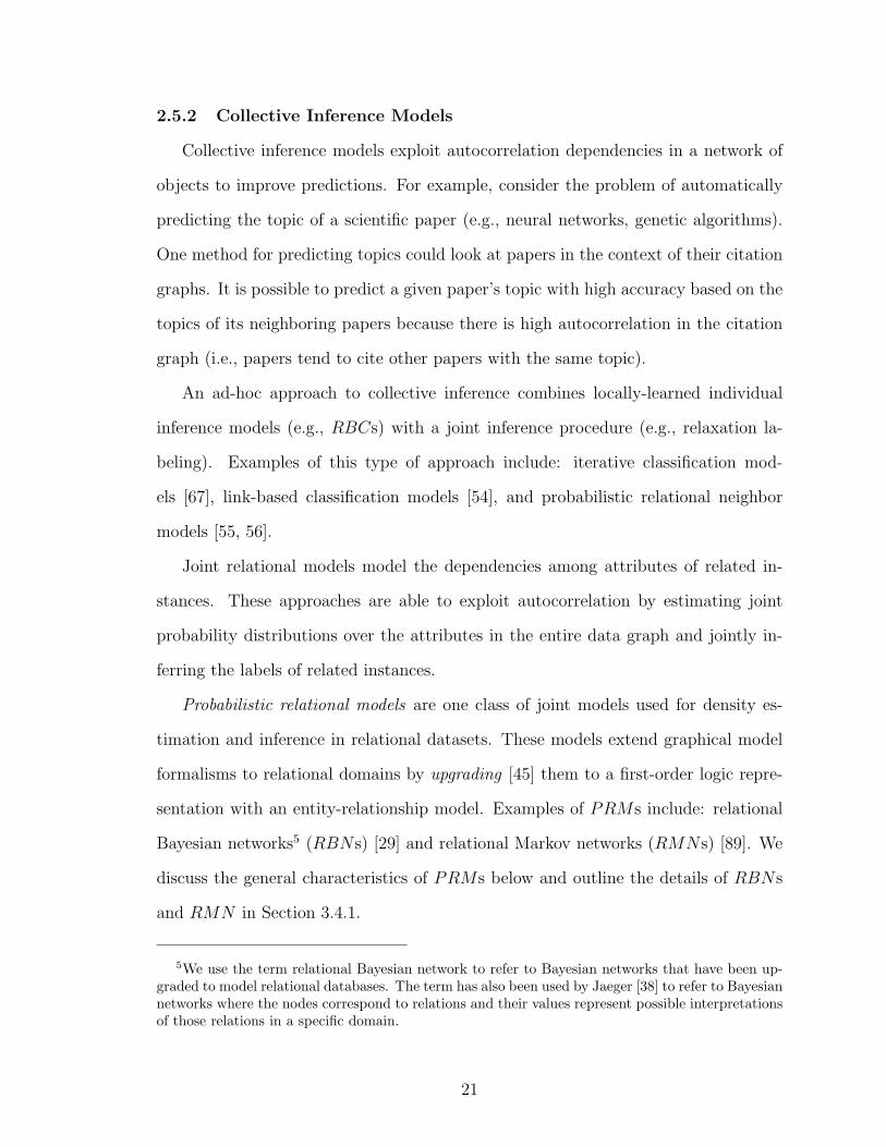
2.3 Example PRM (a) data graph and (b) model graph. . . . . . . . . . . . . . . . . . 23

2.4 Example PRM inference graph. . . . . . . . . . . . . . . . . . . . . . . . . . . . . . . . . . . . 26

3.1 Example DN . . . . . . . . . . . . . . . . . . . . . . . . . . . . . . . . . . . . . . . . . . . . . . . . . . . . 32

3.2 Example RPT to predict machine-learning paper topic. . . . . . . . . . . . . . . . 43

3.3 (a) Example QGraph query, and (b) matching subgraph. . . . . . . . . . . . . . . 45

3.4 Evaluation of RDNRPT (top row) and RDNRBC (bottom row)learning. . . . . . . . . . . . . . . . . . . . . . . . . . . . . . . . . . . . . . . . . . . . . . . . . . . . . 51

3.5 Evaluation of RDNRPT (top row) and RDNRBC (bottom row)inference. . . . . . . . . . . . . . . . . . . . . . . . . . . . . . . . . . . . . . . . . . . . . . . . . . . . . 55

3.6 Gibbs convergence rates for five different trials of RDNRPT (top row)and RDNRBC (bottom row). . . . . . . . . . . . . . . . . . . . . . . . . . . . . . . . . . . . 58

3.7 RDN for the Cora dataset. . . . . . . . . . . . . . . . . . . . . . . . . . . . . . . . . . . . . . . . 60

3.8 RDN for the Gene dataset. . . . . . . . . . . . . . . . . . . . . . . . . . . . . . . . . . . . . . . . 61

3.9 RDN for the IMDb dataset. . . . . . . . . . . . . . . . . . . . . . . . . . . . . . . . . . . . . . . 62

xiv

3.10 RDN for the NASD dataset. . . . . . . . . . . . . . . . . . . . . . . . . . . . . . . . . . . . . . . 63

3.11 RDN for the WebKB dataset. . . . . . . . . . . . . . . . . . . . . . . . . . . . . . . . . . . . . . 63

3.12 AUC results for (a) RDNRPT and RPT and (b) RDNRBC andRBC. . . . . . . . . . . . . . . . . . . . . . . . . . . . . . . . . . . . . . . . . . . . . . . . . . . . . . . . 65

4.1 Example NASD database fragment and group structure. . . . . . . . . . . . . . . 75

4.2 Example WebKB fragment and group structure. . . . . . . . . . . . . . . . . . . . . . 76

4.3 LGM graphical representation. . . . . . . . . . . . . . . . . . . . . . . . . . . . . . . . . . . . . 81

4.4 Sample synthetic dataset. . . . . . . . . . . . . . . . . . . . . . . . . . . . . . . . . . . . . . . . . . 87

4.5 Evaluation of LGM inference. . . . . . . . . . . . . . . . . . . . . . . . . . . . . . . . . . . . . . 88

4.6 LGM performance when the class label is the only availableattribute. . . . . . . . . . . . . . . . . . . . . . . . . . . . . . . . . . . . . . . . . . . . . . . . . . . . . 92

4.7 LGM performance when additional attributes are included. . . . . . . . . . . . 94

5.1 Distributions of model predictions. . . . . . . . . . . . . . . . . . . . . . . . . . . . . . . . . 104

5.2 Bias/variance analysis on RDNRPT synthetic data. . . . . . . . . . . . . . . . . . . 107

5.3 Bias/variance analysis on RDNRBC synthetic data. . . . . . . . . . . . . . . . . . 110

5.4 Bias/variance analysis on LGM synthetic data. . . . . . . . . . . . . . . . . . . . . . 112

A.1 RPT0.25 used for synthetic data generation with lowautocorrelation. . . . . . . . . . . . . . . . . . . . . . . . . . . . . . . . . . . . . . . . . . . . . . 125

A.2 RPT0.50 used for synthetic data generation with mediumautocorrelation. . . . . . . . . . . . . . . . . . . . . . . . . . . . . . . . . . . . . . . . . . . . . . 126

A.3 RPT0.75 used for synthetic data generation with high autocorrelationlevels. . . . . . . . . . . . . . . . . . . . . . . . . . . . . . . . . . . . . . . . . . . . . . . . . . . . . . . 127

A.4 Data schemas for (a) Cora, (b) Gene, (c) IMDb, (d) NASD, and (e)WebKB. . . . . . . . . . . . . . . . . . . . . . . . . . . . . . . . . . . . . . . . . . . . . . . . . . . . . 131

xv

CHAPTER 1

INTRODUCTION

Many data sets routinely captured by businesses and organizations are relational in

nature—from marketing and sales transactions, to scientific observations and medical

records. Relational data record characteristics of heterogeneous objects (e.g., people,

places, and things) and persistent relationships among those objects. Examples of

relational data include citation graphs, the World Wide Web, genomic structures,

epidemiology data, and data on interrelated people, places, and events extracted

from text documents.

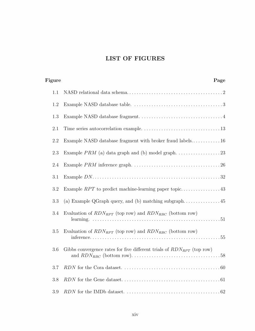
For example, consider the National Association of Securities Dealers’ (NASD)

Central Registration Depository system (CRD c©).1 The system contains data on ap-

proximately 3.4 million securities brokers, 360,000 branches, 25,000 firms, and 550,000

disclosure events, which record disciplinary information on brokers from customer

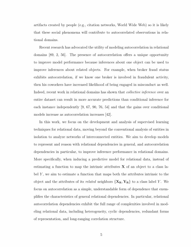
complaints to termination actions. Figure 1.1 shows the data schematically, includ-

ing frequency counts and example attributes for both entities and relations in a sample

of the CRD data. Relational data such as these are often stored in multiple tables,

with separate tables recording the attributes of different object types (e.g., brokers,

branches) and the relationships among objects (e.g., located-at).

In contrast, propositional data record characteristics of a single set of homogeneous

objects. Propositional data are often stored in a single database table, with each

row corresponding to a separate object (e.g. broker) and each column recording an

1See http://www.nasdbrokercheck.com.

1

Branch295,455

Disclosure384,944

Broker1,245,919

Firm16,047

Regulator61

BelongsTo295,455

LocatedAt1,945,942

WorkedFor2,820,426

FiledOn384,944

ReportedTo66,823

RegisteredWith248,757

Exchange

DateType

DBALocation

InstitutionLocation

BeginDateEndDate

Figure 1.1. NASD relational data schema.

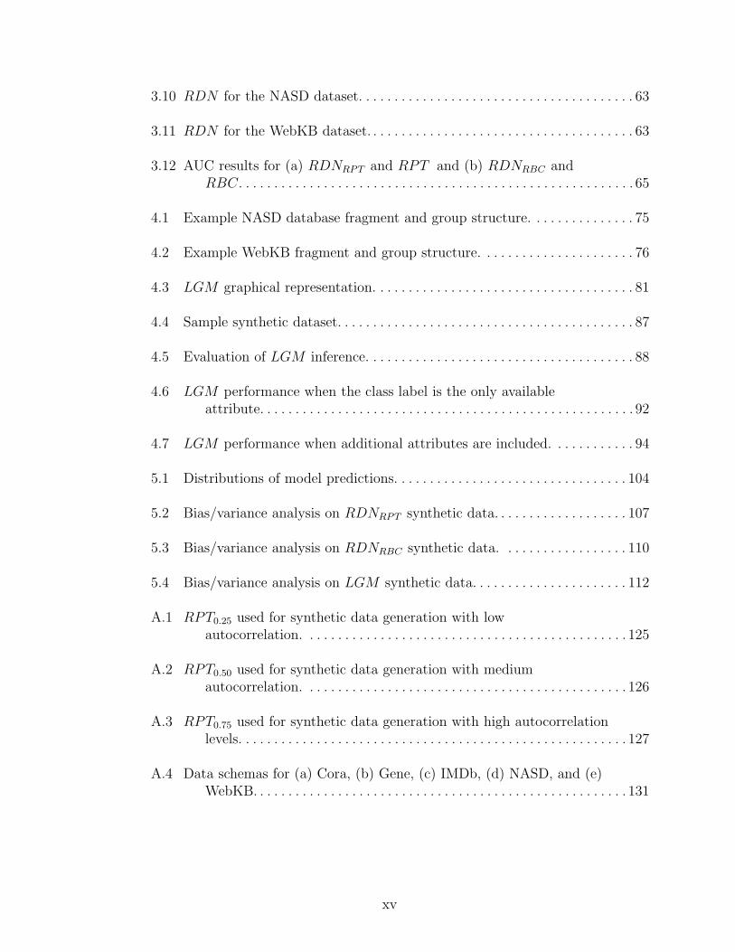
attribute of the objects (e.g. age). For example, Figure 1.2 depicts a propositional

table with hypothetical broker information.

Consider the task of identifying brokers involved in securities fraud faced by the

NASD [66]. NASD is the world’s largest private-sector securities regulator, with

responsibility for preventing and discovering misconduct among brokers such as fraud

and other violations of securities regulations. NASD currently identifies higher-risk

brokers using a set of handcrafted rules. However, we are interested in using supervised

learning techniques to automatically induce a predictive model of broker risk to use to

target NASD’s limited regulatory resources on brokers who are most likely to engage

in fraudulent behavior.

Supervised learning techniques are methods for automatically inducing a predic-

tive model from a set of training data. Over the past two decades, most machine

learning research focused on induction algorithms for propositional datasets. Propo-

sitional training data consist of pairs of class labels Y (e.g., is-higher-risk) and at-

tribute vectors X = X1, X2, ..., Xm (e.g., age, start-year). The task is to estimate

2

IsHigherRisk Series7Age StartYear CollegeDeg

+ Y25 1997 N

- N32 1982 N

- N24 2000 Y

- Y28 1995 Y

... ...... ... ...

...

...

...

...

...

...

Figure 1.2. Example NASD database table.

a function, given data from a number of training examples, that predicts a class label

value for any input attribute vector (i.e., f(x)→ y).

Algorithms for modeling propositional data assume that the training examples

are recorded in homogeneous structures (e.g., rows in a table, see Figure 1.2) but

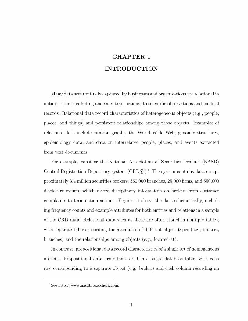
relational data are usually more varied and complex. For example, consider the rela-

tional data graph in Figure 1.3. Each broker has a different number of related objects,

resulting in diverse structures—some brokers have no disclosures while others have

many; some have few coworkers while others have many. Algorithms for propositional

data also assume the examples are independent and identically distributed (i.i.d.) but

relational data violate this assumption—the data have dependencies both as a result

of direct relations and through chaining multiple relations together. For example, in

Figure 1.3 brokers are not independent, they are related through the branches where

they work.

Relational data offer unique opportunities to boost model accuracy and to improve

decision-making quality if the algorithms can learn effectively from the additional

information the relationships provide. The power of relational data lies in combining

intrinsic information about objects in isolation with information about related objects

and the connections among those objects. For example, relational information is

often central to the task of fraud detection because fraud and malfeasance are social

3

BrokerBranch

Disclosure

Figure 1.3. Example NASD database fragment.

phenomena, communicated and encouraged by the presence of other individuals who

also wish to commit fraud (e.g., [11]).

In particular, the presence of autocorrelation provides a strong motivation for

using relational techniques for learning and inference. Autocorrelation is a statistical

dependency between the values of the same variable on related entities, which is a

nearly ubiquitous characteristic of relational datasets.2 For example, pairs of brokers

working at the same branch are more likely to share the same fraud status than

randomly selected pairs of brokers.

A number of widely occurring phenomena give rise to autocorrelation dependen-

cies. A hidden condition or event, whose influence is correlated among instances that

are closely located in time or space, can result in autocorrelated observations [63, 1].

Social phenomena, including social influence [57], diffusion [19], and homophily [61],

can also cause autocorrelated observations through their influence on social inter-

actions that govern the data generation process. Relational data often record in-

formation about people (e.g., organizational structure, email transactions) or about

2See Section 2.2 for a more formal definition of relational autocorrelation.

4

artifacts created by people (e.g., citation networks, World Wide Web) so it is likely

that these social phenomena will contribute to autocorrelated observations in rela-

tional domains.

Recent research has advocated the utility of modeling autocorrelation in relational

domains [89, 2, 56]. The presence of autocorrelation offers a unique opportunity

to improve model performance because inferences about one object can be used to

improve inferences about related objects. For example, when broker fraud status

exhibits autocorrelation, if we know one broker is involved in fraudulent activity,

then his coworkers have increased likelihood of being engaged in misconduct as well.

Indeed, recent work in relational domains has shown that collective inference over an

entire dataset can result in more accurate predictions than conditional inference for

each instance independently [9, 67, 90, 76, 54] and that the gains over conditional

models increase as autocorrelation increases [42].

In this work, we focus on the development and analysis of supervised learning

techniques for relational data, moving beyond the conventional analysis of entities in

isolation to analyze networks of interconnected entities. We aim to develop models

to represent and reason with relational dependencies in general, and autocorrelation

dependencies in particular, to improve inference performance in relational domains.

More specifically, when inducing a predictive model for relational data, instead of

estimating a function to map the intrinsic attributes X of an object to a class la-

bel Y , we aim to estimate a function that maps both the attributes intrinsic to the

object and the attributes of its related neighbors XR,YR to a class label Y . We

focus on autocorrelation as a simple, understandable form of dependence that exem-

plifies the characteristics of general relational dependencies. In particular, relational

autocorrelation dependencies exhibit the full range of complexities involved in mod-

eling relational data, including heterogeneity, cyclic dependencies, redundant forms

of representation, and long-ranging correlation structure.

5

In this thesis, we investigate the following hypothesis: Data characteristics

and representation choices interact to affect relational model performance

through their impact on learning and inference error. In particular, we eval-

uate different approaches to representing autocorrelation, explore the effects of at-

tribute and link structure on prediction accuracy, and investigate the mechanisms

behind model performance.

The contributions of this thesis include (1) the development of two novel proba-

bilistic relational models (PRMs)3 to represent arbitrary autocorrelation dependen-

cies and algorithms to learn these dependencies, and (2) the formulation of a novel

analysis framework to analyze model performance and ascribe errors to model learning

and inference procedures.

First, we present relational dependency networks (RDNs), an undirected graph-

ical model that can be used to represent and reason with cyclic dependencies in a

relational setting. RDNs use pseudolikelihood learning techniques to estimate an effi-

cient approximation of the full joint distribution of the attribute values in a relational

dataset.4 RDNs are the first PRM capable of learning autocorrelation dependen-

cies. RDNs also offer a relatively simple method for structure learning and parameter

estimation, which can result in models that are easier to understand and interpret.

Next, we present latent group models (LGMs), a directed graphical model that

models both the attribute and link structure in relational datasets. LGMs posit

groups of objects in the data—membership in these groups influences the observed

attributes of the objects, as well as the existence of relations among the objects.

LGMs are the first PRM to generalize about latent group properties and take ad-

vantage of those properties to improve inference accuracy.

3Several previous papers (e.g., [26, 29]) use the term probabilistic relational model to refer to aspecific model that is now often called a relational Bayesian network (Koller, personal communica-tion). In this thesis, we use PRM in its more recent and general sense.

4See Section 3.2.2 for a formal definition of pseudolikelihood estimation.

6

Finally, we develop a novel bias/variance analysis framework to explore the mecha-

nisms underlying model performance in relational domains. Conventional bias/variance

analysis associates model errors with aspects of the learning process. However, in

relational applications, the use of collective inference techniques introduces an ad-

ditional source of error—both through the use of approximate inference algorithms

and through variation in the availability of test set information. We account for this

source of error in a decomposition that associates error with aspects of both learning

and inference processes, showing that inference can be a significant source of error

and that models exhibit different types of errors as data characteristics are varied.

1.1 Contributions

This thesis investigates the connections between autocorrelation and improve-

ments in inference due to the use of probabilistic relational models and collective

inference procedures.

The primary contributions of this thesis are two-fold. First, a thorough inves-

tigation of autocorrelation and its impact on relational learning has improved our

understanding of the range and applicability of relational models. We compare

the performance of models that represent autocorrelation indirectly (i.e., LGMs) to

the performance of models that represent the observed autocorrelation directly (i.e.,

RDNs) and show that representation choices interact with dataset characteristics

and algorithm execution to affect performance. This indicates that properties other

than attribute correlation structure should be considered when choosing a model for

relational datasets.

Second, this work has improved the overall performance of relational models, in-

creasing both inference performance and model efficiency. In small datasets, where we

have the computational resources to apply current learning and inference techniques,

a better understanding of the effects of data characteristics on model performance can

7

increase the accuracy of the models. More specifically, we show that graph structure,

autocorrelation dependencies, and amount of test set labeling, affect relative model

performance. In larger datasets, where current learning and inference techniques are

computationally intensive, if not intractable, the efficiency gains offered by RDNs

and LGMs can make relational modeling both practical and feasible.

This thesis makes a number of theoretical and empirical contributions that we

outline below:

• Theoretical

– Development of relational dependency networks, a novel probabilistic rela-

tional model to efficiently learn arbitrary autocorrelation dependencies

∗ Proof of correspondence between consistent RDNs and relational Markov

networks5

∗ Proof of asymptotic properties of pseudolikelihood estimation in RDNs

– Development of latent group models, a novel probabilistic relational model

to generalize about latent group structures to improve inference accuracy

– Creation of novel bias/variance framework that decomposes relational model

errors into learning and inference components

• Empirical

– Validation of RDNs and LGMs on several real-world domains, including

a dataset of scientific papers, a collection of webpages, and data for a fraud

detection task

– Illustration of effects of representation choices on model performance using

synthetic datasets

5See Section 3.4.1 for a description of relational Markov networks (RMNs) [89].

8

– Illustration of effects of data characteristics on model performance using

synthetic datasets

– Investigation of errors introduced by collective inference processes using

synthetic datasets

1.2 Thesis Outline

There are three components to the thesis. In the first component, we develop

a probabilistic relation model capable of modeling arbitrary autocorrelation depen-

dencies. In the second component, we develop a probabilistic relational model that

incorporates group structure in a tractable manner to model observed autocorrelation.

In the third component, we propose a bias/variance analysis framework to evaluate

the effects of model representation and data characteristics on performance.

The remainder of this thesis is organized as follows. Chapter 2 reviews relevant

background material on relational data, tasks, and models. Chapter 3 describes re-

lational dependency networks (RDNs), outlines the RDN learning and inference

procedures, and presents empirical results on both real-world and synthetic datasets.

Chapter 4 describes latent group models (LGMs), outlines a learning and inference

procedure for a specific form of LGMs, and presents empirical results on both real-

world and synthetic datasets. Chapter 5 outlines a bias/variance framework for re-

lational models and presents empirical experiments on synthetic data, which explore

the mechanisms underlying model performance. Finally, we conclude in Chapter 6

with a review of the main contributions of the thesis and a discussion of extensions

and future work.

Some of this material has appeared previously in workshop and conference pa-

pers. The work on RDNs in Chapter 3 first appeared in Neville and Jensen [69]. It

later appeared in Neville and Jensen [70] and Neville and Jensen [74]. The work on

LGMs in Chapter 4 first appeared in Neville and Jensen [71], and later in Neville

9

and Jensen [72]. The bias/variance framework in Chapter 5 first appeared in Neville

and Jensen [73].

10

CHAPTER 2

MODELING RELATIONAL DATA

2.1 Relational Data

There are three nearly equivalent representations for relational datasets:

• Graphs—A directed, attributed hypergraph with V nodes representing objects

and E hyperedges representing relations, with one or more connected compo-

nents.

• Relational databases—A set of database tables with entities E and relations R.

Items of a common type are stored in a separate database table with one field

for each attribute.

• First-order logic knowledge bases—A set of first-order logic statements.

This work considers relational data represented as a typed, attributed data graph

GD = (VD, ED). To simplify discussion we will restrict our attention to binary links,

however the models and algorithms are applicable to more general hypergraphs.1 For

example, consider the data graph in Figure 1.3. The nodes VD represent objects in the

data (e.g., people, organizations, events) and the edges ED represent relations among

the objects (e.g., works-for, located-at). We use rectangles to represent objects and

dashed lines to represent relations.2

1The limitations imposed by binary links can usually by avoided by creating objects to representmore complex relations such as events [14].

2Later, we will use circles to represent random variables and solid lines to represent probabilisticdependencies in graphical representations of PRMs.

11

Each node vi ∈ VD and edge ej ∈ ED are associated with a type T (vi) =

tvi, T (ej) = tej

. This is depicted by node color in Figure 1.3. For example, blue

nodes represent people and green nodes represent organizations. Each item type

t ∈ T has a number of associated attributes Xt = (X t1, ..., X

tm) (e.g., age, gender).3

Consequently, each object v and link e are associated with a set of attribute values

determined by their type Xtvv = (X tv

v1, ..., Xtvvm), Xte

e = (X tee1, ..., X

teem′).

Relational data often have irregular structures and complex dependencies that

contradict the assumptions of conventional machine learning techniques. Algorithms

for propositional data assume that the data instances are recorded in homogeneous

structures (i.e., a fixed set of fields for each object), but relational data instances are

usually more varied and complex. For example, organizations each employ a different

number of people and customers each purchase a different number of products. The

ability to generalize across heterogeneous data instances is a defining characteristic

of relational learning algorithms. Algorithms designed for propositional data also as-

sume data instances are i.i.d.. Relational data, on the other hand, have dependencies

both as a result of direct relations (e.g., company subsidiaries) and through chaining

of multiple relations (e.g., employees at the same firm).

2.2 Relational Autocorrelation

Relational autocorrelation refers to a statistical dependency between values of the

same variable on related objects.4 More formally, we define relational autocorrelation

with respect to a set of related instance pairs PR related through paths of length l in

a set of edges ER: PR = (vi, vj) : eik1 , ek1k2 , ..., eklj ∈ ER, where ER = eij ⊆ E.

3We use the generic term “item” to refer to objects or links.

4We use the term autocorrelation in a more general sense than past work in econometrics(e.g., [63]) and spatial statistics (e.g., [13]). In this work, we use autocorrelation to refer to au-todependence among the values of a variable on related instances, including non-linear correlationamong continuous variables and dependence among discrete variables.

12

V5V4V3V2V1

X1 X2 X3 X4 X5

Y1 Y2 Y3 Y4 Y5

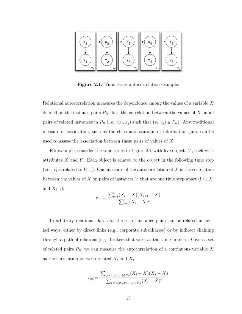
Figure 2.1. Time series autocorrelation example.

Relational autocorrelation measures the dependence among the values of a variable X

defined on the instance pairs PR. It is the correlation between the values of X on all

pairs of related instances in PR (i.e., (xi, xj) such that (vi, vj) ∈ PR). Any traditional

measure of association, such as the chi-square statistic or information gain, can be

used to assess the association between these pairs of values of X.

For example, consider the time series in Figure 2.1 with five objects V , each with

attributes X and Y . Each object is related to the object in the following time step

(i.e., Vi is related to Vi+1). One measure of the autocorrelation of X is the correlation

between the values of X on pairs of instances V that are one time step apart (i.e., Xi

and Xi+1):

rac =

∑4i=1(Xi − X)(Xi+1 − X)∑5

i=1(Xi − X)2

In arbitrary relational datasets, the set of instance pairs can be related in myr-

iad ways, either by direct links (e.g., corporate subsidiaries) or by indirect chaining

through a path of relations (e.g., brokers that work at the same branch). Given a set

of related pairs PR, we can measure the autocorrelation of a continuous variable X

as the correlation between related Xi and Xj:

rac =

∑ij s.t.(vi,vj)∈PR

(Xi − X)(Xj − X)∑i s.t.(vi,.)∨(.,vi)∈PR

(Xi − X)2

13

Alternatively for a binary variable X, we can measure the autocorrelation between

related Xi and Xj using Pearson’s contingency coefficient [84]:

rac =

√χ2

(N + χ2)=

√√√√ (n00n11−n01n10)2·N(n00+n01)(n10+n11)(n01+n11)(n00+n10)

(N + (n00n11−n01n10)2·N(n00+n01)(n10+n11)(n01+n11)(n00+n10)

)

where nab = |(xi, xj) : xi = a, xj = b, (vi, vj) ∈ PR| and N is the total number of

instances in PR.

A number of widely occurring phenomena give rise to autocorrelation dependen-

cies. Temporal and spatial locality often result in autocorrelated observations, due to

temporal or spatial dependence of measurement errors, or to the existence of a vari-

able whose influence is correlated among instances that are closely located in time or

space [63, 1]. Social phenomena such as social influence [57], diffusion processes [19],

and the principle of homophily [61] give rise to autocorrelated observations as well,

through their influence on social interactions that govern the data generation process.

Autocorrelation is a nearly ubiquitous characteristic of relational datasets. For

example, recent analysis of relational datasets has reported autocorrelation in the

following variables:

• Topics of hyperlinked web pages [9, 89]

• Industry categorization of corporations that share board members [67]

• Fraud status of cellular customers who call common numbers [22, 11]

• Topics of coreferent scientific papers [90, 69]

• Functions of colocated proteins in a cell [68]

• Box-office receipts of movies made by the same studio [40]

• Industry categorization of corporations that co-occur in news stories [2]

14

• Tuberculosis infection among people in close contact [29]

• Product/service adoption among customers in close communication [18, 35]

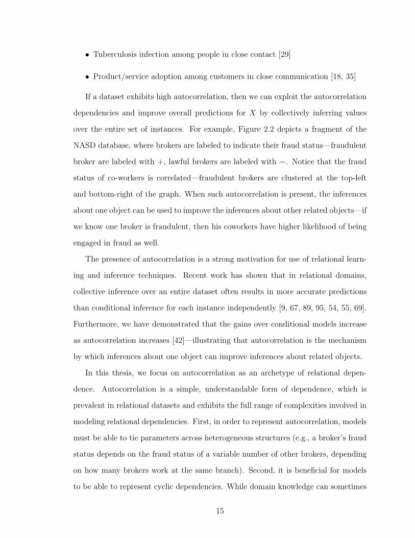
If a dataset exhibits high autocorrelation, then we can exploit the autocorrelation

dependencies and improve overall predictions for X by collectively inferring values

over the entire set of instances. For example, Figure 2.2 depicts a fragment of the

NASD database, where brokers are labeled to indicate their fraud status—fraudulent

broker are labeled with +, lawful brokers are labeled with −. Notice that the fraud

status of co-workers is correlated—fraudulent brokers are clustered at the top-left

and bottom-right of the graph. When such autocorrelation is present, the inferences

about one object can be used to improve the inferences about other related objects—if

we know one broker is fraudulent, then his coworkers have higher likelihood of being

engaged in fraud as well.

The presence of autocorrelation is a strong motivation for use of relational learn-

ing and inference techniques. Recent work has shown that in relational domains,

collective inference over an entire dataset often results in more accurate predictions

than conditional inference for each instance independently [9, 67, 89, 95, 54, 55, 69].

Furthermore, we have demonstrated that the gains over conditional models increase

as autocorrelation increases [42]—illustrating that autocorrelation is the mechanism

by which inferences about one object can improve inferences about related objects.

In this thesis, we focus on autocorrelation as an archetype of relational depen-

dence. Autocorrelation is a simple, understandable form of dependence, which is

prevalent in relational datasets and exhibits the full range of complexities involved in

modeling relational dependencies. First, in order to represent autocorrelation, models

must be able to tie parameters across heterogeneous structures (e.g., a broker’s fraud

status depends on the fraud status of a variable number of other brokers, depending

on how many brokers work at the same branch). Second, it is beneficial for models

to be able to represent cyclic dependencies. While domain knowledge can sometimes

15

-

-

-

-

- - -

- - -

+

++

- -

+

-

-

+

-

-

- -

-

-

+

+

- +

+ +

Figure 2.2. Example NASD database fragment with broker fraud labels.

be used to determine the causal direction of autocorrelation dependencies, and thus

structure them in an acyclic manner, often we can only represent an undirected cor-

relation between the attributes of related objects. Third, it is helpful if models are

be able to exploit long-ranging correlation structures. If two objects are not directly

related, but they are close neighbors in the relational data graph, and the data exhibit

autocorrelation, there may be indirect dependencies among their attributes values.

Finally, there are a number of ways to represent autocorrelation in relational models

and the choice of representation can affect model performance. For example, auto-

correlation can be modeled directly through the dependencies among class labels of

related instances, or indirectly through the association between the class label and

the observed attributes of related instances.

2.3 Tasks

This work is concerned with two modeling tasks for relational datasets. The

first task is relational knowledge discovery. Knowledge discovery is the process of

identifying valid, novel, potentially useful, and ultimately understandable patterns

16

in data [23]. One way of identifying useful patterns in data is to estimate a joint

distribution for a set of m attributes X = X1, X2, ..., Xm. In propositional datasets,

the joint distribution is estimated for the attributes of a single instance:

p(x) = p(x1, x2, ..., xm)

In relational datasets, the joint distribution is estimated for the m attributes of all n

instances, Xn = X11 , X

12 , ..., X

1m, ... , Xn

1 , Xn2 , ..., Xn

m. We use superscripts to refer

to instance numbers and subscripts to refer to attribute numbers:

p(xn) = p(x11, x

12, ..., x

1m, ... , xn

1 , xn2 , ..., x

nm)

If the learning process uses feature selection to determine which of the O(m2) pos-

sible pairwise attribute dependencies are reflected in the data, then the model may

identify useful patterns in the data. If, in addition, the model has an understandable

knowledge representation (e.g., decision trees, Bayesian networks) then the patterns

may be useful for knowledge discovery in the domain of interest.

The second task is conditional modeling. This involves estimating a conditional

distribution for a single attribute Y , given other attributes X. In propositional

datasets, the conditional distribution is estimated for the attributes of a single in-

stance:p(y|x) = p(y|x1, x2, ..., xm)

In relational datasets, the distribution is also conditioned on the attributes of related

instances. One technique for estimating conditional distributions in relational data

assumes that the class labels are conditionally independent given the attributes of

related instances:

p(yi|xi,xr,yr) = p(yi|xi,xr) = p(yi|xi1, x

i2, ..., x

im, x1

1, x12, ..., x

1m, ...xr

1, xr2, ..., x

rm)

where instances 1 through r are related to instance i. We will refer to methods that

use this approach as individual inference techniques. An alternative approach models

the influences of both the attributes and the class labels of related instances:

17

p(yi|xi,xr,yr) = p(yi|xi1, x

i2, ..., x

im, x1

1, x12, ..., x

1m, ... xr

1, xr2, ..., x

rm, y1, y2, ..., yr)

We will refer to methods that use this approach as collective inference techniques.

When inferring the values of yi for a number of instances, some of the values of yr

may be unknown (if the related objects’ class labels are to be inferred as well), thus

the yi must be inferred collectively. Collective inference may also be used in joint

modeling tasks, where a number of different variables are inferred for a set of related

instances (e.g., y and x1) but we restrict our consideration to conditional modeling

tasks in this work.

2.4 Sampling

In order to accurately estimate the generalization performance of machine learning

algorithms, sampling procedures are applied to split datasets into separate training

and test sets. The learning algorithms are used to estimate models from the training

set, then the learned models are applied to the test set and inference performance

is evaluated with standard measures such as accuracy, squared loss, and area under

the ROC curve (AUC) [21]. Separate training and test sets are used because mea-

surements of performance are generally biased when they are assessed on the dataset

used for training.

Most sampling methods assume that the instances are i.i.d. so that disjoint train-

ing and tests can be constructed by randomly sampling instances from the data. If

random sampling is applied to relational datasets, relations between instances can

produce dependencies between the training and test sets. This can cause traditional

methods of evaluation to overestimate the generalization performance of induced mod-

els for independent samples [39].

Methods for sampling dependent relational data are not well understood. How-

ever, there are two primary approaches in current use that we outline below. We

18

discuss the approaches in the context of sampling instances into a training set A and

test set B.

The first approach we will refer to as independent sampling. This approach does

not allow dependencies between the training and test set. From a relational data

graph, we sample NA and NB instances to form disjoint training and test sets. When

independent sampling is used for evaluation, the assumption is that the model will

be learned from, and applied to, separate networks, or that the model will be learned

from a labeled subgraph within a larger network. In the later case, the subgraph is

nearly disjoint from the unlabeled instances in the larger network so dependencies

between A and B will be minimal. In the former case, the assumption is that the

separate networks are drawn from the same distribution, so the model learned on the

training network will accurately reflect the attribute dependencies and link structure

of the test network.

The second approach we will refer to as interdependent sampling. This approach

allows dependencies between the training and test set. From a relational data graph,

we sample NA instances for the training set and NB instances for the test set. Links

from A to B are removed during learning so that A and B are disjoint. However,

during inference, when testing the learned model on B, links from A to B are not

removed—the learned model can access objects and attribute information in A that

are linked to objects in B. When interdependent sampling is used for evaluation,

the assumption is that the model will be learned from a partially labeled network,

and then applied to the same network to infer the remaining labels. For example, in

relational data with a temporal ordering, we can learn a model on all data up to time

t, then apply the model to the same dataset at time t+x, inferring class values for the

objects that appeared after t. In these situations, we expect the model will always be

able to access the training set during inference, so the dependencies between A and

B will not bias our measurement of generalization performance.

19

2.5 Models

2.5.1 Individual Inference Models

There are a number of relational models that are used for individual inference,

where inferences about one instance are not used to inform the inference of related

instances (e.g., [20, 75, 76, 79, 82, 80]). These approaches model relational instances

as independent, disconnected subgraphs (e.g., molecules). The models can represent

the complex relational structure around a single instance, but they do not attempt

to model the relational structure among instances—thus removing the need (and the

opportunity) for collective inference.

Individual inference models typically transform relational data into a form where

conventional machine learning techniques (or slightly modified versions) can be ap-

plied. Transforming relational data to propositional form through flattening is by

far the most common technique. One method of transforming heterogeneous data

into homogenous records uses aggregation to map multiple values into a single value

(e.g. average co-worker age) and duplication to share values across records (e.g. firm

location is repeated across all associated brokers). Examples of models that use these

types of transformations include: relational Bayesian classifiers (RBCs) [76], rela-

tional probability trees (RPT s) [75], and ACORA [79, 80]. An alternative method

uses relational learners to construct conjunctive features that represent various char-

acteristics of the instances [49]. Structured instances are then transformed into ho-

mogenous sets of relational features. Any conventional machine learning technique

can be applied to the flattened set of features. Examples of this technique include:

inductive logic programming extensions [20], first-order Bayesian classifiers [24], and

structural logistic regression [82].

20

2.5.2 Collective Inference Models

Collective inference models exploit autocorrelation dependencies in a network of

objects to improve predictions. For example, consider the problem of automatically

predicting the topic of a scientific paper (e.g., neural networks, genetic algorithms).

One method for predicting topics could look at papers in the context of their citation

graphs. It is possible to predict a given paper’s topic with high accuracy based on the

topics of its neighboring papers because there is high autocorrelation in the citation

graph (i.e., papers tend to cite other papers with the same topic).

An ad-hoc approach to collective inference combines locally-learned individual

inference models (e.g., RBCs) with a joint inference procedure (e.g., relaxation la-

beling). Examples of this type of approach include: iterative classification mod-

els [67], link-based classification models [54], and probabilistic relational neighbor

models [55, 56].

Joint relational models model the dependencies among attributes of related in-

stances. These approaches are able to exploit autocorrelation by estimating joint

probability distributions over the attributes in the entire data graph and jointly in-

ferring the labels of related instances.

Probabilistic relational models are one class of joint models used for density es-

timation and inference in relational datasets. These models extend graphical model

formalisms to relational domains by upgrading [45] them to a first-order logic repre-

sentation with an entity-relationship model. Examples of PRMs include: relational

Bayesian networks5 (RBNs) [29] and relational Markov networks (RMNs) [89]. We

discuss the general characteristics of PRMs below and outline the details of RBNs

and RMN in Section 3.4.1.

5We use the term relational Bayesian network to refer to Bayesian networks that have been up-graded to model relational databases. The term has also been used by Jaeger [38] to refer to Bayesiannetworks where the nodes correspond to relations and their values represent possible interpretationsof those relations in a specific domain.

21

Probabilistic logic models (PLMs) are another class of joint models used for den-

sity estimation and inference in relational datasets. PLMs extend conventional logic

programming models to support probabilistic reasoning in first-order logic environ-

ments. Examples of PLMs include Bayesian logic programs [46] and Markov logic

networks [83].

PLMs represent a joint probability distribution over the ground atoms of a first-

order knowledge base. The first-order knowledge base contains a set of first-order

formulae, and the PLM associates a set of weights/probabilities with each of the

formulae. Combined with a set of constants representing objects in the domain,

PLMs specify a probability distribution over possible truth assignments to ground

atoms of the first-order formulae. Learning a PLM consists of two tasks: generating

the relevant first-order clauses, and estimating the weights/probabilities associated

with each clause.

2.5.3 Probabilistic Relational Models

PRMs represent a joint probability distribution over the attributes of a relational

dataset. When modeling propositional data with a graphical model, there is a single

graph G that that comprises the model. In contrast, there are three graphs associated

with models of relational data: the data graph GD, the model graph GM , and the

inference graph GI . These correspond to the skeleton, model, and ground graph as

outlined in Heckerman et al. [34].

First, the relational dataset is represented as a typed, attributed data graph GD =

(VD, ED). For example, consider the data graph in Figure 2.3a. The nodes VD

represent objects in the data (e.g., authors, papers) and the edges ED represent

relations among the objects (e.g., author-of, cites).6 Each node vi ∈ VD and edge ej ∈

6We use rectangles to represent objects, circles to represent random variables, dashed lines torepresent relations, and solid lines to represent probabilistic dependencies.

22

ED is associated with a type, T (vi) = tviand T (ej) = tej

(e.g., paper, cited-by). Each

item type t ∈ T has a number of associated attributes Xt = (X t1, ..., X

tm) (e.g., topic,

year). Consequently, each object vi and link ej is associated with a set of attribute

values determined by their type, Xtvivi = (X

tvivi1

, ..., Xtvivim) and X

tejej = (X

tej

ej1, ..., X

tej

ejm′).

A PRM represents a joint distribution over the values of the attributes in the data

graph, x = xtvivi : vi ∈ V s.t. T (vi) = tvi

∪ xtejej : ej ∈ E s.t. T (ej) = tej

.

(a) (b)

Paper1

Author2

Paper3

Paper2

Author1

Author4

Author3 Paper4

Paper

MonthType

Topic YearAuthor

Avg Rank

TopicTypeYearMonth

Avg Rank

AuthoredBy

AuthoredBy

Figure 2.3. Example PRM (a) data graph and (b) model graph.

Next, the dependencies among attributes are represented in the model graph

GM = (VM , EM). Attributes of an item can depend probabilistically on other at-

tributes of the same item, as well as on attributes of other related objects or links in

GD. For example, the topic of a paper may be influenced by attributes of the authors

that wrote the paper. Instead of defining the dependency structure over attributes

of specific objects, PRMs define a generic dependency structure at the level of item

types. Each node v ∈ VM corresponds to an X tk, where t ∈ T ∧ X t

k ∈ Xt. The set of

variables Xtk = (X t

ik : (vi ∈ V ∨ ei ∈ E) ∧ T (i) = t) is tied together and modeled as

a single variable. This approach of typing items and tying parameters across items of

the same type is an essential component of PRM learning. It enables generalization

from a single instance (i.e., one data graph) by decomposing the data graph into mul-

tiple examples of each item type (e.g., all paper objects), and building a joint model

of dependencies between and among attributes of each type. The relations in GD are

23

used to limit the search for possible statistical dependencies, thus they constrain the

set of edges that can appear in GM . However, note that a relationship between two

objects in GD does not necessarily imply a probabilistic dependence between their

attributes in GM .

As in conventional graphical models, each node is associated with a probability

distribution conditioned on the other variables. Parents of X tk are either: (1) other

attributes associated with items of type tk (e.g., paper topic depends on paper type),

or (2) attributes associated with items of type tj where items tj are related to items tk

in GD (e.g., paper topic depends on author rank). For the latter type of dependency, if

the relation between tk and tj is one-to-many, the parent consists of a set of attribute

values (e.g., author ranks). In this situation, current PRMs use aggregation functions

to generalize across heterogeneous attribute sets (e.g., one paper may have two authors

while another may have five). Aggregation functions are used either to map sets of

values into single values, or to combine a set of probability distributions into a single

distribution.

Consider the model graph GM in Figure 2.3b.7 It models the data in Figure 2.3a,

which has two object types: paper and author. In GM , each item type is represented

by a plate [43], and each attribute of each item type is represented as a node. Edges

characterize the dependencies among the attributes at the type level. The represen-

tation uses a modified plate notation—dependencies among attributes of the same

object are contained inside the rectangle and arcs that cross the boundary of the

rectangle represent dependencies among attributes of related objects. For example,

7For clarity, we omit cyclic autocorrelation dependencies in this example. See Section 3.3.2 formore complex model graphs.

24

month i depends on type i, while avgrank j depends on the typek and topick for all

papers k written by author j in GD.8

There is a nearly limitless range of dependencies that could be considered by

algorithms for learning PRMs. In propositional data, learners model a fixed set

of attributes intrinsic to each object. In contrast, in relational data, learners must

decide how much to model (i.e., how much of the relational neighborhood around an

item can influence the probability distribution of a item’s attributes). For example,

a paper’s topic may depend of the topics of other papers written by its authors—but

what about the topics of the references in those papers or the topics of other papers

written by coauthors of those papers? Two common approaches to limiting search

in the space of relational dependencies are: (1) exhaustive search of all dependencies

within a fixed-distance neighborhood (e.g., attributes of items up to k links away), or

(2) greedy iterative-deepening search, expanding the search in directions where the

dependencies improve the likelihood.

Finally, during inference, a PRM uses a model graph GM and a data graph GD

to instantiate an inference graph GI = (VI , VE) in a process sometimes called “roll

out.” The roll out procedure used by PRMs to produce GI is nearly identical to

the process used to instantiate sequence models such as hidden Markov models. GI

represents the probabilistic dependencies among all the variables in a single test set

(here GD is different from G ′D used for training, see Section 2.3 for more detail). The

structure of GI is determined by both GD and GM—each item-attribute pair in GD

gets a separate, local copy of the appropriate CPD from GM . The relations in GD

determine the way that GM is rolled out to form GI . PRMs can produce inference

graphs with wide variation in overall and local structure because the structure of GI is

8Author rank records ordering in paper authorship (e.g., first author, second author). Paper typerecords category information (e.g., PhD thesis, technical report); topic records content information(e.g., genetic algorithms, reinforcement learning); year and month record publication dates.

25

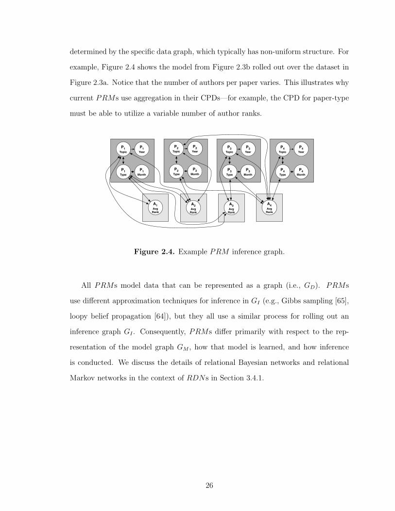
determined by the specific data graph, which typically has non-uniform structure. For

example, Figure 2.4 shows the model from Figure 2.3b rolled out over the dataset in

Figure 2.3a. Notice that the number of authors per paper varies. This illustrates why

current PRMs use aggregation in their CPDs—for example, the CPD for paper-type

must be able to utilize a variable number of author ranks.

P3Month

P3Type

P3Topic

P3Year

P1Month

P1Type

P1Topic

P1Year

A1Avg

Rank

P2Month

P2Type

P2Topic

P2Year

A2Avg

Rank

A3Avg

Rank

A4Avg

Rank

P4Month

P4Type

P4Topic

P4Year

Figure 2.4. Example PRM inference graph.

All PRMs model data that can be represented as a graph (i.e., GD). PRMs

use different approximation techniques for inference in GI (e.g., Gibbs sampling [65],

loopy belief propagation [64]), but they all use a similar process for rolling out an

inference graph GI . Consequently, PRMs differ primarily with respect to the rep-

resentation of the model graph GM , how that model is learned, and how inference

is conducted. We discuss the details of relational Bayesian networks and relational

Markov networks in the context of RDNs in Section 3.4.1.

26

CHAPTER 3

RELATIONAL DEPENDENCY NETWORKS

Joint relational models are able to exploit autocorrelation by estimating a joint

probability distribution over an entire relational dataset and collectively inferring

the labels of related instances. Recent research has produced several novel PRMs

for estimating joint probability distributions for relational data that consist of non-

independent and heterogeneous instances [29, 85, 18, 51, 89]. PRMs extend tradi-

tional graphical models such as Bayesian networks to relational domains, removing

the assumption of i.i.d. instances that underlies propositional learning techniques.

PRMs have been successfully evaluated in several domains, including the World

Wide Web, genomic data, and scientific literature.

Directed PRMs, such as relational Bayesian networks (RBNs) [29], can model

autocorrelation dependencies if they are structured in a manner that respects the

acyclicity constraint of the model. While domain knowledge can sometimes be used

to structure the autocorrelation dependencies in an acyclic manner, often an acyclic

ordering is unknown or does not exist. For example, in genetic pedigree analysis

there is autocorrelation among the genes of relatives [52]. In this domain, the casual

relationship is from ancestor to descendent so we can use the temporal parent-child

relationship to structure the dependencies in an acyclic manner (i.e., parents’ genes

will never be influenced by the genes of their children). However, given a set of

hyperlinked web pages, there is little information to use to determine the causal

direction of the dependency between their topics. In this case, we can only represent

an (undirected) correlation between the topics of two pages, not a (directed) causal

27

relationship. The acyclicity constraint of directed PRMs precludes the learning of

arbitrary autocorrelation dependencies and thus severely limits the applicability of

these models in relational domains.

Undirected PRMs, such as relational Markov networks (RMNs) [89], can repre-

sent arbitrary forms of autocorrelation. However, research on these models focused

primarily on parameter estimation and inference procedures. Current implementa-

tions of RMNs do not select features—model structure must be pre-specified by the

user. While, in principle, it is possible for RMN techniques to learn cyclic autocorre-

lation dependencies, inefficient parameter estimation makes this difficult in practice.

Because parameter estimation requires multiple rounds of inference over the entire

dataset, it is impractical to incorporate it as a subcomponent of feature selection.

Recent work on conditional random fields for sequence analysis includes a feature

selection algorithm [58] that could be extended for RMNs. However, the algorithm

abandons estimation of the full joint distribution during the inner loop of feature se-

lection and uses an approximation instead, which makes the approach tractable but

removes some of the advantages of reasoning with the full joint distribution.

In this chapter, we describe relational dependency networks (RDNs), an extension

of dependency networks [33] for relational data. RDNs can represent the cyclic de-

pendencies required to express and exploit autocorrelation during collective inference.

In this regard, they share certain advantages of RMNs and other undirected models

of relational data [9, 18, 83]. To our knowledge, RDNs are the first PRM capable

of learning cyclic autocorrelation dependencies. RDNs also offer a relatively simple

method for structure learning and parameter estimation, which results in models that

are easier to understand and interpret. In this regard, they share certain advantages

of RBNs and other directed models [85, 34]. The primary distinction between RDNs

and other existing PRMs is that RDNs are an approximate model. RDNs approx-

imate the full joint distribution and thus are not guaranteed to specify a consistent

28

probability distribution, where each CPD can be derived from the joint distribution

using the rules of probability.1 The quality of the approximation will be determined

by the data available for learning—if the models are learned from large datasets,

and combined with Monte Carlo inference techniques, the approximation should be

sufficiently accurate.

We start by reviewing the details of dependency networks for propositional data.

Then we discuss the specifics of RDN learning and inference procedures. We evaluate

RDN learning and inference on synthetic datasets, showing that RDN learning is ac-

curate for large to moderate-size datasets and that RDN inference is comparable, or

superior, to RMN inference over a range of data conditions. In addition, we evaluate

RDNs on five real-world datasets, presenting learned RDNs for subjective evalua-

tion. Of particular note, all the real-world datasets exhibit multiple autocorrelation

dependencies that were automatically discovered by the RDN learning algorithm.

We evaluate the learned models in a prediction context, where only a single attribute

is unobserved, and show that the models outperform conventional conditional models

on all five tasks. Finally, we discuss related work and conclude.

3.1 Dependency Networks

Graphical models represent a joint distribution over a set of variables. The pri-

mary distinction between Bayesian networks, Markov networks, and dependency net-

works (DNs) is that dependency networks are an approximate representation. DNs

approximate the joint distribution with a set of conditional probability distributions

(CPDs) that are learned independently. This approach to learning results in sig-

nificant efficiency gains over models that estimate the joint distribution explicitly.

However, because the CPDs are learned independently, DNs are not guaranteed to

1In this work, we use the term consistent to refer to the consistency of the individual CPDs (asHeckerman et al. [33]), rather than the asymptotic properties of a statistical estimator.

29

specify a consistent joint distribution from which each CPD can be derived using the

rules of probability. This limits the applicability of exact inference techniques. In

addition, the correlational DN representation precludes DNs from being used to in-

fer causal relationships. Nevertheless, DNs can encode predictive relationships (i.e.,

dependence and independence) and Gibbs sampling inference techniques (e.g., [65])

can be used to recover a full joint distribution, regardless of the consistency of the

local CPDs. We begin by reviewing traditional graphical models and then outline the

details of dependency networks in this context.

Consider the set of random variables X = (X1, ..., Xn) over which we would like

to model the joint distribution p(x) = p(x1, ..., xn). We use upper case letters to refer

to random variables and lower case letters to refer to an assignment of values to the

variables.

A Bayesian network for X uses a directed acyclic graph G = (V, E) and a set

of conditional probability distributions P to represent the joint distribution over X.

Each node v ∈ V corresponds to an Xi ∈ X. The edges of the graph encode statistical

dependencies among the variables and can be used to infer conditional independence

among variables using notions of d-separation. The parents of node Xi, denoted

PAi, are the set of vj ∈ V such that (vj, vi) ∈ E. The set P contains a conditional

probability distribution for each variable given its parents, p(xi|pai). The acyclicity

constraint on G ensures that the CPDs in P factor the joint distribution into the

formula below. A directed graph is acyclic if there is no directed path that starts

and ends at the same variable. More specifically, there can be no self-loops from a

variable to itself. Given (G, P ), the joint probability for a set of values x is computed

with the formula:

p(x) =n∏

i=1

p(xi|pai)

A Markov network for X uses an undirected graph U = (V, E) and a set of poten-

tial functions Φ to represent the joint distribution over X. Again, each node v ∈ V

30

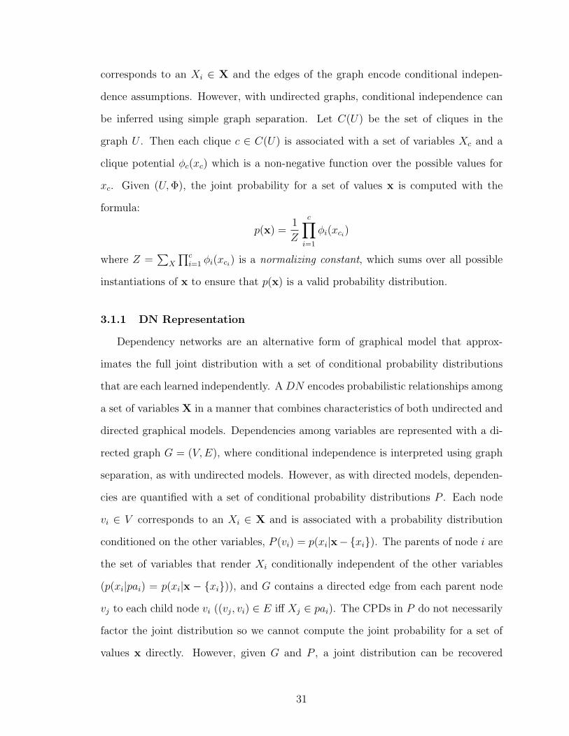
corresponds to an Xi ∈ X and the edges of the graph encode conditional indepen-

dence assumptions. However, with undirected graphs, conditional independence can

be inferred using simple graph separation. Let C(U) be the set of cliques in the

graph U . Then each clique c ∈ C(U) is associated with a set of variables Xc and a

clique potential φc(xc) which is a non-negative function over the possible values for

xc. Given (U, Φ), the joint probability for a set of values x is computed with the

formula:

p(x) =1

Z

c∏i=1

φi(xci)

where Z =∑

X

∏ci=1 φi(xci

) is a normalizing constant, which sums over all possible

instantiations of x to ensure that p(x) is a valid probability distribution.

3.1.1 DN Representation

Dependency networks are an alternative form of graphical model that approx-

imates the full joint distribution with a set of conditional probability distributions

that are each learned independently. A DN encodes probabilistic relationships among

a set of variables X in a manner that combines characteristics of both undirected and

directed graphical models. Dependencies among variables are represented with a di-

rected graph G = (V, E), where conditional independence is interpreted using graph

separation, as with undirected models. However, as with directed models, dependen-

cies are quantified with a set of conditional probability distributions P . Each node

vi ∈ V corresponds to an Xi ∈ X and is associated with a probability distribution

conditioned on the other variables, P (vi) = p(xi|x−xi). The parents of node i are

the set of variables that render Xi conditionally independent of the other variables

(p(xi|pai) = p(xi|x − xi)), and G contains a directed edge from each parent node

vj to each child node vi ((vj, vi) ∈ E iff Xj ∈ pai). The CPDs in P do not necessarily

factor the joint distribution so we cannot compute the joint probability for a set of

values x directly. However, given G and P , a joint distribution can be recovered

31

through Gibbs sampling (see Section 3.2.3 for details). From the joint distribution,

we can extract any probabilities of interest.

For example, the DN in Figure 3.1 models the set of variables: X = X1, X2, X3,

X4, X5. Each node is conditionally independent of the other nodes in the graph

given its immediate neighbors (e.g., X1 is conditionally independent of X2, X4 given

X3, X5). Each node contains a CPD, which specifies a probability distribution over

its possible values, given the values of its parents.

X1

X3

X2

X4X5 p(X4 | X2,X3)

p(X2 | X3,X4)

p(X5 | X1)

p(X1 | X3,X5)

p(X3 | X1,X2,X4)

Figure 3.1. Example DN .

3.1.2 DN Learning

Both the structure and parameters of DNs are determined through learning the lo-

cal CPDs. The DN learning algorithm learns a separate distribution for each variable

Xi, conditioned on the other variables in the data (i.e., X− Xi). Any conditional

learner can be used for this task (e.g., logistic regression, decision trees). The CPD is

included in the model as P (vi) and the variables selected by the conditional learner

form the parents of Xi (e.g., if p(xi|x−xi) = αxj +βxk then PAi = xj, xk). The

parents are then reflected in the edges of G appropriately. If the conditional learner

is not selective (i.e., the algorithm does not select a subset of the features), the DN

will be fully connected (i.e., PAi = x−xi). In order to build understandable DNs,

32

it is desirable to use a selective learner that will learn CPDs that use a subset of all

available variables.

3.1.3 DN Inference

Although the DN approach to structure learning is simple and efficient, it can

result in an inconsistent network, both structurally and numerically. In other words,

there may be no joint distribution from which each of the CPDs can be obtained using

the rules of probability. Learning the CPDs independently with a selective conditional

learner can result in a network that contains a directed edge from Xi to Xj, but not

from Xj to Xi. This is a structural inconsistency—Xi and Xj are dependent but Xj

is not represented in the CPD for Xi. In addition, learning the CPDs independently

from finite samples may result in numerical inconsistencies in the parameter estimates.

If this is the case, the joint distribution derived numerically from the CPDs will not

sum to one. However, when a DN is inconsistent, approximate inference techniques

can still be used to estimate a full joint distribution and extract probabilities of

interest. Gibbs sampling can be used to recover a full joint distribution, regardless of

the consistency of the local CPDs, provided that each Xi is discrete and its CPD is

positive [33]. In practice, Heckerman et al. [33] show that DNs are nearly consistent

if learned from large datasets because the data serve a coordinating function to ensure

some degree of consistency among the CPDs.

3.2 Relational Dependency Networks

Several characteristics of DNs are particularly desirable for modeling relational

data. First, learning a collection of conditional models offers significant efficiency

gains over learning a full joint model. This is generally true, but it is even more

pertinent to relational settings where the feature space is very large. Second, networks

that are easy to interpret and understand aid analysts’ assessment of the utility

33

of the relational information. Third, the ability to represent cycles in a network

facilitates reasoning with autocorrelation, a common characteristic of relational data.

In addition, whereas the need for approximate inference is a disadvantage of DNs for

propositional data, due to the complexity of relational model graphs in practice, all

PRMs use approximate inference.

Relational dependency networks extend DNs to work with relational data in much

the same way that RBNs extend Bayesian networks and RMNs extend Markov

networks. We describe the characteristics of RDNs within the PRM framework

described in Section 2.5.

3.2.1 RDN Representation

Relational dependency networks encode probabilistic relationships in a similar

manner to DNs, extending the representation to a relational setting. RDNs define

a generic dependency structure at the level of item types, using a directed model

graph GM and a set of conditional probability distributions P . Each node vi ∈ VM

corresponds to an X tk ∈ Xt, t ∈ T . The set of variables Xt

k = (X tik : (vi ∈ VD ∨ ei ∈

ED)∧T (i) = t) is tied together and modeled as a single variable X tk, with an associated

conditional distribution p(xtk | paxt

k).

Figure 2.3b illustrates an example RDN model graph for the data graph in Fig-

ure 2.3a. The graphical representation illustrates the qualitative component (GD) of

the RDN—it does not depict the quantitative component (P ) of the model, which

consists of CPDs that use aggregation functions. Although conditional independence

is inferred using an undirected view of the graph, directed edges are useful for rep-

resenting the set of variables in each CPD. For example, in Figure 2.3b the CPD for

year contains topic but the CPD for topic does not contain year. This represents

inconsistencies that may result from the RDN learning technique.

34

A consistent RDN specifies a joint probability distribution p(x) over the attribute

values of a relational dataset from which each CPD ∈ P can be derived using the

rules of probability. There is a direct correspondence between consistent RDNs and

relational Markov networks. It is similar to the correspondence between consistent

DNs and Markov networks [33], but the correspondence is defined with respect to

the template model graphs GM and UM .

Theorem 1. The set of positive distributions that can be encoded by a consistent

RDN (GM , P ) is equal to the set of positive distributions that can be encoded by an

RMN(UM , Φ) provided (1) GM = UM , and (2) P and Φ use the same aggregations

functions.

Proof. Let p be a positive distribution defined by an RMN (UM , Φ) for GD. First,

we construct a Markov network with tied clique potentials by rolling out the RMN

inference graph UI over the data graph GD. By Theorem 1 of [33], which uses the

Hammersley-Clifford theorem [3], there is a corresponding dependency network that

represents the same distribution p as the Markov network UI . Since the conditional

probability distribution for each occurrence of an attribute k of a given type t (i.e.,

∀i (vi ∈ VD ∨ ei ∈ ED) ∧ T (i) = t p(xtik|x)) is derived from the Markov network, we

know that the resulting CPDs will be identical—the nodes adjacent to each occurrence

are equivalent by definition, thus by the global Markov property the derived CPDs

will be identical. From this dependency network we can construct a consistent RDN

(GM , P ) by first setting GM = UM . Next, we compute from UI the CPDs for the

attributes of each item type: p(xtk|x−xt

k) for t ∈ T,X tk ∈ Xt. To derive the CPDs

for P , the CPDs must utilize the same aggregation functions as the potentials in Φ.

Since the adjacencies in the RDN model graph are the same as those in the RMN

model graph, and there is a correspondence between the rolled out DN and MN, the

distribution encoded by the RDN is p.

35

Next let p be a positive distribution defined by an RDN (GM , P ) for GD. First,

we construct a dependency network with tied CPDs by rolling out the RDN infer-

ence graph GI over the data graph GD. Again, by Theorem 1 of [33], there is a

corresponding Markov network that represents the same distribution p as the depen-

dency network GI . Of the valid Markov networks representing p, there will exist a

network where the potentials are tied across occurrences of the same clique template

(i.e., ∀ci ∈ C φC(xC)). This follows from the first part of the proof, which shows

that each RMN with tied clique potentials can be transformed to an RDN with tied

CPDs. From this Markov network we can construct an RMN (UM , Φ) by setting

UM = GM and grouping the set of clique template potentials in Φ. Since the adjacen-

cies in the RMN model graph are the same as those in the RDN model graph, and

since there is a correspondence between the rolled out MN and DN , the distribution

encoded by the RMN is p.

This proof shows an exact correspondence between consistent RDNs and RMNs.

We cannot show the same correspondence for general RDNs. However, we show in

Section 3.2.3 that Gibbs sampling can be used to extract a unique joint distribution,

regardless of the consistency of the model.

3.2.2 RDN Learning

Learning a PRM consists of two tasks: learning the dependency structure among

the attributes of each object type, and estimating the parameters of the local prob-

ability models for an attribute given its parents. Relatively efficient techniques exist

for learning both the structure and parameters of RBNs. However, these techniques

exploit the requirement that the CPDs factor the full distribution—a requirement

that imposes acyclicity constraints on the model and precludes the learning of ar-

bitrary autocorrelation dependencies. On the other hand, although, in principle, it

is possible for RMN techniques to learn cyclic autocorrelation dependencies, inef-

36

ficiencies due to calculating the normalizing constant Z in undirected models make

this difficult in practice. Calculation of Z requires a summation over all possible

states x. When modeling the joint distribution of propositional data, the number

of states is exponential in the number of attributes (i.e., O(2m)). When modeling

the joint distribution of relational data, the number of states is exponential in the

number of attributes and the number of instances. If there are N objects, each with

m attributes, then the total number of states is O(2Nm). For any reasonable-size

dataset, a single calculation of Z is an enormous computational burden. Feature se-

lection generally requires repeated parameter estimation while measuring the change

in likelihood affected by each attribute, which would require recalculation of Z on

each iteration.

The RDN learning algorithm uses a more efficient alternative—estimating the

set of conditional distributions independently rather than jointly. This approach is

based on pseudolikelihood techniques [4], which were developed for modeling spatial

datasets with similar autocorrelation dependencies. The pseudolikelihood for data

graph GD is computed as a product over the item types T , the attributes of that type

X t, and the items of that type v, e:

PL(GD; θ) =∏t∈T

∏Xt

i∈Xt

∏v:T (v)=t

p(xtvi|paxt

vi; θ)

∏e:T (e)=t

p(xtei|paxt

ei; θ) (3.1)

On the surface, Equation 3.1 may appear similar to a likelihood that specifies a

joint distribution of an RBN . However, the CPDs in the RDN pseudolikelihood

are not required to factor the joint distribution of GD. More specifically, when we

consider the variable X tvi, we condition on the values of the parents PAXt

viregardless

of whether the estimation of CPDs for variables in PAXtvi

was conditioned on X tvi.

The parents of X tvi may include other variables on the same item (e.g., X t

vi′ such that

i′ 6= i), the same variable on related items (e.g., X tv′i such that v′ 6= v), or other

variables on related items (e.g., X t′

v′i′ such that v′ 6= v and i′ 6= i).

37

Pseudolikelihood estimation avoids the complexities of estimating Z and the re-

quirement of acyclicity. Instead of optimizing the log-likelihood of the full joint dis-

tribution, we optimize the pseudo-loglikelihood. The contribution for each variable

is conditioned on all other attribute values in the data, thus we can maximize the

pseudo-loglikelihood for each variable independently:

log PL(GD; θ) =∑t∈T

∑Xt

i∈Xt

∑v:T (v)=t

log p(xtvi|paxt

vi; θ) +

∑e:T (e)=t

log p(xtei|paxt

ei; θ)

In addition, this approach can utilize existing techniques for learning conditional

probability distributions of relational data such as first-order Bayesian classifiers [24],

structural logistic regression [82], or ACORA [79].

Maximizing the pseudolikelihood function gives the maximum pseudolikelihood

estimate (MPLE) of θ. To estimate the parameters we need to solve the following

pseudolikelihood equation:

∂

∂θPL(GD; θ) = 0 (3.2)

With this approach, we lose the asymptotic efficiency properties of maximum like-

lihood estimators. However, under some general conditions the asymptotic properties

of the MPLE can be established. In particular, in the limit as sample size grows, the

MPLE will be an unbiased estimate of the true parameter θ0 and it will be normally

distributed. Geman and Graffine [28] established the first proof of the properties of

maximum pseudolikelihood estimators of fully observed data. Gidas [31] gives an al-

ternative proof and Comets [10] establishes a more general proof that does not require

finite state space x or stationarity of the true distribution Pθ0 .

Theorem 2. Assuming the following regularity conditions2 are satisfied for an RDN :

1. The model is identifiable, that is if θ 6= θ′, then PL(GD; θ) 6= PL(GD; θ′).

2These are the standard regularity conditions (e.g., [8]) used to prove asymptotic properties ofestimators, which are usually satisfied in most reasonable problems.

38

2. The distributions PL(GD; θ) have common support and are differentiable with

respect to θ.

3. The parameter space Ω contains an open set ω of which the true parameter θ0

is an interior point.

In addition, assuming the pseudolikelihood equation (3.2) has a unique solution in ω

almost surely as |GD| → ∞, then, provided that GD is of bounded degree, the MPLE

θ converges in probability to the true value θ0 as |GD| → ∞.

Proof. Provided the size of the RDN model graph does not grow as the size of the

dataset grows (i.e., |P | remains constant as |GD| → ∞) and GD is of bounded degree,

then previous proofs apply. We provide the intuition for the proof here and refer the

reader to [10, 93, 53] for details. Let θ be the maximum pseudolikelihood estimate

that maximizes PL(GD; θ). As |GD| → ∞, the data will consist of all possible data

configurations for each CPD ∈ P (assuming bounded degree structure in GD). As

such, the pseudolikelihood function will converge to its expectation, PL(GD; θ) →

E(PL(GD; θ)). The expectation is maximized by the true parameter θ0 because the

expectation is taken with respect to all possible data configurations. Therefore as

|GD| → ∞, the MPLE converges to the true parameter (i.e., θ − θ0 → 0).

The RDN learning algorithm is similar to the DN learning algorithm, except we

use a relational probability estimation algorithm to learn the set of conditional mod-

els, maximizing pseudolikelihood for each variable separately. The algorithm input

consists of: (1) GD: a relational data graph, (2) R: a conditional relational learner,

and (3) Qt: a set of queries3 that specify the relational neighborhood considered in

R for each type T .

3Our implementation utilizes a set of user-specified queries to limit the search space consideredduring learning. However, a simple depth limit (e.g., ≤ 2 links away in the data graph) can be usedto limit the search space as well.

39

Table 1 outlines the learning algorithm in pseudocode. It cycles over each attribute

of each item type and learns a separate CPD, conditioned on the other values in the

training data. We discuss details of the subcomponents (querying and relational

learners) in the sections below.

Quantifying the asymptotic complexity of PRM learners is difficult due to the

use of heuristic search and numerical optimization techniques. The asymptotic com-

plexity of RDN learning is O(|X| · |PAX | ·N), where |X| is the number of CPDs to be

estimated, |PAX | is the number of attributes, and N is the number of instances, used

to estimate the CPD for X.4 RBN learning requires multiple rounds of parameter

estimation during the algorithm’s heuristic search through the model space, and each

round of parameter estimation has the same complexity as RDN learning, thus RBN

learning will generally require more time. For RMN learning, there is no closed-form

parameter estimation technique. Instead, the models are trained using conjugate gra-

dient, where each iteration requires approximate inference over the unrolled Markov

network. In general this RMN nested loop of optimization and approximation will

require more time to learn than an RBN [89]. Therefore, given equivalent search

spaces, RMN learning is generally more complex than RBN learning, and RBN

learning is generally more complex than RDN learning.

3.2.2.1 Conditional Relational Learners

The conditional relational learner R is used for both parameter estimation and

structure learning in RDNs. The variables selected by R are reflected in the edges of

GM appropriately. If R selects all of the available attributes, the RDN will be fully

connected.

4This assumes the complexity of the relational learner R is O(|PAX | · N), which is true for theconditional relational learners considered in this work (i.e., RBCs and RPT s).

40

Learn RDN (GD, R,Qt):P ← ∅For each t ∈ T :

For each X tk ∈ Xt:

Use R to learn a CPD for X tk given the attributes in the relational

neighborhood defined by Qt.P ← P ∪ CPDXt

k

Use P to form GM .

Table 3.1. RDN learning algorithm.

In principle, any conditional relational learner can be used as a subcomponent to

learn the individual CPDs provided that it can closely approximate CPDs consistent

with the joint distribution. In this chapter, we discuss the use of two different condi-

tional models—relational Bayesian classifiers (RBCs) [76] and relational probability

trees (RPT s) [75].

Relational Bayesian Classifiers

RBCs extend naive Bayesian classifiers to a relational setting. RBCs treat heteroge-

neous relational subgraphs as a homogenous set of attribute multisets. For example,

when considering the references of a single paper, the publication dates of those ref-

erences form multisets of varying size (e.g., 1995, 1995, 1996, 1975, 1986, 1998,

1998). The RBC assumes each value of a multiset is independently drawn from the

same multinomial distribution.5 This approach is designed to mirror the indepen-

dence assumption of the naive Bayesian classifier. In addition to the conventional

assumption of attribute independence, the RBC also assumes attribute value inde-

pendence within each multiset.

5Alternative constructions are possible but prior work [76] has shown this approach achievessuperior performance over a wide range of conditions.

41

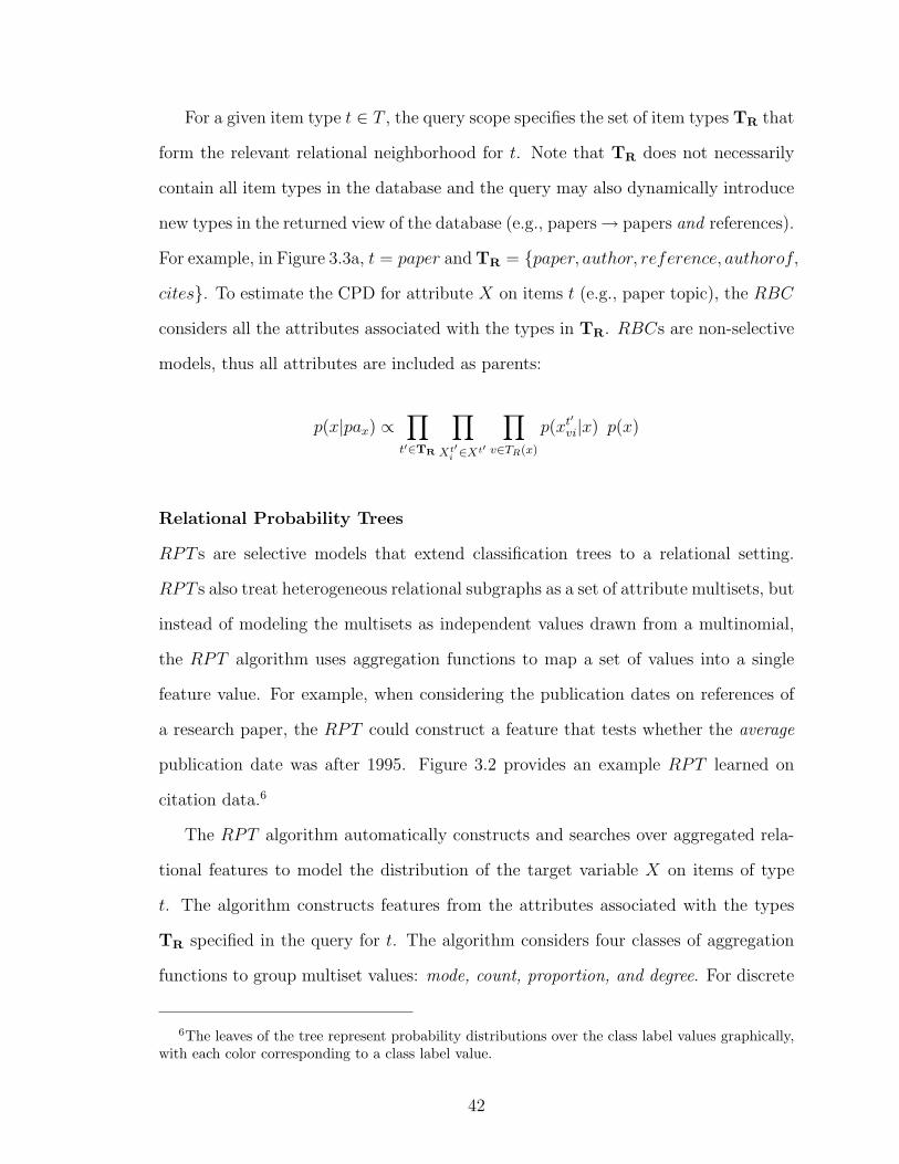
For a given item type t ∈ T , the query scope specifies the set of item types TR that

form the relevant relational neighborhood for t. Note that TR does not necessarily

contain all item types in the database and the query may also dynamically introduce

new types in the returned view of the database (e.g., papers→ papers and references).

For example, in Figure 3.3a, t = paper and TR = paper, author, reference, authorof,

cites. To estimate the CPD for attribute X on items t (e.g., paper topic), the RBC

considers all the attributes associated with the types in TR. RBCs are non-selective

models, thus all attributes are included as parents:

p(x|pax) ∝∏

t′∈TR

∏Xt′

i ∈Xt′

∏v∈TR(x)

p(xt′

vi|x) p(x)

Relational Probability Trees

RPT s are selective models that extend classification trees to a relational setting.

RPT s also treat heterogeneous relational subgraphs as a set of attribute multisets, but

instead of modeling the multisets as independent values drawn from a multinomial,

the RPT algorithm uses aggregation functions to map a set of values into a single

feature value. For example, when considering the publication dates on references of

a research paper, the RPT could construct a feature that tests whether the average

publication date was after 1995. Figure 3.2 provides an example RPT learned on

citation data.6

The RPT algorithm automatically constructs and searches over aggregated rela-

tional features to model the distribution of the target variable X on items of type

t. The algorithm constructs features from the attributes associated with the types

TR specified in the query for t. The algorithm considers four classes of aggregation

functions to group multiset values: mode, count, proportion, and degree. For discrete

6The leaves of the tree represent probability distributions over the class label values graphically,with each color corresponding to a class label value.

42

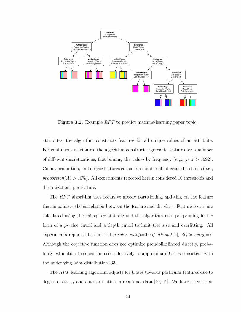
ReferenceMode(Topic=

NeuralNetworks)

AuthorPaperProportion(Topic=

NeuralNetworks)>20%

ReferenceProportion(Topic=Theory)>25%

AuthorPaperProportion(Topic=GeneticAlgs)>45%

AuthorPaperProportion(Topic=ProbMethods)>15%

AuthorPaperProportion(Topic=GeneticAlgs)>45%

AuthorPaperProportion(Topic=CaseBased)>15%

ReferenceMode(Topic=ProbMethods)

ReferenceMode(Topic=GeneticAlgs)

ReferenceMode(Topic=CaseBased)

ReferenceMode(Topic=ReinforceLearn)

Y N

Y Y

Y

Y

N N

N

N

Y N N NY Y

Y

Y Y

N

N N

Figure 3.2. Example RPT to predict machine-learning paper topic.

attributes, the algorithm constructs features for all unique values of an attribute.

For continuous attributes, the algorithm constructs aggregate features for a number

of different discretizations, first binning the values by frequency (e.g., year > 1992).

Count, proportion, and degree features consider a number of different thresholds (e.g.,

proportion(A) > 10%). All experiments reported herein considered 10 thresholds and

discretizations per feature.

The RPT algorithm uses recursive greedy partitioning, splitting on the feature

that maximizes the correlation between the feature and the class. Feature scores are

calculated using the chi-square statistic and the algorithm uses pre-pruning in the

form of a p-value cutoff and a depth cutoff to limit tree size and overfitting. All

experiments reported herein used p-value cutoff=0.05/|attributes|, depth cutoff=7.

Although the objective function does not optimize pseudolikelihood directly, proba-

bility estimation trees can be used effectively to approximate CPDs consistent with

the underlying joint distribution [33].

The RPT learning algorithm adjusts for biases towards particular features due to

degree disparity and autocorrelation in relational data [40, 41]. We have shown that

43

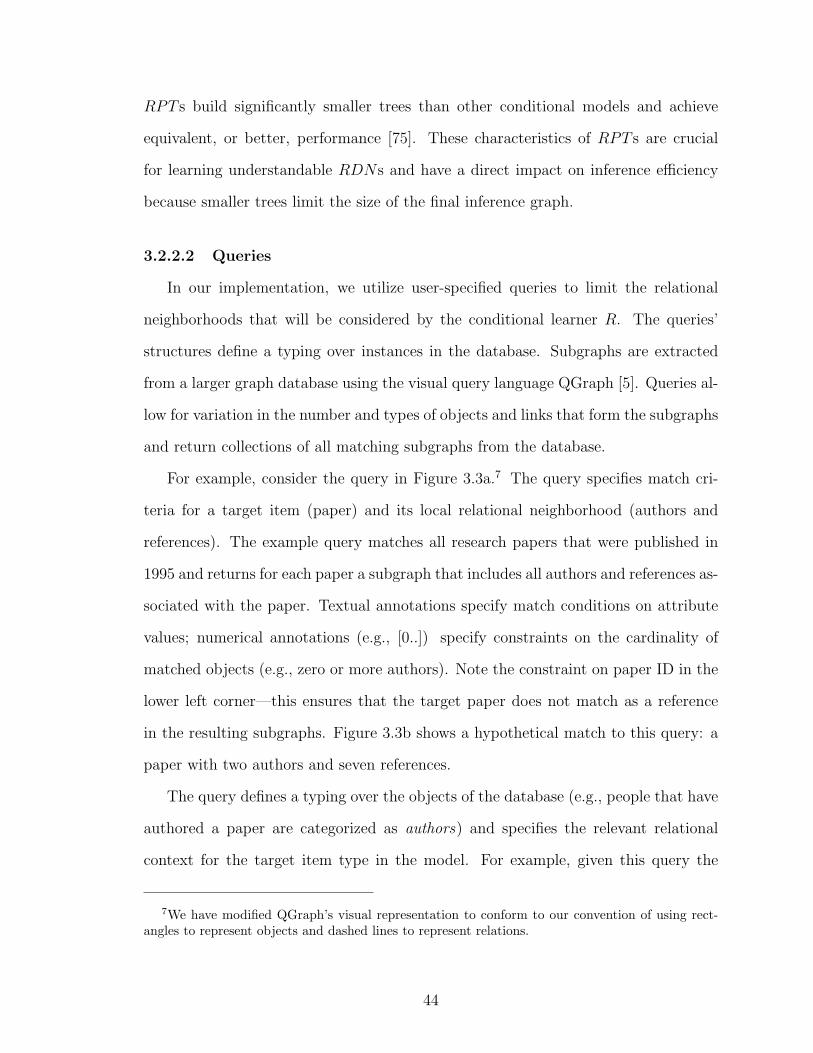
RPT s build significantly smaller trees than other conditional models and achieve

equivalent, or better, performance [75]. These characteristics of RPT s are crucial

for learning understandable RDNs and have a direct impact on inference efficiency

because smaller trees limit the size of the final inference graph.

3.2.2.2 Queries

In our implementation, we utilize user-specified queries to limit the relational

neighborhoods that will be considered by the conditional learner R. The queries’

structures define a typing over instances in the database. Subgraphs are extracted

from a larger graph database using the visual query language QGraph [5]. Queries al-

low for variation in the number and types of objects and links that form the subgraphs

and return collections of all matching subgraphs from the database.

For example, consider the query in Figure 3.3a.7 The query specifies match cri-

teria for a target item (paper) and its local relational neighborhood (authors and

references). The example query matches all research papers that were published in

1995 and returns for each paper a subgraph that includes all authors and references as-

sociated with the paper. Textual annotations specify match conditions on attribute

values; numerical annotations (e.g., [0..]) specify constraints on the cardinality of

matched objects (e.g., zero or more authors). Note the constraint on paper ID in the

lower left corner—this ensures that the target paper does not match as a reference

in the resulting subgraphs. Figure 3.3b shows a hypothetical match to this query: a

paper with two authors and seven references.

The query defines a typing over the objects of the database (e.g., people that have

authored a paper are categorized as authors) and specifies the relevant relational

context for the target item type in the model. For example, given this query the

7We have modified QGraph’s visual representation to conform to our convention of using rect-angles to represent objects and dashed lines to represent relations.

44

Paper

Author

Refer-ence

Refer-ence

Refer-ence

Refer-ence

Refer-ence

Refer-ence

Refer-enceAuthor

Paper

Author

Linktype=AuthorOf

Refer-ence

Linktype=CitesAND(Objecttype=Paper,

Year=1995)

Objecttype=Person

Objecttype=Paper[0..]

[0..]

(a) (b)

Paper.ID!=Reference.ID

Figure 3.3. (a) Example QGraph query, and (b) matching subgraph.

learner R would model the distribution of a paper’s attributes given the attributes of

the paper itself and the attributes of its related authors and references. The queries

are a means of restricting model search. Instead of setting a simple depth limit on

the extent of the search, the analyst has a more flexible means with which to limit

the search (e.g., we can consider other papers written by the paper’s authors but not

other authors of the paper’s references, both at the same depth).

3.2.3 RDN Inference

The RDN inference graph GI is potentially much larger than the original data

graph. To model the full joint distribution there must be a separate node (and CPD)

for each attribute value in GD. To construct GI , the set of template CPDs in P is

rolled out over the test-set data graph. Each item-attribute pair gets a separate, local

copy of the appropriate CPD. Consequently, the total number of nodes in the inference

graph will be∑

v∈VD|XT(v)|+

∑e∈ED

|XT(e)|. Roll out facilitates generalization across

data graphs of varying size—we can learn the CPD templates from one data graph

and apply the model to a second data graph with a different number of objects by

rolling out more CPD copies. This approach is analogous to other graphical models

that tie distributions across the network and roll out copies of model templates (e.g.,

hidden Markov models, conditional random fields [51]).

45

We use randomly ordered Gibbs samplers (e.g., [65]) for inference in RDNs. This

refers to a procedure where a random ordering of the variables is selected; each vari-

able is initialized to an arbitrary value; and then each variable is visited (repeatedly)

in order, where its value is resampled according to its conditional distribution. Gibbs

sampling can be used to extract a unique joint distribution, regardless of the consis-

tency of the model.

Theorem 3. The procedure of a randomly ordered Gibbs sampler applied to an RDN

(G, P ), where each Xi is discrete and each local distribution in P is positive, defines a

Markov chain with a unique stationary joint distribution π for X that can be reached

from any initial state of the chain.

Proof. The proof that Gibbs sampling can be used to estimate the joint distribution

of a dependency network [33] applies to rolled out RDNs as well. We restate the

proof here for completeness.

Let xt be the sample of x after the tth iteration of the Gibbs sampler. The sequence

x1,x2, ... can be viewed as samples drawn from a homogeneous Markov chain with

transition matrix P, where Pij = p(xt+1 = j|xt = i). The matrix P is the product

P1 · P2 · ... · Pn, where Pk is the local transition matrix describing the resampling

of Xk according to the local distribution of p(xk|pak). The positivity of the local

distributions guarantees the positivity of P. The positivity of P in turn guarantees

that the Markov chain is irreducible and aperiodic. Consequently there exists a unique

joint distribution that is stationary with respect to P, and this stationary distribution

can be reached from any starting point.

This shows that an ordered Gibbs sampling procedure can be used with an RDN

to recover samples from a unique stationary distribution π, but how close will this

distribution be to the true distribution π? Small perturbations in the local CPDs

could propagate in the Gibbs sampling procedure to produce large deviations in the

46

stationary distribution. Heckerman et al. [33] provide some initial theoretical analysis

that suggests that Markov chains with good convergence properties will be insensitive

to deviations in the transition matrix. This implies that when Gibbs sampling is

effective (i.e., converges), then π will be close to π and the RDN will be a close

approximation to the full joint distribution.

Table 2 outlines the inference algorithm. To estimate a joint distribution, we start

by rolling out the model GM onto the target dataset GD and forming the inference

graph GI . The values of all unobserved variables are initialized to values drawn from

their prior distributions. Gibbs sampling then iteratively relabels each unobserved

variable by drawing from its local conditional distribution, given the current state of

the rest of the graph. After a sufficient number of iterations (burn in), the values

will be drawn from a stationary distribution and we can use the samples to estimate

probabilities of interest.

For prediction tasks, we are often interested in the marginal probabilities associ-

ated with a single variable X (e.g., paper topic). Although Gibbs sampling may be

a relatively inefficient approach to estimating the probability associated with a joint

assignment of values of X (e.g., when |X| is large), it is often reasonably fast to use

Gibbs sampling to estimate the marginal probabilities for each X.

There are many implementation issues that can improve the estimates obtained

from a Gibbs sampling chain, such as length of burn-in and number of samples. For

the experiments reported in this work, we used fixed-length chains of 2000 samples

(each iteration re-labels every value sequentially) with burn-in set at 100. Empiri-

cal inspection indicated that the majority of chains had converged by 500 samples.

Section 3.3.1 includes convergence graphs for synthetic data experiments.

47

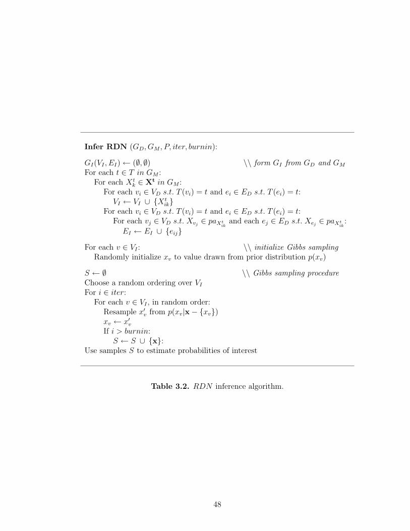
Infer RDN (GD, GM , P, iter, burnin):

GI(VI , EI)← (∅, ∅) \\ form GI from GD and GM

For each t ∈ T in GM :For each X t

k ∈ Xt in GM :For each vi ∈ VD s.t. T (vi) = t and ei ∈ ED s.t. T (ei) = t:

VI ← VI ∪ X tik

For each vi ∈ VD s.t. T (vi) = t and ei ∈ ED s.t. T (ei) = t:For each vj ∈ VD s.t. Xvj

∈ paXtik

and each ej ∈ ED s.t. Xej∈ paXt

ik:

EI ← EI ∪ eij

For each v ∈ VI : \\ initialize Gibbs samplingRandomly initialize xv to value drawn from prior distribution p(xv)

S ← ∅ \\ Gibbs sampling procedureChoose a random ordering over VI

For i ∈ iter:For each v ∈ VI , in random order:

Resample x′v from p(xv|x− xv)

xv ← x′v

If i > burnin:S ← S ∪ x:

Use samples S to estimate probabilities of interest

Table 3.2. RDN inference algorithm.

48

3.3 Experimental Evaluation

The experiments in this section demonstrate the utility of RDNs as a joint model

of relational data. First, we use synthetic data to assess the impact of training-set size

and autocorrelation on RDN learning and inference, showing that accurate models

can be learned with reasonable dataset sizes and that RDN learning is robust to

varying levels of autocorrelation. In addition, to assess the quality of the RDN ap-

proximation for inference, we compare RDNs to RMNs, showing that RDNs achieve

equivalent or better performance over a range of datasets. Next, we learn RDNs of

five real-world datasets to illustrate the types of domain knowledge that the models

discover automatically. In addition, we evaluate RDNs in a prediction context, where

only a single attribute is unobserved in the test set, and report significant performance

gains compared to two individual models.

3.3.1 Synthetic Data Experiments

To explore the effects of training-set size and autocorrelation on RDN learning

and inference, we generated homogeneous data graphs with an autocorrelated class

label and linkage due to an underlying (hidden) group structure. Each object has

four boolean attributes: X1, X2, X3, and X4. See appendix A.1.1 for a detailed

description of the data generation process.

We compare two different RDNs, learning models with queries that include all

neighbors one link away in the data graph. The RDNRBC uses RBCs for the compo-

nent learner R; the RDNRPT uses RPT s for R. The RPT performs feature selection,

which may result in structural inconsistencies in the learned RDN . The RBC does

not use feature selection so any deviation from the true model is due to parameter

inconsistencies alone. Note that the two models do not consider identical feature

spaces so we can only roughly assess the impact of feature selection by comparing

RDNRBC and RDNRPT results.

49

3.3.1.1 RDN Learning

The first set of synthetic experiments examines the effectiveness of the RDN

learning algorithm. Our theoretical analysis indicates that, in the limit, the true

parameters will maximize the pseudolikelihood function. This implies that the pseu-

dolikelihood function, evaluated at the learned parameters, will be no greater than

the pseudolikelihood of the true model (on average). To evaluate the quality of the

RDN parameter estimates, we calculated the pseudolikelihood of the test-set data

using both the true model (used to generate the data) and the learned models. If

the pseudolikelihood given the learned parameters approaches the pseudolikelihood

given the true parameters, then we can conclude that parameter estimation is suc-

cessful. We also measured the standard error of the pseudolikelihood estimate for a

single test-set using learned models from 10 different training sets. This illustrates

the amount of variance due to parameter estimation.

Figure 3.4 graphs the pseudo-loglikelihood of learned models as a function of

training-set size for three levels of autocorrelation. Training-set size was varied at

the levels 50, 100, 250, 500, 1000, 5000. We varied p(X1|X1R, X2) to generate data

with approximate levels of autocorrelation corresponding to 0.25, 0.50, 0.75. At

each training set size (and autocorrelation level), we generated 10 test sets. For each

test set, we generated 10 training sets and learned RDNs. Using each learned model,

we measured the pseudolikelihood of the test set (size 250) and averaged the results

over the 10 models. We plot the mean pseudolikelihood for both the learned models

and the RDN used for data generation, which we refer to as True Model. The top

row reports experiments with data generated from an RDNRPT where we learned

an RDNRPT . The bottom row reports experiments with data generated from an

RDNRBC , where we learned an RDNRBC .

50

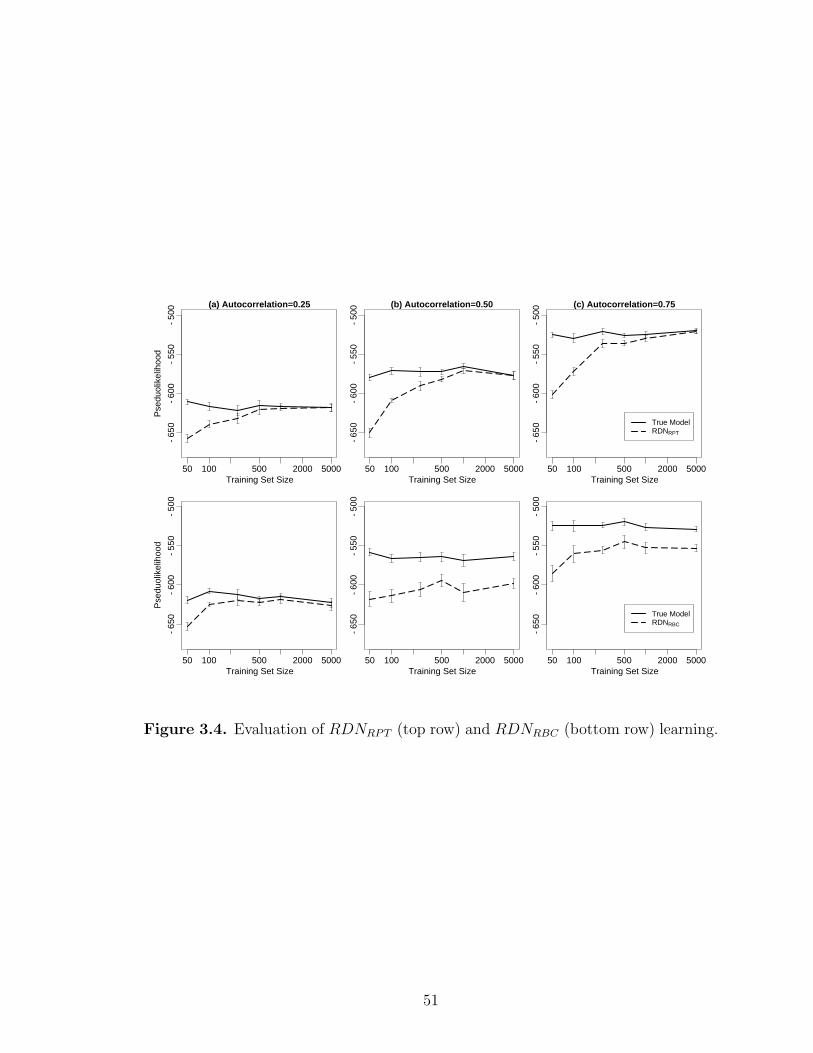
(a) Autocorrelation=0.25

−65

0−

600

−55

0−

500

50 100 500 2000 5000

Pse

duol

ikel

ihoo

d

Training Set Size

(b) Autocorrelation=0.50

−65

0−

600

−55

0−

500

50 100 500 2000 5000Training Set Size

(c) Autocorrelation=0.75

−65

0−

600

−55

0−

500

50 100 500 2000 5000Training Set Size

True ModelRDNRPT

−65

0−

600

−55

0−

500

50 100 500 2000 5000

Pse

duol

ikel

ihoo

d

Training Set Size

−65

0−

600

−55

0−

500

50 100 500 2000 5000Training Set Size

−65

0−

600

−55

0−

500

50 100 500 2000 5000Training Set Size

True ModelRDNRBC

Figure 3.4. Evaluation of RDNRPT (top row) and RDNRBC (bottom row) learning.

51

These experiments show that the learned RDNRPT is a good approximation to

the true model by the time training-set size reaches 500, and that RDNRPT learning

is robust with respect to varying levels of autocorrelation.

There appears to be little difference between the RDNRPT and RDNRBC when

autocorrelation is low, but otherwise the RDNRBC needs significantly more data to

estimate the parameters accurately. One possible source of error is variance due to

lack of selectivity in the RDNRBC(i.e., the model uses all available attributes), which

necessitates the estimation of a greater number of parameters. However, there is little

improvement even when we increase the size of the training sets to 10,000 objects.

Furthermore, the discrepancy between the estimated model and the true model is

greatest when autocorrelation is moderate. This indicates that the inaccuracies may

be due to the naive Bayes independence assumption and its tendency to produce

biased probability estimates [96].

3.3.1.2 RDN Inference

The second set of synthetic experiments evaluates the RDN inference procedure

in a prediction context, where only a single attribute is unobserved in the test set.

We generated data in the manner described above and learned models to predict X1

using the intrinsic attributes of the object (X2, X3, X4) as well as the class label and

the attributes of directly related objects (X1, X2, X3, X4). At each autocorrelation

level, we generated 10 training sets (size 500) to learn the models. For each training

set, we generated 10 test sets (size 250) and used the learned models to infer marginal

probabilities for X1 on the test set instances. To evaluate the predictions, we report

AUC results.8 These experiments used the same levels of autocorrelation outlined

above.

8Squared-loss results are qualitatively similar to the AUC results reported in Figure 3.5.

52

We compare the performance of four types of models. First, we measure the

performance of RPT s and RBCs. These are individual models that represent each

instance independently and do not use the class labels of related instances. Second, we

measure the performance of the two RDNs described above: RDNRBC and RDNRPT .

Third, we measure performance of the two RDNs while allowing the true labels

of related instances to be utilized during inference. This demonstrates the level of

performance possible if the RDNs could infer the true labels of related instances

with perfect accuracy. We refer to these as ceiling models : RDNCeilRBC and RDNCeil

RPT .

Fourth, we measure the performance of two RMNs described below.

The first RMN is non-selective. We construct features from all the attributes

available to the RDNs, defining clique templates for each pairwise combination of

class label value and attribute value. More specifically, the available attributes con-

sist of the intrinsic attributes of objects, and both the class label and attributes of

directly related objects. The second RMN model, which we refer to as RMNSel, is a

hybrid selective model—clique templates are only specified for the set of attributes se-

lected by the RDN during learning. For both models, we used maximum-a-posteriori

parameter estimation to estimate the feature weights, using conjugate gradient with

zero-mean Gaussian priors, and a uniform prior variance of 5.9 For RMN inference,

we used loopy belief propagation [64].

We do not compare directly to RBNs because their acyclicity constraint prevents

them from representing the autocorrelation dependencies in this domain. Instead,

we include the performance of individual models, which also cannot represent the

autocorrelation of X1. Although RBNs and individual models cannot represent the

autocorrelation directly, they can exploit the autocorrelation indirectly by using the

observed attributes of related instances. For example, if there is a correlation be-

9We experimented with a range of priors; this parameter setting produced the best empiricalresults.

53

tween the words on a webpage and its topic, and the topics of hyperlinked pages

are autocorrelated, then the models can exploit autocorrelation dependencies indi-

rectly by modeling the contents of a webpage’s neighboring pages. Recent work has

shown that collective models (e.g., RDNs) are a low-variance means of reducing bias

through direct modeling of the autocorrelation dependencies [42]. Models that ex-

ploit autocorrelation dependencies indirectly by modeling the observed attributes of

related instances, experience a dramatic increase in variance as the number of ob-

served attributes increases.

During inference we varied the number of known class labels in the test set, mea-

suring performance on the remaining unlabeled instances. This serves to illustrate

model performance as the amount of information seeding the inference process in-

creases. We conjecture that performance will be similar when other information seeds

the inference process—for example, when some labels can be inferred from intrinsic

attributes, or when weak predictions about many related instances serve to constrain

the system. Figure 3.5 graphs AUC results for each model as the proportion of known

class labels is varied.

The data for the first set of experiments (top row) were generated with an RDNRPT .

In all configurations, RDNRPT performance is equivalent, or better than, RPT per-

formance. This indicates that even modest levels of autocorrelation can be exploited

to improve predictions using an RDNRPT . RDNRPT performance is indistinguish-

able from that of RDNCeilRPT except when autocorrelation is high and there are no

labels to seed inference. In this situation, there is little information to constrain

the system during inference so the model cannot fully exploit the autocorrelation

dependencies. When there is no information to anchor the predictions, there is an

identifiability problem—symmetric labelings that are highly autocorrelated, but with

opposite values, appear equally likely. In situations where there is little seed informa-

54

(a) Autocorrelation=0.25

0.6

0.7

0.8

0.9

1.0

0.0 0.2 0.4 0.6 0.8

AU

C

Proportion Labeled

(b) Autocorrelation=0.50

0.6

0.7

0.8

0.9

1.0

0.0 0.2 0.4 0.6 0.8Proportion Labeled

(c) Autocorrelation=0.75

0.6

0.7

0.8

0.9

1.0

0.0 0.2 0.4 0.6 0.8Proportion Labeled

RDNRPTCeil

RDNRPT

RMNRMNSel

RPT

0.6

0.7

0.8

0.9

1.0

0.0 0.2 0.4 0.6 0.8

AU

C

Proportion Labeled

0.6

0.7

0.8

0.9

1.0

0.0 0.2 0.4 0.6 0.8Proportion Labeled

0.6

0.7

0.8

0.9

1.0

0.0 0.2 0.4 0.6 0.8Proportion Labeled

RDNRBCCeil

RDNRBC

RMNRMNSel

RBC

Figure 3.5. Evaluation of RDNRPT (top row) and RDNRBC (bottom row) inference.

55

tion, identifiability problems increase variance and bias RDN performance towards

random.

When there is low or moderate autocorrelation, RDNRPT performance is signifi-

cantly higher than both RMN and RMNSel. In these situations, poor performance

is likely due to a mismatch in feature space with the data generation model—if the

RMN features cannot represent the data dependencies that are generated with ag-

gregated features, the inferred probabilities will be biased. When there is high au-

tocorrelation, RDNRPT performance is indistinguishable from RMN , except when

there are no labels to seed inference—the same situation where RDNRPT fails to

meet its ceiling. When autocorrelation is high, the mismatch in feature space is not

a problem. In this situation, most neighbors share similar attribute values, thus the

RMN features are able to accurately capture the data dependencies.

The data for the second set of experiments (bottom row) were generated with an

RDNRBC . The RDNRBC feature space is roughly comparable to the RMN because

the RDNRBC uses multinomials to model individual neighbor attribute values. On

these data, RDNRBC performance is superior to RMN performance only when there

is low autocorrelation. RMNSel uses fewer features than RMN and it has superior

performance on the data with low autocorrelation, indicating that the RMN learning

algorithm may be overfitting the feature weights and producing biased probability

estimates. We experimented with a range of priors to limit the impact of weight

overfitting, but the effect remained consistent.

RDNRBC performance is superior to RBC performance only when there is mod-

erate to high autocorrelation and sufficient seed information. When autocorrelation

is low, the RBC is comparable to both the RDNCeilRBC and RDNRBC . Even when

autocorrelation is moderate or high, RBC performance is still relatively high. Since

the RBC is low-variance and there are only four attributes in our datasets, it is not

surprising that the RBC is able to exploit autocorrelation to improve performance.

56

What is more surprising is that RDNRBC requires substantially more seed informa-

tion than RDNRPT in order to reach ceiling performance. This indicates that our

choice of model should take test-set characteristics (e.g., number of known labels)

into consideration.

To investigate Gibbs sampling convergence, we tracked AUC throughout the RDN

Gibbs sampling procedure. Figure 3.6 demonstrates AUC convergence on each in-

ference task described above. We selected a single learned model at random from

each task and report convergence from the trials corresponding to five different test

sets. AUC improves very quickly, often leveling off within the first 250 iterations.

This shows that the approximate inference techniques employed by the RDN may

be quite efficient to use in practice. However, when autocorrelation is high, longer

chains may be necessary to ensure convergence. There are only two chains that show

a substantial increase in performance after 500 iterations and both occur in highly

autocorrelated datasets. In addition, the RDNRBC chains exhibit significantly more

variance than the RDNRPT chains, particularly when autocorrelation is high. This

suggests that the use of longer Gibbs chains, or an approach that averages predictions

obtained from multiple random restarts, would improve performance.

3.3.2 Empirical Data Experiments

We learned RDNs for five real-world relational datasets to illustrate the types of

domain knowledge that can be learned, and we evaluated the models in a prediction

context, where the values of a single attribute are unobserved.

We compared the models on five relational datasets (see appendix A.1.3 for a more

detailed description of the data):

Gene: The data contain information about 1,243 genes and 1,734 interactions among

their associated proteins. The class label was gene location (13 values).

57

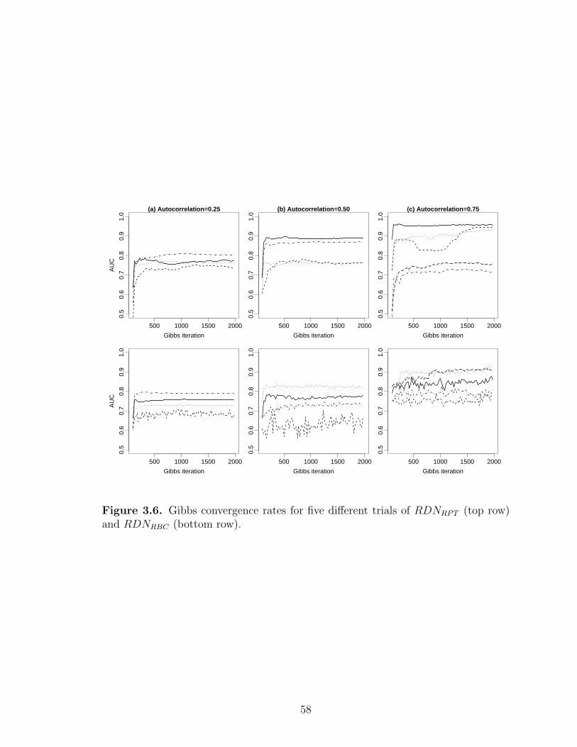
500 1000 1500 2000

0.5

0.6

0.7

0.8

0.9

1.0

(a) Autocorrelation=0.25

Gibbs iteration

AU

C

500 1000 1500 2000

0.5

0.6

0.7

0.8

0.9

1.0

(b) Autocorrelation=0.50

Gibbs iteration

500 1000 1500 2000

0.5

0.6

0.7

0.8

0.9

1.0

(c) Autocorrelation=0.75

Gibbs iteration

500 1000 1500 2000

0.5

0.6

0.7

0.8

0.9

1.0

Gibbs iteration

AU

C

500 1000 1500 2000

0.5

0.6

0.7

0.8

0.9

1.0

Gibbs iteration

500 1000 1500 2000

0.5

0.6

0.7

0.8

0.9

1.0

Gibbs iteration

Figure 3.6. Gibbs convergence rates for five different trials of RDNRPT (top row)and RDNRBC (bottom row).

58

WebKB: The data comprise 3,877 web pages from four computer science depart-

ments. The class label was page category (five values).

IMDb: The data consist of a sample of 1,382 movies released in the U.S. between

1996 and 2001. In addition to movies, the data set contain objects representing

actors, directors, and studios. The class label was opening weekend box-office

receipts (> and ≤ $2million).

Cora: The data consist of the sample of 4,330 machine-learning papers along with

associated authors, cited papers, and journals. The class label was paper topic

(seven values).

NASD: The data consist a sample of 10,000 brokers who were active in the years

1997-2001, along with approximately 12,000 associated branches, firms, and

disclosures. The class label records whether the broker will be involved in

fraud, or other serious misconduct, in the next calendar year (binary).

3.3.2.1 RDN Models

The RDNs in Figures 3.7-3.11 continue with the RDN representation introduced

in Figure 2.3b. Each item type is represented by a separate plate. An arc from x to y

indicates the presence of one or more features of x in the conditional model learned for

y. Arcs inside a plate represent dependencies among the attributes of a single object.

Arcs crossing plate boundaries represent dependencies among attributes of related

objects, with edge labels indicating the underlying relations. When the dependency

is on attributes of objects more than a single link away, the arc is labeled with a small

rectangle to indicate the intervening related-object type. For example, in Figure 3.7

paper topic is influenced by the topics of other papers written by the paper’s authors,

so the arc is labeled with two AuthoredBy relations and a small A rectangle indicating

an Author object.

59

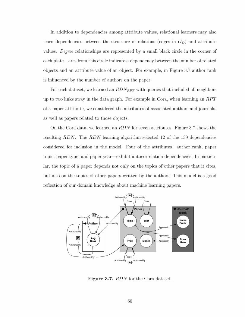
In addition to dependencies among attribute values, relational learners may also

learn dependencies between the structure of relations (edges in GD) and attribute

values. Degree relationships are represented by a small black circle in the corner of

each plate—arcs from this circle indicate a dependency between the number of related

objects and an attribute value of an object. For example, in Figure 3.7 author rank

is influenced by the number of authors on the paper.

For each dataset, we learned an RDNRPT with queries that included all neighbors

up to two links away in the data graph. For example in Cora, when learning an RPT

of a paper attribute, we considered the attributes of associated authors and journals,

as well as papers related to those objects.

On the Cora data, we learned an RDN for seven attributes. Figure 3.7 shows the

resulting RDN . The RDN learning algorithm selected 12 of the 139 dependencies

considered for inclusion in the model. Four of the attributes—author rank, paper

topic, paper type, and paper year—exhibit autocorrelation dependencies. In particu-

lar, the topic of a paper depends not only on the topics of other papers that it cites,

but also on the topics of other papers written by the authors. This model is a good

reflection of our domain knowledge about machine learning papers.

Paper

MonthType

Topic Year

Journal/Book

Name Prefix

Book Role

Author

Avg Rank

A

P

P

A

CitesCites

AuthoredBy AuthoredBy

AuthoredBy AuthoredBy

Cites

AuthoredBy AuthoredBy

AuthoredBy

AuthoredBy

AuthoredBy

AuthoredBy

AppearsIn

AppearsIn

AppearsIn

Figure 3.7. RDN for the Cora dataset.

60

Exploiting these types of autocorrelation dependencies has been shown to signif-

icantly improve classification accuracy of RMNs compared to RBNs, which cannot

model cyclic dependencies [89]. However, to exploit autocorrelation, RMNs must be

instantiated with the appropriate clique templates—to date there is no RMN algo-

rithm for learning autocorrelation dependencies. RDNs are the first PRM capable

of learning cyclic autocorrelation dependencies.

The Gene data contain attributes associated with both objects and links (i.e.,

interactions). We learned an RDN for seven attributes. Figure 3.8 shows the resulting

RDN . The RDN learning algorithm selected 19 of the 77 dependencies considered for

inclusion in the model. In these data, all the gene attributes exhibit autocorrelation—

this is strong evidence that there are regularities among the genes whose proteins

interact in the cell.

Gene

EssentialClass

Pheno-type Location

Interaction

Type

Expres-sion

Function

InteractsWith

InteractsWith

InteractsWith InteractsWith

InteractsWith InteractsWith

Figure 3.8. RDN for the Gene dataset.

On the IMDb data, we learned an RDN for ten discrete attributes. Figure 3.9

shows the resulting RDN . The RDN learning algorithm selected 29 of the 170 depen-

dencies considered for inclusion in the model. Again, we see that four of the attributes

exhibit autocorrelation. Movie receipts and genre each exhibit a number of autocor-

61

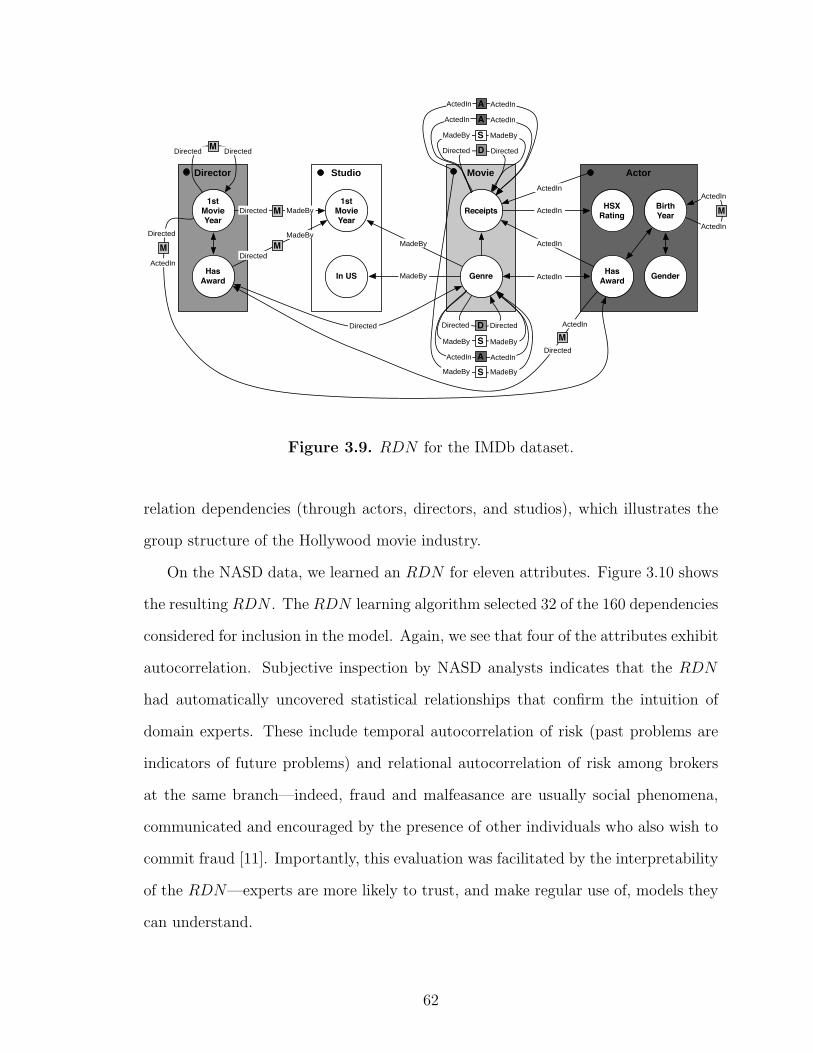
Movie

Receipts

Genre

Actor

GenderHasAward

HSX Rating

BirthYear

Director

1st MovieYear

HasAward

D

S

A

M

Studio

1st Movie Year

In US

M

M

M

M

M

DirectedDirected

Directed

ActedIn

Directed MadeBy

Directed

MadeByMadeBy

MadeBy

ActedIn

ActedIn

ActedIn

ActedIn

Directed

ActedIn

ActedIn

ActedIn

Directed

ActedIn

Directed

ActedInActedIn AS MadeByMadeBy

Directed

ActedIn

MadeByMadeBy

A ActedInActedIn

S MadeByMadeBy

D DirectedDirected

Figure 3.9. RDN for the IMDb dataset.

relation dependencies (through actors, directors, and studios), which illustrates the

group structure of the Hollywood movie industry.

On the NASD data, we learned an RDN for eleven attributes. Figure 3.10 shows

the resulting RDN . The RDN learning algorithm selected 32 of the 160 dependencies

considered for inclusion in the model. Again, we see that four of the attributes exhibit

autocorrelation. Subjective inspection by NASD analysts indicates that the RDN

had automatically uncovered statistical relationships that confirm the intuition of

domain experts. These include temporal autocorrelation of risk (past problems are

indicators of future problems) and relational autocorrelation of risk among brokers

at the same branch—indeed, fraud and malfeasance are usually social phenomena,

communicated and encouraged by the presence of other individuals who also wish to

commit fraud [11]. Importantly, this evaluation was facilitated by the interpretability

of the RDN—experts are more likely to trust, and make regular use of, models they

can understand.

62

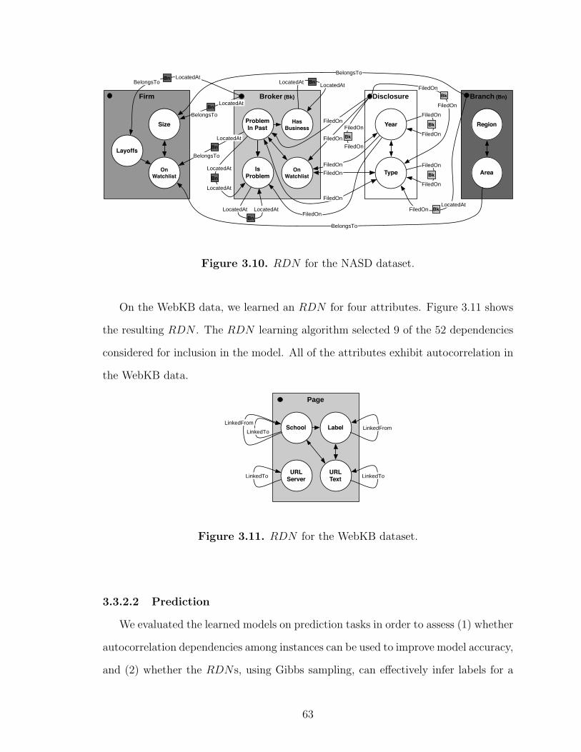
Disclosure

Year

Type

Broker (Bk)

On Watchlist

Is Problem

Problem In Past

Has Business

Firm

Size

On Watchlist

Layoffs

Branch (Bn)

Region

Area

Bk

Bk

Bk

Bn

Bn

Bn

Bn

BelongsTo

LocatedAt

BelongsTo

BelongsToLocatedAt

BnBelongsTo

LocatedAt

Bn

LocatedAt

LocatedAt

LocatedAt LocatedAt

LocatedAtLocatedAt

FiledOn

FiledOn

FiledOn

FiledOn

FiledOn

Bk

FiledOn

FiledOn

FiledOn

FiledOn

FiledOn

FiledOn

FiledOn

FiledOn

FiledOn

BkFiledOnLocatedAt

BelongsTo

Figure 3.10. RDN for the NASD dataset.

On the WebKB data, we learned an RDN for four attributes. Figure 3.11 shows

the resulting RDN . The RDN learning algorithm selected 9 of the 52 dependencies

considered for inclusion in the model. All of the attributes exhibit autocorrelation in

the WebKB data.

Page

URL Text

URL Server

School Label LinkedFrom

LinkedToLinkedTo

LinkedTo

LinkedFrom

Figure 3.11. RDN for the WebKB dataset.

3.3.2.2 Prediction

We evaluated the learned models on prediction tasks in order to assess (1) whether

autocorrelation dependencies among instances can be used to improve model accuracy,

and (2) whether the RDNs, using Gibbs sampling, can effectively infer labels for a

63

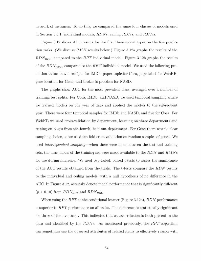
network of instances. To do this, we compared the same four classes of models used

in Section 3.3.1: individual models, RDNs, ceiling RDNs, and RMNs.

Figure 3.12 shows AUC results for the first three model types on the five predic-

tion tasks. (We discuss RMN results below.) Figure 3.12a graphs the results of the

RDNRPT , compared to the RPT individual model. Figure 3.12b graphs the results

of the RDNRBC , compared to the RBC individual model. We used the following pre-

diction tasks: movie receipts for IMDb, paper topic for Cora, page label for WebKB,

gene location for Gene, and broker is-problem for NASD.

The graphs show AUC for the most prevalent class, averaged over a number of

training/test splits. For Cora, IMDb, and NASD, we used temporal sampling where

we learned models on one year of data and applied the models to the subsequent

year. There were four temporal samples for IMDb and NASD, and five for Cora. For

WebKB we used cross-validation by department, learning on three departments and

testing on pages from the fourth, held-out department. For Gene there was no clear

sampling choice, so we used ten-fold cross validation on random samples of genes. We

used interdependent sampling—when there were links between the test and training

sets, the class labels of the training set were made available to the RDN and RMNs

for use during inference. We used two-tailed, paired t-tests to assess the significance

of the AUC results obtained from the trials. The t-tests compare the RDN results

to the individual and ceiling models, with a null hypothesis of no difference in the

AUC. In Figure 3.12, asterisks denote model performance that is significantly different

(p < 0.10) from RDNRPT and RDNRBC .

When using the RPT as the conditional learner (Figure 3.12a), RDN performance

is superior to RPT performance on all tasks. The difference is statistically significant

for three of the five tasks. This indicates that autocorrelation is both present in the

data and identified by the RDNs. As mentioned previously, the RPT algorithm

can sometimes use the observed attributes of related items to effectively reason with

64

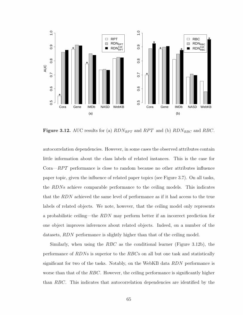
AU

C

0.5

0.6

0.7

0.8

0.9

1.0

RPTRDNRPT

RDNRPTCeil

Cora Gene IMDb NASD WebKB

(a)

*

*

*

0.5

0.6

0.7

0.8

0.9

1.0

RBCRDNRBC

RDNRBCCeil

Cora Gene IMDb NASD WebKB

(b)

*

** *

*

Figure 3.12. AUC results for (a) RDNRPT and RPT and (b) RDNRBC and RBC.

autocorrelation dependencies. However, in some cases the observed attributes contain

little information about the class labels of related instances. This is the case for

Cora—RPT performance is close to random because no other attributes influence

paper topic, given the influence of related paper topics (see Figure 3.7). On all tasks,

the RDNs achieve comparable performance to the ceiling models. This indicates

that the RDN achieved the same level of performance as if it had access to the true

labels of related objects. We note, however, that the ceiling model only represents

a probabilistic ceiling—the RDN may perform better if an incorrect prediction for

one object improves inferences about related objects. Indeed, on a number of the

datasets, RDN performance is slightly higher than that of the ceiling model.

Similarly, when using the RBC as the conditional learner (Figure 3.12b), the

performance of RDNs is superior to the RBCs on all but one task and statistically

significant for two of the tasks. Notably, on the WebKB data RDN performance is

worse than that of the RBC. However, the ceiling performance is significantly higher

than RBC. This indicates that autocorrelation dependencies are identified by the

65

RDN but the model is unable to exploit those dependencies during Gibbs sampling.

This effect is due to the amount of information available to seed the inference process.

There is sparse information in the attributes other than page label, and because the

departments are nearly disjoint, there are few labeled instances before inference. This

leaves the RDN with little information to anchor its predictions, which results in

marginal predictions closer to random. Similar behavior appeared in the synthetic

data experiments, indicating that the RDNRBC may need more information to seed

the inference process.

The RDNRBC achieves comparable performance to the ceiling models on only two

of the five tasks. This may be another indication that RDNs combined with a non-

selective conditional learner (e.g., RBCs) will experience increased variance during

the Gibbs sampling process, and thus they may need more seed information during

inference to achieve the near-ceiling performance. We should note that although the

RDNRBC does not significantly outperform the RDNRPT on any of the tasks, the

RDNCeilRBC is significantly higher than RDNCeil

RPT for Cora and IMDb. This indicates

that, when there is enough seed information, the RDNRBC may achieve significant

performance gains over the RDNRPT .

Due to time and memory constraints, we were able to learn RMNs for only two

of the real-world datasets. Recall that the RMN constructs its features from all

the attributes available to the RDN and the RMNSel constructs its features from

the attributes selected by the RDN . Table 3 reports model space information for

each dataset—the number of attributes available to the RDN , the average number

of attributes selected by the RDN , and the number of features constructed by the

RMN and the RMNSel. Due to the size of the feature space considered by the non-

selective RMNs, we were unable learn models for any of the datasets. We were able to

successfully learn RMNSel for the Cora and IMDb datasets. The average AUC of the

RMNSel was 74.4% for Cora and 60.9% for IMDb. This is far below the RDN results

66

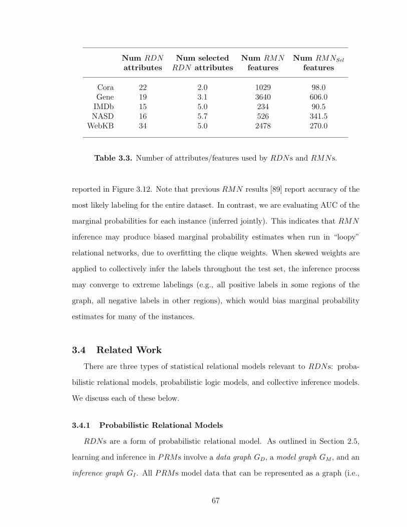
Num RDN Num selected Num RMN Num RMNSel

attributes RDN attributes features features

Cora 22 2.0 1029 98.0Gene 19 3.1 3640 606.0

IMDb 15 5.0 234 90.5NASD 16 5.7 526 341.5

WebKB 34 5.0 2478 270.0

Table 3.3. Number of attributes/features used by RDNs and RMNs.

reported in Figure 3.12. Note that previous RMN results [89] report accuracy of the

most likely labeling for the entire dataset. In contrast, we are evaluating AUC of the

marginal probabilities for each instance (inferred jointly). This indicates that RMN

inference may produce biased marginal probability estimates when run in “loopy”

relational networks, due to overfitting the clique weights. When skewed weights are

applied to collectively infer the labels throughout the test set, the inference process

may converge to extreme labelings (e.g., all positive labels in some regions of the

graph, all negative labels in other regions), which would bias marginal probability

estimates for many of the instances.

3.4 Related Work

There are three types of statistical relational models relevant to RDNs: proba-

bilistic relational models, probabilistic logic models, and collective inference models.

We discuss each of these below.

3.4.1 Probabilistic Relational Models

RDNs are a form of probabilistic relational model. As outlined in Section 2.5,

learning and inference in PRMs involve a data graph GD, a model graph GM , and an

inference graph GI . All PRMs model data that can be represented as a graph (i.e.,

67

GD) and although PRMs use different approximation techniques for inference in GI ,

they all use a similar process for rolling out an inference graph GI . Consequently,

PRMs differ primarily with respect to the representation of the model graph GM ,

how that model is learned, and the choice of inference algorithm.

Relational Bayesian Networks

RBNs [29] use a directed model graph GM = (VM , EM) and a set of conditional

probability distributions P to represent a joint distribution over X. Each node v ∈ VM

corresponds to an X tk ∈ X. The set P contains a conditional probability distribution

for each variable given its parents, p(xtk|paxt

k). Given (GM , P ), the joint probability

for a set of values x is computed as a product over the item types T , the attributes

of that type X t, and the items of that type v, e:

p(x) =∏t∈T

∏Xt

i∈Xt

∏v:T (v)=t

p(xtvi|paxt

vi)

∏e:T (e)=t

p(xtei|paxt

ei)

The RBN learning algorithm for the most part uses standard Bayesian network

techniques for parameter estimation and structure learning. One notable exception is

that the learning algorithm must check for “legal” structures that are guaranteed to

be acyclic when rolled out for inference on arbitrary data graphs. In addition, instead

of exhaustive search of the space of relational dependencies, the structure learning

algorithm uses greedy iterative-deepening, expanding the search in directions where

the dependencies improve the likelihood.

The strengths of RBNs include understandable knowledge representations and

efficient learning techniques. For relational tasks, with a huge space of possible de-

pendencies, selective models are easier to interpret and understand than non-selective

models. Closed-form parameter estimation techniques allow for efficient structure

learning (i.e., feature selection). In addition, because reasoning with relational mod-

68

els requires more space and computational resources, efficient learning techniques

make relational modeling both practical and feasible.

The directed acyclic graph structure is the underlying reason for the efficiency

of RBN learning. As discussed previously, the acyclicity requirement precludes the

learning of arbitrary autocorrelation dependencies and limits the applicability of these

models in relational domains. RDNs enjoy the strengths of RBNs (namely, under-

standable knowledge representation and efficient learning) without being constrained

by an acyclicity requirement.

Relational Markov Networks

RMNs [89] use a undirected model graph UM = (VM , EM) and a set of potential

functions Φ to represent a joint distribution over X. Again each node v ∈ VM corre-

sponds to an X tk ∈ X. RMNs use relational clique templates CT to specify the ways

in which cliques are defined in UM . Clique templates are defined over a set of item

types, a boolean constraint on how the types must relate to each other in the data

graph, and a set of attributes to consider on the matching items. Let C(CT ) be the

set of cliques in the graph UM that match a specific clique template CT . As with

Markov networks, each clique c ∈ C(CT ) is associated with a set of variables Xc and

a clique potential φc(xc). Given (UM , Φ), the joint probability for a set of values x is

computed as a product over the clique templates CT and the matches to the clique

template c:

p(x) =1

Z

∏Ci∈CT

∏cj∈Ci

φcj(xcj

)

The RMN learning algorithm uses maximum-a-posteriori parameter estimation

with Gaussian priors, modifying Markov network learning techniques. The algorithm

assumes that the clique templates are pre-specified and thus does not search for the

best structure. Because the user supplies a set of relational dependencies to consider

69

(i.e., clique templates), it simply optimizes the potential functions for the specified

templates.

RMNs are not hampered by an acyclicity constraint, so they can represent arbi-

trary forms of autocorrelation. This is particularly important for reasoning in rela-

tional datasets where autocorrelation dependencies are nearly ubiquitous and often

cannot be structured in an acyclic manner. However, the tradeoff for this increased

representational capability is a decrease in learning efficiency. Instead of closed-form

parameter estimation, RMNs are trained with conjugate gradient methods, where

each iteration requires a round of inference. In large cyclic relational inference graphs,

the cost of inference is prohibitively expensive—in particular, without approximations

to increase efficiency, feature selection is intractable.

Similar to the comparison with RBNs, RDNs enjoy the strengths of RMNs but

not their weaknesses. More specifically, RDNs are able to represent arbitrary forms of

autocorrelation without being limited by efficiency concerns during learning. In fact,

the pseudolikelihood estimation technique used by RDNs has been used recently to

make feature selection tractable for conditional random fields [58] and Markov logic

networks [48].

3.4.2 Probabilistic Logic Models

Within the class of PLMs, Markov logic networks (MLNs) [83] are most similar

in nature to RDNs. In MLNs, each node is a grounding of a predicate in a first-order

knowledge base, and features correspond to first-order formulae and their truth values.

An MLN , unrolled over a set of objects in the domain, specifies an undirected Markov

network. In this sense, they share the same strengths and weaknesses as RMNs—

they are capable of representing cyclic autocorrelation relationships but suffer from

decreased efficiency if full joint estimation is used during learning.

70

Recent work on structure learning for MLNs [48] has investigated the use of pseu-

dolikelihood to increase learning efficiency. The MLN structure learning algorithm

restricts the search space by limiting the number of distinct variables in a clause, and

then uses beam search, with a weighted pseudolikelihood scoring function, to find the

best clauses to add to the network.

Although both RDNs and MLNs use pseudolikelihood techniques to learn model

structures efficiently, they each employ a different representational formalism. In

particular, MLNs use weighted logic formulae while RDNs use aggregate features

in CPDs. Our future work will investigate the performance tradeoffs between RDN

and MLN representations when pseudolikelihood estimation is used for learning.

3.4.3 Ad hoc Collective Models

An alternative approach to collective inference combines local individual classifica-

tion models (e.g., RBCs) with a joint inference procedure (e.g., relaxation labeling).

Examples of this technique include iterative classification [67], link-based classifica-

tion [54], and probabilistic relational neighbor models [55, 56]. These approaches

to collective inference were developed in an ad hoc procedural fashion, motivated

by the observation that they appear to work well in practice. RDNs formalize this

approach in a principled framework—learning models locally (maximizing pseudolike-

lihood) and combining them with a global inference procedure (Gibbs sampling) to

recover a full joint distribution. In this work, we have demonstrated that autocorre-

lation is the reason behind improved performance in collective inference (see Jensen

et al. [42] for more detail) and explored the situations under which we can expect this

type of approximation to perform well.

71

3.5 Conclusion

In this chapter, we presented relational dependency networks, a new form of prob-

abilistic relational model. We showed the RDN learning algorithm to be a relatively

simple method for learning the structure and parameters of a probabilistic graphical

model. In addition, RDNs allow us to exploit existing techniques for learning condi-

tional probability distributions of relational datasets. Here we have chosen to exploit

our prior work on RPT s, which construct parsimonious models of relational data, and

RBCs, which are simple and surprisingly effective non-selective models. We expect

the general properties of RDNs to be retained if other approaches to learning condi-

tional probability distributions are used, given that those approaches learn accurate

local models.

The primary advantage of RDNs is the ability to efficiently learn autocorrela-

tion dependencies. Autocorrelation is a nearly ubiquitous phenomenon in relational

datasets and the resulting dependencies are often cyclic in nature. If a dataset exhibits

autocorrelation, an RDN can learn the associated dependencies and then exploit

those dependencies to improve overall inferences by collectively inferring values for

the entire set of instances simultaneously. The real and synthetic data experiments in

this chapter show that collective inference with RDNs can offer significant improve-

ment over individual approaches when autocorrelation is present in the data. Except

in cases when there are few test set labels, the performance of RDNs approaches the

performance that would be possible if all the class labels of related instances were

known. Furthermore, our experiments show that inference with RDNs is comparable,

or superior, to RMN inference over a range of conditions, which indicates that pseu-

dolikelihood estimation can be used effectively to learn an accurate approximation of

the full joint distribution.

We also presented learned RDNs for a number of real-world relational domains,

demonstrating another strength of RDNs—their understandable and intuitive knowl-

72

edge representation. Comprehensible models are a cornerstone of the knowledge dis-

covery process, which seeks to identify novel and interesting patterns in large datasets.

Domain experts are more willing to trust, and make regular use of, understandable

models—particularly when the induced models are used to support additional rea-

soning. Understandable models also aid analysts’ assessment of the utility of the

additional relational information, potentially reducing the cost of information gath-

ering and storage and the need for data transfer among organizations—increasing the

practicality and feasibility of relational modeling.

73

CHAPTER 4

LATENT GROUP MODELS

Our recent work investigating how collective inference improves classification has

illustrated the effect of model representation on performance in relational domains [42].

More specifically, we showed that modeling the direct dependencies among class labels

of related instances is a low-variance means of reducing model bias when autocorre-

lation is present. An alternative approach is to model the dependencies among class

labels indirectly through their association with the observed attributes of related in-

stances, but this approach experiences a dramatic increase in variance as the number

of observed attributes increases.

In this work, we have shown that direct modeling with RDNs can lead to sig-

nificant improvements in performance over individual models in domains with even

modest amounts of autocorrelation. However, this approach fails to capture a frequent

characteristic of autocorrelated data—the presence of underlying groups, conditions,

or events that are correlated with the attributes on a set of entities. Models that rep-

resent the underlying group structure and the association between unobserved group

properties and observed attribute values and links may be able to express the joint

distribution more accurately and compactly than approaches that only model direct

dependencies among class labels.

Recall the fragment of the NASD database, where brokers exhibit autocorrelation

with respect to their fraud status. For reference, we include the graphic again in

Figure 4.1(a). The autocorrelation in this example can be represented through the

underlying group structure of the data. In Figure 4.1(b), groups of brokers that work

74

-

-

-

-

- - -

- - -

+

++

- -

+

-

-

+

-

-

- -

-

-

+

+

- +

+ +

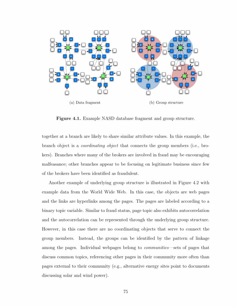
(a) Data fragment

-

-

-

-

- - -

- - -

+

++

- -

+

-

-

+

-

-

- -

-

-

+

+

- +

+ +

(b) Group structure

Figure 4.1. Example NASD database fragment and group structure.

together at a branch are likely to share similar attribute values. In this example, the

branch object is a coordinating object that connects the group members (i.e., bro-

kers). Branches where many of the brokers are involved in fraud may be encouraging

malfeasance; other branches appear to be focusing on legitimate business since few

of the brokers have been identified as fraudulent.

Another example of underlying group structure is illustrated in Figure 4.2 with

example data from the World Wide Web. In this case, the objects are web pages

and the links are hyperlinks among the pages. The pages are labeled according to a

binary topic variable. Similar to fraud status, page topic also exhibits autocorrelation

and the autocorrelation can be represented through the underlying group structure.

However, in this case there are no coordinating objects that serve to connect the

group members. Instead, the groups can be identified by the pattern of linkage

among the pages. Individual webpages belong to communities—sets of pages that

discuss common topics, referencing other pages in their community more often than

pages external to their community (e.g., alternative energy sites point to documents

discussing solar and wind power).

75

-

+

+

+

+

+

+

+

+

+

+

+

++

+

+

+

+

+

+

+

-

-

-

-

-

-

-

-

-

-

--

--

-

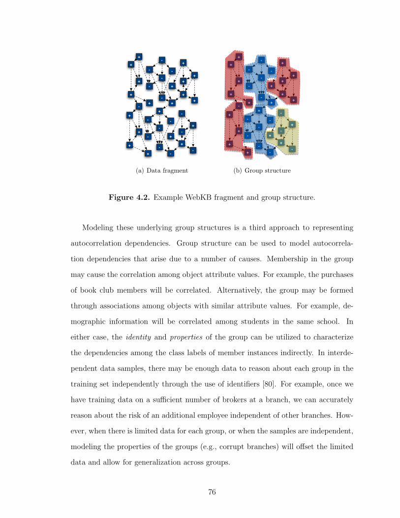
(a) Data fragment

-

+

+

+

+

+

+

+

+

+

+

+

++

+

+

+

+

+

+

+

-

-

-

-

-

-

-

-

-

-

--

--

-

(b) Group structure

Figure 4.2. Example WebKB fragment and group structure.

Modeling these underlying group structures is a third approach to representing

autocorrelation dependencies. Group structure can be used to model autocorrela-

tion dependencies that arise due to a number of causes. Membership in the group

may cause the correlation among object attribute values. For example, the purchases

of book club members will be correlated. Alternatively, the group may be formed

through associations among objects with similar attribute values. For example, de-

mographic information will be correlated among students in the same school. In

either case, the identity and properties of the group can be utilized to characterize

the dependencies among the class labels of member instances indirectly. In interde-

pendent data samples, there may be enough data to reason about each group in the

training set independently through the use of identifiers [80]. For example, once we

have training data on a sufficient number of brokers at a branch, we can accurately

reason about the risk of an additional employee independent of other branches. How-

ever, when there is limited data for each group, or when the samples are independent,

modeling the properties of the groups (e.g., corrupt branches) will offset the limited

data and allow for generalization across groups.

76

In this chapter, we describe latent group models (LGMs). LGMs represent a joint

probability distribution over both the attributes and links of a relational dataset, in-

corporating link existence uncertainty and hierarchical latent variables. LGMs posit

groups of objects in the data—membership in these groups influences the observed

attributes of the objects, as well as the existence of links among the objects. LGMs

address a number of weaknesses of current collective inference models. First, LGMs

extend recent PRM representations to model link structure and autocorrelation de-

pendencies indirectly through the hidden group structures. These group structures

enable the incorporation of link information into PRMs in a more tractable way than

PRMs with link uncertainty [30] because group membership decouples attribute and

link dependencies. Second, the group structures can capture dependencies among

neighboring but unlinked instances (e.g., transitive relationships), allowing informa-

tion to propagate in a more elaborate manner during inference than with models that

restrict their consideration to dependencies among closely linked instances. Group

models are a natural way to extend PRM representations to improve model per-

formance without fully representing the O(N2) dependencies between all pairs of

instances. Third, LGMs generalize about the properties of groups. This is in con-

trast to recent work modeling specific groups and objects in the training set to im-

prove classification performance in interdependent samples [81, 80]. Consequently,

learned LGMs can be applied to prediction tasks in both interdependent and inde-

pendent samples. Finally, LGMs recover the underlying group structure, which can

be examined to improve domain understanding and inform development of additional

modeling techniques.

We start by discussing the latent group model representation and then describe

a specific implementation that we utilize throughout the thesis. We evaluate LGM

inference on synthetic datasets, showing that LGMs outperform RDNs and RMNs

in a range of conditions, particularly when there are moderate-sized clusters with

77

low linkage. Next, we present empirical evaluation of LGMs on three real-world

prediction tasks to demonstrate the capabilities of the model, showing that LGMs

can outperform models that ignore latent groups, particularly when there is little

known information with which to seed the inference process. Finally, we discuss

related work and conclude.

4.1 Latent Group Models

Latent group models specify a generative probabilistic model for the attributes

and link structure of a relational dataset. The model posits groups of objects in the

data of various types. Membership in these groups influences the observed attributes

of objects, as well as the existence of relations (links) among objects.

4.1.1 LGM Representation

The LGM extends the PRM representation outlined in Section 2.5 to model a

joint distribution over both the attributes and links of a relational dataset. To model

link uncertainty, we include an augmented edge set E ′ that contains an edge for every

pair of objects in the data (∀vi, vj ∈ VD eij ∈E ′) with a binary link variable XL to

indicate whether a relation exists between the incident objects.1 In addition to the

objects and links in the data, we also model a set of groups G. As with objects and

links, each group is associated with a type, T (gi) = tgiand a set of attributes based

on that type Xtgigi . Each object vi ∈ VD belongs to a set of groups gvi

= (gvi1, ..., gvik).

Group membership and properties (i.e., attributes) can influence the values of object

attributes, link attributes, and link existence. An LGM represents a joint distribution

over the values of the attributes in the data, x = xtvivi : vi ∈ VD s.t. T (vi) = tvi

∪

xtejej : ej ∈ ED s.t. T (ej) = tej

∪ xekL : ek ∈ E ′ ∪ xtglgl : gl ∈ G s.t. T (gl) = tgl

.

1We assume binary links and at most one link between any pair of objects. However, it isrelatively straightforward to extend the model to accommodate deviations from these assumptions.

78

There are two steps to incorporating groups and their properties into PRMs.

First, we need to detect the underlying group structure. When the groups are iden-

tified by a coordinating object (e.g., branch), detection is a relatively easy task—we

can identify groups through high degree nodes and their immediate neighbors. When

groups consist of communities, group detection is more difficult. However, if intra-

community links are more frequent than inter-community links, the existing relations

can be used as evidence of the underlying community structure, and group member-

ship can be inferred from the patterns of relations.

Next, we need to infer the latent group properties and model their influence on the

attributes and relations of group members. When the groups are observable, we can

model the latent attributes with a relatively simple application of the expectation-

maximization (EM) algorithm [15]. A similar approach is used in information retrieval

where latent-unigram models represent each document as a group of word occurrences2

that are conditionally independent given the topic of the document [6].

When groups are unobserved, group membership and properties must be jointly

inferred from the observed relations and attributes. To continue the document re-

trieval metaphor, it is as if we have word occurrence information (attribute values)

and noisy indicators of word co-occurrence within documents (link information) but

we do not know the document boundaries or the topic distributions. In these sit-

uations, an iterative procedure may be necessary to recover group membership and

infer latent group properties.

For our initial investigation of LGMs, we make several simplifying assumptions

about the data. We assume a unipartite relational data graph (i.e., single object and

link type) and that there are no link attributes other than XL. We also assume there

is one group type with one attribute and that each object belongs to a single group.

2However, the “vocabulary” is much smaller in relational domains—we generally have fewer thanten class values, whereas documents have thousands of unique words.

79

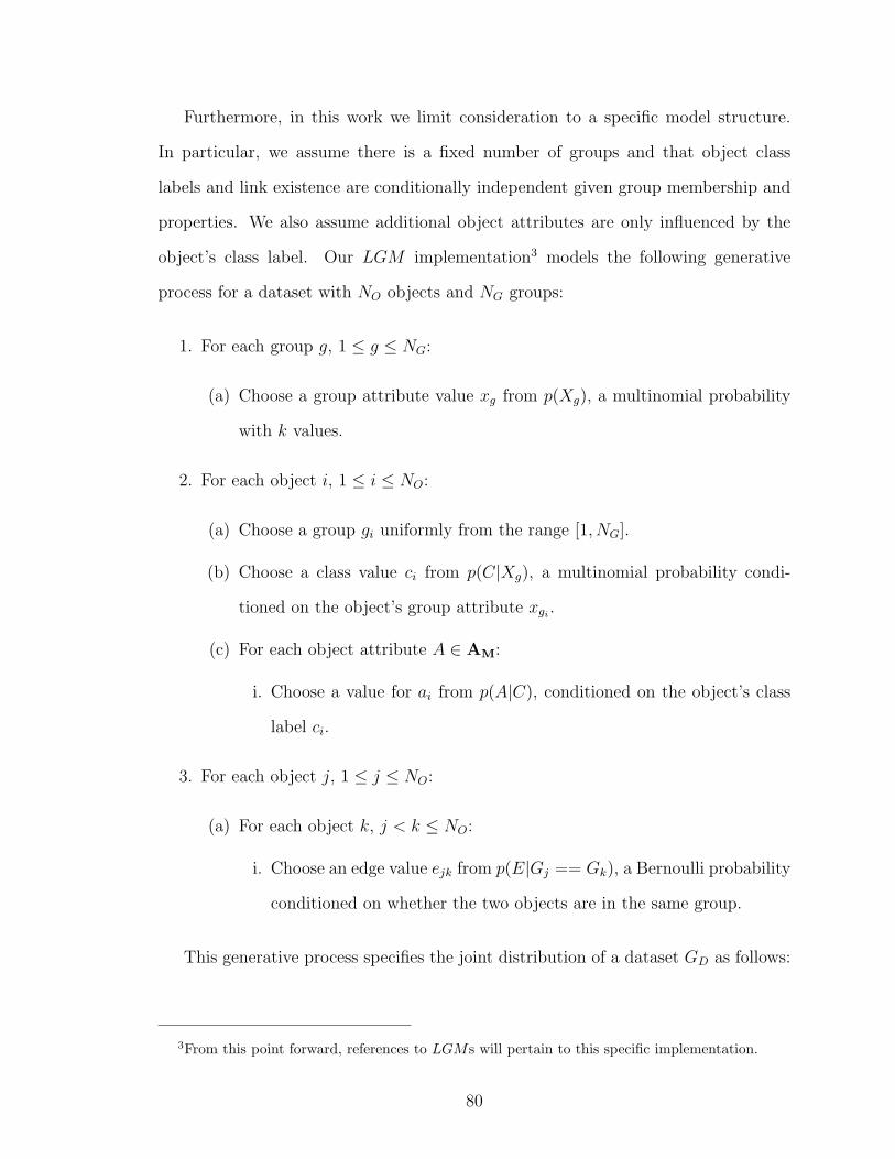
Furthermore, in this work we limit consideration to a specific model structure.

In particular, we assume there is a fixed number of groups and that object class

labels and link existence are conditionally independent given group membership and

properties. We also assume additional object attributes are only influenced by the

object’s class label. Our LGM implementation3 models the following generative

process for a dataset with NO objects and NG groups:

1. For each group g, 1 ≤ g ≤ NG:

(a) Choose a group attribute value xg from p(Xg), a multinomial probability

with k values.

2. For each object i, 1 ≤ i ≤ NO:

(a) Choose a group gi uniformly from the range [1, NG].

(b) Choose a class value ci from p(C|Xg), a multinomial probability condi-

tioned on the object’s group attribute xgi.

(c) For each object attribute A ∈ AM:

i. Choose a value for ai from p(A|C), conditioned on the object’s class

label ci.

3. For each object j, 1 ≤ j ≤ NO:

(a) For each object k, j < k ≤ NO:

i. Choose an edge value ejk from p(E|Gj == Gk), a Bernoulli probability

conditioned on whether the two objects are in the same group.

This generative process specifies the joint distribution of a dataset GD as follows:

3From this point forward, references to LGMs will pertain to this specific implementation.

80

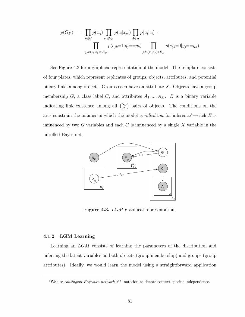
p(GD) =∏g∈G

p(xg)∏

vi∈VD

p(ci|xgi)

∏A∈A

p(ai|ci) ·∏j,k:(vi,vj)∈ED

p(ejk=1|gj==gk)∏

j,k:(vi,vj)/∈ED

p(ejk=0|gj==gk)

See Figure 4.3 for a graphical representation of the model. The template consists

of four plates, which represent replicates of groups, objects, attributes, and potential

binary links among objects. Groups each have an attribute X. Objects have a group

membership G, a class label C, and attributes A1, ..., AM . E is a binary variable

indicating link existence among all(

NO

2

)pairs of objects. The conditions on the

arcs constrain the manner in which the model is rolled out for inference4—each E is

influenced by two G variables and each C is influenced by a single X variable in the

unrolled Bayes net.

NO

Ejk

Gi

Ci

Ai

M

Xg

NG

NG

j=i

g=Gi

k=i'

( )NO2

Figure 4.3. LGM graphical representation.

4.1.2 LGM Learning

Learning an LGM consists of learning the parameters of the distribution and

inferring the latent variables on both objects (group membership) and groups (group

attributes). Ideally, we would learn the model using a straightforward application

4We use contingent Bayesian network [62] notation to denote context-specific independence.

81

of the EM algorithm—iterating between inferring the latent variables (E-step) and

estimating the parameters (M-step). Unfortunately, there are difficulties with this

approach.

When group membership is unknown, each of the C variables depends on all the

X variables and each of the E variables depends on all the G variables—there is no

longer context-specific independence to exploit and each E-step will require inference

over a large, complex, rolled-out Bayes net where objects’ group memberships are

all interdependent given the link observations. Although approximate inference tech-

niques (e.g., loopy belief propagation) may allow accurate inference in each E-step,

given the number of latent variables and their dependency on sparse link informa-

tion (L(

NO

2

)), we conjecture that EM will not converge to a reasonable solution

due to many local (suboptimal) maxima in the likelihood function. Also when using

EM to learn the entire model, there are NO latent group membership variables with

NG possible values and NG latent group attribute values with k possible values. If

the average group size is small (NG = O(NO)), we conjecture that EM will be very

sensitive to the start state.

We note however, that if group membership is known, then exact inference is not

only feasible but is also much more efficient. This is because the objects and ob-

served links are conditionally independent given the underlying group structure. For

this reason we propose a sequential learning procedure that decouples group identi-

fication from the remainder of the estimation process. Our algorithm is motivated

by the observation that collective models improve performance by propagating in-

formation only on existing links. This indicates that autocorrelated groups should

have more intra-group links than inter-group links and as such, graph clustering tech-

niques should be able to identify groups from the link structure alone. Accordingly,

we utilize the following approximate learning algorithm:

1. Hypothesize group membership for objects based on the observed link structure.

82

2. Use EM to infer group attributes and estimate the remaining parameters of the

model.

A hard clustering approach in the first step, which assigns each object to a single

group, greatly simplifies the estimation problem in the second step—we only need to

infer the latent group attribute values and estimate the parameters of p(X), p(C|X),

and p(Ai|C) for 1 ≤ i ≤ m. To this end, we employ a recursive spectral decomposition

algorithm with a norm-cut objective function [86] to cluster the objects into groups

with high intra-group and low inter-group linkage.

Spectral clustering techniques partition data into disjoint clusters using the eigen-

structure of a similarity matrix. We use the divisive, hierarchical clustering algorithm

of [86] on the relational graph formed by the observed links in the data. The algorithm

recursively partitions the graph as follows: Let EN×N = [E(i, j)] be the adjacency ma-

trix and let D be an N ×N diagonal matrix with di =∑

j∈V E(i, j). Solve the eigen-

system (D−E)x = λDx for the eigenvector x1 associated with the 2nd smallest eigen-

value λ1. Consider m uniform values between the minimum and maximum value in x1.

For each value m: bipartition the nodes into (A, B) such that ∀va∈A x1a <m, and cal-

culate the NCut value for the partition, NCut(A, B)=P

i∈A,j∈B E(i,j)Pi∈A di

+P

i∈A,j∈B E(i,j)Pj∈B dj

.

Partition the graph into the (A, B) with minimum NCut. If stability(A, B)≤ c, re-

cursively repartition A and B.5

Once we have identified the groups with spectral clustering, we use EM to infer

values for X and estimate the parameters of P (X) and P (C|X). We iterate the

following steps until the probability distributions have converged to within a tolerance

of 0.001:

E-step t + 1: Infer values for X t+1 with P t+1(xg|cg) =∏

ci:g=Gi

P t(ci|xg)P t(xg)

P (ci)

5We use the stability threshold proposed in [86] where the stability value is the ratio ofthe minimum and maximum bin sizes, after the values of x1 are binned by value into mbins. Unless otherwise noted, we use m = dlog2(N) + 1e and c = 0.06.

83

M-step t + 1: Calculate maximum likelihood estimates for P t+1(X) and P t+1(C|X)

using the inferred values of X t+1

In addition, we estimate the parameters of P (Ai|C) for 1 ≤ i ≤ m. Because

the object attributes are conditionally independent of the group attributes given the

objects’ class labels, we do not need to use EM to estimate these CPDs.

As we show in Section 4.2, our sequential learning approach appears to work

well in practice. However, refinements to iterate the clustering and EM steps, or to

incorporate soft clusterings, may improve results even further.

4.1.3 LGM Inference

When applying an LGM for prediction, the class labels C, group membership

G, and group attributes X are all unobserved and must be inferred. Our inference

algorithm is similar to the sequential learning procedure:

1. Hypothesize group membership for objects based on the observed link structure.

2. Use belief propagation to infer group attributes and object class labels jointly.

We begin by using spectral clustering to identify the groups using the observed

links. This simplifies inference by partitioning the objects into disjoint sets and fixing

their group memberships. Then inference can be decomposed into disjoint subtasks,

one for each group. Within each group, the class labels are conditionally independent

given the group attribute values so exact inference is possible. We use standard belief

propagation [78] to jointly infer group attributes and class labels.

4.2 Experimental Evaluation

The experiments in this section demonstrate the utility of latent group models in

relational domains. First, we use synthetic datasets to explore the conditions under

which LGMs improve performance over comparable collective models. We vary the

84

clustering and linkage of the data, showing that LGMs improve performance when

intra-group linkage is sparse or when there is little information to seed inference.

Next, we evaluate LGMs on three real-world prediction tasks, showing that LGMs

can leverage autocorrelation to improve model accuracy. Again, we show that LGMs

achieve significant performance gains when there is less information available to seed

the inference process.

LGMs can be used for prediction tasks in both interdependent and independent

samples. In interdependent samples there may be enough information about the class

distribution associated with the groups in the training set for group membership to

improve inference without inferring group attributes. There are a number of relational

learning approaches [87, 81, 80] that use group identities in the training set to improve

inference in these situations. In independent samples, it is necessary to generalize

about group properties to improve performance. LGMs are the first prediction model

to generalize about group properties, thus we expect LGMs will be most useful for

prediction tasks in independent samples. For this reason, we focus our evaluation

primarily in this context. Independent samples reflect a number of relevant relational

domains. For example, independent samples can be used to develop models of web

pages on localized sites for application on the broader World Wide Web. Alternatively,

independent samples can be used to develop fraud detection models on data from a

single city for application on branches and brokers in the remainder of the country.

Finally, independent samples can be used to develop gene prediction models on a

genome from a single organism for application on other related organisms.

4.2.1 Synthetic Data Experiments

To explore the effects of graph structure on LGM inference, we generated ho-

mogeneous data graphs with an autocorrelated class label and linkage due to the

underlying group structure. Each object has four boolean attributes: X1, X2, X3

85

and X4. We varied linkage and group size and learned models to predict X1. See

appendix A.1.2 for a detailed description of the data generation process.

More specifically, we generated data with small and large groups sizes, and high

and low levels of linkage. The first set of data have small group size and low linkage,

thus we expect it will be difficult to exploit the autocorrelation in the data due to

low connectivity. The second set of data have small group size but high linkage,

thus we expect it will be easier to exploit neighbor information but that it may be

difficult to identify the underlying groups. The third set of data have large group

size and low linkage. We expect the LGMs will be more accurate on data with large

group sizes because they can incorporate information from a wider neighborhood

than RDNs and RMNs, which use only local neighbor information. The fourth set

of data have large group size and high linkage—we expect that models will be able to

exploit autocorrelation dependencies most effectively in these data, due to the high

connectivity and clustering.

Figure 4.4 graphs a sample synthetic dataset with small group size and high

linkage. The final datasets are homogeneous—there is only one object type and one

link type, and each object has four attributes. After the groups are used to generate

the data, we delete them from the data—the groups are not available for model

learning or inference.

We compare the performance of LGMs to five different models. The first two

models are RDNs and RMNs. These models use the intrinsic attributes of objects,

the observed attributes of directly related objects, and the class labels of directly

related objects to predict X1.

The third model (RDNGrp) is a modification of the RDN , which incorporates the

groups discovered in the LGM clustering. More specifically, we augment the dataset

so that each pair of group members are directly linked before we learn an RDNGrp.

This model demonstrates the utility of propagating information among distant group

86

Figure 4.4. Sample synthetic dataset.

members in an RDN . In addition to the attributes used by the RDN and the RMN ,

the RDNGrp also uses the class labels and observed attributes of group members to

model X1.

The fourth model (LGMRand) is a modification of the LGM , which uses random

groups rather than the groups discovered by the spectral clustering component. We

include LGMRand to illustrate the utility of the identified groups.

The fifth model (wvRN) is a weighted-vote relational neighbor classifier [55, 56].

wvRN is an iterative collective model that estimates an object’s class probabilities

using the weighted mean of the class-membership probabilities of the object’s neigh-

bors. We include wvRN as a baseline autocorrelation model that uses only the class

labels in the data graph.

Figure 4.5 shows AUC results for each of the models on the four different types

of data. During inference, we varied the number of known class labels available to

seed the inference process by randomly labeling a portion (0.0, 0.3, 0.6) of the test

set instances. We expect performance to be similar when other information serves

to seed the inference process—either when some labels can be inferred from intrinsic

attributes, or when weak predictions about many related instances serve to constrain

the system. At each level of labeling, we generated five test sets. For each test set, we

87

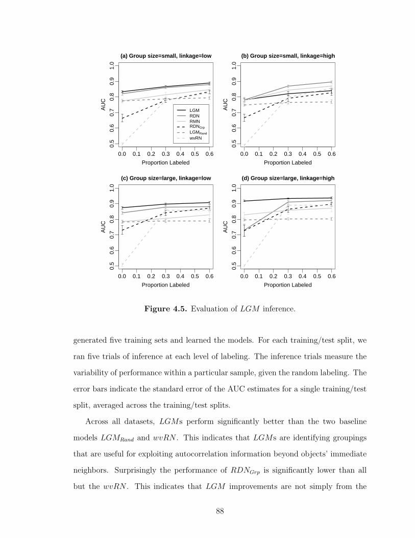
0.0 0.1 0.2 0.3 0.4 0.5 0.6

0.5

0.6

0.7

0.8

0.9

1.0

(a) Group size=small, linkage=low

Proportion Labeled

AU

CLGMRDNRMNRDNGrp

LGMRand

wvRN

0.0 0.1 0.2 0.3 0.4 0.5 0.6

0.5

0.6

0.7

0.8

0.9

1.0

(b) Group size=small, linkage=high

Proportion Labeled

AU

C

0.0 0.1 0.2 0.3 0.4 0.5 0.6

0.5

0.6

0.7

0.8

0.9

1.0

(c) Group size=large, linkage=low

Proportion Labeled

AU

C

0.0 0.1 0.2 0.3 0.4 0.5 0.6

0.5

0.6

0.7

0.8

0.9

1.0

(d) Group size=large, linkage=high

Proportion Labeled

AU

C

Figure 4.5. Evaluation of LGM inference.

generated five training sets and learned the models. For each training/test split, we

ran five trials of inference at each level of labeling. The inference trials measure the

variability of performance within a particular sample, given the random labeling. The

error bars indicate the standard error of the AUC estimates for a single training/test

split, averaged across the training/test splits.

Across all datasets, LGMs perform significantly better than the two baseline

models LGMRand and wvRN . This indicates that LGMs are identifying groupings

that are useful for exploiting autocorrelation information beyond objects’ immediate

neighbors. Surprisingly the performance of RDNGrp is significantly lower than all

but the wvRN . This indicates that LGM improvements are not simply from the

88

linking up of distant neighboring objects in the data. The model representation

(e.g., conditional independence of class given group) must also contribute to the

performance gains.

When group size is small and linkage is low, LGMs perform only slightly better

than RDNs, which indicates that the groups are too small for the LGM to signifi-

cantly capitalize on group information.

When group size is small and linkage is high, LGMs are outperformed by both

RDNs and RMNs when the test set is at least partially labeled. The LGMs’ poor

performance on these data is due to the learning algorithm’s inability to identify the

latent group structure. When the density of linkage between groups is relatively high

compared to the average group size, it is difficult for the spectral clustering algorithm

to correctly identify the fine grained underlying group structure.

When group size is large, LGMs outperform the other models regardless of linkage.

In these data, the larger groups allow LGMs to propagate information farther in the

graph than RDNs and RMNs, which use only local neighbor information. The most

significant improvement is when linkage is high and there are no labeled instances in

the test set. This indicates that LGMs can aggregate sparse attribute information

across wide neighborhoods to offset the lack of class label information.

4.2.2 Empirical Data Experiments

We present results for two LGM variations. The first variation, LGMk, sets the

number of group attribute values to the number of class label values, k = |C| (e.g., for

binary tasks, k = 2); the second variation, LGM2k, sets k = 2|C|. We compare the

LGM to four alternative models. The first two are individual inference models: the

RPT and the RBC. The third model is an RDNRPT . The fourth model (RDNCeilRPT )

is a probabilistic ceiling for the RDNRPT , where we allow the true labels of related

instances to be used during inference. This model shows the level of performance

89

possible if the RDNRPT could infer the true labels of related instances with perfect

accuracy.

The first set of experiments considers the restricted task of predicting class labels

using only the class labels of related instances and/or the group membership. This

limits confounding effects due to feature construction and model selection. The mod-

els do not have equivalent feature spaces, nor do they all perform feature selection,

but the differences are minimized when the models are restricted to consider a small

number of attributes (i.e., class label and/or group membership). A second set of

experiments includes object attributes in each of the models to evaluate the impact

of intrinsic attribute information on performance.

For the RPT s and RBCs, we clustered the training and test sets together and

used cluster ID as the sole attribute in the model. The performance of these models

illustrates the baseline utility of clustering without typing the groups and serves as

a comparison to previous work [81], which clusters the data to generate additional

features for prediction. For the LGM , RDNRPT and RDNCeilRPT , we used the class

label of related instances as the sole attribute available for modeling. When possible

we used exact inference, but for RDNs, which require approximate inference, we used

Gibbs with chains of length 500 and burn-in of 100. (At this length, accuracy and

AUC had seemingly converged.) During inference we again varied the number of

known class labels available to seed the inference process.

We compared the six models on three relational datasets (see appendix A.1.3 for

a more detailed description of the data):

WebKB: We considered the unipartite co-citation web graph. The class label was

page category (five values). As in previous work on this dataset, we do not try

to predict the category Other ; we remove them from the data after creating the

co-citation graph.

90

IMDb: We considered a unipartite graph of 1,382 movies released in the U.S. between

1996 and 2001, where links indicate movies that are made by a common studio.

The class label was opening weekend box-office returns (binary).

Cora: We considered the unipartite co-citation graph of 4,330 machine-learning pa-

pers. The class label was paper topic (seven values).

Figure 4.6 shows AUC results for each of the models on the three prediction

tasks when the models do not use additional attributes. The graph shows AUC for

the most prevalent class, averaged over the training/test splits.6 For WebKB, we

used cross-validation by department, learning on three departments and testing on

the fourth. For IMDb, we used snowball sampling [32] to bipartition the data into

five disjoint training/test samples. For Cora, we used five temporal samples where

we learned the model on one year and applied the model to the subsequent year.

For each training/test split we ran 10 trials at each level of labeling, except for the

RDNs where we ran 5 trials due to relative inefficiency of RDN inference. The error

bars indicate the standard error of the AUC estimates for a single training/test split,

averaged across the training/test splits. This illustrates the variability of performance

within a particular sample, given the random initial labeling.

On WebKB and IMDb, LGM performance quickly reaches performance levels

comparable to RDNCeilRPT at less than 40% known labels. Note that RDNs and LGMs

cannot be expected to do better than random at 0% labeled. This indicates that

the LGM is able to exploit group structure when there is enough information to

accurately infer the group attribute values. RDNRPT performance doesn’t converge

as quickly to the ceiling. There are two explanations for this effect. First, when there

are few constraints on the labeling space (e.g., fewer known labels), RDN inference

may not be able to fully explore the space of labelings. Although we saw performance

6Accuracy results, over all classes, show similar behavior.

91

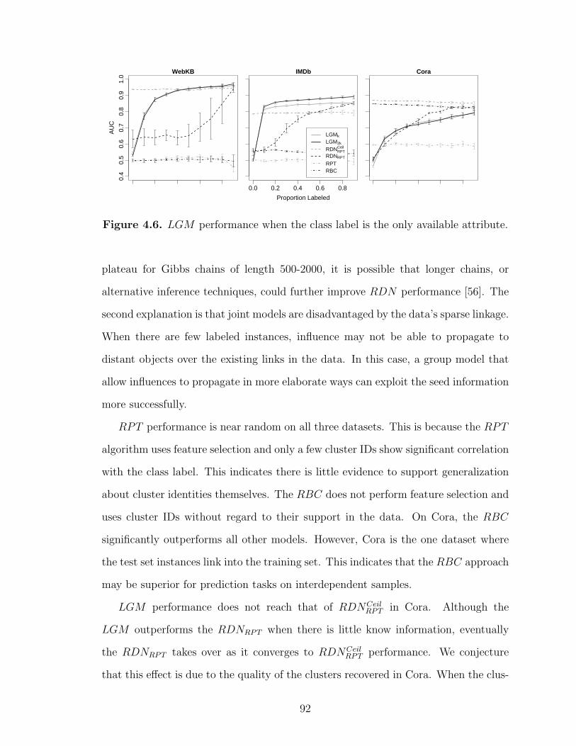
WebKB

0.4

0.5

0.6

0.7

0.8

0.9

1.0

AU

C

IMDb

0.0 0.2 0.4 0.6 0.8

Proportion Labeled

LGMk

LGM2k

RDNRPTCeil

RDNRPT

RPTRBC

Cora

Figure 4.6. LGM performance when the class label is the only available attribute.

plateau for Gibbs chains of length 500-2000, it is possible that longer chains, or

alternative inference techniques, could further improve RDN performance [56]. The

second explanation is that joint models are disadvantaged by the data’s sparse linkage.

When there are few labeled instances, influence may not be able to propagate to

distant objects over the existing links in the data. In this case, a group model that

allow influences to propagate in more elaborate ways can exploit the seed information

more successfully.

RPT performance is near random on all three datasets. This is because the RPT

algorithm uses feature selection and only a few cluster IDs show significant correlation

with the class label. This indicates there is little evidence to support generalization

about cluster identities themselves. The RBC does not perform feature selection and

uses cluster IDs without regard to their support in the data. On Cora, the RBC

significantly outperforms all other models. However, Cora is the one dataset where

the test set instances link into the training set. This indicates that the RBC approach

may be superior for prediction tasks on interdependent samples.

LGM performance does not reach that of RDNCeilRPT in Cora. Although the

LGM outperforms the RDNRPT when there is little know information, eventually

the RDNRPT takes over as it converges to RDNCeilRPT performance. We conjecture

that this effect is due to the quality of the clusters recovered in Cora. When the clus-

92

ter stopping threshold is more conservative, the clustering algorithm returns fewer,

larger-sized clusters. In this case, the model will be able exploit group structure with

fewer labeled instances. However, when we use a less conservative threshold, the

clustering algorithm returns a greater number of smaller-sized clusters. In this case,

the model has the potential to make more accurate predictions but only when there

is a large number of labeled instances to identify the group attribute values accu-

rately. A technique that allows information to propagate outside the clusters (e.g.,

soft clustering) may be more robust in this situation.

Figure 4.7 shows average AUC results for each of the three prediction tasks when

we include attributes in the models. For the WebKB task, we included three page

attributes: school, url-server, url-text ; for IMDb, we included eight movie genre at-

tributes; for Cora, we included three paper attributes: type, year, month. In all three

datasets, the attributes improve LGM performance when there are fewer known la-

bels. This is most pronounced in the IMDb, where LGM achieves ceiling performance

with no class label information, indicating that movie genre is predictive of group at-

tribute. In contrast, the RDNRPT is not able to exploit the attribute information as

fully. In particular, in the WebKB task, the attributes significantly impair RDNRPT

performance. This is due to the RDNRPT feature selection process, which selects bi-

ased page attributes over the pairwise autocorrelation features in this restricted tack.

However, in the other two domains where this is not a problem, the RDNRPT still

does not propagate the attribute information as effectively as the LGM when there

are less than 40% known class labels.

4.3 Related Work

There are two types of relational models relevant to LGMs: those that model

coordinating objects and their properties, and those that model communities and

their properties.

93

WebKB

0.4

0.5

0.6

0.7

0.8

0.9

1.0

AU

C

IMDb

0.0 0.2 0.4 0.6 0.8

Proportion Labeled

LGMk

LGM2k

RDNRPTCeil

RDNRPT

RPTRBC

Cora

Figure 4.7. LGM performance when additional attributes are included.

4.3.1 Modeling Coordinating Objects

Slattery and Mitchell [87] use an approach based on the HITS algorithm [47]

to identify coordinating objects in the data. This approach exploits autocorrelation

dependencies by propagating information through these objects, but it does not gen-

eralize about group properties.

ACORA [80] is a relational learning system that uses novel aggregation function

to capture information in high-dimensional attributes. The ACORA aggregation

functions can be used to model coordinating objects through identifier attributes (e.g.,

object IDs). ACORA’s aggregation functions can also be used to model communities

indirectly. The aggregated features can be used to model the distribution of an

item’s neighboring objects (e.g., a paper’s reference IDs)—and items in the same

community should have similar distributions. Indeed, this approach has achieved

significant gains in classification accuracy compared to RBNs in the Cora domain [80].

However, ACORA features do not generalize about group properties, consequently

this approach must be applied to interdependent samples.

The social networks community provides latent variable models that cluster ob-

jects based on their link structure [77, 36, 94, 44]. These approaches are primarily

used for clustering rather than for prediction. The models use the patterns of re-

lations to identify which roles the objects play in the data. Although these models

94

often incorporate richer representations for the relational link structure (e.g., [94]),

they typically do not incorporate attributes into the model. One exception is the ART

model, where the textual content of email documents is used to moderate pairwise

interactions among individuals and thus refine the process of role discovery to reflect

latent link types [59].

RBNs have been used to cluster the objects in relational datasets [90]. The

approach, which uses latent variables on a subset of object types, will be useful

in situations where the coordinating objects are fixed and known. For example in

the cinematic domain, an RBN with a latent variable on studios could be used to

represent the autocorrelation among movie returns. However, this approach does not

posit group structures. Furthermore, the dependencies among the latent variables, as

with the other dependencies in RBNs, must be structured to be acyclic.

4.3.2 Modeling Communities

Popescul and Ungar [81] cluster relational database tables using standard k-means

clustering algorithms and then use the cluster IDs as features in individual inference

models. This approach has been shown to improve prediction performance, but it

can only be employed in situations where the test set instances link into the clusters

used during training because the features use the identity of the clusters rather than

generalizing over the properties of the groups.

Kubica, Moore, Schneider and Yang [50] use a latent variable model to cluster

objects into groups based on their attribute values and link structure. Their ap-

proach is geared toward clustering data with multiple transactional links (e.g., phone

calls, email) where the link patterns are homogeneous with respect to the groups. In

other words, it is assumed that all groups have the same distribution of intra- and

inter-group linkage. A situation where the patterns of linkage differ among groups is,

however, easy to imagine. For example, consider machine learning papers: Reinforce-

95

ment learning papers tend to cite papers in optimization, operations research, and

theory, but genetic algorithm papers cite primarily other genetic algorithm papers.

Allowing the link probabilities to vary among groups will be important for modeling

group structures in large heterogeneous domains.

4.3.3 Discussion

Consider the case where there are k group attribute values, |C| class values, and

each object has a latent group variable. There is a spectrum of group models ranging

from k = |C| to k =NG. PRMs that model autocorrelation with global parameters,

reason at one end of the spectrum (k= |C|) by implicitly using |C| groups. Techniques

that cluster the data for features to use in individual models (e.g., [81]), reason at

the other end of the spectrum (k = NG) by using the identity of each cluster. The

approach of Kubica et al. [50] uses k = 1 in the sense that it ties the parameters of

intra- and inter-group link probabilities across all groups.

When group size is large, there may be enough data to reason about each group

independently (i.e., use k = NG). For example, once a studio has made a sufficient

number of movies, we can accurately reason about the likely returns of its next movie

independently. However, when group size is small, modeling all groups with the same

distribution (i.e., use k = |C|) will offset the limited data available for each group.

A model that can vary k may be thought of as a backoff model, with the ability to

smooth to the background signal when there is not enough data to accurately estimate

a group’s properties in isolation. LGMs offer a principled framework within which

to explore this spectrum.

One of the primary advantages of LGMs is that influence can propagate between

pairs of objects that are not directly linked but are close in graph space (e.g., in the

same group). In RMNs and RDNs, the features of an object specify its Markov

blanket. This limits influence propagation because features are generally constructed

96

over the attributes of objects one or at most two links away in the data. Influence

can only propagate farther by influencing the probability estimates of attribute values

on each object in a path sequentially. An obvious way to address this issue is to

model the O(N2O) dependencies among all pairs of objects in the data, but dataset

size and sparse link information makes this approach infeasible for most datasets.

PRMs with link uncertainty [54] are the only current models that consider the full

range of dependencies and their influence on observed attributes. Because LGMs can

aggregate influence over an extended local neighborhood, they are a natural way to

expand current representations while limiting the number of dependencies to model.

4.4 Conclusion

In this chapter, we presented latent group models, a PRM extension that mod-

els attribute and link structure jointly, using latent groups to improve reasoning in

relational domains. To date, work on statistical relational models focused primarily

on models of attributes conditioned on the link structure (e.g., [89]), or on models of

link structure conditioned on the attributes (e.g., [54]). Our initial investigation has

shown that modeling the interaction among links and attributes can improve model

generalization when there is natural clustering in the data.

Latent group models are a natural means to model the attribute and link struc-

ture simultaneously. The groups decouple the link and attribute structure, thereby

offering a way to learn joint models tractably. Our analysis has shown that group

models outperform other collective models when there is little information to seed

inference. This is likely because a smaller amount of information is needed to infer

group properties than is needed to propagate information throughout sparse relational

graphs. This suggests active inference as an interesting new research direction—where

techniques choose which instances to label based on estimated improvement to the

collective predictions.

97

Latent group models extend the manner in which collective models exploit au-

tocorrelation to improve model performance. One of the reasons collective inference

approaches work is that the class labels are at the “right” level of abstraction—they

summarize the attribute information that is relevant to related objects [42]. Group

models also summarize the information but at higher level of abstraction (i.e., group

membership and properties). Positing the existence of groups decouples the search

space into a set of biased abstractions and could be considered a form of predicate

invention [88]. This allows the model to consider a wider range of dependencies to

reduce bias while limiting potential increases in variance. Indeed, the results we re-

port for LGMs using only the class labels and the link information achieve nearly the

same level of performance reported by relational models in the recent literature.

98

CHAPTER 5

BIAS/VARIANCE ANALYSIS

Our evaluation of model performance herein has demonstrated that each model

reacts differently to various relational data characteristics—graph structure, level

of autocorrelation, and the amount of seed information available for inference. To

quantify the effects of data characteristics on performance more formally, we outline

a bias/variance framework for relational datasets.

Bias/variance analysis is a useful tool for investigating the performance of ma-

chine learning algorithms. Conventional analysis decomposes loss into errors due to

aspects of the learning process, but in relational and network applications, the infer-

ence process introduces an additional source of error. Collective inference techniques

introduce additional error both through the use of approximate inference algorithms

and through variation in the availability of test set information. To date, the impact

of inference error on model performance has not been investigated. In this chapter,

we outline a new bias/variance framework that decomposes loss into errors due to

both the learning and inference processes. We evaluate performance of a number of

relational models on synthetic data and utilize the framework to investigate hypothe-

ses regarding the mechanisms behind poor model performance (e.g., identifiability

problems increase RDN inference variance). With this understanding, we propose a

number of algorithmic modifications to explore to improve model performance.

99

5.1 Conventional Approach

Bias/variance analysis [25, 16] has been used for a number of years to investigate

the mechanisms behind model performance. This analysis is based on the fundamen-

tal understanding that prediction error has three components (bias, variance, and

noise) and that there is a tradeoff between bias and variance when learning statistical

models. Searching over a larger model space, to estimate a more complex model, can

decrease bias but often increases variance. On the other hand, very simple models can

sometimes outperform complex models due to decreased variance, albeit with higher

bias (e.g., [37]).

Conventional bias/variance analysis decomposes loss into errors due to aspects of

learning procedures. Loss is decomposed into three factors: bias, variance and noise.

In the traditional decomposition, bias and variance measure estimation errors in the

learning technique. For example, the Naive Bayes classifier typically has high bias

due to the assumption of independence among features, but low variance due to the

use of a large sample (i.e., entire training set) to estimate the conditional probability

distribution for each feature [17].

The assumption underlying the conventional decomposition is that there is no

variation in model predictions due to (1) the inference process, and (2) the available

information in the test set. Classification of relational data often violates these as-

sumptions when collective inference techniques are used. Collective inference often

requires the use of approximate inference techniques, which can introduce variation

in model predictions for a single instance. For example, final predictions for an in-

stance may depend on the initial (random) start state used during inference, thus

multiple runs of inference may result in different predictions. In addition, relational

models are often applied to classify a partially labeled test set, where the known class

labels serve to seed the collective inference process. Current methods for evaluating

relational learning techniques typically assume that labeling different nodes in the

100

test set have equivalent impact. However, the heterogeneity of the relational graph

may allow some instances to have more of an impact on neighbor predictions than

others—thus, which instances are labeled in the test set may cause additional vari-

ation in the predictions. Finally, relational models are generally learned on a fully

labeled training set (i.e., the class labels of all neighbors are known), but then applied

to an unlabeled, or partially labeled, test set. This mismatch between training and

test set information may impact the final model predictions.

To date, the impact of inference error on model performance has not been inves-

tigated. In this chapter, we propose a new bias/variance framework that decomposes

marginal squared-loss error into components of both the learning and inference pro-

cesses. We evaluate the performance of a number of relational models on synthetic

data and use the framework to understand the reasons for poor model performance.

Each of the models exhibits a different relationship between error and dataset char-

acteristics. For example, RMNs have higher inference bias in densely connected net-

works; RDNs have higher inference variance when there is little information to seed

the inference process; LGMs have higher learning bias when the underlying group

structure is difficult to identify from the network structure. Using this understanding,

we propose a number of algorithmic modifications to improve model performance.

5.2 Relational framework

In conventional bias/variance analysis, loss is decomposed into three factors: bias,

variance and noise [25, 16]. Given an example x, a model that produces a prediction

f(x) = y, and a true value for x of t, squared loss is defined as: L(t, y) = (t − y)2.

The expected loss for an example x can be decomposed into bias, variance, and

noise components. Here the expectation is over training sets D—the expected loss is

measured with respect to the variation in predictions for x when the model is learned

on different training sets: ED,t[L(t, y)] = B(x) + V (x) + N(x).

101

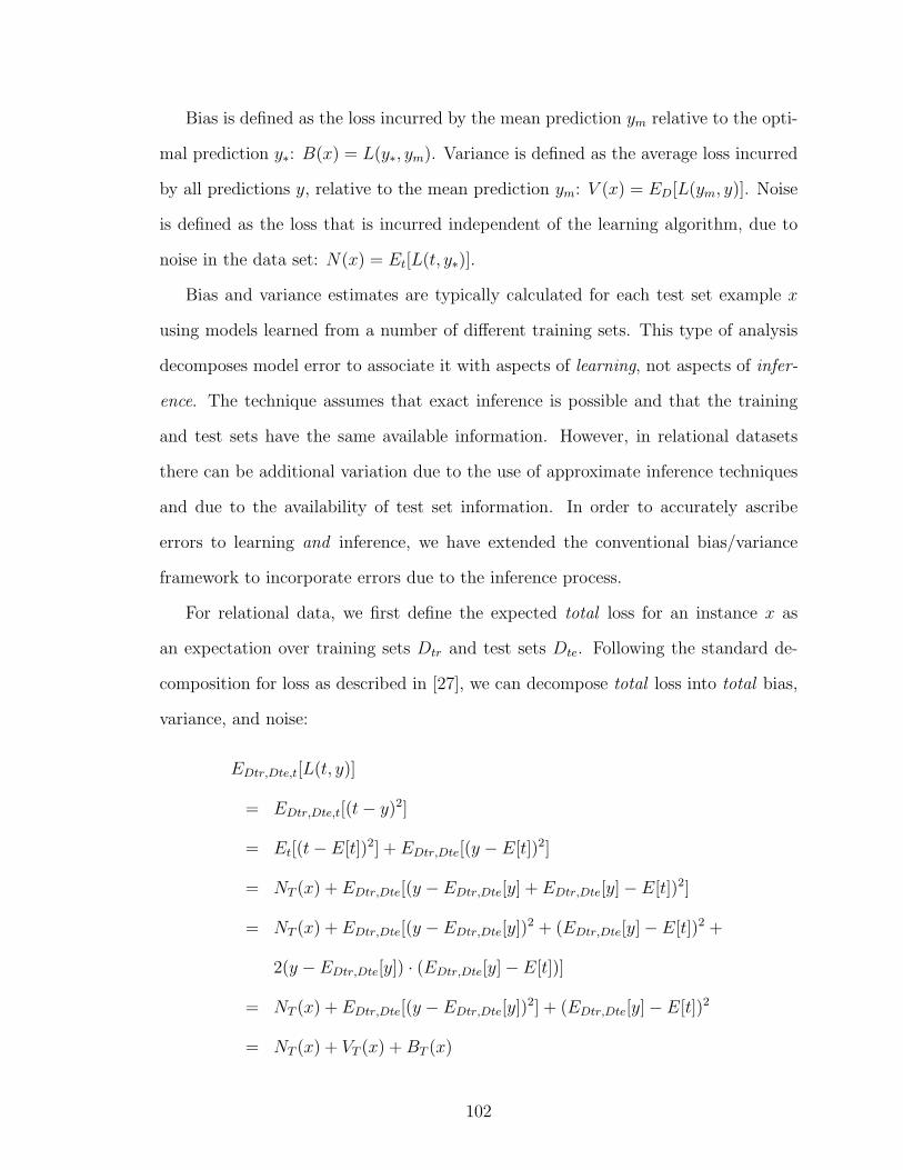
Bias is defined as the loss incurred by the mean prediction ym relative to the opti-

mal prediction y∗: B(x) = L(y∗, ym). Variance is defined as the average loss incurred

by all predictions y, relative to the mean prediction ym: V (x) = ED[L(ym, y)]. Noise

is defined as the loss that is incurred independent of the learning algorithm, due to

noise in the data set: N(x) = Et[L(t, y∗)].

Bias and variance estimates are typically calculated for each test set example x

using models learned from a number of different training sets. This type of analysis

decomposes model error to associate it with aspects of learning, not aspects of infer-

ence. The technique assumes that exact inference is possible and that the training

and test sets have the same available information. However, in relational datasets

there can be additional variation due to the use of approximate inference techniques

and due to the availability of test set information. In order to accurately ascribe

errors to learning and inference, we have extended the conventional bias/variance

framework to incorporate errors due to the inference process.

For relational data, we first define the expected total loss for an instance x as

an expectation over training sets Dtr and test sets Dte. Following the standard de-

composition for loss as described in [27], we can decompose total loss into total bias,

variance, and noise:

EDtr,Dte,t[L(t, y)]

= EDtr,Dte,t[(t− y)2]

= Et[(t− E[t])2] + EDtr,Dte[(y − E[t])2]

= NT (x) + EDtr,Dte[(y − EDtr,Dte[y] + EDtr,Dte[y]− E[t])2]

= NT (x) + EDtr,Dte[(y − EDtr,Dte[y])2 + (EDtr,Dte[y]− E[t])2 +

2(y − EDtr,Dte[y]) · (EDtr,Dte[y]− E[t])]

= NT (x) + EDtr,Dte[(y − EDtr,Dte[y])2] + (EDtr,Dte[y]− E[t])2

= NT (x) + VT (x) + BT (x)

102

In this decomposition the total bias BT (x), and total variance VT (x) are calculated

with respect to variation in model predictions due to both the learning and inference

algorithms.

Then we define the learning loss as an expectation over training sets Dtr alone,

using a fully labeled test set for inference. For example, when predicting the class

label for instance xi, the model is allowed to use the class labels (and attributes) of

all other instances in the dataset (X − xi). This enables the application of exact

inference techniques and ensures that the test set information most closely matches

the information used during learning. Note that this part of the analysis mirrors the

conventional approach to bias/variance decomposition, isolating the errors due to the

learning process. For this reason, we will refer to the components as learning bias,

variance, and noise:

EDtr,t[L(t, y)]

= EDtr,t[(t− y)2]

= Et[(t− E[t])2] + EDtr[(y − E[t])2]

= NL(x) + EDtr[(y − EDtr[y] + EDtr[y]− E[t])2]

= NL(x) + EDtr[(y − EDtr[y])2 + (EDtr[y]− E[t])2 +

2(y − EDtr[y]) · (EDtr[y]− E[t])]

= NL(x) + EDtr[(y − EDtr[y])2] + (EDtr[y]− E[t])2

= NL(x) + VL(x) + BL(x)

Once we have measured the total and learning bias/variance, we can define infer-

ence bias/variance as the difference between the total error and the error due to the

learning process alone:

BI(x) = BT (x)−BL(x)

VI(x) = VT (x)− VL(x)

103

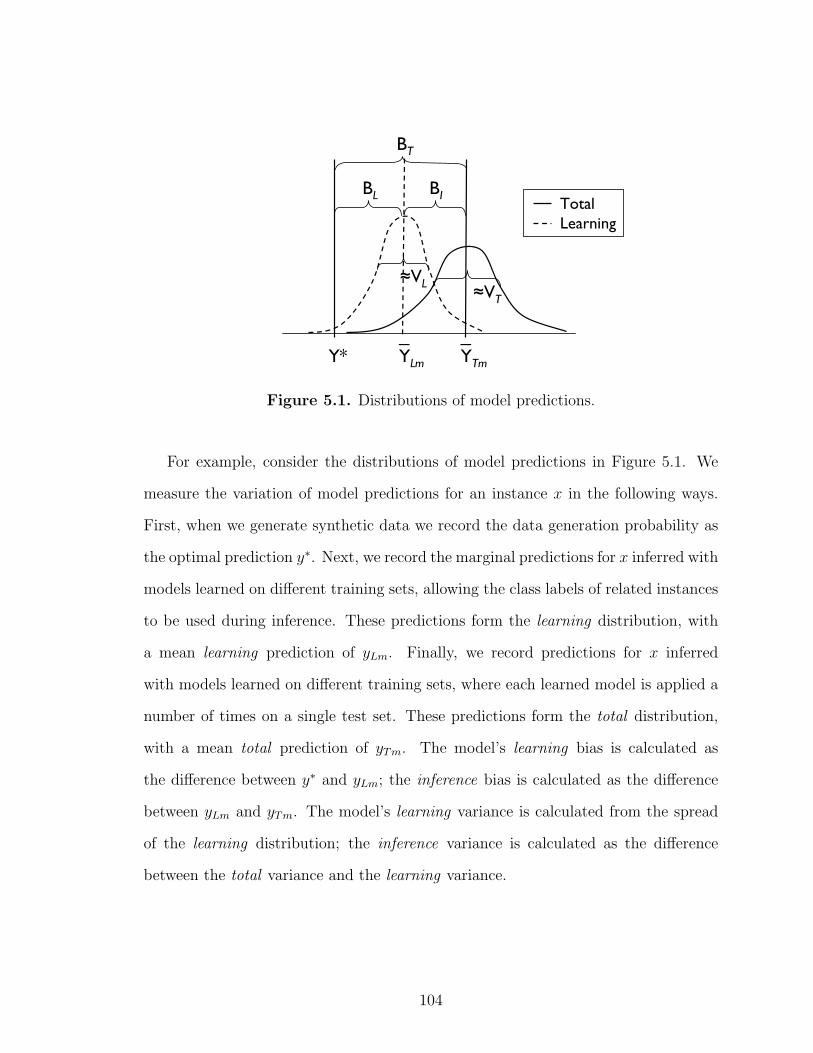
18/13

Y* YTm_

YLm_

BT

BIBL

≈VT≈VL

TotalLearning

Figure 5.1. Distributions of model predictions.

For example, consider the distributions of model predictions in Figure 5.1. We

measure the variation of model predictions for an instance x in the following ways.

First, when we generate synthetic data we record the data generation probability as

the optimal prediction y∗. Next, we record the marginal predictions for x inferred with

models learned on different training sets, allowing the class labels of related instances

to be used during inference. These predictions form the learning distribution, with

a mean learning prediction of yLm. Finally, we record predictions for x inferred

with models learned on different training sets, where each learned model is applied a

number of times on a single test set. These predictions form the total distribution,

with a mean total prediction of yTm. The model’s learning bias is calculated as

the difference between y∗ and yLm; the inference bias is calculated as the difference

between yLm and yTm. The model’s learning variance is calculated from the spread

of the learning distribution; the inference variance is calculated as the difference

between the total variance and the learning variance.

104

5.3 Experimental Evaluation

To explore the effects of relational graph and attribute structure on model perfor-

mance, we used the RDN and LGM data generation procedures described in chap-

ters 3 and 4. The details of the synthetic data generation procedures are outlined in

appendices A.1.1 and A.1.2.

Our experiments evaluate model performance in a prediction context, where only

a single attribute is unobserved in the test set. We generated disjoint training and

test sets and learned models to predict X1 using the intrinsic attributes of the object

(X2, X3, X4) as well as the class label and the attributes of directly related objects

(X1, X2, X3, X4). During inference we varied the number of known class labels in

the test set, measuring performance on the remaining unlabeled instances. To eval-

uate model performance, we measured squared loss and decomposed it into bias and

variance components for each model.

To measure, and decompose, the expected loss over training and test sets, we used

the following procedure:

1. For each outer trial i = [1, 5]:

(a) Generate test set.

(b) For each learning trial j = [1, 5]:

i. Generate training set, record optimal predictions.

ii. Learn model of X1 on the training set.

iii. Infer marginal probabilities for test set with fully labeled test data

(i.e., X− Xi), record learning predictions.

iv. For each inference trial k = [1, 5] and proportion labeled p= [0.0, 0.3, 0.6]:

A. Randomly label p% of test set.

B. Infer marginal probabilities for unlabeled test instances, record

total predictions.

105

C. Measure squared loss.

(c) Calculate learning bias and variance from distributions of learning predic-

tions.

(d) Calculate total bias and variance from distributions of total predictions.

2. Calculate average model loss.

3. Calculate average learning bias and variance.

4. Calculate average total bias and variance.

5.3.1 RDN Analysis

The first set of bias/variance experiments evaluates the data and models from

Section 3.3.1. More specifically, we compare the performance of three models: RDN ,

RMN , and RMNSel.

Figure 5.2 graphs the squared loss decomposition for each model on data generated

with an RDNRPT . Again, we vary the level of autocorrelation and the proportion

of labeled instances in the test set. The first column graphs overall loss; the second

column graphs total and learning bias; the third column graphs total and learning

variance. Inference bias (variance) is calculated as the difference between total bias

(variance) and learning bias (variance).

On the low autocorrelation data (row a), both the RMN and the RMNSel have

higher loss than the RDN . This is primarily due to high learning bias of the RMN

and RMNSel. Recall that we had hypothesized that since the data were generated

with an RDNRPT , an RMN would not be able to represent the data dependencies

as well as an RDN when autocorrelation is less extreme (due to incompatible feature

spaces). The high learning bias for RMNs supports this hypothesis. In contrast,

the RDN has very low learning bias across all experiments—which is to be expected

because the data were generated with an RDN .

106

0.0 0.1 0.2 0.3 0.4 0.5 0.6

0.0

0.1

0.2

0.3

0.4

Proportion Labeled

Squ

ared

Los

s

Loss

Squ

ared

Los

s

RDNRMNRMNSel

0.0 0.1 0.2 0.3 0.4 0.5 0.6

0.00

0.05

0.10

0.15

0.20

Proportion Labeled

Squ

ared

Los

s

Bias(a) Autocorrelation=0.25

0.0 0.1 0.2 0.3 0.4 0.5 0.6

0.00

0.05

0.10

0.15

Proportion Labeled

Squ

ared

Los

s

Variance

RDN−totalRDN−learnRMN−totalRMN−learnRMNSel−totalRMNSel−learn

0.0 0.1 0.2 0.3 0.4 0.5 0.6

0.0

0.1

0.2

0.3

0.4

Proportion Labeled

Squ

ared

Los

s

Loss

Squ

ared

Los

s

0.0 0.1 0.2 0.3 0.4 0.5 0.6

0.00

0.05

0.10

0.15

0.20

Proportion Labeled

Squ

ared

Los

s

Bias(b) Autocorrelation=0.50

0.0 0.1 0.2 0.3 0.4 0.5 0.6

0.00

0.05

0.10

0.15

Proportion Labeled

Squ

ared

Los

s

Variance

0.0 0.1 0.2 0.3 0.4 0.5 0.6

0.0

0.1

0.2

0.3

0.4

Proportion Labeled

Squ

ared

Los

s

Loss

Squ

ared

Los

s

0.0 0.1 0.2 0.3 0.4 0.5 0.6

0.00

0.05

0.10

0.15

0.20

Proportion Labeled

Squ

ared

Los

s

Bias(c) Autocorrelation=0.75

0.0 0.1 0.2 0.3 0.4 0.5 0.6

0.00

0.05

0.10

0.15

Proportion Labeled

Squ

ared

Los

s

Variance

Figure 5.2. Bias/variance analysis on RDNRPT synthetic data.

107

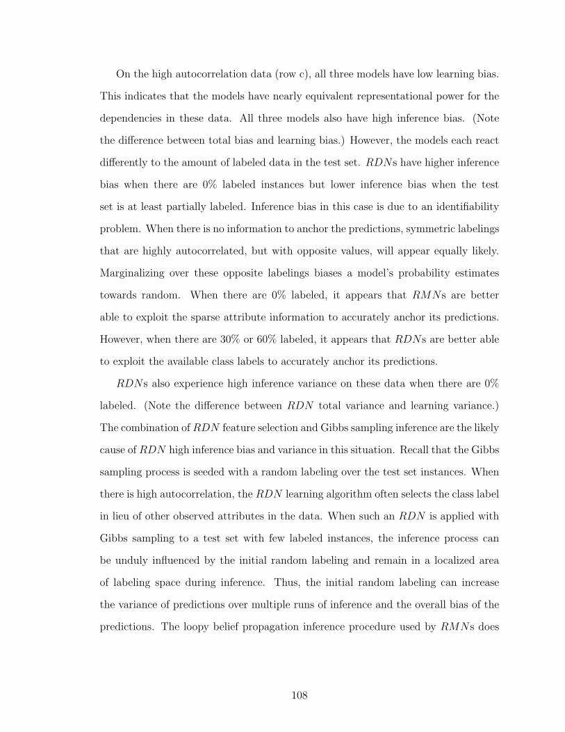
On the high autocorrelation data (row c), all three models have low learning bias.

This indicates that the models have nearly equivalent representational power for the

dependencies in these data. All three models also have high inference bias. (Note

the difference between total bias and learning bias.) However, the models each react

differently to the amount of labeled data in the test set. RDNs have higher inference

bias when there are 0% labeled instances but lower inference bias when the test

set is at least partially labeled. Inference bias in this case is due to an identifiability

problem. When there is no information to anchor the predictions, symmetric labelings

that are highly autocorrelated, but with opposite values, will appear equally likely.

Marginalizing over these opposite labelings biases a model’s probability estimates

towards random. When there are 0% labeled, it appears that RMNs are better

able to exploit the sparse attribute information to accurately anchor its predictions.

However, when there are 30% or 60% labeled, it appears that RDNs are better able

to exploit the available class labels to accurately anchor its predictions.

RDNs also experience high inference variance on these data when there are 0%

labeled. (Note the difference between RDN total variance and learning variance.)

The combination of RDN feature selection and Gibbs sampling inference are the likely

cause of RDN high inference bias and variance in this situation. Recall that the Gibbs

sampling process is seeded with a random labeling over the test set instances. When

there is high autocorrelation, the RDN learning algorithm often selects the class label

in lieu of other observed attributes in the data. When such an RDN is applied with

Gibbs sampling to a test set with few labeled instances, the inference process can

be unduly influenced by the initial random labeling and remain in a localized area

of labeling space during inference. Thus, the initial random labeling can increase

the variance of predictions over multiple runs of inference and the overall bias of the

predictions. The loopy belief propagation inference procedure used by RMNs does

108

not use an initial random labeling, and consequently it is not as susceptible to this

problem.

On the earlier experiments in Section 3.3.1, RMNSel significantly outperformed

the RMN on data with low and medium autocorrelation. However, when we measure

squared-loss the RMN has significantly lower loss than the RMNSel on data with

medium levels of autocorrelation. On these data, the RMNSel has higher learning

bias than the RMN , which indicates that learning bias can skew probability estimates

in RMNs without necessarily affecting the overall ranking of the estimates.

Figure 5.3 graphs the squared loss decomposition for each model on data generated

with an RDNRBC . Recall that the RMN feature space is more comparable to data

generated by an RDNRBC because both models represent the dependencies among all

neighbor values individually, instead of aggregating related values into a single value

before modeling dependencies, as the RDNRPT does.

As expected, because the features spaces are more comparable, RMN learning

bias is similar to RDN on all but the low autocorrelation data. It is this difference

in learning bias that accounts for the RMN ’s inferior performance on the low auto-

correlation data. This indicates that minor incompatibilities in representation have

more effect in noisy data.

On the medium autocorrelation data (row b), RDNs have higher squared loss

compared to the RMN . However, our previous experiments in Section 3.3.1 showed

RDNs have higher AUC on the same data. This indicates that the RDNs produce

better rankings of the inferred probability estimates but the estimates themselves

are not as accurate. The squared-loss decomposition shows that the inaccuracies are

due to high inference variance. The RDNRBC has higher inference variance on the

medium autocorrelation data than on the high autocorrelation data, particularly on

the trials with 0% labeled instances. This indicates that a small amount of informa-

tion may unduly influence the RDNRBC which models each of an object’s neighbors

109

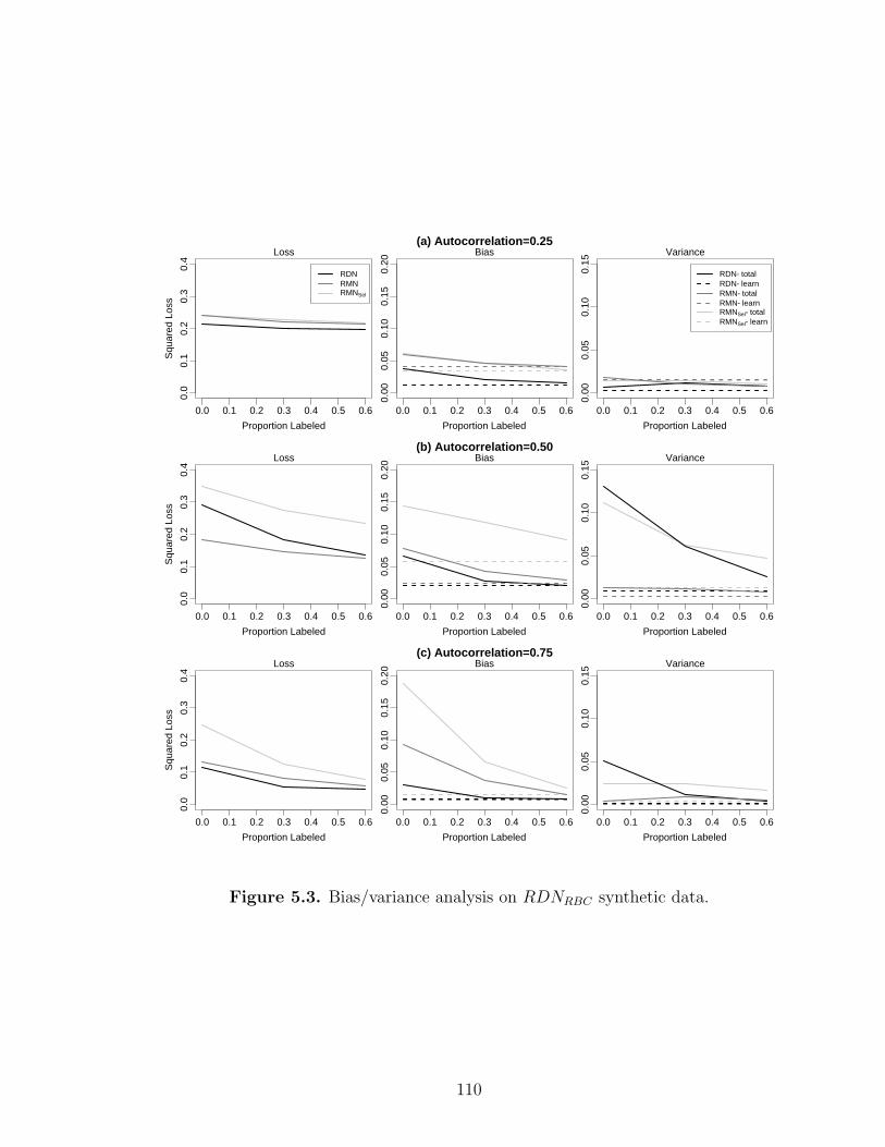
0.0 0.1 0.2 0.3 0.4 0.5 0.6

0.0

0.1

0.2

0.3

0.4

Proportion Labeled

Squ

ared

Los

s

Loss

Squ

ared

Los

s

RDNRMNRMNSel

0.0 0.1 0.2 0.3 0.4 0.5 0.6

0.00

0.05

0.10

0.15

0.20

Proportion Labeled

Squ

ared

Los

s

Bias(a) Autocorrelation=0.25

0.0 0.1 0.2 0.3 0.4 0.5 0.6

0.00

0.05

0.10

0.15

Proportion Labeled

Squ

ared

Los

s

Variance

RDN−totalRDN−learnRMN−totalRMN−learnRMNSel−totalRMNSel−learn

0.0 0.1 0.2 0.3 0.4 0.5 0.6

0.0

0.1

0.2

0.3

0.4

Proportion Labeled

Squ

ared

Los

s

Loss

Squ

ared

Los

s

0.0 0.1 0.2 0.3 0.4 0.5 0.6

0.00

0.05

0.10

0.15

0.20

Proportion Labeled

Squ

ared

Los

s

Bias(b) Autocorrelation=0.50

0.0 0.1 0.2 0.3 0.4 0.5 0.6

0.00

0.05

0.10

0.15

Proportion Labeled

Squ

ared

Los

s

Variance

0.0 0.1 0.2 0.3 0.4 0.5 0.6

0.0

0.1

0.2

0.3

0.4

Proportion Labeled

Squ

ared

Los

s

Loss

Squ

ared

Los

s

0.0 0.1 0.2 0.3 0.4 0.5 0.6

0.00

0.05

0.10

0.15

0.20

Proportion Labeled

Squ

ared

Los

s

Bias(c) Autocorrelation=0.75

0.0 0.1 0.2 0.3 0.4 0.5 0.6

0.00

0.05

0.10

0.15

Proportion Labeled

Squ

ared

Los

s

Variance

Figure 5.3. Bias/variance analysis on RDNRBC synthetic data.

110

individually. On the low autocorrelation data, there is not enough information in the

neighbor attributes to drive the model to extreme labelings; on the high autocorrela-

tion data, there is enough information to keep the inference process from converging

to such extremes.

On the high autocorrelation data (row c), where identifiability issues are more of

a problem, RDN performance is somewhat better than RMNs. This suggests that

RDN inference variance has less of an effect than RMN inference bias on perfor-

mance. This may indicate that marginalizing over the set of labelings that are easily

reached through finite Gibbs sampling is more effective than marginalizing over all

possible labelings.

5.3.2 LGM Analysis

The second set of bias/variance experiments evaluates the data and models from

Section 4.2.1. More specifically, we compare the performance of four models: LGM ,

RDN , RMN , and RDNGrp.

Figure 5.4 graphs performance on the four different types of LGM data, with

small/large group sizes and high/low linkage. Again, we graph the squared loss

decomposition for each model as the level of test-set labeling is varied. We investigated

performance for different levels of autocorrelation, however we only report results for

medium autocorrelation because varying autocorrelation does not alter the relative

performance of the models—lower levels of autocorrelation weaken the effects, higher

levels strength the effects.

When group size is small and linkage is high (row b), the LGM is outperformed

by the RDN when the test data are at least partially labeled. The bias/variance

decomposition shows that poor LGM performance is due to high learning bias. This

is due to the LGM algorithm’s inability to identify the latent group structure when

group size is small and linkage is high. When density of linkage between groups is

111

0.0 0.1 0.2 0.3 0.4 0.5 0.6

0.10

0.15

0.20

0.25

Proportion Labeled

Squ

ared

Los

s

Loss

Squ

ared

Los

sLGMRDNRMNRDNGrp

0.0 0.1 0.2 0.3 0.4 0.5 0.6

0.00

0.05

0.10

0.15

Proportion Labeled

Squ

ared

Los

s

Bias(a) Group size=small, linkage=low

0.0 0.1 0.2 0.3 0.4 0.5 0.6

0.00

0.02

0.04

0.06

0.08

Proportion Labeled

Squ

ared

Los

s

Variance

LGM−totalLGM−learnRDN−totalRDN−learnRMN−totalRMN−learnRDNGrp−totalRDNGrp−learn

0.0 0.1 0.2 0.3 0.4 0.5 0.6

0.10

0.15

0.20

0.25

Proportion Labeled

Squ

ared

Los

s

Loss

Squ

ared

Los

s

0.0 0.1 0.2 0.3 0.4 0.5 0.6

0.00

0.05

0.10

0.15

Proportion Labeled

Squ

ared

Los

s

Bias(b) Group size=small, linkage=high

0.0 0.1 0.2 0.3 0.4 0.5 0.6

0.00

0.02

0.04

0.06

0.08

Proportion Labeled

Squ

ared

Los

s

Variance

0.0 0.1 0.2 0.3 0.4 0.5 0.6

0.10

0.15

0.20

0.25

Proportion Labeled

Squ

ared

Los

s

Loss

Squ

ared

Los

s

0.0 0.1 0.2 0.3 0.4 0.5 0.6

0.00

0.05

0.10

0.15

Proportion Labeled

Squ

ared

Los

s

Bias(c) Group size=large, linkage=low

0.0 0.1 0.2 0.3 0.4 0.5 0.6

0.00

0.02

0.04

0.06

0.08

Proportion Labeled

Squ

ared

Los

sVariance

0.0 0.1 0.2 0.3 0.4 0.5 0.6

0.10

0.15

0.20

0.25

Proportion Labeled

Squ

ared

Los

s

Loss

Squ

ared

Los

s

0.0 0.1 0.2 0.3 0.4 0.5 0.6

0.00

0.05

0.10

0.15

Proportion Labeled

Squ

ared

Los

s

Bias(d) Group size=large, linkage=high

0.0 0.1 0.2 0.3 0.4 0.5 0.6

0.00

0.02

0.04

0.06

0.08

Proportion Labeled

Squ

ared

Los

s

Variance

Figure 5.4. Bias/variance analysis on LGM synthetic data.

112

relatively high compared to group size it is difficult for the LGM spectral clustering

algorithm to correctly identify the fine grained underlying group structure, and this in

turn will bias the learned model. When we allow LGMs to utilize the true underlying

group structure, this bias disappears.

When group size is large (row c and d), the LGM significantly outperforms the

RDN . The bias/variance decomposition shows that poor RDN performance is due

to bias and variance in the inference process. This indicates that LGMs are less

susceptible to identifiability problems than other PRMs when the data exhibit clus-

tering. LGMs use link structure to exploit information from more distant but related

parts of the data graph and this additional information may be enough to anchor the

predictions in a sparsely labeled dataset. Notice that the RDN does not suffer from

high inference variance in data with small groups. This suggests that the Gibbs sam-

pling is less likely to be influenced by the initial labeling when the underlying group

structures are small—larger groups may prevent the Gibbs chain from mixing well.

When group size is large, both the LGM and the RDN significantly outperform

the RMN , provided the test set is at least partially labeled. In these cases, the

bias/variance decompositions show that poor RMN performance is due to high in-

ference bias. In fact, RMN total bias is similar across all four types of data, but

RMN learning bias is lower when group size is large. This indicates that RMN in-

ference bias is always high, perhaps due to a bias in loopy belief propagation when it

is run in a densely connected network. This could also be a result of the RMN algo-

rithm learning skewed clique weights when the network has large underlying groups.

When these weights are applied with loopy belief propagation to collectively infer

the labels throughout the test set, the inference process may converge to extreme

labelings when the graph is very “loopy” (i.e., densely connected). We experimented

with a wide range of priors to limit to the impact of weight overfitting but the effect

remained consistent.

113

On the previous experiments in Section 4.2.1, we showed the RDN always out-

performs the RDNGrp. The bias/variance decompositions show that poor RDNGrp

performance is due to extremely high inference variance. This indicates that the

additional group links make the Gibbs sampling inference procedure even more sus-

ceptible to variance due to the initial labelings by preventing the Gibbs chain from

mixing well. In addition, the RDNGrp has much higher variance than the RDN in

the data with small groups (row a and b). When the LGM learning procedure is

biased, the identified groups (and thus links added to RDNGrp) are less accurate.

These “noisy” links allow the Gibbs initial labeling to influence a wider relational

neighborhood and make it more likely that the RDNGrp inference procedure will only

explore states near the initial labeling.

5.4 Conclusion

This chapter presents a new bias/variance framework that decomposes squared-

loss error into aspects of both the learning and inference processes. To date, work

on relational models focused primarily on the development of models and algorithms

rather than the analysis of mechanisms behind model performance. In particular, the

impact of collective inference techniques applied to graphs of various structure has

not been explored. This work has demonstrated the effects of graph characteristics on

relational model performance, illustrating the situations in which we can expect each

model to perform well. These experiments also help us understand model limitations

and suggest a number of ways to improve the design of relational learning/inference

algorithms.

To improve LGM performance, we need to improve the identification of clusters

when inter-group linkage drowns out a weak intra-group signal. This may be achieved

by the use of alternative clustering techniques in the LGM learning approach, or

114

through the development of a joint learning procedure that clusters for groups while

simultaneously estimating the attribute dependencies in the model.

To improve RDN performance, we need to improve inference when there are few

labeled instances in the test set. This may be achieved through the use of non-random

initial labeling to seed the Gibbs sampling procedure. We have started exploring the

use RPT s, learned on the observed attributes in the data, to predict class labels for

use in the initial Gibbs labeling. Preliminary results indicate that this modification

to the inference procedure reduces RDN loss by 10−15% when there is 0% test

set labeling. Alternatively, we could improve the RDN learning algorithm by using

meta-knowledge about the test set to bias the feature selection process. For example,

if we know that the model will be applied to an unlabeled test set, then we can bias

the selective learning procedure to prefer attributes that will be known with certainty

during the inference process.

Finally, to improve RMN performance, we need to improve inference when con-

nectivity is high, either when there are large clusters or when overall linkage is dense.

This may be achieved through the use of approximate inference techniques other than

loopy belief propagation, or through the use of aggregate features in clique templates

(that summarize cluster information) rather than using redundant pairwise features.

Alternatively, when using pairwise clique templates in a densely connected dataset,

it may be helpful to downsample the links in the graph to reduce inference bias.

115

CHAPTER 6

CONCLUSION

In this chapter, we summarize the contributions of this work and discuss areas for

future work, including model extensions and new directions.

6.1 Contributions

In this thesis, we investigated the connections between autocorrelation and im-

provements in inference due to the use of probabilistic relational models and collective

inference procedures. In particular, we explored the effects of data characteristics and

representation choices on inference accuracy and investigated the mechanisms behind

model performance.

First, we developed RDNs to model the joint distribution of attribute values in re-

lational datasets. RDNs use pseudolikelihood estimation techniques to approximate

the full joint distribution. This approximation enables a relatively simple approach to

parameter estimation and structure learning in relational domains. We demonstrated

the quality of the RDN approximation empirically over a range of data conditions,

showing that if the models are learned from moderate to large datasets, the approx-

imation is accurate. Furthermore, we proved that in the limit as dataset size grows

to infinity, the pseudolikelihood approximation will be an unbiased estimate of the

full joint distribution. RDN learning techniques offer a number of advantages over

comparable PRMs. First, RDN learning is more efficient than both RBNs and

RMNs. Second, RDN learning offers the first tractable means to learn relational au-

116

tocorrelation dependencies. Finally, RDN learning techniques can be used to learn

parsimonious models, which improve inference efficiency and model interpretability.

Next, we developed LGMs to model the joint distribution of attributes and links

in relational datasets. LGMs posit the existence of an underlying group structure to

decouple attribute and link dependencies. The group structures are a low variance

approach to modeling the dependencies among neighboring but unlinked instances

(e.g., transitive relationships [36]), which improves performance by allowing sparse

information to propagate in a more elaborate manner during inference. We demon-

strated empirically that LGMs achieve superior performance over a range of data

conditions, particularly when there is little information to seed the inference process.

Our analysis has explored the use of alternative approaches to representing and

reasoning with relational autocorrelation dependencies. The experiments have demon-

strated a unique property of relational data—there are a number of nearly equivalent

representational choices for relational dependencies that exhibit different performance

characteristics. This indicates that properties other than attribute correlation struc-

ture should be considered when choosing a model for relational datasets. Individual

models (e.g., RPT s and RBCs) represent autocorrelation indirectly through the ob-

served attributes of related instances. This approach will perform well when a single

observed attribute is highly correlated with the class, otherwise it will difficult for

the algorithms to cope with the increased dimensionality during learning. RDNs

represent autocorrelation directly through the class labels of related instances. This

approach will perform well when at least a portion of the test set is labeled—to

anchor the model predictions so the remainder can be easily inferred with collec-

tive inference. LGMs represent autocorrelation indirectly through the properties

of higher-level group structures, which connect members with autocorrelated labels.

This approach will perform well when there is sparse test set information and the

data exhibit clustering or long-range dependencies. In this case, the link structure

117

can be exploited to propagate the sparse information throughout the graph during

collective inference.

Finally, we extended conventional bias/variance analysis to relational domains.

Our bias/variance framework decomposes loss into aspects of both the learning and

the inference processes to account for the additional error due to the use of collective

inference techniques. We compared model performance on synthetic datasets with

different graph characteristics and levels of autocorrelation, varying the availability of

test set information. We demonstrated empirically that collective inference accounts

for a significant portion of model error and that relative model performance varies

significantly across different types of data graphs.

More specifically, our bias/variance analysis has shown the relational data char-

acteristics that can impact model performance. Graph structure, autocorrelation de-

pendencies, and amount of test set labeling, all affect relational model performance.

LGMs are more robust to sparse labeling and perform well when graph clustering is

high. When the underlying groups are small and linkage is low, LGMs experience

high learning bias due to poor cluster identification. RDNs, applied with Gibbs sam-

pling, experience high variance on test data with sparse labeling, but perform well

across a wide range of graph structures. RMNs, applied with loopy belief propaga-

tion, have higher bias on densely connected graphs, but are more robust to sparse test

set labeling. Our analysis has demonstrated the error introduced by the use of collec-

tive inference techniques and how that error varies across models and datasets. This

suggests a number of directions to pursue to improve model performance—either by

incorporating properties of the inference process into learning or through modification

of the inference process based on properties of learning.

Overall, this work provides better models and tools for studying relational datasets—

from the World Wide Web to biological domains; from fraud detection to citation

analysis. Relational data offer unique opportunities to boost model accuracy and

118

improve decision-making quality if the algorithms can learn effectively from the addi-

tional information the relationships provide. A better understanding of probabilistic

relational models, both in theoretical and practical terms, will enable improvements

to the robustness, efficiency, and interpretability of relational models. Through this,

we can extend the range, applicability, and performance gains of all relational models.

6.2 Future Work

There are a number of interesting avenues for future work that modify and extend

the ideas presented in this thesis. We outline immediate areas of future study for each

component first and then discuss farther reaching directions inspired by this thesis.

Our future work on RDNs will investigate modifications to the learning and in-

ference procedures suggested by the bias/variance analysis. Bagging techniques [7]

may be a means of reducing the variance of the RDNRPT Gibbs sampling procedure.

Calibration techniques [96] may improve the RDNRBC probability estimates and re-

duce inference variance. In addition, averaging the estimates of multiple Gibbs chains

may reduce variance while only incurring a moderate increase in computational cost.

Future work will also compare RDNs to Markov logic networks in order to evalu-

ate the performance tradeoffs for using pseudolikelihood approximations in structure

learning techniques for different relational representations.

Our future work on LGMs will also investigate modifications and extensions sug-

gested by the bias/variance analysis. In particular, alternative clustering techniques

or an iterative sequential learning procedure may reduce the LGM learning bias on

data where spectral clustering does not identify the best groupings. Also, to improve

learning bias, we will investigate approaches to estimating the latent group structure

and parameters jointly, perhaps incorporating a hierarchical Dirichlet process [91] to

estimate k. However, a joint learning approach may increase both learning and infer-

ence variance due to the increased size of the model space. In addition, an evaluation

119

in the context of interdependent samples will compare LGMs and the use of identi-

fiers attributes in ACORA [80]. We will evaluate the relative performance gains of

each model when the samples have varying degrees of overlap and explore the utility

of generalizing about group properties in these domains.

There are two directions that we will explore to improve on our initial work with

the bias/variance framework. First, we intend to broaden our analysis to real data sets

and evaluate algorithm modifications in these domains. This will lead towards a full

characterization of the situations in which we can expect relational models to achieve

superior performance. Next, we plan to extend the framework to analyze additional

aspects of model performance. In particular, the analysis of alternative loss functions

(e.g., zero-one) and analysis of errors when estimating the full joint (rather than

marginals), will increase our understanding of model performance over a wider range

of conditions. Also, examining interaction effects between learning and inference

errors may help to inform the design of joint learning and inference procedures, which

could significantly extend the performance gains of relational models.

In broader ranging future work, we plan to continue investigating the behavior of

relational learning techniques, while developing new models and algorithms. A better

understanding of the underlying principles of relational learning will drive the design

of practical models and algorithms for a broad spectrum of tasks, changing the face

of analysis in fields from homeland security to healthcare informatics.

One area of research suggested by the findings in this work, is the interaction be-

tween learning and inference in relational domains. To date, the majority of learning

algorithms have been developed independently of inference algorithms.1 However, we

have shown there are multiple methods of representing the same relational dependen-

cies. The choice of representation can impact performance through different aspects

1The recent work of Wainwright [92] is a notable exception.

120

of learning and inference. This indicates a potential interaction between the choice

of representation for learning and the effectiveness of subsequent inference. A novel

iterative procedure, where measures of inference accuracy and efficiency are used to

bias the learning process, may improve relational model performance and broaden

their applicability. Our bias-variance framework will facilitate the development of

such techniques.

Another area for future work, is the use of underlying group structures to correct

for biases in feature selection in relational data. Prior work has shown that features

of instances with high degree and autocorrelation will have feature score distributions

with increased variance due to lower effective sample sizes [40]. However, our work

on LGMs also indicates that there is a connection between effective sample size and

the underlying groups in the data, particularly when autocorrelation is high. This

connection can be exploited to develop an efficient technique for unbiased feature

selection that is appropriate for all likelihood-based relational models, by explicitly

accounting for group structure in a graph-based resampling technique. This will

enable efficient estimation of the variance of feature scores, which can be used to

calculate the difference between expected and observed variance and then incorporated

into an unbiased model selection framework.

6.3 Conclusion

In conclusion, this thesis has explored the connections between autocorrelation

and improvements in inference due to the use of probabilistic relational models and

collective inference procedures. We have examined autocorrelation as an exemplar

of complex relational dependencies—involving cycles, redundant representations, and

long-ranging correlations. We have shown that there are a number of ways to incorpo-

rate autocorrelation dependencies into PRMs in a tractable manner. The efficiency

gains we obtain with the RDN pseudolikelihood approximation and the LGM decou-

121

pling of attribute and link dependencies will make relational modeling both practical

and feasible in large, relational datasets where current methods are computationally

intensive, if not intractable. We have also explored the performance characteristics

of various relational models, attributing their errors to aspects of the models’ learn-

ing and inference procedures. This is a first step towards a generalization of PRM

characteristics—an investigation of the mechanisms behind performance and a deter-

mination of which situations additional complexity is warranted will lead towards a

better theory of relational learning.

122

APPENDIX

A.1 Datasets

A.1.1 RDN Synthetic Data

Our RDN synthetic datasets are homogeneous data graphs with an autocorrelated

class label and linkage due to an underlying (hidden) group structure. Each object

has four boolean attributes: X1, X2, X3 and X4. We used the following generative

process for a dataset with NO objects and NG groups:

For each object i, 1 ≤ i ≤ NO:

Choose a group gi uniformly from the range [1, NG].

For each object j, 1 ≤ j ≤ NO:

For each object k, j < k ≤ NO:

Choose whether the two objects are linked from p(E|Gj ==

Gk), a Bernoulli probability conditioned on whether the two

objects are in the same group.

For each object i, 1 ≤ i ≤ NO:

Randomly initialize the values of X = X1, X2, X3, X4 from a uni-

form prior distribution.

Update the values of X with 500 iterations of Gibbs sampling using the

specified RDN .

The data generation procedure for X uses a simple RDN where X1 is autocorre-

lated (through objects one link away), X2 depends on X1, and the other two attribute

123

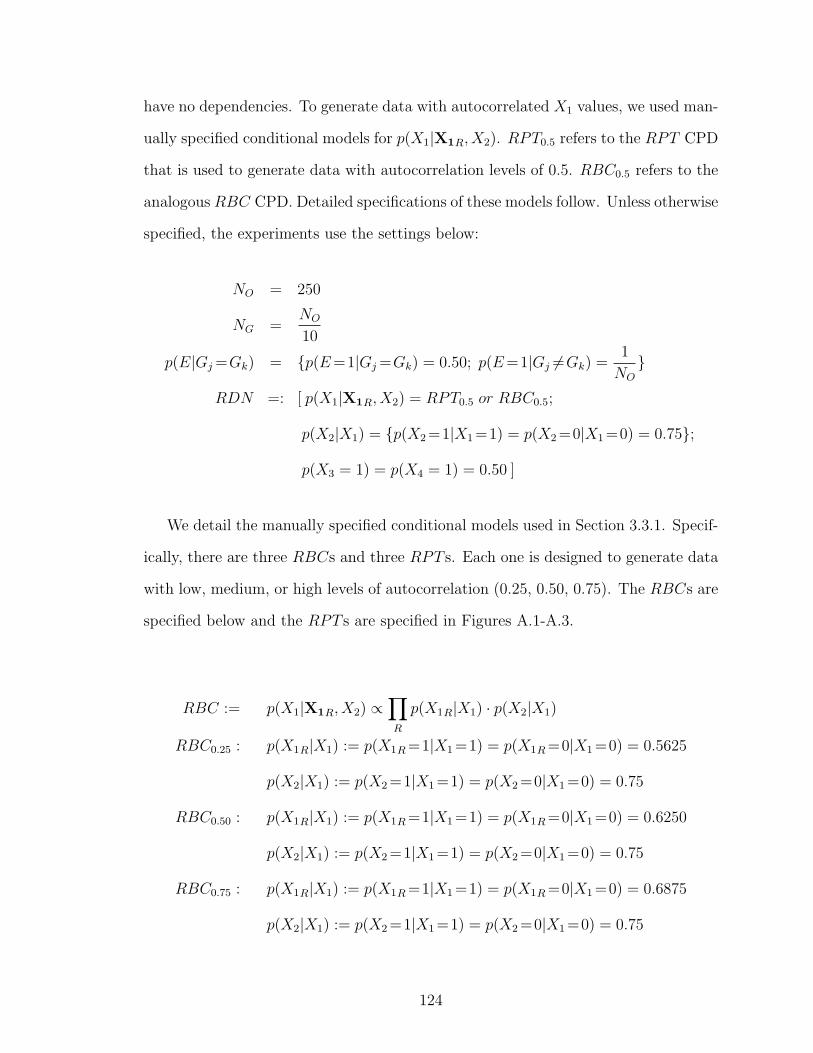
have no dependencies. To generate data with autocorrelated X1 values, we used man-

ually specified conditional models for p(X1|X1R, X2). RPT0.5 refers to the RPT CPD

that is used to generate data with autocorrelation levels of 0.5. RBC0.5 refers to the

analogous RBC CPD. Detailed specifications of these models follow. Unless otherwise

specified, the experiments use the settings below:

NO = 250

NG =NO

10

p(E|Gj =Gk) = p(E =1|Gj =Gk) = 0.50; p(E =1|Gj 6=Gk) =1

NO

RDN =: [ p(X1|X1R, X2) = RPT0.5 or RBC0.5;

p(X2|X1) = p(X2 =1|X1 =1) = p(X2 =0|X1 =0) = 0.75;

p(X3 = 1) = p(X4 = 1) = 0.50 ]

We detail the manually specified conditional models used in Section 3.3.1. Specif-

ically, there are three RBCs and three RPT s. Each one is designed to generate data

with low, medium, or high levels of autocorrelation (0.25, 0.50, 0.75). The RBCs are

specified below and the RPT s are specified in Figures A.1-A.3.

RBC := p(X1|X1R, X2) ∝∏R

p(X1R|X1) · p(X2|X1)

RBC0.25 : p(X1R|X1) := p(X1R =1|X1 =1) = p(X1R =0|X1 =0) = 0.5625

p(X2|X1) := p(X2 =1|X1 =1) = p(X2 =0|X1 =0) = 0.75

RBC0.50 : p(X1R|X1) := p(X1R =1|X1 =1) = p(X1R =0|X1 =0) = 0.6250

p(X2|X1) := p(X2 =1|X1 =1) = p(X2 =0|X1 =0) = 0.75

RBC0.75 : p(X1R|X1) := p(X1R =1|X1 =1) = p(X1R =0|X1 =0) = 0.6875

p(X2|X1) := p(X2 =1|X1 =1) = p(X2 =0|X1 =0) = 0.75

124

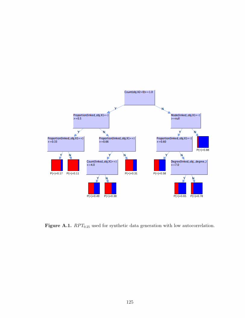
P(+)=0.17 P(+)=0.11

P(+)=0.49 P(+)=0.38

P(+)=0.31 P(+)=0.58

P(+)=0.88

P(+)=0.65 P(+)=0.78

Figure A.1. RPT0.25 used for synthetic data generation with low autocorrelation.

125

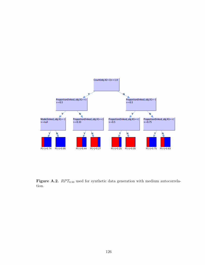
P(+)=0.74 P(+)=0.95 P(+)=0.44 P(+)=0.27 P(+)=0.25 P(+)=0.05 P(+)=0.75 P(+)=0.63

Figure A.2. RPT0.50 used for synthetic data generation with medium autocorrela-tion.

126

P(+)=0.18 P(+)=0.01 P(+)=0.02 P(+)=0.23

P(+)=0.94 P(+)=0.80 P(+)=0.71

P(+)=0.08

P(+)=0.99

P(+)=0.20

Figure A.3. RPT0.75 used for synthetic data generation with high autocorrelationlevels.

127

A.1.2 LGM Synthetic Data

Our LGM synthetic datasets are homogeneous data graphs with autocorrelation

due to an underlying (hidden) group structure. Each object has a group G and four

boolean attributes: X1, X2, X3 and X4. Each group has an associated attribute Xg.

We used the following generative process to generate a dataset with NO objects and

GS average group size:

For each group g, 1 ≤ g ≤ (NG = NO/GS):

Choose a value for group attribute xg from p(Xg).

For each object i, 1 ≤ i ≤ NO:

Choose a group gi uniformly from the range [1, NG].

Choose a class value X1i from p(X1|Xg).

Choose a value for X2i from p(X2|X1).

Choose a value for X3i from p(X3).

Choose a value for X4i from p(X4).

For each object j, 1 ≤ j ≤ NO:

For each object k, j < k ≤ NO:

Choose whether the two objects are linked from p(E|Gj ==Gk).

The procedure uses a simple model where X1 has an autocorrelation level of 0.5, X2

depends on X1, and the other two attributes have no dependencies. Unless otherwise

specified, the experiments use the settings specified below.

128

NO = 250

p(Xg) = p(Xg =1) = 0.50; p(Xg =0) = 0.50

p(X1|Xg) = p(X1 =1|Xg =1)=0.90;

p(X1 =0|Xg =0)=0.90.

p(X2|X1) = p(X2 =1|X1 =1)=0.75;

p(X2 =0|X1 =0)=0.75.

p(X3 =1) = 0.50

p(X4 =1) = 0.50

We generated data with two different groups sizes and levels of linkage:

GS : small = 5; large = 25

Llow|GS = small : p(E =1|Gj =Gk) = 0.50; p(E =1|Gj 6=Gk) = 0.0008.

Lhigh|GS = small : p(E =1|Gj =Gk) = 0.80; p(E =1|Gj 6=Gk) = 0.004.

Llow|GS = large : p(E =1|Gj =Gk) = 0.20; p(E =1|Gj 6=Gk) = 0.0008.

Lhigh|GS = large : p(E =1|Gj =Gk) = 0.30; p(E =1|Gj 6=Gk) = 0.004.

A.1.3 Real World Datasets

Figure A.4 depicts the objects and relations in each real-world dataset.

The first dataset is drawn from Cora, a database of computer science research

papers extracted automatically from the web using machine learning techniques [60].

We selected the set of 4,330 machine-learning papers along with associated authors,

cited papers, and journals. The resulting collection contains approximately 13,000

129

objects and 26,000 links. For classification, we sampled the 1669 papers published

between 1993 and 1998.

On the Cora data, we learned an RDN for seven attributes. Author rank records

ordering in paper authorship (e.g., first author, second author). Paper type records

category information (e.g., PhD thesis, technical report); topic records content in-

formation (e.g., genetic algorithms, reinforcement learning); year and month record

publication dates. Journal name-prefix records the first four title letters (e.g., IEEE,

SIAM); book-role records type information (e.g., workshop, conference).

The second data set (Gene) is a relational data set containing information about

the yeast genome at the gene and the protein level.1 The data set contains information

about 1,243 genes and 1,734 interactions among their associated proteins.

The Gene data contain attributes associated with both objects and links (i.e.,

interactions). We learned an RDN for seven attributes. Gene function records activ-

ities of the proteins encoded by the genes; location records each protein’s localization

in the cell; phenotype records characteristics of individuals with a mutation in the

gene/protein; class records the protein type (e.g., transcription factor, protease); es-

sential records whether the gene is crucial to an organism’s survival. Interaction

expression records the correlation between gene expression patterns for pairs of inter-

acting genes; type records interaction characteristics (e.g., genetic, physical).

The third dataset is drawn from the Internet Movie Database (IMDb).2 We col-

lected a sample of 1,382 movies released in the United States between 1996 and 2001,

with their associated actors, directors, and studios. In total, this sample contains

approximately 42,000 objects and 61,000 links.

On the IMDb data, we learned an RDN for ten discrete attributes. First-movie-

year records the date of the first movie made by a director or studio; has-award records

1See http://www.cs.wisc.edu/∼dpage/kddcup2001/.

2See http:// www.imdb.com.

130

whether a director or actor has won an Academy award; in-US records whether a stu-

dio is located in the US; receipts records whether a movie made more than $2 million

in the opening weekend box office; genre records a movie’s type (e.g., drama, comedy);

hsx-rating records an actor’s value on the Hollywood Stock Exchange (www.hsx.com);

birth-year and gender record demographic information.

Author

Publisher

Paper

Book/Journal

Editor

AuthoredBy AppearsIn

PublishedBy EditedBy

Cites

Studio Actor

Movie

Director

MadeBy ActedIn

Directed

Producer

Produced

Remake

Disclosure Branch

Broker

Regulator Firm

BelongsTo

LocatedAt

WorkedFor

FiledOn

ReportedTo

RegisteredWith

(c)(a)

(d)

Gene

(b)

(e)

Interaction

PageLinkedTo LinkedFrom

Figure A.4. Data schemas for (a) Cora, (b) Gene, (c) IMDb, (d) NASD, and (e)WebKB.

The fourth dataset is from the National Association of Securities Dealers (NASD)

[66]. It is drawn from NASD’s Central Registration Depository (CRD c©) system,

which contains data on approximately 3.4 million securities brokers, 360,000 branches,

25,000 firms, and 550,000 disclosure events. Disclosures record disciplinary informa-

tion on brokers, including information on civil judicial actions, customer complaints,

and termination actions. Our analysis was restricted to small and moderate-size firms

with fewer than 15 brokers, each of whom has an approved NASD registration. We

131

selected a set of approximately 10,000 brokers who were active in the years 1997-2001,

along with 12,000 associated branches, firms, and disclosures.

On the NASD data, we learned an RDN for eleven attributes. Firm size records

the number of employed stockbrokers each year; layoffs records the number of termi-

nations each year. On-watchlist records whether a firm or broker is under heightened

supervision. Broker is-problem and problem-in-past record whether a broker is, or

has been, involved in serious misconduct; has-business records whether a broker owns

a business on the side. Disclosure type and year record category (e.g., customer com-

plaint) and date information regarding disciplinary events (filed on brokers). Region

and area record location information about branches.

The fifth data set was collected by the WebKB Project [12]. The data comprise

3,877 web pages from four computer science departments. The web pages have been

manually labeled with the categories course, faculty, staff, student, research project,

or other. The collection contains approximately 8,000 hyperlinks among the pages.

On the WebKB data, we learned an RDN for four attributes. School records

page location (e.g., Cornell, Washington); label records page type (e.g., student,

course); URL-server records the first portion of the server name following www (e.g.,

cs, engr); URL-text records the name of the first directory in the URL path (e.g.,

UTCS, department).

132

BIBLIOGRAPHY

[1] Anselin, L. Spatial Econometrics: Methods and Models. Kluwer Academic Pub-lisher, The Netherlands, 1998.

[2] Bernstein, A., Clearwater, S., and Provost, F. The relational vector-space modeland industry classification. In Proceedings of the IJCAI-2003 Workshop onLearning Statistical Models from Relational Data (2003), pp. 8–18.

[3] Besag, J. Spatial interaction and the statistical analysis of lattice systems. Jour-nal of the Royal Statistical Society, Series B 36, 2 (1974), 192–236.

[4] Besag, J. Statistical analysis of non-lattice data. The Statistician 24, 3 (1975),179–195.

[5] Blau, H., Immerman, N., and Jensen, D. A visual query language for relationalknowledge discovery. Tech. Rep. 01-28, University of Massachusetts Amherst,Computer Science Department, 2001.

[6] Blei, D., Ng, A., and Jordan, M. Latent Dirichlet allocation. Journal of MachineLearning Research 3 (2003), 993–1022.

[7] Breiman, L. Bagging predictors. Machine Learning 24, 2 (1996), 123–140.

[8] Casella, G., and Berger, R., Eds. Statistical Inference. Druxbury, 2002.

[9] Chakrabarti, S., Dom, B., and Indyk, P. Enhanced hypertext categorizationusing hyperlinks. In Proceedings of the ACM SIGMOD International Conferenceon Management of Data (1998), pp. 307–318.

[10] Comets, F. On consistency of a class of estimators for exponential families ofMarkov random fields on the lattice. The Annals of Statistics 20, 1 (1992),455–468.

[11] Cortes, C., Pregibon, D., and Volinsky, C. Communities of interest. In Pro-ceedings of the 4th International Symposium of Intelligent Data Analysis (2001),pp. 105–114.

[12] Craven, M., DiPasquo, D., Freitag, D., McCallum, A., Mitchell, T., Nigam, K.,and Slattery, S. Learning to extract symbolic knowledge from the World WideWeb. In Proceedings of the 15th National Conference on Artificial Intelligence(1998), pp. 509–516.

133

[13] Cressie, N. Statistics for Spatial Data. John Wiley and Sons, Inc, New York,1993.

[14] Davidson, D. The logical form of action sentences. In The Logic of Decision andAction, N. Rescher, Ed. University of Pittsburgh Press, 1967.

[15] Dempster, A., Laird, N., and Rubin, D. Maximum likelihood from incompletedata via the EM algorithm. Journal of the Royal Statistical Society, Series B39, 1 (1977), 1–38.

[16] Domingos, P. A unified bias-variance decomposition for zero-one and squaredloss. In Proceedings of the 17th National Conference on Artificial Intelligence(2000), pp. 564–569.

[17] Domingos, P., and Pazzani, M. On the optimality of the simple bayesian classifierunder zero-one loss. Machine Learning 29 (1997), 103–130.

[18] Domingos, P., and Richardson, M. Mining the network value of customers. InProceedings of the 7th ACM SIGKDD International Conference on KnowledgeDiscovery and Data Mining (2001), pp. 57–66.

[19] Doreian, P. Network autocorrelation models: Problems and prospects. In Spa-tial Statistics: Past, Present, and Future. Ann Arbor Institute of MathematicalGeography, 1990, ch. Monograph 12, pp. pp. 369–389.

[20] Dzeroski, S., and Lavrac, N., Eds. Relational Data Mining. Springer-Verlag,2001.

[21] Fawcett, T. ROC graphs: Notes and practical considerations for data miningresearchers. Tech. Rep. HPL-2003-4, Hewlett-Packard Labs, 2003.

[22] Fawcett, T., and Provost, F. Adaptive fraud detection. Data Mining and Knowl-edge Discovery 1, 3 (1997), 291–316.

[23] Fayyad, U., Piatetsky-Shapiro, G., Smyth, P., and Uthurusamy, R., Eds. Ad-vances in Knowledge Discovery and Data Mining. M.I.T. Press, 1996.

[24] Flach, P., and Lachiche, N. 1BC: A first-order Bayesian classifier. In Proceedingsof the 9th International Conference on Inductive Logic Programming (1999),pp. 92–103.

[25] Friedman, J. On bias, variance, 0/1-loss, and the curse-of-dimensionality. DataMining and Knowledge Discovery 1, 1 (1997), 55–77.

[26] Friedman, N., Getoor, L., Koller, D., and Pfeffer, A. Learning probabilisticrelational models. In Proceedings of the 16th International Joint Conference onArtificial Intelligence (1999), pp. 1300–1309.

[27] Geman, S., Bienenstock, E., and Doursat, R. Neural networks and thebias/variance dilemma. Neural Computation 4 (1992), 1–58.

134

[28] Geman, S., and Graffine, C. Markov random field image models and their ap-plications to computer vision. In Proceedings of the 1986 International Congressof Mathematicians (1987), pp. 1496–1517.

[29] Getoor, L., Friedman, N., Koller, D., and Pfeffer, A. Learning probabilisticrelational models. In Relational Data Mining. Springer-Verlag, 2001, pp. 307–335.

[30] Getoor, L., Friedman, N., Koller, D., and Taskar, B. Learning probabilisticmodels with link uncertainty. Journal of Machine Learning Research 3 (2002),679–707.

[31] Gidas, B. Consistency of maximum likelihood and pseudolikelihood estimatorsfor Gibbs distributions. In Proceedings of the Workshop on Stochastic DifferentialSystems with Applications in Electrical/Computer Engineering, Control Theory,and Operations Research (1986), pp. 129–145.

[32] Goodman, L. Snowball sampling. Annals of Mathematical Statistics 32 (1961),148–170.

[33] Heckerman, D., Chickering, D., Meek, C., Rounthwaite, R., and Kadie, C. De-pendency networks for inference, collaborative filtering and data visualization.Journal of Machine Learning Research 1 (2000), 49–75.

[34] Heckerman, D., Meek, C., and Koller, D. Probabilistic models for relationaldata. Tech. Rep. MSR-TR-2004-30, Microsoft Research, 2004.

[35] Hill, S., Provost, F., and Volinsky, C. Network-based marketing: Identifyinglikely adopters via consumer networks. Statistical Science 22, 2 (2006).

[36] Hoff, P., Raftery, A., and Handcock, M. Latent space approaches to socialnetwork analysis. Journal of the American Statistical Association 97 (2002),1090–1098.

[37] Holte, R. Very simple classification rules perform well on most commonly useddatatsets. Machine Learning 11 (1993), 63–91.

[38] Jaeger, M. Relational Bayesian networks. In Proceedings of the 13th Conferenceon Uncertainty in Artificial Intelligence (1997), pp. 266–273.

[39] Jensen, D., and Neville, J. Autocorrelation and linkage cause bias in evaluationof relational learners. In Proceedings of the 12th International Conference onInductive Logic Programming (2002), pp. 101–116.

[40] Jensen, D., and Neville, J. Linkage and autocorrelation cause feature selectionbias in relational learning. In Proceedings of the 19th International Conferenceon Machine Learning (2002), pp. 259–266.

135

[41] Jensen, D., and Neville, J. Avoiding bias when aggregating relational data withdegree disparity. In Proceedings of the 20th International Conference on MachineLearning (2003), pp. 274–281.

[42] Jensen, D., Neville, J., and Gallagher, B. Why collective inference improvesrelational classification. In Proceedings of the 10th ACM SIGKDD InternationalConference on Knowledge Discovery and Data Mining (2004), pp. 593–598.

[43] Jordan, M. Graphical models. Statistical Science 19 (2004), 140–155.

[44] Kemp, C., Griffiths, T., and Tenenbaum, J. Discovering latent classes in rela-tional data. Tech. Rep. AI Memo 2004-019, Massachusetts Institute of Technol-ogy, 2004.

[45] Kersting, K. Representational power of probabilistic-logical models: From up-grading to downgrading. In IJCAI-2003 Workshop on Learning Statistical Modelsfrom Relational Data (2003), pp. 61–62.

[46] Kersting, K., and Raedt, L. De. Basic principles of learning Bayesian logicprograms. Tech. Rep. 174, Institute for Computer Science, University of Freiburg,2002.

[47] Kleinberg, J. Authoritative sources in a hyperlinked environment. In Proceedingsof the 9th ACM SIAM Symposium on Discrete Algorithms (1998), pp. 25–27.

[48] Kok, S., and Domingos, P. Learning the structure of Markov logic networks. InProceedings of the 22nd International Conference on Machine Learning (2005),pp. 441–448.

[49] Kramer, S., Lavrac, N., and Flach, P. Propositionalization approaches to rela-tional data mining. In Relational Data Mining. Springer-Verlag, 2001, pp. 262–291.

[50] Kubica, J., Moore, A., Schneider, J., and Yang, Y. Stochastic link and groupdetection. In Proceedings of AAAI/IAAI 2002 (2002), pp. 798–806.

[51] Lafferty, J., McCallum, A., and Pereira, F. Conditional random fields: Proba-bilistic models for segmenting and labeling sequence data. In Proceedings of the18th International Conference on Machine Learning (2001), pp. 282–289.

[52] Lauritzen, S., and Sheehan, N. Graphical models for genetic analyses. StatisticalScience 18, 4 (2003), 489–514.

[53] Lehmann, E., and Casella, G. Theory of Point Estimation. Springer-Verlag, NewYork, 1998.

[54] Lu, Q., and Getoor, L. Link-based classification. In Proceedings of the 20thInternational Conference on Machine Learning (2003), pp. 496–503.

136

[55] Macskassy, S., and Provost, F. A simple relational classifier. In Proceedings of the2nd Workshop on Multi-Relational Data Mining, KDD2003 (2003), pp. 64–76.

[56] Macskassy, S., and Provost, F. Classification in networked data: A toolkit and aunivariate case study. Tech. Rep. CeDER-04-08, Stern School of Business, NewYork University, 2004.

[57] Marsden, P., and Friedkin, N. Network studies of social influence. SociologicalMethods and Research 22, 1 (1993), 127–151.

[58] McCallum, A. Efficiently inducing features of conditional random fields. In Pro-ceedings of the 19th Conference on Uncertainty in Artificial Intelligence (2003),pp. 403–410.

[59] McCallum, A., Corrada-Emmanuel, A., and Wang, X. Topic and role discoveryin social networks. In Proceedings of the 19th International Joint Conference onArtificial Intelligence (2005), pp. 786–791.

[60] McCallum, A., Nigam, K., Rennie, J., and Seymore, K. A machine learningapproach to building domain-specific search engines. In Proceedings of the 16thInternational Joint Conference on Artificial Intelligence (1999), pp. 662–667.

[61] McPherson, M., Smith-Lovin, L., and Cook, J. Birds of a feather: Homophily insocial networks. Annual Review of Sociology 27 (2001), 415–445.

[62] Milch, B., Marthi, B., Sontag, D., Russell, S., Ong, D., and Kolobov, A. Approx-imate inference for infinite contingent Bayesian networks. In Proc. of the 10thInternational Workshop on Artificial Intelligence and Statistics (2005), pp. 238–245.

[63] Mirer, T. Economic Statistics and Econometrics. Macmillan Publishing Co, NewYork, 1983.

[64] Murphy, K., Weiss, Y., and Jordan, M. Loopy belief propagation for approxi-mate inference: An empirical study. In Proceedings of the 15th Conference onUncertainty in Artificial Intelligence (1999), pp. 467–479.

[65] Neal, R. Probabilistic inference using Markov chain Monte Carlo methods. Tech.Rep. CRG-TR-93-1, Dept of Computer Science, University of Toronto, 1993.

[66] Neville, J., Simsek, O., Jensen, D., Komoroske, J., Palmer, K., and Goldberg, H.Using relational knowledge discovery to prevent securities fraud. In Proceedingsof the 11th ACM SIGKDD International Conference on Knowledge Discoveryand Data Mining (2005), pp. 449–458.

[67] Neville, J., and Jensen, D. Iterative classification in relational data. In Proceed-ings of the Workshop on Statistical Relational Learning, 17th National Confer-ence on Artificial Intelligence (2000), pp. 42–49.

137

[68] Neville, J., and Jensen, D. Supporting relational knowledge discovery: Lessonsin architecture and algorithm design. In Proceedings of the Data Mining LessonsLearned Workshop, ICML2002 (2002), pp. 57–64.

[69] Neville, J., and Jensen, D. Collective classification with relational dependencynetworks. In Proceedings of the 2nd Multi-Relational Data Mining Workshop,KDD2003 (2003), pp. 77–91.

[70] Neville, J., and Jensen, D. Dependency networks for relational data. In Proceed-ings of the 4th IEEE International Conference on Data Mining (2004), pp. 170–177.

[71] Neville, J., and Jensen, D. Leveraging relational autocorrelation with latentgroup models. In Proceedings of the 4th Multi-Relational Data Mining Workshop,KDD2005 (2005).

[72] Neville, J., and Jensen, D. Leveraging relational autocorrelation with latentgroup models. In Proceedings of the 5th IEEE International Conference on DataMining (2005), pp. 322–329.

[73] Neville, J., and Jensen, D. Bias/variance analysis for network data. In Pro-ceedings of the Workshop on Statistical Relational Learning, 23rd InternationalConference on Machine Learning (2006).

[74] Neville, J., and Jensen, D. Relational dependency networks. Journal of MachineLearning Research (2006), to appear.

[75] Neville, J., Jensen, D., Friedland, L., and Hay, M. Learning relational probabilitytrees. In Proceedings of the 9th ACM SIGKDD International Conference onKnowledge Discovery and Data Mining (2003), pp. 625–630.

[76] Neville, J., Jensen, D., and Gallagher, B. Simple estimators for relationalBayesian classifers. In Proceedings of the 3rd IEEE International Conferenceon Data Mining (2003), pp. 609–612.

[77] Nowicki, K., and Snijders, T. Estimation and prediction for stochastic blockstruc-tures. Journal of the American Statistical Association 96 (2001), 1077–1087.

[78] Pearl, J., Ed. Probabilistic Reasoning In Intelligent Systems: Networks of Plau-sible Inference. Morgan Kaufmann, 1988.

[79] Perlich, C., and Provost, F. Aggregation-based feature invention and relationalconcept classes. In Proceedings of the 9th ACM SIGKDD International Confer-ence on Knowledge Discovery and Data Mining (2003), pp. 167–176.

[80] Perlich, C., and Provost, F. Acora: Distribution-based aggregation for relationallearning from identifier attributes. Machine Learning 62, 1/2 (2006), 65–105.

138

[81] Popescul, A., and Ungar, L. Cluster-based concept invention for statistical rela-tional learning. In Proceedings of the 10th ACM SIGKDD International Confer-ence on Knowledge Discovery and Data Mining (2004), pp. 665–670.

[82] Popescul, A., Ungar, L., Lawrence, S., and Pennock, D. Statistical relationallearning for document mining. In Proceedings of the 3rd IEEE InternationalConference on Data Mining (2003), pp. 275–282.

[83] Richardson, M., and Domingos, P. Markov logic networks. Machine Learning 62(2006), 107–136.

[84] Sachs, L. Applied Statistics. Springer-Verlag, 1992.

[85] Sanghai, S., Domingos, P., and Weld, D. Dynamic probabilistic relational models.In Proceedings of the 18th International Joint Conference on Artificial Intelli-gence (2003), pp. 992–1002.

[86] Shi, J., and Malik, J. Normalized cuts and image segmentation. IEEE Transac-tions on Pattern Analysis and Machine Intelligence 22, 8 (2000), 888–905.

[87] Slattery, S., and Mitchell, T. Discovering test set regularities in relational do-mains. In Proceedings of the 17th International Conference on Machine Learning(2000), pp. 895–902.

[88] Stahl, I. Predicate invention in inductive logic programming. In Advances inInductive Logic Programming. 1996, pp. 34–47.

[89] Taskar, B., Abbeel, P., and Koller, D. Discriminative probabilistic models forrelational data. In Proceedings of the 18th Conference on Uncertainty in ArtificialIntelligence (2002), pp. 485–492.

[90] Taskar, B., Segal, E., and Koller, D. Probabilistic classification and clusteringin relational data. In Proceedings of the 17th International Joint Conference onArtificial Intelligence (2001), pp. 870–878.

[91] Teh, Y., Jordan, M., Beal, M., and Blei, D. Hierarchical Dirichlet processes.Journal of the American Statistical Association (2006), to appear.

[92] Wainwright, M. Estimating the “wrong” Markov random field: Benefits in thecomputation-limited setting. In Advances in Neural Information Processing Sys-tems (2005).

[93] White, H. Estimation, Inference and Specification Analysis. Cambridge Univer-sity Press, New York, 1994.

[94] Wolfe, A., and Jensen, D. Playing multiple roles: Discovering overlapping rolesin social networks. In Proceedings of the Workshop on Statistical RelationalLearning, 21st International Conference on Machine Learning (2004).

139

[95] Yang, Y., Slattery, S., and Ghani, R. A study of approaches to hypertext cate-gorization. Journal of Intelligent Information Systems 18, 2-3 (2002), 219–241.

[96] Zadrozny, B., and Elkan, C. Obtaining calibrated probability estimates fromdecision trees and naive Bayesian classifiers. In Proceedings of the 18th Interna-tional Conference on Machine Learning (2001), pp. 609–616.

140