plasma surface functionalization of afp manufactured
TRANSCRIPT
University of South CarolinaScholar Commons
Theses and Dissertations
Spring 2019
Plasma Surface Functionalization of AFPManufactured Composites for Improved AdhesiveBond PerformanceIbrahim Sarikaya
Follow this and additional works at: https://scholarcommons.sc.edu/etdPart of the Mechanical Engineering Commons
This Open Access Thesis is brought to you by Scholar Commons. It has been accepted for inclusion in Theses and Dissertations by an authorizedadministrator of Scholar Commons. For more information, please contact [email protected].
Recommended CitationSarikaya, I.(2019). Plasma Surface Functionalization of AFP Manufactured Composites for Improved Adhesive Bond Performance.(Master's thesis). Retrieved from https://scholarcommons.sc.edu/etd/5158

PLASMA SURFACE FUNCTIONALIZATION OF AFP
MANUFACTURED COMPOSITES FOR IMPROVED ADHESIVE BOND
PERFORMANCE
by
Ibrahim Sarikaya
Bachelor of Engineering
Yildiz Technical University, 2011
Submitted in Partial Fulfillment of the Requirements
For the Degree of Master of Science in
Mechanical Engineering
College of Engineering and Computing
University of South Carolina
2019
Accepted by:
Ramy Harik, Director of Thesis
Tanvir Farouk, Reader
Cheryl L. Addy, Vice Provost and Dean of the Graduate School

ii
© Copyright by Ibrahim Sarikaya, 2019
All Rights Reserved.

iii
ACKNOWLEDGMENTS
I would like to express my deepest appreciation for his aspiring guidance,
invaluable friendly contribution during the research to my advisor, Dr. Ramy Harik, who
supported me throughout my master degree. Also, I would like to thank my committee
member, Dr. Tanvir Farouk, for his constructive suggestions and comments for the
research. Furthermore, I would like to thank USC 2C26 student team at McNair Center
for their help in the experimental work: Peter Gilday, Megan Ryan, Cody Shuman,
Michael Haddad and Malik Tahiyat.
I would like to also thank NASA Langley Research Center and the Advanced
Composite Consortium. This research was funded by NASA under Award Nos.
NNL09AA00A and 80LARC17C0004. I would like to thank the 2C26 CRT partners:
John Connell from NASA Langley Research Center for the great and instrumental
support; Eileen Kutscha and Kay Blohowiak from The Boeing Company; Xiaomei Fang,
Gurbinder Sarao, and Wenping Zhao from UTC Aerospace. I would like to also thank for
their support in this project from BTG Labs: Gilles Dillingham, and Derrick Merrell; and
Plasmatreat: Josh Schlup; Solvay: Alejandro Rodriguez.
My acknowledgment would be incomplete without thanking my great friend
Erdem Kantemur for his support, friendship and best Mediterranean foods from his
restaurant from the beginning of my master degree until to the end.

iv
Last but not least, I would like to extend my deepest gratitude to my family
members and friends for almost unbelievable supporting and encouraging me for the
years, especially my parents.

v
ABSTRACT
High-performance composite structures not only require a reliable fabrication
process when creating primary structures, but also a high fidelity and repeatable bonding
process for the assembled components. During the assembly process, surface
contaminants are a major concern as they have the potential to compromise the bond
quality resulting in poor bond strength, low failure load, and undesirable failure modes of
the adhesively bonded structures. This is further complicated by composite materials
inherently possessing low surface energy and thus exhibiting low adhesive property.
Therefore, detecting and removing contaminants on the pre-bond composite surface is an
active research topic in pursuit of a safer operation of composite structures.
In this research, composite panels were fabricated with Hexcel IM7/8552 carbon
fiber using an automated fiber placement (AFP) machine by IMT®. An atmospheric
pressure air driven plasma discharge by Plasmatreat® was utilized to treat the surface of
the composite material. Atmospheric Pressure Plasma Jet (APPJ) treatment effects of
carbon fiber reinforced polymers (CFRPs) were investigated with surface
characterization methods as well as with double cantilever beam (DCB) tests. A water
contact angle (WCA) measurement for assessment of surface energy, X-ray
photoelectron spectroscopy (XPS) to understand surface elemental composition, scanning
electron microscopy (SEM) to observe surface morphological changes, and atomic force
microscopy (AFM) to analyze surface topographical changing were used to determine the
effects of the APPJ treatment. Two composite laminates were bonded with

vi
Metlbond1515 3M, and DCB testing was performed to two groups of these bonded
laminates to differentiate the bond performance between (1) pristine P and (2) treated T
composite laminates. Mode I interlaminar fracture toughness was calculated for each test
while failure modes were also assessed. A thorough test plan was conducted and
experimental results were analyzed. The analysis demonstrated that APPJ treatment has a
positive effect on the CFRP bonding effectiveness through the functionalization of the
composite surface.
vii
TABLE OF CONTENTS
ACKNOWLEDGMENTS ............................................................................................. iii
ABSTRACT .................................................................................................................... v
LIST OF TABLES .......................................................................................................... ix
LIST OF FIGURES ......................................................................................................... x
LIST OF SYMBOLS ....................................................................................................xiii
LIST OF ABBREVIATIONS ........................................................................................ xv
INTRODUCTION ...................................................................................... 1
1.1 BACKGROUND.............................................................................................. 1
1.2 PLASMA TREATMENT ................................................................................. 2
1.3 THESIS OUTLINE .......................................................................................... 5
CHAPTER 2 LITERATURE REVIEW ........................................................................... 7
2.1 INTRODUCTION ............................................................................................ 7
2.2 PLASMA SURFACE TREATMENT............................................................... 9
2.3 SURFACE CHARACTERIZATION.............................................................. 15
2.4 MODE I INTERLAMINAR FRACTURE TEST ............................................ 22
2.5 SUMMARY ................................................................................................... 24
CHAPTER 3 EXPERIMENTAL TEST PLAN .............................................................. 26
3.1 EXPERIMENTAL OVERVIEW .................................................................... 26
3.2 MATERIAL AND TEST COUPON PREPARATION ................................... 29
3.3 OPEN-AIR PLASMA TREATMENT ............................................................ 38
viii
3.4 SURFACE CHARACTERIZATION.............................................................. 41
3.5 DOUBLE CANTILEVER BEAM (DCB) TEST ............................................ 45
CHAPTER 4 RESULTS AND DISCUSSION................................................................ 51
4.1 WATER CONTACT ANGLE (WCA) ........................................................... 51
4.2 SCANNING ELECTRON MICROSCOPY (SEM) ........................................ 55
4.3 ATOMIC FORCE MICROSCOPY (AFM) .................................................... 58
4.4 X-RAY PHOTOELECTRON SPECTROSCOPY (XPS) ................................ 61
4.5 DOUBLE CANTILEVER BEAM (DCB) TEST ............................................ 67
CHAPTER 5 CONCLUSIONS AND FUTURE WORK ................................................ 75
5.1 CONCLUSION .............................................................................................. 75
5.2 FUTURE WORK ........................................................................................... 76
5.3 SITUATION OF RESEARCH ....................................................................... 77
REFERENCES.............................................................................................................. 79
APPENDIX A STANDARDIZATION FLOWCHARTS ............................................... 90
ix
LIST OF TABLES
Table 2.1 Plasma parameters ......................................................................................... 11
Table 3.1 DCB test groups............................................................................................. 32
Table 3.2 DCB test number description and plasma process parameters ......................... 33
Table 3.3 Characterization samples ............................................................................... 33
Table 3.4 DCB test coupon dimensions ......................................................................... 37
Table 3.5 Operating parameters ..................................................................................... 39
Table 4.1 Rms surface roughness for pristine and treated samples ................................. 59
Table 4.2 XPS elemental composition of pristine and treated samples ........................... 62
Table 4.3 XPS contributions of Carbon chemical bonds/groups ..................................... 65
Table 4.4 XPS contributions of Oxygen and Silicon chemical bonds/groups .................. 66

x
LIST OF FIGURES
Figure 2.1 Plasma treatment system ............................................................................... 11
Figure 2.2 Vacuum plasma system ................................................................................ 12
Figure 2.3 Contact angle forms ...................................................................................... 17
Figure 3.1 Pristine P DCB test and characterization diagram ......................................... 27
Figure 3.2 Treated T DCB test and characterization diagram ......................................... 28
Figure 3.3 AFP lay-up process ....................................................................................... 30
Figure 3.4 Cure cycle of Hexcel IM7/8552 [109] ........................................................... 31
Figure 3.5 Composite panel dimension .......................................................................... 31
Figure 3.6 Laminates bonding assembly ........................................................................ 34
Figure 3.7 Adhesive bonding application ....................................................................... 35
Figure 3.8 Autoclave bonding process for secondary bonding........................................ 36
Figure 3.9 Drawing outline and cutting coupons ............................................................ 36
Figure 3.10 Clamping piano hinge while J-B Weld cures ............................................... 37
Figure 3.11 DCB test coupon assembly ......................................................................... 38
Figure 3.12 Plasma generator ........................................................................................ 39
Figure 3.13 Plasma jet ................................................................................................... 39
Figure 3.14 Plasma treatment system ............................................................................. 40
Figure 3.15 Surface analyst device ................................................................................ 41
Figure 3.16 Not a good drop detection ........................................................................... 42
Figure 3.17 Well defined drop detection ........................................................................ 42
Figure 3.18 Tescan Vega SBU variable pressure SEM ................................................... 43

xi
Figure 3.19 Kratos Axis Ultra XPS ................................................................................ 44
Figure 3.20 DCB test schematic .................................................................................... 45
Figure 3.21 DCB test setup ............................................................................................ 46
Figure 3.22 DCB test coupon marked ............................................................................ 47
Figure 3.23 Delamination resistance curve (R curve) [39] ............................................. 49
Figure 3.24 DCB failure modes a) Adhesive failure b) Cohesive failure c) Thin layer
cohesive failure d) Adhesion promoter to substrate e) Adhesive to adhesion promoter ... 50
Figure 4.1 WCA for pristine and treated samples ........................................................... 52
Figure 4.2 WCA for pristine and treated samples (S1,V1-2-3, and D1) .......................... 53
Figure 4.3 WCA for pristine and treated samples (S2,V1-2-3, and D1) .......................... 54
Figure 4.4 WCA for pristine and treated samples (S3,V1-2-3, and D1) .......................... 54
Figure 4.5 WCA for pristine and treated samples (S1-3,V2, and D0) ............................. 55
Figure 4.6 Sample 1 SEM images a) Pristine M:1000x b) Pristine M:5000x .................. 56
Figure 4.7 Sample 2 SEM images a) Pristine M:1000x b) Pristine M:5000x .................. 56
Figure 4.8 Sample 3 SEM images a) Pristine M:1000x b) Pristine M:5000x .................. 57
Figure 4.9 Sample 4 SEM images a) Pristine M:1000x b) Pristine M:5000x .................. 57
Figure 4.10 Sample 5 SEM images a) Pristine M:1000x b) Pristine M:5000x ................ 58
Figure 4.11 Sample 1 3D images a) Pristine b) Treated (S1, D1) ................................... 59
Figure 4.12 Sample 2 3D images a) Pristine b) Treated (S2, D1) ................................... 60
Figure 4.13 Sample 3 3D images a) Pristine b) Treated (S3, D1) ................................... 60
Figure 4.14 Sample 4 3D images a) Pristine b) Treated (S1, D0) ................................... 60
Figure 4.15 Sample 5 3D images a) Pristine b) Treated (S3, D0) ................................... 61
Figure 4.16 Sample 1 Carbon (C1s) deconvolution of pristine and treated ..................... 64
Figure 4.17 Sample 1 Oxygen (O1s) deconvolution of pristine and treated .................... 64
Figure 4.18 Sample 1 Silicon (Si2p) deconvolution of pristine and treated..................... 65
Figure 4.19 Load-displacement curves of P.001-005, T.S1V2D1, and T.S3V2D1.......... 67

xii
Figure 4.20 Load-displacement curves of P.006-010, T.S1V2D0, and T.S3V2D0.......... 68
Figure 4.21 𝐺𝐼𝑃 results for pristine and treated DCB tests ............................................. 69
Figure 4.22 Mode I delamination resistance curve (R curve) of pristine tests ................. 70
Figure 4.23 Mode I delamination resistance curve (R curve) (T.S1V2D0-T.S3V2D0) ... 71
Figure 4.24 Mode I delamination resistance curve (R curve) (T.S1V1D1-T.S1V2D1-
T.S1V3D1) .................................................................................................................... 71
Figure 4.25 Mode I delamination resistance curve (R curve) (T.S2V1D1-T.S2V2D1-
T.S2V3D1) .................................................................................................................... 72
Figure 4.26 Mode I delamination resistance curve (R curve) (T.S3V1D1-T.S3V2D1-
T.S3V3D1) .................................................................................................................... 72
Figure 4.27 Failure modes (a) Pristine (b) T.S1V1D1 (c) T.S2V1D1 ............................. 73
Figure 5.1 Lay-up strategy considerations...................................................................... 78
Figure A.1 AFP composite manufacturing flowchart ..................................................... 90
Figure A.2 Autoclave cure cycle flowchart .................................................................... 91
Figure A.3 Bonding laminate flowchart ......................................................................... 92
Figure A.4 Hinge bonding test flowchart ....................................................................... 93
Figure A.5 Atmospheric pressure plasma treatment flowchart ....................................... 94
Figure A.6 Water contact angle measurement flowchart ................................................ 95
Figure A.7 SEM flowchart ............................................................................................ 96
Figure A.8 Double cantilever beam test flowchart ......................................................... 97

xiii
LIST OF SYMBOLS
𝑎 Delamination (propagation) length
𝑎𝑜 Initial crack length
𝐴1 Slope of the plot of a/b versus C1/3
𝑏 Width of DCB test coupon
𝑐 Compliance
𝐸 Area under the load-displacement curve
𝐺𝐼𝐶 Mode I interlaminar fracture toughness (Mode I strain release rate)
𝐺𝐼𝑃 Fracture toughness according to area method
ℎ Thickness of DCB test coupon
𝐻 Contact angle hysteresis
𝐿 Length of DCB test coupon
𝑛 Slope of the plot of Log C versus Log a
𝑃 Applied load
𝑅𝑚𝑠 Root mean square roughness
𝑅𝑎 Surface average roughness
𝜃𝑎 Advancing angle
θr Receding angle
𝜃 Water contact angle
𝛾𝑠𝑣 Solid-vapor interfacial tension

xiv
𝛾𝑠 Solid tension (Surface energy of the solid)
𝑠 Spreading pressure of the liquid
𝛾𝑙𝑣 Liquid-vapor interfacial tension
𝛾𝑠𝑙 Solid-liquid interfacial tension
𝛾𝑙 Surface tension of the test liquid
γSD Polar component
γSP Dispersive component
γ𝑙D Polar component of the liquid
γ𝑙P Dispersive component of the liquid
𝛿 Load point deflection
𝛥 Effective delamination extension to correct for rotation of DCB arms at
delamination front
xv
LIST OF ABBREVIATIONS
3D ........................................................................................................ Three-dimensional
AFM .......................................................................................... Atomic force microscope
AFP ......................................................................................... Automated fiber placement
APP ..................................................................................... Atmospheric pressure plasma
APPJ ...............................................................................Atmospheric pressure plasma jet
CC................................................................................................. Compliance calibration
CF ................................................................................................................. Carbon fiber
CFRP .............................................................................. Carbon fiber reinforced polymer
DBD........................................................................................ Dielectric barrier discharge
DCB ............................................................................................. Double cantilever beam
FTIR ................................................................... Fourier transform infrared spectroscopy
GB .................................................................................................................Grit blasting
IM ................................................................................................... Intermediate Modulus
MBT .............................................................................................. Modified beam theory
MCC .............................................................................. Modified compliance calibration
RF ........................................................................................................... Radio frequency
RMS...................................................................................................... Root mean square
SEM ................................................................................... Scanning electron microscopy
WCA .................................................................................................. Water contact angle
XPS ............................................................................... X-ray photoelectron spectroscopy

1
INTRODUCTION
1.1 BACKGROUND
In today’s aerospace industry, carbon fiber reinforced polymers (CFRPs) have
become a major alternative material, used instead of metals in manufacturing, due to their
exceptional properties. For instance, composite materials have been used around 50% in
the Boeing 787 Dreamliner. Their advantages over metals are specific strength, stiffness,
low density and high fatigue endurance [1-4]. Mechanical fastenings like rivets, fasteners,
or bolts may be used as a joining method of composites; however, they have many
disadvantages such as increased weight, high fabrication cost, and increased stress
concentrations [5].
In recent times, adhesive bonding of composites is a preferred method for its
advantageous assembly process which includes improving the structural performance of
bonded composites, reducing weight, cost-effectiveness, and eliminating the associated
disadvantages aforementioned [6]. In spite of these numerous advantages of bonding,
CFRPs possess inert surfaces, and when used without an appropriate surface treatment,
produces bonds with poor adhesion properties [7, 8] and low interlaminar shear strength
[9]. Therefore, surface contaminants like silicon prevent a strong bond quality.
Treatments and surface preparation can increase the roughness, surface energy, and
surface functional groups of the CFRP, which tends to increase the surface’s wettability,

2
which relates to the enhancement of bond strength [9, 10]. Furthermore, ensuring a
contamination-free surface is an extremely critical factor for strong bonding.
Conventional methods to prepare the bonding surface of composites utilize either
mechanical roughening or peel ply techniques. However, abrasion techniques have shown
to impart inconsistency in surface preparation; in addition, byproducts from these
techniques do not completely qualify as environmentally benign [11]. Solvent wipes are
also used as a contaminant removal technique but in most cases have not been shown to
be as effective as abrasion [11].
Other mechanical treatments such as sanding and grit blasting (GB) do create
chemically active sites, that either get oxidized by free radicals to form reactive
functional groups, or directly react with adhesives, which ultimately strengthens the bond
[12]. In spite of the efficiency of the abrasion techniques, there always remains an
opportunity for alternative methods to increase the surface area of active sites.
1.2 PLASMA TREATMENT
Plasma treatment is a non-contacting, environmentally benign method by
requiring minimal operator intervention [11]. This method potentially overcomes many
of the practical limitations of conventional surface preparation methods, while
maintaining bonding efficacy and providing consistency [11]. Plasma treatment modifies
the surface morphology via the creation of free radicals and ions, specific to the gas
conditions used, which further reacts with the composite surface [13, 14]. Plasma
treatment modifying composite surface properties for specific applications has been
extensively studied [8, 12, 15-21]; in most instances, an increase in surface energy of the
substrate is reported, preferentially denoted by a decrease in WCA, which enhances

3
wettability characteristics without changing its bulk properties [7, 10, 22-24].
Plasma treatment has been previously studied to strengthen interfacial bond
strength between fiber and resin. It has been attributed the following potential properties:
remove contaminants, increase surface roughness, increase surface energy and impart
functional groups that promote chemical interactions between fiber and matrix resin [9].
Surface treatment with a ‘dielectric barrier discharge’ (DBD) has been studied on
various polymer films [25, 26]; subsequent surface chemical characterization through X-
ray photoelectron spectroscopy (XPS) revealed that DBD treatment has resulted in an
increase in oxygen content in the polymers. Furthermore, the WCA has also been
reported to decrease significantly, indicating an increase in the wettability and thus
surface energy [8, 20, 25-28]. Scanning electron microscopy (SEM) did not reveal any
significant physical damage after the treatment period [25, 26, 29, 30].
Application of an APPJ on polymer films has been reported to have enhanced
adhesive bonding ability resulting from the formation of oxygen-containing functional
groups [9, 31, 32]. The inspiration that APPJ can be used to remove low molecular
weight contaminants [11] from composite surfaces stemmed from the fact that APPJ is
reported to remove organic contaminants from metal surfaces [14].
In most research involving surface preparation by plasma, APPJ is chosen over
other plasma sources, namely, ‘low-pressure discharges,’ ‘arc and plasma torch,’
‘corona,’ and ‘DBD’. This is due to its following properties of a relatively low
breakdown voltage of the plasma discharge (0.05-0.2 kV), a high concentration of
charged species (1011-1012 cm-3) [12], ability to treat the large surface area and sufficient
electron energy for dissociating molecules at a low neutral gas temperature [33].
4
In composite systems, application of APPJ has been reported to enhance lap shear
bond strength [11]. In the work done by Encinas et al [7], two composites, created with
glass and carbon fiber reinforced toughened epoxy resins used in the construction of
airplane structures, have been subjected to different surface treatments in order to achieve
robust adhesive joints. The investigation focused on the application of the solvent wipe,
abrasion, GB, and APPJ treatment. Results from double cantilever beam (DCB) tests
showed that the most effective method in terms of fracture toughness was the
combination of fluorine (a possible contaminant) removal by GB followed by surface
activation achieved by APPJ. In the work done by Lee, H. et al [29], plasma treatment of
the surface of recycled CF was investigated; it was concluded that even the shortest
treatment time generated oxygenated functional groups. This resulted in better adhesion
between the CF and the polymer matrix with the formation of polar groups on the surface
after plasma treatment [7, 11, 34, 35]. In the same paper, it was also reported that CFRP
produced from the treated recycled CF may attain physicochemical properties
comparable to those of fresh CFRP; an increase in oxygen-containing functional groups
in CF after plasma treatment was also reported [9, 36].
Despite existing literature, there are relatively limited reports on APPJ treatment
on CFRP manufactured by AFP machines, as well as their optimal APPJ process
parameters. Previous research has shown that APPJ treatment of surfaces can increase the
oxygen content of the surface, confirmed by XPS measurements; this ultimately leads to
increased surface energy denoted by a decrease in WCA.
In this research, we propose an investigation into the effects of plasma treating
composite specimens manufactured by an AFP machine. To analyze the change in

5
morphology resulting from the plasma treatment, characterization methods, namely,
WCA, SEM, and XPS were adopted. The DCB test method was employed to measure
Mode I (opening mode) interlaminar fracture toughness of the unidirectional ([0]n) CFRP
composites [37-42], and to assess the bonding effectiveness for each group of test
coupons.
1.3 THESIS OUTLINE
This thesis is organized as follows to understand the effect of APPJ treatment on
CFRPs and the optimal plasma process parameters with characterization methods and
Mode I interlaminar fracture toughness test:
Chapter 2 presents a literature review of plasma surface treatment with vacuum
plasma systems and atmospheric pressure plasma systems. Then, surface characterization
methods of composites are explained for chemical composition changes, contact angle
measurement, and surface morphological and topographical changes. Lastly, double
cantilever beam test is presented with calculations of Mode I interlaminar fracture
toughness to investigate adhesive bond strength.
Chapter 3 develops the experimental test plan of the project: Fabrication of
unidirectional composite panel, DCB test coupons and characterization samples, surface
characterization methods, water contact angle, x-ray photoelectron spectroscopy,
scanning overlap microscopy and atomic force microscopy, open-air atmospheric
pressure plasma jet treatment application details, and finally, double cantilever beam test
with calculation of fracture toughness.
Chapter 4 validates results of characterization methods of contact angle
measurement, XPS, SEM and AFM, and double cantilever beam test. Fracture toughness

6
values of 𝐺𝐼𝐶 and 𝐺𝐼𝑃, and failure modes of pristine P and treated T tests are compared.
Chapter 5 concludes the presented work with recommendations and presents
future research opportunities.

7
LITERATURE REVIEW
This literature review chapter starts with an introduction by presenting adhesive
bonding and plasma surface treatment applications in the context of the aerospace
industry. Then, an overview of plasma surface treatment methods is presented with
vacuum plasma systems and atmospheric pressure plasma systems in section 2.
Afterwards, surface characterization methods are explained: Contact angle measurement,
surface energy measurement, surface chemical composition changes, and morphological
and topographical changes. Finally, DCB test with calculation of Mode I interlaminar
fracture toughness and failure modes is presented for adhesive bond strength of
composites structures.
2.1 INTRODUCTION
Carbon fiber reinforced polymers (CFRPs) are used for a variety of applications
in the aerospace, automotive, marine, and nuclear engineering industries due to their
favorable mechanical properties. Some of these properties include high strength to weight
ratio, a lower density, specific stiffness, corrosion resistance, fatigue endurance, material
toughness, and damage tolerance [9, 28].
Due to these advantages, the efficient joining of composites is a crucial process to
maintain the product structural integrity, with adhesive bonding being the preferred
joining method. Adhesive bonding provides numerous advantages over mechanical

8
fasteners with characteristics like weight reduction, improved damage tolerance [10],
increased efficiency, lower fabrication cost [5] and reduced mechanical repair [7, 43-47].
Furthermore, the bonding process does not break the fibers like the drilling/riveting
process, and thus it helps achieve load transfer uniformity.
The disadvantages of adhesive bonding include the chances of a weak adhesive
quality and lower interlaminar shear strength [9] due to contaminants [48] on the surface
of the composite combined with lack of adequate surface treatment. This promotes low
surface energy, weak bonding, poor interfacial adhesion [9], and undesirable wettability
properties [49]. These weaker properties are an obstacle for good performance bonding;
therefore, to improve surface properties and mechanical strength, an efficient surface
treatment technique needs to be implemented [10, 50, 51].
The proper surface treatment before bonding is a necessary process which aims to
induce a rougher and more wettable surface [52, 53] while improving the fracture
toughness and active sites [30] which lead to a satisfactory adhesive bond [54].
Abrasion/solvent cleaning [55], grit blasting, peel-ply, tear-ply, acid etching, chemical
cleaning with a solvent [56], corona discharge treatment, plasma treatment and laser
treatment [57] are very useful applications performed to enhance surface characteristics.
However, some of these methods like hand sanding or grit blasting leave undesirable
residual particles on the surface. This requires further cleaning with a solvent [57] and
may cause damage to the surface by bringing about delamination.
Adhesion identifies as the condition where two different bodies are gripped
together by close, interfacial contact with the end goal that work can be exchanged
starting with one surface then onto the next [58] and it depends on the surface properties

9
of the parts. Better adhesive bonding and improvement of adhesion [35] may be
accomplished by removing contaminants from the composite surfaces which prevent for
a strong bond.
Recently, plasma treatment is an extremely promising surface treatment method
which is widely preferred due to the immense number of advantages associated with its
process. These include getting rid of contaminants on a surface and increasing the surface
energy, which is linked to increased adhesive strength, adhesion, and a higher
interlaminar shear strength [7]. Plasma treatment brings about these favorable conditions
for adhesive bonding and the durability of adhesive joints by cleaning on an atomic level
[10, 59]. The advantages of such treatment over alternative methods include its low cost
and its environmentally benign qualities such as the absence of water, chemicals, and its
lack of pollutants [60]. Furthermore, it modifies the surface of the material without
changing many of its physical characteristics [61].
An overview of plasma surface treatment is first presented, while the
characterization methods is forwarded in the subsequent sections: The WCA, surface
chemical composition with XPS, and surface morphological and topographical changes
with the SEM and AFM. In section 2.4, the double cantilever beam (DCB) test method
and the computation of the interlaminar fracture toughness are presented. Finally, a
summary of the plasma surface treatment of CFRPs is presented.
2.2 PLASMA SURFACE TREATMENT
Plasma is the fourth state of matter consisting of a gaseous mixture of ions, free
radicals, electrons, and high-energy neutrals [24, 62, 63]; in other words, it is the result of
an energized gas. Ionizing a gas molecule and reorganizing its structure by way of

10
exposure to a strong electrical field promotes the creation of ions and free electrons
which contributes to this energization.
The thermodynamic properties of solids, liquids, and gases allow for most energy
to be carried in the form of heat or kinetic energy [64]. Plasma, however, holds energy
which is created by separating electrons from the nuclei of a molecule inducing the
creation of ions and free electrons. Creating these ions and free electrons is the reason
plasma is highly energetic at relatively low-temperature [64].
Plasma reactions with a substrate occur through a direct transfer of energy from
the plasma. When each state has enough energy, phase changes happen to result in an
increase in energy. Materials can change from solid to liquid, or from liquid to gas, due to
the energization of the molecules. As a result, plasma activates and energizes a surface,
which is optimum for adhesive bonding [18]. It alters the surface properties, without
affecting the bulk properties [9], and creates conditions which allow previously
improbable reactions to occur. Surface activation takes place when free electrons in the
plasma transfer to and from the material [62]. The ions present in the plasma result in the
integration of radical sites up to the depth of a few 10 nm on the surface of the composite
[62, 65].
Surface preparation with plasma maximizes the adhesive bond strength [57] by
enhancing roughness [66] and changing its surface chemistry [30]. Kusano [35] states
two main effects resulting from surface chemistry alteration: (1) Creation of free radicals
on the surfaces by cutting C-C and C-H bonds, and (2) Functionalization classified by
oxidation and nitration. A chain dispersion reaction on the surface of the material can
occur with treatment resulting in cleaning, and ionic activation [32, 35].

11
Plasma surface treatment is the preferred cleaning method for numerous materials
such as composites, plastics, polymers, papers, films, glass, and even metals. This is due
to its low cost, minimum environmental impact, and high performance [67]. Additionally,
plasma treatment does not damage the treated surface, yet still gives a high-quality
surface finish for the adhesive application when compared to traditional methods. These
applications are easily automated and simple to set up for manufacturing purposes [20]
with controllable process parameters such as distance from the plasma jet to the surface
of the material, and the rate at which the material is passed over and treated. These
parameters which are shown in Table 2.1 influence the wettability, roughness, and
adhesion properties of the substrate [32]. Exposure time is especially crucial for the
effects of plasma, activation of a material’s surface energy, and alteration of surface
chemistry.
Table 2.1 Plasma parameters
Nozzle-substrate distance Feed gas
Treatment speed Feed gas flow rate
Treatment overlap Jet rotation
Working frequency Output voltage
Power
Figure 2.1 Plasma treatment system
Plasma treatment system
Plasma Treatment System
Atmospheric Pressure Plasma Systems
Thermal Plasma Non-thermal Plasma
Vacuum Plasma Systems

12
Two types of industrial plasma systems, both thermal and non-thermal [68, 69],
which are shown in Figure 2.1, are discussed within the latter.
2.2.1 Vacuum Plasma Systems
Plasma treatment can be applied through a computer operated vacuum chamber
with a pump. An electrically powered specific radio frequency (RF) or microwave (MW)
electrode network, current alternating system, and gas management system are needed to
maintain the effectiveness of the vacuum pump. After manually loading the substrate into
the vacuum chamber for treatment, the pump purges the system of air and refills the
chamber with an energized gas mixture. The substrate surface is cleaned while being
exposed directly to the energetic ionized gas inside the chamber.
Vacuum plasma system, which is shown in Figure 2.2, allows for more control
over regulated system variables, and a vacuum environment minimizes external processes
that could interfere with the experiment. The vacuum chamber itself is a quarantined,
controlled environment for the plasma processes such as deposition, sputtering, ion
implantation or surface grafting [68].
Plasma Process gas
Power Supply
Ventilation
valve
Substrate
Vacuum Pump
Vacuum
Chamber
Figure 2.2 Vacuum plasma system

13
The disadvantages of vacuum systems include the length of time to treat samples,
the inability to continually automate the process, and the inability to uniformly treat all
the surfaces [68]. It is also difficult to treat samples with complicated structures,
particularly pieces with drilled holes or pockets. Additionally, vacuum systems are more
costly, bulkier, and have limited treatment capabilities [64] when compared with an
atmospheric pressure plasma (APP).
2.2.2 Atmospheric Pressure Plasma (APP) Systems
APP treatment is a simpler method which requires less equipment and is achieved
by feeding gas into the plasma apparatus. This method requires minimal human expertise
and is a non-contacting treatment which can be applied to any desired surface including
complex shapes [11]. The ease of use makes it a notably investigated option in the
aerospace industry [64].
A power supply and a plasma head require an APP system at atmospheric
pressure. The plasma is created by an electrical discharge inside of the plasma head and is
forced out of the head in the form of gas or air under controlled conditions. For this
method, the whole surface is subject to gas and plasma discharge resulting in exposure to
neutral reactive molecules, like oxygen, while being simultaneously activated by the
reactive species in plasma [70]. APP can be applied using plasma jet, torch, dielectric
barrier discharge (DBD), and radio frequency noble-gas discharge [69].
APP is classified as thermal (hot/high temperature) plasma if a large percentage of
the molecules in the gas is ionized, or as non-thermal (cold/low-temperature) plasmas, if
only a small percentage of the molecules are ionized [63, 69].
14
2.2.2.1 Thermal Plasma
Thermal plasmas are made up of heavy particles and electrons whose temperature
is in or near equilibrium relative to each other [63, 64, 71, 72]. Their makeup consists of
nearly fully ionized gas particles, where the electrons, ions, and neutral gases
temperatures are at or near equilibrium: i.e. Te≈Ti≈Tg [63, 69, 72]. These temperatures
range from 5,000 (1 eV= 11,600 K, 0.5 eV) to 50.000 degree K (50 eV) [63, 69, 72-75].
Due to this near equilibrium, the molecules in thermal plasma are complete or very near
complete ionization.
Even though thermal plasmas usually operate at equilibrium, they are not always
suitable for materials processing [69, 76] due to their high-temperature. Some thermal
plasma applications are plasma spraying, plasma chemical vapor deposition, plasma
waste destruction, and plasma metallurgy vb. Flames, arc discharges, and nuclear
explosions are examples of thermal plasmas [64]. Arc discharges and high-temperature
flames are attributed to the high electron densities in thermal plasmas [69].
Plasma reactive species are created by the electron’s inelastic collision with a
heavier particle while the elastic collisions between electrons and these heavier particles
generate heat [24, 64]. Electrons and neutral species frequently collide with a high rate
and these collisions lead to thermal equilibrium [69].
2.2.2.2 Non-thermal Plasma
Nowadays, non-thermal plasmas called “non-equilibrium plasmas” or weakly
ionized gas discharge are preferred for use due to their easier application capabilities at
ambient atmospheric pressure and temperature [77]. Preferable qualities also include both
(1) the absence of operating in thermodynamic equilibrium, and (2) being very capable of

15
producing highly reactive neutral particles [78]. Thermal equilibrium cannot happen due
to low concentrations of free electrons which mean fewer collisions between the electrons
and neutral. There is a large difference in the electron temperature relative to the ion, and
neutral temperature [21]. High energy electron-initiated reactions are still present in non-
thermal plasma, and the presence of these electron-initiated reactions gives it the benefit
of surface treatment without temperature related damage to the substrate [21].
Non-thermal plasmas exist in a state where less than 1 % of the gas particles are
ionized [79]. As a result, gas discharges operated at low pressures cannot obtain thermal
equilibrium. Additionally, this obstacle may also appear when the gas temperature is less
than the room temperature, and the electron temperature in the plasma may be around
0.1-5 eV while the neutral gas and ion temperatures are less [24, 63, 77]. This
environment allows for the opportunity of a low-temperature chemical reaction [72].
Non-thermal plasmas have lower electron densities [24] leading to the advantage
of no temperature damage/scarring; however, the non-thermal plasma gas has a much
lower concentration of free electrons [69]. Thus, non-thermal plasmas are best used to
treat thermally sensitive materials [69, 76, 80].
2.3 SURFACE CHARACTERIZATION
Surface characterization is a vital process to figure out the plasma’s effect on the
surface. The latter may be characterized using several techniques in order to obtain
images of the surface, its chemical composition, and its contact angle. Fourier transform
infrared spectroscopy (FTIR), XPS, and time of flight secondary ion mass spectroscopy
(TOF-SIMS) may be used to determine the composition of molecules on the surface at an
average of 5 nm and 1 nm along the depth of the sample. In addition, SEM and AFM may

16
be also used for morphological and topographical analyses.
2.3.1 Water Contact Angle (WCA)
Contact angle measurement is one of the easier ways to characterize a surface by
analyzing around 1 nm or less in depth of the surface [35, 81-84]. The contact angle is the
quantified interaction between a solid and a liquid [85] and is measured with a liquid
droplet on the surface through the intersection of the liquid, solid, and the air.
Yuan et al [86] explains the difference between two different contact angles,
namely static, when measured at a low speed, and dynamic when liquid-solid-gas contact
line is in actual motion; the difference being that they are measured with different speed
rates. The dynamic contact angle is equal or very close to the static angle at a low speed.
The sessile drop method is used to calculate the static angle; however, the dynamic
contact angle is determined by the advancing contact angle (𝜃𝑎) and the receding contact
angle (𝜃𝑟). The advancing angle, bounded by a maximum, is the angle the liquid takes on
when it is dropped on an unwetted solid surface; this is also known as expansion [35, 86,
87]. In comparison, the receding angle is the minimum angle that occurs when the liquid
is withdrawn from a previously wetted surface [35, 87]; this is also known as the
contracting angle which helps to calculate an estimation of surface energy [86, 88]. The
difference between the advancing and the receding angle is defined by contact angle
hysteresis (H):
H = θa − θr (2.1)
Solids of different compositions have different wetting properties and contact
angles which are created when the liquid is resting on the solid. WCA determines the
hydrophilic and hydrophobic properties of the surface, wettability (prompts for better

17
adhesion or stronger bonding) [89], and how attracted the molecules of the liquid are to
the surface of the composite. If the WCA is larger than 90° then the substance is
hydrophobic which indicates poor wettability, inadequate adhesion, and lower surface
energy; if it is smaller than 90°, it is considered hydrophilic, which constitutes a higher
wettability, better adhesiveness and higher surface energy [9, 49, 90, 91].
The contact angle (θ) between the drop and surface which is shown in Figure 2.3
has been described by Thomas Young [92] in 1805 as the intersection of gas, liquid and
solid [34, 85]. The Young-Dupré equation given in equation (2.2) shows the contact
angle interfacial tension relationship and takes into account the linear correlation between
the cosine of the WCA (cos 𝜃) and the polar component of surface energy (𝛾𝑠𝑣).
Figure 2.3 Contact angle forms
γsv = γs − s = γlvcosθ + γsl (2.2)
𝛾𝑠𝑣 represents solid-vapor interfacial tension, 𝑠 represents the spreading pressure
of the liquid reduction of solid surface energy coming from the interaction of the vapor
with the wetting liquid, 𝛾𝑠 represents solid tension, θ represents the contact angle between
the liquid droplets and the charged surface, 𝛾𝑙𝑣 represents liquid-vapor interfacial tension,
and 𝛾𝑠𝑙 represents solid-liquid interfacial tension. The 𝑠 can be rather large for high
energy surfaces such as metals; however, for many low energy surfaces such as
composite, the 𝑠 can be ignored [49]. If 𝑠 can be disregarded, solid tension (𝛾𝑠)

18
becomes equal to solid-vapor interfacial tension (𝛾𝑠𝑣) shown as:
γsv = γlv cos(θ) + γsl (2.3)
The contact angle (θ) and the liquid surface tension (𝛾𝑙𝑣) may be measured.
However, it still requires two unmeasurable quantities (𝛾𝑠𝑙 and 𝛾𝑠𝑣). In order to calculate
solid interfacial tension, the liquid contact angle must be measured with at least two
different fluids (such as deionized water, ethylene glycol, methylene iodide, glycerol,
diiodomethane, nitromethane, or 1,5-pentanediol) which have different balances of polar
and dispersive components relative to their surface tension [7]. Therefore, the surface
tension of liquids, which is used to measure the contact angle, should be more than a
solid’s surface tension [86].
2.3.1.1 Ballistic Deposition
Nowadays, an alternate technique is used to measure the contact angle, which is
called the ballistic deposition method [52]. This method uses a jeweled nozzle to create
the drop of liquid directly on the surface of the material. Strobel et al [88] reported that
the ballistic deposition method is faster and more accurate than previously used
techniques in measuring the receding contact angle, which is more important than the
advancing angle when considering adhesion.
A portable contact angle measurement device called the Surface AnalystTM by
BTG Labs® creates a liquid drop of known volume on the end of needlepoint or syringe.
This droplet is dropped onto the material’s surface from a fixed distance. Once the
droplet has settled, the device determines its boundaries, and the contact angle is
calculated with an average of the dropped diameter by the boundary measurement.
The microdroplet technique oscillates the growing larger droplet. The micro-

19
droplets vibrate the large droplet at an increasing rate allowing the large droplet to spread
to its equilibrium size, a 1.8 µL drop. Much of the time dust particles and surface flaws
serve as an impediment for the droplet forming to equilibrium size [52]. Dillingham et al
[52] stated that this measurement method can result in a more comprehensive
characterization of the wettability concerning surfaces which exhibit physical or chemical
heterogeneity.
2.3.2 Surface Energy Measurement
The surface energy is a measurement of the density of free energy which is
attributed to reactivity on the substrate surface. This is determined by the ions present on
a surface, its hydrogen bonding, and van der Waals forces [71]. Surface energy may be
calculated with the WCA between the composite and the liquid dropped on the surface.
Surface energy directly correlates with, and can even be a good indicator of adhesive
strength [49].
Contaminants on the surface of a substrate decrease its overall surface energy [48]
by occupying various active sites which have the potential to host surface energy.
Contamination on the surface leeches the habitat from potential surface energy by
occupying these active sites. This leads to a reduction in adhesive strength when surface
contamination is increased.
Surface energy cannot be directly measured; therefore, other measurement
methods must be used to make this calculation through associative relationships [93]. In
this case, surface energy shall be measured with the contact angle of various liquids (at
least two) on the substrate surface. Measured values are used in the surface energy
equation to calculate polar and dispersive or London components of the surface energy of

20
the composite [71]. The polar function represents the hydrophilic/hydrophobic properties
of the substrate, and the hydrophilic property increases substantially when a surface is
plasma-treated.
Different methods may be used to accomplish this calculation; however, this
explains the Owens-Wendt-Rable-Kaelble (OWRK) method [81, 94, 95] which does the
calculation with contact angles:
(1 + cosθ). γl
2√γlD
= √γSP. √
γlP
γlD + √γS
D
(2.4)
We represent the surface tension of test liquid by 𝛾𝑙 and the surface energy of the
solid with 𝛾𝑆. The superscripts D and P are used to differentiate between the dispersive
and polar fractions. The angle (ϴ) represents the contact angle of the drop on the surface
of the substrate. The total surface energy of the solid is calculated by the sum of 𝛾𝑆𝐷 and
𝛾𝑆𝑃:
γS=γSD + γS
P (2.5)
This method is the basic geometric mean method of Owens and Wendt which is
an estimation of the polar and dispersive components; the calculation is dependent on the
values of the WCA [88].
Plasma treatment is able to increase the polar component of the surface but has
little to no effect on the dispersive component of surface energy [34]. Therefore, the
cosine of the WCA is directly correlated with plasma treatment. Dillingham et al [12]
stated that measurements indicate that APPJ treatment increased components of surface
energy such as electron donating, electron accepting, and Lifschitz-van der Waals. An
increase in electron donating strongly correlates with the strength of adhesion [12].
21
Surface energies are calculated and analyzed with many methods; however, these
calculations do not encompass the chemical alterations which are happening on the
surface [88].
2.3.3 Surface Chemical Compositions (by XPS)
XPS is one of the methods used to view changes in adhesion and wettability [61]
by investigating the chemical modifications on the outermost surface layer of a composite
by using a soft x-ray source. The XPS receives an emission of electrons from the surface
and measures their energies in order to obtain binding energies. The XPS is a less
sensitive method when compared to the contact angle measurement; typically, the XPS
measures the chemistry of a surface to a depth of 5-10 nm [35]. However, it is unable to
provide an overall characterization of the surface as it makes its analysis locally.
XPS analysis is used to help qualify the interaction between the adhesive and
composite material. XPS detects the chemicals present on the surface which helps find
the amount of oxidation; oxidation can be determined by the levels of carbon and oxygen
found on the substrate surface after plasma treatment. Detecting chemicals on the sample
surface is useful in determining which contaminants are present before and after plasma
treatment. This is essential when qualifying experimental results and quantifying the
effects of plasma treatment.
2.3.4 Morphological and Topographical Changes (by SEM and AFM)
The physical modifications of the composite surface and the strength of
interaction between fibers and the matrix material may be investigated by SEM. It is used
before and after treatment utilizing an electron beam of energy to take images of the
surface. It is useful in comparing images for different surface preparation methods.

22
SEM is a high definition microscope which can take quality images of both
inorganic and organic material surfaces at a nanometer scale [64, 96]. Surface images are
created by exciting the surface secondary electrons with an electron beam [64, 97, 98]
which then captures emitted electrons at a depth of 50-500 angstroms from within a
specimen’s surface [64, 97, 98]. Although SEM features a multitude of various uses, its
main purpose will be for the imaging of surfaces, which may yield useful morphological
data [64].
Topographical changes with three-dimensional imaging capabilities such as the
root mean square (rms) roughness, surface average roughness (Ra) and total surface area
to determine how APPJ affects the composite surfaces may be obtained by using AFM.
APP treatment causes to increase surface roughness, which increases the hydrophilicity
of surfaces, without influencing the bulk properties [99-101].
2.4 MODE I INTERLAMINAR FRACTURE TEST
The double cantilever beam (DCB) test is a method used to analyze adhesive
fracture mechanics and assess adhesive bond effectiveness through the calculation of the
Mode I strain release rate (interlaminar fracture toughness 𝐺𝐼𝐶) and the failure mode of a
unidirectional laminated composite specimen. Mode I failure is attributed to opposite
normal forces as loading propagates a crack longitudinally between two bonded specimen
in the fiber’s direction [102].
2.4.1 Calculation of Mode I Interlaminar Fracture Toughness
There are two methods to calculate Mode I interlaminar fracture toughness,
namely the area and compliance methods [103]. However, the area method does not yield
an initiation value of 𝐺𝐼𝐶 so it is not recommended for use during calculation [104].

23
ASTM D5528 [39] describes three ways of calculating the 𝐺𝐼𝐶: (1) The compliance
calibration (CC) method, (2) The modified compliance calibration (MCC) method, and
(3) Modified beam theory (MBT) method.
The compliance calibration method uses the slope of a fitted least squares plot of
the log of compliance versus (c) to produce a factor (n) by which a variation the beam
theory is multiplied. The expression of Mode I interlaminar fracture toughness as
follows:
𝐺𝐼𝐶 =𝑛𝑃𝛿
2𝑏𝑎
(2.6)
The modified compliance method includes a least squares plot of the delamination
length, normalized by the specimen’s width, versus the cubed root of compliance to
produce the factor 𝐴1 by which a variation of the beam theory is multiplied. This
expression is as follows:
𝐺𝐼𝐶 =3𝑃2𝐶2/3
2𝐴1𝑏ℎ
(2.7)
The modified beam theory uses a least squares fit of the cubed root of compliance
versus the delamination length in order to find the length |Δ| by which the initial
delamination length should be modified. The expression is as follows for Mode I
interlaminar fracture toughness according to MBT:
𝐺𝐼𝐶 =3𝑃𝛿
2𝑏(𝑎 + |𝛥|)
(2.8)
where P is the load, 𝛿 is the load point displacement, b is the specimen width, a is the
crack (delamination) length, and Δ is the crack length correction factor [39]. We calculate
Δ experimentally by generating a least squares plot of the cube root of compliance, 𝐶1/3,

24
as a function of delamination length. The compliance is calculated:
𝐶 = 𝛿/𝑃 (2.9)
MBT is the preferred method for the calculation by ASTM D5528 since it yields
the most conservative results [39].
2.4.2 Delamination Resistance Curve (R Curve)
A delamination resistance curve (R-curve) uses the 𝐺𝐼𝐶 values calculated at each 5
mm increment of delamination for the first 45 mm after initial delamination, and for each
1 mm increment of delamination for the remainder of the 50 mm test.
2.4.3 DCB Test Failure Analysis
To decide the quality of the bond at each interface, both specimen geometry, and
experimental load are needed to investigate failure modes. Interlaminar failure within the
substrate, cohesive failure within the adhesive, and adhesion failure are all possible types
of CFRP adhesive bond failures [105]. ASTM D5573 [106] describes seven characterized
modes of failure in adhesive joints: adhesive failure, cohesive failure, thin-layer cohesive
failure, fiber-tear failure, light-fiber-tear failure, stock-break failure, and mixed failure.
When adhesion failure occurs, it is undesirable as it can unsuspectingly occur at
loads below the expected cohesive fracture energy of the testing materials [64]. In
contrast, cohesive failure modes are satisfactory because they demonstrate which loads a
composite and adhesive can handle. The fracture energies of cohesive failures tend to be
the highest while it is the lowest for adhesive failures [105].
2.5 SUMMARY
Composite materials have low surface energy [21] causing poor wettability and
adhesion, which mean molecules cannot have a strong interaction with each other during

25
the bonding process. Plasma treatment, which is one of the surface preparation methods
of composite materials, modifies the surfaces without any physical damage. The effects
of treatment may be investigated with a contact angle measurement, chemical
composition analysis with XPS, or morphological and topographical changing analysis
with SEM, and AFM. The effectiveness of bond performance is quantified by DCB test
with calculation of Mode I interlaminar fracture toughness and determination of failure
mode.
This literature review indicates that plasma treatment increases wettability and
surface energy with oxidation and activation of the surfaces. This increased wettability is
directly correlated with an increase in adhesive bond strength, demonstrating that treating
a surface with plasma is beneficial to its overall bonding capabilities [107].

26
EXPERIMENTAL TEST PLAN
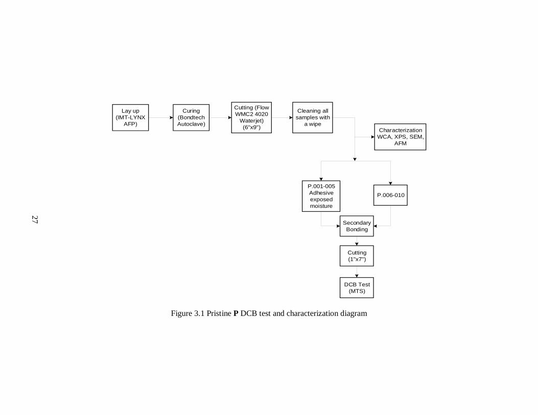
3.1 EXPERIMENTAL OVERVIEW
The purpose of this study is to determine the optimum APPJ treatment parameters
of CFRP surface preparation using the Open-air APPJ system by Plasmatreat®
(Steinhagen, Germany). The treatment conditions were used to determine how the bond
quality between an adhesive and composite material might be improved. For that
purpose, two main DCB test groups were selected: (1) pristine (non-treated) P detailed in
Figure 3.1, and (2) treated T detailed in Figure 3.2. The DCB test was applied to each test
coupon to calculate the opening Mode I interlaminar fracture toughness while
simultaneously observing the occurring failure mode. Characterization samples were
prepared to determine the surface characteristics prior to (pristine P) and after treatment
(treated T).
This chapter details all experimental procedures that were conducted in a
standardized fashion. The details include (1) materials, (2) the DCB test coupons
manufacturing, (3) the characterization samples, (4) each surface characterization method
for contact angle measurement, surface chemical modifications, and surface
morphological and topographical changes, and finally (5) the performed DCB test, and
the calculations of the 𝐺𝐼𝐶 and 𝐺𝐼𝑃, to determine the failure mode after DCB tests.
27
Cutting (Flow
WMC2 4020
Waterjet)
(6"x9")
Curing
(Bondtech
Autoclave)
Cleaning all
samples with
a wipe
Lay up
(IMT-LYNX
AFP)
P.006-010
P.001-005
Adhesive
exposed
moisture
DCB Test
(MTS)
Secondary
Bonding
Cutting
(1"x7")
Characterization
WCA, XPS, SEM,
AFM
Figure 3.1 Pristine P DCB test and characterization diagram

28
Treatment
T.S1V1D1 T.S1V2D1
DCB Test
(MTS)
Secondary
Bonding
Cutting
(1"x7")
T.S1V3D1 T.S2V1D1 T.S2V2D1
DCB Test
(MTS)
Secondary
Bonding
Cutting
(1"x7")
T.S2V3D1 T.S3V1D1 T.S3V2D1
DCB Test
(MTS)
Secondary
Bonding
Cutting
(1"x7")
T.S3V3D1T.S1V2D0
DCB Test
(MTS)
Secondary
Bonding
Cutting
(1"x7")
T.S3V2D0
DCB Test
(MTS)
Secondary
Bonding
Cutting
(1"x7")
Cleaning all
samples with
a wipe
Characterization
WCA, XPS, SEM,
AFM
Characterization
WCA, XPS, SEM,
AFM
Characterization
WCA, XPS, SEM,
AFM
Characterization
WCA, XPS, SEM,
AFM
Characterization
WCA, XPS, SEM,
AFM
Characterization
WCA, XPS, SEM,
AFM
Figure 3.2 Treated T DCB test and characterization diagram

29
3.2 MATERIAL AND TEST COUPON PREPARATION
3.2.1 Materials
In this research, Hexcel® IM7/8552 prepreg, which consists of an 8552 epoxy
resin and unidirectional intermediate modulus IM7 carbon fiber reinforcement, was used
to fabricate a 35” x 25” [0]9 composite panel in unidirectional configurations with a post
cure thickness of approximately 1.3 mm. Metlbond 1515-3M epoxy film adhesive, which
is commonly used in the aircraft industry due to its mechanical properties, is used to bond
the two laminates [108] creating an overall thickness of approximately 2.75 mm. J-B
Weld adhesive was used to bond aluminum hinges, needed for the DCB test, to the
adhesive bonded laminates.
A large roll of adhesive film was delivered in a moisture-proof bag with
desiccants. However, due to the current experimental process, only small adhesive strips
were used, leaving the rest of the adhesive to be exposed to moisture and atmosphere. To
avoid continuous exposure to the open air, the exposed Metlbond on the outer-most layer
of the roll was cut and discarded while the rest of the adhesive roll was heat sealed in a
bag with desiccants after removing as much air as possible. The adhesive roll was then
left under a fan for 5 hours at room temperature before determining that it had been
completely thawed. Once this process had been completed, the roll was removed from the
bag and individual 7” x 7” pieces were cut. Then, they were heat sealed in MIL-spec
bags, by use of a tabletop impulse heat sealer after removing air content from the bag,
and refrozen to protect the film from moisture and the surrounding atmosphere. This
process improved test preparation efficiency as only one small, sealed bag was used for
each bonded laminate that was tested.

30
3.2.2 Composite Production
Hexcel® IM7/8552 prepreg was laid up with 9-plies [0]9 by an IMT® LYNX
AFP machine shown in Figure 3.3. The AFP composite manufacturing flowchart is
shown in Figure A.1. Staggering of the 0° orientations were programmed in the toolpath
generation software. After the AFP laid up the composite on uncoated, nylon Wrightlon®
8400 Bagging Film, the panel was placed between two stainless steel compression plates
which had previously been sealed with Frekote B-15, to ensure there were no leaks
during a full vacuum due to scratches, and cured with a release agent Frekote 770-NC. A
vacuum bagging technique was applied with a full vacuum in 15-psig pressure. The
autoclave temperature was increased to 225 °F at a rate of 5 °F per/min. and held at this
temperature for 60 minutes. The vacuum was vented when the pressure reached 30 psig
as the pressure was increased to 100 psig, while the temperature was increased to 350 °F
at a rate of 5 °F/min. The temperature was held at 350 °F for 120 minutes and was then
cooled to 150 °F at a rate of 5 °F per/min. at the vented pressure according to the cure
cycle as shown in Figure 3.4 [109]. The autoclave cure cycle flowchart is shown in
Figure A.2.
Figure 3.3 AFP lay-up process

31
Figure 3.4 Cure cycle of Hexcel IM7/8552 [109]
Each manufactured composite panel was designed to accommodate 9 individual
6” x 9” laminates; these, along with the rest of the dimensions associated with the
composite panel, are shown in Figure 3.5.
Figure 3.5 Composite panel dimension
44
44
9
6
0.15
35
26
0 degree fiber direction

32
3.2.3 Groups of Composite Samples
The composite panel was cut into 9 laminates with a Flow® WMC2 Waterjet. In
addition, 10 mm x 10 mm samples were also cut for SEM, AFM, and XPS while 25 mm
x 50 mm samples were cut for WCA surface characteristic analysis. Then, we cut 10 mm
x 10 mm samples to allow them to fit into the sample chambers as it would not have been
possible to cut these pieces after plasma treatment without contamination. Two sets of
test groups, pristine (non-treated) P and treated T were investigated to determine the
effects of plasma treatment on a CFRP. These groups and their subgroups are labeled in
Table 3.1 while showing their test number description in Table 3.2, and the
characterization samples are shown in Table 3.3. These characterization samples differ
from the DCB test laminate groups in the sense that overlap was not used; instead, only
one pass of the plasma jet nozzle was applied to these samples.
Table 3.1 DCB test groups
Groups Test Number Laminate
Number 6” x 9”
Number
of Tests
Treatment
Speed (in/s)
Treatment
Overlap (%)
Pristine P P.001-005 2 5 - -
P.006-010 2 5 - -
Treated T
T.S1V1D1 2 5 0.1 25
T.S1V2D1 2 5 0.1 50
T.S1V3D1 2 5 0.1 75
T.S1V2D0 2 5 0.1 50
T.S2V1D1 2 5 0.5 25
T.S2V2D1 2 5 0.5 50
T.S2V3D1 2 5 0.5 75
T.S3V1D1 2 5 1.0 25
T.S3V2D1 2 5 1.0 50
T.S3V3D1 2 5 1.0 75
T.S3V2D0 2 5 1.0 50

33
Table 3.2 DCB test number description and plasma process parameters
P. Pristine -
T. Treated -
S1 Treatment speed 1 0.1 in/s
S2 Treatment speed 2 0.5 in/s
S3 Treatment speed 3 1.0 in/s
V1 Treatment overlap 1 25%
V2 Treatment overlap 2 50%
V3 Treatment overlap 3 75%
D0 Distance from the nozzle to the surface 0 0.25 in
D1 Distance from the nozzle to the surface 1 0.5 in
.001 Test number -
Table 3.3 Characterization samples
Method Groups Treatment
Speed (in/s)
Distance
(in)
Number of
Samples
Treatment
Overlap (%)
WCA
SEM
AFM
XPS
Pristine - Treated 0.10
0.5 1 1 pass with nozzle
Pristine - Treated 0.10 0.25 1 1 pass with nozzle
Pristine - Treated 0.50 0.5 1 1 pass with nozzle
Pristine - Treated 1.0 0.5 1 1 pass with nozzle
Pristine - Treated 1.0 0.25 1 1 pass with nozzle
Along with the different plasma parameters, the effect of moisture on adhesive
was also explored, providing two different pristine P tests numbered in Table 3.1. The
first DCB tests (P.001-005) had been bonded together with adhesive which had not been
sealed in a moisture-proof bag. That had been left wrapped in a plastic bag with its open
top folded over. It was closed off to moisture, but not sealed, whereas the second (P.006-
010) was bonded with an adhesive which had been sealed in moisture-proof bags.

34
3.2.4 DCB Test Coupon Assembly and Specifics
A non-adhesive FEP film by CS Hyde®, a Metlbond 1515-3M film adhesive, and
two of the composite laminates 6” x 9” were used to assemble each test coupon. The FEP
film was cut into a strip approximately 4.15” x 6” to be used as a site for the initial
delamination [39] meant to initiate the crack tip of the propagation along the DCB test
coupon [110]. This film had a thickness of 13 µm, which adheres to the ASTM D5528
suggestion of using an insert film with a thickness of no more than 13 μm [39].
The initial assembly of a test coupon consisted of the following details:
1. After taking out the adhesive from the freezer and letting it thaw until it
reached the room temperature, it was cut into 4.85” x 6” strip.
2. Before the assembly of the coupon, each laminate in the pristine P test
group was wiped with a Kimberly-Clark Kimtech W4 alcohol wipe, while
those in the treated T group were wiped before treatment.
3. During this secondary bonding process, FEP film was inserted at the end
of the laminate while the remaining part of the composite was covered by
the adhesive as shown in Figure 3.6.
Figure 3.6 Laminates bonding assembly
Insert Adhesive Composite laminates
0 orientation

35
The application of the adhesive strip consisted of removing the outside layer of
protection and rolling the paper-backed side of the strip onto one end of the laminate as
seen in Figure 3.7a & b. The FEP film was then placed in the remaining uncovered area
of the laminate. Both films were then completely covered with the second laminate and
rolled again on both outer sides of the composite shown in Figure 3.7c & d. The bonding
laminates flowchart is shown in Figure A.3.
(a) (b)
(c) (d)
Figure 3.7 Adhesive bonding application
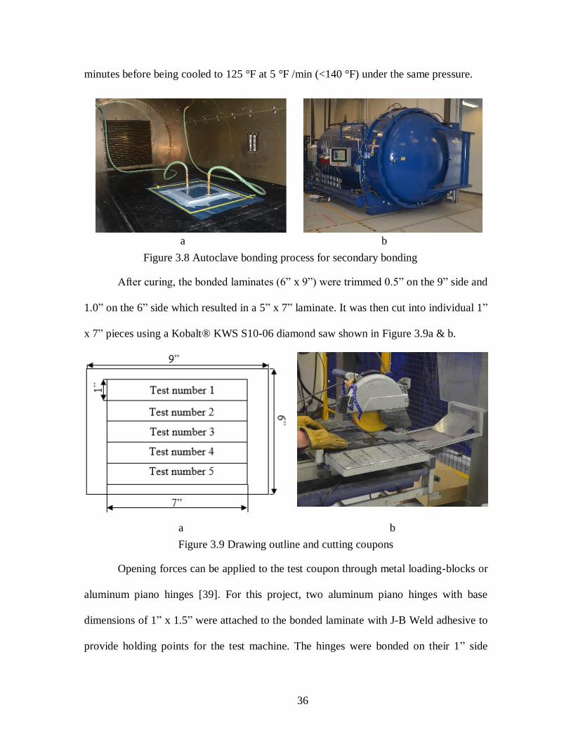
Vacuum bagging technique was used where the sandwiched laminates were
placed upon a nylon film between two steel plates, and vacuum sealed as seen in Figure
3.8a. An autoclave by Bondtech®, which is shown in Figure 3.8b, was used for the
recommended Metlbond 1515-3M curing cycle. We applied a 45 psi pressure, and the
temperature was increased to 350 °F from room temperature at a 5 °F /min
(recommended at a 1-5 °F/min). The temperature was held constant (350±10 °F) for 120
36
minutes before being cooled to 125 °F at 5 °F /min (<140 °F) under the same pressure.
a b
Figure 3.8 Autoclave bonding process for secondary bonding
After curing, the bonded laminates (6” x 9”) were trimmed 0.5” on the 9” side and
1.0” on the 6” side which resulted in a 5” x 7” laminate. It was then cut into individual 1”
x 7” pieces using a Kobalt® KWS S10-06 diamond saw shown in Figure 3.9a & b.
Opening forces can be applied to the test coupon through metal loading-blocks or
aluminum piano hinges [39]. For this project, two aluminum piano hinges with base
dimensions of 1” x 1.5” were attached to the bonded laminate with J-B Weld adhesive to
provide holding points for the test machine. The hinges were bonded on their 1” side
a
b
b
BN Figure 3.9 Drawing outline and cutting coupons

37
along the 1” end of the specimen containing the FEP film shown in Figure 3.10. Before
bonding each hinge to the specimen, the hinge surface was abraded with 120 grit
sandpaper prior to being cleaned with acetone and alcohol respectively. Meanwhile, the
surface of the composite was also cleaned in that order as well. After applying the
adhesive to the 1” side of both piano hinges, one clamp was used to hold the hinges to the
specimen’s surface while the cure took place. The adhesives’ curing time, according to
the J-B weld technical document, is 15-24 hours at room temperature and the coupons
were cured for approximately 24 hours. The hinge bonding flowchart is shown in Figure
A.4.
Figure 3.10 Clamping piano hinge while J-B Weld cures
The resulting DCB test coupon, which is shown in Figure 3.11, had a uniform
thickness and width with the final dimensions of the DCB test coupon given in Table 3.4.
Table 3.4 DCB test coupon dimensions
Length L
(in)
Width b
(in)
Thickness h
(in)
Initial Crack Length a0
(in)
7 1
(25.4)
~0.108 (~2.75 mm) ~2 (50 mm)

38
Figure 3.11 DCB test coupon assembly
3.3 OPEN-AIR PLASMA TREATMENT
Open-air plasma technology by Plasmatreat® was used for the treatment of the
laminate surfaces in the treated T test group. It is described as an atmospheric pressure
plasma jet (APPJ) [19], and plasma is generated in an arc and extended with the gas flow
[35]. It creates an electrical discharge inside the jet and blows it out as a stream of air,
which is known as open air plasma. This plasma treatment can be considered indirect
contact since the plasma is created within the jet; however, the plasma discharge range
could be extended 1-2 cm past the end of the jet nozzle [35]. The plasma is generated and
dispensed from the nozzle as a result of the high voltage between the stator and the rotor.
It supplies a chemical-free micro-fine cleaning and activates surfaces before bonding.
The FG5002S plasma generator in Figure 3.12 and RD1004 plasma rotary nozzle in
Figure 3.13 were used for the process and dry compressed air was used as the gas. A PTF
2647-2 stainless steel nozzle with an angle of 14° was used to create a treatment width of
approximately 1”.
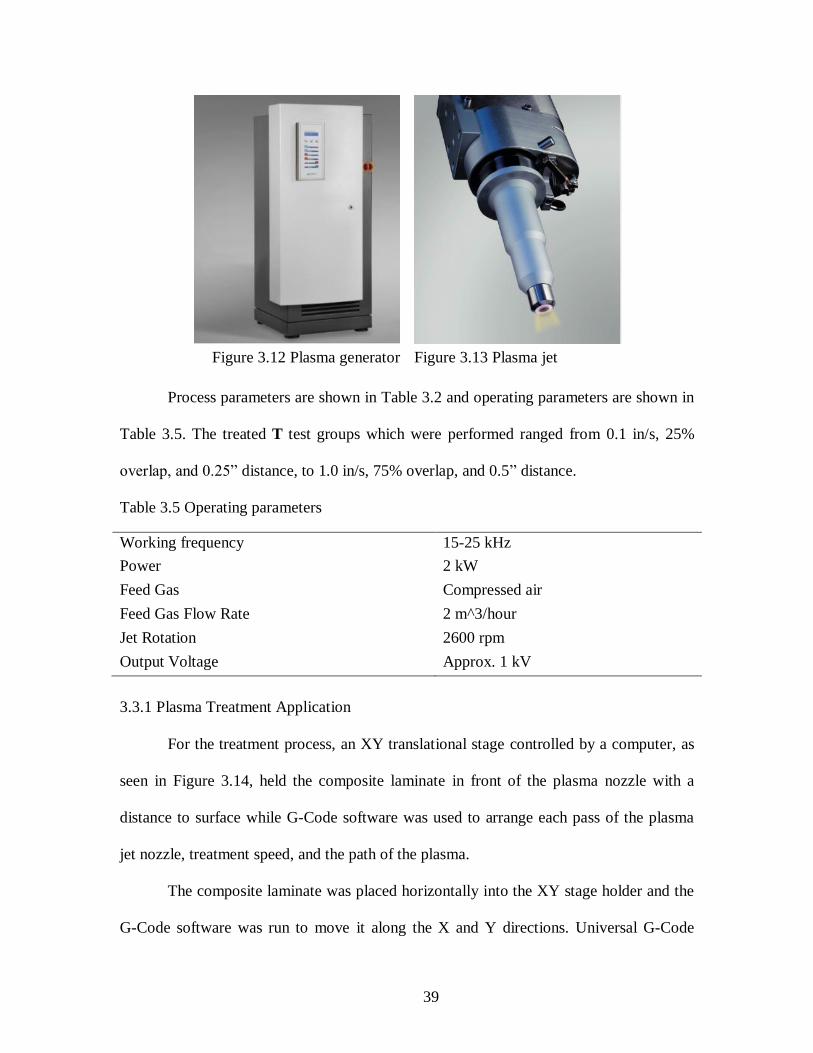
39
Figure 3.12 Plasma generator Figure 3.13 Plasma jet
Process parameters are shown in Table 3.2 and operating parameters are shown in
Table 3.5. The treated T test groups which were performed ranged from 0.1 in/s, 25%
overlap, and 0.25” distance, to 1.0 in/s, 75% overlap, and 0.5” distance.
Table 3.5 Operating parameters
Working frequency 15-25 kHz
Power 2 kW
Feed Gas Compressed air
Feed Gas Flow Rate 2 m^3/hour
Jet Rotation 2600 rpm
Output Voltage Approx. 1 kV
3.3.1 Plasma Treatment Application
For the treatment process, an XY translational stage controlled by a computer, as
seen in Figure 3.14, held the composite laminate in front of the plasma nozzle with a
distance to surface while G-Code software was used to arrange each pass of the plasma
jet nozzle, treatment speed, and the path of the plasma.
The composite laminate was placed horizontally into the XY stage holder and the
G-Code software was run to move it along the X and Y directions. Universal G-Code

40
Sender allowed for the visualization of the path of the code and control of the hardware
itself, while also allowing the upload of G-Code files and alteration of stepper motor
settings. The plasma treatment flowchart is shown in Figure A.5.
Figure 3.14 Plasma treatment system
Prior to the plasma treatment application, each laminate in the treated T group
was wiped with a Kimberly-Clark® Kimtech P2 Aviation Wipe. Each plasma jet nozzle
was placed at a distance of 0.5” or 0.25” from the surface of the composite part, based on
the experimental selection.
Treatment overlap was not used for characterization samples because the samples’
dimensions were too small to use the overlap. A single pass of the plasma jet nozzle was
sufficient. One sample was used for every set of test parameters (treatment speed;
distance from the plasma nozzle to the composite surface); this also included pristine
samples (wiped).
After plasma treatment, all samples were wrapped in aluminum foil to prevent the
contamination of their surfaces by air pollutants until subsequent bonding or
characterization. All laminates were bonded with Metlbond for the test coupon or

41
analyzed with WCA, XPS, SEM, and AFM methods within 1 hour of the treatment, and
they were kept in aluminum foil until they were ready to be measured.
3.4 SURFACE CHARACTERIZATION
3.4.1 Water Contact Angle (WCA)
The WCA was measured using a SA3001 Surface Analyst device by BTG Labs®
(Cincinnati, OH), shown in Figure 3.15, and the contact angle flowchart is shown in
Figure A.6. The device measures the receding contact angle with a pulsed stream of
nanoliter-sized microdroplets [49], a method which is commonly known as the ballistic
deposition method. Both the volume and the diameter of the drop are used to calculate the
approximate contact angle by averaging established geometric standards for similarly
sized droplets [88]. The contact angle, which is calculated this way, is more inclusive and
provides a more accurate representation of the surface energy in the area surrounding the
drop [52].
Figure 3.15 Surface analyst device
When a drop detection was not defined well as shown in Figure 3.16, it was
rejected; however, when the drop detection was well defined shown in Figure 3.17, it was
an acceptable measurement of the contact angle.
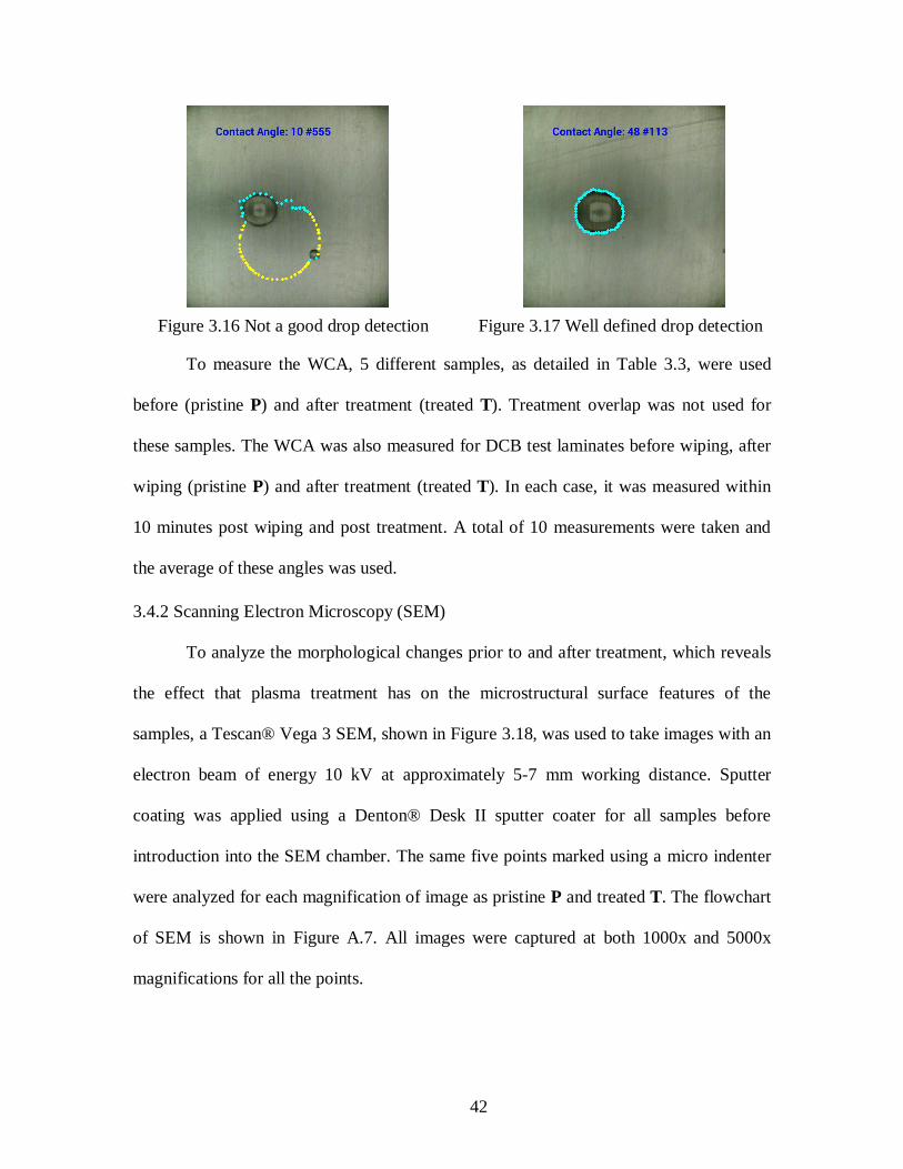
42
Figure 3.16 Not a good drop detection Figure 3.17 Well defined drop detection
To measure the WCA, 5 different samples, as detailed in Table 3.3, were used
before (pristine P) and after treatment (treated T). Treatment overlap was not used for
these samples. The WCA was also measured for DCB test laminates before wiping, after
wiping (pristine P) and after treatment (treated T). In each case, it was measured within
10 minutes post wiping and post treatment. A total of 10 measurements were taken and
the average of these angles was used.
3.4.2 Scanning Electron Microscopy (SEM)
To analyze the morphological changes prior to and after treatment, which reveals
the effect that plasma treatment has on the microstructural surface features of the
samples, a Tescan® Vega 3 SEM, shown in Figure 3.18, was used to take images with an
electron beam of energy 10 kV at approximately 5-7 mm working distance. Sputter
coating was applied using a Denton® Desk II sputter coater for all samples before
introduction into the SEM chamber. The same five points marked using a micro indenter
were analyzed for each magnification of image as pristine P and treated T. The flowchart
of SEM is shown in Figure A.7. All images were captured at both 1000x and 5000x
magnifications for all the points.

43
Figure 3.18 Tescan Vega SBU variable pressure SEM
5 samples were used for SEM analysis in Table 3.3. Treatment overlap was not
used, and in each case, SEM was performed within 1 hour of either wiping (pristine P) or
after treatment (treated T).
3.4.3 Atomic Force Microscopy
The surface topography was also studied with AFM at room temperature and
under ambient conditions using a Nanoscope® Dimension 3100 Controller. Scanning
was achieved in a 5 µm x 5 µm area in the non-contact mode with a standard silicon tip.
The root mean square (rms) roughness and three-dimensional (3D) images were obtained
by using the Nanoscope software.
3.4.4 X-ray Photoelectron Spectroscopy (XPS)
Kratos® Axis Ultra XPS, shown in Figure 3.19, was used to link surface free
energy evolution to the surface elemental composition and chemical bonds before and
after treatment. A beam of X-rays simultaneously measures the kinetic energy and
number of the electrons that escape from the surface of the test material. It analyzed the
atomic composition of the top 10nm of the composite surface, specifically used for the
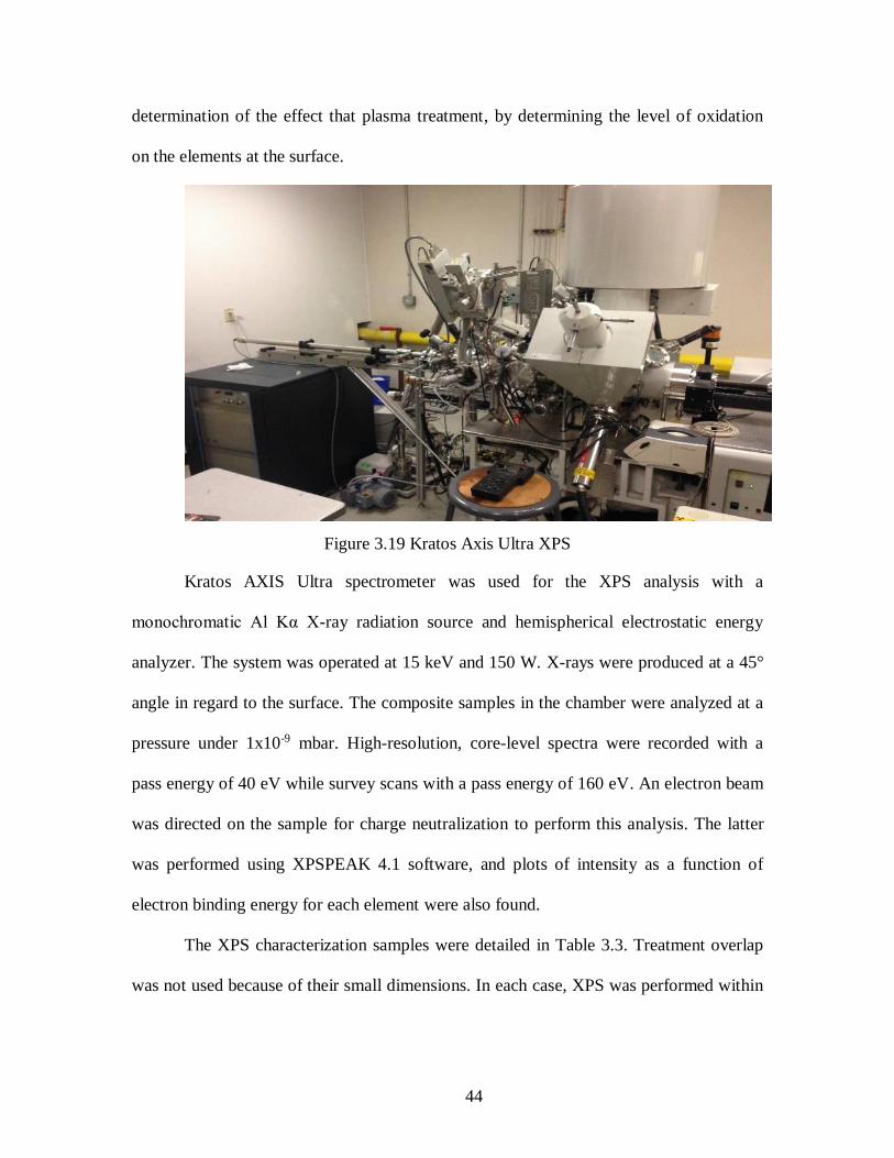
44
determination of the effect that plasma treatment, by determining the level of oxidation
on the elements at the surface.
Figure 3.19 Kratos Axis Ultra XPS
Kratos AXIS Ultra spectrometer was used for the XPS analysis with a
monochromatic Al Kα X-ray radiation source and hemispherical electrostatic energy
analyzer. The system was operated at 15 keV and 150 W. X-rays were produced at a 45°
angle in regard to the surface. The composite samples in the chamber were analyzed at a
pressure under 1x10⁻⁹ mbar. High-resolution, core-level spectra were recorded with a
pass energy of 40 eV while survey scans with a pass energy of 160 eV. An electron beam
was directed on the sample for charge neutralization to perform this analysis. The latter
was performed using XPSPEAK 4.1 software, and plots of intensity as a function of
electron binding energy for each element were also found.
The XPS characterization samples were detailed in Table 3.3. Treatment overlap
was not used because of their small dimensions. In each case, XPS was performed within

45
1 hour after wiping or after treatment. The same area was analyzed each time to measure
the surface chemical composition.
3.5 DOUBLE CANTILEVER BEAM (DCB) TEST
The DCB test, which its schematic is shown in Figure 3.20, was performed on the
adhesively bonded composite coupons with a MTS® testing machine (MTS,
Minneapolis, MN) which is shown in Figure 3.21. It is an experimental test method
designed to determine the opening Mode I interlaminar fracture toughness of
unidirectional CFRP using the DCB test coupon in Figure 3.11, and the calculation is
based on its width, crack-propagation length, the applied load and displacement of the
DCB test coupon. This test aims to study the optimal plasma process parameters. The
DCB test flowchart is shown in Figure A.8.
Figure 3.20 DCB test schematic
The load was applied to the end of the test coupon while the other end was free, as
seen in Figure 3.21. The resistance to crack initiation and propagation was to be

46
determined under the crack-opening mode, Mode 1. The Mode 1 pre-crack was used to
create an initial site of delamination on the coupon.
Figure 3.21 DCB test setup
A load and displacement curve was recorded with MTS® TestSuiteTM TW Elite
software during the test. Two cameras were set up with the Open Broadcast Software to
concurrently record the actions of the DCB test coupon, as seen in Figure 3.21, and the
load and crosshead displacement values displayed on the software running on the
computer screen. This allowed for the tracking of the propagation of the crack at different
load and displacement values by viewing the marks on the side of the test coupon. The
initiation and propagation values of GIC and GIP were calculated using this recorded data
with the Modified Beam Theory (MBT) method.
The first 5 mm past initial crack (delamination) was marked every 1 mm, the
following 45 mm was marked every 5 mm, prior to marking the 46th through 50th mm

47
every 1 mm, as shown in Figure 3.22. The remaining length of the coupon was marked
every 5 mm to provide a reference of delamination crack during the test.
Figure 3.22 DCB test coupon marked
The total crack propagation from the initial crack tip was approximately 50 mm
for DCB tests. Three different loading and unloading methods were used in accordance
with ASTM D5528-01 [39]. The first loading sequence was used to pre-crack the test
coupon about 3-5 mm following the length of the insert. That was done to eliminate the
initial spike in the results which could result in outliers in the data. The second loading
sequence propagated the crack an additional 50 mm [110]; this second sequence was used
as the main group of data points. The third loading sequence was initiated to conclude
which failure mode existed.
3.5.1 Initial Loading
The piano hinges were attached to the MTS test machine in Figure 3.21 where the
DCB test was performed. The ASTM D5528-01 [39] gives the loading rate for the DCB
test coupon with 1-5 mm/min; however, the coupon was loaded at a constant crosshead
rate of 1.0 in/min. A point on the load-displacement curve was made, marking the

48
beginning of the crack movement from the insert, which was observed from the recording
of the edge of the coupon.
Loading was stopped as soon as the delamination crack growth was seen to reach
an increment of 3 to 5 mm. At this point, the coupon was unloaded at a constant cross-
head rate of up to 1.0 in/min. The position of the tip of the pre-crack was marked on both
sides of the coupon; if these marks differed by more than 2 mm it was noted in the report,
as this variation could indicate asymmetrical loading [39].
3.5.2 Reloading
The load was reapplied on the coupon, at the same crosshead rate of 1.0 in/min
and a point on the load-displacement curve was made, marking the crack movement from
the tip of the pre-crack on the edge of the coupon. The load and displacement data were
recorded at every 5 mm increment until the delamination crack had propagated at least 45
mm from the tip of the pre-crack, and at every 1 mm increment of crack growth for the
following and final 5 mm of delamination propagation. When delamination crack reached
50 mm, loading was stopped and it was unloaded at a constant crosshead rate of up to 1.0
in/min.
To determine which failure mode occurred on the bonded area, the test coupon
was reloaded again at the same crosshead rate of 1.0 in/min until the end of the coupon
without stopping.
3.5.3 Modified Beam Theory (MBT) Method
The modified beam theory equation was used to calculate the interlaminar
fracture toughness (𝐺𝐼𝐶) in equation (2.8) using the load and crosshead distance data
recorded during the test.

49
The (𝐺𝐼𝑃) value given in equation (3.1) was calculated by taking the area under
the load and displacement curve (E) and dividing it by the propagation length (a)
multiplied by the width of the coupon (b). This number represents a more general value
to classify fracture toughness.
𝐺𝐼𝑃 =𝐸
𝑎𝑥𝑏
(3.1)
3.5.4 Delamination Resistance Curve (R Curve)
Resulting from a DCB test, delamination grows from the tip of the insert and a
resistance-type fracture behavior develops in the adhesive where the calculated 𝐺𝐼𝐶 first
increases monotonically [39]. A resistance R curve shown in Figure 3.23 shows the
relationship between the strain energy release rate (𝐺𝐼𝐶) and the delamination length
(crack length, a).
Figure 3.23 Delamination resistance curve (R curve) [39]
3.5.5 Failure Modes
Fracture surfaces were analyzed visually to decide what mode of failure the test
resulted in. According to ASTM D5573 [106], seven failure modes were adapted as
shown in Figure 3.24. They each have the ability to occur on the test coupon [106].

50
(a) (b)
(c) (d)
(e) (f)
(g) (h)
Figure 3.24 DCB failure modes a) Adhesive failure b) Cohesive failure c) Thin layer
cohesive failure d) Adhesion promoter to substrate e) Adhesive to adhesion promoter
f) Fiber tear failure g) Light fiber tear failure h) Stock break failure
Adhesion
Promoter
Adhesive
Substrate

51
RESULTS AND DISCUSSION
This chapter presents the experimental results of the conducted test plan to
identify the effect of APPJ treatment. It discusses both (1) the characterization methods:
WCA, SEM, AFM, and XPS; and (2) the DCB tests: Mode I interlaminar fracture
toughness and failure mode. Characterization samples were plasma treated following the
same sequence for all the test specimens. The first three samples were treated with speeds
of 0.1 in/s (S1), 0.5 in/s (S2) and 1.0 in/s (S3) at 0.5 in (D1) distance from the plasma jet
nozzle to the surface respectively, while samples 4 and 5 were treated with a treatment
speed of 0.1 in/s (S1) and 1.0 in/s (S3) at distance of 0.25 in (D0) respectively. Treatment
overlap was not relevant for the characterization samples: they were treated with a single
pass of the plasma jet.
4.1 WATER CONTACT ANGLE (WCA)
The WCA results of the pristine P (in red) and treated T samples (in grey) are
shown in Figure 4.1. Results show that the amount of wiping did have an effect on the
contact angle; however, it varied due to the fact that it was done manually and thus it is
prone to human err. A sharp decrease in the contact angle was observed after treatment
for all the samples. The lowest angle (13.5°) was taken at conditions: D1 for distance, S1
for treatment speed. These conditions had the longest treatment duration which promoted
the low WCA. When the treatment speed increased at distance D1, we observed that the

52
contact angle also increased. The decrease in the contact angle demonstrates an
enhancing surface roughness [11], the formation of polar groups [11, 20] on the surface
through the increase of hydrophilicity when the treatment time was raised with a constant
distance [22]. Li et al [22], states that maximizing polar surface with a longer treatment
time causes the increase of surface wettability [11].
When distance decreased to 0.25 in (D0), an increase of the contact angle
occurred within the same treatment speeds. As such, we observed that the angle of
sample 4 was lower with treatment speed S1 than the contact angle of sample 5 with
speed S3. Results clearly indicate that surface hydrophilicity raised with lower contact
angle and the higher polar surface which has enhanced polar groups and oxidation after
treatment [26].
Figure 4.1 WCA for pristine and treated samples

53
In addition to the above five samples, WCA was also measured for each DCB test
laminate (6” x 9”), and the results are presented in: Figure 4.2 for Speed 1, Figure 4.3 for
Speed 2, Figure 4.4 for Speed 3, and Figure 4.5 for a refined selection. The contact angles
were within the range of 82°-89° for each laminate before wiping and showed a decrease
to a range of 55°-75° following the wiping process. However, it sharply dropped to the
10.9°-23.9° range following the surface plasma treatment. The lowest angle was
measured on the laminate treated with speed S2, overlap V1, and distance D1 in Figure
4.3 while the highest was recorded for the slowest treatment speed S1 with the highest
overlap V3, at the same distance D1, in Figure 4.2.
When the distance dropped to 0.25 in (D0) from plasma jet to composite surface,
the contact angle increased with the same treatment speed and overlap value.
Figure 4.2 WCA for pristine and treated samples (S1,V1-2-3, and D1)

54
Figure 4.3 WCA for pristine and treated samples (S2,V1-2-3, and D1)
Figure 4.4 WCA for pristine and treated samples (S3,V1-2-3, and D1)
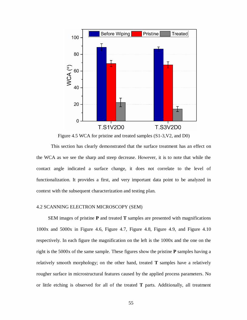
55
Figure 4.5 WCA for pristine and treated samples (S1-3,V2, and D0)
This section has clearly demonstrated that the surface treatment has an effect on
the WCA as we see the sharp and steep decrease. However, it is to note that while the
contact angle indicated a surface change, it does not correlate to the level of
functionalization. It provides a first, and very important data point to be analyzed in
context with the subsequent characterization and testing plan.
4.2 SCANNING ELECTRON MICROSCOPY (SEM)
SEM images of pristine P and treated T samples are presented with magnifications
1000x and 5000x in Figure 4.6, Figure 4.7, Figure 4.8, Figure 4.9, and Figure 4.10
respectively. In each figure the magnification on the left is the 1000x and the one on the
right is the 5000x of the same sample. These figures show the pristine P samples having a
relatively smooth morphology; on the other hand, treated T samples have a relatively
rougher surface in microstructural features caused by the applied process parameters. No
or little etching is observed for all of the treated T parts. Additionally, all treatment

56
speeds of APPJ with both distances D0 and D1 were able to remove all the impurities on
the surface, which helps to improve the bond itself [111].
(a) (b)
(c) (d)
Figure 4.6 Sample 1 SEM images a) Pristine M:1000x b) Pristine M:5000x
c) Treated M:1000x (S1, D1) d) Treated M:5000x (S1, D1)
(a) (b)
(c) (d)
Figure 4.7 Sample 2 SEM images a) Pristine M:1000x b) Pristine M:5000x
c) Treated M:1000x (S2, D1) d) Treated M:5000x (S2, D1)
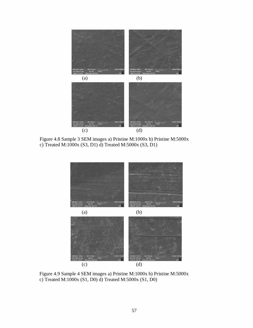
57
(a) (b)
(c) (d)
Figure 4.8 Sample 3 SEM images a) Pristine M:1000x b) Pristine M:5000x
c) Treated M:1000x (S3, D1) d) Treated M:5000x (S3, D1)
(a) (b)
(c) (d)
Figure 4.9 Sample 4 SEM images a) Pristine M:1000x b) Pristine M:5000x
c) Treated M:1000x (S1, D0) d) Treated M:5000x (S1, D0)
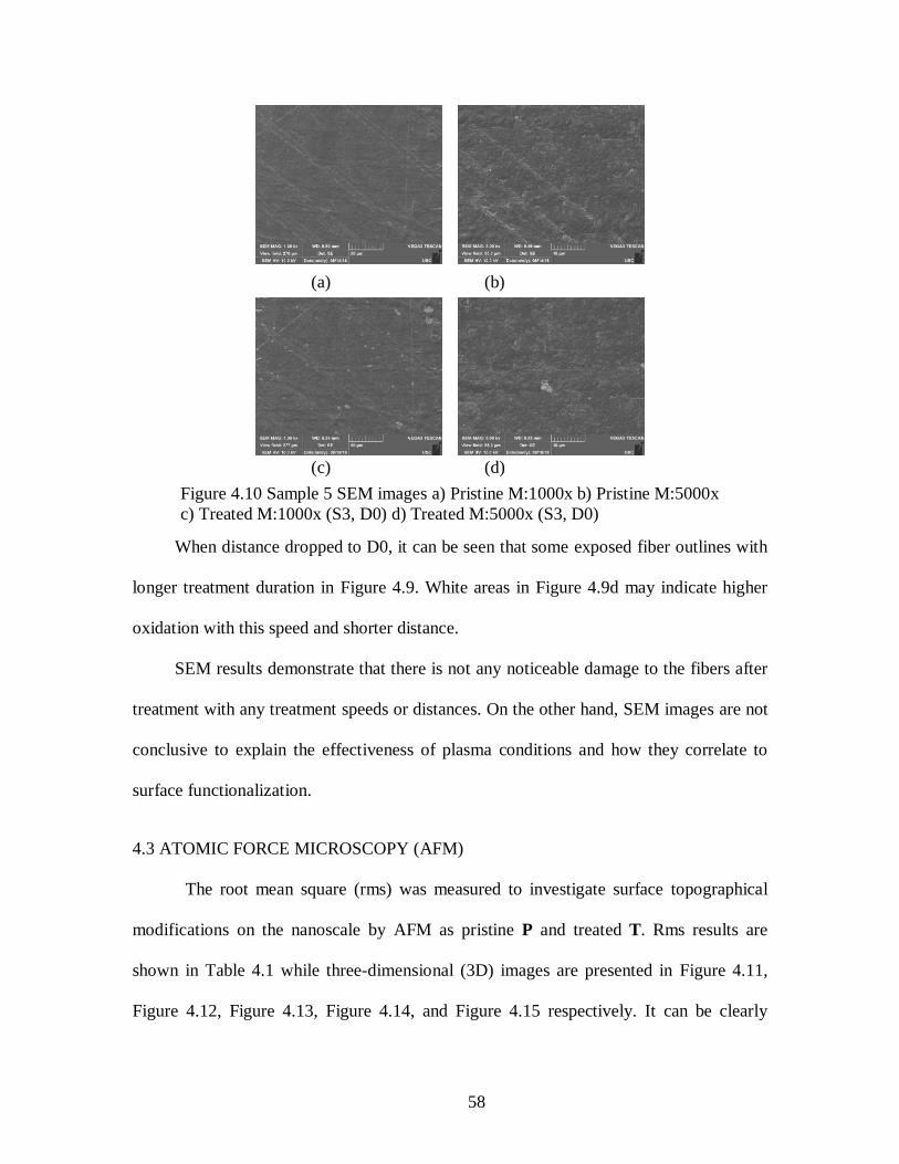
58
(a) (b)
(c) (d)
Figure 4.10 Sample 5 SEM images a) Pristine M:1000x b) Pristine M:5000x
c) Treated M:1000x (S3, D0) d) Treated M:5000x (S3, D0)
When distance dropped to D0, it can be seen that some exposed fiber outlines with
longer treatment duration in Figure 4.9. White areas in Figure 4.9d may indicate higher
oxidation with this speed and shorter distance.
SEM results demonstrate that there is not any noticeable damage to the fibers after
treatment with any treatment speeds or distances. On the other hand, SEM images are not
conclusive to explain the effectiveness of plasma conditions and how they correlate to
surface functionalization.
4.3 ATOMIC FORCE MICROSCOPY (AFM)
The root mean square (rms) was measured to investigate surface topographical
modifications on the nanoscale by AFM as pristine P and treated T. Rms results are
shown in Table 4.1 while three-dimensional (3D) images are presented in Figure 4.11,
Figure 4.12, Figure 4.13, Figure 4.14, and Figure 4.15 respectively. It can be clearly

59
observed and deduced that the surface roughness is increased for all the samples
following treatment. Figure 4.14b with treatment conditions: speed S1 and distance D0,
drastically differs with the steadier rougher surface from other images. Higher surface
roughness may increase adhesion [62]; however, one cannot correlate between treatment
speed and surface roughness according to the results.
Table 4.1 Rms surface roughness for pristine and treated samples
Treatment speed
(in/s)
Distance
(in)
Rms surface roughness
(nm)
Sample1 Pristine - - 12.576
Treated 0.1 0.5 29.937
Sample2 Pristine - - 10.965
Treated 0.5 0.5 37.370
Sample3 Pristine - - 22.300
Treated 1.0 0.5 42.360
Sample4 Pristine - - 25.307
Treated 0.1 0.25 35.170
Sample5 Pristine - - 16.954
Treated 1.0 0.25 23.647
a b
Figure 4.11 Sample 1 3D images a) Pristine b) Treated (S1, D1)
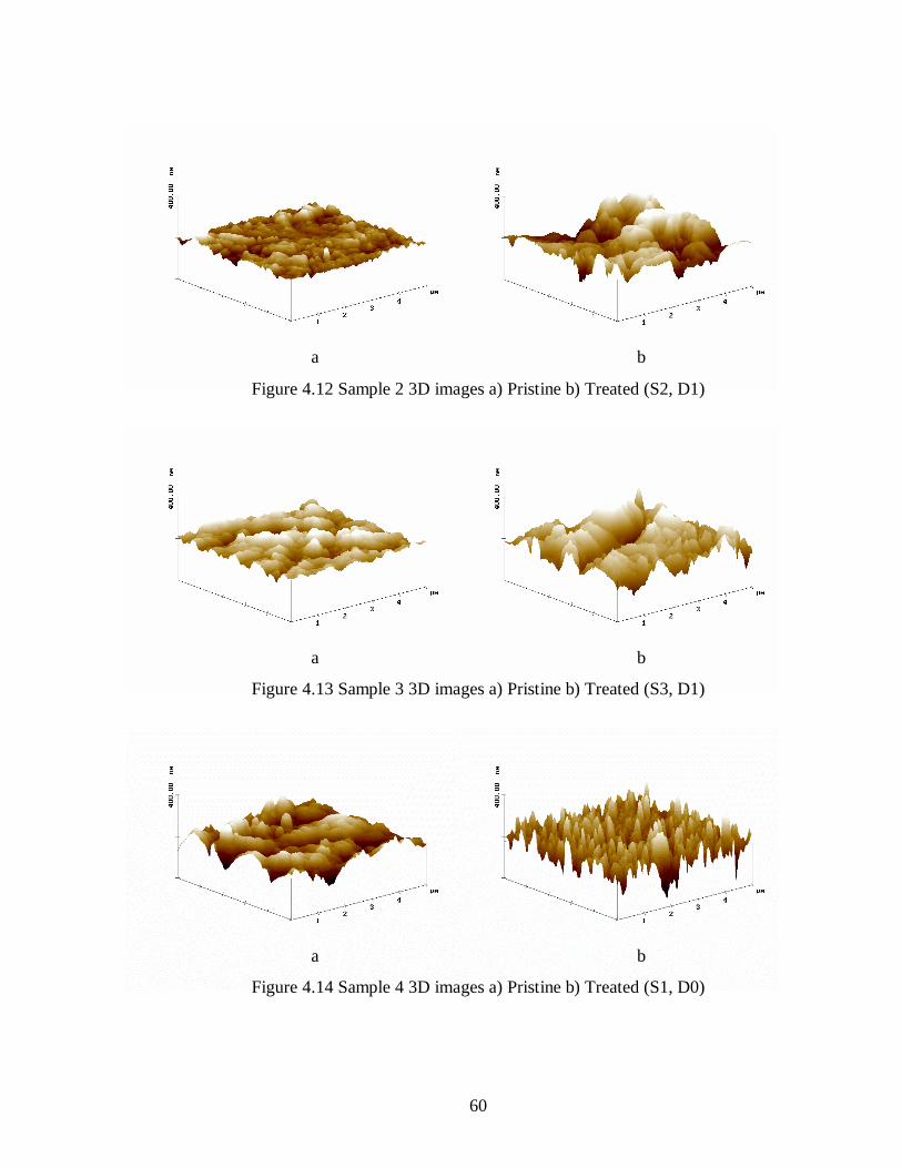
60
a b
Figure 4.12 Sample 2 3D images a) Pristine b) Treated (S2, D1)
a b
Figure 4.13 Sample 3 3D images a) Pristine b) Treated (S3, D1)
a b
Figure 4.14 Sample 4 3D images a) Pristine b) Treated (S1, D0)

61
a b
Figure 4.15 Sample 5 3D images a) Pristine b) Treated (S3, D0)
4.4 X-RAY PHOTOELECTRON SPECTROSCOPY (XPS)
XPS regional analysis was carried out on the pristine P and treated T samples to
investigate the observed quantitative atomic composition and functional group
differences through interactions between the composite surface and the APPJ treatment.
XPS atomic concentration with the ratios of O/C (in %) for the pristine P and
treated T samples are compared in Table 4.2. All the five surfaces were composed of
carbon (C1s), oxygen (O1s), nitrogen (N1s), sulfur (S2p) and silicon (Si2p). Silicon was
probably related to the contamination of stainless steel, by a mold release agent (Frekote
710-NC). The mold release agent consists of silicon compounds, and it was used during
the autoclave-curing process of the panel manufacturing.
XPS survey spectra analysis demonstrates C1s had the highest intensity prior to
and after treatment. The air APPJ treatment caused a significant reduction of carbon
concentration [20, 30, 112] and a slight increase of nitrogen for the last two samples, but
also a slight decrease of nitrogen for the first three samples. However, O1s intensity had a
remarkable increase [20, 30, 112, 113] after treatment due to the air in the plasma [22],
the reaction of free radicals and the unstable species interaction with oxygen from the

62
active species resides in the plasma. XPS results show sample 4 had a highest oxygen
content (hydrophilic behavior [7]) after treatment. It comes directly from the plasmas
interaction with the composite surface by enhancing oxygen-containing functional (polar)
groups [9, 20, 30], and decreasing carbon-containing groups. In other words, hydrophilic
chemical compositions increased while hydrophobic composition decreased [22]. The
surface oxygen-content enhancement correlates with better adhesive strength with epoxy
matrix [114], surface oxidation [21, 32] and improved wettability properties with surface
activation [11, 20]. Sulfur content showed a slight increase for sample 1, 4 and 5;
however, it decreased in small amounts for samples 2 and 3. The atomic silicon amount
showed a relatable behavior with a small increase for the samples 2, 3 and 5 while it
decreased for samples 1 and 4.
Table 4.2 XPS elemental composition of pristine and treated samples
Chemical composition
(%)
Atomic
ratio (%)
C O N S Si O/C
Pristine1 62.8 24.1 7.02 1.9 3.9 38
T.S1.D1 52.7 32.7 6.03 3.7 3.7 62
Pristine2 67.6 20.6 7.1 1.7 2.9 30
T.S2.D1 57.7 31.1 5.2 1.2 3 54
Pristine3 67.4 21 6.74 1.5 2.9 31
T.S3.D1 58.2 31.7 4.8 1 3.5 54
Pristine4 72.17 18.25 4.58 1.60 3.39 25
T.S1.D0 42.11 36.68 10.20 6.60 2.56 87
Pristine5 76.50 15.24 4.89 1.19 2.15 20
T.S3.D0 57.91 30.33 6.99 2.47 2.39 52

63
It is found that the O/C ratio, which represents functionalization levels [20],
increased significantly by showing the oxygen-containing groups which were introduced
to the surfaces of all the treated T samples [32]. O/C ratio of sample 4, which was treated
with the speed of S1 and distance D0, was highest due to more oxygenated surface with
longer treatment duration and closer distance.
The differences in bond structures, indicated from the XPS peak analysis, are
detailed in Table 4.3 for carbon and in Table 4.4 for oxygen and silicon. The
deconvolution analysis of carbon (C1s), oxygen (O1s), and silicon (Si2p) performed with
XPS peak 4.1 software is given as pristine P and treated T for sample 1 in Figure 4.16,
Figure 4.17, and Figure 4.18 respectively. The three peaks of C1s binding energies at
284.6 eV, 285.9±0.2 eV, and 288.5±0.2 eV correspond to C=C, C-N/C-C/C-O and O-
C=O components, respectively. (1) C=C double bond remained almost unchanged with a
0.2% increase for sample 1 while it decreased for other samples. (2) The C-N/C-C/C-O
group had decreased for sample 1; however, it was almost same for samples 2 and 3, and
it increased for samples 4 and 5 that with distance D0. (3) The O-C=O (ester or
carboxylic acid) functional group increased significantly for sample 1 compared to other
samples. Sample 4 showed a different behavior with speed S1 and distance D0 than other
samples creating C-O single bond at binding energy 289.6±0.2 [115].
The two peaks of O1s binding energies at 532±0.2 eV and 533.3±0.2 eV
correspond to C-O and C=O components, respectively. The C-O single bond was
detected with a small increase for sample 1, while decreased for other samples.
Therefore, the C=O group showed a similar behavior with the plasma treatment.

64
Figure 4.16 Sample 1 Carbon (C1s) deconvolution of pristine and treated
Figure 4.17 Sample 1 Oxygen (O1s) deconvolution of pristine and treated
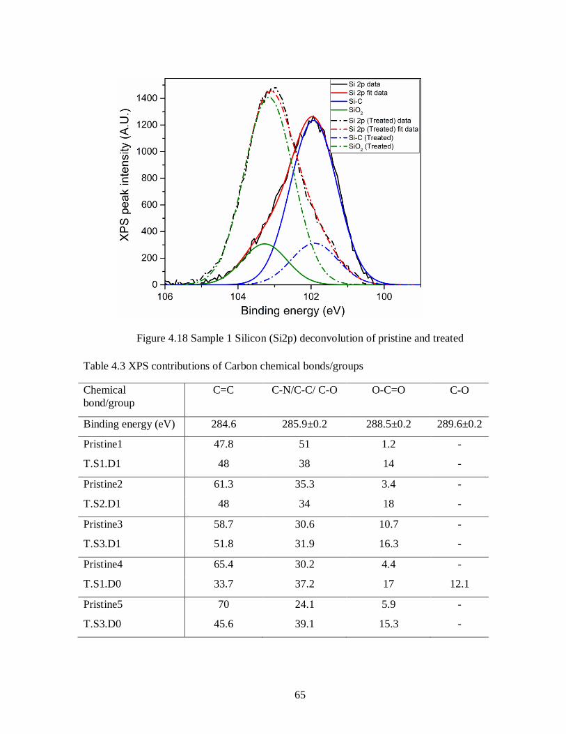
65
Figure 4.18 Sample 1 Silicon (Si2p) deconvolution of pristine and treated
Table 4.3 XPS contributions of Carbon chemical bonds/groups
Chemical
bond/group
C=C C-N/C-C/ C-O O-C=O C-O
Binding energy (eV) 284.6 285.9±0.2 288.5±0.2 289.6±0.2
Pristine1 47.8 51 1.2 -
T.S1.D1 48 38 14 -
Pristine2 61.3 35.3 3.4 -
T.S2.D1 48 34 18 -
Pristine3 58.7 30.6 10.7 -
T.S3.D1 51.8 31.9 16.3 -
Pristine4 65.4 30.2 4.4 -
T.S1.D0 33.7 37.2 17 12.1
Pristine5 70 24.1 5.9 -
T.S3.D0 45.6 39.1 15.3 -

66
Prior to treatment, the silicon present on the samples was predominantly SiC;
however, the SiO2 amount increased significantly for all the treated T samples, showing
the oxidation of silicon, while SiC observed a sharp decrease [116, 117]. SiC XPS peak
was not found for sample 4 after treatment. Instead, SiO2 was detected at binding
energies 103.3±0.2 eV and 105 eV showed all silicon oxidized [118, 119].
Table 4.4 XPS contributions of Oxygen and Silicon chemical bonds/groups
O 1s Si 2p
Chemical bond/group C-O C=O SiO2 SiC
Binding energy (eV) 532±0.2 533.3±0.2 103.3±0.2 105 101.8±0.1
Pristine1 70 30 20 80
T.S1.D1 72 28 82 18
Pristine2 78.6 21.4 15.7 84.3
T.S2.D1 74 26 81 19
Pristine3 79.6 20.4 15 85
T.S3.D1 73 27 68 32
Pristine4 80.9 19.1 27 73
T.S1.D0 76.5 23.5 66.2 33.8 -
Pristine5 79.6 20.4 30.7 69.3
T.S3.D0 60 40 75.4 24.6
This section clearly validated that plasma treatment decreased carbon content,
increased oxygen content, oxygen functional group, and O/C ratio. Functionalization
level (O/C) of sample 4 was the highest with a ratio of 87%. That can be probably
attributed to the prolonged treatment time which caused activated sites at the initiation of
the treatment cycle to become reactive with atmospheric radicals. Therefore, silicon
experienced oxidation and sample 4 with S1 and D0 showed a 100% oxidize appearing
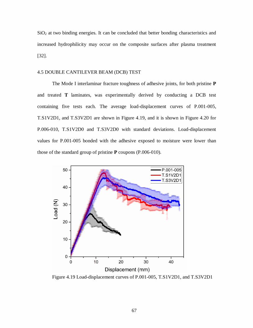
67
SiO2 at two binding energies. It can be concluded that better bonding characteristics and
increased hydrophilicity may occur on the composite surfaces after plasma treatment
[32].
4.5 DOUBLE CANTILEVER BEAM (DCB) TEST
The Mode I interlaminar fracture toughness of adhesive joints, for both pristine P
and treated T laminates, was experimentally derived by conducting a DCB test
containing five tests each. The average load-displacement curves of P.001-005,
T.S1V2D1, and T.S3V2D1 are shown in Figure 4.19, and it is shown in Figure 4.20 for
P.006-010, T.S1V2D0 and T.S3V2D0 with standard deviations. Load-displacement
values for P.001-005 bonded with the adhesive exposed to moisture were lower than
those of the standard group of pristine P coupons (P.006-010).
Figure 4.19 Load-displacement curves of P.001-005, T.S1V2D1, and T.S3V2D1

68
In comparison, the DCB test results showed that coupons made from laminates
with APPJ treatment can sustain much higher loads those made from laminates that have
only been alcohol wiped. Pristine P tests behaved differently under the load pressure and
showed a decrease in the load with an increase in delamination length by presenting a
few sharp drops in applied load while the majority of treated T load-displacement curves
showed a similar behavior for the crack propagation.
Figure 4.20 Load-displacement curves of P.006-010, T.S1V2D0, and T.S3V2D0
Average fracture toughness (𝐺𝐼𝑃) was calculated according to the area method in
equation (3.1). All the 𝐺𝐼𝑃 values of DCB tests are shown with their standard deviations
in Figure 4.21. Results indicate that the values of fracture toughness for treated T DCB
tests were more than twofold higher than pristine’. The increase in the fracture toughness
depends on enhancement in polar groups for the treated T samples [7, 120, 121]. The
lowest 𝐺𝐼𝑃 was for the pristine P group which was tested with the adhesive exposed to
moisture while the highest was for speed S1, overlap V2 and distance D0. However, the

69
𝐺𝐼𝑃 value of speed 3 and overlap V2 at distance D1 was close to the maximum result.
Results show that despite only minor deviations in 𝐺𝐼𝑃 among combinations of treatment
parameters, four coupons: T.S1V3D1, T.S1V2D0, T.S2V1D1, and T.S3V2D1 appear to
have higher fracture toughness than the rest.
Figure 4.21 𝐺𝐼𝑃 results for pristine and treated DCB tests
Results demonstrate that the average fracture toughness was the highest when it
had a higher oxygen content and O/C ratio which were related to more hydrophilic
behavior [7]. Some results vary causing decreased or enhanced average values with a
high standard deviation [7].
The Mode I delamination resistance curve (R curve) is shown as a function of
crack growth in Figure 4.22 for pristine P tests, in Figure 4.23 for speed S1 & S3, overlap
V2 and distance D0, in Figure 4.24 for speed S1, overlap V1 & V2 & V3, and distance

70
D1, in Figure 4.25 for speed S2, overlap V1 & V2 & V3, and distance D1, and in Figure
4.26 for speed S3, overlap V1 & V2 & V3, and distance D1. The lowest results
represented here were for the P.001-005 numbered pristine P tests, while the maximum
values were for the slowest speed of 0.1 in/s with a 50% overlap at distance of 0.25 in
(T.S1V2D0). The exception was T.S3V1D1 with the highest standard error bars; where
the 𝐺𝐼𝐶 of treated T tests were mostly consistent, one of the DCB tests from the
T.S3V1D1 group behaved differently with an adhesive failure type.
It was also noted that 𝐺𝐼𝐶 appears to be independent of the amount of silicon
contaminant on the CFRP surface. Referring to Table 4.2 and fracture toughness results,
treated T laminates produced coupons with higher results despite having the same
composition of silicon as pristine P laminates. Thus, it can also be stated that surface
functionalization by APPJ treatment is sufficiently robust to mitigate detrimental effects
on adhesive bonding due to the silicon contaminant.
Figure 4.22 Mode I delamination resistance curve (R curve) of pristine tests
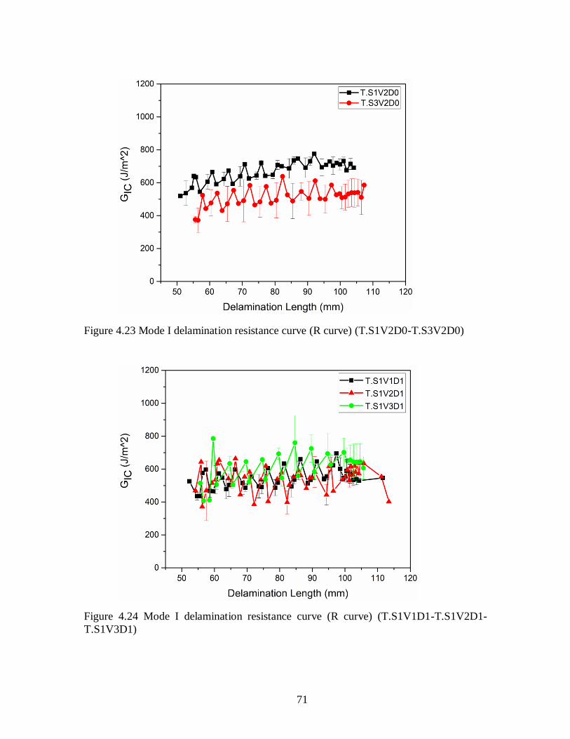
71
Figure 4.23 Mode I delamination resistance curve (R curve) (T.S1V2D0-T.S3V2D0)
Figure 4.24 Mode I delamination resistance curve (R curve) (T.S1V1D1-T.S1V2D1-
T.S1V3D1)

72
Figure 4.25 Mode I delamination resistance curve (R curve) (T.S2V1D1-T.S2V2D1-
T.S2V3D1)
Figure 4.26 Mode I delamination resistance curve (R curve) (T.S3V1D1-T.S3V2D1-
T.S3V3D1)
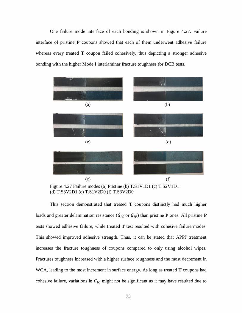
73
One failure mode interface of each bonding is shown in Figure 4.27. Failure
interface of pristine P coupons showed that each of them underwent adhesive failure
whereas every treated T coupon failed cohesively, thus depicting a stronger adhesive
bonding with the higher Mode I interlaminar fracture toughness for DCB tests.
(a) (b)
(c) (d)
(e) (f)
Figure 4.27 Failure modes (a) Pristine (b) T.S1V1D1 (c) T.S2V1D1
(d) T.S3V2D1 (e) T.S1V2D0 (f) T.S3V2D0
This section demonstrated that treated T coupons distinctly had much higher
loads and greater delamination resistance (𝐺𝐼𝐶 or 𝐺𝐼𝑃) than pristine P ones. All pristine P
tests showed adhesive failure, while treated T test resulted with cohesive failure modes.
This showed improved adhesive strength. Thus, it can be stated that APPJ treatment
increases the fracture toughness of coupons compared to only using alcohol wipes.
Fractures toughness increased with a higher surface roughness and the most decrement in
WCA, leading to the most increment in surface energy. As long as treated T coupons had
cohesive failure, variations in 𝐺𝐼𝐶 might not be significant as it may have resulted due to

74
failure initiations at different depths along the adherend. In such cases, treatment
parameters could be chosen on basis of duration and cost-effectiveness. In the present
case, combinations of S2 & V1 & D1 and S3 & V2 & D1 would also be expected to be
among the most cost-effective ones. Thus, either of these two combinations of treatment
parameters could be relied upon based on manufacturing convenience.

75
CONCLUSIONS AND FUTURE WORK
In this work, APPJ surface preparation method, which is a low-temperature,
reliable, automated, and environmentally benign plasma, has been experimented to
improve the adhesive bond strength of CFRPs, which were produced with IM7/8552
prepreg material. The effects of plasma treatment on composite material have been
analyzed with a water contact angle measurement called ballistic deposition method, XPS
for chemical modifications, and SEM and AFM for surface morphological and
topographical changes. The bond strength of pristine P and treated T composites has been
evaluated with the DCB test by calculating Mode I interlaminar fracture toughness
according to modified beam theory (𝐺𝐼𝐶) and area method (𝐺𝐼𝑃) and determining failure
modes.
5.1 CONCLUSION
The receding water contact angle with surface analyst device, which is used as an
estimation of surface energy, decreased following plasma treatment which indicated an
increase in surface energy and higher hydrophilicity. XPS results prior to and following
treatment has shown a noticeable decrease in carbon content and a significant increase in
oxygen content with enhanced oxygen-containing functional groups. The O/C ratio,
which is used for functionalization level, has shown an increase with treatment, and it
was the highest due to higher treatment duration for the slowest speed (S1), overlap 50%
76
(V2) at distance D0 (0.25 in). While all the samples have had predominantly SiC for
pristine, SiO2 has increased remarkably via plasma treatment which has shown oxidation
of silicon. SEM images have shown no visible damage on the carbon fibers themselves,
and plasma treatment has cleaned the surface from the impurities which prevent a
stronger bond. The higher surface roughness (rms) which indicates a higher adhesion was
measured for the treated T samples with AFM. DCB test results have proved that APPJ
treatment does have the potential to increase fracture toughness by the occurring cohesive
failure and improved bond consistency. Comparison of the fracture toughness has shown
around a three-time increase in 𝐺𝐼𝐶 and a twofold increase in 𝐺𝐼𝑃 for treated T samples.
Analysis of interfacial failures of the pristine P tests has had adhesive failures for all the
tests, whereas the treated T tests have had all cohesive failure modes which reflect
greater 𝐺𝐼𝑃 and 𝐺𝐼𝐶 values.
This increase on fracture toughness is a result of lower water contact angle, higher
O/C ratio, increased oxygen-functional groups, higher surface roughness and cleaned
surface contaminants.
5.2 FUTURE WORK
Future work could involve the use of various characterization techniques to
investigate the effect of atmospheric pressure plasma jet treatment on carbon fiber
reinforced polymers, in order to improve bond strength. For instance, Fourier Transform
Infrared (FTIR) Spectroscopy could be used to quantify the chemical changing on the
surface, and the results can be compared with those from XPS analysis.
Also, different variations of plasma process parameters could be used to examine
the plasma effects and determine Mode I interlaminar fracture toughness and failure
77
modes. For example, the use of higher treatment speeds with closer and further distances
from plasma jet to the composite surface could be investigated.
In addition, bondline thickness could be investigated on certain points, and the
maximum, minimum, and average value on the test coupon could be taken to figure out
its effects for cohesive failure modes and 𝐺𝐼𝐶 values.
Ultimately, silicon has been detected by XPS for the composite panels which
were tested in this study, but contamination process has not been included for this
research. Future work might be focused on the investigation of fracture toughness and the
plasma treatment effects with the produced composite panels, without an exposure to
silicon during the manufacturing process. The contamination process that results from the
presence of higher silicon amounts on composite samples has not been included in this
study. Composite panels can be contaminated and then treated before testing, or they can
be contaminated and tested without the treatment process.
5.3 SITUATION OF RESEARCH
Understanding the effects of surface preparation on AFP manufactured coupons
subscribe to an overall AFP research undertaken at the University of South Carolina’s
McNair Center. This research complements path planning studies for AFP [122-125]
where finding the optimal tool path for laying fibers is sought. One of the principal
conditions is the minimization of AFP defects [126, 127] and the effect they can have on
the integrity of the structure [128-130]. Efficient design processes [131, 132] and rapid
assessment tools [133] can practically support a better integral lay-up quality. This study
pushes the boundary to understand the composite behavior, when both efficient design
and manufacturing are used to obtain the laminate. This opens the possibility for design

78
to overcome the issues with mechanical joining of composites. To better illustrate the
goal, we will forward two design scenarios:
1) Adhesive bonding is not efficient and should not be used.
2) Adhesive bonding is efficient and can be used.
In scenario one, if a mechanical joints are needed at location 1 in Figure 5.1, the
lay-up strategy needs to account for that and possible solutions are Figure 5.1b&c.
(a) (b) (c)
Figure 5.1 Lay-up strategy considerations
In scenario two, since mechanical joints are not needed, we can relax the
concentration of reinforcement requirement of Figure 5.1b&c.
Finally, the composite lifecycle, currently not integrated, can profit by reducing
overall design constraints making solution finding easier similar to [134-135].
1
Concentration Build-up

79
REFERENCES
1. He, R., et al., Improved mechanical properties of carbon fiber reinforced PTFE
composites by growing graphene oxide on carbon fiber surface. Composite
Interfaces, 2018. 25(11): p. 995-1004.
2. Mishnaevsky, L. and G. Dai, Hybrid and hierarchical nanoreinforced polymer
composites: Computational modelling of structure–properties relationships.
Composite Structures, 2014. 117: p. 156-168.
3. Pendhari, S.S., T. Kant, and Y.M. Desai, Application of polymer composites in
civil construction: A general review. Composite Structures, 2008. 84(2): p. 114-
124.
4. Zhou, H.W., et al., Carbon fiber/carbon nanotube reinforced hierarchical
composites: Effect of CNT distribution on shearing strength. Composites Part B:
Engineering, 2016. 88: p. 201-211.
5. Boerio, F., et al., Effect of grit-blasting on the surface energy of graphite/epoxy
composites. The Journal of Adhesion, 2006. 82(1): p. 19-37.
6. Di Franco, G., L. Fratini, and A. Pasta, Influence of the distance between rivets in
self-piercing riveting bonded joints made of carbon fiber panels and AA2024
blanks. Materials & Design, 2012. 35: p. 342-349.
7. Encinas, N., et al., Surface modification of aircraft used composites for adhesive
bonding. International Journal of Adhesion and Adhesives, 2014. 50: p. 157-163.
8. Hegemann, D., H. Brunner, and C. Oehr, Plasma treatment of polymers for
surface and adhesion improvement. Nuclear instruments and methods in physics
research section B: Beam interactions with materials and atoms, 2003. 208: p.
281-286.
9. Tiwari, S. and J. Bijwe, Surface treatment of carbon fibers-a review. Procedia
Technology, 2014. 14: p. 505-512.
10. Banea, M. and L.F. da Silva, Adhesively bonded joints in composite materials: an
overview. Proceedings of the Institution of Mechanical Engineers, Part L: Journal
of Materials: Design and Applications, 2009. 223(1): p. 1-18.
11. Zaldivar, R., et al., The effect of atmospheric plasma treatment on the chemistry,
morphology and resultant bonding behavior of a pan-based carbon fiber-

80
reinforced epoxy composite. Journal of composite materials, 2010. 44(2): p. 137-
156.
12. Dillingham, R.G., B.R. Oakley, and D. Gilpin*, Wetting measurements for
identification of specific functional groups responsible for adhesion. The Journal
of Adhesion, 2008. 84(12): p. 1007-1022.
13. Anand, M., R.E. Cohen, and R.F. Baddour, Surface modification of low density
polyethylene in a fluorine gas plasma. Polymer, 1981. 22(3): p. 361-371.
14. Kim, M., et al., Surface treatment of metals using an atmospheric pressure
plasma jet and their surface characteristics. Surface and Coatings Technology,
2003. 174: p. 839-844.
15. Agostino, R., plasma Deposition. Treatment and Etching of Polymers, Academic,
Orlando, 1990.
16. Inagaki, N., Plasma surface modification and plasma polymerization. 1996: CRC
Press.
17. Greenwood, O.D., et al., Atmospheric silent discharge versus low-pressure
plasma treatment of polyethylene, polypropylene, polyisobutylene, and
polystyrene. Journal of Adhesion Science and Technology, 1995. 9(3): p. 311-
326.
18. Taylor, W., Technical synopsis of plasma surface treatments. University of
Florida, Gainesville, FL, 2009.
19. Dowling, D.P., et al., Influence of dc pulsed atmospheric pressure plasma jet
processing conditions on polymer activation. Plasma Processes and Polymers,
2011. 8(8): p. 718-727.
20. Jordá‐Vilaplana, A., et al., Improvement of mechanical properties of polylactic
acid adhesion joints with bio‐based adhesives by using air atmospheric plasma
treatment. Journal of Applied Polymer Science, 2015. 132(32).
21. Shenton, M. and G. Stevens, Surface modification of polymer surfaces:
atmospheric plasma versus vacuum plasma treatments. Journal of Physics D:
Applied Physics, 2001. 34(18): p. 2761.
22. Li, H., et al., Air dielectric barrier discharges plasma surface treatment of three-
dimensional braided carbon fiber reinforced epoxy composites. Surface and
Coatings Technology, 2009. 203(10-11): p. 1317-1321.
23. Van de Velde, K. and P. Kiekens, Wettability and surface analysis of glass fibres.
2000.

81
24. Tendero, C., et al., Atmospheric pressure plasmas: A review. Spectrochimica Acta
Part B: Atomic Spectroscopy, 2006. 61(1): p. 2-30.
25. Borcia, G., C. Anderson, and N. Brown, The surface oxidation of selected
polymers using an atmospheric pressure air dielectric barrier discharge. Part II.
Applied surface science, 2004. 225(1): p. 186-197.
26. Borcia, G., C.A. Anderson, and N.M.D. Brown, The surface oxidation of selected
polymers using an atmospheric pressure air dielectric barrier discharge. Part I.
Applied Surface Science, 2004. 221(1): p. 203-214.
27. Noh, B.-I., et al., Effect of plasma treatment on adhesion characteristics at
interfaces between underfill and substrate. International journal of adhesion and
adhesives, 2007. 27(3): p. 200-206.
28. McDaniel, D., et al. Effect of surface contamination on composite bond integrity
and durability. in Advanced Materials in Transport Aircraft Structures Autumn
2011 Meeting. 2011.
29. Lee, H., I. Ohsawa, and J. Takahashi, Effect of plasma surface treatment of
recycled carbon fiber on carbon fiber-reinforced plastics (CFRP) interfacial
properties. Applied Surface Science, 2015. 328: p. 241-246.
30. Xie, J., et al., Improving carbon fiber adhesion to polyimide with atmospheric
pressure plasma treatment. Surface and coatings technology, 2011. 206(2-3): p.
191-201.
31. Noeske, M., et al., Plasma jet treatment of five polymers at atmospheric pressure:
surface modifications and the relevance for adhesion. International journal of
adhesion and adhesives, 2004. 24(2): p. 171-177.
32. Bozaci, E., et al., Effects of the atmospheric plasma treatments on surface and
mechanical properties of flax fiber and adhesion between fiber–matrix for
composite materials. Composites Part B: Engineering, 2013. 45(1): p. 565-572.
33. Schutze, A., et al., The atmospheric-pressure plasma jet: a review and
comparison to other plasma sources. IEEE transactions on plasma science, 1998.
26(6): p. 1685-1694.
34. Gilpin, A.D., B.R. Oakley, and R.G. Dillingham, Water contact angle as a
quantitative measure of total polyethylene surface energy. Journal of Adhesion
Science and Technology, 2015. 29(9): p. 890-895.
35. Kusano, Y., Atmospheric pressure plasma processing for polymer adhesion: a
review. The Journal of Adhesion, 2014. 90(9): p. 755-777.

82
36. Kusano, Y., T.L. Andersen, and P. Michelsen. Atmospheric pressure plasma
surface modification of carbon fibres. in Journal of Physics: Conference Series.
2008. IOP Publishing.
37. Ashcroft, I., D. Hughes, and S. Shaw, Mode I fracture of epoxy bonded composite
joints: 1. Quasi-static loading. International Journal of Adhesion and Adhesives,
2001. 21(2): p. 87-99.
38. Blackman, B., et al., Measuring the mode I adhesive fracture energy, GIC, of
structural adhesive joints: the results of an international round-robin.
International journal of adhesion and adhesives, 2003. 23(4): p. 293-305.
39. Standard, A., D5528, 01 (2007) e3," Standard Test Method for Mode I
Interlaminar Fracture Toughness of Unidirectional Fiber-Reinforced Polymer
Matrix Composites. ASTM International, 2007.
40. De Moura, M., R. Campilho, and J. Gonçalves, Crack equivalent concept applied
to the fracture characterization of bonded joints under pure mode I loading.
Composites Science and Technology, 2008. 68(10-11): p. 2224-2230.
41. Andersson, T. and U. Stigh, The stress–elongation relation for an adhesive layer
loaded in peel using equilibrium of energetic forces. International Journal of
Solids and Structures, 2004. 41(2): p. 413-434.
42. Nairn, J.A., Energy release rate analysis for adhesive and laminate double
cantilever beam specimens emphasizing the effect of residual stresses.
International Journal of Adhesion and Adhesives, 2000. 20(1): p. 59-70.
43. Srinivas, S., Analysis of Bonded Joints. 1975, NATIONAL AERONAUTICS
AND SPACE ADMINISTRATION HAMPTON VA LANGLEY RESEARCH
CEN TER.
44. Fitton, M.D. and J. Broughton, Variable modulus adhesives: an approach to
optimised joint performance. International journal of adhesion and adhesives,
2005. 25(4): p. 329-336.
45. Da Silva, L.F. and R. Adams, Joint strength predictions for adhesive joints to be
used over a wide temperature range. International Journal of Adhesion and
Adhesives, 2007. 27(5): p. 362-379.
46. Da Silva, L.F. and R. Adams, Adhesive joints at high and low temperatures using
similar and dissimilar adherends and dual adhesives. International Journal of
Adhesion and Adhesives, 2007. 27(3): p. 216-226.
47. Hart-Smith, L., D. Brown, and S. Wong, Surface preparations for ensuring that
the glue will stick in bonded composite structures, in Handbook of Composites.
1998, Springer. p. 667-685.

83
48. Kutscha, E.O., et al., Contamination and Surface Preparation Effects on
Composite Bonding. 2017.
49. Crane, R., G. Dillingham, and B. Oakley, Progress in the Reliability of Bonded
Composite Structures. Applied Composite Materials, 2017. 24(1): p. 221-233.
50. Montes-Morán, M., et al., A study of the effect of plasma treatment on the
interfacial properties of carbon fibre–thermoplastic composites. Carbon, 2005.
43(8): p. 1795-1799.
51. Bubert, H., et al., Basic analytical investigation of plasma-chemically modified
carbon fibers. Spectrochimica Acta Part B: Atomic Spectroscopy, 2002. 57(10):
p. 1601-1610.
52. Dillingham, G., et al., Quantitative detection of peel ply derived contaminants via
wettability measurements. Journal of Adhesion Science and Technology, 2012.
26(10-11): p. 1563-1571.
53. Roth, J.R., Industrial Plasma Engineering: Volume 2-Applications to Nonthermal
Plasma Processing. Vol. 2. 2001: CRC press.
54. Mittal, K.L., Polymer surface modification: relevance to adhesion. Vol. 3. 2004:
CRC Press.
55. Cotter, J. and A. Mahoon, Development of new surface pretreatments, based on
alkaline hydrogen peroxide solutions, for adhesive bonding of titanium.
International Journal of Adhesion and Adhesives, 1982. 2(1): p. 47-52.
56. Kruse, A., et al., Surface pretreatment of plastics for adhesive bonding. Journal of
adhesion science and technology, 1995. 9(12): p. 1611-1621.
57. Molitor, P., V. Barron, and T. Young, Surface treatment of titanium for adhesive
bonding to polymer composites: a review. International Journal of Adhesion and
Adhesives, 2001. 21(2): p. 129-136.
58. Wu, S., Polymer interface and adhesion. 1982: M. Dekker.
59. Lommatzsch, U., et al., Atmospheric pressure plasma jet treatment of
polyethylene surfaces for adhesion improvement. Plasma Processes and Polymers,
2007. 4(S1).
60. Morent, R., et al., Non-thermal plasma treatment of textiles. Surface and coatings
technology, 2008. 202(14): p. 3427-3449.
61. Hanusová, J., et al., Atmospheric pressure plasma treatment of polyamide-12
foils. Open Chemistry, 2015. 13(1).

84
62. Van Deynse, A., R. Morent, and N. De Geyter, Surface modification of polymers
using atmospheric pressure cold plasma technology, in Polymer science: research
advances, pratical applications and educational aspects. 2016, Formatex
Research Center. p. 506-516.
63. Selwyn, G., et al., Materials processing using an atmospheric pressure, RF-
generated plasma source. Contributions to Plasma Physics, 2001. 41(6): p. 610-
619.
64. Tracey, A.C., Effect of Atmospheric Pressure Plasma Treatment on Surface
Characteristics and Adhesive Bond Quality of Peel Ply Prepared Composites.
2014.
65. Gerenser, L., Surface chemistry of plasma-treated polymers. 1996, IOP
Publishing, Bristol. p. 1.
66. Kumar, S., et al., Effect of atmospheric pressure plasma treatment for repair of
polymer matrix composite for aerospace applications. Journal of Composite
Materials, 2016. 50(11): p. 1497-1507.
67. Jie, S. and Q. Yiping, The effects of gas composition on the atmospheric pressure
plasma jet modification of polyethylene films. Plasma Science and Technology,
2015. 17(5): p. 402.
68. Murokh, I., Atmospheric Plasma Surface Treatment Technique. El Segundo, CA:
Tri-Star Technologies, 2005.
69. Yu, H., Application of atmospheric pressure plasma in polymer and composite
adhesion. 2016, University of California, Los Angeles.
70. Williams, T.S. and R.F. Hicks, Aging mechanism of the native oxide on silicon
(100) following atmospheric oxygen plasma cleaning. Journal of Vacuum Science
& Technology A: Vacuum, Surfaces, and Films, 2011. 29(4): p. 041403.
71. Flinn, B.D., et al., Improving Adhesive Bonding of Composites Through Surface
Characterization. The Joint Advanced Materials and Structures Center of
Excellence, CECAM, and AMTAS, University of Washington in: http://depts.
washington. edu/amtas/ev-ents/jams_, 2010. 8: p. 21.
72. Williams, T.S., Surface Modification by Atmospheric Pressure Plasma for
Improved Bonding. 2013: University of California, Los Angeles.
73. Fauchais, P. and A. Vardelle, Thermal plasmas. IEEE Transactions on plasma
science, 1997. 25(6): p. 1258-1280.
74. Smith, R., D. Wei, and D. Apelian, Thermal plasma materials processing—
Applications and opportunities. Plasma Chemistry and Plasma Processing, 1989.
9(1): p. 135S-165S.

85
75. Ramakrishnan, S. and M. Rogozinski, Properties of electric arc plasma for metal
cutting. Journal of Physics D: Applied Physics, 1997. 30(4): p. 636.
76. Yu, R.H., et al., Atmospheric and Vacuum Plasma Treatments of Polymer
Surfaces for Enhanced Adhesion in Microelectronics Packaging. Adhesion in
Microelectronics, 2014: p. 137-172.
77. Laroussi, M. and T. Akan, Arc‐free atmospheric pressure cold plasma jets: a
review. Plasma Processes and Polymers, 2007. 4(9): p. 777-788.
78. Elaragi, G. and H. Elaraby, Characterization of an Atmospheric-pressure Cold
Plasma Jet.
79. Chen, F.F. and J.P. Chang, Principles of plasma processing. Univ. of California,
book, 2002.
80. Babayan, S., et al., Characterization of the active species in the afterglow of a
nitrogen and helium atmospheric-pressure plasma. Plasma Chemistry and Plasma
Processing, 2002. 22(2): p. 255-269.
81. Kaelble, D., Dispersion-polar surface tension properties of organic solids. The
Journal of Adhesion, 1970. 2(2): p. 66-81.
82. Good, R.J., Contact angle, wetting, and adhesion: a critical review. Journal of
adhesion science and technology, 1992. 6(12): p. 1269-1302.
83. Jacobasch, H.-J., et al., Application of the surface free energy concept in polymer
processing. Journal of adhesion science and technology, 1992. 6(12): p. 1381-
1396.
84. Kwok, D., et al., Measuring and interpreting contact angles: a complex issue.
Colloids and Surfaces A: Physicochemical and Engineering Aspects, 1998. 142(2-
3): p. 219-235.
85. Tran, L.Q.N., et al., Wetting analysis and surface characterisation of coir fibres
used as reinforcement for composites. Colloids and Surfaces A: Physicochemical
and Engineering Aspects, 2011. 377(1): p. 251-260.
86. Yuan, Y. and T.R. Lee, Contact angle and wetting properties, in Surface science
techniques. 2013, Springer. p. 3-34.
87. Gao, L. and T. McCarthy, Wetting 101 Langmuir 2009, 25, 14105–14115. DOI.
88. Strobel, M., et al., Contact angle measurements on oxidized polymer surfaces
containing water-soluble species. Journal of Adhesion Science and Technology,
2015. 29(14): p. 1483-1507.

86
89. Thakker, M., et al., Validation of Low Cost Solid Liquid Contact Angle Instrument
Using Drop Shape Image Processing Suitable For Surface Property
Measurement. International Journal of Current Engineering and Technology,
2013. 3(3): p. 877-888.
90. Oporto, G.S., et al., Forced air plasma treatment (FAPT) of hybrid wood plastic
composite (WPC)–fiber reinforced plastic (FRP) surfaces. Composite Interfaces,
2009. 16(7-9): p. 847-867.
91. Van Deynse, A., et al., Surface modification of polyethylene in an argon
atmospheric pressure plasma jet. Surface and Coatings Technology, 2015. 276: p.
384-390.
92. Young, T., III. An essay on the cohesion of fluids. Philosophical transactions of
the royal society of London, 1805. 95: p. 65-87.
93. Pappas, D., C. Copeland, and R. Jensen, Wettability Tests of Polymer Films and
Fabrics and Determination of Their Surface Energy by Contact-Angle Methods.
2007, ARMY RESEARCH LAB ABERDEEN PROVING GROUND MD.
94. Fowkes, F.M., Additivity of intermolecular forces at interfaces. i. determination of
the contribution to surface and interfacial tensions of dispersion forces in various
liquids1. The Journal of Physical Chemistry, 1963. 67(12): p. 2538-2541.
95. Owens, D., Some thermodynamic aspects of polymer adhesion. Journal of applied
polymer science, 1970. 14(7): p. 1725-1730.
96. Goldstein, J.I., et al., Generation of X-rays in the SEM specimen, in Scanning
Electron Microscopy and X-Ray Microanalysis. 2003, Springer. p. 271-296.
97. Skoog, D.A., F.J. Holler, and S.R. Crouch, Principles of instrumental analysis.
2017: Cengage learning.
98. Slayter, E.M. and H.S. Slayter, Light and electron microscopy. 1992: Cambridge
University Press.
99. Ren, Y., C. Wang, and Y. Qiu, Aging of surface properties of ultra high modulus
polyethylene fibers treated with He/O2 atmospheric pressure plasma jet. Surface
and Coatings Technology, 2008. 202(12): p. 2670-2676.
100. Liu, Y., et al., Influence of environmental moisture on atmospheric pressure
plasma jet treatment of ultrahigh-modulus polyethylene fibers. Journal of
Adhesion Science and Technology, 2007. 21(8): p. 663-676.
101. Gao, Z., et al., Influence of processing parameters on atmospheric pressure
plasma etching of polyamide 6 films. Applied Surface Science, 2009. 255(17): p.
7683-7688.
87
102. Czabaj, M.W. and J.G. Ratcliffe, Comparison of intralaminar and interlaminar
mode I fracture toughnesses of a unidirectional IM7/8552 carbon/epoxy
composite. Composites Science and Technology, 2013. 89: p. 15-23.
103. Alfred Franklin, V. and T. Christopher, Fracture energy estimation of DCB
specimens made of glass/epoxy: an experimental study. Advances in Materials
Science and Engineering, 2013. 2013.
104. Prasad, M.S., C. Venkatesha, and T. Jayaraju, Experimental methods of
determining fracture toughness of fiber reinforced polymer composites under
various loading conditions. Journal of Minerals and Materials Characterization
and Engineering, 2011. 10(13): p. 1263.
105. Tracey, A., Improving Adhesive Bonding Through Surface Characterization:
Reverse the Curse of the Nylon Peel Ply. 2013. Boeing Co, 2013.
106. ASTM, D., 5573-99. Standard practice for classifying failure modes in fiber-
reinforced-plastic (FRP) joints. Annual book of ASTM standards, 2002. 15.
107. Shanahan, M. and C. Bourges-Monnier, Effects of plasma treatment on the
adhesion of an epoxy composite. International journal of adhesion and adhesives,
1996. 16(2): p. 129-135.
108. Navarro Rodriguez, B., Plasma pre-treatment for adhesive bonding of aerospace
composite components. 2016, Brunel University London.
109. Composites, H., HexPly® 8552 Product Data. 2000, Tech. Rep.(Hexcel, 2013).
110. Mathews, M.J. and S.R. Swanson, Characterization of the interlaminar fracture
toughness of a laminated carbon/epoxy composite. Composites Science and
Technology, 2007. 67(7-8): p. 1489-1498.
111. Huner, U., H.A. Gulec, and I. Damar Huner, Effect of gas type and application
distance on atmospheric pressure plasma jet-treated flax composites. Journal of
Reinforced Plastics and Composites, 2017. 36(17): p. 1197-1210.
112. Su, F.-h., et al., Tribological and mechanical properties of the composites made of
carbon fabrics modified with various methods. Composites Part A: Applied
Science and Manufacturing, 2005. 36(12): p. 1601-1607.
113. Cognard, J., Some recent progress in adhesion technology and science. Comptes
Rendus Chimie, 2006. 9(1): p. 13-24.
114. Luo, Y., et al., Surface and wettability property analysis of CCF300 carbon fibers
with different sizing or without sizing. Materials & Design, 2011. 32(2): p. 941-
946.

88
115. Payne, B., M. Biesinger, and N. McIntyre, X-ray photoelectron spectroscopy
studies of reactions on chromium metal and chromium oxide surfaces. Journal of
Electron Spectroscopy and Related Phenomena, 2011. 184(1-2): p. 29-37.
116. Fang, X., Jalowka, J., Riehl, J., Zhao, W., Goberman, D., Contamination effect on
composite-to-metal adhesive bond performance, in SAMPE Conference
Proceedings. 2017: Seattle, WA.
117. Fang, X., Sarao, G., Zhao, W., Goberman, D.G., Connell, J.W, Effectiveness of
Surface Treatment Techniques for Composite Bonding with Different
Contamination Levels, in SAMPE Conference Proceedings. 2018: Long Beach,
CA.
118. Webb, L.J., et al., High-resolution X-ray photoelectron spectroscopic studies of
alkylated silicon (111) surfaces. The Journal of Physical Chemistry B, 2005.
109(9): p. 3930-3937.
119. Birer, Ö., et al., XPS investigation of thin SiOx and SiOxNy overlayers. Journal of
molecular structure, 1999. 480: p. 611-614.
120. Encinas, N., et al., Extreme durability of wettability changes on polyolefin
surfaces by atmospheric pressure plasma torch. Surface and Coatings
Technology, 2010. 205(2): p. 396-402.
121. Encinas, N., et al., Atmospheric pressure plasma hydrophilic modification of a
silicone surface. The Journal of Adhesion, 2012. 88(4-6): p. 321-336.
122. Rousseau G, Wehbe R, Halbritter J, Harik R, Automated Fiber Placement Path
Planning: A state-of-the-art, review. Computer-Aided Design & Applications,
2019. 16(2): p. 172-203.
123. Noevere A, Collier C, Harik R, Halbritter J. Development of a Design for
Manufacturing Tool for Automated Fiber Placement Structures. in AIAA Scitech
2019 Forum. 2019.
124. Halbritter J, Harik R, Toren M, Waerdt W van de, Modular Conversion Tool For
Generating Fiber Placement Code From Optimized Fiber Steering Path, in The
Composites and Advanced Materials Expo CAMX2017. 2017.
125. Halbritter J, Harik R, Zuloaga A, Tooren M. Tool path generation on doubly-
curved free-form surfaces. Computer-Aided Design and Applications, 2017.
14(6): p. 844-851.
126. Harik R, Saidy C, Williams SJ, Gurdal Z, Grimsley B. Automated fiber placement
defect identity cards: cause, anticipation, existence, significance, and
progression. in Submission to SAMPE 2018 Conference & Exhibition, Long
Beach, California, US. 2018.

89
127. Rajan S, Sutton MA, Wehbe R, Tatting B, Gurdal Z, Kidane A, Harik R.
Experimental investigation of prepreg slit tape wrinkling during automated fiber
placement process using StereoDIC. Composites Part B: Engineering, 2019. 160:
p. 546-557.
128. Anay R, Ziehl P, Tessema A, Wehbe R, Assi L, Kidane A, Harik R, Tatting B,
Gurdal Z. An Experimental Investigation Concerning the Effects of AFP Defects
on Progressive Failure of Tensile Coupons. in AIAA Scitech 2019 Forum. 2019.
129. Wehbe R, Harik R, Gurdal Z. In-plane tow deformations due to steering in
automated fiber placement. in AIAA Scitech 2019 Forum. 2019.
130. Wehbe R, Harik R, Tatting B, Gurdal Z, Halbritter A, Wanthal S. Tow-Path
Based Modeling of Wrinkling During the Automated Fiber Placement Process.
The Composites and Advanced Materials Expo CAMX2017, 2017.
131. Albazzan M, Harik R, Tatting B, Gurdal Z. Efficient Design Optimization of
Nonconventional Laminated Composites using Lamination Parameters: A State of
the Art. Composite Structures, 209, pp 362-374
132. Sabido A, Bahamonde L, Harik R, Tooren M. Maturity assessment of the
laminate variable stiffness design process. Composite Structures, 2017. 160: p.
804-812.
133. Bahamonde L, Bazzan M, Chevalier P, Gurdal Z, Tatting B, Harik R. Rapid tools
for an AFP manufacturing defects assessment framework in SAMPE 2018
Conference & Exhibition. 2018: Long Beach, California, US.
134. Harik R, Shi Y, Baek S. Shape Terra: mechanical feature recognition based on a
persistent heat signature. Computer Aided Design and Applications, 2017. 14 (2)
pp 206-218
135. Harik R. Spécifications de fonctions pour un système d’aide à la génération
automatique de gamme d’usinage: application aux pièces aéronautiques de
structure, prototype logiciel dans le cadre du projet RNTL USIQUICK. Université
Henri Poincaré-Nancy I, 2007.
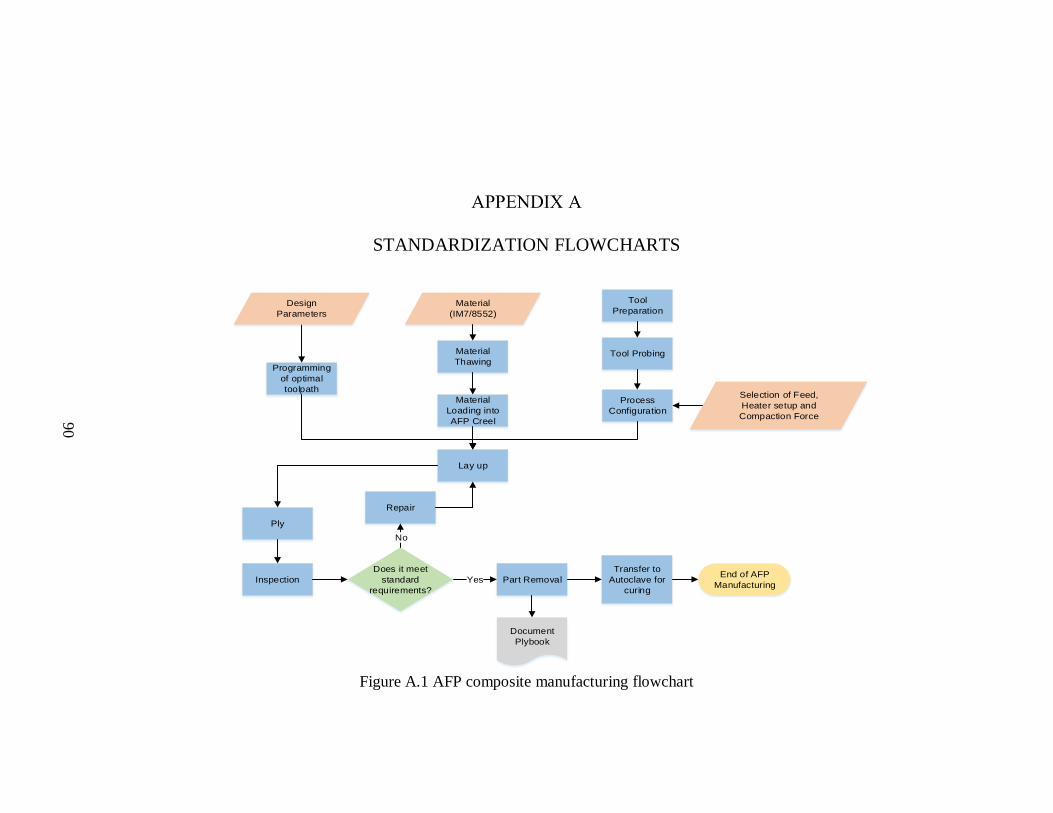
90
STANDARDIZATION FLOWCHARTS
Figure A.1 AFP composite manufacturing flowchart
Programming
of optimal
toolpath
Tool
Preparation
Tool Probing
Process
Configuration
Lay up
Ply
Inspection Part Removal
Repair
Material
Thawing
Material
Loading into
AFP Creel
End of AFP
Manufacturing
Does it meet
standard
requirements?
No
Yes
Document
Plybook
Transfer to
Autoclave for
curing
Selection of Feed,
Heater setup and
Compaction Force
Material
(IM7/8552)
Design
Parameters

91
Figure A.2 Autoclave cure cycle flowchart
Preparation
Is there any
pressure?
End of Autoclave Cure
Cycle
Open Door by verifying
depressurization of the
autoclave
A total vent is needed
which is done by
estopping the machine
Hold door close switch
until door is almost
closed, then pulse the
switch
Input appropriate
recipe
Press send recipe
Navigate to Main
Operations page, verify
cycle, and Start the
Cycle
Is the pressure less
than 5 psi?Yes No
Slowly move the
latching handle to open
position
Yes
Hold the lock/unlock
switch to unlock
position, open garage
door, and hold the door
open switch
Close Door after
placement of panel
Starting Curing
Is there an appropriate
recipe programmed?No
Yes
In an Emergency, press estop button
Once cycle complete,
and temp. & pressure
reach safe levels, open
door slowly
Allow material to set for
15 minutes after door
opening; remove
materials with insulated
gloves
Close and Secure
Autoclave Tightly;
Switch main power
disconnect off
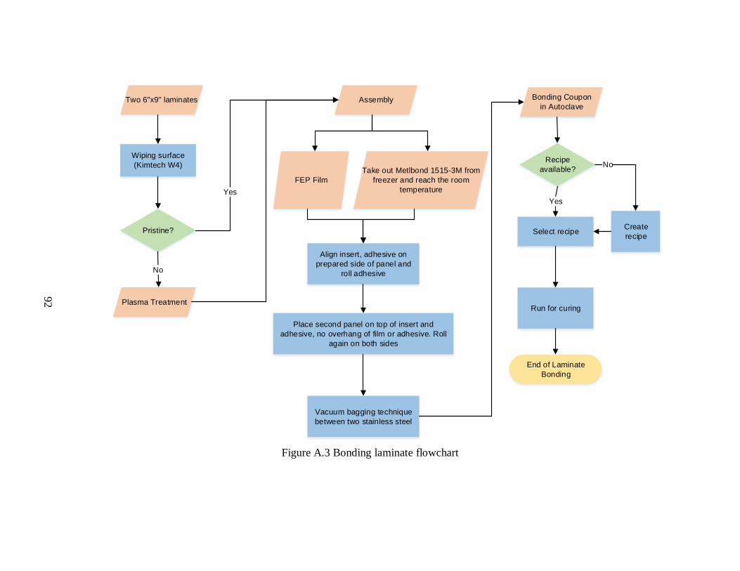
92
Figure A.3 Bonding laminate flowchart
Assembly
Align insert, adhesive on
prepared side of panel and
roll adhesive
Place second panel on top of insert and
adhesive, no overhang of film or adhesive. Roll
again on both sides
Vacuum bagging technique
between two stainless steel
FEP Film
Take out Metlbond 1515-3M from
freezer and reach the room
temperature
Bonding Coupon
in Autoclave
End of Laminate
Bonding
Two 6"x9" laminates
Pristine?
Plasma Treatment
Yes
No
Wiping surface
(Kimtech W4)Recipe
available?
Select recipe
Run for curing
Yes
Create
recipe
No

93
Figure A.4 Hinge bonding test flowchart
Cleaning with
acetone and alcohol
(hinge and
composite surface)
Sanding hinges Two Hinges Bonding with J-B
Weld
Clamping Hinges Curing
15-24 hours End of hinge bonding

94
Figure A.5 Atmospheric pressure plasma treatment flowchart
Turn on electrical
breaker
Turn air on
Turn on Plasma-Treat
machine
Set-up Specimen Configuration
Place specimen on XY
stage holder
Measure the distance from
nozzle to the surface of the
specimen
Set up software to run G-code
Upload grbl software to the
Arduino board using a hex
file
Plug in power supply
Select the hex file with an
Xloader software to
recognize the Arduino
board
Select the COM port which
the Arduino is plugged into
Open Universal G-code
sender
Run Code with Plasma
Once ready, start the flow of
plasma on the plasma-treat
Run G-code
simultaneously in pattern
that is needed for correct
speed and overlap
Close air valve, turn off
plasma treat machine, and
turn off electrical breaker
Set up Plasma-Treat
Do any faults
occur?
End of Plasma
Treatment
Turn off Plasma-Treat
machine and fix the
fault
Yes
No
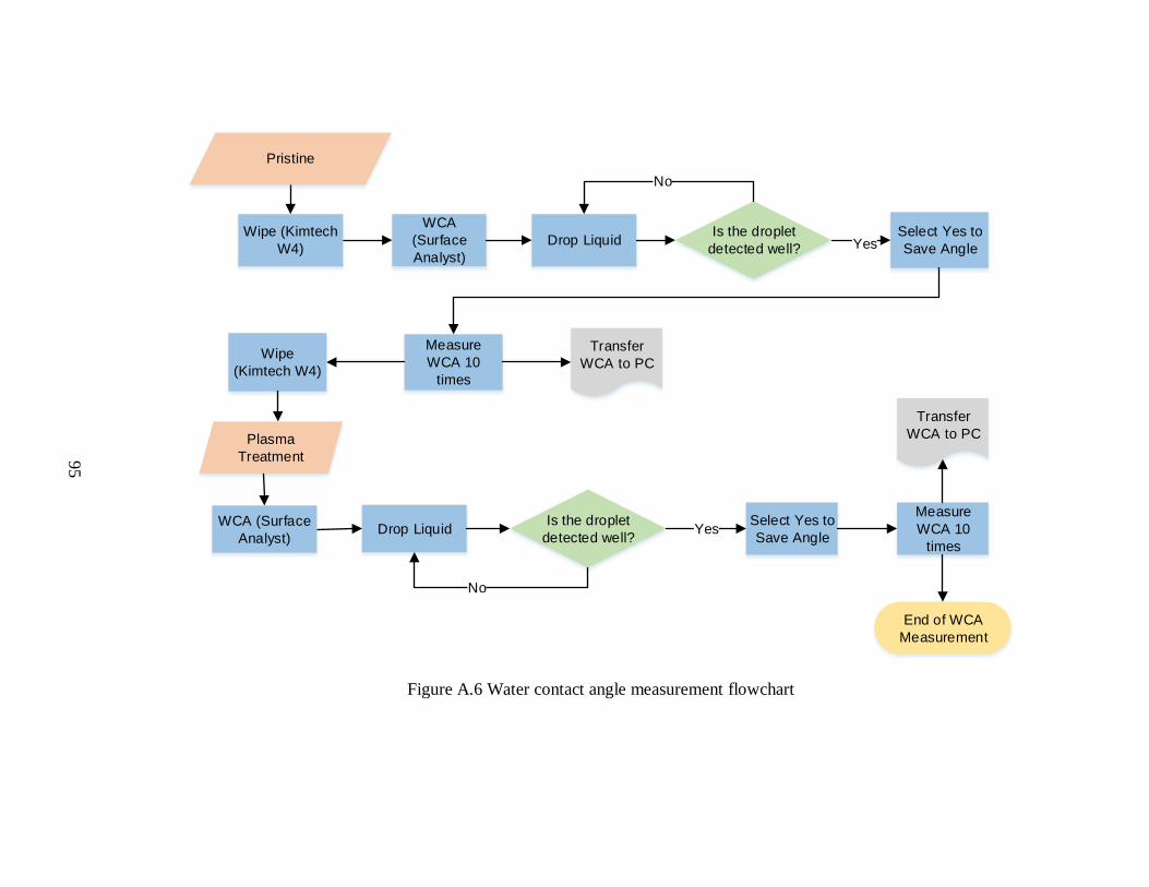
95
Figure A.6 Water contact angle measurement flowchart
WCA
(Surface
Analyst)
Drop LiquidSelect Yes to
Save Angle
Measure
WCA 10
times
Plasma
Treatment
Yes
Drop Liquid
Measure
WCA 10
times
End of WCA
Measurement
Wipe
(Kimtech W4)
WCA (Surface
Analyst)
Pristine
Wipe (Kimtech
W4)
Is the droplet
detected well?
No
Is the droplet
detected well?
No
Select Yes to
Save AngleYes
Transfer
WCA to PC
Transfer
WCA to PC
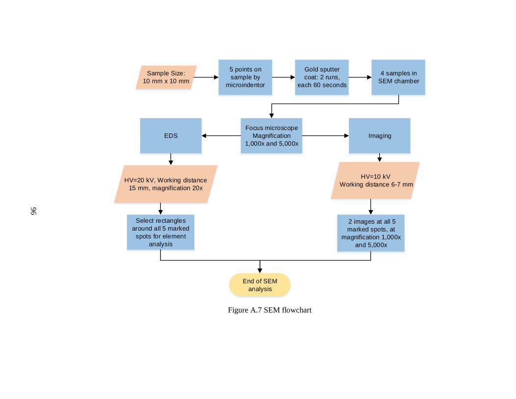
96
Figure A.7 SEM flowchart
Sample Size:
10 mm x 10 mm
Gold sputter
coat: 2 runs,
each 60 seconds
4 samples in
SEM chamber
Focus microscope
Magnification
1,000x and 5,000x
Imaging EDS
HV=20 kV, Working distance
15 mm, magnification 20x
2 images at all 5
marked spots, at
magnification 1,000x
and 5,000x
End of SEM
analysis
HV=10 kV
Working distance 6-7 mm
Select rectangles
around all 5 marked
spots for element
analysis
5 points on
sample by
microindentor

97
Figure A.8 Double cantilever beam test flowchart
Power on and unlock
handheld pad
Log into TW
Elite
Select standard tensile
test and input test
parameters
Adjust crossheads with
handheld pad until
Right click on load
indicator box and
select zero
Secure specimen is
MTS Grips
Make corrections by
adjusting crosshead grips
and re-aligning the
specimen
Once specimen is loaded, zero
the crossheads. DO NOT re-zero
the load indicator box this gives
false readings
Is handheld pad
unlocked?
Is specimen properlly
loaded? i.e (any twisting,
shifting, or slipping)
Is indicated load
reading approximately
0?
MTS Machine
Test Setup
Yes
No
No
Yes
No
Yes
Stop test and return to
zero once initial crack
length has reached 3-
5mm past end of insert
Run test 50 mm past
end of initial crack,
stop, and return to zero
Run test until specimen
failure Run DCB Test
Camera Setup
End of DCB Test