platform - utp press
TRANSCRIPT

P L A T F O R M
Volume 7 Number 1 Jan - Jun 2009
VOLUME SEVEN NUMBER ONE JANUARY - JUNE 2009 ISSN 1511-6794
PL
AT
FO
RM
VO
LU
ME
SE
VE
NN
UM
BE
RO
NE
JAN
UA
RY
-JU
NE
20
09
Mission-Oriented Research: DEEPWATER TECHNOLOGY
Numerical and Model Test Results for Truss Spar PlatformJohn V. Kurian, Osman A. A. Montasir, S.P. Narayanan
2
Mission-Oriented Research: ENHANCED OIL RECOVERY
Corncob And Sugar Cane Waste As A Viscosi� er In Hydrocarbon Drilling FluidSonny Irawan, Ahmad Zakuan Ahmad Azmi, Ismail Mohd. Saaid
9
Mission-Oriented Research: GREEN TECHNOLOGY
Analysis Of The Residence Time Distribution Of Solids In A Swirling Fluidised Bed Vijay R. Raghavan, Marneni Narahari
15
Technology Platform: APPLICATION OF INTELLIGENT IT SYSTEM
E-Learning's Discussion Room Impacts On Students Performance: A Case Study Of A System Analysis And Design CourseAliza Sarlan, Rohiza Ahmad, Wan Fatimah Wan Ahmad
22
Performance Appraisal System Using Multifactorial Evaluation ModelC.C. Yee, Chen Yoke Yie
28
Using Ontology For The Development Of Knowledge-Based System For E&P BusinessAinol R. Shazi, Mazeyanti M Ari� n, Fatihah Kasim
35
Missing Attribute Value Prediction Based On Arti� cial Neural Network And Rough Set TheoryN.A. Setiawan, P.A. Venkatachalam, Ahmad Fadzil Mohd Hani
42
Technology Platform: FUEL COMBUSTION
Burning Rates Of Turbulent Gaseous And Aerosol FlamesShaharin A. Sulaiman, Malcolm Lawes
48
Technology Platform: OFFSHORE EXPLORATION
Paleozoic Sedimentary Sequences Exposed In The Kinta Valley: Possible Clues To A Paleozoic Hydrocarbon System In And Around Peninsular Malaysia?Bernard J. Pierson, Askury A.Kadir, Chow Weng Sum, Zuhar Z.T. Harith
56
Technology Platform: RESERVOIR ENGINEERING
E� ects Of Mass Transfer And Free Convection Currents On The Flow Past An In�nite Vertical Plate With Ramped Wall TemperatureNarahari Marneni, O. Anwar Bég
66
Technology Platform: SYSTEM OPTIMISATION
Inherent Safety Index Module (ISIM) To Assess Inherent Safety Level During Preliminary Design StageChan T. Leong, Azmi Mohd Shari�
73
A Computational Procedure For Systematic Analysis Of Water Reuse, Regeneration And Recycle In Retro� t Design Of Re� nery Water Network SystemsKhor Cheng Seong
82
A Comparison Between MPC And PI Controllers Acting On A Refrigerated Gas PlantNooryusmiza Yuso� , M. Ramasamy
89

1 VOLUME SEVEN NUMBER ONE JANUARY - JUNE 2009 PLATFORM
I S S N 1 5 1 1 - 6 7 9 4
Contents
Copyright © 2009Universiti Teknologi PETRONAS
PLATFORMJanuary-June 2009
Advisor: Datuk Dr. Zainal Abidin Haji Kasim
PLATFORM Editorial
Editor-in-Chief:Prof. Ir. Dr. Ahmad Fadzil Mohd. Hani
Co-Editors:Assoc. Prof. Dr. Isa Mohd Tan
Assoc. Prof. Dr. Victor Macam Jr.
Assoc. Prof. Dr. Patthi Hussin
Dr. Baharum Baharuddin
Dr. Nor Hisham Hamid
Dr. Shahrina Mohd. Nordin
Subarna Sivapalan
Sub-Editor:Haslina Noor Hasni
UTP Publication Committee
Chairman: Dr. Puteri Sri Melor
Members: Prof. Ir. Dr. Ahmad Fadzil Mohamad Hani
Assoc. Prof. Dr. Madzlan Napiah
Assoc. Prof. Dr. M. Azmi Bustam
Dr. Nidal Kamel
Dr. Ismail M. Saaid
Dr. M. Fadzil Hassan
Dr. Rohani Salleh
Rahmat Iskandar Khairul Shazi Shaarani
Shamsina Shaharun
Anas M. Yusof
Haslina Noor Hasni
Roslina Nordin Ali
Secretary:Mohd. Zairee Shah Mohd. Shah
Address:PLATFORM Editor-in-Chief
Universiti Teknologi PETRONAS
Bandar Seri Iskandar, 31750 Tronoh
Perak Darul Ridzuan, Malaysia
http://www.utp.edu.my
[email protected]@petronas.com.my
Telephone +(60)5 368 8239
Facsimile +(60)5 365 4088
Mission-Oriented Research: DEEPWATER TECHNOLOGY
Numerical And Model Test Results For Truss Spar PlatformJohn V. Kurian, Osman A. A. Montasir, S.P. Narayanan
2
Mission-Oriented Research: ENHANCED OIL RECOVERY
Corncob And Sugar Cane Waste As A Viscosifier In Hydrocarbon Drilling FluidSonny Irawan, Ahmad Zakuan Ahmad Azmi, Ismail Mohd. Saaid
9
Mission-Oriented Research: GREEN TECHNOLOGY
Analysis Of The Residence Time Distribution Of Solids In A Swirling Fluidised Bed Vijay R. Raghavan, Marneni Narahari
15
Technology Platform: APPLICATION OF INTELLIGENT IT SYSTEM
E-Learning's Discussion Room Impacts On Students Performance: A Case Study Of A System Analysis And Design CourseAliza Sarlan, Rohiza Ahmad, Wan Fatimah Wan Ahmad
22
Performance Appraisal System Using Multifactorial Evaluation ModelC.C. Yee, Chen Yoke Yie
28
Using Ontology For The Development Of Knowledge-Based System For E&P BusinessAinol R. Shazi, Mazeyanti M Ariffin, Fatihah Kasim
35
Missing Attribute Value Prediction Based On Artificial Neural Network And Rough Set TheoryN.A. Setiawan, P.A. Venkatachalam, Ahmad Fadzil Mohd Hani
42
Technology Platform: FUEL COMBUSTION
Burning Rates Of Turbulent Gaseous And Aerosol Flames Shaharin A. Sulaiman, Malcolm Lawes
48
Technology Platform: OFFSHORE EXPLORATION
Paleozoic Sedimentary Sequences Exposed In The Kinta Valley: Possible Clues To A Paleozoic Hydrocarbon System In And Around Peninsular Malaysia?Bernard J. Pierson, Askury A.Kadir, Chow Weng Sum, Zuhar Z.T. Harith
56
Technology Platform: RESERVOIR ENGINEERING
Effects Of Mass Transfer And Free Convection Currents On The Flow Past An Infinite Vertical Plate With Ramped Wall TemperatureNarahari Marneni, O. Anwar Bég
66
Technology Platform: SYSTEM OPTIMISATION
Inherent Safety Index Module (ISIM) To Assess Inherent Safety Level During Preliminary Design StageChan T. Leong, Azmi Mohd Shariff
73
A Computational Procedure For Systematic Analysis Of Water Reuse, Regeneration And Recycle In Retrofit Design Of Refinery Water Network SystemsKhor Cheng Seong
82
A Comparison Between MPC And PI Controllers Acting On A Refrigerated Gas PlantNooryusmiza Yusoff, M. Ramasamy
89
2 PLATFORM VOLUME SEVEN NUMBER ONE JANUARY - JUNE 2009
Mission-Oriented Research: DEEPWATER TECHNOLOGY
This paper was presented at the Conference of ISOPE 2009 (International Society of Offshore and Polar Engineers), Japan, 21 - 26 June 2009
NUMERICAL AND MODEL TEST RESULTS FOR TRUSS SPAR PLATFORM
John V. Kurian*, Osman A. A. Montasir, S.P. NarayananUniversiti Teknologi PETRONAS, 31750 Tronoh, Perak Darul Ridzuan, Malaysia
ABSTRACT
A truss spar model was tested using regular waves in a wave basin and the responses in surge, heave and pitch were measured. A MATLAB program named ‘TRSPAR’ was developed to determine the responses by numerical method. This program was run using the model parameters and it gave results which agreed well with the corresponding results obtained from the test measurements. This program was then applied to a prototype spar, named Marlin truss spar. The simulated results were compared with the corresponding numerical results and test measurements.
Keywords: truss spar, responses, waves, model test, simulation.
INTRODUCTION
The spar platforms for offshore oil exploration and production in deep and ultra deep waters are increasingly becoming popular. A number of concepts have evolved, among them the ‘classic’ spar and ‘truss’ spar being the most prevalent. The classic spar has an upper buoyant cylindrical hard tank, a keel ballast tank (soft tank) and a flooded cylindrical midsection. The long midsection has a large diameter and its design is mostly governed by construction loads. As such, it is very cost-ineffective. In the late 1990s, development of truss spar concept advanced much with a large amount of research effort in model tests (Prislin et al. 1998, Troesch et al. 2000), and theoretical study (Kim et al. 1999, Luo et al. 2001, Wang et al. 2002). Since then, ten truss spars have been designed, constructed and/or installed.
The truss spar consists of a top hard tank and a bottom soft tank separated by a truss midsection. The soft tank mainly contains solid ballast to provide stability, whereas the hard tank provides buoyancy
and contains trim ballast. The truss section contains a number of horizontal heave plates designed to reduce heave motion by increasing both added mass and hydrodynamic damping.
Several analytical or numerical approaches can be used to calculate the dynamic response of spars. The most direct approach is the analysis in the time domain, where a wave elevation time series is used as input and the resulting structural responses are calculated numerically. In the structural analysis, it is common practice to treat the mooring lines and risers as springs. This neglects the inertia of the mooring system, as well as the additional drag forces that may increase the damping of the total structure.
A truss spar model of scaling factor 1:73, restrained by four horizontal mooring lines, was tested using regular waves in a wave basin 120 m long and 4 m wide with a water depth of 2.5 m. The responses in surge, heave and pitch were measured. A MATLAB program named ‘TRSPAR’ was developed to determine the responses. Time domain integration

3 VOLUME SEVEN NUMBER ONE JANUARY - JUNE 2009 PLATFORM
Mission-Oriented Research: DEEPWATER TECHNOLOGY
using Newmark Beta method was employed and the platform was modeled as a rigid body with six degrees of freedom restrained by mooring lines affecting the stiffness values. Wheeler stretching formula and modified Morison equation were used for simulating the sea state and for determining the dynamic force vector. Added mass and damping were derived from hydrodynamic considerations. The accuracy of this program was verified by comparison with both a set of laboratory model test results and a set of numerical analysis results reported in the literature.
EXPERIMENTS ON THE MODEL IN THE WAVE BASIN
The Model
The model was designed based on the dimensions of a typical existing spar with a scale ratio of 1:73 and was fabricated using galvanized steel. It comprised of two main sections; a conventional spar-shaped upper hull, and a lower truss section, as shown in Figure 1. The hull was 442 mm in diameter and 917 mm deep. The lower part of the spar was ballasted with water to bring the spar to a draft of 1.79 m. The truss was made up of three standard 312 × 312 × 312 mm bays, two 13 × 442 × 442 mm heave plates and a soft tank of 146 × 442 × 442 mm. The legs were 25 mm diameter
and the horizontal and diagonal structural elements were 10 mm in diameter. The total length of the truss part was 1.021 m.
Experimental Set-Up
The experiments were carried out in the Marine Technology Laboratory of University Technology Malaysia (UTM) at Skudai, Johor Baru. The basin was 120 m long and 4 m wide. The depth of the basin was 2.5 m. The waves were generated by a hydraulically driven flap type wave maker capable of generating waves up to a maximum height of 440 mm and a wave period less than 2.5 s. A beach at the far end of the basin absorbed the waves. The model test arrangement is shown in Figure 2, showing the horizontal soft mooring system comprising of four wires attached to linear springs. Within the constraints of the mooring system, the model was free to respond to the wave loading in all six degrees of freedom.
The wave environment was monitored with wave probes on the upstream side of the model. The responses were measured with two accelerometers fitted on the deck and at the CG of the model. Tensions in the wires were measured with four linear strain gauge type force transducers.
Experimental Program
Static Offset Test
This experiment was conducted to estimate the stiffness of the mooring lines. The model was pulled horizontally from the downstream side and then released to allow for the free vibration to die down. Readings from the transducers were recorded. The nonlinearity of the force-displacement relationship of the mooring lines was modeled using multi-linear segments with different slopes (stiffness) as shown in Figure 3.
Decay Test
Decay tests were conducted to calculate the damping ratio and the natural periods of the system in surge
Figure 1. Truss spar model (Scale: 1:73)

4 PLATFORM VOLUME SEVEN NUMBER ONE JANUARY - JUNE 2009
Mission-Oriented Research: DEEPWATER TECHNOLOGY
heave and pitch. The model was given an initial displacement and the subsequent motions were recorded. The results are shown in Table 1.
Table 1. Natural periods of vibration of the model
Motion Type Natural Period (sec)
Heave 2.468
Surge 2.414
Pitch 2.531
Regular Waves Tests
Table 2 summarises part of regular waves that were created for this experiment. Each regular wave test was run for a period of 1.5 min.
Table 2. Wave height and period of regular waves used for testing
Wave Height (cm) Wave Period (sec)
5.48 0.94
6.98 1.05
8.16 1.53
5.52 1.64
2.68 1.67
7.02 1.86
5.84 2
NUMERICAL MODEL
The nonlinear time domain numerical model performed step-by-step numerical integration of the exact large amplitude equation of motion, producing time histories of motions. The fluid forces on individual members were computed by the modified Morison equation in which the integration of the forces was performed over the instantaneous wetted length. The total force at each time step was obtained by summing the forces on the individual members. Incident wave kinematics was calculated by using Wheeler stretching formula. The mooring
(a) Section view
(b) Top view
Figure 2. Model test arrangement in the wave basin
Figure 3. Force-displacement relationship of the mooring lines
5 VOLUME SEVEN NUMBER ONE JANUARY - JUNE 2009 PLATFORM
Mission-Oriented Research: DEEPWATER TECHNOLOGY
system was modeled as weightless springs, affecting the stiffness values. A numerical model for a truss spar was developed that was able to predict the dynamic responses at any instant.
Considering that the incident waves were long crested and were advancing in the x-direction, the truss spar was approximated by a rigid body of three degrees of freedom (surge, heave and pitch), deriving static resistance from support systems (mooring lines) and hydrostatic stiffness.
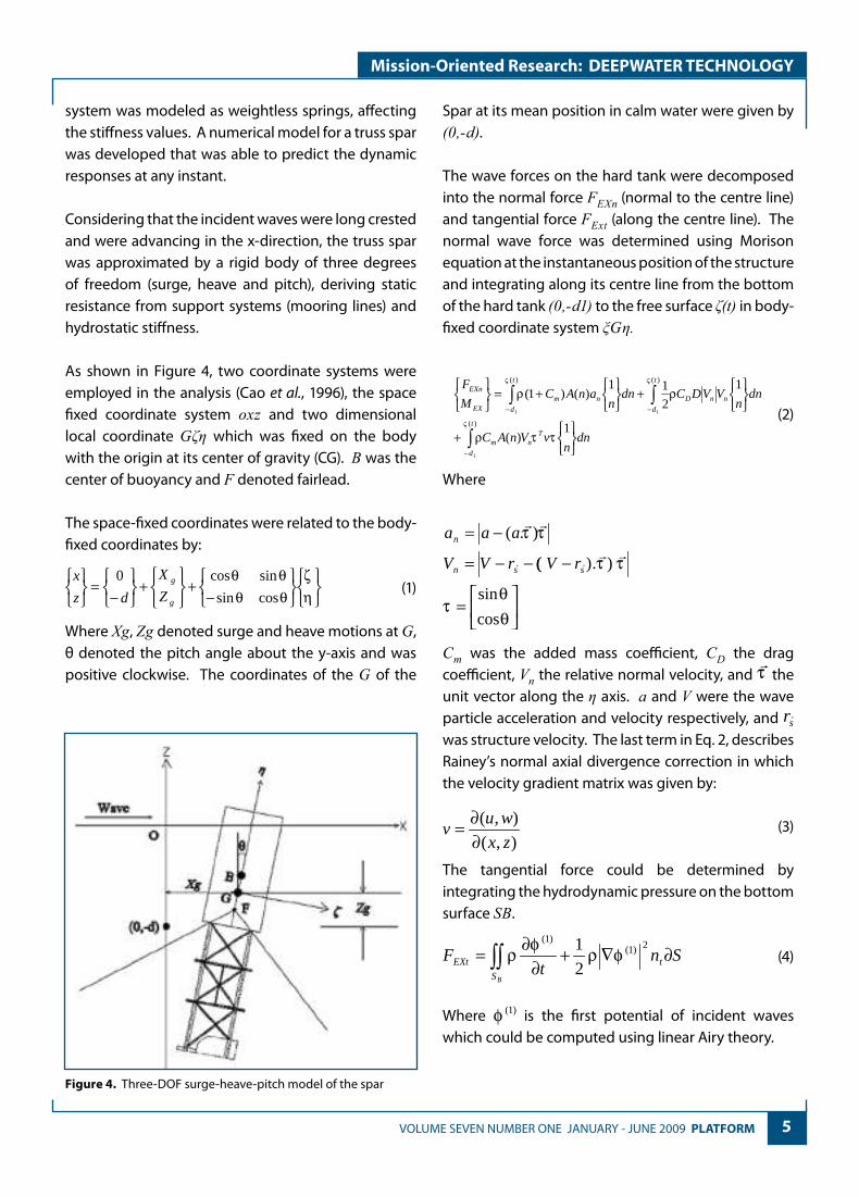
As shown in Figure 4, two coordinate systems were employed in the analysis (Cao et al., 1996), the space fixed coordinate system oxz and two dimensional local coordinate Gζη which was fixed on the body with the origin at its center of gravity (CG). B was the center of buoyancy and F denoted fairlead.
The space-fixed coordinates were related to the body-fixed coordinates by:
−
+
+
−
=
ηζ
θθθθ
cossin
sincos0
g
g
Z
X
dz
x (1)
Where Xg, Zg denoted surge and heave motions at G, θ denoted the pitch angle about the y-axis and was positive clockwise. The coordinates of the G of the
Spar at its mean position in calm water were given by (0,-d).
The wave forces on the hard tank were decomposed into the normal force FEXn (normal to the centre line) and tangential force FExt (along the centre line). The normal wave force was determined using Morison equation at the instantaneous position of the structure and integrating along its centre line from the bottom of the hard tank (0,-d1) to the free surface ζ(t) in body-fixed coordinate system ξGη.
dnn
vVnAC
dnn
VVDCdnn
anACM
F
Tn
t
d
m
nnD
t
d
n
t
d
mEX
EXn
+
+
+=
∫
∫∫
−
−−
1)(
1
2
11)()1(
)(
)()(
1
11
ττρ
ρρ
ς
ςς
(2)
Where
=
−−−=
−=
θθ
τ
ττ
ττ
cos
sin
)) .((
).(
..rr
rr
ssn
n
rVrVV
aaa
Cm was the added mass coefficient, CD the drag coefficient, Vn the relative normal velocity, and τ
r the
unit vector along the η axis. a and V were the wave particle acceleration and velocity respectively, and .
sr was structure velocity. The last term in Eq. 2, describes Rainey’s normal axial divergence correction in which the velocity gradient matrix was given by:
),(
),(
zx
wuv
∂∂= (3)
The tangential force could be determined by integrating the hydrodynamic pressure on the bottom surface SB.
Snt
F t
S
EXt
B
∂∇+∂
∂= ∫∫2)1(
)1(
2
1 φρφρ (4)
Where )1(φ is the first potential of incident waves which could be computed using linear Airy theory.
Figure 4. Three-DOF surge-heave-pitch model of the spar

6 PLATFORM VOLUME SEVEN NUMBER ONE JANUARY - JUNE 2009
Mission-Oriented Research: DEEPWATER TECHNOLOGY
Forces FEXn and FExt were transferred into spaced-fixed coordinate system oxz as:
−
=
EXt
EXn
EXz
EXx
F
F
F
F
θθθθ
cossin
sincos (5)
The equation of motion was solved by an iterative procedure using unconditionally stable Newmark’s Beta method.
The program ‘TRSPAR’ included a provision for calculating the values of drag and inertia hydrodynamic coefficients at any point of the structure and at any instant, based on the KC (Keulegan-Carpenter) parameter. The charts provided by (Chakrabarti, 2001) based on wave tank tests done on a cylinder, have been made use of. This provision was made use of for the numerical results of the model.
COMPARISON OF RESULTS
The responses of the truss spar model were determined numerically using the model parameters and the results were compared with the corresponding experimental values. The model dimensions, properties and draft were used. The wave heights and wave periods corresponding to the generated waves in the basin were used for evaluating the wave force on the numerical model. All response results presented in this paper were with respect to the G.
The Response Amplitude Operators (RAOs) for surge, heave and pitch of the numerical model were compared with experimental results in Figures 5-7. The RAOs were determined as the ratio of response heights to wave heights.
As could be seen, the RAOs for surge, heave and pitch motions were fairly well predicted by the numerical model. The trend of the surge RAO agreed well with the measured values with 20% higher values for the frequency range 3-7 rad/s. The heave RAOs agreed very well. For the pitch RAO, the simulation results followed the same trend as experimental results but it gave much lower values in wave frequencies between 3-6 rad/sec.
Figure 5. Comparison of surge motion RAO
Figure 6. Comparison of heave motion RAO
Figure 7. Comparison of pitch motion RAO

7 VOLUME SEVEN NUMBER ONE JANUARY - JUNE 2009 PLATFORM
Mission-Oriented Research: DEEPWATER TECHNOLOGY
This program ‘TRSPAR’ was then applied to a prototype structure, namely Marlin truss spar (Datta et.al., 1999) and the results were compared with the corresponding results computed using a Time Domain numerical simulation code called TDSIM (Paulling et al., 1995) and model test measurements. These comparisons are shown in Figures 8- 10.
The surge RAOs agreed very well as shown in Fig 8. The heave RAO for the ‘TRSPAR’ gave higher values compared to both the model test values and the TDSIM for the wave period range 12-25 s.
CONCLUSIONS
1) Available literature on the measured responses of truss spar models subjected to waves in wave basins, are only very few and this paper reports such a model study on a truss spar and compares with numerical results.
2) A MATLAB numerical program namely ‘TRSPAR’ was developed to determine the dynamic responses of a truss spar acted upon by regular waves.
3) ‘TRSPAR’ has provision for calculating the hydrodynamic coefficients at any point of the structure and at any instant, based on the KC parameter. This provision was made use of for
obtaining the numerical motion responses of the model.
4) The responses obtained using ‘TRSPAR’ were compared with the results of model tests conducted in a wave flume. Except for some differences in the surge and pitch amplitudes for the frequency range 3-7 rad/s, the trends and the magnitudes of the response RAOs agreed well.
5) The above program ‘TRSPAR’ was applied to a proto type spar namely Marlin truss spar and the responses compared with results of another numerical simulation called TDSIM and model
Figure 8. Comparison of surge RAO at zero degree heading Figure 9. Comparison of heave RAO at zero degree heading
Figure 10. Comparison of pitch RAO at zero degree heading

8 PLATFORM VOLUME SEVEN NUMBER ONE JANUARY - JUNE 2009
Mission-Oriented Research: DEEPWATER TECHNOLOGY
tests on this spar. Except for some differences in the heave response amplitude for the wave period range 12-25 s, all the three sets of results agreed well.
ACKNOWLEDGEMENTSThe support provided by the Universiti Teknologi PETRONAS and the Universiti Technologi Malaysia are gratefully acknowledged.
REFERENCES
[1] Cao, P.M., 1996, “Slow Motion Responses of Compliant Offshore Structures,” MS Thesis, Ocean Engineering Program, Civil Engineering Department, Texas A&M University, College Station, Texas.
[2] Chakrabati, S.K., 2001, “Hydrodynamics of Offshore Structures,” Computational Mechanics Publications, Southampton, Boston.
[3] Datta, I., Prislin, I., Halkyard, J.E., Greiner, W.L., Bhat, S., Perryman.S., and Beynet PA, 1999, “Comparison of Truss Spar Model Test Results with Numerical Predictions,” Proc 18th OMAE Conference, Newfoundland, Canada.
[4] Kim, M.H., Ran, R., Zheng, W., Bhat, S., and Beynet, P., 1999, “Hull/Mooring Coupled Dynamic Analysis of a Truss Spar in Time Domain,” Proc 9th Intl Offshore and Polar Eng, ISOPE, Brest, France.
[5] Luo, Y.H., Lu, R., Wang, J., and Berg S., 2001, “Time-Domain Fatigue Analysis for Critical Connections of Truss Spar,” Proc 11th Intl Offshore and Polar Eng, ISOPE, Stavanger, Vol 1, pp 362-368.
[6] Paulling, J.R., 1995, “TDSIM6: Time Domain Platform Motion Simulation with Six Degrees of Freedom. Theory and User Guide,” 4th Ed.
[7] Prislin, I., Belvins, R.D., and Halkyard, J.E., 1998, “Viscous Damping and Added Mass of Solid Square Plates.” Proc 17th OMAE Conference, Lisbon, Portugal.
[8] Troesch, A.W., Perlin, M., and He, H., 2000, “Hydrodynamics of Thin Plates,” Joint Industry Report, U. Michigan, Dept Naval Architecture and Marine Engineering, Ann Arbor.
[9] Wang, J., Luo, Y.H., and Lu, R. , 2002, “Truss Spar Structural Design for West Africa Environment,” Proc. 21st OMAE Conference, Oslo, Norway.
Dr Kurian V. John, BSc (Eng) (India) – Civil Engineering (1967), MTech (IIT Madras) – Structural Engineering (1972), PhD (IIT Madras) – Offshore Structures (1994), Life Member – MIE, MISTE. Total Experience – 41 years: Site Engineer, Skanska, Sultanate of Oman; Head of Civil Engineering, Federal Polytechnic Idah, Nigeria; Professor, NIT Calicut, India; Assoc.
Professor, UMS Kota Kinabalu; Assoc. Professor, UTP Tronoh. Publications – 90. PG Supervision – 24. Reviewer of International Journals, Conference Papers. Research Projects – 14 projects totaling RM1.5 million. Consultancy Projects – Many projects totaling RM0.5 million.
Montasir Osman graduated in Civil Engineering from Sudan University of Science and Technology in 1999, MSc in Structures from University of Khartoum in 2004. He worked as Engineer for few contracting and consulting firms from 2004 to 2006 before he joined University of Gezira as Lecturer. From there, he obtained study leave and joined UTP in
2007 for pursuing PhD. His research topic is ‘Analytical and Experimental Investigations on the Behaviour of Truss Spar Platforms’.
Narayanan S. P. was born in Trivandrum, India and acquired PhD in Civil Engineering from IIT Madras, India in 1998 for the work “Improving Cyclone Resistant Characteristics of Roof Cladding of Industrial Sheds”. His research is in the areas of steel and composite structures, and construction management. He worked as Senior Lecturer, TKM College of
Engineering (1990-2004), Associate Professor, Universiti Malaysia Sabah (2004-2007) and Universiti Teknologi PETRONAS (2007-till to date) and published over 70 papers in conferences and journals and three books. He conducted a sponsored course on “Disaster Mitigation – An Update for Civil Engineers”. Dr Narayanan is a life member of the IE (India) and ISTE.

9 VOLUME SEVEN NUMBER ONE JANUARY - JUNE 2009 PLATFORM
Mission-Oriented Research: ENHANCED OIL RECOVERY
INTRODUCTION
Oil and gas wells are drilled through different formations that require different mud properties to achieve optimum penetrations and stable borehole conditions. Therefore the design of a particular mud programme needs to consider a number of factors such as availability of additives, temperature and contamination. Protection of the environment is an important global issue and one that has been dominating development in the drilling fluids sector of the oil industry for some time. Legislation now exists in many countries which allows national or local authorities to regulate the discharge of chemicals and cuttings, usually via permit or license (McKee, 1995).
Generally, drilling fluids are classified into two categories; water based fluids (WBF) and non-aqueous based fluid (NABF). NABF can be divided into
three subcategories, oil based fluids (OBF), enhanced mineral oil based fluids (EMOBF) and synthetic based fluids (SBF). NABF has been widely used because of its superior performance in drilling operations. However, due to environmental issues the usage of OBF has shifted to SBF. The purpose of developing SBF is to cater for difficult drilling targets and its applicability in reducing environmental impact (McKee, 1995). SBF is synthesised either from components of petroleum products or non-hydrocarbon derivatives (Imran, 2006). Drilling and production discharges to the marine environment present different environmental concerns to those in offshore areas. Potential impact on marine environment includes toxicity, bioaccumulation and biological oxygen demand (BOD) (Zevallos, 1996).
Currently, agriculture is among the main industrial activities in Malaysia. The industry produces a large
CORNCOB AND SUGAR CANE WASTE AS A VISCOSIFIER IN HYDROCARBON DRILLING FLUID
Sonny Irawan*, Ahmad Zakuan Ahmad Azmi, Ismail Mohd. SaaidUniversiti Teknologi PETRONAS, 31750 Tronoh, Perak Darul Ridzuan, Malaysia
ABSTRACT
The potential of utilising corncob and sugar cane waste as viscosifier for hydrocarbon drilling fluid was investigated. A synthetic-based drilling fluid, Sarapar 147, was used as the base fluid. Both materials were subjected to pre-treatment procesess: drying, dehumidifying, grinding and sieving, prior to rheological tests. Rheological tests were conducted in accordance to API 13B specifications to measure mud density, plastic viscosity, yield point, 10-second and 10-minute gel strengths. The study found that the plastic viscosity and yield point had a direct relationship with the amount of materials added. For the drilling fluid additive with corncob and sugar cane waste, it was found that as the amount of additives increased, the density, plastic viscosity and yield point increased as well. Based on experiments, both additives showed potential to be used as a viscosifier in hydrocarbon drilling fluids, i.e. better rheological properties by increasing density, plastic viscosity and yield point. The suitable dosage for corncob and sugar cane waste is 6.45 lb/bbl and 9.43 lb/bbl respectively.
Keyword: drilling fluid, rheology, additives, corncob, sugar cane waste.
This paper was published in Pertanika Journal Science and Technology, 17(1) : 173 – 181 (2009)

10 PLATFORM VOLUME SEVEN NUMBER ONE JANUARY - JUNE 2009
Mission-Oriented Research: ENHANCED OIL RECOVERY
amount of waste, which could be utilised for better purposes. From the perspective of the oil and gas industry, agricultural waste can be considered for reuse in formulating drilling fluids as most agricultural waste is harmless to both humans and the environment. The three contributing factors of drilling waste towards pollution are: the chemistry of the mud formulation, inefficient separation of toxic and non-toxic components, and drilled rock (Wojtanowicz A.K, 1997). Typically, the first factor is known best because it includes products deliberately added to the systems to build and maintain the rheology and stability of drilling fluids. The technology of mud mixing and treatment is recognised as a source of pollutants, such as barium (from barite), mercury and cadmium (from barite impurities), lead (from pipe dope), chromium (from viscosity reducers and corrosion inhibitors, diesel (from lubricants and spotting fluids) and arsenic and formaldehyde (from biocides) (Gray G.R, 1988).
In this study, corncob and sugar cane waste, two examples of waste from local agricultural activities were explored for their practical use as viscosifier in drilling fluids (James A. & Sampey, 2006) (Boyce & Burts, (2006). They were processed and used as a viscosifier in the formulation of drilling fluids. Samples of mud added with the treated waste materials were subjected to rheological performance studies. Rheological properties were measured with a rotational viscometer, commonly used to indicate solid build-ups, flocculation or deflocculation of solids, lifting and suspension capabilities, and to calculate the hydraulics of drilling fluid. At a given temperature and pressure, fluids are characterised by their behaviour under transient conditions, as manifested by their response time to changed conditions of flow.
METHODOLOGY
The experiment was conducted in accordance to the standards stipulated by the American Petroleum Institute - API 13B-2; recommended Practice Standard Procedure for Testing Oil-Based Drilling Fluid. Sarapar 147, which is the product from Shell, was used as the base fluid throughout the study.
Preparation Of Additives
The sugar cane waste was prepared by first collecting the sugar cane stalk which was then dried at 70 °C, Leaves and other particles were removed from the stalks by burning. The stalks were then cut into small pieces (1 cm) which was then squeezed to release sap and juice. This step was accomplished by placing the stalks on a sugar cane waste table and then running the cane stalks through a series of rollers for 16 hours, optionally making several passes through the rollers to remove as much liquid as possbile from the stalks. The remaining fibre was called bagasse. Almost the same procedure was conducted for corncob waste. Corn kernels were removed. Corncob waste consisted of an outer part which held the kernels to the cob and an inner, hard portion of the cob. Both sugar cane and corncob waste were dehumidified for 24 hours at 70 °C in an oven. A Mortar Grinder was used to grind them into smaller pieces. A sieve shaker separated particles of 125 and 500 microns which were then used as additives.
Primary Emulsifier (Confimul P)
SARAPAR 147
Secondary Emulsifier (Confimul S)
Lime
Brine
Additives
Bentonite
Figure 1. Flowchart of mud mixing process

11 VOLUME SEVEN NUMBER ONE JANUARY - JUNE 2009 PLATFORM
Mission-Oriented Research: ENHANCED OIL RECOVERY
Preparation Of Mud Sample
The Hamilton Beach multi-mixer was used extensively to prepare muds samples. The oil-water ratio was set at 70:30, as recommended by API 13B. 0.0592 gal of Sarapar 147 and 0.0254 gal of water were poured into the mixing container, followed by 0.01 lb of Confimul P as a primary emulsifier and 0.012 lb of Confimul S as a secondary emulsifier. 0.016 lb of lime was added followed by 0.078 lb of brine (sodium chloride), and 0.00088 lb of additives. Lasty, 0.132 lb of bentonite was mixed and stirred. The mixing stages are illustrated in Figure 1.
Properties Measured
Three parameters were measured to assess the rheological performance of the prepared mud samples. They were density (lb/gal), plastic viscosity (cP), yield point and gel strength (cP).
Density
A cup was filled with mud and covered with a lid. The excess mud was wiped off from the lid. A rider was moved along the arm till a balance was obtained, before the density (lb/gal) reading was recorded.
Plastic Viscosity and Yield Point
Fann Viscometer Model 35SA was used for the rheological test. Temperature of the mud sample was matched to 120 ± 2 °F throughout the tests using a thermal cup. The thermal cup was placed on the viscometer stand and the rotary sleeve was immersed into the thermal cup. The dial reading was taken when the viscometer was run at 600 rpm. The speed was then changed to 300 rpm and the dial reading was taken. The dial reading was also taken at 200 rpm, 100 rpm, 6 rpm and 3 rpm. Characteristics which can be obtained from this procedure were:
Plastic viscosity (PV) = 600 rpm reading – 300 reading Yield Point (YP) = 300 rpm reading – PV.
Gel Strength – 10 Seconds and 10 Minute
For 10 - second gel strength measurement, the viscometer was turn into 600 rpm for 10 seconds and the toggle was switched off and the mud was allowed to stand for 10 seconds. After 10 seconds, the viscometer was run at 3 rpm and the maximum dial reflection was recorded. For the 10-minute gel strength reading, the same procedures were applied but it was allowed to operate for 10 minutes (API Standard 13 B, 1995).
RESULTS AND DISCUSSION
Mud Density
In the experiment, the mud density was intentionally set around 8 lb/gal to observe any changes. Figure 2 shows that as the amount of additives was increased, the mud density also increased. For the mud additives with addition of 125-microns and 500-microns corncob waste, the trends of density remained the same. Initially, both corncob sizes had the same density until the amount added reached 0.013 lb. Further addition of additives caused the curve to diverge due to the increase in solid contents of the mixture.
Figure 3 shows density of the mud with addition of sugar cane waste. It had the same density trend as that of the mud with addition of corncob. The amount added has a direct relationship with the density of
8.3
8.4
8.5
8.6
8.7
8.8
8.9
0.000 0.005 0.010 0.015 0.020 0.025 0.030
Amount (lb)
dens
ity (
lb/g
al)
125micron
500 micron
Figure 2. The density of mud with addition of corncob waste

12 PLATFORM VOLUME SEVEN NUMBER ONE JANUARY - JUNE 2009
Mission-Oriented Research: ENHANCED OIL RECOVERY
the mud. The densities started to increase when the amount of corncob or sugar cane wastes exceeded 0.013 lb.
Plastic Viscosity
Figure 4 shows that plastic viscosity of mud increased linearly against increase of corncob waste added. Without any additives, i.e. the base mud sample, the reading was 19 cP. However with the addition of 0.011 lb of corncob, the plastic viscosity measured was 22 cP. An addition of 0.020 lb gave a reading of 24.5 cP for 125 microns and 26 cP fro 500 microns. As expected, 500 microns showed a slightly higher value of plastic viscosity compared to 125 microns due to the particle size. The larger the particle, the more viscous the fluid due to increased in solid contents.
Figure 5 shows the trend of plastic viscosity for mud added with sugar cane waste. Notice that, 0.011 lb of sugar cane waste which was initially added to the mud increased plastic viscosity compared with base fluid which is 19 cP. The trend was slightly increased until 0.012 lb was added. However, it started to decrease from 0.013 lb. If the additives were continuously added, the curves of the graph tended to decrease. The curve of 500 microns gave a higher reading compared to 125 microns due to its particle size. Upon observation of both figures (4 and 5), there was an optimum plastic viscosity value for the formulation to work effectively.
Yield Point
Figure 6 shows that yield point decreased as the amount of corncob waste additive increased. For the
Figure 6. Yield point of mud with addition of corncob waste
Figure 5. Plastic viscosity of mud with addition of sugar cane waste
Figure 4. Plastic viscosity of mud with addition of corncob waste
Figure 3. The density of mud with addition of sugar cane waste
8.30
8.40
8.50
8.60
8.70
8.80
8.90
0.000 0.005 0.010 0.015 0.020
Amount (lb)
Den
sity
(lb
/gal
)
125micron
500 micron
0.0
5.0
10.0
15.0
20.0
25.0
30.0
0.000 0.005 0.010 0.015 0.020 0.025Amount (lb)
Pla
stic
Vis
csity
(cP
)
125micron
500 micron
0.0
5.0
10.0
15.0
20.0
25.0
30.0
0.000 0.005 0.010 0.015 0.020Amount (lb)
Pla
stic
Vis
cosi
ty (
cP)
125micron
500 micron
0.0
2.0
4.0
6.0
8.0
10.0
12.0
14.0
0.000 0.005 0.010 0.015 0.020 0.025Amount (lb)
Yie
ld P
oin
t (l
b /
10
0 f
t 2 )
125micron
500 micron

13 VOLUME SEVEN NUMBER ONE JANUARY - JUNE 2009 PLATFORM
Mission-Oriented Research: ENHANCED OIL RECOVERY
125 and 500 microns, the lower yield point reading was at 0.022. Notice that, further increment of the amount of additives, caused the curve to keep on decreasing due to increased solid content with consequent decrease in inter-particle distance.
The trend for sugar cane waste is shown in Figure 7. It shows the same trend as the corncob waste additive. i.e. a reduction in yield point as the amount is increased. The 500 microns showed the lower value compared to 125 microns. This was due to the solid content in the fluid sample of 125 microns being more compared with 500 microns, thus a decrease in inter particle distance. Further increments of the amount resulted in decreased yield points. Yield point is sensitive to the electrochemical environment; hence this indicated the need for chemical treatment. Yield point may be reduced by the addition of substances neutralising electrical charges such as thinning agents and by the addition of chemicals to precipitate the contaminants.
Gel Strength
Figures 8 and 9 are shown for 125 and 500 microns size of corncob waste where the highest value was 0.011 lb and the lowest value was 0.022 lb. A similar trend
Figure 11. 10-minutes gel strength of mud with addition of sugar cane waste
Figure 10. 10-second gel strength of mud with addition of sugar cane waste
Figure 8. 10-second gel strength of mud with addition of corncob waste
Figure 7. Yield point of mud with addition of sugar cane waste
0.0
2.0
4.0
6.0
8.0
10.0
12.0
14.0
0.000 0.005 0.010 0.015 0.020 0.025Amount (lb)
Yie
ld P
oin
t (l
b /
10
0 f
t 2 )
125micron
500 micron
012345678
0.000 0.005 0.010 0.015 0.020
Amount (lb)
Gel
Str
engt
h ,cP
125micron
500 micron
0
1
2
3
4
5
6
7
0.000 0.005 0.010 0.015 0.020
Amount (lb)
Gel
Str
engt
h ,cP
125micron
500 micron
Figure 9. 10-minutes gel strength of mud with addition of corncob waste
012345678
0.000 0.005 0.010 0.015
Amount (lb)
Gel
Str
engt
h ,cP
125micron
500 micron
0
2
4
6
8
10
12
0.000 0.005 0.010 0.015
Amount (lb)
Gel
Str
engh
, cP
125micron
500 micron

14 PLATFORM VOLUME SEVEN NUMBER ONE JANUARY - JUNE 2009
Mission-Oriented Research: ENHANCED OIL RECOVERY
was obtained for sugar cane additives from Figures 10 and 11. In both figures, the particle size of 500 microns showed a higher value compared to 125 microns. The trend of the graph for gel strength of both additives were almost similar with the yield point graphs. This could be due to the attractive forces in a mud system as discussed in the previous section.
CONCLUSION
The present study found that for corn cob additives, as the amount of additives was increased, the density and plastic viscosity increased as well. The yield point and gel strength showed a reverse relationship with the added amount. The particle size of corn cobs did affect and had a direct relationship with properties measured. For sugar cane additives, particle size had a slight effect on the density which increased when the amount was increased. The plastic viscosity had a direct relationship with the added amount. The yield point and gel strength showed a reverse relationship with the added amount. The best concentration was obtained at the amount of 0.019 lb for corncob waste and 0.013 lb for sugar cane waste which had the concentration of 9.43 lb/bbl for corncob waste and 6.45 lb/bbl for sugar cane waste.
REFERENCES
[1] American Petroleum Institute (1995). “API Specification 13B - API Recommended Practice Standard Procedure for Field Testing Oil-Based Drilling Fluids.” 3rd. ed. Dallas, Texas:
[2] Devereux S. (1998). “Practical well planning and drilling manual”, PennWell Book, Oklahoma.
[3] Doyle, (1999), “Drilling and production discharges in the marine environment”, Blakie Academic & Professional, 1999, UK
[4] McKee, (1995). “A New development towards improved synthetic-based mud performance”, SPE/IADC Drilling Conference in Amsterdam, 28 Feb-March 1995. SPE/IADC 29405, Amsterdam
[5] Imran, M. (2006). “Investigating the blended ester based blend with commercially available mud additives”, MSc. Dissertation, Universiti Teknologi PETRONAS.
[6] Zevallos, L, (1996). “Synthetic-based fluids enhance environment and drilling performance in deepwater locations”. International Petroleum Conference & Exhibition of Mexico, Tabasco, 5-7 March 1996. SPE 35329.
[7] Wojtanowicz A.K, (1997). “Environment control technology in petroleum drilling and production”, Blackie Academic & Professional, UK.
[8] Gray G.R and Darley H.C.H (1988). “Compositional and properties of oil well drilling fluid”, 4th Edition, Gulf Publishing Company, Texas.Online library, James A. and Sampey (2006). “Sugar cane additive for filtration control in well working compositions”. Retrieved Nov. 4, 2006, from the World Wide Web : http://www.freepatentsonline.com/7094737.html
[9] Online library, Boyce & Burts, (2006). “Lost Circulation Material with Rice Fraction”. Retrieved Nov. 4, 2006, from the World Wide Web http://www.freepatentsonline.com/5118664.html
Sonny Irawan is a senior lecturer at Universiti Teknologi PETRONAS. He graduated with BSc in Petroleum Engineering in 1991 from Universitas Pembangunan Nasional-Jogyakarta, Indonesia. In 1997, he earned his MSc. In Petroleum Engineering from ITB – Bandung, Indonesia and PhD in Petroleum Engineering from Universiti Teknologi
Malaysia. During his early years as a graduate, he worked as a Drilling and Production Engineer in PT Caltex Pacific Indonesia (Now PT Chevron Texaco Indonesia) for four years. His research interests are in the area of drilling and drilling fluid technology, formation damage and alternative energy (geothermal and coal bed methane).
Ismail Mohd Saaid graduated with a BSc in Petroleum Engineering from the University of Missouri-Rolla in 1993. He earned his MSc in Environmental Technology from the University of Manchester Institute of Science and Technology (UMIST) in 1998. He obtained his doctoral degree in the field of surface science catalysis at Universiti Sains
Malaysia in 2003. Prior to his postgraduate studies, he worked for BP Malaysia Sdn Bhd as a supply and logistics engineer. He is a member the Society of Petroleum Engineers and Pi Epsilon Tau (American Petroleum Engineering Honor Society). His research interests are in the area of reservoir characterisation and production optimisation. Presently he is teaching reservoir engineering and production technology undergraduate elective courses in the Department of Geoscience and Peroleum Engineering.

15 VOLUME SEVEN NUMBER ONE JANUARY - JUNE 2009 PLATFORM
Mission-Oriented Research: GREEN TECHNOLOGY
INTRODUCTION
Fluidisation finds application in many industrial processes, which require mixing and interaction of solids and fluids. This method has certain limitations. For example, the gas flow rate is limited to minimise bubbling. The solid particle dimensions and shape are also restricted to ensure good fluidisation. In order to overcome the limitations, several variants have been considered. One such way is the swirling fluidised bed. It works on the principle of imparting a horizontal velocity to the incoming gas. This horizontal component imparts a swirl without causing elutriation. Hence it is possible to operate the bed with a higher gas flow rate without bubbles than in conventional fluidisation.
A jet of gas enters the bed at an angle β with an absolute velocity U. Due to its inclination, the incoming gas has a horizontal velocity component βU CosUh = and a vertical velocity component βU SinUv = . The vertical velocity component causes fluidisation, whereas the horizontal component imparts a swirling motion to the particles (Figure 1). In effect, the gas undergoes a spiral motion with a superimposed toroidal mixing in the radial plane [1].
ANALYSIS OF THE RESIDENCE TIME DISTRIBUTION OF SOLIDS IN A SWIRLING FLUIDISED BED
Vijay R. Raghavan*, Marneni NarahariUniversiti Teknologi PETRONAS, 31750 Tronoh, Perak Darul Ridzuan, Malaysia
ABSTRACT
The swirling fluidised bed examined in this work is a variant of a fluidised bed and featured a shallow annular bed with diverging cross-section, angular injection of fluidising air and swirling motion of bed material in an annular path. The principle of operation was based on the fact that a horizontal component of air velocity in the bed creates a swirling motion of the solids that suppresses elutriation. Recognising the need for a Residence Time Distribution (RTD) model which represents the physical bed behaviour and has enough flexibility to accurately fit the experimental data, a multi-parameter two-layer residence time distribution model was proposed for the RTD of solids. The model consisted of two parallel layers. The bottom layer obeyed a general recycle model and represented the swirling motion of the bottom layer of the bed. The top layer represented the conventional fluidised layer. The proposed model had six independent parameters and one dependent parameter. It was concluded that the model was versatile and capable of representing a range of widely different mixing conditions in the bed.
Keywords: swirling fluidised bed, solids residence time distribution, two-layer model
Figure 1. Construction of the Swirling Fluidised Bed
This paper was presented at the ACHEMA - 29th International Congress on Chemical Engineering, Environmental Protection and Biotechnology,
Germany, 11 - 15 May 2009

16 PLATFORM VOLUME SEVEN NUMBER ONE JANUARY - JUNE 2009
Mission-Oriented Research: GREEN TECHNOLOGY
Such a bed is very effective for providing good fluid-particle contact. At shallow depths, the bed has only a swirling layer. This allows for high inlet gas velocities as only a small fraction of it contributes to elutriation. Decreasing the angle β can further increase the swirling. In general, for greater bed depths, the bed may be assumed to consist of a lower swirling layer and an upper non-swirling conventional fluidised layer.
In continuous processing of solids in fluidised beds, the parameter of utmost importance is the residence time of the particles. In this paper, a model is developed for determining the residence time distribution of the solids in a fluidised bed operating in the continuous mode.
Residence Time Distribution
Knowledge of the complete history of the solid particles is practically out of reach in the case of a fluidised bed. In such cases the residence time distribution becomes a very important tool in the design of continuous flow systems since all particles that enter the system do not reside for the same period of time. Residence Time Theory deals with the estimation of the average time a particle remains in the system and is necessarily probabilistic in nature. The residence time distribution density function )t(Eis defined such that dt)t(E is the fraction of material in the exit stream with an age between t and t+dt.
)t(F represents the probability that a particle has an age less than t. The mathematical relationship between these functions can be found, for example, in Levenspiel [2].
A better time parameter for such cases would be the dimensionless time tt/θ = where t is the mean residence time or holding time. The moments of the RTD functions are obtained as follows [3]:
(1))(ln
0=
−=s
ds
sEdt
)(ln0
2
22
=
=s
sEds
dσ (2)
)s(E , the transfer function of the system is identical to the Laplace transform of the density function )t(E and is given by
)()(0∫∞
−= dttEesE st (3)
Representing the RTD functions by means of dimensionless time, the normalised forms of the RTD functions are
θ)θ(
)θ()θ(d
dFEtE == (4)
))0
θ)tF(dθE(θF(t)F(θ === ∫∞
(5)
/ 222 tσσ θ = (6)
RTD models
RTD models are empirical having adjustable parameters, which define the above mathematical functions. Empirical models used in the past are dispersion model, stirred-tank-in-series model, Gamma function model, and Fractional tank model. Two models considered suitable for use in this work are the stirred tanks in series and recycle models.
Stirred-tank-in-series model
This model describes a system of n equally sized perfect mixers in series (Figure 2). Hence the system is characterised by a mixing unit number (n). The RTD function as given by Mason and Piret [4] for this model is
)!1(
)(1)(
1
1
∑ =−
−
−−= n
i
ni
ei
nF θθθ (7)
Figure 2. Perfect mixers in series

17 VOLUME SEVEN NUMBER ONE JANUARY - JUNE 2009 PLATFORM
Mission-Oriented Research: GREEN TECHNOLOGY
Recycle Model
This model considers a fraction of the particles recycling back to the input stream instantaneously (Figure 3). Such a system was discussed by Gillespie and Carberry [5] to assess the influence of incomplete mixing in reactors. At the two extremes of zero and total recycle, the flow becomes a plug flow and a perfectly mixed reactor respectively. A general formula for the time domain solution of a continuous recycle stream was given by Mann et al. [6] by using the convolution integral technique as:
)(*)()1()()1()(2
)1*(2
*1
11 ∑∞
=−−−+−=
m
mmm tEtEPPtEPtE
(8)
This formulation is a generalised model for instantaneous recycling with n stirred tanks in series in both the main flow line and the recycle line. Damped oscillations are a characteristic of recycled flow.
PROPOSED MULTI-PARAMETER TWO-LAYER RESIDENCE TIME DISTRIBUTION MODEL
The proposed Multi-Parameter Two-Layer (MPTL) model (Figure 4) was developed in this work specifically to model the RTD of a swirling fluidised bed. The model basically represents two parallel layers with different characteristics. The bottom layer obeys a general recycle model and the top layer is a tanks-in-series model. Such a model is particularly suitable to fit the physical characteristics of a swirling bed.
Physical representation of bed behaviour
The model consists of two parallel layers. This is to accommodate the characteristics of the bed. As the gas penetrates through the bed, the net horizontal velocity keeps on decreasing. Hence the airflow direction slowly straightens out towards the vertical. If the bed is sufficiently deep, the flow near the top will be totally vertical and the bed will behave like a conventional one here. This is represented by the tanks-in-series model. The swirling, toroidal motion in the bottom layer is represented by a recycle model. This is due to the expectation that only a fraction of the swirling particles will leave the bed after one circulation. The use of tanks-in-series in the recycle line is to accommodate situations in which the feed position and the discharge position are peripherally offset by an angle from each other. This angle is called the feed phase angle.
The Residence Time Distribution Function
From the representation of the model in Figure 4 it can be seen that the bed, in general, has two parallel layers. The top layer has a volume pV and particle flow rate pQ with pn equal sized tanks in series. The bottom layer consists of the recycle layer with a main line and a recycle line. The main line of the recycle model has a volume 1V and flow rate 1Q , and the recycle line has a re-circulatory flow of volume 2Vand flow rate 2Q . The net volume of the recycle layer is given by rV and the flow rate is given by rQ .
Figure 3. Mixer with recycle Figure 4. Multiparameter 2-layer model

18 PLATFORM VOLUME SEVEN NUMBER ONE JANUARY - JUNE 2009
Mission-Oriented Research: GREEN TECHNOLOGY
The characteristics of the upper layer are given by the residence time distribution density function )t(Ep and its transfer function )s(Ep . These functions for tanks-in-series are given by
(9))1
1()( p
p
n
np st
sE+
=
1
)!1(
1)(
/
1
pn
p
tt
n
npnppp e
t
t
tntE
−−
−
= (10)
where
pnt is the mean residence time in each individual tank of the top layer. Hence if we take pt as the mean residence time of the top layer then
pppnpp Q/Vtnt ==
The dynamics of the main line and the recycle line in the recycle layer can be defined by similar equations as each line is assumed to consist of a number of equal sized stirrers in series. The volume of each tank is
1nV and 2nV and their number is 1n and 2n respectively for the main line and the recycle line. Assuming the tanks to be independent of each other, their RTD functions can be given by
1
)!1(
1)( 1
1
/
1
1111
ntt
n
nn
et
t
tntE
−−
−
= (11)
1
)!1(
1)( 2
2
2
/
1
22
n
p
tt
n
nn
et
t
tntE
−
−
−= (12)
)t(Er and )s(Er are defined as the RTD density function and the transfer function for the bottom recycle layer. From dynamic mass balance, )s(Er is given by Mann et al. [6] and Gibilaro [7] as
)()(1
)()1()(
21
1
sEsEP
sEPsEr −
−= (13)
where P is the recycle fraction which is defined as the fraction entering the recycle line after leaving the main line and is given by 12 Q/QP = .
Substituting for the transfer functions of the main line and the recycle line in Eq. 13 we can rewrite the effective transfer function as
)1()1(
)1)(1()(
2
2
1
1
2
2
Pstst
stPsE
nn
nn
nn
r −+++−
= (14)
The general time domain solution for the recycle layer is given by Mann et al. [6] as
∑∞
=−−−+
−=
2
)1*(2
*1
1
1
)(*)()1(
)()1()(
m
mmm
r
tEtEPP
tEPtE (15)
The dynamics of the model are given by )t(E and )s(E which are the residence time distribution
function and the transfer function respectively. Expressions for these functions can be obtained from the dynamic mass balance for the main layer and the recycle layer as
)()1()()( sEwsEwsE pr −+= (16)
)()1()()( tEwtwRtE pr −+= (17)
where w is the fraction of the total flow rate entering the recycle layer and is given by 0r Q/Qw =
It can be seen that the above equations indicate a weighted summation of the individual density functions. The overall density function for the model is obtained by substituting the derived equations in the weighted summation given by Eq. 16.
1
)1(
1)1(
1
!
1)1()(
/
1
1
/1
pn
p
pp
rn
rr
tt
n
nnp
m
tt
Z
nn
m
et
t
tnw
et
t
tZPPwtE
−
−
∞
=
−−
−−+
−= ∑
(18)
Residence Time Distribution Function
The RTD function of the top layer can be obtained by integrating the density function for the top layer. The expression we obtain for the RTD function is
!
1)1(1)(
/
1 0
1 r
r
ntti
m
Z
i n
mr e
t
t
iPPtF
−∞
= =
−∑ ∑
−−= (19)

19 VOLUME SEVEN NUMBER ONE JANUARY - JUNE 2009 PLATFORM
Mission-Oriented Research: GREEN TECHNOLOGY
The overall RTD function for the system that can be written in the non-dimensional form by replacing t by tθ .
(20))(
)!1(
1)1(
)(!
1)1(1)(
1 0
1
1
1∑ ∑
∑
∞
= =
=
−−
−−
−−−
−−=m
Z
i
n
i
Zip
Zir
m
p
p
r
eZn
w
eZi
PPwF
θ
θ
θ
θθ
In this model, the independent parameters are recycle fraction )P( , recycle layer flow rate fraction )w( , recycle layer volume fraction )y( r , number of tanks in the main flow line of the recycle layer )n( 1 , number of tanks in the recycle line )n( 2 and number of tanks in the top layer )n( p . The solids flow rate is denoted by Q . The dependent parameter of the model is the main flow line volume fraction (y). Thus the proposed model has six independent parameters to represent with good fidelity, any physical condition which may occur in a swirling fluidised bed. The versatility of the model can be seen by the graphs that have been
plotted for various values representing different bed conditions.
PARAMETRIC STUDY OF THE PROPOSED MODEL
Very shallow bed with only one layer
A very shallow bed has only the recycle layer, as the bed height is not high enough to slow down the gases to produce conventional bubbling. This can be represented by putting 1w = , 0.1yr = and 0np = . With these values for the parameters, the value of pZ is zero and the terms corresponding to the main line are equal to zero.
One layer with instantaneous recycle
If the recycle layer discussed in the previous case has instantaneous recycle, it can be modeled by putting
0n2 = . This is similar to the condition in which the phase feed angle is zero. Figure 5 represents this case.
Figure 5. One layer with instantaneous recycle Figure 6. One layer with continuous recycle

20 PLATFORM VOLUME SEVEN NUMBER ONE JANUARY - JUNE 2009
Mission-Oriented Research: GREEN TECHNOLOGY
One layer with continuous recycle
This is modeled by putting 0n1 = and represents by-pass conditions. Figure 6 represents this case.
Bed with two layers
This is the general case for which the model is proposed. It represents a two-layer swirling bed with the lower layer having instantaneous recycle. At the limit of infinite recycle (P=1) the distribution becomes identical to that of a perfect mixer. Changing 2n does not affect the amount of material by-passing the main flow line. However increasing its value delays the appearance of further material in the outlet stream.
Figure 7 shows the effect of number of stirred tanks pn in the top layer. The bottom layer has instantaneous recycle with volume fraction 5.0yr = . The increase in the number of stirred tanks in the top layer is to counteract the effect of the recycle fraction P. Thus increasing pn pushes the peak away from the origin. This effect is noted by comparing the dotted lines
Figure 7. Two-layer bed with instantaneous recycle in lower layer
Figure 8. Two-layer bed with varying recycle fraction
Figure 9. Two-layer bed residence time distribution function
21 VOLUME SEVEN NUMBER ONE JANUARY - JUNE 2009 PLATFORM
Mission-Oriented Research: GREEN TECHNOLOGY
given in Figure 7 for different values of P. The effect of varying the recycle fraction is shown in Figures 8 and 9. The lower limit given by w = 0 means that the bottom layer is a dead volume and similarly the upper limit of 1w = implies that the upper layer is just a stagnant region.
CONCLUSIONS
The swirling fluidising bed is a promising variant especially in particulate solids processing because of the type of solids motion obtained in this bed. The versatility of the proposed residence time distribution model is evident from its capability to represent a wide range of physical conditions of the swirling fluidised bed and also its flexibility to fit a wide range of experimental conditions.
ACKNOWLEDGEMENTSThe authors wish to acknowledge the support of the Universiti Teknologi PETRONAS in carrying out the research reported in this paper.
NOMENCLATUREn Number of stirred tanks-in-seriesP Recycle fractionQ Volume flow rates Variables of Laplace transformationV Volumew Recycle layer flow rate fractiony Main flow line volume fraction
ry Recycle layer volume fraction
Subscripts1,2 Denote the main flow line and recycle line respectivelyn Denotes individual stirred tank0 Denotes totalp Denotes top layerr Denotes bottom recycle layer
REFERENCES
[1] Sreenivasan, B. and Raghavan, V.R., Chem. Engg. Processing, vol. 40, 2002, pp. 99-106.
[2] Levenspiel, O., Chemical Reaction Engineering, John Wiley and sons, New York, 2nd Edn, 1999, pp 257-282.
[3] Nauman, E.B. and Buffham, B.A., Mixing in Continuous Flow Systems, John Wiley and Sons, 1983, p. 663.
[4] Mason, D.R. and Piret, E.L., Continuous Flow Stirred Tank Reactor Systems – Development of Transient Equations, Ind. Eng. Chem., Vol. 42, 1950, p. 817.
[5] Gillespie, B. and Carberry, J.J., Influence of Mixing on Isothermal Reactor Yield and Adiabatic Reactor Conversion, Ind. Eng. Chem. Fund., Vol. 5, 1966, p. 164.
[6] Mann, U., Rubinovitch, M. and Crosby, E.J., Characterization and Analysis of Continuous Recycle Systems, AIChE. J., Vol. 25, 1979, p. 873.
[7] Gibilaro, L.G., The Recycle Flow-mixing Model, Chem. Engg. Sci., Vol. 26, 1971, p. 299.
Dr Vijay R. Raghavan is a professor of Mechanical Engineering at the Universiti Teknologi PETRONAS (UTP). Earlier he was a professor of Mechanical Engineering at Universiti Teknologi Tun Hussein Onn Malaysia (UTHM) and at the Indian Institute of Technology Madras. His areas of interest are Thermofluids and Energy. He obtained his PhD in Mechanical Engineering in the
year 1980 from the Indian Institute of Technology. In addition to teaching and research, he is an active consultant for industries in Research and Development, Design and Troubleshooting.
Narahari Marneni graduated in 1993 with a first class distinction BSc (Mathematics, Physics and Chemistry) from Sri Venkateswar University, India. He earned his MSc degree in Applied Mathematics with first rank from Sri Krishnadevaraya University, India in 1995. He completed his MPhil in Mathematics at Sri Venkateswara University in 1997 and followed by PhD in
2001. Currently he is a Senior Lecturer in the Fundamental and Applied Sciences Department at Universiti Teknologi PETRONAS (UTP). He has published several research papers in refereed national and international journals. He has presented research papers in peer reviewed international conferences. His research interests are Fluid Dynamics, Porous Media, Magnetohydrodynamics, Heat and Mass Transfer and Computational Fluid Dynamics.

22 PLATFORM VOLUME SEVEN NUMBER ONE JANUARY - JUNE 2009
Technology Platform: APPLICATION OF INTELLIGENT IT SYSTEM
INTRODUCTION
At Universiti Teknologi PETRONAS (UTP), the System Analysis and Design (SAD) course is offered to all students who are taking the Bachelor of Information Communication Technology (ICT) and the Bachelor of Business Information System (BIS) programmes. SAD is a course which provides relatively non-technical introduction to systems analysis and design. Issues and a core set of skills that all analysts need to know in order to develop effective and efficient information system projects are basically the contents of this course.
As SAD is offered to two programmes at UTP, i.e., ICT and BIS every semester, a large number of student
enrolment is expected. In the semester of January 2008, 229 students were enrolled. This high volume of student enrolment led to problems in managing and ensuring the effective delivery of teaching during that semester. Many researchers including Wixom [1] pointed out that student participation and communication are vital components in any taught course. However, the large size of the class had put a constraint for traditional one-to-one communication with the students. Hence, e-learning, in particular the discussion room was used to gauge these students’ active participation for that semester.
This paper reports the statistics of utilising the e-learning discussion room in the January 2008 group of students. These statistics were compared to the real
E-LEARNING’S DISCUSSION ROOM IMPACTS ON STUDENTS PERFORMANCE: A CASE STUDY IN A SYSTEM ANALYSIS AND DESIGN COURSE
Aliza Sarlan*, Rohiza Ahmad, Wan Fatimah Wan AhmadUniversiti Teknologi PETRONAS, 31750 Tronoh, Perak Darul Ridzuan, Malaysia
E-mail: *[email protected]
ABSTRACT
The advent of ICT, dissemination of knowledge from instructors to students and communications and interactions between students and instructors as well as their classmates, are no longer confined within the classroom environment. E-learning has been used to supplement the process of teaching and learning. In the January 2008 semester, at Universiti Teknologi PETRONAS (UTP), the System Analysis and Design (SAD) course used the facility of e-learning for the above purpose. Due to the large enrolment for the course in that semester, one-to-one communication between the instructor and the students were limited. Thus, the e-learning’s discussion room was used as the channel for supporting active student participation. This paper presents the results of using the discussion room in SAD for the January 2008 semester. These results included the statistics on student access and the results of correlation between the frequency of access and coursework performance. No significant relationship was found between the two and possible reasons and suggestions for future improvements is presented.
This paper was presented at the International Conference on Science & Technology: Applications in Industry & Education (2008)
23 VOLUME SEVEN NUMBER ONE JANUARY - JUNE 2009 PLATFORM
Technology Platform: APPLICATION OF INTELLIGENT IT SYSTEM
performance of the students (their coursework marks) in order to measure the contribution of the online discussions towards their performance. Besides that, the results from an e-learning improvement survey are also presented in order to highlight the areas of e-learning communications that can be further improved.
RELATED WORK
The use of e-learning to supplement delivery of education is not new. For example, Clark [2] encouraged students to discuss the concepts learnt in class using electronic boards. He believed that in order to better learn theories and concepts, students’ participation is a vital component, and this can be supported by the use of electronic boards. Furthermore, he also mentioned that, “students in higher education are required to learn not only from their own experiences, but they are expected to transcend their assumptions and learn from somebody else’s insight.” [2]. In other words, the electronic boards were to provide a platform for the students to show and share their ideas. On the other hand, Paynter and Frazer [3] found that computer
support learning, in particular with easy Internet access, encouraged students’ active participation and flexible learning. Pendergast [4] found that a discussion forum could be the most enjoyable part of an online course as well as provide excellent learning opportunities for students. Even though these studies have shown positive assumptions on e-learning, there was not much evidence to prove that e-learning has the functionalities for providing effective student participation.
SAD E-LEARNING
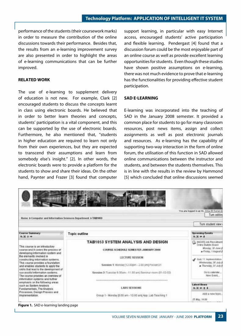
E-learning was incorporated into the teaching of SAD in the January 2008 semester. It provided a common place for students to go for many classroom resources, post news items, assign and collect assignments as well as post electronic journals and resources. As e-learning has the capability of supporting two-way interaction in the form of online forum, the utilisation of this function in SAD allowed online communications between the instructor and students, and between the students themselves. This is in line with the results in the review by Hammond [5] which concluded that online discussions seemed
Figure 1. SAD e-learning landing page

24 PLATFORM VOLUME SEVEN NUMBER ONE JANUARY - JUNE 2009
Technology Platform: APPLICATION OF INTELLIGENT IT SYSTEM
to offer most to collaboratively minded learners comfortable with ICT and studying a topic requiring conceptual understanding. Hence, discussion room could be best used to support teaching and learning as the SAD course is very conceptual in nature. Figure 1 shows the SAD e-learning landing page.
Besides the instructor, the students were also allowed to start their own discussion topic in the forum. This enabled them to discuss their topic of interest as well as share their questions, the answers that were replied, their opinions and ideas. Thus, e-learning discussion room was able to support asynchronous forums with the standard capabilities to post a new message, reply to a message and follow available threads. In order to create the discussion room, the instructor provided the directions, access permission (read, reply, post) and grading options for participation. The instructor also participated in the discussion forum by replying to their queries.
For this study, the students’ data log of activity of the e-learning system were captured at the end of the semester. The data were used in analysing the students’ access rates of the discussion forum which indicated their active participation. In order to estimate the degree of relationship between frequency of access of the discussion room and students’ performance, the Spearman correlation coefficients were calculated by using the students’ coursework marks and the frequency of access. Further analysis was also made on the discussion rooms to identify the topics initiated and types of topics. In order to improve e-learning in the SAD course, a small survey in the form of a questionnaire, which contained 11 questions, were conducted during the study week of the semester. 38 students from the SAD class responded to the survey.
RESULTS AND DISCUSSIONS
Frequency of student access
Figure 2 shows the compilation of statistics on access of the discussion room throughout the semester. Due to the huge diversity in terms of the number of access
for each student, in the figure, these numbers are presented in ranges in steps of 25 accesses.
From Figure 2, it can be seen that around 37.6% of the students accessed the discussion room for less than 50 times throughout the semester. Another 18.8% of the students found it to be very interesting to be actively involved in the discussion room. This group of students accessed the discussion room more than 175 times. The rest, who made up the other 43.6% of the students, accessed the room between 50 to 175 times in the whole semester.
Access frequency vs performance
In order to estimate the degree of relationship between frequency of access of the discussion room and students’ performance, the Spearman correlation coefficients ρ were calculated using the data for the chosen groups of students. A correlation coefficient indicates the degree of relationship between two sets of data. If there is no correlation, the correlation coefficient is 0.00. If the correlation is perfect, the value is equal to 1.00. The data was analysed using SPSS and the coefficients ρ obtained was 0.000. This shows that there is no significant relation between the frequency of access and student performance. As pointed out by Hammond [4], this could be because the students were free to contribute as and when they liked and the topics for the discussion were loosely guided by the lecturer.
46
40
2320 21
1216
3
48
05
101520253035404550
no
. o
f st
ud
ents
0-25
26-5
0
51-7
5
76-1
00
100-
125
126-
150
151-
175
176-
200
>201
access range
Figure 2. Frequency of student access
25 VOLUME SEVEN NUMBER ONE JANUARY - JUNE 2009 PLATFORM
Technology Platform: APPLICATION OF INTELLIGENT IT SYSTEM
Analysis on topics of discussion
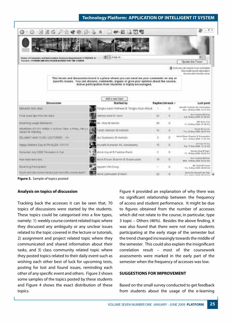
Tracking back the accesses it can be seen that, 70 topics of discussions were started by the students. These topics could be categorised into a few types, namely: 1) weekly course content related topic where they discussed any ambiguity or any unclear issues related to the topic covered in the lecture or tutorials, 2) assignment and project related topic where they communicated and shared information about their tasks, and 3) class community related topic where they posted topics related to their daily event such as wishing each other best of luck for upcoming tests, posting for lost and found issues, reminding each other of any specific event and others. Figure 3 shows some samples of the topics posted by these students and Figure 4 shows the exact distribution of these topics.
Figure 4 provided an explanation of why there was no significant relationship between the frequency of access and student performance. It might be due to figures obtained from the number of accesses which did not relate to the course, in particular, type 3 topic – Others (46%). Besides the above finding, it was also found that there were not many students participating at the early stage of the semester but the trend changed increasingly towards the middle of the semester. This could also explain the insignificant correlation result – most of the coursework assessments were marked in the early part of the semester when the frequency of accesses was low.
SUGGESTIONS FOR IMPROVEMENT
Based on the small survey conducted to get feedback from students about the usage of the e-learning
Figure 3. Sample of topics posted

26 PLATFORM VOLUME SEVEN NUMBER ONE JANUARY - JUNE 2009
Technology Platform: APPLICATION OF INTELLIGENT IT SYSTEM
facility, the majority of the students declared they accessed it more than 5 times each week. The result is shown in Figure 5.
The component of the e-learning most often accessed (63%) was the lecture notes. Discussion room was the second (26%). Figure 6 shows the results.
The most useful component of the e-learning was again the lecture notes and the discussion room came second. Figure 7 presents the breakdown of the students’ preferences.
From these three feedback results, it was found that students used e-learning frequently and the use of e-learning for uploading lecture notes and course materials were deemed useful to them. The discussion room was also found to be useful to them in sharing their ideas, concerns and thoughts. Feedback from students also highlighted the instructor’s active participation, in that the immediate response in the discussion encouraged them to participate effectively and made the discussion livelier. Some of them commented that, the online discussions allowed students to share knowledge and information, to update and discuss related matters with lecturers and friends. Thus, future e-learning modules planned for the course should take these results into consideration in order to provide a more effective online learning environment.
CONCLUSION AND FUTURE WORK
In conclusion, the discussion room of the e-learning module was able to provide the platform for a student’s active participation. It attracted a considerable number of students to participate actively. However, the topics discussed among the students needed to be monitored in order to have an impact on the students’ performance. As 46% of the topics discussed were non-course related, there was no correlation between the frequency of participation and performance. However, the results from a survey suggested that the discussion room was useful to the students. Hence, this suggests that the discussion room should be incorporated in future
Figure 4. Distribution of topics posted
Weekly course 32%
Assignment 22%
Others46%
0
10
20
30
40
50
60
70
80
never once depends 2-4 > 5
no. o
f stu
dent
s
access frequency
Figure 5. Number of accesses per week
Figure 6. Most accessed components
Figure 7. Most useful components
discussion room26%
announcements8%
online quizzes3%
lecture notes63%
discussion room26%
announcements16%
online quizzes5%
lecture notes53%

27 VOLUME SEVEN NUMBER ONE JANUARY - JUNE 2009 PLATFORM
Technology Platform: APPLICATION OF INTELLIGENT IT SYSTEM
plans for e-learning of courses. With proper control of the discussion room, it is believed that the point stated by Johnson [6] where the online learning environment had a greater impact on students learning than teaching styles, classroom environment and educational impact, can be realised.
For future work, this study suggests a more thorough survey on a larger number of participants for the collection of feedback on the usage of e-learning in the teaching and learning process.
REFERENCES
[1] Dennis, A. Wixom, B. H. and Tegarden, D. Systems Analysis and Design with UML Version 2.0 An Object-Oriented Approach, 2nd Edition, USA: John Wiley and Sons, Inc. 2005.
[2] Martyn Clark, Getting Participation Through discussion, ACM SIGCSE Bulletin, March 2000 Vol 32. No 1. pp 129-133.
[3] Paynter, J. Ong, J and Frazer, L. 2000. A Preliminary Comparison of Computer Mediated Training Tools. Proceedings of the 7th Asia Pacific Software Engineering Conference (APSEC2000). pp. 402-406.
[4] Pendergast, M. (2006). An Analysis Tool for the Assessment of Student Participation and Implementation Dynamics in Online Discussion Forums. ACM SIGITE Newsletter, Volume 3. No. 2. pp. 10-17.
[5] Hammomd, M. (2005). A Review of Recent Papers on Online Discussion in Teaching and Learning in Higher Education. Journal of Asynchronous Learning Networks. Volume 9. No 3. pp. 9-23.
[6] Johnson, C.M. (2001). A Survey on Current Research on Online Communities Practice, Internet an Higher Education, Vol 4, pp45-60.
Aliza Sarlan received her first degree (Information Technology) from Universiti Utara Malaysia in 1996, her Masters degree (Information Technology) from University of Queensland, Australia in 2002. She is currently lecturing at the Computer & Information Sciences Department Universiti Teknologi PETRONAS. Her research interests are in Information
System Management and Application Development in Organisational Context. Currently, her research focuses on the interdependencies of information technologies and organisational structure, IS policy and strategic implementation of ICT in healthcare industry.
Dr Wan Fatimah Wan Ahmad received her BA and MA degrees in Mathematics from California State University, Long Beach, California USA in 1985 and 1987. She also obtained Dip. Ed. from Universiti Sains Malaysia in 1992. She completed her PhD in Information System from Universiti Kebangsaan Malaysia in 2004. She is currently a senior lecturer at Computer &
Information Sciences Department of Universiti Teknologi PETRONAS, Malaysia. She was a lecturer at Universiti Sains Malaysia , Tronoh before joining UTP. Her main interests are in the areas of mathematics education, educational technology, human computer interaction and multimedia. She can be reached at [email protected].

28 PLATFORM VOLUME SEVEN NUMBER ONE JANUARY - JUNE 2009
Technology Platform: APPLICATION OF INTELLIGENT IT SYSTEM
INTRODUCTION
According to Moon, C. et al. [1], performance appraisal of candidates in relation to a particular position is a key task towards managing the human resource of an organisation. Supervisors are concerned with performance appraisal judgments and evaluations that they have to make on their subordinates. On the other hand, subordinates are increasingly realising the importance of performance appraisal since it would very much affect their rewards and future career path. As the world began to shift towards knowledge-based capitalism, all organisations are reminded of the importance of maintaining their talented knowledge workers [1]. Therefore, discovering and promoting the most qualified candidates is essential because valuable human expertise is the main source of competitive advantage for the organisations. Thus, the creation of a performance criteria is an important requirement towards performance appraisal [2].
A performance appraisal is usually conducted periodically within an organisation to examine and discuss the work performance of subordinates so as to identify the strengths and weaknesses as well as opportunities for improvement among employees. Following this, most employers use performance appraisal results to determine if a particular staff should be terminated or reinforced; as an employee development and coaching tool; to give a practical evaluation of an employee’s readiness for promotion; and to serve as the foundation for giving merit bonus.
Following the awareness and understanding of the concept of fuzzy sets, some researchers have applied the fuzzy sets theory to the performance appraisal process. However, Khairul, A. R and Qiang, S. [3] mentioned that, there is an argument regarding one of the most suitable ways of managing multiple variables of imprecise data to apply fuzzy concept reasoning which reflects the way of human-thinking.
PERFORMANCE APPRAISAL SYSTEM USING MULTIFACTORIAL EVALUATION MODEL
C.C. Yee, Chen Yoke Yie*Universiti Teknologi PETRONAS, 31750 Tronoh, Perak Darul Ridzuan, Malaysia
ABSTRACT
Performance appraisal of employees is important in managing the human resource of an organisation. With the change towards knowledge-based capitalism, maintaining talented knowledge workers is critical. However, management classification of “outstanding”, “poor” and “average” performances may not be an easy decision. Besides that, superiors might also tend to judge the work performance of their subordinates informally and arbitrarily especially without the existence of a system of appraisal. The proposal in this paper is a performance appraisal system using multifactorial evaluation model in dealing with appraisal grades which are often expressed vaguely in linguistic terms. The proposed model is for evaluating staff performance based on a specific performance appraisal criteria. The project was a collaboration with one of the Information and Communication Technology companies in Malaysia with reference to its performance appraisal process.
Keywords: Multifactorial Evaluation Model, performance appraisal system, decision support system, fuzzy sets
This paper was presented at the 2009 International Conference on Computer and Information Technology, Japan 27 - 29 May 2009
29 VOLUME SEVEN NUMBER ONE JANUARY - JUNE 2009 PLATFORM
Technology Platform: APPLICATION OF INTELLIGENT IT SYSTEM
Various studies were conducted to improve the application of fuzzy sets theory and fuzzy logic in areas of performance appraisals. This paper aimed to develop a performance appraisal system by applying the fuzzy set theory in dealing with appraisal grades often expressed vaguely in linguistic terms. The proposal was to use multifactorial evaluation model, an application of fuzzy set theory to the decision making process, in the performance appraisal system.
RELATED WORK
Performance Appraisal System
Performance appraisal is a formal management system that provides for the evaluation of the quality of an individual’s performance in an organisation [4]. As mentioned by Dessler, G [5], performance appraisal has the means to evaluate an employee’s current and past performance relative to the employee’s performance standards. It is a process which involves creating work standards; evaluating employee’s actual performance relative to those work standards; and giving feedback to the employee so as to motivate him or her to improve on job performance or to eliminate performance deficiencies. In addition, Terrence, H. M. and Joyce, M. [6] stated that, some potential aims of a performance appraisal might include identifying a particular behaviour or job.
Various techniques or methods have been used by human resource management experts to evaluate the performance of an employee. As outlined by Vicky G. [7], some of the appraisal methods included ranking; trait scales, critical incidents, narrative and criteria-based. Terrence, H. M. and Joyce, M. [6] mentioned a few other methods including management-by-objectives (MBO), work planning and review, 360° appraisal and peer review. With all these available techniques, it is essential to understand that different organisations might use different techniques in assessing staff performances. Since all these techniques mentioned have their own advantages and disadvantages, most organisations mix and match different techniques for their own performance appraisal system to fulfill their organisational needs.
The performance appraisal system has become one of the most valuable management tools in which organisation members use to achieve collective goals. In order to ensure that the results of the performance appraisals are useful and reasonable to the superior when evaluating their subordinates, it is important that the performance appraisal system consistently produce reliable and valid results for the management of an organisation.
Application of Fuzzy Based Method
The fuzzy based method has been applied into several performance appraisal systems. Moon, C. et al. [1] proposed a methodology utilising fuzzy set theory and electronic nominal group technology for multi-criteria assessments in the group decision-making of promotion screening. The study suggested that the methodology is a good method for a transparent and fair multi-criteria performance evaluation in military organisations.
Researchers have demonstrated that the fuzzy set theory could be successfully used to solve multiple criteria problems [8]. This is because, in many circumstances, the appraiser tended to use vaguely defined qualitative criteria in evaluating the performance of their subordinates. This created difficulties for the appraiser to precisely quantifying the score of each candidate. Jing. R.C et al. [8] worked on applying fuzzy set theory on computer-based fuzzy group decision support system (FGDSS). Based on the findings of their work, the application of fuzzy set theory in FGDSS is said to be able to assist the decision maker in making better decisions under different circumstances and alternatives [1].
A good example of the application of the fuzzy-set theory to decision-making process is the multifactorial evaluation model [9]. For example, Tutmez et al. [10] used a multifactorial fuzzy approach to evaluate the sawability and selected a suitable diamond saw for a new building stone. This study suggested that information can be reasonably obtained and sawability classification is reasonable and acceptable.
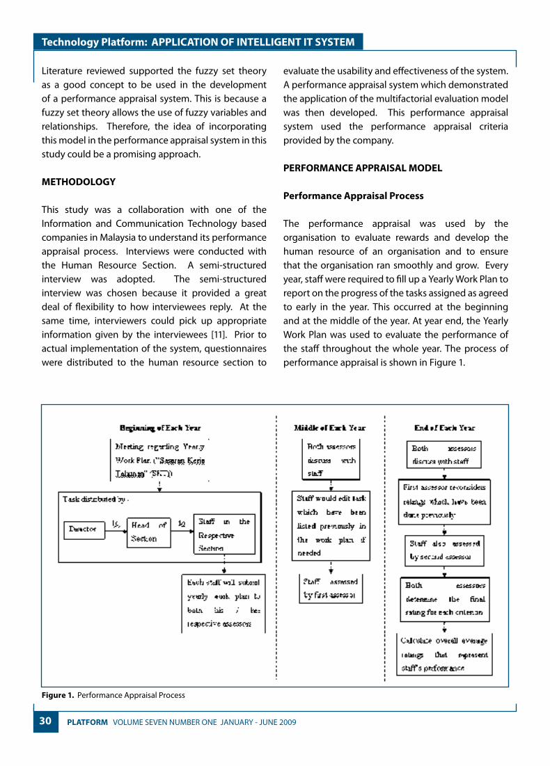
30 PLATFORM VOLUME SEVEN NUMBER ONE JANUARY - JUNE 2009
Technology Platform: APPLICATION OF INTELLIGENT IT SYSTEM
Literature reviewed supported the fuzzy set theory as a good concept to be used in the development of a performance appraisal system. This is because a fuzzy set theory allows the use of fuzzy variables and relationships. Therefore, the idea of incorporating this model in the performance appraisal system in this study could be a promising approach.
METHODOLOGY
This study was a collaboration with one of the Information and Communication Technology based companies in Malaysia to understand its performance appraisal process. Interviews were conducted with the Human Resource Section. A semi-structured interview was adopted. The semi-structured interview was chosen because it provided a great deal of flexibility to how interviewees reply. At the same time, interviewers could pick up appropriate information given by the interviewees [11]. Prior to actual implementation of the system, questionnaires were distributed to the human resource section to
evaluate the usability and effectiveness of the system. A performance appraisal system which demonstrated the application of the multifactorial evaluation model was then developed. This performance appraisal system used the performance appraisal criteria provided by the company.
PERFORMANCE APPRAISAL MODEL
Performance Appraisal Process
The performance appraisal was used by the organisation to evaluate rewards and develop the human resource of an organisation and to ensure that the organisation ran smoothly and grow. Every year, staff were required to fill up a Yearly Work Plan to report on the progress of the tasks assigned as agreed to early in the year. This occurred at the beginning and at the middle of the year. At year end, the Yearly Work Plan was used to evaluate the performance of the staff throughout the whole year. The process of performance appraisal is shown in Figure 1.
Figure 1. Performance Appraisal Process

31 VOLUME SEVEN NUMBER ONE JANUARY - JUNE 2009 PLATFORM
Technology Platform: APPLICATION OF INTELLIGENT IT SYSTEM
Figure 2. Proposed Application of Multifactorial Evaluation Model in Performance Appraisal System
Staff Evaluation
Four aspects were taken into consideration when evaluating staff performance and each aspect was indexed into its sub-criterion, as follows:
(a) Working output (Aspect 1): This aspect evaluates the quantity, quality and effectiveness of the staff’s working output and punctuality.
(b) Knowledge and skills (Aspect 2): This aspect evaluates the staff’s knowledge and skills in the working field, their effectiveness in communications and realisation of rules.
(c) Personal quality (Aspect 3): This aspect evaluates the personal quality appreciated by the organisation such as discipline, proactive, innovative, cooperativeness and independence.
(d) Informal Event(s) and Contribution(s) (Aspect 4): Staff’s contribution to the organisation, community, state, country and international.
When evaluating staff’s performance, the appraiser would use a scale of 1 to 10 to rate each sub-criterion for each aspect mentioned above. 1 indicates that the staff was rated poorly in that particular sub-criterion and 10 indicates that the staff was rated highly. The verbal grade for the scale is shown in Table 1:
Table 1. Verbal Grades And Scale For Each Aspect
Verbal Grades ScaleVery High 9 Or 10
High 7 Or 8Moderate 5 Or 6
Low 3 Or 4Very Low 1 Or 2

32 PLATFORM VOLUME SEVEN NUMBER ONE JANUARY - JUNE 2009
Technology Platform: APPLICATION OF INTELLIGENT IT SYSTEM
PERFORMANCE APPRAISAL SYSTEM
The proposed application of Muiltifactorial Evaluation Model in the performance appraisal system is a combination of four multifactorial evaluation models.
As shown in Figure 2, each of the models represented an aspect to be evaluated in the performance appraisal. After getting the staff’s performance on each aspect from their superior, the staff’s overall average ratings was calculated by following the equation shown in Figure 2. U represents the factors to be evaluated in each aspect whereas D(u) is the result of the staff’s performance in a particular aspect.
The first evaluation model in Figure 2 used U1, that is, the factors in Aspect 1 (Working Output) as its input. The sub-criterion for this aspect was used as the basic factor under this aspect which are: f1 = Quantity of Working Output, f2 = Quality of Working Output, f3 = Punctuality, and f4 = Effectiveness of Working Output.Therefore, F = {f1, f2, f3, f4}.
The verbal grades used for the appraisal are: e1 = Very High, e2 = High, e3 = Moderate, e4 = Low, and e5 = Very LowTherefore, E = {e1, e2, e3, e4, e5}.
For a staff’s performance in terms of working output, the single-factor evaluation for each aspect was determined by the executives in the Administration Section of the company. As an example, the weightage of the “Quantity of Working Output” factor f1 were, 10% for Very High, 40% for High, 30% for Moderate, 10% for Low, and 10% for Very Low. Thus, the single-factor evaluation vector R1(u) is: R1(u) = {0.1, 0.4, 0.3, 0.1, 0.1}
In the same way, the single-factor evaluation vectors for f2, f3, and f4 were obtained as below:-
R2(u) = {0.2, 0.5, 0.2, 0.1, 0.0} R3(u) = {0.5, 0.3, 0.1, 0.1, 0.0} R4(u) = {0.2, 0.5, 0.2, 0.1, 0.0}
As a result, by referring to these single-factor evaluation vectors, the following evaluation matrix was built:-
R(u) =
R1(u)
=
0.1 0.4 0.3 0.1 0.1
R2(u) 0.2 0.5 0.2 0.1 0.0
R3(u) 0.5 0.3 0.1 0.1 0.0
R4(u) 0.2 0.5 0.2 0.1 0.0
W(u) are the weighting factors. Therefore, it is the appraiser’s rating towards a staff for the sub-criterion of a particular aspect. As an example, assume that the appraiser’s rating for the weight vector which corresponding to the four factors in all aspects are:
W1(u) = {0.2, 0.3, 0.3, 0.2} W2(u) = {0.3, 0.4, 0.3} W3(u) = {0.2, 0.3, 0.2, 0.3} W4(u) = {0.1}
Multiplication of matrices W(u) and R(u) were based on the min-max composition of fuzzy relations, where the resulting evaluation was in the form of a fuzzy set D(u) = [d1, d2, d3, d4] [9]. Since the aspect of Working Output were of five verbal grades, that is, E = {e1, e2, e3, e4, e5} involved in the performance appraisal system, thus, the resulting evaluation in the form of a fuzzy set D(u) = [d1, d2, d3, d4, d5] is:
D(u) = W1(u) . R(u)
= [0.2 0.3 0.3 0.2] .
0.1 0.4 0.3 0.1 0.1
0.2 0.5 0.2 0.1 0.0
0.5 0.3 0.1 0.1 0.0
0.2 0.5 0.2 0.1 0.0
= [0.3 0.3 0.2 0.1 0.1]
They were calculated through the following steps whereby ^ represent the operations min and v represent the operation max.

33 VOLUME SEVEN NUMBER ONE JANUARY - JUNE 2009 PLATFORM
Technology Platform: APPLICATION OF INTELLIGENT IT SYSTEM
d1 = (w1 ^ r11) v (w2 ^ r21) v (w3 ^ r31) v (w4 ^ r41) = (0.2 ^ 0.1) v (0.3 ^ 0.2) v (0.3 ^ 0.5) v (0.2 ^ 0.2) = 0.1 v 0.2 v 0.3 v 0.2 = 0.3 d2 = (w1 ^ r12) v (w2 ^ r22) v (w3 ^ r32) v (w4 ^ r42) = (0.2 ^ 0.4) v (0.3 ^ 0.5) v (0.3 ^ 0.3) v (0.2 ^ 0.5) = 0.2 v 0.3 v 0.3 v 0.2 = 0.3 d3 = (w1 ^ r13) v (w2 ^ r23) v (w3 ^ r33) v (w4 ^ r43) = (0.2 ^ 0.3) v (0.3 ^ 0.2) v (0.3 ^ 0.1) v (0.2 ^ 0.2) = 0.2 v 0.2 v 0.1 v 0.2 = 0.2 d4 = (w1 ^ r14) v (w2 ^ r24) v (w3 ^ r34) v (w4 ^ r44) = (0.2 ^ 0.1) v (0.3 ^ 0.1) v (0.3 ^ 0.1) v (0.2 ^ 0.1) = 0.1 v 0.1 v 0.1 v 0.1 = 0.1 d5 = (w1 ^ r15) v (w2 ^ r25) v (w3 ^ r35) v (w4 ^ r45) = (0.2 ^ 0.1) v (0.3 ^ 0.0) v (0.3 ^ 0.0) v (0.2 ^ 0.0) = 0.1 v 0.0 v 0.0 v 0.0 = 0.1
The largest components of D(u) were d1 = 0.3, and d2 = 0.3 at the same time. Referring to the verbal
grades, E = {Very High, High, Moderate, Low, very Low}, the analysed staff’s performance in terms of working output obtained a rating somewhere between “Very High” and “High”. However, by applying the principle of the biggest subjection degree as mentioned by Guifeng, G. et al. [12], the staff’s performance in terms of working output is “Very High”.
The same method of calculation was applied to U2, U3, and U4, that is, the aspect of Knowledge and Skills, the aspect of Personal Quality, and the aspect of Informal Event(s) and Contribution(s), respectively. Following this, the verbal grades and weighting for each aspect as shown in Table 2 were referred when calculating a staff’s overall average rating.
The staff’s overall average rating (AR) is: AR = (Aspect 1 * 50) + (Aspect 2 * 25) + (Aspect 3 * 20) + (Aspect 4 * 5)
Based on Table 2, the analysed staff’s performance in terms of working output obtained a rating of “Very High”. As a result, 1.0 would be the weighting for Aspect 1. Computation using the multifactorial evaluation model rated the staff as “Moderate” or a weighting of 0.6 in terms of Knowledge and Skill. For the aspect of Personal Quality, the staff’s performance was “Excellent” or a weighting of 1.0. For Informal Event(s) and Contribution(s), the staff gained an “Active” performance or a weighting of 0.8. The rating and weighting for each aspect is summarised in Table 3.
Therefore, the staff’s overall average rating (AR) is: AR = (1.0 * 50) + (0.6 * 25) + (1.0 * 20) + (0.8 * 5) = 89
Table 2. Verbal Grades And Weighting For Each Aspect
Aspect Verbal Grades Weighting for Each Aspect
Aspect 1
Very High 1.0High 0.8
Moderate 0.6Low 0.4
Very Low 0.2
Aspect 2
and 3
Excellent 1.0Good 0.8
Moderate 0.6Weak 0.4
Very Weak 0.2
Aspect 4
Very Active 1.0Active 0.8
Moderately Active 0.6
Less Active 0.4Not Active 0.2
Table 3. Summarised Rating And Weightage Of The 4 Aspects
Aspect Rating WeightingAspect 1 Very High 1.0Aspect 2 Moderate 0.6Aspect 3 Excellent 1.0Aspect 4 Active 0.8

34 PLATFORM VOLUME SEVEN NUMBER ONE JANUARY - JUNE 2009
Technology Platform: APPLICATION OF INTELLIGENT IT SYSTEM
As a result, according to this calculation of the AR and by referring to Table 4, the staff would be categorised in the “High Performer(s)” group.
CONCLUSION
This study presented an illustrative example of the application of one of the fuzzy set theory in a multi-criteria performance appraisal system. A performance appraisal system was developed utilising the performance appraisal criteria from an Information and Communication Technology based company in Malaysia. This system used a multifactorial evaluation model to assist high-level management, particularly in the case study, to appraise employees. The concept of using four multifactorial evaluation models in the performance appraisal system eased the changes that needed to be made to the system whenever necessary. This model followed a systematic step in determining a staff’s performance, thereby, creating a system of appraisal which was able to consistently produce reliable and valid results in the appraisal process. In order for this system to be applied in other companies, the aspect to be evaluated and the
weightage for each of these aspects needed to be defined beforehand.
REFERENCES
[1] Moon, C., Lee, J., Jeong, C., Lee, J., Park, S. and Lim, S. (2007), “An Implementation Case for the Performance Appraisal and Promotion Ranking”, in IEEE International Conference on System, Man and Cybernetics, 2007.
[2] Adnan, S. and Minwir, A. (1998), “Fuzzy Logic Modeling for Performance Appraisal Systems – A Framework for Empirical Evaluation”, Expert Systems with Applications, Vol. 14, No. 3, p. 323-328.
[3] Khairul, A. R and Qiang, S. (2006), “Data-Driven Fuzzy Rule Generation and Its Application for Student Academic Performance Evaluation”, Applied Intelligence, Vol. 25, Issue. 3. p. 305-319.
[4] Ab. Aziz Yusof. (2003), Performance Appraisal Issues, Challenges & Prospects, Pearson.
[5] Dessler, G. (2000), Human Resource Management (8th Edition), New Jersey, Pearson Education, Inc.
[6] Terrence, H. M. and Joyce, M. (2004), Performance Appraisals, ABA Labor and Employment Law Section, Equal Employment Opportunity Committee.
[7] Vicky, G. (2002), Performance Appraisals, Loss Control Services, Texas Association of Counties.
[8] Jing, R.C, Cheng, C. H. and Chen, L. S. (2007), “A Fuzzy-Based Military Officer Performance Appraisal System”, Applied Soft Computing, Vol. 7, Issue. 3, p. 936-945.
[9] Mehmed, K. (2003), Data Mining Concepts, Models, Methods, and Algorithms, Wiley-Interscience.
[10] Tutmez, B., Kahraman, S. and Gunaydin, O. (2006), “Multifactorial Fuzzy Approach to the Sawability Classification of Building Stones”, Construction and Building Materials, Vol. 21, Issue 8, p. 1672-1679.
[11] Emma, B. and Bryman, A. (2003), Business Research Methods. US: Oxford University Press.
[12] Guifeng, G., Luo, Y. and Yan, B. (2006), “Fuzzy Evaluation System of Traffic Safety in Highway Tunnel” http://lib.hpu.edu.cn/comp_meeting/progress%20in%20safety%20science%20and%20technology%20vol.v1/1989.doc [Accessed on 23th December 2008]
Chen Yoke Yie obtained her MSc degree in Business Information Technology from University of Manchester, UK in 2007. She is currently lecturing at the Department of Computer and Information Sciences, University of Technology PETRONAS, Malaysia. Her field of interest includes Intelligent System, Text Mining and E-Business.
Table 4. Benchmark/Standard Used In Determining Staff’s Performance
Overall Average Ratings
Group Remarks
Above 80% High Performer(s)
• Entitled for “Best Service Award”.
• An incentive of RM 1000.
• A certificate of appreciation.
Less than 80% but more than 50%
Average Performer(s)
• Advised to improve their performance in the coming year.
Less than 50%
Low Performer(s)
• Disciplinary action might be taken towards the staff.
• Should constantly report his / her work progress to his / her assessors in a stated period.

35 VOLUME SEVEN NUMBER ONE JANUARY - JUNE 2009 PLATFORM
Technology Platform: APPLICATION OF INTELLIGENT IT SYSTEM
INTRODUCTION
The birth of knowledge management was from recognising the complexities in finding the right information or knowledge, and the complexities in achieving the demands of the current dynamic nature of business. As businesses nowadays shift focus from an industrial-based to a service-based economy, there is an urge for the organisation to leverage on existing knowledge to be ahead of their competitors. Most organisations are aware of the value and contribution of knowledge towards sustaining business goals and will take steps to implement the systems or applications that fit into their business goals.
The idea to implement the Expert Directory System (EDS) at a unit which manages the E&P Business for a multinational oil and gas corporation was initiated when the organisation was fraught with high employee turnover and difficulty in sustaining their knowledge workers. As experienced employees
left the organisation, they took away knowledge they possessed. This knowledge used to be part of the organisation’s assets, as the employees in any knowledge-based organisation are. In the highly competitive oil and gas industry, such knowledge and experience are highly valued and the loss will impact on the organisation’s bottom line.
Thus, the implementation of the Expert Directory System (EDS) is critical to capture, organise, distribute, share and store the knowledge for reuse when needed. The Expert Directory System (EDS) running on the web platform is meant to efficiently distribute knowledge that exists in the organisation to the people who need it.
The current practice to use emails as the medium for discussion is not proper as old emails will be deleted at specific times for housekeeping as well as it is hard to search when the knowledge is needed. The EDS would allow knowledge workers in the organisation
This paper was presented at the 4th International Conference on Information Technology and Multimedia
at UNITEN (ICIMU’ 2008), Malaysia, 17 – 19 November 2008
USING ONTOLOGY FOR THE DEVELOPMENT OF A KNOWLEDGE-BASED SYSTEM FOR E&P BUSINESS
Ainol R. Shazi*, Mazeyanti M Ariffin, Fatihah KasimUniversiti Teknologi PETRONAS, 31750 Tronoh, Perak Darul Ridzuan, Malaysia
ABSTRACT
This paper discusses the development of a knowledge-based system (KBS) for the exploration and production (E&P) business based on a domain specific ontology. The E&P is one that is fraught with high employee turnover due to volatile market trends. The introduction of a KBS to capture the knowledge of industry experts will aid the preservation of knowledge assets within the organisation. In order to ensure the comprehensiveness of the captured knowledge and that the knowledge is interpreted within the correct context, an ontology was developed prior to the development of the KBS. The KBS, called the Expert Directory System (EDS), was then developed based on the ontology and this paper includes a discussion on the EDS implementation.
Keywords: ontology, knowledge-based, exploration and production
36 PLATFORM VOLUME SEVEN NUMBER ONE JANUARY - JUNE 2009
Technology Platform: APPLICATION OF INTELLIGENT IT SYSTEM
to share best practices and lessons learnt among team projects and colleagues, discussions on current projects as well as sharing of ideas and suggestions. The knowledge domain for the development of the EDS was first modeled using a knowledge map which was then converted into an ontology before building the system.
As the Expert Directory System (EDS) was intended to be used in the oil and gas industry, the development of the ontology could help to create a common understanding of the information structure among people or software agents [12]. Thus, it is proposed that the ontology be used to structure the knowledge base system so that it can be re-used for a variety of applications [15].
LITERATURE REVIEW
Nonaka [11] defined knowledge management as justified true skill, a dynamic human process of justifying personal belief and skill towards the truth. Leonard-Barton [7,8] stressed the importance of knowledge with successful innovations with views of activities in an organisation. Knowledge management became part of visualising and cultivating knowledge and ways to leverage on other people’s expertise as well as organisation’s intangible intellectual assets for more value.
With knowledge management, organisations could create and utilise the best possible capital hidden in peoples' minds through tools for measuring intangible assets. According to Boisot [4], knowledge management in his view is to manage knowledge assets as a social learning process. Capabilities, technology and competence are the representations of the knowledge assets operating in different levels of an organisation but it is specialised interpersonal social relationship that reinforces the importance of the assets.
To manage knowledge efficiently, an organisation needs to have a highly flexible and adaptable organisational structure. Pralahad and Hamel [13] suggested that in the present environment,
organisations should be structured on the basis of core competencies because these structures can sustain a high level of environmental uncertainty and chaos. Thus, generally with these theories, knowledge management is a process of facilitating knowledge-related activities, such as creation, capture, transformation and use of knowledge [2]. To integrate diverse sets of tasks and implementation of powerful information systems, such as Internet and intranets, the management processes will include a range of activities ranging from learning, collaboration and experimentation.
Knowledge sharing is important and critical for organisations which are large and geographically scattered in different locations [3]. By sharing knowledge, members of an organisation can increase their knowledge and thus create “organisational knowledge”. Knowledge that is internalised within the organisation is not produced by organisational members alone, but created through interactions amongst them [5].
Individual knowledge, if not shared with others, will have very little effect on the organisational knowledge base. One of the most important tasks for management is to facilitate the process of interactions between employees and make them sensitive towards environmental stimuli so that their individual knowledge is internalised to contribute to the organisational knowledge base [10].
There are three major forces that could be combined to attract organisations to implement knowledge management [14]: the increase of knowledge dominance as a basis of organisational effectiveness, failure of financial models to represent the dynamics of knowledge and the failure of information technology which stands alone. The failure of information technology can happen when an organisation fail to rationalise the needs of the organisation in terms of users of the technology and the failure to combine it with the knowledge management concept itself. Sharp [14] found that the combination of at least two of the following factors has resulted in the successful implementation of

37 VOLUME SEVEN NUMBER ONE JANUARY - JUNE 2009 PLATFORM
Technology Platform: APPLICATION OF INTELLIGENT IT SYSTEM
knowledge management solutions: communication within the organisation, collaboration and teamwork, commitment by employees to the practice of KM, innovative corporate culture and the application of appropriate technology.
Methodologies, techniques and tools are central to a process and information system and to process development. Comprehensive methodologies using step-by-step approaches guide the development of a system or process. Techniques are specific processes used in conjunction with one or more methodologies that result in comprehensive deliverables. Tools are computer programs that facilitate the implementation of techniques within the overall guidelines of any particular development methodology [9].
The ontology and its associated paradigm often used in the knowledge representation for knowledge-based or knowledge management systems is adopted from philosophy. As such, the exact definition of ontology and the ‘correct’ representation of knowledge in ontologies is highly debated. In general, an ontology is a formal explicit description of concepts (sometimes called classes) in a domain of discourse, properties of each concept describing various features and attributes of the concept, and restrictions on slots (sometimes called roles or properties). An ontology together with a set of individual instances of classes constitutes a knowledge base [12]. However, not everyone adopts the ontology for knowledge representation; there are also some [1] who prefer to use concept maps for knowledge representation. At the same time, it is important to take into consideration the context of the domain before interpreting a particular ontology.
Due to the varying interpretations of ontology in the sphere on information systems (IS), this paper will adopt one definition that is most suited to reflect the purpose of the project. Zuniga [16] elaborated on two prominent views of ontology in information systems and defined an IS ontology as follows:
“An IS ontology is an axiomatic theory made explicit by means of a specific formal language. The IS ontology is designed for at least one specific and practical
application. Consequently, it depicts the structure of a specific domain of objects, and it accounts for the intended meaning of a formal vocabulary or protocols that are employed by the agents of the domain under investigation.”
Thus, it becomes clear that ontologies developed for IS purposes must be functional, and takes into consideration the constraints and restrictions of the particular domain. In the area of exploration and production (E&P) within the oil and gas industry, the usage of ontology-driven systems development is rather limited.
This study used ontology as the guide for the system design and development because it supports greater efficiency and adaptability of the resulting software. Noy and McGuinness [12] list the following as reasons why people use ontologies:• Sharing of common understanding on structure
of information among people or software agents• Reuse of domain knowledge• Making domain assumptions explicit• Separation of domain knowledge from operational
knowledge• To analyse domain knowledge
METHODOLOGY
According to Gruber [6], an ontology is an explicit specification of the terms in the domain and relations among them and is an alternative way to represent the knowledge in the domain. The main purpose of developing an ontology is to create a common understanding of the terms and the structure of information among people and software which then leads to reuse of knowledge in the domain [12].
In designing the ontology for the EDS, this study adopted the basic methodologies described by Uschold and Gruniger [15]. The first step was to identify the purpose of developing the ontology. In this case, the ontology was developed for the usage of the people in the E&P business area.

38 PLATFORM VOLUME SEVEN NUMBER ONE JANUARY - JUNE 2009
Technology Platform: APPLICATION OF INTELLIGENT IT SYSTEM
A session was conducted to identify the existing knowledge that needed to be leveraged in the organisation. The resulting ontology represented the relationships between the knowledge objects which was later used as the basis of the EDS implementation.
This study also adopted the iterative and incremental development methodology for developing the EDS. The basic idea behind iterative enhancement was to develop a software system incrementally, allowing what was learned during earlier development for later incremental, deliverable versions of the system – where possible, learning would come from both the development and use of the system. Key steps in the process were to start with a simple implementation of a subset of the software requirements and iteratively enhance the evolving sequence of versions until the full system is implemented.
Use-Case Development
A use case as in Figure 1 was constructed to represent the distinct business functionality in a system. In the Expert Directory System, the normal user could perform the functions: add data, edit data, delete data, search data, upload file and perform discussions with colleagues or experts. Administrator, could maintain the Expert Directory System, check for problems and repair.
RESULTS AND DISCUSSIONS
Ontology Development
The development of ontology of E&P started with the identification of the key concepts and relationships in the domain. This ontology was a means to structure the knowledge in the domain and it was intended to be shared within a small group. Thus, five concepts were identified: Expert details, projects, lesson learnt
Figure 1. Use-Case For The Expert Directory System
Figure 2. Ontology for the Expert Directory System
works onExperts
provide
writeparticipate in leads
to
have
Lessons Learnt
Technical Paper
Ideas & Suggestions
Projects
Discussion

39 VOLUME SEVEN NUMBER ONE JANUARY - JUNE 2009 PLATFORM
Technology Platform: APPLICATION OF INTELLIGENT IT SYSTEM
reviews, ideas and suggestions, and discussions. This was through brainstorming sessions to produce relevant classes and their attributes. The ontology was constructed as shown in Figure 2. The relations that were used included: works on, provide, write, participate in, leads to and have. These relations were expressed in the inclusions as well as the operations between the concepts. Table 1 shows the list of attributes for each concept or class in the E&P ontology.
In the ontology, the Experts were known as knowledge contributors because the knowledge resided within them. Through their interaction with other knowledge objects, knowledge transfer and sharing occurred. Experts worked on Projects and after each project was completed, all Lessons Learnt from a particular project were documented. Experts also shared their experiences at conferences by writing and presenting technical papers. Experts also participated in Discussions which was yet another forum for knowledge transfer and sharing. Through these Discussions, and Ideas and Suggestions were proposed which further enriched the knowledge base.
The Experts Directory Systems Interface
The following discusses the features of the EDS based on the user interface.
Project Submission Page
Any staff involved with E&P projects could input information in this page. They were to enter the name of the project, project category, whether it was basin studies, enhanced oil recovery, field development, medium engineering, remote monitoring installation, small field development or strategic planning. Project members, project location and the project life (start and end date) were to be filled in.
Lessons Learnt Page
There were 4 parts in the lesson learnt review page. The first part was the title, description, objectives, and the date of the lesson learnt. Lesson learnt might be from projects and activities relevant to the staff. The second part consisted of the key successes that contributed to the project. It had questions like: ‘what went well?’ ‘why?’ and ‘how can we repeat it?’ The third part consisted of the key failures and questions such as ‘what did not go well?’ ‘why?’ and ‘how can we avoid in the future?’ should be answered by the user in order to understand why projects didn’t go well as planned. The fourth and the last part were the recommendations part that the user was to fill in on ‘what could be immediately applied?’ and ‘what need further review?’
Figure 3. Projects Submission Page
Table 1. Class And Attributes
Class AttributesExpert Details
employees’ name, position, department, contact number, qualification, email, hobby
Project projects category in E&PLesson Learnt Review
title, description, venue, key success and failures, actionable recommendation
Discussion topicIdea & Suggestion
observation, impact and suggestion
Technical Paper
Title, author’s name, description
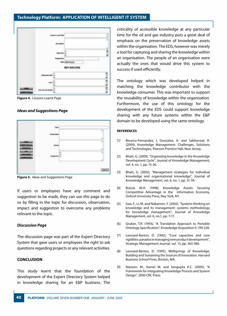
40 PLATFORM VOLUME SEVEN NUMBER ONE JANUARY - JUNE 2009
Technology Platform: APPLICATION OF INTELLIGENT IT SYSTEM
Ideas and Suggestions Page
If users or employees have any comment and suggestion to be made, they can use this page to do so by filling in the topic for discussion, observation, impact and suggestion to overcome any problems relevant to the topic.
Discussion Page
The discussion page was part of the Expert Directory System that gave users or employees the right to ask questions regarding projects or any relevant activities.
CONCLUSION
This study learnt that the foundation of the development of the Expert Directory System helped in knowledge sharing for an E&P business. The
criticality of accessible knowledge at any particular time for the oil and gas industry puts a great deal of emphasis on the preservation of knowledge assets within the organisation. The EDS, however was merely a tool for capturing and sharing the knowledge within an organisation. The people of an organisation were actually the ones that would drive this system to success if used efficiently.
The ontology which was developed helped in matching the knowledge contributor with the knowledge consumer. This was important to support the reusability of knowledge within the organisation. Furthermore, the use of this ontology for the development of the EDS could support knowledge sharing with any future systems within the E&P domain to be developed using the same ontology.
REFERENCES
[1] Becerra-Fernandez, I, Gonzalez, A. and Sabherwal, R. (2004), Knowledge Management: Challenges, Solutions and Technologies, Pearson Prentice Hall, New Jersey.
[2] Bhatt, G. (2000), “Organizing knowledge in the Knowledge Development Cycle”, Journal of Knowledge Management, vol. 4, no. 1, pp. 15-26.
[3] Bhatt, G. (2002), “Management strategies for individual knowledge and organisational knowledge”, Journal of Knowledge Management, vol. 6, no. 1, pp. 31-39.
[4] Boisot, M.H. (1998), Knowledge Assets: Securing Competitive Advantage in the Information Economy, Oxford University Press, Ney York, NY.
[5] Gao, F., Li, M. and Nakamori, Y. (2002), “Systems thinking on knowledge and its management: systems methodology for knowledge management”, Journal of Knowledge Management, vol. 6, no.1, pp. 7-17.
[6] Gruber, T.R. (1993), “A Translation Approach to Portable Ontology Specification”, Knowledge Acquisition 5: 199-220.
[7] Leonard-Barton, D. (1992), “Core capacities and core rigidities: paradox in managing new product development”, Strategic Management Journal, vol. 13, pp. 363-380.
[8] Leonard-Barton, D. (1995), Wellsprings of Knowledge: Building and Sustaining the Sources of Innovation. Harvard Business School Press, Boston, MA.
[9] Niessen, M., Kamel M, and Sengupta K.C. (2000), “A Framework for Integrating Knowledge Process and System Design”, 2000 CRC Press.
Figure 4. Lessons Learnt Page
Figure 5. Ideas and Suggestions Page

41 VOLUME SEVEN NUMBER ONE JANUARY - JUNE 2009 PLATFORM
Technology Platform: APPLICATION OF INTELLIGENT IT SYSTEM
[10] Nonaka, I. (1994), “A dynamic theory of organisational knowledge creation”, Organisation Science, vol. 5, no. 1, pp. 14-37.
[11] Nonaka, I. (2000), “SECI, Ba, and leadership: a unifying model of dynamic knowledge creation”, IMPM Seminar, JAIST.
[12] Noy, N. F. and McGuinness, D. (2000),”Ontology Development 101: A Guide to Creating Your First Ontology”, Stanford University, Stanford.
[13] Pralahad, C.K. and Hamel, G. (1990), “The core competence of the corporation”, Harvard Business Review, vol. 68, no. 3, pp. 79-93.
[14] Sharp, D. (2003), “Knowledge Management Today: Challenges and Opportunities”, Knowledge Management Today, pp. 32-37.
[15] Uschold, M and Gruniger, M. (1996), “Ontologies: Principles, Methods and Applications”, Knowledge Engineering Review
[16] Zúñiga, G.L. (2001), “Ontology: Its Transformation From Philosophy to Information Systems”, Proceedings of the International Conference on Formal Ontology in Information Systems, vol. 2001, ACM.
Ainol Rahmah Shazi Shaarani is currently a lecturer in Universiti Teknologi PETRONAS.
Mazeyanti M Ariffin is currently a lecturer in Universiti Teknologi PETRONAS. she teaches Knowledge Management and her research interest is game in knowledge management and knowledge transfer

42 PLATFORM VOLUME SEVEN NUMBER ONE JANUARY - JUNE 2009
Technology Platform: APPLICATION OF INTELLIGENT IT SYSTEM
INTRODUCTION
Missing attribute values is a common problem in knowledge discovery from data (KDD) processes. This problem may arise from collecting processes due to the device and human error. The quality of KDD depends on the quality of data. Ignoring the missing data may degrade the performance of KDD. Grzysmala-Busse and Hu [1] studied the comparison of several approaches to missing attribute values in data mining. Li and Cercone introduced a new approach RSFit and ItemRSFit on processing data with missing attribute values based on rough set theory (RST), distance based methods and association rules [2-4]. Troyanskaya, et al. [5] implemented and evaluated three methods for missing value estimation for DNA microarrays: a Singular Value Decomposition (SVD) based method (SVDImpute), weighted k-nearest neighbours (KNNImpute), and row average.
Bhattacharya, Shrestha and Solomatine [6] used ANN in reconstructing missing wave data in sedimentation modeling.
The curse of dimensionality is one of the damning factors for ANN to reach good performance [7]. Feature selection and attribute reduction are needed to overcome the problem of curse dimensionality. Li, Manry, Narasimha, and Yu [8] proposed piece-wise linear network using orthonormal least square (PLN-OLS) to rank and select features. Rough set theory also has the ability to reduce the dimensionality of attributes and to select features without loss of information by its reduct and core concepts [9].
ANN with RST attribute reduction is proposed in this research to predict the simulated missing attribute values on heart disease data from University of California Irvine (UCI) database. The accuracy of
MISSING ATTRIBUTE VALUE PREDICTION BASED ON ARTIFICIAL NEURAL NETWORK AND ROUGH SET THEORY
N.A. Setiawan* , P.A. Venkatachalam, Ahmad Fadzil Mohd Hani Universiti Teknologi PETRONAS, 31750 Tronoh, Perak Darul Ridzuan, Malaysia
ABSTRACT
In this research, artificial neural network (ANN) combined with rough set theory (RST), named as ANNRST, was proposed to predict missing values of attribute. The prediction of missing values of attribute was applied on heart disease data from UCI datasets. The ANN used was the multilayer perceptron (MLP) with resilient back-propagation learning. RST could reduce the dimensionality of attributes through its reduct. Reduct was used as input of ANN combined with decision attribute. By simulating missing values, the prediction accuracy of ANN was compared to ANNRST. The accuracy of ANNRST was also compared with missing data imputation of k-Nearest Neighbour (k-NN), most common attribute value method and ANN with piece-wise linear network-orthonormal least square feature selection (PLN-OLS). Simulation results showed that ANNRST could predict missing values with maximum accuracy close to ANN without dimensionality reduction (pure ANN) and outperformed k-NN, most common attribute value method, and ANN with PLN-OLS.
Keywords: neural network, rough set theory, missing value.
This paper was presented at the IEEE International Conference Biomedical Engineering & Informatics (BMEI), China 27 - 30 May 2008
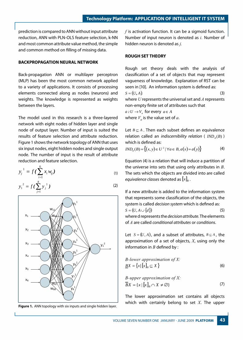
43 VOLUME SEVEN NUMBER ONE JANUARY - JUNE 2009 PLATFORM
Technology Platform: APPLICATION OF INTELLIGENT IT SYSTEM
prediction is compared to ANN without input attribute reduction, ANN with PLN-OLS feature selection, k-NN and most common attribute value method, the simple and common method on filling of missing data.
BACKPROPAGATION NEURAL NETWORK
Back-propagation ANN or multilayer perceptron (MLP) has been the most common network applied to a variety of applications. It consists of processing elements connected along as nodes (neurons) and weights. The knowledge is represented as weights between the layers.
The model used in this research is a three-layered network with eight nodes of hidden layer and single node of output layer. Number of input is suited the results of feature selection and attribute reduction. Figure 1 shows the network topology of ANN that uses six input nodes, eight hidden nodes and single output node. The number of input is the result of attribute reduction and feature selection.
∑=
=6
1
1j
iix ijwfy )( (1)
∑=
=8
1
121
jjyfy )( (2)
f is activation function. It can be a sigmoid function. Number of input neuron is denoted as i. Number of hidden neuron is denoted as j.
ROUGH SET THEORY
Rough set theory deals with the analysis of classification of a set of objects that may represent vagueness of knowledge. Explanation of RST can be seen in [10]. An information system is defined as:
( )AUS .= , (3)where U represents the universal set and A represents non-empty finite set of attributes such that
VUa a→: for every Aa∈where Va is the value set of a.
Let AB ⊆ . Then each subset defines an equivalence relation called an indiscernibility relation ( )(BINDA ) which is defined as:
( ) ( ) ( ){ }yaxaBaUyxBINDA =∈∀∈= ,|,)( 2 (4)
Equation (4) is a relation that will induce a partition of the universe into sets that using only attributes in B. The sets which the objects are divided into are called equivalence classes denoted as [ ]Bx .
If a new attribute is added to the information system that represents some classification of the objects, the system is called decision system which is defined as:
{ }( )dAUS ∪= , (5)where d represents the decision attribute. The elements of A are called conditional attributes or conditions.
Let ( ) , AUS = , and a subset of attributes, AB ⊆ , the approximation of a set of objects, X, using only the information in B defined by :
B-lower approximation of X:[ ]{ }XxxXB B ⊆= | (6)
B-upper approximation of X:[ ] }|{ ∅≠∩= XxxXB B
(7)
The lower approximation set contains all objects which with certainly belong to set X. The upper
Figure 1. ANN topology with six inputs and single hidden layer.
x1
x2
x3
x4
x5
x6
y11
y21
w11
w12
y31
y41
y51
y61
y71
y81
y12
w68
w67

44 PLATFORM VOLUME SEVEN NUMBER ONE JANUARY - JUNE 2009
Technology Platform: APPLICATION OF INTELLIGENT IT SYSTEM
approximation set contains all objects which possibly belong to the set X.
B-boundary region of X:XBXBXBRB −=)( (8)
This set contains the objects that cannot be classified as definitely inside X nor definitely outside X. A set is rough if ∅≠)(XBRB .
Sometimes all the knowledge in an information system is necessary to divide the object into classes. In this case the knowledge can be reduced. Reducing the knowledge results in reducts. A reduct is a minimal set of attributes AB ⊂ , such that
)()( AINDBIND AA = (9)
Reducts can be computed based on discernibility matrices and discernibility function. A discernibility matrix of information system S is a symmetric nn× matrix with entries:
( ) ( ),...,1,for
|
nji
xaxaAac jiij
=≠∈=
(10)
A discernibility function fA for an information system S is a Boolean function of m Boolean variables **
1 ,..., maa (corresponding to the attributes maa ,...,1 ) defined as
{ }∅≠≤≤≤∨∧= ijij
mA
cnijc
aaf
,1|
),...,(*
**1
(11)
where }|{ **ijij caac ∈= . By finding the set of all
prime implicants of the discernibility function, all the minimal reduct of the system may be determined.
For decision systems S, finding an approximation of the decision, d can be done by constructing its decision-relative discernibility matrix. The process of computing this matrix is called computing the discernibility matrix modulo the decision attribute.
If )()( ijcAM = is the discernibility matrix of a decision system S, the decision-relative discernibility matrix of defined as:
)()( dij
d cAM = with assumption of ∅=dijc if
)()( ji xdxd = and dcc ijdij −= otherwise.
In this research, the concept of reduct was used to reduce the dimension of input attributes for ANN.
COMBINED SYSTEM (ANNRST)
RST is used to reduce the input of ANN. For example of heart disease problem, before attribute reduction, there is ten input attributes. Using RST reduct concept, the number of input can be reduced to less than ten, e.g., six attributes. Thus the input of ANN is reduced. The topology of ANNRST can be seen in Figure 2.
X1 - Xm are inputs of ANN before RST attribute reduction. X’1-X’n are inputs of ANN after attribute reduction and m > n.
EXPERIMENT AND RESULTS
Data and preprocessing
The source of the heart (coronary artery) disease data was from a data mining repository at UCI [11]. The amount of data was 920 instances. The cleveland data was the most complete. The swiss data was the most incomplete, thus it was not used in this research. The longbeach and hungarian data had many missing
RST Attribute Reducer
X1 X2 X3 Xm-2 Xm-1 Xm
X’1 X’2 X’n-1 X’n
ANN
Figure 2. ANNRST topology with single hidden layer.

45 VOLUME SEVEN NUMBER ONE JANUARY - JUNE 2009 PLATFORM
Technology Platform: APPLICATION OF INTELLIGENT IT SYSTEM
values in three of thirteen conditional attributes (the three attributes was removed). The original data had thirteen conditional attributes and a single decision attribute. Only ten conditional attributes were used in this research due to the completeness of data.
Preprocessing was by removing the instance with too many missing values and by removing outliers based on statistical mean and standard deviation. 597 instances were available after preprocessing. The final attributes are shown in Table 1. The diagnosis of coronary artery disease is the decision attributes. Discretisation was conducted using Boolean reasoning.
Simulation of missing value and reduct computation
Missing values were simulated arbitrarily for the fbs attribute by removing its values. Ten to 90 values were removed from 597 instances on the fbs attribute and treated as missing values.
Reduct computation using ROSETTA [12] with Boolean reasoning discretisation and Johnson’s algorithm resulted in reduct with five attributes: age, trestbps, chol, thalach and oldpeak.
Experiment
ANN was used to predict the simulated missing values on fbs attribute.
Pure ANN uses ten input nodes. ANN with RST (ANNRST) dimensionality reduction and PLN-OLS attribute ranking (ANN-PLN-OLS) use six input nodes. Attributes used for ANNRST are attributes of the computed reduct and decision attribute (num). Attributes based on PLN-OLS feature ranking using six attributes are thalach, cp, age, restecg, trestbps and oldpeak.
Ten to ninety simulated missing values of fbs attribute were predicted using pure ANN, ANNRST and ANN-PLN-OLS. Hundreds of simulations with random initial weights were conducted, each simulated with missing
data using MATLAB with Nguyen-Widrow weight initialisation, minmax scaling, resilient bacpropagation training, and tansig activation function at hidden and output layer. K-NN imputation method and most
Table 1. Summary of attributes (UCI heart disease database)
Attribute Description Value descriptionage Age Numerical valuesex Sex 1 if male;
0 if femalecp Chest pain type 1 typical angina
2 atypical angina
3 non-anginal pain
4 asymptomatictrestbps Resting systolic
blood pressure on admission to the hospital (mmHg)
Numerical value
chol Serum cholesterol (mg/dl)
Numerical value
fbs Fasting blood sugar over 120 mg/dl ?
1 if yes0 if no
restecg Resting electro-cardiographic results :
0 normal1 having
ST-T wave abnormality
2 LV hypertrophy
thalach Maximum heart rate achieved
Numerical value
exang Exercise induced angina?
1 if yes0 if no
oldpeak ST depression induced by exercise relative to rest
Numerical value
num Diagnosis of heart disease (angiographic disease status/ presence of coronary artery disease (CAD))
0 if less than 50% diameter narrowing in any major vessel (CAD no)
1 if more than 50% (CAD yes)
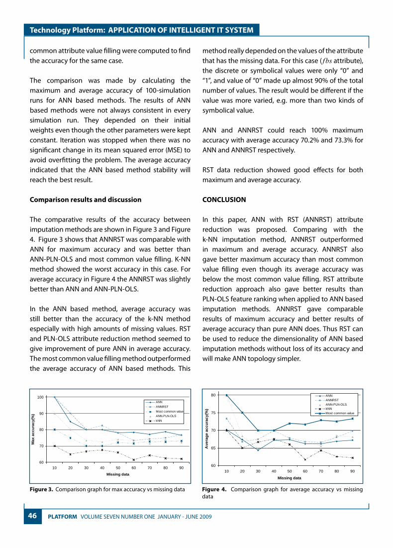
46 PLATFORM VOLUME SEVEN NUMBER ONE JANUARY - JUNE 2009
Technology Platform: APPLICATION OF INTELLIGENT IT SYSTEM
common attribute value filling were computed to find the accuracy for the same case.
The comparison was made by calculating the maximum and average accuracy of 100-simulation runs for ANN based methods. The results of ANN based methods were not always consistent in every simulation run. They depended on their initial weights even though the other parameters were kept constant. Iteration was stopped when there was no significant change in its mean squared error (MSE) to avoid overfitting the problem. The average accuracy indicated that the ANN based method stability will reach the best result.
Comparison results and discussion
The comparative results of the accuracy between imputation methods are shown in Figure 3 and Figure 4. Figure 3 shows that ANNRST was comparable with ANN for maximum accuracy and was better than ANN-PLN-OLS and most common value filling. K-NN method showed the worst accuracy in this case. For average accuracy in Figure 4 the ANNRST was slightly better than ANN and ANN-PLN-OLS.
In the ANN based method, average accuracy was still better than the accuracy of the k-NN method especially with high amounts of missing values. RST and PLN-OLS attribute reduction method seemed to give improvement of pure ANN in average accuracy. The most common value filling method outperformed the average accuracy of ANN based methods. This
method really depended on the values of the attribute that has the missing data. For this case ( fbs attribute), the discrete or symbolical values were only “0” and “1”, and value of “0” made up almost 90% of the total number of values. The result would be different if the value was more varied, e.g. more than two kinds of symbolical value.
ANN and ANNRST could reach 100% maximum accuracy with average accuracy 70.2% and 73.3% for ANN and ANNRST respectively.
RST data reduction showed good effects for both maximum and average accuracy.
CONCLUSION
In this paper, ANN with RST (ANNRST) attribute reduction was proposed. Comparing with the k-NN imputation method, ANNRST outperformed in maximum and average accuracy. ANNRST also gave better maximum accuracy than most common value filling even though its average accuracy was below the most common value filling. RST attribute reduction approach also gave better results than PLN-OLS feature ranking when applied to ANN based imputation methods. ANNRST gave comparable results of maximum accuracy and better results of average accuracy than pure ANN does. Thus RST can be used to reduce the dimensionality of ANN based imputation methods without loss of its accuracy and will make ANN topology simpler.
Figure 3. Comparison graph for max accuracy vs missing data Figure 4. Comparison graph for average accuracy vs missing data
60
70
80
90
100
10 20 30 40 50 60 70 80 90
Miss ing data
Max
acc
ura
cy(%
)
ANN
ANNRST
Most common value
ANN-PLN-OLS
kNN
60
65
70
75
80
10 20 30 40 50 60 70 80 90
Miss ing data
Ave
rag
e ac
cura
cy(%
)
ANNANNRSTANN-PLN-OLSkNNMost common value

47 VOLUME SEVEN NUMBER ONE JANUARY - JUNE 2009 PLATFORM
Technology Platform: APPLICATION OF INTELLIGENT IT SYSTEM
ACKNOWLEDGMENTWe would like to thank Universiti Teknologi PETRONAS for the kind support of presenting this paper at BMEI 2008.
REFERENCES
[1] J.W. Grzysmala-Busse, M. Hu, “A comparison of several approaches to missing attribute values in data mining”, RSCTC 2000, LNAI, 2005, pp. 378- 385.
[2] J. Li, N. Cercone, Comparisons on different approaches to assign missing attribute values, Technical Report, CS-2006-04, School of Computer Science, University of Waterloo, January 2006.
[3] J. Li, N. Cercone,”Assigning missing attribute values based on rough set theory”, IEEE GrC 2006, Atlanta USA, May 2006.
[4] J. Li, N. Cercone, Predicting missing attribute values based on Frequent Itemset and RSFit, Technical Report, CS-2006-13, School of Computer Science, University of Waterloo, April 2006.
[5] O. Troyanskaya, M. Cantor, G. Sherlock, P. Brown, T. Hastie, R. Tibshirani, D. Botstein, R.B. Altman, “Missing value estimation methods for DNA microarrays”, Bioinformatics 17(6), 2001, pp. 520-525.
[6] B. Bhattacharya, D.L. Shrestha, D.P. Solomatine, “Neural networks in reconstructing missing wave data in sedimentation modeling”, Proceedings of the XXXth IAHR Congress, Greece, August 2003.
[7] C.M. Bishop, Neural Networks for Pattern Recognition, Oxford University Press, 1994.
[8] J. Li, M.T. Manry, P.L. Narashima, C. Yu, “Feature selection using a piecewise linear network”, IEEE Transaction on Neural Networks, 17(5), September 2006, pp. 1101-1115.
[9] Q. Shen, A. Chouchoulas, “Rough set-based dimensionality reduction for supervised and unsupervised learning”, Int. J. Appl. Math. Comput. Sci., Vol.11, 2001, pp. 583-601.
[10] T.R. Hvidsten, Fault diagnosis in rotating machinery using rough set theory and ROSETTA, Technical Report, Norwegian University of Science and Technology, 1999.
[11] D.J. Newman, S. Hettich, , C.L. Blake, C.J. Merz, UCI Repository of machine learning databases http://www.ics.uci.edu/~mlearn/MLRepository.html. Irvine, CA: University of California, Department of Information and Computer Science. 1998
[12] A. Ohrn., ROSETTA,http://www.idi.ntnu.no/~aleks/ro-setta, 1999.
P. A. Venkatachalam received his Bachelors Degree in Electrical and Electronics Engineering with First Class Honours. He read for his Masters in MTech (Control System Engineering) from the Indian Institute of Technology, Kharagpur and his PhD (Computer Engineering and Science Software Engineering) from the Indian Institute of Technology, Kanpur. He
startedhis career as an Electrical Engineer (1957-61) and later, served in the Indian Government as a lecturer (1961-66) and Assistant Professor (1966-76). He held the position of Full Professor at the Asian Institute of Technology, Bangkok (2 years) and at Anna University, Madras, India (10 years) where he was also the Head of its Department of Electronics, Communication & Computer Science & Engineering. From 1988-2000, he served as Professor at Universiti Sains Malaysia (1988-2000). Currently, he is a Professor at the Electrical & Electronics Enginering Program, Universiti Teknologi PETRONAS. His areas of research are in Software Engineering, Computer Networks, Image Processing, Medical Imaging and IT.
Ahmad Fadzil M. H. graduated in 1983 from the University of Essex, UK with a BSc (First Class Honours) in Electronic Engineering. He obtained his MSc in Telematics in 1984 and PhD in Image Processing in 1991 from the same university.He was a Lecturer in Signal Processing and Researcher in Image Processing at the Universiti Sains Malaysia
(USM) from 1984 till 1996. While on doctoral study leave between 1988 and 1991, he was appointed by University of Essex, UK initially as a Senior Research Officer in Image Processing and subsequently as a Lecturer. In 1992, he was appointed Dean, School of Electrical & Electronic Engineering, Universiti Sains Malaysia (USM) and in 1994, he was promoted to Associate Professor. In 1997, he joined Universiti Teknologi PETRONAS (UTP) as the Dean of the Engineering Faculty. He was appointed the Director of Academic Studies in 1999 and later as the Director of Postgraduate Studies in 2003. In 2006, he was promoted to a full Professor and currently leads a research cluster in intelligent signal & imaging systems.
Prof. Ir Dr Ahmad Fadzil is a Fellow and a former Council Member of the Institution of Engineers, Malaysia. He is a registered Professional Engineer with the Board of Engineers, Malaysia. He is also a Senior Member of the Institute of Electrical & Electronic Engineers Inc (IEEE), USA. He is an appointed member of Engineering Accreditation Council, Board of Engineers Malaysia. He is actively involved with the industry as a member of the Board of Directors of a public-listed R&D company that develops and manufactures automated vision inspection systems. He has published over 80 research articles in conference proceedings and journals. His research interests include image coding, medical imaging and telemedicine for healthcare, vision inspection systems, and signal processing of seismic data for hydrocarbon exploration.

48 PLATFORM VOLUME SEVEN NUMBER ONE JANUARY - JUNE 2009
Technology Platform: FUEL COMBUSTION
INTRODUCTION
Combustion of fuel sprays is a very important area in gas turbines, diesel and spark ignition engines, furnaces and hazardous environments. However, the exploration of important parameters in practical combustion systems is difficult due to the multiplicity of dependent variables such as spatial variations in pressure, temperature, equivalence ratio, and droplet sizes. Thus, fundamental study on the influence of the presence of liquid droplets in aerosol flames is vital before the behaviour of practical spray combustion can be fully understood. Information on laminar burning velocity of aerosol flames is sparse, even for gaseous mixtures at conditions pertaining to engines, which range from sub-atmospheric to high pressure and temperature.
Theoretical [1, 2] and experimental [3-5] studies suggested that laminar flame propagation through aerosol/vapour clouds, under certain circumstances,
is higher than that in a fully vapourised homogeneous mixture. However, there is little experimental data of a fundamental nature that demonstrates the similarities and differences in burning rate of turbulent flames between single and two-phase combustion. Myers and Lefebvre [3] investigated the influence of mean droplet size and mainstream velocity on flame speed using mixtures of JP 7 fuel drops and air in a circular duct. They suggested that the enhanced flame speed with an increase in the mainstream velocity was a result of increase in the associated turbulence intensity. In various researches, it was reported that the turbulent flame speed was inversely proportional with the mean droplet size [3, 4, 6-8]. The droplet evaporation rates were suggested to control the turbulent flame speed [3, 7]. However, El-Banhawy and Whitelaw [7] also suggested that droplet evaporation would only have an influence on the combustion process if a time characteristic of the turbulent mixing between fuel and air were comparable to that which characterizes droplets evaporation.
BURNING RATES OF TURBULENT GASEOUS AND AEROSOL FLAMES
Shaharin A. Sulaiman* and Malcolm LawesUniversiti Teknologi PETRONAS, 31750 Tronoh, Perak Darul Ridzuan, Malaysia
ABSTRACT
It has been revealed that laminar flames within aerosol mixtures become unstable more readily than gaseous flames and this increases the practical burning rate. However, studies on turbulent flames of aerosol mixtures of mono-dispersed droplets are limited. In this study, centrally ignited expanding flames were employed to quantify the burning rates in gaseous and aerosol flames. Iso-octane-air aerosols were generated by expansion of the gaseous pre-mixture to produce a homogeneously distributed suspension of fuel droplets. The effects of the presence of droplets and turbulence velocity in relation to the burning rates of the flame were also investigated.
Keywords: Burning Rate, Droplets, Flames, Turbulent
This paper was presented at the International Conference on Mechanical Engineering, Tokyo 27 - 29 May 2009
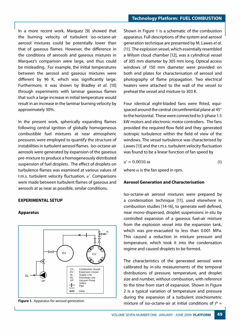
49 VOLUME SEVEN NUMBER ONE JANUARY - JUNE 2009 PLATFORM
Technology Platform: FUEL COMBUSTION
In a more recent work, Marquez [9] showed that the burning velocity of turbulent iso-octane-air aerosol mixtures could be potentially lower than that of gaseous flames. However, the difference in the conditions of aerosols and gaseous mixtures in Marquez’s comparison were large, and thus could be misleading. For example, the initial temperatures between the aerosol and gaseous mixtures were different by 96 K, which was significantly large. Furthermore, it was shown by Bradley et al. [10] through experiments with laminar gaseous flames that such a large increase in initial temperature would result in an increase in the laminar burning velocity by approximately 30%.
In the present work, spherically expanding flames following central ignition of globally homogeneous combustible fuel mixtures at near atmospheric pressures were employed to quantify the structure of instabilities in turbulent aerosol flames. Iso-octane-air aerosols were generated by expansion of the gaseous pre-mixture to produce a homogeneously distributed suspension of fuel droplets. The effect of droplets on turbulence flames was examined at various values of r.m.s. turbulent velocity fluctuation, u’. Comparisons were made between turbulent flames of gaseous and aerosols at as near as possible, similar conditions.
EXPERIMENTAL SETUP
Apparatus
Shown in Figure 1 is a schematic of the combustion apparatus. Full descriptions of the system and aerosol generation technique are presented by M. Lawes et al. [11]. The explosion vessel, which essentially resembled a Wilson cloud chamber [12], was a cylindrical vessel of 305 mm diameter by 305 mm long. Optical access windows of 150 mm diameter were provided on both end plates for characterisation of aerosol and photography of flame propagation. Two electrical heaters were attached to the wall of the vessel to preheat the vessel and mixture to 303 K.
Four identical eight-bladed fans were fitted, equi-spaced around the central circumferential plane at 45° to the horizontal. These were connected to 3-phase 1.5 kW motors and electronic motor controllers. The fans provided the required flow field and they generated isotropic turbulence within the field of view of the windows. The vessel turbulence was characterised by Lawes [13] and the r.m.s. turbulent velocity fluctuation was found to be a linear function of fan speed by
ω0.0016' =u (1)
where ω is the fan speed in rpm.
Aerosol Generation and Characterisation
Iso-octane-air aerosol mixtures were prepared by a condensation technique [11], used elsewhere in combustion studies [14-16], to generate well defined, near mono-dispersed, droplet suspensions in-situ by controlled expansion of a gaseous fuel-air mixture from the explosion vessel into the expansion tank, which was pre-evacuated to less than 0.001 MPa. This caused a reduction in mixture pressure and temperature, which took it into the condensation regime and caused droplets to be formed.
The characteristics of the generated aerosol were calibrated by in-situ measurements of the temporal distributions of pressure, temperature, and droplet size and number, without combustion, with reference to the time from start of expansion. Shown in Figure 2 is a typical variation of temperature and pressure during the expansion of a turbulent stoichiometric mixture of iso-octane-air at initial conditions of P = Figure 1. Apparatus for aerosol generation
CV : Combustion Vessel EV : Expansion Vessel SL : Supply Line DL: Discharge Line VP: Vacuum Pump Orifice Pipe
Valve
DL
VP
CV EV
SL

50 PLATFORM VOLUME SEVEN NUMBER ONE JANUARY - JUNE 2009
Technology Platform: FUEL COMBUSTION
200 kPa, T = 303 K and u’ = 1.0 m/s. The fluctuations in the measurements were the effect of electronic signal noise caused by the fan motors. The expansion process took place in less than one second. The temperature of the mixture dropped to a value of lower than –10°C.
The droplet arithmetic mean diameter, D10, was measured using a Phase Doppler Anemometer (PDA) system. The number density of droplets, ND, was estimated from laser extinction measurement during expansion by using the Beer-Lambert Law correlation given in S. Hayashi and S. Kumagai, [17]. Because expansion took place over a period of several seconds while combustion took place over less than 30 ms, the far field values of D10 were assumed to be constant during combustion. Detailed descriptions of the techniques for characterisation of the mixture droplets were published elsewhere [11].
Shown in Figure 3 is the variation of droplet size and number density of droplets with time from the start of expansion from the same experiment as in Figure 2. Droplet nucleation started approximately 0.2 s after the expansion, as evident by the increase in D. It is shown that ND is consistently in the order of 1010 m-3, immediately after the start of condensation. Clearly, the distribution of droplet size that results in the present apparatus is shown in Figure 3 to be near mono-dispersed at between about 0.2 and 0.4 s after the onset of droplet nucleation. This is also supported by the typical histogram in Figure 4, which shows a narrow droplet distribution at 0.25 seconds after the start of expansion. The spatial distribution of droplet size was also monitored and was found to be reasonably uniform [9].
Recording of Flame Images
The aerosol mixture was ignited at the centre of the explosion vessel by an electric spark of about 500 mJ. The flame front was monitored through the vessel’s windows by Schlieren movies, which were recorded using a high speed digital camera at a rate of 1000 frames per second and with a resolution of 256 pixels × 256 pixels. The flame image was processed digitally
Figure 3. Variation of droplet size, D, and droplet number density, ND , during the expansion of a turbulent mixture of iso-octane-air.
Figure 4. Typical histogram for droplet diameter distributions for turbulent iso-octane-air aerosol mixture in Figure 3 at time of 0.25 ± 0.005 s after start of expansion.
Figure 2. Typical variation of temperature and pressure during the expansion of a turbulent mixture of iso-octane-air
0
50
100
150
200
250
0.0 0.2 0.4 0.6 0.8 1.0
Time from start of expansion (s)
Pre
ssur
e (k
Pa)
-20
-10
0
10
20
30
40
Tem
pera
ture
(°C
)
P
T
0
5
10
15
20
25
30
35
0.1 0.2 0.3 0.4 0.5 0.6
Time from start of expansion (s)
Dro
plet
Dia
mete
r (m
icro
ns)
.
1.E+06
1.E+07
1.E+08
1.E+09
1.E+10
1.E+11
1.E+12
Est
imat
ed d
ropl
et n
umbe
r den
sity
(m -3
)
D
ND
0
10
20
30
40
50
60
70
80
90
2 4 6 8 10 12 14 16
Droplet Diameter (microns)
Fre
quen
cy (
%)

51 VOLUME SEVEN NUMBER ONE JANUARY - JUNE 2009 PLATFORM
Technology Platform: FUEL COMBUSTION
to obtain the radius of the flame front, r, by using image-processing software described in [18].
The flame speed, St , was obtained from the measured flame front radius against time by
dt
drSt = (2)
RESULTS AND DISCUSSIONS
The effect of droplets on turbulence aerosol flames was examined by comparing the burning rates with those of turbulent gaseous flames. Comparison was also made for experiments at various values of u’.
Observation of Flames
Shown in Figure 5 are typical Schlieren images of turbulent flames for stoichiometric iso-octane-air aerosol mixtures at P = 128 kPa, T = 283 K, D10 = 4 µm and u’ of (a) 1.0 m/s and (b) 2.5 m/s. The circular boundary represents the 150-mm diameter field of view of the camera as determined by the optical access windows and Schlieren setting. The black horizontal object in each of the photographs is the spark electrode holder. In general, it is shown in Figure 5 that turbulent flames wrinkle and deform considerably as compared to the nearly spherical laminar flames of aerosol mixtures [19]. The degree of wrinkling is also shown qualitatively to increase with u’. The Schlieren images of turbulent gaseous flames (not shown) at similar conditions using the same experiment rig were found to be similar to those for the aerosol mixtures. For aerosol with larger droplets (D10 > 4 µm) the mixtures failed to ignite, probably due to the need for higher ignition energy.
Effect of Presence of Droplets
Shown in Figure 6 is the variation of radius with time for stoichiometric iso-octane-air mixtures at u’ of 1.0 m/s. The triangular markers represent the results for gaseous mixtures at P = 100 kPa and T = 303 K; the circles represent those for aerosol mixtures at P = 128 kPa, T = 283 K and D10 = 4 µm. The slight difference in pressure and temperature for the different flames
Figure 6. Variations of flame radius with time for turbulent mixtures of stoichiometric iso-octane-air at u’ of 1.0 m/s.
(a) u’ = 1.0 m/s
(b) u’ = 2.5 m/s
Figure 5 Typical Schlieren images of turbulent flames in stoichiometric iso-octane-air aerosols using the same spark electrode and energy.
0
10
20
30
40
50
60
0 5 10 15 20 25
Time (ms)
Rad
ius
(mm
) .
`
Gaseous
Aerosol

52 PLATFORM VOLUME SEVEN NUMBER ONE JANUARY - JUNE 2009
Technology Platform: FUEL COMBUSTION
was unavoidable and was due to the method of thermodynamic aerosol generation; this was described in [20]. The gaseous (single phase) flames could not be studied within the range of pressures and temperatures of aerosols because at such conditions the mixture would be in the wet, or two-phase, regime. However, Bradley et al. [10] showed that, for gaseous flames, such small differences in pressure and temperature have little effect on the burning rate. For each condition, up to five explosions were plotted. The fluctuation in the results was found to be low for small flame kernels (r < 10 mm) but gradually increased with time, possibly due to the effect of large turbulent eddies. It is shown in Figure 6 that the radii for both aerosol and gaseous flames were nearly identical during the first 5 ms of the flame development. Thereafter, the radius of the turbulent gaseous flames is shown to be always higher than that of aerosol flames.
Shown in Figure 7 is the resulting turbulent flame speed, plotted against time after ignition, for the mixtures in Figure 6. The turbulent flame speed was obtained using Eq. (2). In Figure 7, the variation of turbulent flame speed is plotted against the flame radius. The fluctuation in the results is within a maximum value of less than 1.0 m/s. The turbulent flame speed of the gaseous mixtures is shown in Figures 7 and 8 as identical with that of the aerosol mixture during the first 5 ms of the flame development. This was most probably because the energy for the flame kernel was contributed mainly by the spark ignition. A regime of flame development [21] for laminar flames is also exhibited in Figures 7 and 8 during the start of ignition. The flame speed was relatively high as a result of active radicals provided by the spark energy. However, high stretch rates of the flames caused the flame speed to decrease rapidly when the thermal energy of the spark was dissipated into the reactant and before normal flame chemistry developed.
The general trend in Figures 7 and 8 is a sustained increase in St with time and radius with no evidence of flame speed stabilization as was observed for the laminar cases [19]. Obviously the gaseous flames in Figure 7 exhibited a higher acceleration rate at
0
1
2
3
4
5
6
0 5 10 15 20 25
Time (ms)
S t (
m/s
)
Gaseous
Aerosol
0
1
2
3
4
5
6
0 10 20 30 40 50
Radius (mm)
S t (
m/s
)
Gaseous
Aerosol
0
1
2
3
4
5
6
0 5 10 15 20 25
Time (ms)
S t (
m/s
)
u' = 2.5 m/s
u' = 1.5 m/s
u' = 1.0 m/s
Figure 7. Variations of turbulent flame speed with time for the mixtures in Figure 6.
Figure 8. Variations of turbulent flame speed with radius for the mixtures in Figure 6.
Figure 9 Variation of St with time for turbulent flames of stoichiometric iso-octane aerosol ignited at D10 = 4 µm, and u’ of 1.0, 1.5 and 2.5 m/s.

53 VOLUME SEVEN NUMBER ONE JANUARY - JUNE 2009 PLATFORM
Technology Platform: FUEL COMBUSTION
between 5 and 10 ms after the start of ignition, resulting in a distinct separation between the plots for gaseous and aerosol flames. During this period, the effect from the spark had decayed and therefore further flame propagation depended on the readiness of the fuel-air mixtures to burn. Droplets in the aerosol mixtures required more time to sustain the chemical reaction as they needed to evaporate first, as compared to the gaseous mixtures, and this explains the reason for the faster burning rate of gaseous flames. Interestingly after 10 ms, the gradients of the graphs were quite parallel. This implies a possibility that the rate of acceleration for turbulent flame of gaseous and aerosol mixtures were similar after 10 ms; the same trend is also exhibited in Figure 8. Although the aerosol flames are shown to always have lower flame speeds, this was mainly the result of slow reactions at the initial stage of the flame development (<10 ms). If this effect of slow initial reaction in aerosol flames were absent, it is probable that the plot for the turbulent flames of gaseous and aerosol mixtures would be identical.
In the present work, the effect of droplet size, which was observed as a contributor to instabilities in laminar flames [11], could not be shown. Although, as indicated in Figure 3, near mono-dispersed droplets could be generated up to about 20 µm, the experiments were limited to small droplets (4 µm). This was because the energy required to ignite aerosols of large droplet would be higher, as reported in Sulaiman [20].
Effect of R.M.S. Turbulence Velocity Fluctuation
To demonstrate the effect of r.m.s. turbulent velocity fluctuation, u’, the explosion experiments were repeated at the same conditions of turbulent iso-octane aerosol mixtures (stoichiometric, P = 128 kPa, T = 283 K, D10 = 4 µm) but at different values of u’. The results are shown in Figures 9 and 10, in terms of St versus time and radius, respectively, for u’ of 1.0 m/s (circles), 1.5 m/s (crosses) and 2.5 m/s (squares). For each condition, a minimum of three explosions is plotted.
The trends for the turbulent aerosol flames in Figures 9 and 10 are similar to those for the flames in Figures 7 and 8, in which St increases with time and radius. The spark-affected flame behavior during the first 5 ms, as in Figures 7 and 8, is also shown in Figure 9 and 10. The flame growth rates for the aerosol mixtures are shown to increase with u’ ; and the trend is similar to that for turbulent gaseous flames as reported by Ormsby [22]. In addition, Figures 9 and 10 show that a larger scatter of results were found for turbulent aerosol flames at the higher turbulence as compared to the lower one, which was most probably the effect of turbulence velocity fluctuation.
It is shown in Figures 9 and 10 that during the initial kernel growth period, some of the flames had near zero values of St . These very slow initial propagation rates were probably due to the phenomenon described by Maly [23] as the random transport of the ignition kernel, due to flow field, towards the electrode, which consequently increased the heat loss from the flame kernel to the spark plug.
CONCLUSION
The effects of droplets and r.m.s. turbulent velocity fluctuation, u’, have been experimentally studied in centrally ignited spherical turbulent aerosol flames. Comparison of results was made with those for turbulent gaseous flames. Inspection of Schlieren cine-photographs revealed that turbulent aerosol
Figure 10 Variation of St with radius for the turbulent flames in Figure 9.
0
1
2
3
4
5
6
0 10 20 30 40 50
Radius (mm)
St (
m/s
)
u' = 1.0 m/s
u' = 1.5 m/s
u' = 2.5 m/s

54 PLATFORM VOLUME SEVEN NUMBER ONE JANUARY - JUNE 2009
Technology Platform: FUEL COMBUSTION
flames wrinkled and deformed significantly as compared to laminar aerosol flames. The effect was shown more obviously with an increase in u’.
The flame propagation rate of turbulent aerosol flames was shown to be slower than that of turbulent gaseous flames. This was probably caused by the longer time taken by aerosol flames during ignition due to the need to evaporate the droplets. However, after the flames had become fully developed, the rate of flame acceleration for the turbulent aerosol flames was shown to be similar with that of turbulent gaseous flames. As in gaseous flames, an increase in the r.m.s. turbulent velocity fluctuation increased the turbulent flame speed of the aerosol flames. A study on the effect of droplet size by using larger spark energy is recommended in the future.
ACKNOWLEDGMENT
The authors would like to acknowledge Universiti Teknologi PETRONAS, Malaysia, for its support in this work.
REFERENCES
[1] J. B. Greenberg, “Propagation and Extinction of an Unsteady Spherical Spray Flame Front,” Combust. Theory Modelling, vol. 7, pp. 163-174, 2003.
[2] T. H. Lin and Y. Y. Sheu, “Theory of Laminar Flame Propagation in Near-Stoichiometric Dilute Sprays, Combustion and Flame,” Combustion and Flame, pp. 333, 1991.
[3] G. D. Myers and A. H. Lefebvre, “Propagation in Heterogeneous Mixtures of Fuel Drops and Air,” Combustion and Flame, vol. 66, pp. 193-210, 1986.
[4] G. A. Richards and A. H. Lefebvre, “Turbulent Flame Speeds of Hydrocarbon Fuel Droplets in Air,” Combustion and Flame, vol. 78, pp. 299-307, 1989.
[5] D. R. Ballal and A. H. Lefebvre, “Flame Propagation in Heterogeneous Mixtures of Fuel Droplets, Fuel Vapor and Air,” Proc. Combust. Inst., 1981.
[6] Y. Mizutani and A. Nakajima, “Combustion of Fuel Vapour-Drop-Air Systems: Part II, Spherical Flames in a Vessel,” Combustion and Flame, vol. 21, pp. 351-357, 1973.
[7] Y. El-Banhawy and J. H. Whitelaw, “Experimental Study of the Interaction Between a Fuel Spray and Surrounding Combustion Air,” Combustion and Flame, vol. 42, pp. 253-275, 1981.
[8] S. H. Stårner, J. Gounder, and A. R. Masri, “Effects of Turbulence and Carrier Fluid on Simple, Turbulent Spray Jet Flames,” Combustion and Flame, vol. 143, pp. 420-432, 2005.
[9] N. Marquez, Fundamental Studies of Aerosol Flames, PhD Thesis, School of Mechanical Engineering, University of Leeds, UK, 2003.
[10] D. Bradley, R. A. Hicks, M. Lawes, C. G. W. Sheppard, and R. Woolley, “The Measurement of Laminar Burning Velocities and Markstein Numbers of Iso-Octane-Air and Iso-Octane-n-Heptane-Air Mixtures at Elevated Temperatures and Pressures in an Explosion Bomb,” Combustion and Flame, vol. 115, pp. 126-144, 1998.
[11] M. Lawes, Y. Lee, and N. Marquez, “Comparison of Iso-octane Burning Rates between Single-phase and Two-phase Combustion for Small Droplets,” Combustion and Flame, vol. 144, pp. 513-525, 2006.
[12] C. T. R. Wilson, “Condensation of Water Vapour in the Presence of Dust-Free Air and Other Gases,” Proc. of the Royal Society of London, 1897.
[13] M. Lawes, Effects of Turbulence on Combustion in Engines, PhD Thesis, School of Mechanical Engineering, University of Leeds, 1987.
[14] K. Nakabe, Y. Mizutani, F. Akamatsu, M. Fuchihata, and S. H. ElEmam, “Spark-Ignited Spherical Flames Propagating in a Suspended Droplet Cloud,” 5th International Conference on Liquid Atomization and Spray Systems (ICLASS-91), 1991.
[15] S. Hayashi and S. Kumagai, “Flame Propagation in Fuel Droplet-Vapor-Air Mixtures,” Proc. Combustion Institute, 1974.
[16] S. Hayashi, S. Kumagai, and T. Sakai, “Propagation Velocity and Structure of Flames in Droplet-Vapor-Air Mixtures,” Combustion Science & Technology, vol. 15, pp. 169-177, 1976.
[17] W. D. Bachalo, A. B. Rosa, and S. V. Sankar, Diagnostic for Fuel Spray Characterization, in Combustion Measurements, N. Chigier, Ed., New York, Hemisphere, 1991.
[18] S. A. Sulaiman, M. Lawes, S. Hassan, and Z. A. Abdulkarim, “High-Speed Schlieren Imaging of Spherically Propagating Laminar Flames of Iso-Octane-Air Aerosol Mixtures,” 3rd World Engineering Congress, Penang, 2007.
[19] S. A. Sulaiman and M. Lawes, “High-Speed Schlieren Imaging and Post-Processing for Investigation of Flame Propagation within Droplet-Vapour-Air Fuel Mixtures,” IEM Journal, vol. 69, pp. 53-60, 2008.
[20] S. A. Sulaiman, Burning Rates and Instabilities in the Combustion of Droplet and Vapour Mixtures, PhD Thesis, Department of Mechanical Engineering, University of Leeds, UK, 2006.

55 VOLUME SEVEN NUMBER ONE JANUARY - JUNE 2009 PLATFORM
Technology Platform: FUEL COMBUSTION
[21] Y. Ali, D. Bradley, M. Lawes, and E. M. J. Mushi, “Problems of the Measurement of Markstein Lengths with Explosion Flames,” The Combustion Institute, Proceedings of the British and German Sections, Queen’s College Cambridge, 1993.
[22] M. P. Ormsby, Turbulent Flame Development in a High-Pressure Combustion Vessel, School of Mechanical Engineering, University of Leeds, 2005.
[23] R. Maly, Spark Ignition: Its Physics and Effect on the Internal Combustion Engine, in Fuel economy in Road Vehicles Powered by Spark Ignition Engines, J. C. Hilliard and G. S. Springer, Eds, New York, Plenum Press, 1984.
Shaharin Anwar Sulaiman graduated in 1993 with a BSc in Mechnical Engineering from Iowa State University. He earned his MSc in Thermal Power and Fluids Engineering from UMIST in 2000, and PhD in Combustion from the University of Leeds in 2006. During his early years as a graduate, he worked as a Mechanical and Electrical (M&E) Project Engineer in
Syarikat Pembenaan Yeoh Tiong Lay (YTL) for five years. His research interests include combustion, sprays and atomisation, air-conditioning and ventilation, and biomass energy. He joined UTP in 1998 as a tutor. At present he is a Senior Lecturer in the Mechanical Engineering programme and also the Programme Manager for MSc in Asset Management and Maintenance. Certified as a Professional Engineer with the Board of Engineers, Malaysia. He is also a Corporate member of the Institution of Engineers Malaysia.

56 PLATFORM VOLUME SEVEN NUMBER ONE JANUARY - JUNE 2009
Technology Platform: OFFSHORE EXPLORATION
INTRODUCTION
Exploration efforts in Malaysia have, so far, focused mainly on Tertiary deposits. Over the years, some efforts have been to evaluate the hydrocarbon potential of pre-Tertiary deposits [7] but oil and gas have yet to be discovered in pre-Tertiary formations of Malaysia.
Yet, it seems that Paleozoic deposits of Peninsular Malaysia may encompass all the elements of a hydrocarbon system: potentially rich source rocks
of Upper Paleozoic to Triassic age, thick clastic and carbonate sequences of Permo-Carboniferous age containing potential reservoirs and seals, while the complex pre-Tertiary structural history of Peninsular Malaysia may have produced traps preserved below the Base Tertiary unconformity. Could all these elements be present in some locations where they would provide a hydrocarbon play?
The aim of this paper was not to give a definitive answer to this question but was to table what is known about the elements of a Paleozoic hydrocarbon system
PALEOZOIC SEDIMENTARY SEqUENCES EXPOSED IN THE KINTA VALLEY: POSSIBLE CLUES
TO A PALEOZOIC HYDROCARBON SYSTEM IN AND AROUND PENINSULAR MALAYSIA?
Bernard J. Pierson*, Askury A. Kadir, Chow Weng Sum, Zuhar Z.T. HarithUniversiti Teknologi PETRONAS, 31750 Tronoh, Perak Darul Ridzuan, Malaysia
ABSTRACT
Paleozoic sedimentary deposits are exposed in several locations on Peninsular Malaysia and may contain all the elements of a hydrocarbon system. A research project aimed at documenting these Paleozoic deposits is currently carried out at Universiti Teknologi PETRONAS (UTP). Initial observations, mainly in the Kinta Valley, suggest the presence of source rocks, reservoirs and seals within the Paleozoic interval. The limestone hills of the Kinta Valley were the initial focus of this research project. The hills are remnants of extensive limestone beds, which are part of a very large Paleozoic carbonate complex that covered large parts of South-east Asia. The limestone beds are interbedded with sandstone, siltstone and carbonaceous shale over a thickness of up to 3000 m. Several layers of black carbonaceous shale, rich in organic matter are part of the clastic sequences and could constitute potential source rocks. Clay and shale layers within the clastic sequences will act as intraformational seals whereas the base Tertiary unconformity may have regional sealing capacity. The carbonate and the clastic sequences contain potential reservoir intervals, either as sandstone layers or shallow marine limestones. An analysis of the limestone hills of the Kinta Valley has led to a schematic palaeogeographic reconstruction of the Permian carbonate complex that suggests that reservoirs could be found in the eastern part and off the eastern coast of Peninsular Malaysia. Outcrops in eastern Peninsular Malaysia confirm the presence of a shallow marine platform, with potential reservoir horizons, that probably extended eastwards, far into the China Sea.
This paper was presented at the International R&D Forum 2009, Kuala Lumpur, 25 - 27 May 2009

57 VOLUME SEVEN NUMBER ONE JANUARY - JUNE 2009 PLATFORM
Technology Platform: OFFSHORE EXPLORATION
in and around Peninsular Malaysia, to highlight the uncertainties linked with each of these elements and to raise the relevant questions that will guide future studies.
Background and Geological Setting
Paleozoic deposits have been found exposed in several locations on Peninsular Malaysia. Research projects aimed at documenting these Paleozoic deposits have been ongoing at Universiti Teknologi PETRONAS (UTP). Initial observations, mainly in the Kinta Valley, suggested the presence of source rocks, reservoirs and seals within the Paleozoic interval but uncertainties regarding the validity of a Paleozoic hydrocarbon system and Paleozoic hydrocarbon plays in and around Peninsular Malaysia are still many.
The limestone hills of the Kinta Valley (Figure 1) were the initial focus of this research project. The hills are remnants of extensive limestone beds, which are part of a large Paleozoic carbonate platform complex that
Figure 1. Limestone hills of the Kinta Valley. The Paleozoic limestone hills of the Kinta Valley have the characteristic shape of “Tower Karst”, with steep flanks and rounded tops. These limestone hills are the remnants of a thick, extensive layer of limestone, eroded and weathered over millions of years of subaerial exposure. (Photograph by Cheang Kum Seng).
Figure 2. Map showing the approximate location of Paleozoic limestone outcrops in Peninsular Malaysia. Each blue dot represents a documented limestone outcrop.
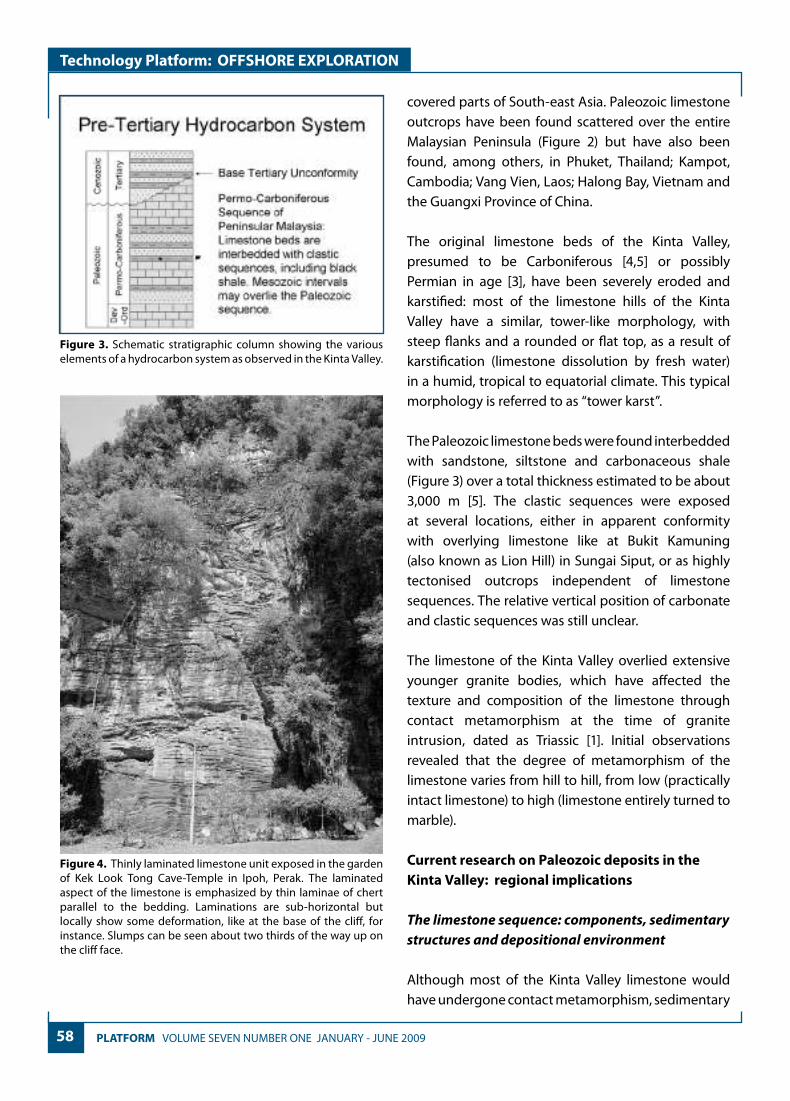
58 PLATFORM VOLUME SEVEN NUMBER ONE JANUARY - JUNE 2009
Technology Platform: OFFSHORE EXPLORATION
covered parts of South-east Asia. Paleozoic limestone outcrops have been found scattered over the entire Malaysian Peninsula (Figure 2) but have also been found, among others, in Phuket, Thailand; Kampot, Cambodia; Vang Vien, Laos; Halong Bay, Vietnam and the Guangxi Province of China.
The original limestone beds of the Kinta Valley, presumed to be Carboniferous [4,5] or possibly Permian in age [3], have been severely eroded and karstified: most of the limestone hills of the Kinta Valley have a similar, tower-like morphology, with steep flanks and a rounded or flat top, as a result of karstification (limestone dissolution by fresh water) in a humid, tropical to equatorial climate. This typical morphology is referred to as “tower karst”.
The Paleozoic limestone beds were found interbedded with sandstone, siltstone and carbonaceous shale (Figure 3) over a total thickness estimated to be about 3,000 m [5]. The clastic sequences were exposed at several locations, either in apparent conformity with overlying limestone like at Bukit Kamuning (also known as Lion Hill) in Sungai Siput, or as highly tectonised outcrops independent of limestone sequences. The relative vertical position of carbonate and clastic sequences was still unclear.
The limestone of the Kinta Valley overlied extensive younger granite bodies, which have affected the texture and composition of the limestone through contact metamorphism at the time of granite intrusion, dated as Triassic [1]. Initial observations revealed that the degree of metamorphism of the limestone varies from hill to hill, from low (practically intact limestone) to high (limestone entirely turned to marble).
Current research on Paleozoic deposits in the Kinta Valley: regional implications
The limestone sequence: components, sedimentary structures and depositional environment
Although most of the Kinta Valley limestone would have undergone contact metamorphism, sedimentary
Figure 4. Thinly laminated limestone unit exposed in the garden of Kek Look Tong Cave-Temple in Ipoh, Perak. The laminated aspect of the limestone is emphasized by thin laminae of chert parallel to the bedding. Laminations are sub-horizontal but locally show some deformation, like at the base of the cliff, for instance. Slumps can be seen about two thirds of the way up on the cliff face.
Figure 3. Schematic stratigraphic column showing the various elements of a hydrocarbon system as observed in the Kinta Valley.

59 VOLUME SEVEN NUMBER ONE JANUARY - JUNE 2009 PLATFORM
Technology Platform: OFFSHORE EXPLORATION
structures were observed and, in places, components of the rock could be identified. The less metamorphosed limestone of Chemor and the practically intact black limestone of Sungai Siput, in the northern part of the Kinta Valley, allowed full identification of the rock components and sedimentary structures.
The limestone exposed in the Kinta Valley was, for the most part, seen as thinly-bedded to laminated micritic limestone with thin interbedded chert laminations (Figure 4). It had no apparent matrix porosity or permeability. The thinly-bedded limestone seemed locally deformed displaying double folds in the shape of an “S”, ranging in vertical size from several centimetres to 5 or more metres (Figure 4). This study interpreted these folds as slumps, syn-sedimentary folding which could have resulted from plastic/ductile deformation of soft but cohesive sediment packages due to gravity-induced lateral downwards movement, usually on a slope. In the Kinta Valley, where slump structures are common in the Paleozoic limestone, individual S-shaped slumps were generally sandwiched between relatively undisturbed layers of thinly-bedded to laminated limestone (Figure 4).
The thinly-bedded sequence was interpreted to be a deep marine slope deposit, where the slope had a gradient high enough to allow the slumping observed at outcrops. The common occurrence of chert layers and chert laminae further suggested that the limestone was deposited in relatively deep water.
Thicker beds of limestone (0.5 to 2 m thick) occasionally interrupted the monotonous thinly bedded limestone sequence (Figure 5). These thicker beds were made up of coarser carbonate components and consisted of either crinoid packstone to wackestone (Figure 6), bioclastic packstone to grainstone or breccia. The breccia beds comprised sub-rounded blocks, 2 cm to 50 cm in size, mainly made up of shallow-marine limestone (Figure 7). These beds were interpreted as base-of-slope breccias, re-deposited grainstones (mass-flows) or turbidites.
Observations and interpretations of sedimentary structures and rock components in the limestone
Figure 5. A series of thicker beds, up to 2 m thick, within a sequence of thinly-bedded limestone in Chemor, Perak. The thinly-bedded unit represents deep marine lower slope deposits whereas the thicker beds, composed of shallow-marine skeletal grainstone, packstone and breccias, are redeposited as turbidites and debris-flows on the lower slope
Figure 7. A thick bed exposed in Chemor, Perak is a re-deposited breccia bed containing a block of shallow marine limestone rich in brachiopods and algae, about 40 cm in diameter, along with smaller breccia blocks incorporated in a fine micritic matrix.
Figure 6. Some of the thicker beds consist of crinoidal packstone to wackestone, as on this photograph. The crinoid stem fragments are incorporated in a micritic matrix that seems to be laminated. Field of view is approximately 10 cm (Photograph by Cheang Kum Seng).
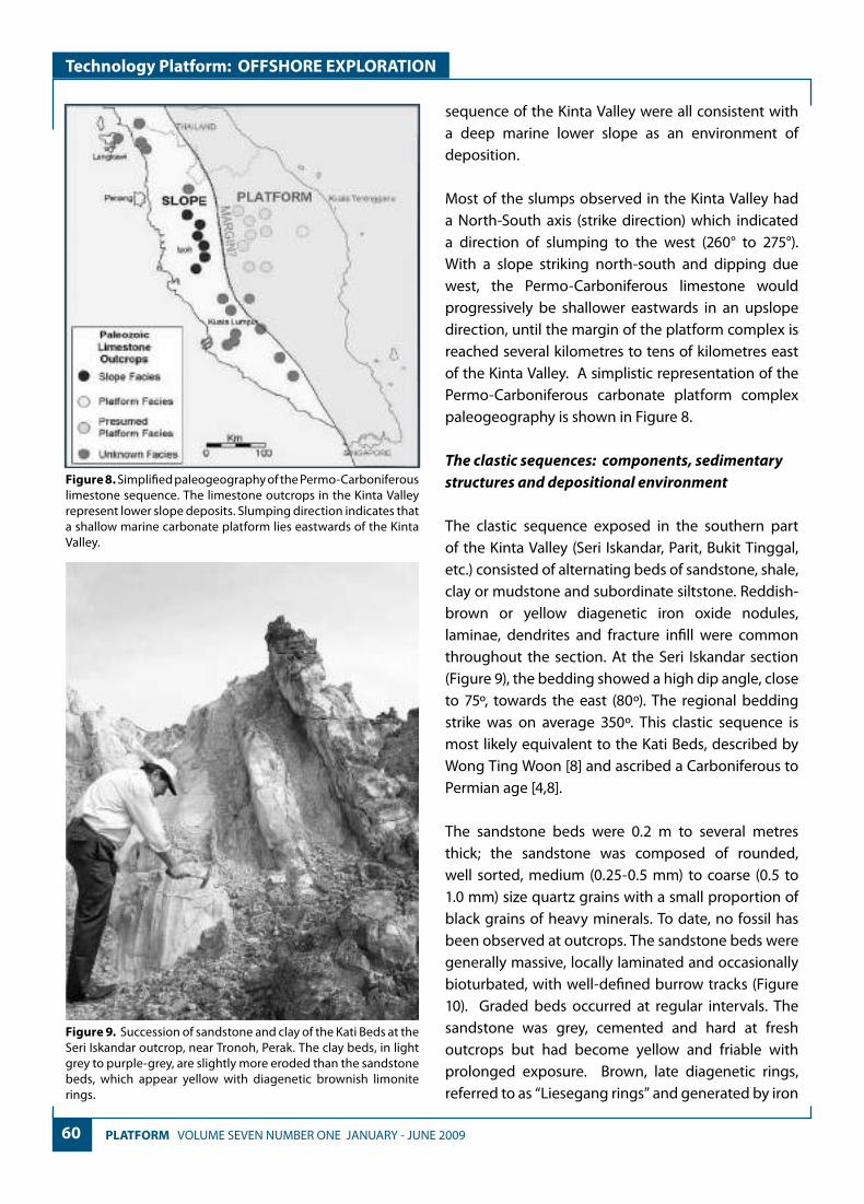
60 PLATFORM VOLUME SEVEN NUMBER ONE JANUARY - JUNE 2009
Technology Platform: OFFSHORE EXPLORATION
sequence of the Kinta Valley were all consistent with a deep marine lower slope as an environment of deposition.
Most of the slumps observed in the Kinta Valley had a North-South axis (strike direction) which indicated a direction of slumping to the west (260° to 275°). With a slope striking north-south and dipping due west, the Permo-Carboniferous limestone would progressively be shallower eastwards in an upslope direction, until the margin of the platform complex is reached several kilometres to tens of kilometres east of the Kinta Valley. A simplistic representation of the Permo-Carboniferous carbonate platform complex paleogeography is shown in Figure 8.
The clastic sequences: components, sedimentary structures and depositional environment
The clastic sequence exposed in the southern part of the Kinta Valley (Seri Iskandar, Parit, Bukit Tinggal, etc.) consisted of alternating beds of sandstone, shale, clay or mudstone and subordinate siltstone. Reddish-brown or yellow diagenetic iron oxide nodules, laminae, dendrites and fracture infill were common throughout the section. At the Seri Iskandar section (Figure 9), the bedding showed a high dip angle, close to 75º, towards the east (80º). The regional bedding strike was on average 350º. This clastic sequence is most likely equivalent to the Kati Beds, described by Wong Ting Woon [8] and ascribed a Carboniferous to Permian age [4,8].
The sandstone beds were 0.2 m to several metres thick; the sandstone was composed of rounded, well sorted, medium (0.25-0.5 mm) to coarse (0.5 to 1.0 mm) size quartz grains with a small proportion of black grains of heavy minerals. To date, no fossil has been observed at outcrops. The sandstone beds were generally massive, locally laminated and occasionally bioturbated, with well-defined burrow tracks (Figure 10). Graded beds occurred at regular intervals. The sandstone was grey, cemented and hard at fresh outcrops but had become yellow and friable with prolonged exposure. Brown, late diagenetic rings, referred to as “Liesegang rings” and generated by iron
Figure 8. Simplified paleogeography of the Permo-Carboniferous limestone sequence. The limestone outcrops in the Kinta Valley represent lower slope deposits. Slumping direction indicates that a shallow marine carbonate platform lies eastwards of the Kinta Valley.
Figure 9. Succession of sandstone and clay of the Kati Beds at the Seri Iskandar outcrop, near Tronoh, Perak. The clay beds, in light grey to purple-grey, are slightly more eroded than the sandstone beds, which appear yellow with diagenetic brownish limonite rings.

61 VOLUME SEVEN NUMBER ONE JANUARY - JUNE 2009 PLATFORM
Technology Platform: OFFSHORE EXPLORATION
oxide staining, were present in almost all sandstone layers.
Siltstone beds were mainly quartzitic and locally displayed grading into fine sandstone. Some siltstone beds contained a proportion of clay. Diagenetic features similar to those observed in sandstone beds were common in siltstone layers.
Clay occurred as beds, a few centimetres to several metres thick, interbedded with sandstone and siltstone layers (Figure 11). Contacts between clay beds and coarser beds were usually sharp and were commonly enhanced by erosion at the outcrop. The clay beds were light grey to greyish purple in colour. Diagenetic reddish-purple streaks, sub-parallel and sub-perpendicular to the bedding plane, were ubiquitous throughout the clay beds (Figure 11). The clay was hard but friable when dry but would become soft and ductile when wet. Traces of plant fragments were found in some clay beds. The nature, origin and age of the plant remains, however, were not determined.
The clastic beds were locally folded and contained slumps, load structures and flame structures. Flute casts were reported by Wong Ting Woon [9]. These sedimentary structures indicated episodic rapid deposition of the coarser beds and, together with the slump structures, suggested deposition as turbiditic beds on the lower part of a marine slope.
The clastic sequence that underlied the limestone at Bukit Kamuning in Sungai Siput predominantly consisted of thinly laminated siltstone, shale and some sandstone beds, with local chert-rich beds. A layer of black shale, several metres thick, was visible at the base of the section.
Apart from the Bukit Kamuning section in Sungai Siput, where the clastic sequence was clearly underlying limestone beds, the relationship between the clastic and carbonate sequences was unclear. Even in Sungai Siput, however, it was not certain whether the limestone sequence lied conformably above the clastic sequence. The sedimentary structures and
Figure 10. Burrow tracks in a sandstone layer of the Kati Beds at the Seri Iskandar outcrop, near Tronoh, Perak. The diagenetic coloration in purple highlights the burrow tracks. The burrow tubes are approximately 5 mm in diameter and are regularly spaced within this 1.5 m thick sandstone layer.
Figure 11. A 60 cm-thick clay bed is interbedded with sandstone layers at the Seri Iskandar outcrop, near Tronoh, Perak. The contact between clay and sandstone beds is very sharp. The grey clay bed contains numerous thin diagenetic purple layers parallel and perpendicular to the bedding plane.

62 PLATFORM VOLUME SEVEN NUMBER ONE JANUARY - JUNE 2009
Technology Platform: OFFSHORE EXPLORATION
rock components indicated that both carbonate and clastic sequences were deposited in a relatively deep marine slope environment. Could the clastic sequence exposed in the Kinta Valley represent a lowstand wedge? If so, its presence would be mostly confined to the slope and basin in the western part of Peninsular Malaysia. If Paleozoic clastic sediments, time-equivalent to the lowstand wedge, were deposited over the carbonate platform areas in the eastern part of Peninsular Malaysia and in the Malay Basin, it would most likely have consisted of fluvial or continental deposits. Ongoing research at UTP on the carbonate and clastic sequences would address issues related to the age, relative position and lateral extent of the various Paleozoic sequences.
Elements of a Paleozoic Hydrocarbon System: Observations and Discussion
Source Rocks
Several layers of black carbonaceous shale, rich in organic matter were part of the clastic sequences and
could constitute potential source rocks. Thick intervals of black shale (up to 10 m thick) were exposed at several locations near Batu Gajah (Figure 12) and along the new road leading to Gopeng. This black shale may have been part of or equivalent to the “Kim Loong No. 3 Beds” of Suntharalingam [6]. Samples collected at one of these outcrops had a measured Total Organic Content (TOC) greater than 6% (Mohamed Jamaal Hoesni, Pers. Com.), which meant a very good source rock. The TOC value would be even higher if it were corrected to its original pre-maturation value. These source rock layers could, however, have reached maturity at an early stage, possibly even in the Triassic, at the time of emplacement of granitic intrusions, before traps were formed.
Layers of black shale, 2 to 4 metres thick, were also found at the base of the clastic sequence at Bukit Kamuning in Sungai Siput. This sequence seemed to have suffered little from contact metamorphism and may have matured at a later, more opportune time. Samples from this black shale outcrop have not been measured yet for TOC.
Figure 12. A thick layer of black carbonaceous shale outcrops near Batu Gajah, Perak. This layer is more than 10 m thick. The shale is slightly metamorphosed but still contains organic matter. A measured TOC (Total Organic Content) of 6% makes this a good potential source rock.

63 VOLUME SEVEN NUMBER ONE JANUARY - JUNE 2009 PLATFORM
Technology Platform: OFFSHORE EXPLORATION
Black calcareous shale layers were also found within the limestone sequence. Several of these layers, 5 to 10 cm thick each, interbedded with chert layers of a similar thickness are part of a complex series of slumps exposed at an abandoned black limestone quarry in Sungai Siput (Figure 13).
These three occurrences of black shale were associated with carbonate or clastic sequences presumed to be of Permo-Carboniferous age and were therefore thought to be of a similar age. Were these potential marine source rocks laterally continuous eastwards? Probably not if they were part of a deep marine or slope sequence, unless similar deep marine conditions existed to the east of Peninsular Malaysia, for instance. Yet, a number of black shale intervals, possibly Triassic, Permian or older, have been reported from several sites on Peninsular Malaysia. Permo-Carboniferous source rocks possibly reached maturity at an early stage in the area of the Peninsula but could have
matured at an opportune time offshore, in the Malay Basin for instance.
Reservoirs
Carbonate and clastic sequences could have contained potential reservoir intervals, either as sandstone layers or shallow marine limestones. Although the carbonate sequence of the Kinta Valley, mainly composed of micritic slope deposits, contained no potential reservoir, its analysis led to a schematic palaeogeographic reconstruction of the Permo-Carboniferous carbonate platform complex suggesting that reservoir lithologies in the form of shallow marine carbonates could be found in the eastern part and off the eastern coast of Peninsular Malaysia.
Outcrops in eastern Peninsular Malaysia confirmed the presence of a shallow marine Paleozoic platform complex, with potential reservoir horizons, that
Figure 13. Part of a complex slump exposed in an abandoned black limestone quarry at Sungai Siput, Perak. The layers involved in the slump include chert (in light grey), micritic limestone (medium grey) and carbonaceous shale (dark grey).
64 PLATFORM VOLUME SEVEN NUMBER ONE JANUARY - JUNE 2009
Technology Platform: OFFSHORE EXPLORATION
probably extended eastwards, far into the China Sea. In the early 1970s, pre-Tertiary carbonate have penetrated offshore, at three localities in the southern part of the Malay Basin. These wells found from 8 to 492 m of limestone, interpreted to be Triassic [3] below the Base Tertiary unconformity. The reservoir quality of these deposits was uncertain.
Clastic sequences comprising sandstone layers could form potentially good reservoirs. The sandstone beds exposed at Seri Iskandar made up more than 50% of the entire exposed sequence and their total thickness probably exceeded 400 metres. The lateral extent of these deposits was unknown. Should the clastic sequence represent a lowstand wedge, it would mostly be confined to the western part of Peninsular Malaysia, where valid hydrocarbon plays would very unlikely to be found, in view of the shallowness or exposed state of the reservoirs. It was, therefore, uncertain whether these sandstones or a time-equivalent clastic sequence ever extended to where the carbonate platforms developed and whether it could be found in the subsurface in the eastern part of the Peninsula or offshore, east of the peninsula.
Seals
Clay and shale layers within the clastic sequences could act as intraformational seals, providing reservoir-seal pairs within the clastic sequences. Should clastic sequences extend over the Paleozoic carbonate platform areas to the east of the Peninsula, they could provide regional seals above carbonate sequences.
The existence of sealing lithologies within the carbonate sequences was unknown but effective seals within carbonate platform sequences are rare. The Paleozoic carbonate sequences could, however, be covered by Paleozoic or younger (Mesozoic) sealing lithologies in the Malay Basin but this remained, so far, rather speculative. It was also found possible that the Base Tertiary unconformity could have regional sealing capacity. Oligocene shale, for instance, was found overlying pre-Tertiary limestone basement rock in a well drilled in the southern part of the Malay Basin [2].
Traps
The wells drilled below the Base Tertiary unconformity east of Peninsular Malaysia did not encounter hydrocarbons. It could be likely that these wells were drilled to test Tertiary structures but Paleozoic structures could be offset from the Tertiary structures at these locations. Tertiary deposits lied unconformably above pre-Tertiary sequences, which have undergone considerable structural deformation prior to deposition and folding of Tertiary deposits. Paleozoic structures would therefore be, to a large extent, independent from younger Tertiary structures.
Structural and possibly stratigraphic traps and even “buried hills” traps, so far untested, probably exist east of Peninsular Malaysia and in the Malay Basin. The existing 2D seismic coverage of the Malay Basin provided hints of pre-Tertiary structures but an unambiguous identification of these potential traps was, unfortunately, hampered by the poor seismic imaging below the Base Tertiary unconformity.
CONCLUSIONS
The presence of an effective hydrocarbon system in Paleozoic deposits of Peninsular Malaysia and in the Malay Basin was still speculative but was not ruled out. Initial results in the investigation of Paleozoic carbonate and clastic sequences outcropping in the Kinta Valley, Peninsular Malaysia, provided encouraging indications for the existence of source rocks, reservoirs and seals but many pieces of the puzzle were still missing.
If they existed, Paleozoic hydrocarbon plays have a better chance of being found east of Peninsular Malaysia, in the western part of the Malay Basin.
Good Paleozoic source rocks and potential source rock horizons were found in the western part of Peninsular Malaysia. Whether these source rocks extended to the east of the Peninsula and offshore, in the Malay Basin, was still uncertain. The timing of maturation and hydrocarbon generation of these potential source rocks may have been too early to effectively charge

65 VOLUME SEVEN NUMBER ONE JANUARY - JUNE 2009 PLATFORM
Technology Platform: OFFSHORE EXPLORATION
Paleozoic traps. Charge risk was therefore considered high.
Initial results of investigations into Paleozoic carbonates suggested the presence of favourable potential reservoir lithologies in the eastern part of Peninsular Malaysia and offshore in the Malay Basin. The quality of the potential carbonate reservoirs was not known. The presence of clastic reservoirs in these areas remained speculative. Reservoir risk was therefore qualified as medium.
Sealing lithologies were found in the Paleozoic clastic sequences of the Kinta Valley. It was, however, uncertain whether these clastic sequences extended eastwards into the Malay Basin. Paleozoic or younger shale beds as well as lithologies associated with the pre-Tertiary unconformity may act as effective seals to the east but because of the speculative nature of the existence of these lithologies, seal risk was considered medium to high.
The complex structural history of pre-Tertiary deposits on or near Peninsular Malaysia may likely have generated structural traps. Stratigraphic traps may have existed below the Base Tertiary unconformity. Resolving the seismic imaging issue in pre-Tertiary deposits could help identify untested Paleozoic structures or even “buried hills” east of Peninsular Malaysia.
Further studies are needed in order to reduce the many uncertainties currently inherent to potential Paleozoic plays east of Peninsular Malaysia. The ongoing investigations carried out at UTP could be focused on providing answers to the many remaining questions.
References
[1] Cobbing, E.J., P.E.J. Pitfield, D.P.F. Darbyshire, and D.I.J. Mallick, 1992. The granites of the South-East Asian tin belt, Overseas Memoir 10, British Geological Survey, London, p. 79-86
[2] Fontaine, H., Rodziah Daud and Singh Updesh, 1990. A Triassic “reefal” limestone in the basement of the Malay Basin, South China Sea: regional implications. Geol. Soc. Malaysia Bulletin Vol. 27, p. 1-25.
[3] Fontaine, H. and Ibrahim Bin Amnan, 1995. Biostratigraphy of the Kinta Valley, Perak. Geol. Soc. Malaysia Bulletin, Vol. 38, p. 159-172
[4] Hutchison, C.S., 2007. Geological Evolution of South-East Asia (2nd Edition), Geological Society of Malaysia (Publ), 433 p.
[5] Ingham, F.T. and E.P. Bradford, 1960. The geology and mineral resources of the Kinta Valley, Perak. Geological Survey District Memoir 9, Federation of Malaya Geological Survey, Ipoh, 347 p.
[6] Suntharalingam, T., 1968. Upper Paleozoic stratigraphy of the area west of Kampar, Perak. Geol. Soc. Malaysia Bulletin, Vol. 1, p. 1-15.
[7] Tjia, H.D., 1999. Pre-Tertiary Hydrocarbon Potential. In: Leong Khee Meng (Editor) The Petroleum Geology and Resources of Malaysia, Published by Petroliam Nasional Berhad (PETRONAS), Chapter 26, p. 605-635.
[8] Wong Ting Woon, 1991. Geology and mineral resources of the Lumut-Teluk Intan area, Perak Darul Ridzuan. Geological Survey of Malaysia Map Report 3, 96 p. Published by the Geological Survey Laboratory, Ipoh, Perak.
Born in Belgium in 1949, Professor Dr Bernard Pierson received his Bachelor’s degree in Geology and Mineralogy from the Université Catholique de Louvain, Belgium in 1973. He moved to the US for post-graduate studies and was awarded the MSc in Geology by the University of Kentucky in 1976 and a PhD in Marine Geology and Geophysics from the
University of Miami (Rosenstiel School for Marine & Atmospheric Sciences) in 1980; specialising in carbonate sedimentology and petrography. He joined Shell in 1980 as a Research Geologist with the carbonate team at Shell Research in Rijswijk, the Netherlands. His Shell career took him to The Netherlands, Oman, Argentina, Colombia, Pakistan and Abu Dhabi. In March 2007, he joined Universiti Teknologi PETRONAS (UTP), in Tronoh, Malaysia as the Shell Chair in Petroleum Geosciences. He supervises 6 post-graduate students and teaches geology and carbonate sedimentology in the undergraduate and post-graduate programmes of UTP. Professor Pierson is married and lives in Ipoh, Perak, Malaysia with his wife. He has two children who live and work in Belgium.

66 PLATFORM VOLUME SEVEN NUMBER ONE JANUARY - JUNE 2009
Technology Platform: RESERVOIR ENGINEERING
INTRODUCTION
Free convection flows past a vertical surface or plate were studied extensively in the literature due to its applications in engineering and environmental processes. Several investigations were performed using both analytical and numerical methods under different thermal conditions which are continuous and well-defined at the wall. Practical problems often involve wall conditions that are non-uniform or arbitrary. To understand such problems, it is useful to investigate problems subject to step change in wall temperature. Keeping this in view, Schetz [1] made an attempt to develop an approximate analytical model for free convection flow from a vertical plate with discontinuous wall temperature conditions. Several investigations were continued on this problem using
an experimental technique [2], numerical methods [3], and by using series expansions [4, 5]. Lee and Yovanovich [6] presented a new analytical model for the laminar natural convection from a vertical plate with step change in wall temperature. The validity and accuracy of the model is demonstrated by comparing with the existing results. Chandran et al. [7] have presented an analytical solution to the unsteady natural convection flow of an incompressible viscous fluid near a vertical plate with ramped wall temperature and they have compared the results with constant temperature. Recently, Saha et al. [8] investigated the natural convection boundary layer adjacent to an inclined semi-infinite flat plate subjected to ramp heating. The flow development from the start-up to an eventual steady state has been described based on scaling analysis and verified by numerical simulations.
EFFECTS OF MASS TRANSFER AND FREE CONVECTION CURRENTS ON THE FLOW PAST AN INFINITE VERTICAL
PLATE WITH RAMPED WALL TEMPERATURE
Narahari Marneni* and O. Anwar Bég***Universiti Teknologi PETRONAS, 31750 Tronoh, Perak Darul Ridzuan, Malaysia **Sheffield Hallam University, Sheffield, South Yorkshire, S1 1WB, England, UK
*[email protected] and **[email protected]
ABSTRACT
An exact analysis of the flow of an incompressible viscous fluid past an infinite vertical plate is carried out on taking into account the presence of foreign mass or constant mass flux and ramped wall temperature. The dimensionless governing coupled linear partial differential equations are solved using the Laplace transform technique. Two different solutions for the fluid velocity are obtained – one valid for the fluids of Schmidt numbers different from unity, and the other for which the Schmidt number is unity. The effects of different parameters like Prandtl number (Pr), Schmidt number (Sc), time (t) and mass to thermal buoyancy ratio parameter (N ) for both aiding and opposing buoyancy effects on the velocity and skin-friction are studied. Also, the heat and mass transfer effects on the flow near a ramped temperature plate has been compared with the flow near a plate with constant temperature.
Keywords: vertical plate, natural convection, ramped wall temperature, heat and mass transfer.
This paper was presented at the 5th Asian Methematical Conference, Kuala Lumpur, 22-26 June 2009

67 VOLUME SEVEN NUMBER ONE JANUARY - JUNE 2009 PLATFORM
Technology Platform: RESERVOIR ENGINEERING
Free convection flows occur not only due temperature difference, but also due to concentration difference or the combination of these two. The study of combined heat and mass transfer play an important role in the design of chemical processing equipment, nuclear reactors, formation and dispersion of fog etc. The effect of presence of foreign mass on the free convection flow past a semi-infinite vertical plate was first studied by Gebhart and Pera [9]. Soundalgekar [10] has studied mass transfer effects on flow past an impulsively started infinite isothermal vertical plate. Dass et al. [11] considered the mass transfer effects on flow past an impulsively started infinite isothermal vertical plate with constant mass flux. Muthucumaraswamy et al. [12] presented an exact solution to the problem of flow past an impulsively started infinite vertical plate in the presence of uniform heat and mass flux at the plate using Laplace transform technique.
However, mass transfer effects on free convection flow past an infinite vertical plate subject to discontinuous or non-uniform wall temperature conditions have not been studied in the literature. Hence, it is proposed to study the effects of mass transfer on the free convection flow of an incompressible viscous fluid past an infinite vertical plate subject to ramped wall temperature in case of (i) foreign mass and (ii) constant mass flux at the plate. In section 2 the mathematical analysis is presented, exact solutions to the non-dimensional coupled linear partial differential equations were derived by the Laplace transform method and in section 3, the conclusions are set out.
MATHEMATICAL ANALYSIS
Consider the flow of a viscous incompressible fluid past an infinite vertical plate. The x′ - axis is taken along the plate in the vertically upward direction, and the y′ - axis is taken normal to the plate. Initially, for time 0≤′t , both the plate and the fluid are assumed to be at the same temperature ∞′T and concentration
∞′C . At time 0>′t , the temperature of the plate is raised or lowered to
0/)( ttTTT w ′′−′+′ ∞∞ when
0tt ≤′ , and thereafter, for 0tt >′ , is maintained at the constant temperature wT ′ and the concentration level at the plate is raised to wC′ or concentration is
supplied at a constant rate to the plate. Then under usual Boussinesq’s approximation, the unsteady flow past an infinite vertical plate is governed by the following equations [10-12]:
2
2* )()(
y
uCCgTTg
t
u
′∂′∂+′−′+′−′=
′∂′∂
∞∞ νββ (1)
2
2
y
Tk
t
TCp ′∂
′∂=′∂′∂ρ (2)
2
2
y
CD
t
C
′∂′∂=
′∂′∂
(3)
With the following initial and boundary conditions:
∞→′′→′′→′→′
=′′′−=
′∂′∂′=′
=′
>′′
≤′<′′−′+′
=′
=′=′
>′
≥′′=′′=′=′≤′
∞∞
∞∞
∞∞
.as,,0
0ator
0at
for
0for)(
0at0
:0
,0for,,0:0
0
00
yCCTTu
yD
j
y
CCC
y
ttT
ttt
tTTT
T
yu
t
yCCTTut
w
w
w (4)
As the plate is assumed to be infinite in length in the −′x direction, hence all the physical variables are functions of y′ and t ′ only. Here u′ is the velocity in the −′x direction, t ′ the time, g the acceleration due to gravity, β the volumetric coefficient of thermal expansion, *β the volumetric coefficient of expansion for concentration, T ′ the temperature of the fluid near the plate, ∞′T the temperature of the fluid far away from the plate, C′ the species concentration near the plate,
∞′C the species concentration in the fluid far away from the plate, wT ′ the plate temperature, wC′ the species concentration at the plate, 0t the characteristic time, ν the kinematic viscosity, ρ the density, pC the specific heat at constant pressure, k the thermal conductivity of the fluid, j ′′ the mass flux per unit area at the plate and D is the mass diffusion coefficient.
On introducing the following non-dimensional quantities:
(5)
=′′
=′−′
=
=
′′′−′
=′−′′−′
=′−′
=
=′−′′−′
=′
=′−′
′=
′=
′=
∞
∞
∞
∞∞
∞
∞
∞
.,or)(
,Sc,or,)(
,Pr,,Gr)(
,,
20
*2/30
*
0
2/30
0
000
Gr
GmN
D
tjgGm
tCCgGm
D
D
tj
CCC
CC
CCC
tTTgGr
k
C
TT
TTtu
TTgt
uu
t
tt
t
yy
w
w
w
p
ww
βν
β
ννν
β
µθ
νβν

68 PLATFORM VOLUME SEVEN NUMBER ONE JANUARY - JUNE 2009
Technology Platform: RESERVOIR ENGINEERING
In Eqs. (1) – (4), leads to
2
2
y
uNC
t
u
∂∂++=
∂∂ θ (6)
2
2
Pryt ∂
∂=∂∂ θθ
(7)
2
2
Scy
C
t
C
∂∂=
∂∂
(8)
Where u the dimensionless velocity, y the dimensionless coordinate axis normal to the plate, t the dimensionless time, θ the dimensionless temperature, C the dimensionless concentration, Gr thermal Grashof number, Gm mass Grashof number, Pr the Prandtl number, µ the coefficient of viscosity, Sc the Schmidt number, and N is the buoyancy ratio parameter. According to the above non-dimensionalisation process, the characteristic time 0t can be defined as
3/2
0 )(
′−′
=∞TTg
twβν
(9)
The corresponding initial and boundary conditions in dimensionless form are:
∞→→→→
==∂∂=
>≤<
==>
≥===≤
.as0,0,0
,0at-1or1,1for1
10for,0:0
,0for0,0,0:0
yCu
yy
CC
t
ttut
yCut
θ
θ
θ
(10)
These equations (6) – (8) are coupled linear system of partial differential equations, which can be solved by the usual Laplace transform technique subject to the initial and boundary conditions (10). Then the solutions are:
Case I: 1Sc,1Pr ≠≠
(Foreign mass) (11a)
),Sc(Sc
1),( 3 tyFtyC =
(Constant mass flux) (11b)
)1()1,Pr(),Pr(),( 11 −−−= tHtyFtyFtyθ
(12)
[
[ ]),Sc(),(1)-(Sc
)1()1,(),()1(Pr
1),(
11
22
tyFtyFN
tHtyFtyFtyu
−+
])1()1,Pr(),Pr( 22 tHtyFtyF −−+−
−−−−
=
(Foreign mass) (13a)
),( tyu
[ ]),Sc(),(1)-(ScSc
44 tyFtyFN −+
])1()1,Pr(),Pr( 22 tHtyFtyF −−+−
[ )1()1,(),()1(Pr
122 tHtyFtyF −−−
−=
(Constant mass flux) (13b)
Case II: 1Sc,1Pr =≠
[
]
),(2
)1()1,Pr(),Pr(
)1()1,(),()1(Pr
1),(
3
22
22
tyyFN
tHtyFtyF
tHtyFtyFtyu
+
−−+−
−−−−
=
(Foreign mass) (13c)
(Constant mass flux) (13d)
where
−−
+=
t
ztz
t
zt
ztzF
4exp)/(
2erfc
2),(
22
1 π
=
t
ytyC
2
Scerfc),(
[
]
),(2
)1()1,Pr(),Pr(
)1()1,(),()1(Pr
1),(
1
22
22
tyyFN
tHtyFtyF
tHtyFtyFtyu
+
−−+−
−−−−
=
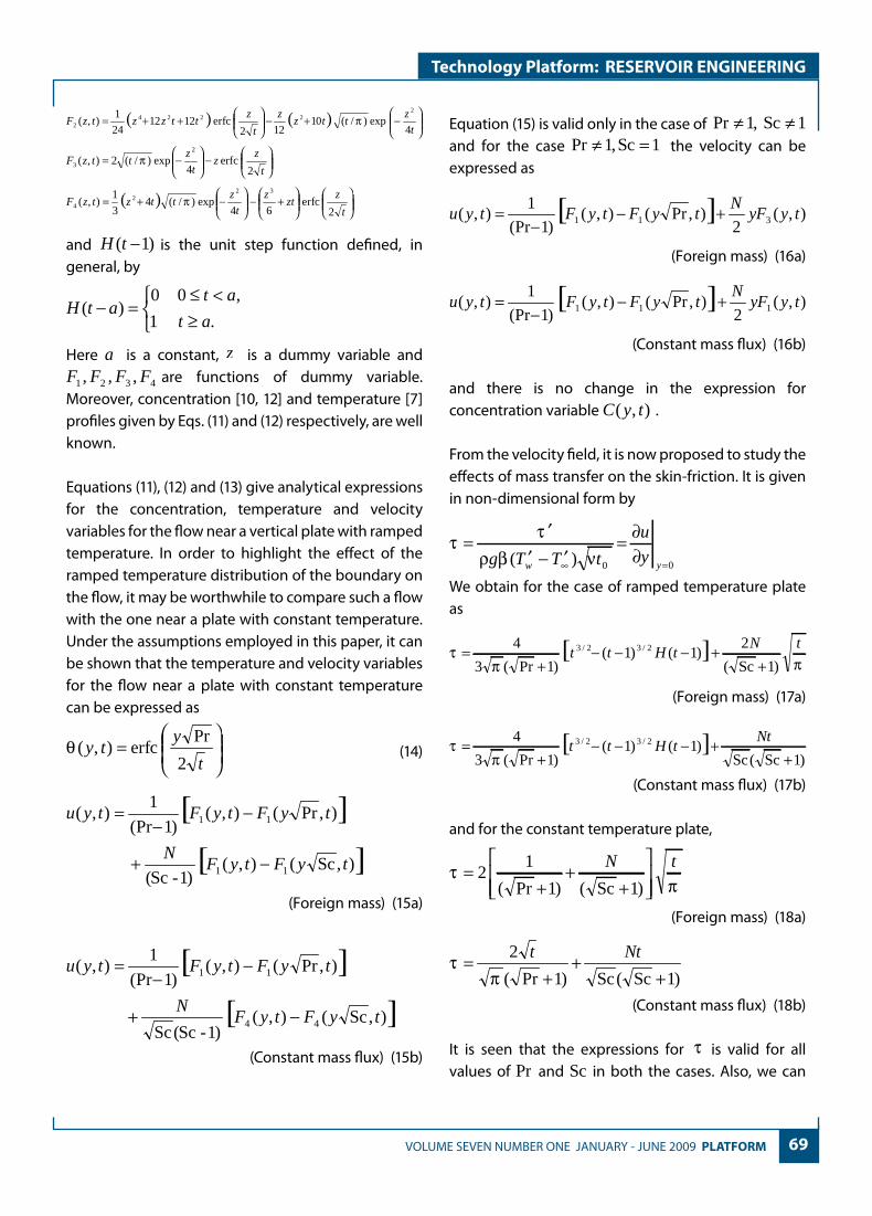
69 VOLUME SEVEN NUMBER ONE JANUARY - JUNE 2009 PLATFORM
Technology Platform: RESERVOIR ENGINEERING
−
−=
t
zz
t
zttzF
2erfc
4exp)/(2),(
2
3 π
( )
+−
−+=
t
zzt
z
t
zttztzF
2erfc
64exp)/(4
3
1),(
322
4 π
and )1( −tH is the unit step function defined, in general, by
≥<≤
=−.1
,00)(
at
atatH
Here a is a constant, z is a dummy variable and
4321 ,,, FFFF are functions of dummy variable. Moreover, concentration [10, 12] and temperature [7] profiles given by Eqs. (11) and (12) respectively, are well known.
Equations (11), (12) and (13) give analytical expressions for the concentration, temperature and velocity variables for the flow near a vertical plate with ramped temperature. In order to highlight the effect of the ramped temperature distribution of the boundary on the flow, it may be worthwhile to compare such a flow with the one near a plate with constant temperature. Under the assumptions employed in this paper, it can be shown that the temperature and velocity variables for the flow near a plate with constant temperature can be expressed as
=
t
yty
2
Prerfc),(θ (14)
(Foreign mass) (15a)
[ ][ ]),Sc(),(
1)-(ScSc
),Pr(),()1(Pr
1),(
44
11
tyFtyFN
tyFtyFtyu
−+
−−
=
(Constant mass flux) (15b)
Equation (15) is valid only in the case of 1Sc,1Pr ≠≠ and for the case 1Sc,1Pr =≠ the velocity can be expressed as
[ ] ),(2
),Pr(),()1(Pr
1),( 311 tyyF
NtyFtyFtyu +−
−=
(Foreign mass) (16a)
[ ] ),(2
),Pr(),()1(Pr
1),( 111 tyyF
NtyFtyFtyu +−
−=
(Constant mass flux) (16b)
and there is no change in the expression for concentration variable ),( tyC .
From the velocity field, it is now proposed to study the effects of mass transfer on the skin-friction. It is given in non-dimensional form by
00)( =∞ ∂∂=
′−′′
=yw
y
u
tTTg νβρττ
We obtain for the case of ramped temperature plate as
[ ]ππ
τ tNtHtt
)1Sc(
2)1()1(
)1Pr(3
4 2/32/3
++−−−
+=
(Foreign mass) (17a)
[ ])1Sc(Sc
)1()1()1Pr(3
4 2/32/3
++−−−
+= Nt
tHttπ
τ
(Constant mass flux) (17b)
and for the constant temperature plate,
πτ tN
++
+=
)1Sc()1Pr(
12
(Foreign mass) (18a)
)1Sc(Sc)1Pr(
2
++
+= Ntt
πτ
(Constant mass flux) (18b)
It is seen that the expressions for τ is valid for all values of Pr and Sc in both the cases. Also, we can
( ) ( )
−+−
++=
t
zttz
z
t
zttzztzF
4exp)/(10
122erfc1212
24
1),(
22224
2 π
[ ][ ]),Sc(),(
1)-(Sc
),Pr(),()1(Pr
1),(
11
11
tyFtyFN
tyFtyFtyu
−+
−−
=
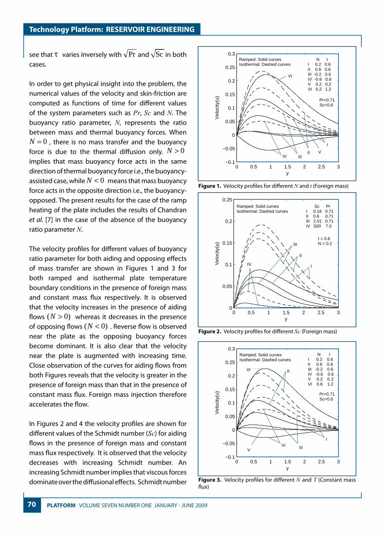
70 PLATFORM VOLUME SEVEN NUMBER ONE JANUARY - JUNE 2009
Technology Platform: RESERVOIR ENGINEERING
see that τ varies inversely with Pr and Sc in both cases.
In order to get physical insight into the problem, the numerical values of the velocity and skin-friction are computed as functions of time for different values of the system parameters such as Pr, Sc and N. The buoyancy ratio parameter, N, represents the ratio between mass and thermal buoyancy forces. When
0=N , there is no mass transfer and the buoyancy force is due to the thermal diffusion only. 0>N implies that mass buoyancy force acts in the same direction of thermal buoyancy force i.e., the buoyancy-assisted case, while 0<N means that mass buoyancy force acts in the opposite direction i.e., the buoyancy-opposed. The present results for the case of the ramp heating of the plate includes the results of Chandran et al. [7] in the case of the absence of the buoyancy ratio parameter N.
The velocity profiles for different values of buoyancy ratio parameter for both aiding and opposing effects of mass transfer are shown in Figures 1 and 3 for both ramped and isothermal plate temperature boundary conditions in the presence of foreign mass and constant mass flux respectively. It is observed that the velocity increases in the presence of aiding flows )0( >N whereas it decreases in the presence of opposing flows )0( <N . Reverse flow is observed near the plate as the opposing buoyancy forces become dominant. It is also clear that the velocity near the plate is augmented with increasing time. Close observation of the curves for aiding flows from both Figures reveals that the velocity is greater in the presence of foreign mass than that in the presence of constant mass flux. Foreign mass injection therefore accelerates the flow.
In Figures 2 and 4 the velocity profiles are shown for different values of the Schmidt number (Sc) for aiding flows in the presence of foreign mass and constant mass flux respectively. It is observed that the velocity decreases with increasing Schmidt number. An increasing Schmidt number implies that viscous forces dominate over the diffusional effects. Schmidt number
0 0.5 1 1.5 2 2.5 3−0.1
−0.05
0
0.05
0.1
0.15
0.2
0.25
0.3
y
Vel
ocity
(u)
Ramped: Solid curves Isothermal: Dashed curves
N tI 0.2 0.6 II 0.6 0.6 III -0.2 0.6 IV -0.6 0.6 V 0.2 0.2 VI 0.2 1.2
Pr=0.71Sc=0.6
I
IIIII IV
V
VI
Figure 1. Velocity profiles for different N and t (Foreign mass)
Figure 2. Velocity profiles for different Sc (Foreign mass)
Figure 3. Velocity profiles for different N and T (Constant mass flux)
0 0.5 1 1.5 2 2.5 30
0.05
0.1
0.15
0.2
0.25
y
Vel
ocity
(u)
Ramped: Solid curves Isothermal: Dashed curves
Sc PrI 0.16 0.71II 0.6 0.71III 2.01 0.71IV 500 7.0
t = 0.6 N = 0.2
I
II
III
IV
0 0.5 1 1.5 2 2.5 3−0.1
−0.05
0
0.05
0.1
0.15
0.2
0.25
0.3
y
Vel
ocity
(u)
Ramped: Solid curves Isothermal: Dashed curves
N tI 0.2 0.6II 0.6 0.6III -0.2 0.6IV -0.6 0.6V 0.2 0.2VI 0.6 1.2
Pr=0.71Sc=0.6
I
II
III IVV
VI

71 VOLUME SEVEN NUMBER ONE JANUARY - JUNE 2009 PLATFORM
Technology Platform: RESERVOIR ENGINEERING
in free convection flow regimes, in fact, represents the relative effectiveness of momentum and mass transport by diffusion in the velocity (momentum) and concentration (species) boundary layers. Smaller Sc values correspond to lower molecular weight species diffusing e.g., Hydrogen in air (Sc ~ 0.16) and higher values to denser hydrocarbons diffusing in air e.g., Ethyl benzene in air (Sc ~ 2.0). Effectively therefore an increase in Sc will counteract momentum diffusion since viscosity effects will increase and molecular diffusivity will be reduced. The flow will therefore be decelerated with a rise in Sc as testified to by Figure 2 and 4. It is also important to note that for Sc ~ 1, the velocity and concentration boundary layers will have the same thickness. For Sc<1 species diffusion rate greatly exceeds the momentum diffusion rate and vice versa for Sc>1. Inspection of Figures 1 to 4 also indicates that the fluid velocity is greater in the case of an isothermal plate than for the case of ramped temperature at the plate. This is expected since in the case of ramped wall temperature the heating of the fluid takes place more gradually than in the isothermal plate case. This feature is important in, for example, achieving better flow control in nuclear engineering applications, since ramping of the enclosing channel walls can help to decrease velocities.
The distribution of dimensionless surface shear stress i.e., skin-friction with time is depicted in Figures 5 and 6 for different values of buoyancy ratio parameter (N ) and Schmidt number (Sc) in the presence of foreign mass and constant mass flux respectively. It is observed that the friction is enhanced for the case of aiding flows )0( >N but is reduced in the case of opposing flows )0( <N . Our results also indicate that skin friction is suppressed with increasing species concentration for the case of aiding flows. From Figures 5 and 6 we also infer that the skin friction is greater in the case of an isothermal plate than in the case of ramped temperature of the plate, in consistency with the discussion earlier for Figures 1 to 4, since ramping decelerates the flow and lowers skin friction. It is also noted that for small values of t (i.e., 1<t ), there is a sharp ascent in the skin friction in the case of an isothermal plate whereas the friction increases more gradually with increasing time for the
Figure 4. Velocity profiles for different Sc (Constant mass flux)
Figure 5. Skin-fricion for different N and Sc (Foreign mass)
Figure 6. Skin-friction for different N and Sc (Constant mass flux)
0 0.5 1 1.5 2 2.5 30
0.05
0.1
0.15
0.2
0.25
y
Vel
ocity
(u)
Ramped: Solid curves Isothermal: Dashed curves
Sc Pr I 0.16 0.71 II 0.6 0.71 III 2.01 0.71 IV 500 7.0
t = 0.6 N = 0.2
I
II
III
IV
0 0.5 1 1.5 2 2.5 3−0.2
0
0.2
0.4
0.6
0.8
1
1.2
1.4
1.6
1.8
2
t
Ski
n−fr
ictio
n (τ
)
Ramped: Solid curves Isothermal: Dashed curves
N Sc Pr I 0.2 0.6 0.71 II 0.6 0.6 0.71 III -0.2 0.6 0.71 IV -0.6 0.6 0.71 V 0.2 2.01 0.71 VI 0.2 500 7.0
III
III
IVVI
V
0 0.5 1 1.5 2 2.5 3−0.5
0
0.5
1
1.5
2
2.5
t
Ski
n−fr
ictio
n (τ
)
Ramped: Solid curves Isothermal: Dashed curves
N Sc Pr I 0.2 0.6 0.71 II 0.6 0.6 0.71 III -0.2 0.6 0.71 IV -0.6 0.6 0.71 V 0.2 2.01 0.71 VI 0.2 500 7.0
I
II
III V
IV
VI

72 PLATFORM VOLUME SEVEN NUMBER ONE JANUARY - JUNE 2009
Technology Platform: RESERVOIR ENGINEERING
case of ramped temperature at the plate. That is, the friction curves assume parabolic shapes for the time
10 ≤≤ t . Ramping therefore acts to stabilize the skin friction response and again this characteristic is important in industrial transient heat transfer control systems.
CONCLUSIONS
A general analytical solution for the problem of the unsteady free convection flow past an infinite vertical plate subjected to a ramped wall temperature in the presence of (i) foreign mass and (ii) constant mass flux at the plate has been determined without any restrictions. The dimensionless governing equations are solved by the Laplace transform technique. The effects of different parameters like buoyancy ratio parameter, Schmidt number and time on the velocity field and skin-friction has been discussed. Our computations have shown that:
(i) Velocity increases in the presence of aiding flows and it decreases with opposing flows.
(ii) Velocity decreases with increasing values of the Schmidt number for aiding flows.
(iii) Velocity increases with increasing time.(iv) Velocity is greater in the presence of foreign mass
than with constant mass flux.(v) Skin-friction is increasing for assisted flows and
diminished for opposing flows.(vi) Skin friction is reduced with increasing species
concentration for aiding flows.
The fluid velocity and skin-friction in the present case has also been compared with that for the case of an isothermal plate. For this scenario our solutions indicate that velocity and skin-friction are greater in the case of an isothermal plate than in the case of ramped temperature at the plate. The present results are useful in further elucidating the important class of flows in which the driving force is induced by a combination of the thermal and chemical diffusion effects. Such results have immediate relevance in industrial thermofluid dynamics, transient energy systems and also buoyancy-driven geophysical and atmospheric vertical flows.
REFERENCES
[1] J. A. Schetz, On the approximate solution of viscous-flow problems, ASME J. Appl. Mech. 30 (1963), 263-268.
[2] J. A. Schetz and R. Eichhorn, Unsteady natural convection in the vicinity of a doubly infinite vertical plate, ASME J. Heat Transfer 84 (1962), 334-338.
[3] A. A. Hayday, D. A. Bowlus and R. A. McGraw, Free convection from a vertical flat plate with step discontinuities in surface temperature, ASME J. Heat Transfer 89 (1967), 244-250.
[4] M. Kelleher, Free convection from a vertical plate with discontinuous wall temperature, ASME J. Heat Transfer 93 (1971), 349-356.
[5] T. T. Kao, Laminar free convective heat transfer response along a vertical flat plate with step jump in surface temperature, Lett. Heat Mass Transfer 2 (5) (1975), 419-428.
[6] S. Lee and M. M. Yovanovich, Laminar natural convection from a vertical plate with a step change in wall temperature, ASME J. Heat Transfer 113 (1991), 501-504.
[7] P. Chandran, N. C. Sacheti and A. K. Singh, Natural convection near a vertical plate with ramped wall temperature, Heat Mass Transfer 41 (2005), 459-464.
[8] S.C. Saha, C. Lei and J.C. Patterson, On the natural convection boundary layer adjacent to an inclined flat plate subject to ramp heating, 16th Australian Fluid Mechanics Conference, Crown Plaza, Gold Coast, Australia (2007), 121-124.
[9] B. Gebhart and L. Pera, The nature of vertical natural convection flows resulting from the combined buoyancy effects of thermal and mass diffusion, Int. J. Heat Mass Transfer 14 (1971), 2025-2050.
[10] V. M. Soundalgekar, Effects of mass transfer and free convection on the flow past an impulsively started vertical plate, ASME J. Appl. Mech. 46 (1979), 757-760.
[11] U. N. Dass, S. N. Ray and V. M. Soundalgekar, Mass transfer effects on flow past an impulsively started infinite vertical plate with constant mass flux – an exact solution, Heat and Mass transfer 31 (1996), 163-167.
[12] R. Muthucumaraswamy, P. Ganesan and V. M. Soundalgekar, Heat and mass transfer effects on flow past an impulsively started vertical plate, Acta Mechanica 146 (2001), 1-8.
Narahari Marneni graduated in 1993 with a first class distinction BSc (Mathematics, Physics, Chemistry) from Sri Venkateswar University, India. He earned his MSc degree in Applied Mathematics with first rank from Sri Krishnadevaraya University, India in 1995. He completed his MPhil in Mathematics at Sri Venkateswar University in 1997, followed by a PhD in 2001.
Currently he is a Senior Lecturer in the Fundamental and Applied Sciences Department at Universiti Teknologi PETRONAS (UTP). He has published several research papers in refereed national and international journals and has presented research papers in peer reviewed international conferences. His research interests are Fluid Dynamics, Porous Media, Magnetohydrodynamics, Heat and Mass Transfer and Computational Fluid Dynamics.

73 VOLUME SEVEN NUMBER ONE JANUARY - JUNE 2009 PLATFORM
Technology Platform: SYSTEM OPTIMISATION
INTRODUCTION
Safety should be considered and addressed in the whole life cycle of a process system or a facility [2]. There were many established methodologies to identify, analyse, prioritise and manage risks arising from different stages of a plant as illustrated by Taylor [15].
The conventional safety methodologies as shown in Figure 1 are often carried out in parallel with a design process and more often then not, after much of the process simulation have been completed.
Zwetsloot and Askounes-Ashford [16] noted that conventional safety approaches alone were unable to avoid or reduce the risk of serious chemical accidents. They also noted that any re-design, carried out as a result of unfavorable safety performance, after the detailed design stage of the process life cycle would be very expensive compared to alterations in the early stage i.e. during conceptual design stage. Also, modifications could be carried out relatively easier during the preliminary design stage.
Khan and Amyotte [6] reflected similar findings in their work, which concluded that an inherently safer
INHERENT SAFETY INDEX MODULE (ISIM) TO ASSESS INHERENT SAFETY LEVEL
DURING PRELIMINARY DESIGN STAGE
Chan T. Leong and Azmi Mohd Shariff*Universiti Teknologi PETRONAS, 31750 Tronoh, Perak Darul Ridzuan, Malaysia
ABSTRACT
One of the acceptable methods to quantify the level of inherent safety is based on the inherent safety index. This paper reviewed presently available techniques for quantification of inherent safety level in a design and addresses the shortcoming of current techniques by proposing direct integration of a process simulator with an inherent safety index. This integrated index, called the Inherent Safety Index Module (ISIM), is one of the modules developed in a newly proposed framework to determine inherent safety levels in the preliminary design stage. This framework is an enhancement of the framework developed earlier by Mohd Shariff et al. (2006). This new framework allowed process information from a process design simulator to be extracted and analysed for the determination of the Inherent Safety Level (ISL), consequences and probability of unwanted incidences. The availability of such information at an early stage of design will help process designers to obtain ISL that will assist in producing safer designs by the application of inherent safety principles in a more efficient and cost effective manner. This paper also discussed the overall concept of the proposed framework to produce an inherent safety tool. A case study was provided to illustrate the benefit of having an inherent safety index known to process designers during the preliminary design stage. With the right information, modifications to process conditions can be carried out and this will likely produce a safer process plant.
Keywords: inherent safety, risk, consequences, safety index, preliminary design
This paper was published in the Journal of Process Safety and Environmental Protection, 86 (2008) 113 – 119 (doi:10.1016/j.psep. 2007.10.016)

74 PLATFORM VOLUME SEVEN NUMBER ONE JANUARY - JUNE 2009
Technology Platform: SYSTEM OPTIMISATION
Figure 1. Safety analysis program (Taylor, 1994)
approach is a cost-optimal option considering the lifetime costs of a process and its operation. Their subsequent research showed that inherent safety can be incorporated at any stage of design and operations; however, its application at the earliest possible stages of process design (such as process selection and conceptual design) yielded the best results.
The principles defining inherent safety as shown in Table 1 were formalised by Kletz [8]. These principles aimed to reduce or eliminate hazards by modifying the design (using different chemicals, hardware, controls, and operating conditions) of the plant itself. The conventional safety approaches shown in Figure 1, on the other hand, aimed to reduce risk of a process by adding protective barriers to mitigate impact.
Despite the attractiveness of being able to proactively identify and reduce risk, the principles of inherent safety have not been widely adopted in industries. The lack of experience and knowledge (field and “real world plant”) of the designers who were applying these principles and the lack of recognised methodology to review the agreement of different process alternatives according to the inherent safety principles, were among the crucial obstacles to the implementation of this safety philosophy [11].
A study by Mansfield et al. [9] which assessed the familiarity and application of inherent safety among designers and companies, concluded that although many designers knew the basic principles of inherent safety, they were not always clear about how to apply
them. There was also a general lack of familiarity with the specific advantages of adopting an inherently safer approach to process design.
Rushton et al. [13] emphasised the need for a computer aid that could perform comprehensive inherent safety analysis at each key decision point in the process life. The key benefits of automation were substantial reduction in time and effort, enhanced decision-making, improved documentation, and better understanding of the process. The other reasons for lack of implementation of inherent safety in actual designs were summarided by Kletz [8] and is shown in Figure 2.
Indices for quantification of Inherent Safety Level (ISL)
One of the challenging aspects in the implementation of inherent safety principles would be to convince the stakeholders and/or process owners about the
FeasibilityStudies
ConceptualDesign
DetailDesign
Construction Commissioning OperationsFeasibilityStudies
ConceptualDesign
DetailDesign
Construction Commissioning Operations
SafetyConcepts
QuantitativeRisk
Studies
HAZOP
StructuralReliability Analysis
Construction SafetyAnalyses
As Built RiskAnalyses
Operator and MaintenanceProcedure Analyses
Safety and Emergency Training
Quality Assurance of Safety Equipment
Follow Up
Economic Risk Assessment
Table 1. General principles of inherent safety
Principles DefinitionIntensification Reduction of the inventories of hazardous materialsSubstitution Change of hazardous chemicals substances by less hazardous chemicalsAttenuation Reduction of the volumes of hazardous materials required in the process. Reduction
of operation hazards by changing the processing conditions to lower temperatures, pressures or flows.
Limitation of Effects The facilities must be designed in order to minimize effects of hazardous chemicals or energies releases.
Simplification Avoidance of complexities such as multi-product or multi-unit operations, or congested pipe or unit settings
Error Tolerance Making equipment robust, processes that can bear upsets, reactors able to withstand unwanted reactions, etc.
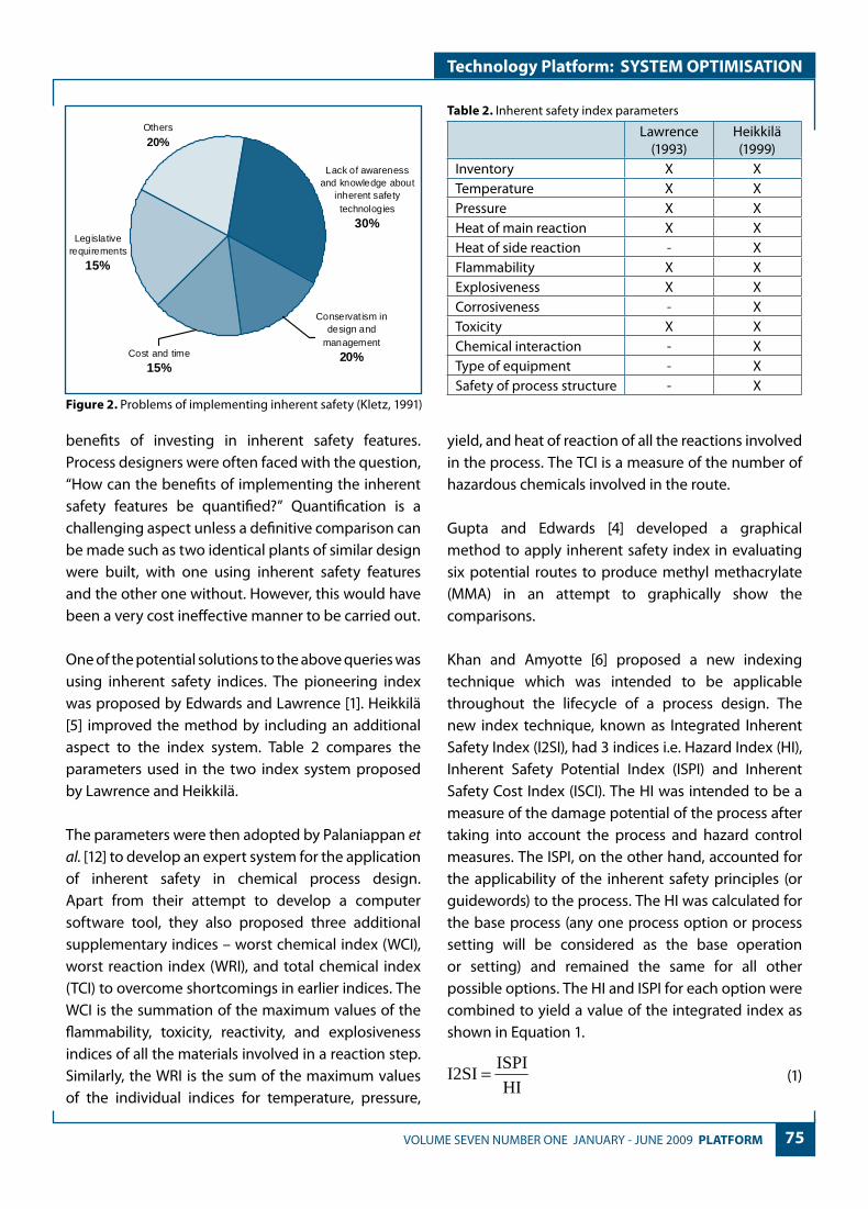
75 VOLUME SEVEN NUMBER ONE JANUARY - JUNE 2009 PLATFORM
Technology Platform: SYSTEM OPTIMISATION
benefits of investing in inherent safety features. Process designers were often faced with the question, “How can the benefits of implementing the inherent safety features be quantified?” Quantification is a challenging aspect unless a definitive comparison can be made such as two identical plants of similar design were built, with one using inherent safety features and the other one without. However, this would have been a very cost ineffective manner to be carried out.
One of the potential solutions to the above queries was using inherent safety indices. The pioneering index was proposed by Edwards and Lawrence [1]. Heikkilä [5] improved the method by including an additional aspect to the index system. Table 2 compares the parameters used in the two index system proposed by Lawrence and Heikkilä.
The parameters were then adopted by Palaniappan et al. [12] to develop an expert system for the application of inherent safety in chemical process design. Apart from their attempt to develop a computer software tool, they also proposed three additional supplementary indices – worst chemical index (WCI), worst reaction index (WRI), and total chemical index (TCI) to overcome shortcomings in earlier indices. The WCI is the summation of the maximum values of the flammability, toxicity, reactivity, and explosiveness indices of all the materials involved in a reaction step. Similarly, the WRI is the sum of the maximum values of the individual indices for temperature, pressure,
yield, and heat of reaction of all the reactions involved in the process. The TCI is a measure of the number of hazardous chemicals involved in the route.
Gupta and Edwards [4] developed a graphical method to apply inherent safety index in evaluating six potential routes to produce methyl methacrylate (MMA) in an attempt to graphically show the comparisons.
Khan and Amyotte [6] proposed a new indexing technique which was intended to be applicable throughout the lifecycle of a process design. The new index technique, known as Integrated Inherent Safety Index (I2SI), had 3 indices i.e. Hazard Index (HI), Inherent Safety Potential Index (ISPI) and Inherent Safety Cost Index (ISCI). The HI was intended to be a measure of the damage potential of the process after taking into account the process and hazard control measures. The ISPI, on the other hand, accounted for the applicability of the inherent safety principles (or guidewords) to the process. The HI was calculated for the base process (any one process option or process setting will be considered as the base operation or setting) and remained the same for all other possible options. The HI and ISPI for each option were combined to yield a value of the integrated index as shown in Equation 1.
HI
ISPII2SI = (1)
Conservatism in design and
management
20%Cost and time
15%
Legislative requirements
15%
Others
20%
Lack of awareness and knowledge about
inherent safety technologies
30%
Figure 2. Problems of implementing inherent safety (Kletz, 1991)
Table 2. Inherent safety index parameters
Lawrence (1993)
Heikkilä (1999)
Inventory X XTemperature X XPressure X XHeat of main reaction X XHeat of side reaction - XFlammability X XExplosiveness X XCorrosiveness - XToxicity X XChemical interaction - XType of equipment - XSafety of process structure - X
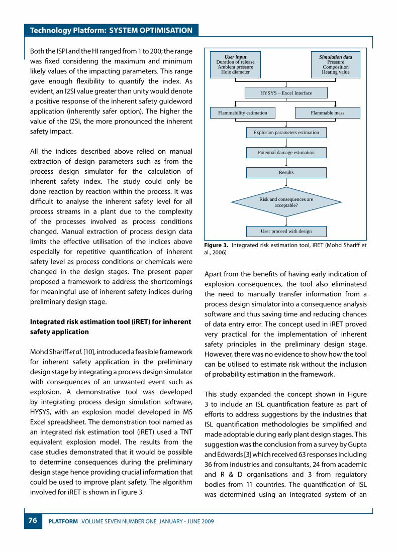
76 PLATFORM VOLUME SEVEN NUMBER ONE JANUARY - JUNE 2009
Technology Platform: SYSTEM OPTIMISATION
Both the ISPI and the HI ranged from 1 to 200; the range was fixed considering the maximum and minimum likely values of the impacting parameters. This range gave enough flexibility to quantify the index. As evident, an I2SI value greater than unity would denote a positive response of the inherent safety guideword application (inherently safer option). The higher the value of the I2SI, the more pronounced the inherent safety impact.
All the indices described above relied on manual extraction of design parameters such as from the process design simulator for the calculation of inherent safety index. The study could only be done reaction by reaction within the process. It was difficult to analyse the inherent safety level for all process streams in a plant due to the complexity of the processes involved as process conditions changed. Manual extraction of process design data limits the effective utilisation of the indices above especially for repetitive quantification of inherent safety level as process conditions or chemicals were changed in the design stages. The present paper proposed a framework to address the shortcomings for meaningful use of inherent safety indices during preliminary design stage.
Integrated risk estimation tool (iRET) for inherent safety application
Mohd Shariff et al. [10], introduced a feasible framework for inherent safety application in the preliminary design stage by integrating a process design simulator with consequences of an unwanted event such as explosion. A demonstrative tool was developed by integrating process design simulation software, HYSYS, with an explosion model developed in MS Excel spreadsheet. The demonstration tool named as an integrated risk estimation tool (iRET) used a TNT equivalent explosion model. The results from the case studies demonstrated that it would be possible to determine consequences during the preliminary design stage hence providing crucial information that could be used to improve plant safety. The algorithm involved for iRET is shown in Figure 3.
Apart from the benefits of having early indication of explosion consequences, the tool also eliminatesd the need to manually transfer information from a process design simulator into a consequence analysis software and thus saving time and reducing chances of data entry error. The concept used in iRET proved very practical for the implementation of inherent safety principles in the preliminary design stage. However, there was no evidence to show how the tool can be utilised to estimate risk without the inclusion of probability estimation in the framework.
This study expanded the concept shown in Figure 3 to include an ISL quantification feature as part of efforts to address suggestions by the industries that ISL quantification methodologies be simplified and made adoptable during early plant design stages. This suggestion was the conclusion from a survey by Gupta and Edwards [3] which received 63 responses including 36 from industries and consultants, 24 from academic and R & D organisations and 3 from regulatory bodies from 11 countries. The quantification of ISL was determined using an integrated system of an
Figure 3. Integrated risk estimation tool, iRET (Mohd Shariff et al., 2006)
User inputDuration of releaseAmbient pressure
Hole diameter
Simulation dataPressure
CompositionHeating value
HYSYS – Excel Interface
Explosion parameters estimation
Potential damage estimation
Results
Yes
User proceed with design
Flammable massFlammability estimation
Risk and consequences areacceptable?

77 VOLUME SEVEN NUMBER ONE JANUARY - JUNE 2009 PLATFORM
Technology Platform: SYSTEM OPTIMISATION
inherent safety index, consequences estimation and probability estimation with process design simulator.
INHERENT SAFETY LEVEL (ISL) qUANTIFICATION USING INHERENT SAFETY INDEX MODULE (ISIM)
The approach for the quantification of ISL followed the same concept as proposed by Mohd Shariff et al. [10]. A new framework was proposed to allow process information from a process design simulator, in this case HYSYS, to be extracted and analysed for the determination of inherent safety level, consequences and probability of unwanted incidences, as shown in Figure 4. The availability of such information at an early stage of design will help process designers to obtain ISL. The process designers can use the ISL as a tool to revise and produce safer designs by the application of the inherent safety concept in a more efficient and cost effective manner.
This paper discussed only the Inherent Safety Index Module (ISIM) as given in Figure 4 to demonstrate its feasibility to measure inherent safety levels during the
preliminary process design stage. Research is currently on-going to develop the entire framework and results will be published separately.
Data such as pressure, temperature, flow rate and composition were extracted from a process design simulator (in this case, HYSYS) using macros in Microsoft Excel to calculate inherent safety indices. Heikkilä’s classifications approach [5] was adopted as this method is very basic, easy to be implemented and does not require extensive use of proprietary monographs. Pressure, temperature and flow rate was directly evaluated for their respective inherent safety indices, ranging from 0 to 5 (worst). The composition of each stream was used to calculate the flammability limits of the mixture and translated to explosiveness. Based on the obtained indices, streams with unfavourable ISL were identified and improvements was carried out by process designers by applying one or more of the inherent safety principles as outlined in Table 1.
Figure 4. Framework to determine ISL at preliminary design stage
HYSYS Process Simulator
Inherent Safety IndexModule (ISIM)
This module evaluates the safety level. Will prompt the component of the index that
may be lowered.
Integrated ConsequenceEstimation Tool (ICET)
This module estimates consequences of an undesired
event. Can also evaluate multiple designs.
Integrated Probability Estimation Module (IPEM)
This module calculates the probability of the undesired event happening based on
established database.
Risk Factor CalculationRisk = consequences x probability
Acceptable?
Risk Comparison Criteria
Modify Design
NO
Further improve?
YESNO
Proceed With Design
YES
HYSYS Process Simulator
Inherent Safety IndexModule (ISIM)
This module evaluates the safety level. Will prompt the component of the index that
may be lowered.
Inherent Safety IndexModule (ISIM)
This module evaluates the safety level. Will prompt the component of the index that
may be lowered.
Integrated ConsequenceEstimation Tool (ICET)
This module estimates consequences of an undesired
event. Can also evaluate multiple designs.
Integrated ConsequenceEstimation Tool (ICET)
This module estimates consequences of an undesired
event. Can also evaluate multiple designs.
Integrated Probability Estimation Module (IPEM)
This module calculates the probability of the undesired event happening based on
established database.
Integrated Probability Estimation Module (IPEM)
This module calculates the probability of the undesired event happening based on
established database.
Risk Factor CalculationRisk = consequences x probability
Acceptable?
Risk Comparison Criteria
Modify Design
Further improve?
Proceed With Design

78 PLATFORM VOLUME SEVEN NUMBER ONE JANUARY - JUNE 2009
Technology Platform: SYSTEM OPTIMISATION
In the complete tool being developed currently, consequences and probability of unwanted incidents could also be assessed. By integration with a process simulator, it was expected that the impact of changes in process conditions to inherent safety levels and consequences can be effectively determined during the preliminary process design stage.
CASE STUDY
An acrylic acid production process was used as a case study to demonstrate the capability of ISIM for inherent safety application in the preliminary process design stage. The simulation model of an acrylic acid plant which was used in this case study was originally produced for academic purposes by Soo [14] using the HYSYS process design simulator. In this case study, ISIM was integrated with HYSYS to demonstrate its capability to determine stream that is more inherently unsafe. Design changes were than made to the identified stream following the principle of inherent safety for the improvement of safety level. For instance, a stream scoring a level 4 index was deemed to be more inherently unsafe compared to a stream scoring level 2. Since safety does not have an absolute level, the application of the As Low As Reasonable Practicable (ALARP) principle was necessary to reduce the index in conjunction with process requirements. For instance, if a process can only work at a particular temperature or pressure, which may score high index, other means of increasing safety level, should be explored rather than directly reducing pressure and/or temperature. This means not all scoring high index streams could be reduced to a lower index. Modification of the process conditions reached the limit once the desired process design objectives such as product quality were compromised.
The simulation process of the acrylic acid production plant had a total of 33 streams all together. The main feature of this acrylic acid production process was the twin parallel reactors (R101A and R101B) as shown in Figure 5 above that was capable of converting propene and air mixture into acrolein. Acrolein was further oxidised in another reactor to produce acrylic acid and other by-products. The mixture was further
refined in distillation towers to produce 99.99% pure acrylic acid.
In this case study, only the indices for temperature, pressure and explosiveness were considered in order to show the application of ISIM. Other parameters such as toxicity, corrosiveness, etc. were also important but not considered in this case study. The process information data for all 33 streams in the acrylic acid plant were easily transferred to ISIM due to the advantage of having integrated the system with HYSYS. The results of the indices were shown in Figure 6 to Figure 8 in order to illustrate the concept proposed in the framework. From these figures, it was observed that pressure parameters were all scoring index of 0, which meant that the system was operating at the low pressure regime and pressure was not an inherent safety concern for this process. Figure 7 and Figure 8 show that there were streams classified as level 3 and 4. At this point in time, there was no definitive manner to determine which level was safe or otherwise. It was concluded that a higher index was more inherently unsafe compared to a lower one. For the purpose of illustration, this case study was used to demonstrate how these streams could be modified to achieve a lower index.
Figure 5. Parallel reactors in original design of acrylic acid production plant (Soo, 2004)
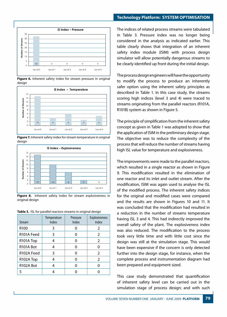
79 VOLUME SEVEN NUMBER ONE JANUARY - JUNE 2009 PLATFORM
Technology Platform: SYSTEM OPTIMISATION
The indices of related process streams were tabulated in Table 3. Pressure index was no longer being considered in the analysis as indicated earlier. This table clearly shows that integration of an inherent safety index module (ISIM) with process design simulator will allow potentially dangerous streams to be clearly identified up front during the initial design.
The process design engineers will have the opportunity to modify the process to produce an inherently safer option using the inherent safety principles as described in Table 1. In this case study, the streams scoring high indices (level 3 and 4) were traced to streams originating from the parallel reactors (R101A, R101B) system as shown in Figure 5.
The principle of simplification from the inherent safety concept as given in Table 1 was adopted to show that the application of ISIM in the preliminary design stage. The objective was to reduce the complexity of the process that will reduce the number of streams having high ISL value for temperature and explosiveness.
The improvements were made to the parallel reactors, which resulted in a single reactor as shown in Figure 9. This modification resulted in the elimination of one reactor and its inlet and outlet stream. After the modification, ISIM was again used to analyse the ISL of the modified process. The inherent safety indices for the original and modified cases were compared and the results are shown in Figures 10 and 11. It was concluded that the modification had resulted in a reduction in the number of streams temperature having ISL 3 and 4. This had indirectly improved the overall safety of the plant. The explosiveness index was also reduced. The modification to the process took very little time and with little cost since the design was still at the simulation stage. This would have been expensive if the concern is only detected further into the design stage, for instance, when the complete process and instrumentation diagram had been prepared and equipment sized.
This case study demonstrated that quantification of inherent safety level can be carried out in the simulation stage of process design; and with such
IS Index – Pressure
33 0 0 0 00
5
10
15
20
25
30
35
Lev el 0 Lev el 1 Lev el 2 Lev el 3 Lev el 4
Num
ber o
f Stre
ams
Num
ber o
f Stre
ams
IS Index – Temperature
0
2
4
6
8
10
12
14
16
Lev el 0 Lev el 1 Lev el 2 Lev el 3 Lev el 4
15 4 6 3 5
IS Index – Explosiveness
15 10 6 2 00
2
4
6
8
10
12
14
16
Lev el 0 Lev el 1 Lev el 2 Lev el 3 Lev el 4
Num
ber o
f Stre
ams
Figure 6. Inherent safety index for stream pressure in original design
Figure 7. Inherent safety index for stream temperature in original design
Figure 8. Inherent safety index for stream explosiveness in original design
Table 3. ISL for parallel reactors streams in original design
StreamTemperature
IndexPressure
IndexExplosiveness
Index
R100 3 0 2R101A Feed 3 0 2R101A Top 4 0 2R101A Bot 4 0 0R102A Feed 3 0 2R102A Top 4 0 2R102A Bot 4 0 05 4 0 0

80 PLATFORM VOLUME SEVEN NUMBER ONE JANUARY - JUNE 2009
Technology Platform: SYSTEM OPTIMISATION
information, an inherently safer design option can be proposed. In this particular case, the process was simplified by combining both reactors as one. From a mechanical and instrumentation stand point, lesser main equipment and lesser auxiliary equipment may improve overall reliability of the plant. It is important to stress that the final selection decision was made after considering other factors such as the economics of a larger reactor and operational flexibility of having only one reactor. The demerit of this design option was obvious in that the a larger inventory had to be handled by the single reactor.
It is very important to note that the application of different inherent safety principles to the same problem may arrive at different solutions in improving the safety level. It is better to consider all the relevant inherent safety principles according to the hierarchy proposed by Kletz [8] and careful consideration should be given to select the best solution in improving safety levels. As an example for
the case study of the reactor, it was not always that combining two reactors together would provide the best solution to improve safety levels. In the majority of times, multiple units rather than one big reactor will provide a better solution. Therefore, careful consideration and attention must be given in the application of inherent safety principles to ensure the best solution for the safest condition. Experience and knowledge on the design aspects are very important for effective application of the principles of inherent safety especially to review the agreement of different alternatives as highlighted by Moore [11].
A more detailed study is being carried-out to address the issues raised in this study. An enhanced safety index-determination technique is also being carried out which could be more suitably used with the proposed framework. A study using a heuristic approach is also on the way to provide easy application of inherent safety principles in the process design.
CONCLUSION
It was shown that an inherently safer process can be designed since the inherent safety level (ISL) of the original process can be determined at the preliminary design stage using a proposed Inherent Safety Index Module (ISIM) of a framework given in Figure 4. A more rigorous result could be determined once the entire system described in the framework given in Figure 4 is completed.
Figure 9. A modified processes with a single reactor
Inherent Safety Index – Temperature
0
2
4
6
8
10
12
14
16
Level 0 Level 1 Level 2 Level 3 Level 4
Nu
mbe
r of
Str
eam
s
ORIGINAL
MODIFIED
Inherent Safety Index – Explosiveness
0
2
4
6
8
10
12
14
16
Level 0 Level 1 Level 2 Level 3 Level 4
Nu
mbe
r of
Str
eam
s
ORIGINAL
MODIFIED
Figure 10. Inherent safety index for stream temperature in original and modified design
Figure 11. Inherent safety index for stream explosiveness in original and modified design
81 VOLUME SEVEN NUMBER ONE JANUARY - JUNE 2009 PLATFORM
Technology Platform: SYSTEM OPTIMISATION
ACKNOWLEDGEMENTThis paper is written in memory of our mentor; the late Professor Dr V. R. Radhakhrishnan who had contributed much thought and provided advice to the research group.
REFERENCES
[1] Edwards, D.W. and Lawrence, D., (1993). Assessing the inherent safety of chemical process routes: is there a relationship between plant costs and inherent safety? Trans IChemE, Part B, Process Safety and Environmental Protection, 71B, 252 – 258.
[2] Greenberg, H.H. and Cramer, J.J, (1991). Risk Assessment and Risk Management for the Chemical Process Industry, Van Nostrand Reinhold, New York.
[3] Gupta, J.P and Edwards, D.W. (2002). Inherently safer design – present and future, Trans. IChemE, Process Safety Environ. Protection B 80, 115.
[4] Gupta, J.P and Edwards, D.W. (2003), A simple graphical method for measuring inherent safety, Journal of Hazardous Materials, 104, 15–30.
[5] Heikkila, A.M. (1999). Inherent Safety in Process Plant Design, An Index-Based Approach, PhD Thesis, Helsinki University of Technology, Finland.
[6] Khan, F.I. and Amyotte, P.R. (2002). Inherent safety in offshore oil and gas activities: a review of the present status and future directions, Journal of Loss Prevention in the Process Industries, 15, 279-289.
[7] Khan, F.I. and Amyotte, P.R. (2004), Integrated inherent safety index (I2SI): A tool for inherent safety evaluation. Process Safety Progress, 23(2), 136-148.
[8] Kletz, T.A. (1991), Plant Design for Safety – A User Friendly Approach, 2nd edition; Taylor and Francis.
[9] Mansfield, D.P, Kletz T.A. and Al-Hassan, T. (1996), Optimizing safety by inherent offshore platform design, Proceeding of 1st International Conference on Health, Safety and Environment, The Hague, The Netherlands.
[10] Mohd Shariff, A., Rusli, R., Chan, T.L., Radhakrishnan, V. R., and Buang, A. (2006). Inherent safety tool for explosion consequences study, Journal of Loss Prevention in the Process Industries, 19, 409-418.
[11] Moore A.D. (1999). http://process-safety.tamu.edu/Research/Inherent%20Safety/Isappr.htm, (Accessed on 12 February 2006)
[12] Palaniappan, C., Srinivasan, R. and Tan, R. (2002). Expert system for the design of inherently safer processes. 2. Flowsheet development stage, Industrial & Engineering Chemistry Research, 41, 6711-6722.
[13] Rushton, A.G., Edwards, D.W. and Lawrence, D. (1994). Inherent safety and computer aided process design, Trans.IChemE, Part B 72 , 83 – 87.
[14] Soo, E.W. (2004). Acrylic Acid Production Plant, B.Eng. Final Year Plant Design Project, Universiti Teknologi PETRONAS, Malaysia.
[15] Taylor, J.R. (1994), Risk Analysis for process plant, pipelines and transport, E&FN Spon, UK.
[16] Zwetsloot, G.I.J.M., and Askounes Ashford, N. (1999). Encouraging inherently safer production in european firms: A report from the field, (Journal of Hazardous Materials), In A. Amendola and D. Wilkinson (Eds.) Special Issue on Risk Assessment and Environmental Decision Making, 123-144.
Azmi Mohd Shariff received his MSc in Process Integration from UMIST, United Kingdom in 1992. He furthered his studies at University of Leeds, United Kingdom and received his PhD in Chemical Engineering in 1995. He joined Universiti Kebangsaan Malaysia in 1989 as a tutor upon his return from Leeds and was appointed as lecturer in 1996.
He joined Universiti Teknologi PETRONAS (UTP) in 1997 and was appointed as the Head of Industrial Internship in 1998. He was later appointed as the Head of Chemical Engineering Programme 1999–2003. He is currently an Associate Professor in the Department of Chemical Engineering and a Leader of the Process Safety Research Group.
He teaches Process Safety and Loss Prevention at undergraduate level and Chemical Process Safety at graduate level. He started research work in the area of Process Safety in 2002. He has successfully supervised and is currently supervising a few PhD, MSc and final year undergraduate students in the area of Quantitative Risk Assessment (QRA), Inherent Safety and Behaviour Based Safety. He has presented and published more than 15 articles relating to process safety in conferences and journals. He currently leads an E-Science research project under Ministry of Science and Technology entitled ‘Development of Inherent Safety Software for Process Plant Design’. He has also experience in conducting QRA for a few local companies in Malaysia. Recently, he was successful in conducting a short-course on ‘Applied QRA in Process Industry’ to OPU and Non-OPU staff.

82 PLATFORM VOLUME SEVEN NUMBER ONE JANUARY - JUNE 2009
Technology Platform: SYSTEM OPTIMISATION
INTRODUCTION AND LITERATURE REVIEW
This research investigated the application of a formal mathematical optimisation approach of nonlinear programming (NLP) to the retrofitting of the water-utilisation and water-treatment operations of a real-world operational petroleum refinery. The
formulation is largely based on the mixed-integer nonlinear programming (MINLP) model proposed by Karuppiah and Grossmann [1] for the design of an integrated water network systems. An application of a mathematical optimisation approach to such problems was by Takama, Kuriyama, Shiroko, and Umeda [2], which addressed the optimal water
A COMPUTATIONAL PROCEDURE FOR SYSTEMATIC ANALYSIS OF WATER REUSE, REGENERATION AND RECYCLE IN
RETROFIT DESIGN OF REFINERY WATER NETWORK SYSTEMS
Khor Cheng Seong*Universiti Teknologi PETRONAS, 31750 Tronoh, Perak Darul Ridzuan, Malaysia
ABSTRACT
Water is a key element in the operation of petroleum refineries and petrochemical plants. Scarcities in freshwater supply and increasingly stringent rules on wastewater discharges have emerged as issues of major concerns to plant operators, along with an increased awareness in the need to support sustainable development initiatives and minimisation of water footprint. In line with these developments, a local refinery has included water reuse as part of its technology agenda, with the aim of minimising freshwater consumption and wastewater generation, through the approaches of water reuse, regeneration (i.e., treatment), and recycle (W3R). In particular, this paper is a report on a systematic procedure for carrying out a conceptual feasibility study to develop effective W3R strategies for water using processes and water treatment operations at the said refinery. The main thrust of the paper is to discuss the formulation and solution of a mathematical model with optimisation procedure in order to determine the optimal retrofit of the refinery water network systems. The integrated model explicitly considers the incorporation of water minimisation approaches and strategies by first postulating a superstructure that embeds all feasible flowsheet alternatives for the implementation of potential W3R opportunities using a modified version of the state-task network (STN) representation. Subsequently, a nonlinear programming (NLP) model was formulated based on the superstructure to determine the continuous variables of total stream flowrates and compositions. The key input to the model was the comprehensive water balance and wastewater characterisation data that was developed and conducted earlier. Computational studies were performed using the GAMS modeling language platform to obtain a feasible and optimal retrofit structure of the water network. The outcome from this modeling study was the development of W3R options inclusive of pretreatment requirement for reuse, which shall be further evaluated technoeconomically and subsequently implemented, where operationally-feasible.
Keywords: water reuse; water regeneration; water recycle; nonlinear programming (NLP); optimisation
This paper was presented at the International R&D Forum 2009, Kuala Lumpur, 25-27 May 2009

83 VOLUME SEVEN NUMBER ONE JANUARY - JUNE 2009 PLATFORM
Technology Platform: SYSTEM OPTIMISATION
allocation in a refinery. Other recent work that was considered for the use of optimisation include that of Alva-Argáez, Kokossis, and Smith [3] (MINLP), Hernández-Suárez, Castellanos-Fernández, and Zamora [4] (MINLP), Huang, Chang, Ling, and Chang [5] (NLP), and Galan and Grossmann [6] (MINLP).
MOTIVATION
Two reasons were the driving forces for undertaking this project. First, high demand of water in the future may result in an operating plant becoming vulnerable to water supply interruptions. Second, the work will support sustainable development, as exemplified by its goal of minimising freshwater consumption and wastewater generation in the water-using operations and water treatment units of a processing plant.
PROBLEM STATEMENT AND RESEARCH OBJECTIVES
The objective of this work was to formulate and solve a mathematical model that determines the optimal water flow network structure of a refinery which would satisfy the following three criteria: (1) minimum freshwater import; (2) minimum wastewater generation; and (3) contaminant concentrations within allowable limits. This will be achieved through the incorporation of water minimisation approaches and strategies which is reuse, regeneration, and recycle (W3R).
OPTIMISATION MODEL FORMULATION
Material Balances
The material balances on water flowrates and concentrations, or simply known as water balances, were constructed based on the total flows and contaminant compositions (concentrations) for each unit in the system, and they were categorised as follows:
Material Balances on Convergent-Flow-Path Units
in
out, , MUi k
i S
F F k S m∈
= ∀ ∈ ∀ ∈∑ (1)
in
, , out, , , MUi j i k j ki S
F C F C j k S m∈
= ∀ ∀ ∈ ∀ ∈∑ (2)
in
, , out, MU, ,j i j k
i S
f f m k S j J∈
= ∀ ∈ ∀ ∈ ∀ ∈∑ (3)
Material Balances on Divergent-Flow-Path Units
out
in, , SUi kk S
F F i S s∈
= ∀ ∈ ∀ ∈∑ (4)
out
in, , SUi kk S
F F i S s∈
= ∀ ∈ ∀ ∈∑ (5)
, , in out, , , , SUj i j kC C i S k S j s= ∀ ∈ ∀ ∈ ∀ ∀ ∈ (6)
Material Balances on Treatment Units
in out
, TUi ki S k S
F F t∈ ∈
= ∀ ∈∑ ∑ (7)
( )out in
, , ,1 , , TUj i j t j ki t k t
C R C j t∈ ∈
= − ∀ ∀ ∈∑ ∑ (8)
Material Balances on General Combined Convergent-and-Divergent-Flow-Path Units
in out
, GUi ki S k S
F F g∈ ∈
= ∀ ∈∑ ∑ (9)
in out
, , , , GUi j i k j ki S k S
FC F C j g∈ ∈
= ∀ ∀ ∈∑ ∑ (10)
Maximum Limit of Contaminant Concentrations for Recycle Streams
, freshwater, , , recyclei j jC C j J i′ ′≤ ∀ ∈ ∀ ∈ (11)maximum allowable concentrations of contaminant
Bounds on Variables
L Uin,i i iF F F i S≤ ≤ ∀ ∈ (12)
L Uout,k k kF F F k S≤ ≤ ∀ ∈ (13)
L U, , , in,j i j i j iC C C i S≤ ≤ ∀ ∈ (14)
L U, , , out,j k j k j kC C C k S≤ ≤ ∀ ∈ (15)
Non-negativity Constraints
, , in out, , , ,i k j i j kF F C C i S k S∀ ∈ ∀ ∈ (16)

84 PLATFORM VOLUME SEVEN NUMBER ONE JANUARY - JUNE 2009
Technology Platform: SYSTEM OPTIMISATION
Objective Function
In correspondence with the overall aim of the work undertaken, the criterion for the optimal solution was taken to be the minimisation of freshwater import and wastewater generation, which formed the objective function:
out
freshwater ,TU
min k tk S t
F F∈ ∈
+ ∑ ∑ (17)
IDENTIFICATION OF OPTIONS FOR POTENTIAL WATER REUSE, REGENERATION, AND RECYCLE (W3R)
The W3R alternatives options were formulated and postulated based on extensive discussions and deliberations with the plant engineers. Five alternatives were considered, as delineated in the following.
Base Case Alternative
The Base Case option was typically the most straightforward and easiest retrofitting option from a design point-of-view.
MT–CPI–C
OSW3 DAFuOSW1
Coke–RO(OS5)
PSR-1_Process_Area(OS8)
Sulfur_Run-o�(OS7)
Lift_Station-4(OS13)
OSW–SB
DAFs
S16
S9
MT –CPI–B
CPI–A
CPI–B
MT –CPI –A
OwiOWk
Owj
EFFLUENTTREATMENTSYSTEM (ETS)
CFuCarbonFilter
S10
Sand Filter
CLAs
ETS
SFs
Guard Basin (GBu)
S10–1S10–2
GBs
Discharge
GBrecycle
S17
RO3permeate
UF 3
UF3permeate
RO 3
RO3 reject1
To PSR-3
CFs
RO3 reject 2
SAMB
Potable (POT ) Toilets, kitchen, lab, eyewash (TKLE )
FIREWATER
PSR 1_SW
HPU 2
IonExchange
(IX)
SW 4
OW3C( Demin Regen )
CITY
Firewater FW
Potable Water POT
S1(splitter)
CITYWATER
CT 1
CT 2
SW 3
SW 1
CT3
S13
DT 1 WHB –BD 1
WHB –BD 2
OWg
S8
SW 2
Freshwater HPU 1Demin
Tank
DT 2
DEM
BOILER 1
SW 4–BDBL
Lost
To Demin
PSR 2_SW
Users
OSW4
OSW5
S11
BW1
BD1
OWa
Evap1
S3
S2
PSR -1CT
OW3A
BD2
BW2OW 20
Evap2
S5
S4
OW 18CogenCT
BD3
Evap 3
S7OWf
S6
BW 3
OWdMG 3
OWe–RG2
OW3B BDBLs 2BOILER
CITY 3
BDBLu(Sump
Pit)
BD1–BDBL 1
BW1–BDBL 2
BD2–BDBL 3L = 2
BW 2–BDBL 4
BD3 –BDBL 5
BW3–BDBL6
BDBLs 1
RG3–BDBL7
Existing structure
Proposed structure
Figure 1. Base Case alternative
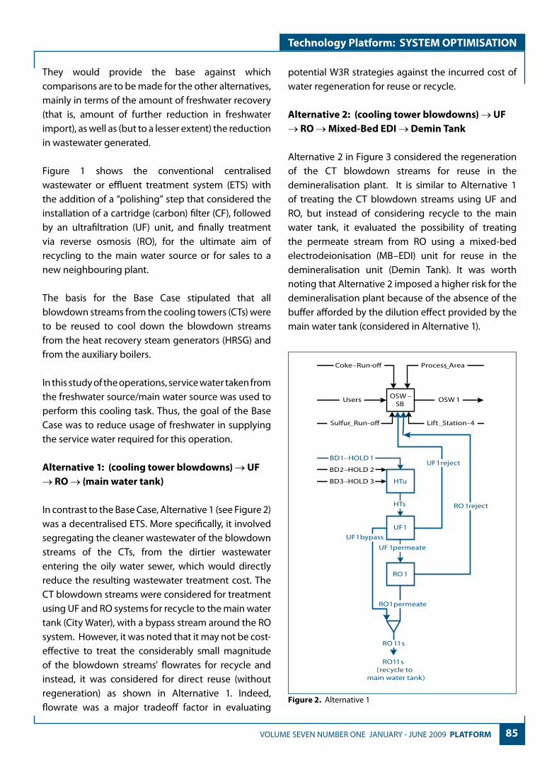
85 VOLUME SEVEN NUMBER ONE JANUARY - JUNE 2009 PLATFORM
Technology Platform: SYSTEM OPTIMISATION
They would provide the base against which comparisons are to be made for the other alternatives, mainly in terms of the amount of freshwater recovery (that is, amount of further reduction in freshwater import), as well as (but to a lesser extent) the reduction in wastewater generated.
Figure 1 shows the conventional centralised wastewater or effluent treatment system (ETS) with the addition of a “polishing” step that considered the installation of a cartridge (carbon) filter (CF), followed by an ultrafiltration (UF) unit, and finally treatment via reverse osmosis (RO), for the ultimate aim of recycling to the main water source or for sales to a new neighbouring plant.
The basis for the Base Case stipulated that all blowdown streams from the cooling towers (CTs) were to be reused to cool down the blowdown streams from the heat recovery steam generators (HRSG) and from the auxiliary boilers.
In this study of the operations, service water taken from the freshwater source/main water source was used to perform this cooling task. Thus, the goal of the Base Case was to reduce usage of freshwater in supplying the service water required for this operation.
Alternative 1: (cooling tower blowdowns) → UF → RO → (main water tank)
In contrast to the Base Case, Alternative 1 (see Figure 2) was a decentralised ETS. More specifically, it involved segregating the cleaner wastewater of the blowdown streams of the CTs, from the dirtier wastewater entering the oily water sewer, which would directly reduce the resulting wastewater treatment cost. The CT blowdown streams were considered for treatment using UF and RO systems for recycle to the main water tank (City Water), with a bypass stream around the RO system. However, it was noted that it may not be cost-effective to treat the considerably small magnitude of the blowdown streams' flowrates for recycle and instead, it was considered for direct reuse (without regeneration) as shown in Alternative 1. Indeed, flowrate was a major tradeoff factor in evaluating
potential W3R strategies against the incurred cost of water regeneration for reuse or recycle.
Alternative 2: (cooling tower blowdowns) → UF → RO → Mixed-Bed EDI → Demin Tank
Alternative 2 in Figure 3 considered the regeneration of the CT blowdown streams for reuse in the demineralisation plant. It is similar to Alternative 1 of treating the CT blowdown streams using UF and RO, but instead of considering recycle to the main water tank, it evaluated the possibility of treating the permeate stream from RO using a mixed-bed electrodeionisation (MB–EDI) unit for reuse in the demineralisation unit (Demin Tank). It was worth noting that Alternative 2 imposed a higher risk for the demineralisation plant because of the absence of the buffer afforded by the dilution effect provided by the main water tank (considered in Alternative 1).
Figure 2. Alternative 1
Users OSW 1
Coke–Run-o� Process_Area
Sulfur_Run-o� Lift_Station-4
OSW –SB
HTu
UF 1permeate
HTs
BD2–HOLD 2
BD3–HOLD 3
UF1
RO 1
RO 1reject
BD1– HOLD 1UF1reject
RO1permeate
UF1bypass
RO 11s
RO11s(recycle to
main water tank)

86 PLATFORM VOLUME SEVEN NUMBER ONE JANUARY - JUNE 2009
Technology Platform: SYSTEM OPTIMISATION
Alternative 3: Combinations of Alternatives 1 and 2
Alternative 3 (see Figure 4) was a combination of Alternatives 1 and 2. It served to evaluate the optimal split of flows for incorporating both the options of recycle to main water tank and reuse in the demineralisation tank.
Alternative 4
Alternative 4 seen in Figure 5 considered the possibility of recycling to the main water source; first, by segregating the cleaner wastewater generated from the utilities (i.e., the blowdown and backwash streams from the CTs), which were first fed into the oily water sewer ballast tank and by mixing them with the
DT 2
DEM
RO 12s
EDI–1
EDI–3
MB–EDIs
RejRO–EDI
BOILER 1
RO –EDI
MB–EDIu
DeminTank
HTu
UF 1permeate
HTs
BD2–HOLD2
BD3–HOLD3
UF 1
RO 1 RO 1reject
BD1– HOLD1
UF 1reject
RO 1permeate
UF 1bypass
RO11s
ToCogen CT
Figure 3. Alternative 2
Figure 5. Alternative 4
Figure 4. Alternative 3
DT 2
DEM
RO12s
EDI–1
EDI–3
MB–EDIs
RejRO–EDI
BOILER 1
RO –EDI
MB –EDIu
DeminTank
HTu
UF1permeate
HTs
BD2–HOLD 2
BD3–HOLD 3
UF 1
RO1 RO 1reject
BD1– HOLD1
UF 1reject
RO 1permeate
UF1bypass
RO11s
S12
RO 13s(recycled to
main water tank)
ToCogen CT
OS3
M4u(mixer)
CFuCarbonFilter
S10
Sand Filter
CLAs
M4sETS
SF
Guard Basin (GBu)
S10 –1S10–2
GBs
Discharge
GBrecycle
S17
WATERREGENERATION
S18
MMF OS4
UF 2 permeate
UF 2
RO2reject1
RO 2
RO2reject2
RO3reject2
RO 2 permeate
Recycle toCITYWATER
HTs 2
MT –CPI–
COSW 3 DAFu
OSW1100
BD3–HOLD 3 HTu
BD2–HOLD 2
BD1–HOLD 1
Coke–RO(OS5)
PSR -1_Process_Area(OS8)
Sulfur_Run-o�(OS7)
Lift _Station-4(OS13)
OSW –SB
RO2reject3

87 VOLUME SEVEN NUMBER ONE JANUARY - JUNE 2009 PLATFORM
Technology Platform: SYSTEM OPTIMISATION
oily surface water in a storm basin. This was followed by regeneration using a sequence of the existing treatment units comprising mud trap, corrugated plate interceptor, and dissolved air flotation. Finally, Alternative 4 assessed the proposed subsequent regeneration technologies which consisted of a multimedia filter (MMF), UF, and RO, before recycling to the main water tank. In comparison with the other options, this alternative considered the feasibility of MMF for removal of total dissolved solids in contributing towards water recovery for reuse and/or to meet environmental regulations for discharge, without regeneration via the ETS.
COMPUTATIONAL RESULTS AND DISCUSSION
All alternatives were conceptually feasible in achieving reduction in freshwater import and wastewater generation, provided that pre-treatment for oil and grease removal was implemented in all cases, where a suitable pre-treatment technology needed to be identified. A potential pre-treatment technology was the use of a membrane bioreactor (MBR). Other conventional oil and grease removal technologies included corrugated plate interceptor (CPI) and dissolved air flotation (DAF).
However, the alternatives were still subject to further rigorous techno-commercialisation evaluation before the detailed design could be carried out. In addition, the numerical results pointed towards the potential of considering W3R strategies for the process water portion where the sources included sour water, process condensates, storm water (from process units), oil drains, sampling effluents from process units and the tankages (tanks), tankage water draining, desalter water, and mud wash.
CONCLUSION
It appeared that the main challenge for the successful implementation of water reuse, regeneration, and recycle initiatives in a refinery concerns the removal of oil and grease according to its minimum allowable concentration limit or tolerance. In summary, the formal mathematical optimisation approach was
capable of evaluating the feasibility and optimality of W3R alternatives. However, it would suffice to caution that the use of mathematical programming should be to the extent of mainly providing insights on the available alternatives. The computed values of flowrates and concentrations were reliable in providing a sense of magnitude of the expected operating values.
SETS AND INDICESI' set of materials or products iJ set of contaminants jSin set of inlet streams iSout set of outlet streams kMU set of convergent-flow-path units (mixers) mSU set of divergent-flow-path units (splitters)s sTU set of treatment unit tGU set of general combined convergent-and-divergent-flow-
path units g
PARAMETERS
Rj,t removal ratio of contaminant j in treatment unit tL
iF lower bound on flowrate in stream iU
iF upper bound on flowrate in stream iL,j iC lower bound on contaminant concentration j in stream i
U,j iC upper bound on contaminant concentration j in stream i
CONTINUOUS VARIABLES
Fi flowrate of inlet stream i
Fk flowrate of outlet stream k
fj,i flowrate of contaminant j in stream i
Cj,i concentration of contaminant j in stream i
ACKNOWLEDGEMENTThe author gratefully acknowledges the contribution from the many parties who have been instrumental in carrying out this work to completion: (1) PETRONAS Penapisan (Melaka) Sdn Bhd (PP(M)SB) for providing the financial support; (2) the industrial inputs provided by the plant engineers especially Norliza Abang Zamhari (PP(M)SB) and Siti Norzamiah Nadzmi (PETRONAS Group Technology Solutions (GTS)), as well as that of Sarina Tukiman (GTS), M Saiful Tajudin, Suhaimi Zaid, and Rahmat C Razib (all from PP(M)SB); (3) Pei Chie Leong, the undergraduate research assistant especially for executing most of the computational tasks involved in this work; and (4) Universiti Teknologi PETRONAS for the full support of this work. Parts of this work was presented at the PETRONAS 3rd International R&D Forum 2009 and the 4th PETRONAS Water Technology Conference 2009.

88 PLATFORM VOLUME SEVEN NUMBER ONE JANUARY - JUNE 2009
Technology Platform: SYSTEM OPTIMISATION
REFERENCES
[1] R. Karuppiah, I. E. Grossmann, Global optimization for the synthesis of integrated water systems in chemical processes, Comp. Chem. Eng. 30 (2006) 650–673.
[2] Takama, N., Y. Kuriyama, K. Shiroko, and T. Umeda. Optimal water allocation in a petrochemical refinery. Computers & Chemical Engineering 4 (1980): 251–258.
[3] A. Alva-Argáez, A. C. Kokossis, R. Smith, The design of water-using systems in petroleum refining using a water-pinch decomposition, Chemical Engineering Journal 128 (2007): 33–46.
[4] R. Hernández-Suárez, J. Castellanos-Fernández, J. M. Zamora, Superstructure decomposition and parametric optimization approach for the synthesis of distributed wastewater treatment networks, Industrial & Engineering Chemistry Research 43 (2004): 2175–2191.
[5] C.-H. Huang, C.-T. Chang, H.-C. Ling, C.-C. Chang, A mathematical programming model for water usage and treatment network design, Industrial & Engineering Chemistry Research 38 (1999): 2666–2679.
[6] B. Galan, I. E. Grossmann, Optimal design of distributed wastewater treatment networks, Industrial & Engineering Chemistry Research 37 (1998): 4036–4048.
Khor Cheng Seong is a lecturer and researcher in the Chemical Engineering Department of Universiti Teknologi PETRONAS. He obtained his Master of Applied Science (MASc) degree in chemical engineering with specialization in process systems engineering from the University of Waterloo, Ontario, Canada. He also holds the Certificate in University Teaching
diploma from the same institution. His area of research interests lies at the interface of chemical engineering, systems engineering, and operations research. His research work addresses problems related to the design, planning, and scheduling of process energy systems and water systems through the development of optimisation-based mathematical models, tools, and strategies. In addition, he is also interested in the incorporation of the systems approach in chemical engineering education, learning theory in higher education, and the national systems of innovation on a whole. He has recently published a book entitled “Optimization Strategies for Petroleum Refinery Planning under Uncertainty: A Hybrid of Stochastic Programming Approaches with Economic and Operational Risk Management”.
Leong Pei Chie graduated with a Bachelor of Engineering (Honours) degree in Chemical Engineering in the year 2009. She is currently a production engineer in the capacity of a field planner at the Peninsular Malaysia Operations (PMO) of the Operations Division of PETRONAS Carigali Sdn. Bhd.
Siti Norzamiah Nadzmi is a water and wastewater technical professional (TP) with Process Engineering of Group Technology Solutions (GTS) of PETRONAS Research and Technology (R&T). She has extensive consulting experience with various water and wastewater treatment issues and operations within PETRONAS. She is a member of the PETRONAS Water Steering Committee.
Norliza Zamhari is the manager of the Utilities, Treating, Energy, and Environment Section of the Technology Department of PETRONAS Penapisan (Melaka) Sdn. Bhd. She is one of the most respected figures in the water and wastewater technology community in PETRONAS and is a prominent member of the PETRONAS Water Steering Committee.

89 VOLUME SEVEN NUMBER ONE JANUARY - JUNE 2009 PLATFORM
Technology Platform: SYSTEM OPTIMISATION
INTRODUCTION
Natural gas (NG) has recently emerged as an important source of clean energy. Production of NG involves a series of cooling and heating processes of feed gas (FG) in a refrigerated gas plant (RGP). FG is expanded to improve recovery of natural gas liquids (NGLs). To meet the pipeline specification, an end-product called sales gas (SG) is recompressed before leaving the RGP. SG consists of mainly methane and some ethane, while NGLs comprise ethane and heavier components.
Improving the operational efficiency of an RGP may significantly increase its profit margin. A proportional-integral (PI) control scheme was currently used for maintaining process variables at their respective set point values. However, large amounts of energy was required for this purpose. A more advanced controller in the form of the model predictive control (MPC) has been known to be able to reduce operating costs.
A lot of research work has been published in the case of employing MPC in industrial case studies. For example, a commercial package called DMCPlus was used to design and implement an MPC scheme in a propane-propylene splitter comprising 182 trays [1]. In a refinery case, the MPC scheme was designed for a crude distillation unit (CDU) based on a HYSYS dynamic model [2].
In this paper, a 2x2 constrained MPC scheme was developed for an RGP. The dynamic model of an RGP developed by Yusoff et al. [3] was used to perform virtual plant testing and control in HYSYS. The underlying process models were obtained using the prediction error method. The MPC action was calculated in MATLAB. Linking between HYSYS and MATLAB was made possible through the component object module (COM) technology. The performance of the MPC was compared to the PI control in several cases of set point tracking.
A COMPARISON BETWEEN MPC AND PI CONTROLLERS ACTING ON A REFRIGERATED GAS PLANT
Nooryusmiza Yusoff* and M. RamasamyUniversiti Teknologi PETRONAS, 31750 Tronoh, Perak Darul Ridzuan, Malaysia
ABSTRACT
A refrigerated gas plant (RGP) produces sales gas (SG), which is the preferred fuel of power plants. Sustaining SG production at an optimum cost is crucial to an RGP posed with operational challenges. These challenges may be alleviated by adopting a model predictive control (MPC) scheme. In this research, a 2x2 constrained MPC scheme was developed. RGP process dynamics were approximated by first-order-plus-time-delay models. Performance of the MPC scheme was compared with a decentralised proportional integral (PI) control scheme in set point tracking. Although the PI controller seemed to perform better than the MPC controller, its performance was achieved at a higher operating cost and hence reduced RGP profit.
Keywords: refrigerated gas plant, model predictive control, regulatory control
This paper was presented at the International Conference on Control, Instrumentation and Mechatronic Engineering (CIM09), Malacca, 2 - 3 June 2009

90 PLATFORM VOLUME SEVEN NUMBER ONE JANUARY - JUNE 2009
Technology Platform: SYSTEM OPTIMISATION
MPC FORMULATION
The MPC objective was to minimise a quadratic function written in the following compact form [4]:
}||||||{||||||)(1
0
22
1
2 ∑∑−
=++
=+ ++=
M
jjk
ujk
P
j
yjk
MSRQ ∆ueeuJ (1)
subject to the following linear constraints:
max,min, jjkj yyy ≤≤ + , Pj ,...,1=∀ (2a)
max,min, jjkj ∆u∆u∆u ≤≤ + , 1,...,0 −=∀ Mj (2b)
max,min, jjkj uuu ≤≤ + , 1,...,0 −=∀ Mj (2c)
and subject to the observability of an augmented state estimator xk+1|k proposed by Muske and Badgwell [5]:
kkkkk BuAxx +=+ ||1 (3)
where
)( 1|1|| −− −+= kkmkfkkkk yyKxx
(4a)
1|1| −− = kkkk Cxy (4b)
The convention used for weighted 2-norm terms in the objective function was Qeee Q
T=2|||| . The notation
1| −kkx referred to the state estimate at time step k given the information available up to time step k−1. State estimate xk|k provided a feedback mechanism to the system since it included a term comparing current measured output m
ky to current predicted output 1| −kky
. Gain Kf was obtained by solving Kalman filter design.
The solution to the optimisation problem (Equation 1) was a sequence of M input moves:
},...,,{ 11 −++= MkkkM uuuu (5)
In practice, however, only the first input move uk would be implemented at each control action in order to update state estimate xk+1|k. The remaining calculated moves },...,{ 11 −++ Mkk uu were discarded. In subsequent control actions, this process was repeated at each time step.
RESULTS AND DISCUSSION
MPC Setup
The first step in setting up an MPC controller was to obtain process models. Here, a traditional approach of open-loop step testing was implemented. Responses of outputs y:y=[y1 y2] due to step changes
0 100 200 300 400 500 600 700 800 900 1000 1100-34
-33
-32
y 1 (o C
)
0 100 200 300 400 500 600 700 800 900 1000 11000
5
10
y 2 (o C
)
0 100 200 300 400 500 600 700 800 900 1000 1100
74
76
78
u 1 (%
)
0 100 200 300 400 500 600 700 800 900 1000 110062
64
66
u 2 (%
)
Time (min)
Figure 1. Open-loop responses for step changes in input u1.

91 VOLUME SEVEN NUMBER ONE JANUARY - JUNE 2009 PLATFORM
Technology Platform: SYSTEM OPTIMISATION
of inputs u:u=[u1 u2] were plotted in Figures 1 and 2. In each test, an input was stepped by 3% of the controller output after 100 min of simulation time, returned to the nominal condition after 500 min and maintained there for another 500 min. In essence, a total of 1 100 min was taken for each step test. The long duration ensures that steady-state output values were reached in each step test. Outputs were measured simultaneously during each input move, in order to capture their dynamic responses due to that particular input.
From observations of Figures 1 and 2, all open-loop responses resembled the behavior of first-order-plus-time-delay (FOPTD) model below:
1p,
p,d,
+=
−
s
eKg
ij
sij
ij
ij
τ
τ
(6)
The notation gij referred to the transfer function relating output yi to input uj. Kp,ij and τp,ij were process gain and time constant, respectively. Time delay was given by τd,ij. The process gains, time constants and time delays obtained for this system are given in Table 1.
Once models were identified, the MPC controller was designed by specifying constraints and several
0 100 200 300 400 500 600 700 800 900 1000 1100-34.5
-34
-33.5
y 1 (o C
)
0 100 200 300 400 500 600 700 800 900 1000 1100
-20
0
20
y 2 (o C
)
0 100 200 300 400 500 600 700 800 900 1000 110076
77
78
u 1 (%
)
0 100 200 300 400 500 600 700 800 900 1000 110060
65
u 2 (%
)
Time (min)
Figure 2. Open-loop responses for step changes in input u2.
Table 1. FOPTD model parameters.
Transfer Function
Model Parameters
Kp (ºC/%) τp (min) τd (min)
g11 –0.26 24.5 0
g12 0.26 38.9 5.5
g21 –1.70 18.8 16.4
g22 2.69 26.6 1.7
Table 2. MPC design and tuning parameters.
Parameters ValuesControl interval 1 minControl horizon, M 2Prediction horizon, P 120Weighting matrices:• Output, Q diag [1 1]• Input rate, R diag [0.15 0.1]• Input, S diag [0 0]Constraints:• Output, y [–5 5; -5 5]• Input rate, ∆u [–5 5; –5 5]• Input, u [–25 25; –25 25]

92 PLATFORM VOLUME SEVEN NUMBER ONE JANUARY - JUNE 2009
Technology Platform: SYSTEM OPTIMISATION
parameters as shown in Table 2. Parameters were selected after several closed-loop simulation studies were performed under different process conditions. The MPC controller was built on top of two decentralised PI controllers, TC101 and TC102, which were previously employed to regulate the respective E-102 (chiller) and E-104 (reboiler) duties. The PI controller was tuned based on the Auto Tune Variation (ATV) technique of Astrom and Hagglund [6]. Values of the PI controller tuning parameters are listed in Table 3.
Set Point Tracking
A good controller should be able to change an output from its nominal value to another state smoothly. This process is termed set point tracking. In this work, the integral of squared error (ISE) was used to compare the performance of the MPC and PI controllers. Nominal input and output values are given in Table 4. Input
cost was calculated by assuming linear relationship between the controller output duty (%) and the actual duty (kW) for each input (Table 5). Total simulation time for all cases of set point tracking was 250 min.
0 10 20 30 40 50 60 70 80 90 100-35
-34.5
-34
-33.5
y 1 (o C
)
0 10 20 30 40 50 60 70 80 90 1003
4
5
6
y 2 (o C
)
0 10 20 30 40 50 60 70 80 90 10075
80
85
90
u 1 (%
)
0 10 20 30 40 50 60 70 80 90 10060
65
70
u 2 (%
)
Time (min)
MPC
PISP
MPC
PISP
MPC
PINom.
MPC
PINom.
Figure 3. Closed-loop responses for a change in y1 (Case 1).
Table 3. PI controller parameters.
Controller Parameters
Controller Kc (oC/%) τ I (min)
TC101 0.31 0.32
TC102 0.91 9.70
Table 4. Nominal input and output values.
Index Input (%) Output (oC)
1 77.0 -33.8
2 64.3 4.8
Table 5. Ranges of actual input duty values.
Input Minimum (kW) Maximum (kW)
u1 0 4200
u2 0 4500
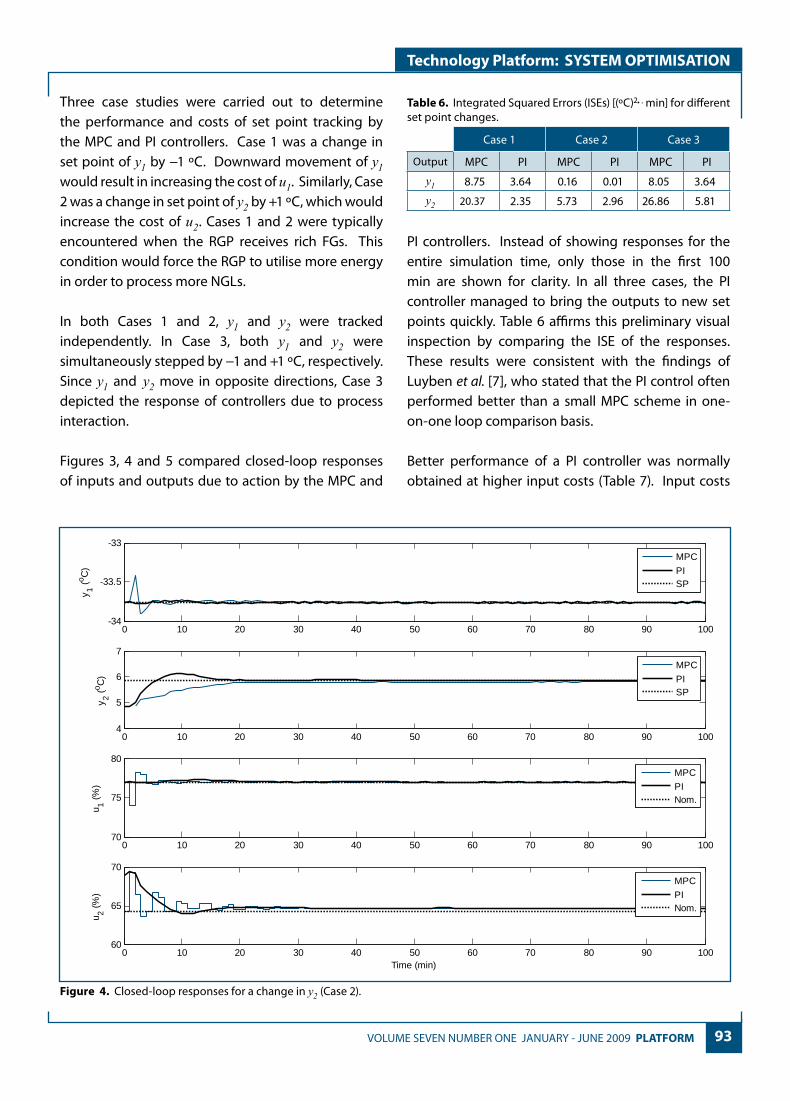
93 VOLUME SEVEN NUMBER ONE JANUARY - JUNE 2009 PLATFORM
Technology Platform: SYSTEM OPTIMISATION
Three case studies were carried out to determine the performance and costs of set point tracking by the MPC and PI controllers. Case 1 was a change in set point of y1 by −1 ºC. Downward movement of y1 would result in increasing the cost of u1. Similarly, Case 2 was a change in set point of y2 by +1 ºC, which would increase the cost of u2. Cases 1 and 2 were typically encountered when the RGP receives rich FGs. This condition would force the RGP to utilise more energy in order to process more NGLs.
In both Cases 1 and 2, y1 and y2 were tracked independently. In Case 3, both y1 and y2 were simultaneously stepped by −1 and +1 ºC, respectively. Since y1 and y2 move in opposite directions, Case 3 depicted the response of controllers due to process interaction.
Figures 3, 4 and 5 compared closed-loop responses of inputs and outputs due to action by the MPC and
PI controllers. Instead of showing responses for the entire simulation time, only those in the first 100 min are shown for clarity. In all three cases, the PI controller managed to bring the outputs to new set points quickly. Table 6 affirms this preliminary visual inspection by comparing the ISE of the responses. These results were consistent with the findings of Luyben et al. [7], who stated that the PI control often performed better than a small MPC scheme in one-on-one loop comparison basis.
Better performance of a PI controller was normally obtained at higher input costs (Table 7). Input costs
0 10 20 30 40 50 60 70 80 90 100-34
-33.5
-33
y 1 (o C
)
0 10 20 30 40 50 60 70 80 90 1004
5
6
7
y 2 (o C
)
0 10 20 30 40 50 60 70 80 90 10070
75
80
u 1 (%
)
0 10 20 30 40 50 60 70 80 90 10060
65
70
u 2 (%
)
Time (min)
MPC
PISP
MPC
PISP
MPC
PINom.
MPC
PINom.
Figure 4. Closed-loop responses for a change in y2 (Case 2).
Table 6. Integrated Squared Errors (ISEs) [(ºC)2⋅. min] for different set point changes.
Case 1 Case 2 Case 3
Output MPC PI MPC PI MPC PI
y1 8.75 3.64 0.16 0.01 8.05 3.64
y2 20.37 2.35 5.73 2.96 26.86 5.81

94 PLATFORM VOLUME SEVEN NUMBER ONE JANUARY - JUNE 2009
Technology Platform: SYSTEM OPTIMISATION
were calculated as a deviation of controller moves from their corresponding initial steady-state (nominal) values with respect to simulation time of 250 min. These costs included refrigeration and reboiler duties as tabulated by Yusoff et al. [8]. Controller moves above nominal values increased operational costs while those below nominal values decreased it. Hence, negative values of cost may be incurred such as the one in Case 2 for the u1 move under the MPCscheme. This phenomenon indicated cost savings from refrigeration consumption. In Cases 1, 2 and 3, moves of the PI controller respectively cost 9.9%, 14.2% and 9.0% higher than that of the MPC controller. This result was not surprising due to the decentralised nature of PI controllers, in which one input moves independently from the other. Conversely, the MPC controller provided coordinated moves for u1 and u2.This is carried out so that, for example, if y1 were toremain at the previous set point, y2 would reach thenew set point in an optimal manner.
CONCLUSION
A cost reduction effort for RGP that implements MPC scheme is illustrated. Performance of MPC controller is compared with that of decentralized PI controllers in term of set-point tracking. MPC controller results in a lower operating cost as compared with PI controllers. It is also observed that PI controllers yield smaller ISEs on output variables. However, this is only achieved at higher input costs, which reduce RGP profit margin.
0 10 20 30 40 50 60 70 80 90 100-35
-34.5
-34
-33.5
y 1 (o C
)
0 10 20 30 40 50 60 70 80 90 1004
5
6
7
y 2 (o C
)
0 10 20 30 40 50 60 70 80 90 10075
80
85
90
u 1 (%
)
0 10 20 30 40 50 60 70 80 90 10060
65
70
u 2 (%
)
Time (min)
MPC
PISP
MPC
PISP
MPC
PINom.
MPC
PINom.
Figure 5. Closed-loop responses for simultaneous changes in y1 and y2 (Case 3).
Table 7. Costs (RM’000) of input changes for different set point changes.
Case 1 Case 2 Case 3
Input MPC PI MPC PI MPC PI
u1 153.5 169.0 -0.03 0.27 154.8 169.3
u2 22.3 24.2 4.96 5.36 27.6 29.6
Total 175.8 193.2 4.93 5.63 182.4 198.9
95 VOLUME SEVEN NUMBER ONE JANUARY - JUNE 2009 PLATFORM
Technology Platform: SYSTEM OPTIMISATION
ACKNOWLEDGMENTThe authors are grateful for financial support from Universiti Teknologi PETRONAS.
REFERENCES
[1] Alsop N. and Ferrer J.M. (2006). “Step-test free APC implementation using dynamic simulation”. AIChE Spring National Meeting, Orlando, Florida.
[2] Pannocchia G., Gallinelli L., Brambilla A., Marchetti G. and Trivella F. (2006). “Rigorous simulation and model predictive control of a crude distillation unit.” ADCHEM. Gramado, Brazil.
[3] Yusoff N., M. Ramasamy, Yusup S. (2008). “A simulation study on dynamics and control of a refrigerated gas plant.” FOCAPO. Boston, MA.
[4] Qin S.J. and Badgwell T.A. (2003). A survey of industrial model predictive control technology.” Control Engineering Practice, 11, 733-764.
[5] Muske K.R. and Badgwell T.A. (2002). “Disturbance modeling for offset-free linear model predictive control.” Journal of Process Control, 12, 617–632.
[6] Astrom K.J. and Hagglund T. (1984). Automatic tuning of simple regulators with specifications on phase and amplitude margins. Automatica, 20, 645.
[7] Luyben W.L., Tyreus B.D. and Luyben M.L. (1999). Plantwide process control. McGraw-Hill: New York.
[8] Yusoff N., M. Ramasamy, Yusup S. (2007). “Profit optimization of a refrigerated gas plant.” ENCON. Kuching, Sarawak, Malaysia.
Nooryusmiza Yusoff graduated from Northwestern University, USA with BSc Degree in Chemical Engineering and subsequently became a member of the American Chemical Engineering Honors Society “Omega Chi Epsilon”. He received the MSc Degree from the University of Calgary, Canada with a thesis on applying geostatistical analyses in predicting ozone
temporal trends. He is currently pursuing his PhD at the Universiti Teknologi PETRONAS (UTP) after serving as a lecturer in the Department of Chemical Engineering, UTP. His areas of research interest centre on process modeling and simulation, advanced process control as well as planning and scheduling.
Dr M. Ramasamy is presently an Associate Professor in the Department of Chemical Engineering at Universiti Teknologi PETRONAS (UTP). He graduated from Madras University in the year 1984. He obtained his masters degree with specialisation in Process Simulation, Optimisation and Control from the Indian Institute of Technology, Kharagpur in 1986.
In 1996, he received his PhD from the Indian Institute of Technology, Madras. His areas of research interests include modeling, optimisation and advanced process control. Dr Ramasamy has guided several undergraduate and postgraduate students and published/presented several technical papers in international refereed journals, international and national conferences. He has delivered a number of special lectures and also successfully organised seminars/symposiums at the national level. Presently, he is the project leader for the PRF funded project on “Optimization of Energy Recovery in Crude Preheat Train” and eScience funded project on soft sensor development.