Please do not quote.

ON THE SOCIAL DESIRABILITY OF

URBAN RAIL TRANSIT SYSTEMS

Clifford Winston Vikram Maheshri Brookings Institution U.C. Berkeley

December 2005

1

Introduction

The evolution of urban rail transit in the United States over the past twenty years

has been marked by three inescapable facts that signal an inefficient allocation of transit

resources. Rail’s share of urban travelers is declining; its deficits are rising sharply; and

yet investment to build new systems and extend old ones continues.

In 1980, two million Americans got to work by rail transit. Today, in spite of an

increase in urban jobs and transit coverage, fewer than one million U.S. workers use rail,

causing its share of work trips to drop from 5 percent to 1 percent.1 Although rail

transit’s farebox revenues have consistently failed to cover its operating and capital costs

since World War II, governmental aid to cover transit deficits has been increasingly

available. Since 1980, operating subsidies have climbed from $6 billion to more than $15

billion today (APTA Transit Fact Books, figures in 2001 dollars). Capital subsidies have

also increased as transit agencies struggle to maintain and provide new facilities, track,

and rolling stock.

These worrisome trends, however, have not curbed U.S. cities’ appetite for rail

transit service. During the 1990s, Cleveland, Washington, Santa Clara, Sacramento and

other cities expanded their systems, while Los Angeles, Denver, Dallas, and St. Louis

built new ones. Recently, Houston and Minneapolis opened new light rail lines while

small, sparsely populated cities such as Sioux City, Harrisburg, and Staunton, Virginia

suggested that they want federal funds to help build their systems. And although county

residents repeatedly nixed a referendum to build a $4 billion extension of Washington’s

Metro out to Dulles airport, planners nevertheless circumvented popular will and diverted

1 These figures are from the National Transit Database and the U.S. Census.

2

increased toll revenue from the Dulles toll road to finance a portion of the ultimate

extension.

Any private firm that was losing market share and reporting increasing losses

would be hard pressed to attract funds to expand. Almost certainly, it would try to

determine the most efficient way to contract. Of course, a transit agency does not seek to

maximize profits, but its public financing is justified only if it is raising social welfare,

where social welfare can be measured as the difference between net benefits to

consumers and the agency’s budget deficit, also taking into account externalities of rail

transit (for instance, the reduction in roadway congestion attributable to rail.)

Although the costs and benefits of public rail transit operations have been debated

in the policy community (see, for example, Litman (2004)), we are not aware of a recent

comprehensive empirical assessment of rail’s social desirability.2 The purpose of this

paper is to estimate the contribution of each U.S. urban rail operation to social welfare

based on the demand for and cost of its service. We find that with the single exception of

BART in the San Francisco Bay area, every U.S. transit system actually reduces social

welfare. Worse, we cannot identify an optimal pricing policy or physical restructuring of

the rail network that would enhance any system’s social desirability without effectively

eliminating its service.

Rail transit’s problem is its failure to attract sufficient patronage to reduce its high

average costs. This problem has been complicated enormously by new patterns of urban

2 Richmond (2001) provides an overview of U.S. rail transit systems including their ridership and financial performance. Winston and Shirley (1998) estimate the net benefits of urban rail systems as of 1990. Other researchers such as Savage (2004), Savage and Schupp(1997), Kain (1997), and Viton (1981) have assessed the welfare properties of and alternative polices to improve specific transit systems.

3

development. Rail operations, unfortunately, are best suited for yesterday’s concentrated

central city residential developments and employment opportunities; they are decidedly

not suited for today’s geographically dispersed residences and jobs. At best, urban rail

service may be socially desirable in a few large U.S. cities if its operations can be

adjusted to mirror successful privatization experiments conducted abroad. Ironically,

however, rail transit enjoys powerful political support from planners, civic boosters, and

policymakers, making it highly unlikely that rail’s social cost will abate.

An Empirical Framework for Estimating Rail Transit’s Social Benefits

Urban rail transit operators do not set prices to cover operating and capital costs.

In fact, under Federal Transit Administration Section 5307, transit fares (including bus,

rail, and paratransit) have to cover only some 17 percent of operating costs for most

agencies to qualify for federal funds. State and municipal funding thresholds vary, but

none requires even half of operating costs to be covered at the farebox. On average, the

nation’s rail transit systems cover only about 40 percent of operating costs, to say nothing

of their substantial capital costs (National Transit database). Like any good or service,

rail’s net benefits to users are simply given by consumer surplus, but to justify continued

operation, rail’s surplus must offset the difference between farebox revenues and costs.3

We develop rail transit demand and cost models to estimate users’ benefits and

agencies’ budget deficits. We also account for rail’s effect on the cost of roadway

congestion. A novel feature of the models is that they include variables that characterize

3 Rail transit also directly generates a small portion of its revenues from advertisements, parking lot fees, and other auxiliary services. We explicitly exclude these revenue streams and their associated production costs when we perform our analysis.

4

a transit system’s network configuration and stations, enabling us to explore whether rail

could enhance its social benefits by expanding or contracting its facilities in an efficient

manner.4

Demand. Our empirical analysis is conducted on a panel of U.S. urban rail transit

systems. We specify travelers’ demand (in passenger miles) for rail transportation, DitQ ,

on system i during year t as:

);,,( itititDit

Dit uXZpDQ = , (1)

where Ditp is the average fare, itZ contains exogenous network variables, itX contains

exogenous city characteristics, and itu is an error term.5

Depending on the system, transit fare is determined by a transit agency,

metropolitan planning organization, or city council. It is therefore reasonable to treat fare

as exogenous because it is primarily determined through a regulatory process rather than

market forces. In addition, the policy bodies that set fares have little incentive to adjust

them to changing market conditions because they are not subject to stringent financial

performance goals.

Rail demand is also influenced by the configuration of a transit system’s network.

Travelers are more likely to use rail if it provides more comprehensive coverage of a

4 An alternative (indirect) measure of rail transit’s benefits is rail’s impact on housing prices in the surrounding residential area near stations. Diaz (1999) summarizes studies of the effect that some systems have had on residential property values. Baum-Snow and Kahn (2000) provide a recent study. 5 We will interchange the term city with urbanized area and metropolitan (statistical) area (MSA). Urbanized areas and MSAs are determined by U.S. Census demographic criteria; nonetheless, they are often associated with a distinct city. Data on rail transit systems tend to pertain to a metropolitan statistical area.

5

given area, offers more conveniently located stations, offers more connectivity, and

accommodates travel in both north-south and east-west directions (i.e., its network is

nonlinear). The following components of a transit network enable us to derive four

metrics from graph theory to capture the effect of a rail system’s entire network on

demand:6

n number of stations served (nodes);

e number of station to station links (edges);

lp,q length of a particular link from station p to station q;

d length of the shortest route between the farthest two stations (diameter);

A total land area served by the system.

Based on these components, the relevant network variables are:

∑≠

=qp

qplA

D ,1 , indicating the density of the network. A network has greater

density if it provides more track length in its service area.

∑≠

=qp

qple ,1η , indicating the average length of all links in the network. Smaller

values of η indicate that stations tend to be closer together, which can be convenient for

travelers.

63 −=Γ

ne , a measure of connectivity that considers the relationship between the

actual number of links and the maximal number of links, given a set of stations. Greater

connectivity can improve access to different points on the network.

6 Hagget and Chorley (1969) provide a complete discussion of the measures.

6

∑≠

=qp

qpld ,1π , indicating the (non)-“linearity” of the network. The measure takes

on a minimum value of one, characterizing a perfectly linear network. Larger values

characterize less linearity and thus broader coverage of a given geographical area.

We also characterize rail’s service with the ratio of its peak service frequency to

base service frequency.7 Because rail and bus systems are often designed to complement

each other, we also control for bus transit’s peak-to-base ratio. Larger rail and bus

frequency peak-to-base ratios should increase demand.

Turning to the characteristics of a city that may influence rail demand, we control

for regional gasoline prices, the average number of days below 32 degrees Fahrenheit,

and the average commute time. Higher gasoline prices may induce commuters to switch

from driving, which would increase transit use, but they may also depress overall

economic activity, which would tend to decrease transit use. Thus, the a priori effect of

gasoline price is ambiguous. Cold temperatures tend to increase transit ridership because

they discourage commuters, in particular, from walking and biking. A high average

commute time in a city is likely to be caused by lengthy work-trip distances and factors

that contribute to road congestion. The former may reduce travelers’ accessibility to rail

and decrease the demand for transit, while the latter may increase the demand for rail

transit as travelers try to avoid congestion. Thus, the a priori effect of average commute 7 The peak service frequency is defined as the maximum average frequency of the 7-10am morning and 4-7pm evening rush hours. The base service frequency is defined as the average frequency of the 10am-4pm off-peak period. It is reasonable to treat the frequency ratio as exogenous because the timing and duration of the peak are fixed and not influenced by demand, while peak and off-peak schedules are largely determined by labor contracts. We also tried to capture service frequency by specifying a system’s vehicle miles (seat miles are not available), but the peak-to-base frequency ratio produced more plausible and reliable estimates.

7

time is also ambiguous.8 Finally, we include the metropolitan area population and

resident households’ median annual income. Demand for rail transit should be positively

related to an area’s population. Although transit is often regarded as an inferior good, the

average income of travelers who use rail is much higher than the average income of

travelers who use bus (Winston and Shirley (1998)), so rail transit may be a normal

good.9

Cost. Regulations constrain rail transit agencies from abandoning or adding track

and stations to optimize their operations; hence, it is inappropriate to assume that they are

in long-run equilibrium. We therefore specify a short-run total cost function where we

include the network variables discussed previously to control for the capital inputs of

track and stations that are fixed in the short-run. Formally, short run total costs, Cit, for

transit system i during year t are expressed as:

);,,,( itititititit YZwQCC ν= , (2)

8 It is possible that average commute times may be higher in cities that have a measurable share of rail transit users, which would suggest that average commute time may be endogenous. We consider this possibility in our estimations. 9 We explored some additional and alternative variables to capture service quality and city characteristics. Because heavy rail systems can operate at higher speeds than light rail systems, we included a dummy variable for systems with predominantly heavy rail service, but it was statistically insignificant. For climate effects, we also specified average snowfall and a light rail dummy variable interacted with snowfall or cold temperatures because light rail stations tend to be above ground. These variables were insignificant. We also specified average commute distance instead of average travel time to work, but it was poorly measured and had virtually no effect on demand. Finally, we specified a dummy variable for new systems—those that had operated for five years or less—to explore whether some travelers might be attracted to rail because of its novelty. However, the dummy was statistically insignificant.

8

where itQ is output in passenger miles, itw contains factor prices, itZ contains exogenous

network variables, itY contains other exogenous influences on cost, and itν is an error

term.10

Given that fares can be assumed to be exogenous, it is reasonable to treat output

as exogenous in the cost function.11 We include factor prices for labor and fuel. The

price of labor is given by the hourly wage for transit workers, including fringe benefits.

Because different rail transit systems use different combinations of fuel types (gas,

electricity, kerosene, ethanol, and so on), we computed a standardized price per kilowatt-

hour of energy using the appropriate physical constants (i.e., KWH equivalents) for each

one.12 We capture the effect of capital on short-run costs by including the network

variables that we used in the demand model. Holding output constant, we expect

networks with greater density, connectivity, or more closely situated stations to have

higher costs. The a priori effect of network linearity on costs is not clear; greater

linearity requires a system to use less rolling stock to serve its stations, while greater non-

linearity may enable a system to achieve higher load factors that would reduce costs.

10 Urban rail transit cost functions have been estimated previously by Pozdena and Merewitz (1978), Viton (1980), and Savage (1997). 11 Although absolute measures of peak and off-peak passenger miles were not available, we tried to specify peak and off-peak output by interacting passenger miles with peak-to-base ratios, but this did not enable us to obtain reliable estimates of distinct outputs. We also specified peak and off-peak vehicle miles (as noted, seat miles were not available), but these measures of capacity are apparently too crude to improve the model. We also tried to control for different “qualities” of output by including the heavy rail dummy noted in footnote 9 to capture potentially faster travel times provided by systems that offered predominantly heavy rail service, but the dummy was insignificant. 12 We interacted the heavy rail dummy with fuel price because heavy and light rail have different fuel intensities, but the interaction term was statistically insignificant.

9

Finally, the other exogenous variables we include in the cost function are transit system

age and the average number of days below 32 degrees Fahrenheit. Newer systems may

depreciate less rapidly than older systems but have higher operating costs.13 Colder

climates are likely to accelerate the depreciation of a transit system’s capital stock but

have an uncertain effect on operating costs.

Sample. We include the twenty-five U.S. urban rail transit systems that were in

operation between 1993 and 2000 generating 194 observations (a few systems began

operations midway through the decade).14 These systems are distinct from various

commuter rail systems in the nation that mainly link distant suburbs and nearby urban

areas to a city’s rail and bus transit system. The sample accounts for all urban travel by

light and heavy rail transit during the period. Data sources for the variables used in the

demand and cost models and summary statistics are presented in table 1. Short-run total

costs are defined as the sum of operating costs and depreciation and amortization of rail

transit capital. To construct the network variables, we obtained annual transit network

maps for each system and traced their expansion using detailed city maps. It is useful to

note that although our sample includes twenty-five systems, trips on New York City’s

system account for roughly two-thirds of the nation’s rail transit passenger miles.

13 In our sample discussed below, system age and the costs of depreciation are positively related. The age of a transit system is based on the year that a system began offering rail service to the public. 14 We began our panel in 1993 because some variables in the National Transit Database were defined differently before that year. We did not extend our sample beyond 2000 because we thought it would be difficult to obtain long-lived information about the welfare properties of transit systems in the tumultuous period that followed. Finally, we did not include the King County (Seattle) transit system and the Detroit Metropolitan transit system because they just began rail operations in 2000.

Table 1. Variables and Summary Statistics* Variable Mean Minimum Maximum Source Fare per passenger mile 0.197 0.101 0.393 National Transit Database Short Run Total Costs(millions)**

393 2.84 4370 National Transit Database

Passenger Miles (millions)** 528 2.63 8320 National Transit Database Total Track (miles)** 118.2 8.3 834.2 National Transit Database Total Stations** 60.4 9 469 Transit System Network

Maps Service Area (square miles)** 1132 48.6 6559 National Transit Database Links Between Stations** 57.74 8 482 Transit System Network

Maps Transit System Age (years) 30.79 0 103 Transit System Agencies Average Energy Cost per KWH

0.002 0.001 0.009 National Transit Database

Average Hourly Wage plus Benefits

32.14 9.89 50.25 National Transit Database

Metropolitan Area Population (millions) **

3.713 1.17 9.52 US Census Bureau

Median Annual Household Income

50,613 37,665 65,673 Texas A&M Real Estate Center

Average Regional Gasoline Price per Gallon

1.44 1.24 1.67 US Depart. of Energy, Annual Energy Review

Average Travel Time to Work (minutes) **

25.24 19.4 31.1 Dept. of Transportation, Journey to Work Survey

Average Number of Days Annually Below 32° F

63.2 0 156 National Meteorological Survey

Rail Peak-to-Base Ratio 2.21 0.23 8 National Transit Database Bus Peak-to-Base Ratio*** 1.85 1 3.4 National Transit Database Number of Observations 194 * Fares, costs, wages, and incomes are in 2000 dollars. ** Maximum value corresponds to the New York City Transit Agency.*** In the few cities where multiple bus systems served the rail transit agency’s service area, we selected the largest bus system.

10

Accordingly, the maximum values in the table for costs, output, and physical

characteristics of the system correspond to the NYC transit agency.

Estimation Results

We explored various functional forms for the demand model including linear, log-

linear, and flexible forms with interacted network variables. The best statistical fit, which

also captured the heterogeneity of the systems, was obtained with a simple linear

functional form that allowed the coefficients for fares and the network variables to vary

by system size. As noted, the New York City system is quite extensive and carries far

more passengers than any other system. This system along with the Washington, San

Francisco, Chicago, Philadelphia, Boston, Atlanta, and Northern New Jersey systems

comprise the so-called “Big 8” U.S. transit systems; we therefore identified distinct

effects for New York’s system and defined “large” systems to include the other seven

systems. We then divided the remaining seventeen systems into seven “medium”

systems and ten “small” systems.15

15 Large systems were defined as having more than 250 million passenger-miles annually. These systems included Washington, DC Metro, BART (SF Bay Area), Chicago Transit, MBTA (Boston), MARTA (Atlanta), SEPTA (Philadelphia) and PATH (Northern New Jersey). Medium systems were defined as having between 70 million and 250 million passenger-miles annually. These systems included GCRT (Cleveland), MTA (Baltimore), PATCO (Southern New Jersey), San Francisco Municipal Railway, San Diego Trolley Inc., Los Angeles Metro and Metro-Dade Transit (Miami). Small systems were defined as having between 2 million and 70 million passenger-miles annually. These systems included TriMet (Portland, OR), Santa Clara Co. Transit (San Jose), Staten Island Rapid Transit, Sacramento Regional Transit, Niagara Frontier Metro (Buffalo), Bi-State Development Agency (St. Louis), DART (Dallas), PA Alleghany Co. (Pittsburgh), RTD (Denver) and NJTransit (Newark).

11

Estimation results are presented in table 2. We controlled for fixed system, state,

and year effects, but only the year effects were statistically significant so they are

included in the final model. The high R2 is not attributable to any particular

socioeconomic characteristic(s) that may be believed to correlate strongly with passenger

demand. For example, when we omitted population from the specification, the R2 was

still quite high; a small decrease in R2 also occurred when we omitted income. Note that

a strong relationship between rail transit demand and population does not always exist

(e.g., Los Angeles has a large population, but small transit ridership, while the opposite is

true for Cleveland).

Turning to the coefficients, average fares have a negative and statistically

significant effect on demand. The demand elasticities, computed by sample enumeration,

are -1.3 for New York City, -0.97 for the large systems, -5.4 for medium systems, and

-3.2 for small systems. Previous studies of large urban transit systems based on data in

the 1970s and early 1980s tended to find that the demand for rail was inelastic (Winston

(1985) and Small (1992) provide surveys). However, given that these systems now offer

more extensive suburban service and that populations in a metropolitan area are more

geographically dispersed, rail faces more intense competition from auto, which would

cause the demand elasticity to increase. For instance, Voith (1991) estimates that the

elasticity of demand for the SEPTA commuter rail system, which includes but is not

limited to serving Philadelphia, is -1.6. In addition, real transit fares have risen

substantially in the past two decades, which would also cause the demand elasticity to

Table 2. Demand Coefficients, 1993-2000* Dependent variable is billions of passenger miles

Variable NYC Transit

Large Systems1

Medium Systems2

Small Systems3

Fare ($) -37.1 (12.0)

-1.48 (0.442)

-3.44 (1.02)

-0.495 (0.181)

Track density (D) 0.544 (0.114)

0.544 (0.114)

0.061 (0.113)

-0.184 (0.177)

Average distance between stations (η)

-0.112 (0.049)

-0.112 (0.049)

-0.137 (0.040)

-0.115 (0.045)

Network connectivity (Γ) 4.94 (1.58)

4.94 (1.58)

0.013 (0.086)

0.206 (0.139)

Network linearity (π) (Greater values indicate less linearity)

0.090 (0.023)

0.090 (0.023)

0.017 (0.015)

0.016 (0.013)

Constant 10.6 (3.43)

1.43 (1.75)

3.56 (1.47)

2.92 (1.39)

Common Parameters Rail peak-to-base ratio 0.053

(0.027)

Bus peak-to-base-ratio 0.180 (0.055)

Average number of days below 32 degrees

0.002 (0.001)

Metropolitan area population (millions)

0.023 (0.012)

Median household income in metro area ($thousands)

0.003 (0.003)

Average regional gasoline price ($)

-0.371 (0.278)

Average travel time to work (minutes)

-0.218 (0.091)

Average travel time to work squared

0.004 (0.002)

Year Dummies Included Number of Observations 194 R2 0.991 *Huber-White Robust Standard Errors provided in parentheses.

1 Large systems include Washington, DC Metro, BART (SF Bay Area), Chicago Transit, MBTA (Boston), MARTA (Atlanta), SEPTA (Philadelphia) and PATH (Northern New Jersey). 2 Medium systems include GCRT (Cleveland), MTA (Baltimore), PATCO (Southern New Jersey), San Francisco Municipal Railway, San Diego Trolley Inc., Los Angeles Metro and Metro-Dade Transit (Miami). 3 Small systems include TriMet (Portland, OR), Santa Clara Co. Transit (San Jose), Staten Island Rapid Transit, Sacramento Regional Transit, Niagara Frontier Metro (Buffalo), Bi-State Development Agency (St. Louis), DART (Dallas), PA Alleghany Co. (Pittsburgh), RTD (Denver) and NJTransit (Newark).

12

increase.16 It is therefore plausible that we now find that the demand elasticity for New

York City and the large systems clusters around unity, with the New York City system

having the most elastic demand among these systems because many travelers have the

option of using auto, taxi, bus, or even walking to get to their destinations.17

Medium and small rail systems have a tiny share of travelers in the cities they

serve (less than 1 percent), which undoubtedly contributes to their high elasticity of

demand (i.e., modest responses in ridership to fare changes are proportionally large for

smaller rail transit systems). In addition, these systems face considerable competition

from auto because they operate in cities where residential and commercial development is

predominantly influenced by and caters to automobile transportation. Despite their

dependence on the auto, cities with medium and small rail systems tend to experience

less congestion than cities with large rail systems.

The network variables for New York City and the large systems are statistically

significant and have their expected signs. (We find that the coefficients are not

statistically significantly different for these systems.) Greater track density, connectivity,

and (non) linearity increase demand for rail, while a greater average distance between

stations reduces demand. Greater average distances between stations also reduce demand

for rail in medium and small systems. But the other network variables tend to have

16 According to the American Public Transit Association, real average transit (bus and rail) fares have increased 37.3 percent from 1980 to 2000. Unfortunately, data for just rail fares are not available during this period. In any case, the increase in transit fares undoubtedly reflects an increase in rail fares. 17 According to Federal Highway Administration Means of Travel to Work survey in 2000, New York City leads the nation in the share of commuters who get to work by bus (6.8 percent), by walking or biking (5.9 percent), or by taking a taxi (0.8 percent).

13

statistically insignificant effects on demand, possibly because these systems are not well-

developed and compete only for a small and specialized segment of travelers.

We do not reject the hypothesis that each of the remaining influences has the

same effect on demand across rail transit systems. As expected, we find that an increase

in the peak-to-base frequency ratio for rail or bus increases rail demand and that cities

with larger populations and that experience more days below freezing have more rail

users.18 Rail demand is also positively related to a city’s median household income,

indicating that rail transit is a normal good, but the effect is not precisely estimated. We

find that the decline in real gas prices during our sample period caused rail demand to

increase. This finding is consistent with the notion that gas prices tend to affect transit

use by influencing the overall level of economic activity. In addition, because most

suburban-based rail trips are combined with an auto trip, lower gas prices could increase

rail demand by expanding its catchment area (Baum-Snow and Kahn (2005)). Finally,

we find that the demand for rail decreases as average commute time increases, but this

effect diminishes as commutes get longer and travelers are more willing to shift to rail to

avoid roadway congestion even if they have to drive to outlying stations.19

18 It is possible that the weather variable is actually capturing a “rust belt/sun belt” effect of traditional cities in the northeast versus the more auto-friendly cities of the west and south. However, its effect persisted when we included regional dummies in the specification. Those dummies tended to be insignificant. 19 If the mode share of rail transit were influencing average commute time, we would expect that commutes that take longer would be associated with more demand for rail. However, we find the opposite relationship between commute time and demand, suggesting that average commute time is likely to be exogenous because of rail’s small mode share. As a further check, we estimated a model that specified average auto commute time, which would be more likely than average commute time to be exogenous. We found that this variable had little effect on the coefficients, although t-statistics were somewhat lower than those using average commute time.

14

We initially explored estimating a cost function for rail transit using either a

translog or quadratic flexible functional form along with factor demand equations for fuel

and labor. However, we found that most of the interaction terms were poorly estimated

and that the predictions of transit costs were implausible because New York City’s

dominant system made it impossible to specify a meaningful average (mean) transit

system for the country. Hence, we settled on a simple, linear specification that fit the

data well and produced plausible predictions of transit costs.

The coefficient estimates are presented in table 3. Final estimations include state

and year fixed effects (system fixed effects were statistically insignificant, possibly

because the twenty-five systems in our sample are located in only thirteen distinct states

and most transit systems within a state are subject to the same state regulations). In

contrast to the demand model, we do not find that any of the determinants of short-run

total cost vary by system size. Consistent with the presence of large deficits, the

estimated marginal cost per passenger mile of 65 cents is considerably above the average

fare per passenger mile of 20 cents reported in table 1. The short-run scale elasticity,

based on enumerating the ratio of the estimated marginal cost coefficient to average costs

for each system in the sample, was 1.45 for New York City transit and 0.96 for the

remaining systems. These estimates indicate that none of the systems is operating at

minimum cost.20 Part of the problem is likely to be rail transit’s low average load

factor—less than 20 percent as of the mid-1990s (Winston and Shirley (1998)). Since

then, the Federal Transit Authority has stopped requiring transit systems to report load

factor data.

20 Our findings are broadly consistent with Viton (1980), who finds diseconomies for the New York City system and slight scale economies for some smaller systems.

Table 3. Cost Coefficients, 1993-2000* Dependent variable is total cost in millions of dollars Variable Coefficient Passenger-miles (millions)

0.648 (0.051)

Energy price per KWH ($)

7250 (5950)

Hourly wage plus benefits ($)

2.183 (1.773)

Track density (D)

124 (74.5)

Network connectivity (Γ)

103 (44.2)

Average distance between stations (η)

-20.4 (17.0)

Network linearity (π) (Greater values indicate less linearity)

-40.8 (16.0)

Average number of days below 32° F

-2.250 (1.497)

Transit system age

-9.047 (2.816)

Average number of days below 32° F * Transit system age

0.168 (0.043)

Constant

514 (300)

Year Dummies Included State Dummies Included Number of Observations 194 R2 0.961 *Huber-White Robust Standard Errors provided in parentheses.

15

Although some of the coefficients for the factor prices and network variables are

imprecisely estimated, all of these influences have their expected signs. Increases in fuel

prices and wages raise costs. Greater track density and connectivity raise the cost of a

system, while costs fall as distances between stations increase and as a network becomes

more nonlinear. Finally, we find that system age and weather are inversely related to

costs but that these variables have interactive effects that may increase costs. Newer

systems may have higher operating costs than older systems because they use more costly

technologically sophisticated equipment and their agencies have less experience in

troubleshooting these systems. On the other hand, older systems depreciate at faster rates

than newer systems. Weather therefore interacts with system age because colder climates

accelerate the deprecation of a system’s capital stock.21

Net Benefits of Urban Rail Transit Systems

The net benefits of an urban rail transit system are the difference between users’

consumer surplus and agency deficits that must be covered by publicly funded subsidies.

(We will account for externalities later.) Given the inverse of our estimated demand

function, p(q), and the estimated short-run cost function, C, evaluated at the equilibrium

output, q*, we can express a system’s net benefits, NB, as:

( ) ( ) ( )***

0

*

*

qCqpqpdqqpqNBq

−⋅+⎟⎟

⎠

⎞

⎜⎜

⎝

⎛⋅−= ∫ . (3)

21 The weather variable may also be capturing regional differences in costs. But its effect persisted when we included regional dummies to the specification. We could not obtain reliable estimates of both regional and state dummies; we obtained a better fit and greater statistical significance using the state dummies instead of the regional dummies.

16

A valid concern can be raised about the reliability of calculating net benefits in

this fashion because we are integrating our estimated demand curve from values of q=0

over the equilibrium output levels. But as shown in figure 1, the vast majority of our data

points lie in a small neighborhood around q=0, implying that our coefficients are most

reliable at small levels of traffic. In addition, it is highly unlikely that demand could be

infinite around q=0 because urban travelers do not place a large value on rail compared

with their next best alternative (Winston and Shirley (1998)). According to the 2001

National Household Travel Survey, the median annual incomes of rail users exceed

$50,000, which indicates it would misleading to suggest that a perceptible fraction may

be captive to rail because they cannot afford a car.22 As traffic levels significantly

expand, calculation errors have a much smaller effect on the estimated triangular region

of surplus because the area that is added falls with the square of q.

In table 4, we present estimates of the net benefits for each system in the year

2000.23 Although New York City’s transit system and some of the large systems do

22 Median annual incomes of rail transit users may be considerably higher than $50,000 because the highest income bracket reported in the National Household Travel Survey is “greater than $50,000.” 23 The estimates measure the absolute rather than the marginal benefits to travelers provided by rail. Thus, we are overestimating rail’s benefits because if rail transit were eliminated, some users would shift to other modes of transportation and their loss in consumer surplus would only be the difference between the consumer surplus from rail and the consumer surplus from the next best modal alternative. On the other hand, we are also underestimating rail’s benefits to some extent because some travelers who never use rail may nonetheless value it as an (unexercised) option. Given rail’s very small market share (indicating its lack of competitiveness with auto) and its low likelihood of being a viable alternative for the many travelers who do not live and work sufficiently close to rail stations, our measure is most certainly overestimating rail benefits more than it is underestimating them. Thus, rail’s actual benefits are likely to be smaller than estimated here.

Figure 1. Fares and Traffic on US Rail Transit Networks, 1993-2000*

0

0.1

0.2

0.3

0.4

0.5

0 2 4 6 8 10

Passenger Miles (billions)

Fare

per

pas

seng

er m

ile (2

000

dolla

rs)

* The eight outlying points correspond to the New York City Transit Agency, which serves roughly two thirds of total national rail transit traffic.

17

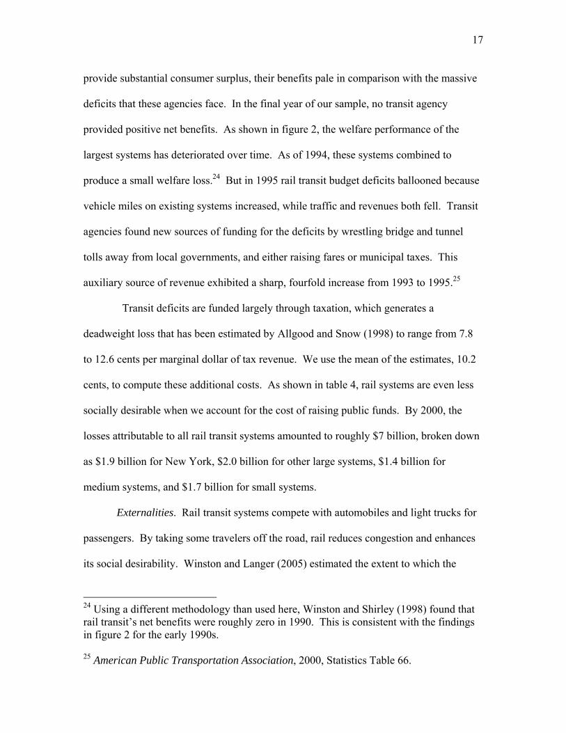
provide substantial consumer surplus, their benefits pale in comparison with the massive

deficits that these agencies face. In the final year of our sample, no transit agency

provided positive net benefits. As shown in figure 2, the welfare performance of the

largest systems has deteriorated over time. As of 1994, these systems combined to

produce a small welfare loss.24 But in 1995 rail transit budget deficits ballooned because

vehicle miles on existing systems increased, while traffic and revenues both fell. Transit

agencies found new sources of funding for the deficits by wrestling bridge and tunnel

tolls away from local governments, and either raising fares or municipal taxes. This

auxiliary source of revenue exhibited a sharp, fourfold increase from 1993 to 1995.25

Transit deficits are funded largely through taxation, which generates a

deadweight loss that has been estimated by Allgood and Snow (1998) to range from 7.8

to 12.6 cents per marginal dollar of tax revenue. We use the mean of the estimates, 10.2

cents, to compute these additional costs. As shown in table 4, rail systems are even less

socially desirable when we account for the cost of raising public funds. By 2000, the

losses attributable to all rail transit systems amounted to roughly $7 billion, broken down

as $1.9 billion for New York, $2.0 billion for other large systems, $1.4 billion for

medium systems, and $1.7 billion for small systems.

Externalities. Rail transit systems compete with automobiles and light trucks for

passengers. By taking some travelers off the road, rail reduces congestion and enhances

its social desirability. Winston and Langer (2005) estimated the extent to which the

24 Using a different methodology than used here, Winston and Shirley (1998) found that rail transit’s net benefits were roughly zero in 1990. This is consistent with the findings in figure 2 for the early 1990s. 25 American Public Transportation Association, 2000, Statistics Table 66.

Table 4. Social Net Benefits of Transit, 2000* (Figures in parentheses include an exhaustive public spending cost of 10.2%)

City (Agency)

Consumer Surplus

Transit Agency Deficit

Net Benefits Congestion Savings to Road Users

Social Net Benefits

New York (NYC Transit)

850 2500 (2750) -1650 (-1900) 1195.7 -454.3 (-704.3)

Washington, DC** (METRO)

281 657 (724) -376 (-443) 181.3 -194.7 (-261.7)

SF Bay Area (BART)

542.5 624 (688) -81.5 (-145) 181.3 99.8 (36.3)

Chicago (CTA)

391 644 (710) -253 (-319) 272.8 19.8 (-46.2)

Boston (MBTA)

256 701(772) -445 (-517) 64.4 -380.6 (-452.6)

Atlanta (MARTA)

120 424 (467) -304 (-347) 45.5 -258.5 (-301.5)

Philadelphia (SEPTA)

54 365 (402) -311 (-348) 77.0 -234 (-271)

N. New Jersey (PATH)

62 141 (155) -79 (-93.4) 6.3 -72.7 (-87.1)

Los Angeles Metro

17 477 (526) -460 (-509) 383.8 -76.2 (-125.2)

San Diego Trolley

6.8 47.5 (52.3) -40.7 (-45.6) 16.4 -24.3 (-29.2)

Portland, OR (TriMet)

4 213 (235) -209 (-231) 9.1 -199.9 (-221.9)

Baltimore (MTA Maryland)

6 198 (219) -192 (-212) 14.9 -177.1 (-197.1)

Miami-Dade Transit

Negligible*** 141 (156) -144 (-158) 16.9 -127.1 (-141.1)

San Francisco (Municipal Railway)

3 276 (305) -273 (-301) 51.5 -221.5 (-249.5)

St. Louis (Bi-State Dev. Agcy.)

Negligible*** 160 (176) -159 (-176) 5.0 -154 (-171)

S. New Jersey (PATCO)

2.57 8.77 (9.66) -6.2 (-7.14) Negligible -6.2 (-7.14)

Cleveland (GCRT)

2 115 (127) -113 (-125) 7.5 -105.5 (-117.5)

Dallas (DART)

13 443 (488) -430 (-475) 18.2 -411.8 (-456.8)

Sacramento RT

Negligible*** 96.7 (107) -100 (-110) 4.0 -96 (-106)

San Jose (Santa Clara Co. Tr.)

Negligible*** 202 (223) -201 (-222) 11.5 -189.5 (-210.5)

Pittsburgh (PA Allegheny Co.)

Negligible*** 127 (140) -126 (-139) 3.6 -122.4 (-135.4)

Denver (RTD)

Negligible*** 259 (277) -260 (-285) 5.6 -254.4 (-279.4)

Staten Island (SIRT)

3.4 22.5 (24.8) -19.1 (-21.3) Negligible -19.1 (-21.3)

Buffalo (Niagara Frontier)

Negligible*** 51.2 (56.5) -51.5 (-56.7) Negligible -51.5 (-56.7)

Newark (NJTransit)

Negligible*** 55.1 (60.8) -54.2 (-59.8) 1.2 -53 (-58.6)

Total -6338 (-6984) 2573 -3842 (-4496) * All figures are in millions of 2000 dollars. ** The actual congestion savings to drivers for Washington, DC are unavailable, so we use the estimated savings for a comparable metropolitan area with a similar transit system (SF Bay Area). *** Negligible consumer surplus (i.e., estimated consumer surplus is less than the error term).

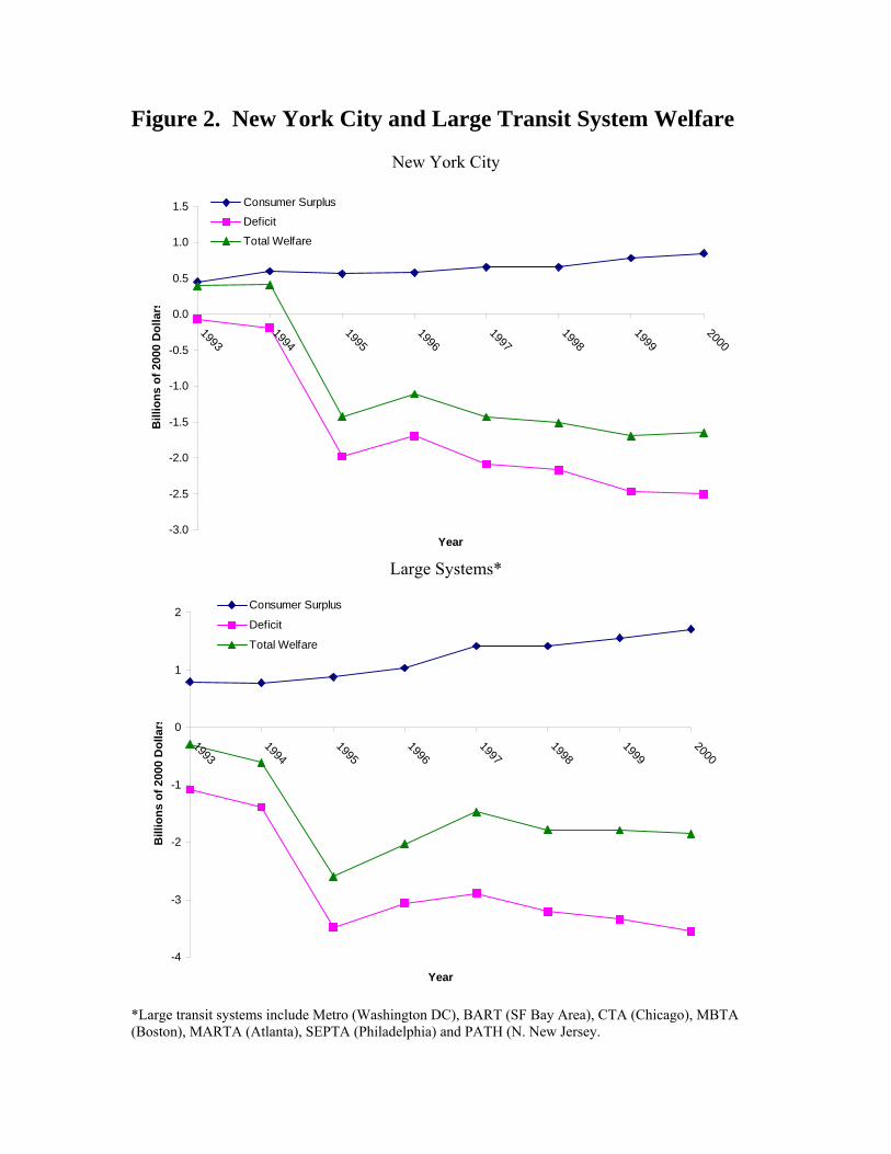
Figure 2. New York City and Large Transit System Welfare

New York City

-3.0

-2.5

-2.0

-1.5

-1.0

-0.5

0.0

0.5

1.0

1.5

19931994

19951996

19971998

19992000

Year

Bill

ions

of 2

000

Dol

lars

Consumer Surplus

Deficit

Total Welfare

Large Systems*

-4

-3

-2

-1

0

1

2

19931994

19951996

19971998

19992000

Year

Bill

ions

of 2

000

Dol

lars

Consumer Surplus

Deficit

Total Welfare

*Large transit systems include Metro (Washington DC), BART (SF Bay Area), CTA (Chicago), MBTA (Boston), MARTA (Atlanta), SEPTA (Philadelphia) and PATH (N. New Jersey.

18

presence of rail transit service in a metropolitan area, measured by its total directional

route miles, reduced the congestion costs incurred by motorists, truckers, and shippers.

We use their estimates for the systems here and present the results in the last two columns

of table 4. Congestion cost savings amount to an additional $2.5 billion in social benefits

and reduce total losses to $4.5 billion, but social net benefits are still negative for all

systems except BART.

In most urban areas it is not surprising that rail transit does not attract enough auto

travelers to be socially desirable, but readers may question that this finding also applies to

New York City. We therefore provide a check on our estimate of the congested-related

benefits from the NYC rail transit system by calculating the congestion costs that would

result if the system were closed. We use a congestion cost function, apparently first

proposed by William Vickery and used in the standard Urban Transportation Planning

Program package provided by the U.S. Department of Transportation to state and local

agencies, which specifies delays as proportional to the fourth power of the traffic volume-

capacity ratio. Based on this function, we find that if all NYC subway users were forced

to use auto travel, congestion costs would increase $1.3 billion (in 2000 dollars). This

figure compares quite favorably as an upper bound to our estimate of $1.2 billion in

congestion costs savings provided by the NYC subways. We note that the cost estimate

is an upper bound because the New York City system is unique among rail transit

systems in its large share, 57 percent, of non-commuters who comprise its ridership

compared with the roughly 20 percent share of non-commuters on other rail systems in

19

the country.26 A greater share of non-commuters who are displaced reduces the costs of

highway congestion because these users have the flexibility to avoid peak-period travel

(Winston and Langer (2005)).

In theory, rail transit could provide additional external benefits besides reducing

roadway congestion, but empirical evidence of these benefits is weak. First, it has been

claimed that by attracting auto users, rail reduces emissions. But given its low load factor

that includes a large share of users who keep older cars to get to suburban rail stations in

large metropolitan areas instead of driving newer cars to get to work and its consumption

of electricity that produces pollution, rail transit does little to improve the environment.27

In addition, the construction and expansion of new and existing rail systems is very

energy intensive. For instance, Tri-County Metropolitan Transit Agency claims that

under the best case scenario, the proposed north light-rail line in Portland, Oregon would

save the equivalent of 7875 gallons of gasoline per day. But the agency also calculates

the energy cost of building the line to be 32 million gallons of gasoline. Thus, even using

the most optimistic estimates, it would take a minimum of 15 years to even begin to

achieve energy savings—and concomitant reductions in emissions—from this rail line.

It has also been argued that rail transit improves the safety of urban travel by

reducing traffic on the road. But motorists absorb (internalize) most of the cost of

accidents through various types of insurance. And the net improvement in safety to those

26 These figures were obtained from the New York City Metropolitan Transit Agency and the 2000 National Transit Database. 27 Mannering and Winston (1991) estimate a duration model of vehicle ownership and find that, all else constant, households who reside in large metropolitan areas hold on to their cars longer than households who reside in smaller metropolitan areas.

20

who switch to rail is small because travelers are still exposed to losses in property and

bodily harm from transit accidents and serious crimes on trains and in stations.28

Finally, it has been suggested that rail has contributed to commercial

development. But case studies have yet to show that after their construction transit

systems have had a significant effect on employment or land use close to stations

(Bollinger and Ihlanfeldt (1997), Charles (2001)).

Notwithstanding the economic efficiency considerations that are unfavorable to

rail transit, supporters of these systems claim they are attractive on distributional grounds

because they contribute to the mobility of low-income residents. But, as noted, the

median income of rail transit users exceeds the median income in the general population.

In addition, rail transit systems have difficulty keeping up with and responding to

changes in job growth; thus, they are unable to provide the poorest residents access to

employment opportunities in outlying suburbs (Winston and Shirley (1998)).

Optimization. Rail transit in its current form does not generate nearly enough

benefits to consumers to offset its massive deficits. However, it is possible that changes

in transit networks, which have not been optimized, could close the gap between benefits

and costs for some systems to the point where they are socially desirable. Using our

demand and cost models, we simulate optimal networks to explore this possibility.

The net benefits produced by transit systems in short-run equilibrium are given by

equation (3). In the long run, it is reasonable to assume that transit agencies can adjust

28 According to calculations from the National Transportation Statistics Report, Bureau of Transportation Statistics 2000, urban fatalities per passenger mile are slightly higher for light rail than for automobile, and comparable for heavy rail and automobile. The small incidence of light rail accidents suggests caution in drawing conclusions from these data. In any case, it is far from clear that rail transit is safer than automobile travel.

21

track length, stations, and so on, which affects demand and costs (assuming the political

impediments to structural network change can be overcome). We therefore optimize the

net-benefits equation with respect to network variables to see if net benefits can

improve.29 For example, we obtain the welfare maximizing level of track by

differentiating net benefits with respect to total track length, assuming the ratio of stations

to track and overall connectivity are held constant. These assumptions allow us to shrink

or expand a transit network while keeping its “shape,” which is influenced by the

physical and geographical characteristics of the city it serves. We find for all systems

that the welfare maximizing level of track is zero (i.e., we obtain corner solutions for all

systems). In other words, no optimal size for any transit system exists that enables it to

generate enough consumer surplus and revenue to offset its short-run total cost. (Our

finding would be even stronger if we performed the optimization using long-run instead

of short-run total cost.)

Another approach to reducing the transit budget deficit would be to raise fares.

Setting prices at marginal cost would produce a three-to fourfold increase in fares for the

vast majority of systems in our sample—an increase that would result in such a massive

attrition of ridership that no improvements in social welfare would be generated.30 Small

29 This analysis considers strategies to improve the net benefits of rail transit systems. We cannot evaluate social net benefits, which account for congestion cost savings to road users, because we do not know how these savings would vary with respect to changes in network variables. It is likely that network optimization would call for reductions in track and stations, which would undoubtedly reduce congestion cost savings to drivers. Hence, our estimate of current congestion savings to drivers serves as an upper bound. 30 Winston and Shirley (1998) found that rail transit use would still fall sharply if fares were raised to marginal cost and if motorists were charged efficient (marginal cost) congestion tolls.

22

increases in fares would have a modest impact on deficits. If neither optimal pricing nor

optimal investment can enable rail systems to generate net benefits, then their social

desirability is clearly in question.

Discussion and Policy Implications

What factors contribute to rail transit’s social undesirability? Rail’s budget

balance is inherently strained by the high costs of building and maintaining a network to

serve urban and suburban travelers and by the inefficiencies associated with low load

factors and excessive labor expenses. Rail is unable to generate revenues to cover these

costs because it must offer low (subsidized) fares to compete with the convenience and

flexibility of autos.

Since the 1970s, deficits expanded as rail costs rose while demand fell. Aging

systems have incurred high costs to repair and maintain their systems. For example, the

Washington Metro has spent nearly $1 billion in recent years to improve system

reliability and ease crowding with little to show for project expenditures.31 The projected

cost of new systems to the public and the federal government has often been

underestimated (or understated) by transit promoters (Pickrell (1990), Flyvbjerg, Holm,

and Buhl (2002)). The public finally rebelled against cost overruns as Los Angeles

county voters in 1998 temporarily halted extensions of their rail system by denying the

use of a county transit sales tax for additional subway projects. But this ballot measure

did not prevent the use of other funds (federal and state) or apply to light rail.

31 Lindsey Layton and Jo Becker, “Efforts to Repair Aging System Compound Metro’s Problems,” Washington Post, June 5, 2005, A1.

23

The demand for rail has continued to shrink because transit networks are unable

to keep up with changing land use and travel patterns that have decentralized residences

and employment. Indeed, less than 10 percent of the nation’s employment in

metropolitan areas is located in old central business districts. Baum-Snow and Kahn

(2005) point out that in cities with rail systems that have not changed their networks,

rail’s share has declined as former patrons and jobs have moved beyond rail’s catchment

areas. Even in cities that have built and expanded their rail systems, persistently

declining population densities in catchment areas have prevented rail from attracting even

a modest (e.g., 2 percent) share of travelers.

Generally, rail cannot be relied on to expand its system in a timely fashion to

attract a potentially large pool of riders when an opportunity exists. For instance, the

Capital Center, located in a suburb outside of Washington DC, was regularly used since

the early 1970s to showcase popular entertainment and professional basketball and

hockey. Metro service to the arena was likely to attract considerable ridership. After

decades of planning and delay, the Metro did open a rail station in 2005 at the site of the

Capital Center—which unfortunately had been demolished three years earlier.

Why do existing systems continue to expand and new systems get built despite

rail’s negative contribution to social welfare? Rail transit enjoys strong support from

urban planners, who wish to discourage auto use, from suppliers of transit capital and

labor, who receive economic rents, from civic boosters, who perceive that a rail system

adds prestige to their city, and from city officials, who support investments in a transit

system that serves the downtown core because it may help the downtown remain vibrant

or keep it from decaying. Until recently, the public has rarely rebelled against the actual

24

costs of new systems or system extensions.32 In fact, opinion polls suggest that a

majority of residents in a city tend to support rail transit regardless of whether they

actually use it on a regular basis.33 We speculate that the public may support rail transit

because it overestimates rail’s ability to mitigate automobile externalities and because it

is “rationally ignorant”—that is, the costs of transit subsidies (relative to other subsidies

in the U.S. economy) are too small to merit the attention of most residents in a

metropolitan area. Facing little resistance from the public, transit advocates aggressively

explore alternative avenues to fund a new system or extend an existing one. And once a

system is built, it is difficult to partially or completely abandon it, so it continues to

receive public support despite its rising welfare costs.34

Rail transit also benefits from substantial congressional support. Title III of the

1982 Surface Transportation Assistance Act granted a “golden penny” to transit (i.e.,

32 As it turns out, the 1998 Los Angeles ballot measure was only a temporary setback for rail transit in LA. In the time since the measure passed a new light rail line has been put into operation, another one is being constructed, and the newly elected mayor, Antonio Villaraigosa, has pledged to extend the Red Line subway along Wilshire Boulevard to the Pacific Ocean. 33 For example, Steven Ginsberg, “Commuters Like Metro More Than They Use It,” Washington Post, March 5, 2005, A1, reports that in a recent Washington Post poll, only 9 percent of Washingtonians said they regularly use the Metro to get to and from work, while two-thirds said that public transportation is not an option for them. However, 58 percent of respondents said they would support more funding for Metro, even if that means higher taxes. 34 Baseball stadiums also enjoy strong public support despite their dubious welfare properties. Indeed, the most successful baseball stadiums, such as Baltimore’s Camden Yards, do not generate enough revenues to justify their substantial costs. In fact, every independent economic analysis of new stadium construction has failed to find measurable positive effects on output or employment, and some analyses have even found negative effects (Zimbalist (2003)). Nonetheless, cities continue to build new stadiums with public funds.

25

transit received one cent of the five cent increase in gasoline taxes). Since then, federal

transportation legislation passed every six years has set aside for transit 20 percent of all

revenues from gasoline tax increases used to rehabilitate and build the nation’s highways

(Dunn (1998)). Congress has therefore solidified rail’s participation in a multimodal

urban transportation system and ensured that its funding will be entwined with highway

funding.35 Recently, rail transit has gained another source of funds through capital

earmarks, which members use to benefit constituents in their districts. In fiscal year

2004, congressional earmarks for new construction and expansion of fixed guideway

capital alone exceeded $1.5 billion (calculated from the Transportation, Treasury, and

Independent Agencies Appropriations Bill Earmarks, 2004).

Could any system be transformed to have a positive effect on social welfare? We

are unable to find ways to significantly raise the net benefits of the nation’s transit

systems given their current operations. However, recently privatized rail transit systems

in foreign cities, most notably Tokyo and Hong Kong, have been able to eliminate

deficits by reducing labor and capital costs and by introducing more comfortable cars and

remote payment mechanisms, among other innovations, that have reduced operating costs

and expanded ridership.

We therefore investigated which, if any, U.S. rail transit systems would become

socially desirable assuming privatization reduced short-run total costs 20 percent—a

plausible estimate based on U.S. and foreign experience with bus transit privatization

(Winston and Shirley (1998)). With the exception of BART, which already generates

35 States have also tied rail funding to highway funding. For example, environmental regulators in Massachusetts ruled that Boston’s “Big Dig” project to depress the central artery could not proceed unless the state expanded Boston’s rail transit system.

26

small net benefits, we found that such a cost reduction would result in only the New York

City and Chicago systems producing positive net benefits.

We are not aware of any public officials who have endorsed complete

privatization of rail transit. On the other hand, a few have encouraged bus transit

agencies to contract with private companies in an effort to reduce costs. Private

contracting would be a politically more feasible alternative to privatization, but it appears

that at best it would enable only a few rail systems to be socially justified.

Because no policy option exists that would enhance the social desirability of most

urban rail transit systems, policymakers only can be advised to limit the social costs of

rail systems by curtailing their expansion. Unfortunately, transit systems have been able

to evolve because their supporters have sold them as an antidote to the social costs

associated with automobile travel, in spite of strong evidence to the contrary.36 As long

as rail transit continues to be erroneously viewed in this light by the public, it will

continue to be an increasing drain on social welfare.

36 Richmond (1998) summarizes the results of interviews he conducted with influential policymakers and residents in Los Angeles, who were convinced that building a rail subway system in the Southland was strongly justified.

27

References

Allgood, Sam and Arthur Snow, “The Marginal Cost of Raising Tax Revenue and Redistributing Income,” Journal of Political Economy, 106, December 1998, pp. 1246-1273. Baum-Snow, Nathaniel and Matthew E. Kahn, “The Effects of Urban Rail Transit Expansions: Evidence from Sixteen Cities, 1970 to 2000,” Brookings-Wharton Papers on Urban Affairs, forthcoming 2005. Baum-Snow, Nathaniel and Matthew E. Kahn, “The Effects of New Public Projects to Expand Urban Rail Transit,” Journal of Public Economics, 77, August 2000, pp. 241-263. Bollinger, Christopher R. and Keith Ihlanfeldt, “The Impact of Rapid Rail Transit

on Economic Development: The Case of Atlanta’s MARTA,” Journal of Urban Economics, 42, September 1997, pp. 179-204.

Charles, John A., “The Mythical World of Transit Oriented Development,” Cascade Policy Institute, Policy Perspective no. 1019, October 2001. Diaz, Roderick B., “Impacts of Rail Transit on Property Values,” American Public Transit Association Rapid Transit Conference Proceedings Paper, May 1999. Dunn, James A., Driving Forces: The Automobile, its Enemies, and the Politics of

Mobility, Brookings Institution, Washington, D.C., 1998. Flyvbjerg, Bent, Mette Skamris Holm, and Soren Buhl, “Underestimating Costs in

Public Works Projects: Error or Lie?,” Journal of the American Planning Association, 68, Summer 2002, pp. 279-295.

Hagget, Peter and Richard J. Chorley, Network Analysis in Geography, St. Martin’s Press, New York, 1969. Kain, John F., “Cost-effective Alternatives to Atlanta’s Rapid Transit System,” Journal of Transport Economics and Policy, 31, January 1997, pp. 25-49. Litman, Todd, “Evaluating Rail Transit Criticism,” Victoria Transport Policy

Institute, October 2004. Mannering, Fred and Clifford Winston, “Brand Loyalty and the Decline of American Automobile Firms, Brookings Papers on Economic Activity: Microeconomics, 1991, pp. 67-114. Pickrell, Don, Urban Rail Transit Projects: Forecast Versus Actual Ridership and Costs, U.S. Department of Transportation, Washington, D.C., 1990.

28

Pozdena, Randall J. and Leonard Merewitz, “Estimating Cost Functions for Rail

Rapid Transit Properties,” Transportation Research, 12, April 1978, pp. 73-78. Richmond, Jonathan, “A Whole-System Approach to Evaluating Urban Transit Investments,” Transport Reviews, 21, 2001, pp. 141-179. Richmond, Jonathan, “The Mythical Conception of Rail Transit in Los Angeles,” Journal of Architectural and Planning Research, 15, 1998, pp. 294-320. Savage, Ian, “Management Objectives and the Causes of Mass Transit Deficits,” Transportation Research, 38A, 2004, pp. 181-199. Savage, Ian, “Scale Economies in United States Rail Transit Systems,”

Transportation Research, 31A, 1997, pp. 459-473. Savage, Ian and August Schupp, “Evaluating Transit Subsidies in Chicago,” Journal of

Public Transportation, 1, Winter 1997, pp. 93-117. Small, Kenneth A. Urban Transportation Economics, Harwood Academic Publishers, Chur, Switzerland, 1992. Viton, Philip A., “On Competition and Product Differentiation in Urban

Transportation: The San Francisco Bay Area,” Bell Journal of Economics, 12, Autumn 1981, pp. 362-379.

Viton, Philip A., “On the Economics of Rapid-Transit Operations,” Transportation Research, 14A, 1980, pp. 247-253. Voith, Richard,“The Long-Run Elasticity of Demand for Commuter Rail Transportation,” Journal of Urban Economics, 30, November 1991, pp. 360-372. Winston, Clifford, “Conceptual Developments in the Economics of Transportation:

An Interpretive Survey,” Journal of Economic Literature, 23, March 1985, pp. 57-94.

Winston, Clifford and Ashley Langer, “The Effect of Government Spending on

Road Users’ Congestion Costs,” Brookings Institution working paper, April 2005. Winston, Clifford and Chad Shirley, Alternate Route: Toward Efficient Urban Transportation, Brookings Institution, Washington, D.C., 1998. Zimbalist, Andrew, May the Best Team Win: Baseball Economics and Public Policy,

Brookings Institution, Washington, D.C., 2003.