Pluto’s global surface composition through

pixel-by-pixel Hapke modeling of New Horizons

Ralph/LEISA data

S. Protopapaa, W. M. Grundyb, D.C. Reuterc, D.P. Hamiltona, C. M. DalleOred,e, J.C. Cookf, D.P. Cruikshanke, B. Schmittg, S. Philippeg, E.

Quiricog, R. P. Binzelh, A.M. Earleh, K. Ennicof, C.J.A. Howettf, A.W.Lunsfordc, C. B. Olkinf, A. Parkerf, K.N. Singerf, A. Sternf, A. J.

Verbiscerj, H. A. Weaveri, L.A. Youngf, the New Horizons Science Team

aUniversity of Maryland, Department of Astronomy, College Park, Maryland 20742,USA

bLowell Observatory, Flagstaff, Arizona 86001, USAcNational Aeronautics and Space Administration Goddard Space Flight Center,

Greenbelt, Maryland 20771, USAdSETI Institute

eNASA Ames Research CenterfSouthwest Research Institute, Boulder, Colorado 80302, USA

gInstitut de Planetologie et Astrophysique de Grenoble, UGA / CNRS, IPAG, GrenobleCedex 9, France

hMassachusetts Institute of TechnologyiJohns Hopkins University Applied Physics Laboratory

jUniversity of Virginia

Abstract

On July 14th 2015, NASA’s New Horizons mission gave us an unprecedented

detailed view of the Pluto system. The complex compositional diversity of

Pluto’s encounter hemisphere was revealed by the Ralph/LEISA infrared

spectrometer on board of New Horizons. We present compositional maps of

Pluto defining the spatial distribution of the abundance and textural prop-

erties of the volatiles methane and nitrogen ices and non-volatiles water ice

and tholin. These results are obtained by applying a pixel-by-pixel Hapke

Preprint submitted to Icarus December 1, 2016

arX

iv:1

604.

0846

8v2

[as

tro-

ph.E

P] 3

0 N

ov 2

016

radiative transfer model to the LEISA scans. Our analysis focuses mainly on

the large scale latitudinal variations of methane and nitrogen ices and aims

at setting observational constraints to volatile transport models. Specifi-

cally, we find three latitudinal bands: the first, enriched in methane, extends

from the pole to 55◦N, the second dominated by nitrogen, continues south to

35◦N, and the third, composed again mainly of methane, reaches 20◦N. We

demonstrate that the distribution of volatiles across these surface units can

be explained by differences in insolation over the past few decades. The lat-

itudinal pattern is broken by Sputnik Planitia, a large reservoir of volatiles,

with nitrogen playing the most important role. The physical properties of

methane and nitrogen in this region are suggestive of the presence of a cold

trap or possible volatile stratification. Furthermore our modeling results

point to a possible sublimation transport of nitrogen from the northwest

edge of Sputnik Planitia toward the south.

Keywords: Pluto, surface; Ices, IR spectroscopy; Radiative transfer

1. Introduction

NASA’s New Horizons mission completed a close approach to the Pluto

system on 14 July 2015 reaching a distance of 12,000 km from the dwarf

planet’s surface (Stern et al., 2015). A wealth of ground-based data of the

Pluto system had been collected prior to the New Horizons mission, moti-

vated first by its status as the outermost planet and later by its being among

the few trans-Neptunian objects (TNOs) bright enough for detailed studies

to further advance our knowledge of the Kuiper Belt.

The synergy of ground-based observations, modeling efforts and labora-

2

tory studies have highlighted over the course of the past years, among other

things, 1) the presence of methane (CH4), nitrogen (N2), carbon monoxide

(CO) and ethane (C2H6) ices on Pluto together with tholins, 2) constraints

on Pluto’s surface temperature, and 3) the state of CH4 ice. CH4, N2, and CO

ices were detected through ground-based measurements in the near-infrared

wavelength range (Cruikshank et al., 1976; Owen et al., 1993). While CH4 is

the most spectroscopically active constituent among Pluto’s ices, with several

strong absorption bands, CO and N2 were identified by the detection of the

bands at 2.35 µm, as well as the weaker band at 1.58 µm, and 2.15 µm, re-

spectively. Models of Pluto’s near-infrared reflectance spectra including C2H6

yield an improved reduced χ2, leading to the conclusion that this ice is also

present on the surface of the planet (DeMeo et al., 2010; Holler et al., 2014;

Merlin, 2015). The red slope of Pluto’s continuum (Bell et al., 1979; Grundy

and Fink, 1996; Lorenzi et al., 2016) observed from the visible to around

∼1 µm has been attributed to the presence of organic materials on the sur-

face of the body, such as tholins. These are the refractory residues obtained

from the irradiation of gases and ices containing hydrocarbons (Cruikshank

et al., 2005). In the case of Pluto, tholins may form in situ through energetic

processing of CH4 and N2 ices (Cruikshank et al., 2016). The spectral profile

of the 2.15-µm N2 absorption band is temperature dependent (Grundy et al.,

1993; Tryka et al., 1993) and transitions from broad to very narrow according

to whether N2 is in the hexagonal β- (above 35.6 K) or cubic α-phase, respec-

tively. Tryka et al. (1994), using N2 as a spectral ‘thermometer’, inferred a

surface temperature of 40±2 K. At such temperature, thermodynamic equi-

librium dictates that pure CH4 ice cannot co-exist with pure N2 ice. If both

3

species are present, then instead of pure ices the phases are (Trafton, 2015):

CH4 saturated with N2 (CH4:N2) and N2 saturated with CH4 (N2:CH4).

The solubility limits of CH4 and N2 in each other are temperature dependent

and are equal to about 5% (N2:CH4, with 5% CH4) and 3% (CH4:N2 with

3% N2) at 40 K (Prokhvatilov and Yantsevich, 1983). CH4 when dissolved in

N2 presents absorption bands shifted toward shorter wavelengths compared

to the central wavelengths of pure CH4 (Quirico and Schmitt, 1997; Grundy

et al., 2002). This shift, which is wavelength dependent and is observed in

Pluto spectra (Owen et al., 1993), varies with the CH4 abundance in the

mixture: the larger the CH4 concentration the smaller the blueshift (Schmitt

and Quirico, 1992; Quirico and Schmitt, 1997; Protopapa et al., 2015).

While ground-based measurements have played a remarkable role in the

growth of knowledge about Pluto’s composition (Cruikshank et al., 2015a),

they were limited in providing composition maps of Pluto. From the ground,

it is possible to investigate changes of Pluto surface composition with lon-

gitude by comparing measurements obtained at different rotational phases.

Variations with latitude can be determined only by monitoring Pluto as it

moves around the Sun during the 248 year orbit. However, over time scales

of years, Pluto might undergo a resurfacing process (Stern et al., 1988; Buie

et al., 2010a,b). N2, CO, and CH4 ices are all volatiles at Pluto surface

temperature, of which CH4 is the least volatile, and support Pluto’s atmo-

sphere. Changes in insolation over the course of a Pluto’s orbit can result in

the bulk migration of volatile ices (Spencer et al., 1997; Hansen and Paige,

1996; Young, 2012, 2013; Hansen et al., 2015). It is therefore difficult to

disentangle temporal and spatial variations using ground-based observations

4

(Grundy et al., 2013, 2014).

New Horizons provided a detailed snapshot of the Pluto system with the

goal, among others, to map Pluto surface composition and search for addi-

tional surface species (Young et al., 2008). New Horizons confirmed the pres-

ence on Pluto surface of the volatile ices N2, CH4, and CO and detected the

existence of the non-volatile water (H2O) and possibly methanol (CH3OH)

ices (Grundy et al., 2016; Cook et al., 2016). The detection of H2O-ice did

not come as a surprise given that most TNOs are characterized by H2O-

ice dominated spectra (Barucci et al., 2008). Furthermore, Triton, which is

thought to be a former TNO captured into a retrograde orbit around Nep-

tune (Agnor and Hamilton, 2006), presents a near-infrared spectrum similar

to that of Pluto with clear evidence of H2O-ice absorption bands (Quirico

et al., 1999; Cruikshank et al., 2000). Contrary to Triton (Cruikshank et al.,

1993), Pluto does not display the signatures of carbon dioxide (CO2) ice on

the surface (Grundy et al., 2016).

New Horizons revealed striking variations in the distribution of Pluto’s

ices (Grundy et al., 2016). These results rely on the analysis of spectral

parameters, including band depth and equivalent width. However, the main

limitation of that approach is the incapability of disentangling relative abun-

dance from grain size effects. This is possible only by means of radiative

transfer modeling of the absorption bands over a wide wavelength range,

a method that has its own limitations (see Section 5). In this paper, we

will discuss constraints on the abundances and scattering properties of the

materials across the surface of Pluto, focusing mainly on the distribution

of N2 and CH4 ices and the relation between their distribution and surface

5

geology, which is vital to set observational constraints for volatile transport

models (Young, 2013; Hansen et al., 2015; Bertrand and Forget, 2016).

2. Observations

Spatially resolved near-infrared spectra of Pluto’s surface were acquired

using the Linear Etalon Imaging Spectral Array (LEISA), part of the New

Horizons Ralph instrument (Reuter et al., 2008). LEISA consists of a wedged

filter placed in close proximity to a 256×256 pixels detector array. The fil-

ter consists of two segments covering the wavelength range 1.25-2.5 µm and

2.1-2.25 µm at the resolving power (λ/∆λ) of 240 and 560, respectively.

The low-resolution 1.25-2.5 µm segment is used to infer the surface compo-

sition of Pluto as outer solar system ices such as N2, CH4, H2O have strong

unique absorption bands in this wavelength region. The high-resolution 2.1-

2.25 µm segment is instead sensitive to the spectral shape of the 2.15-µm ab-

sorption band of N2 ice, which is temperature dependent, as well as to the

spectral shape and position of the 2.2-µm absorption band of CH4 ice, which

is important to assess the CH4 to N2 mixing ratio. The wavelength varies

along the row direction of the detector array. LEISA is operated in a scan-

ning mode. A series of image frames, N , are acquired while scanning the field

of view across the target surface in a push broom fashion. The target moves

through the image plane, along the spectral direction, also called along-track

direction. A process of co-registration of each wavelength image is applied,

removing motion and optical distortions, to obtain a three-dimensional ar-

ray spectral cube where each frame images the target surface at a distinct

LEISA wavelength. The same process of co-registration is applied to gen-

6

erate a wavelength spectral cube, such that each pixel has its own spectral

array. This way we take into account an existing spectral distortion (‘smile’)

of 2-3 spectral elements along the 256 scanning cross-track pixels due to a

slight curvature induced by the filter deposition process.

In this paper we present two LEISA resolved scans of Pluto collected

at a distance from Pluto’s center of ∼100,000 km at a spatial scale of 6

and 7 km/pixel (see Table 1 for details). The LEISA data presented here

have been calibrated through the most up-to-date pipeline processing, which

includes bad pixel masking, flat fielding, and conversion from DN to radiance

I expressed in erg s−1cm−2A−1str−1. The latter is normalized by the incoming

solar flux to obtain reflectance (I/F ). Efforts to improve the radiometric

calibration and flat-field are currently underway. Improvements will probably

be made as more spectral data from Pluto and Charon are downlinked and

become available. The possible impact of calibration changes have been

considered in the results presented here.

The last step in the data processing consists of determining the Pluto

latitude and longitude corresponding to each LEISA pixel. Integrated Soft-

ware for Imagers and Spectrometers (ISIS, https://isis.astrogeology.

usgs.gov/) provided by the United States Geological Survey (USGS) uses

the spacecraft attitude history, which is measured and recorded as part of the

standard housekeeping data, along with its LEISA camera model and the re-

constructed spacecraft trajectory to determine where each LEISA pixel falls

on the target body. We used the ISIS software to perform an orthographic

projection of the LEISA data to a sphere at the target’s size and location rel-

ative to the spacecraft as of the mid-time of each scan. The two LEISA scans

7

presented in this paper combined cover Pluto’s full disk and they were both

projected to a common orthographic viewing geometry appropriate for the

mid-time between the two. The re-projection was done to a target grid with

a spatial scale of 2 km/pixel, a higher resolution than the native LEISA pixel

scales (see Table 1). The point of sub-sampling is to minimize degradation

of spatial information as a result of the nearest neighbor re-sampling. Using

the ISIS “translate” routine, we applied a global shift of the LEISA data

(consistent across all LEISA wavelengths) to correct for a few pixels mis-

match between the LEISA cube and the much higher resolution base map

obtained with the Long Range Reconnaissance Imager (LORRI, Cheng et al.,

2008) projected to the same geometry. We took into account higher order

corrections by means of the ISIS “warp” routine. This is based on a user

supplied control network constructed using features that were recognizable

in both LEISA and LORRI data. These corrections resulted in LEISA cubes

estimated to be geometrically accurate to a little better that a single LEISA

pixel. The mid-scan geometry was taken as a reasonable approximation of

the illumination and viewing geometry for each pixel.

The modeling analysis presented in this paper is conducted on the LEISA

scans degraded to a spatial resolution of∼12 km/pixel through bin averaging.

The mean absolute deviation of the incident and emergent angles within a

bin is generally less than ∼0.2 deg but at the limb where it approaches ∼1

deg. The two scans overlap in a region crossing Elliot Crater1 and Sputnik

Planitia. To assess the error in the I/F data introduced by variations in the

1All place names used in this paper are informal designations

8

Table 1: Details of the LEISA scans presented in this paper.Request ID P LEISA Alice 2a P LEISA Alice 2b

MET 299171897 299172767

S/C Start Time, UTC 2015-07-14 2015-07-14

09:26:19 09:40:49

Phase [deg] 21.7 22.4

SubSol Lat [deg] 51.6 51.6

SubSol Lon [deg] 133.4 132.9

SubS/C Lat [deg] 38.8 38.2

SubS/C Lon [deg] 158.6 158.7

Spatial Scale [km/px] 7 6

quality of the flat-field, scattered light, and other spatially correlated noise

sources, we compared the two scans in the region of overlap. A variety of

statistical comparisons all consistently produce a conservative estimate of 5%

as the mean 1σ uncertainty contributed by these sources of error.

3. Spectral Modeling

The goal of our analysis is to understand the spatial distribution of the

abundance and textural properties of each Pluto’s surface component. To

this end we performed a pixel-by-pixel modeling analysis of the LEISA spec-

tral cubes. This approach requires the application of the same modeling

strategy across the entire visible face of Pluto, so that a systematic and com-

parative study between the composition of the different surface units can be

conducted. This is at the expense of possible compositional peculiarities in

small surface areas.

We now describe the modeling of a single pixel LEISA spectrum. We

use the scattering radiative transfer model of Hapke (1993) to compute the

9

bidirectional reflectance r of a particulate surface as

r(i, e, g) =w

4π

µ0e

µe + µ0e

{[1 +B(g)]P (g)+

H(µe)H(µ0e)− 1}S(i, e, g). (1)

The single scattering albedo w is the ratio of the scattering efficiency to

the extinction efficiency (w = 0 implies that the particles absorb all the

radiation) and it can be computed only if the optical constants n and k, the

real and imaginary part of the refractive index, respectively, of the surface

component, as a function of the wavelength λ, are known. We adopt the

equivalent slab model presented by Hapke (1993) to compute w, given the

complex refractive index. Notice that w is a function of the particle’s effective

diameter D, which is a free parameter in our analysis. The terms µ0e and

µe are related to the cosine of the incidence angle (i) and emission angle

(e), respectively, with additional terms to account for the tilt of the surface,

due to surface roughness. The latter is also accounted for by the shadowing

function S(i, e, g), which involves the mean slope angle θ. The backscatter

function B(g) is an approximate expression for the opposition effect and it

is given by

B(g) =B0

1 + (1/h) tan(g/2), (2)

where g is the phase angle, h is the compaction parameter and character-

izes the width of the nonlinear increase in the reflectance phase curve with

decreasing phase angle (the opposition surge), and B0 is an empirical factor

that represents the amplitude of the opposition effect. We adopt for P (g) a

single lobe Henyey and Greenstein function

P (g) =1− ξ 2

(1 + 2 ξ cos g + ξ2)3/2, (3)

10

where ξ is the cosine asymmetry factor. The Ambartsumian–Chandrasekhar

H-functions are computed using the approximation proposed by Hapke (2002).

Equation (1) can be used to compute the bidirectional reflectance of a

medium composed of closely packed particles of a single component. How-

ever, the surface of interest is a mixture of different constituents (Grundy

et al., 2016). Even at the pixel level, more than one component can be

present. Therefore, in order to calculate synthetic reflectance spectra for

comparison with the observational data, it is necessary to compute the re-

flectance of a mixture of different types of particles. We have considered

an areal (also called geographical) mixture, which consists of materials of

different composition and/or microphysical properties that are spatially iso-

lated from one another. We adopt this approach as it is the most simple

and it provides satisfactory results. In the case of areal mixture, the bidirec-

tional reflectance spectra of the individual components (ri) are summed with

weights equal to the fractional area of each terrain (Fi), as shown below

r =∑i

Firi where∑

i Fi = 1. (4)

By considering an areal mixture, we are implying that there is no multiple

scattering between different components. Given the definition of bidirectional

reflectance by Hapke (1993) as the ratio between the radiance at the detector

and the irradiance incident on the medium, we have that I/F = πr. We

set the cosine asymmetry parameter ξ = −0.3, the compaction parameter

h = 0.5, the amplitude of the opposition effect B0 = 1, and mean roughness

slope θ = 10◦, following previous studies (Olkin et al., 2007; Buie et al.,

2010b).

11

The free parameters in our model are effective diameter (Di) and con-

tribution of each surface terrain to the mixture (Fi) . They are iteratively

modified by means of a Levenberg-Marquardt χ2 minimization algorithm

until a best-fit to the observations is achieved.

It is possible to determine a spatial map for the abundance and grain size

of each surface material by applying the modeling analysis described above

pixel-by-pixel. Notice that we consider the other Hapke parameters to be

constant across Pluto’s surface.

4. Mixture endmembers

The surface components considered in the mixture are H2O ice, N2:CH4 ice,

CH4:N2 ice, and Titan tholin. The choice of the surface terrain units relies

on the spectral evidence collected over the course of several years, which are

outlined in Section 1. For details about the optical constants used for each

surface material see Table 2 and the following discussion.

4.1. Tholins

While there is no doubt about the presence of tholins on the surface

of Pluto, the specific type of organic material responsible for Pluto’s color,

ranging from yellow to red (Stern et al., 2015; Grundy et al., 2016), is still

unknown. Different types of tholins have been studied but there are only a

few for which optical constants are available (for a review on the different

kind of tholins the reader is refereed to de Bergh et al., 2008). In particular,

the most common are Triton tholin and Titan tholin, which are obtained

by irradiating gaseous mixtures of N2 and CH4. The difference between the

two is in the initial N2 to CH4 gaseous mixing ratio (McDonald et al., 1994;

12

Table 2: Optical constantsMaterial Source Temperature Filename Wavelength range Notes

[K] [µm]

Titan Tholin Khare et al. (1984) 0.02–920.0

CH4-ice Grundy et al. (2002)1 39 optcte-Vis+NIR+MIR-CH4cr-I-39K 0.7–5.0

N2-ice Grundy et al. (1993)1 36.5 optcte-NIR-beta-N2-36.5K 2.062–4.762 N2 is in β-phase. We

set n = 1.23 and k =

0, below 2.1 µm.

N2:CH4-ice Quirico and Schmitt (1997)1 36.5 optcte-NIR-CH4-lowC-beta-N2-36.5K 1–5 β-N2:CH4 solid solu-

tion with CH4 con-

centrations lower than

2%. The absorption

coefficient of diluted

CH4 is normalized to

a concentration of 1.

H2O-ice Grundy and Schmitt (1998)1 40 0.96-2.74

1Optical constants are available at http://ghosst.osug.fr/.

Cruikshank et al., 2005; de Bergh et al., 2008). Spectrally, both types of

tholins present a red slope in the visible, but Triton tholin contrary to Titan

tholin also displays a red slope in the near-IR. Laboratory measurements

are currently underway to obtain refractory tholins particularly relevant to

Pluto (Pluto’s ice tholin) through UV and low-energy electron bombardment

of a mixture of Pluto’s ices (N2:CH4:CO = 100:1:1, Materese et al., 2015).

A preliminary reflectance spectrum of Pluto’s ice tholin has been presented

by Cruikshank et al. (2015b, 2016), but no optical constants are available

at this time. The spectrum shows a red slope between 0.5 and 1 µm, and

turns blue in the range between 1 and 2.5 µm. We adopt Titan tholin in the

modeling (see Table 2), given the similar spectroscopic behavior with respect

to Pluto’s ice tholin. The choice of Titan instead of Triton tholin is further

13

1.6 1.8 2.0 2.2 2.4Wavelength (µm)

10−10

10−8

10−6

10−4

10−2

Imagin

ary

part

of th

e r

efr

active index k

http://ghosst.osug.fr/Protopapa et al. 2015pure CH4

see text for detailsProtopapa et al. 20155% CH4 in N2

Figure 1: The comparison between the imaginary part of the refractive index, k, of a

N2:CH4 mixture with 5% CH4 in N2 computed numerically (black line, see text for details)

and measured in the laboratory by Protopapa et al. (2015, blue dots) is shown. For

reference, two sets of k for pure CH4 at similar temperatures (gray dashed line and red

dots) are shown.

supported by the blue slope of the Pluto/LEISA spectra extracted in the

area informally known as Cthulhu Regio, which is a large, dark region along

Pluto’s equator and one of the darkest and reddest regions on the surface,

at visible wavelengths. However, we emphasize that the search for the most

appropriate tholin continues and is not the goal of this preliminary study.

4.2. N2-rich and CH4-rich saturated solid solutions

Protopapa et al. (2015) present optical constants for solid solutions of

methane diluted in nitrogen (N2:CH4) and nitrogen diluted in methane (CH4:N2)

at temperatures between 36 and 90 K, at different mixing ratios http:

//www2.lowell.edu/users/grundy/abstracts/2015.CH4+N2.html. This

set of measurements, which includes optical constants of N2-rich (N2:CH4)

14

and CH4-rich (CH4:N2) saturated solid solutions, cover the same wave-

length range as the LEISA spectrometer. However, they are available in

narrow blocks of wavelengths covering regions of intermediate absorption

only. This implies that no optical constants are available for N2:CH4 and

CH4:N2 around 1.5 and 2.0 µm, where water ice, which turned out to be

an undisputed component on the surface of Pluto, presents diagnostic ab-

sorption features. While further efforts are being conducted to complete this

data set, we adopt optical constants of pure CH4 as a proxy for CH4:N2 and

generate optical constants for N2:CH4 following the method described by

Doute et al. (1999).

The solubility limit of N2 in CH4 is 3% at 40K. The wavelength shift of

the CH4 bands in such a system is smaller than the LEISA resolving power –

shifts on the order of ∼2×10−4 µm are reported by Protopapa et al. (2015),

which is over an order of magnitude smaller than the LEISA resolution.

Therefore, we do not expect our analysis to be significantly affected by the use

of pure CH4 in place of CH4:N2. This is still valid at temperatures lower than

40 K, as the solubility limit of N2 in CH4 decreases with decreasing tempera-

tures (see the CH4-N2 binary phase diagram by Prokhvatilov and Yantsevich,

1983) and smaller shifts correspond to higher CH4 abundances. We use the

optical constants of crystalline CH4-I at 39 K from http://ghosst.osug.fr/

(see Table 2 for details). We follow the method described by Doute et al.

(1999) to numerically generate optical constants for N2:CH4. We consider

two reference components: the first one is identified with pure N2 ice, and

the second is CH4 initially diluted in the nitrogen matrix, but artificially

normalized to unit concentration (Quirico et al., 1999). Doute et al. (1999)

15

assume that, for each wavelength, the scalar product of the complex indices

of N2 and the diluted CH4 by the vector

[1-FCH4

N2:CH4, FCH4

N2:CH4

]gives the

optical constants of a mixture with a percentage of CH4 in solid N2 equal

to FCH4

N2:CH4. We validate this numerical approach against the optical con-

stants measured by Protopapa et al. (2015) for FCH4

N2:CH4=5%, which is the

solubility limit of CH4 in N2 at 40 K. We use the optical constants for pure

N2 and N2:CH4 listed in Table 2. As shown in Figure 1, the numerical ap-

proach (black line) well reproduces not only the strengths of the measured

(blue dots) CH4 bands but also that of N2 at 2.15 µm. The concentration of

CH4 in N2 (FCH4

N2:CH4) is a free parameter in our study.

4.3. H2O-ice

Laboratory measurements show that infrared water ice absorption bands

at 1.5, 1.65 and 2.0 µm change position and shape as a function of phase

(crystalline or amorphous) and temperature (Grundy and Schmitt, 1998).

We do not solve in this analysis for H2O-ice temperature and phase and use

instead optical constants of crystalline hexagonal water ice at 40 K (see Ta-

ble 2, http://www2.lowell.edu/users/grundy/abstracts/1998.H2Oice.

html).

5. Model discussion

Applying the pixel-by-pixel modeling analysis described in Section 3 is

highly computationally expensive. To overcome such limitation, we have

implemented our code with multi-threading capabilities. The main code

splits the modeling of different surface units across Pluto between multiple

16

threads of execution. We run our simulations on a multi-processor machine

where these threads can execute concurrently. Furthermore, to speed up

the task, the pixel-by-pixel modeling analysis is applied to the LEISA data

degraded to a spatial resolution of ∼12 km/pixel (for a total of ∼4×104 pixels

to model). Using 15 threads, the modeling of each LEISA scan requires

approximately 10 hours.

We present results obtained by applying the Hapke radiative transfer

model, assuming an areal mixture of the single endmembers. Several scat-

tering theories (e.g., Shkuratov et al., 1999; Doute and Schmitt, 1998) as

well as different types of mixtures (e.g., intimate) exist. These alternative

methods could possibly provide similar quality of fits to the data as those

presented here but with different percentages and grain size of the compo-

nents (Poulet et al., 2002). However, we decided to interpret the Pluto New

Horizons data with a simple model since it provides a reasonable fit to all

104 Pluto spectra (see Section 6). The one presented here is an automated

process and a perfect match between observations and the model is beyond

the scope of the analysis. Ultimately, the goal is to perform a comparative

study between Pluto’s main surface units, which can only be done when the

same modeling strategy is applied successfully to the full surface of Pluto.

As noted by Barucci et al. (2008), grain size and abundance are sometimes

entangled. This occurs mainly when the absolute I/F is unknown and when

the analysis is not conducted over a wide wavelength range, which fortunately

is not the case for the New Horizons data. We acknowledge that this problem

could still arise in absence of defined absorption bands, as in some areas

dominated by non-volatile components.

17

The estimates of the concentration and particle size of each surface com-

pound rely on the choice of the Hapke parameters ξ, h, B0, and θ, since these

surface photometric properties affect the entire reflectance spectrum. As dis-

cussed in Section 3, we treat these properties as global quantities, constant

across all of Pluto’s terrains. Given the high degree of surface variations on

Pluto, this approximation may not be correct. Work is ongoing to determine

the values of these parameters across Pluto’s main surface units by inverting

the New Horizons Multi-spectral Visible Imaging Camera (MVIC; Reuter

et al., 2008) data acquired at different phase angles (Buie et al., 2016). Our

analysis will be revisited when the problem of Pluto’s photometric properties

will be unraveled, which may take some time given its complexity.

While New Horizons confirmed the detection of CO ice on Pluto’s sur-

face, mainly in Sputnik Planitia (Grundy et al., 2016), we did not include this

component in our models. The main reason is the lack of optical constants in

the continuum region, outside of the CO ice absorption bands. Assumptions

on the absorption coefficient of CO ice in the continuum region would affect

the determination of the abundance and grain size of the other surface com-

pounds, for which optical constants are instead known. We will investigate

the inclusion of CO ice in our models as well as other minor species like C2H6

in future work.

6. Results

We discuss below the spatial distribution of the abundance and grain size

of non-volatiles and volatiles.

18

6.1. Non-Volatiles

Locations enriched in Titan tholin and H2O ice are correlated with specific

geologic regions (see panels B and D of Figure 2, e.g., Cthulhu Regio, Bare

Montes, Piri Planitia, Inanna Fossa, Moore et al., 2016). A change in H2O-

ice abundance and grain size (panels B and C of Figure 2) is observed across

these different terrains. In Figure 2 areas of interest are labelled and their

corresponding spectra (blue points, with 1σ error estimates), compared with

the best fit modeling (red line), are displayed in Figure 3. The spectra are

arranged in decreasing H2O-ice abundance from top to bottom.

The region in the vicinity of Pulfrich crater (region “a”) stands out for

being particularly enriched in H2O ice, with abundances close to 60% (see

Table 3). The enrichment of H2O ice in the vicinity of Pulfrich crater is

in good agreement with the map displaying the correlation coefficient be-

tween each LEISA spectrum and a template Charon-like H2O ice spectrum

(Grundy et al., 2016; Cook et al., 2016). The spectrum extracted in this re-

gion (panel “a”, Figure 3) shows indeed strong diagnostic absorption bands

due to H2O ice at 1.5 and 2.0 µm, including the 1.65-µm feature, which is

characteristic of the crystalline phase of the H2O ice (Grundy and Schmitt,

1998). The relative strength and shape of the H2O-ice absorption bands are

consistent with grain sizes on the order of ∼150 µm. Notice that the best

fit modeling suggests the presence not only of H2O ice but also of tholin and

CH4. The latter produces the absorption bands beyond 2.2 µm. Differences

between observations and modeling around 1.4 and 1.7 µm are attributed

to flat-fielding, which still requires further optimization. We conclude that

across Pluto’s encounter hemisphere, no regions of 100% H2O ice are ob-

19

served, at this spatial resolution.

The spectrum extracted along Virgil Fossae (region “b”) displays a spec-

tral behavior, including the absolute value of I/F , similar to that of Pulfrich

crater but with shallower H2O-ice absorptions. The comparison of the mod-

eling parameters obtained for these two terrains highlights the importance of

radiative transfer modeling of the absorption bands to disentangle the effects

of grain size, abundance and illumination geometry (see Table 3). The qual-

itative comparison between these two spectra (“a” and “b”) would lead to

the conclusion that the fractional abundance of H2O ice is higher in Pulfrich

crater than in Virgil Fossa. While this is still the case, a difference in the

particle diameter of H2O ice is also observed. This is required to take into ac-

count the variation in illumination geometry, which plays as important a role

as composition and texture in determining the observed spectral properties

of the surface.

The spectrum extracted in the Cthulhu Regio (region “c”) presents, with

respect to the two spectra discussed above, shallower H2O-ice absorption

bands and a neutral spectral slope. This is consistent with smaller H2O-

ice particle diameters (∼10 µm). Furthermore, the absolute value of I/F is

lower (on the order of 0.4 instead of 0.6), consistent with a higher abundance

of tholins. The spectral effect of tholins is indeed to darken the albedo

level, without introducing any significant spectral features. Notice that the

absolute I/F values of Titan tholin decrease with increasing grain size. This

explains our modeling results, which show regions across Pluto with lower

reflectance values (e.g., Cthulhu Regio) corresponding to higher abundances

of tholin and larger particle diameters (panels D and E in Figure 2).

20

A few areas across Hayabusa Terra (e.g., region “d”) exhibit evidence of

H2O ice. The strong CH4 absorption features not only beyond 2.2 µm but

also across the full wavelength range are indicative of a greater contribution

of this ice compared to the previously described regions. At the same time,

the presence of H2O ice is highlighted by the depression in the spectral region

around 2.0 µm. These features would not be evident in a spectrum mainly

dominated by methane ice, as in the case displayed in panel “e” of Figure 3. It

is important to point out that spectra from near the north pole and from most

of Tombaugh Regio do not show any spectral evidence for the presence of

H2O ice. On the other hand, the modeling results indicate abundances on the

order of 10% and corresponding grain sizes larger than 1000 µm. Synthetic

spectra of H2O ice with such large particles present saturated bands and very

low reflectance values. Therefore we infer that water ice in this case is a filling

material, spuriously adopted by the modeling code. This is supported by the

fact that the model of region “e” with null H2O ice abundance, provides

an equally good fit (comparable χ2) to the one presented in Figure 2. The

absence of H2O ice mainly affects the grain size and abundance of the tholins,

which in this instance have larger values than those reported in Table 3 for

case “e”. Analogously, the contribution of N2:CH4 in all cases where its

abundance is lower than 10% is considered not significant.

6.2. Volatiles

No major region across Pluto’s surface is completely depleted of CH4 (panel

A, Figure 4). N2 on the other hand presents a more localized distribution

(panel A, Figure 5). We identify in the volatile maps large scale latitudinal

regions, which differ in abundance and texture of the CH4-rich and N2-rich

21

components.

The first of these terrains is Lowell Regio, labelled “f” (Figure 4-5). The

second is the belt stretching from latitude 35◦N to 55◦N and crossing Burney

Crater and Hayabusa Terra (identified with “g” in Figure 4 and 5). This belt

appears to be interrupted by Sputnik Planitia, a deep reservoir of convecting

ices (McKinnon et al., 2016a,b; Trowbridge et al., 2016). The relative amount

of the CH4-to-N2-rich components decreases with decreasing latitude. This

is demonstrated by the spectra extracted from representative locations in

these two surface units (Figure 6). Spectrum “f”, contrary to its counterpart

“g”, does not display a N2-absorption feature at ∼2.15 µm (vertical dashed

line). The modeling indicates a N2 distribution on the order of 30% and 45%

across Lowell Regio and between 35◦N and 55◦N, respectively (see Table 3).

Notice that the presence of an N2-rich component is marked not only by the

∼2.15 µm absorption band but also by the absolute level of the continuum,

being higher where N2 occurs. Furthermore a difference in the path length

Table 3: ModelsRegion geometry H2O Titan tholin CH4:N2 N2:CH4 FCH4

N2:CH4χ2

i[deg] e[deg] F[%] D[µm] F[%] D[µm] F[%] D[µm] F[%] D[µm] [%]

a 64 49 60 147 19 37 21 82 0 n/a n/a 0.78

b 39 35 37 71 48 142 15 376 0 n/a n/a 1.44

c 55 58 31 11 58 268 11 73 0 n/a n/a 0.76

d 62 48 26 172 9 38 57 794 8 181252 3.04 1.07

e 34 38 9 3058 12 68 60 695 19 55998 1.61 1.76

f 41 56 8 1270 12 165 53 682 27 62002 5.00 1.86

g 45 67 14 1708 26 424 15 247 45 131197 0.41 2.61

h 36 46 21 46 32 446 43 1137 4 107 0.10 2.34

i 57 35 10 2344 9 12 37 1022 43 590952 0.35 1.35

j 31 10 6 1907 18 52 52 941 23 200581 0.53 2.01

22

of the N2-rich component is observed, being larger at lower latitudes. This

is justified by the N2 feature getting deeper with larger grains.

Using the MVIC CH4 equivalent-width map, Grundy et al. (2016) identi-

fied another region of interest at low-latitudes at the border of Cthulhu Regio

and to the east of Tombaugh Regio, embracing Tartarus Dorsae. This area

was identified by a strong 0.89-µm absorption band, possibly due to a higher

CH4 abundance and/or to especially large particle sizes. Our study points

out the same area of interest (panel B, Figure 4, region “h”) and attributes

its peculiarity to particularly large particle sizes (∼1000 µm, see Table 3).

While in MVIC observations the diagnostic is the equivalent width of the

0.89-µm CH4 band, LEISA observations stand out for the broadness of the

2.3-µm CH4 band (panel “h”, Figure 6).

Existing literature on modeling of ground-based near-infrared spectro-

scopic measurements of Pluto highlights the presence of two “pure” CH4 com-

ponents with different grain sizes. The first one is characterized by large

mm grains, while the other is described by smaller grains on the order of

∼100 µm. This result is obtained when modeling Pluto spectra with intimate

(Merlin, 2015) as well as areal mixtures (Protopapa et al., 2008). However,

when modeling LEISA spectral data, this distribution of grain sizes is not

necessary at the pixel level. We attribute this behavior to the high spatial

resolution of the New Horizons data. In fact, the grain size map of the CH4-

rich component presented in this paper shows the presence of regions with

particles spanning a range from ∼70 µm, to ∼1000 µm, justifying the models

of the ground-based measurements of Pluto.

The latitudinal pattern described so far is interrupted by Sputnik Plani-

23

tia, a region set apart by strong 2.15-µm absorption diagnostic of substantial

N2 contribution (region “i” in Figure 5). This conclusion was reached al-

ready by Grundy et al. (2016) from the analysis of the equivalent width of

the 2.15-µm band. However, this is only a rough approximation for the N2 ice

abundance. In fact this absorption band is a minor feature on the wings of

the 2.2-µm CH4 band and it is only through modeling that its contribu-

tion can be isolated and quantified. Three free parameters in our modeling

all point to the greater role that N2 plays in this part of Pluto than any-

where else on the encounter hemisphere. They are the large abundance of

N2:CH4 (panel A, Figure 5), the small amount of CH4 diluted in N2 (panel

C, Figure 5), and the large path length (or equivalently particle diameter D,

panel B, Figure 5). Compositional differences are observable within Sput-

nik Planitia (regions “i” and “j” in Figure 5): the northwest part of Sputnik

Planitia presents, with respect to the center, a shallower N2 absorption band,

and therefore a smaller abundance of N2:CH4 with higher concentrations of

CH4 in N2, and smaller path length (Table 3). This dichotomy is suggestive

of a possible transport of N2 from the northwest to the south of Sputnik

Planitia (see arrow in Figure 5, panel B). It is likely due to sublimation and

redeposition driven by the north-south insolation gradient. Sublimation of

N2 in the northwest part of Sputnik Planitia leaves behind CH4, which is less

volatile. This would justify the larger amount of CH4 in the N2-rich compo-

nent, as well as the shrinkage of grains. The larger abundance of N2:CH4 at

the center of the basin is instead consistent with condensation of N2.

24

7. Discussion

We present a quantitative analysis of the spatially resolved spectral maps

of Pluto’s surface obtained with the New Horizons Ralph/LEISA instrument.

This analysis provides constraints on the amount and grain size of Pluto’s

surface components. The resulting spatial distribution of ices and tholin

appears to be mostly consistent with the qualitative analysis performed on

the same data set by Schmitt et al. (2016) using different techniques.

Simplifying the compositional findings into rough latitudinal regions, the

maps that we have presented in Figs. 2, 4 and 5 give the following broad pic-

ture. Straddling Pluto’s equator, Cthulhu Regio is a band of low reflectance

tholin-like material with very little CH4 or N2 signatures. To the north at

about 20◦ latitude this transitions to a region of CH4 rich material, which

in turns yields to an N2 and CH4 mixture at about 35◦ latitude. Further to

the north, by about 55◦ latitude, the N2 signature smoothly tapers off to an

expansive polar plain of predominantly CH4 ices.

Pluto’s intriguing diversity of surface features traces back to its size, which

given cold temperatures in the outer Solar System, is sufficient to retain

a thin atmosphere. Seasonal deposits and more substantial reservoirs of

CH4 and N2 ices cover the surface which, in the absence of volatiles, would be

expected to be composed principally of water ice (Schaller and Brown, 2007).

Our compositional bands are composed of volatile materials and roughly

follow lines of latitude, which suggest that insolation is likely controlling

the distribution. Conversely, the fact that the boundaries are somewhat

ragged and not perfectly aligned with latitude indicates that other effects,

likely including surface composition and topography, are important too. We

25

neglect these local effects here, instead concentrating on the global structure

apparent in our maps.

The transitions that we find with our maps of volatile cover correlate well

with expectations of vigorous spring sublimation after a long polar winter.

The Sun returned to illuminate Pluto’s north pole in late 1987 and for the

past 20 years has been depositing more energy at polar latitudes than in

the temperate zone. Continuous illumination northward of 75◦ over the past

twenty years, and northward of 55◦ over the past ten years (Figure 7, sunlit

fraction equals one), seems to have sublimated the most volatile N2 into

the atmosphere, with the best chance for redeposition occurring at points

southward. This loss of surface N2 appears to have created the polar bald

spot seen most clearly in Figure 5 (panel A), shown schematically in Figure

7, and also predicted by Hansen and Paige (1996). This sublimation front

is advancing southward ever more rapidly as illumination in the northern

hemisphere strengthens.

Regions southward of 35◦ have been exposed to strong solar illumination

with average fluxes greater than 0.4 W/m2 for ∼40 years, twice as long

as the polar regions (compare with Figure 7). From 1975-1995, these low

latitude regions (blue band in Figure 7) experienced much stronger heating

than regions to the north, leading to sublimation of N2 and redeposition of

N2 ice to points northward. We argue that a slowly moving N2 sublimation

front has likely expanded northward from Cthulhu Regio and is destined to

meet the more rapidly southward moving polar sublimation front within the

decade.

The N2-rich component dominates mainly in Sputnik Planitia. The ices

26

in this reservoir are the result of long term processes (Spencer et al., 1997;

Earle et al., 2015, 2016; Hamilton et al., 2016; Bertrand and Forget, 2016),

unlike the seasonal latitudinal bands discussed above. For a plausible Pluto

surface temperature of 40 K, the N2-CH4 binary phase diagram shows that,

in the case of thermodynamic equilibrium and if both the CH4-rich and N2-

rich components are present, the solubility limit of CH4 in N2 is about 5%.

However, setting this as a constraint failed to reproduce the strong 2.15-

µm N2 band. If we let the concentration of CH4 in N2 vary, we find that

amounts close to 0.3% are needed to reproduce the 2.15-µm N2 band. It is

not the first time that such low concentrations of CH4 in N2 are adopted in

modeling analysis to reproduce Pluto’s spectrum (e.g., Doute et al. (1999)

obtained 0.36% of CH4 diluted in N2 in their best fit model considering

geographical mixture). Because we have a finite CH4-rich component, this

finding could be interpreted as a sign of a much lower temperature in Sputnik

Planitia, in agreement with that reported by Hamilton (2015). However, a

value of 0.36% of CH4 diluted in N2 would imply N2 to be in α-phase, contrary

to the evidence collected so far. Because of the uncertainties in the binary

phase diagram and because the contribution of CO ice was not taken into

account, we leave the temperature interpretation to a further effort which

will include the analysis of the 2.1-2.25 µm LEISA segment. Furthermore

we intend to explore different modeling approaches, including layering. In

fact, the temperature interpretation stands only if the CH4-rich component

is locally present with the N2-rich one. However, a dynamical differentiation

between N2-rich and CH4-rich components could occur during sublimation

producing possible layering (Stansberry et al., 1996). The physical properties

27

of N2 across Sputnik Planitia could in fact suggest a possible sublimation

transport of this volatile from the northwest to the center.

8. Acknowledgments

This work was supported by the New Horizons project. S. Protopapa

gratefully thanks the NASA Grant and Cooperative Agreement for funding

that supported this work (grant #NNX16AC83G). B. Schmitt, S. Philippe,

and E. Quirico acknowledge CNES that supported this work. Simulations

were performed on the YORP cluster administered by the Center for Theory

and Computation, part of the Department of Astronomy at the University of

Maryland. We thank the free and open source optical constants repositories

for empowering us with key tools used to complete this project. We thank

Dr. F. E. DeMeo and an anonymous reviewer for comments that helped to

improve the paper. Finally, S. Protopapa thanks Dr. M. S. P. Kelley and

Dr. G. Villanueva for useful discussions.

References

References

Agnor, C. B., Hamilton, D. P., 2006. Neptune’s capture of its moon Triton

in a binary-planet gravitational encounter. Nature 441, 192–194.

Barucci, M. A., Brown, M. E., Emery, J. P., Merlin, F., 2008. Composi-

tion and Surface Properties of Transneptunian Objects and Centaurs. In:

Barucci, M. A., Boehnhardt, H., Cruikshank, D. P., Morbidelli, A., Dot-

son, R. (Eds.), The Solar System Beyond Neptune. pp. 143–160.

28

Bell, J. F., Clark, R. N., McCord, T. B., Cruikshank, D. P., 1979. Reflection

Spectra of Pluto and Three Distant Satellites. In: Bulletin of the American

Astronomical Society. Vol. 11 of Bulletin of the American Astronomical

Society. p. 570. Abstract.

Bertrand, T., Forget, F., 2016. Observed glacier and volatile distribution on

Pluto from atmospheretopography processes. Nature, accepted.

Buie, M. W., Grundy, W. M., Young, E. F., Young, L. A., Stern, S. A.,

2010a. Pluto and Charon with the Hubble Space Telescope. I. Monitoring

Global Change and Improved Surface Properties from Light Curves. The

Astronomical Journal 139, 1117–1127.

Buie, M. W., Grundy, W. M., Young, E. F., Young, L. A., Stern, S. A., 2010b.

Pluto and Charon with the Hubble Space Telescope. II. Resolving Changes

on Pluto’s Surface and a Map for Charon. The Astronomical Journal 139,

1128–1143.

Buie, M. W., et al., 2016. Photometric Properties of Pluto. In: Lunar and

Planetary Science Conference. Vol. 47 of Lunar and Planetary Science

Conference. p. 2927.

Cheng, A. F., et al., 2008. Long-Range Reconnaissance Imager on New Hori-

zons. Space Science Reviews 140, 189–215.

Cook, J. C., et al., 2016. The Identification and Distribution of Pluto’s Non-

Volatile Inventory. In: Lunar and Planetary Science Conference. Vol. 47

of Lunar and Planetary Science Conference. p. 2296.

29

Cruikshank, D. P., et al., 2016. Pluto and Charon: The Non-Ice Surface

Component. In: Lunar and Planetary Science Conference. Vol. 47 of Lunar

and Planetary Science Conference. p. 1700.

Cruikshank, D. P., et al., 2015a. The surface compositions of Pluto and

Charon. Icarus 246, 82–92.

Cruikshank, D. P., et al., 2015b. Pluto: Distribution of ices and coloring

agents from New Horizons LEISA observations. In: AAS/Division for Plan-

etary Sciences Meeting Abstracts. Vol. 47 of AAS/Division for Planetary

Sciences Meeting Abstracts. p. 101.02.

Cruikshank, D. P., Imanaka, H., Dalle Ore, C. M., 2005. Tholins as coloring

agents on outer Solar System bodies. Advances in Space Research 36, 178–

183.

Cruikshank, D. P., Pilcher, C. B., Morrison, D., 1976. Pluto - Evidence for

methane frost. Science 194, 835–837.

Cruikshank, D. P., et al., 1993. Ices on the surface of Triton. Science 261,

742–745.

Cruikshank, D. P., et al., 2000. Water Ice on Triton. Icarus 147, 309–316.

de Bergh, C., Schmitt, B., Moroz, L. V., Quirico, E., Cruikshank, D. P.,

2008. Laboratory Data on Ices, Refractory Carbonaceous Materials, and

Minerals Relevant to Transneptunian Objects and Centaurs. In: Barucci,

M. A., Boehnhardt, H., Cruikshank, D. P., Morbidelli, A., Dotson, R.

(Eds.), The Solar System Beyond Neptune. The University of Arizona

Press, Tucson, pp. 483–506.

30

DeMeo, F. E., et al., 2010. A search for ethane on Pluto and Triton. Icarus

208, 412–424.

Doute, S., Schmitt, B., 1998. A multilayer bidirectional reflectance model for

the analysis of planetary surface hyperspectral images at visible and near-

infrared wavelengths. Journal of Geophysical Research 103, 31367–31390.

Doute, S., et al., 1999. Evidence for Methane Segregation at the Surface of

Pluto. Icarus 142, 421–444.

Earle, A. M., et al., 2016. Long-Term Surface Temperature Modeling of Pluto.

Icarus, accepted.

Earle, A. M., et al., 2015. Correlating Pluto’s Albedo Distribution to Long

Term Insolation Patterns. In: AAS/Division for Planetary Sciences Meet-

ing Abstracts. Vol. 47 of AAS/Division for Planetary Sciences Meeting

Abstracts. p. 200.05.

Grundy, W. M., et al., 2016. Surface Compositions Across Pluto and Charon.

Science 351, aad9189–1.

Grundy, W. M., Fink, U., 1996. Synoptic CCD Spectrophotometry of Pluto

Over the Past 15 Years. Icarus 124, 329–343.

Grundy, W. M., Olkin, C. B., Young, L. A., Buie, M. W., Young, E. F., 2013.

Near-infrared spectral monitoring of Pluto’s ices: Spatial distribution and

secular evolution. Icarus 223, 710–721.

31

Grundy, W. M., Olkin, C. B., Young, L. A., Holler, B. J., 2014. Near-infrared

spectral monitoring of Pluto’s ices II: Recent decline of CO and N2 ice

absorptions. Icarus 235, 220–224.

Grundy, W. M., Schmitt, B., 1998. The temperature-dependent near-infrared

absorption spectrum of hexagonal H2O ice. Journal of Geophysical Re-

search 103, 25809–25822.

Grundy, W. M., Schmitt, B., Quirico, E., 1993. The Temperature-Dependent

Spectra of α and β Nitrogen Ice with Application to Triton. Icarus 105,

254–258.

Grundy, W. M., Schmitt, B., Quirico, E., 2002. The Temperature-Dependent

Spectrum of Methane Ice I between 0.7 and 5 µm and Opportunities for

Near-Infrared Remote Thermometry. Icarus 155, 486–496.

Hamilton, D., et al., 2016. The icy heart of Pluto. Nature, accepted.

Hamilton, D. P., 2015. The Icy Cold Heart of Pluto. In: AAS/Division for

Planetary Sciences Meeting Abstracts. Vol. 47 of AAS/Division for Plan-

etary Sciences Meeting Abstracts. p. 200.07.

Hansen, C. J., Paige, D. A., 1996. Seasonal Nitrogen Cycles on Pluto. Icarus

120, 247–265.

Hansen, C. J., Paige, D. A., Young, L. A., 2015. Pluto’s climate modeled

with new observational constraints. Icarus 246, 183–191.

Hapke, B., 1993. Theory of reflectance and emittance spectroscopy. In: Topics

in Remote Sensing, Cambridge, UK: Cambridge University Press, —c1993.

32

Hapke, B., 2002. Bidirectional Reflectance Spectroscopy. 5. The Coherent

Backscatter Opposition Effect and Anisotropic Scattering. Icarus 157, 523–

534.

Holler, B. J., Young, L. A., Grundy, W. M., Olkin, C. B., Cook, J. C., 2014.

Evidence for longitudinal variability of ethane ice on the surface of Pluto.

Icarus 243, 104–110.

Khare, B. N., Sagan, C., Arakawa, E. T., Suits, F., Callcott, T. A., Williams,

M. W., 1984. Optical constants of organic tholins produced in a simulated

Titanian atmosphere - From soft X-ray to microwave frequencies. Icarus

60, 127–137.

Lorenzi, V., et al., 2016. The spectrum of Pluto, 0.40-0.93 µm. I. Secular

and longitudinal distribution of ices and complex organics. Astronomy &

Astrophysics 585, A131.

Materese, C. K., Cruikshank, D. P., Sandford, S. A., Imanaka, H., Nuevo, M.,

2015. Ice Chemistry on Outer Solar System Bodies: Electron Radiolysis of

N2-, CH4-, and CO-Containing Ices. The Astrophysical Journal 812, 150.

McDonald, G. D., Thompson, W. R., Heinrich, M., Khare, B. N., Sagan,

C., 1994. Chemical investigation of Titan and Triton tholins. Icarus 108,

137–145.

McKinnon, W. B., et al., 2016a. Thermal Convection in Solid Nitrogen, and

the Depth and Surface Age of Cellular Terrain Within Sputnik Planum,

Pluto. In: Lunar and Planetary Science Conference. Vol. 47 of Lunar and

Planetary Science Conference. p. 2921.

33

McKinnon, W. B., et al., 2016b. Convection in a volatile nitrogen-ice-rich

layer drives Pluto’s geological vigour. Nature 534, 82–85.

Merlin, F., 2015. New constraints on the surface of Pluto. Astronomy &

Astrophysics 582, A39.

Moore, J. M., et al., 2016. The geology of Pluto and Charon through the

eyes of New Horizons. Science 351, 1284–1293.

Olkin, C. B., et al., 2007. Pluto’s Spectrum from 1.0 to 4.2 µm: Implications

for Surface Properties. The Astronomical Journal 133, 420–431.

Owen, T. C., et al., 1993. Surface ices and the atmospheric composition of

Pluto. Science 261, 745–748.

Poulet, F., Cuzzi, J. N., Cruikshank, D. P., Roush, T., Dalle Ore, C. M.,

2002. Comparison between the Shkuratov and Hapke Scattering Theories

for Solid Planetary Surfaces: Application to the Surface Composition of

Two Centaurs. Icarus 160, 313–324.

Prokhvatilov, A. I., Yantsevich, L. D., 1983. X-ray investigation of the

equilibrium phase diagram of CH 4-N 2 solid mixtures. Sov. J. Low

Temp. Phys., vol. 9, p. 94-98 (1983). 9, 94–98.

Protopapa, S., et al., 2008. Surface characterization of Pluto and Charon by

L and M band spectra. Astronomy & Astrophysics 490, 365–375.

Protopapa, S., Grundy, W. M., Tegler, S. C., Bergonio, J. M., 2015. Absorp-

tion coefficients of the methane-nitrogen binary ice system: Implications

for Pluto. Icarus 253, 179–188.

34

Quirico, E., et al., 1999. Composition, Physical State, and Distribution of

Ices at the Surface of Triton. Icarus 139, 159–178.

Quirico, E., Schmitt, B., 1997. Near-Infrared Spectroscopy of Simple Hydro-

carbons and Carbon Oxides Diluted in Solid N 2and as Pure Ices: Impli-

cations for Triton and Pluto. Icarus 127, 354–378.

Reuter, D. C., et al., 2008. Ralph: A Visible/Infrared Imager for the New

Horizons Pluto/Kuiper Belt Mission. Space Science Reviews 140, 129–154.

Schaller, E. L., Brown, M. E., 2007. Volatile Loss and Retention on Kuiper

Belt Objects. The Astrophysical Journal 659, L61–L64.

Schmitt, B., et al., 2016. Mixing and Physical State of Pluto’s Surface Mate-

rials from New Horizons LEISA Spectro-Images. In: Lunar and Planetary

Science Conference. Vol. 47 of Lunar and Planetary Science Conference. p.

2794.

Schmitt, B., Quirico, E., 1992. Laboratory Data on Near-Infrared Spectra

of Ices of Planetary Interest. In: AAS/Division for Planetary Sciences

Meeting Abstracts #24. Vol. 24 of Bulletin of the American Astronomical

Society. p. 968.

Shkuratov, Y., Starukhina, L., Hoffmann, H., Arnold, G., 1999. A Model of

Spectral Albedo of Particulate Surfaces: Implications for Optical Proper-

ties of the Moon. Icarus 137, 235–246.

Spencer, J. R., Stansberry, J. A., Trafton, L. M., Young, E. F., Binzel, R. P.,

Croft, S. K., 1997. Volatile Transport, Seasonal Cycles, and Atmospheric

35

Dynamics on Pluto. In: Stern, S. A., Tholen, D. J. (Eds.), Pluto and

Charon. p. 435.

Stansberry, J. A., Spencer, J. R., Schmitt, B., Benchkoura, A.-I., Yelle,

R. V., Lunine, J. I., 1996. A model for the overabundance of methane

in the atmospheres of Pluto and Triton. Planetary and Space Science 44,

1051–1063.

Stern, S. A., et al., 2015. The Pluto system: Initial results from its exploration

by New Horizons. Science 350, aad1815.

Stern, S. A., Trafton, L. M., Gladstone, G. R., 1988. Why is Pluto bright?

Implications of the albedo and lightcurve behavior of Pluto. Icarus 75,

485–498.

Trafton, L. M., 2015. On the state of methane and nitrogen ice on Pluto and

Triton: Implications of the binary phase diagram. Icarus 246, 197–205.

Trowbridge, A. J., Melosh, H. J., Steckloff, J. K., Freed, A. M., 2016. Vig-

orous convection as the explanation for Pluto’s polygonal terrain. Nature

534, 79–81.

Tryka, K. A., Brown, R. H., Anicich, V., Cruikshank, D. P., Owen, T. C.,

1993. Spectroscopic determination of the phase composition and tempera-

ture of nitrogen ice on Triton. Science 261, 751–754.

Tryka, K. A., Brown, R. H., Cruikshank, D. P., Owen, T. C., Geballe, T. R.,

de Bergh, C., 1994. Temperature of nitrogen ice on Pluto and its implica-

tions for flux measurements. Icarus 112, 513–527.

36

Young, L. A., 2012. Volatile transport on inhomogeneous surfaces: I - Ana-

lytic expressions, with application to Pluto’s day. Icarus 221, 80–88.

Young, L. A., 2013. Pluto’s Seasons: New Predictions for New Horizons. The

Astrophysical Journal Letters 766, L22.

Young, L. A., et al., 2008. New Horizons: Anticipated Scientific Investiga-

tions at the Pluto System. Space Science Reviews 140, 93–127.

37

A

B

0 10 20 30 40 50 60

F %

e

da

bc

D

C

200 400 600 800 1000 1200

D [µm]

5

E

Tholin

H2O−ice

Figure 2: Panel A shows the LORRI base map reprojected to the geometry of the LEISA

observation. Panels B and C show the pixel-by-pixel modeling results for H2O-ice abun-

dance, F%, and effective diameter, D[µm], superposed on the LORRI base map. Areas of

interest discussed in the text are labelled in panel B. Panels D and E show similar maps

for Titan tholin. Regions with abundance lower than 10% (white and purple) are below

the noise level and therefore should not be overinterpreted.

38

0.0

0.2

0.4

0.6

0.8

1.0

1.2 a

0.0

0.2

0.4

0.6

0.8

1.0

1.2 b

0.0

0.2

0.4

0.6

0.8

1.0

1.2 c

0.0

0.2

0.4

0.6

0.8

1.0

1.2 d

1.4 1.6 1.8 2.0 2.2 2.4

0.0

0.2

0.4

0.6

0.8

1.0

1.2

I/F

Wavelength (µm)

e

Figure 3: Spectra extracted in regions labelled in Figure 2 are shown as blue dots with 1σ

error estimates, and compared with their corresponding best fit models (solid red line).

39

0 10 20 30 40 50 60

F %

A B

200 400 600 800 1000 1200

D [µm]

5

f

g

h

i

j

CH4:N2

Figure 4: Panels A and B show abundance and effective diameter of the CH4-enriched

component, respectively, as obtained from the pixel-by-pixel modeling analysis. The com-

position maps are superposed on the reprojected LORRI base map. Areas of interest

discussed in the text are labelled in panel B.

40

A

0 10 20 30 40 50 60

F %

f

g

h

i

j

0 1 2 3 4 5

F %

C

B

2•105 4•105 6•105 8•105 1•1065

D [µm]

CH4 in N2:CH4

N2:CH4

Figure 5: Modeling results relative to abundance and path length of the N2-enriched

component are shown in panels A and B, respectively. Panel C shows the dilution content

of CH4 in N2. The composition maps are superposed on the reprojected LORRI base

map. Areas of interest discussed in the text are labelled in panel A. The arrow in panel B

indicates the direction of the N2 sublimation transport discussed in the text.

41

0.0

0.2

0.4

0.6

0.8

1.0

1.2 f

0.0

0.2

0.4

0.6

0.8

1.0

1.2 g

0.0

0.2

0.4

0.6

0.8

1.0

1.2 h

0.0

0.2

0.4

0.6

0.8

1.0

1.2 i

1.4 1.6 1.8 2.0 2.2 2.4

0.0

0.2

0.4

0.6

0.8

1.0

1.2

I/F

Wavelength (µm)

j

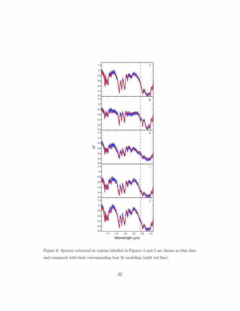
Figure 6: Spectra extracted in regions labelled in Figures 4 and 5 are shown as blue dots

and compared with their corresponding best fit modeling (solid red line).

42

CH4:N2

N2:CH4

CH4:N2

Figure 7: The fraction of a Pluto rotation period that a point at a given latitude is sunlit

versus average flux in W/m2. Northern latitudes are marked with symbols spaced at 10◦

intervals. The filled squares show the average energy flux to Pluto’s northern hemisphere

over the decade 1995-2005 while the filled circles show the same for the past ten years.

Pluto’s north pole has been sunlit since 1987 and, over the past 20 years, has received

more solar illumination than any other latitude. Differences are relatively minor around

the turn of the century, but become much more pronounced after 2005. The intense heating

correlates well with polar depletion of N2 (see the reddish circle on the Pluto inset).

43