podboy p1 cd04 - nasa
TRANSCRIPT
1
This material is declared a work of the U.S. Government and is not subject to copyright protection in the United States. Approved for public release; distribution is unlimited.
Proceedings of the ASME Turbo Expo 2012 GT2012
June 11-15, 2012, Copenhagen, Denmark
GT2012-69801
JET-SURFACE INTERACTION TEST: PHASED ARRAY NOISE SOURCE LOCALIZATION RESULTS
Gary G. Podboy
NASA Glenn Research Center Cleveland, Ohio, USA
ABSTRACT An experiment was conducted to investigate the effect that a planar surface located near a jet flow has on the noise radiated to the far-field. Two different configurations were tested: 1) a shielding configuration in which the surface was located between the jet and the far-field microphones, and 2) a reflecting configuration in which the surface was mounted on the opposite side of the jet, and thus the jet noise was free to reflect off the surface toward the microphones. Both conventional far-field microphone and phased array noise source localization measurements were obtained. This paper discusses phased array results, while a companion paper1 discusses far-field results. The phased array data show that the axial distribution of noise sources in a jet can vary greatly depending on the jet operating condition and suggests that it would first be necessary to know or be able to predict this distribution in order to be able to predict the amount of noise reduction to expect from a given shielding configuration. The data obtained on both subsonic and supersonic jets show that the noise sources associated with a given frequency of noise tend to move downstream, and therefore, would become more difficult to shield, as jet Mach number increases. The noise source localization data obtained on cold, shock-containing jets suggests that the constructive interference of sound waves that produces noise at a given frequency within a broadband shock noise hump comes primarily from a small number of shocks, rather than from all the shocks at the same time. The reflecting configuration data illustrates that the law of reflection must be satisfied in order for jet noise to reflect off of a surface to an observer, and depending on the relative locations of the jet, the surface, and the observer, only some of the jet noise sources may satisfy this requirement.
INTRODUCTION In October 2008, NASA called on industry and
academia to propose conceptual designs for advanced aircraft which could satisfy both future commercial air transportation capacity requirements and specific goals related to reductions in fuel burn, noise, and air pollution. Compared to an aircraft entering service today, NASA’s goals for a 2030-era aircraft are 1) a 71 dB cumulative reduction below current Federal Aviation Administration noise levels, 2) a greater than 75% reduction in nitrogen oxide emissions, and 3) at least a 70% reduction in fuel burn.
The four aircraft shown in Figure 1 were proposed in response to NASA’s call. These all share one characteristic: in each case the aircraft engines are located near solid surfaces. In the case of the two turboprop-driven designs, shown in parts a and b of Figure 1, the propellers are mounted upstream of the wing’s leading edge, while with the aircraft shown in part c the engine exhaust would flow under the wing. In these three cases the interaction between the flow downstream of the engine and the wing could be expected to generate increased noise relative to an engine operated in isolation. With the fourth design shown in part d, the aircraft’s fuselage would shield some of the forward-propagating fan noise from reaching the ground, resulting in decreased noise levels relative to an isolated engine.
The idea of using parts of the airframe to shield engine noise has been proposed for other aircraft as well. It is one of the noise reduction technologies included in the Hybrid Wing Body (HWB) concept aircraft developed by the Boeing Company with funding from NASA’s Environmentally Responsible Aviation Project2 and the Advanced Model for

2
This material is declared a work of the U.S. Government and is not subject to copyright protection in the United States. Approved for public release; distribution is unlimited.
Extreme Lift and Aeroacoustics (AMELIA) developed by the California Polytechnic State Institute through a three-year NASA Research Announcement grant sponsored by NASA’s Subsonic Fixed Wing Project. Both of these aircraft are shown in Figure 2. With these designs, the wing is used to shield some jet noise from reaching the ground. The amount of jet noise reduction would depend on the location of the engine nozzle relative to the trailing edge of the wing and the distribution and directivity of noise sources within the jet plume. Consequently, the location of the engine relative to the wing trailing edge is a critical aspect of design. Another consideration is that if the engine is too close to the wing’s surface or embedded in the wing such that the engine exhaust flow scrubs across the wing’s surface then low-frequency trailing edge noise will be created, mitigating some of the noise reduction potential of the shielding concept. Recently, McLaughlin et. al.3 demonstrated that noise measurements made during field tests of full-scale aircraft or aircraft engines can depend significantly on noise reflecting off the ground. They point out that when pole mounted microphones are used in such investigations that noise reaches the microphone from both a direct and a ground reflection path, and that the resulting interference leads to both positive and negative reinforcement of the sound waves. This interference depends on both the acoustic frequency and the path length difference and generates multiple humps in the measured acoustic spectra and increases the integrated mean square value of the acoustic pressure (the area under the spectral curve). They obtained data with both cold and hot Mach 1.5 jets tested in isolation and near a simulated ground plane. Using these data they developed a model that attempts to derive “free-field” noise estimates from measurements made during full-scale field experiments. They point out that the development of such a model “requires reasonably accurate information on the distribution of noise sources within the jet.”
Based on the above discussion, it is clear that in order reach NASA’s stringent noise reduction goal that the interaction between the noise and/or flow produced by an engine and any nearby solid surfaces will have to be considered. Depending on the configuration, the surface effects could lead to either increases or decreases in noise relative to an engine operated in isolation.
One goal of NASA’s Subsonic Fixed Wing Program is to develop computer programs that can accurately predict the changes in aircraft noise caused by engine installation effects. Historically, ANOPP, NASA’s most well known program for predicting the community noise generated by a given aircraft configuration, has used rather simple models of jet noise to predict the noise benefits associated with shielding. Recently, Papamosochou4 used data obtained from subscale experiments to show that these simple models do not provide accurate estimates of jet noise shielding. He argued that they were
inadequate because they approximate the jet noise as a small number of discrete point sources, when in actuality jet noise is a more complicated, distributed source. He developed a new model that describes the jet noise source as a combination of a wavepacket and a monopole. He points out, however, that in order to predict any reduction in jet noise due to shielding that a realistic jet noise model is not sufficient; it is also necessary to know the axial distribution of noise sources in the jet5. Past experiments have shown that these distributions can vary significantly depending on both the jet operating condition and the angle of the observer relative to the jet6.
Despite the importance of installation effects, there is a lack of quality experimental data on jets with surfaces nearby which could be used to develop and validate noise prediction methods. In an effort to fill this need, a series of experiments known collectively as the Jet-Surface Interaction Test (JSIT) are being conducted at the NASA John H. Glenn Research Center in Cleveland, Ohio, USA. Phase 1, completed in February 2011, was conducted in an effort to expand the database available regarding how a planar surface parallel to the jet centerline interacts with a jet to modify the noise propagating to the far field. Two different configurations were tested: 1) a shielding configuration in which the surface was located between the jet flow and the far-field microphones, and 2) a reflecting configuration in which the surface was mounted on the other side of the jet, and thus the jet noise was free to reflect off of the surface toward the microphones. The surfaces were chosen to be large relative to the size of the nozzle so that they would appear semi-infinite, i.e. extend forever upstream of the trailing edge. Three parameters were varied during the test: 1) the axial distance that the surface extended downstream of the nozzle exit, 2) the radial location of the surface relative to the jet centerline, and 3) the jet operating condition. Far-field microphone, phased array noise source localization, unsteady surface pressure, and pressure sensitive paint data were acquired during the test. Brown has presented the far-field microphone data in a companion paper.1
The purpose of the present paper is to show some
examples of the phased array noise source localization data acquired during the test. These data were acquired for two reasons. The first was to help explain the far-field microphone results. In order to understand how a surface interacts with a jet to alter the noise propagating to the far-field it is necessary know the axial distribution of noise sources within the jet. These distributions were measured for each of the jet operating conditions set during the test. They can be used to explain, for example, why a shield might be effective at blocking noise for one jet operating condition, but not for another. The second reason was to ensure that the shielding surfaces were blocking all measurable noise except for that emanating at or downstream of the surface trailing edge. The example data presented herein provide useful insights regarding how a
3
This material is declared a work of the U.S. Government and is not subject to copyright protection in the United States. Approved for public release; distribution is unlimited.
surface near a jet can alter noise levels depending on the relative locations of the jet, the surface and the observer.
NOMENCLATURE
b acoustic source strength estimated from beamforming c the speed of sound camb ambient speed of sound
cj speed of sound in jet C, CSM cross spectral matrix D nozzle exit diameter g steering vector Ma acoustic Mach number, (Vj/camb) Mj ideally-expanded Mach number, (Vj/cj) NPR nozzle total pressure ratio, (Pj total/Pamb)
OB octave band Pj nozzle plenum pressure angular frequency SPL sound pressure level Tj jet temperature
TSR nozzle static temperature ratio, (Tj static/Tamb) V velocity Vj ideally-expanded jet exit velocity w normalized steering vector x
grid point location
y
microphone location
Research Instrumentation
Test Hardware
This experiment was conducted using the Small Hot Jet Acoustic Rig (SHJAR) located at the NASA John H. Glenn Research Center (GRC) in Cleveland, Ohio, USA. SHJAR is a single-stream nozzle test rig used for fundamental jet noise research. It can accommodate air mass flow rates of up to 6 lb/sec (2.7 kg/s), nozzle exhaust temperatures ranging from ambient to 1300 F (980 K), and nozzles as large as 3 (7.62 cm) in diameter. The test rig is located within the Aeroacoustic Propulsion Laboratory (AAPL), a 19.8 m radius anechoic geodesic dome. Both the floor and the dome’s interior surface are covered with sound absorbing acoustic wedges. The facility acoustic instrumentation includes a far-field microphone array made up of 24 microphones arranged in a circular arc at 5 intervals from 50 to 165 from the jet upstream axis and located 150 (3.81 m, 75 nozzle diameters) from the nozzle exit. Brown et. al.7 provide more information regarding SHJAR and the acoustic characteristics of the AAPL facility.
The planar surfaces used during the test were mounted in the two configurations illustrated in Figure 3. The upper photo shows the shielding configuration in which the surface was located between the jet flow and the far field microphone
array; the lower photo shows the reflecting configuration, where the surface was located on the opposite side of the jet. The surfaces were 6 tall and, except near the trailing edge, were made of ½ thick aluminum plates. Plates were added and removed as necessary during the test to change the axial dimension of the surface. A separate, 6 tall x 4 wide x ¼ (1.83 m x 10.2 cm x 0.635 cm) thick aluminum strip was used to provide the surfaces with a sharp trailing edge. This strip, which was flush mounted to the downstream edge of the thicker surface, had its trailing edge cut back at a 39.2 angle such that the pointed side was on the side of the jet flow. The surfaces were mounted onto a support structure that, in turn, was mounted onto a moveable cart. The cart rode along rails that were parallel to the jet centerline and was moved manually in order to change the axial location of the surface trailing edge relative to the nozzle exit. A 1 m, linear traverse system mounted to the top of the cart was used to move the surfaces in the radial direction relative to the jet. The intent was for the surfaces used during the shielding configuration to appear semi-infinite, i.e. to block any noise coming from upstream of the surface trailing edge from reaching the far field microphones. Phased array data obtained early on in the test indicated that at times measurable noise would leak above or below the surface, or between the gap that existed between the upstream edge of the surface and the wedge wall. In order to block this noise, multiple layers of welder’s blankets were hung from a horizontal support above the top edge of the shielding surface. The blankets covered the backside of the surface and draped around the side of the wedge wall shown in Figure 3. From an acoustic standpoint, they increased the vertical height of the shield and covered the gap between the surface and the wedge wall. All of the shielding configuration phased array data presented in this report were acquired with the blankets in place. Phased array data obtained on subsonic jets after the blankets were installed confirmed that the noise coming from downstream of the surface trailing edge was always at least 10 dB greater than any noise coming around the other three sides of the surface. Similar data obtained on supersonic jets suggests that some screech tones may have either penetrated the surface/blanket barrier or, for certain shield locations, may have reflected off the backside of the shield.
Data were acquired using two SMC series nozzles that
have been tested extensively in the past at NASA Glenn, SMC000 and SMC016. SMC000 is a convergent nozzle that serves as a baseline for most SHJAR tests. SMC016 is a convergent-divergent (C-D) nozzle that was designed using the method of characteristics to provide an ideally expanded flow at Mj=1.5. Both nozzles have a 2 (5.08 cm) exit diameter.
Test Conditions
4
This material is declared a work of the U.S. Government and is not subject to copyright protection in the United States. Approved for public release; distribution is unlimited.
Table 1 provides information regarding the jet
operating conditions set during the test. The eight different jet conditions that were tested will be identified by the setpoint listed in the table. As indicated, data were acquired using the convergent SMC000 nozzle at 5 different setpoints, four of which correspond to subsonic jets. Of these four, two were cold, as was the lone supersonic case. Data were acquired using the convergent-divergent SMC016 nozzle on three cold, supersonic jets, one under-expanded, one ideally-expanded, and one over-expanded. The Phased Array System
Figure 4a shows a front view of the OptiNav Array48 phased array system used during this test. This system consists of 48 Earthworks M30 microphones flush-mounted to a 1 m x 1 m aluminum plate. The microphones are arranged in a series of log spirals in an effort to reduce sidelobes (errors in the phased array data). The microphones have ¼ (0.635 cm) diameter diaphragms and a flat frequency response over a frequency range of 5 Hz to 30 kHz. They can be used to measure sound fields with amplitudes as high as 142 dB before they begin to saturate (136 dB when flush mounted in the array plate). A photograph of the back of the microphone array is shown in Figure 4b. This photo shows the microphones mounted to the back of the array plate and a camera located at the center of the plate. There is a hole in the center of the plate through which the camera can be used to take a photo of the “field of view” of the phased array system. The phased array data reduction software superimposes the acoustic source localization data on top of the image taken with the phased array camera. The phased array data were reduced using classical beamforming in the frequency domain. The first step in the data reduction process was to compute the cross spectral matrix, C, from the array data using the periodogram method with Hanning windowing functions and 50% block overlap. The diagonal elements of the cross spectral matrix are then deleted (yielding C ), and the beamforming result, b, at a given grid point, k, is computed using the classical beamforming expression
bk w kC wk
where wk is a normalized version of the steering vector gk, and b represents the apparent strength of the acoustic source located at grid point k as estimated from the beamforming. The individual elements of gk represent the Green’s function for a monopole located at grid point k as observed by microphone i. In free space with no flow
where kx
and iy
denote the locations of grid point k and
microphone i, respectively. A beamforming result is computed for each point in a beamforming grid. The results corresponding to an entire grid are then displayed as color contour maps (known as beamform maps). Each contour map corresponds to a selected frequency band, and shows the location of the dominant noise source or sources in the band as a 2 dimensional color contour map overlaid on top of a photograph taken with the phased array camera. The color contours correspond to the location and strength of the noise sources found within an image plane (the beamform grid) parallel to the array plate at some specified distance away from the array. The dynamic range of the color contours (max value minus min value) is the same for each beamform map (i.e. processed frequency band), but the peak value can vary from map to map. The color contour maps presented later in this paper all have a 7 dB dynamic range. Phased Array and Surface Locations
All of the phased array data obtained during the
shielding tests were acquired with the array mounted on a stationary support stand located between the base of the moveable cart and the far field array (see Figure 5). With this arrangement, the shielding surface moved while the phased array and nozzle remained fixed. The center of the array was at the same height as the jet centerline, 10 (3.05 m) above the floor, and the array plate was parallel to, and 2.82 m (about 55 nozzle diameters) away from, the jet centerline. Since the nozzles have different lengths, the axial location of the phased array relative to the two nozzle exit locations was slightly different. With the SMC000 nozzle, the array was located such that a line normal to the center of the array intersected the jet centerline at the nozzle exit, while with the SMC016 nozzle the array normal intersected the jet centerline 5 (12.7 cm) upstream of the nozzle exit. The polar angle between a ray directed downstream through the jet axis and a line spanning from the array center to the center of the nozzle exit was 90 when the SMC000 nozzle was tested, and 92 with the SMC016 nozzle. The array aperture was roughly 20. Table 2 provides a list of surface locations and setpoints at which phased array data were acquired during the shielding surface tests. Data were acquired at each of the eight setpoints listed in Table 1 with the trailing edge of the surface located 2, 4, 6, 10, 15 and 20 nozzle diameters downstream of the nozzle exit. For each axial location of the surface, data were acquired at 17 different radial locations ranging from 1 to 16 diameters from the jet centerline. In this paper, the symbol “D”, which corresponds to a distance equal to the nozzle exit
5
This material is declared a work of the U.S. Government and is not subject to copyright protection in the United States. Approved for public release; distribution is unlimited.
diameter (50.8 cm), will be used to designate both how far a surface extends downstream of the nozzle exit and how far it is away from the jet centerline. For example, a surface extending 6 nozzle diameters downstream of the nozzle exit will be referred to as a 6D surface, and a surface located 4 nozzle diameters from the jet centerline will be referred to as being 4D away. A small subset of the phased array data obtained during the reflecting surface tests were acquired with the array at the same location it was at during the shielding surface tests (shown in Figure 5.) As indicated in Table 3, data were obtained with the array mounted on the stationary stand with the jet operating at two cold conditions (7 and 9010) with the surface at one axial location relative to the nozzle exit (trailing edge 6 diameters downstream of the nozzle exit) and at the same set of 17 radial locations set during the shielding tests. This array location allows back-to-back comparisons of shielding and reflecting configuration data, but also has a couple of drawbacks. One is that the noise coming from the surface is likely to show up in the phased array beamform maps at the same location as the noise coming directly from the jet, making it difficult to differentiate between them. The other is associated with the fact that the noise reflecting off or being created at the surface has to pass through the jet before reaching the phased array; this is a disadvantage since the turbulence in the jet would tend to de-correlate the sound waves coming from the surface, making it difficult to image the surface noise. All of the other phased array data obtained during the reflecting surface tests were acquired with the phased array mounted on the moveable cart, fixed with respect to the wall rather than the nozzle. As shown in the photo provided in Figure 6, the array was mounted on the cart below the jet with the array plate angled upward. This was done 1) so that the noise coming directly from the jet and the noise scattering off of the surface would show up at different locations in the beamform maps, 2) to shorten the distance between the array and the surface, and thus increase the spatial resolution of the phased array, and 3) so that the jet turbulence would not de-correlate the sound waves coming from the surface. As indicated in Table 4, reflecting surface data were acquired with the array mounted on the moveable cart at each of the same six cold setpoints tested during the shielding tests, using surfaces that extended 5, 10, 15, and 20 nozzle diameters downstream of the nozzle exit. For each axial location of the surface, data were acquired at the same set of 17 different radial locations set during the other tests. Due to time constraints, hot jet data were not acquired while the surfaces were mounted in the reflecting configuration.
RESULTS Bare Jet Results When a surface interacts with a jet, the noise heard by an observer in the far field is dependent not only on the relative locations of the surface, the jet and the observer but also on the axial distribution of noise sources in the jet. Obviously, the closer the sources are to the nozzle exit, the easier it would be to shield the noise using a surface. The directivity of jet noise is also important. Some jet noise sources, such as large turbulent eddy/shock wave interaction, are themselves directive, meaning that the noise they produce in the far field is dependent on the angle of the observer relative to the jet axis. Jet noise also has directionality due to convective amplification, the concept that states that sound levels are increased when the sources are moving toward the observer (in the downstream direction for jet noise) and reduced when they are moving away from the observer (in the upstream direction). The interaction between sound waves produced inside the jet and gradients in the jet mean flow also contributes to the directivity of jet noise. This interaction tends to bend any downstream propagating sound waves away from the jet axis. Because of the directive nature of jet noise, the noise source locations measured using a phased array will vary depending on the angle between the array and the jet axis. During this experiment, bare jet phased array data were obtained with the array at the same location that it was at during the shielding tests, i.e. broadside to the jet, roughly 55 diameters away, and at an angle approximately 90 to the jet axis. This data provides information regarding the distribution of noise sources in the jet as observed from this particular direction. It can be used to gain insights regarding why a shield might or might not be effective at blocking the noise propagating in this direction.
Figure 7 shows bare jet phased array data obtained on a cold, subsonic jet. These data were obtained using the convergent SMC000 nozzle at setpoint 3 (Ma=0.50, TSR=0.95), which corresponds to the lowest Mach number set during the test. Seven beamform maps are shown at the right in Figure 7; the upper six correspond to 1/12th octave bands centered at 1, 2, 4, 8, 16, and 32 kHz. The 1/12th octave band center frequency and corresponding Strouhal number (St) are shown in the upper left corner of each map, and the small, red square on each map corresponds to the peak noise source location. The spacing of the green grid lines superimposed on the beamform maps corresponds to a distance equal to one nozzle diameter. The plot in the upper left of the figure shows PSD spectra computed from the output of the microphone closest to the center of the array. This is conventional single-microphone spectra, not a product of the phased array beamforming. The single microphone spectra presented in this section and in the two shielding configuration sections that follow have been scaled to a distance equal to 100 nozzle diameters from the jet centerline. The single microphone
6
This material is declared a work of the U.S. Government and is not subject to copyright protection in the United States. Approved for public release; distribution is unlimited.
spectra presented later in the reflecting configuration section were not scaled in this manner since the distance between the array plate and the jet varied during that part of the test. The plot at the lower left in Figure 7 shows the distance between the peak in the beamform maps and the nozzle exit as a function of frequency, in units of nozzle diameters. This type of plot will be referred to herein as a peak location plot. Red asterisks have been superimposed on each of the two line plots at the frequencies represented by the six 1/12th octave band beamform maps at the right in the figure. The single microphone spectrum provided in Figure 7 indicates that this jet produces significant noise over a wide frequency range between St=0.17 and St=0.8 (600 and 2600 Hz), and the peak location plot shows that this noise originates between roughly 4 and 9 diameters downstream of the nozzle exit. The peak location plot also indicates that the peak source occurs about 10 nozzle diameters downstream of the nozzle exit at the lowest processed frequency (400 Hz, St=0.12), and that it gradually moves closer to the nozzle exit with increasing frequency. For frequencies above about 10 kHz (St=3.1), the peak source location is always within two nozzle diameters of the nozzle exit. At this operating condition the dominant noise sources occurring within any given frequency band do not appear to extend significantly in the axial direction. Instead, they tend to be centered about one axial location in the jet plume, although this location does vary with frequency – it gets closer to the nozzle exit with increasing frequency. The beamform map provided in the lower right hand corner of Figure 7 corresponds to the same data processed into one wide band ranging from 388 to 45,986 Hz. In that both produce a final result based on a very wide frequency range, the data processing used here is similar to that used to calculate Overall Sound Pressure Level (OASPL). Consequently, this sort of plot will be referred to herein as an OASPL beamform map. A plot such as this does not provide as much information as a set of 1/12th OB plots, but is practical for use in a technical paper since it shows the locations associated with the loudest sources in the jet in a single plot. OASPL beamform maps will be used later in the presentation of shielding configuration results. The OASPL plot shown in Figure 7 indicates that for this cold, subsonic jet the loudest sources are located between 4 and 9 diameters downstream of the nozzle exit. Figure 8 shows these Ma=0.50 data compared with results obtained with the SMC000 nozzle set to provide a higher-speed, subsonic jet (setpoint 7, Ma=0.90, TSR=0.835). As shown in the figure, the results for these two cases are similar in that they both show 1) broad, rounded spectra, and 2) the peak noise source located relatively far downstream at low frequency and moving gradually closer to the nozzle exit as frequency is increased. The main differences are 1) that the peak spectra levels are about 20 dB higher, and 2) the peak source location starts out further downstream (11.5 vs. 10
diameters) at low frequency in the higher speed jet. A comparison of the OASPL beamform maps indicates that the loudest noise occurring at a given frequency is generated about 2 diameters further downstream in the higher speed jet. The peak location plot provided in the upper right corner of the figure indicates, however, that plotting the peak source location vs. St (rather than frequency) tends to collapse the data from the two jets to a single line, especially for St>0.5. The results just discussed (Figures 7 and 8) correspond to cold, subsonic jets. Figure 9 provides information regarding the changes that occur when heat is added to a cold, subsonic jet in such a way that acoustic Mach number (jet velocity) is maintained. The beamform maps presented in Figure 9 correspond to setpoints 27 (NPR=1.36, TSR=1.76, Ma=0.90) and 46 (NPR=1.24, TSR=2.70,
Ma=0.90). The spectra and peak location plots presented at the top of the figure show results for both of these hot jets, as well as for a cold jet at the same acoustic Mach number (setpoint 7, shown previously in Figure 8). The spectra indicate that adding heat while maintaining the same jet velocity tends to reduce the level of high frequency noise propagating in the direction of the array (90 to the jet axis) by as much as 5 dB. Meanwhile, the peak location plots show that the noise sources corresponding to any given frequency tend to move upstream if heat is added while acoustic Mach number is held constant. For example, the source location of the lowest processed frequency band, 400 Hz (St=0.07), moves steadily upstream from 14 to 8 diameters downstream of the nozzle exit as TSR is increased from 0.835 to 2.70. In this case acoustic Mach number was maintained, but jet Mach number decreased when heat was added, and the peak source locations corresponding to any given frequency moved upstream. Results from a previous test8 indicate that if heat is added such that jet Mach number is maintained then the source locations corresponding to any given frequency do not change. This indicates that jet Mach number (or NPR) dictates where the turbulent mixing noise generated at any given frequency comes from in the jet – the sources move downstream as jet Mach number increases. All of the subsonic jet results presented above show 1) broad haystack-like spectra, and 2) the peak noise source location moving steadily upstream as frequency is increased. All of these results are similar because in subsonic jets there is only one source of noise, the turbulent mixing that occurs between the jet and the ambient air. Figure 10 shows results from data acquired with the convergent-divergent SMC016 nozzle at 3 supersonic setpoints (11606 over-expanded, 11610 ideally-expanded, and 11610 under-expanded). The ten points labeled along the spectra and peak location line plots correspond to the ten 1/12th octave band beamform maps shown for each setpoint. At low frequency (St<0.3), both the spectra and peak location plots generated from the supersonic jets resemble the subsonic
7
This material is declared a work of the U.S. Government and is not subject to copyright protection in the United States. Approved for public release; distribution is unlimited.
results discussed earlier, suggesting that turbulent mixing noise is dominant in this frequency range. A fundamental screech tone occurs at St=0.41 (3000 Hz, pt 2, blue line plots) in the over-expanded jet data and appears in the corresponding beamform map (#2, left column) predominantly as a reflection off of the upstream nozzle hardware. A harmonic of the fundamental screech tone occurs at St=0.82 (6000 Hz, pt 5, blue line plots) and comes directly from a location in the jet plume about 5 diameters downstream of the nozzle exit. Broadband shock noise (BBSN) shows up clearly in the spectra presented in Figure 10 for the two off-design operating conditions as the elevated region at high frequency (to the right of pt 3 for the over-expanded case and to the right of pt 2 for the under-expanded). A dominant BBSN hump is clearly visible in the spectrum for the under-expanded jet between St=0.35 and St=0.87 (3000 and 7500 Hz, magenta spectrum, between points 2 and 6). The 1/12th octave band beamform maps provided for the under-expanded jet (right column) indicate that the location of the peak noise source moves downstream as frequency increases through this BBSN hump (beamform maps 3 through 6). Then, at a frequency beyond the hump (to the right of point 6 on the magenta spectrum) the peak noise source location jumps back upstream, before this pattern (downstream movement followed by a jump back upstream) repeats once again (points 7 thru 9). This upstream-downstream-upstream-downstream movement of the peak noise source location shows up in the peak location plots as the repeated shark-fin-like pattern. Note that it shows up not only in results obtained for the off-design cases (magenta and blue), but also at the design condition (green). This sort of pattern has also been seen in the peak location plots generated from data obtained on other supersonic jets8. The spectrum provided in Figure 10 for the under-expanded case (magenta) shows one dominant hump rising above the higher frequency broadband shock noise, to the right of the hump. The BBSN theory put forth by Tam9 suggests that the elevated region of high frequency noise is actually made up of a series of humps centered about different frequencies. These humps are illustrated in Figure 11 (taken from Miller10). Sometimes multiple humps are visible in the acoustic spectra obtained from shock-containing jets. Normally, however, the lowest frequency hump is much easier to identify than the others. These humps are thought to be created by turbulent eddies which are large enough to span more than one shock cell. The interaction of these large eddies with the shocks generates highly correlated noise radiating from multiple shocks simultaneously. According to Harper-Bourne and Fisher11, at the peak frequency in each hump “radiation from all sources interferes constructively,” while on either side of the peak “this constructive interference is less complete and hence lower levels of noise are anticipated.” The lowest frequency hump is created by the interference of sound waves coming from adjacent shocks (1 shock spacing part), the second hump
is created by the interference of waves coming from every-other shock (2 shock spacings apart), etc. Using Tam’s model, Miller12 calculated the peak frequencies of the humps corresponding to the two off-design operating conditions tested with the C-D SMC016 nozzle. Figure 12 shows the peak frequencies corresponding to the two lowest frequency humps (asterisks) overlaid on top of the spectra and peak location plots for the over-expanded and under-expanded jet data shown previously in Figure 10. As shown in the peak location plots, the predicted hump peak frequencies occur very close to the centers of the first two shark-fin patterns that are shown for each operating condition. This good correlation suggests that the mechanism that creates the spectral humps in Tam’s model (large eddy/shock wave interaction) is also responsible for the downstream-upstream-downstream-upstream movement of the peak noise source location that occurs as frequency increases. It also implies that the peak location plots show where the large eddy/shock wave interaction that produces the humps occurs at in the jet. In the over-expanded case, the first hump is created by shocks located between 4 and 8 diameters downstream of the nozzle exit; the second hump by shocks between 5 and 7 diameters downstream. For the under-expanded jet the first hump is created by shocks between 8 and 17 diameters downstream, and the second hump by shocks between 12 and 15 diameters downstream. In both jets, some of the same shocks that produce the first hump also produce the second. The individual beamform maps shown in Figure 10 corresponding to the first hump (the first downstream movement of the peak source, maps 4 thru 7 in the left column, and maps 3 thru 5 in the right column) indicate that any given frequency in a hump is generated from a relatively small axial region in the jet. This suggests that the constructive interference of sound waves that produces the noise at a given frequency and observer location comes primarily from a small number of shocks, rather than from all the shocks at the same time. It is interesting that the repeated shark-fin pattern also appears in the peak location plot provided in Figure 10 for the design condition (setpoint 11610, green line) even though any shocks occurring in the jet at this condition are likely to be much weaker than at the two off-design conditions. The beamform map given for the 1/12th OB centered at 30 kHz (St=3.7, map #10, center column) shows that shocks were present in the jet at this operating condition (it was not quite ideally-expanded). The presence of the shark-fin pattern suggests that the large eddy/shock wave interaction mechanism also occurred at this condition, but the spectrum shown in Figure 10 (green) indicates that the noise produced by this interaction was not loud enough to produce a distinct BBSN hump. At least for this case, it appears that the downstream movement of the peak source location is a more sensitive indicator of the presence of large eddy/shock wave interaction than the spectrum itself.
8
This material is declared a work of the U.S. Government and is not subject to copyright protection in the United States. Approved for public release; distribution is unlimited.
The subsonic jet data presented earlier showed that the peak source location associated with any given frequency of noise tends to move downstream as NPR (or jet Mach number) increases. A comparison of the three peak location plots presented in Figure 10 shows this to be true in supersonic jets as well. This is indicated not only for the low frequency region controlled by turbulent mixing but also for the high frequency region where large eddy/shock wave interaction produces the shark-fin pattern observed in the peak location plots. This means that the shocks which interact with the large turbulent eddies to produce the BBSN humps are, on average, located further away from the nozzle the higher the nozzle pressure ratio. The 1/12th OB beamform maps presented in Figure 10 for the over-expanded condition (left column) are noticeably different than those provided for the two higher jet Mach numbers (center and right columns). None of the color contours shown in the beamform maps for the over-expanded condition extend very far downstream of the peak noise source location (the location of the small red square), whereas some of the contours provided for the two higher speed jets do. This has important implications regarding jet noise shielding. A shield that extends a couple of nozzle diameters further downstream than the peak noise source location in the over-expanded jet would block almost all of the noise associated with that frequency band, while a surface placed in a similar manner in the higher speed jets could still allow much of the noise to propagate in the direction of the phased array. A surface extending 10 diameters downstream of the nozzle exit, for example, placed next to the ideally-expanded jet would cover the peak source location shown in beamform map #8 (center column), but a significant portion (about 5 diameters) of the noise-producing region of the jet would remain uncovered. This means that in order to effectively shield the noise produced by a jet it may not be enough to know the location of the peak noise source as a function of frequency (information provided by the peak location plots). It might also be necessary to know how far the noise producing regions extend downstream of the peak source location in each frequency band (information provided by the 1/12th OB plots).
Figure 13 shows all the peak source location data presented previously on the same plot. Unlike the preceding plots, however, the peak source location data presented here have been nondimensionalized by potential core length. The potential core length corresponding to each setpoint was estimated from the Witze correlation parameter13 following the
method outlined by Bridges et. al.14 As shown in the figure, the nondimensional peak source location vs. nondimensional frequency curves for the four subsonic test cases tend to collapse to one distribution. The low-frequency portion of the curve provided for the ideally-expanded supersonic case (setpoint 11610, green) also collapses, but the low-frequency
segment of the curve provided for the under-expanded case (setpoint 11617, magenta) is slightly higher, and that of the over-expanded case (setpoint 11606, blue) is much lower than this distribution. This suggests that this method of nondimensionalizing data collapses the low frequency region of supersonic jet peak source location data only when strong shocks are not present in the flow. The presence of the shocks appears to bias the low frequency source location data of under- and over-expanded supersonic jets toward the location of the shocks (i.e. closer to the nozzle for over-expanded jets and further from the nozzle for under-expanded). At higher frequencies, where the shark-fin pattern occurs, none of supersonic source location data collapse; this shock noise is generated further downstream as jet Mach number increases. Shielding Configuration, Subsonic Jet Results A surface placed between a jet plume and an observer can act as a shield, but it can also act as a noise source. If the surface is located so close to the jet that the flow impinges on the surface then additional noise will be generated 1) by the turbulent flow “scrubbing” along the surface and 2) at the trailing edge where hydrodynamic pressure fluctuations are scattered into acoustic waves. Shielding configuration data will be presented below for surfaces located 1, 2, and 3 diameters from the jet centerline. The schematic presented in Figure 14 shows the axial location at which each of these surfaces could be expected to first intersect a jet that is assumed to expand at a 7 angle. It shows that surfaces located 1, 2, and 3 diameters from and parallel to the jet centerline could be expected to intersect the jet roughly 4, 11.5, and 20 nozzle diameters downstream of the nozzle exit, respectively. This means, for example, that a surface located 1D away from the centerline and extending 2D downstream of the nozzle exit would not be expected to generate scrubbing noise, but a surface at the same radial location and extending 6D downstream would. The bare jet data presented in the preceding section indicates that subsonic jets are relatively simple in comparison to supersonic jets. In both cold and hot subsonic jets there is only one source of noise, turbulent mixing, and the peak noise source location occurs relatively far downstream at low frequency and moves gradually upstream as frequency increases. Therefore, it would be more difficult to shield low frequency vs. high frequency noise in a subsonic jet. Also, the peak noise source location corresponding to any given acoustic frequency moves upstream toward the nozzle as jet Mach number decreases. Consequently, it would become increasingly more difficult to shield the jet noise coming from a subsonic jet as the jet Mach number increases. Of the five subsonic operating conditions set during the test, setpoint 7 (Ma=0.90, TSR=0.835) corresponds to the highest jet Mach number, and therefore, the most difficult to shield. Figure 15 shows shielding configuration phased array
9
This material is declared a work of the U.S. Government and is not subject to copyright protection in the United States. Approved for public release; distribution is unlimited.
data obtained at this operating condition with surfaces located 3 nozzle diameters (3D) away from the jet centerline. OASPL beamform maps (right) and single microphone spectra (upper left) are provided for the bare jet as well as for surfaces that extended 2, 4, 6, 10, 15 and 20 diameters downstream of the nozzle exit. The center, left plot shows the difference between the single microphone spectrum levels measured with the bare jet and with each surface. As such, it shows the noise attenuation provided by each surface, and will be referred to herein as an attenuation plot (a positive value indicates that the surface reduced noise). The peak location plot shown in the lower left corner shows only the bare jet (no surface) distribution. In order to better visualize the noise source locations relative to the nozzle hardware, the phased array contour maps are superimposed onto a photo that was taken when the shielding surface was not in place. The vertical red line shown on all but the top map (the bare jet map) designates the location of the trailing edge of the shielding surface used in each case. Note that this line does not always match up with the grid line corresponding to a given axial location in the jet. The vertical red line shown for the 6D wall, for example, is located about 6.3 nozzle diameters downstream of the nozzle exit, while that shown for the 20D wall is about 20.7 diameters downstream. These differences are due to parallax. Since the array was always upstream of the surface trailing edge, from the viewpoint of the array camera the surfaces blocked more of the jet than would be suggested by the wall trailing edge locations (2D, 4D, etc.). These differences increased as 1) the trailing edge of the surface shifted downstream and 2) the surface moved outward away from the jet centerline and toward the array. The bare jet beamform map presented in Figure 15 (top) indicates that at this condition the loudest jet noise is generated between approximately 4 and 9 diameters downstream of the nozzle exit. Based on this, it is not surprising that the data presented for surfaces that extend only 2 or 4 nozzle diameters (2D or 4D) downstream of the nozzle exit show only small amounts of noise attenuation (up to 2 dB at high frequency), while a surface that extends 6D downstream blocks roughly half of the noise-producing region of the jet and reduces high frequency noise by about 5 dB. A surface that extends 10D downstream blocks the noise coming directly from the peak noise source location (designated by the red square in the bare jet beamform map) and reduces noise by as much as 10 dB at high frequency, while 15D and 20D surfaces provide as much as 17 and 20 dB of high-frequency noise attenuation, respectively. The data presented in Figure 15 indicate that none of the surfaces were effective at reducing low frequency noise, below St=0.17 (1 kHz). The bare jet peak location plot suggests that the two longest surfaces, 15D and 20D, should block the regions in the jet where this low frequency noise is generated, but rather than a reduction, the corresponding attenuation plots
show an increase in noise relative to the bare jet. In fact, these data indicate that having the 10D surface located 3 jet diameters from the jet centerline also results in the production of low frequency noise. The schematic shown in Figure 14 suggests that a surface located 3 jet diameters from the jet centerline would not be expected to intersect the jet plume unless it extended 20 or more jet diameters downstream of the nozzle exit. In order to impinge upon a surface that extended only 10D downstream of the nozzle exit the jet would have to expand at an angle of about 15 rather than the 7 assumed in the schematic. Huang et. al.15 conducted a similar shielding experiment using a surface next to a jet. Using pitot probe surveys they verified that excess low frequency noise can be produced even when the jet does not come in contact with the surface. Consequently, it may be that the additional noise associated with the 10D and 15D surfaces shown in Figure 15 is not caused by the flow scrubbing the surface. Instead, it may be due to the conversion of hydrodynamic pressure fluctuations into acoustic waves along the surface or at the trailing edge. Regardless of the source, these data indicate that it is not correct to assume that a surface located just outside of a 7 jet expansion cone would not generate any additional low frequency noise. The data shown in Figure 15 correspond to surfaces located 3D from the jet centerline. Figures 16 and 17 show the same type of plots for surfaces located closer to the jet, 2D and 1D from the jet centerline, respectively. A comparison of the spectra provided in these 3 figures indicates that when a surface is moved inward toward the jet centerline both the level and upper frequency of the noise generated by the jet-surface interaction increases. This is shown, for example, in the spectra provided for the 6D surface (cyan). When this surface is 3D from the jet centerline (Figure 15), the spectra is slightly (< 2 dB) above that of the bare jet (dark blue) out to about St=0.25 (1500 Hz). When it is 2D from the jet centerline (Figure 16) the noise level is as much as 3 to 4 dB above that of the bare jet and noise is produced out to about St=0.35 (2000 Hz). When this surface is moved to 1D from the centerline (Figure 17) the noise level exceeds the bare jet case by as much as 10 dB and extends out to St=0.6 (3500 Hz). The increase in level is not surprising considering that the flow scrubs across more and more of the surface as it is moved inward toward the jet centerline. The increase in frequency might be associated with the fact that as the surface is moved inward the jet/surface impingement point would move upstream. As it does the average size of the turbulent eddies interacting with the surface would tend to decrease, and the frequency of the noise resulting from this interaction would tend to increase. Shielding Configuration, Supersonic Jet Results

10
This material is declared a work of the U.S. Government and is not subject to copyright protection in the United States. Approved for public release; distribution is unlimited.
The bare jet data presented earlier suggests that it could be much more difficult to shield noise propagating in the direction of the array (roughly 90 to the jet axis) coming from a supersonic, as opposed to a subsonic, jet. In subsonic jets the peak noise source location moves gradually toward the nozzle exit as frequency increases. In contrast, in cold, shock- containing jets the source location data tend to show a rather complicated behavior in which the peak source location moves downstream as frequency increases through a BBSN hump. Consequently, it would be more difficult to shield the higher frequency noise to the right of the peak in a BBSN hump than it would be to shield the lower frequency noise to the left. The data presented earlier also show that the peak noise source location associated with any given frequency of noise tends to move downstream as NPR increases. Consequently, it would become increasingly more difficult to shield the jet noise coming from a supersonic jet as the jet Mach number increases. As discussed earlier, this was also the case for subsonic jets. Figure 18 shows shielding configuration data obtained on the SMC016 nozzle at the lowest of the 3 jet Mach numbers set using this nozzle (over-expanded setpoint 11606, Ma=1.13, TSR=0.76). The bare jet peak location plot provided in this figure (lower left) indicates that the source location associated with the fundamental screech tone (at St=0.41, 3000 Hz) was upstream of the nozzle exit. The 1/12th OB beamform map corresponding to this frequency provided in Figure 10 (#2, left column), shows that this screech tone reflected off of the upstream nozzle hardware. Except for this one tone, the peak location plot shown in Figure 18 indicates that all of the other peak noise sources associated with St > 0.13 (1 kHz) are confined to a relatively small axial region in the jet between 4 and 8 diameters downstream of the nozzle exit. By far the loudest source is the harmonic of the screech tone (St=0.82, 6000 Hz) generated 5D downstream of the nozzle exit. Since it is more than 7 dB (the dynamic range of the color maps) higher than any other source, it is the only source visible in the bare jet beamform map. Based on the bare jet data, it is not surprising that the shielding configuration data presented in Figure 18 indicates that a surface extending only 4D downstream of the nozzle exit provides very little noise attenuation (red line). A surface extending only two diameters further downstream (to 6D), on the other hand, would 1) cover about half of the noise-producing region in the jet, 2) cover the locations in the jet producing the lower frequency noise to the left of the peak of the lowest-frequency BBSN hump but not the higher frequency noise to the right, and 3) completely cover the location where the dominant screech tone is generated. The data presented for the 6D surface indicates that it provided 20 dB of noise attenuation at the frequency of the dominant screech tone (St=0.82, 6000 Hz) but only as little as 3 dB of attenuation at frequencies corresponding to the high frequency side of the lowest-frequency BBSN hump. The peak location plot indicates that the noise corresponding to the high-frequency side of this hump is generated downstream of the
trailing edge of the 6D surface, between 6 and 7.5 diameters downstream of the nozzle exit. Consequently, it is not surprising that the 6D surface would not provide much attenuation in this frequency range. A surface that extends greater than 8 diameters downstream of the nozzle exit would, however, cover most of the regions in the jet responsible for producing the elevated region of BBSN (> St=0.55, or 4000 Hz). The data presented for the 10D surface indicates that it was very effective at reducing this noise (by about 20 dB). In fact, this 10D surface was so effective at blocking the noise that relatively little additional attenuation was achieved by employing the two longer (15D and 20D) surfaces. Similar data obtained using the C-D nozzle at the ideally-expanded operating condition (setpoint 11610, Ma=1.31, TSR=0.72) are shown in Figure 19. The bare jet beamform map indicates that the loudest noise is produced relatively far downstream in the jet, between 7 and 14 diameters downstream of the nozzle exit. This suggests that a surface extending at least 15 diameters downstream of the nozzle exit would be needed to block the loudest part of the jet. Based on this it makes sense that the 10D surface provides < 5 dB of attenuation at St<1.4 (11 kHz) and a maximum of 10 dB of attenuation at the highest plotted frequency. Unlike the over-expanded case in which the 10D surface completely blocked the loudest noise-producing region in the jet and the 15D and 20D surfaces provided little additional benefit, in this case the 15D and 20D surfaces provide about 10 and 15 dB, respectively, of additional attenuation relative to the 10D surface at St>0.6 (6 kHz). Figure 20 shows the same type of data obtained using the C-D nozzle at the high Mach number test case (under-expanded setpoint 11617, Ma=1.41, TSR=0.76). At almost all frequencies the peak noise source locations plotted in this figure are downstream of those provided in Figure 19 for the ideally-expanded case. In this higher speed jet a surface extending 10D downstream of the nozzle exit would only block some of the peak noise source locations associated with the noise occurring 1) to the left of the peak of the dominant BBSN hump and 2) at St>2.5 (22 kHz). Based on this it is not surprising that the 10D surface provides < 5 dB of attenuation over the entire frequency range. The 1/12th OB beamform maps presented above in Figure 10 corresponding to frequencies to the right of the peak of the dominant BBSN hump (beamform map #5 and #6, right column) indicate that the large eddy/shock wave interaction responsible for producing this noise occurs more than 10 diameters downstream of the nozzle exit. The spectra shown in Figure 20 for the bare jet and the 10D surface overlap within this frequency range, indicating 1) that the 10D surface provides no attenuation of this noise, 2) that all of the associated noise sources must be located more than 10 diameters downstream of the nozzle exit, and therefore, 3) that the 1/12th OB beamform map is correct in showing these sources more than 10 diameters downstream. The peak
11
This material is declared a work of the U.S. Government and is not subject to copyright protection in the United States. Approved for public release; distribution is unlimited.
location plot also indicates that a surface that extends 15 diameters downstream of the nozzle would be much more effective than a 10D surface at blocking the noise produced by this jet. A 15D surface would block the peak noise source locations associated with 1) the turbulent mixing noise occurring in the range 0.15<St<0.38 (1500<f<3300 Hz), 2) the lower frequency noise to the left of the peak of the dominant BBSN hump, and 3) most and the high frequency noise to the right of the dominant BBSN hump. The spectra provided in Figure 20 indicate that the 15D surface was effective at blocking noise within these frequency ranges, especially the noise to the left of the peak in the BBSN hump (which was reduced by as much as 15 dB). These data indicate, however, that even the 15D surface would not extend far enough downstream to block all of the measurable noise coming directly from the jet. In particular, it would not block 1) the BBSN to the right of the peak in the dominant BBSN hump and 2) some of the higher frequency BBSN generated at frequencies to the right of the hump. The spectra provided in Figure 20 indicate that the 20D surface was effective at blocking noise that was not blocked by the 15D surface. For St>0.6 (above the peak in the BBSN hump) the attenuation provided by the 20D surface was roughly double that provided by the 15D surface. Comment on Source Localization Data Accuracy Numerous examples have been presented above which show that when the source locations measured in a bare jet using the phased array were subsequently blocked with a surface that the noise measured by the microphone closest to the center of the array was reduced. In other words, there is a consistency between the single microphone spectra and the phased array noise source localization measurements. This consistency tends to validate the accuracy of the phased array noise source localization data. This is important because the data processing used here assumes that the noise sources in the jet are stationary, incoherent monopoles. In the past some people have dismissed jet phased array data processed in this manner because they feel that this source model is too simplistic. They argue that a source model must take into account the fact that jet noise is produced by extended, moving, coherent structures. The data presented above indicates that using a simple, incoherent monopole source model provides accurate source localization data, at least as in cases such as this, where the phased array is 90 to the jet axis. Reflecting Configuration Results This section will discuss results obtained with surfaces mounted on the opposite side of the jet during the reflecting configuration part of the test. These data were acquired with the phased array mounted below the jet on the moveable cart with the array plate angled upward (see Figure 6). It is important to realize that in order for noise reflecting off of a surface to be
sensed by a microphone in the array that the law of reflection must be satisfied. Depending on the relative locations of the jet, the surface, and the microphone only some of the jet noise sources may satisfy this requirement. This is illustrated in Figure 21. The schematic provided in this figure shows a top view of a reflecting surface configuration test in which the surface (depicted by the red line) extends 5D downstream of the nozzle exit and is located 4D from the jet centerline. The black, vertical line represents a line normal to the array plate drawn from the center of the array. The dark blue lines labeled 1 and 2 illustrate the law of reflection for noise reflecting off of the surface trailing edge to the microphone located at the center of the array. With this configuration any jet noise sources downstream of line 2 cannot satisfy the law of reflection, and therefore, cannot reflect from the surface in such a way that they can be sensed by the microphone at the center of the array, while all sources upstream of this line can. This is important because the quality of the beamforming images of the reflected noise increases as the number of microphones that can sense it increases. Consequently, for the configuration depicted here it is unlikely that the phased array would be able to produce images of the noise reflecting off of the surface from locations in the jet downstream of the surface trailing edge. As mentioned above, reflecting configuration phased array data were obtained with surfaces that extended 5, 10, 15 and 20 diameters downstream of the nozzle exit. For the 5D surface, the phased array data were actually acquired twice; once with the reflecting surface in place, and once again on the bare jet after the surface was taken down. Having both sets of data allows the bare jet cross-spectral matrix (CSM) to be subtracted from that of the jet/surface combination. Assuming that the jet noise is the same in both cases (i.e. that the jet noise is not modified by the presence of the surface), subtracting the bare jet CSM from that of the jet/surface combination yields a CSM corresponding to the noise coming directly from the surface, and processing the resulting CSM provides better images of this noise. This is a way of “turning off” the noise coming directly from the bare jet to the array in order to better image the noise that is either generated at or reflected off of the surface. Figure 22 shows data obtained using the SMC000 nozzle at setpoint 7 (Ma=0.90, TSR=0.835) that was processed in this manner. The configuration was the same as that depicted in Figure 21; the surface extended 5D downstream of the nozzle exit and was located 4D from the jet centerline. The beamform maps shown in this figure were computed from CSMs corresponding to 1) the bare jet (left column), 2) the jet/surface combination (center column), and 3) the jet/surface combination minus the bare jet (right column). As such, the right column of beamform maps show noise coming from the surface in the absence of noise coming directly from the jet. Beamform maps are shown for five different 1/3rd octave bands. The line plots in the upper left show the beamform map
12
This material is declared a work of the U.S. Government and is not subject to copyright protection in the United States. Approved for public release; distribution is unlimited.
peak contour levels as a function of nondimensional frequency for the three datasets, and the line plots to the right show single microphone spectra for both the bare jet and the jet/surface combination. The beamform map peak spectra (left line plots) provided in Figure 22 show two distinctly different frequency regions. For St<0.6 (3.5 kHz), the jet noise source is stronger than the source associated with the surface alone, whereas above this frequency they are almost equal. The beamform maps presented for the jet/surface combination (center column) can be used to explain this difference. They show that the source of low frequency jet noise is located downstream of the surface trailing edge. Consequently, this low frequency noise does not satisfy the law of reflection and cannot reflect off of the surface towards the phased array. As frequency increases, however, the peak noise source location moves upstream, and near St=0.6 (3.5 kHz), it moves upstream of the trailing edge of the surface. Once it does 1) the law of reflection is satisfied, 2) the corresponding noise reflects off of the surface efficiently toward the array, 3) the amplitude of the reflected noise becomes essentially equal to that of the noise coming directly from the jet, and 4) the two sources combine together to produce the increased noise levels shown in the single microphone spectra (as evidenced by the green line being higher than the blue in the upper right plot). Figure 23 shows results obtained using this 5D surface at the same jet operating condition but with surface located closer to the jet, only one nozzle diameter from the jet centerline. The data provided above in Figure 22 showed that when this surface was located 4D from the jet centerline that the amplitude of the low frequency noise coming from the surface was lower than that coming directly from the jet. In contrast, the beamform map peak spectra provided in Figure 23 indicate that when the surface is only 1D from the centerline the surface is the dominant source of low frequency noise (magenta higher than blue). The beamform maps provided for the jet/surface combination (center column) show this low frequency noise coming from the surface trailing edge, rather than further downstream in the jet like it did when the surface was further away. This appears to be scrubbing and/or trailing edge noise created by the jet flow impinging on the surface. For St>0.6 the beamform map peak spectra resembles that shown previously (Figure 22) for the case when the surface was further from the jet centerline. This suggests that the mechanism responsible for the high frequency noise coming from the surface is the same in both cases, and therefore, that it is simply a reflection of the jet noise off of the surface and not due to flow scrubbing. The beamform maps provided for the jet/surface combination (center column) in Figure 23 show the low frequency scrubbing noise coming from the surface trailing edge. This is to be expected since as shown in the schematic at
the top of Figure 23 this is the only part of the 5D surface that would be impacted by the flow. Figure 24 shows data obtained with a surface that extended much further downstream, 20 diameters downstream of the nozzle exit. The beamform maps at the right correspond to jet/surface combination data obtained with this 20D surface located 1 diameter from the jet centerline. The line plots at the left show single microphone spectra for this case (surface 1D from the centerline, blue) and also for this surface located outside the jet plume, 6 diameters from the jet centerline (green). Once again, the increase in low frequency noise generated with the surface in the flow vs. out of the flow (blue vs. green in the spectra) is due to the flow coming in contact with the surface. The corresponding beamform maps show that the vast majority of this additional noise is generated at the surface trailing edge even though much of the surface upstream of the trailing edge is also impacted by the jet flow (see the schematic presented in the figure). Near 1 kHz the peak noise source location jumps from the trailing edge to an upstream location, and then gradually moves upstream toward the nozzle exit as frequency increases. This gradual upstream movement of the peak source location is similar to that which occurs in a bare subsonic jet. For frequencies above 1 kHz the in-flow vs. out-of-flow spectra almost overlap, indicating that scrubbing noise does not does contribute significantly to the noise produced by the in-flow surface at higher frequencies. Instead, this higher frequency noise seems to be just a combination of the jet noise 1) coming directly from the jet, and 2) reflecting off of the surface. When the surface is in the flow there appear to be two different competing sources: 1) the trailing edge noise, and 2) the jet noise (which reaches the array both directly and via reflection off the surface). At low frequency, the trailing edge noise dominates, while at high frequency the jet noise dominates. SUMMARY
1) Both bare jet and shielding configuration noise source
localization data were acquired with the Array48 phased array system using two nozzles, one convergent and one convergent-divergent, over a wide range of operating conditions. These data were obtained with the array at an angle approximately 90 to the jet axis, and provide information regarding the distribution of noise sources in the jet as observed from this particular direction.
2) Bare jet phased array data acquired on subsonic jets show that the sources of low frequency noise are located relatively far downstream and that the sources move gradually upstream toward the nozzle exit as frequency increases. These data indicate that it would be more difficult (i.e. require a longer surface) to shield low frequency as opposed to high frequency noise in a subsonic jet. These data also show that the source location corresponding to a given frequency of noise produced in a subsonic jet is controlled solely by jet Mach number (changing the jet temperature while holding jet Mach
13
This material is declared a work of the U.S. Government and is not subject to copyright protection in the United States. Approved for public release; distribution is unlimited.
number fixed has no effect). These data indicate that it would become increasingly more difficult to shield the noise coming from a subsonic jet as the jet Mach number increases.
3) The source location data obtained on cold, shock-containing jets tend to show a rather complicated behavior in which the peak source location moves upstream, then downstream, then upstream again as frequency increases. The downstream movement correlates well with the location of the spectral humps predicted by Tam’s BBSN model. This indicates that the mechanism thought to be responsible for creating the humps, large turbulent eddy/shock wave interaction, is also responsible for this downstream movement. Since the source location moves downstream as frequency increases through a hump it would be more difficult to shield the higher frequency noise to the right of the peak in a BBSN hump than the lower frequency noise to the left.
4) The phased array data obtained on cold, shock-containing jets also show that the eddy/shock wave interaction which produces the spectral humps occurs further and further downstream as jet Mach number increases. Accordingly, the shielding configuration data showed that it was much more difficult to shield the noise produced by an under-expanded, as opposed to an over-expanded, jet.
5) The phased array data obtained on cold, shock-containing jets also show that any given frequency in a BBSN hump is generated from a relatively small axial region in the jet. This suggests that the constructive interference of sound waves that produces the noise at a given frequency and observer location comes primarily from a small number of shocks, rather than from all the shocks at the same time.
6) The single microphone spectra measured using a C-D nozzle operating very close to its design point (Mach 1.50) resembled that of a subsonic jet (broad and round, with no screech tones or distinctive BBSN humps), but the peak noise source location plot did not. Instead of moving gradually upstream as frequency increased (like in a subsonic jet), there were some frequency ranges over which the peak noise source location moved downstream (like in the over-expanded and under-expanded jets). This suggests that although noise levels tend to decrease when a cold, over-expanded supersonic jet is brought closer to its design point, the noise source locations may become more difficult to shield because they move downstream. In regards to shielding, jet Mach number appears to be a more important variable than how far-off design the jet is operating. Like in subsonic jets, the noise produced by supersonic jets becomes more difficult to shield as jet Mach number increases.
7) Numerous examples are presented which show that when the source locations measured in a bare jet using the phased array were subsequently blocked with a surface that the noise measured by the microphone closest to the center of the array was reduced. This consistency tends to
validate the accuracy of the phased array noise source localization data and the legitimacy of the stationary, incoherent monopole source model used to process it.
8) Reflecting configuration noise source localization data are presented for a convergent nozzle operating at a high subsonic Mach number. These data illustrate that the law of reflection must be satisfied in order for jet noise to reflect off of a surface to an observer. Depending on the relative locations of the jet, the surface, and the observer only some of the jet noise sources may satisfy this requirement.
9) The low frequency noise created when the jet flow impinges on the surface was found to come primarily from the trailing edge regardless of the axial extent of the surface impacted by the flow.
ACKNOWLEDGEMENTS The NASA Fundamental Aeronautics Program, Subsonic Fixed Wing Project, supported this work. Special thanks to Steven A. E. Miller of NASA Langley for his insights regarding the origins of broadband shock noise.
REFERENCES 1) Brown, C.A., “Jet-Surface Interaction Test: Far-Field Noise
Results,” ASME paper GT2012-69639, June 2012. 2) Collier, F., Thomas, R., Burley, C., Nickol, C., Lee, C-M,
Tong, M., “Environmentally Responsible Aviation - Real Solutions for Environmental Challenges Facing Aviation,” presented at the 27th International Congress of the Aeronautical Sciences, Sept. 2010.
3) McLaughlin, D.K., Kuo, C.W., and Papamoschou, D., “Experiments on the Effect of Ground Reflections on Supersonic Jet Noise,” AIAA paper 2008-22, January 2008.
4) Papamoschou, D. “Prediction of Jet Noise Shielding,” AIAA paper 2010-653, January 2010.
5) Kawai, R.T., “Acoustic Prediction Methodology and Test Validation for an Efficient Low-Noise Hybrid Wing Body Subsonic Transport,” Final report for NASA Contract Number NNL07AA54C, February 2011.
6) Dougherty, R.P., Podboy, G.G. “Improved Phased Array Imaging of a Model Jet,” AIAA paper 2009-3186, May 2008.
7) Brown, C.A. and Bridges, J.E., “Small Hot Jet Acoustic Rig Validation,” NASA TM 2006-214234, April 2006.
8) Podboy, G.G., Bridges, J.E., Henderson, B.S., “Phased Array Noise Source Localization Measurements of an F404 Nozzle Plume at Both Full and Model Scale,” ASME paper GT2010-22601, June 2010.
9) Tam, C.K.W., “Stochastic Model Theory of Broadband Shock Associated Noise from Supersonic Jets,” Journal of Sound and Vibration, 116(2), pp 265-302, 1987.
10) Miller, S.A.E., “The Prediction of Broadband Shock-Associated Noise Using Reynolds-Averaged Navier-Stokes
14
This material is declared a work of the U.S. Government and is not subject to copyright protection in the United States. Approved for public release; distribution is unlimited.
Solutions,” Ph. D. dissertation, Pennsylvania State University, December 2009.
11) Harper-Bourne, M., Fisher, M.J., “The noise from shock waves in supersonic jets,” AGARD, 131, pp 1-13.
12) Miller, S.A.E., E-mail message. (Aeroacoustics Branch member, NASA Langley Research Center)
13) Witze, P.O., “Centerline Velocity Decay of Compressible Free Jets,” AIAA J 12, 417, 1974.
14) Bridges, J.B., and Wernet, M.P., “The NASA Subsonic Jet Particle Image Velocimetry (PIV) Dataset,” NASA TM -2011-216807, November 2011.
15) Huang, C., and Papamoschou, D., “Numerical Study of Noise Shielding by Airframe Structures,” AIAA paper 2008-2999, May 2008.
15
This material is declared a work of the U.S. Government and is not subject to copyright protection in the United States. Approved for public release; distribution is unlimited.
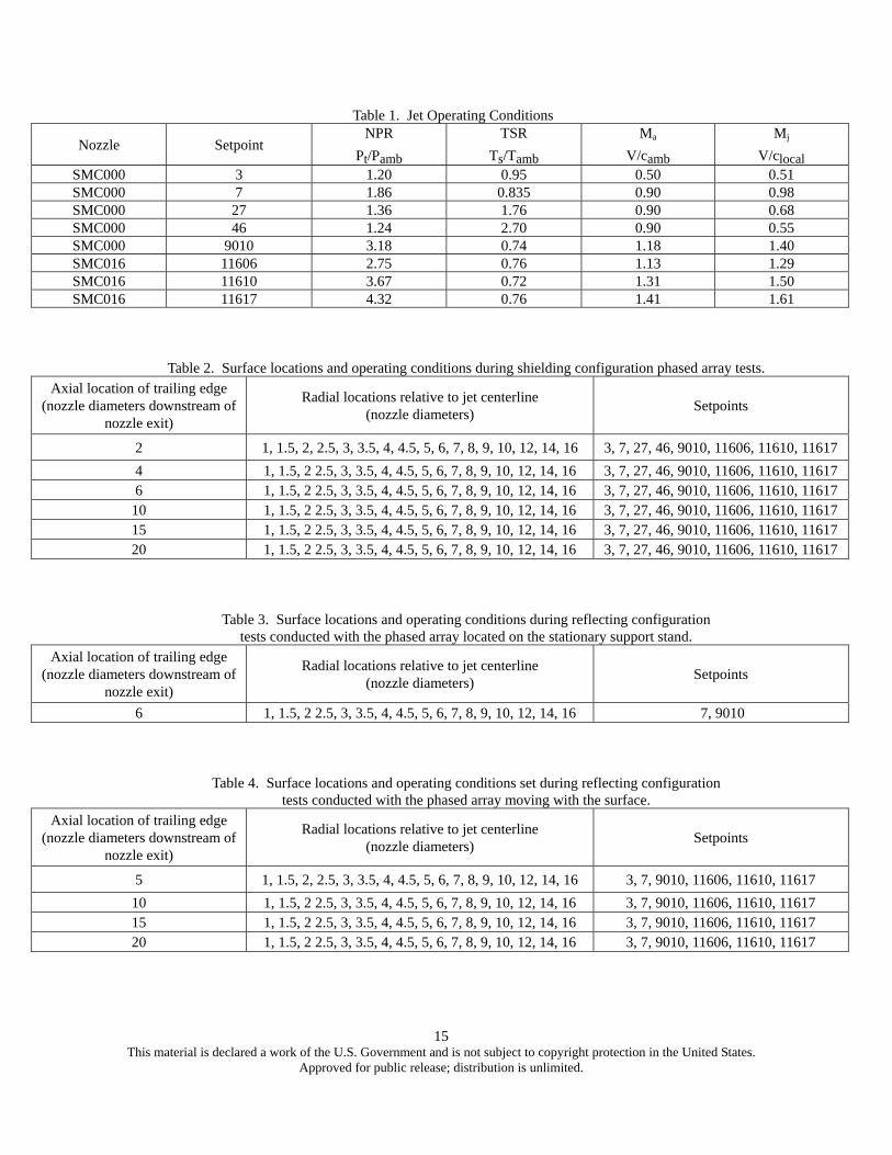
Table 1. Jet Operating Conditions
Nozzle Setpoint NPR
Pt/Pamb
TSR
Ts/Tamb
Ma
V/camb
Mj
V/clocal SMC000 3 1.20 0.95 0.50 0.51 SMC000 7 1.86 0.835 0.90 0.98 SMC000 27 1.36 1.76 0.90 0.68 SMC000 46 1.24 2.70 0.90 0.55 SMC000 9010 3.18 0.74 1.18 1.40 SMC016 11606 2.75 0.76 1.13 1.29 SMC016 11610 3.67 0.72 1.31 1.50 SMC016 11617 4.32 0.76 1.41 1.61
Table 2. Surface locations and operating conditions during shielding configuration phased array tests.
Axial location of trailing edge (nozzle diameters downstream of
nozzle exit)
Radial locations relative to jet centerline (nozzle diameters)
Setpoints
2 1, 1.5, 2, 2.5, 3, 3.5, 4, 4.5, 5, 6, 7, 8, 9, 10, 12, 14, 16 3, 7, 27, 46, 9010, 11606, 11610, 11617
4 1, 1.5, 2 2.5, 3, 3.5, 4, 4.5, 5, 6, 7, 8, 9, 10, 12, 14, 16 3, 7, 27, 46, 9010, 11606, 11610, 11617 6 1, 1.5, 2 2.5, 3, 3.5, 4, 4.5, 5, 6, 7, 8, 9, 10, 12, 14, 16 3, 7, 27, 46, 9010, 11606, 11610, 11617
10 1, 1.5, 2 2.5, 3, 3.5, 4, 4.5, 5, 6, 7, 8, 9, 10, 12, 14, 16 3, 7, 27, 46, 9010, 11606, 11610, 11617 15 1, 1.5, 2 2.5, 3, 3.5, 4, 4.5, 5, 6, 7, 8, 9, 10, 12, 14, 16 3, 7, 27, 46, 9010, 11606, 11610, 11617 20 1, 1.5, 2 2.5, 3, 3.5, 4, 4.5, 5, 6, 7, 8, 9, 10, 12, 14, 16 3, 7, 27, 46, 9010, 11606, 11610, 11617
Table 3. Surface locations and operating conditions during reflecting configuration tests conducted with the phased array located on the stationary support stand.
Axial location of trailing edge (nozzle diameters downstream of
nozzle exit)
Radial locations relative to jet centerline (nozzle diameters)
Setpoints
6 1, 1.5, 2 2.5, 3, 3.5, 4, 4.5, 5, 6, 7, 8, 9, 10, 12, 14, 16 7, 9010
Table 4. Surface locations and operating conditions set during reflecting configuration tests conducted with the phased array moving with the surface.
Axial location of trailing edge (nozzle diameters downstream of
nozzle exit)
Radial locations relative to jet centerline (nozzle diameters)
Setpoints
5 1, 1.5, 2, 2.5, 3, 3.5, 4, 4.5, 5, 6, 7, 8, 9, 10, 12, 14, 16 3, 7, 9010, 11606, 11610, 11617
10 1, 1.5, 2 2.5, 3, 3.5, 4, 4.5, 5, 6, 7, 8, 9, 10, 12, 14, 16 3, 7, 9010, 11606, 11610, 11617 15 1, 1.5, 2 2.5, 3, 3.5, 4, 4.5, 5, 6, 7, 8, 9, 10, 12, 14, 16 3, 7, 9010, 11606, 11610, 11617 20 1, 1.5, 2 2.5, 3, 3.5, 4, 4.5, 5, 6, 7, 8, 9, 10, 12, 14, 16 3, 7, 9010, 11606, 11610, 11617
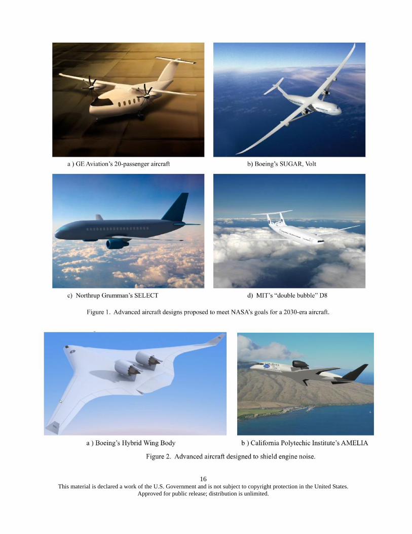
16
This material is declared a work of the U.S. Government and is not subject to copyright protection in the United States. Approved for public release; distribution is unlimited.
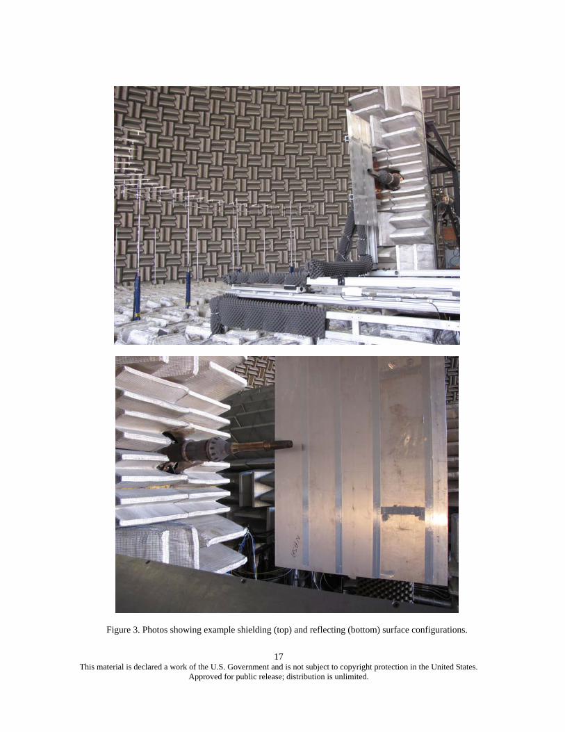
17
This material is declared a work of the U.S. Government and is not subject to copyright protection in the United States. Approved for public release; distribution is unlimited.
Figure 3. Photos showing example shielding (top) and reflecting (bottom) surface configurations.
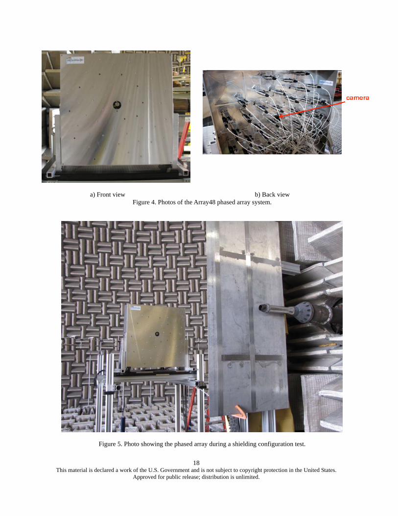
18
This material is declared a work of the U.S. Government and is not subject to copyright protection in the United States. Approved for public release; distribution is unlimited.
a) Front view b) Back view
Figure 4. Photos of the Array48 phased array system.
Figure 5. Photo showing the phased array during a shielding configuration test.
19
This material is declared a work of the U.S. Government and is not subject to copyright protection in the United States. Approved for public release; distribution is unlimited.
Figure 6. Photo showing the phased array mounted on the moveable cart during a reflecting configuration test.
Figure 7. Single microphone spectra (upper left), peak location plot (lower left), 1/12th OB beamform maps (right), and
OASPL beamform map (lower right) for the SMC000 RC nozzle operating at setpoint 3 (Ma=0.50, TSR=0.95)
20
This material is declared a work of the U.S. Government and is not subject to copyright protection in the United States. Approved for public release; distribution is unlimited.
setpoint 3, Ma = 0.50 setpoint 7, Ma = 0.90
Figure 8. Single mic spectra (upper left), peak location plots (upper right), and beamform maps (bottom) for the
SMC000 nozzle at setpoints 3 (Ma=0.50, TSR=0.95) and 7 (Ma=0.90, TSR=0.835).

21
This material is declared a work of the U.S. Government and is not subject to copyright protection in the United States. Approved for public release; distribution is unlimited.
setpoint 27, Ma = 0.90, TSR=1.76 setpoint 46, Ma = 0.90, TSR=2.70
Figure 9. Single mic spectra (upper left), peak location plots (upper right), and beamform maps (bottom) for
the SMC000 nozzle at setpoints 27 (Ma=0.90, TSR=1.76) and 46 (Ma=0.90, TSR=2.70).

22
This material is declared a work of the U.S. Government and is not subject to copyright protection in the United States. Approved for public release; distribution is unlimited.
setpoint 11606, over-expanded, Mj=1.29 setpoint 11610, ideally-expanded, Mj=1.50 setpoint 11617, under-expanded, Mj=1.61 Figure 10. Single mic spectra (upper left), peak location plots (upper right), and 1/12th OB beamform maps (bottom) for SMC016 CD
nozzle at setpoints 11606 (Mj=1.29, TSR=0.76), 11610 (Mj=1.50, TSR=0.72) and 11617 (Mj=1.61, TSR=0.76).
23
This material is declared a work of the U.S. Government and is not subject to copyright protection in the United States. Approved for public release; distribution is unlimited.
Figure 11. BBSN spectral humps predicted using Tam’s model compared with experimental data.
(figure taken from Miller, ref 10)
Figure 12. Peak frequencies (asterisks) corresponding to the two lowest-frequency BBSN humps predicted by Tam’s model overlaid on
top of spectra and peak location plots measured with SMC016 CD nozzle at setpoints 11606 (Mj=1.29) and 11617 (Mj=1.61)

24
This material is declared a work of the U.S. Government and is not subject to copyright protection in the United States. Approved for public release; distribution is unlimited.
Figure 13. Nondimensional peak noise source location plotted
versus nondimensional frequency for each of the seven tested setpoints.
25
This material is declared a work of the U.S. Government and is not subject to copyright protection in the United States. Approved for public release; distribution is unlimited.
Figure 14. Schematic showing jet/surface intersection points for surfaces 1, 2, and 3 jet diameters from the jet centerline and a jet assumed to expand at a 7 angle.
Figure 15. Single mic spectra (upper left), attenuation plots (center left), peak location plot (lower left) and beamform maps (right) for the bare jet and surfaces extending 2, 4, 6, 10, 15, and 20D downstream of nozzle and 3D away from jet centerline
for the SMC000 nozzle at setpoint 7 (Ma=0.90, TSR=0.835).

26
This material is declared a work of the U.S. Government and is not subject to copyright protection in the United States. Approved for public release; distribution is unlimited.
Figure 16. Single microphone spectra (upper left), attenuation plots (center left), peak location plot (lower left) and beamform maps (right) for the bare jet and surfaces extending 2, 4, 6, 10, 15, and 20D downstream of nozzle and 2D away from jet centerline
for the SMC000 nozzle at setpoint 7 (Ma=0.90, TSR=0.835).
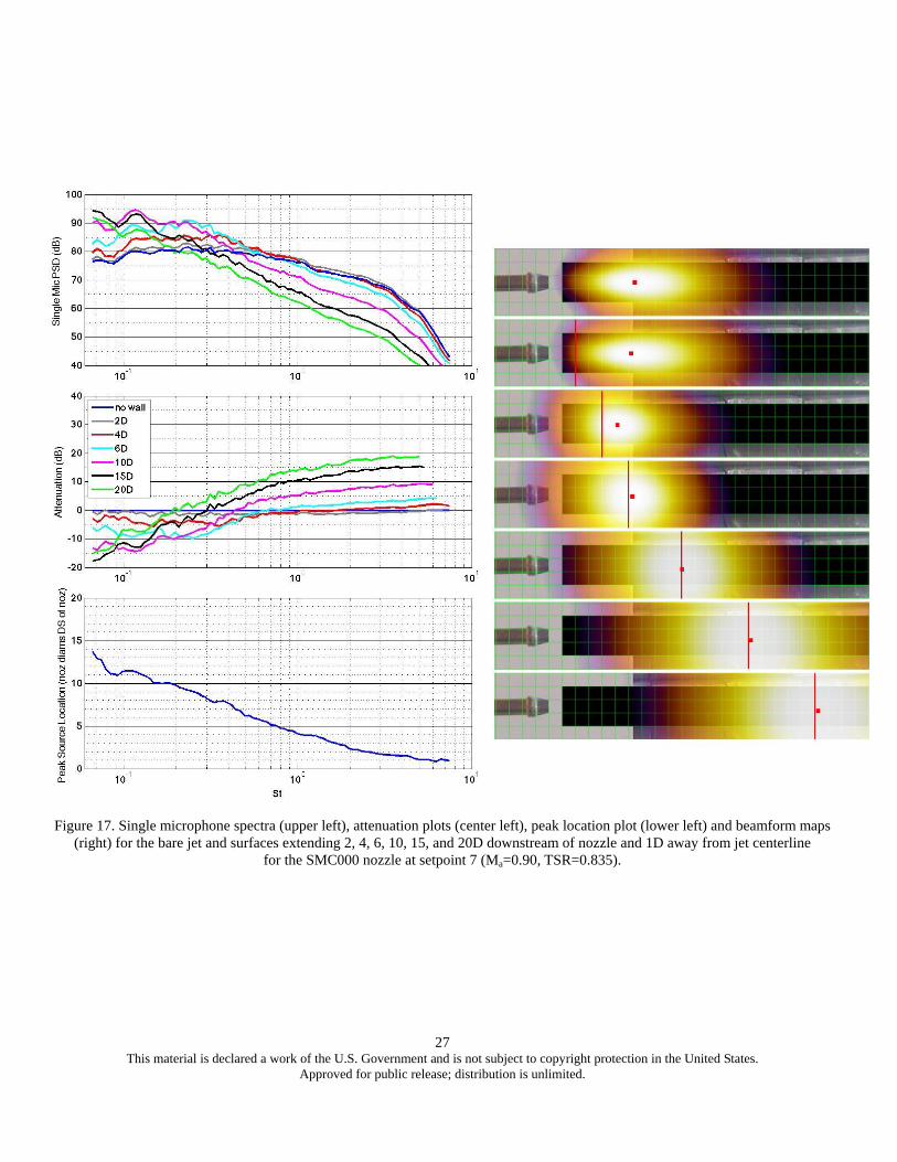
27
This material is declared a work of the U.S. Government and is not subject to copyright protection in the United States. Approved for public release; distribution is unlimited.
Figure 17. Single microphone spectra (upper left), attenuation plots (center left), peak location plot (lower left) and beamform maps (right) for the bare jet and surfaces extending 2, 4, 6, 10, 15, and 20D downstream of nozzle and 1D away from jet centerline
for the SMC000 nozzle at setpoint 7 (Ma=0.90, TSR=0.835).

28
This material is declared a work of the U.S. Government and is not subject to copyright protection in the United States. Approved for public release; distribution is unlimited.
Figure 18. Single mic spectra (upper left), attenuation plots (center left), peak location plot (lower left) and beamform maps (right) for the bare jet and surfaces extending 2, 4, 6, 10, 15, and 20D downstream of nozzle and 3D away from jet centerline for the SMC016
nozzle at the over-expanded setpoint (11606, Mj=1.29, TSR=0.76).
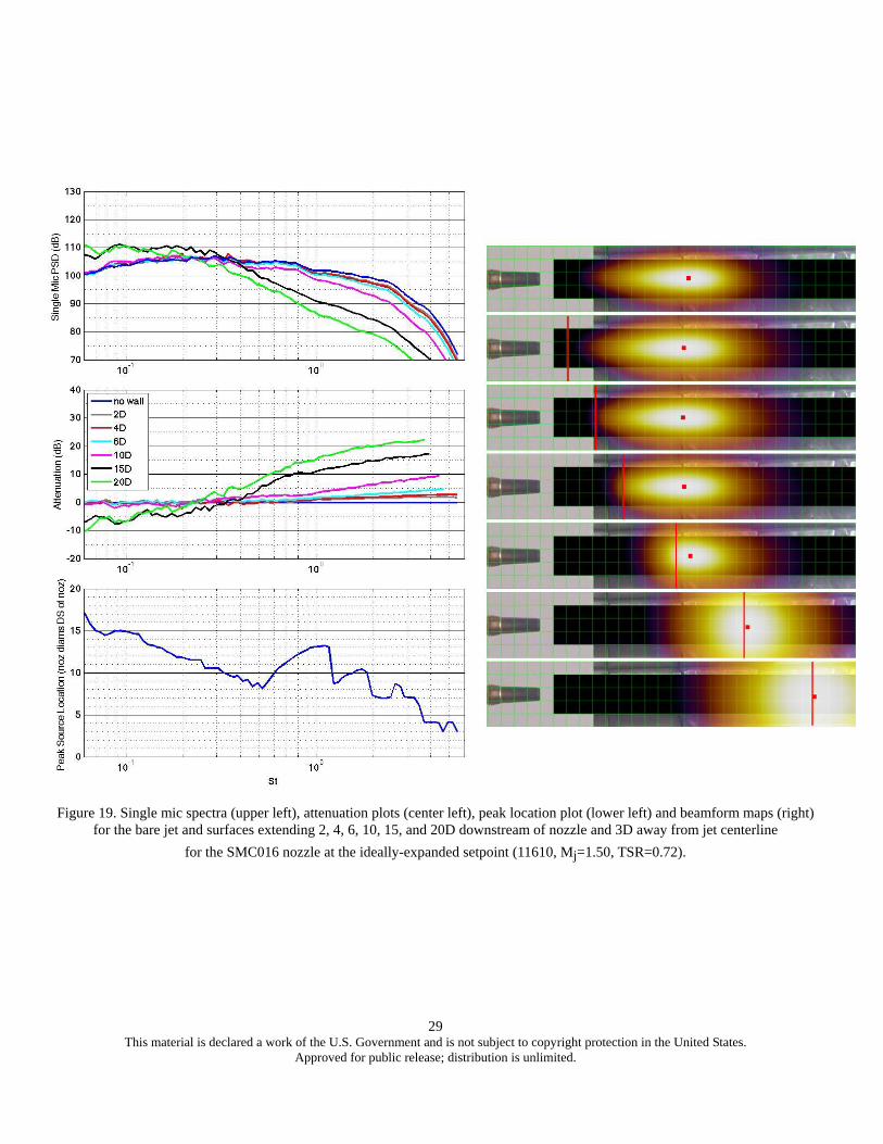
29
This material is declared a work of the U.S. Government and is not subject to copyright protection in the United States. Approved for public release; distribution is unlimited.
Figure 19. Single mic spectra (upper left), attenuation plots (center left), peak location plot (lower left) and beamform maps (right) for the bare jet and surfaces extending 2, 4, 6, 10, 15, and 20D downstream of nozzle and 3D away from jet centerline
for the SMC016 nozzle at the ideally-expanded setpoint (11610, Mj=1.50, TSR=0.72).

30
This material is declared a work of the U.S. Government and is not subject to copyright protection in the United States. Approved for public release; distribution is unlimited.
Figure 20. Single mic spectra (upper left), attenuation plots (center left), peak location plot (lower left) and beamform maps (right) for the bare jet and surfaces extending 2, 4, 6, 10, 15, and 20D downstream of nozzle and 3D away from jet centerline for the SMC016 CD
nozzle at the under-expanded setpoint (11617, Mj=1.61, TSR=0.76).
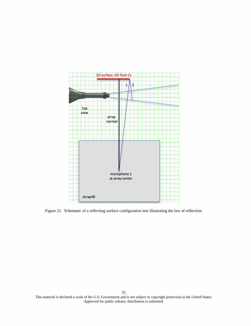
31
This material is declared a work of the U.S. Government and is not subject to copyright protection in the United States. Approved for public release; distribution is unlimited.
Figure 21. Schematic of a reflecting surface configuration test illustrating the law of reflection.

32
This material is declared a work of the U.S. Government and is not subject to copyright protection in the United States. Approved for public release; distribution is unlimited.
Figure 22. Beamform map peak spectra (upper left), single mic spectra (upper right) and beamform maps (bottom) for the bare jet and
the 5D reflecting surface located 4D from the jet centerline for the SMC000 nozzle at setpoint 7. The beamform maps are bare jet (left column), jet/surface combination (center), and surface alone (right).
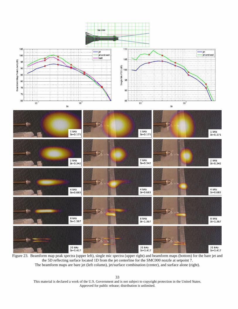
33
This material is declared a work of the U.S. Government and is not subject to copyright protection in the United States. Approved for public release; distribution is unlimited.
Figure 23. Beamform map peak spectra (upper left), single mic spectra (upper right) and beamform maps (bottom) for the bare jet and
the 5D reflecting surface located 1D from the jet centerline for the SMC000 nozzle at setpoint 7. The beamform maps are bare jet (left column), jet/surface combination (center), and surface alone (right).
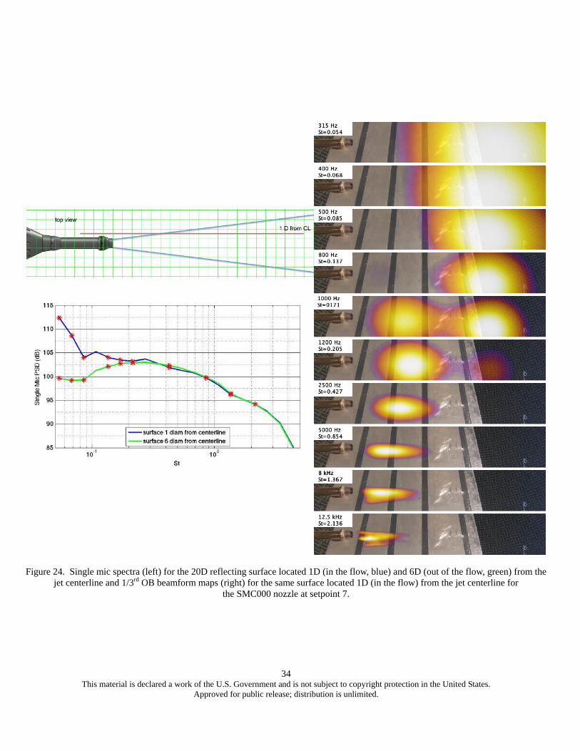
34
This material is declared a work of the U.S. Government and is not subject to copyright protection in the United States. Approved for public release; distribution is unlimited.
Figure 24. Single mic spectra (left) for the 20D reflecting surface located 1D (in the flow, blue) and 6D (out of the flow, green) from the jet centerline and 1/3rd OB beamform maps (right) for the same surface located 1D (in the flow) from the jet centerline for
the SMC000 nozzle at setpoint 7.