1

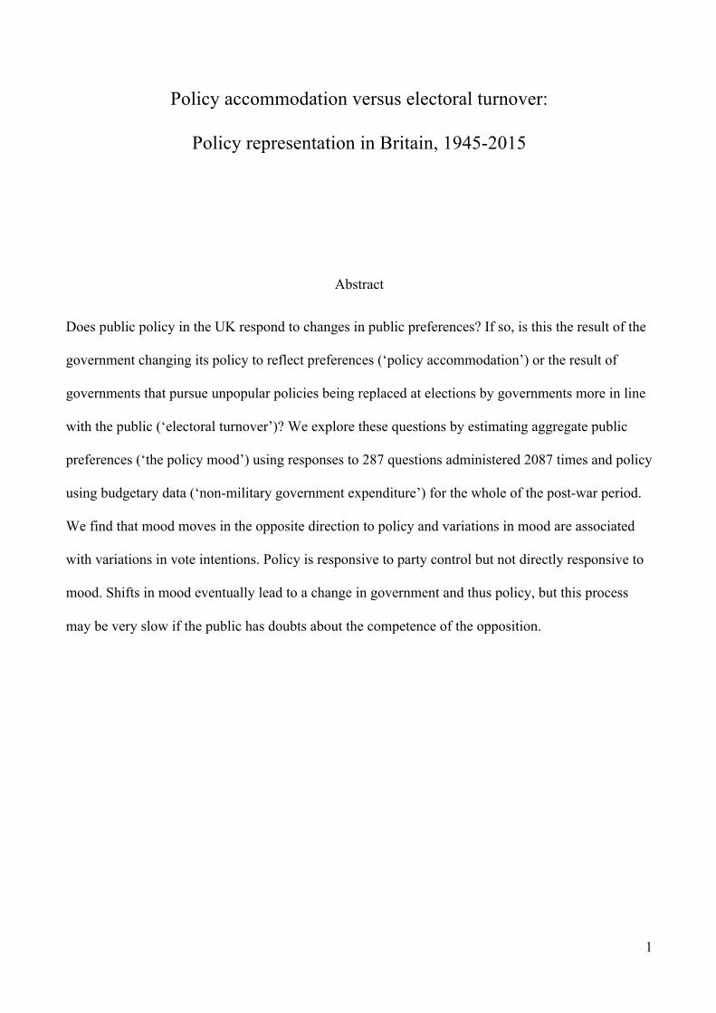
Policy accommodation versus electoral turnover:

Policy representation in Britain, 1945-2015

Abstract

Does public policy in the UK respond to changes in public preferences? If so, is this the result of the

government changing its policy to reflect preferences (‘policy accommodation’) or the result of

governments that pursue unpopular policies being replaced at elections by governments more in line

with the public (‘electoral turnover’)? We explore these questions by estimating aggregate public

preferences (‘the policy mood’) using responses to 287 questions administered 2087 times and policy

using budgetary data (‘non-military government expenditure’) for the whole of the post-war period.

We find that mood moves in the opposite direction to policy and variations in mood are associated

with variations in vote intentions. Policy is responsive to party control but not directly responsive to

mood. Shifts in mood eventually lead to a change in government and thus policy, but this process

may be very slow if the public has doubts about the competence of the opposition.

2

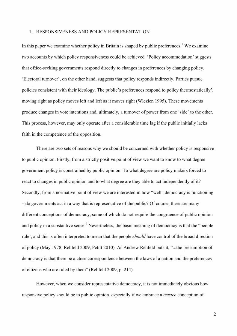
1. RESPONSIVENESS AND POLICY REPRESENTATION

In this paper we examine whether policy in Britain is shaped by public preferences.1 We examine

two accounts by which policy responsiveness could be achieved. ‘Policy accommodation’ suggests

that office-seeking governments respond directly to changes in preferences by changing policy.

‘Electoral turnover’, on the other hand, suggests that policy responds indirectly. Parties pursue

policies consistent with their ideology. The public’s preferences respond to policy thermostatically’,

moving right as policy moves left and left as it moves right (Wlezien 1995). These movements

produce changes in vote intentions and, ultimately, a turnover of power from one ‘side’ to the other.

This process, however, may only operate after a considerable time lag if the public initially lacks

faith in the competence of the opposition.

There are two sets of reasons why we should be concerned with whether policy is responsive

to public opinion. Firstly, from a strictly positive point of view we want to know to what degree

government policy is constrained by public opinion. To what degree are policy makers forced to

react to changes in public opinion and to what degree are they able to act independently of it?

Secondly, from a normative point of view we are interested in how “well” democracy is functioning

– do governments act in a way that is representative of the public? Of course, there are many

different conceptions of democracy, some of which do not require the congruence of public opinion

and policy in a substantive sense.2 Nevertheless, the basic meaning of democracy is that the “people

rule’, and this is often interpreted to mean that the people should have control of the broad direction

of policy (May 1978; Rehfeld 2009, Petitt 2010). As Andrew Rehfeld puts it, “...the presumption of

democracy is that there be a close correspondence between the laws of a nation and the preferences

of citizens who are ruled by them” (Rehfeld 2009, p. 214).

However, when we consider representative democracy, it is not immediately obvious how

responsive policy should be to public opinion, especially if we embrace a trustee conception of

3

representation. If we think that the appropriate form of representation is a delegate model – the

government ought to follow the instructions of the people – and we apply this to the government as a

whole as opposed to individual representatives, then we should expect government policy to follow

public opinion.3 Of course, it is still necessary to interpret what the people’s “instructions” are.4 Even

in this case we might expect the government to follow the will of the people in broad terms rather

than in terms of specific policies. Following Christiano (1996, p.215-7), we might expect the

government to be a delegate in terms of ends, while being a trustee in terms of means.

However, if we endorse a trustee model of representation – representatives are expected to

use their judgment to advance the interests of the people to the best of their ability – then a

considerable amount of slippage between public opinion and policy may be completely acceptable in

a democracy. It is still possible that trusteeship will produce a high degree of responsiveness. If the

people choose trustees whose values and interests align closely with their own, they may choose

policies that naturally track the preferences of the public (what Mansbridge 2003 terms “gyroscopic

representation”). Similarly, trustee representation and popular control could be reconciled through

deliberation and public reason, in what Pettit calls “interpretive representation”.5 On the other hand,

while trustees are expected to act in the interest of the public, they also may choose policies that

differ from what the public wants. If the policies demanded by the public want are impossible or ill-

advised (they do not achieve the ends the public wishes to achieve) then trustee representation will

result in policies that diverge from what the public wants.6

However, it is important not to take this argument too far. While trustee representation allows

for some slippage between public opinion and policy, we should still be concerned if there is a

complete disconnect. If democratic trusteeship allows the public to be completely disregarded, then

there is a danger that it simply becomes a euphemism for benign despotism or paternalism. A trustee,

according to Burke (1777/1963), must make decisions in the interests of the people, and may not

substitute their own interests in place of those of the people. When we observe government policy

4

diverging from public opinion, we are faced with the question as to whether this is the legitimate use

of trusteeship in the interests of the people, or whether the government is substituting its own

interests for those of the people. Lack of policy responsiveness certainly does not prove that there

has been a failure of democratic representation, but it does call for explanation and justification. As

Rehfeld (2009, p. 214) argues, “we must always justify and explain cases in which law deviates from

citizen preferences, whereas no such prima facie justification is required in cases when law conforms

to the preferences and wills of those it governs.”

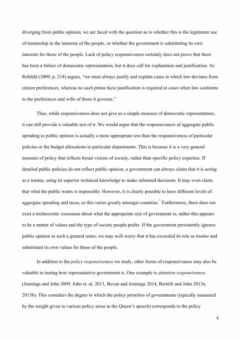
Thus, while responsiveness does not give us a simple measure of democratic representation,

it can still provide a valuable test of it. We would argue that the responsiveness of aggregate public

spending to public opinion is actually a more appropriate test than the responsiveness of particular

policies or the budget allocations to particular departments. This is because it is a very general

measure of policy that reflects broad visions of society, rather than specific policy expertise. If

detailed public policies do not reflect public opinion, a government can always claim that it is acting

as a trustee, using its superior technical knowledge to make informed decisions. It may even claim

that what the public wants is impossible. However, it is clearly possible to have different levels of

aggregate spending and taxes, as this varies greatly amongst countries.7 Furthermore, there does not

exist a technocratic consensus about what the appropriate size of government is; rather this appears

to be a matter of values and the type of society people prefer. If the government persistently ignores

public opinion in such a general sense, we may well worry that it has exceeded its role as trustee and

substituted its own values for those of the people.

In addition to the policy responsiveness we study, other forms of responsiveness may also be

valuable in testing how representative government is. One example is attention responsiveness

(Jennings and John 2009, John et. al. 2013, Bevan and Jennings 2014, Bertelli and John 2013a,

2013b). This considers the degree to which the policy priorities of governments (typically measured

by the weight given to various policy areas in the Queen’s speech) corresponds to the policy

5

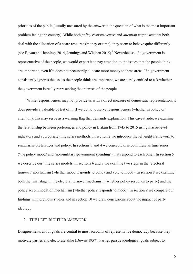
priorities of the public (usually measured by the answer to the question of what is the most important

problem facing the country). While both policy responsiveness and attention responsiveness both

deal with the allocation of a scare resource (money or time), they seem to behave quite differently

(see Bevan and Jennings 2014, Jennings and Wlezien 2015).8 Nevertheless, if a government is

representative of the people, we would expect it to pay attention to the issues that the people think

are important, even if it does not necessarily allocate more money to these areas. If a government

consistently ignores the issues the people think are important, we are surely entitled to ask whether

the government is really representing the interests of the people.

While responsiveness may not provide us with a direct measure of democratic representation, it

does provide a valuable of test of it. If we do not observe responsiveness (whether in policy or

attention), this may serve as a warning flag that demands explanation. This caveat aide, we examine

the relationship between preferences and policy in Britain from 1945 to 2015 using macro-level

indicators and appropriate time series methods. In section 2 we introduce the left-right framework to

summarise preferences and policy. In sections 3 and 4 we conceptualise both these as time series

(‘the policy mood’ and ‘non-military government spending’) that respond to each other. In section 5

we describe our time series models. In sections 6 and 7 we examine two steps in the ‘electoral

turnover’ mechanism (whether mood responds to policy and vote to mood). In section 8 we examine

both the final stage in the electoral turnover mechanism (whether policy responds to party) and the

policy accommodation mechanism (whether policy responds to mood). In section 9 we compare our

findings with previous studies and in section 10 we draw conclusions about the impact of party

ideology.

2. THE LEFT-RIGHT FRAMEWORK

Disagreements about goals are central to most accounts of representative democracy because they

motivate parties and electorate alike (Downs 1957). Parties pursue ideological goals subject to

6

electoral considerations (Strøm 1990). The electorate want governments both to produce policy that

honours their values and govern with competence (Erikson et al. 2002). Preferences and positions

link parties with the electorate and provide the basis for effective communication (Scarbrough 1984).

There are a very large number of issues that people disagree about. If we are to understand the

interaction between parties and the electorate we need to cut away inessential detail (Budge 2006).

Accordingly, we assume that the interaction between parties and the electorate takes place along

single left-right dimension (Downs 1957). The preferences that are of interest to us are those on

which the parties have taken positions. ‘Left’ means those preferences expressed or positions

adopted by Labour. ‘Right’ means those adopted by the Conservatives (Budge and Farlie 1977).

Parties aim to attract voters. They take positions on wide range of issues. Some are enduring.

Some are transient. The ‘core’ issues that divide the major parties relate to economics. Labour has

generally supported ‘more’ government activity, ‘more’ collective action and ‘more’ equality. The

Conservatives have generally supported ‘less’ (Blais et al. 1993). Nevertheless, Labour and the

Conservatives disagree on other issues relating to law and order, individual freedom, the

environment and international affairs. As new issues emerged, the parties have adopted opposing

positions and these have acquired ‘left’ or ‘right’ polarities (Carmines and Stimson 1989). It is usual,

for example, to label support for shorter sentences, equal rights for gays, environment protection and

international co-operation as ‘left-wing’. This enables analysts to use texts to summarise party

positions using both economic and non-economic positions. The MARPOR ‘RILE’ scores, for

example, provide evidence about how parties compete for office (Budge et al. 2001).

There are doubts whether public preferences can be so simplified (Budge 2006). Fortunately, it

is not necessary to resolve the vexing issue of the ‘real’ structure of public preferences here (Stimson

2004). Our purpose is simply to summarise preferences in such a way as to understand the

interaction between parties and the electorate. Accordingly, we focus on the core economic issues

7

that represent the enduring differences between the parties relating to government intervention,

collective action and economic equality (Heath et al. 1994). This decision also simplifies the

measurement of policy since it is difficult – if not impossible – to produce annual measures of policy

that incorporate both economic and non-economic issues using textual data.9

3. MEASURING MACRO-LEVEL PREFERENCES: ANNUAL POLICY MOOD

If we are to analyse responsiveness we need a public preference time series (Erikson et al. 2002).

Micro-level theories provide us with good reasons for believing that we can use preferences across a

wide range of issues to produce an annual indicator of public preferences. Many issues become

‘seemingly related’ and acquire ‘left-right’ polarities (Carmines and Stimson 1989). Since most

people have low levels of political awareness they absorb both ‘left’ and ‘right’ considerations

(Zaller and Feldman 1992). The typical individual is ‘ambivalent’ about issues. Their responses to

questions depend on their predispositions, the issues raised, precise wording and response options

offered. Individual predispositions can be viewed as a running tally of ‘left’ and ‘right’

considerations across all issues. If we could aggregate preferences across both individuals and issues,

this ‘double summation’ would provide an indicator of the electorate’s aggregate (varying) left-right

preferences or ‘policy mood’ (Stimson 1999).

We cannot directly average aggregate responses across survey items. Each survey question

has its own biases as a result of the issues that it engages, precise wording and response options

provided (Zaller and Feldman 1992). Each question has its own metric. Nevertheless, we can use a

method – the dyads ratio algorithm – to find a common metric and then aggregate across issues

(Stimson 1999). Before we outline this method, however, we describe the data at our disposal.

3.1 Data: the preferences database

Responses to a wide range of survey probes reflect left-right preferences. Variations in responses

over time should, therefore, reflect the changing ‘policy mood’ (Stimson, 1999). The raw data to

8

estimate mood are aggregate responses to controversial questions. They require people to ‘choose’

between options, express ‘preferences’, adopt ‘positions’ or take ‘sides’ (Ellis and Stimson 2012).

Since mood is inferred by observing changes between two time points, identical questions

must be asked in at least two separate years to form ‘dyads’ (Stimson, 1999). Items that refer to

particular parties or politicians are excluded from the database, since it is difficult to disentangle

attitudes to these objects from preferences.10 All the data are taken from nationally representative

surveys. In total, the database contains 791 items and 5363 separate readings of preferences.11

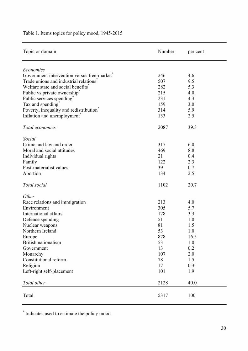
3.2 Content

Our database consists of responses to many controversial issues on which the parties can be expected

to take contrasting positons. Some 287 questions in 2087 separate readings of preferences (39.7 per

cent of the total) relate to ‘core-economic’ domain, including government intervention, trade unions,

public ownership, public spending, taxation, inequality and the trade-off between inflation and

unemployment (see table 1). Another 1102 readings (21 per cent of the total readings) relate to

‘social’ issues. This domain includes crime and law and order, moral and social attitudes, individual

rights, the family and abortion. The ‘other’ category (around 40 per cent of all readings) relate to

diverse issues including immigration, international affairs, defence spending, nuclear weapons,

Northern Ireland, Europe, national sentiment, the monarchy and left-right self-placement.

<Table 1. Topic coverage >

If we were confident that public preferences – like party positions – were undimensional, we

could estimate mood using all the available data. Since we are ignorant of the real structure, we

estimate mood using only items relating to the ‘core economic’ issues. Even after this self-imposed

restriction, however, there here is more than sufficient data to reliably estimate annual mood.

3.3 Coding responses

9

Our focus here is on the ‘core’ left-right issues. Responses are scored from high (most left or Labour)

and to low (most right or Conservative) responses. It is straightforward to code these items since the

parties have taken consistent (opposing) positions.12 Assigning the ‘wrong’ polarities to responses

makes no difference to the estimates of mood – it simply results in negative factor loadings that alert

us to a coding error (Stimson 1999).

All preferences are expressed as an index of preferences:

!"#$%'()*$($*$"+$, = ./0123/0/3/45/6789:./01;<=>?123/0/3/45/67

89:×100

These indexes reflect then balance of left-right preferences on controversial issues. They are

fed into the dyads ratio algorithm in order to estimate mood.

3.4 Method: the dyads ratio algorithm

The raw index of preferences represents the percentage of all substantive responses that are ‘left’.13

Each index is then expressed as a ratio at two time points (years).

Rij=xt+i

xt+j

These dyads have an expected value of 1.0 and can be averaged to produce a rough estimate of

underlying preferences (C1). The algorithm calculates all the possible dyads for each series %1D

iteratively and averages them:14

Pt=xtk

Nk=1

N

Since not all items are equally valid indicators of underlying preferences each series is

weighted by their estimated validity ℎFG.

Pt=hi

2xtkNk=1

h2N

10

Using ratios causes the original metric to be lost. This is reintroduced by a standardization of

the latent scale in terms of the validity-weighted means and standard deviations of the input items

(Stimson 1999). The individual items are scored as per cent left over per cent left plus percent right.

The estimated mood, therefore, has the same interpretation. Fifty is the neutral point. Values above

50 indicate net left preferences and those below 50 indicate net right preferences.

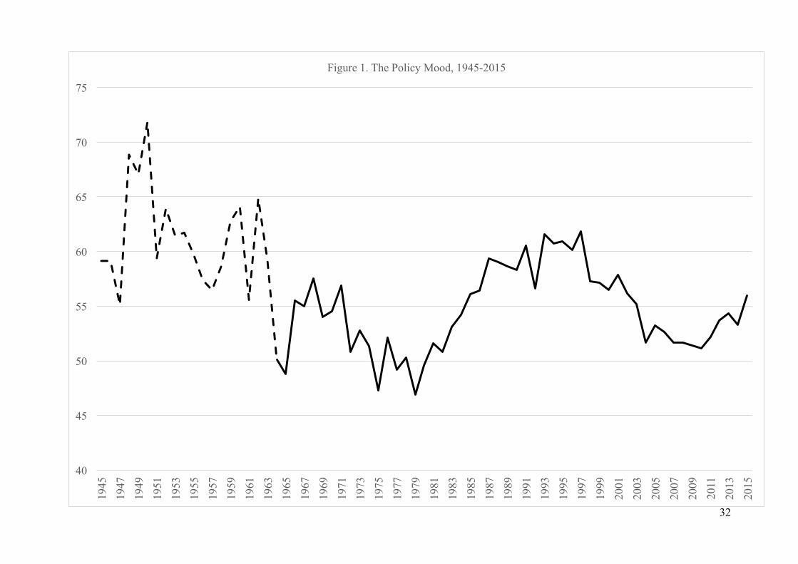
3.5 Estimates of the policy mood

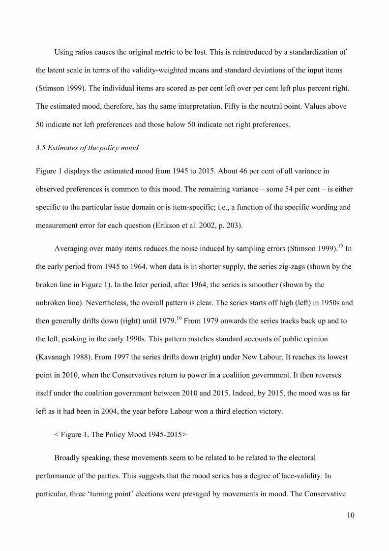
Figure 1 displays the estimated mood from 1945 to 2015. About 46 per cent of all variance in

observed preferences is common to this mood. The remaining variance – some 54 per cent – is either

specific to the particular issue domain or is item-specific; i.e., a function of the specific wording and

measurement error for each question (Erikson et al. 2002, p. 203).

Averaging over many items reduces the noise induced by sampling errors (Stimson 1999).15 In

the early period from 1945 to 1964, when data is in shorter supply, the series zig-zags (shown by the

broken line in Figure 1). In the later period, after 1964, the series is smoother (shown by the

unbroken line). Nevertheless, the overall pattern is clear. The series starts off high (left) in 1950s and

then generally drifts down (right) until 1979.16 From 1979 onwards the series tracks back up and to

the left, peaking in the early 1990s. This pattern matches standard accounts of public opinion

(Kavanagh 1988). From 1997 the series drifts down (right) under New Labour. It reaches its lowest

point in 2010, when the Conservatives return to power in a coalition government. It then reverses

itself under the coalition government between 2010 and 2015. Indeed, by 2015, the mood was as far

left as it had been in 2004, the year before Labour won a third election victory.

< Figure 1. The Policy Mood 1945-2015>

Broadly speaking, these movements seem to be related to be related to the electoral

performance of the parties. This suggests that the mood series has a degree of face-validity. In

particular, three ‘turning point’ elections were presaged by movements in mood. The Conservative

11

victory in 1979, New Labour’s landslide in 1997 and the Tories return to power – as the dominant

party in the coalition in 2010 – all appear to reflect prior movements. Yet some election outcomes do

not seem to be explicable given movements in mood. The October 1974 and 1979 general elections,

for example, produced a Labour victory on the one hand and a Conservative victory on the other,

despite the similar levels of mood. Similarly, the 1992 and 1997 elections produced a Conservative

victory and a Labour landslide, though mood was at much the same level. Other factors – social

change, party positions and assessments of party competence – must be taken into account.

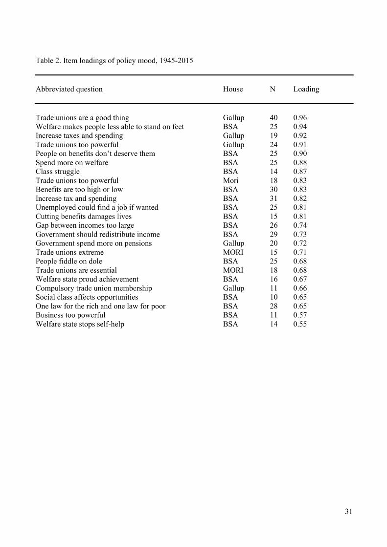
In order to illustrate the content of mood, we briefly examine the factor loadings for

individual items on the estimated mood series. Since there are 287 series, it is not possible to

examine all the loadings. And, since the series vary in length, it would be misleading examine the

loadings for all the individual series. Table 2 displays the loadings for the items that are entered in

the database in at least ten years and load at 0.5 or above.

< Table 2. Items loading on the policy mood>

The items that load on mood relate to trade unions, welfare, tax and spending and inequality.

This is a consequence of our decision to include only the ‘core’ issues. The same items would feature

prominently in the equivalent table if we had estimates the mood using all the preferences data.17

The mood estimated from this larger database, moreover, correlates highly with our mood measure

(Pearson’s R=0.90). These observations do not resolve the issue of the dimensionality of preferences.

They do reassure us that our decision to use only ‘core’ items is not consequential. Averaging a large

number of items produces a robust estimator of preferences.

4. MEASURING ANNUAL MACRO-LEVEL POLICY

In order to assess the interaction between governments and the electorate, it is necessary to develop a

measure of government policy analogous to our measure of mood. ‘Policy’ is a course of action or

the principles adopted by government. It is difficult to summarise because governments take lots of

12

action make many statements of principle. They legislate, enter into treaties, make administrative

decisions, tax and spend and issue statements of intent. It is also difficult to summarise because it can

be indicated by both words (intentions) and deeds (actions and policy delivery).

4.1 Non-military government spending

Spending is a particularly appropriate indicator of delivered policy. It provides a numeraire that gets

to heart of the choice between ‘more’ or ‘less’ (Blais et al. 1996, p. 43). The key indicator of Total

managed expenditure (TME), for example, summarises government activity in an annual time series.

This includes Departmental Expenditure Limits (DELs) that have been allocated to Departments and

Annually Managed Expenditure (AME) that is not controlled by government departments.18

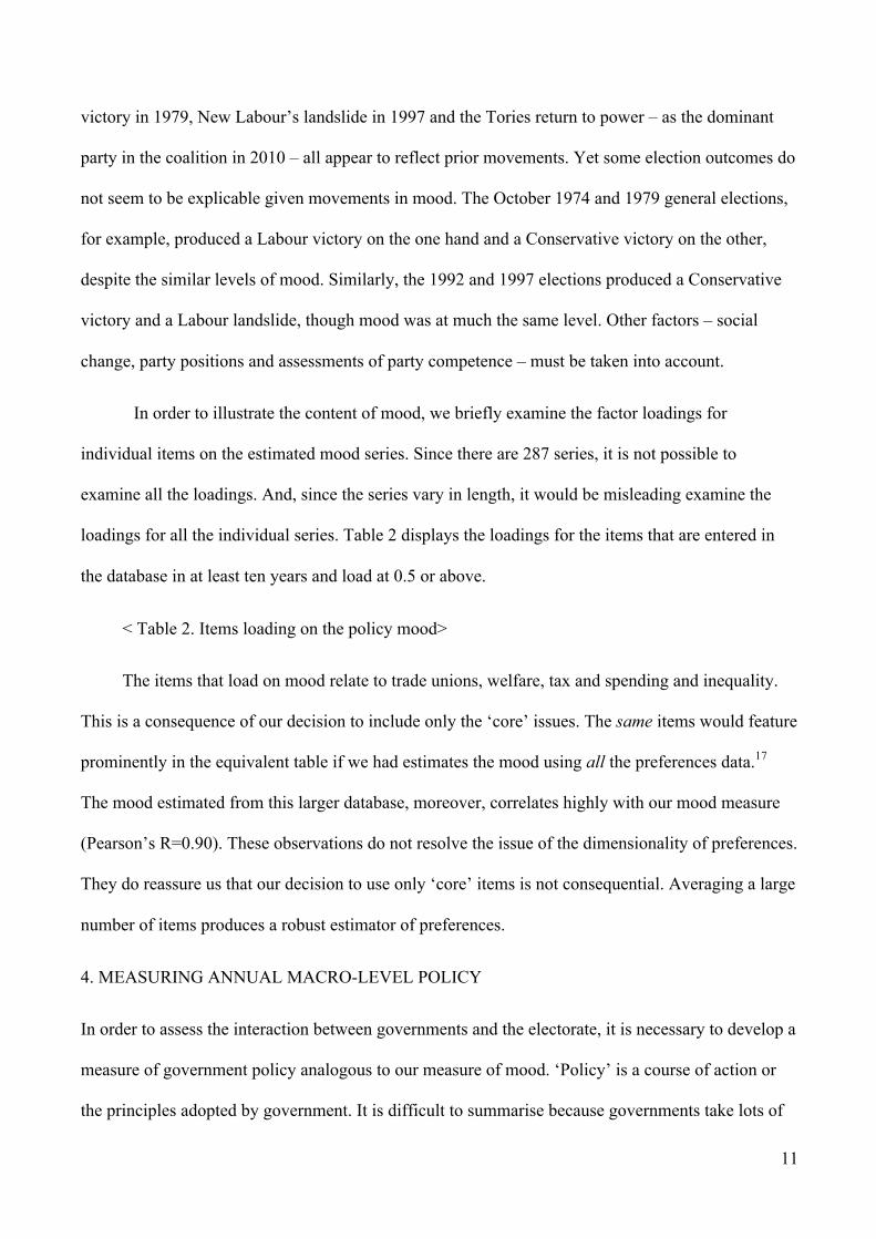
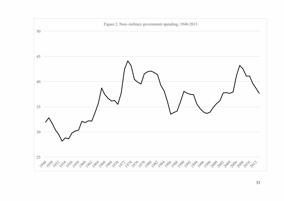
< Figure 2. Non-military government spending, 1948-2013>

The parties’ preferences about spending reflect their ideologies. Labour governments prefer

‘more’ spending on welfare, health and transport. Conservative governments prefer ‘less’. In some

domains, however, these preferences are reversed. The most significant case is defence spending.

This has fluctuated between a high of 9.8 per cent of GDP in 1953 to a low of 2 per cent in 2015.19 In

general, Conservatives prefer more and Labour prefers less spending on defence. Military spending,

moreover, is influenced by perceptions of threat and is less responsive to domestic politics. In order

to provide a more accurate indicator of domestic policy, we subtract defence as a percentage of GDP

spending from TME to produce Non-Military Government Expenditure (NMGE).

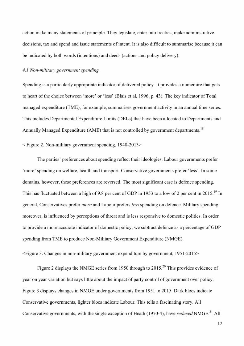
<Figure 3. Changes in non-military government expenditure by government, 1951-2015>

Figure 2 displays the NMGE series from 1950 through to 2015.20 This provides evidence of

year on year variation but says little about the impact of party control of government over policy.

Figure 3 displays changes in NMGE under governments from 1951 to 2015. Dark blocs indicate

Conservative governments, lighter blocs indicate Labour. This tells a fascinating story. All

Conservative governments, with the single exception of Heath (1970-4), have reduced NMGE.21 All

13

Labour governments have increased it. Our characterisation of elections as a choice between ‘more’

with Labour and ‘less’ with the Conservatives has a degree of face validity.

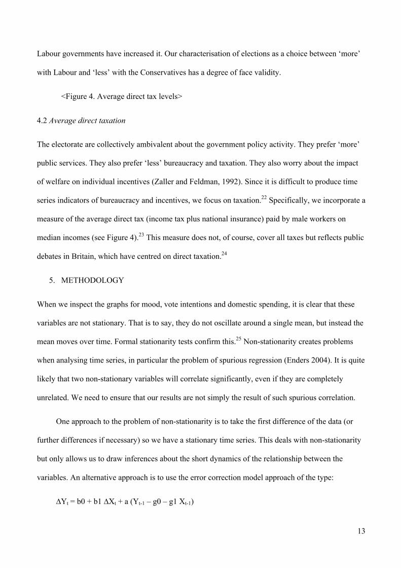
<Figure 4. Average direct tax levels>

4.2 Average direct taxation

The electorate are collectively ambivalent about the government policy activity. They prefer ‘more’

public services. They also prefer ‘less’ bureaucracy and taxation. They also worry about the impact

of welfare on individual incentives (Zaller and Feldman, 1992). Since it is difficult to produce time

series indicators of bureaucracy and incentives, we focus on taxation.22 Specifically, we incorporate a

measure of the average direct tax (income tax plus national insurance) paid by male workers on

median incomes (see Figure 4).23 This measure does not, of course, cover all taxes but reflects public

debates in Britain, which have centred on direct taxation.24

5. METHODOLOGY

When we inspect the graphs for mood, vote intentions and domestic spending, it is clear that these

variables are not stationary. That is to say, they do not oscillate around a single mean, but instead the

mean moves over time. Formal stationarity tests confirm this.25 Non-stationarity creates problems

when analysing time series, in particular the problem of spurious regression (Enders 2004). It is quite

likely that two non-stationary variables will correlate significantly, even if they are completely

unrelated. We need to ensure that our results are not simply the result of such spurious correlation.

One approach to the problem of non-stationarity is to take the first difference of the data (or

further differences if necessary) so we have a stationary time series. This deals with non-stationarity

but only allows us to draw inferences about the short dynamics of the relationship between the

variables. An alternative approach is to use the error correction model approach of the type:

∆Yt = b0 + b1 ∆Xt + a (Yt-1 – g0 – g1 Xt-1)

14

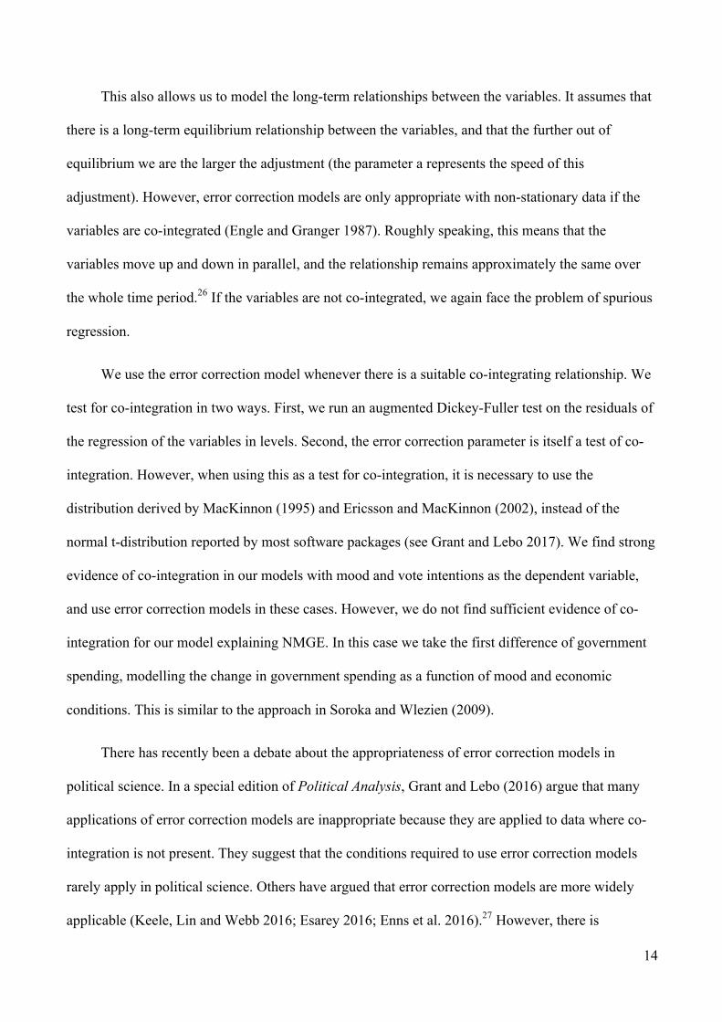
This also allows us to model the long-term relationships between the variables. It assumes that

there is a long-term equilibrium relationship between the variables, and that the further out of

equilibrium we are the larger the adjustment (the parameter a represents the speed of this

adjustment). However, error correction models are only appropriate with non-stationary data if the

variables are co-integrated (Engle and Granger 1987). Roughly speaking, this means that the

variables move up and down in parallel, and the relationship remains approximately the same over

the whole time period.26 If the variables are not co-integrated, we again face the problem of spurious

regression.

We use the error correction model whenever there is a suitable co-integrating relationship. We

test for co-integration in two ways. First, we run an augmented Dickey-Fuller test on the residuals of

the regression of the variables in levels. Second, the error correction parameter is itself a test of co-

integration. However, when using this as a test for co-integration, it is necessary to use the

distribution derived by MacKinnon (1995) and Ericsson and MacKinnon (2002), instead of the

normal t-distribution reported by most software packages (see Grant and Lebo 2017). We find strong

evidence of co-integration in our models with mood and vote intentions as the dependent variable,

and use error correction models in these cases. However, we do not find sufficient evidence of co-

integration for our model explaining NMGE. In this case we take the first difference of government

spending, modelling the change in government spending as a function of mood and economic

conditions. This is similar to the approach in Soroka and Wlezien (2009).

There has recently been a debate about the appropriateness of error correction models in

political science. In a special edition of Political Analysis, Grant and Lebo (2016) argue that many

applications of error correction models are inappropriate because they are applied to data where co-

integration is not present. They suggest that the conditions required to use error correction models

rarely apply in political science. Others have argued that error correction models are more widely

applicable (Keele, Lin and Webb 2016; Esarey 2016; Enns et al. 2016).27 However, there is

15

agreement that if the data is non-stationary, error correction models are only appropriate where co-

integration is present. We only use error correction models where there is clear evidence of co-

integration, using the tests recommended by Grant and Lebo (2016).28

6 DOES MOOD RESPOND TO POLICY?

We now examine the electoral turnover mechanism in two stages. In this section we examine

whether public preferences (as measured by the policy mood) respond to policy. In the next section

we examine whether vote intentions respond to mood.

Previous research has established that preferences for policy (Rij) reflect the difference between

ideal points (Pi) and actual policy (Pj) (Wlezien 1995).

Rij = Pi - Pj

When actual policy exceeds the ideal (Pi>Pj) then Rij>0 and the electorate signal their

preference for less. When policy is less than ideal (Pi<Pj) then Rij<0 and the electorate signal their

preferences for ‘more’ activity. Preferences act like a ‘thermostat’. The same logic applies to mood.

As spending increases the public want less. Accordingly:

H1. The electorate move to the right as NMGE increases

The electorate prefer lower levels of direct tax taxation. Accordingly:

H2. The electorate move to the right as average income tax increases.

Government activity is not the only influence on mood. Exogenous changes in the economy

can also shape preferences. Increasing unemployment, for example, will lead the electorate to prefer

more activity in order to reduce unemployment.29 Thus, independently of policy, the electorate will

shift left as unemployment increases. These considerations suggest:

H3. The electorate move to the left as unemployment increases.

16

We model mood using an error correction model. Given that our variables are non-stationary

and there is a co-integration relation between the dependent and independent variables, this is

appropriate.30 The dependent variable is mood. The independent variables are lagged values of

average income tax levels, NMGE and unemployment.

Table 3 displays the estimated coefficients from the error correction model. The estimated

error correction rate (0.81) implies that over 80 per cent of any deviation of preferences from the

target rate in either direction is corrected within one year. The coefficients provide support for H1

and H2. The statistically significant negative coefficients for long-term effects for both NMGE (H =-

0.59) and average income tax rates (H =-0.37) clearly suggest thermostatic relationships. There is

also short-term relationship between ∆%and ∆J for NMGE (H =-0.59). As government activity

increases, the electorate moves right and, as government activity decreases, it moves left. The long-

term effect for unemployment also provides support for H3 (H =0.86).31

<Table 3 What drives policy mood>

This evidence confirms the thermostatic hypothesis (Wlezien 1995). The electorate responds to

both policy and economic conditions. Changing preferences communicate a desire to reduce

government activity when ‘too hot’ and increase it when ‘too cold’.32 This is evidence of the first

link in the ‘chain of responsiveness’ and representation. It is characteristic of both electoral turnover

and policy accommodation mechanisms (Powell 2000). We now examine the next link in the

electoral turnover mechanism: whether votes respond to mood.

7. POLICY MOOD AND VOTE INTENTIONS

Before proceeding, we must note that preferences are not the only the plausible influences on vote:

they are also influenced by long-term partisanship (Clarke et al. 2004), policy moderation (Nagel and

Wlezien 2011) and evaluations of competence (Green and Jennings 2010).33 From this list of ‘usual

suspects’ we only have indicators of annual party competence. These are estimated using the dyads-

17

ratio-algorithm and drawing on responses to survey questions about which party is best able to deal

with any particular issue (Green and Jennings, 2010).34 Unfortunately, we do not have annual

indicators of partisanship or party position at our disposal. Partisanship was rarely measured in the

1950s and 1960s. The ‘traditional’ measure of partisanship is, moreover, influenced by the same

short-term factors that it is assumed to shape (Clarke et al. 2004). Accordingly, our vote intention

model tests two hypotheses:

H4. Increasing evaluations of Labour’s competence increase Labour vote.

H5. Leftwards shifts in the mood increase Labour vote

Once again we use an error correction model, as there is co-integration between the

dependent and independent variables.35 Table 4 assesses the relationship between annual Labour vote

intentions, mood and evaluations of Labour competence between 1951 and 2015. The error

correction term is significant and correctly signed (H =-0.57) suggesting that 57 per cent of any

deviation of preferences from the target rate is corrected within one year. Both the long and short-

term coefficients for competence are significant and correctly signed (H =0.62 and H = 0.74

respectively) providing support for H4. Crucially, the coefficient for the long-term effect of mood is

significant (H = 0.17). As the mood moves left, Labour vote intentions increases.36 H5 is confirmed.

<Table 4. What drives annual vote intentions>

These results suggest that variations in mood have an electoral impact net of evaluations of

competence. This provides some evidence for another step in the electoral turnover mechanism. The

effect of competence is greater than mood. As a result, a move towards (say) the left in mood will

not produce an increase in support for the Labour Party if there is even a small loss of confidence in

the competence of the Labour Party.

8 PARTY IDEOLOGY, MOOD AND POLICY REPRESENTATION

18

We now examine whether policy responds to party incumbency or mood. If NMGE responds to party

incumbency, this will confirm that governments pursue policy consistent with their ideology and

provide evidence in favour of the electoral turnover mechanism. If it responds to mood, this will

provide evidence in favour of the policy accommodation mechanism

We did not find an appropriate co-integrating relationship, and so did not use an error

correction model. Instead, we took the first difference of NMGE and regressed lagged mood, the

change in unemployment and the change in inflation on this. This is similar to the approach in

Soroka and Wlezien (2009). This specification is theoretically appropriate because our

operationalization of mood is intrinsically thermostatic. Respondents are typically not asked to name

their ideal level of government spending on a programme; they are asked whether spending is too

high, too low or about right. Left-wing mood means that the public demands more public spending

than at present. As a result, we would expect left-wing mood to produce an increase in spending.

If electoral turnover was producing representation, who is in government should ‘make a

difference’. Labour governments should spend more than Conservative governments other things

being equal.37 Accordingly, the electoral turnover model suggests:

H6. Labour governments have higher levels of NMGE than Conservative.

If policy accommodation was producing representation, NMGE should respond to the

preferences communicated by variations in mood. The government could anticipate that the

electorate will punish it if it does not deliver policies compatible with the mood of the electorate.

This will lead to the government reacting to the current policy mood, perhaps with a lag. However, it

could also anticipate what the mood the public will have at the time of the next election. If it is able

to do this, then the future mood will have an effect on current policy. We test both possibilities.

H7. Increases in the policy mood should increase NMGE.

19

Table 5 displays the coefficients generated by five models. Firstly we model NMGE as

function of mood in the previous period, the change in unemployment and the previous period’s

inflation rate. In the second model we take into account policy mood in each of the previous four

years, to explore the effect of a change in mood over a five-year parliament. We then add political

variables to each of these models, producing models 3 and 4. We include a variable representing

whether Labour was in government, together with a dummy variable for 1974. Public spending in

that year increased by 4.5% of GDP as a result of factors such as the oil crisis and the miners’ strike

(see Figure 2). Finally, in model 5 we consider whether the government’s anticipation of the mood at

the time of the next election has an effect on policy. We add a variable for the level of mood

forecasted in the next period using the data available to that point.38

<Table 5. What drives government spending, 1949-2013?>

The first thing that is apparent from inspecting the five models is that mood has no significant

effect on domestic spending – indeed the estimated coefficients are very close to zero. This is true

even if we add the effects of four lags of mood. The mood forecasted for the next period also does

not have a statistically significant effect. These results are inconsistent with H8. There is no support

for the idea that movements in mood leads to an increase in NMGE, whether we control for the

effect of the party in government or not. There is no support for the policy accommodation

mechanism.

By contrast, the coefficient for the party in government does have a significant effect. As

importantly, this effect is substantially very significant. According to our models, Labour

governments raise domestic spending by between 0.51 and 0.67% of GDP per year more than

Conservative governments. Thus we find strong support for Hypothesis 8. Essentially parties keep

pursuing the policies they are committed to, regardless of changes in public mood.

20

The effects of the various control variables are as expected. A change in unemployment leads

to a very substantial increase in public spending. This is not unsurprising as unemployment directly

increases spending on unemployment benefit and other social programmes. Inflation leads to small,

but significant fall in spending. Again this is what we would expect as inflation makes it easier for

governments to cut programmes by simply not fully indexing them. The dummy variable for 1974

also has the expected effect.

These findings confirm the impression in Figure 5. Simply put, ‘party matters’ (Blais, et al.

1996). Labour’s reputation as the party of ‘big’ or ‘bigger’ government party is based on fact. So is

the Conservative party’s reputation as the party of ‘small’ or ‘smaller’ government. This part of the

‘electoral turnover’ mechanism works very well – the parties offer voters a consistent and reliable

choice between ‘more’ or ‘less’ government. We would expect that in the long-run changes in mood

will lead to a change in government, which will in turn lead to a change in policy in line with public

preferences. However, as we saw in the last section, mood only has a weak effect on party support,

and this can easily be overwhelmed by considerations of competence.39 Although we would expect

‘the electoral turnover’ mechanism to work in the long-run, it may well fail for a considerable time if

voters believe the opposition to be incompetent.

9 DISCUSSION

The proposition that the electorate’s preferences help provide direction to policy seems implausible

given what is known about the ‘typical voter’ (Achen and Bartels 2016). Yet, in Britain, as in the US,

“our knowledge of the individual voter turns out not to be a reliable guide for generalising to the

electorate and its role in democratic politics” (Erikson et al. 2002 p. 3). Variations in mood

communicate real preferences and influence vote decisions.40 These ‘messages’, however, are not

acted on. Representation can only work by turning over power from ‘one side’ to ‘the other’. The

parties play their part by reliably pursuing policies consistent with their left-right ideology.

21

Our findings contrast with other studies that suggest that there is a degree of policy

accommodation. Soroka and Wlezien’s 2009 study, for example, uncovered evidence of policy

representation in specific domains such as defence, social affairs, health and education between 1978

and 1995.41 Preferences in those domains responded thermostatically to spending. Policy, in turn,

responded to preferences. Soroka and Wlezien measure preferences using responses to specific

Gallup questions about whether spending in those domains should be increased or decreased and

they measure policy by spending in the same domains. This approach assumes that variations in

these individual series reflect preferences and spending in a particular domain.42 It seems wholly

reasonable to suggest, however, that preferences in those domains may also partly reflect the general

policy mood and overall spending. The observed ‘thermostatic’ effect may well reflect the

diminishing marginal utility of spending in that domain but it may also reflect the electorate’s

ambivalence to government activity – in particular its aversion to taxes and borrowing. This is

particularly the case in those areas of government activity that account for a large share of

spending.43 It might be informative, therefore, to repeat Soroka and Wlezien’s analyses controlling

for the policy mood (less those items relating to a specific domain) and overall spending.44 The

overall budget constraint must also impose constraints on spending and responsiveness.

Our findings also contrast with Erikson et al.’s study of responsiveness and representation in

the United States, which concluded that policy was sensitive to preferences. This study, like our own,

used mood to measure preferences.45 Policy was measured, however, using congressional rating

scales and roll call outcomes (Erikson et al. 2002 p 294-5).46 Analogous indicators are not available

in the British case. Even if such measures were available, they would have less validity. Party

discipline is strong and there are few defections on ideological votes (Cowley 2002). It may be that

the US system of checks and balances ensures that preferences are taken into consideration (Powell

2000). The same may be true of ‘consensus’ democracies (Lijphart, 1999). There is clearly a need for

collaborative research along the lines of the Comparative Agendas Project (Baumgartner et al. 2009).

22

Our results also differ greatly from those of Hakhverdian (2010), who argues that there is

high degree of policy responsiveness in the British case, and furthermore that this is the result of

“rational anticipation”, a process roughly equivalent to what we refer to as “policy accommodation”.

However, the different results are unsurprising when we consider how Hakhverdian measures

government policy. Like us, Hakhverdian seeks to explain how left- or right-wing government policy

is. However, unlike us he does not measure this in terms of government actions, such as tax and

spending decisions, but rather by the content of budget speeches, using the Wordscores programme

(Laver et al. 2003).47 It seems that when public opinion moves to the left, governments include more

left-wing themes in their budget statements, but do not change tax or spending behaviour.

Our findings also appear to contrast with the policy agendas literature (Jennings and John

2009, John et. al. 2013, Bevan and Jennings 2014, Bertelli and John 2013a, 2013b). This literature

demonstrates that government attention (as measured by the content of the official policy speeches)

is responsive to the public’s policy agenda (as measured by responses to the most important issue or

most important problem question). This contrast is, however, more apparent than real, as quite

different things are being measured. British governments appear to be responsive in the sense of

addressing the issues that the public thinks are important. However, when it comes to decisions about

the level of spending, they follow their party ideologies.

10 CONCLUSIONS

Our results suggest that domestic spending policy is not responsive to mood and is driven,

instead, by economic conditions and party control (Strøm 1990; Blais et al. 1996). That is to say, we

do not find evidence of “policy accommodation” by governments – governments pursue policies

consistent with their ideologies unaffected by changes in public opinion. The unresponsiveness of

governments seems surprising given the ‘power hoarding’ nature of the British constitution (King

2007). British governments are guaranteed a parliamentary majority. The government at Westminster

23

is not constrained by federal structures. The principle of parliamentary sovereignty, moreover,

implies that the courts do not have power of constitutional review. British governments have the

power to either respond to or anticipate the impact of preferences – but they do not appear to so.

We do find evidence that public opinion may affect policy through the mechanism of

“electoral turnover”. We find that changes in policy mood affect voting intentions. If policy mood

moves against the ideology of the current government, it will lose support and eventually be replaced

by a government whose ideology reflects the public’s mood. This should lead to a correction in

policy in line with public opinion. However, this process may take a considerable amount of time.

We find that the effect of policy mood on voting intentions is not as strong as the effect of people’s

assessment of government competence. If the public lacks faith in the competence of the opposition,

the government may retain power for a considerable amount of time, even though it may be moving

policy in the opposite direction the public wants.

One reason for our findings may be that the ‘mandate’ from the previous general election has

greater moral force than the requirement to adjust policies to current opinion. If a strategy of policy

accommodation were followed, moreover, it would erode a party’s reputation for reliability and

responsibility (Downs 1957). Governments may follow their ideological impulses to maintain

appeals to members, donors or core voters (Jacobs and Shapiro 2000). Trimming policy to reflect the

‘feedback’ from public preferences may create intra-party tensions (Budge et al. 2010). Conservative

governments that increase taxes, for example, will outrage business interests and the middle class.

Labour governments that cut spending will antagonise trade unions and public sector workers. Policy

may be responsive to majority opinion within governing parties (Hussey and Zaller 2011).

Even if governing parties were willing – in principle – to respond to mood, they may not be

able to detect it. Evidence about public preferences largely comes from snapshots of opinion. Viewed

in cross-section, however, preferences are characterised by considerable ambivalence. People often

24

appear to take ‘different sides’ on the same issue and different ‘sides’ on ‘seemingly-related’ issues

(Stimson 2004). The typical snapshots of preferences on diverse issues may communicate no clear

signal. Indeed, the sheer amount of data may produce considerable uncertainty about ‘what the

public want ‘(Jacobs and Shapiro 2000; Druckman and Jacobs 2006). The mood is only uncovered

once issues are standardised in terms of left and right and then aggregated (Converse 1990). It is

understandable that governments fall back on ideology (Budge 1994).

Given this uncertainty about what people want, it seems only reasonable to suggest that

politicians will select evidence or interpret trends in ways that are politically congenial. Ideology

provides the emotional basis for the sort of ‘motivated reasoning’ (Epley and Giolvich 2016).

Comments such as ‘it’s not what we are hearing on the doorstep’ may reflect either unconscious

biases or wilful ignorance but both result in a failure to ‘receive’ discomforting feedback (Kingdon

1967). Finally, even if governments can ‘hear’ the change of mood and even if they are prepared to

act on it, they may believe that other factors – such as the ‘costs of ruling’ will lead to their

inevitable defeat (Naanstead and Paldam 2007). If governments believe that the swings of the

pendulum operate independently of policy they may well fall back on their ideology (Budge 1994).

25

References

Achen, Christopher H. and Larry M. Bartels. 2016. Democracy for Realists: Why Elections Do Not Produce Representative Government. Princeton, N.J: Princeton University Press.

Bartle, John; Sebastian Dellepiane Avellaneda and James A. Stimson. 2011.‘The moving centre: Preferences for government activity in Britain, 1950-2005’. British Journal of Political Science, 41, 259-85.

Baumgartner Frank; Christoffer Green-Pedersen and Bryan D. Jones, eds,. 2009. Comparative Studies of Policy Agendas. London: Routledge.

Beetham, David and Stuart Weir. 1999. Political Power and Democratic Control in Britain. London: Routledge.

Benoit, Kenneth and Michael Laver. 2006. Party Policy in Modern Democracies. London: Routledge.

Bertelli, Anthony, and Peter John. 2013. ‘Public Policy Investment: Risk and Return in British Politics’, British Journal of Political Science, 43, 741-773.

Bevan, Shaun, and Will Jennings. 2013. ‘Representation, agendas and institutions’, European Journal of Political Research, 53, 37-56.

Blais, Andre, Donald Blake; Stephane Dion. 1996. ‘Do parties make a difference? A reappraisal’, American Journal of Political Science, 40, 514-520.

Blais, Andre´ Donald Blake and Stephane Dion. 1993. ‘Do parties make a difference? Parties and the Size of Government in Liberal Democracies’, American Journal of Political Science, 37, 40–62.

Budge, Ian and Denis Farlie. 1977. Voting and Party Competition. London: Wiley.

Budge, Ian; Hans Dieter Klingemann, Andrea Volkens, Judith Bara and Eric Tanenbaum. 2001. Mapping Policy Preferences: Estimates for Parties, Electors, and Governments 1945-1998. Oxford: Oxford University Press.

Budge, Ian; Michael D. MacDonald and Lawrence Ezrow. 2010. ‘Ideology, Party Factionalism and Policy Change: An integrated dynamic theory’. British Journal of Political Science, 40, 781-804.

Budge, Ian. 1994. ‘A new spatial theory of party competition: Uncertainty, ideology and policy equilibria viewed comparatively and temporally’, British Journal of Political Science, 24, 443–467.

Budge, Ian. 2006. ‘Identifying ideologies and locating parties’, in Ian Katz and William Crotty, eds, Handbook of Party Politics, Beverley Hills: Sage Publications.

Burke, Edmund. 1777 / 1963. Letter to the Sheriffs of Bristol. In Edmund Burke: Selected Writings and Speeches, edited by P. Stanlis. New York: Anchor Books

Butler, David E. and Donald Stokes. 1974. Political Change in Britain: The Evolution of Political Preference. London. Macmillan.

Carmines, Edward G. and James A. Stimson. 1989. Issue Evolution: Race and the Transformation of American Politics. Cambridge: Cambridge University Press.

Clarke, Harold, Marianne Stewart, David Sanders and Paul Whiteley. 2004. Political Choice in Britain. Cambridge: Cambridge University Press.

26

Christiano, Thomas. 1996. The Rule of the Many: Fundamental Issues in Democratic Theory. Boulder: Westview Press.

Converse, Philip E. 1990. ‘Popular representation and the distribution of information’, in John Ferejohn and James Kuklinski, eds, Information and Democratic Processes. Urbana: University of Illinois Press.

Cowley, Philip. 2002. Revolts and Rebellions: Parliamentary Voting Under Blair. London: Politico’s.

Dahl, Robert. 1956. A Preface to Democratic Theory. Chicago: University of Chicago Press.

Dahl, Robert. 1956. A Preface to Democratic Theory. Chicago: University of Chicago Press.

Dalton, Russell J., David M. Farrell and Ian McAllister. 2011. ‘The dynamics of political representation’, in Martin Rosema, Bas Denters and Kees Arts, eds. How Democracy Works: Political Representation and Policy Congruence in Modern Societies. Amsterdam: Pallas Publications.

De Boef, Suzanna and Luke Keele. 2008. ‘Taking time seriously’, American Journal of Political Science, 52, 184–200.

Downs, Anthony.1957. An Economic Theory of Democracy. New York: Harper & Row.

Druckman, James N. and Lawrence R. Jacobs. 2006. ‘Lumpers and splitters: The public pinion information that politicians collect and use’. Public Opinion Quarterly, 70, 453-76.

Duverger, Maurice. 1954. Political Parties. New York: Wiley.

Ellis, Christopher and James A. Stimson. 2012. Political Ideology in America. Cambridge: Cambridge University Press.

Enders, Walter. 2004. Applied Econometric Time Series. Hoboken, N.J: John Wiley & Sons.

Engle, Robert F., and C.W.J Granger. 1987. ‘Co-Integration and Error Correction: Representation, Estimation, and Testing’, Econometrica, 55, 251-276.

Enns, Peter K., Nathan J. Kelly, Takaaki Masaki, and Patrick C. Wohlfarth. 2016. ‘Don’t jettison the general error correction model just yet: A practical guide to avoiding spurious regression with the GECM’. Research and Politics, 1-13.

Epley, Nicholas and Thomas Gilovch, 2016. ‘The mechanics of motivated reasoning’, Journal of Economic Perspectives, 30, 133-40.

Ericsson, Neil R., and James G. MacKinnon. 2002. ‘Distributions of Error Correction Tests for Cointegration’, Econometrics Journal, 5, 285-318.

Erikson, Robert S.; Michael D. MacKuen and James A. Stimson. 2002. The Macro Polity. Cambridge: Cambridge University Press.

Esarey, Justin. 2016. ‘Fractionally Integrated Data and the Autodistributed Lag Model: Results from a Simulation Study’, Political Analysis, 24, 42-49.

Fishkin, James. 1995. The Voice of the People: Public Opinion and Democracy. New Haven: Yale University Press.

Grant, Taylor, and Matthew J. Lebo. 2016. ‘Error Correction Methods with Political Time Series’, Political Analysis, 24, 3-30.

27

Green, Jane and Will Jennings. 2012. ‘Valence as macro-competence: An analysis of mood in party competence evaluations in Great Britain’, British Journal of Political Science, 42, 311–343.

Hakhverdian, Armen. 2010. ‘Political Representation and its Mechanisms: A Dynamic Left-Right Approach for the United Kingdom, 1976-2006’, British Journal of Political Science, 40, 835-56.

Heath, Anthony, Geoffrey Evans and Jean Martin. 1994. ‘The measurement of core beliefs and values: The development of balanced socialist/laissez faire and libertarian/ authoritarian scales’, British Journal of Political Science, 24, 115–138.

Hussey, Wesley and John R. Zaller, 2011. ‘Who do parties represent?’ in Peter K. Enns and Christopher Wlezien, eds, Who Gets Represented? New York: Russell Sage Foundation.

Jacobs, Lawrence R. and Robert Y. Shapiro. 2000. Politicians Don't Pander: Political Manipulation And The Loss Of Democratic Responsiveness. Chicago: Chicago University Press.

Jennings, Will and Christopher Wlezien. 2015. ‘Preferences, Problems and Representation’, Political Science Research & Methods, 3, 659-81.

Jennings, Will, and Peter John. 2009. ‘The Dynamics of Political Attention: Public Opinion and the Queen's Speech in the United Kingdom’, American Journal of Poitical Science, 53(4), 838-854.

John, Peter, Anthony Michael Bertelli, William J. Jennings, and Shaun Bevan. 2013. Policy agendas in British politics, Comparative studies of political agendas series. Basingstoke: Palgrave MacMillan.

Johnson, Paul, Frances Lynch and John Geoffrey Walker. 2005. ‘Income tax and elections in Britain, 1950-2001’, Electoral Studies, 24, 393-408.

Johnston, Ron, Charles Pattie, Danny Dorling and David Rossiter. 2012. From votes to seats: The operation of the UK electoral system since 1945. Manchester: Manchester University Press.

Kavanagh, Dennis.1988. Thatcherism and British Politics: The end of consensus? Oxford: Oxford University Press.

Keele, Luke, Suzanna Linn, and Clayton McLaughlin Webb. 2016. ‘Treating Time with All Due Seriousness’, Political Analysis, 24, 31-41.

Kingdon, John W. 1967. ‘Politicians beliefs about voters’. American Political Science Review, 61, 137-45.

King, Anthony and Robert J. Wybrow. 2000. British Public Opinion, 1937-2000: The Gallup Polls. London: Politicos.

King, Anthony. 2007. The British Constitution. Oxford: Oxford University Press.

King, Gary, Robert O Keohane and Sindney Verba. 1994. Designing Social Inquiry: Scientific Inference in Qualitative Research. Princeton, N.J: Princeton University Press.

Kingdon, John W. 1984. Agendas, Alternatives and Public Policy. Boston, Mass.: Little Brown.

Laver, Michael, Kenneth Benoit and John Garry. 2003. ‘Extracting policy positions from political texts using words as data’, American Political Science Review, 97, 311-331.

Lijphart, Arend. 1975. The Politics of Accommodation. Berkeley: University of California Press.

Lijphart, Arend. 1975. The Politics of Accomodation. Berkeley: University of California Press.

28

Lijphart, Arend. 1977. Democracy in Plural Societies. New Haven: Yale University Press.

Lijphart, Arend. 1977. Democracy in Plural Societies. New Haven: Yale University Press.

Lijphart, Arend. 1999. Patterns of Democracy: Government Forms and Performance in Thirty-Six Countries. New Haven, CT: Yale University Press.

Lowe, Will. 2008. ‘Understanding wordscores’, Political Analysis 16, 356-71.

MacKinnon, James G. 1994. ‘Asymptotic Distribution Functions for Unit-Root and Cointegration Tests’. Journal of Business & Economic Statistics, 12(2), 167-176.

Mansbridge, Jane. 2003. Rethinking Representation. American Political Science Review 97:515-528.

May, John D. 1978. ‘Defining democracy: A bid for coherence and consensus’, Political Studies, 26, 1–14.

McDonald, Michael D. and Ian Budge. 2005. Elections, Parties, Democracy: Conferring the Median Mandate. Oxford: Oxford University Press.

McGann, Anthony. 2014. ‘Estimating the political center from aggregate data: An item response theory alternative to the Stimson dyad ratios algorithm’, Political Analysis, 22, 115-29.

Naanstead, Peter and Martin Paldam. 2002. ‘The costs of ruling’, in Han Dorussen and Michael Taylor, eds, Economic Voting. London: Routledge. pp. 17-44.

Nagel, Jack H. and Christopher Wlezien. 2010. ‘Centre-party strength and major party divergence in Britain, 1945-2005’, British Journal of Political Science, 40, 279-304.

OECD. 2017. Governments at a Glance. Paris: OECD Publishing. https://data.oecd.org/gga/general-government-spending.htm.

Page, Benjamin I. and Robert Y. Shapiro. 1992. The Rational Public: Fifty Years of Trends in Americans’ Policy Preferences. Chicago: The University of Chicago Press.

Petitt, Philip. 2010. Varieties of Public Representation. In Political Representation, edited by I. Shapiro, S. C. Stokes, E. J. Wood and A. S. Kirshner. Cambridge: Cambridge University Press.

Powell, G. Bingham. 2000. Elections as Instruments of Democracy: Majoritarian and Proportional Systems. Yale: Yale University Press.

Przeworski, Adam. 1999. Minimalist Conception of Democracy: A Defense. In Democracy's Value, edited by I. Shapiro and C. Hacker-Cordòn. Cambridge: Cambridge University Press.

Rehfeld, Andrew. 2009. ‘Representation Rethought: On Trustees, Delegates, and Gyroscopes in the Study of Political Representation and Democracy’, American Political Science Review 103, 214-230.

Riker, William. 1982. Liberalism Against Populism: A Confrontation Between the Theory of Democracy and the Theory of Social Choice. San Francisco: Freeman.

Rose, Richard. 1980. Do Parties Make a Difference? London: Macmillan.

Scarbrough, Elinor. 1984. Political Ideology and Voting Behaviour: An exploratory study. Oxford: Clarendon Press.

Schumpeter, Joseph. 1942. Capitalism, Socialism & Democracy. New York: Harper & Brothers.

Soroka, Stuart N. and Christopher Wlezien. 2009. Degrees of Democracy: Politics, Public Opinion, and Policy. Cambridge: Cambridge University Press.

29

Soroka, Stuart N., Christopher Wlezien and Iain McLean. 2006. ‘Public expenditure in the UK: How measures matter’, Journal of the Royal Statistical Society Series A, 166, 255-71.

Soroka, Stuart Neil, and Christopher Wlezien. 2009. Degrees of democracy: politics, public opinion, and policy. Cambridge; New York: Cambridge University Press.

Stimson, James A. 1999. Public Opinion in America: Moods, Cycles and Sings. Boulder, CO: Westview Press.

Stimson, James A. 2004. Tides of Consent: How Public Opinion Shapes American Politics. Cambridge: Cambridge University Press.

Stimson, James; Michael MacKuen and Robert Erikson. 1995. ‘Dynamic representation’, American Political Science Review, 89, 543-65.

Stokes, Donald E. 1963. ‘Spatial models of party competition’, American Political Science Review, 57, 368-77.

Strøm, Kaare. 1990. ‘A behavioural theory of competitive political parties’, American Journal of Political Science. 34, 565-98.

Weber, Max. 1921 / 1978. Economy and Society: An Outline of Interpretive Sociology. Vol. 1. Berkeley: University of California Press.

Weber, Max. 1921/1978. Economy and Society: An Outline of Interpretive Sociology. Vol. 1. Berkeley: University of California Press.

Wildavsky, Aaron. 1964. The Politics of the Budgetary Process. Boston: Little, Brown.

Wlezien, Christopher. 1995 ‘The public as thermostat: Dynamics of preferences for spending’, American Journal of Political Science, 39, 981-1000

Zaller, John R. and Stanley Feldman. 1992. ‘A simple theory of the survey response: Answering questions versus revealing preferences’, American Journal of Political Science, 36, 579-6

30

Table 1. Items topics for policy mood, 1945-2015 Topic or domain Number per cent Economics Government intervention versus free-market* 246 4.6 Trade unions and industrial relations* 507 9.5 Welfare state and social benefits* 282 5.3 Public vs private ownership* 215 4.0 Public services spending* 231 4.3 Tax and spending* 159 3.0 Poverty, inequality and redistribution* 314 5.9 Inflation and unemployment* 133 2.5 Total economics 2087 39.3 Social Crime and law and order 317 6.0 Moral and social attitudes 469 8.8 Individual rights 21 0.4 Family 122 2.3 Post-materialist values 39 0.7 Abortion 134 2.5 Total social 1102 20.7 Other Race relations and immigration 213 4.0 Environment 305 5.7 International affairs 178 3.3 Defence spending 51 1.0 Nuclear weapons 81 1.5 Northern Ireland 53 1.0 Europe 878 16.5 British nationalism 53 1.0 Government 13 0.2 Monarchy 107 2.0 Constitutional reform 78 1.5 Religion 17 0.3 Left-right self-placement 101 1.9 Total other 2128 40.0 Total 5317 100

* Indicates used to estimate the policy mood

31

Table 2. Item loadings of policy mood, 1945-2015 Abbreviated question House N Loading Trade unions are a good thing Gallup 40 0.96 Welfare makes people less able to stand on feet BSA 25 0.94 Increase taxes and spending Gallup 19 0.92 Trade unions too powerful Gallup 24 0.91 People on benefits don’t deserve them BSA 25 0.90 Spend more on welfare BSA 25 0.88 Class struggle BSA 14 0.87 Trade unions too powerful Mori 18 0.83 Benefits are too high or low BSA 30 0.83 Increase tax and spending BSA 31 0.82 Unemployed could find a job if wanted BSA 25 0.81 Cutting benefits damages lives BSA 15 0.81 Gap between incomes too large BSA 26 0.74 Government should redistribute income BSA 29 0.73 Government spend more on pensions Gallup 20 0.72 Trade unions extreme MORI 15 0.71 People fiddle on dole BSA 25 0.68 Trade unions are essential MORI 18 0.68 Welfare state proud achievement BSA 16 0.67 Compulsory trade union membership Gallup 11 0.66 Social class affects opportunities BSA 10 0.65 One law for the rich and one law for poor BSA 28 0.65 Business too powerful BSA 11 0.57 Welfare state stops self-help BSA 14 0.55

32

40

45

50

55

60

65

70

7519

45

1947

1949

1951

1953

1955

1957

1959

1961

1963

1965

1967

1969

1971

1973

1975

1977

1979

1981

1983

1985

1987

1989

1991

1993

1995

1997

1999

2001

2003

2005

2007

2009

2011

2013

2015

Figure 1. The Policy Mood, 1945-2015

33

25

30

35

40

45

50

Figure 2. Non--military government spending, 1948-2013

34

-6

-4

-2

0

2

4

6

8

10

1951-1964 1964-1970 1970-1974 1974-1979 1979-1997 1997-2010 2010-2015

Figure 3. Changes in non-military government expenditure by government, 1951-2013

35

10

15

20

25

30

35

Figure 4. Average rates of direct tax, 1949-2013

36

Table 3. What drives the policy mood? (Error correction model, 1948-2013) Error correction -0.81*** t = 6.75

(0.12) McKinnon p<0.01 critical t value: 4.23

Unemploymentt-1 Long-term 0.86***

(0.21) Short-term 0.59

(0.10)

Average direct tax t-1 Long-term -0.37**

(0.15) Short-term -0.11

(0.35)

Domestic spending t-1

Long-term -0.45***

(0.16) Short-term -0.59***

(0.29) N 63 Breusch-Godfrey 0.03 Adjusted R2 0.44 Root MSE 2.66 Augmented Dickey-Fuller value for integrating equation: -4.30 (lag order 3) *** ***=p<0.01, ** =p<0.05 * =p<0

37

Table 4. What drives annual vote intentions? (Error correction model of Labour vote intentions, 1951-2015) Error correction -0.57*** t = 4.75 (0.12) McKinnon p<0.01 critical t value: 3.29 Mood t-1 Long-term 0.17**

(0.08) Short-term 0.06

(0.10)

Macro-competence t-1

Long-term 0.62***

(0.17) Short-term 0.74***

(0.11)

Constant -7.60*

(4.40) N 64 Breusch Godfrey 2.34 Adjusted R2 0.52 Root MSE 2.24 Augmented Dickey-Fuller value for integrating equation: -4.27 (lag order 3)***

***=p<0.01, ** =p<0.05 * =p<0.1

38

Table 5. What drives annual policy? (Modelling domestic government expenditure, 1949-2013) Model 1 Model 2 Model 3 Model 4 Model 5 Mood t-1 -0.03 -0.07 0.00 -0.04 -0.41 (0.04) (0.06) (0.04) (0.05) (0.73) Mood t-2 -0.05 0.00 -0.17 (0.06) (0.05) (0.33) Mood t-3 0.05 0.01 -0.07 (0.06) (0.05) (0.17) Mood t-4 0.05 0.04 -0.01 (0.05) (0.04) (0.10) Forecasted mood 0.68 (1.32) Sum of lags and -0.01 0.02 0.02 forecast (mood) (0.04) (0.04) (0.04) ∆Unemployment 0.74*** 0.69*** 0.80*** 0.78*** 0.76*** (0.23) (0.24) (0.20) (0.21) (0.21) Inflationt-1 -0.08* -0.08* -0.09** -0.09** -0.08** (0.05) (0.05) (0.04) (0.04) (0.04) Labour in govt. 0.67** 0.60* 0.51 (0.32) 0.34 (0.38) 1974 dummy 4.64*** 4.65*** 4.70*** (1.18) (1.21) (1.23) Constant 2.40 1.31 0.37 -0.60 -1.01 (2.33) (2.54) (2.15) (2.34) (2.48) N 64 64 64 64 64 Adj. R2 0.12 0.12 0.34 0.33 0.32 MSE 1.33 1.33 1.15 1.16 1.17

***=p<0.01, ** =p<0.05 * =p<0.1

39

1 ACKNOWLEDGEMENTS

2 For example, there are “minimalist” theories of democracy, which argue that the value of democracy is simply the discipline imposed on governments by the fact they can be replaced (Weber 1921 / 1978; Schumpeter 1942; Riker 1982). Pzweworski (1999) goes as far as to argue that even the random replacement of governments could bring many of the benefits of democracy. Other theories of democracy are strictly procedural, arguing that democracy should be defined in terms of the fariness of the institutions, rather than its policy outcomes. The “populist theory of democracy” in Dahl’s Preface to Democratic Theory is of this kind (Dahl 1956, ch.2).

3 If representatives act as delegates for separate constituencies, we may not observe responsiveness to public opinion as a whole. For example, delegates who are strictly bound by the instructions of their constituents may lack the discretion necessary to reach the compromises needed to pass any legislation at all.

4 Of course, the public does not in general issue explicit instructions. Rather, we need to infer the intentions of the public from election results. For example, parties may offer electoral programmes and pledges, and the public may endorse them by electing the party (what Mansbridge 2003 refers to as “promissory representation”.) Alternatively, governments could observe public opinion and react to what the public wants, anticipating that the electorate will punish it at the next election if it does not (“anticipatory representation” in Mansbridge’s terminology).

5 Petitt (2010) rejects the idea that public opinion exists exogenously and controls policy, and argues that a trustee conception of representation is inevitable. However, he argues that public opinion and policy correspond to one another in a democracy because both are determined by the same process of deliberation and public reason. Indeed Petitt (2010, 82) argues that the Westminster system is responsive to public opinion precisely because the representatives behave as trustees

6 We might also consider the standard proposed by Fishkin (1995), who argued that representatives should adopt the policies the public would choose if they were properly informed.

7 In 2015 government spending as percentage of GDP in OECD countries varied from 29% in Ireland to 57% in Finland (OECD 2017).

8 Bevan and Jennings (2014) find that while government attention (measured by either mentions in the Queens speech or legislation) does respond to the public’ s assessment of problems, government spending does not in a statistically significant way. Jennings and Wlezien (2015) show that the public perception of a problem being important does not in general correlate with a public demand for more money to be spent on the issue.

9 See Hakhverdian (2011) for such an attempt.

10 Questions that refer to ‘the government’ are a special case. Where the question refers to government in the abstract it is retained. Where it refers to the incumbents, it is not included.

11 We cannot be claim that we found all the data. We can claim that we used all the data that we could find. The series vary greatly in length. The longest Gallup series on whether ‘trades unions are a good thing’ spans some 45 years and is entered in the database some 58 times. Many others span just two years. The longest series relate to the core issues.

40

12 It is not difficult to code responses items as left and right. The exceptions relate to technological issues such as those relating to genetics on which the parties have not taken positions.

13 The mood can also be estimated by McGann’s (2014) estimated based on item-response theory. The two methods produce very similar results.

14 The algorithm estimates dyads both forwards and backwards and averages the two.

15 The policy mood series can be smoothed using an exponential operator. All the models here use unsmoothed mood.

16 The series bounces up in the late 1940s – probably a result of the thinness of the data. This has no consequences for our analyses. The mood models are estimated from 1948; the vote intentions models from 1951. Bi-annual estimates of the mood produce essentially identical results.

17 The additional items that would meet joint requirements would include items relating to the European Union, left-right self-placement, environmentalism and post-materialism.

18 See the Glossary in the Public Finances Data Bank: http://budgetresponsibility.org.uk/docs/dlm_uploads/PSF_aggregates_databank_September_2016.xls

19 Data from Stockholm International Peace Research Institute (SIPRI): https://www.sipri.org/databases/milex

20 The NMGE series starts in 1951 because the SIPRI database starts then. This is also convenient since it misses out the major period of demilitarisation 1945-50.

21 The Heath government started off by cutting spending but was forced to increase as a result of domestic opposition and the oil-price shocks. Since there was a change of government following the February 1974 election, the end point for the Heath government and the start date for the Wilson government is 1973.

22 In principle, we could incorporate ONS indicator of public sector current receipts (PSCR). This indicator is highly correlated, however, with TME.

23 Direct taxes include income tax and national insurance. Estimates to 2005 were produced by Frances Lynch at the University of Westminster (Johnson et al., 2005). This has been updated to 2013 by the authors using the same data sources.

24 This is despite the fact that income tax generates only £182 billion of the £721 billion (25 per cent) of total revenue in 2016/17. See H. M. Treasury, Budget 2016.

25 The augmented Dickey-Fuller statistics (lag order 3) for the three dependent variables were as follows: Policy mood -2.02 (p=0.57); Vote intentions -2.43 (p=0.40); Domestic spending -1.93 (p=0.60). In all cases the null hypothesis of a non-stationary unit root process cannot be rejected.

26 Formally this requires that when the variables are regressed, the error term is stationary.

27 For example, Keele, Lim and Webb (2016) follow Deboef and Keele (2008) in arguing that error correction models can be applied to stationary data, while Esarey (2016) argues that they can usefully be applied to data generated by a partially differenced process.

41

28 A further objection that could be made to our use of error correction models based on the work of Grant and Lebo (2016) is that our data is not really unit-root given that our variables are bounded. They argue that fractionally differenced models are more appropriate in these cases. However, none of our variables come close to reaching their theoretical bounds. Esarey (2016) shows that the amount of data required to reliably estimate a fractionally differenced process is far larger than the 64 years of data we have, and also shows that an error correction model can provide a useful approximation to a fractionally differenced process when co-integration is present.

29Similarly, inflation may lead the electorate to prefer less activity. Inflation is not statistically significant in the mood models and is omitted. This is the result of its high correlation with NMGE (Pearson’s R=0.60, between 1948 and 2014).

30 The augmented Dickey-Fuller score (lag level 3) for the equation in levels is -4.30. Thus, the null hypothesis of non-stationarity in the error term is rejected at the 1% level, indicating that co-integration is present. The value of the error correction term is -0.81 with a standard error of 0.12 and thus a t-value of 6.75. The 1% critical t-value for using this parameter as co-integration test with 64 observations and three variables is 4.23 (calculated from Ericsson and MacKinnon 2002). Thus we conclude co-integration is present.

31 The effects for unemployment and spending reported here are generally stronger than those reported in Bartle et al. (2011a). This is probably because this estimate of mood is only based on the core economic items and because government spending is measured by NMGE rather than TME.

32 This is consistent with Stimson’s (1999) core finding that cycles occur between policy mood and government activity.

33 Policy moderation is defined in terms of the distance between the major party and the Liberal Democrats (or predecessors) in Nagel and Wlezien (2011).

34 Assessments of party competence are estimated using Gallup, Ipsos-Mori and YouGov data gathered by the authors, separately from Green and Jennings (2011).

35 The augmented Dickey-Fuller score (lag level 3) for the equation in levels is -4.27. Thus, the null hypothesis of non-stationarity in the error term is rejected at the 1% level, indicating that co-integration is present. The value of the error correction term is -0.57 with a standard error of 0.12 and thus a t-value of 4.75. The 1% critical t-value for using this parameter as co-integration test with 64 observations and three variables is 3.29 (calculated from Ericsson and MacKinnon 2002). Thus we conclude co-integration is present.

36 Mood does not appear to influence Conservative or Liberal Democrat vote intentions. It should be noted that mood is significant in Labour vote models for general elections (N=16) where controls are imposed for Labour’s position (as represented by the RILE scores), a count variable (capturing unmeasured variables) and evaluations of competence.

37 Between 1945 and 2010 there were a total of eight turnovers of power (1945, 1951, 1964, 1970, February 1974, 1979, 1997 and 2010). The turnovers in 1951 and 1964 occurred late in the year, so in those years Labour are treated as the incumbents in 1951 and the Conservatives are treated as the incumbents in 1964. The turnover in February 1974 took place in February 1974 took place in early March, so Labour is treated as the incumbent government. In all other cases (1945, 1970, 1979, 1997 and 2010), the turnover took place in the middle of the year and these are coded as 0.

42

38 We estimated a univariate ARIMA model for our policy mood measure. The best fitting model involved differencing the mood once and had a first-order moving average term (ARIMA (0,1,1). The moving average term was -0.46 with a standard error of 0.11, and the sigma for the overall model was 3.51. This model was then used to create a forecast for each period based on the data from previous periods.

39 The impact of mood may be different if we had a reliable annual measure of party position.

40 Biases in the electoral system may reduce policy responsiveness (Johnston et al., 2012).

41 Their study also covered representation in the US and Canada.

42 Soroka and Wlezien used lagged dependent variables. The results are laid out in Soroka and Wlezien (2009, p. 96 table 5.2).

43 Soroka and Wlezien recognise that thermostatic responses and policy accommodation are more likely in the most ‘important’ domains (2009, p. 170). Importance is presumably correlated with total spending. They were unable to examine the welfare domain because reliable time series data on welfare spending was not available (Soroka et al., 2006). Welfare accounted for around 35 per cent of total government spending in 2015.

44 Just as in our analyses, Soroka and Wlezien measure policy by budgets. Spending, however, is measured in real terms rather than as a percentage of GDP. This difference does not account for our findings. Replacing NMGE as a proportion of GDP with TME in real terms makes no difference. There is no evidence of policy accommodation.

45 They imposed fewer assumptions than we do here and included many items relating to ‘social issues’. This is unlikely to make any difference for reasons outline above.

46 Erikson et al. (2002) produce indicators for both the House of Representatives and President. This makes little sense in Britain, given the effective ‘fusion’ of the legislature and executive.

47 The Wordscores programme essentially compares word frequencies in reference and virgin texts. The application of these methods to long time series is a cause of concern since the vocabulary of politics is likely to change over seventy years. The choice of reference texts is of crucial importance. Hedging by using a large number of references texts tends to ‘flatten out’ variations (Budge and Pennings 2007). There are other issues: “estimated document scores are on the wrong scale and the theoretical development does not specify a statistical model, so it is unclear what assumptions the method makes about political text and how to tell whether they fit particular text analysis applications” (Lowe 2008, p. 356).