political favoritism and economic growth: evidence from india · 2019-11-21 · political...
TRANSCRIPT

Political Favoritism and Economic Growth:Evidence from India ∗
PRELIMINARY - PLEASE DO NOT CITE OR DISTRIBUTE
Paul [email protected]
and Sam Asher
October 21, 2012
AbstractHow does political favoritism impact local economic growth? Using a repeated
census of Indian firms that we constructed, and a regression discontinuity design builtaround close elections from 1990-2005, we show that locations represented by politi-cians affiliated with the state-level ruling coalition generate 1.6 percentage points moreprivate sector jobs per year than constituencies represented by politicians not in thegoverning coalition. Consistent with this, stock prices of firms show cumulative abnor-mal returns in the month following the election of a coalition candidate relative to anon-coalition candidate in the constituency where the company is headquartered. De-tailed data on location and industrial classification of firms allow us to investigate themechanism for this effect. We find the effect is driven entirely by private sector firms,with no effect on employment in state-owned firms. Further, we identify no effect onpublic infrastructure. Finally, we use international survey data to classify industriesbased on their dependence on bureaucratic inputs, such as licenses and permits. Wefind the effect of political alignment is largest in industries that depend most on gov-ernment officials. This suggests that politicians are able to dynamically control therestrictiveness of regulation, and may do so for political gain.
JEL Codes: O12/P16/D72.
∗We are thankful for useful discussions with Alberto Alesina, Josh Angrist, Lorenzo Casaburi, Shawn Cole,Ed Glaeser, Ricardo Hausmann, Richard Hornbeck, Lakshmi Iyer, Devesh Kapur, Asim Khwaja, MichaelKremer, Sendhil Mullainathan, Rohini Pande, Andrei Shleifer and David Yanagizawa. We are grateful toFrancesca Jensenius for sharing electoral data and to Sandesh Dhungana and Pranav Gupta for excellentresearch assistance. Mr. PC Mohanan of the Indian Ministry of Statistics has been invaluable in helpingus use the Economic Census. This project received financial support from the Center for InternationalDevelopment and the Warburg Fund (Harvard University). All errors are our own.
1 Introduction
What is the effect of political favoritism on economic growth? While there is little agreement
on whether democracy promotes good public policy (?; ?), it has been widely shown that
political favoritism is one of democracy’s regular features. The allocation of government
resources is influenced by political interests, whether toward supportive voters (Finan, 2004;
Ansolabehere and Snyder, 2006; Aghion et al., 2009), political allies (Albouy, 2009; Khemani,
2007; Hoover and Pecorino, 2005) or swing states (Arulampalam et al., 2009; Dixit and
Londregan, 1996).
Most of the evidence on political favoritism focuses on the behavior of politicians or the
outcomes at the level of the recipient of a government transfer. Favored locations benefit
from additional government transfers (Albouy, 2009; Ansolabehere and Snyder, 2006) and
public spending (Finan, 2004; ?) ; favored firms are more likely to receive credit from state
banks (Cole, 2009; ?; Carvalho, 2010) or corporate bailouts (?).
The effect of politically motivated allocations on the aggregate economy of targeted
locations is less studied, and more ambiguous. The direction of the effect of government
spending on private sector activity has been estimated to be both positive and negative
(Cohen et al., 2011; ?; Shoag, 2011). Politicians may be able to create local jobs (Carvalho,
2010), but they may also disproportionately tax and embezzle funds from their supporters
(Sukhtankar, 2012; ?). In short, being politically favored appears not to be unambiguously
advantageous.
This paper uses data from India to measure the effect of one kind of political favoritism
on local employment growth. Exploiting the representative nature of Indian democracy, we
use a regression discontinuity design to test whether locations represented by members of
the state-level ruling party experience faster employment growth in the period 1990-2005.
Focusing on the state legislative level in India provides a wide range of growth experiences
2

and political outcomes within a common institutional framework.
Part of the challenge of studying the aggregate effects of political favoritism is that
economic data is not often collected at the level of the political district. Census boundaries
rarely correspond to frequently changing political boundaries and economic data tends to be
aggregated to a higher level than the political constituency. We constructed a constituency-
level panel of locations based on village and town-level censuses of firms conducted in 1990,
1998 and 2005.
We show that private sector employment growth is 1.7 percentage points per year higher
in locations favored by powerful parties, relative to disfavored locations. This large effect is
corroborated by evidence from Indian stock market data, suggesting that market participants
recognize the importance of local politician membership in state ruling parties. We first
identify the constituencies where companies’ headquarters are located. Then, exploiting
close elections in those constituencies, we show that firms experience cumulative abnormal
returns in the range of 12-15% in the month following state elections, when the winner in
their constituency is allied with the state-level ruling party.
We explore three mechanisms for this effect: (i) direct transfers; (ii) government-supplied
essential inputs to production; and (iii) discretion in the application of government regula-
tion.
In the category of direct transfers, the easiest way for politicians to transfer funds to
an area as small as a single constituency are through political control of state firms, and
procurement contracts to private sector firms. We find no effect of political favoritism on
either government employment or local procurement. Our main effect on employment growth
is driven entirely by private sector employment. Industries likely to have a high share of their
contracts with the state are not more affected by our measure of favoritism, suggesting that
procurement does not drive the main effect.
In the second category, we find no evidence that political alignment affects the construc-
3

tion of public goods over the sample period. Favoritism does not have a larger effect either
on industries highly dependent on credit, nor in locations with more state banks, where
politicians would be expected to have greater control over the supply of credit.
In the final category we consider the possibility that politicians have control over the
implementation of regulation. This possibility is not considered by most theoretical models,
which focus on policy outcomes. However, anecdotal evidence from India suggests that
regulation is not consistently enforced, and local politicians wield a large degree of influence
over ostensibly neutral bureaucrats (Iyer and Mani, 2012; ?). Using industry-level data
on firms’ interactions with government officials, we show that political favoritism has the
largest effect on firms in industries that have a high dependence on government inputs such
as permits and licenses, and in industries likely to be visited by government officials for
various reasons.
Section 2 provides the institutional context for our regression discontinuity design. Sec-
tion 3 describes the sources and construction of our data. Section 4 explains the empirical
strategies involved in the regression discontinuity and event study. Section 5 describes out
main results on the effect of political favoritism. Section 6 examines the mechanisms that
could drive this result, and Section 7 concludes.
2 Background and theoretical framework
We focus on party politics at the state level in India. Indian federalism grants significant
administrative and legislative power to states. States incur 57% of total expenditures, though
almost half of these are financed by transfers from the center. States have administrative
control over police, provision of public goods, labor markets, land rights, money lending,
state public services, and retail taxes. Federal bureaucrats (i.e. the Indian Administrative
Service) are recruited centrally, but their administration and operation are administered at
4

the state level. Survey evidence suggests that among all levels of government, the majority of
Indian citizens hold State governments responsible for provision of public goods and public
safety (Chhibber et al., 2004).
Indian state politics are characterized by a parliamentary system, where independent or
party-affiliated candidates compete in first-past-the-post elections for single seat constituen-
cies. Given the low likelihood of any party gaining a majority, in most cases parties compete
in elections as coalitions. However, we do take into account the possibility of coalitions
changing after elections take place.
Our dependent variable of interest is an indicator of whether a constituency’s represen-
tative is a member of the state ruling coalition. To avoid bias caused by parties switching
allegiances after elections, we group parties into coalitions based on allegiances declared after
the previous election, with details on our method described below. We exclude constituencies
with independents in first or second place as we cannot determine their coalition alignment.
We model political parties as being exclusively motivated by re-election. We assume vot-
ers cannot fully observe politician behavior, but reward incumbents when economic outcomes
are good. This approach is supported by evidence that voters reward and punish incumbents
even for events that are beyond politicians’ control (Cole et al., 2012; Wolfers, 2007). As a
result, the ruling coalition is motivated to make investments to increase economic growth in
constituencies represented by its members. It may also be worthwhile for the coalition to
inhibit growth in constituencies represented by its opponents - if and only if the coalition
believes voters will punish the non-aligned incumbents. Both these effects move the same
way, causing aligned constituencies to perform better than non-aligned constituencies.1 The
RD identifies the total effect of party behavior, which is the effect of having an aligned
1The classic models of Dixit and Londregan (1996) and Lindbeck and Weibull (1993) suggest that thecoalition will get the greatest return by focusing its efforts on swing constituencies, where electoral investmentis most likely to result in seats gained. Since the local treatment effect identified by the RD is centered onswing constituencies, our method does not explicitly test for a swing effect.
5

representative minus the effect of having a non-aligned representative.
Several other papers address similar issues to ours. Chattopadhyay and Duflo (2004) and
de Janvry et al. (2010) point to the importance of politician identity for the provision of
public goods. These papers focus on how the politician’s identity affects her own interests,
whereas in our case politician identity determines whether or not he is perceived as an ally
by the ruling coalition.
Brollo and Nannicini (2011) find that municipalities with state-allied incumbents receive
greater transfers in election years. Like us, they find evidence that this effect is driven by
non-aligned municipalities, suggesting that the center is actively involved (by withholding
funds) even in jurisdictions where it does not hold formal power. Arulampalam et al. (2009)
find that center to state transfers in India are higher when state parties are aligned with the
federal coalition. We differ from these papers in focusing on firm-level economic outcomes
rather than political inputs like transfers.
3 Data
The government roles most relevant to firm operation are at the state level. But identifying
the economic effects of state-level political behavior is complicated by the fact that state
political constituencies do not correspond to the standard boundaries used by India’s Min-
istry of Statistics. 2 In order to measure employment growth at the constituency level, we
have geographically matched town and village-level data from three rounds of the Indian
Economic Census and two rounds of the Population Census to state political constituencies.
As far as we know, this is the first dataset linking time series economic and population
outcomes to electoral outcomes in legislative constituencies in India.
2The Annual Survey of Industries (ASI) and National Sample Survey (NSS) report data at a districtlevel. There are approximately 10 state legislative constituencies per district. The Economic Census andPopulation Census report subdistrict-level data; these subdistricts are comparable in size but do not matchup to legislative constituencies.
6

The Indian Economic Census is a comprehensive census of all firms not engaged in crop
production, both formal and informal. We use firm-level data from the 3rd, 4th and 5th
rounds, undertaken respectively in 1990, 1998 and 2005.These data are publicly available
from MoSPI, but are not organized as a panel. With the assistance of partial keys from Mo-
SPI, we reconstructed panels at the village, town, district and subdistrict levels, then linked
them to population census identifiers. The Economic Census contains a small number of
details about each firm, including the number of employees and some of their characteristics,
the firm’s source of power, details about the firm’s registration, and the industrial code of
the primary product. The major asset of this dataset is the rich detail on spatial location
and industrial classification of products.
The Indian Population Census provides village and town demographic data in 1991 and
2001, as well as local public goods (roads, electricity, schools and hospitals), distances from
villages to major towns, and land area. We obtained geographic coordinates for population
census locations from ML Infomap and matched them to the bounding polygons of legislative
constituencies. All population and economic census data was then aggregated to constituency
level. We measure employment growth as change in constituency-level employment from
1990-98 and 1998-2005.
Election data for the period 1980-2005 was downloaded and cleaned from the web site
of the Election Commission of India. We created a time series of political parties by hand-
matching party names, taking into account party fragmentation and consolidation. We
constructed state coalition alliances from newspaper articles reporting election results.
Finally, for stock prices we use Datastream’s monthly return index for individual equities
from the National and Bombay Stock Exchanges.
7

4 Empirical strategy
We use a regression discontinuity design to identify the effect on a constituency of being
represented by an MLA who is aligned with the state ruling coalition. For example, in Bihar
in 1995, the Janata Dal party and its coalition allies (CPI, CPM, JMM) won 209 out of
324 seats. A constituency in Bihar is thus considered to be aligned in 1995 if its MLA is
a member of one of the four coalition parties, and non-aligned if its MLA is a member of
another official party. We exclude constituencies where one of the leading two candidates
ran as an independent, as we do not know whether independent candidates vote with or
against a ruling coalition. 3
New alliances can form after an election, as the dominant party seeks to obtain enough
allies to control more than 50% of seats in a state. Post-election reconfiguration of alliances
could invalidate the RD if unobservable characteristics of candidates (e.g. competence) affect
their decision or ability to join the ruling coalition.
To avoid this potential bias, we assign parties to coalitions according to their alignment
following the previous election. We then define a coalition as winning if the plurality party
in the previous election is in the ex-post winning coalition in the current election. 4 In some
cases, this method causes us to incorrectly label coalition parties as non-coalition and vice
versa; this creates some contamination in the RD design, biasing our estimates toward zero.
The bias is likely to be small; we accurately predict candidate alignment in 88% of sample
elections, suggesting that post-election coalition switching among major parties is rare. From
this point forward, we use the term candidate alignment to mean predicted alignment rather
than ex-post alignment.
The premise of the regression discontinuity design is that there is enough noise in voting
3Candidates from unofficial parties are reported by the Electoral Commission as independents, so cannotbe distinguished from true independents and are excluded from the sample.
4An alternate measure of winning is defined by whether the leader of the current coalition was part ofthe ruling coalition in the previous election. Our results our robust to the use of either of these measures.
8

behavior and measurement, that in a very close election, the winner, and thus the alignment
of a given constituency, is effectively chosen at random. By comparing locations narrowly
won by candidates aligned with the ruling party with locations narrowly lost, we can identify
the treatment effect of being represented by a coalition-aligned politician.
Following Imbens and Lemieux (2008), our main specification estimates a local linear
regression on both sides of the cutoff point, using a triangular kernel with a bandwidth
optimally calculated according to Imbens and Kalyaranaman (2009). We test robustness
with alternate bandwidths and a rectangular kernel, as well as by estimating a polynomial
fit to the running variable over the full set of data, described in more detail below.
In each sample constituency, let va represent the number of votes for the top coalition-
aligned candidate, vn the votes for the top non-aligned candidate, and vtot the total number
of votes. We define our running variable margin in constituency c at time t as
marginc,t =va
c,t − vnc,t
vtotc,t
(1)
By construction, margin is positive for coalition-aligned constituencies, and negative for
non-aligned constituencies. We thus define the forcing variable aligned as an indicator for
whether margin is greater than zero.5
Equation 2 describes the local linear estimation of the effect of political alignment on the
outcome variable:
Yc,t = β0 + β1alignc,t + β2marginc,t + β3marginc,t ∗ alignedc,t + ζXc + ηYt + γSi + εc,t (2)
Yc,t is a constituency-level economic outcome, Xc,t is a vector of constituency controls,
and Si and Yt are state and year fixed effects. The effect of coalition alignment is identified
5Another interpretation of margin is that it is the distance in vote share that the ruling coalition wasfrom losing a given location. This interpretation justifies the definition of margin even in cases where thecoalition-aligned candidate did not finish in first or second place.
9

by β1, in the local region where margin is very close to zero.
We test robustness by fitting separate 3rd degree polynomial functions to the running
variable margin, and identifying the discontinuity at the alignment threshold as:
β = limm→0+
E[Yi|margini = m] − limm→0−
E[Yi|margini = m]
Equation 3 is the full estimating equation:
Yc,t = β0+β1∗alignedc,t+f(marginc,t)+g(marginc,t)∗alignedc,t+ζXc+ηYt+γSi+εc,t (3)
f(·) and g(·) are 3rd degree polynomial functions, and other variables are defined as in equa-
tion 2. β1 estimates the effect of political alignment at the discontinuity, where margin = 0.
All standard errors are clustered at the state level to account for spatial correlation of
the dependent variable. The time between observations of the outcome ranges from 7 or 8
years (Economic Census) to 10 years (Population Census).
As states follow separate election calendars, we define an electoral outcome as the first
election in a state after the baseline measurement period.6 We ignore all elections other
than the first in a given period, but we test robustness over different inclusion sets. Figure 1
visualizes this process. Incumbency conveys a zero or negative effect in Indian state politics
(?), so the exclusion of subsequent elections from the sample is not likely to create substantial
bias through an incumbency channel. Given that the economic outcome periods span seven
or eight years, our estimate of the effect of political alignment is biased downward to the
extent that each observation includes several years without the identified politician being in
power.
6Example: For the Economic Census period 1990-98, we use elections from 1991 (Assam, Haryana, Kerala,Tamil Nadu, UP, WB), 1992 (Punjab), 1993 (Chhattisgarh, Himachal Pradesh, MP, Meghalaya, Mizoram,Nagaland, Rajasthan, Tripura) 1994 (AP, Karnataka) and 1995 (Arunachal, Bihar, Gujarat, Jharkhand,Maharashtra, Manipur, Orissa).
10

4.1 Identifying the mechanisms
In addition to firms’ employment characteristics, the Economic Census provides rich detail on
firm location and industry. We shed light on the mechanisms by which politicians affect firm
outcomes by examining the characteristics of firms most affected by political considerations.
This sheds light on the constraints facing firms, as well as the levers that politicians are able
to apply. As described above, we focus on three classes of mechanisms: (i) pure transfers;
(ii) supply of factors of production; (iii) supply or restriction of regulatory inputs.
We use three types of data in this section. The first is based on characteristics of firms
identified by the Economic Census, which include ownership (public or private), source of
credit (primarily banks or informal) and source of power. We test for the importance of
these characteristics by running equation 2 at the constitutency-level on total employment
of firms sharing a given characteristic, e.g. total employment in private firms.
The second type of data is based on the detailed industrial classification of the primary
product that a firm produces. We match this industrial classification to average industry
characteristics collected from two other datasets: (i) The World Bank Global Enterprise
Survey; and (ii) The Annual Survey of Industries. We then dichotomize the variables of
interest (e.g. Percentage of time management spends meeting with government officials)
from these surveys, and use them to divide the firm sample into a high and low bin for
each variable. We then interact this firm characteristic with the main treatment variables,
aligned, margin, and margin ∗ aligned. The coefficient on the high interaction tells us
whether firms in industries characterized as high are driving a higher share of our main
treatment effect than firms characterized as low.
The third type of data is the firm’s location. Characteristics of a firm’s location may
affect a politician’s ability to influence local economic activity. For example, it will be
more difficult for a politician to channel credit to firms in locations that do not have state-
owned banks. As above, we test location characteristics by interacting them with the main
11

treatment variables.
5 Results
5.1 Balance
Figure 7 describes the density of the forcing variable, margin. Constituencies with margin >
0 are represented by coalition-aligned MLAs. Panel A shows the distribution of the win
margin across our entire sample of Indian elections from 1980-2003. Panel B restricts the
range to races with win margins of less than 5% and shrinks the bin size to focus on the
discontinuity in the forcing variable. Both graphs suggest the density is continuous at zero.
The mode of the margin distribution is greater than zero because on average the ruling
coalition wins more often than it loses.
Panel C shows the fit of a McCrary test for discontinuity in the density of the running
variable at zero, for the full sample of elections (McCrary, 2008). Panel D restricts the
McCrary test to the sample of elections matched to the population and economic census and
used in subsequent analysis. The t statistics for a discontinuity at zero are respectively 0.80
and 0.98, suggesting that there is no discontinuity in the running variable at the alignment
threshold.
Table 1 shows the result of running equation 2 on baseline parameters. If the outcomes
of close elections are decided by variation that is as good as random, these results should not
be correlated with baseline characteristics. Column 1 estimates equation 2 with baseline log
employment as the dependent variable. Column 2 adds state fixed effects. The dependent
variables in columns 3-6 are baseline population, number of firms, average firm size and rural
job share. The coefficient on the forcing variable aligned is insignificant in all of these cases.
12
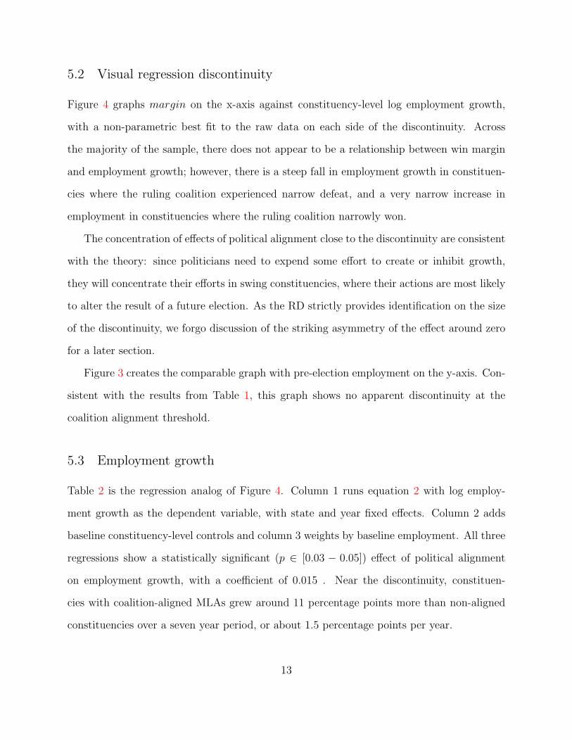
5.2 Visual regression discontinuity
Figure 4 graphs margin on the x-axis against constituency-level log employment growth,
with a non-parametric best fit to the raw data on each side of the discontinuity. Across
the majority of the sample, there does not appear to be a relationship between win margin
and employment growth; however, there is a steep fall in employment growth in constituen-
cies where the ruling coalition experienced narrow defeat, and a very narrow increase in
employment in constituencies where the ruling coalition narrowly won.
The concentration of effects of political alignment close to the discontinuity are consistent
with the theory: since politicians need to expend some effort to create or inhibit growth,
they will concentrate their efforts in swing constituencies, where their actions are most likely
to alter the result of a future election. As the RD strictly provides identification on the size
of the discontinuity, we forgo discussion of the striking asymmetry of the effect around zero
for a later section.
Figure 3 creates the comparable graph with pre-election employment on the y-axis. Con-
sistent with the results from Table 1, this graph shows no apparent discontinuity at the
coalition alignment threshold.
5.3 Employment growth
Table 2 is the regression analog of Figure 4. Column 1 runs equation 2 with log employ-
ment growth as the dependent variable, with state and year fixed effects. Column 2 adds
baseline constituency-level controls and column 3 weights by baseline employment. All three
regressions show a statistically significant (p ∈ [0.03 − 0.05]) effect of political alignment
on employment growth, with a coefficient of 0.015 . Near the discontinuity, constituen-
cies with coalition-aligned MLAs grew around 11 percentage points more than non-aligned
constituencies over a seven year period, or about 1.5 percentage points per year.
13

Columns 4-6 show the result of running equation 3 on the same outcome. The coefficients
are slightly smaller, with the same level of significance.
Figure 5 shows the robustness of these results to alternate kernels and bandwidths. Panel
A shows the treatment effect of equation 2 with bandwidths from 1-10%. Panel B shows the
same information using a rectangular kernel. Panel C repeats limits the election sample to a
4-year window of elections instead of a 5-year window used for Table 2. Panel D shows the
effect of limiting the range of the running variable when running the polynomial specification
in equation 3. The figure demonstrates that the treatment effect is robust to alternate
bandwidth and kernel specifications. Panel D shows that the polynomial estimates are
significantly affected by the inclusion or exclusion of elections won or lost by large margins;
for this reason, we use the more stable local linear regression approach in Equation 2 from
this point forward. Reassuringly, the estimates from Equation 2 fall in the middle of the
range of outcomes produced by the full sample polynomial specification.
5.4 Stock prices
We next consider whether coalition alignment affects the stock prices of publicly traded firms.
If political behavior has known real effects on firm growth, rational market participants
should adjust their valuations of firms as the political environment changes. We measure the
effect of political alignment on firm earnings by conducting an event study (MacKinlay, 1997)
using monthly stock returns from India’s two major stock exchanges.
We matched company headquarters to constituencies using their listed pincodes, and
latitudes and longitudes from the GeoNames pincode database. We focus on companies
located outside of India’s ten largest urban centers, as companies located in major cities are
less likely to do the majority of their business in the constituency where their headquarters are
located. We identified 52 constituencies that experienced 166 close election events between
1990 and 2010, the period for which we have wide stock market coverage.
14

For each event, we calculate cumulative abnormal returns as the residual from a market
model (Equation 4) estimated on a period from 24 months to 6 months prior to an election:
Ri,t = αi + βiRm,t + νi,t (4)
where Rm,t is a value weighted market return index and νi,t is an orthogonal error term.
We estimate Equation 5 to determine whether coalition alignment generates abnormal
returns for local firms in the month following a close election:7
CARi,t−1→t+1 = β0+β1aligni,t+β2margini,t+β3margini,t∗alignedi,t+ζXi,t+ηYt+γSi+εi,t
(5)
The running and forcing variables, margin and aligned are defined as in Equation 2.
CARi,t−1→t+1 is the cumulative abnormal return of a stock from the month before to the
month following an election.8 Xi,t is a vector of constituency controls, and Si and Yt are
state and year fixed effects. β1 identifies the local effect of coalition alignment on stock
returns. As before, we weight with a triangular kernel within the optimal bandwidth.
Table 3 shows the estimation of the event study. Column 1 is the baseline model without
fixed effects. Column 2-4 respectively add fixed effects for (2) state, (3) state and year;
and (4) state * year. Examining the coefficient on aligned, we find that the election of
a coalition-aligned candidate is associated with a positive abnormal return in the range of
12-15% in the month following the election.
Columns 5-6 are placebo tests, using CAR in the month before the election as the depen-
dent variable. If election results are truly a surprise, we should identify no effect of election
outcomes on pre-election returns. As expected, the coefficients are close to zero and not
7Closeness of election in this case is important both for the identification of the RD, and to plausiblybelieve that the anticipated election result has not been priced in before the election takes place.
8We are not able to precisely identify a election outcome date, as voting often takes places on multipledays and results are not officially announced for days or weeks after voting ends. We define the end of ourperiod as the last day of the month in which official electoral results were reported.
15

statistically significant.
These results indicate that the importance of coalition alignment to firm growth is known
and acted upon by market participants. Note that publicly traded firms differ substantially
from the typical firm in the economic census (i.e. the sample for Table 2); finding this result
in both datasets suggests that political behavior affects a wide spectrum of firms.
6 Mechanisms
We next explore the mechanisms that politicians use to affect local employment growth.
We investigate three classes of mechanisms that describe how politicians could substantially
affect employment growth in favored constituencies: (i) pure transfers; (ii) supply of factors
of production; (iii) supply or restriction of regulatory inputs.
6.1 Pure transfers: government jobs and procurement
In this section, we examine transfers from government to firms and individuals.9 We consider
government job creation as a transfer to individuals, and government procurement contracts
as a transfer to firms.
Table 4 separates employment growth in private firms from employment growth in public
firms. In columns 1-3, the dependent variable is employment growth in government-owned
firms, which include all public sector establishments. In columns 4-6, the dependent variable
is employment growth in privately owned establishments. The coefficient of interest is almost
twice as large for private than for government firms, but the difference between the two is
not statistically significant from zero, based on a joint signficance test. The effect of political
favoritism on employment in government firms is not distinguishable from zero, though this
9Our empirical design can only test for differences in transfers between favored and disfavored locations;thus, we cannot tell substitution of transfers from a change in the total level of transfers.
16

is in part due to a larger standard error.10 While we cannot say definitively that the effect
of political favoritism is driven by private sector firms, it is clear that politician influence
over hiring at public sector firms is not driving our main effect.
6.2 Factors of production
In this section, we consider essential inputs to the production function of firms that are
commonly supplied by the state. These include public infrastructure and credit from state-
owned banks.11
The ruling coalition at the state level has control over the location of a substantial share
of local public goods, such as roads, schools, and electricity infrastructure. These government
inputs are essential to operation in many industries, and are too expensive for any but the
largest firms to build at their own expense.
To test the hypothesis that the effect of political favoritism on employment growth is
driven by construction of public infrastructure, we run equation 2 with changes in public
goods between 1991-2001 as dependent variables. Table 5 shows the RD estimates of coalition
alignment on construction of new roads and electricity infrastructure. Columns 1, 2, 4 and
5 use population census data on presence of these public goods; column 3 is based on firm
self-reports of source of power. We can detect no effect on road construction or electricity
connection in towns. The table also reports the mean growth in the dependent variable
over the same period; all our point estimates and standard errors are small relative to mean
growth in this period.
Table 6 shows the effect of coalition alignment on constituency-level growth in schools
and hospitals from 1991 to 2001. None of the coefficients on the alignment variable are sta-
10The larger standard error is in part due to the fact that public employment is only 17-20% of totalemployment over the sample period.
11Credit from state-owned banks could also be considered a transfer; however, given the dominance of thestate in India’s banking sector, formal credit is largely a government-supplied input.
17

tistically distinguishable from zero, and the estimates and standard errors are small relative
to growth in these publicly provided inputs over the sample period.
In summary, there is no indication that the firm-level effect of political favoritism is
being driven by an increase in public infrastructure in favored constituencies. This finding is
consistent with other work on India finding that citizen mobilization and national political
agendas have played the dominant role in determining which regions gained public goods
(Banerjee et al., 2005; Banerjee and Somanathan, 2007).
We next to turn to credit from state owned banks. Lending in India is known to re-
spond to political cycles (Cole, 2009), and data from Brazil suggest that politicians use
state owned banks to reallocate private sector employment growth across legislative con-
stituencies (Carvalho, 2010). To test whether a credit channel can account for the effect
of political favoritism on local employment growth, we run equation ??, adding an interac-
tion term between the electoral variables margin, aligned, margin ∗ aligned, and dummy
variables indicating whether a firms’ dependence on external finance is higher than median.
We draw these measures from two sources: (i) The World Bank Global Enterprise survey
asks firms their share of bank financing over working capital, as well as whether they have
taken new loans this year; (ii) Rajan-Zingales’ industry-level measures of dependence on
external finance dependence (Rajan and Zingales, 1998). In addition to this industry-based
measure of credit demand, we test a location-based measure of credit supply: the presence
of state-owned banks in a constituency, measured as the number of banks per worker.
If credit is the major channel of political influence, these interaction terms should enter
significantly into Equation ??. Table 7 shows the result of these regressions. The first two
columns show industry level measures of credit dependence from the global Enterprise survey:
(1) whether a firm has taken out a new loan in the past year; and (2) bank financing as a
share of working capital. Column 3 repeats column 2 using a measure constructed from the
Indian Annual Survey of Industries. Columns 4 and 5 test whether political favoritism has a
18

larger effect in locations with a large presence of (4) banks; and (5) state-owned banks. None
of the interaction terms are statistically distinguishable from zero, suggesting that neither
demand for credit nor availability of local banks affect the relationship between political
favoritism and economic growth.
6.3 Regulatory inputs
While the Indian Administrative Service is a federal body, state politicians have significant
influence over local bureaucrats, exerted through politicians’ ability to reassign bureaucrats
(Iyer and Mani, 2012). The bureaucracy is an important mechanism for the control of firms
to the extent that firms’ business requires inputs from the government, such as licenses,
permits or land clearances. Using the World Bank Global Enterprise Surveys, we categorize
industries based on the frequency and character of their relationships with public officials.
As above, we create a dummy variable indicating whether an industry has above median
interactions / dependence on government officials, and interact this variable with the RD
variables. If the value of the interaction term is positive, it suggests that political favoritism
has an outsize effect on firms with a high dependence on regulatory inputs.
Table 8 shows the result of the interacted model, with columns 1-4 using the following
measures of dependence on government regulation: (i) Business was visited by government
officials in last year; (ii) Percentage of senior management’s time spent dealing with govern-
ment officials; (iii) Needed an operating license in past year; (iv) Visited by tax officials in
last year. The coefficients on all of four of these interactions are positive and significant,
and the uninteracted measure of coalition alignment is small and indistinguishable from zero.
Political favoritism does not have a large effect on firms that do not require significant inputs
from government bureaucracy. This result is consistent with the idea that politicians exert
political influence through their control of the bureaucracy, and have the ability to make it
easier or more difficult for firms to navigate the regulatory environment.
19

7 Conclusion
Far from competing in an open market on a level playing field, firms in developing countries
often depend heavily on public goods and government inputs. In turn, politicians may also
be significantly affected by firm behavior (Shleifer and Vishny, 1994). This paper draws
on highly localized firm-level employment data to show that politician identity significantly
affects the prospects for firm growth in India.
We show that the alignment of a local politician with the ruling state coalition strongly
predicts increased private sector employment growth in the range of 1 to 2 percentage points
per year. This effect is corroborated by stock prices of large, publicly traded firms: in the
month following elections, firms headquartered in constituencies represented by coalition-
aligned politicians experience a 12-15% cumulative abnormal return.
Examining the most commonly cited mechanisms for political favoritism, we find no
evidence that these effects are driven by geographic preference in government hiring, pro-
curement, or construction of public goods. We do find evidence that the industries most
affected by political favoritism are those with a high dependence on government officials and
government-provided inputs, like licenses and permits, suggesting that politicians are able to
influence the enactment of regulations in geographic areas. This is consistent with evidence
that politicians can exert influence over bureaucrats by threatening geographic reassignment.
The evidence is consistent with a model of rational politicians who take into account the
costs and benefits of the different levers at their disposal. Regulatory discretion is a relatively
low cost tool; in equilibrium, bureaucrats may be pliable even if no transfers take place. India
is well-known for its history of onerous regulations and barriers to the normal operation of
firms. The evidence presented here is consistent with theories that bad regulation can persist
because it gives public officials, in this case politicians, the ability to extract rents from local
firms (Kruger 1974).
20

Table 1Balance Test
Emp Emp (FE) Population Size Count Rural
Aligned (RD) 0.141 0.035 -0.016 0.035 -0.043 -0.041(0.127) (0.101) (0.055) (0.085) (0.144) (0.043)
Margin -5.221 -1.707 -0.593 -2.072 1.754 3.052(3.554) (2.908) (2.437) (2.533) (4.688) (1.585)*
Margin * Aligned 3.566 -1.355 -0.986 -0.876 -2.251 -4.592(4.267) (3.533) (3.428) (3.007) (4.305) (1.846)**
Constant 9.128 8.153 11.266 7.443 2.659 0.891(0.163)*** (0.156)*** (0.106)*** (0.110)*** (0.210)*** (0.064)***
N 663 663 334 663 663 663r2 0.00 0.39 0.72 0.47 0.23 0.32∗p < 0.10,∗∗ p < 0.05,∗∗∗ p < 0.01The table presents kernel regression discontinuity estimates of the effect of politician alignment with state rulingcoalition on constituency level variables measured before the election. The dependent variable in column 1 is logemployment. Column 2 adds state fixed effects. The dependent variables in columns 3-6 are (3) log population;(4) average firm size; (5) number of firms; (6) share of constituency population living in villages. Balance onobservables is robust to inclusion of state and year fixed effects. Standard errors are clustered at the state level.
21

Table 2Effect of MLA alignment on log employment growth
1 2 3 4 5 6
Aligned (RD) 0.016 0.015 0.015 0.011 0.010 0.009(0.008)* (0.007)** (0.007)** (0.005)** (0.005)** (0.005)*
Margin -0.248 -0.239 -0.260 -0.157 -0.150 -0.144(0.234) (0.230) (0.216) (0.049)*** (0.044)*** (0.043)***
Margin * Aligned 0.195 0.117 0.139 0.134 0.134 0.132(0.266) (0.269) (0.252) (0.039)*** (0.050)** (0.047)***
Baseline -0.023 -0.023 -0.018 -0.018(0.005)*** (0.005)*** (0.003)*** (0.003)***
Constant 0.000 0.202 0.197 0.054 0.193 0.194(0.010) (0.044)*** (0.043)*** (0.002)*** (0.027)*** (0.027)***
Weighted No No Yes No No YesControls No Yes Yes No Yes YesN 663 663 663 3625 3625 3625r2 0.13 0.26 0.25 0.09 0.20 0.19∗p < 0.10,∗∗ p < 0.05,∗∗∗ p < 0.01The table shows kernel regression discontinuity estimates of the effect of MLA alignment with state rulingcoalition on change in constituency-level log employment growth from 1990-98 and 1998-2005. Column 1 isthe baseline regression on year and state fixed effects. Column 2 adds constituency-level controls, and column3 weights observations by baseline log employment. Standard errors are clustered at the state level.
22

Table 3Effect of MLA alignment on post-election stock returns
t=0 t=0 t=0 t=0 t=-1 t=-1
Aligned 0.128 0.151 0.121 0.152 -0.014 0.021(0.060)** (0.071)** (0.077) (0.090)* (0.053) (0.081)
Margin -1.699 0.613 1.046 0.693 -0.108 -3.463(1.610) (2.370) (2.839) (3.047) (1.444) (2.750)
Margin * Aligned -2.787 -5.541 -5.431 -6.192 1.968 4.295(3.030) (3.516) (3.922) (4.213) (2.719) (3.803)
Constant -0.004 -0.139 -0.118 -0.086 0.009 -0.191(0.029) (0.127) (0.168) (0.221) (0.026) (0.200)
Fixed Effects None State State,Year State * Year None State * YearN 166 166 166 166 166 166r2 0.03 0.21 0.35 0.36 0.01 0.34∗p < 0.10,∗∗ p < 0.05,∗∗∗ p < 0.01The table shows kernel regression discontinuity estimates of cumulative abnormal returns of publicly tradedfirms in the month following election. The independent variable Aligned indicates the representative of theconstituency where the firm’s headquarters are located is a member of the state ruling coalition. Returns aremeasured against a market model with a value weighted index of Indian securities representing the market.Column 1 is the baseline model without fixed effects. Column 2 adds state and year fixed effects.
23
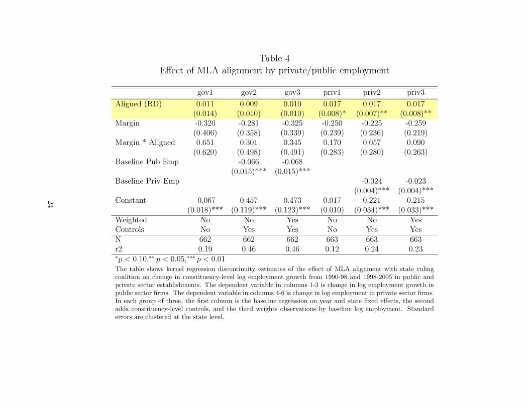
Table 4Effect of MLA alignment by private/public employment
gov1 gov2 gov3 priv1 priv2 priv3
Aligned (RD) 0.011 0.009 0.010 0.017 0.017 0.017(0.014) (0.010) (0.010) (0.008)* (0.007)** (0.008)**
Margin -0.320 -0.281 -0.325 -0.250 -0.225 -0.259(0.406) (0.358) (0.339) (0.239) (0.236) (0.219)
Margin * Aligned 0.651 0.301 0.345 0.170 0.057 0.090(0.620) (0.498) (0.491) (0.283) (0.280) (0.263)
Baseline Pub Emp -0.066 -0.068(0.015)*** (0.015)***
Baseline Priv Emp -0.024 -0.023(0.004)*** (0.004)***
Constant -0.067 0.457 0.473 0.017 0.221 0.215(0.018)*** (0.119)*** (0.123)*** (0.010) (0.034)*** (0.033)***
Weighted No No Yes No No YesControls No Yes Yes No Yes YesN 662 662 662 663 663 663r2 0.19 0.46 0.46 0.12 0.24 0.23∗p < 0.10,∗∗ p < 0.05,∗∗∗ p < 0.01The table shows kernel regression discontinuity estimates of the effect of MLA alignment with state rulingcoalition on change in constituency-level log employment growth from 1990-98 and 1998-2005 in public andprivate sector establishments. The dependent variable in columns 1-3 is change in log employment growth inpublic sector firms. The dependent variable in columns 4-6 is change in log employment in private sector firms.In each group of three, the first column is the baseline regression on year and state fixed effects, the secondadds constituency-level controls, and the third weights observations by baseline log employment. Standarderrors are clustered at the state level.
24

Table 5Effect of MLA alignment on road and electricity growth
Tar Road (r) Tar km (u) Electricity (firm) Electricity (r) Electricity (u)
Aligned (RD) 0.016 0.115 -0.0214 0.043 0.005(0.023) (0.110) (0.0150) (0.031) (0.134)
Margin -1.241 -3.144 2.095 -0.939 3.221(0.559)** (2.996) (3.720) (1.040) (3.621)
Margin * Aligned 1.080 3.617 4.721 1.178 -5.976(0.714) (3.791) (5.322) (1.252) (4.114)
Baseline log population 0.084 0.160 0.081 0.686(0.006)*** (0.044)*** (0.007)*** (0.114)***
Paved approach (village) 0.277(0.016)***
Baseline paved roads (km) -0.006(0.001)***
Mean growth 0.40 0.35 0.09 1.17 0.17N 229 279 610 267 295r2 0.31 0.13 0.15 0.26 0.32∗p < 0.10,∗∗ p < 0.05,∗∗∗ p < 0.01
25

Table 6Effect of MLA alignment on school and hospital growth
Primary Schools Secondary Schools Hospitals
Aligned (RD) -0.022 0.008 -0.023(0.054) (0.049) (0.089)
Margin 0.573 -0.331 3.328(1.337) (1.188) (2.689)
Margin * Aligned 0.779 2.329 -4.083(1.937) (1.720) (3.581)
Baseline log population 0.334 0.285 0.219(0.038)*** (0.028)*** (0.034)***
Mean growth 0.16 0.10 0.12N 325 305 239r2 0.29 0.34 0.22∗p < 0.10,∗∗ p < 0.05,∗∗∗ p < 0.01
The table shows kernel regression discontinuity estimates of the effect of MLA alignmentwith state ruling coalition on change in the levels of local public goods. The dependentvariables in columns 1-3 are all changes in the following variables, from 1991-2001: (1) logprimary schools; (2) log secondary schools; (3) hospitals. All regressions are run at theconstituency level with state and year fixed effects. Standard errors are clustered at thestate level.
26

Table 7Effect of MLA alignment on employment growth, credit supply/demand
interactions
(1) (2) (3) (4) (5)Aligned (RD) 0.113 0.091 0.114 0.163 0.148
(0.053)** (0.066) (0.052)** (0.080)* (0.072)*Aligned * New loans -0.040
(0.045)Aligned * Finance demand (Ent.) 0.048
(0.068)Aligned * Finance demand (ASI) -0.029
(0.111)Aligned * Bank supply -0.111
(0.091)Aligned * Pub bank supply -0.060
(0.104)Constant -0.040 -0.137 -0.013 -0.123 -0.105
(0.076) (0.081) (0.072) (0.083) (0.077)N 1378 1378 1378 689 689r2 0.10 0.16 0.15 0.16 0.16∗p < 0.10,∗∗ p < 0.05,∗∗∗ p < 0.01The table shows kernel regression discontinuity estimates of the effect of MLA alignment with stateruling coalition on change in annualized log employment. The electoral variables relevant to the RD areinteracted with the following measures of industry-level credit demand and location-level credit supply:(i) Demand for new loans (Enterprise survey); (ii) Bank finance / working capital (Enterprise survey);(iii) Dependence on external finance ((Rajan and Zingales, 1998)); (iv) Presence of local banks; (v)Presence of local public sector banks.
27
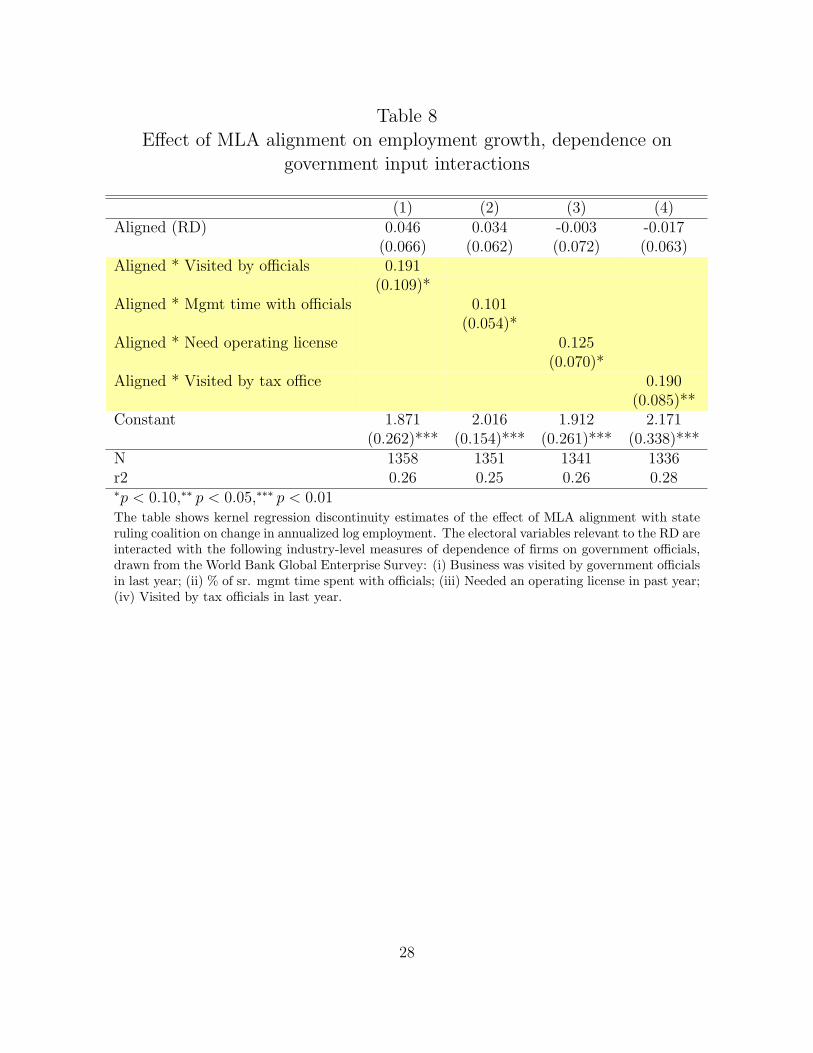
Table 8Effect of MLA alignment on employment growth, dependence on
government input interactions
(1) (2) (3) (4)Aligned (RD) 0.046 0.034 -0.003 -0.017
(0.066) (0.062) (0.072) (0.063)Aligned * Visited by officials 0.191
(0.109)*Aligned * Mgmt time with officials 0.101
(0.054)*Aligned * Need operating license 0.125
(0.070)*Aligned * Visited by tax office 0.190
(0.085)**Constant 1.871 2.016 1.912 2.171
(0.262)*** (0.154)*** (0.261)*** (0.338)***N 1358 1351 1341 1336r2 0.26 0.25 0.26 0.28∗p < 0.10,∗∗ p < 0.05,∗∗∗ p < 0.01The table shows kernel regression discontinuity estimates of the effect of MLA alignment with stateruling coalition on change in annualized log employment. The electoral variables relevant to the RD areinteracted with the following industry-level measures of dependence of firms on government officials,drawn from the World Bank Global Enterprise Survey: (i) Business was visited by government officialsin last year; (ii) % of sr. mgmt time spent with officials; (iii) Needed an operating license in past year;(iv) Visited by tax officials in last year.
28

Figure 1Construction of electoral variables
Election sampleElection sample
Sample election years
Bihar
Assam
Madhya Pradesh
Karnataka
Economic Census
1996 1997 1998 1999 2000 2001 2002 2003 2004 20051990 1991 1992 1993 1994 1995
Growth 1990‐1998Growth 1998‐2005
29
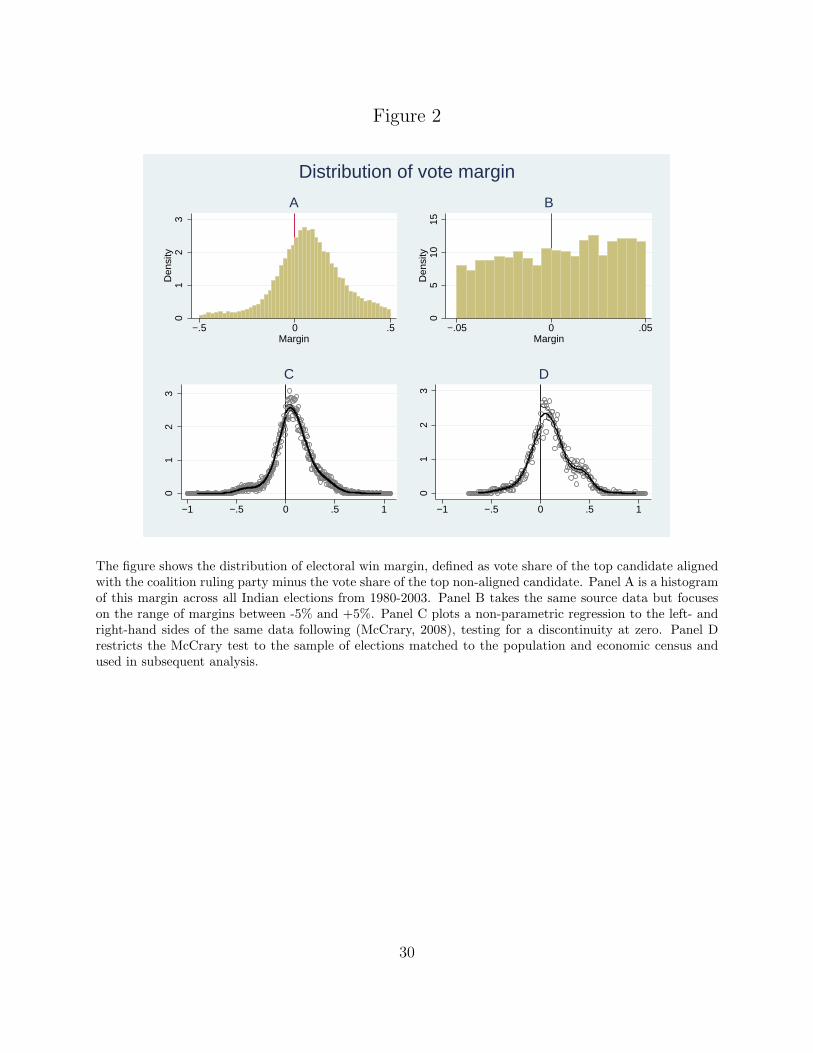
Figure 2
01
23
Den
sity
−.5 0 .5Margin
A
05
1015
Den
sity
−.05 0 .05Margin
B
01
23
−1 −.5 0 .5 1
C
01
23
−1 −.5 0 .5 1
D
Distribution of vote margin
The figure shows the distribution of electoral win margin, defined as vote share of the top candidate alignedwith the coalition ruling party minus the vote share of the top non-aligned candidate. Panel A is a histogramof this margin across all Indian elections from 1980-2003. Panel B takes the same source data but focuseson the range of margins between -5% and +5%. Panel C plots a non-parametric regression to the left- andright-hand sides of the same data following (McCrary, 2008), testing for a discontinuity at zero. Panel Drestricts the McCrary test to the sample of elections matched to the population and economic census andused in subsequent analysis.
30

Figure 3Balance test: Coalition win/loss margin against baseline log employment
88.
59
9.5
10B
asel
ine
log
empl
oym
ent
−.2 0 .2Margin
The figure plots the mean of baseline log employment, in constituencies group by the win margin of thecandidate representing the state ruling coalition. Points to the right of zero are seats won by the rulingcoalition. The bin size represents 0.25 percentage points, and there are approximately six observations ineach bin. A non-parametric smoother is fitted separately to each side of 0.
31
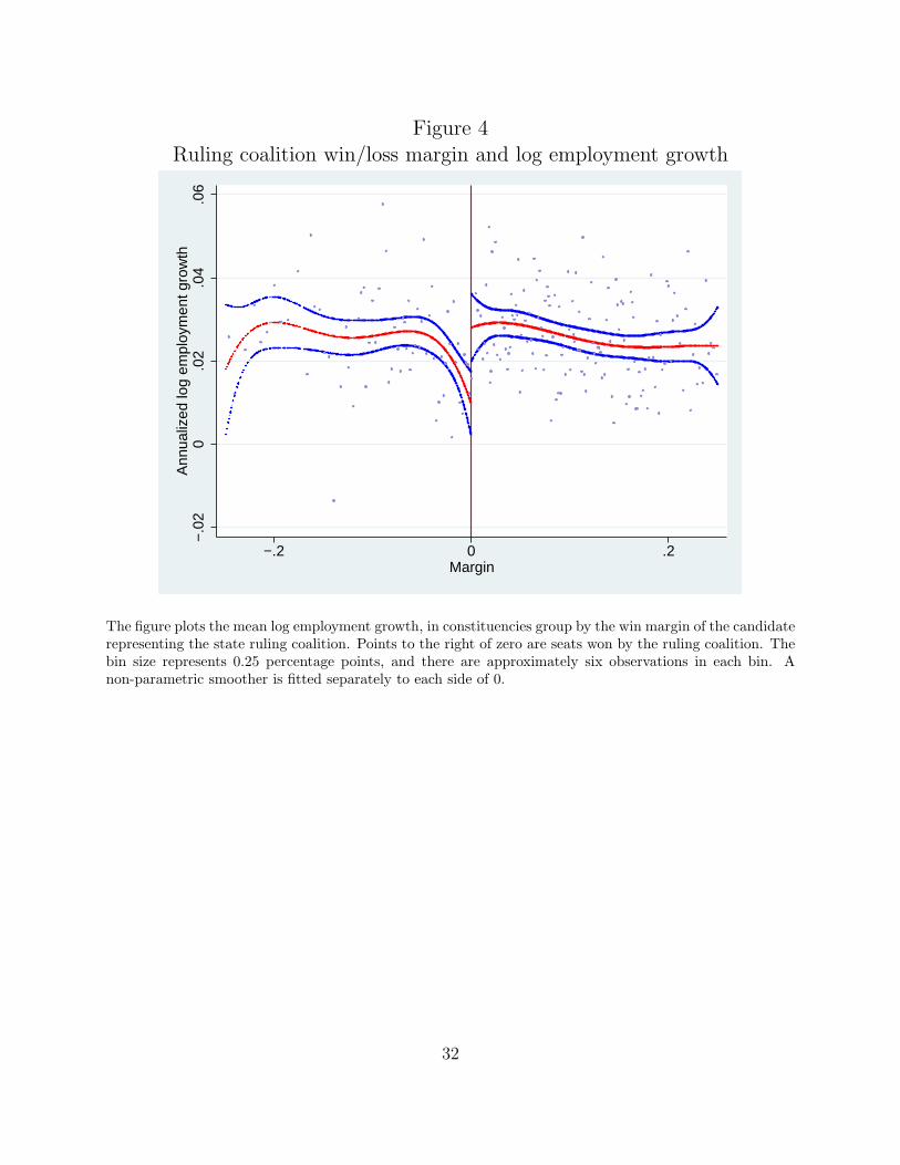
Figure 4Ruling coalition win/loss margin and log employment growth
−.0
20
.02
.04
.06
Ann
ualiz
ed lo
g em
ploy
men
t gro
wth
−.2 0 .2Margin
The figure plots the mean log employment growth, in constituencies group by the win margin of the candidaterepresenting the state ruling coalition. Points to the right of zero are seats won by the ruling coalition. Thebin size represents 0.25 percentage points, and there are approximately six observations in each bin. Anon-parametric smoother is fitted separately to each side of 0.
32

Figure 5Robustness of main effect to alternate specifications
n = 136n = 288
n = 418 n = 545 n = 689 n = 822 n = 983 n = 1131 n = 1253 n = 1372
−.0
10
.01
.02
.03
.04
Log(
grow
th)
0 2 4 6 8 10Bandwidth * 100
A: Triangle kernel
n = 136
n = 288n = 418 n = 545 n = 689
n = 822n = 983 n = 1131 n = 1253 n = 1372
0.0
1.0
2.0
3.0
4.0
5Lo
g(gr
owth
)
0 2 4 6 8 10Bandwidth * 100
B: Rectangular kernel
n = 104
n = 220n = 315
n = 408 n = 514 n = 615 n = 730 n = 835 n = 923 n = 1011
−.0
20
.02
.04
Log(
grow
th)
0 2 4 6 8 10Bandwidth * 100
C: Triangle kernel, 4−year window
n = 1372
n = 2405n = 2959 n = 3265
n = 3501
n = 3593
0.0
1.0
2.0
3.0
4Lo
g(gr
owth
)
10 20 30 40 50 60Range of abs(margin) * 100
Polynomial
This figure plots the point estimate and 90% confidence interval of the constituency-level treatment effectof alignment with governing coalition on annualized log employment growth under a range of specifications.Panel A shows the treatment effect of equation 2 under a range of possible bandwidths. Panel B repeatsPanel A using a rectangular kernel. Panel C repeats Panel A, but using a 4-year window of elections insteadof a 5-year window of elections. Panel D shows the effect of limiting the range of the running variable whenrunning the polynomial specification in equation 3. In each case, the X axis shows in percentage points thevote share of the aligned candidate minus the vote share of the non-aligned candidate.
33

References
Aghion, P, L Boustan, C Hoxby, and J Vandenbussche, “The Causal Impact of Educationon Economic Growth: Evidence from U.S.,” 2009.
Albouy, David, “Partisan Representation in Congress and the Geographic Distribution ofFederal Funds,” 2009.
Ansolabehere, Stephen and James M Snyder, “Party Control of State Government and theDistribution of Public Expenditures,” Scandinavian Journal of Economics, December2006, 108 (4), 547–569.
Arulampalam, Wiji, Sugato Dasgupta, Amrita Dhillon, and Bhaskar Dutta, “Electoral goalsand center-state transfers: A theoretical model and empirical evidence from India,”Journal of Development Economics, January 2009, 88 (1), 103–119.
Banerjee, Abhijit and Rohini Somanathan, “The political economy of public goods: Someevidence from India,” Journal of Development Economics, March 2007, 82 (2), 287–314.
, Lakshmi Iyer, and Rohini Somanathan, “History, Social Divisions, and Public Goodsin Rural India,” Journal of the European Economic Association, 2005, 3 (2), 639–647.
Brollo, Fernanda and Tommaso Nannicini, “Tying Your Enemy’s Hands in Close Races: ThePolitics of Federal Transfers in Brazil,” 2011.
Carvalho, D R, “The Real Effects of Government-Owned Banks: Evidence from an EmergingMarket,” 2010.
Chattopadhyay, R and E Duflo, “Women as Policy Makers : Evidence from a RandomizedPolicy Experiment in India,” Econometrica, 2004, 72 (5), 1409–1443.
Chhibber, Pradeep, Sandeep Shastri, and Richard Sisson, “Federal Arrangements and theProvision of Public Goods in India,” Asian Survey, June 2004, 44 (3), 339–352.
Cohen, Lauren, Joshua Coval, and Christopher Malloy, “Do Powerful Politicians CauseCorporate Downsizing,” Journal of Political Economy, 2011, 119 (6), 1015–1060.
Cole, Shawn, “Fixing Market Failures or Fixing Elections? Agricultural Credit in India,”American Economic Journal: Applied Economics, January 2009, 1 (1), 219–250.
, Andrew Healy, and Eric Werker, “Do voters demand responsive governments? Evi-dence from Indian disaster relief,” Journal of Development Economics, March 2012, 97(2), 167–181.
de Janvry, Alain, Frederico Finan, and Elisabeth Sadoulet, “Local Electoral Incentives andDecentralized Program Performance,” 2010.
34

Dixit, Avinash and John Londregan, “The Determinants of Success of Special Interests inRedistributive Politics,” The Journal of Politics, 1996, 58 (4), 1132–1155.
Finan, Frederico S, “Political Patronage and Local Development : A Brazilian Case Study,”2004, (April).
Hoover, Gary A and Paul Pecorino, “The Political Determinants of Federal Expenditure atthe State Level,” Public Choice, 2005, 123, 95–113.
Iyer, Lakshmi and Anandi Mani, “Traveling Agents: Political Change and BureaucraticTurnover in India,” The Review of Economics and Statistics, 2012, 94 (3), 723–739.
Khemani, S., “Does delegation of fiscal policy to an independent agency make a differ-ence? Evidence from intergovernmental transfers in India,” Journal of DevelopmentEconomics, 2007, 82 (2), 464–484.
Lindbeck, Assar and Jorgen Weibull, “A model of political equilibrium representative democ-racy,” Journal of Public Economic Theory, 1993, 51 (June 1990), 195–209.
MacKinlay, A Craig, “Event Studies in Economics and Finance,” Journal of Economic Lit-erature, 1997, 35 (1), 13–39.
McCrary, Justin, “Manipulation of the running variable in the regression discontinuity de-sign: A density test,” Journal of Econometrics, February 2008, 142 (2), 698–714.
Rajan, Raghuram and Luigi Zingales, “Financial Dependence and Growth,” The AmericanEconomic Review, February 1998, 88 (3), 559–586.
Shleifer, Andrei and Robert W. Vishny, “Politicians and Firms,” Quarterly Journal of Eco-nomics, 1994, 109 (4), 995–1025.
Shoag, Daniel, “The Impact of Government Spending Shocks: Evidence on the Multiplierfrom State Pension Plan Returns,” 2011.
Sukhtankar, Sandip, “Sweetening the Deal? Political Connections and Sugar Mills in India,”2012.
Wolfers, Justin, “Are Voters Rational ? Evidence from Gubernatorial Elections,” 2007.
35