political fragmentation and fiscal policy - ntanet.org · political fragmentation and fiscal policy...

Political Fragmentation and Fiscal Policy

Enda Patrick Hargaden∗

Department of Economics

University of Michigan

[email protected]

Version of November 4, 2014

Abstract

This paper examines the link between political fragmentation and tax policy. A model ofgovernment is presented where an n-member coalition chooses revenue and expenditure policies.I derive the response of tax policy to a change in the number of coalition partners. The modelpredicts that an increase in the number of parties leads to (i) lower taxes; (ii) lower expenditure;and (iii) lower social security transfers. These results are counter to the conventional wisdomthat countries with more fragmented governments have larger public sectors. I test the model ona large panel of developed countries, and all three of the model’s predictions are supported. Myresults have coefficients significantly different from, and of opposing signs to, the conventionalwisdom. I estimate that moving from a two- to three-party legislature lowers tax revenueby 6.7%, expenditure by 9.5%, and transfers by 5.4%. These results are robust to a host ofpotentially important variables such as the ideological composition of government, changes inthe tax base, and electoral cycle effects.

∗I would like to thank David Albouy, Eric Chyn, Jason Kerwin, Ben Meiselman, Joel Slemrod; participants atthe University of Michigan’s Public Economics summer talks seminar, the Michigan Tax Invitational conference, theBarcelona GSE Political Economy summer school; and particularly Jim Hines and Ugo Troiano for their commentsand advice on this paper.

1

1 Introduction

The paper investigates how legislative fragmentation affects the size of government. The conventional

wisdom (cf. Weingast et al. (1981) Lijphart (1984), Austen-Smith (2000), Milesi-Ferretti et al. (2002))

is that a larger number of political parties leads to an increase in a country’s taxes, spending, and

transfers.

This paper makes both theoretical and empirical contributions that challenge the conventional

wisdom. I model the government’s choice of tax rates, public good provision, and level of transfers as a

function of n coalition partners. Unlike many models that assume an exogenous revenue requirement,

the model allows government income and expenditure to be endogenous. The model predicts that an

increase in coalition size leads to lower taxes, spending, and transfers. All three of these predictions

are supported in data from a large panel of OECD countries. I estimate that moving from a two-

to three-party legislature lowers tax revenue by 6.7%, expenditure by 9.5%, and transfers by 5.4%

I first replicate the relationship predicted by the conventional wisdom by excluding country fixed

effects. Including fixed effects completely changes the results. Rather than a positive relationship, I

find negative and statistically significant coefficients. These results are robust to a host of potentially

important variables such as the ideological composition of government, changes in the tax base, and

electoral cycle effects.

In 2008 the share of the United States’ total government expenditure over GDP was 37% while

the average for EU countries was 47%. Electoral incentives facing governments can help explain

this variation. The correspondence between politics and taxes is crucial in determining society’s

preferred size of government. This paper investigates the effect of increased legislative fragmentation

(as measured by the seats-weighted number of parties in parliament) on tax policy, and thus the

paper contributes to understanding the effects of secular fragmentation. Additionally, the paper has

implications for policies to increase the number of political parties, such as the 2011 electoral reform

referendum in the UK.

Research on the link between political science and tax policy, and the debate about the ‘varieties

of capitalism’ (Hall and Soskice, 2001), is not new. The empirical work of Lijphart (1984, 1999)

2

showed statistically significant relationships between the number of political parties and tax policies.

Lijphart concluded that fragmentation leads to broad, consensus-based coalitions which cause gov-

ernments to become “kindler, gentler”. Although investigating the distinct question about the link

between tax policy and electoral systems, Milesi-Ferretti, Perotti and Rostagno (2002) show that the

proportionality of electoral systems increases public spending and transfers, and that these results

hold even within the subset of proportional representative (PR) systems. Kontopoulos and Perotti

(1999) were confident enough that fragmentation increased expenditure to perform a one-sided test

on their coefficient of interest.

Theoretical models have drawn similar conclusions. The ‘veto player’ model (Tsebelis, 2002)

focuses on the ability of a coalition of n ≥ 1 ‘veto players’ to change a policy. The intersection of sets

of desirable policies is defined as the ‘winset’ for this coalition. It is straight-forward to understand

the logic that the winset is decreasing in n. One way to ‘grease the wheels’ is by increasing the payoffs

to veto players, which requires higher taxes in equilibrium. Therefore this alternative framework

draws the same conclusion as the conventional wisdom: increasing the number of parties makes

agreement more difficult, and thus higher side-payments (political pork) are necessary.

The empirical analysis of this paper contradicts this view. Pettersson-Lidbom (2012) finds similar

results from two quasi-experiments in Finland and Sweden. This paper is the first to reach similar

conclusions both theoretically and with a dataset on a large number of developed countries. Although

the empirical section may not be as cleanly identified as a small quasi-experimental setting, the

inclusion of many countries in the analysis reduces concerns about external validity.

2 Theoretical Model

The research question of this paper is how a change in the size of an n-member coalition affects tax

policy. More generally, I ask how the collective outcomes for a group are affected by the size of that

group. This setting is well-suited to analysis as a common pool problem.

Most public finance common pool models are driven by the disconnect of taxing power and

spending power, cf. Persson and Tabellini (2002). In these models, decentralized units choose

3

expenditure levels and the central government raises taxes to meet the liabilities that fall due.

Each decentralized unit, knowing that they will only have to pay a fraction of an additional dollar

of expenditure, increases spending.

This approach is equivalent to the usual public finance assumption of governments having to

raise an exogenous amount of revenue. This assumption rules out the possibility of e.g. governments

increasing taxes if spending suddenly becomes more desirable.

I will model the coalition’s choice of policy as a common pool problem. However the coalition will

simultaneously choose income and expenditure policies, and therefore trade off the marginal benefits

and marginal costs of taxation. In this framework taxes and expenditure become endogenous.

There are two types of public good, G1 and G2. The first are the traditional pure public good

that benefits all of society, e.g. national defence, weather forecasts. The second are “local public

goods” which are to the benefit of one large group rather than the general public, e.g. agricultural

subsidies, social security transfers. A simpler version of the model with a single type of public good,

and where taxes are determined residually, can be found in Chapter 7 of Persson and Tabellini

(2002).

A government consists of i = 1, . . . , n political groups. Politician i in government optimizes group

i’s welfare. This is the sum of the group’s after tax income (1 − τ)Yi, an increasing and concave

function f of the pure public good G1, and an increasing and concave function g of group i’s local

public good G2. For convenience I assume that all n parties split G2 equally, but I suspect that the

results hold for more general decreasing functions of n. Formally, given a national income M , the

politician optimizes the following problem:

maxG1,G2,τ

(1− τ)Yi + f (G1) + g

(G2

n

)s.t. G1 +G2 ≤ τM

This is a tractable formulation that departs from much of the previous literature on policy formation.

For instance, the Weingast, Shepsle and Johnsen (1981) ‘Law of 1/n’ assumes a norm of reciprocity in

US Congress, which “facilitates a process of mutual support and logrolling”. This increases inefficient

4

spending in the n number of represented districts. In contrast, I make no such assumption. Rather,

this formulation is intuitively very simple: it is a welfare maximization problem. An n-member

coalition is formed, this coalition commands a majority, and they agree to maximize the welfare of

the groups that comprise the coalition. The assumption of particular norms can of course facilitate

alternative equilibrium outcomes. Within the group, no solution can Pareto dominate the outcome

offered by this formulation.

Assuming the budget constraint holds with equality, any two choice variables will determine the

third. Therefore I define α as the fraction of tax revenue devoted to G2, and in so doing we can

condense the problem into a single maximand in two variables (α and τ) and three parameters (Yi,

M , and n):

maxα,τ

Π = (1− τ)Yi + f ((1− α)τM) + g

(ατM

n

)

This leads to the following first-order conditions:

∂Π

∂α: −τMf ′ ((1− α)τM) +

τM

ng′(ατM

n

)= 0 (F1)

∂Π

∂τ: −Yi + (1− α)Mf ′ ((1− α)τM) +

αM

ng′(ατM

n

)= 0 (F2)

and the following set of second-order and cross-partial derivatives:

∂F1

∂α=(τM)2f ′′ ((1− α)τM) +

(τM

n

)2

g′′(ατM

n

)< 0

=(τM)2[f ′′ ((1− α)τM) +

(1

n2

)g′′(ατM

n

)]< 0 (1)

∂F1

∂τ=−M [f ′ ((1− α)τM) + (1− α)τMf ′′ ((1− α)τM)]

+M

n

[g′(ατM

n

)+ατM

ng′′(ατM

n

)](2)

∂F2

∂α=∂F1

∂τ

∂F2

∂τ= ((1− α)M)

2f ′′ ((1− α)τM) +

(αM

n

)2

g′′(ατM

n

)< 0 (3)

5

The comparative statics addressing how policy responds to fragmentation will also require

differentiating the first-order conditions (F1) and (F2) with respect to n:

∂F1

∂n= −

(τM

n2

)(g′(ατM

n

)+ατM

ng′′(ατM

n

))(4)

∂F2

∂n= −

(αM

n2

)(g′(ατM

n

)+ατM

ng′′(ατM

n

))(5)

It is instructive at this point to note an assumption of the model. Suppose for now that α were

pre-determined and the government’s only choice variable were τ . We can see how n affects taxes

by computing the sign of∂2Π

∂τ∂n, i.e. computing the sign of Equation (5). Clearly −αMn2 is negative.

As g is concave, its first derivative is positive and its second is negative. The sign of the overall

derivative thus depends on the sign of g′(ατMn

)+ ατM

n g′′(ατMn

).

There is some ambiguity on this condition. My results require that the sign here is strictly

positive. Note that this requirement, that g′ (x) + xg′′ (x) > 0, is true for a broad class of concave

functions, such as g(x) = xβ where β < 0. To proceed, I assume that g′ (x) + xg′′ (x) > 0. Under

this assumption we may conclude that Equation (5) is negative: an increase in n will lower taxes.

Similar conclusions can be drawn about α from Equation (4).

Comparative statics are of course more complex for the multivariate optimization problem. This

requires us to account for cross-partial effects of τ on α, etc. Firstly, given that both of the first-order

conditions (F1) and (F2) will equal zero in equilibrium, we can use the Chain Rule to note that:

∂F1

∂α

∂F1

∂τ∂F2

∂α

∂F2

∂τ

∂α

∂n∂τ

∂n

= −

∂F1

∂n∂F2

∂n

(6)

With these derivatives, we have a system of equations that implicitly define how our variables

6

of interest are affected by n:

∂α

∂n∂τ

∂n

= −

∂F1

∂α

∂F1

∂τ∂F2

∂α

∂F2

∂τ

−1

∂F1

∂n∂F2

∂n

(7)

Our first key comparative static is∂α

∂n, how the proportion of resources for the targeted local

public good respond to a change in fragmentation. A positive coefficient here indicates that more

‘pork’ occurs with more parties. We can calculate the sign of this derivative by applying Cramer’s

Rule to Equation (7):

(8)∂α

∂n= −

∂F1

∂n

∂F2

∂τ− ∂F1

∂τ

∂F2

∂n∂F1

∂α

∂F2

∂τ− ∂F1

∂τ

∂F2

∂α

The numerator of this comparative static is

(∂F1

∂n

∂F2

∂τ

)−(∂F1

∂τ

∂F2

∂n

). For the first two terms,

we know that

∂F1

∂n= −

(τM

n2

)(g′(ατM

n

)+ατM

ng′′(ατM

n

))(9)

∂F2

∂τ= ((1− α)M)

2f ′′ ((1− α)τM) +

(αM

n

)2

g′′(ατM

n

)= (M)

2

[(1− α)2f ′′ ((1− α)τM) +

(αn

)2g′′(ατM

n

)](10)

Therefore the product∂F1

∂n

∂F2

∂τequals

−(τM3

n2

) [(1− α)2f ′′ ((1− α)τM) +

(αn

)2g′′(ατMn

)] [g′(ατMn

)+ ατM

n g′′(ατMn

)](11)

7

For the latter two terms in the numerator,∂F1

∂τand

∂F2

∂n, we know that

∂F1

∂τ=−M [f ′ ((1− α)τM) + (1− α)τMf ′′ ((1− α)τM)]

+M

n

[g′(ατM

n

)+ατM

ng′′(ατM

n

)](12)

but from (F1) it is clear that f ′ ((1− α)τM) =(1n

)g′(ατMn

). Substituting this into Equation (12),

it follows that

∂F1

∂τ=−M

[(1

n

)g′(ατM

n

)+ (1− α)τMf ′′ ((1− α)τM)

]+M

n

[g′(ατM

n

)+ατM

ng′′(ατM

n

)](13)

=−M [(1− α)τMf ′′ ((1− α)τM)] +M

n

[ατM

ng′′(ατM

n

)](14)

and therefore

∂F1

∂τ= (−τM2)

{(1− α)f ′′ ((1− α)τM)−

(1

n

)2

αg′′(ατM

n

)}(15)

Finally,

∂F2

∂n= −

(αM

n2

)(g′(ατM

n

)+ατM

ng′′(ατM

n

))(16)

Combining these two together, and temporarily omitting arguments of functions for clarity, we get

∂F1

∂τ

∂F2

∂n=(τM3

n2

)(α)

[(1− α)f ′′ (.) + α

(1n

)2g′′ (.)

] [g′ (.) + ατM

n g′′ (.)]

(17)

8

Formulating the full numerator as the difference between Equation (11) and Equation (17)

∂F1

∂n

∂F2

∂τ− ∂F1

∂τ

∂F2

∂n= −

(τM3

n2

) [(1− α)2f ′′ (.) +

(αn

)2g′′ (.) + α(1− α)f ′′ (.) +

(αn

)2g′′ (.)

](18)

= −(τM3

n2

)︸︷︷︸

<0

(1− α)f ′′ (.)︸︷︷︸<0

+ 2(αn

)2g′′ (.)︸︷︷︸

<0

(19)

> 0 (20)

The denominator of this comparative static is also the difference of two products. In terms of

the first product, we know that

∂F1

∂α= (tM)

2

[f ′′ ((1− α)τM) +

(1

n2

)g′′(ατM

n

)](21)

∂F2

∂τ= (M)

2

[(1− α)2f ′′ ((1− α)τM) +

(αn

)2g′′(ατM

n

)](22)

Omitting the arguments of functions for clarity, we conclude that

∂F1

∂α

∂F2

∂τ= (τ2M4)

{(1− α)2 [f ′′ (.)]

2+(1n

)2 (α2 + (1− α)2

)[f ′′ (.)] [g′′ (.)] + α2

(1n

)4[g′′ (.)]

}(23)

In terms of the second product in the denominator, we have already seen from Equation (2) that

∂F1

∂τ= (−τM2)

{(1− α)f ′′ ((1− α)τM)−

(1

n

)2

αg′′(ατM

n

)}(24)

Because∂F1

∂τ=

∂F2

∂αit follows that

∂F1

∂τ

∂F2

∂α=

(∂F1

∂τ

)2

. Again omitting the arguments of

functions for clarity, we conclude that

∂F1

∂τ

∂F2

∂α= (τ2M4)

{(1− α)2 [f ′′ (.)]

2 − 2α(1− α)(1n

)2[f ′′ (.)] [g′′ (.)] +

(1n

)4α2 [g′′ (.)]

2}

(25)

9

The denominator is equal to Equation (23) less Equation (25). This equals:

∂F1

∂α

∂F2

∂τ− ∂F1

∂τ

∂F2

∂α=

(τ2M4

n2

)︸︷︷︸

>0

[f ′′ ((1− α)τM)]︸︷︷︸<0

[g′′(ατM

n

)]︸︷︷︸

<0

(26)

Putting this all together we find that

∂α

∂n= −

−(τM3

n2

)︸︷︷︸

<0

(1− α)︸︷︷︸>0

f ′′ ((1− α)τM)︸︷︷︸<0

+ 2(αn

)2︸︷︷︸

>0

g′′(ατM

n

)︸︷︷︸

<0

(τ2M4

n2

)︸︷︷︸

>0

[f ′′ ((1− α)τM)]︸︷︷︸<0

[g′′(ατM

n

)]︸︷︷︸

<0

(27)

=(1− α)f ′′ ((1− α)τM) + 2

(αn

)2g′′(ατMn

)(τM) (f ′′ ((1− α)τM))

(g′′(ατMn

)) (28)

∴∂α

∂n< 0

As suggested by the univariate example, this coefficient is negative. Both numerator and denominator

are positive, and the negative sign before the fraction ensures a negative relationship.

The next key comparative static is∂τ

∂n, how the tax rate responds to a change in fragmentation.

A positive coefficient indicates that taxes go up when the number of parties increases.

∂τ

∂n= −

∂F1

∂α

∂F2

∂n− ∂F1

∂n

∂F2

∂α∂F1

∂α

∂F2

∂τ− ∂F1

∂τ

∂F2

∂α

(29)

Note that the denominator here is the same as derived above, which simplifies the computation.

The numerator also contains terms that we have simplified. From Equation (1) we know that

∂F1

∂α= (τM)2

[f ′′ ((1− α)τM) +

(1

n2

)g′′(ατM

n

)](30)

10

From Equation (5) we know that

∂F2

∂n= −

(αM

n2

)(g′(ατM

n

)+ατM

ng′′(ατM

n

))(31)

Therefore their product equals

∂F1

∂α

∂F2

∂n= −

(ατ2M3

n2

)[f ′′ (.) +

(1

n

)2

g′′ (.)

] [g′ (.) +

ατM

ng′′ (.)

](32)


∂F1

∂n= −

(τM

n2

)(g′(ατM

n

)+ατM

ng′′(ατM

n

))(33)


∂F2

∂α=∂F1

∂τ= (−τM2)

{(1− α)f ′′ ((1− α)τM)−

(1

n

)2

αg′′(ατM

n

)}(34)

Therefore their product equals.

∂F1

∂n

∂F2

∂α=

(τ2M3

n2

)[(1− α)f ′′ (.)− α

(1

n

)2

g′′ (.)

] [g′ (.) +

ατM

ng′′ (.)

](35)

The numerator of∂τ

∂nis thus equal to Equation (32) minus Equation (35). When including the

denominator from Equation (26), we get the following result:

∂τ

∂n= −

− f ′′ ((1− α)τM)︸︷︷︸<0

− 2α

(1

n

)2

︸︷︷︸>0

g′′(ατM

n

)︸︷︷︸

<0(τ2M4

n2

)︸︷︷︸

>0

[f ′′ ((1− α)τM)]︸︷︷︸<0

[g′′(ατM

n

)]︸︷︷︸

<0

(36)

∴∂τ

∂n< 0

11

2.1 Summary of Implications

The model presented is an n-member common pool problem. The coalition simultaneously choose

the tax rate τ , and the fraction α of tax revenue directed to local public goods/transfers. The

analysis predicted that taxes fall when n increases. This implies that spending falls when n increases.

The comparative statics also predicted that α falls when n increases. These are the main predictions

of the model. I test these predictions in Section 3.2.

The theory provides a stronger testable implication than those listed above. It is clear that both

transfers and spending should decrease as n increases. However α is defined as transfers as a fraction

of government revenue, not just transfers as a fraction of GDP. I refer to α as “transfer intensity”.

The model predicts that α, transfer intensity, should fall as n increases.

A further implication of the model is nonlinearity in the marginal effects. As both τ and α are

fractions bounded by [0, 1] we do not expect a constant effect of a change in n. In particular, a

marginal change in n at low levels (e.g. from two to three parties) is expected to have a larger effect

than a change at high levels (e.g. from six to seven parties). I test this prediction in Section 3.9.

12

3 Empirical Analysis

3.1 Data Description

The data (Armingeon et al., 2012b) are from the Institute of Political Science at the University of

Bern. This includes measures of political competition as well as primary macroeconomic variables

such as government revenue and social security transfers for 23 countries1 from 1975–2010.2 We see

that nations with more parties have larger government sectors.

Australia

Austria Belgium

Canada

Denmark

FinlandFrance

Germany

Greece Iceland

Ireland

Italy

Japan

Luxembourg

Netherlands

New Zealand

Norway

PortugalSpain

Sweden

Switzerland

UK

USA

3540

4550

5560

Gov

ernm

ent E

xpen

ditu

re (

% G

DP

)

2 4 6 8Parties in Parliament (average)

Average Spending and Number of Parties

Figure 1: The conventional wisdom on spending

Measuring the number of political parties in a country is a non-trivial exercise. Although there

1Australia, Austria, Belgium, Canada, Denmark, Finland, France, Germany, Greece, Iceland, Ireland, Italy, Japan,Luxembourg, Netherlands, New Zealand, Norway, Portugal, Spain, Sweden, Switzerland, UK, and USA.

2The data extend back to 1960 but are less reliable pre-1975. For example, in some specifications I include nationaldebt as a control variable. Prior to 1975, more than half (60%) of values for debt are missing, whereas 8% are missingfor post-1975. For legislative fragmentation, 11% of the values are missing for the period before 1975, and 0.1% aremissing for the period after.

13

are over 400 parties registered in the United Kingdom, three dominate parliament. Similarly, the

United States is considered a two-party system, despite the existence of Libertarians, Greens, etc. To

accounts for this, Lijphart (1984) uses the ‘effective number of parties’, taking weighted averages of

parties’ importance in elections and parliament. The computation is comparable to the Herfindahl

concentration index. In a legislature with m parties, and where si denotes the vote share for party i,

Effective number of parties in parliament =

(m∑i=1

s2i

)−1

The median value of this measure of legislative fragmentation is 3.2 and the standard deviation is

1.4. The US has particularly low values: over the period 1975–2010 the mean is 1.95 with a standard

deviation of 0.06.

Table 1: Summary statistics for 23 countries, 1975–2010

Mean Std. Dev N Min Max

Gov’t receipts (% GDP) 42.56 8.40 785 24.35 63.20

Gov’t expenditure (% GDP) 45.14 8.18 785 26.07 70.54

Gov’t transfers (% GDP) 13.68 3.88 820 4.34 23.89

Eff. parties parliament 3.59 1.43 826 1.69 9.07

Transfers (% Gov’t receipts) 31.94 7.33 783 11.89 55.41

Unemployment benefits (% Gov’t receipts) 3.06 2.15 636 0.00 11.56

Old age benefits (% Gov’t receipts) 16.28 6.01 639 4.82 35.42

Active labor market programs (% Gov’t receipts) 1.54 0.89 566 0.00 4.72

Recall that the main predictions of the model were that taxes, spending, and transfers fall as

the number of coalition partners rise. For the purposes of the empirical analysis, my measures are

total tax receipts as a percent of GDP, total outlays of government as a percent of GDP, and social

security transfers as a percent of GDP. Summary statistics are provided in Table 1.

In addition, the theory makes a sharper prediction: that transfers as a fraction of government

revenue falls when fragmentation increases. This fraction, labeled α, has several empirical analogs.

The data permit testing this prediction with four variants of economic transfers: all social security

14

transfers, unemployment benefits, old age benefits, and expenditure on active labor market programs.

Unemployment benefits and active labor market programs are clearly expenditure targeted at specific

groups more vulnerable to labor market fluctuations; and old age benefits are not pure public goods.

I primarily measure political competition by the effective number of parties in parliament.

Therefore the empirical results in Section 3.2 measure the impact of legislative fragmentation on

tax policy. I find that legislative fragmentation is indeed correlated with tax policy. As we will soon

see, I find that its impact is of the opposing sign and is statistically different from the conventional

approach.

Legislative fragmentation, of course, is distinct from executive/government fragmentation. For

example, fragmentation that is restricted exclusively to opposition parties may not correspond

to increased executive fragmentation. Some previous work (cf. Kontopoulos and Perotti (1999))

emphasize the importance of this distinction. Therefore in Section 3.3 I will largely repeat the

analysis of legislative fragmentation but instead use measures of executive fragmentation.

3.2 Legislative Fragmentation

The empirical analysis is based on a country fixed effect model:

yit = ai + δt + βxit + εit

where yit is the outcome (e.g. tax receipts as a fraction of GDP) in country i during year t; the ai

variables are country fixed effects; δt represents year fixed effects; xit are country-year covariates

(such as legislative fragmentation); and εit is the error term. The standard condition for parameter

identification,

E [εit|xit, ai, δt] = 0

holds when the change in level of fragmentation is exogenous conditional on fixed effects.

The fixed effects model exploits within country variation, rather than between country variation,

to derive results. The estimation is thus based on changes in the number of parties within a country.

This approach captures all time-invariant, country-specific heterogeneity, and isolates that effect

15

from any (time-invariant) spurious relationships between countries’ number of parties and public

finances. Estimation with country fixed effects therefore entirely nests many other approaches, e.g.

the ethnolinguistic fractionalization data explored in Alesina et al. (2003).

Identification is not compromised by disgruntled electorates changing party allegiances, e.g.

switching from Democrats to Republicans. Identification requires that, conditional on observable

characteristics, fragmentation is exogenous. This is a much more reasonable claim.

Of course any time-varying heterogeneity could also bias the estimator. This is less likely to be a

problem with shorter time-horizons and wider cross-sections. For this reason, I repeat the procedure

on a wider sample of 35 countries, including those previously behind the Iron Curtain, which is

available for the year 1990–2010. These results are in Section 3.4.

Table 2 presents the main empirical contribution of the paper. It shows the results, with and

without country fixed effects, of regressing tax policy on legislative fragmentation. Standard errors

are robust to heteroskedasticity and serial correlation, are consistent even under cross-sectional

dependence (Driscoll and Kraay, 1998), and I use the standard lag length as suggested by Newey

and West (1994).

Table 2: Decline in taxes, spending, and transfers

Receipts Expenditure Transfers

(1) (2) (3) (4) (5) (6)

Eff. parties parliament 2.309∗∗∗ -1.045∗∗∗ 1.894∗∗∗ -1.939∗∗∗ 0.615∗∗∗ -0.697∗∗∗

(0.198) (0.319) (0.178) (0.430) (0.0816) (0.156)

Year FE Yes Yes Yes Yes Yes Yes

Country FE No Yes No Yes No Yes

N 783 783 783 783 818 818

Driscoll-Kraay standard errors in parentheses

∗ p < 0.10, ∗∗ p < 0.05, ∗∗∗ p < 0.01

Let us first look at the results on tax revenue presented in Columns 1 and 2. Column 1 presents the

‘conventional wisdom’ estimates, based on between-country regressions. My preferred specification,

including country fixed effects, is shown in Column 2.

16

The first column presents evidence supporting Lijphart (1984)’s conclusion that more parties

leads to higher tax receipts. These results are positive and significant at the 1% level. Column 1

suggests that if the UK moved from a three- to a four-party system, the fraction of output collected

by the government would increase by about 2.3 percentage points.

Column 2, which has the potential to nest Column 1 but isolates any arbitrary country hetero-

geneity, shows a negative coefficient. This suggests that moving from a three- to four-party system

would lower tax revenue by about a percentage point. This result is also highly significant. Crucially,

however, it is a different sign. The approach in Column 2, which is preferable to that employed

in Column 1, reaches an opposite conclusion. As predicted by the group maximization problem in

Section 2, increased legislative fragmentation is associated with lower tax receipts.

Next we look at government expenditure. The columns have the same interpretation as before.

Our coefficients again change sign: Column 3 suggests increasing the number of parties by one

will increase government expenditure by about 2 percentage points; Column 4 suggests it would

decrease expenditure by a similar amount. Again, the results are of opposing sign, and counter to the

conventional wisdom. As predicted by the model, we find lower spending with more fragmentation.

What of transfers? Recall the model in Section 2. Defining α as the share of government revenue

going to transfers to certain groups, we found∂α

∂n< 0, i.e. transfers will fall as the number of parties

increase. This implies that transfers must fall when fragmentation rises.

The pattern emerges again. The between country estimator finds a positive effect, the within

country estimator a negative effect, and the difference is significant. The between estimate suggests

an increase in fragmentation leads to a 0.6 percentage point increase in social security transfers. The

within estimate suggests the same increase in fragmentation would reduce social security transfers

by 0.7 percentage points.

In truth the model makes a stronger prediction. Not just is it predicted that transfers fall but that

transfers as a fraction of government revenue falls. I call this “transfer intensity”. The prediction

that transfer intensity falls is tested in Table 3. This time, both between and within estimates

suggest a negative sign. Again, the prediction is validated by the fixed effects estimates, and the

result is significant at the 1% confidence level.

17

Table 3: Effects on social transfers as % of government revenue

Transfers Intensity

(1) (2)

Eff. parties parliament -0.278 -0.892∗∗∗

(0.216) (0.275)

Year FE Yes Yes

Country FE No Yes

N 781 781


∗ p < 0.10, ∗∗ p < 0.05, ∗∗∗ p < 0.01

In addition to measuring α with all social security transfers, I confirm that the prediction holds

also for sub-components of transfers. In particular, the data permit testing this prediction with

unemployment benefits, old age benefits, and expenditure on active labor market programs. The

results are in Table 4.

Table 4: Effects on Various Social Transfers

Unemployment Old Age Benefits ALMPs

(1) (2) (3) (4) (5) (6)

Eff. parties parliament 0.484∗∗∗ -0.223∗∗ 0.210 -1.035∗∗∗ 0.208∗∗∗ -0.138∗∗∗

(0.0576) (0.0841) (0.208) (0.229) (0.0287) (0.0340)



N 636 636 639 639 566 566


∗ p < 0.10, ∗∗ p < 0.05, ∗∗∗ p < 0.01

Again the results support the theory. Targeted transfers, such as those on the unemployed, fall

significantly when legislatures become more fractured.

The results reject the conventional wisdom. More fragmented parliaments are not associated

18

with higher taxes, spending, and transfers. The opposite is true. Pettersson-Lidbom (2012) provided

evidence for this in the context of a natural experimental in Scandinavia. It is reasonable to question

the external validity of those results. This paper shows that the results are true more generally. The

results hold for a broad selection of OECD countries over the past forty years.

This should lead us to reevaluate our model of policy formation. The data support the model

of Section 2 which, unlike other models in the literature, places few restrictions on the optimizing

behavior of coalition partners.

To examine whether these results are robust, the next sections repeat the empirical investigation

with some modifications. Firstly I confirm the main results hold for executive fragmentation as

well as legislative fragmentation. Secondly I test the results with a different, wider panel of OECD

countries, including the new post-Soviet democracies. Thirdly I use alternative empirical measures

of taxation and political fragmentation. Fourthly I show the results do not depend on the ideological

composition of government. Finally I test if the results are robust to the phase of the electoral cycle.

3.3 Executive Fragmentation

The preceding section analyzed the effects of legislative fragmentation on tax policy. It is debateable

whether the legislative branch is the appropriate object of study here. Arguably it is the executive

branch which warrants closest inspection. Indeed the actors of the model in Section 2 are assumed

to be in a government coalition. This section thus repeats the empirical tests above for executive

fragmentation. In short, I demonstrate that the results hold for executive fragmentation as well as

legislative fragmentation.

The data include details on the type of government in country i at time t. These are coded on

a 1-7 scale by the political scientists leading the project. The summary statistics are included in

Table 5. As we can see, there is considerable variation in the extent of executive fragmentation. For

instance, minority governments have been in power for more a fifth of country-years in the OECD

since 1975. Not surprisingly, this measure is positively correlated legislative fragmentation.

Table 6 is the executive fragmentation analogue of Table 2. Instead of regressing policy outcomes

19

Table 5: Type of Government

Freq. Percent Cum. Percent

Single party government 201 25.74 25.74

Minimal winning coalition 254 32.52 58.26

Surplus coalition 160 20.49 78.75

Single party minority 96 12.29 91.04

Multi party minority 65 8.32 99.36

Caretaker government 5 0.64 100.00

Total 781 100.00

Fragmentation of government, on a 1-7 scale

on legislative fragmentation, Table 6 shows the results for executive fragmentation.

Table 6: Decline in taxes, spending, and transfers: executive (long)


(1) (2) (3) (4) (5) (6)

Executive Fragmentation 2.523∗∗∗ -0.438∗∗∗ 1.844∗∗∗ -0.396 0.633∗∗∗ -0.0462

(0.352) (0.150) (0.395) (0.265) (0.211) (0.0714)



N 723 723 723 723 753 753


∗ p < 0.10, ∗∗ p < 0.05, ∗∗∗ p < 0.01

The same pattern emerges. All within-country estimates demonstrate negative coefficients, albeit

without significant for expenditure and transfers. However the results are of the opposing sign, and

statistically different from, the effects predicted by the conventional wisdom.

3.4 More countries, shorter panel

A problem with analysis of the large-T panel data in Sections 3.2 and 3.3 is that the possibility of non-

parallel trends increases in T , and this threatens identification. Consequently I repeat the analysis

20

on a larger panel that includes post-Soviet countries. Obviously this requires shortening the time

horizon. The data (Armingeon et al., 2012a) again come from the Institute of Political Science at the

University of Bern. They include measures of political competition as well as primary macroeconomic

variables such as government revenue for 35 countries3 since 1990. Table 7 summarizes the data,

and Table 8 presents the main regression results.

Table 7: Summary statistics for 35 countries, 1990–2010


Gov’t receipts (% GDP) 41.90 7.36 719 24.30 63.13

Gov’t expenditure (% GDP) 44.41 7.35 719 24.70 70.54

Soc sec transfers (% GDP) 13.42 3.45 728 5.55 23.66

Eff. parties parliament 3.81 1.46 762 1.74 10.92

Transfers (% Gov’t receipts) 31.98 6.19 713 11.89 49.95

Transfers (% Gov’t expenditure) 29.97 4.82 713 10.53 39.96

Table 8: Decline in taxes, spending, and transfers


(1) (2) (3) (4) (5) (6)

Eff. parties parliament 1.456∗∗∗ -0.464∗∗∗ 0.903∗∗∗ -0.732∗∗ 0.331∗∗∗ -0.204∗∗

(0.104) (0.133) (0.162) (0.325) (0.0911) (0.0963)



N 716 716 716 716 725 725


∗ p < 0.10, ∗∗ p < 0.05, ∗∗∗ p < 0.01

The results here are again fully supportive of the theory, just like the original results found

of Section 3.2. It is useful to recall the results from Table 2. The coefficients found for the effect

3Australia, Austria, Belgium, Bulgaria, Canada, Cyprus, Czech Republic, Denmark, Estonia, Finland, France,Germany, Greece, Hungary, Iceland, Ireland, Italy, Japan, Latvia, Lithuania, Luxembourg, Malta, Netherlands, NewZealand, Norway, Poland, Portugal, Romania, Slovakia, Slovenia, Spain, Sweden, Switzerland, UK, and USA.

21

of fragmentation on receipts, outlays, and transfers were -1.045, -1.939, -0.697 respectively. The

analogous coefficients here are -0.464, -0.732, and -0.204. The results in the longer sample are of the

same sign and order of magnitude of the results in the original sample. Although slightly closer to

zero, the coefficients remain significant at conventional levels. I interpret these results as support

for the model and the conclusion of Section 3.2

Further evidence can be seen in Table 9, the effects of legislative fragmentation on transfer

intensity α. Although neither coefficient are found to be significant (p < 0.14), the sign confirms

the negative relationship.

Table 9: Effects on α

Transfers Intensity

(1) (2)

Eff. parties parliament -0.348 -0.491

(0.228) (0.315)

Year FE Yes Yes

Country FE No Yes

N 710 710


∗ p < 0.10, ∗∗ p < 0.05, ∗∗∗ p < 0.01

3.5 Different measure of taxation

The second robustness check is to use an alternative measure of taxation. Section 3.2 relied on total

tax receipts as a fraction of GDP. This could be affected by issues such as windfall receipts from

natural resource discoveries. Therefore in the spirit of Mendoza, Razin and Tesar (1994), I test the

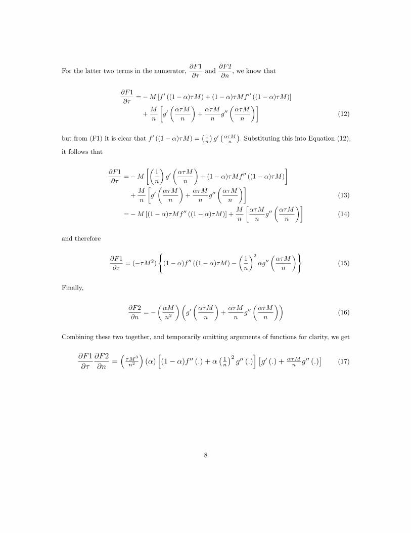
model with a more micro-founded measure of income tax. As we can see from Figure 2, these tax

rate data map neatly to the conventional wisdom.

22

Australia

Austria

Belgium

Canada

Denmark

Finland

France

Germany

Greece

Iceland

IrelandItaly

Japan

LuxembourgNetherlands

New Zealand Norway

Portugal

SpainSweden

Switzerland

UK

USA

010

2030

40A

vera

ge T

ax R

ate

2 4 6 8Parties in Parliament (average)

Tax Rates and Fragmentation (1982--2005)

Figure 2: Relationship with alternative measure of taxation

These additional tax rate data come from Peter, Buttrick and Dundan (2010). This dataset

emphasizes the actual tax rates paid by individuals at specified income levels (average wage, twice

the average wage, etc.) rather than focusing on total receipts of the state. The main variable employed

is the tax rate for the mean income level after adjusting for allowances, credits, local taxes, etc. This

years included are 1982 through 2005.

Again there is a pattern of coefficients changing sign. The result on 4x average income, the

coefficient of which is positive, seems to reject a theme of my model. However, the model does not

make predictions about the progressivity of the tax schedule. The model is about overall tax rates,

and is silent on taxes on higher incomes. Consequently the most useful comparison then is the

difference between Column 1 and Column 2, which measures taxes paid at average income levels.

The results here are consistent with the model. The results with fixed effects are not statistically

23

Table 10: Alternative Tax Measure

Average Income Avg Income x2 Avg Income x4

(1) (2) (3) (4) (5) (6)

Eff. parties 0.921∗∗∗ -0.253 1.097∗∗∗ -0.210 0.988∗∗∗ 0.461

(0.199) (0.349) (0.168) (0.391) (0.254) (0.357)



N 493 493 493 493 493 493


∗ p < 0.10, ∗∗ p < 0.05, ∗∗∗ p < 0.01

significant. This is perhaps not surprising as the inclusion of fixed effects reduces the number of

degrees of freedom by 35. Although they are not significant, they are negative. Furthermore, they

are significantly different from the positive coefficients predicted by excluding fixed effects.

3.6 Different measure of fragmentation

An alternative measure of legislative fragmentation that is closely correlated (but not identical) to

the effective number of parties, was proposed by Rae (1968). This is a nonlinear transformation of

the effective number of parties. If we define the effective number of parties as e, then the Rae measure

equals1

1− e. Table 11 shows the regression output. It would be concerning if this transformation

substantially changed the interpretation of my results.

3.7 Ideological composition

Table 13 shows the effects of including controls for political ideologies. To ensure robustness, I measure

political ideology at both the executive and legislative level. At the executive level, I include the

fraction of cabinet posts held by people of differing political persuasions. At the legislative level,

I control for the fraction of the parliament seats won by a country’s major socialist, conservative,

liberal, and religious parties. Summary statistics are provided in Table 12.

24

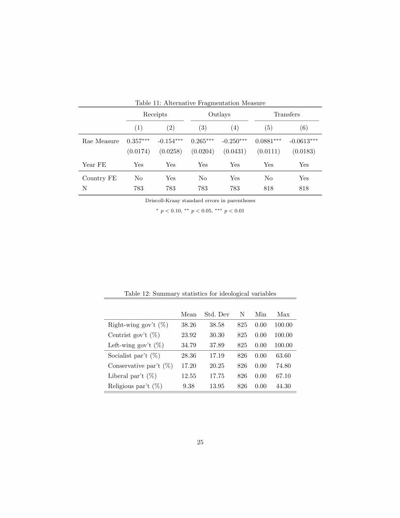
Table 11: Alternative Fragmentation Measure

Receipts Outlays Transfers

(1) (2) (3) (4) (5) (6)

Rae Measure 0.357∗∗∗ -0.154∗∗∗ 0.265∗∗∗ -0.250∗∗∗ 0.0881∗∗∗ -0.0613∗∗∗

(0.0174) (0.0258) (0.0204) (0.0431) (0.0111) (0.0183)



N 783 783 783 783 818 818


∗ p < 0.10, ∗∗ p < 0.05, ∗∗∗ p < 0.01

Table 12: Summary statistics for ideological variables


Right-wing gov’t (%) 38.26 38.58 825 0.00 100.00

Centrist gov’t (%) 23.92 30.30 825 0.00 100.00

Left-wing gov’t (%) 34.79 37.89 825 0.00 100.00

Socialist par’t (%) 28.36 17.19 826 0.00 63.60

Conservative par’t (%) 17.20 20.25 826 0.00 74.80

Liberal par’t (%) 12.55 17.75 826 0.00 67.10

Religious par’t (%) 9.38 13.95 826 0.00 44.30

25

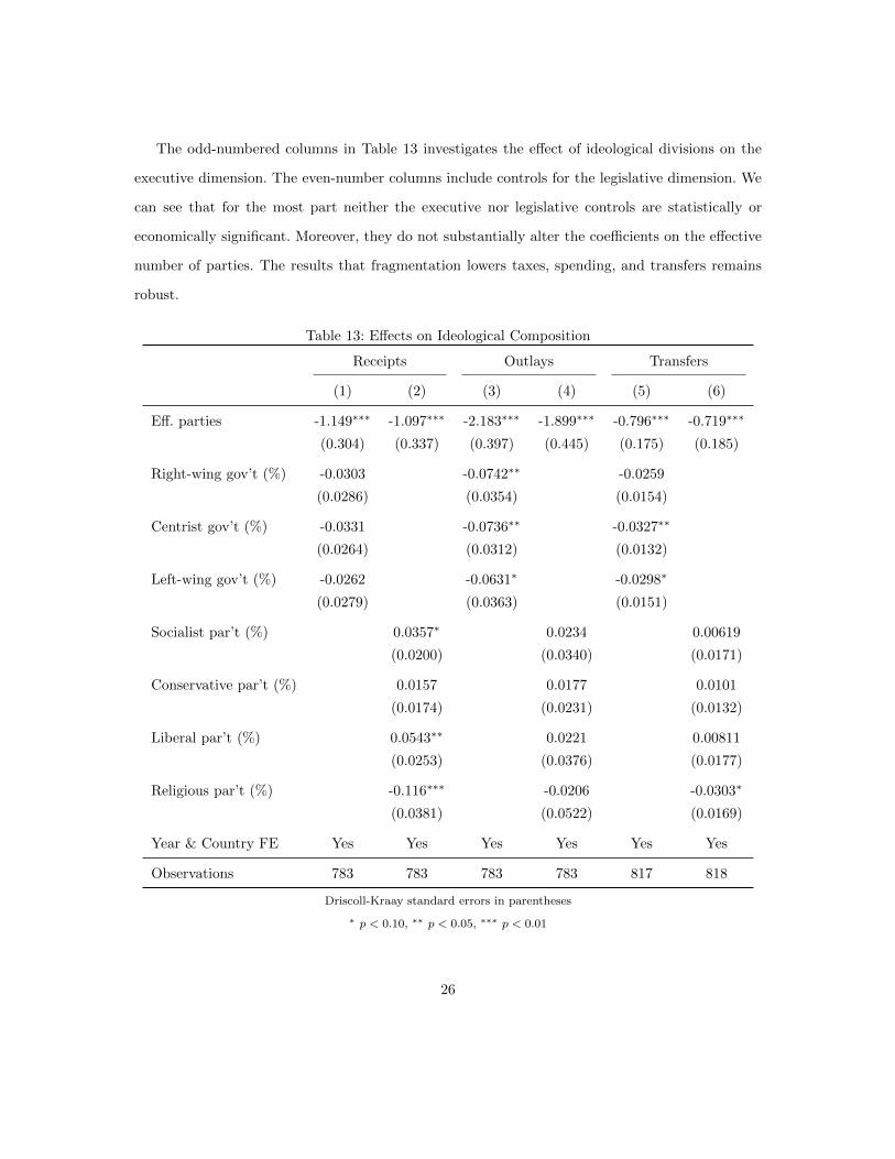
The odd-numbered columns in Table 13 investigates the effect of ideological divisions on the

executive dimension. The even-number columns include controls for the legislative dimension. We

can see that for the most part neither the executive nor legislative controls are statistically or

economically significant. Moreover, they do not substantially alter the coefficients on the effective

number of parties. The results that fragmentation lowers taxes, spending, and transfers remains

robust.

Table 13: Effects on Ideological Composition


(1) (2) (3) (4) (5) (6)

Eff. parties -1.149∗∗∗ -1.097∗∗∗ -2.183∗∗∗ -1.899∗∗∗ -0.796∗∗∗ -0.719∗∗∗

(0.304) (0.337) (0.397) (0.445) (0.175) (0.185)

Right-wing gov’t (%) -0.0303 -0.0742∗∗ -0.0259

(0.0286) (0.0354) (0.0154)

Centrist gov’t (%) -0.0331 -0.0736∗∗ -0.0327∗∗

(0.0264) (0.0312) (0.0132)

Left-wing gov’t (%) -0.0262 -0.0631∗ -0.0298∗

(0.0279) (0.0363) (0.0151)

Socialist par’t (%) 0.0357∗ 0.0234 0.00619

(0.0200) (0.0340) (0.0171)

Conservative par’t (%) 0.0157 0.0177 0.0101

(0.0174) (0.0231) (0.0132)

Liberal par’t (%) 0.0543∗∗ 0.0221 0.00811

(0.0253) (0.0376) (0.0177)

Religious par’t (%) -0.116∗∗∗ -0.0206 -0.0303∗

(0.0381) (0.0522) (0.0169)

Year & Country FE Yes Yes Yes Yes Yes Yes

Observations 783 783 783 783 817 818


∗ p < 0.10, ∗∗ p < 0.05, ∗∗∗ p < 0.01

26

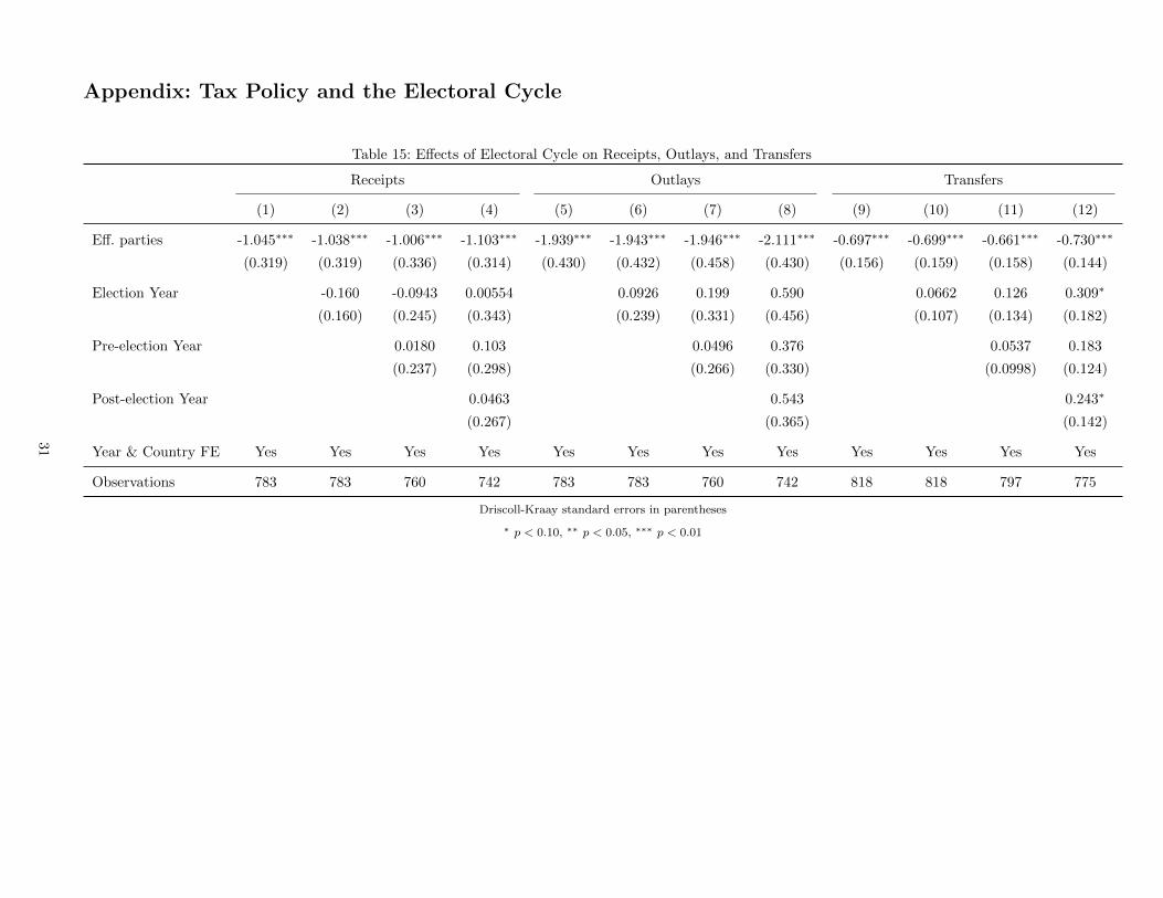
3.8 Electoral cycle

The results are also robust to phases of the electoral cycle. Table 14, which is large and thus left to

the the appendix, illustrates this. I include controls for year before, year of, and year after election.

These results are generally negative but insignificant. They are somewhat significant on receipts:

taxes do indeed go down in an election year. In no specification do the electoral cycle variables

meaningfully alter the main parameters of interest.

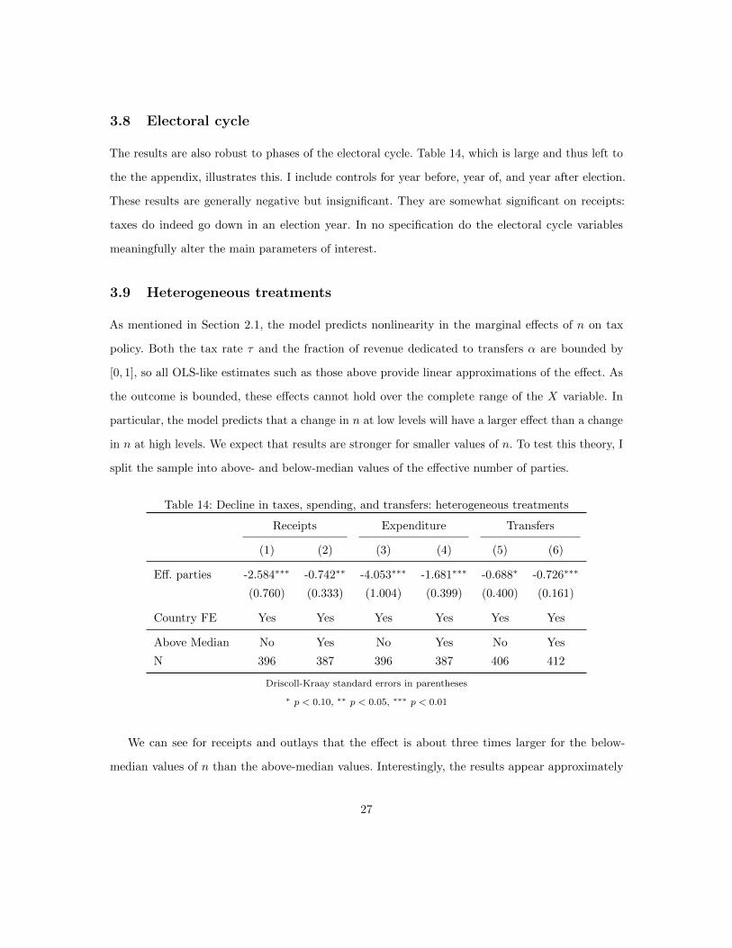
3.9 Heterogeneous treatments

As mentioned in Section 2.1, the model predicts nonlinearity in the marginal effects of n on tax

policy. Both the tax rate τ and the fraction of revenue dedicated to transfers α are bounded by

[0, 1], so all OLS-like estimates such as those above provide linear approximations of the effect. As

the outcome is bounded, these effects cannot hold over the complete range of the X variable. In

particular, the model predicts that a change in n at low levels will have a larger effect than a change

in n at high levels. We expect that results are stronger for smaller values of n. To test this theory, I

split the sample into above- and below-median values of the effective number of parties.

Table 14: Decline in taxes, spending, and transfers: heterogeneous treatments


(1) (2) (3) (4) (5) (6)

Eff. parties -2.584∗∗∗ -0.742∗∗ -4.053∗∗∗ -1.681∗∗∗ -0.688∗ -0.726∗∗∗

(0.760) (0.333) (1.004) (0.399) (0.400) (0.161)

Country FE Yes Yes Yes Yes Yes Yes

Above Median No Yes No Yes No Yes

N 396 387 396 387 406 412


∗ p < 0.10, ∗∗ p < 0.05, ∗∗∗ p < 0.01

We can see for receipts and outlays that the effect is about three times larger for the below-

median values of n than the above-median values. Interestingly, the results appear approximately

27

constant for transfers. I conclude that there is strong evidence of nonlinearity in effects on receipts

and outlays, but no such evidence for transfers.

4 Conclusion

This paper asks how political fragmentation affects fiscal policy outcomes. I modeled this as a common

pool problem. This common pool problem presents a coalition which simultaneously chooses tax and

expenditure policies. Unlike other models which constrain the coalition’s actions through norms, the

coalition’s choice essentially corresponds to a group welfare maximization problem. The coalition can

fund two types of good: the pure public good which is shared by all, and the local public good which

is targeted to political constituencies. Comparative static analysis indicates that taxes, spending,

transfers, and transfer intensity fall as the coalition becomes more fragmented.

The contributions of this paper are twofold. Firstly, it supports the empirical result of Pettersson-

Lidbom (2012) with greater external validity than quasi-experimental settings can provide. The

selection of data from a panel of developed nations lends the empirical section to a battery of robust-

ness tests. The results are robust to different specifications, measures of executive fragmentation,

alternative data sources, ideological controls, and electoral cycle effects. Secondly, the paper provides

a general theoretical foundation that motivate these results. The conventional wisdom in the litera-

ture is that more fragmented governments lead to larger public sectors. Both the theoretical and

empirical sections suggest that the conventional wisdom is incorrect. The model in Section 2 could

be extended to incorporate more nuance in the effect of fragmentation on legislative bargaining.

This is an avenue for future work.

28

References

Alesina, A., Devleeschauwer, A., Easterly, W., Kurlat, S. and Wacziarg, R. (2003) Fractionalization,

Journal of Economic Growth, 8, 155–194.

Armingeon, K., Careja, R., Weisstanner, D., Engler, S., Potolidis, P. and Gerber, M. (2012a) Com-

parative Political Data Set III 1990-2010, Bern: Institute of Political Science, University of Bern.

Armingeon, K., Weisstanner, D., Engler, S., Potolidis, P. and Gerber, M. (2012b) Comparative

Political Data Set I 1960-2010, Bern: Institute of Political Science, University of Bern.

Austen-Smith, D. (2000) Redistributing income under proportional representation, Journal of Po-

litical Economy, 108, 1235–1269.

Driscoll, J. C. and Kraay, A. C. (1998) Consistent covariance matrix estimation with spatially

dependent panel data, Review of Economics and Statistics, 80, 549–560.

Hall, P. A. and Soskice, D. W. (2001) Varieties of Capitalism: The institutional foundations of

comparative advantage, vol. 8, Oxford University Press.

Kontopoulos, Y. and Perotti, R. (1999) Government Fragmentation and Fiscal Policy Outcomes:

Evidence from OECD Countries, in Fiscal Institutions and Fiscal Performance, National Bureau

of Economic Research, NBER Chapters, pp. 81–102.

Lijphart, A. (1984) Democracies: Patterns of majoritarian and consensus government in twenty-one

countries, New Haven: Yale University Press.

Lijphart, A. (1999) Patterns of Democracy: Government forms and performance in thirty-six democ-

racies, New Haven: Yale University Press.

Mendoza, E. G., Razin, A. and Tesar, L. L. (1994) Effective tax rates in macroeconomics: Cross-

country estimates of tax rates on factor incomes and consumption, Journal of Monetary Economics,

34, 297–323.

29

Milesi-Ferretti, G. M., Perotti, R. and Rostagno, M. (2002) Electoral systems and public spending,

The Quarterly Journal of Economics, 117, 609–657.

Newey, W. K. and West, K. D. (1994) Automatic lag selection in covariance matrix estimation, The

Review of Economic Studies, 61, 631–653.

Persson, T. and Tabellini, G. (2002) Political Economics: Explaining Economic Policy, MIT Press.

Peter, K. S., Buttrick, S. and Dundan, D. (2010) Global reform of personal income taxation, 1981-

2005: Evidence from 189 countries, National Tax Journal, 63, 447–478.

Pettersson-Lidbom, P. (2012) Does the size of the legislature affect the size of government? Evidence

from two natural experiments, Journal of Public Economics, 96, 269–278.

Rae, D. (1968) A note on the fractionalization of some European party systems, Comparative

Political Studies, 1, 413–418.

Tsebelis, G. (2002) Veto Players: How political institutions work, Princeton University Press.

Weingast, B. R., Shepsle, K. A. and Johnsen, C. (1981) The political economy of benefits and costs:

A neoclassical approach to distributive politics, The Journal of Political Economy, pp. 642–664.

30

Appendix: Tax Policy and the Electoral Cycle

Table 15: Effects of Electoral Cycle on Receipts, Outlays, and Transfers


(1) (2) (3) (4) (5) (6) (7) (8) (9) (10) (11) (12)

Eff. parties -1.045∗∗∗ -1.038∗∗∗ -1.006∗∗∗ -1.103∗∗∗ -1.939∗∗∗ -1.943∗∗∗ -1.946∗∗∗ -2.111∗∗∗ -0.697∗∗∗ -0.699∗∗∗ -0.661∗∗∗ -0.730∗∗∗

(0.319) (0.319) (0.336) (0.314) (0.430) (0.432) (0.458) (0.430) (0.156) (0.159) (0.158) (0.144)

Election Year -0.160 -0.0943 0.00554 0.0926 0.199 0.590 0.0662 0.126 0.309∗

(0.160) (0.245) (0.343) (0.239) (0.331) (0.456) (0.107) (0.134) (0.182)

Pre-election Year 0.0180 0.103 0.0496 0.376 0.0537 0.183

(0.237) (0.298) (0.266) (0.330) (0.0998) (0.124)

Post-election Year 0.0463 0.543 0.243∗

(0.267) (0.365) (0.142)

Year & Country FE Yes Yes Yes Yes Yes Yes Yes Yes Yes Yes Yes Yes

Observations 783 783 760 742 783 783 760 742 818 818 797 775


∗ p < 0.10, ∗∗ p < 0.05, ∗∗∗ p < 0.01

31

political fragmentation and fiscal policy - ntanet.org · political fragmentation and fiscal policy...

Documents