polluting non-renewable resources, innovation and growth
TRANSCRIPT

Polluting Non-Renewable Resources, Innovation and
Growth: Welfare and Environmental Policy
André Grimaud1 and Luc Rougé2
August 2003
1Université de Toulouse 1 (GREMAQ, IDEI and LEERNA), 21 allée de Brienne, 31000Toulouse, France, and ESCT. E-mail: [email protected]
2ESCT and Université de Toulouse 1 (GREMAQ and LEERNA). E-mail: [email protected]

Abstract
We analyze the impact of the pollution generated by the use of non-renewable resources
on the standard results of growth models. In this context, we obtain a Hotelling rule
which is not a pure efficiency condition any longer. Subsequently, we show that some of
the optimal paths’ standard properties change: in particular, an increase in the house-
holds’ psychological discount rate leads to a slower extraction of the resource. Moreover,
we present a simple endogenous growth model that allows us to study the effects of an
environmental policy aimed at correcting the distortion introduced at the equilibrium. We
show that the tax level does not matter, and that a decreasing tax on the resource use
yields the optimum.
Keywords: non-renewable resources, pollution, innovation, growth, extraction path,
environmental policy.
JEL classification: O32, O41, Q20, Q32

1 Introduction
When considering the standard analysis of economic growth in the presence of non-
renewable natural resources, the main questions that arise are the following. Is positive
long term growth possible despite the fact that one of the production process’ inputs is
only available in a finite quantity? What is the optimal growth path (namely, what is
the optimal rate of resource extraction)? What is the equilibrium path? What are its
properties, in particular, is it optimal?
The literature has answered these questions through two main types of models: the
Ramsey growth model (where we can quote Stiglitz (1974), Garg and Sweeney (1978) or
Dasgupta and Heal (1979)) and the endogenous growth models (Schou (1996), Aghion and
Howitt (1998), Scholz and Ziemes (1999), Barbier (1999) or Grimaud and Rouge (2003)).
Both kinds of models show that long-term positive growth is possible under certain tech-
nological conditions. In the former, the key optimality point is given by Hotelling’s rule,
an efficiency condition that characterizes the optimal resource extraction rate. It says that
the marginal productivity of capital must equal the growth rate of the resource’s marginal
productivity. At market equilibrium, one of the conditions implies that the growth rate of
the resource’s price must equal the interest rate. As competition is assumed to be perfect
in all markets, the unit prices of capital and of the resource must be respectively equal
to their marginal productivities. Therefore, Hotelling’s rule is verified at the equilibrium,
and the equilibrium and optimal paths are identical.
In the second type of models, whether we consider those with horizontal (Romer) or
vertical (Aghion-Howitt) differentiation, the optimal paths are in general not followed by
the market equilibrium -a feature essentially due to intertemporal externalities that arise
from the fact that knowledge is a public good, and to the mark-up imposed by monopolies
that sell the intermediate goods.
A common feature of the papers cited above is that they neglect a key characteristic of
nearly all non renewable resources that are presently used (fossil fuels / mineral resources).
Indeed, the combustion of petroleum, coal and, to a lesser extent, natural gas is responsible
for an important part of CO2, the main greenhouse gas (and also SOx and NOx causes of
1

acid rain) -and thus responsible for an eventual climatic change. A part of the literature has
already incorporated this aspect when considering the problem of non-renewable resources.
Kolstad and Krautkraemer (1993) realise a survey of this literature. More recently, we can
quote for example Tahvonen’s (1997 and 2001) or Schou’s (2000 and 2002) contributions.
The latter uses Uzawa-Lucas and Romer-type growth models to consider the problem ; we
will refer to his results further below.
When polluting emissions are a by-product of the use of non-renewable resources,
several questions arise. One can first ask whether the emissions thus generated constitute
a stock or a flow. Several elements may lead to believe that pollution must be treated as a
stock variable. Indeed, though carbon dioxide emissions are retained by the atmosphere,
a part of these is also seized by oceans (and forests) and trapped for long periods of time.
It therefore appears that a dynamic analysis of their effects is required. However, the fact
that this can sensibly complicate calculations must also be taken into account. We will
see further on that the growth model we develop initially incorporates two state variables
(the stocks of knowledge and resource), and that the analysis of the stock of pollution
requires us to incorporate a third one. Yet, as Kolstad and Krautkraemer (1993) put it:
”in general, it is difficult or impossible to characterize the qualitative features of a model
with three state variables without restrictive assumptions about the functional forms of
important relationships”. For the preceding reason we will treat pollution uniquely as a
flow, as was done for example in Schou (2000), keeping in mind that it is only a first step
in the analysis.
Another major question concerns the effects generated by this pollution. In fact, we
can assume that it affects two targets in particular: the production process and households’
utility. In the first case, for example, its effects could be an increased depreciation of capital
due to air pollution. Schou (2000) focuses on this case. Here, we will only consider the
effects on the second target (pollution reduces household’s utility), because it appears to
be more straightforward, and because it is the subject of a great part of the literature (see
for example Smulders and Gradus (1993) or Aghion and Howitt (1998)). Note, however,
that the simultaneous analysis of both effects is a line of research to be considered in the
future.
2

We therefore introduce an endogenous growth model with Romer horizontal differen-
tiation in the presence of non-renewable resources whose use in the production process
generates a flow of pollution that negatively affects households’ utility. It is then clear
how our problem differs from the problem posed by the standard growth models with
non-renewable natural resources presented above. Indeed, the question before was: how
should a finite stock of resources be distributed among an infinite set of generations? Now,
a supplementary question is added to the problem: how to distribute the associated finite
stock of pollution among an infinite set of generations? By introducing an externality
linked to the use of the resource, we have added an additional dimension to the problem:
the choice of an extraction path now implies the simultaneous choice of a pollution path.
We can thus imagine that the resource’s optimal extraction rate will be modified ; we will
see, for example, that the disutility created by pollution appears in the optimality condi-
tions, and we will obtain a non-standard version of the Hotelling rule. We then go on to
specify functional forms and we characterize the steady state solutions. In particular, we
obtain that higher household preferences for the present imply a slower resource extraction
rate, a result contrary to that obtained by the standard literature (see Stiglitz (1974) for
example).
Next we adopt a particular type of economic decentralization. Given that our main
objective is to concentrate on the consequences of introducing pollution into the standard
theory of non-renewable resources, we eliminate all other distortions in order to isolate
its effects. In so doing, we also wish to avoid some of the technical difficulties that are
usually associated with this kind of models. Our endogenous growth model therefore has
no intermediate goods, and we assume that innovations are indivisible public goods di-
rectly financed by patents. Naturally, such a characterization of decentralization cannot
be considered as a reference equilibrium (we will come to this later), but we believe it is
interesting for the reasons discussed above. We then show the differences between equilib-
rium and optimal conditions and we interpret this non-optimality. Next, we characterize
the equilibrium steady state and, namely, we show that resources are extracted too rapidly
(with respect to the optimal rate) and that the equilibrium level of R&D is under optimal.
Finally, we implement an environmental policy aimed at correcting the model’s sole
3

distortion, which arises from the polluting emissions generated by the use of the resource.
The policy is a unit tax on resource purchases. Contrary to Schou (2002), we show that
such an instrument is necessary in order to correct equilibrium conditions and bring them
closer to optimality. Moreover, our analysis indicates that it is the tax’s growth rate, and
not its level, which allows the distortion to be corrected. We then analyze the effects of
this policy on the model’s variables and we define the tax’s optimal growth rate, that is,
the rate which makes the equilibrium path become an optimal one.
In the section that follows, we present the model and the welfare analysis. We define
the economy’s market equilibrium and present its properties in section 3. Then, in section
4, we study the effects of the environmental policy and we characterize the optimal policy.
Finally, we give concluding remarks in section 5.
2 Presentation of the model and welfare analysis
2.1 The model
We first present a non specified version of the model in order to get general characteristic
conditions at optimum (section 2.2) and equilibrium (3.1), and to compare them.
At each time t, a quantity Yt of homogeneous good is produced according to the
following technology:
Yt = F (LY t, At, Rt), (1)
where LY t is the amount of labour devoted to production, At is the stock of knowledge
and Rt is the flow of non-renewable resource used within the production process. We will
denote by FL, FA and FR the marginal productivities.
We consider that each innovation is a public, indivisible and infinitely durable good,
which is simultaneously used by the homogeneous good sector and the R&D sector 1.
Formally, it is a point of the segment [0, At]. At each time t, the stock of knowledge
1For instance, we think of a scientific report in which is described a new theory which can be usedwithin the production process.
4

evolves as follows:
At = q(At, LRDt), (2)
where LRDt is the amount of labour devoted to R&D. We will denote by qA and qL
the marginal productivities. Note that the flow of knowledge depends on the pre-existing
stock.
Remark: In this model, contrarily to what is done in the standard endogenous growth
literature (see for instance Aghion-Howitt (1992), Grossman-Helpman (1991), or Romer
(1990)), knowledge is not embodied inside intermediate goods.
We suppose that the technologies F () and q() exhibit constant returns to scale in
private inputs, that is, F (λLY , A,λR) = λF (LY , A,R) and q(A,λLRD) = λq(A,LRD).
This assumption is justified by the standard replication argument: see for instance Romer
(1990) or Jones (2001).
Population is assumed constant, normalized to one, and each individual is endowed
with one unit of labour. Thus we have:
1 = LY t + LRDt. (3)
The resource is extracted from a initial finite stock S0, and we have the standard
resource stock law of motion:
St = −Rt. (4)
The whole production of homogeneous good is consumed by the representative house-
hold:
Yt = Ct. (5)
The household instantaneous utility function depends both on consumption Ct and on
5

the flow of pollution Pt. We write the intertemporal utility function as follows:
U0 =
Z +∞
0u (Ct, Pt) e
−ρtdt, (6)
where the partial derivatives of the utility function with respect to consumption and
pollution are denoted by UC and UP and are positive and negative respectively.
Pollution is generated by the use of the non-renewable natural resource within the
production process:
Pt = h(Rt), with h0 > 0. (7)
2.2 Welfare analysis
The social planner maximizesR +∞0 u (Ct, Pt) e
−ρtdt subject to (1), (2), (3), (4), (5) and
(7).
After elimination of the co-state variables, the first order conditions reduce to the two
following characteristic conditions (we drop time subscripts for notational convenience):
ρ− UCUC
=FLFL− qLqL+FAqLFL
+ qA (8)
and
FRFR
+ (
•UPh
0 − ρUPh0
UCFR) =
FLFL− qLqL+FAqLFL
+ qA. (9)
Proof. See Appendix A.
Equations (8) and (9) are versions of the Ramsey-Keynes and Hotelling rules respec-
tively2. There are three differences with the standard formulations. First, contrary to
the standard neo-classical growth model, we do not have physical capital but a stock At
of knowledge: this explains that the marginal productivity of capital is replaced by the
RHS in (8) and (9). The relative complexity of this expression comes from the fact that
a variation of Ct is compensated by a transfer of labor between the consumption good
2A complete economic interpretation of these two conditions is available from the authors upon request.
6

sector (LY ) and the research sector (LA) which modifies the whole trajectory of variable
At. The second difference is that in (8), UC is equal to UCCC + UCP P (UCP is nil in the
case of a non-separable utility function). Third, the Hotelling rule is no longer strictly a
pure efficiency condition as in the standard model without pollution (see Withagen (1999),
p 52). Indeed, extracting one unit of resource allows to produce more (this is standard),
but this also entails an increase in pollution, which creates a disutility. This explains the
term between brackets in (9).
2.3 Specification and steady-state analysis
2.3.1 Steady-state optimum: characterization and existence
In order to go further in the analysis, and later to study the effects of a green tax, we
consider the following standard specifications. As mentioned above, production and R&D
technologies exhibit constant returns to scale in private inputs:
Yt = LαY tR
1−αt Aν
t , with 0 < α < 1 and ν > 0, (10)
At = δLRDtAt, with δ > 0. (11)
We assume that emissions are a linear function of extraction flows:
h (Rt) = γRt, with γ > 0. (12)
Finally we take the separable instantaneous utility function used by Aghion and Howitt
(Chapter 5, 1998) for example:
and u(Ct, Pt) =C1−εt
1− ε− P
1+ωt
1 + ω, with ε > 0 and ω > 0. (13)
Characterization:
We focus now on the study of steady-state paths, i.e., on paths along which the growth
7

rate of any variable is constant.
Proposition 1 At the steady-state optimum, the quantities and growth rates take the
following values (we denote gz the growth rate of any variable z, we use upper-script o for
optimum, and we drop time subscripts for notational convenience):
LoRD =(δν − ρα)(ε(1− α) + α+ ω)
δν(ε+ ω(1− α+ εα)), (14)
LoY = 1− LoRD, (15)
goA = δLoRD, (16)
goR = goP = g
oS =
(δν − ρα) (1− ε)
ε+ ω(1− α+ εα), (17)
goC = goY =
(δν − ρα) (1 + ω)
ε+ ω(1− α+ εα). (18)
Remark: At the steady-state optimum, given S0 and A0, the initial quantities are
Y o0 = Co0 = (L
oY )
α(−S0goR)1−α(A0)ν , Ro0 = P o0 /γ = −S0goR (dividing (4) by St yields thisresult), and at each time t we have xot = x
o0egoxt for any variable x.
Proof. Applying the specifications (10), (11), (12) and (13) to (8) and (9), and
considering that all rates of growth are constant, the result follows.
Existence of interior optimum:
The two transversality conditions of the social planner’s program are respectively
limt→+∞µtA
ot e−ρt = 0 and lim
t→+∞νtSot e−ρt = 0, and they imply LoRD < 1 and goR < 0
respectively (see Appendix C for details). Moreover, we need LoRD > 0 to have a solution.
The three conditions are together fulfilled if ε > 1 and ρ < δν/α (see equations (14), (15)
8

and (17))3. Note that on this set of parameters values, we have goY > 0 (see (18)). These
results are summarized in Figure 1.
ρ αδν /
Optimum exists only if 1>ε
Then 0>oYg
Optimum does not exist.
0
Figure 1: Existence of interior optimum
2.3.2 Properties of the optimal path
We now perform some comparative statics so as to describe the main properties of the
path we just defined, and to compare it with what has been obtained in more standard
growth models. Letters S and GR indicate that similar results have been obtained by
Stiglitz (1974) and Grimaud-Rouge (2003), respectively in a ”à la Ramsey” and a ”à la
Aghion-Howitt” standard models with a non-renewable resource (which does not pollute).
3Similar conditions are obtained by Aghion-Howitt (1998) in a ”Schumpeterian Approach to Pollution”,p 161.
9

ξ = δ ξ = ε ξ = ρ ξ = ν ξ = ω
∂LoRD∂ξ
> 0 < 0 < 0 > 0 < 0
GR GR GR
∂goA∂ξ
> 0 < 0 < 0 > 0 < 0
GR GR GR
∂goR∂ξ
< 0 < 0 > 0 < 0 > 0
S,GR S,GR
∂goY∂ξ
> 0 < 0 < 0 > 0 > 0
S,GR S,GR S,GR
Table 1: Properties of the optimal path
• The effects of a change in δ or ε on the variables of the model are quite standard. Inour model, δ is a parameter which characterizes the effectiveness of the R&D sector,
and it can be seen as the exogenous part of technological progress: it corresponds to η
in Stiglitz. A higher δ means that devoting labour to research is better, hence labour
in research (LoRD) and the growth rate of knowledge (goA) grow. This will increase
the output growth rate, despite a lower resource extraction growth as in Stiglitz and
Grimaud-Rouge. On the reverse, an increase in the elasticity of marginal utility,
ε, means that more utility is derived from uniform consumption paths. That is
why a social planner will invest less in R&D (LoRD and goA decrease). Moreover,
this planner will lower consumption growth and therefore choose a lower resource
extraction growth rate goR (we have the same result in Stiglitz and Grimaud-Rouge).
• Here, taking into account the pollution emitted by the use of the non-renewableresource modifies the impact of a change in ρ (the psychological discount rate) on
goR, with respect with the standard literature.
10

An increase in ρ means that utility derived from current times are more valued
relative to utility derived from future times. In the literature mentioned above, this
implies that the representative household values more current consumption relative
to future consumption. Thus the steady-state growth rate of the output will decrease,
which corresponds to more output today and less tomorrow (relative to the situation
before the increase in ρ). In order to produce more today, the social planner will
increase the amount LoY of labour and the flow Ro of resource both used within the
production process. An increase in the ”production-labour” today means a decrease
in the ”R&D-labour” today, thus a decrease in the growth rate of knowledge (see
(2)). An increase in the flow of resource used today implies a decrease in the flow
used tomorrow: goR decreases.
In our framework, the fundamental difference comes from the fact that valuing more
utilities derived from current times does not only mean valuing more current con-
sumptions. This also means valuing more the current states of the environment (see
(6)): improving the first generations’s welfare means also improving their environ-
ment. Thus P o0 (i.e. Ro0) must decrease. So, as above, the planner will increase
LoY today, that is, decrease LoRD and thus decrease goA; but at the same time, the
planner will decrease the level of pollution today, and increase this level tomorrow
(recall that, in our framework, the stock of pollution is finite): that is why, contrarily
to what is obtained in models without pollution, goP (that is, goR) increases.
• A higher ω corresponds to an increase in the household’s care for the cleanliness
of the environment. One fundamental feature of our model, as we just recalled, is
that pollution is created by the use of a non-renewable resource. That is why the
stock of pollution is finite; for this reason, at the steady-state, polluting more (resp.
less) today means polluting less (resp. more) in the future. Thus, for a given time
preference, an increase in ω implies less pollution today and more tomorrow. Hence,
at the steady-state, the optimal growth rate of the resource extraction will increase:
less resource is consumed today (i.e. less pollution is emitted) and more tomorrow
(i.e. more pollution tomorrow). To compensate the fall in Ro0, the planner will have
11

to increase LoY today, and thus to decrease LoRD; that is why the growth rate of
knowledge decreases. From (10), we have goY = (1−α)goR+ νgoA at the steady-state.
It turns out that the combination of both effects (a rise in goR and a fall in goA) results
in a domination of the former: goY increases.
So, the more households will value their environment, the slowlier the resource will
be extracted, and the more rapidly output will grow.
Remark: With a non-separable utility function (as in Schou (2002)), one could not
disentangle the effects of ω and ρ. For instance, a higher ρ would lead to a slower
extraction provided that households care enough for their environment.
3 Decentralized equilibrium
3.1 Behaviour of agents and equilibrium conditions
Let us consider the non-specified version of the model presented in section 2.1. The price
of good Y is normalized to one, and wt, pRt and rt are, respectively, the wage, the resource
price, and the interest rate on a perfect financial market. In order to eliminate the market
failure arising from the fact that firms do not take into account the negative externality
due to the use of the non-renewable resource within the production process , i.e., pollution,
we use a policy tool: a tax on the demand of resource.
Remark: Here we do not tax Pt but Rt. Indeed, since Pt and Rt are linked by a func-
tional relation, we can implement the optimum by only taxing the resource use. Moreover,
it is generally more convenient to observe the quantity of resource and thus to use such a
policy design.
Homogeneous good sector:
At each time t, the profit of the firm is
πYt = F (LY t, At, Rt)− wtLY t − pRt(1 + σt)Rt (19)
where σt is the unit tax on the resource use. From now on, we will note τ t = 1 + σt for
12

computational convenience.
Differenciating πYt with respect to LY t and Rt, and equating to zero, gives the two
following first order conditions:
FL = wt, (20)
and FR = τ tpRt. (21)
R&D sector:
As we mentioned above, knowledge is not embodied inside intermediate goods, thus it
cannot be financed by the sale of these goods. We suppose here that knowledge is directly
financed. Nonetheless, as the sectors using knowledge exhibit constant returns to scale
in the private goods, their profits are nil; thus we assume that once an innovation has
occured, the government pays to the innovator a sum equal to the willingnesses to pay of
both sectors.
Remark: This type of decentralization defines an equilibrium that is a benchmark: in
the absence of any pollution, this equilibrium is a first best optimum (as we will show it
below). This is a formalization of ideas already expressed by Arrow (1962), Dasgupta et al.
(1996) or Scotchmer (1991 and 1999). The main interest of designing such an equilibrium
is that it allows us to focus on one single distorsion: the one caused by pollution. Hence
we avoid the distorsions (monopolies rents, intertemporal spillovers...) inherent to the
equilibria used in the standard endogenous growth models. Indeed, these distorsions
entail a useless complexity of the model. Note that, as seen above, considering such an
equilibrium leads to assume that the governement finances entirely R&D. However, it is
possible, assuming that the two sectors using innovations (final sector and R&D sector)
are imperfectly competitive, to construct an equilibrium in which R&D is entirely and
privately financed by these sectors (we find a similar equilibrium path in this case).
13

At each time t, the value of an innovation is:
Vt =
Z +∞
0vse
− R st rududs, (22)
where vs is the sum of the willingnesses to pay of the homogeneous good sector (vYs )
and the R&D sector (vRDs ): vs = vYs + vRDs .
The profit on innovations produced at t is:
πRDt = q(At, LRDt)Vt − wtLRDt (23)
The maximization of this profit function with respect to LRt leads to the following first
order condition:
qLVt = wt (24)
From (19) and (23), we have:
vYt =∂πYt∂At
= FA
and vRDt =∂πRDt∂At
= qAVt,
which gives
vt = FA + qAVt. (25)
Representative household:
At each time t, the representative household maximizes the utility functionR +∞0 u (Ct, Pt) e
−ρtdt
subject to Bt = wt + rtBt + pRtRt − Tt − Ct, where Bt is the stock of bonds at t, and Ttis a lump-sum tax levied by the government to finance research. This maximization leads
14

to the following condition:
ρ− UCCC + UCP PUC
= rt. (26)
Resource sector:
On the competitive natural resource market, the maximization of the profit functionR +∞t pRsRse
− R st rududs, subject to Ss = −Rs, Ss ≥ 0, Rs ≥ 0, s ≥ t, yields the standardequilibrium ”Hotelling rule”:
pRtpRt
= rt, for all t. (27)
Observe that, since pRt = FR in absence of environmental policy (see (21) above), it
is clear that here, the decentralized economy does not implement the optimum Hotelling
rule given by (9) (we come back to this point later in the text).
Government:
The government’s budget constraint is4
Tt + σtpRtRt = vYt + v
RDt , for all t.
Our objective is now to exhibit the two characteristic equilibrium conditions that can
be compared to the optimum ones ((8) and (9)). We obtain:
ρ− UCCC + UCP PUC
=FLFL− qLqL+FAqLFL
+ qA (28)
and
FRFR− τ t
τ t=FLFL− qLqL+FAqLFL
+ qA (29)
4We assume here that the government possesses all the information and thus can perfectly determinevY and vRD. Of course this is just a benchmark and informational asymmetries could be introduced.
15

Proof. Differentiating (22) and (24) with respect to time gives wtwt= rt − vt
Vt+ qL
qL.
Using (20), (24) and (25), we get: rt =FLFL− qLqL+ FAqL
FL+ qA. This equation, together with
(26) gives (28).
The same equation together with (21) and (27) leads to (29).
First of all, we can observe that (8) and (28) are identical: in other words, at the
equilibrium, the optimum Ramsey-Keynes rule is verified.
However, we can see (compare (9) and (29)) that in absence of any environmental
policy, the optimum Hotelling rule is not verified. This comes from the fact that the social
cost of pollution is not reflected in the resource price. We analyse this point in section
4 and we show that it implies that the resource is extracted too fast at the equilibrium.
Nonetheless, if pollution has no impact on the utility of households (UP = 0), equations
(9) and (29) are identical and the first best optimum is reached, as mentioned above (see
the remark after (21)).
3.2 Specification and steady-state analysis
3.2.1 Steady-state equilibrium: characterization and existence
Now we use the specifications (10), (11), (12) and (13) presented in section 2.3.1, and here
also we focus on steady-state paths.
Characterization:
Proposition 2 At the steady-state equilibrium, the quantities and rates of growth take
the following values (the upper-script e is used for equilibrium):
LeRD =(ε− αε+ α)δν − αρ+ α(ε− 1)(1− α)gτ
εδν, (30)
LeY = 1− LeRD, (31)
geA = δLeRD, (32)
16

geR = geP = g
eS =
δν (1− ε)− ρ
ε+
α− 1− αε
εgτ , (33)
geC = geY =
δν − ρ
ε− 1− α
εgτ . (34)
Remark: At the steady-state equilibrium, given S0 and A0, the initial quantities are
Y e0 = Ce0 = (LeY )α(−S0geR)1−α(A0)ν , Re0 = P e0 /γ = −S0geR, and at each time t we have
xet = xe0egext for any variable x.
Proof. Applying the specifications (10), (11), (12) and (13) to (28) and (29), and
considering that all rates of growth are constant, the result follows.
At the equilibrium steady-state, prices are:
wt = α(LeY )α−1(Ret )
1−α(Aet )ν , (35)
pRt = (1− α)(LeY )α(Ret )
−α(Aet )ν(τ0e
gτ t)−1, (36)
and r = δν−(1−α)gτ , vYt = ν(LeY )α(Ret )
1−α(Aet )ν−1, vRDt = LeRDα(LeY )
α−1(Ret )1−α(Aet )ν−1,
Vt = (α/δ)(LeY )
α−1(Ret )1−α(Aet )ν−1, where Ret = −Se0geRegeRt and Aet = A
e0egeAt.
Existence of interior equilibrium:
Within this analysis, we suppose that there is no environmental policy, that is, τ t = 1
(or equivalently, σt = 0).
As we did for the optimal path, we are looking for the set of parameter values in which
0 < LeRD < 1, and geR < 0. To do so, we use equations (30) and (33). The set is described
in Figure 2:
3.2.2 Equilibrium properties
As it is done for the optimum, we now study the impact of different exogenous parameters
variations on LeRD, geA, g
eR and g
eY . The results are depicted in Table 2.
Letters GR indicate that similar results have been obtained by Grimaud-Rouge (2003)
17

ρ
Equilibrium exists
0
0>oYg
Equilibrium does not exist.
Equilibrium does not exist.
Case 1 : ε < 1 αδνααεε /)( +−δν
ρ
Equilibrium exists
0
0>oYg 0<oYg
Equilibrium does not exist.
Case 2 : ε > 1 δν αδνααεε /)( +−
ε−1
0<oYg
Figure 2: Existence of interior equilibrium
in a model ”à la Aghion-Howitt” with a non-polluting non-renewable resource.
ξ = δ ξ = ε ξ = ρ ξ = ν ξ = ω
∂LeRD∂ξ
> 0 < 0 < 0 > 0 = 0
GR GR GR
∂geA∂ξ
> 0 < 0 < 0 > 0 = 0
GR GR GR
∂geR∂ξ
< 0 < 0 < 0 < 0 = 0
if ε > 1 if geY > 0 if ε > 1
GR GR GR
∂geY∂ξ
> 0 < 0 < 0 > 0 = 0
if geY > 0
GR GR GR
Table 2: Properties of the equilibrium path
The effects of the parameters variations presented in Table 2 result from market mech-
18

anisms (in Table 1, they resulted from the planner’s decisions). We can see that the
properties of the equilibrium path are very similar to the properties of the optimal one.
There are only two differences. First, geR is an decreasing function of ρ. Indeed, if ρ gets
higher, households derive more utility from current consumption, thus want to consume
more today: geC decreases. Hence firms will produce more today and less tomorrow. In
order to increase the output today, they will use more inputs: more labour and more re-
source. Indeed, contrarily to the social planner, firms do not take into account the effects
of the resource use on the utility of consumers. As more resource is extracted today, the
stock being finite, less will be extracted tomorrow: geR decreases. The second difference
with the properties of the optimal path is that ω has no effect on the equilibrium variables.
Indeed this parameter represents the taste of households for their environment (or equiva-
lently their vulnerability towards pollution); however, in the absence of any environmental
policy, pollution is not priced in this model, thus ω affects no market.
4 Impact of the environmental policy and implementation
of the optimum
4.1 Optimum versus equilibrium
First of all, Figure 1 and Figure 2 show that both the optimal path and the equilibrium
path are defined together if ε > 1 and ρ < δν/α. Thus, as we want to compare these paths
and to analyse the effects of an environmental policy, one of the main goals of which is
the implementation of the optimum, this conditions will hold throughout the remainder
of this section.
Proposition 3 In absence of any environmental policy, we have:
LeRD > LoRD, (37)
geR < goR, (38)
19

geY < goY . (39)
Proof. In the set of parameter values described above, we compare LeRD (see (30))
and LoRD (see (14)), geR (see (33)) and g
oR (see (17)), and g
eY (see (34)) and g
oY (see (18)).
The results follow.
In this model, there is one single distorsion: the pollution emitted by the resource use.
If there is no pollution (or equivalently if consumers do not value their environment), the
decentralized equilibrium is a first best optimum (see above). If there is pollution, but
no tax, the equilibrium remains unchanged because firms do not take into account this
pollution: this equilibrium remains equivalent to the first best without pollution.
Hence, comparing the equilibrium (without any public intervention) and the optimal
paths is exactly the same as comparing the optimal path in the absence of pollution and
the optimal path when the resource use yields a flow of pollution that affects negatively
consumers’utility.
In section 2.3.2, we showed that the more consumers value their environment, the
slowlier the resource is extracted: goR increases in order to stand less pollution today
and more tomorrow (i.e. exhausting the finite stock of pollution less rapidly). Thus the
limit case corresponding to an indifference towards environment (Pt does not enter the
utility function) will be characterized by a lower goR (i.e. a lower goP ), because pollution
is not taken into account by the planner. Market mechanisms yield the same result: at
the decentralized equilibrium, the resource is extracted more rapidly because pollution
is not priced (see Figure 3). We also proved in section 2.3.2 that a higher care for the
environment leads lower the amount of labour devoted to R&D so as to compensate the
increase in goR. Hence, for the same reasons, LeRD is over-optimal: there is too much R&D
at the equilibrium.
4.2 Impact of the environmental policy
Here we want to study the effects of the environmental policy we set up (a tax on the
use of the non-renewable resource) on the main relevant variables of the model. At the
steady-state, the tax can be written: τ t = τ0egτ t.
20
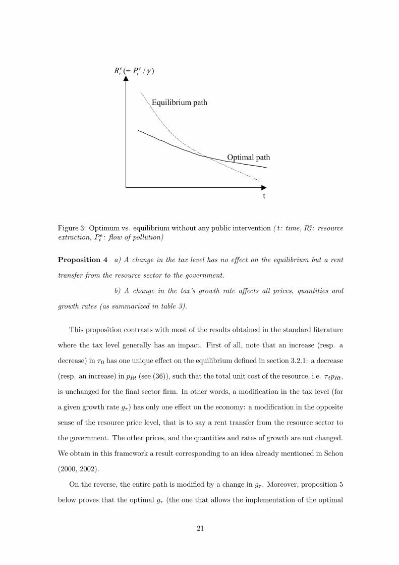
)/( γet
et PR =
Equilibrium path
Optimal path
t
Figure 3: Optimum vs. equilibrium without any public intervention ( t : time, Ret : resourceextraction, P et : flow of pollution)
Proposition 4 a) A change in the tax level has no effect on the equilibrium but a rent
transfer from the resource sector to the government.
b) A change in the tax’s growth rate affects all prices, quantities and
growth rates (as summarized in table 3).
This proposition contrasts with most of the results obtained in the standard literature
where the tax level generally has an impact. First of all, note that an increase (resp. a
decrease) in τ0 has one unique effect on the equilibrium defined in section 3.2.1: a decrease
(resp. an increase) in pRt (see (36)), such that the total unit cost of the resource, i.e. τ tpRt,
is unchanged for the final sector firm. In other words, a modification in the tax level (for
a given growth rate gτ ) has only one effect on the economy: a modification in the opposite
sense of the resource price level, that is to say a rent transfer from the resource sector to
the government. The other prices, and the quantities and rates of growth are not changed.
We obtain in this framework a result corresponding to an idea already mentioned in Schou
(2000, 2002).
On the reverse, the entire path is modified by a change in gτ . Moreover, proposition 5
below proves that the optimal gτ (the one that allows the implementation of the optimal
21

path) is negative. So, let us first consider a constant τ , and then start to increase it during
the first times and decrease it during future times: gτ becomes negative. Using equations
(30)-(34), we obtain the results summarized in table 3.
ξ = LeRD ξ = geA ξ = geR ξ = geY ξ = r
∂ξ
∂gτ> 0 > 0 < 0 < 0 < 0
if ε > 1 if ε > 1
Table 3: Effects of the environmental policy
First of all, note that the price ratio τ tpRt/wt is a decreasing function of gτ (see (36)
and (35)). Thus at steady-state, the lower gτ is, the higher τ tpRt (the price paid by the
firm for the resource) is relative to the wage. For this reason the firm producing the
homogeneous good will use more labour: LY increases.
Moreover, at steady-state, gτ tpRt/wt is equal to gτ + gpR − gw. Thus, equations (27)and (35) allow us to write gτ tpRt/wt = gτ + r − geY , which is an increasing function of gτ .Thus whereas a lower gτ makes the resource price higher relative to the wage, this effect
diminishes along time. Hence the firm will choose to buy less resource today and more
tomorrow relative to the path it chose with the initial gτ (see Figure 4): geR increases,.the
resource is extracted at a lower path.as it is shown in Table 3.
4.3 Implementation of the optimum
Proposition 5 If gτ = −(•
UPh0−ρUPh0UCFR
), which is equal to −δνω(ε−1)+ρ(ε+ω)ε+ω(1−α+αε) in the specified
case at the steady-state, then the equilibrium path is optimal.
Note that the optimal gτ is negative, which means that along the equilibrium growth
path, as the use of the resource decreases (geR is negative), the tax level decreases also.
Proof. We are searching gτ such as (8) and (9) are equivalent to (28) and (29). Clearly,
(8) and (28) are identical, and if gτ = −(•
UPh0−ρUP h0UCFR
), then (9) and (29) are identical also.
In the specified case, simple computations allow us to find gτ .such that LeRD (see (30))
and LoRD (see (14)) be equal.
22

)/( γet
et PR =
t
Figure 4: Impact of the environmental policy consisting in a decrease in gτ ( t: time, Ret :resource extraction, P et : flow of pollution)
5 Conclusion
In this paper we considered the following problem: how are the standard results of non-
renewable resources (growth) theory modified when we take into account the presence of
polluting emissions arising from the use of those resources?
Firstly, we were able to characterize optimality conditions in a very general manner
(that is, without specifying functional forms) since we avoided the technical complexity
inherent to certain hypothesis of the standard endogenous growth models. We thus defined
a Hotelling rule that was modified in two senses: on one hand, it is no longer strictly an
efficiency condition. Since pollution affects households’ preferences, these are accounted for
in the new Hotelling rule. On the other hand, it is now the accumulation of intellectual
capital (knowledge), instead of the accumulation of physical capital, which delays the
depletion of the resource.
Next, we studied the steady-state’s optimal paths and we described their properties.
Namely, we found once more that increases in households’ impatience (or in the egoism
of present generations), or in their preference for environmental quality, result in a slower
extraction of the resource.
23

We went on to present a decentralization of the economy, such that pollution is the
source of the model’s only distortion. There, the violation of the Hotelling rule at the
market equilibrium -when no environmental policy has been applied- is clearly identified.
Agents fail to incorporate the negative externality caused by the use of the resource: there
is no market for pollution. We also characterized the steady-state’s equilibrium path and
showed that the growth rate at which the resource is extracted is under-optimal: the
resource is depleted too rapidly. Moreover, contrarily to that observed at the optimum, an
increase in households’ impatience makes the economy deplete the resource even faster.
Finally, the fact that there is only one distortion in the model allows us to implement
a simple economic policy: a unit tax on the demand for the resource. We then showed
that, contrary to what is found in a large part of the literature, a change in the tax
level at the steady-state has no effect on the real variables of the economy and does not
allow us to correct the equilibrium path (in order to make it optimal). Indeed, such a
policy only entails a rent transfer from the enterprise that extracts the resource to the
government (who levies the tax). Conversely, a change in the tax’s growth rate affects all
prices, quantities and growth rates. We calculate the exact level of the latter growth rate
(negative) which sends the appropriate signal to markets and for which the optimum is
attained at equilibrium.
Certain elements -such as considering pollution as a stock and not a flow- could cer-
tainly add to our results. Moreover, including in our problem the possibility of substituting
the polluting non-renewable resource with a non-polluting but less productive renewable
resource (such as solar energy or hydrogen fuel cells) remains a very interesting line of
future research.
24

Appendix
A. Non specified optimality conditions
The current value Hamiltonian of the social planner’s program is
H = U [F (1− LRDt, At, Rt), h(Rt)] + µtq(At, LRDt)− νtRt.
where µt and νt are the costate variables.
The first order conditions ∂H/∂LRDt = 0 and ∂H/∂Rt = 0 yield
µt =UCFLqL
(40)
νt = UCFR + UPh0. (41)
Moreover, ∂H/∂At = ρµt − µt and ∂H/∂St = ρνt − νt yield
µtµt= ρ− FAqL
FL− qA (42)
andνtνt= ρ. (43)
Differentiating (40) with respect to time, we have
µtµt=UCCC + UCP P
UC+FLFL− qLqL. (44)
(44), together with (42) gives
ρ− UCCC + UCP PUC
=FLFL− qLqL+FAqLFL
+ qA, (45)
25
that is, the Ramsey-Keynes condition.
Differentiating (41) with respect to time, we have
νtνt=UCFR(
UCC C+UCP PUC
+ FRFR) + UPh
0(UPCC+UPP PUP+
.
h0h0 )
UCFR + UPh0. (46)
(46) together with (43) gives
ρ− UCCC + UCP PUC
=FRFR
+UPh
0
UCFR(UPCC + UPP P
UP+
.
h0
h0− ρ). (47)
Plugging (45) into (47) yields:
FLFL− qLqL+FAqLFL
+ qA =FRFR
+UPh
0
UCFR(UPCC + UPP P
UP+
.
h0
h0− ρ),
where UPh0
UCFR(UPCC+UPP PUP
+.
h0h0 − ρ) = UPh
0UCFR
(•UPh
0+•h0UP
UPh0 − ρ) = UPh0
UCFR(
•UPh
0UPh0 − ρ).
One gets finally
FLFL− qLqL+FAqLFL
+ qA =FRFR
+ (
•UPh
0 − ρUPh0
UCFR), (48)
that is the Hotelling condition.
B. Transversality conditions at the steady-state optimum
The first transversality condition is limt→+∞µtA
ote−ρt = 0, which is equivalent to
limt→+∞µ0e
gµtAo0egoAte−ρt = 0 at the steady state. Moreover, with the specifications
presented in section 2.3.1. within in the main text, equation (42) in Appendix A gives us
gµ = ρ− δνα + δLoRD(
ν−αα ). Thus we can see that gµ+ goA−ρ is negative if and only if LoRD
is lower than one.
The second transversality condition is limt→+∞νtS
ot e−ρt = 0, which is equivalent to
limt→+∞ν0e
gνtSo0egoSte−ρt = 0 at the steady-state. Equation (43) in Appendix A allows us to
find that gν + goS − ρ is negative if and only if goS(= goR) is negative.
26

References
Aghion, P. and P. Howitt, 1992, A Model of Growth Through Creative Destruction,
Econometrica 60, 323—351.
Aghion, P. and P. Howitt, 1998, Endogenous Growth Theory (The MIT Press).
Arrow, K.J., 1962, The Economic Implications of Learning-by-Doing, Review of Eco-
nomic Studies, 29(1), 155-173.
Barbier, E.B., 1999, Endogenous Growth and Natural Resource Scarcity, Environmen-
tal and Resource Economics, 14, 51—74.
Dasgupta, P.S. and G.M. Heal, 1979, Economic Theory and Exhaustible Resources,
UK (Oxford University Press).
Dasgupta, P.S., K.G. Mäler, G.B. Navaretti and D. Siniscalo, 1996, On Institutions
that Produce and Dissipate Knowledge, Mimeo.
Garg, P.C. and J.L. Sweeney, 1978, Optimal Growth with Depletable Resources, Re-
sources and Energy 1, 43—56.
Gradus, R. and S. Smulders, 1993, The Trade-off between Environmental Care and
Long-term Growth; pollution in three proto-type growth models, Journal of Economics,
58, 25-51.
Grimaud, A. and L. Rouge, 2003, Non-Renewable Resources and Growth with Vertical
Innovations: Optimum, Equilibrium and Economic Policies, Journal of Environmental
Economics and Management, 45, 433-453.
Grossman, G. and E. Helpman, 1991, Innovation and Growth in the Global Economy,
Cambridge MA (MIT Press).
Hotelling, H., 1931, The Economics of Exhaustible Resources, Journal of Political
Economy, 39, 137—175.
Jones, C.I., 2001, Population and Ideas: a Theory of Endogenous Growth, U.C. Berke-
ley mimeo.
Kolstad, C.D. and J.A. Krautkraemer, 1993, Natural Resource Use and the Environ-
ment, in: A.V. Kneese and J.L. Sweeney, eds., Handbook of Natural Resources and Energy
Economics, vol. III (Elsevier Science Publishers), 1219-1265.
27

Romer, P., 1990, Endogenous Technological Change, Journal of Political Economy, 98,
71—102.
Scholz, C.M. and G. Ziemes, 1999, Exhaustible Resources, Monopolistic Competition
and Endogeneous Growth, Environmental and Resource Economics, 13, 169—185.
Schou, P., 1996, A Growth Model with Technological Progress and Non-renewable
Resources, Mimeo, University of Copenhagen.
Schou, P., 2000, Polluting Non-Renewable Resources and Growth, Environmental and
Resource Economics, 16, 211-227.
Schou, P., 2002, When Environmental Policy is Superfluous: Growth and Polluting
Resources, Mimeo, University of Copenhagen.
Scotchmer, S., 1991, Standing on the Shoulders of Giants: Cumulative Research and
the Patent Law, Journal of Economic Perspective, Symposium on Intellectual Property
Rights.
Scotchmer, S., 1999, Cumulative Innovations in Theory and Practice, Working Paper,
U.C. Berkeley.
Stiglitz, J., 1974, Growth with Exhaustible Natural Resources : I) Efficient and Opti-
mal Growth, II) The Competitive Economy, Review of Economic Studies Symposium, 41,
123—152.
Tahvonen, O., 1997, Fossil Fuels, Stock Externalities, and Backstop Technology, Cana-
dian Journal of Economics, XXX, 855-874.
Tahvonen, O. and S. Salo, 2001, Economic Growth and Transition between Renewable
and Nonrenewable Energy Resources, European Economic Review, 45, 1379-1398.
Withagen, C., 1999, Optimal Extraction of Non-Renewable Resources, in J.C.J.M. van
den Bergh (ed), Handbook of Environmental and Resource Economics, Edward Elgar, 49-
58.
28

ξ = δ ξ = ε ξ = ρ ξ = ν ξ = ω
∂LoRD∂ξ
> 0 < 0 < 0 > 0 < 0
GR GR GR
∂goA∂ξ
> 0 < 0 < 0 > 0 < 0
GR GR GR
∂goR∂ξ
< 0 < 0 > 0 < 0 > 0
S,GR S,GR
∂goY∂ξ
> 0 < 0 < 0 > 0 > 0
S,GR S,GR S,GR
Table 1: Properties of the optimal path
29

ξ = δ ξ = ε ξ = ρ ξ = ν ξ = ω
∂LeRD∂ξ
> 0 < 0 < 0 > 0 = 0
GR GR GR
∂geA∂ξ
> 0 < 0 < 0 > 0 = 0
GR GR GR
∂geR∂ξ
< 0 < 0 < 0 < 0 = 0
if ε > 1 if geY > 0 if ε > 1
GR GR GR
∂geY∂ξ
> 0 < 0 < 0 > 0 = 0
if geY > 0
GR GR GR
Table 2: Properties of the equilibrium path
30

ξ = LeRD ξ = geA ξ = geR ξ = geY ξ = r
∂ξ
∂gτ> 0 > 0 < 0 < 0 < 0
if ε > 1 if ε > 1
Table 3: Effects of the environmental policy
31