pollution, electricity consumption, and income in the
TRANSCRIPT
Pollution, Electricity Consumption, and Income in the Context of Trade Openness in Zambia
Lackson Daniel Mudenda
Spring Semester 2016
Master Level, 30 ECTS
MSc Economics Program
ii
Abstract
This paper examines the Environmental Kuznets Curve (EKC) hypothesis and tests for
causality using Dynamic Ordinary Least Squares (DOLS) and the Vector Error Correction
Model (VECM). There is evidence of long-run relationships in the three models under
consideration. The Dynamic Ordinary Least Squares (DOLS) finds no evidence to support the
existence of an environmental Kuznets curve (EKC) hypothesis for Zambia in the long-run.
The evidence from the long-run suggests an opposite of the Environmental Kuznets Curve
(EKC), in that the results indicate a U-shaped curve relationship between income and carbon
emission. The conclusion on causality based on the VECM is that there is evidence of
neutrality hypothesis between either total electricity and income or between industrial
electricity and income in the short-run Additionally, there is evidence of conservation
hypothesis in the context of residential and agricultural electricity consumption.
Keywords: Dynamic OLS, Vector Error Correction Model, real GDP, CO2 Emissions,
Electricity consumption and Foreign Trade

iii
Acknowledgement
I thank God for everything. I thank my family for the unwavering support they have
continuously shown me during my studies. Specifically, I thank my sweetheart, Michelo for
the loving, caring and understanding attitude towards my studies. All the gratitude goes to my
mum who always encourages me to follow my gut and dreams. Many times it was hard for me,
but the people behind the force of encouragement kept pushing me.
I am sincerely grateful to my supervisor, Professor Runar Brännlund for the incessant guidance
through the writing process. I learnt an invaluable lot during this process, and I will be forever
grateful. Special thanks also go to Dr Amin Karimu, my co-supervisor, for the unimaginable
support in the econometrics and the paper as a whole. It was fun to try the many different
models in estimating and finally we opted for the optimal result. Am very grateful.
This thesis is part of my research work at Umea University during my Master of Science
degree in Economics, big thanks to the Swedish government and the Swedish Institute
Scholarship. A fulfilling experience I will cherish for the rest of my life. A carry with me a part
of Sweden that will forever be tattooed on my heart.
iv
Contents Abstract ...................................................................................................................................................... ii Acknowledgement .................................................................................................................................... iii List of Figures ........................................................................................................................................... iv List of Tables ............................................................................................................................................ iv 1.0 Introduction ......................................................................................................................................... 1
1.1 Purpose of Research ........................................................................................................................ 2 1.2 Background ..................................................................................................................................... 3 1.2.1 The Power Sector In Zambia ........................................................................................................ 8
2.0 Literature Review ............................................................................................................................. 10 3.0 Methodology ..................................................................................................................................... 17
3.1 Theoretical Underpinnings ............................................................................................................ 17 3.2 Econometric Strategy .................................................................................................................... 22 3.3 Data and Variable Definitions ....................................................................................................... 27
4.0 Estimations, Analysis and Discussion of Results ............................................................................. 31 4.1 Data Characteristics ...................................................................................................................... 31 4.2 Long-Run Relationship ................................................................................................................. 33 4.3 Short-Run Relationship ................................................................................................................. 36 4.4 Diagnostic Tests ............................................................................................................................ 38
5.0 Policy Analysis and Conclusion ....................................................................................................... 40 5.2 Possible Areas for further research and Limitations ..................................................................... 41 References........................................................................................................................................... 42 Appendix A .......................................................................................................................................... 45 Appendix B .......................................................................................................................................... 47 Appendix C: ......................................................................................................................................... 50 Appendix D .......................................................................................................................................... 51
List of Figures Figure 1: Trends of Carbon Emissions, Income, Trade and Electricity Consumption ............................. 5
Figure 2: Total Electricity consumption and real GDP in Zambia (1971-2010) ...................................... 6
Figure 3: General Equilibrium Interpretation of EKC .............................................................................. 22
List of Tables Table 1: Zambia's electricity capacity ...................................................................................................... 8
Table 2 Summary of Previous Studies .................................................................................................... 16
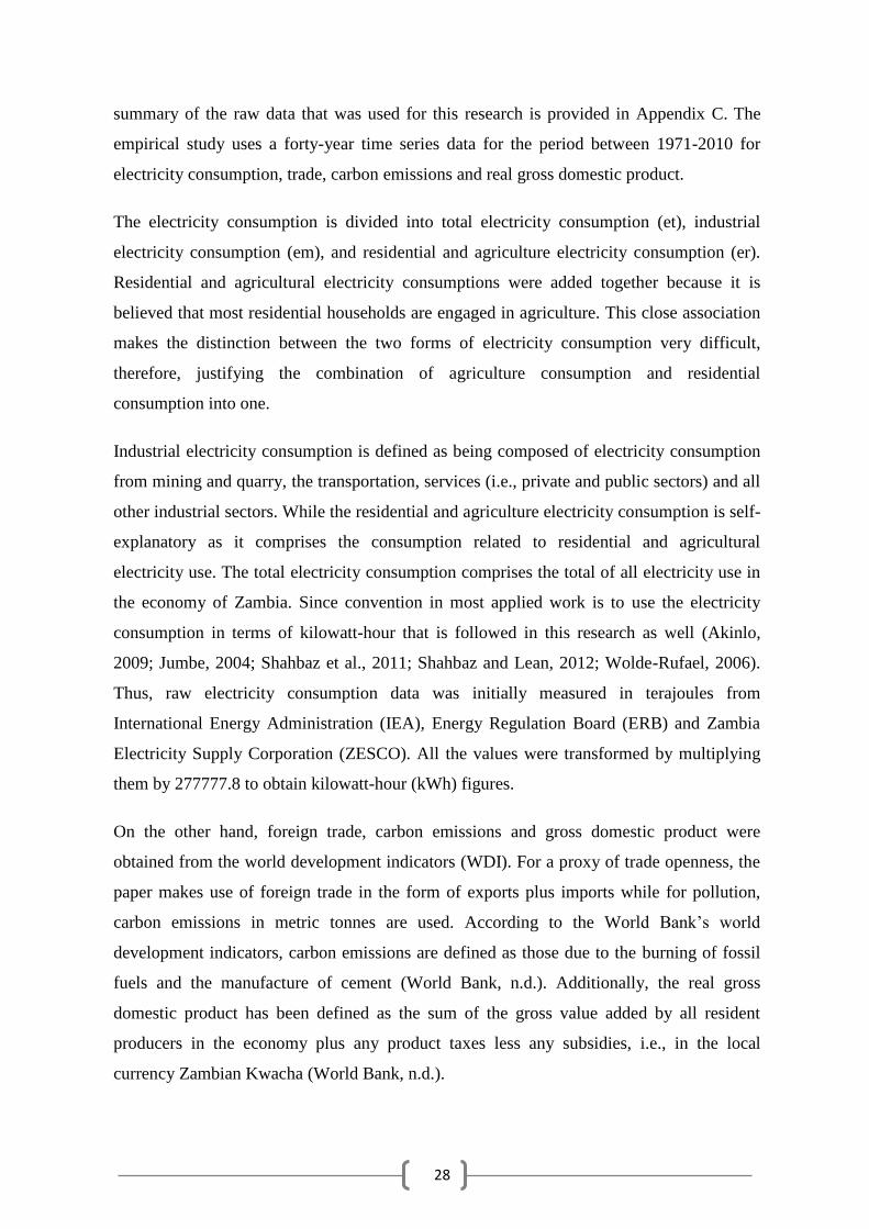
Table 3 Summary Statistics .................................................................................................................... 29
Table 4: Unit Root Test: Augmented Dickey-Fuller and Phillips-Perron .............................................. 31
Table 5 Lag Selection ............................................................................................................................. 32
Table 6 Cointegration Tests .................................................................................................................... 33
Table 7: Long-Run Equilibrium Relationship for the carbon equations ................................................. 34
Table 8: Short-Run Results for the carbon equation ............................................................................... 36
Table 9 Short-Run and Long-Run Granger Causality 𝜒2 Results .......................................................... 37
Table 10: VECM Model Diagnostic Tests.............................................................................................. 39
1
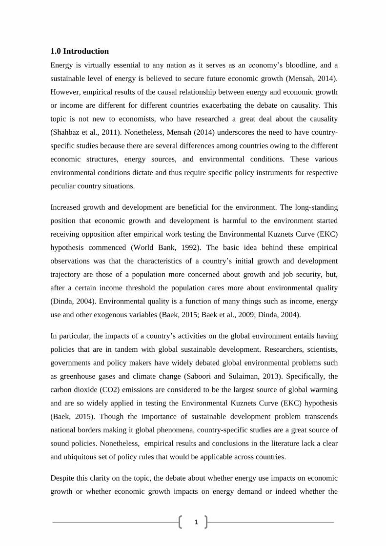
1.0 Introduction
Energy is virtually essential to any nation as it serves as an economy’s bloodline, and a
sustainable level of energy is believed to secure future economic growth (Mensah, 2014).
However, empirical results of the causal relationship between energy and economic growth
or income are different for different countries exacerbating the debate on causality. This
topic is not new to economists, who have researched a great deal about the causality
(Shahbaz et al., 2011). Nonetheless, Mensah (2014) underscores the need to have country-
specific studies because there are several differences among countries owing to the different
economic structures, energy sources, and environmental conditions. These various
environmental conditions dictate and thus require specific policy instruments for respective
peculiar country situations.
Increased growth and development are beneficial for the environment. The long-standing
position that economic growth and development is harmful to the environment started
receiving opposition after empirical work testing the Environmental Kuznets Curve (EKC)
hypothesis commenced (World Bank, 1992). The basic idea behind these empirical
observations was that the characteristics of a country’s initial growth and development
trajectory are those of a population more concerned about growth and job security, but,
after a certain income threshold the population cares more about environmental quality
(Dinda, 2004). Environmental quality is a function of many things such as income, energy
use and other exogenous variables (Baek, 2015; Baek et al., 2009; Dinda, 2004).
In particular, the impacts of a country’s activities on the global environment entails having
policies that are in tandem with global sustainable development. Researchers, scientists,
governments and policy makers have widely debated global environmental problems such
as greenhouse gases and climate change (Saboori and Sulaiman, 2013). Specifically, the
carbon dioxide (CO2) emissions are considered to be the largest source of global warming
and are so widely applied in testing the Environmental Kuznets Curve (EKC) hypothesis
(Baek, 2015). Though the importance of sustainable development problem transcends
national borders making it global phenomena, country-specific studies are a great source of
sound policies. Nonetheless, empirical results and conclusions in the literature lack a clear
and ubiquitous set of policy rules that would be applicable across countries.
Despite this clarity on the topic, the debate about whether energy use impacts on economic
growth or whether economic growth impacts on energy demand or indeed whether the
2
causality is both ways or non-existent, is far from over (Odhiambo, 2009). Additionally, the
dearth of literature on energy use, emissions, trade openness and economic growth for
African countries indicates that not many studies have devoted to this topic from the
African perspective (Baek, 2015; Wolde-Rufael, 2006). Therefore, the case of Zambia
provides yet, another exciting area of research because of the persistent imbalances between
electricity supply and electricity peak demand. This area of research for Zambia is also
highly motivated in the light of the famous Pollution Haven Hypothesis (PHH). The
hypothesis posits that poor economies tend to adopt weak environmental policies to attract
multinational investment in an attempt to ward off harsh international competitiveness
(Baek et al., 2009).
1.1 Purpose of Research
The general aim of this research is to test for the environmental Kuznets curve hypothesis
and to characterise the Granger causality between electricity consumption, emissions and
economic growth in Zambia between 1971 and 2010. Nonetheless, the specific objectives
are;
(i) To check the presence of the environmental Kuznets curve (EKC) hypothesis for
Zambia with a particular focus on carbon emissions.
(ii) To check the causality between sector-wise electricity consumption (i.e., total
electricity, industrial electricity, agricultural and residential electricity
consumptions), economic growth and carbon emissions in Zambia.
Therefore, in light of the above specific objectives the study investigates and provides
answers to the following research questions;
(i) Is there evidence of the environmental Kuznets curve (EKC) hypothesis for
Zambia?
(ii) Is there Granger causality between total electricity consumption, economic growth
and carbon emissions?
(iii) Is there Granger causality between sector-wise electricity consumption (i.e., total
electricity, industrial electricity, agricultural and residential electricity
consumptions), economic growth and carbon emissions?
This study is confined to studying Granger causality between electricity consumption (i.e.,
both aggregated and disaggregated) and economic growth in Zambia for the period between
1971-2010. The use of aggregated and disaggregated electricity here implies the application
3
electricity use from the different sectors, i.e., total electricity, industrial electricity and
agricultural and residential electricity consumption. Additionally, the Environmental
Kuznets Curve (EKC) hypothesis is tested for Zambia in line with the aggregated and
disaggregated electricity. This twin-strand based research on both environmental Kuznets
curve hypothesis and Granger causality between electricity consumption and income is
important for policy formulation.
Regarding policy, an understanding of the direction of causality and the examination of the
environmental Kuznets curve are critical for any economy. Policymakers with knowledge
of the direction of causality would institute appropriate and environmentally friendly
energy policies. For instance, the presence of the environmental Kuznets curve hypothesis
indicates that having a growth objective for the economy would prove beneficial in the
long-run. On the other hand, Granger causality between electricity consumption and income
could lead to either conservation, growth, bidirectional or neutrality hypotheses. The
presence of conservation hypothesis means that conservation policies may not adversely
affect economic growth while growth hypothesis implies that growth is energy dependent
and any energy disruptions would imply adverse effects on economic growth. Basically, the
knowledge would provide government policymakers with the necessary head start in policy
formulation.
1.2 Background
The topic of environmental degradation, economic growth, and energy use is polarised
between causality and testing of the environmental Kuznets curve. Firstly, the causality
relationship has been categorised into four (4) groups, the neutrality hypothesis, growth
hypothesis, conservative hypothesis, and bi-directional hypothesis (Ozturk, 2010). The
presence of neutrality hypothesis means that there is no causality while the bi-directional
hypothesis (or feedback hypothesis) suggests that a uni-directional causality is in both
directions between electricity consumption and income. On the other hand, growth
hypothesis says that economic growth is electricity consumption-led while the conservation
hypothesis implies that electricity consumption is growth-led (Bildirici, 2013; Ghosh, 2002;
Wolde-Rufael, 2006).
The direction of causality between electricity consumption and economic growth has
interesting policy implications for any economy. For instance, the presence of conservation
hypothesis means that conservation policies may not adversely affect growth. Examples of
4
conservation policies are the scrapping off of energy subsidies, the episodes of load-
shedding or daylight saving time may not adversely affect growth. Although, with load
shedding the disruptions are more about momentary effects as opposed to changes in
electricity use from year to year. On the other hand, the presence of growth hypothesis has
the policy implication that growth is energy dependent and any energy disruptions mean
adverse effects on economic growth and thereby affecting the standards of living of the
population (Kouakou, 2011; Odhiambo, 2009; Shiu and Lam, 2004;).
Secondly, the energy-growth-environment theme also concerns the investigation of the
environmental Kuznets curve (EKC) hypothesis. The theory claims that it cannot be ruled
out that higher incomes may change people's preferences which in turn affects government
policies, which in the end lowers emissions. This translates to the claim that by countries
becoming wealthy they would inevitably fight environmental degradation in the long-run.
However, according to Perman and Perma (2011), the validity of this proposition involves
investigation of two questions; Firstly, is the data consistent with the environmental
Kuznets curve (EKC) hypothesis? Secondly, if the Environmental Kuznets Curve (EKC)
hypothesis holds, does that mean the prospects of growth is great news for the
environment? Additionally, It has been argued that international trade is one of the most
important factors that can explain the Environmental Kuznets Curve (EKC) hypothesis
(Dinda, 2004; Kohler, 2013). Therefore, investigation of the carbon emissions, income, and
energy use is better served in the context of trade openness.
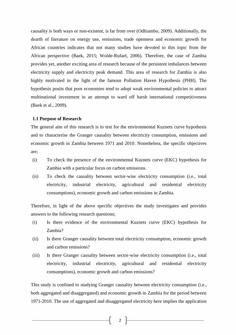
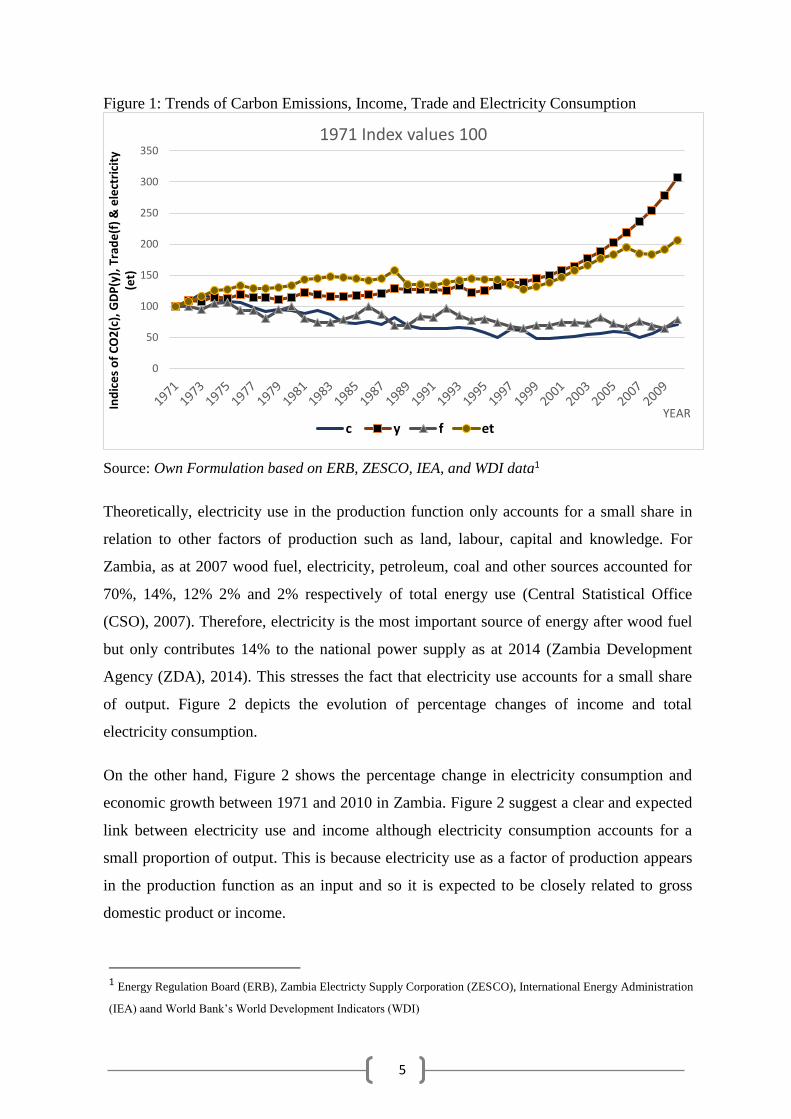
Figure 1 shows the trends of carbon emissions, income, foreign trade (i.e., exports plus
imports) and electricity consumption for Zambia for the period between 1971-2010 (i.e., all
in index form). Income or real gross domestic product and total electricity consumption rise
steadily from 1971 to 2010 with income growing more than the increase in total electricity
consumption. On the other hand, carbon emissions and foreign trade are relatively stable
over the same period. This raw data appears to suggest that the movements of electricity
consumption and income are more related to each other than with carbon emissions and
foreign trade. This provides a compelling motivation to check the econometric implication
of these supposed relationships. Figure 1 shows the evolution of variables over time.
5
Figure 1: Trends of Carbon Emissions, Income, Trade and Electricity Consumption
Source: Own Formulation based on ERB, ZESCO, IEA, and WDI data1
Theoretically, electricity use in the production function only accounts for a small share in
relation to other factors of production such as land, labour, capital and knowledge. For
Zambia, as at 2007 wood fuel, electricity, petroleum, coal and other sources accounted for
70%, 14%, 12% 2% and 2% respectively of total energy use (Central Statistical Office
(CSO), 2007). Therefore, electricity is the most important source of energy after wood fuel
but only contributes 14% to the national power supply as at 2014 (Zambia Development
Agency (ZDA), 2014). This stresses the fact that electricity use accounts for a small share
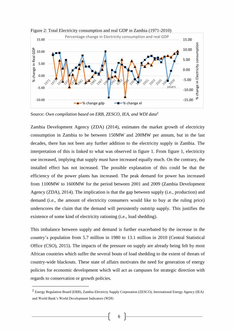
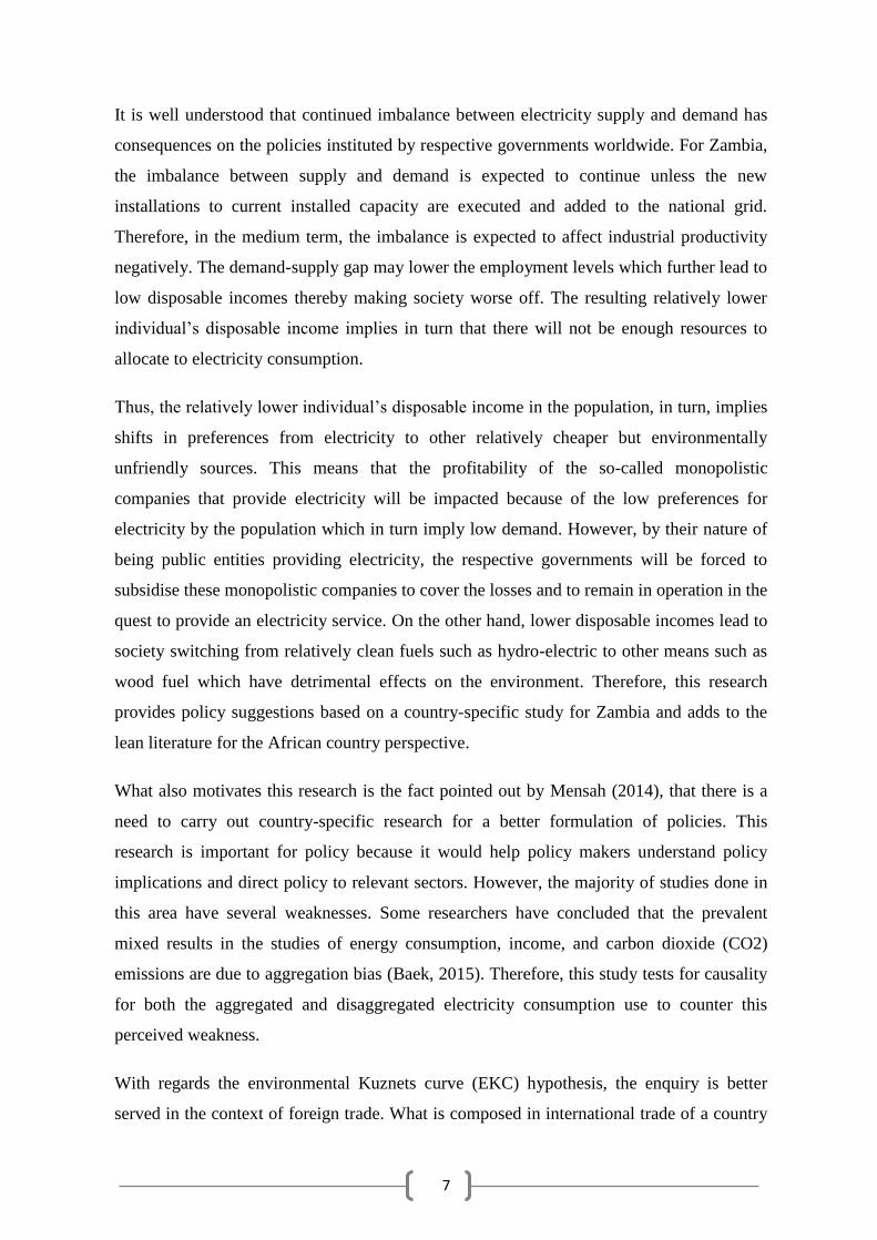
of output. Figure 2 depicts the evolution of percentage changes of income and total
electricity consumption.
On the other hand, Figure 2 shows the percentage change in electricity consumption and
economic growth between 1971 and 2010 in Zambia. Figure 2 suggest a clear and expected
link between electricity use and income although electricity consumption accounts for a
small proportion of output. This is because electricity use as a factor of production appears
in the production function as an input and so it is expected to be closely related to gross
domestic product or income.
1 Energy Regulation Board (ERB), Zambia Electricty Supply Corporation (ZESCO), International Energy Administration
(IEA) aand World Bank’s World Development Indicators (WDI)
0
50
100
150
200
250
300
350
Ind
ice
s o
f C
O2
(c),
GD
P(y
), T
rad
e(f
) &
ele
ctri
city
(e
t)
YEAR
1971 Index values 100
c y f et
6
Figure 2: Total Electricity consumption and real GDP in Zambia (1971-2010)
Source: Own compilation based on ERB, ZESCO, IEA, and WDI data2
Zambia Development Agency (ZDA) (2014), estimates the market growth of electricity
consumption in Zambia to be between 150MW and 200MW per annum, but in the last
decades, there has not been any further addition to the electricity supply in Zambia. The
interpretation of this is linked to what was observed in figure 1. From figure 1, electricity
use increased, implying that supply must have increased equally much. On the contrary, the
installed effect has not increased. The possible explanation of this could be that the
efficiency of the power plants has increased. The peak demand for power has increased
from 1100MW to 1600MW for the period between 2001 and 2009 (Zambia Development
Agency (ZDA), 2014). The implication is that the gap between supply (i.e., production) and
demand (i.e., the amount of electricity consumers would like to buy at the ruling price)
underscores the claim that the demand will persistently outstrip supply. This justifies the
existence of some kind of electricity rationing (i.e., load shedding).
This imbalance between supply and demand is further exacerbated by the increase in the
country’s population from 5.7 million in 1980 to 13.1 million in 2010 (Central Statistical
Office (CSO), 2015). The impacts of the pressure on supply are already being felt by most
African countries which suffer the several bouts of load shedding to the extent of threats of
country-wide blackouts. These state of affairs motivates the need for generation of energy
policies for economic development which will act as campuses for strategic direction with
regards to conservation or growth policies.
2 Energy Regulation Board (ERB), Zambia Electricty Supply Corporation (ZESCO), International Energy Agency (IEA)
and World Bank’s World Development Indicators (WDI)
-15.00
-10.00
-5.00
0.00
5.00
10.00
15.00
-10.00
-5.00
0.00
5.00
10.00
15.00
% c
han
ge in
Ele
ctri
city
co
nsu
mp
tio
n
% c
han
ge in
Rea
l GD
P
years
Percentage change in Electricity consumption and real GDP
% change gdp % change el
7
It is well understood that continued imbalance between electricity supply and demand has
consequences on the policies instituted by respective governments worldwide. For Zambia,
the imbalance between supply and demand is expected to continue unless the new
installations to current installed capacity are executed and added to the national grid.
Therefore, in the medium term, the imbalance is expected to affect industrial productivity
negatively. The demand-supply gap may lower the employment levels which further lead to
low disposable incomes thereby making society worse off. The resulting relatively lower
individual’s disposable income implies in turn that there will not be enough resources to
allocate to electricity consumption.
Thus, the relatively lower individual’s disposable income in the population, in turn, implies
shifts in preferences from electricity to other relatively cheaper but environmentally
unfriendly sources. This means that the profitability of the so-called monopolistic
companies that provide electricity will be impacted because of the low preferences for
electricity by the population which in turn imply low demand. However, by their nature of
being public entities providing electricity, the respective governments will be forced to
subsidise these monopolistic companies to cover the losses and to remain in operation in the
quest to provide an electricity service. On the other hand, lower disposable incomes lead to
society switching from relatively clean fuels such as hydro-electric to other means such as
wood fuel which have detrimental effects on the environment. Therefore, this research
provides policy suggestions based on a country-specific study for Zambia and adds to the
lean literature for the African country perspective.
What also motivates this research is the fact pointed out by Mensah (2014), that there is a
need to carry out country-specific research for a better formulation of policies. This
research is important for policy because it would help policy makers understand policy
implications and direct policy to relevant sectors. However, the majority of studies done in
this area have several weaknesses. Some researchers have concluded that the prevalent
mixed results in the studies of energy consumption, income, and carbon dioxide (CO2)
emissions are due to aggregation bias (Baek, 2015). Therefore, this study tests for causality
for both the aggregated and disaggregated electricity consumption use to counter this
perceived weakness.
With regards the environmental Kuznets curve (EKC) hypothesis, the enquiry is better
served in the context of foreign trade. What is composed in international trade of a country
8
reflects the energy consumption of that country and nations that export more manufactured
goods tend to use more energy (Dinda, 2004). In most cases, nations that export
manufactured goods are developed countries while poor and developing countries are often
net exporters of raw materials. However, when structural changes in production in
developed economies are not met by structural changes in consumption a mismatch in those
markets is created leading to industries being displaced to developing countries (Copeland
and Taylor, 1995). As a result, the argument is that developing countries mostly have weak
environmental policies thereby becoming victims of the said displacement hypothesis.
Therefore, environmental Kuznets curve (EKC) hypothesis essentially records displacement
of dirty industries to less developed economies (Copeland and Taylor, 1995). This explains
why developing countries like Zambia face the possibility of having pollution intensive
industries that are in fact only displaced from developed countries.
1.2.1 The Power Sector In Zambia
In Zambia, the electricity sector is considered by some as, at best being an oligopoly3
market with the presence of Lusemfwa Hydro Power company (LHPC), Ndola Energy
Company Limited and Zengamina Hydro Power Company (ZHPC) as Independent Power
Producers (IPP) (Energy Regulation Board (ERB), 2015). Others are Copperbelt Energy
Corporation (CEC) an independent transmission company, Northwestern Energy Company
Limited (NEC) and Kariba North Bank Power Extension Corporation Limited and finally,
Zambia Electricity Supply Corporation (ZESCO), the state-owned generation, transmission,
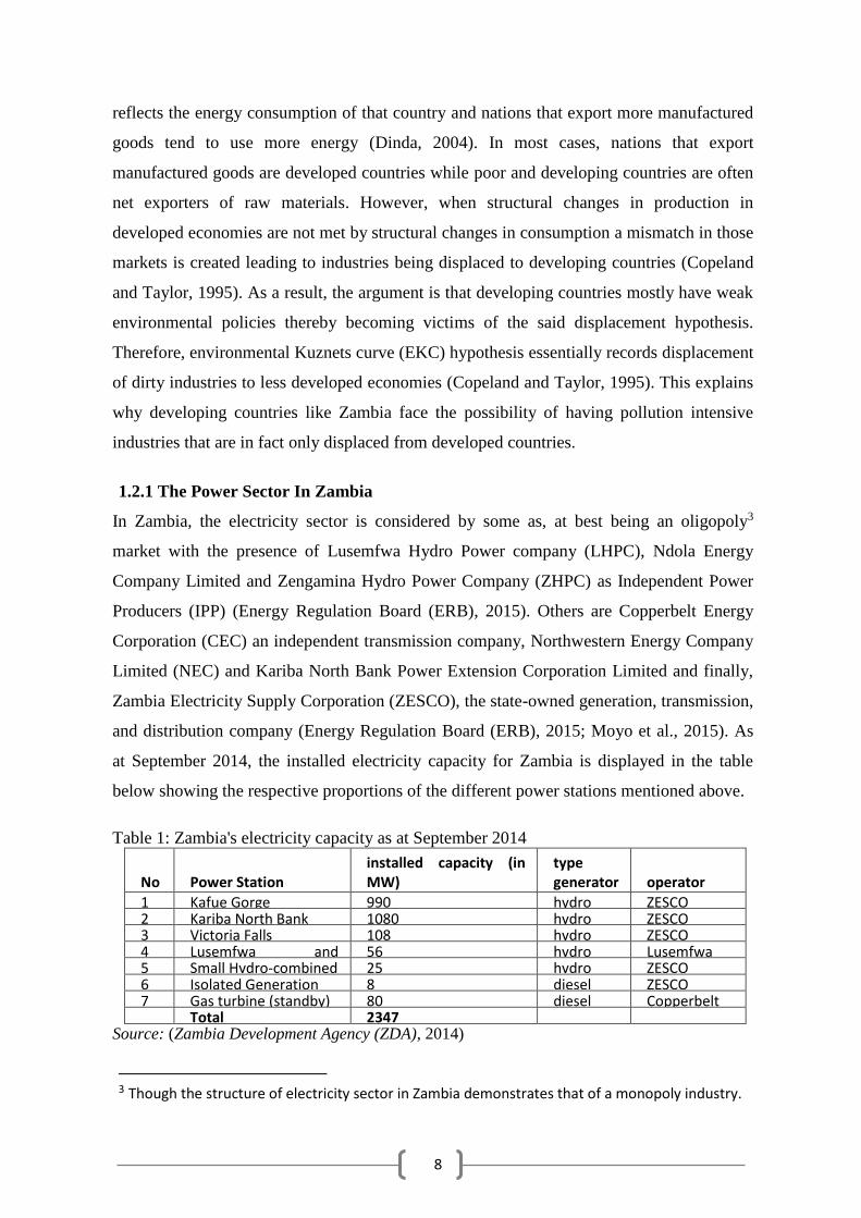
and distribution company (Energy Regulation Board (ERB), 2015; Moyo et al., 2015). As
at September 2014, the installed electricity capacity for Zambia is displayed in the table
below showing the respective proportions of the different power stations mentioned above.
Table 1: Zambia's electricity capacity as at September 2014
No Power Station installed capacity (in MW)
type generator operator
1 Kafue Gorge 990 hydro ZESCO 2 Kariba North Bank 1080 hydro ZESCO 3 Victoria Falls 108 hydro ZESCO 4 Lusemfwa and
Mulungushi 56 hydro Lusemfwa
Hydro 5 Small Hydro-combined 25 hydro ZESCO 6 Isolated Generation 8 diesel ZESCO 7 Gas turbine (standby) 80 diesel Copperbelt
Energy Corp Total 2347 Source: (Zambia Development Agency (ZDA), 2014)
3 Though the structure of electricity sector in Zambia demonstrates that of a monopoly industry.
9
Most countries underwent different forms of reforms because of both external and internal
shocks in Africa, and the successes of these reforms remain unclear (Mensah, 2014).
Nonetheless, electricity sector reform has been a success in other parts of the world such as
the UK, Nordic countries, Argentina, Chile, USA (Texas), parts of Australia and elsewhere,
though what is still prevalent in many countries is unsatisfactory and incomplete reform
(Joskow, 2008). For Zambia, Vagliasindi and Besant-Jones (2013) state that the country’s
case is a case study of difficulties with power sector reform process due to hard economic
conditions and a lack of a sustained political will.
The power sector in Zambia is still highly integrated. This means that one company, the
Zambia Electricity Supply Corporation (ZESCO) still has the monopoly power as it
handles generation, as well as transmission and distribution. The other privately owned
companies manage the transmission and distribution. However, in the past few decades, the
Zambian government has tried to improve the current state of the electricity supply through
economic and power sector reforms. For instance, in 1994, the Zambian Government
formulated a national energy policy (NEP) whose primary objective is “to promote
optimum supply and utilisation of energy, especially indigenous forms, to facilitate the
socio-economic development of the country and maintenance of a safe and healthy
environment” (World Bank, 2002). There are several arguments for and against power
sector reforms, but what matters are the effects of intended objectives. This attests to the
fact that the Republic of Zambia has tried to resolve the supply-demand imbalance.
The rest of this paper is organised as follows. The next section discusses the literature
review. The methodology employed and the data utilised in the study are discussed in
section three (3). The empirical results, analysis and discussion, are presented in Section
four (4). Finally, conclusions and policy recommendations of the study are presented in
Section Five (5).
10
2.0 Literature Review
The literature on carbon emissions, economic growth, and energy consumption is polarised
between the Environmental Kuznets Curve (EKC) hypothesis and the relationship between
the economic growth and energy use (Saboori and Sulaiman, 2013). In this vein, this paper
follows that convention by discussing previous empirical studies using a two strand
approach, firstly by exploring previous literature on the growth-energy nexus and then
moving onto the review of the Environmental Kuznets Curve (EKC) Hypothesis in the
context of trade openness.
As alluded to, there is abundant literature on the theme of electricity consumption and
economic growth with varying and conflicting results. Most studies in this area focus on
examining the roles of energy in stimulating economic growth and determining the
causality between electricity consumption and economic growth (Ozturk, 2010). It is
concluded that there is no consensus on the results of these two objectives in the literature,
and therefore, no policy recommendations can be applied across countries. The
contemporary literature on energy consumption and economic activity indicates that there
are four (4) outcomes of the said causal relationship in the form of neutrality hypothesis,
growth hypothesis, conservative hypothesis, and bi-directional hypothesis.
Additionally, within the four (4) categories above there two (2) more classifications with
the first being focussed on country-specific studies while the other on multi-country studies
(Shahbaz et al., 2011). Initial studies on this subject go as far back as the second half of the
20th century with a seminal paper by Kraft and Kraft (1978) for the United States of
America (USA), on which subsequent studies are based albeit with varying methodologies,
sample sizes, and countries (Ozturk, 2010). Early studies were characterised by mixed
results, an outcome that is still prevalent in more recent studies as well.
Firstly, some studies have found evidence for the conservation hypothesis in which there is
uni-directional causality running from economic growth to energy consumption without any
feedback. Recently, Ghosh (2002) investigated causality between electricity consumption
and economic growth in India and found the existence conservation hypothesis. That result
in the study is coherently explained to imply that with increases in growth, the population
tends to have more disposable income and therefore consumes more and more electricity.
The dependency on electricity was understood to be from the greater use of electric gadgets
in the agriculture sector and the inter-fuel substitution from conventional fuels like coal,
11
firewood, and oil in various areas. The conservation hypothesis found by Ghosh, (2002)
implies that conservation policies such as rationing, the tariff structure policies, electricity
efficiency improvement, and demand side management can be done without affecting the
economic growth of India.
In a different light, Wolde-Rufael (2006) investigated the long-run and causality
relationship between electricity consumption per capita and real domestic product per
capita for Seventeen (17) African countries, including Zambia. Wolde-Rufael (2006)
applied the cointegration test and modified causality test due to Pesaran et al. (2001) and
Toda and Yamamato (1995) respectively. The study found a long-run cointegrating
relationship for nine (9) of the countries while causality for twelve (12) countries though
the investigation did not offer a definite stance on the existence or non-existence of a causal
relationship between electricity consumption and economic growth. Moreover, their
findings are to be taken with care as the electricity consumption variable used accounts for
a small share of total energy and is confined to urban, commercial and industrial sectors
Wolde-Rufael, (2006). With regards to Zambia, Wolde-Rufael, (2006) found a positive
unidirectional causality running from GDP per capita to electricity consumption per capita
implying that increase in economic growth causes the rise in electricity consumption.
The conservation hypothesis result for Zambia found by Wolde-Rufael (2006) is in line
with the findings of a similar and recent study of Bildirici (2013). Bildirici (2013),
however, applied the Autoregressive Distributed Lag (ARDL) approach and Vector Error
Correction Models (VECM) on fewer countries and confirmed the result found by Wolde-
Rufael (2006). Therefore, previous results that have included Zambia in their samples have
found that Zambia could undertake conservation policies without affecting the growth of
the Economy.
Secondly, other studies have on the other hand found the existence of the Growth
Hypothesis in which an economy’s growth is dependent on electricity consumption. For
instance, Shiu and Lam (2004) found growth hypothesis for China, the second largest
consumer of electricity in the world. By applying the error correction model, Shiu and Lam
(2004) found a unidirectional causality running from electricity consumption to economic
growth, though the rate of growth of electricity was not found to be a direct one-to-one
correlation with economic growth. That conclusion means that restrictions on energy use in
China may adversely affect growth while the increase in energy consumption may
12
contribute to economic growth. The finding further indicates that energy consumption plays
a vital role in economic growth both directly and indirectly in the production process as a
complement to labour and capital (Ozturk, 2010).
Using a similar approach, Akinlo (2009) found growth hypothesis in the investigation of the
electricity and growth relationship for Nigeria for the period between 1980 and 2006. That
is, the causality result was a unidirectional causal relationship running from electricity
consumption to economic growth without feedback for both the short-run and long-run
Akinlo (2009). As expected, the implication is that Nigeria is highly dependent on energy
because any disruptions in Energy affects growth, based on this study. Besides the usual
cointegration and error correction model approach in this study, the Hodrix-Prescott (HP)
filter was applied so as to get a stronger result than mere cointegration (Akinlo, 2009). This
was done so as to decompose the trend, and cyclical components and the result showed that
electricity consumption is a cause of cyclical fluctuation or business cycles (Akinlo, 2009).
One of the criticisms of the study by Akinlo (2009) was the application of the bivariate
model which would suffer from omitted variable bias, and this prompted Akpan and Akpan
(2012) to add emission as a third variable to the investigation.
Thirdly, causality literature of electricity consumption and economic growth has also
indicated that some studies had found a bi-directional causality relationship. In this vein, by
noting the limitations of bivariate studies, Odhiambo (2009) conducted a trivariate study on
electricity consumption and economic growth for South Africa (i.e., between 1971-2006)
by incorporating a rate of unemployment in the bivariate framework. The study found
bidirectional causality between electricity consumption and economic growth irrespective
of whether in the short-run or long-run, implying that the two complement each other
(Odhiambo, 2009). The bidirectional study means that energy use and economic growth
complement each other.
In a similar fashion, Shahbaz et al. (2011) investigated causality between economic growth,
employment and electricity consumption using Granger causality and the Vector Error
Correction Model (VECM) and found a bi-directional causal relationship for Portugal in the
long-run. However, in the short-run, it was concluded that there is a unidirectional causal
relationship running from economic growth to electricity consumption without feedbacks.
The implication of these findings by Shahbaz et al. (2011) is that policies should take into
account both short-run and long-run results and their impact. For instance, the conservation
13
hypothesis in the short run implies that policies such as daylight saving time, load shedding,
demand side managements and rationing are only appropriate in the short-run but would
affect growth in the long-run.
On the other hand, Kouakou (2011) used an Autoregressive Distributed Lag (ARDL)
approach to cointegration and the Error Correction Model (ECM) for three variables (i.e.,
electricity consumption, Industry value added and GDP) for Cote d’Ivoire. Kouakou (2011)
found a bi-directional causality relationship only in the short-run while in the long-run, only
a growth hypothesis was evident. The policy implications in the short-run for Cote d’Ivoire
are that energy consumption and economic growth complement each other while in the
long-run growth is energy dependent and disruptions in energy, in the long-run, would
affect long-run growth.
Using different versions of Gross Domestic Product (GDP), Jumbe (2004) investigated the
causality question for Malawi (i.e., 1970-1999) and applied both the standard Granger
causality (GC) Test and the Error Correction Model (ECM). Jumbe (2004) contrasted the
causality relationship between electricity consumption and overall Gross Domestic Product
(GDP); electricity consumption and agricultural-GDP; and electricity consumption and
non-agricultural-GDP. A bi-directional causality between Gross Domestic Product (GDP)
and electricity consumption was found using Granger causality tests while a uni-directional
causality was found using the ECM approach. However, the two methods found a uni-
directional causality running from non-agriculture GDP to electricity consumption.
Fourthly, the literature on the causality between electricity consumption and economic
growth has also indicated that some studies do not find a causal relationship. For instance,
Akpan and Akpan (2012) uses the multivariate Vector Error Correction model (VECM) as
an improvement of the bivariate study by Akinlo (2009) for Nigeria. The inclusion of a
third variable in the study changed the Growth Hypothesis result found by Akinlo (2009).
Akpan and Akpan (2012) finds evidence of the absence of causality in the relationship
implying the presence of the neutrality hypothesis for Nigeria. Therefore, the conclusion
was that there is no causality relationship between the energy use and economic growth.
On the other hand, most other literature also focusses on testing the Environmental Kuznets
Curve (EKC) hypothesis both for individual countries and also for multi-country studies. A
summary of a review of previous studies on the Environmental Kuznets Curve (EKC)
14
hypothesis is provided by Dinda (2004). Some studies have supported the Environmental
Kuznets Curve (EKC) hypothesis while others do not support the hypothesis. Additionally,
Some empirical studies that have incorporated trade openness in the investigation of
electricity consumption, economic growth, and emissions have found pro-environmental
results while others indicate that trade is harmful to the environment (Kohler, 2013).
Kohler (2013) investigates this for South Africa using Vector Autoregressive (VAR) model
and finds a long-run relationship between environmental quality, energy consumption, and
foreign trade. Kohler (2013) applied the Vector Autoregressive (VAR) model to test the
precise relationship between growth and emissions or the Environmental Kuznets Curve
(EKC) hypothesis. It was found to be hard to characterise the Environmental Kuznets Curve
(EKC) hypothesis in the presence of foreign trade. However, the presence of foreign trade
was surprisingly found to be beneficial for South Africa’s environment.
In contrast, Saboori and Sulaiman (2013) applied the Vector Error Correction Model
(VECM), Autoregressive Distributed Lag (ARDL) model and the Johansen-Juselius
maximum likelihood approach to check for cointegration for Malaysia. Saboori and
Sulaiman (2013) found bi-directional causality between economic growth and carbon
emission with disaggregated energy sources (i.e., coal, oil, gas, and electricity) meaning
that energy and growth complement each other. Saboori and Sulaiman (2013) ascertained
the presence of the Environmental Kuznets Curve (EKC) hypothesis for Malaysia (i.e.,
1980-2013) for disaggregated energy sources (coal, oil, gas, and electricity). However, the
Environmental Kuznets Curve (EKC) hypothesis was found absent for aggregate Energy
use. However, using data for the period between 1971 and 2003, Chandran et al. (2010)
also applied an ARDL approach for Malaysia but with the application of both a bivariate
and multivariate setting. In contrast, this paper found evidence of the growth hypothesis in
which there is a unidirectional causality running from electricity consumption to economic
growth.
Similarly, using an Autoregressive Distributed Lag (ARDL) approach, Baek (2015)
investigates the Environmental Kuznets Curve (EKC) hypothesis for Arctic countries. The
study for the Arctic countries found little evidence of Environmental Kuznets Curve (EKC)
hypothesis with only Iceland of the eight (8) confirming the hypothesis.Alkhathlan and
Javid (2013) used the same approach as Saboori and Sulaiman (2013) but for Saudi Arabia
and obtained slightly different results. Alkhathlan and Javid (2013) used the autoregressive
15
distributed lag model on both aggregated and disaggregated data on energy consumption.
No evidence of the environmental Kuznets curve is found in their study, and with regards to
causality (i.e., between energy and economic growth) none is found in the short-run.
However, in the long-run, there is evidence of the growth hypothesis for Saudi Arabia.
Additionally, Ouédraogo (2010) and Shahbaz and Lean (2012) also applied the
autoregressive distributed lag model using data for Pakistan and Burkina Faso. The two
studies also found evidence of a bidirectional causality between electricity consumption and
economic growth for the respective countries.
Baek et al. (2009) also used the Johansen Cointegration Approach and Cointegrated Vector
Autoregressive (CVAR) model to examine the dynamic impact of trade on the environment
using a time series dataset of Sulphur emissions (SO2), trade and income for 50 countries
for the period 1960-2000. Baek et al., (2009) found a bidirectional causality running from
trade/Income to emissions for developed countries while for developed countries a
bidirectional causality running from Sulphur emissions to trade/Income. This means that the
Environmental Kuznets Curve (EKC) hypothesis and Pollution Haven Hypothesis was
confirmed for developed countries and developing countries respectively.
In a nutshell, the literature reviewed in this paper indicates that the causality between
electricity consumption and economic growth can result in conservation hypothesis
(Bildirici, 2013; Wolde-Rufael, 2006), growth hypothesis (Akinlo, 2009; Shiu and Lam,
2004), or bi-directional causality (Jumbe, 2004; Kouakou, 2011; Odhiambo, 2009;
Shahbaz et al., 2011). However, some studies have, in fact, found no causality (Akpan and
Akpan, 2012). This conclusion indicates that there is a mixed result of previous studies on
the relationship between electricity consumption and economic growth. Therefore, from the
current body of literature, each study produces policy recommendations unique to
respective countries, thereby corroborating the importance of country-specific research on
this subject. It is clear that the previous studies concentrate more on the aggregate
electricity consumption without considering the country-specific-industry causality.
Additionally, the literature points to the fact that studies that have included Zambia in their
samples (Bildirici, 2013; Wolde-Rufael, 2006) have found the presence of the conservation
hypothesis.
With regards environmental degradation, some studies have found evidence of the
Environmental Kuznets Curve (EKC) hypothesis while others have not. As far as this study
16
is concerned, no research has investigated the Environmental Kuznets Curve (EKC)
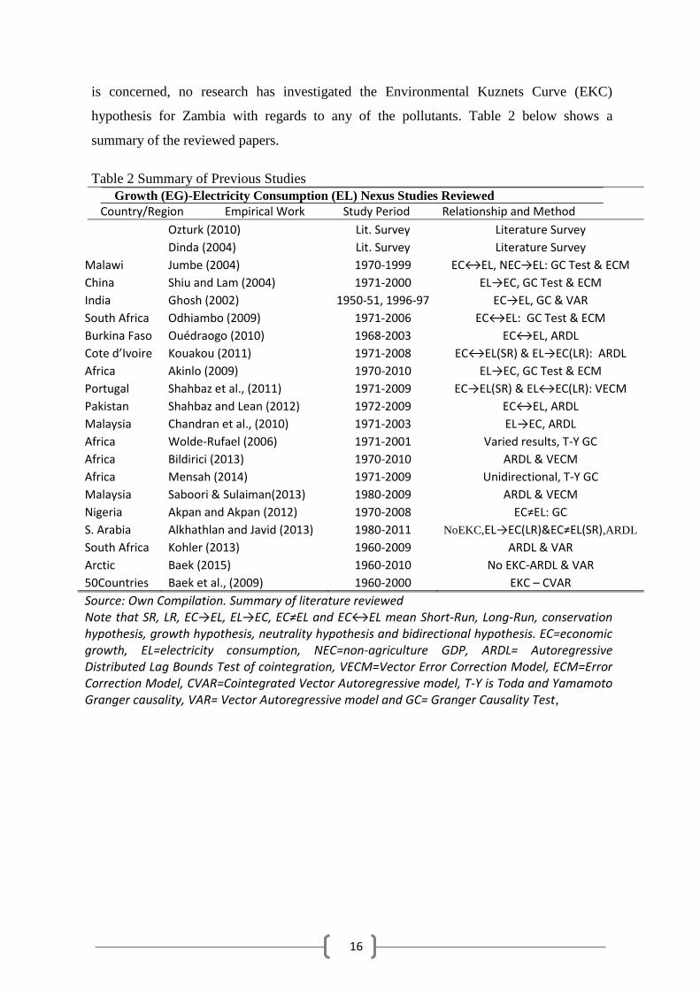
hypothesis for Zambia with regards to any of the pollutants. Table 2 below shows a
summary of the reviewed papers.
Table 2 Summary of Previous Studies
Growth (EG)-Electricity Consumption (EL) Nexus Studies Reviewed
Country/Region Empirical Work Study Period Relationship and Method
Ozturk (2010) Lit. Survey Literature Survey
Dinda (2004) Lit. Survey Literature Survey
Malawi Jumbe (2004) 1970-1999 EC↔EL, NEC→EL: GC Test & ECM
China Shiu and Lam (2004) 1971-2000 EL→EC, GC Test & ECM
India Ghosh (2002) 1950-51, 1996-97 EC→EL, GC & VAR
South Africa Odhiambo (2009) 1971-2006 EC↔EL: GC Test & ECM
Burkina Faso Ouédraogo (2010) 1968-2003 EC↔EL, ARDL
Cote d’Ivoire Kouakou (2011) 1971-2008 EC↔EL(SR) & EL→EC(LR): ARDL
Africa Akinlo (2009) 1970-2010 EL→EC, GC Test & ECM
Portugal Shahbaz et al., (2011) 1971-2009 EC→EL(SR) & EL↔EC(LR): VECM
Pakistan Shahbaz and Lean (2012) 1972-2009 EC↔EL, ARDL
Malaysia Chandran et al., (2010) 1971-2003 EL→EC, ARDL
Africa Wolde-Rufael (2006) 1971-2001 Varied results, T-Y GC
Africa Bildirici (2013) 1970-2010 ARDL & VECM
Africa Mensah (2014) 1971-2009 Unidirectional, T-Y GC
Malaysia Saboori & Sulaiman(2013) 1980-2009 ARDL & VECM
Nigeria Akpan and Akpan (2012) 1970-2008 EC≠EL: GC
S. Arabia Alkhathlan and Javid (2013) 1980-2011 NoEKC,EL→EC(LR)&EC≠EL(SR),ARDL
South Africa Kohler (2013) 1960-2009 ARDL & VAR
Arctic Baek (2015) 1960-2010 No EKC-ARDL & VAR
50Countries Baek et al., (2009) 1960-2000 EKC – CVAR
Source: Own Compilation. Summary of literature reviewed Note that SR, LR, EC→EL, EL→EC, EC≠EL and EC↔EL mean Short-Run, Long-Run, conservation hypothesis, growth hypothesis, neutrality hypothesis and bidirectional hypothesis. EC=economic growth, EL=electricity consumption, NEC=non-agriculture GDP, ARDL= Autoregressive Distributed Lag Bounds Test of cointegration, VECM=Vector Error Correction Model, ECM=Error Correction Model, CVAR=Cointegrated Vector Autoregressive model, T-Y is Toda and Yamamoto Granger causality, VAR= Vector Autoregressive model and GC= Granger Causality Test,
17
3.0 Methodology
In this section, the paper presents brief theoretical underpinnings for the study of pollution,
income and electricity consumption in the context of trade. The econometric strategy that is
applied in this research is then explained in the following subsection. Thus, the section
starts with a theory based on the Green Solow model and static general equilibrium model.
Later a discussion of the econometric estimation procedure that is applied in the study is
provided. The estimation approach is to check for the time-series properties of the data to
determine the appropriate time series model to use for the analysis, followed by
cointegration analysis to determine if the variables in the model do have a long-run
relationship. This second step is conditional on the outcome of the first and if the series are
not stationary, then the second step become important to avoid estimating and reporting
spurious regression. The next step in the econometric strategy is to determine the
appropriate model given the outcome in step (1) and (2). If the variables are found to be
non-stationary but cointegrated, the OLS estimated in such instances are consistent
estimators, but if some of the variables are potentially endogenous, the OLS estimator will
suffer from endogenous bias and also prone to first order serial correlation issues.
Therefore, in this step, Dynamic Ordinary Least Square (DOLS) is the choice of the
estimator for the long-run analysis since it has the good properties of the OLS and also
correct for some of the bad properties as alluded above. In the final step, a causality
analysis is undertaken along short-run analysis, which a Vector Error Correction Model
(VECM) is the choice of model for this due to the efficiency argument when variables are
cointegrated.
3.1 Theoretical Underpinnings
The theoretical models adopted in this paper are based on Brock and Taylor (2010),
Johansson and Kriström (2007) and Stefanski (2013). These are the Solow growth model
and the simple static general equilibrium model.
In the Solow growth model, the supply of goods and services is based on a constant returns
to scale production function while the demand side is based on the equality of savings and
investments (Mankiw, 2009). Thus, on the supply side of the Solow growth model, an
economy combines factors of production such as capital (𝐾𝑡), labour (𝐿𝑡) and technology
(𝐴𝑡) to produce an output which translates into the income of the economy (Romer, 1996).
And on the demand side, the income from production is either consumed or invested and
18
over time capital stock is key to determining the economy’s output (Mankiw, 2009).
Therefore, as capital accumulates in the economy over time, the economy begins to
approach a steady state via the balanced growth path.
Nonetheless, the Solow growth model has been extended to an augmented Green Solow
growth model where exogenous technological progress in both abatement and goods
production tends to lead to continued growth with rising environmental quality (Brock and
Taylor, 2010). This extension is the one that explains the existence of the environmental
Kuznets curve hypothesis. Therefore, along a growth path with capital accumulation,
environmental quality tends to rise eventually.
The Green Solow growth model is based on a number of assumptions which play key roles.
The Green Solow growth model assumes fixed savings, depreciation and abatement
intensity, all of which are determined exogenously (Brock and Taylor, 2010; Mankiw,
2009; Stefanski, 2013). Additionally, labour (𝐿𝑡), labour productivity(𝜏𝑡), depreciation and
exogenous technological progress in abatement are also assumed to grow at constant rates
of n, g, 𝛿 and 𝑔𝐴 respectively (Stefanski, 2013). As stated, the output is assumed to be
produced by the utilisation of capital, labour and technology inherent in the production
function, i.e., 𝐹(𝐾𝑡, 𝜏𝑡𝐿𝑡) where 𝜏𝑡 is labour productivity. It is further assumed that the
economy can allocate a fixed fraction of output (𝜗) for abatement where the fraction falls in
the interval 0 < 𝜗 < 1 (Brock and Taylor, 2010).
With the above underlying assumptions, pollution of Ω𝑡 units at a point in time is assumed
to be the by-product of the production process and this assumption is the main departure
from the traditional Solow growth model (Stefanski, 2013). Therefore, the Ω𝑡 units of
pollution are the amount emitted without abatement, and 𝑎(𝜗)Ω𝑡 are the amount emitted
with abatements in place. Moreover, the abatement function, 𝑎(𝜗), is assumed to satisfy a
positive diminishing marginal impact on pollution by concavity, i.e., 𝑎(0) = 1, 𝑎′(𝜗) < 0
and 𝑎′′(𝜗) > 0 (Brock and Taylor, 2010). Combining the assumptions on abatement and
pollution then produces the following model;
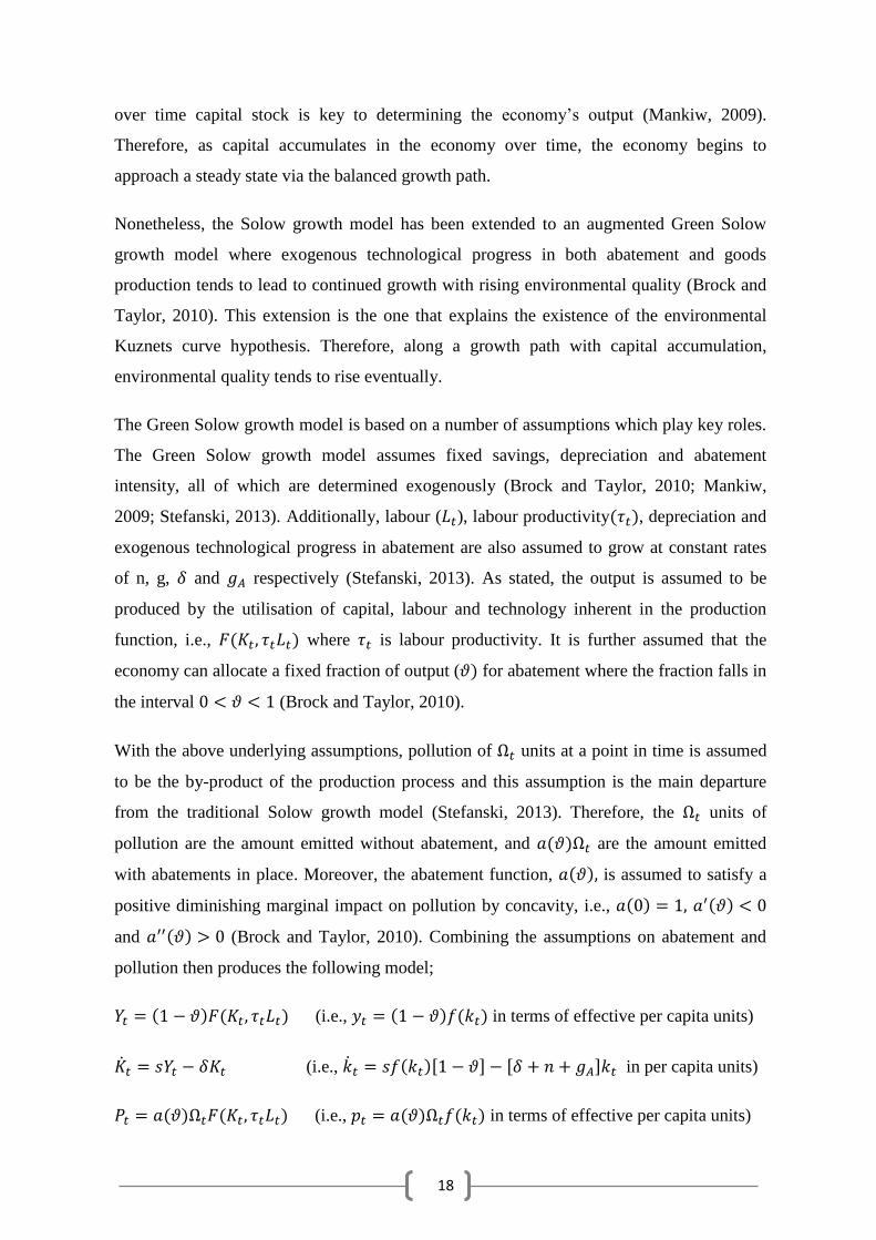
𝑌𝑡 = (1 − 𝜗)𝐹(𝐾𝑡, 𝜏𝑡𝐿𝑡) (i.e., 𝑦𝑡 = (1 − 𝜗)𝑓(𝑘𝑡) in terms of effective per capita units)
�̇�𝑡 = 𝑠𝑌𝑡 − 𝛿𝐾𝑡 (i.e., �̇�𝑡 = 𝑠𝑓(𝑘𝑡)[1 − 𝜗] − [𝛿 + 𝑛 + 𝑔𝐴]𝑘𝑡 in per capita units)
𝑃𝑡 = 𝑎(𝜗)Ω𝑡𝐹(𝐾𝑡, 𝜏𝑡𝐿𝑡) (i.e., 𝑝𝑡 = 𝑎(𝜗)Ω𝑡𝑓(𝑘𝑡) in terms of effective per capita units)
19
�̇�𝑡 = 𝑛𝐿𝑡, 𝜏�̇� = 𝑔𝜏𝑡 and Ω̇𝑡 = −𝑔𝐴Ω𝑡
Where the dot above the variable represents the partial difference with respect to time. The
first line (i.e., 𝑌𝑡) depicts the output available for investment and consumption with the
consideration of the abatement assumptions. The second line (i.e., �̇�𝑡) shows that capital
accumulates based on the difference between savings and depreciation, and the third line
(i.e., 𝑃𝑡) shows that pollution is a function of output and abatement.
The dynamics of the environmental Kuznets curve are driven by capital accumulation in the
Green Solow growth model (Stefanski, 2013). As stated earlier, when the economy grows
capital accumulation tends to approach the steady state level. Thus, as the economy
approaches the balanced growth path the aggregate output, consumption and capital all
grow at 𝑔 + 𝑛 (i.e., where 𝑔 is growth in augmented labour technology and 𝑛 is the growth
of labour). On the other hand, the respective effective per capita counterpart terms grow at
𝑔𝑦 = 𝑔𝑐 = 𝑔𝑘 = 𝑔 > 0. The growth rate of aggregate pollution (i.e., 𝑔𝑝) can thus be
inferred from the fact that capital accumulation approaches the constant 𝑘∗ at the steady
state (Brock and Taylor, 2010). This growth of aggregate pollution is growth in aggregate
capital (or output or consumption) less growth in abatement technology along the balanced
growth path exemplified as;
𝑔𝑝 = 𝑔 + 𝑛 − 𝑔𝐴𝑇
Where 𝑔𝐴𝑇 is growth in abatement technology. Therefore, 𝑔 + 𝑛 and 𝑔𝐴𝑇 are scale effect
of growth on emissions and the technique effect respectively (Brock and Taylor, 2010).
International trade, on the other hand, can influence factor productivity and lead to
technological change via the conventional production function 𝐹(𝐾𝑡, 𝜏𝑡𝐿𝑡). This implies
that foreign trade influences income through technological progress in both factor
productivity and the production technology but may also influence pollution through the
progress of the existing abatement technology. The increased income motivates for more
energy use due to relatively higher disposable income which results in the acquisition of
more electricity dependent gadgets. Also, every production process requires energy services
and therefore energy is an important input requirement in production. This, among other
things, implies greater economic activity is likely to result in more use of energy.
20
The shape of the environmental Kuznets curve (EKC) is dependent on the diminishing
marginal returns and technological progress. The fact that capital accumulation only affects
economic growth rate implies that the accumulation of capital impacts on growth less at the
steady state than when capital is accumulating. Therefore, countries off the balanced growth
path grow faster than those on the balanced growth path (Brock and Taylor, 2010). The
environmental Kuznets curve (EKC) hypothesises an inverted U-shaped relationship
between pollution and income in which environmental degradation tends to; become worse
as a nation grows out of poverty; stabilises at some middle income and then gradually
reduces after some threshold (Kohler, 2013).
However, a policy conclusion is that there is no presumption that the environmental
Kuznets curve has an inverted U-shape, and no country should wait as they try to grow out
of the environmental problems (Johansson and Kriström, 2007). Therefore, no country
should wait for environmental problems to ease out when they can alternatively institute
policies that would work towards reducing environmental damage. The EKC hypothesis
grew out of the debate opposing the long-standing view that economic activity inevitably
hurts the environment (Perman and Perman, 2011). Therefore, capital accumulation and the
growth path of an economy motivate the existence of the Environmental Kuznets Curve
(EKC) hypothesis.
Furthermore, the environmental Kuznets curve can also be explained using the interaction
of the producer and consumer theories. Thus, given the production function, a simple
general equilibrium model can be obtained by considering the representative consumer’s
utility function. Johansson and Kriström (2007) provide a simple static general equilibrium
model with exogenous technological progress using a utility function for a representative
consumer and a concave production function. According to Johansson and Kriström (2007),
the utility function of the representative consumer can include two arguments, consumption
(c) and pollution (p) such as,
𝑈(𝑐, 𝑝) (1)
Where it is assumed that 𝜕𝑈
𝜕𝑐= 𝑈𝑐 > 0 and
𝜕𝑈
𝜕𝑝= 𝑈𝑝 < 0 and further assumed that
𝜕2𝑈
𝜕𝑐2=
𝑈𝑐𝑐 < 0 and 𝑑2𝑈
𝑑𝑝2= 𝑈𝑝𝑝 > 0. Abstracting from capital, and labour in the concave
production function and focusing on technology (A) and pollution (p) (i.e., c=f(p,A), it is
21
possible to construct society’s maximisation problem. Thus, the maximisation problem
becomes
Maximise: 𝑈(𝑐, 𝑝) Subject to: 𝑐 = 𝑓(𝑝, 𝐴)
which can be solved using the Lagrange method as;
𝐿 = 𝑈(𝑐, 𝑝) + 𝜆(𝑐 − 𝑓(𝑝, 𝐴) with first order conditions (FOC) yielding;
𝜕𝐿
𝜕𝑐= 𝑈𝑐 + 𝜆 = 0,
𝜕𝐿
𝜕𝑝= 𝑈𝑝 − 𝜆𝑓𝑝(𝑝, 𝐴) = 0 and
𝜕𝐿
𝜕𝑐= 𝑐 − 𝑓(𝑝, 𝐴) = 0 (2)
where the first order conditions yield;
FOC:−𝑈𝑝
𝑈𝑐= 𝑓𝑝 (3)
The first order condition (3) gives the marginal willingness to pay (MWTP) to reduce
pollution for each given technology which is equal to the marginal product lost when
reducing pollution. Consequently, the point at which the marginal willingness to pay for
reduced pollution is equal to the lost marginal product represents some of the points on the
environmental Kuznets curve. The environmental Kuznets curve can be viewed as a form of
an equilibrium relationship arising from the combination of technology and preferences
(Johansson and Kriström, 2007).
The idea behind this process is that production process of a ‘good’ is usually associated
with the production of a ‘bad’ as a by-product and the evolution of technological progress
over time enables more production at each level of emissions (Ankarhem, 2005). This
technological progress over time inevitably creates the counteractions of the substitution
and income effects. Therefore, the environmental Kuznets curve hypothesis is captured by
the marginal rate of substitution between consumption and pollution, and the hypothesis
can be explained in terms of substitution and income effects (Johansson and Kriström,
2007). Thus, the expansion path of the interaction of producer and consumer theory (i.e.,
with the individual points represented by −𝑈𝑝
𝑈𝑐= 𝑓𝑝) is shown in the graph as the curve A-
B, which, traces out the inverted U-shaped curve as shown in Figure 3.
22
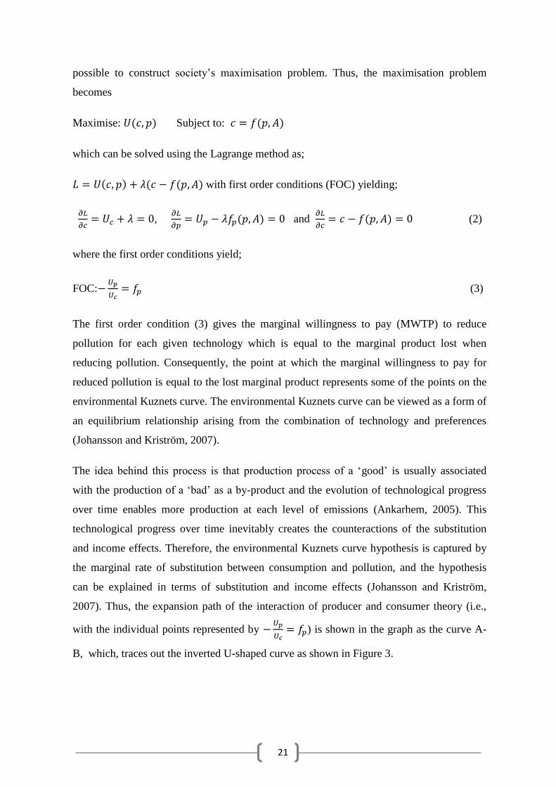
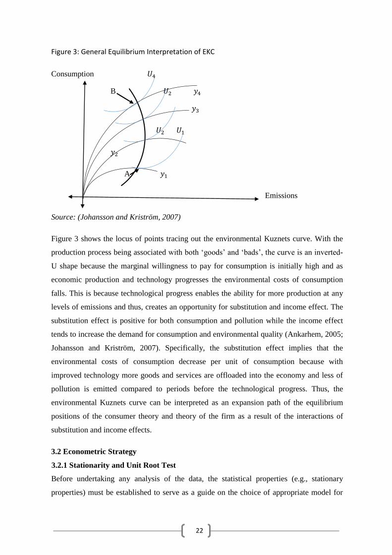
Figure 3: General Equilibrium Interpretation of EKC
Consumption 𝑈4
B 𝑈2 𝑦4
𝑦3
𝑈2 𝑈1
𝑦2
A 𝑦1
Emissions
Source: (Johansson and Kriström, 2007)
Figure 3 shows the locus of points tracing out the environmental Kuznets curve. With the
production process being associated with both ‘goods’ and ‘bads’, the curve is an inverted-
U shape because the marginal willingness to pay for consumption is initially high and as
economic production and technology progresses the environmental costs of consumption
falls. This is because technological progress enables the ability for more production at any
levels of emissions and thus, creates an opportunity for substitution and income effect. The
substitution effect is positive for both consumption and pollution while the income effect
tends to increase the demand for consumption and environmental quality (Ankarhem, 2005;
Johansson and Kriström, 2007). Specifically, the substitution effect implies that the
environmental costs of consumption decrease per unit of consumption because with
improved technology more goods and services are offloaded into the economy and less of
pollution is emitted compared to periods before the technological progress. Thus, the
environmental Kuznets curve can be interpreted as an expansion path of the equilibrium
positions of the consumer theory and theory of the firm as a result of the interactions of
substitution and income effects.
3.2 Econometric Strategy
3.2.1 Stationarity and Unit Root Test
Before undertaking any analysis of the data, the statistical properties (e.g., stationary
properties) must be established to serve as a guide on the choice of appropriate model for
23
the analysis. The paper employs two unit root tests, the Augmented Dickey-Fuller (ADF)
test, and the Phillips-Perron (PP) test to establish the stationary properties of the variables.
According to Gujarati and Porter (2009) the Augmented Dickey-Fuller test consists of
estimating the regression such as;
Δ𝑦𝑡 = 𝛽1 + 𝛽2𝑡 + 𝛿𝑦𝑡−1 + ∑ 𝛼𝑖𝑚𝑖=1 ∆𝑦𝑡−1 + 휀𝑡 (4)
The null hypothesis is that there is no stationarity (i.e., 𝛿 = 0) in the variables while the
alternative is that there is stationarity (i.e., 𝛿 < 0). However, the Augmented Dickey-Fuller
(ADF) test is mostly considered a non-robust test for unit root (Ouédraogo, 2010). So, to be
sure an additional test for the unit root, the Phillips-Perron (PP) test, is undertaken. The
Phillips-Perron test is a non-parametric statistical method that takes care of serial
correlation without using the lagged differences of the dependent variable (Gujarati and
Porter, 2009). Therefore, the Phillips-Perron test is considered an alternative as it allows for
milder assumptions on the distribution of errors and presents an opportunity to control for
higher order serial correlation in the time series variables and is robust against
heteroscedasticity (Kouakou, 2011). Therefore, the Augmented Dickey-Fuller test and the
Phillips-Perron test are used in this study to check for stationarity.
3.2.2 Cointegration Tests
Theoretical developments have raised the possibility that two or more integrated,
nonstationary time series might be cointegrated so that some linear combination of these
series could be stationary even though each independent series is not (Engle and Granger,
1987). Given that the Environmental Kuznets Curve (EKC) hypothesis and the trade-
income-emission phenomena are both long-run concepts, it is important to test for
cointegration if these variables are nonstationary to avoid reporting spurious long-run
relationships. The cointegration approach is desirable to getting a clear picture of the long-
run relationship between the variables of interest for nonstationary variables (Baek, 2015;
Baek et al., 2009). Cointegration analysis thus, allows us to check for long-run relationships
among the variables. Lütkepohl, (2005) and Lütkepohl et al. (2001) point out that
cointegration is checked by undertaking two kinds of Likelihood Ratio tests, the Trace test
and the Maximum Eigenvalue tests of the form;
24
𝜆𝑡𝑟𝑎𝑐𝑒(𝑟) = −𝑇∑ log(1 − 𝜆𝑗)𝑛𝑗=𝑟+1 and 𝜆𝑚𝑎𝑥(𝑟) = −𝑇log(1 − 𝜆𝑟+1) respectively4.
In this vein, the associated hypotheses for the Trace statistic and the Maximum Eigenvalue
test are respectively given by;
Trace: 𝐻𝑜(𝑟): 𝑟𝑘(Π) = 𝑟 𝑉𝑠. 𝐻1(𝑟): 𝑟𝑘(Π) > 𝑟
Max. Eigenvalue: 𝐻𝑜(𝑟): 𝑟𝑘(Π) = 𝑟 𝑉𝑠. 𝐻1(𝑟 + 1): 𝑟𝑘(Π) = 𝑟 + 1.
Therefore, long-run relationships are determined by the two tests of the respectively
associated hypotheses. The null hypothesis can be interpreted as no cointegration (i.e., no
long-run relation) while the alternative as having at least one cointegrating equation(i.e.,
long-run relationship).
3.2.3 Long-Run Model
The long-run model in this study is a logarithmic, quadratic function (i.e., for carbon
emission) as shown below. The three logarithmic, quadratic functions respectively make
use of different versions of electricity consumption, i.e., total electricity consumption (lnet),
industrial electricity consumption (lnem) and residential and agricultural electricity
consumption (lner). This means that besides the model that makes use of total electricity,
the long-run model also considers disaggregated sector-level of electricity use (industrial
and combined residential and agricultural electricity use). As alluded to in the introduction,
most studies about energy consumption, income, and carbon dioxide (CO2) emissions
suffer the problem of aggregation bias (Baek, 2015). That is most studies apply energy
consumption in its totality as opposed to energy consumption by sectors. Therefore, having
an analysis for both the aggregated (i.e., total) and disaggregated (i.e., in sectors) electricity
consumption (i.e., in sectors) enables the study to counter this perceived weakness.
The three models are shown below;
lnc𝑡 = 𝛽0 + 𝛽1lny𝑡 + 𝛽2(lny𝑡)2 + 𝛽3lnet𝑡 + 𝛽4lnf𝑡 + 휀𝑡;
lnc𝑡 = 𝛽0 + 𝛽1lny𝑡 + 𝛽2(lny𝑡)2 + 𝛽3lnem𝑡 + 𝛽4lnf𝑡 + 휀𝑡;
4 where 𝜆1 ≥ ⋯ ≥ 𝜆𝑛 are ordered generalised eigenvalues found by solving the det(𝜆𝑆11 −
𝑆10𝑆00−1𝑆01) in which 𝑆𝑖𝑗 = 𝑇
−1∑ 𝑅0𝑡𝑅1𝑡𝑇𝑡=1 and 𝑅0𝑡, 𝑅0𝑡 are residual from the regressions of Δ𝑦𝑡
and 𝑦𝑡−1.
25
lnc𝑡 = 𝛽0 + 𝛽1lny𝑡 + 𝛽2(lny𝑡)2 + 𝛽3lner𝑡 + 𝛽4lnf𝑡 + 휀𝑡;
where lnyt, lnet, lnct, lnft (lny𝑡)2 and 휀𝑡 represent the natural logs of real gross domestic
product(GDP), electricity consumption (i.e., total, industrial and Residential & agricultural
being lnet𝑡, lnem𝑡 and lner𝑡 respectively ) carbon emissions, foreign trade, square of
income (i.e., GDP) and the error term respectively. Additionally, 𝛽1, 𝛽2, 𝛽3 and 𝛽4 are the
coefficients of income, income squared, electricity use and foreign trade, respectively. For
the environmental Kuznets curve (EKC) hypothesis, there are several possible expected
results that can be obtained from the estimations of the above models (Dinda, 2004). Below
are some of the expected relationships
(i) 𝛽1 = 𝛽2 = 𝛽3 = 𝛽4 = 0; This result is synonymous to a neutrality hypothesis as it
implies that there is no relationship between carbon emissions and; income, income
squared, electricity consumptions and foreign trade. This null hypothesis signifies
that there is no environmental Kuznets curve hypothesis present in the data.
Therefore, failure to reject this hypothesis would mean the absence of the
environmental Kuznets curve hypothesis and a rejection would be a signal of either
inverted U-shaped curve (i.e., EKC) or the U-shaped curve.
(ii) 𝛽1 > 0, 𝛽2 = 𝛽3 = 𝛽4 = 0; This is a monotonic increasing relationship between
carbon emissions and income. This implies higher incomes lead to higher carbon
emissions. In terms of EKC, the null hypothesis is that there is no environmental
kuznetc curve hypothesis present but rather a positive linear relationship.
(iii) 𝛽1 > 0, 𝛽2 < 0, 𝛽3 = 𝛽4 = 0; This is the case of the inverted U-shaped curve
relationship between the carbon emissions and income. Therefore, this is the case
of the environmental Kuznets curve (EKC) hypothesis. Thus, the null hypothesis is
that there is the presence of environmental Kuznets curve hypothesis and, rejection
of this null hypothesis would mean that the environmental Kuznets curve
phenomena are absent.
(iv) 𝛽1 < 0, 𝛽2 > 0, 𝛽3 = 𝛽4 = 0; This is the opposite of the environmental Kuznets
curve (EKC) hypothesis where the relationship between carbon emissions and
income is U-shaped. Therefore, the null hypothesis is that there is the presence of a
U-shaped curve as opposed to an inverted U-shaped curve. This means that the null
hypothesis is that environmental Kuznets curve hypothesis is absent. Thus, failure
26
to reject this null hypothesis would mean that there is no presence of the
environmental Kuznets curve hypothesis.
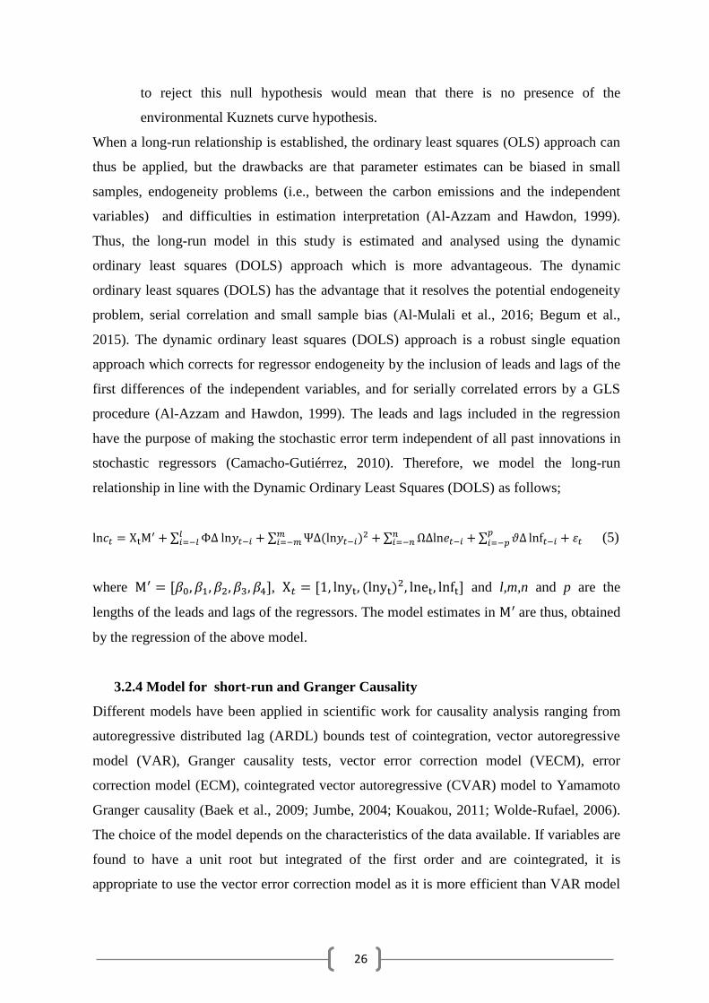
When a long-run relationship is established, the ordinary least squares (OLS) approach can
thus be applied, but the drawbacks are that parameter estimates can be biased in small
samples, endogeneity problems (i.e., between the carbon emissions and the independent
variables) and difficulties in estimation interpretation (Al-Azzam and Hawdon, 1999).
Thus, the long-run model in this study is estimated and analysed using the dynamic
ordinary least squares (DOLS) approach which is more advantageous. The dynamic
ordinary least squares (DOLS) has the advantage that it resolves the potential endogeneity
problem, serial correlation and small sample bias (Al-Mulali et al., 2016; Begum et al.,
2015). The dynamic ordinary least squares (DOLS) approach is a robust single equation
approach which corrects for regressor endogeneity by the inclusion of leads and lags of the
first differences of the independent variables, and for serially correlated errors by a GLS
procedure (Al-Azzam and Hawdon, 1999). The leads and lags included in the regression
have the purpose of making the stochastic error term independent of all past innovations in
stochastic regressors (Camacho-Gutiérrez, 2010). Therefore, we model the long-run
relationship in line with the Dynamic Ordinary Least Squares (DOLS) as follows;
ln𝑐𝑡 = XtM′ + ∑ ΦΔ ln𝑦𝑡−𝑖 + ∑ ΨΔ(ln𝑦𝑡−𝑖)
2𝑚𝑖=−𝑚 +∑ ΩΔln𝑒𝑡−𝑖
𝑛𝑖=−𝑛 +∑ 𝜗Δ
𝑝𝑖=−𝑝 lnf𝑡−𝑖 + 휀𝑡
𝑙𝑖=−𝑙 (5)
where M′ = [𝛽0, 𝛽1, 𝛽2, 𝛽3, 𝛽4], X𝑡 = [1, lnyt, (lnyt)2, lnet, lnft] and l,m,n and p are the
lengths of the leads and lags of the regressors. The model estimates in M′ are thus, obtained
by the regression of the above model.
3.2.4 Model for short-run and Granger Causality
Different models have been applied in scientific work for causality analysis ranging from
autoregressive distributed lag (ARDL) bounds test of cointegration, vector autoregressive
model (VAR), Granger causality tests, vector error correction model (VECM), error
correction model (ECM), cointegrated vector autoregressive (CVAR) model to Yamamoto
Granger causality (Baek et al., 2009; Jumbe, 2004; Kouakou, 2011; Wolde-Rufael, 2006).
The choice of the model depends on the characteristics of the data available. If variables are
found to have a unit root but integrated of the first order and are cointegrated, it is
appropriate to use the vector error correction model as it is more efficient than VAR model
27
in such cases. However, the difficulties of using vector autoregressive models when
variables have a unit root and yet are integrated of the first order (i.e., I(1) ) are spelt out in
(Granger and Newbold, 1974).
Most studies on the causal relationship between electricity consumption and economic
growth employ the Granger causality and error correction model (ECM) in their
investigation (Ghosh, 2002), Shiu and Lam (2004), Kouakou (2011)). This paper applies a
similar approach, though by using the vector error correction model. In error correction
models, changes in variables depend on deviations from some equilibrium relation
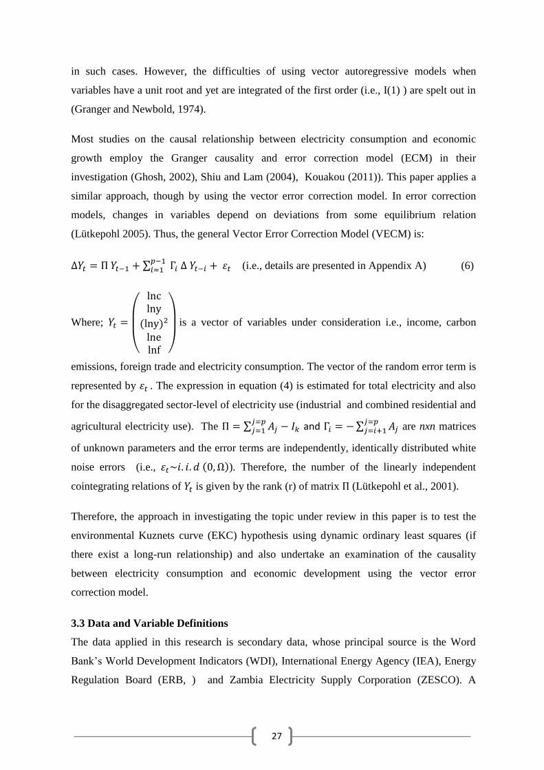
(Lütkepohl 2005). Thus, the general Vector Error Correction Model (VECM) is:
∆𝑌𝑡 = Π 𝑌𝑡−1 + ∑ Γ𝑖 Δ 𝑌𝑡−𝑖𝑝−1𝑖=1 + 휀𝑡 (i.e., details are presented in Appendix A) (6)
Where; 𝑌𝑡 =
(
lnclny
(lny)2
lnelnf )
is a vector of variables under consideration i.e., income, carbon
emissions, foreign trade and electricity consumption. The vector of the random error term is
represented by 휀𝑡 . The expression in equation (4) is estimated for total electricity and also
for the disaggregated sector-level of electricity use (industrial and combined residential and
agricultural electricity use). The Π = ∑ 𝐴𝑗 − 𝐼𝑘𝑗=𝑝𝑗=1 and Γ𝑖 = −∑ 𝐴𝑗
𝑗=𝑝𝑗=𝑖+1 are nxn matrices
of unknown parameters and the error terms are independently, identically distributed white
noise errors (i.e., 휀𝑡~𝑖. 𝑖. 𝑑 (0, Ω)). Therefore, the number of the linearly independent
cointegrating relations of 𝑌𝑡 is given by the rank (r) of matrix Π (Lütkepohl et al., 2001).
Therefore, the approach in investigating the topic under review in this paper is to test the
environmental Kuznets curve (EKC) hypothesis using dynamic ordinary least squares (if
there exist a long-run relationship) and also undertake an examination of the causality
between electricity consumption and economic development using the vector error
correction model.
3.3 Data and Variable Definitions
The data applied in this research is secondary data, whose principal source is the Word
Bank’s World Development Indicators (WDI), International Energy Agency (IEA), Energy
Regulation Board (ERB, ) and Zambia Electricity Supply Corporation (ZESCO). A
28
summary of the raw data that was used for this research is provided in Appendix C. The
empirical study uses a forty-year time series data for the period between 1971-2010 for
electricity consumption, trade, carbon emissions and real gross domestic product.
The electricity consumption is divided into total electricity consumption (et), industrial
electricity consumption (em), and residential and agriculture electricity consumption (er).
Residential and agricultural electricity consumptions were added together because it is
believed that most residential households are engaged in agriculture. This close association
makes the distinction between the two forms of electricity consumption very difficult,
therefore, justifying the combination of agriculture consumption and residential
consumption into one.
Industrial electricity consumption is defined as being composed of electricity consumption
from mining and quarry, the transportation, services (i.e., private and public sectors) and all
other industrial sectors. While the residential and agriculture electricity consumption is self-
explanatory as it comprises the consumption related to residential and agricultural
electricity use. The total electricity consumption comprises the total of all electricity use in
the economy of Zambia. Since convention in most applied work is to use the electricity
consumption in terms of kilowatt-hour that is followed in this research as well (Akinlo,
2009; Jumbe, 2004; Shahbaz et al., 2011; Shahbaz and Lean, 2012; Wolde-Rufael, 2006).
Thus, raw electricity consumption data was initially measured in terajoules from
International Energy Administration (IEA), Energy Regulation Board (ERB) and Zambia
Electricity Supply Corporation (ZESCO). All the values were transformed by multiplying
them by 277777.8 to obtain kilowatt-hour (kWh) figures.
On the other hand, foreign trade, carbon emissions and gross domestic product were
obtained from the world development indicators (WDI). For a proxy of trade openness, the
paper makes use of foreign trade in the form of exports plus imports while for pollution,
carbon emissions in metric tonnes are used. According to the World Bank’s world
development indicators, carbon emissions are defined as those due to the burning of fossil
fuels and the manufacture of cement (World Bank, n.d.). Additionally, the real gross
domestic product has been defined as the sum of the gross value added by all resident
producers in the economy plus any product taxes less any subsidies, i.e., in the local
currency Zambian Kwacha (World Bank, n.d.).
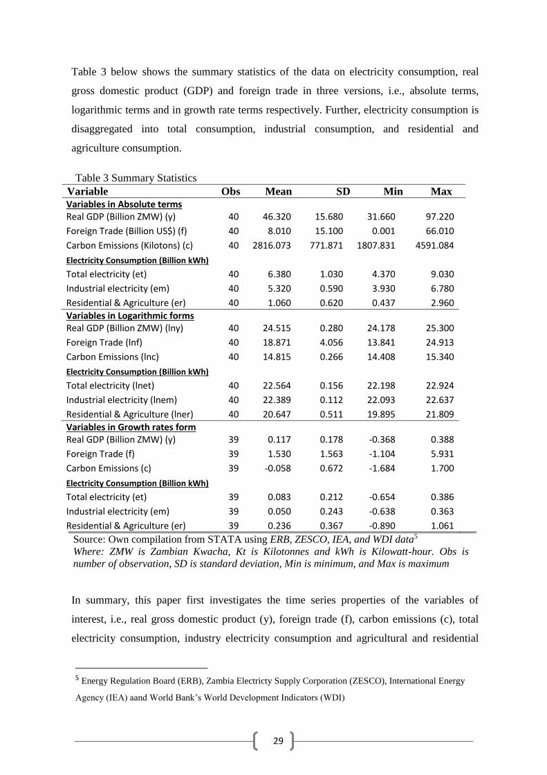
29
Table 3 below shows the summary statistics of the data on electricity consumption, real
gross domestic product (GDP) and foreign trade in three versions, i.e., absolute terms,
logarithmic terms and in growth rate terms respectively. Further, electricity consumption is
disaggregated into total consumption, industrial consumption, and residential and
agriculture consumption.
Table 3 Summary Statistics
Variable Obs Mean SD Min Max
Variables in Absolute terms Real GDP (Billion ZMW) (y) 40 46.320 15.680 31.660 97.220
Foreign Trade (Billion US$) (f) 40 8.010 15.100 0.001 66.010
Carbon Emissions (Kilotons) (c) 40 2816.073 771.871 1807.831 4591.084
Electricity Consumption (Billion kWh) Total electricity (et) 40 6.380 1.030 4.370 9.030
Industrial electricity (em) 40 5.320 0.590 3.930 6.780
Residential & Agriculture (er) 40 1.060 0.620 0.437 2.960
Variables in Logarithmic forms Real GDP (Billion ZMW) (lny) 40 24.515 0.280 24.178 25.300
Foreign Trade (lnf) 40 18.871 4.056 13.841 24.913
Carbon Emissions (lnc) 40 14.815 0.266 14.408 15.340
Electricity Consumption (Billion kWh) Total electricity (lnet) 40 22.564 0.156 22.198 22.924
Industrial electricity (lnem) 40 22.389 0.112 22.093 22.637
Residential & Agriculture (lner) 40 20.647 0.511 19.895 21.809
Variables in Growth rates form Real GDP (Billion ZMW) (y) 39 0.117 0.178 -0.368 0.388
Foreign Trade (f) 39 1.530 1.563 -1.104 5.931
Carbon Emissions (c) 39 -0.058 0.672 -1.684 1.700
Electricity Consumption (Billion kWh) Total electricity (et) 39 0.083 0.212 -0.654 0.386
Industrial electricity (em) 39 0.050 0.243 -0.638 0.363
Residential & Agriculture (er) 39 0.236 0.367 -0.890 1.061
Source: Own compilation from STATA using ERB, ZESCO, IEA, and WDI data5
Where: ZMW is Zambian Kwacha, Kt is Kilotonnes and kWh is Kilowatt-hour. Obs is
number of observation, SD is standard deviation, Min is minimum, and Max is maximum
In summary, this paper first investigates the time series properties of the variables of
interest, i.e., real gross domestic product (y), foreign trade (f), carbon emissions (c), total
electricity consumption, industry electricity consumption and agricultural and residential
5 Energy Regulation Board (ERB), Zambia Electricty Supply Corporation (ZESCO), International Energy
Agency (IEA) aand World Bank’s World Development Indicators (WDI)
30
electricity consumption. Consequently, the unit root tests for all the variables are done, and
the appropriate order of integration is determined. The appropriate lag orders are then
determined for the respective models under investigation. If the variables reveal
nonstationary properties, a cointegration test is performed to establish whether a long-run
relationship between the variables in the model exists.
The vector error correction model presented in equation (6) is used for the Granger
causality test. The causality relationship in the equation can be inferred to be either of forms
of the discussed outcomes of growth, conservation, neutrality, and bidirectional hypotheses.
Since the vector error correction model (VECM) only gives an estimation of coefficients
and the long-run relationship, the direction of causality is deduced from the Granger
causality test. If the time series under review are not found to be cointegrated the causality
is performed as a vector autoregressive (VAR) in first difference form, otherwise the
causality is conducted with the inclusion of the error correction term (Chandran et al., 2010;
Kouakou, 2011; Saboori and Sulaiman, 2013; Shahbaz et al., 2011; Shahbaz and Lean,
2012). The causality test is conducted for the three models, consisting of total and two
different sectors of electricity consumption.
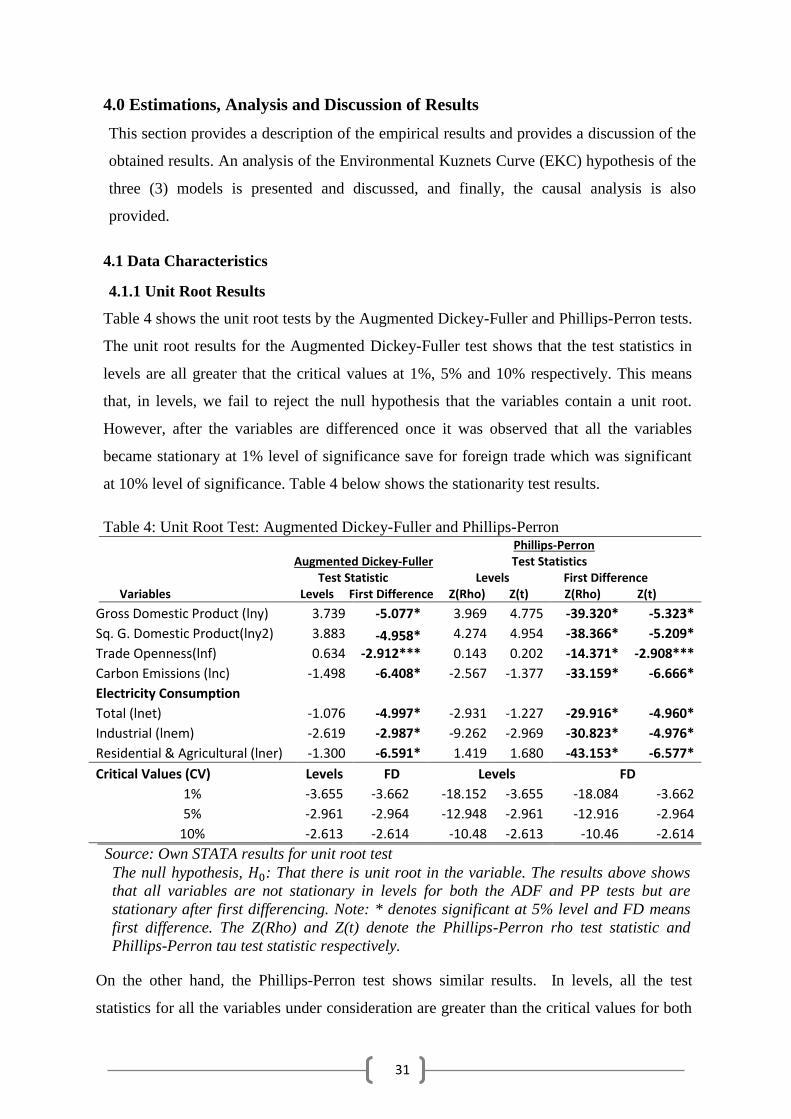
31
4.0 Estimations, Analysis and Discussion of Results
This section provides a description of the empirical results and provides a discussion of the
obtained results. An analysis of the Environmental Kuznets Curve (EKC) hypothesis of the
three (3) models is presented and discussed, and finally, the causal analysis is also
provided.
4.1 Data Characteristics
4.1.1 Unit Root Results
Table 4 shows the unit root tests by the Augmented Dickey-Fuller and Phillips-Perron tests.
The unit root results for the Augmented Dickey-Fuller test shows that the test statistics in
levels are all greater that the critical values at 1%, 5% and 10% respectively. This means
that, in levels, we fail to reject the null hypothesis that the variables contain a unit root.
However, after the variables are differenced once it was observed that all the variables
became stationary at 1% level of significance save for foreign trade which was significant
at 10% level of significance. Table 4 below shows the stationarity test results.
Table 4: Unit Root Test: Augmented Dickey-Fuller and Phillips-Perron Phillips-Perron Augmented Dickey-Fuller Test Statistics Test Statistic Levels First Difference Variables Levels First Difference Z(Rho) Z(t) Z(Rho) Z(t)
Gross Domestic Product (lny) 3.739 -5.077* 3.969 4.775 -39.320* -5.323*
Sq. G. Domestic Product(lny2) 3.883 -4.958* -2.912***
4.274 4.954 -38.366* -5.209*
Trade Openness(lnf) 0.634 0.143 0.202 -14.371* -2.908***
Carbon Emissions (lnc) -1.498 -6.408* -2.567 -1.377 -33.159* -6.666*
Electricity Consumption Total (lnet) -1.076 -4.997* -2.931 -1.227 -29.916* -4.960*
Industrial (lnem) -2.619 -2.987* -9.262 -2.969 -30.823* -4.976*
Residential & Agricultural (lner) -1.300 -6.591* 1.419 1.680 -43.153* -6.577*
Critical Values (CV) Levels FD Levels FD
1% -3.655 -3.662 -18.152 -3.655 -18.084 -3.662
5% -2.961 -2.964 -12.948 -2.961 -12.916 -2.964
10% -2.613 -2.614 -10.48 -2.613 -10.46 -2.614
Source: Own STATA results for unit root test
The null hypothesis, 𝐻0: That there is unit root in the variable. The results above shows
that all variables are not stationary in levels for both the ADF and PP tests but are
stationary after first differencing. Note: * denotes significant at 5% level and FD means
first difference. The Z(Rho) and Z(t) denote the Phillips-Perron rho test statistic and
Phillips-Perron tau test statistic respectively.
On the other hand, the Phillips-Perron test shows similar results. In levels, all the test
statistics for all the variables under consideration are greater than the critical values for both
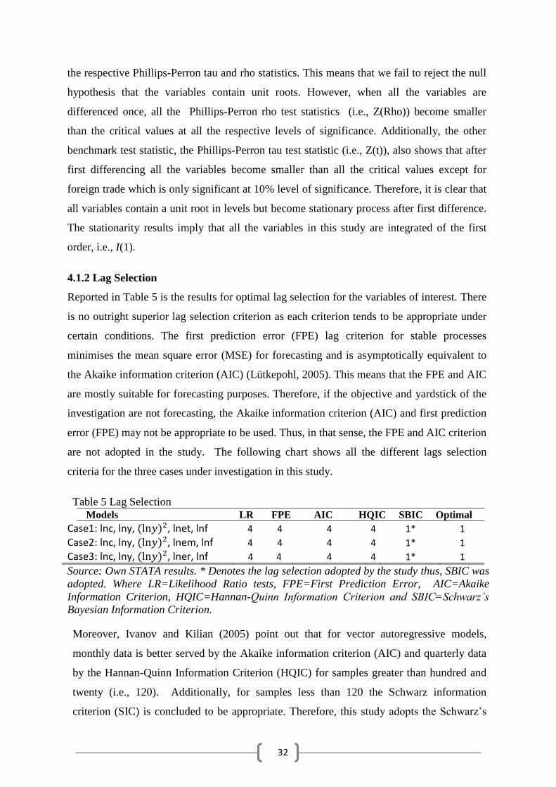
32
the respective Phillips-Perron tau and rho statistics. This means that we fail to reject the null
hypothesis that the variables contain unit roots. However, when all the variables are
differenced once, all the Phillips-Perron rho test statistics (i.e., Z(Rho)) become smaller
than the critical values at all the respective levels of significance. Additionally, the other
benchmark test statistic, the Phillips-Perron tau test statistic (i.e., Z(t)), also shows that after
first differencing all the variables become smaller than all the critical values except for
foreign trade which is only significant at 10% level of significance. Therefore, it is clear that
all variables contain a unit root in levels but become stationary process after first difference.
The stationarity results imply that all the variables in this study are integrated of the first
order, i.e., I(1).
4.1.2 Lag Selection
Reported in Table 5 is the results for optimal lag selection for the variables of interest. There
is no outright superior lag selection criterion as each criterion tends to be appropriate under
certain conditions. The first prediction error (FPE) lag criterion for stable processes
minimises the mean square error (MSE) for forecasting and is asymptotically equivalent to
the Akaike information criterion (AIC) (Lütkepohl, 2005). This means that the FPE and AIC
are mostly suitable for forecasting purposes. Therefore, if the objective and yardstick of the
investigation are not forecasting, the Akaike information criterion (AIC) and first prediction
error (FPE) may not be appropriate to be used. Thus, in that sense, the FPE and AIC criterion
are not adopted in the study. The following chart shows all the different lags selection
criteria for the three cases under investigation in this study.
Table 5 Lag Selection
Models LR FPE AIC HQIC SBIC Optimal
Case1: lnc, lny, (ln𝑦)2, lnet, lnf 4 4 4 4 1* 1
Case2: lnc, lny, (ln𝑦)2, lnem, lnf 4 4 4 4 1* 1
Case3: lnc, lny, (ln𝑦)2, lner, lnf 4 4 4 4 1* 1
Source: Own STATA results. * Denotes the lag selection adopted by the study thus, SBIC was
adopted. Where LR=Likelihood Ratio tests, FPE=First Prediction Error, AIC=Akaike
Information Criterion, HQIC=Hannan-Quinn Information Criterion and SBIC=Schwarz’s
Bayesian Information Criterion.
Moreover, Ivanov and Kilian (2005) point out that for vector autoregressive models,
monthly data is better served by the Akaike information criterion (AIC) and quarterly data
by the Hannan-Quinn Information Criterion (HQIC) for samples greater than hundred and
twenty (i.e., 120). Additionally, for samples less than 120 the Schwarz information
criterion (SIC) is concluded to be appropriate. Therefore, this study adopts the Schwarz’s
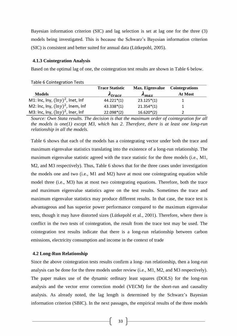
33
Bayesian information criterion (SIC) and lag selection is set at lag one for the three (3)
models being investigated. This is because the Schwarz’s Bayesian information criterion
(SIC) is consistent and better suited for annual data (Lütkepohl, 2005).
4.1.3 Cointegration Analysis
Based on the optimal lag of one, the cointegration test results are shown in Table 6 below.
Table 6 Cointegration Tests
Trace Statistic Max. Eigenvalue Cointegrations
Models 𝝀𝒕𝒓𝒂𝒄𝒆 𝝀𝒎𝒂𝒙 At Most
M1: lnc, lny, (ln𝑦)2, lnet, lnf 44.221*(1) 23.125*(1) 1
M2: lnc, lny, (ln𝑦)2, lnem, lnf 43.338*(1) 21.354*(1) 1
M3: lnc, lny, (ln𝑦)2, lner, lnf 22.098*(2) 16.620*(2) 2
Source: Own Stata results. The decision is that the maximum order of cointegration for all
the models is one(1) except M3, which has 2. Therefore, there is at least one long-run
relationship in all the models.
Table 6 shows that each of the models has a cointegrating vector under both the trace and
maximum eigenvalue statistics translating into the existence of a long-run relationship. The
maximum eigenvalue statistic agreed with the trace statistic for the three models (i.e., M1,
M2, and M3 respectively). Thus, Table 6 shows that for the three cases under investigation
the models one and two (i.e., M1 and M2) have at most one cointegrating equation while
model three (i.e., M3) has at most two cointegrating equations. Therefore, both the trace
and maximum eigenvalue statistics agree on the test results. Sometimes the trace and
maximum eigenvalue statistics may produce different results. In that case, the trace test is
advantageous and has superior power performance compared to the maximum eigenvalue
tests, though it may have distorted sizes (Lütkepohl et al., 2001). Therefore, where there is
conflict in the two tests of cointegration, the result from the trace test may be used. The
cointegration test results indicate that there is a long-run relationship between carbon
emissions, electricity consumption and income in the context of trade
4.2 Long-Run Relationship
Since the above cointegration tests results confirm a long- run relationship, then a long-run
analysis can be done for the three models under review (i.e., M1, M2, and M3 respectively).
The paper makes use of the dynamic ordinary least squares (DOLS) for the long-run
analysis and the vector error correction model (VECM) for the short-run and causality
analysis. As already noted, the lag length is determined by the Schwarz’s Bayesian
information criterion (SBIC). In the next passages, the empirical results of the three models
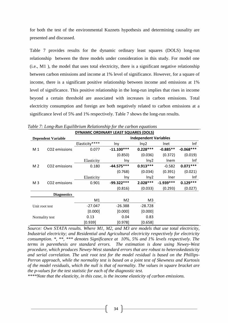
34
for both the test of the environmental Kuznets hypothesis and determining causality are
presented and discussed.
Table 7 provides results for the dynamic ordinary least squares (DOLS) long-run
relationship between the three models under consideration in this study. For model one
(i.e., M1 ), the model that uses total electricity, there is a significant negative relationship
between carbon emissions and income at 1% level of significance. However, for a square of
income, there is a significant positive relationship between income and emissions at 1%
level of significance. This positive relationship in the long-run implies that rises in income
beyond a certain threshold are associated with increases in carbon emissions. Total
electricity consumption and foreign are both negatively related to carbon emissions at a
significance level of 5% and 1% respectively. Table 7 shows the long-run results.
Table 7: Long-Run Equilibrium Relationship for the carbon equations DYNAMIC ORDINARY LEAST SQUARES (DOLS)
Dependent Variable Independent Variables
Elasticity**** lny lny2 lnet lnf
M 1 CO2 emissions 0.077 -11.100*** 0.228*** -0.885** -0.068***
(0.850) (0.036) (0.372) (0.019)
Elasticity lny lny2 lnem lnf
M 2 CO2 emissions 0.180 -44.575*** 0.913*** -0.582 0.071***
(0.768) (0.034) (0.391) (0.021)
Elasticity lny lny2 lner lnf
M 3 CO2 emissions 0.901 -99.322*** 2.028*** -1.939*** 0.129***
(0.816) (0.033) (0.293) (0.027)
Diagnostics
M1 M2 M3
Unit root test -27.047 -26.388 -28.728
[0.000] [0.000] [0.000]
Normality test 0.13 0.04 0.83
[0.939] [0.978] [0.658]
Source: Own STATA results. Where M1, M2, and M3 are models that use total electricity,
Industrial electricity; and Residential and Agricultural electricity respectively for electricity
consumption. *, **, *** denotes Significance at 10%, 5% and 1% levels respectively. The
terms in parenthesis are standard errors. The estimation is done using Newey-West
procedure, which produces Newey-West standard errors that are robust to heteroskedasticity
and serial correlation. The unit root test for the model residual is based on the Phillips-
Perron approach, while the normality test is based on a joint test of Skewness and Kurtosis
of the model residuals, which the null is that of normality. The values in square bracket are
the p-values for the test statistic for each of the diagnostic test.
****Note that the elasticity, in this case, is the income elasticity of carbon emissions.
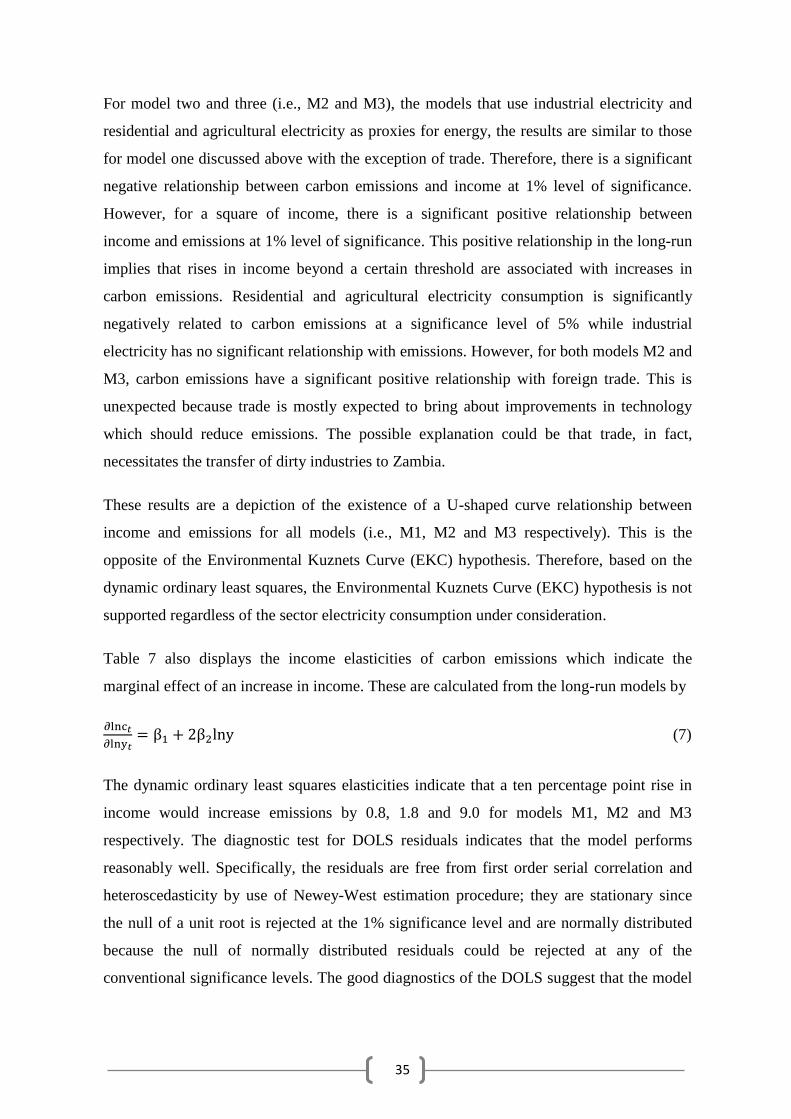
35
For model two and three (i.e., M2 and M3), the models that use industrial electricity and
residential and agricultural electricity as proxies for energy, the results are similar to those
for model one discussed above with the exception of trade. Therefore, there is a significant
negative relationship between carbon emissions and income at 1% level of significance.
However, for a square of income, there is a significant positive relationship between
income and emissions at 1% level of significance. This positive relationship in the long-run
implies that rises in income beyond a certain threshold are associated with increases in
carbon emissions. Residential and agricultural electricity consumption is significantly
negatively related to carbon emissions at a significance level of 5% while industrial
electricity has no significant relationship with emissions. However, for both models M2 and
M3, carbon emissions have a significant positive relationship with foreign trade. This is
unexpected because trade is mostly expected to bring about improvements in technology
which should reduce emissions. The possible explanation could be that trade, in fact,
necessitates the transfer of dirty industries to Zambia.
These results are a depiction of the existence of a U-shaped curve relationship between
income and emissions for all models (i.e., M1, M2 and M3 respectively). This is the
opposite of the Environmental Kuznets Curve (EKC) hypothesis. Therefore, based on the
dynamic ordinary least squares, the Environmental Kuznets Curve (EKC) hypothesis is not
supported regardless of the sector electricity consumption under consideration.
Table 7 also displays the income elasticities of carbon emissions which indicate the
marginal effect of an increase in income. These are calculated from the long-run models by
∂lnc𝑡
∂lny𝑡= β1 + 2β2lny (7)
The dynamic ordinary least squares elasticities indicate that a ten percentage point rise in
income would increase emissions by 0.8, 1.8 and 9.0 for models M1, M2 and M3
respectively. The diagnostic test for DOLS residuals indicates that the model performs
reasonably well. Specifically, the residuals are free from first order serial correlation and
heteroscedasticity by use of Newey-West estimation procedure; they are stationary since
the null of a unit root is rejected at the 1% significance level and are normally distributed
because the null of normally distributed residuals could be rejected at any of the
conventional significance levels. The good diagnostics of the DOLS suggest that the model
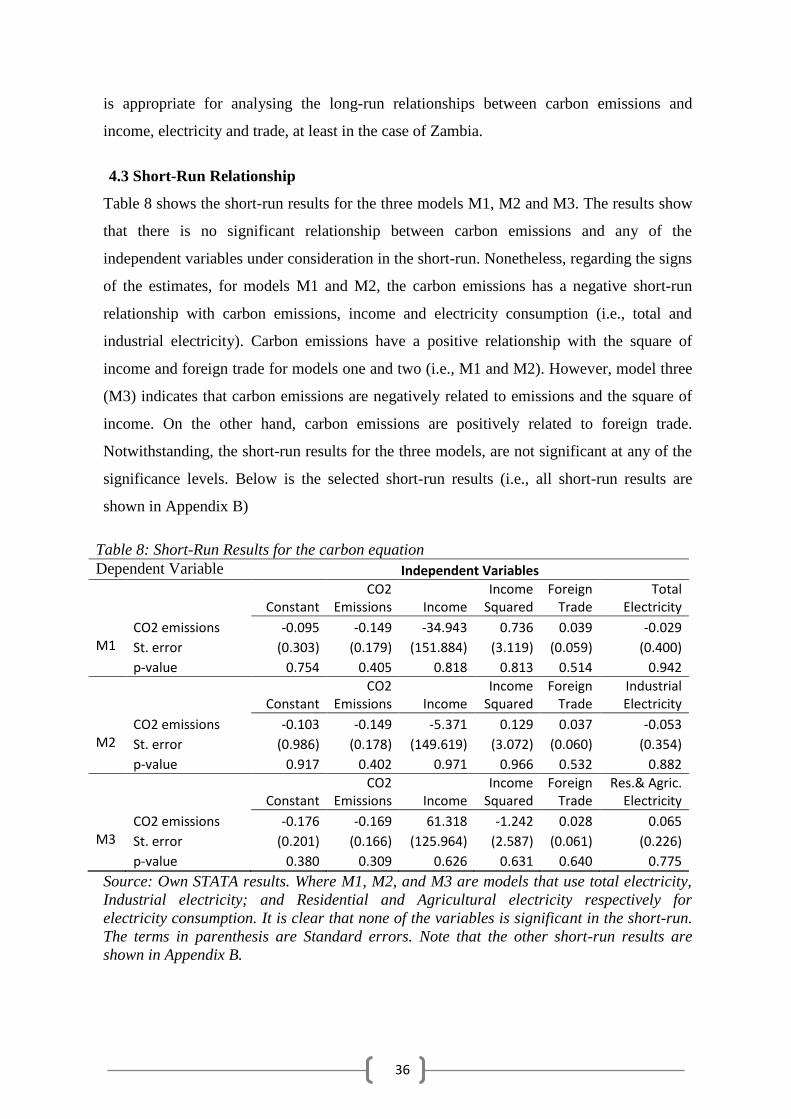
36
is appropriate for analysing the long-run relationships between carbon emissions and
income, electricity and trade, at least in the case of Zambia.
4.3 Short-Run Relationship
Table 8 shows the short-run results for the three models M1, M2 and M3. The results show
that there is no significant relationship between carbon emissions and any of the
independent variables under consideration in the short-run. Nonetheless, regarding the signs
of the estimates, for models M1 and M2, the carbon emissions has a negative short-run
relationship with carbon emissions, income and electricity consumption (i.e., total and
industrial electricity). Carbon emissions have a positive relationship with the square of
income and foreign trade for models one and two (i.e., M1 and M2). However, model three
(M3) indicates that carbon emissions are negatively related to emissions and the square of
income. On the other hand, carbon emissions are positively related to foreign trade.
Notwithstanding, the short-run results for the three models, are not significant at any of the
significance levels. Below is the selected short-run results (i.e., all short-run results are
shown in Appendix B)
Table 8: Short-Run Results for the carbon equation Dependent Variable Independent Variables
Constant CO2
Emissions Income Income
Squared Foreign
Trade Total
Electricity
CO2 emissions -0.095 -0.149 -34.943 0.736 0.039 -0.029 M1 St. error (0.303) (0.179) (151.884) (3.119) (0.059) (0.400) p-value 0.754 0.405 0.818 0.813 0.514 0.942
Constant
CO2 Emissions Income
Income Squared
Foreign Trade
Industrial Electricity
CO2 emissions -0.103 -0.149 -5.371 0.129 0.037 -0.053 M2 St. error (0.986) (0.178) (149.619) (3.072) (0.060) (0.354) p-value 0.917 0.402 0.971 0.966 0.532 0.882
Constant
CO2 Emissions Income
Income Squared
Foreign Trade
Res.& Agric. Electricity
CO2 emissions -0.176 -0.169 61.318 -1.242 0.028 0.065 M3 St. error (0.201) (0.166) (125.964) (2.587) (0.061) (0.226) p-value 0.380 0.309 0.626 0.631 0.640 0.775
Source: Own STATA results. Where M1, M2, and M3 are models that use total electricity,
Industrial electricity; and Residential and Agricultural electricity respectively for
electricity consumption. It is clear that none of the variables is significant in the short-run.
The terms in parenthesis are Standard errors. Note that the other short-run results are
shown in Appendix B.
37
The short-run model that gives these short-run results is based on the vector error correction
model discussed in section 3.2.4. Having established the existence of a long-run
relationship, the short-run results above indicate that it does not matter what energy policies
are put in place in the short-run, i.e., either energy conservation policies, growth policies or
a combination of both. This is because the results show that there is no short-run
relationship for all the cases under consideration (i.e., M1, M2 and M3). Therefore, from a
policy front, it should mostly be emphasised to be wary of what policies are implemented in
the long-run as for the short-run policies are thought of to have less consequence
detrimental consequences due to the insignificant short run relationships.
4.3.1 Results of Granger Causality
Finally, the empirical results in Table 9 show the Granger causality test results of the
observed relationships among the variables in the previous sections. The results in Table 9
indicates the direction of causality among the variables in question for the period between
1971 and 2010. The full set of the causality results are provided in Appendix C. The null
hypothesis in the tests below is that the respective lagged independent variables do not
cause dependent variables in question. Below are the Granger causality results.
Table 9 Short-Run and Long-Run Granger Causality 𝜒2 Results
Short-Run
CO2 lny lny2 lnf lnet
M1
CO2 Emissions (lnc)
0.050 0.060 0.430 0.010
(0.818) (0.813) (0.514) (0.942)
Electricity(lnet) 0.140 0.080 0.080 0.060
(0.709) (0.783) (0.781) (0.804)
CO2 lny lny2 lnf lnem
M2
CO2 Emissions (lnc)
0.000 0.000 0.390 0.020
(0.971) (0.966) (0.532) (0.882)
Electricity (lnem) 0.010 0.070 0.070 0.000
(0.941) (0.796) (0.797) (0.971)
CO2 lny lny2 lnf lner
M3
CO2 Emissions (lnc)
0.240 0.230 0.220 0.080
(0.626) (0.631) (0.640) (0.775)
Electricity (lner) 0.580 5.900* 5.920* 0.760
(0.445) (0.015) (0.015) (0.384)
Source: Own STATA results for Granger Causality. Note: The values in parenthesis are p-values.
M1, M2, and M3 represent the three estimated models. *, ** and *** denotes Significant at 10%,
5% and 1% levels of significance respectively. Appendix C shows all causality results
Summary of Causality:
Income → Residential & Agricultural Electricity
Income squared → Residential & Agricultural Electricity
38
For equation one (i.e., M1) none of the variables indicates a significant causality results on
carbon emissions. Thus, we fail to reject the null hypotheses of no causality for the
respective independent variables and conclude that none of the variables cause carbon
emissions under model one (M1). Similarly, model two (M2) results show that none of the
variables significantly causes carbon emissions, a similar conclusion as in model one (M1).
Additionally, with regards to causality to electricity consumption, none of the variables
Granger cause either the total or industrial electricity consumption.
On the other hand, the third model (M3) also shows that there is also no causality between
carbon emissions and the respective independent variables. However, there is evidence of
causality running from income to residential and agricultural electricity consumption at 5%
level of significance.
The causality of income on residential and agricultural electricity consumption is a one-way
causality or uni-directional causality. This means that income Granger cases residential and
agricultural electricity consumption without any feedback. Additionally, there are some
other causality results not indicated here6. Another important result of our study is that all
variables in models one, two and three (i.e., M1, M2, and M3) jointly cause foreign trade
respectively, all at 1% levels of significance. Moreover, for model three (M3) all variables
significantly Granger cause residential and agricultural electricity consumption.
4.4 Diagnostic Tests
4.4.1 Normality and Autocorrelation for the VECM
As a final step, we also check the model diagnostics to be sure the model reasonably
captures the data generating process. In this, we perform a Lagrange Multiplier test to
check for autocorrelation in the estimated models. The null hypothesis for the tests in Table
10 is that there is no autocorrelation, and the results are shown below leading to failure to
reject the null hypothesis in all the estimated models at the 5 % significance level.
6 More results are shown in Appendix C
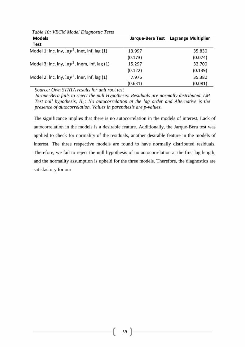
39
Table 10: VECM Model Diagnostic Tests Models Jarque-Bera Test Lagrange Multiplier Test
Model 1: lnc, lny, ln𝑦2, lnet, lnf, lag (1) 13.997 35.830
(0.173) (0.074)
Model 3: lnc, lny, ln𝑦2, lnem, lnf, lag (1) 15.297 32.700
(0.122) (0.139)
Model 2: lnc, lny, ln𝑦2, lner, lnf, lag (1) 7.976 35.380
(0.631) (0.081)
Source: Own STATA results for unit root test
Jarque-Bera fails to reject the null Hypothesis: Residuals are normally distributed. LM
Test null hypothesis, 𝐻0: No autocorrelation at the lag order and Alternative is the
presence of autocorrelation. Values in parenthesis are p-values.
The significance implies that there is no autocorrelation in the models of interest. Lack of
autocorrelation in the models is a desirable feature. Additionally, the Jarque-Bera test was
applied to check for normality of the residuals, another desirable feature in the models of
interest. The three respective models are found to have normally distributed residuals.
Therefore, we fail to reject the null hypothesis of no autocorrelation at the first lag length,
and the normality assumption is upheld for the three models. Therefore, the diagnostics are
satisfactory for our
40
5.0 Policy Analysis and Conclusion
This paper examines both the testing of the environmental Kuznets curve (EKC) hypothesis
and causality test analysis. The cointegration analysis done in this study concludes a
presence of long-run relationships in the three models under consideration7. The long-run
relationship is found among the variables under consideration, i.e., carbon emissions,
electricity use, foreign trade and income.
By the dynamic ordinary least squares in the long-run models, it was found that there is no
evidence in support of the Environmental Kuznets Curve (EKC) hypothesis. Nonetheless,
what is instead concluded is that there is an opposite of the environmental Kuznets curve
(EKC), in that we find a U-shaped curve relationship between income and carbon emission.
The implication is that in the long-run income growth initially reduces carbon emissions
but beyond a certain threshold the carbon emissions are expected to rise. A possible reason
could be that income levels are low to start with, implying more reliability on production
and consumptions patterns that generate fewer carbon emissions, but as income level
increases, both production and consumption patterns tend to shift towards more carbon-
intensive production and consumption patterns.
The conclusion on causality is that there is evidence of no causality between either total
electricity and income or between industrial electricity and income in the short-run.
Therefore, in the short-run, there is evidence of a neutrality hypothesis between total
electricity consumption and income and also between industrial electricity consumption
and income. This means that for models M1 and M2 there is no causality between income
and electricity consumption.
The policy implications of the above two results are that policymakers can institute either
conservation or growth policies in the industrial sector or on overall for the whole economy
(i.e., total electricity use) without significantly affecting national income. On the other
hand, a different result is obtained for the third model. Thus, there is evidence of income
Granger causing residential and agricultural electricity consumption without feedback in a
model that uses residential and agricultural electricity. This is evidence of the conservation
hypothesis, in which electricity consumption is growth led. In this scenario, disruptions in
7 M1, M2 and M3 use total electricity, industrial electricity and residential and agricultural
electricity and proxies for energy respectively.
41
growth would have an impact on residential and agricultural electricity consumption. This
is particularly, important for policy analysis because only conservation policies can be
undertaken on residential and agricultural without affecting national income.
5.2 Possible Areas for further research and Limitations
Several areas for possible further research are available on this theme of energy economics.
Firstly, the study can be broadened further by considering testing for other pollutants such
as sulphur, nitrous oxide, volatile organic compounds (VOC), etc. It is argued that
Environmental Kuznets Curve (EKC) hypothesis applies to problems that are easy to solve
and are well known and documented (Dinda, 2004).
Another area that is ripe for policy relevant research is the checking of the impact of
electricity consumption on cyclical fluctuation or business cycles. It is argued that
application of the Hodrix-Prescott (HP) filter decomposes the trend, and cyclical
components and thereby provides a stronger result than mere cointegration (Akinlo, 2009).
This is an interesting field for further research. Lastly, an interesting area for further
research would be the investigation of causality and analysis of the Environmental Kuznets
Curve (EKC) hypothesis in the context of value added by the specific industries as opposed
to the use of the overall gross domestic product. In a similar vein, there is room for further
research with regards to the impact of structural breaks arising from power sector reforms.
Certain points impede the validity of the Environmental Kuznets Curve (EKC) hypothesis
such as whether it is a permanent phenomenon, valid for individual countries and the
world, valid for all environmental pressures or whether it follows a sustainable
development path (Dinda, 2004). This study only checks the validity of the environmental
Kuznets curve (EKC) hypothesis for Zambia and does not delve into testing for most
pollutants apart from carbon emissions. Additionally, the paper does not attempt to confirm
if the Environmental Kuznets Curve (EKC) hypothesis is permanent or follows a
sustainable development path.

42
References
Akinlo, A.E., 2009. Electricity consumption and economic growth in Nigeria: Evidence from cointegration and co-feature analysis. J. Policy Model. 31, 681–693. doi:10.1016/j.jpolmod.2009.03.004
Akpan, G.E., Akpan, U.F., 2012. Electricity consumption, carbon emissions and economic growth in Nigeria. Int. J. Energy Econ. Policy 2, 292.
Al-Azzam, A., Hawdon, D., 1999. Estimating the demand for energy in Jordan: a Stock-Watson dynamic OLS (DOLS) approach, Surrey energy economics discussion paper series. Surrey Energy Economics Centre, Guildford.
Alkhathlan, K., Javid, M., 2013. Energy consumption, carbon emissions and economic growth in Saudi Arabia: An aggregate and disaggregate analysis. Energy Policy 62, 1525–1532. doi:10.1016/j.enpol.2013.07.068
Al-Mulali, U., Ozturk, I., Solarin, S.A., 2016. Investigating the environmental Kuznets curve hypothesis in seven regions: The role of renewable energy. Ecol. Indic. 67, 267–282. doi:10.1016/j.ecolind.2016.02.059
Ankarhem, M., 2005. A Dual Assessment of the Environmental Kuznets Curve: The Case of Sweden (No. 660). Umeå University, Department of Economics, Umeå, Sweden.
Baek, J., 2015. Environmental Kuznets curve for CO2 emissions: The case of Arctic countries. Energy Econ. 50, 13–17. doi:10.1016/j.eneco.2015.04.010
Baek, J., Cho, Y., Koo, W.W., 2009. The environmental consequences of globalisation: A country-specific time-series analysis. Ecol. Econ. 68, 2255–2264. doi:10.1016/j.ecolecon.2009.02.021
Begum, R.A., Sohag, K., Abdullah, S.M.S., Jaafar, M., 2015. CO2 emissions, energy consumption, economic and population growth in Malaysia. Renew. Sustain. Energy Rev. 41, 594–601. doi:10.1016/j.rser.2014.07.205
Bhattacharyya, S.C., 2011. Energy Economics. Springer London, London. Bildirici, M.E., 2013. The Analysis of Relationship Between Economic Growth and Electricity
Consumption in Africa by ARDL Method. Energy Econ. Lett. 1, 1–14. Brock, W.A., Taylor, M.S., 2010. The Green Solow model. J. Econ. Growth 15, 127–153.
doi:10.1007/s10887-010-9051-0 Camacho-Gutiérrez, P., 2010. Dynamic OLS estimation of the US import demand for Mexican crude
oil. Central Statistical Office (CSO) [Zambia], Ministry of Health (MOH) [Zambia], and ICF International.
2014, 2015. Zambia Demographic and Health Survey 2013-14 , and ICF International., : (Survey). Central Statistical Office (CSO), Ministry of Health (MoH), Rockville, Maryland, USA.
Chandran, V.G.R., Sharma, S., Madhavan, K., 2010. Electricity consumption–growth nexus: The case of Malaysia. Energy Policy 38, 606–612. doi:10.1016/j.enpol.2009.10.013
Copeland, B.R., Taylor, M.S., 1995. Trade and the Environment: A Partial Synthesis. Am. J. Agric. Econ. 77, 765–771.
CSO, 2007. Environmental Statistics in Zambia: Energy Statistics. Central Statistical Office (CSO), Lusaka, Zambia.
Dinda, S., 2004. Environmental Kuznets Curve Hypothesis: A Survey. Ecol. Econ. 49, 431–455. doi:10.1016/j.ecolecon.2004.02.011
Energy Regulation Board, n.d. Energy Regulation Board (ERB), 2015. , Energy Sector Report 2014. Energy Regulation Board (ERB). Engle, R.., Granger, C.W.J., 1987. Co-Integration and Error Correction: Representation, Estimation,
and Testing. Econometrica 55. Ghosh, S., 2002. Electricity consumption and economic growth in India. Energy Policy 30, 125–129. Granger, C.W., Newbold, P., 1974. Spurious regressions in econometrics. J. Econom. 2, 111–120. Gujarati, D.N., Porter, D.C., 2009. Basic econometrics, 5th ed. ed. McGraw-Hill Irwin, Boston. International Energy Agency, n.d.
43
Ivanov, V., Kilian, L., 2005. A practitioner’s guide to lag order selection for VAR impulse response analysis. Stud. Nonlinear Dyn. Econom. 9.
Johansson, P.-O., Kriström, B., 2007. On a clear day, you might see an environmental Kuznets curve. Environ. Resour. Econ. 37, 77–90. doi:10.1007/s10640-007-9112-9
Joskow, P.L., 2008. Lessons learned from electricity market liberalisation. Energy J. 29, 9–42. Jumbe, C.B., 2004. Cointegration and causality between electricity consumption and GDP: empirical
evidence from Malawi. Energy Econ. 26, 61–68. Kohler, M., 2013. CO2 emissions, energy consumption, income and foreign trade: A South African
perspective. Energy Policy 63, 1042–1050. doi:10.1016/j.enpol.2013.09.022 Kouakou, A.K., 2011. Economic growth and electricity consumption in Cote d’Ivoire: Evidence from
time series analysis. Energy Policy 39, 3638–3644. doi:10.1016/j.enpol.2011.03.069 Lütkepohl, H., 2005. A new introduction to multiple time series analysis. New York : Springer, Berlin. Lütkepohl, H., Saikkonen, P., Trenkler, C., 2001. Maximum eigenvalue versus trace tests for the
cointegrating rank of a VAR process. Economy. J. 4, 287–310. Machungwa, P.., 2005. Paper on Zambia’s Experience with Power Sector Reform, in Parliamentary
Reform on Energy Legislation and Sustainable Development. Cape Town, South Africa, pp. 1–14.
Mankiw, N.G., 2009. Macroeconomics, 7th ed. ed. Worth Publishers, New York, NY. Mendonça, A.F., Dahl, C., 1999. The Brazilian electrical system reform. Energy Policy 27, 73–83. Mensah, J.T., 2014. Carbon emissions, energy consumption and output: A threshold analysis on the
causal dynamics in emerging African economies. Energy Policy 70, 172–182. doi:10.1016/j.enpol.2014.03.038
Moyo, E., Pokhrel, B.R., Adhikary, B., 2015. Modelling and Analysis of Wholesale Competitive Electricity Markets: A Case For Zambia. IJERA 5, pp.07-12.
Odhiambo, N.M., 2009. Electricity consumption and economic growth in South Africa: A trivariate causality test. Energy Econ. 31, 635–640. doi:10.1016/j.eneco.2009.01.005
Ouédraogo, I.M., 2010. Electricity consumption and economic growth in Burkina Faso: A cointegration analysis. Energy Econ. 32, 524–531. doi:10.1016/j.eneco.2009.08.011
Ozturk, I., 2010. A literature survey on energy–growth nexus. Energy Policy 38, 340–349. doi:10.1016/j.enpol.2009.09.024
Perman, R., Perman, R. (Eds.), 2011. Natural resource and environmental economics, 4th ed. ed. Pearson Addison Wesley, Harlow, Essex ; New York.
Romer, D., 1996. Advanced macroeconomics, McGraw-Hill advanced series in economics. McGraw-Hill Companies, New York.
Saboori, B., Sulaiman, J., 2013. Environmental degradation, economic growth and energy consumption: Evidence of the environmental Kuznets curve in Malaysia. Energy Policy 60, 892–905. doi:10.1016/j.enpol.2013.05.099
Shahbaz, M., Lean, H.H., 2012. The dynamics of electricity consumption and economic growth: A revisit study of their causality in Pakistan. Energy 39, 146–153. doi:10.1016/j.energy.2012.01.048
Shahbaz, M., Tang, C.F., Shahbaz Shabbir, M., 2011. Electricity consumption and economic growth nexus in Portugal using cointegration and causality approaches. Energy Policy 39, 3529–3536. doi:10.1016/j.enpol.2011.03.052
Shiu, A., Lam, P.-L., 2004. Electricity consumption and economic growth in China. Energy Policy 32, 47–54.
Stefanski, R., 2013. OxCarre Research Paper 47. Vagliasindi, M., Besant-Jones, J., 2013. Power market structure: revisiting policy options. The World
Bank, Washington, D.C. Wolde-Rufael, Y., 2006. Electricity consumption and economic growth: a time series experience for
17 African countries. Energy Policy 34, 1106–1114. doi:10.1016/j.enpol.2004.10.008

44
World Bank, 2002. The World Bank’s Poverty Reduction Strategy Paper and Joint Staff Assessment (Poverty Reduction Strategy Paper and Joint Staff Assessment No. Report No: 24035-ZA). Prepared by Staffs of the International Development Association and the International Monetary Fund.
World Bank (Ed.), 1992. Development and the environment, World development indicators. Oxford Univ. Press, Oxford.
World Bank, n.d. CO2 emissions (metric tonnes per capita). World Bank, n.d. GDP at market prices (constant 2005 US$). Zambia Development Agency (ZDA), 2014. , Energy Sector Profile. Zambia Development Agency
(ZDA). Zambia Electricity Supply Corporation, n.d.
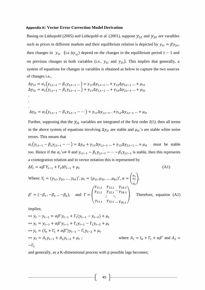
45
Appendix A: Vector Error Correction Model Derivation
Basing on Lütkepohl (2005) and Lütkepohl et al. (2001), suppose 𝑦1𝑡 and 𝑦2𝑡 are varaibles
such as prices in different markets and their equilibrium relation is depicted by 𝑦1𝑡 = 𝛽𝑦2𝑡,
then changes in 𝑦1𝑡 (i.e ∆𝑦1𝑡) depend on the changes in the equilibrium period 𝑡 − 1 and
on previous chnages in both variables (i.e., 𝑦1𝑡 and 𝑦2𝑡). This implies that generally, a
system of equations for changes in variables is obtained as below to capture the two sources
of changes i.e.,
∆𝑦1𝑡 = 𝛼1(𝑦1,𝑡−1 − 𝛽1𝑦2,𝑡−1…) + 𝛾11∆𝑦1,𝑡−1…+ 𝛾12∆𝑦2,𝑡−1…+ 𝜇1𝑡
∆𝑦2𝑡 = 𝛼2(𝑦1,𝑡−1 − 𝛽1𝑦2,𝑡−1…) + 𝛾11∆𝑦1,𝑡−1…+ 𝛾12∆𝑦2,𝑡−1…+ 𝜇2𝑡
.
.
. ∆𝑦𝑖𝑡 = 𝛼𝑖(𝑦1,𝑡−1 − 𝛽1𝑦2,𝑡−1 −⋯) + 𝛾11∆𝑦1,𝑡−1. . +𝛾12∆𝑦2,𝑡−1…+ 𝜇𝑖𝑡
Further, supposing that the 𝑦𝑖𝑡 variables are integrated of the first order I(1), then all terms
in the above system of equations involving ∆𝑦𝑖𝑡 are stable and 𝜇𝑖𝑡’s are stable white noise
errors. This means that
𝛼𝑖(𝑦𝑖,𝑡−1 − 𝛽1𝑦𝑗,𝑡−1 −⋯) = ∆𝑦𝑖𝑡 + 𝛾11∆𝑦1,𝑡−1…+ 𝛾12∆𝑦2,𝑡−1…+ 𝜇𝑖𝑡 must be stable
too. Hence if the 𝛼𝑖’s≠ 0 and 𝑦𝑖,𝑡−1 − 𝛽1𝑦𝑗,𝑡−1 −⋯−𝛽1𝑦𝑗,𝑡−1 is stable, then this represents
a cointegration relation and in vector notation this is represented by
∆𝑌𝑡 = 𝛼𝛽′𝑌𝑡−1 + Γ1∆𝑌𝑡−1 + 𝜇𝑡 (A1)
Where: 𝑌𝑡 = (𝑦1𝑡, 𝑦2𝑡, … , 𝑦𝑘𝑡)′, 𝜇𝑡 = (𝜇1𝑡, 𝜇2𝑡, … , 𝜇𝑘𝑡)′, 𝛼 = (𝛼1𝛼2:𝛼𝑡
),
𝛽′ = (−𝛽1 , −𝛽2…−𝛽𝑘), and Γ = (
𝛾11,1 𝛾12,1𝛾21,1 𝛾22,1
…𝛾1𝑘,1𝛾2𝑘,1
⋮ ⋱𝛾𝑡1,1 𝛾𝑡2,1…𝛾𝑡𝑘,1
). Therefore, equation (A1)
implies;
↔ 𝑦𝑡 − 𝑦𝑡−1 = 𝛼𝛽′𝑦𝑡−1 + Γ1(𝑦𝑡−1 − 𝑦𝑡−2) + 𝜇𝑡
↔ 𝑦𝑡 = 𝑦𝑡−1 + 𝛼𝛽′𝑦𝑡−1 + Γ1𝑦𝑡−1 − Γ1𝑦𝑡−2 + 𝜇𝑡
↔ 𝑦𝑡 = (𝐼𝑘 + Γ1 + 𝛼𝛽′)𝑦𝑡−1 − Γ1𝑦𝑡−2 + 𝜇𝑡
↔ 𝑦𝑡 = 𝐴1𝑦𝑡−1 + 𝐴2𝑦𝑡−2 + 𝜇𝑡 ; where 𝐴1 = 𝐼𝑘 + Γ1 + 𝛼𝛽′ and 𝐴2 =
−Γ1
and generally, as a K-dimensional process with p possible lags becomes;
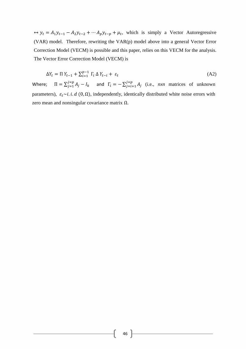
46
↔ 𝑦𝑡 = 𝐴1𝑦𝑡−1 − 𝐴2𝑦𝑡−2 +⋯𝐴𝑝𝑦𝑡−𝑝 + 𝜇𝑡, which is simply a Vector Autoregressive
(VAR) model. Therefore, rewriting the VAR(p) model above into a general Vector Error
Correction Model (VECM) is possible and this paper, relies on this VECM for the analysis.
The Vector Error Correction Model (VECM) is
∆𝑌𝑡 = Π 𝑌𝑡−1 + ∑ Γ𝑖 Δ 𝑌𝑡−𝑖𝑝−1𝑖=1 + 휀𝑡 (A2)
Where; Π = ∑ 𝐴𝑗 − 𝐼𝑘𝑗=𝑝𝑗=1 and Γ𝑖 = −∑ 𝐴𝑗
𝑗=𝑝𝑗=𝑖+1 (i.e., nxn matrices of unknown
parameters), 휀𝑡~𝑖. 𝑖. 𝑑 (0, Ω), independently, identically distributed white noise errors with
zero mean and nonsingular covariance matrix Ω.
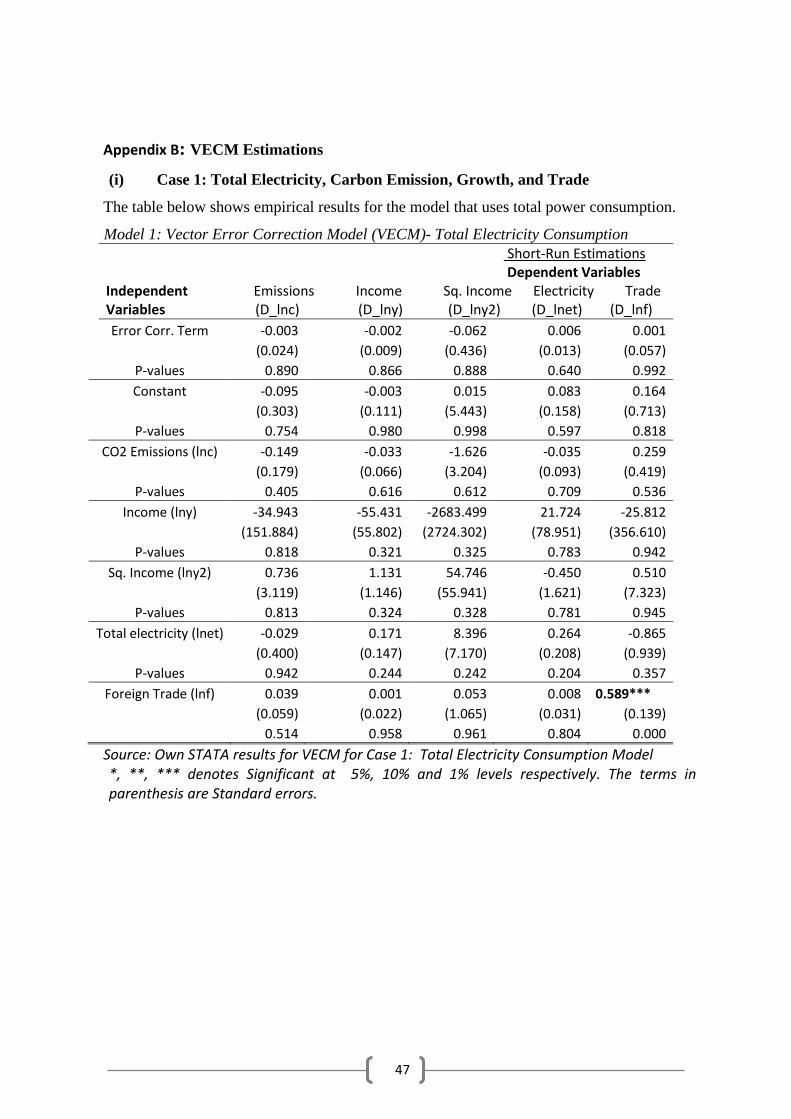
47
Appendix B: VECM Estimations
(i) Case 1: Total Electricity, Carbon Emission, Growth, and Trade
The table below shows empirical results for the model that uses total power consumption.
Model 1: Vector Error Correction Model (VECM)- Total Electricity Consumption Short-Run Estimations Dependent Variables Independent Emissions Income Sq. Income Electricity Trade Variables (D_lnc) (D_lny) (D_lny2) (D_lnet) (D_lnf)
Error Corr. Term -0.003 -0.002 -0.062 0.006 0.001
(0.024) (0.009) (0.436) (0.013) (0.057)
P-values 0.890 0.866 0.888 0.640 0.992
Constant -0.095 -0.003 0.015 0.083 0.164
(0.303) (0.111) (5.443) (0.158) (0.713)
P-values 0.754 0.980 0.998 0.597 0.818
CO2 Emissions (lnc) -0.149 -0.033 -1.626 -0.035 0.259
(0.179) (0.066) (3.204) (0.093) (0.419)
P-values 0.405 0.616 0.612 0.709 0.536
Income (lny) -34.943 -55.431 -2683.499 21.724 -25.812
(151.884) (55.802) (2724.302) (78.951) (356.610)
P-values 0.818 0.321 0.325 0.783 0.942
Sq. Income (lny2) 0.736 1.131 54.746 -0.450 0.510
(3.119) (1.146) (55.941) (1.621) (7.323)
P-values 0.813 0.324 0.328 0.781 0.945
Total electricity (lnet) -0.029 0.171 8.396 0.264 -0.865
(0.400) (0.147) (7.170) (0.208) (0.939)
P-values 0.942 0.244 0.242 0.204 0.357
Foreign Trade (lnf) 0.039 0.001 0.053 0.008 0.589***
(0.059) (0.022) (1.065) (0.031) (0.139)
0.514 0.958 0.961 0.804 0.000
Source: Own STATA results for VECM for Case 1: Total Electricity Consumption Model *, **, *** denotes Significant at 5%, 10% and 1% levels respectively. The terms in parenthesis are Standard errors.
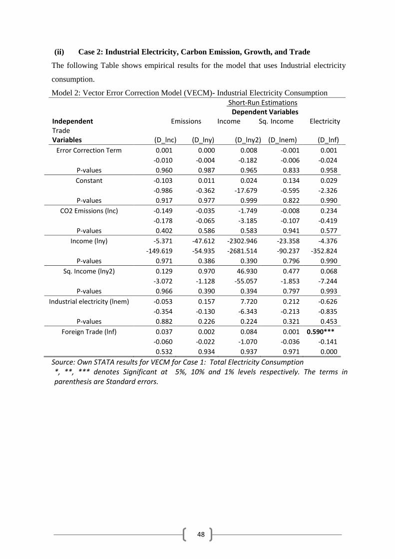
48
(ii) Case 2: Industrial Electricity, Carbon Emission, Growth, and Trade
The following Table shows empirical results for the model that uses Industrial electricity
consumption.
Model 2: Vector Error Correction Model (VECM)- Industrial Electricity Consumption
Short-Run Estimations Dependent Variables Independent Emissions Income Sq. Income Electricity Trade Variables (D_lnc) (D_lny) (D_lny2) (D_lnem) (D_lnf)
Error Correction Term 0.001 0.000 0.008 -0.001 0.001
-0.010 -0.004 -0.182 -0.006 -0.024
P-values 0.960 0.987 0.965 0.833 0.958
Constant -0.103 0.011 0.024 0.134 0.029
-0.986 -0.362 -17.679 -0.595 -2.326
P-values 0.917 0.977 0.999 0.822 0.990
CO2 Emissions (lnc) -0.149 -0.035 -1.749 -0.008 0.234
-0.178 -0.065 -3.185 -0.107 -0.419
P-values 0.402 0.586 0.583 0.941 0.577
Income (lny) -5.371 -47.612 -2302.946 -23.358 -4.376
-149.619 -54.935 -2681.514 -90.237 -352.824
P-values 0.971 0.386 0.390 0.796 0.990
Sq. Income (lny2) 0.129 0.970 46.930 0.477 0.068
-3.072 -1.128 -55.057 -1.853 -7.244
P-values 0.966 0.390 0.394 0.797 0.993
Industrial electricity (lnem) -0.053 0.157 7.720 0.212 -0.626
-0.354 -0.130 -6.343 -0.213 -0.835
P-values 0.882 0.226 0.224 0.321 0.453
Foreign Trade (lnf) 0.037 0.002 0.084 0.001 0.590***
-0.060 -0.022 -1.070 -0.036 -0.141
0.532 0.934 0.937 0.971 0.000
Source: Own STATA results for VECM for Case 1: Total Electricity Consumption *, **, *** denotes Significant at 5%, 10% and 1% levels respectively. The terms in parenthesis are Standard errors.
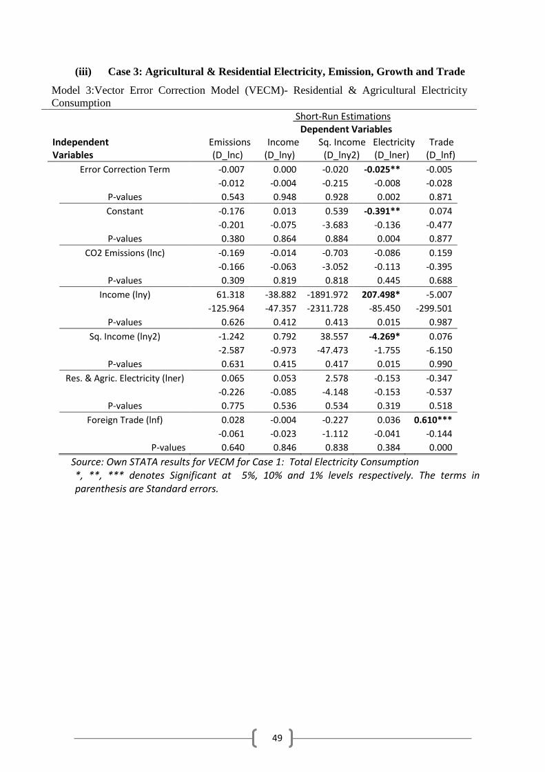
49
(iii) Case 3: Agricultural & Residential Electricity, Emission, Growth and Trade
Model 3:Vector Error Correction Model (VECM)- Residential & Agricultural Electricity
Consumption
Short-Run Estimations Dependent Variables Independent Emissions Income Sq. Income Electricity Trade Variables (D_lnc) (D_lny) (D_lny2) (D_lner) (D_lnf)
Error Correction Term -0.007 0.000 -0.020 -0.025** -0.005
-0.012 -0.004 -0.215 -0.008 -0.028
P-values 0.543 0.948 0.928 0.002 0.871
Constant -0.176 0.013 0.539 -0.391** 0.074
-0.201 -0.075 -3.683 -0.136 -0.477
P-values 0.380 0.864 0.884 0.004 0.877
CO2 Emissions (lnc) -0.169 -0.014 -0.703 -0.086 0.159
-0.166 -0.063 -3.052 -0.113 -0.395
P-values 0.309 0.819 0.818 0.445 0.688
Income (lny) 61.318 -38.882 -1891.972 207.498* -5.007
-125.964 -47.357 -2311.728 -85.450 -299.501
P-values 0.626 0.412 0.413 0.015 0.987
Sq. Income (lny2) -1.242 0.792 38.557 -4.269* 0.076
-2.587 -0.973 -47.473 -1.755 -6.150
P-values 0.631 0.415 0.417 0.015 0.990
Res. & Agric. Electricity (lner) 0.065 0.053 2.578 -0.153 -0.347
-0.226 -0.085 -4.148 -0.153 -0.537
P-values 0.775 0.536 0.534 0.319 0.518
Foreign Trade (lnf) 0.028 -0.004 -0.227 0.036 0.610***
-0.061 -0.023 -1.112 -0.041 -0.144
P-values 0.640 0.846 0.838 0.384 0.000
Source: Own STATA results for VECM for Case 1: Total Electricity Consumption *, **, *** denotes Significant at 5%, 10% and 1% levels respectively. The terms in parenthesis are Standard errors.
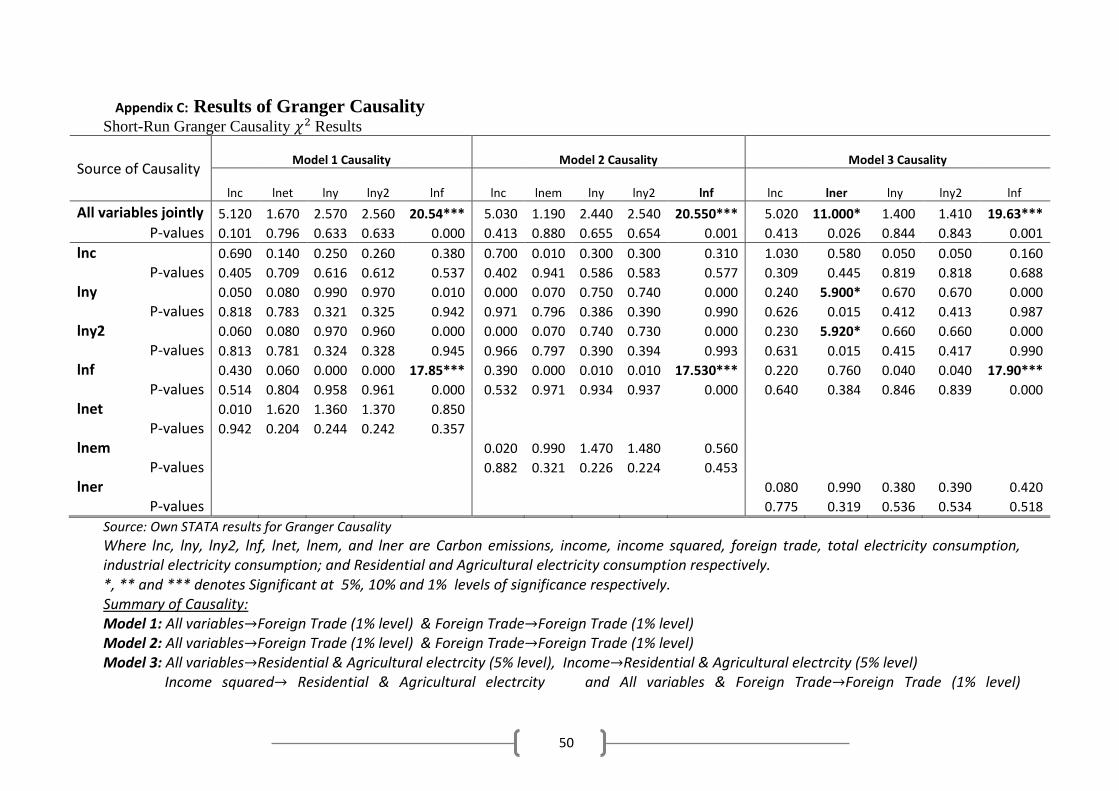
50
Appendix C: Results of Granger Causality
Short-Run Granger Causality 𝜒2 Results
Source of Causality Model 1 Causality Model 2 Causality Model 3 Causality
lnc lnet lny lny2 lnf
lnc lnem lny lny2 lnf lnc lner lny lny2 lnf
All variables jointly 5.120 1.670 2.570 2.560 20.54*** 5.030 1.190 2.440 2.540 20.550*** 5.020 11.000* 1.400 1.410 19.63***
P-values 0.101 0.796 0.633 0.633 0.000 0.413 0.880 0.655 0.654 0.001 0.413 0.026 0.844 0.843 0.001
lnc 0.690 0.140 0.250 0.260 0.380 0.700 0.010 0.300 0.300 0.310 1.030 0.580 0.050 0.050 0.160
P-values 0.405 0.709 0.616 0.612 0.537 0.402 0.941 0.586 0.583 0.577 0.309 0.445 0.819 0.818 0.688
lny 0.050 0.080 0.990 0.970 0.010 0.000 0.070 0.750 0.740 0.000 0.240 5.900* 0.670 0.670 0.000
P-values 0.818 0.783 0.321 0.325 0.942 0.971 0.796 0.386 0.390 0.990 0.626 0.015 0.412 0.413 0.987
lny2 0.060 0.080 0.970 0.960 0.000 0.000 0.070 0.740 0.730 0.000 0.230 5.920* 0.660 0.660 0.000
P-values 0.813 0.781 0.324 0.328 0.945 0.966 0.797 0.390 0.394 0.993 0.631 0.015 0.415 0.417 0.990
lnf 0.430 0.060 0.000 0.000 17.85*** 0.390 0.000 0.010 0.010 17.530*** 0.220 0.760 0.040 0.040 17.90***
P-values 0.514 0.804 0.958 0.961 0.000 0.532 0.971 0.934 0.937 0.000 0.640 0.384 0.846 0.839 0.000
lnet 0.010 1.620 1.360 1.370 0.850 P-values 0.942 0.204 0.244 0.242 0.357 lnem
0.020 0.990 1.470 1.480 0.560 P-values
0.882 0.321 0.226 0.224 0.453 lner
0.080 0.990 0.380 0.390 0.420
P-values
0.775 0.319 0.536 0.534 0.518
Source: Own STATA results for Granger Causality
Where lnc, lny, lny2, lnf, lnet, lnem, and lner are Carbon emissions, income, income squared, foreign trade, total electricity consumption, industrial electricity consumption; and Residential and Agricultural electricity consumption respectively. *, ** and *** denotes Significant at 5%, 10% and 1% levels of significance respectively. Summary of Causality: Model 1: All variables→Foreign Trade (1% level) & Foreign Trade→Foreign Trade (1% level) Model 2: All variables→Foreign Trade (1% level) & Foreign Trade→Foreign Trade (1% level) Model 3: All variables→Residential & Agricultural electrcity (5% level), Income→Residential & Agricultural electrcity (5% level) Income squared→ Residential & Agricultural electrcity and All variables & Foreign Trade→Foreign Trade (1% level)
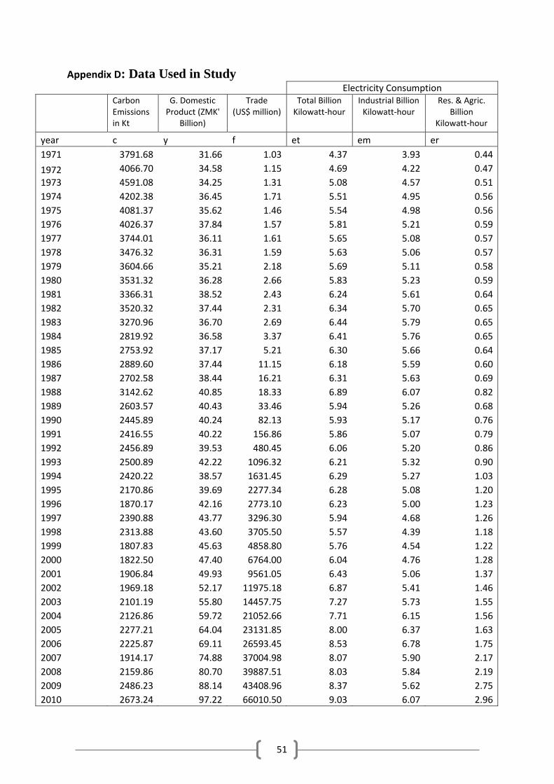
51
Appendix D: Data Used in Study Electricity Consumption
Carbon Emissions in Kt
G. Domestic Product (ZMK'
Billion)
Trade (US$ million)
Total Billion Kilowatt-hour
Industrial Billion Kilowatt-hour
Res. & Agric. Billion
Kilowatt-hour
year c y f et em er
1971 3791.68 31.66 1.03 4.37 3.93 0.44
1972 1973
4066.70 34.58 1.15 4.69 4.22 0.47
4591.08 34.25 1.31 5.08 4.57 0.51
1974 4202.38 36.45 1.71 5.51 4.95 0.56
1975 4081.37 35.62 1.46 5.54 4.98 0.56
1976 4026.37 37.84 1.57 5.81 5.21 0.59
1977 3744.01 36.11 1.61 5.65 5.08 0.57
1978 3476.32 36.31 1.59 5.63 5.06 0.57
1979 3604.66 35.21 2.18 5.69 5.11 0.58
1980 3531.32 36.28 2.66 5.83 5.23 0.59
1981 3366.31 38.52 2.43 6.24 5.61 0.64
1982 3520.32 37.44 2.31 6.34 5.70 0.65
1983 3270.96 36.70 2.69 6.44 5.79 0.65
1984 2819.92 36.58 3.37 6.41 5.76 0.65
1985 2753.92 37.17 5.21 6.30 5.66 0.64
1986 2889.60 37.44 11.15 6.18 5.59 0.60
1987 2702.58 38.44 16.21 6.31 5.63 0.69
1988 3142.62 40.85 18.33 6.89 6.07 0.82
1989 2603.57 40.43 33.46 5.94 5.26 0.68
1990 2445.89 40.24 82.13 5.93 5.17 0.76
1991 2416.55 40.22 156.86 5.86 5.07 0.79
1992 2456.89 39.53 480.45 6.06 5.20 0.86
1993 2500.89 42.22 1096.32 6.21 5.32 0.90
1994 2420.22 38.57 1631.45 6.29 5.27 1.03
1995 2170.86 39.69 2277.34 6.28 5.08 1.20
1996 1870.17 42.16 2773.10 6.23 5.00 1.23
1997 2390.88 43.77 3296.30 5.94 4.68 1.26
1998 2313.88 43.60 3705.50 5.57 4.39 1.18
1999 1807.83 45.63 4858.80 5.76 4.54 1.22
2000 1822.50 47.40 6764.00 6.04 4.76 1.28
2001 1906.84 49.93 9561.05 6.43 5.06 1.37
2002 1969.18 52.17 11975.18 6.87 5.41 1.46
2003 2101.19 55.80 14457.75 7.27 5.73 1.55
2004 2126.86 59.72 21052.66 7.71 6.15 1.56
2005 2277.21 64.04 23131.85 8.00 6.37 1.63
2006 2225.87 69.11 26593.45 8.53 6.78 1.75
2007 1914.17 74.88 37004.98 8.07 5.90 2.17
2008 2159.86 80.70 39887.51 8.03 5.84 2.19
2009 2486.23 88.14 43408.96 8.37 5.62 2.75
2010 2673.24 97.22 66010.50 9.03 6.07 2.96

52