polymer solutions and melts - university of...
TRANSCRIPT

Course M6 – Lecture 219/1/2004 (JAE)
1
Dr James Elliott
Polymer solutions and melts
Scattering methodsEffects of excluded volume and solvents
Course M6 – Lecture 2
19/1/2004
Online teaching material reminder
Overheads (PDF) for 1st half M6 available from:
www.msm.cam.ac.uk/Teaching/online.html#IIIwww.cus.cam.ac.uk/~jae1001/teaching.html#materials

Course M6 – Lecture 219/1/2004 (JAE)
2
2.1 Introduction
Previous lecture considered statistics of isolated polymer chains in vacuoOf course, in practice, polymers interact with solvents and other polymersThey also interact with themselves – excluded volumeIn this lecture, we will see how enthalpic interactions modify the entropic statistical behaviour of an ideal polymer chainFirst, we will review some scattering methods
2.2 Particle scattering methods
How can we measure Rg and C∞ experimentally?SANS, deuterated and 1H chains have different scattering cross-sections: thermal neutrons: q =10 - 10–3 Å–1
SAXS, synchrotron radiation: q = 10 - 10–2 Å–1
Light scattering, HeNe laser: q < 10–3 Å–1
incoming beam
scattered beam
θ

Course M6 – Lecture 219/1/2004 (JAE)
3
2.3.1 The structure factor
Represents interference function between monomer scattering centres
Because monomer density is approximately Gaussian, scattering function is given by:
( )∑ ⋅=≡ji
ijm
iNNI
qIS,
exp1)()( Lqq
( ) 22g2 ; 12)( qRzze
zqS z
D =−+= − Debye function
2.4 Guinier’s law and Zimm plots
At low q, the Debye scattering function simplifies to:
So, plotting S–1 versus q2 yields a measure of Rg. This is known as a Zimm plot.
Furthermore, plotting ln(S) versus q2 should also yield a straight line. This is known as a Guinier plot.
)3/1()( 2211gD RqNqS +≈ −− Guinier’s law
Course M6 – Lecture 219/1/2004 (JAE)
4
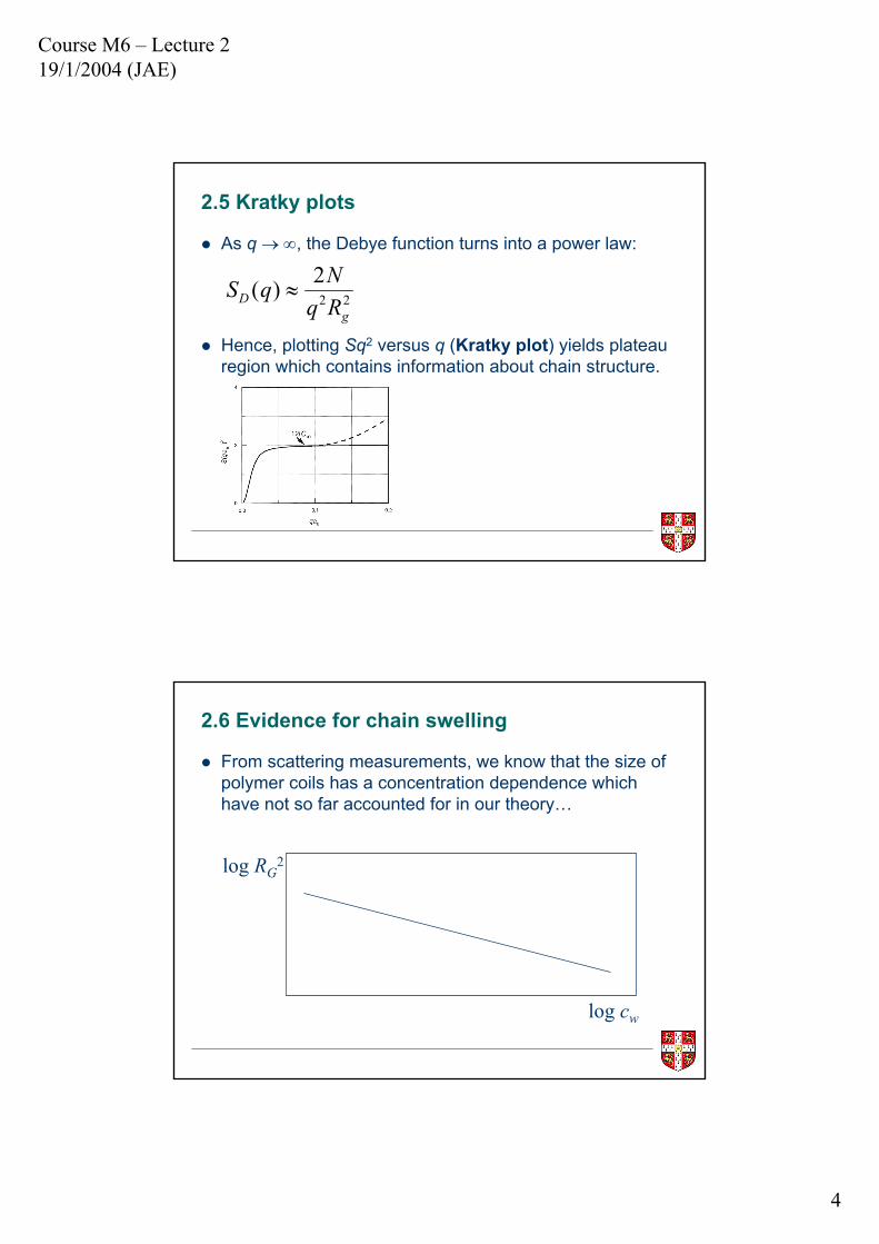
2.5 Kratky plots
As q → ∞, the Debye function turns into a power law:
Hence, plotting Sq2 versus q (Kratky plot) yields plateau region which contains information about chain structure.
222)(
gD Rq
NqS ≈
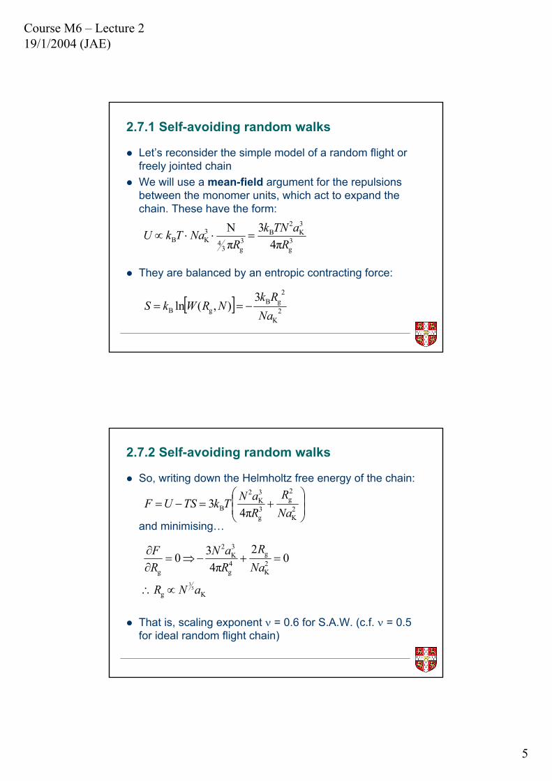
2.6 Evidence for chain swelling
From scattering measurements, we know that the size of polymer coils has a concentration dependence which have not so far accounted for in our theory…
log RG2
log cw
Course M6 – Lecture 219/1/2004 (JAE)
5
2.7.1 Self-avoiding random walks
Let’s reconsider the simple model of a random flight or freely jointed chainWe will use a mean-field argument for the repulsions between the monomer units, which act to expand the chain. These have the form:
They are balanced by an entropic contracting force:
3g
3K
2B
3g3
4
3KB 4π
3πN
RaTNk
RNaTkU =⋅⋅∝
[ ] 2K
2gB
gB
3),(ln
NaRk
NRWkS −==
2.7.2 Self-avoiding random walks
So, writing down the Helmholtz free energy of the chain:
and minimising…
That is, scaling exponent ν = 0.6 for S.A.W. (c.f. ν = 0.5 for ideal random flight chain)
⎟⎟⎠
⎞⎜⎜⎝
⎛+=−= 2
K
2g
3g
3K
2
B 4π3
NaR
RaNTkTSUF
Kg
2K
g4g
3K
2
g
53
02
4π30
aNR
NaR
RaN
RF
∝∴
=+−⇒=∂∂

Course M6 – Lecture 219/1/2004 (JAE)
6
2.7.3 Self-avoiding random walks
The preceding approach is known as the Flory-Fischerargument, and gives almost exactly the same results as exact calculations based on renormalisation group theory (which predict ν = 0.588)
The fact that mean-field theory agree so well with exact calculations is highly surprising!
This is one example of the power of scaling theories in polymer physics (de Gennes)
2.8.1 Polymer melts
What happens now if we consider many polymer chains?Surely the situation will become hopelessly complicated, and the scaling relations will break down? In fact, the situation becomes even more simple…
In a polymer melt, the monomer concentration should be constant, i.e.independent of Rg

Course M6 – Lecture 219/1/2004 (JAE)
7
2.8.2 Polymer melts
This means that there are no net expansive forces, in other words it does not matter whether monomers in contact are part of the same chain or on different chains
Result is that the scaling exponent for an ideal random walk (ν = 0.5) is recovered!!
Statistically speaking, polymer melts are simpler than isolated chains
2.9 Chain collapse
Another simple case is when a polymer experiences a very strong attractive potential
This could be either a low temperatures (we have previously ignored attractive part of vdW force) or when polymer is placed in very poor solvent
This globular state is very important in biopolymers (proteins, DNA) and is also significant in synthetic polymer processing
Simple scaling law i.e. ν = 0.333Kg3
1 aNR ∝

Course M6 – Lecture 219/1/2004 (JAE)
8
2.10 Effect of solvents
Apart from a melt, under what other circumstances can we recover ‘ideal’ scaling?It turns out that, under certain conditions, dilute polymers can also behave as ideal chainsUnder these conditions, the polymer is said to be at its theta point (or Θ-point)At this point, the repulsive forces due to excluded volume are exactly balanced by the compressive forces exerted by the surface tension of the solventIn order to understand why this situation arises, we need a simple model of polymers in solution
2.11.1 Regular solution theory for liquids
Use this to calculate the free energy of mixing in a mean-field approximation on a lattice with effective co-ordination number Z
221211 ε,ε,εinteractions
( )22111221
mix εεε22
−−ΦΦ
=NZU
( )221112B
εεε22
χ −−≡TkZ
21B
mix χ ΦΦ=⇒ NTk
U per site
Course M6 – Lecture 219/1/2004 (JAE)
9
2.11.2 Regular solution theory for liquids
If χ < 0, then there is an enthalpic tendency to mixIf χ > 0, then there is an enthalpic tendency to demixIf χ = 0, the system is termed ideal (athermal)
However, it is the free energy of mixing which determines whether the components actually mixFor simple liquids (not polymers!):
212211B
mix
2211Bmix
χlnln
)lnln(
ΦΦ+ΦΦ+ΦΦ=⇒
ΦΦ+ΦΦ−=
TkF
NkS
per site
Flory-Huggins free energy
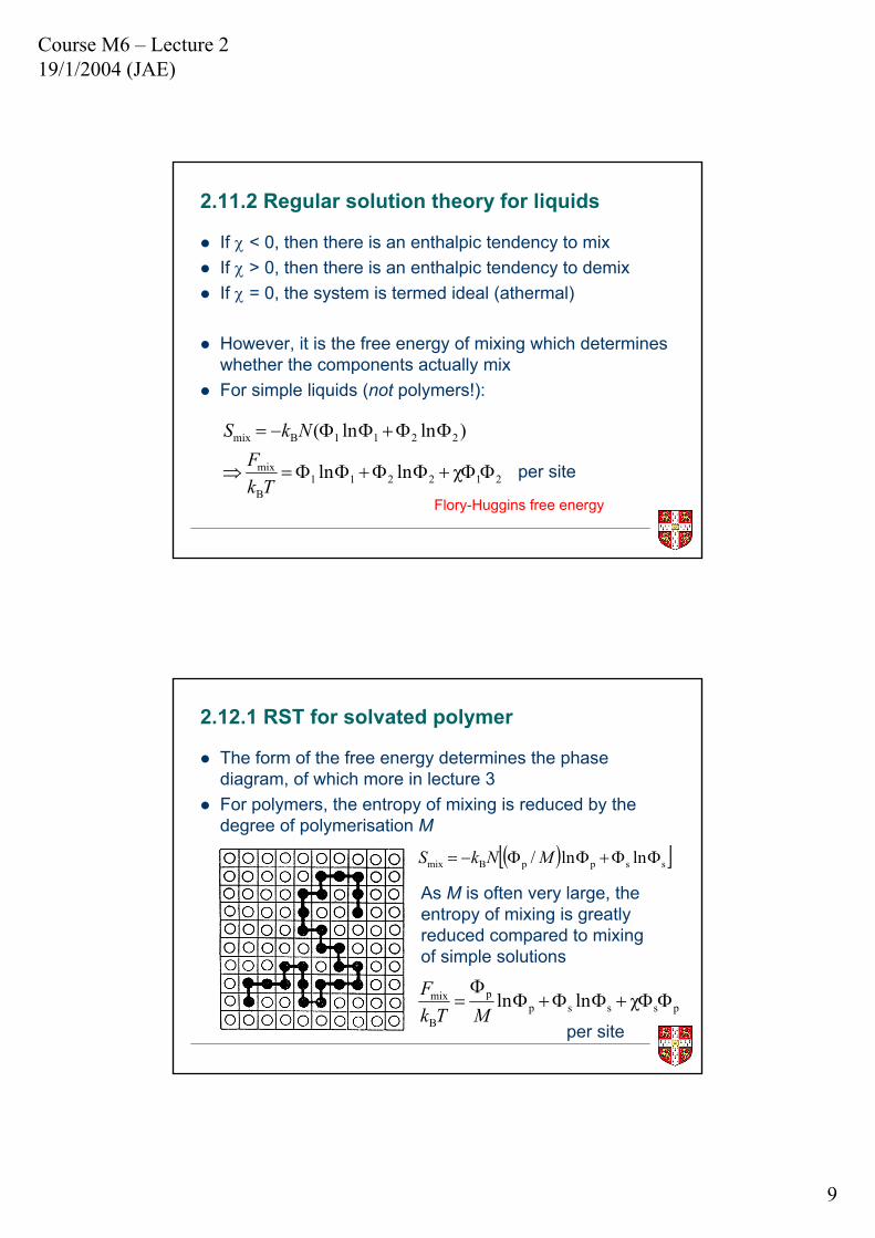
2.12.1 RST for solvated polymer
The form of the free energy determines the phase diagram, of which more in lecture 3For polymers, the entropy of mixing is reduced by the degree of polymerisation M
( )[ ]ssppBmix lnln/ ΦΦ+ΦΦ−= MNkS
As M is often very large, the entropy of mixing is greatly reduced compared to mixing of simple solutions
pssspp
B
mix χlnln ΦΦ+ΦΦ+ΦΦ
=MTk
F
per site
Course M6 – Lecture 219/1/2004 (JAE)
10
2.12.2 RST for solvated polymer
In the context of a binary mixture of polymer and solvent, the χ parameter represents the solvent qualityIf χ < 0.5, then it is said to be a good solventIf χ > 0.5, then it is said to be a poor solventIf χ = 0.5, then it is said to be a Θ-solvent
Vtot
∂∂
−=ΠF
3K
p
aV
npΦ
=3K
mixtot a
VFF =
⎟⎟⎠
⎞⎜⎜⎝
⎛
ΦΦ∂∂
Φ=Φ∂Φ∂
−=Π⇒p
mix
p
2p
p
pmix
)/1()/( FF
2.13.1 Theta conditions
Using the Flory-Huggins form of the free energy, and writing Φp = Φ and Φs = 1 – Φ (binary system), we obtain the following expression for the osmotic pressure:
We can now formulate the Θ-conditions by making power series or virial expansion for osmotic pressure at low Φ
2
B
3K χ
11ln
MΦ−Φ−⎟
⎠⎞
⎜⎝⎛
Φ−+
Φ=
ΠTk
a
( ) 2
B
3K 2
χ21M
Φ−
+Φ
=ΠTk
a Θ-conditions when χ = 0.5
Course M6 – Lecture 219/1/2004 (JAE)
11
2.13.2 Theta conditions
The definition of Θ-conditions is when the second virial coefficient disappears
One of the consequences of this is that χ = 0.5
Since χ is a characteristic of a particular polymer/solvent system, and χ ~ 1/T, then it follows that Θ-conditions will only occur at a certain temperature, the Θ-temperature
This is analogous to the Boyle temperature at which a gas behaves ideally
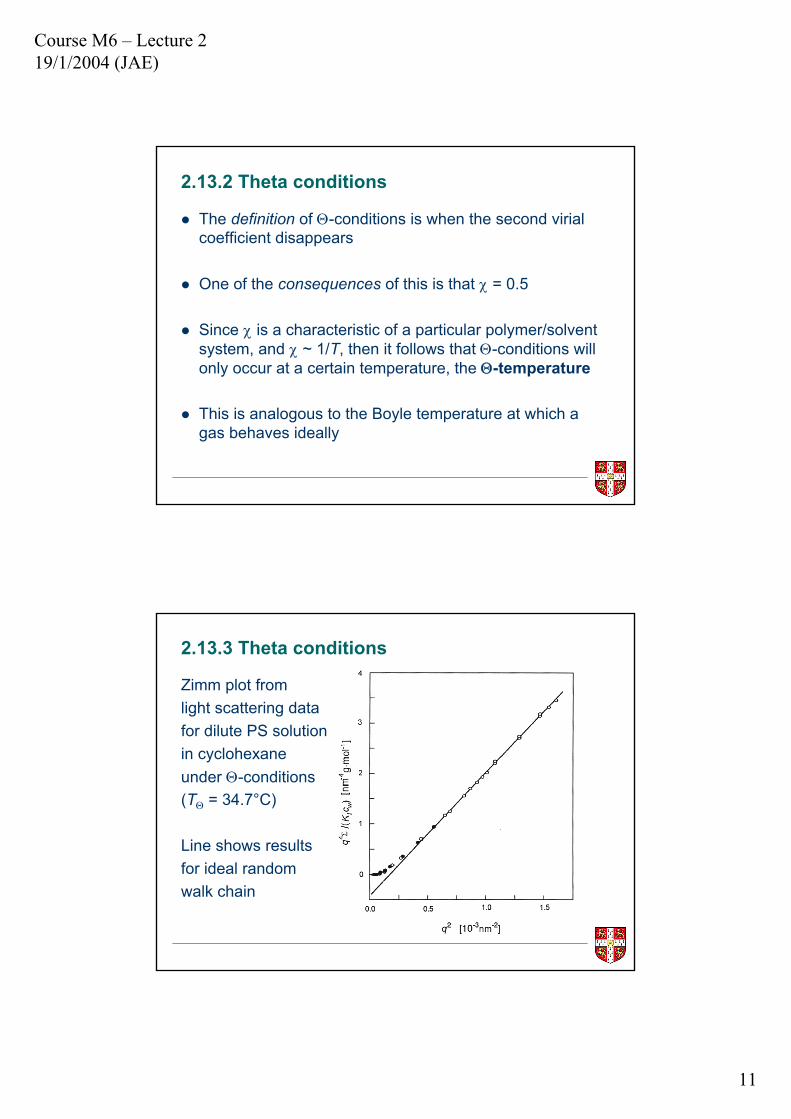
2.13.3 Theta conditions
Zimm plot fromlight scattering datafor dilute PS solutionin cyclohexaneunder Θ-conditions(TΘ = 34.7°C)
Line shows resultsfor ideal randomwalk chain

Course M6 – Lecture 219/1/2004 (JAE)
12
2.13.4 Theta conditions
Concentration dependence of osmotic pressure of PS solutions in cyclohexane around the Θ-temperature
2.14 Good solvents
When χ < 0.5, the polymer is said to be in a good solventThis means that the solvent interacts favourably with the polymer, leading to an expanded chain configuration (with scaling exponent ν > 0.5)Expanded chains behave qualitatively differently to ideal chainsIn particular:
– Asymptotic r → ∞ monomer distribution is negative exponential rather than Gaussian
– Asymptotic r → 0 monomer distribution is zero rather than a maximum
– Rg about 10% smaller than expected from R

Course M6 – Lecture 219/1/2004 (JAE)
13
2.15.1 Scattering data for expanded chains
Chain structure dependent on length scale
Zimm plots from neutron scattering data for dilute solutions of PS in cyclohexane
At temperatures above the theta point (TΘ = 34.7°C) the behaviour at low q becomes non-ideal
2.15.2 Scattering data for expanded chains
At short distances, chains are ideal, whereas at larger distances they behave like expanded chains
Change-over occurs at thermic correlation length

Course M6 – Lecture 219/1/2004 (JAE)
14
Lecture 2 summary
This lecture, we started by introduced some important scattering methods for measuring the dimensions of polymer coils: Zimm, Guinier and Kratky plotsWe then tried to account for the concentration dependence of coil size in dilute solution via the theory of self-avoiding random walksWe found that chains in dilute solution in a good solvent are expanded, but in the melt they are idealChains can also be ideal in solution at their Θ-point, where the attractive enthalpic forces exactly balance the repulsive entropic forcesFinally, we reviewed scaling laws for expanded chains