Pork Barrel Politics and Gerrymandering�

Hideo Konishiy Chen-Yu Panz

September 22, 2015

Abstract

In this paper we propose a tractable model of partisan gerryman-dering followed by electoral competitions in policy positions and trans-fer promises in multiple districts. With such pork-barrel considera-tions, we generally �nd that gerrymandering results in (i) packing theopponent party�s supporters in losing districts, and (ii) more extremepolicies in winning districts. However, depending on the party lead-ers�and voters�preference intensity for policy positions, and depend-ing on how much freedom the leader has in redistricting, we obtaina variety of optimal gerrymandering policies. The well-known pack-and-crack gerrymandering is not necessarily optimal: the party leadermay choose to create some extremely polarized districts to avoid mak-ing costly pork-barrel promises, even with candidates who have morepolarized positions than hers.

Keywords: electoral competition, gerrymandering, policy convergence/divergence,pork-barrel politics

JEL Classi�cation Numbers: C72, D72�Still preliminary. Not for circulations.yHideo Konishi: Department of Economics, Boston College, USA. Email:

hideo.konishi@bc.eduzChen-Yu Pan: School of Economics and Management, Wuhan University, PRC. E-mail

panwhu@126.com

1 Introduction

It is widely agreed that the US Congress has polarized quite a bit in the lasthalf century. The distribution of the House representatives�political positionswere more concentrated at the center of political spectrum with considerableoverlaps between Republican and Democratic representatives�positions in1960s, while it became sharply twin-peaked without overlaps in 2000s (seeFigure 1: by Fiorina, Abrams, and Pope, 2011).1 Simultaneously, Fiorina,Abrams, and Pope (2011) argue that the US voters have not polarized somuch during the same time period. These con�icting observations generatean obvious puzzle: How could the Congress polarize if voters didn�t?[Figure 1 here]One possible explanation is that voters sorted out into Republican and

Democratic parties by their political positions during the period, and thatthe parties�political positions were polarized in party members�preferenceaggregation. Levendusky (2009) suggests that party elites�polarization ledvoter sorting, although it is controversial how much mass polarization ac-tually occurred by voter sorting.2 Recently, Krasa and Polborn (2015) pro-pose a two-party electoral competition model with multiple districts, voterscare not only about the political positions of their local candidates but alsoabout the positions of the parties (which are determined by the elected partyrepresentatives in the legislatures), and show that elected representatives�positions are pulled towards the position of the party�s median voters of thedistricts. Their model can explain the House representatives�polarization atleast partially, as long as the party median voters are pulled away from thecenter by voter sorting.However, more direct explanation for that is partisan gerrymandering in

the US politics. Since the one-person, one-vote decisions by the US SupremeCourt in 1960s, the courts closely examine population equality in districts. Inpractice, however, redistricting is not simply about equaling the populationin each district. It is clear that there is a strong incentive for the party incharge of redistricting to change the political identity of each district to favor

1It is now standard to use a one-dimensional scaling score (DW-Nominate procedureon economic liberal-conservative, Poole and Rosenthal, 1997) to measure representatives�political positions.

2Levendusky (2009) asserts that party elites�polarization clearly caused limited scale ofmass polarization. Fiorina et al. (2011) say that there is little increase in mass polarization,although they admit that party activists�political positions have polarized.

2

the partisan interests.3 Although Ferejohn (1977) �nds little support for ger-rymandering being the cause of declines in competitiveness of congressionaldistricts from mid 1960s to 1980s, Fiorina et al. (2011) state �Many (notall) observers believe that the redistricting that occurred in 2001-2002 had agood bit to do with this more recent decline in competitive seats� the partybehaved conservatively, concentrating on protecting their seats rather thanattempting to capture those of the opposition." (see Fiorina et al. pp. 214-215). They further argue that this decrease in competitiveness is a drivingforce behind the recent political polarization in Congress (see also Gilroux,2001).4

In partisan gerrymandering, two tactics are often discussed. The �rstone is to concentrate or �pack�those who are supporting opponent party inlosing districts. The second is to evenly distribute or �crack�supporters inwinning districts. Introducing uncertainty in each district�s median voter�sposition, Owen and Grofman (1988) consider the situation where a partisangerrymanderer redesigns districts in order to maximize the expected numberof seats or the probability to win a working majority of seats for her party.They assume that the uncertainty in median voter�s political position is localand is independent across districts when the objective is expected numberof seats, and that the uncertainty is global when the goal is the probabilityof winning the majority. Also, they assume that the sum of the positions ofdistrict median voters must stay the same after redistricting (their feasibilityconstraint). They show that the optimal strategy is �packing�the opponentsin losing districts, and �cracking�the rest of voters evenly across the winningdistricts with substantial margins so that the party can win districts even inthe cases of negative shocks under both cases.5 Gul and Pesendorfer (2010)extend Owen and Grofman (1988) by introducing a continuum of districts,and voters�party a¢ liations, and further allow for bipartisan gerrymander-

3One recent example is the 2003 Republican redistricting in Texas that has been con-sidered contributing to Democrat�s defeat in the subsequent election.

4McCarty et al. (2006, 2009) document that the political polarization of the House ofRepresentatives has increased in recent decades, using data on roll call votes. Althoughthey �nd only minor relation between polarization and gerrymandering, Krasa and Polborn(2015) argue that their answer may be incomplete if the political positions of districtcandidates are mutually interdependent.

5The original �cracking�tactics create the maximum number of winning districts withthe smallest margins. In the traditional literature, some argue that gerrymandering willincrease political competition by this reason. In this paper, we use �cracking�tactics inthe sense of Owen and Grofman (1988).

3

ing. They assume that each party leader maximizes the probability of win-ning the majority of seats under more sophisticated feasibility constraints6

by assuming a continuum of districts and generate a �pack-and-crack.�Friedman and Holden (2008), on the other hand, assume that a partisan

gerrymanderer has full freedom in allocating population over a �nite numberof districts, and that she maximize the expected number of seats when thereare only valence uncertainty in median voters� utilities (thus, there is nouncertainty in median voter�s political position). In this idealized situation,they �nd that the optimal strategy is �slice-and-mix�: mixing a slightlylarger number of the most extreme supporters and a slightly smaller numberof the most extreme opponents in the �rst district, then mixing a slightlylarger number of the second most extreme supporters and a slightly smallernumber of opponents in the second district, and so on and so forth. Althoughthis is a very di¤erent prescription for a partisan gerrymanderer, but it is anice benchmark to see what can be done under ideal situation.However, these papers do not model spatial competition in policy posi-

tions, and the elected representatives�positions are implicitly assumed to bethe district median voters�positions (Downsian competition). In contrast,we assume that policy-motivated party leaders compete with their politi-cal positions and pork barrel promises, and we �nd that policy divergenceactually occurs even though our setup is deterministic.7 We analyze the op-timal gerrymandering policies building on this political competition model.With pork-barrel politics, the party leader is aware of the cost of pork-barrelpolicies, and therefore she has strong partisan gerrymandering incentives tocollect their supporters in the winning districts in order to avoid large pork-barrel promises. Our simple model is �exible enough to analyze the optimalpolicies under various feasibility constraints on gerrymandering. It turns outthat we can generate �pack-and-crack�in Owen and Grofman (1988), �slice-and-mix�in Friedman and Holden (2008), and even �pack-and-slice�(see the

6They consider two feasibility constraints. The �rst is the constant mean of medianvoters�positions which is the same as the one in Owen and Grofman (1988). The secondone is that the status quo needs to be a mean-preserved spread of a feasible redistrictingplan.

7In two-party electoral competition model a la Wittman (1983), the equilibrium out-come is the Downsian unless there is uncertainty in median voter�s position (see Roemer2001). In our model, if we place the upperbound on the level of pork-barrel promise, thenthe political competition equilibrium converges to the Downsian as the upperbound goesto zero.

4

following paragraph) as the optimal gerrymandering policies depending onfeasibility constraints, although our model is a deterministic one.The rest of the paper is organized as follows. Section 2 discusses some re-

lated literature. In Section 3, we start with analyzing political-position andpork-barrel competition and characterizing the party leader�s payo¤ fromeach winning district by the district median voter�s position (Proposition1). In Section 4, we investigate the optimal gerrymandering strategy whenthe party leader has complete freedom as in Freedman and Holden (2008),and show that their �slice-and-mix�is also an optimal strategy in our model(Proposition 2). In Section 5, we proceed to the cases where gerryman-derer�s freedom is limited by indivisibility of localities. For tractability ofour analysis, we assume voters�and leaders�cost function in political dis-tance have common constant elasticity > 1. We also assume that eachdistrict has normally distributed voters to justify the feasibility constraintimposed by Owen and Grofman (1988). We show that the optimal gerry-mandering policy may be �pack-and-crack�(Owen and Grofman, 1988), or�pack-and-slice,�in which the gerrymanderer pack the opponent supporters,and slice her supporters from the strongest to moderate in order, dependingon the value of elasticity of cost functions (Propositions 3 and 4). We alsoinvestigate how the results could be a¤ected by an introduction of uncer-tainty in median voters�positions. Unlike in Owen and Grofman (1988), we�nd that �pack-and-slice�becomes more likely than �pack-and-crack�sincein our model, party leaders care about policy positions as well as expectednumber of seats (Proposition 5). Dropping normality of voter distributions,the optimal gerrymandering strategy can be more complicated. Even whenindivisible localities can be ordered in �rst-order stochastic dominance, wecan only show �packing�is optimal, but we cannot generally say much abouthow to allocate supporters over districts as well as the optimal number ofwinning districts. Section 6 concludes. All proofs are collected in AppendixA.

2 Related Literature

Our paper is related to two branches of literature. The �rst one is the pork-barrel literature. In this branch, our model is most related to Lindbeckand Weibull (1987) and Dixit and Londregan (1996). The former introducesa two-party competition model in which (extreme) parties use pork-barrel

5

policies to attract agents with heterogeneous policy preferences. The lattergeneralizes Lindbeck and Weibull (1987) to allow parties having di¤erentabilities in practicing pork-barrel policies, and this di¤erence determines thepork-barrel policy�s target being swing voters or loyal supporters. Our modelis di¤erent from theirs in that we introduce parties�platform decisions be-sides pork-barrel politics, and party leaders choose these two policies simul-taneously.8 Since we try to explain the House representatives�polarization,having platform decisions is essential in our analysis. Moreover, the politicalcompetition result is deterministic in our model which is di¤erent from thesetup with uncertainty in the literature.Second, other than the optimal gerrymandering literature we discussed

in the previous section, there is gerrymandering literature from normativepoint of view as well. This literature focuses on the how the gerrymanderinga¤ects the relation between seats and the vote shares won by a party, so-called �seat-vote curve�. Coate and Knight (2007) identify the social welfareoptimal seat-vote curve and then the conditions under which the optimalcurve can be implemented by a districting plan. With �xed and extremeparties�policy positions, they �nd that the optimal seat-vote is biased towardthe party with larger partisan population. However, Bracco (2013) showsthat, when parties strategically choose their policy position, the directionof seat-vote curve bias should be the opposite. Besley and Preston (2007)construct a model similar to Coate and Knight (2007) and show the relationbetween the bias of seat-vote curve and parties policy choices. They furtherempirically test the theory and the result show that reducing the electoralbias can make parties strategy more moderate.

3 The Model

We consider a two-party (L and R) multi-district model with one party beingentitled to redistrict a state. There are many localities in the state, each ofwhich is considered the minimal unit in redistricting (a locality cannot bedivided into smaller groups in redistricting). We assume that there are L dis-

8Dixit and Londregan (1998) propose a pork-barrel model with strategic ideologicalpolicy decision based on their previous work. However, the ideology policy in their paperis the equality-e¢ ciency concern engendered by parties�pork-barrel strategies. Therefore,the ideology decision in their work is a consequence of pork-barrel politics instead of anindependent policy dimension.

6

crete localities each of which has population 1. The state must haveK equallypopulated districts, and L is a multiple of K. That is, the party in powerneeds to create K districts by combining L

K= n localities in each district.

Locality ` = 1; :::;L has a voter distribution function F` : (�1;1)! [0; 1],where (�1;1) is a space of ideologies in the society and F`(�) is non-decreasing with F`(�1) = 0 and F`(1) = 1. Ideology � < 0 is regarded left,and � > 0 is right. With a slight abuse of notations, we denote the set oflocalities also by L � f1; :::;Lg. A redistricting plan � = fD1; :::; DKg withjDkj = n for all k = 1; :::; K, is a partition of L.9 The gerrymandering party�sleader chooses the optimal district partition � from the set of all possible par-titions �.10 In each district k, the probabilistic distribution function F k isan average of distribution functions of n localities: F k(�) = 1

n

P`2Dk F`(�).

District k�s median voter is denoted by xk 2 (�1;1) with F k(xk) = 12. We

also assume the uniqueness of xk in each districting plan.We model pork-barrel elections in a similar manner with Dixit and Lon-

dregan (1996). A type � voter in district k evaluates party L or R accordingto the utility function with two arguments: one is the policy position of thecandidate representing the corresponding party, � 2 R, and the other is theparty�s pork-barrel transfer t 2 R+. We interpret this pork-barrel transfer asa promise of local public good provision (measured by the amount of mone-tary spending) in the case that the party�s candidate is elected. Formally, avoter � in district k�s utility when party L is the winner is

U�(L) = tkL � c(j� � �kLj) (1)

where �kL is party L�s district k candidate�s policy position, tkL � 0 is party

L�s district-k-speci�c pork-barrel transfer, and c(d) � 0 is the ideology costfunction which is increasing in the distance between a candidate�s positionand her own position. We assume that c(�) is continuously di¤erentiable, andsatis�es c(0) = 0, c0(0) = 0, and c0(d) > 0 and c00(d) > 0 for all d > 0 (strictlyincreasing and strictly convex). Similarly, we have

U�(R) = tkR � c(j� � �kRj)

9A partition � of L is a collection of subsets of L; fD1; :::; DKg, such that [Kk=1Dk = Land Dk \Dk0 = ; for any distinct pair k and k0:10In reality, there are many restrictions on what can be done in a redistricting plan. For

example, a district is required to be connected geographically. Despite the complicationinvolved, our analysis can still be extended to the case with geographic restrictions byintroducing the set of admissible partitions �A � � (see Puppe and Tasnadi, 2009)

7

where �kR is party R�s district k candidate�s policy position and tkR is party

R�s district-k-speci�c transfer.Therefore, voter � votes for party L if and only if

U�(L)� U�(R) = [c(j� � �kRj)� c(j� � �kLj)] + tkL � tkR > 0 (2)

Since the median voter�s type in district k is xk, given �kL, �kR, t

kL and t

kR,

L wins in district k if and only if

Uxk(L)� Uxk(R) = [c(jxk � �kRj)� c(jxk � �kLj)] + tkL � tkR > 0 (3)

Each party leader in the state (of these K districts) cares about (i) thein�uence within her party, (ii) the candidate�s policy position in each dis-trict, and (iii) the district-speci�c pork-barrel spending. We assume that theparty leader prefers to win a district with a candidate�s position closer toher own ideal ideological position and a less pork-barrel promise. The for-mer is regarded as the�policy-motivation�in the literature. By formulatingthe latter, we consider a situation where the leader bears some costs whenimplementing the promised local public goods provision. For example, thebargaining e¤orts needed to push for federal funding. To simplify the analy-sis, we assume that the negative utility by pork-barrel is measured by theamount of money promised. We denote the ideal political positions of theleaders of party L and R by �L and �R, respectively, with �L < �R. Withoutloss of generality, we will set �L = �1 and �R = 1 in the end, but we willstick to notations �L and �R until the gerrymandering analysis starts, whichwould be more helpful to the readers. Formally, by winning in district k,party L�s leader gets utility

V kL = Q� tkL � C(���kL � �L��);

where Q > 0 is the �xed payo¤ (e.g., getting recognition among her partyelites) for winning another district, and C(d) is a party leader�s ideology costfunction with C(0) = 0, C 0(0) = 0, C 0(d) > 0 and C 00(d) > 0 (strictlyincreasing and strictly convex). If she loses in district k, she gets zero utilityfrom the district. Thus, party L�s state leader�s utility from K districts inthe state is

VL =

KXk=1

IL(k)VkL =

KXk=1

IL(k)[Q� tkL � C(���kL � �L��)]; (4)

8

where IL(k) = 1 if L wins, IL(k) = 0 if L loses, and IL(k) = 12if L ties with

R in district k. Similarly, the utility for R is de�ned as

VR =

KXk=1

IR(k)VkR =

KXk=1

IR(k)[Q� tkR � C(���kR � �R��)]: (5)

We introduce a tie-breaking rule in each district based on the relativelevels of the state party leaders�utilities V kL and V

kR . We assume that if two

parties�o¤ers are tied for the median voter xk (Uxk(L) = Uxk(R)) while oneparty�s leader gets a higher (indirect) utility than the other�s, the medianvoter will vote for the party. That is,

Assumption 1. (Tie-Breaking) Given two parties�o¤ers are such thatUxk(L) = Uxk(R), L (R) wins if V kL > V

kR (V

kL < V

kR).

This assumption is justi�ed by the fact that the higher utility is equivalentto the higher ability to provide a better o¤er to the median voter. Especially,consider the case in which two parties are tied and, say, V kL > V

kR = 0, party

L has the ability to provide � > 0 more pork-barrel promise. Therefore, webreak the tie by assuming the median voter prefers L, which is the standardassumptionOur second assumption is a simple su¢ cient condition that assures inte-

rior solutions for both parties.

Assumption 2. (Relatively Strong O¢ ce Motivation) For all feasiblexk, Q � min

�fC(j�j � �j) + c(j� � xkj)g holds for j = L;R.

Notice that if the party leader gets 0 utility, he must o¤er pork-barrelpromise equal to Q � C(j�j � �j). Therefore, the median voter get utilityUxk = Q� C(j�j � �j)� c(j� � xkj). Then, this assumption means that thepayo¤ from winning a district, Q, is large enough so that for any xk, bothparty can o¤er the median voter positive utility, which is a su¢ cient conditionfor the candidate selection problem has interior solution. Also notice thatsince the model only allows a �nite median voters positions, there must exista Q to satisfy this assumption. Moreover, the implication of this assumptionis that it guarantees that in equilibrium both parties promise positive pork-barrel. We will see this more clearly in the next section.11

11This assumption can be weakened signi�cantly. In the Appendix B, we present aweaker condition (Assumption 2�) for interior solutions, and discuss the case of cornersolutions. However, our argument still extend to the cases with corner solutions to someextent.

9

The timing of the game is as follows:12

1. One party, say L, chooses a redistricting plan � = fD1; :::; DKg of L.

2. Given the districting plan in stage 1, party leaders L and R simultane-ously choose local policy positions and pork-barrel promises (�kL; t

kL)Kk=1

and (�kR; tkR)Kk=1, respectively.

3. All voters vote sincerely (with our tie-breaking rule). The winningparty is committed to its policy position and its pork-barrel promise ineach district k = 1; :::; K. All payo¤s are realized.

We will employ weakly undominated subgame perfect Nash equi-librium as the solution concept. We require that in stage 2, party leadersplay weakly undominated strategies so that the losing party leader does notmake cheap promises to the district median voters.13 We will call a weaklyundominated subgame perfect Nash equilibrium simply an equilibrium.

3.1 Electoral Competition with Pork-Barrel Politics

We solve the equilibria of the game by backward induction. We start withstage 2, knowing that voters vote sincerely in stage 3. Notice that the keyplayer is the median voter in the voting stage. Thus, when the leader of partyL makes her policy decisions in district k, she at least needs to match R�so¤er in terms of median voter�s utility in order to win. First, we consider thecase that party L wins (the party R�s leader wins only by providing a strictlybetter o¤er to the median voter). In this case, the leader of party L tries too¤er the same utility to the median voter xk and wins in the district k with

12We can separate stage 2 into two: policy position choices followed by pork-barrelpromises. If we do so, the loser of a district k will get zero payo¤ in every subgame, soit becomes indi¤erent among policy positions. Thus, we need equilibrium re�nement topredict the same allocation. By assuming that the loser party chooses the policy positionthat minimizes the opponent party leader�s payo¤, we can obtain the exactly the sameallocation in SPNE.13The losing party does not su¤er from doing this, since she gets zero utility in losing

districts anyway. The winning party needs to match the o¤er as long as she can get apositive payo¤ by doing so. Demanding players to play weakly undominated strategies,we can eliminate these unreasonable equilibria.

10

the tie-breaking rule. Formally, the party leader�s problem is described by

max�kL;t

kL

fQ� tkL � C(���L � �kL��)g

subject to tkL � c(jxk � �kLj) � �UkR, tkL � 0; and (6)

Q� tkL � C(���L � �kL��) � 0;

where �UkR is the median voter�s utility level from R�s o¤er. Notice thattkL � 0 and Q � tkL � C(

���L � �kL��) � 0 may or may not be binding whiletkL � c(jxk � �kLj) � �UkR must be binding. The solution for this maximizationproblem is straightforward. De�ne �̂(xk; �) by the following equation

c0(jxk � �̂(xk; �)j) = C 0(���� � �̂(xk; �)���): (7)

Notice that (7) is simply the �rst order condition of optimization problem(6) after substituting tkL = c(jxk��kLj)+UkR into the objective function. Theoptimal policy �k

�L = �̂(xk; �L) when �c(jxk � �̂(xk; �L)j) � �UR. That is,

it is not enough for the winning party to win just by only using the policyplatform. Therefore, in this case, it is clear that the optimal pork barrelpromise is

tk�

L = �UkR + c(jxk � �̂(xk; �L)j)Although it seems not clear that tk

�L de�ned above is positive or not, it

turns out that tk�L is always positive, since the similar optimization problem

applies for the losing party and Assumption 2.Now, it is clear that the winning party�s decision is related to what the

losing part proposes in equilibrium. The following lemma shows that thelosing party cannot lose with positive surplus.

Lemma 1. Suppose R is the losing party in district k. In equilibrium,R proposes the policy pair (�k

�R ; t

k�R ) which is the solution of the following

problem

max�kR;t

kR

Uxk(R) = tkR � c(jxk � �kRj)

subject to tkR � 0 and Q� tkR � C(���R � �kR��) � 0

That is, the losing party leader o¤ers a policy position and pork-barrel promisethat leave herself zero surplus in equilibrium.

�k�

R = �̂(xk; �R)

tk�

R = Q� C(����R � �̂(xk; �R)���)11

Moreover, this policy pair is the best she can o¤er for the median voter xk.

The intuition of this lemma is straightforward. If the losing party does noto¤er the median voter the best one, then since the winning party will providethe median voter the same utility level, the losing can always o¤er the medianvoter something better than her original o¤er and win the district. This can-not happen in equilibrium. Therefore, for the losing party R, the equilibriumstrategy is �k

�R = �̂(xk; �R) and tk

�R = Q�C(

���R � �k�R ��). The policy pair pro-vides the median voter with the utility �Uk

�R = Q�C(

���R � �k�R ��)�c(jxk��k�R j).Using this �Uk

�R , one can solve the winning party�s equilibrium pork-barrel

promise tk�L = Q� C(

���R � �k�R ��)� c(jxk � �k�R j) + c(jxk � �k�L j).One thing left to decide is which party should be the winning party.

Notice that, by Lemma 1, the losing party always propose the best o¤er bydepleting all her surplus. Therefore, the party can potentially provide themedian voter with a higher utility level is the winner. Notice that j party�spork-barrel promise is bounded above by j party leader�s payo¤ evaluated at�k�j (otherwise, the leader gets a negative utility):

Q� C(���R � �k�R ��):

Substituting this into median voter�s utility, we obtain

W kR = Q� C(

���R � �k�R ��)� c(jxk � �k�R j);similarly, for party L,

W kL = Q� C(

���L � �k�L ��)� c(jxk � �k�L j);where W k

R and WkL are the (potential) maximum utilities that the median

voter gets from the corresponding party�s o¤er. Therefore, party L wins inthe third stage if and only if

c(jxk � �k�R j) + C(���R � �k�R ��) > c(jxk � �k�L j) + C(���L � �k�L ��); (8)

which simply means that L wins if and only if���L � xk�� < ���R � xk�� : (9)

Proposition 1. Suppose that Assumptions 1 and 2 are satis�ed. De�ne�̂(xk; �) by (7). We have

12

1. For the losing party j, the optimal choice �k�j (x

k; �j) = �̂(xk; �j) which

lies in the interval (xk; �j) (or (�j; xk)).

2. For the winning party i, �k�i = �̂(xk; �i), and tk

�i = Q�C(j�j��k

�j j)�

c(jxk � �k�j j) + c(jxk � �k�i j).

3. Party i wins in the kth district if and only if���i � xk�� < ���j � xk��.

Party�s winning probability Ii(xk) is described by

Ii(xk) =

8<:1 if

���i � xk�� < ���j � xk��12

if���i � xk�� = ���j � xk��

0 if���i � xk�� > ���j � xk�� :

4. The winning payo¤ for the party leader i from district k is

~V ki (xk; �i; �j) = C(�j; xk)� C(�i; xk);

where C(�i; xk) � C(����i � �̂(xk; �i)���) + c(jxk � �̂(xk; �j)j):

5. The winning payo¤ for party i, ~V ki , increases as xk moves away from

�j.

Note that party leaders�policy position choices do not strategically de-pend on the position decisions of the other party. This property of our modelsimpli�es the analysis. Since there is no strategic issue, the winner of thedistrict is determined by which party leader�s position is closer to the medianvoter�s position. Moreover, party leader�s winning payo¤ from the district issimply the di¤erence in the two parties�sums of ideology cost functions ofthe median voter and the party leader.

3.2 Tractable Cost Function

We introduce a convenient special ideology cost function such that bothvoters�and party leaders� cost functions have common constant elasticity.Let C(d) = aCd and c(d) = acd , where > 1, aC > 0, and ac > 0are parameters. In this case both party leaders and voters have the sameelasticity that is constant . In this case, we have the following convenientformula.

13

Claim. Denote A = A(aC ; ac) = aC�

�1+�

� + ac

�1

1+�

� > 0 where � =�

aC

ac

� 1 �1. Suppose that

�QA

� 1 � max

���xk � �L�� ; ��xk � �R�� holds to assureAssumption 2. Normalizing �L = �1 and �R = 1, the winning party leader�sutility from district k, ~V ki (x

k; �i; �j), can be described by

V̂ (��xk��) = � A

����xk��+ 1� � �1� ��xk��� � if��xk�� � 1

A����xk��+ 1� � ���xk��� 1� � if

��xk�� � 1 ;

where (i) V̂ 0 > 0 and (ii) V̂ 00 R 0 , R 2. When = 2, the formulabecomes

V̂ (��xk��) = 4A ��xk��

Since A is a constant, a parameter is the only relevant one to decidethe curvature of payo¤ function. This convenient formula provides a clearinsight in the gerrymandering stage. Also, one can see the importance ofpolitical competition on pork-barrel dimension. Suppose pork-barrel promiseis forbidden in stage 2, one can see that the only equilibrium is Downsianequilibrium. Therefore, the winning payo¤isQ�C(j�i�xkj) which is always aconcave function in xk. However, by considering the pork-barrel promise, theparty has extra spending saving bene�t when xk move closer to extreme whichmakes our payo¤ function di¤erent from the previous one in the literature.

3.3 Gerrymandering Problem

Now, we can formalize the gerrymandering party leader�s optimization prob-lem. Proposition 1 shows that xk = xk(�) is the su¢ cient statistics todetermine the outcome of the kth district. Without loss of generality, as-sume that party L is in charge of redistricting. Notice that the indirectutility of L, ~V kL (x

k; �L; �R), is relevant only when party L wins in district k.The choice of � =

�D1; :::; DK

�a¤ects the party leader L�s payo¤ through�

x1(D1); :::; xK(DK)�via winning chance I(xk(Dk)) in each district k and

its indirect utility ~V kL (xk(Dk); �L; �R): the party L leader�s utility function is

written as

~VL (�; �L; �R) �KXk=1

IL(xk(Dk)) ~V kL (x

k(Dk); �L; �R)

From now on, we suppress �L and �R in indirect utility ~V kL and ~VL. Althoughxk is solely determined by Dk, we can write xk = xk(Dk(�)) = xk(�) for all

14

k = 1; :::; K, since � uniquely determines�D1; :::; DK

�. Thus, we can rewrite

the party leader L�s gerrymandering choice to be the result of the followingmaximization problem

�� 2 argmax�2�

~VL(�)

The SPNE of this game is (��; (�k�L )

Kk=1; (�

k�R )

Kk=1; (t

k�L )

Kk=1; (t

k�R )

Kk=1).

14

4 Gerrymandering with Complete Freedom

As a limit case, let us consider the ideal situation for the gerrymanderer(Friedman and Holden, 2008): there is a large number of in�nitesimal locali-ties with politically homogeneous population: for all position x 2 (�1;1),there are localities `s with F`(x� �) = 0 and F`(x+ �) = 1 for a small � > 0.That is, the gerrymanderer can create any kind of population distributionsfor K districts freely as long as they sum up to the total population distrib-ution. We ask what strategy the gerrymanderer should take. Especially, wewant to ask that whether the gerrymanderer wants to have homogeneous orheterogeneous winning districts in terms of district median locations. First,if the gerrymander loses some districts, she does not care how she loses thosedistricts. Therefore, there are multiple optimal redistricting plans. In orderto pin down the solution, we assume that party L leader tries to make theR party candidates�positions to the left as much as possible whenever shecannot win in some districts. Assume that the optimal number of winningdistricts is K� � K without loss of generality. The question is now how tochoose x1; :::; xK

�to maximize by allocating population to K districts.

In order to highlight the similarity of the result with Friedman and Holden(2008), we will �rst assume F (�1) = 0 and F (1) = 1 (the support of voterdistribution is limited to [�1; 1]), and �L = �1 and �R = 1 so that the partyleaders�political positions the most extreme of all.15

First imagine the situation that the optimal number of winning districtssatis�es K� = 1. By Proposition 1.5, x1 should be as extreme as possible,and then x1 should satisfy F (x1) = 1

2K(x1 is the median voter of the dis-

trict: the most extreme district achievable with population 1K). However,

14The existence of SPNE is guaranteed by the convexity of function c and C and a �nite�.15If we drop the assumption that the party leaders have the most extreme preferences by

Friedman and Holden (2008), the result is modi�ed to involve cardinality of cost functions.See Appendix C.

15

the remaining population to the right of x1 can be anything. For example,if the L�s party leader cares about minimizing R party leader�s payo¤, thenshe will create a district by combining sets

�� � �1L : F (�1L) = 1

2K+ �

K

and�

� � �1R : 1� F (�1R) = 12K� �

K

where � > 0 is arbitrarily small (what is

needed is to make sure that x1 becomes the median voter of the �rst dis-trict). If these two sets compose a district together, then x1 will be de�nedby F (x1) = 1

2K. This is a slice-and-mix strategy for one district to waste

R�s strong supporters�votes. When there are multiple winning districts, thesame logic is applicable. Let �kL 2 [�1; 1] be such that F (�kL) = k

2K+ k�

Kfor

all k = 1; :::; K�, and let �kR 2 [�1; 1] be such that 1� F (�kR) = k2K� k�

K. For

� > 0 small enough, we have

�1 < �1L < ::: < �K�

L < �K�

R < ::: < �1R < 1:

IfK� > 1, the �rst district is composed of all voters with � 2 [�1; �1L][[�1R; 1],district k = 2; :::; K� is composed of all voters with � 2 (�k�1L ; �kL][ [�kR; �k�1R ).That is, let �k be the population measure at district k, then �k((�k�1L ; �kL]) =F (�kL) � F (�k�1L ) = 1

2K= F (�k�1R ) � F (�kR) = �k([�kR; �

k�1R )). All voters

with � 2 [�K�L ; �K

�R ) are packed in losing districts k = K� + 1; :::; K. In this

case, party leader L can pick median voters xk ' �kL approximately for allk = 1; :::; K�. We call this redistricting plan a slice-and-mix strategy,which is proposed in Friedman and Holden (2008). Under the slice-and-mixstrategy, the resulting policy allocations in winning districts is (x1; :::; xK

�) '

(�1L; :::; �K�L ). We will show that this is an optimal policy of choosing winning

district candidates�positions, i.e., gerrymandering. First notice the followingresult.

Lemma 2. Suppose that gerrymanderer can create districts with completefreedom. Suppose that K� < K (there is at least one losing district) andthat x1 � x2 � ::: � xK

�. Also suppose that party L minimizes party R�s

payo¤ in the losing districts (as a re�nement). Then, under the optimalgerrymandering, we have

1. xk < xk+1 for any k and k + 1,

2. �k((xk; 0)) ' 0 holds in all k = 1; :::; K�, i.e., there is no party Lsupporters to the right of the district median xk.

Let Supp(�k) denote the support of �k. Next we can show that, underoptimal gerrymandering, slicing of L supporters occurs.

16

Lemma 3. Suppose that gerrymanderer can create districts with completefreedom. Suppose K� � K with x1 � x2 � ::: � xK�

. Then,�Supp(�k) \ [�1; xk]

�\�

Supp(�k0) \ [�1; xk0 ]

�= ; for all k < k0 � K�.

The two lemmas above show that the above slice-and-mix policy is oneof the optimal policy.

Lemma 4. Suppose that gerrymanderer can create districts with completefreedom, and that �L = �1 and �R = 1. Suppose that K� � K. Then, la-beling districts by the district median voters in ascending order, we havexk = �kL for all k = 1; :::; K� and Supp(�k) \ [�1; xk] = (�k�1L ; �kL] for

k = 1; :::; K�, where �0L = �1. Moreover,K�[k=1

�Supp(�k) \ (xk; 1]

�= [�K

�R ; 1]

holds. Thus, the slice-and-mix strategy is one of the optimal gerrymanderingstrategies, which minimizes party R�s payo¤ in the losing districts, and alloptimal strategies generate the same outcome xk = �kL for all k = 1; :::; K

�

in terms of district median voters.

In Lemma 4, K� is a given number. How does this K� be determined?One can see that, for any k � K�, the position of �kL is independent of themagnitude of K�. Therefore, Lemma 4 implies that the gerrymanderer onlyneeds to win as many districts as possible by using slice-and-mix districtingplan. Let

�K = maxfkj�kL � 0gSince party L�s leader does not care about the losing districts, there

are potentially multiple optimal gerrymandering strategies. The followingproposition characterizes the optimal gerrymandering policy that minimizesparty R�s leader�s payo¤ as a re�nement.

Proposition 2. Suppose that gerrymanderer can create districts with com-plete freedom, and that �L = �1 and �R = 1. The slice-and-mix strategyis one of the optimal gerrymandering strategies, which minimizes party R�spayo¤ in the losing districts. Moreover, K� = �K:

An interesting observation from this proposition is that K� < K meansthat party L is actually the minority party in terms of the state population:the global median xm > 0. Otherwise, party L can win in all districts by usingthe slice-and-mix strategy. However, one party�s monopolizing all districts is

17

rare in US politics partly because of the presence of majority-minority dis-trict requirement (see Shotts (2001)).16 In the case of K� = K, it is obviousthat winning all districts by the slice-and-mix strategy is optimal for gerry-manderer, but the majority-minority requirement forces the gerrymandererseeking for second-best districting plan as a result. It is worthwhile to notethat the slice-and-mix strategy is identical to the optimal policy analyzed inFriedman and Holden (2008). Friedman and Holden (2008) and our papershare the features that (i) the party leader prefers a more extreme medianvoter�s position than a moderate one, (ii) complete freedom in gerryman-dering, and (iii) there is no uncertainty in the median voter�s type unlike inOwen and Grofman (1988) and in the basic model of Gul and Pesendorfer(2010).17 However, there are big di¤erences between our paper and Friedmanand Holden (2008). Our model is based on competitions with political po-sitions as well as transfer promises, while Friedman and Holden (2008) haveneither element in their model. Nonetheless, we can say that the above threecommon conditions are the keys for getting the same results.

5 Gerrymandering with Indivisible Localities

In this section, we will explore how the�slice-and-mix" result would be mod-i�ed if we drop "complete freedom in gerrymandering" (and "no uncertaintyin district median voter�s position" in some cases). We will consider indivisi-ble locality case to accommodate actual geographic elements in redistricting,following the spirits of Owen and Grofman (1988) and Gul and Pesendorfer(2010). In this section, we will largely work on normal distribution case thatjusti�es the paper in Owen and Grofman (1988). Also we use party leadersand voters have cost functions with constraint elasticity denoted by , al-though we did not need to assume any additional condition on cost functionsof party leaders and voters in the complete freedom case.Let the party leaders� and voters� cost functions be C(d) = aCd and

c(d) = acd , where > 1, aC > 0, and ac > 0, and let us normalize �L and �R16In fact, even though either one of the two parties must be the majority in a state,

the majority party usually does not win all districts. This can be attributed to Section2 of the Voting Act Rights (accompanied with other United States Supreme Court cases)which essentially avoid the minority votes being diluted in the voting process similar toour slice-and-mix strategy.17Gul and Pesendorfer (2010) also include aggregate uncertainty, generalizing Owen and

Grofman (1988).

18

at �1 and 1, respectively. As we have seen before from Claim (the propertiesof constant elasticity cost functions), if

�QA

� 1 � max

���xk � �L�� ; ��xk � �R��(a su¢ cient condition for interior solutions), the winning party i�s leader�sutility from district k is

~V ki (xk) = V̂ (

��xk��) = C(�j; xk)� C(�i; xk) = A ����xk��+ 1� � �1� ��xk��� �where A is a constant. As is shown in Claim, we have (i) V̂ 0 > 0, and (ii)V̂ 00 R 0 if and only if R 2. This result (ii) may require some explanation.The readers may be puzzled by having concave V̂ function under 1 < < 2,since cost functions C(�j; xk) and C(�i; xk) are always strictly convex in

��xk��.The reason for (ii) to happen is that V̂ subtracts a strictly convex functionfrom another strictly convex function, and such a function can be anything ingeneral. If the cost function is a constant elasticity type, however, we happento be able to say that V̂ is strictly concave or strictly convex depending on R 2.Now, consider two partitions � and �0 such that Dk0(�) = Dk0(�0) for all

k0 6= fk; ~kg. Thus, Dk(�0) andD~k(�0) are created by swapping some localitiesbetweenDk(�) andD~k(�): i.e., S = Dk(�)nDk(�0) = D

~k(�0)nD~k(�) and T =D~k(�)nD~k(�0) = Dk(�0)nDk(�) are swapped. Is such swapping bene�cial to

the gerrymandering party leader? By swapping localities S and T , xk and x~k

must move in the opposite directions. We call a swap �cracking�if the medianvoters of two districts involved moves closer to each other after swapping anda swap �anti-cracking�if the opposite happens.We will consider the case in which voters�distribution in each locality

follows a normal distribution.

5.1 Normally Distributed Voters

Owen and Grofman (1988) analyzed the optimal partisan gerrymanderingpolicy by imposing a constraint such that the sum of xks,

PKk=1 x

k(�), muststay constant for all �. They obtained the famous pack-and-crack result whenthe party leader maximizes the number of seats under this constraint. In ourindivisible locality case, if each locality has normally distributed voters, thefeasibility constraint becomes exactly this constraint (the proof is obvious bynoting that the median is equivalent to the mean under normality).

19

Lemma 5. Suppose that the voter distribution in each locality is normaldistributed, i.e., F` � N(�`; �`) for each ` 2L. Then, the median of districtk is

xk(�) =1

n

X`2Dk(�)

�`:

This lemma automatically implies thatPK

k=1 xk(�) must stay constant,

sincePK

k=1 xk(�) = 1

nK

P`2L �`: Therefore, under the normal distribution

assumption, swapping the sets of localities S and T between districts k and~k, we have

� = xk(�0)� xk(�) =P

`2T �` �P

`2S �`

n= x

~k(�)� x~k(�0);

while xk(�0) + x~k(�0) = xk(�) + x~k(�). Without loss of generality, assume

x~k(�0) < x

~k(�) < xk(�) < xk(�0) < 0. This means that � is more crackedthan �0, and we have

~VL(�0)� ~VL(�)

=�~V kL (x

k(�0)) + ~V~kL (x

~k(�0))���~V kL (x

k(�)) + ~V~kL (x

~k(�))�

=�V̂ (��xk(�0)��) + V̂ ����x~k(�0)������ �V̂ (��xk(�)��) + V̂ ����x~k(�)�����

Since function (�) �1 is strictly concave or strictly convex depending on < 2 or > 2, respectively. As is easily seen from Claim and Figure 1,if < 2 ( > 2) then cracking from �0 to � improves (reduces) party L�sleader�s utility, but if = 2 then there is no e¤ect. Thus, depending onthe value of ,�cracking" can be a good or bad strategy.18 When > 2holds, concentrating supporting voters from the strongest to moderate ones,or �slicing�is optimal.

Proposition 3. Suppose that party leaders and voters have constant elastic-ity cost functions, and that the voter distribution is normal in each locality.

18Puppe and Tasnadi (2009) consider a model in which party cares about only thenumber of seats and geographical constraints on feasible districting plan. They show thatpack-and-crack does not generally work.

20

Then, cracking is preferable when < 2, while slicing is preferable when > 2. When = 2, cracking or slicing does not matter. 19

[Figure 2 here]

The reason that the result varies depending on the value of is that theparty leader has policy preference.20 When > 2, V̂ (

��xk��) = A[���xk��+ 1� ��1�

��xk��� ] is strictly convex in ��xk��, which means that slicing is bene�cial.This is because the opponent party leader�s cost of matching xk�s utility isincreasingly high which implies that the winning party�s leader can save a lotof money in such a district. We can show that the optimal gerrymanderingpolicy depends on R 2, and we obtain the famous pack-and-crack resultwhen < 2. In contrast, when > 2, then pack-and-slice is the optimal.In order to characterize the optimal gerrymandering policy for > 2

under our normality assumption, it is useful to order localities by their means.Let ` < `0 mean �` � �0`. Then, since xk = �k = 1

n

P`2Dk �` hold, if

party L cannot win all districts, it is bene�cial to pack party R supportinglocalities. Let �xk = 1

n

Pnk`=n(k�1)+1 �` < 0 for all k = 1; 2; :::; K, and let

�K � K be a nonnegative integer such that �x �K < 0 and �x �K+1 � 0. Let us callthe allocation (�xk) �Kk=1 a pack-and-slice gerrymandering policy. This policypack all opponents in unwinable districts, and slices supporting voters fromthe most extreme to moderate in order. This involves districts with votergroup who are even more extreme than the party leader. This is becausewith convex V̂ , the opponent party�s cost to attract the median voter ofsuch a district is so high, and the winning party�s leader does not need topay much in the pork-barrel politics. Thus, if > 2, we have the followingcharacterization of the optimal gerrymandering policy.

Proposition 4. Suppose that party leaders and voters have constant elas-19Given this observation, some information about optimal gerrymandering strategy can

be derived. Suppose that the gerrymandering party L wins K� districts and > 2. Werank the winning district such that x1 < x2 < ::: < xK

�. Also, we rank the localities

in winning districts by `1 < `2 < ::: < `nK�. Then it is optimal for the gerrymanderer

to pack n most extreme localities into district 1 and n next most extreme localities intodistrict 2 and so on. It is obvious that any other districting plan is not optimal since therealways exists a anti-cracking swap.20The shape of payo¤ function depends on the ideology and pork barrel cost functions.

There is no reason to believe those cost functions following some particular forms. On theother hand, in Gul and Pesendorfer (2010) the shape of payo¤ functions depends on theshape of local shock distribution. It is more reasonable to assume concavity in their setup,justifying �pack-and-crack.�

21

ticity cost functions with > 2, and that the voter distribution is normalin each locality. Then, the optimal gerrymandering policy is described bypack-and-slice with (�xk) �Kk=1.

How about the case with < 2? By the same logic above, it is easyto see that the optimal policy must be to �pack-and-crack�, but it is hardto characterize the policy by the following two reasons: (i) there are manylocally optimal cracking district plans but it is hard to say which one is thevery best due to the integer problem, and (ii) the optimal number of winningdistricts is hard to characterize. For the second point, see the followingexample.

Example 1. Suppose < 2. There are 20 SL-type localities in which thevoter distribution is normal and the mean voter is�1 (Strong Left supporter),5 WR-type localities with mean voter 0:1 (Weak Right supporter), and 5SR�type localities with mean voter 1 (Strong Right supporter). Each districtmust include 5 localities and there are 6 districts. If the gerrymandering partyis L, the optimal districting plan must group the SR�type localities together.The gerrymanderer must decide between grouping 4WR localities with 1 SLin �ve winning districts or grouping 5 SL localities in four winning districts.Then the decision is to win 4 districts with xk = 1 or to win 5 districts withxk = 0:78. The payo¤ di¤erence between these two plan is

D = A[4� 2 � 5� ((1:78) � (:22) )]

When < 1:226 and > 1:619, D > 0 which means that L should formstrongly winning district and lose a relative moderate district. Otherwise,D < 0 means that the party should win more districts by forming weakerwinning districts. This example shows that the decision of the number ofwinning districts is not monotonic and trivial even in the case under thenormal distribution assumption.

5.2 With Uncertainty

In this subsection, we extend our discrete locality setup to include uncer-tainty. This extension can make an interesting comparison with the resultin the gerrymandering literature. Up to this point, our model is a deter-ministic model. This is to say that when the gerrymandering is done, both

22

parties can predict the outcome of elections with perfect accuracy. How-ever, this might oversimpli�es the real world gerrymandering problem. Inthe U.S., since the redistricting is decennial, there is usually a time gap be-tween redistricting and election. Even though the gerrymanderer may havea great amount of freedom and information when redistricting is conducted,the positions of district median voters can still be modi�ed by demographicchanges that take place after gerrymandering is conducted. In other words,the gerrymander faces some uncertainty in the positions of district medianvoters. A common approach of modeling uncertainty is to assume local un-certainty that the positions of district median voters are a¤ected by i.i.d.district-speci�c shocks. These shocks realize after redistricting. How doesthe gerrymandering strategy change in the presence of uncertainty? An in-tuitive argument is that, since now a winning district can become a losingone when the shock hits, the gerrymanderer would prefer to win by a largermargin. Therefore, the presence of uncertainty seems to enhance the incen-tive to cracking the supportive localities to avoid winning with small marginin a mild (ex ante) supporting district. This intuition is the fundamentalreason behind Owen and Grofman (1988). Does the same argument applyto our case with policy-motivated gerrymanderer?Let local shock yk be a random variable with density function gk :

[�1;1] ! R+ and yk being a representative realization. We also assumethat yk�s are i.i.d. and denote gk = g. We also normalize the mean so thatE(yk) = 0. After yk realizes, the k district�s median voter position shiftsfrom xk(�) to xk(�) + yk. We also modify the timing of the game as thefollowing:

1. One party, say L, chooses a districting partition � = fD1; :::; DKg ofL.

2. Nature plays and the local shock yks are realized.

3. Party leaders L and R simultaneously choose policy positions and pork-barrel promises (�kL; t

kL)Kk=1 and (�

kR; t

kR)Kk=1 (under the above behavioral

assumption), respectively.

4. All voters vote sincerely (with our tie-breaking rule). The winningparty is committed to its policy position and its pork-barrel promise ineach district k = 1; :::; K. All payo¤s are realized.

23

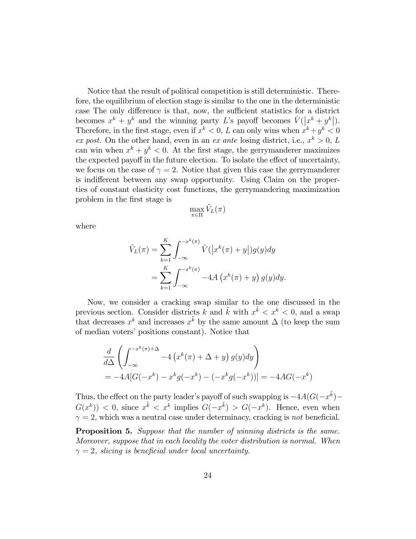
Notice that the result of political competition is still deterministic. There-fore, the equilibrium of election stage is similar to the one in the deterministiccase The only di¤erence is that, now, the su¢ cient statistics for a districtbecomes xk + yk and the winning party L�s payo¤ becomes V̂ (

��xk + yk��).Therefore, in the �rst stage, even if xk < 0, L can only wins when xk+yk < 0ex post. On the other hand, even in an ex ante losing district, i.e., xk > 0, Lcan win when xk + yk < 0. At the �rst stage, the gerrymanderer maximizesthe expected payo¤ in the future election. To isolate the e¤ect of uncertainty,we focus on the case of = 2. Notice that given this case the gerrymandereris indi¤erent between any swap opportunity. Using Claim on the proper-ties of constant elasticity cost functions, the gerrymandering maximizationproblem in the �rst stage is

max�2�

~VL(�)

where

~VL(�) =KXk=1

Z �xk(�)

�1V̂ (��xk(�) + y��)g(y)dy

=KXk=1

Z �xk(�)

�1�4A

�xk(�) + y

�g(y)dy:

Now, we consider a cracking swap similar to the one discussed in theprevious section. Consider districts k and ~k with x~k < xk < 0, and a swapthat decreases xk and increases x~k by the same amount � (to keep the sumof median voters�positions constant). Notice that

d

d�

Z �xk(�)+�

�1�4�xk(�) + � + y

�g(y)dy

!= �4A[G(�xk)� xkg(�xk)� (�xkg(�xk))] = �4AG(�xk)

Thus, the e¤ect on the party leader�s payo¤of such swapping is�4A(G(�x~k)�G(xk)) < 0, since x~k < xk implies G(�x~k) > G(�xk). Hence, even when = 2, which was a neutral case under determinacy, cracking is not bene�cial.

Proposition 5. Suppose that the number of winning districts is the same.Moreover, suppose that in each locality the voter distribution is normal. When = 2, slicing is bene�cial under local uncertainty.

24

Corollary. In the same setup as Proposition 5, introduce of local uncertaintymake the �pack-and-slice�strategy optimal even then = 2.

Strikingly, our result is the opposite of pack-and-crack strategy in Owenand Grofman (1988). The reason behind it is that in Owen and Grofman(1988), the party only cares about winning probability and do not care aboutthe cost of winning a district. The only reason a gerrymanderer move theposition of a median voter is that this operation yields a higher winningprobability. In Owen and Grofman (1988), the party leader�s objective is thesum of winning probabilities (i.i.d.):

max�2�

WL(�; �L; �R)

where

WL(�; �L; �R) =KXk=1

Z �xk(�)

�1g(y)dy

Let us do the same exercise of a cracking swap between districts k and ~k(decreasing xk and increasing x~k by the same amount � > 0). Furthermore,we assume that the distribution g is unimodal. Then, the e¤ect on the partyleader�s payo¤ of such swapping is �(g(�x~k)� g(xk)) > 0, since x~k < xk < 0implies g(�x~k) < g(�xk) by unimodality. Hence, cracking is bene�cial ifthe party leader does not care about policy positions. However, in our case,the gerrymanderer cares about the winning probability and the position ofmedian voter. An extreme median voter not only gives a higher winningprobability but also a low pork barrel cost. This extra incentive makes anextreme redistricting plan more attractive under = 2. This means thateven if < 2, there can be cases that anti-cracking is bene�cial to the partyleaders, despite that the payo¤ function is concave in xk.

5.3 Without Normality: The Case of FOSD-orderedLocalities

What if we drop the linearity embedded in the normal distribution assump-tion? Once normality is dropped, we can no longer use the result of Lemma5: if some localities are swapped between districts k and ~k, then the sizes ofthe shifts of xk and x~k are unknown though the directions of the moves areopposite. This makes the analysis very complicated, so we will consider the

25

case where localities are ordered in the �rst-order stochastic domina-tion (FOSD) in their voter distributions over the political spectrum, andthe gerrymanderer can create political districts by using any combination oflocalities. Formally, we assume the following:

Assumption 3. (FOSD) The set of localities L is FOSD-ordered if forevery pair of localities `; `0 with ` < `0, we have (i) F`(�) > F`0(�) for all� 2 [�1; 1], or (ii) F`(�) = F`0(�) for all � 2 [�1; 1]. Any combination of nlocalities can form a political district.

That is, smaller number localities are more leaning towards L party, andas the number increases localities are leaning more towards R party. Thefollowing property is the direct consequence of FOSD-ordered localities.

Lemma 6. Suppose that L is FOSD-ordered. Let ` 2 Dk and `0 =2 Dk

be such that `0 < ` and F` 6= F`0, and let Dk0 = (Dk [ f`0g)nf`g. Then,xk(Dk0) < xk(Dk) holds.

This result is a direct consequence of the FOSD-ordered localities.21 Thequali�cation F` 6= F`0 implies case (i) of the FOSD de�nition holds, and thedistrict median moves to left by replacing locality ` by locality `0. RecallProposition 1.5 that ~V kL (x

k; �L; �R) = C(�R; xk) � C(�L; xk) is a decreasingfunction in xk, we have the following result:

Proposition 6 (Weak Segregation). Suppose that L is FOSD-ordered.For simplicity, suppose further that �L = �1 and �R = 1. Then, under theoptimal gerrymandering, there is a locality `� such that all localities ` with` � `� belong to L�s winning districts, while all localities ` with ` > `� belongto losing districts, unless there are completely tied districts.

This result is reminiscent to the packing gerrymandering strategy men-tioned above. Thus, if localities are not �ne enough to allow us slice-and-mixstrategies, and localities are FOSD-ordered, the gerrymanderer packs thoserelatively unfavorable localities to form losing districts in ��. Again note thatthis packing result is obtained under deterministic model unlike Owen andGrofman (1988). Our result is based on the assumption of the FOSD-ordered

21Suppose that FOSD assumption does not hold, even if ` has a larger median than `0

does, it is possible that xk(Dk0) � xk(Dk) where Dk0 = (Dk [ f`0g)nf`g. One can replaceFOSD assumption by simply assuming that the median voter increases when replace alocality with any other one with higher median.

26

localities and the slope of winning payo¤ function. The FOSD assumptionmay sound strong, but there are geographical constraints in redistricting inthe real world. If this were the case, the principle of the proof of the propo-sition might still work even if localities are not exactly ordered according toFOSD.Now we turn to the other side of the traditional strategy in Owen and

Grofman (1988), cracking one�s supports to form homogeneous winning dis-tricts. We consider a similar swapping localities between two districts k and~k as before. However, with FOSD assumption, we cannot say much abouthow this swap will a¤ect xk and x~k except for the opposite directions of mov-ing (, say, decreasing xk and increasing x~k). Generally speaking, the crackingstrategy creates more homogeneous districts. It increases ~V ~kL but decreases~V kL . The characterization of these two e¤ects depends on the shape of costfunctions (c and C, as we have demonstrated in the normality case) and allF`�s. Therefore, it is di¢ cult to derive the optimal gerrymandering strategyin general. To compare with the previous argument, we again consider thecase of common elasticity cost functions with = 2 but consider generallocality distributions.

Example 2. Suppose that �L = �1 and �R = 1. We now consider asimple case with 6 localities L = fl; l; wl; wl; r; rg where locality l stands forleft-leaned locality with the distribution Fl and the median position xl lessthan 0. A locality r is right-leaned with the median lager than 0. A localitywl is the weakly left-leaned with the median position equal to �xwl 2 (xl; 0).Also we assume that aC = ac = 1, = 2, and Q > 1.

In this case, there are two possible optimal districting plan for L: D =ffl; wlg; fl; wlg; fr; rgg or D0 = ffl; lg; fwl; wlg; fr; rgg. We can easily com-pare these two districting plans. Notice that these two plans both packing theunfavorable localities to form the losing district in accordance with Propo-sition 6. The former one cracking the strong supportive localities (fl; lg inthis example) into the winning districts, i.e., pack-and-crack. In contrast,the second plan slices supportive localities in the winning district, i.e., pack-and-slice.

Proposition 7. In Example 2 with = 2, fl; l; wl; wl; r; rg and K = 3,L (strictly) prefers cracking, i.e.,districting plan D over D

0, if and only if

12(xl+xwl) = 1

2(xfl;lg+xfwl;wlg) > xfl;wlg, which is equivalent to

R 12(xl+xwl)

xlfld� >R xwl

12(xl+xwl)

fsd�.

27

There is no reason to believe the last inequality to hold or not, since it isnot related to the FOSD assumption. This inequality means that L prefersD if voters in his strong supporting localities are more clustered around the

median than those in the weak supporting localities.22 IfR 1

2(xl+xwl)

xlfld� >R xwl

12(xl+xwl)

fsd� holds and L crack strong supporters with weak ones in thewinning district, the median voter will be pulled toward left a lot due tothe fact that the strong supporting locality is more clustered. In this case,L wins both districts and the costs of pork-barrel transfer is moderate. Onthe other hand, if the inequality fails to hold, weak winning district woulddemand too much money and the equilibrium policy would be too far awayfrom �L. Therefore, instead of pack-and-crack, the gerrymanderer shouldchoose pack-and-slice. Note that = 2 is a special case that makes ~V kL linearin xk. Compare with the normality case, this example isolates the e¤ect oflocality distribution from the curvature e¤ect shown in the normality case.If > 2 or 1 < < 2, then although each agent�s cost function is convex,function ~V kL becomes strictly convex and strictly concave in x

k, respectively.Under such situations, it becomes even harder to say if cracking is the rightstrategy.

6 Conclusion

In this paper, we propose a gerrymandering model with endogenous candi-dates�political positions, in which two parties compete in their positions andpork-barrel politics. Even though we mostly assume deterministic outcomes,we can generate policy divergence unlike Wittman (1983). We derive the op-timal partisan gerrymandering policies under di¤erent circumstances� fromthe case of the gerrymanderer having full freedom in redistricting to the caseswith indivisible localities with various voter distributions.Our model is �exible enough to analyze the optimal policies under vari-

ous feasibility constraints in gerrymandering. The results depend on circum-stances. We obtain �slice-and-mix,��pack-and-crack,�and �pack-and-slice�strategies, some of which are obtained in di¤erent gerrymandering models in

22To be more precise, the inequality requires that voters who is relatively right (com-pared to the median, i.e., � 2 [xl; 12 (x

l + xwl)]) in l have a larger population mass thanvoters who relatively left (� 2 [ 12 (x

l + xwl); xwl]) in wl.

28

the literature.There are possibly interesting extensions. The �rst one is to introduce

the uncertainty into our model. Our conjecture is that, if the uncertainty isin�nitesimal, e.g., the gerrymander can only observe that the median voter�sposition belongs to the interval [xk��; xk+�] for � being a (small) preferenceperturbation and if the gerrymanderer has complete freedom in redistricting,the slice-and-mix strategy may still be optimal à la Friedman and Holden(2008). However, with signi�cant uncertainty in median voters�positions likein Gul and Pesendorfer (2010), we do not know what can happen. Second,in this paper we concentrated on one type of pork-barrel politics: candidates�promise� transfer contingent to their winning the districts. This kind ofpromises are di¤erent from campaign �nancing. In the latter case, even if acandidate loses in a district, the spent campaign expenditure will not comeback. In some circumstance, such a model may be more realistic. Theseextensions are subject to future research.

Appendix A: Proofs

Proof of Lemma 1. First, by Assumption 2, the non-negativity constraintof tkR is not needed. There are three cases: if R loses with Q � tk

�R �

C(���R � �k�R ��) > 0 and its o¤er gives the median voter utility equal to �U

in equilibrium, it must be that L wins with positive indirect utility and alsoprovides the median voter with the utility level �U . However, this meansthat R can win the election by providing, say, � more pork-barrel promise.This contradicts with the equilibrium condition. The second case is thatQ� tk�R �C(

���R � �k�R ��) = 0 but Uxk(R) is not maximized. In this case, theremust exist some points (t0�0) which satis�es Q � t0 � C(j�R � �0j) = 0 butthe pair provides the median voter strictly higher utility. Then any pointon the segment connecting (t0; �0) and (tk

�R ; �

k�R ) is strictly better o¤ for both

R and the median voter xk by the strict convexity of the preferences. Acontradiction. The third case, Q� tk�R � C(

���R � �k�R ��) < 0, cannot happen,since the strategy that generates a negative payo¤ is a dominated strategyfor R�s leader. �Proof of Proposition 1 The proofs of part 1 to 3 are in the main text. ~V kican be derive from substituting the equilibrium tk

�i into the utility function

of winning party i. As for part 5, we �rst set i = L and take derivative of~V kL with respect to x

k. There are two cases: if �L � xk, d~V kLdxk

= �c0k�R � xk)�

29

c0k � �k�L ) < 0: If �L > xk,d ~V kLdxk

= �c0k�R � xk) + c0k�L � xk) < 0: The inequalitystill holds since c(�) is an increasing function and �k�L � xk < �k�R � xk.�Proof of Claim. By Proposition 1, if �L < xk then �kL 2 (�L; xk) is charac-terized by aC

��kL � �L

� �1= C 0

��kL � �L

�= c0

�xk � �kL

�= ac

�xk � �kL

� �1,

or � =�aC

ac

� 1 �1

=xk��kL�kL��L

. Thus, �k�L = �L+�xk

1+�, and

C��k�L � �L

�+ c�xk � �k�L

�= aC

��

1 + �

�xk � �L

�� + ac

�1

1 + �

�xk � �L

�� =

�aC�

�

1 + �

� + ac

�1

1 + �

� ��xk � �L

� = A

�xk � �L

� ; (10)

where A = A(aC ; ac) = aC�

�1+�

� +ac

�1

1+�

� > 0. Thus, in general, the sum

of the party leader�s and the median voter�s costs C(�i; xk) can be written as

C(�i; xk) = A���xk � �i��� :

If A(aC ; ac)���xk � �i��� � Q for both parties i = L;R, then Assumption 2

is satis�ed. Then, Proposition 1.4 implies that if party i is the winner indistrict k (i.e.,

��xk � �i�� < ��xk � �j��), then party i�s winning payo¤ is~V ki (x

k; �i; �j) = A����xk � �j��� � ���xk � �i��� �

Let �L = �1 and �R = 1 without loss of generality.�Proof of Lemma 2. First, we show that xk < xk+1 by contradiction. Ifxk = xk+1, then by swapping � measure population of the right-most voterin [�1; xk] in district k with � measure population of the left-most voter in[�1; xk+1] in district k+1, party L can move xk to the left without changingxk+1 which strictly increases L leader�s payo¤ by Proposition 1.5. Thus, wehave xk < xk+1. For the second part, suppose that �k((xk; xk+1)) > 0. In thiscase, by swapping them with the same measure of people within (xk; xk+1)in district k to the right of xk+1, she can move xk+1 to the left. This isa contradiction. Thus, the optimality requires �k((xk; xk+1)) = 0. Then,suppose that �k((xk+1; 0)) > 0 holds. In this case, party L leader can movelosing districts�candidate to the left by swapping the district k populationin the interval (xk+1; 0) with the party R supporters in losing districts. This

30

is again a contradiction. For the case k = K�, if �k((xk; 0)) > 0 holds, thenby swapping this population with the losing districts�right-wing population,the losing districts�candidates can be moved to the left which is not optimal.Hence, �k((xk; 0)) = 0 must hold for all k = 1; :::; K�.�Proof of Lemma 3. The proof is rather obvious. From Lemma 2, weknow that x1 < x2 < ::: < xK

�holds, and that �k((xk; 0)) = 0 for all

k = 1; :::; K�. Thus, if�Supp(�k) \ [�1; xk]

�\�Supp(�k

0) \ [�1; xk0 ]

�6= ;,

then by swapping the population at the most left in district k0 and thosevoters at the most right within [�1; xk] in the district k, party L leader canmove xk to the left without xk

0intact. This is a contradiction.�

Proof of Proposition 4. When > 2, V̂ (��xk��) = A[���xk��+ 1� ��1� ��xk��� ]

is convex in��xk�� even for the case of ��xk�� � 1. This convexity makes slicing

policy is more preferable than cracking within the winning districts, result-ing in �K winning districts. Noting the gerrymandering party leader getszero payo¤ from the losing districts, the party does not want to increase thenumber of winning districts by moving supporting voters to another district.Given the convexity of V̂ , it does not pay to dilute their supporters.�

Proof of Proposition 6. Recall that party Lmaximizes ~VL(�) =KPk=1

IL(xk(Dk)) ~V kL (x

k(Dk)).

Thus, what is relevant is to maximize the indirect utilities of party L�sleader from her winning districts. Suppose that there is a pair ` 2 Dk

and `0 2 Dk0 under ��, where I(xk(Dk)) = 1 and I(xk0(Dk0)) = 0, re-

spectively. Then, by swapping ` and `0, I(xk((Dk [ f`0g)nf`g)) = 1 andI(xk

0((Dk0 [ f`g)nf`0g)) = 0 still hold, while xk((Dk [ f`0g)nf`g) < xk(Dk)

and xk0((Dk0 [ f`g)nf`0g) > xk0(Dk0) must follow by Lemma 6. By Proposi-

tion 1.5, the party leader L�s payo¤ increases by this swapping. Thus, �� isnot the optimal choice for her. This is a contradiction. Hence, we concludethe weak segregation result.�Proof of Proposition 7. The �rst claim is straightforward from ~V kL =�2xk. For Lemma 6, we know that xl = xfl;lg < xfl;wlg < xwl = xfwl;wlg. The

31

de�nition of median voter implies that

1

2=1

2

Z xfl;wlg

�1(fl + fwl)d�

=1

2

�Z xl

�1fld� +

Z xfl;wlg

xlfld� +

Z xwl

�1fwld� +

Z xfl;wlg

xwlfwld�

�ightarrow

Z xfl;wlg

xlfld� =

Z xwl

xfl;wlgfwld�

Therefore, 12(xl + xwl) > xfl;wlg implies

R 12(xl+xwl)

xlfld� >

R xwl12(xl+xwl)

fsd�. �

Appendix B: Corner Solutions

In this appendix, we discuss the situations when Assumption 2 is violated.There are several cases. First, suppose that Q � C(j�j � �̂(xk; �j)j) for thelosing party. In this case, we allow the median voter to have negative utilityin the equilibrium. This is acceptable since the voter cannot choose to leavethe society. So, the equilibrium utility can be negative. In this case, sincethe constraint tkj is not binding for the losing party j, the optimal policy forthe losing party is the same as the one predict in Proposition 1.However, the winning party may not need to promise any pork barrel

policy. To see this, notice that the losing party j provides the median voterwith utility �Ukj = Q � C(j�j � �̂(xk; �j)j) � c(jxk � �̂(xk; �j)j). WithoutAssumption 2, it is not guaranteed that �Ukj +c(jxk� �̂(xk; �i)j) is positive forwinning party i. If �Ukj + c(jxk� �̂(xk; �i)j) < 0, it means that �̂(xk; �i) is too�generous�for the median voter in order to beat the losing party candidate.Therefore, instead of o¤ering some positive pork barrel, the winning partycandidate actually needs to taxes the district k to tie o¤er from j. So, totie j�s o¤er, the winning party will propose 0 pork barrel promise and policyposition �k

�i = ��(xk; �j) which is de�ned by

�c(jxk � ��j) = �Ukj = Q� C(j�j � �̂(xk; �j)j)� c(jxk � �̂(xk; �j)j):

This simply means that the winning party uses only policy position to com-pete. This happens when xk is very close to the ideology position of winningparty, �i. Also notice that (i) ��(xk; �j) is closer to �i than �̂(xk; �i), and (ii)

32

the nonstrategic nature of policy choice in the interior solution does not holdwhen corner solution happens. Moreover, the winning payo¤ for the partyleader i from district k is

~V ki (xk; �i; �j) = C(�j; xk)� �C(�j; �i; xk);

where �C(�j; �i; xk) � C(���i � ��(xk; �j)

��)+c(jxk���(xk; �j)j):Mostly, the payo¤function of winning party will be the one in Proposition 1.4, and has a kinkat �xk where �c(j�xk� �̂(�xk; �i)j) = Q�C(j�j� �̂(�xk; �j)j)�c(j�xk� �̂(�xk; �j)j):Furthermore, if xk moves even closer to the winning party such that ��(xk; �j)is more extreme than �i. In this case, the winning party wins by proposingtk�i = 0, �k

�i = �i and ~V ki = Q. The following graph is the when Q = 1 and

C(d) = c(d) = d2 which is an example of the discussion above.[Figure 3 is here]Next, we brie�y comments on the case when Q is small or xk is too close

to the winning party so that Q � C(j�j � �̂kj j). In this case, even the losingparty stop using pork barrel. Notice that Lemma 1 still applies in this caseas long as the winning party still promise positive pork barrel or not choosing�k

�i = �L. In those situations, the equilibrium exists and payo¤ function iswell de�ned. Otherwise, if in equilibrium, the winning party provides 0 porkbarrel and choose �k

�i , then the equilibrium is not unique and Lemma 1 does

not apply. However, the winning party�s payo¤ is still well-de�ned and equalto Q.The other point is that, now, it is clear that Assumption 2 is just a

su¢ cient condition. We can replace Assumption 2 by the following necessaryand su¢ cient condition

Assumption 20: For any xk, Q� C(j�j � �̂(xk; �j)j)� c(jxk � �̂(xk; �j)j) +c(jxk � �̂(xk; �i)j) > 0.It is clear that Assumption 2 implies Assumption 20:

Appendix C: Gerrymandering with CompleteFreedom by a Moderate Party Leader

In the main text, we follow Friedman and Holden (2008) to assume extremeparty leaders. In this Appendix, we relax the assumption of F (�1) = 0 andF (1) = 1 by keeping �L = �1 and �R = 1. That is, there are voters who are

33

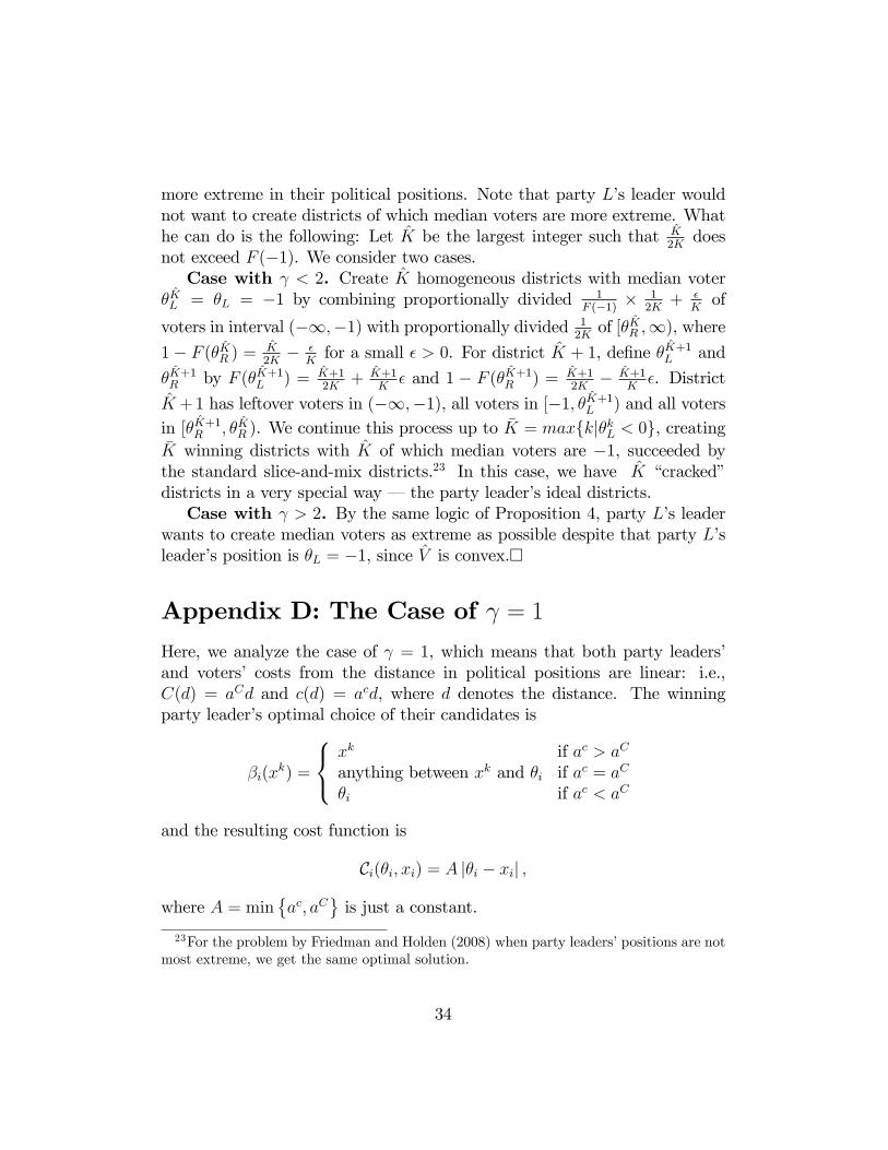
more extreme in their political positions. Note that party L�s leader wouldnot want to create districts of which median voters are more extreme. Whathe can do is the following: Let K̂ be the largest integer such that K̂

2Kdoes

not exceed F (�1). We consider two cases.Case with < 2. Create K̂ homogeneous districts with median voter

�K̂L = �L = �1 by combining proportionally divided 1F (�1) �

12K+ �

Kof

voters in interval (�1;�1) with proportionally divided 12Kof [�K̂R ;1), where

1� F (�K̂R ) = K̂2K� �

Kfor a small � > 0. For district K̂ + 1, de�ne �K̂+1L and

�K̂+1R by F (�K̂+1L ) = K̂+12K

+ K̂+1K� and 1 � F (�K̂+1R ) = K̂+1

2K� K̂+1

K�. District

K̂ +1 has leftover voters in (�1;�1), all voters in [�1; �K̂+1L ) and all votersin [�K̂+1R ; �K̂R ). We continue this process up to �K = maxfkj�kL < 0g, creating�K winning districts with K̂ of which median voters are �1, succeeded bythe standard slice-and-mix districts.23 In this case, we have K̂ �cracked�districts in a very special way � the party leader�s ideal districts.Case with > 2. By the same logic of Proposition 4, party L�s leader

wants to create median voters as extreme as possible despite that party L�sleader�s position is �L = �1, since V̂ is convex.�

Appendix D: The Case of = 1

Here, we analyze the case of = 1, which means that both party leaders�and voters� costs from the distance in political positions are linear: i.e.,C(d) = aCd and c(d) = acd, where d denotes the distance. The winningparty leader�s optimal choice of their candidates is

�i(xk) =

8<:xk if ac > aC

anything between xk and �i if ac = aC

�i if ac < aC

and the resulting cost function is

Ci(�i; xi) = A j�i � xij ;

where A = min�ac; aC

is just a constant.

23For the problem by Friedman and Holden (2008) when party leaders�positions are notmost extreme, we get the same optimal solution.

34

Thus, if party L is the gerrymanderer, (assuming �R = 1 and �L = �1)her payo¤ function from winning in district k is

~V kL (xk) =

8<:2A if xk � �12A��xk�� if � 1 � xk � 0

0 if 0 � xk

Thus, the optimal gerrymandering policy is to create as many districts with�1 � xk � 0 as possible, but otherwise, the gerrymanderer is indi¤erentwith how to allocate xks, otherwise. Thus, under determinacy, cases = 1and = 2 are similar to each other. When there is uncertainty, however,�pack-and-crack�would be recommended for the case of = 1 as in Owenand Grofman (1988).24

References

Bracco, E. (2013): �Optimal Districting with Endogenous Party Platforms,"The Journal of Public Economics, 104(C), pp. 1-13.

Besley, T., and I. Preston (2007): �Electoral Bias and Policy Choice: Theoryand Evidence,� The Quarterly Journal of Economics, 122(4), pp. 1473-1510

Coate, S., and B. Knight (2007): �Socially Optimal Districting: A Theo-retical and Empirical Exploration," The Quarterly Journal of Economics,122(4), pp. 1409-1471.

Dixit, A., and J. Londregan (1996): �The Determinants of Success of SpecialInterests in Redistributive Politics," The Journal of Politics, 58, pp. 1132-1155.

Dixit, A., and J. Londregan (1998): �Ideology, Tactics, and E¢ ciency inRedistributive Politics," The Quarterly Journal of Economics, 113 (2),pp. 497-529.

Ferejohn, J. A. (1977): �On the Decline of Competition in CongressionalElections," The American Political Science Review, 71(1), pp. 166-176.

24In order to maximize the number of xk+� in interval [�1; 0], xk should be concentratedat the central area of the interval.

35

Fiorina, M. P., J. C. Pope, and S. J. Abrams (2011): Culture War? TheMyth of a Polarized America. Boston: Pearson.

Friedman, J. N., and R. T. Holden (2008): �Optimal Gerrymandering: Some-times Pack, but Never Crack," The American Economic Review, 98(1), pp.113-144.

Gilroux, G. (2001): �Remap�s Clear Trend: Incumbent Protection,� CQWeekly, Nov. 3, pp. 2627-2632.

Gul, F., andW. Pesendorfer (2010): �Strategic Redistricting," The AmericanEconomic Review, 100(4), pp. 1616-1641.

Krasa, S., and M. Polborn (2015): Political Competition in Legislative Elec-tions, working paper.

Levendusky, M. (2009): The Partisan Sort: How Liberals Became De-mocrats and Conservatives Became Republicans. Chicago: Chicago Uni-versity Press.

Lindbeck, A., and J. W. Weibull (1987): �Balanced-Budget Redistribution asthe Outcome of Political Competition," Public Choice, 52 (2), pp. 273-297.

McCarty, N., K. T. Poole, and H. Rosenthal (2006): Polarized America: TheDance of Ideology and Unequal Riches. Cambridge, MA: MIT Press.

McCarty, N., K. T. Poole, and H. Rosenthal (2009): �Does GerrymanderingCause Polarization,�The American Journal of Political Science, 53(3), pp.666-680.

Osborne, M. J. (1995): �Spatial Models of Political Competition under Plu-rality Rule: A Survey of Some Explanations of the Number of Candidatesand the Positions They Take," The Canadian Journal of Economics, 28(2),pp. 261-301.

Owen, G., and B. N. Grofman (1988): �Optimal Partisan Gerrymandering,"Political Geography Quarterly, 7(1), pp. 5-22.

Puppe, C., and A. Tasnadi (2009): �Optimal Redistricting under Geograph-ical Constraints: Why �Pack and Crack" Does Not Work," EconomicsLetters, 105(1), pp. 93-96.

36

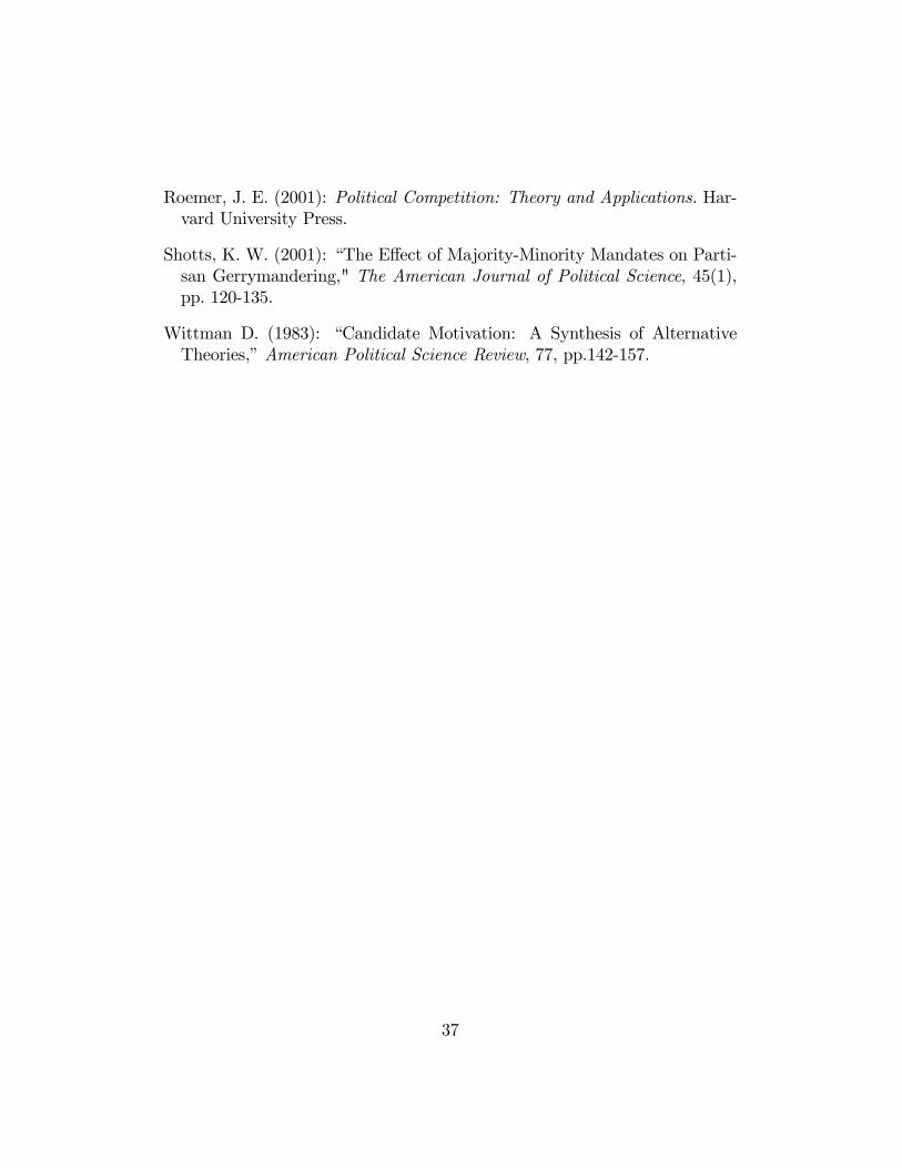
Roemer, J. E. (2001): Political Competition: Theory and Applications. Har-vard University Press.

Shotts, K. W. (2001): �The E¤ect of Majority-Minority Mandates on Parti-san Gerrymandering," The American Journal of Political Science, 45(1),pp. 120-135.

Wittman D. (1983): �Candidate Motivation: A Synthesis of AlternativeTheories,�American Political Science Review, 77, pp.142-157.

37

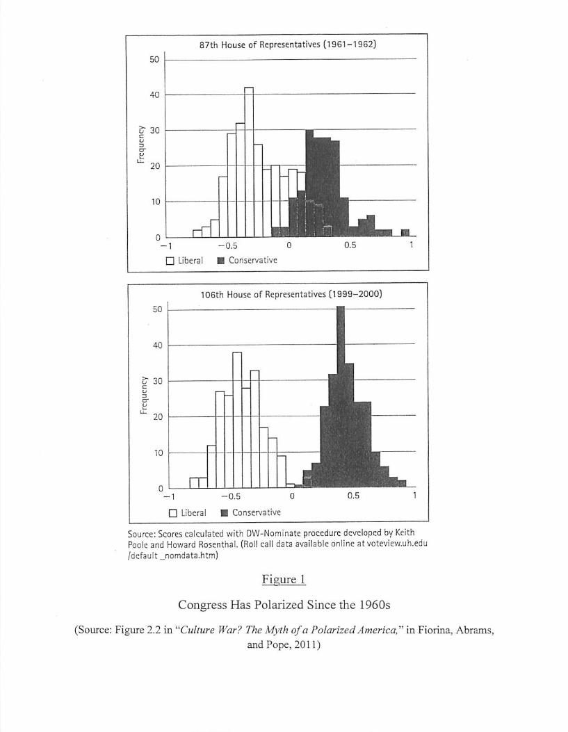
0 -1 𝑥𝑘(𝜋′) 𝑥𝑘(𝜋)

Δ Δ

𝑥�̃�(𝜋′) 𝑥�̃�(𝜋)

�̃�𝐿𝑘

𝛾 < 2

𝛾 = 2

𝛾 > 2

Figure 2

The Shape Winning Payoff Function

When 𝛾 ⋛ 0

Figure 3

The Winning Payoff Function When Corner Solutions Occur