1

Portfolio Selection with Transaction Costs and Jump-Diffusion

Asset Dynamics: A Numerical Approach

By Michal Czerwonko and Stylianos Perrakis1

Abstract

We derive the boundaries of the region of no transaction in a two-asset portfolio selection problem of an investor with isoelastic utility and with a finite horizon when the risky asset follows a mixed jump-diffusion process in the presence of proportional transaction costs. These boundaries are shown to differ from their diffusion counterparts in relation to the jump intensity and the risk premium, as well as the investor risk aversion coefficient. We use a discretization of the continuous time distribution that converges to jump-diffusion and a general numerical approach for iid risky asset returns in discrete time. We find that our approach converges efficiently to the continuous time results in cases where these results are known. Comparative results with a recent study on the same topic are presented and it is shown that the numerical algorithm has equally attractive approximation properties to the unknown continuous time limit.

(JEL G10, G11)

Current draft: January 2010

1 Both at Concordia University. They wish to thank George Constantinides and Sergey Isaenko for helpful

advice and comment. Financial assistance from Canada’s Social Sciences and Humanities Research

Council and from the Institut de Finance Mathématique (IFM2) is gratefully acknowledged.

2

1 Introduction

In this paper we extend the two-asset portfolio selection model under transaction

costs for an investor with an isoelastic utility function and finite horizon to a jump-diffusion

process for the risky asset with a jump component that may be, but is not necessarily,

lognormally distributed. We introduce a discrete time approximation to the continuous time

jump-diffusion process which converges weakly to it as the number of time subdivisions

increases. We also introduce an efficient numerical algorithm that allows the derivation of

the no transaction region of the portfolio selection model with a relatively small number of

discrete time intervals. Last, we show that our results are virtually identical to those of an

alternative indirect approach of the derivation of the no transaction region. In an appendix2

we present an exact solution to a problem examined in an older well-known study of

portfolio selection under simple diffusion, which had only derived an approximate solution.

We solve numerically the following problem, formulated in general terms. The

investor maximizes her derived utility of consumption, be it the consumption of the entire

wealth at the terminal finite date T or the consumption at all dates including the terminal

date. The investor is constrained to hold two assets, a riskless bond and a risky stock, with

the natural interpretation of an index. We denote the dollar holdings in the riskless bond as

x and the dollar holdings in the stock as y. The investor faces proportional transaction costs

at the rate k on transferring money from the stock account to the bound account and vice

versa but not on liquidating her bond holdings. The choice variable of the investor at each

discrete date t is the proportion of risky to riskless asset ( t t ty xλ ≡ ), which is a control

maximizing the derived utility of consumption. When we allow for consumption at

intermediate dates, the investor’s problem necessitates an additional control ( tc≡ ), which is

the optimal consumption at each discrete date t. In the discrete time setup we consider it a

natural extension of our model to allow for time but not for state dependent consumption.

Such an extension will not be attempted in this paper.

2 Available from the authors on request.

3

In spite of its simplicity, this problem has no analytical exact or even approximate solution

that we are aware of.3 Although portfolio selection in continuous time goes back to Merton

(1969, 1971), its practical implementation in the presence of transaction costs and with a

finite horizon is more recent and limited almost exclusively to simple diffusion.

Constantinides (1979) was the first one to prove that for an investor with an isoelastic utility

and in the presence of transaction costs the optimal policy consists of a compact no

transaction (NT) region in the form of a cone in which the investor does not trade, while she

trades to the nearest boundary of that region if the portfolio drifts outside the region.

Nonetheless, there were few attempts to implement these insights empirically, and almost all

of them were for diffusion processes. Even without transaction costs the presence of jump

components in the risky asset’s return distribution creates technical problems that prevent

exact analytical solutions to the problem of optimal portfolio choice for all but the simplest

cases. The addition of transaction costs when the investment horizon is finite is also a source

of difficulties even in the simple diffusion case, for which an approximate solution was not

derived till 2002.

Section 2 introduces our model in both its continuous and its discrete approximation

versions. Section 3 presents the numerical algorithm. Section 4 presents numerical results.

Section 5 summarizes and closes. In the remainder of this section we complete a literature

review of the portfolio selection rules in the presence of proportional transaction costs.

Constantinides (1979) proved an earlier conjecture in Magill and Constantinides

(1976) that the NT region is a cone composed of two boundaries and the optimal investment

policy is simple, i.e. it consists of trading to the closest boundary of this region if the risky to

riskless asset proportion falls outside the cone formed by the two boundaries.4

Constantinides (1986) was the first to present numerical results for the NT region. This

work considered an infinite horizon problem for a diffusion process. Under a simplifying

3 To our knowledge, the only study of portfolio selection under jump-diffusion and in the presence of

transaction costs derived recently and almost concurrently with this work is Liu and Loewenstein (2008).

We discuss this study further on in this section.

4 This result was proven in fairly general settings: not necessarily Markovian risky asset returns, additively or multiplicatively separable utility, transaction costs function positively homogenous of degree one in the investment decision, possibly adapted process for the bond account, the presence of dividends, finite or infinite investment horizon. See Propositions 5 and 7 in Constantinides (1979).

4

assumption of state and time independent consumption, Constantinides (1986) derived the

value function in a closed form; however, as the solution was composed of the value

function and two first order conditions, the derivation of the NT region required numerical

methods. Norman and Davies (1990) relaxed the simplifying assumption on consumption

policy by considering both time and state dependent consumption and obtained a closed

form solution composed of two ordinary differential equations. Their numerical results were

not qualitatively different from the ones in Constantinides (1986). As opposed to

Constantinides (1986) and Norman and Davies (1990), Dumas and Luciano (1991)

considered a portfolio choice of an investor who maximizes the derived utility of

consumption taking place upon the liquidation of the portfolio holdings at some future time

T. Dumas and Luciano (1991) considered a limiting case as the liquidation time T tends to

infinity. They assumed the discount factor to be endogenous to the problem, i.e. they solved

for the discount factor for which the partial derivative of the value function with respect to

time is zero. The results in that work differed from those of Constantinides (1986) first, in

that the NT region was found to be considerably wider; second, no shift towards the riskless

asset was found for increases in the transaction cost rate.

General theoretical results for portfolio selection in frictionless markets and for a

wide class of jump processes were presented by Duffie et al (2000). Liu at al. (2003)

extended that work and derived the Hamilton-Bellman-Jacobi (HBJ) partial differential

equation5 and the portfolio rules for such processes, but they provided numerical results only

in a special (and rather unrealistic) case of jump-diffusion, for a fixed jump size. The

portfolio rule was far apart from its diffusion counterpart, which is the Merton (1971) line.6

However, this result was obtained under the condition that in the presence of a jump

component the total volatility of the risky asset increases by the volatility of this component.

This is a less informative comparison than when the total volatility from both the diffusion

and jump components is kept constant, the case that we consider in our work.

5 The HBJ equation is a natural representation for the partial differential equation of the value function for the optimal investment problem. 6 The Merton line is an optimal risky to riskless asset proportion equal to

* */(1 )a a− , with

* 2( ) /(1 )a rµ δ σ= − − , the ratio of the risk premium to variance of the risky asset, for an infinite horizon

and frictionless trading for an agent with power utility and relative risk aversion δ .

5

In the presence of transaction costs Liu and Loewenstein (2002) considered the finite

horizon problem in continuous time for the two-asset simple diffusion case of

Constantinides (1986). The finite horizon makes the value function time-dependent and

prevents the solution of the HBJ equation. For this reason the authors replaced the fixed

horizon with a random terminal date, which occurs with the n-th passage of a Poisson

process.7 Since their later work provides a solution for a jump-diffusion process, we present

the Liu-Loewenstein methodology in some detail. There are two serious technical problems

with solving the HBJ equation in the presence of transaction costs: First, there are two free

boundaries varying through time; second, the time partial of the value function remains part

of the equation for a fixed investment horizon. The Liu-Loewenstein methodology explores

a randomization idea originally presented by Carr (1998) to produce an iterative sequence of

ordinary differential equations whose successive solutions converge to yield the solutions

for the value function and the boundaries of the no transaction region. Moreover, it was

shown that the solution for a random terminal date converges to the solution for a fixed

horizon equal to the expectation of this random quantity. In a later work Liu and

Loewenstein (2008) used the identical formulation for the jump-diffusion case and

considered the case where the jump component had a lognormal distribution, implying that

the portfolio value was not bounded away from zero at any time.8 They provided

approximate solutions for the fixed horizon case as the convergence value of successive

solutions of ordinary differential equations.9 In a later section we demonstrate that the

numerical results derived in this paper mirror the numerical results in Liu and Lowenstein

(2008) for the special case that they considered. .

Our numerical methodology has certain advantages with respect to the analytical

approaches. First, we are able to attack the finite-horizon problem directly, with a discrete

time dynamic programming method that converges to the continuous time case as the time

7 Under this stipulation, the horizon is Erlang distributed. Liu and Loewenstein (2002, 2008) also considered an exponentially distributed finite horizon, a case that is not relevant for the results of this paper. 8 Framstadt et al (2001) also examined portfolio selection under jump-diffusion in the presence of transaction costs in the infinite horizon case but do not provide any numerical results. 9Liu and Loewenstein (LL, 2008) demonstrated that the solution for a random Erlang-distributed horizon converges to the solution for a fixed horizon as the number of Erlang jumps increases. On the other hand, deriving numerical results for the LL semi closed-form solution becomes difficult for a large number of Erlang jumps.

6

partition becomes finer. Second, since our approach admits some flexibility in modeling for

the jump size distribution, we derive the solution also when the single-period jump size is

bounded away from zero, which allows the investigation of cases where it is optimal to

borrow in the presence of jumps. Last, the existence of an exact solution in the absence of

transaction costs makes it possible to assess the accuracy of the discrete time approximation

and extrapolate the results to the unknown case that we are attempting to solve.

2 Optimal Portfolio Policy under Proportional Transaction Costs

We present the dynamics in continuous time of the assets that we consider. We then

consider a discrete approximation that converges to the continuous time formulation as the

partition becomes finer. This allows us to formulate as a dynamic program the problem that

an agent faces while undertaking investment decisions in the presence of proportional

transaction costs.

2.1 Continuous time

First, we present the continuous time counterparts whose discretization we consider. The

bond holdings tx follow:

t tdx rx dt= , (2.1)

where r is the continuously compounded riskless rate. Our first case is the diffusion process

for the stock holdings ty :

t t t tdy y dt y dWµ σ= + , (2.2)

where tW is a standard Gauss-Wiener process and µ , σ are its instantaneous mean and

volatility parameters. In the second case we consider a mixed jump-diffusion process:

t d t d t t t t tdy y dt y dW K y dNµ σ− − −= + + , (2.3)

7

where ( )d Kµ µ ηµ= − and the last term is the jump component added to the diffusion. It is

assumed that the jump and diffusion components are independent. The variable Kt

represents the time-t realization of the random jump size K with K > -1 and N is an

independent Poisson counting process with intensity 0η > . The volatility of the diffusion

component of the stock process dσ is set so that the total volatility of the stock process is

equal to the volatility in the pure diffusion case, which implies ( )2 2 2

d K Kσ σ η σ µ= − + . In

our numerical work we apply two assumptions for the logarithm of the jump size: first, it is

distributed as ( )2,K K

N µ σ ; second, it is binomially distributed with the same parameters.

In continuous time under the asset dynamics given by (2.1)-(2.2) the objective is the

maximization of the function (2.4), where vτ represents the optimal portfolio revisions, the

additions to the stockholdings yτ net of transaction costs

{ }

( ) ,

( , , ) max + (1 ) , t t t T Tv t T

J x y t E U x k y Tτ τ∈

≡ − . (2.4)

Stock purchases (sales) vτ are financed by sales (purchases) of (1 )k vτ+ ( (1 )k vτ− ) of the

riskless asset, where k represents the transaction cost parameter, assumed for simplicity

equal for purchases and sales.10 The asset holdings after a revision become then y vτ τ+ and

x v k vτ τ τ− − .

We assume that this problem has as a solution a simple investment policy,

characterized by a NT region defined by two investment barriers τλ (buy boundary) and

τλ (sell boundary), [ , ]t Tτ ∈ limiting the proportiony

x

τ

τ

of the risky to riskless asset. The

investor transacts to the nearest boundary whenever [ , ]y

x

ττ τ

τ

λ λ∉ , while within the NT

region 0vτ = and the value function ( , , )J x yτ τ τ satisfies the following HBJ equation

(omitting the time subscripts)

10 It is assumed, in line with all previous studies, that there are no transaction costs for the riskless asset.

8

( ) 2 21[ ( , (1 ), ) ( , , )] 0

2t x K y yy

J rxJ yJ y J E J x y K t J x y tµ ηµ σ η + −+ + − + + + − = . (2.5)

The boundary conditions outside the NT region are given by

(1 ) , , (1 ) , x y x y

y yk J J k J J

x xλ λ+ = ≤ − = ≥ . (2.6)

As already noted, there are no closed form solutions for this problem, and even the

fact that the optimal solution is a simple policy has not been shown rigorously to the best of

our knowledge.11 For this reason we use a “control variate” technique: we solve a discrete

time problem that can be shown to converge to the continuous time solution under the asset

dynamics (2.2)-(2.3) in the absence of transaction costs. For such a problem we know from

Constantinides (1979) that the optimal investment policy is simple, and we derive an

algorithm by which it can be found. If by setting the transaction cost parameter to zero we

find that the approximation to the continuous time solution is adequate then we surmise that

the same thing is true for 0k > .

2.2 Discretization

We consider the following discrete approximation that converges weakly to (2.3),

expressed by Lemma 1 and proven in the appendix.12

Lemma 1: The following return process ( t tt t

t

yz

y

+∆+∆≡ ) is a valid approximation of (2.3):13

1 with probability 1

1 with probability

d dt t

t t tz

K t

µ σ ε η

η+∆

+ ∆ + ∆ − ∆=

+ ∆ , (2.7)

11 Framstadt et al (2001) demonstrate it for an infinite horizon, while Liu and Lowenstein (2008) use a formulation with a random horizon. 12 See also Oancea and Perrakis (2009). 13 The approximation (2.4) converges weakly to (2.3), in the sense that the expectation of any continuous function of the random stock return at some future time taken with respect to the discrete process converges to the expectation of that same function taken with the continuous time limit of the process. This is the appropriate convergence criterion for our problem.

9

where ε is a random variable with a given distribution of mean 0 and variance 1 that can be

anything. This return process is a mixture of the diffusion and jump components with

corresponding probabilities 1 tη− ∆ and tη∆ .14

In our numerical work we use for the distribution of ε a trinomial distribution

described in a later section. We lay out further details of our discretization in Section 3 and

in the appendix.

Under proportional transaction cost, the bond and stock accounts dynamics are:

( )

( )

1

1 1

t t t t

t t t t

x x v k v R

y y v z

+

+ +

= − −

= +

, (2.8)

where tv denotes the time-t investment decision, the dollar amount net of transaction costs

by which the investor changes her risky asset account. The investor solves the following

problem of maximizing the expected utility of the terminal wealth net of transaction costs:

{ }

( ) ,..., 1

max + (1 ) , t T Tv t T

E U x k y Tτ τ∀ ∈ −

− , (2.9)

s. t. (1 ) 0t t

x y k+ − > and (1 ) 0t tx y k+ + > (solvency constraints), where vτ is the time-τ

investment decision. As with the continuous time case, the solution to the investor’s

problem is a pair of boundaries of the NT region. We denote the buy and sell boundaries by

tλ and t

λ , respectively and by tλ the time-t risky to riskless asset proportiony

x

τ

τ

. Note that

the NT region is a convex subset of the solvency region characterized by the above two

boundaries.15 This effectively precludes borrowing for lognormally distributed jumps since

the investor will face a positive likelihood of ruin.

14 Alternatively, (2.7) can be replaced by a convolution of the diffusion and jump components. The asymptotic properties, however, remain the same. Our discrete time algorithm follows the mixture. 15 When both x and y are positive, the solvency constraints are trivially satisfied due to limited liability. The first constraint ensures the positive net worth for borrowing, the second for selling the stock short. Under a positive risk premium and risk aversion, it is never optimal to sell short the risky asset.

10

The most frequently used approach to solve for (2.7) is the dynamic programming

formulation:

( ) ( )1 1, , Max , , 1t

t t t t tv

V x y t E V x y t+ += + (2.10)

with the boundary conditions:

( ) ( ), , (1 ) ,T T T TV x y T U x k y T= + − . (2.11)

The isoelastic utility function ( ) /T

Wα

α , where 1α δ= − , with δ denoting the relative risk

aversion (RRA) coefficient, results in a concave and homogenous of degree α in its

arguments value function (2.10)-(2.11), as was shown in Constantinides (1979). This is also

the approach that we use to solve the problem at hand. As we argue later, for the applied

risky asset discrete-time dynamics (2.7) and the resulting state dynamics for the problem

(2.10), applying (2.9) will yield an easy to apply and precise numerical solution.

A central role in our analysis will be played by two functions deriving the indirect

(not necessarily maximized) utility for purchase and sale of the risky asset, respectively

( ).J and ( ).J , which we define as:

( ) ( ) ( ){ }

( ) ( ) ( ){ }

1

1

, , , (1 ) , , 1

and

, , , (1 ) , , 1

t t t t t t t t t

t t t t t t t t t

J x y v t E V x k v R y v z t

J x y v t E V x k v R y v z t

+

+

= − + + +

= − − + +

. (2.12)

To increase the proportion of the risky to riskless asset to some new proportion tλ ( 0tv > ),

the investment decision is:

(1 ) 1t t t

t

t

x yv

k

λ

λ

−=

+ +. (2.13)

Substituting this last quantity into the first line of (2.10) yields:

11

( ) ( ) 1, , , (1 ) , , 1(1 ) 1 (1 ) 1

t tt t t t t t

t t

zRJ x y t x k y E V t

k k

α λλ

λ λ+

= + + +

+ + + + , (2.14)

where we used the homothetic property of the value function to take the term outside the

expectations operator. A similar argument for the stock sale yields:

( ) ( ) 1, , , (1 ) , , 1(1 ) 1 (1 ) 1

t tt t t t t t

t t

zRJ x y t x k y E V t

k k

α λλ

λ λ+

= + − +

− + − + . (2.15)

It can be shown that maximizing (2.14) and (2.15) with respect to tλ yields, respectively the

buy and the sell boundary of the NT region tλ andt

λ .16 Since it is apparent that the terms

in powers α are inconsequential positive quantities, we have the following program solving

for tλ andt

λ :

( )

( )

arg max ,

and

arg max ,

t

t

t t

t t

V t

V t

λ

λ

λ λ

λ λ

=

=

, (2.16)

where:

( )

( )

1

1

, , , 1(1 ) 1 (1 ) 1

and

, , , 1(1 ) 1 (1 ) 1

t tt t

t t

t tt t

t t

zRV t E V t

k k

zRV t E V t

k k

λλ

λ λ

λλ

λ λ

+

+

= +

+ + + +

= +

− + − +

. (2.17)

16An induction proof is in the Appendix to Genotte and Jung (1994), itself an application of the general result in Constantinides (1979) to the CRRA utility function.

12

If the NT region exists, the program (2.16)-(2.17) will always yield a solution since the

value function is strictly concave.

We may now formulate compactly the investor’s dynamic problem with the

inclusion of the optimal investment policy:17

( )

( ) ( )

( )

( ) ( )

t

1 t

t

(1 ) , for

, , , , 1 for

(1 ) , for

t tt t

ttt t t t t t

t tt t

x k y V t

V x y t E V x R y z t

x k y V t

α

α

λ λ λ

λ λ λ

λ λ λ

+

+ + <

= + ≤ ≤ + − >

. (2.18)

3 Numerical Analysis

We describe our numerical approach that is based on forward induction. A critical step in

this approach consists of an efficient incorporation of already known solutions to the

problem at all future dates. Further, we present details of the discretization of the risky asset

dynamics.

3.1 Forward induction

To solve for the program (2.16)-(2.17) we apply the direct approach (2.9). This is a

forward-inductive approach, that yields ( ),tV tλ and ( ),tV tλ as continuous functions of tλ ,

resulting in flexible modeling. This admits the derivation of the NT region by reliable

optimization routines resulting in highly accurate estimates. In general, for the current

17 In an appendix (available form the authors on request) we show by using our formulation that the well-known study by Genotte and Jung (1994) for portfolio selection under diffusion contains systematic errors that may distort the results.

13

setting, we may write the value function as the expectation of the terminal utility of wealth

with respect to the underlying probability space:18

( )[ ]

( ), , , 1

, , max (1 ) Pr( )t t T j T j j

v t Tj

V x y t U x k yτ τ

ω∀ ∈ −

= + −∑ , (3.1)

where j

ω represents a path j for a given discrete-time probability space, and ,T jx and ,T j

y

have been derived for the filtration of a given probability space and the optimal investment

decisions at all dates τ = t, t + 1, … , T – 1. In particular, (3.1) applies to the program (2.16)-

(2.17) with appropriate quantities substituted for ,t t

x y .

Since we use a (multidimensional) tree to represent the process of the risky asset,

equation (3.1) appears to be difficult to solve in numerical work for more than a few time

periods. The difficulty stems from the fact that the number of paths grows exponentially in

time partition. To deal with this difficulty, in the following paragraphs we present a

recursive model which efficiently aggregates the paths of the state variable τλ ,

1,..., 1t Tτ = + − . As we will show, exploiting the fact that the ratio y

x

τ

τ

is the sole state

variable, the homothetic property of the value function and the recombination property of

the assumed discretization of the risky asset dynamics will allow us to aggregate the states at

each forward step.

Assume that the boundaries of the NT region τλ and τλ were found for all times

1,..., 1t Tτ = + − . Given this information set, we define the indirect but not necessarily

maximized utility for a portfolio consisting of $1 in the riskless and $ tλ in the risky asset at

time t for the probability space as defined in (3.1) and for the future optimal portfolio

restructuring:

( ) ( ) { }, , 1,..., 11, , (1 ) Pr( ) | ,t T j T j j t T

j

J t U x k y τ τ τλ ω λ λ

= + −≡ + −∑ . (3.2)

18 The idea of solving for the NT region by forward induction in numerical work was first presented in Boyle and Lin (1997). However, their numerical approach considered the first order condition on the terminal utility, which was suitable to solve the problem only for a limited number of periods.

14

By (2.16)-(2.17) and (3.2) it is clear that we have:

( ) ( ){ }

( ) ( ){ }

arg max 1 1 1, ,

and

arg max 1 1 1, ,

t

t

t t t

t t t

k J t

k J t

α

λ

α

λ

λ λ λ

λ λ λ

−

−

= + +

= − +

. (3.3)

We partition the time-τ paths of the state variable τλ into two types: the first type

includes those paths which remain inside the NT region, and the second type includes the

paths that fall outside this region and are traded to the nearest boundary τλ or τλ by virtue

of the simple investment policy. The first type of paths presents no particular problem since

inside the NT region the state variable will follow the recombination pattern of a given

lattice. To see that, consider that in this case the time-τ portfolio holdings are ( )ˆ,t

tR Zτ

τλ− ,

with the cumulative stock return up to time τ 1ˆ t

i t iZ zτ

τ−

= +≡ Π which implies ˆ

t t

Z

R

ττ τ

λ λ−

= , with

the associated probabilities resulting from the ( tτ − )-period convolution of the one-period

distribution of the risky asset with itself.

For the second type of paths, namely those for which the simple investment policy

stipulates a trade to the nearest boundary of the NT region, at each time τ we derive a single

number, the contribution of these paths to the terminal derived utility ( Jτ≡ ∆ ). As we will

demonstrate, the quantity Jτ∆ will subsume all the relevant past and future path information

as of time-τ. We elaborate below on the derivation of Jτ∆ ; here we define it implicitly by

( ) ( ) ( )( )1

1

, ,

1 1

ˆ ˆ1, , Pr 1TNT

T t

t T l t T l

t l

J t J Z R k Zα

ττ

λ α λ−

− −

= + =

= ∆ + + −∑ ∑ , (3.4)

15

where the second summation is over the TN paths which remained inside the NT region at

each and every time τ, 1,..., 1t Tτ = + − , with ( )Pr . denoting time-t probabilities of the

terminal states of the risky asset.19

To aggregate the time-τ paths outside the NT region to Jτ∆ defined above, we use

the homothetic property of the value function and the fact that we already solved for the

value function ( )1, ,V τλ τ and ( )1, ,V τλ τ , 1,..., 1t Tτ = + − by maximizing (3.3). To

demonstrate that there exists an aggregation that yields (3.2), the derived utility that

subsumes all the relevant path information, we use the following result, proven in the

appendix.

Lemma 2: The contribution Jτ∆ of all time-τ paths outside the NT region to the time-t

derived utility of terminal wealth as defined by (3.4) is the following:

( ) ( )1, , 1, ,J X V X Vτ τ τ τ τλ τ λ τ ∆ = + , (3.5)

where ( ) ( )( )

,

,

1

ˆ1ˆPr1 1

tnt i

i

i

R k ZX Z

k

τ

ατ

ττ τ

τ

λ

λ

−

=

+ +=

+ + ∑ and

( )( )( )

,

,

1

ˆ1ˆPr

1 1

tnt j

j

j

R k ZX Z

k

τ

ατ

τ

τ τ

τ

λ

λ

−

=

+ −=

− + ∑ , where ,

ˆiZτ and ,

ˆjZτ are respectively the stock

returns resulting in the portfolio proportion τλ below or above the NT region, ( )Pr . are the

time-t probabilities of these returns, and we denote the time-τ number of ,ˆ

iZτ ’s ( ,ˆ

jZτ ’s) by

nτ ( nτ ). Note that these probabilities may be derived by simply following the

recombination pattern of a given lattice. The terms under the power of α are time-τ dollar

values of the bond account after transacting to a given boundary of the NT region.

With the use of Lemma 2, we rewrite the maximization problem (3.3) as follows:

19 In our numerical work, we use the fact the lattice is recombining inside the NT region, which implies that at the terminal date we have nodes rather than paths.

16

( ) ( ) ( )( )

( ) ( ) ( )( )

11

, ,1 1

11

, ,

1 1

ˆ ˆarg max 1 1 Pr 1

and

ˆ ˆarg max 1 1 Pr 1

T

T

NTT t

t t T l t T l

t l

NTT t

t t T l t T l

t l

k J Z R k Z

k J Z R k Z

αα

ττ

αα

ττ

λ λ α λ

λ λ α λ

−− − −

= + =

−− − −

= + =

= + + ∆ + + −

= − + ∆ + + −

∑ ∑

∑ ∑

, (3.6)

where the second summation is over the TN recombined paths which remained inside the

NT region at each and every time τ, 1,..., 1t Tτ = + − .

Now we can describe the major steps of our numerical solution. Take a candidate

solution tλ for either maximization problem in (3.3) and proceed forward with the lattice.

At each time τ derive the terminal contribution Jτ∆ of all paths outside the NT region by

(3.5). Delete these paths from the lattice and repeat the process till 1Tτ = − is reached.

Since it is apparent that equation (3.6) yields the derived utility as a continuous function of

tλ , the maximization problem can be passed to optimization routines present in many

software packages such as Matlab. Except for possible numerical errors, the formulation

(3.9) yields the exact solution for the NT region for a given discretization approach. This

algorithm executes in short time even for the large number of nodes in a one-period lattice

that we use to approximate a jump-diffusion process, since a limited number of nodes

remains inside the NT region at any time τ.

With the use of Lemma 2, we may also state the first order conditions (FOC) for the

problem in a closed form.20. By substituting from (3.5) into (3.6), differentiating and

simplifying, we have the following FOC:

20 Boyle and Lin (1997) formulated a similar approach for solving a simpler problem but did not reach a closed form solution and so solved the problem for a very small number of periods

17

( )

( )

( )

1,

,

1 1

1,

,

1 1

,

,

ˆ(1 ) ( )ˆPr ( , , )( , , ) ( ) 1

ˆ(1 ) ( )ˆPr ( , , )( , , ) ( ) 1

ˆ(1 ) ( )ˆPr ( , , )( , , ) ( ) 1

nTi

i t

t i t

nTj

j t

t j t

T l

T l t

t

k Z c kG Z i

i c k

k Z c kG Z j

j c k

k Z c kZ T l

T l c k

τ

τ

τατ τ

τ

τατ τ

τ

α

ϕ λ τϕ λ τ λ

ϕ λ τϕ λ τ λ

ϕ λϕ λ λ

−

= + =

−

= + =

+−

+

−+ −

+

−+ −

+

∑ ∑

∑ ∑

1

TN

l=

∑

(3.7)

where ( ) ( )1, , /( 1 1)G V kα

τ τ τα λ τ λ= + + , ( )(1, , ) /( 1 1)G V kα

τ τ τα λ τ λ= − + ,

,ˆ( , , ) (1 )t

t t ii R k Zτ

τϕ λ τ λ−= + + , ,ˆ( , , ) (1 )t

t jj R k Zτ

τϕ λ τ λ−= + − ,

,ˆ( , , ) (1 )T t

t t T lT l R k Zϕ λ λ−= + − and c(k) is set equal to 1 + k and 1 – k, respectively for the

buy and sell boundary of the NT region. In principle, (3.7) may be solved to yield the

boundaries of the NT region instead of brute-force maximization of (3.6); however, this

approach doesn’t appear to have numerical advantages.

3.2 Numerical estimation

To solve for the NT region for the diffusion case, we approximate the stock dynamics by the

Kamrad and Ritchken (1991) trinomial model. For the jump-diffusion case we use a

multinomial approximation. When the jump size is lognormally distributed, we

approximate the diffusion component by the trinomial model with the mean and variance

implied by (2.3) with the probabilities adjusted by the factor1 tη− ∆ . To approximate the

jump component, we space 3m > states within the span ±6σK by the same distance in the

log scale as in the trinomial model and derive the probabilities as the normalized to 1

densities implied by the distribution of the jump component K. These probabilities are

adjusted by the factor tη∆ . In the final step, the adjusted trinomial probabilities are added to

the adjusted three central probabilities of the jump component. When the jump size is

binomially distributed, we search for a trinomial model for the diffusion component such

that its span multiplied by a natural number greater than one yields the span of the jump

component, a feature that is necessary for the resulting composite lattice to recombine. We

then combine both components as before. We lay out further details for our discretization in

the appendix.

18

A straightforward discretization may lead to errors in terms of the mean and

volatility of the discretized process relative to similar parameters of the continuous-time

process. We solve this problem by adjusting the mean and the variance for the discretized

process so that these parameters net of discretization errors exactly match the true ones. As

shown in the appendix, these adjusted parameters may be found easily by solving a set of

two non-linear equations. It is also shown that the adjusted parameters are close to the true

ones.

To derive the NT region, we start at t T t= − ∆ and move recursively backward

while using the forward induction (3.1)-(3.2) to solve the problem at each time t. The

function (3.9) is derived and passed to an optimization routine, which derives its

maximizing arguments. We use a time partition of 250 for one calendar year, which

approximately corresponds to daily portfolio revisions.

3.3 The analysis for a frictionless market

As was shown in Merton (1969) and Liu at al. (2003) among others, the optimal portfolio

policy for a diffusion or jump-diffusion process in continuous time without transaction costs

for an isoelastic utility function is myopic. This is not generally true for a given time

partition and varying horizon length for a discretized process. On the other hand, for any

investment horizon length and for a successively finer time partition our discrete-time

results clearly tend to their continuous-time counterparts, an expected result under the weak

convergence criterion. Here we reproduce the Liu and Loewenstein (2008) result for a

mixed process under an exponentially distributed investment horizon. They derive the

following function:

2 2 1( ) ( [ ]) / 2 [(1 ) /(1 )]r r E K E K

δρ θ θ µ η θ σ δ η θ δ−= + − − − + + − (3.7)

Liu and Loewenstein (2008) showed that the above function is strictly concave in θ ≤ 1 , and

its unique maximizer θ* yields the optimal risky to riskless asset proportion as θ*/(1 – θ*).

In our case a program deriving the optimal portfolio proportions for a finite horizon

in discrete time results from setting the transaction cost rate k equal to zero in (2.16)-(2.17)

and maximizing the terminal utility of wealth in the risky to riskless asset proportion. Note,

19

however, that since at each time period the portfolio is traded to reach this same ratio, which

is the sole state variable for the problem, the solution would be the same as for the one-

period problem with the given discretization. To take the advantage of the convergence of

our discretization to the continuous-time distribution, we successively increase the time

partition and solve the frictionless case for the terminal distribution. This approach will

allow the verification of the precision of our approach since the continuous-time results are

easy to derive.

4 Results

We focus the presentation of our main results on the differences between the diffusion and

jump-diffusion cases. Our base case uses the following set of parameters: total volatility σ

of 18%, risk premium of 6%, jump intensity η of 0.5, jump volatility σK of 7%, transaction

costs rate k of 0.5%, relative risk aversion (RRA) δ of 3 and logarithm of the expected jump

size µK of -2%. In all presented cases the time step, ∆t is 1/250.

First, we estimate the results for the frictionless markets (k = 0) for the diffusion (η =

0) and for the mixed process (η = 0.5). With our discretization the Merton line for the

diffusion is 1.6130, compared to the continuous-time optimal risky to riskless asset

proportion of 1.6129. Our discrete and continuous-time jump-diffusion counterparts

respectively are 1.6081 and 1.6084 indicating good convergence properties of our

discretization approach. We see that the optimal investment policy is little different in both

cases, which provides an indication for the results in the presence of transaction costs.

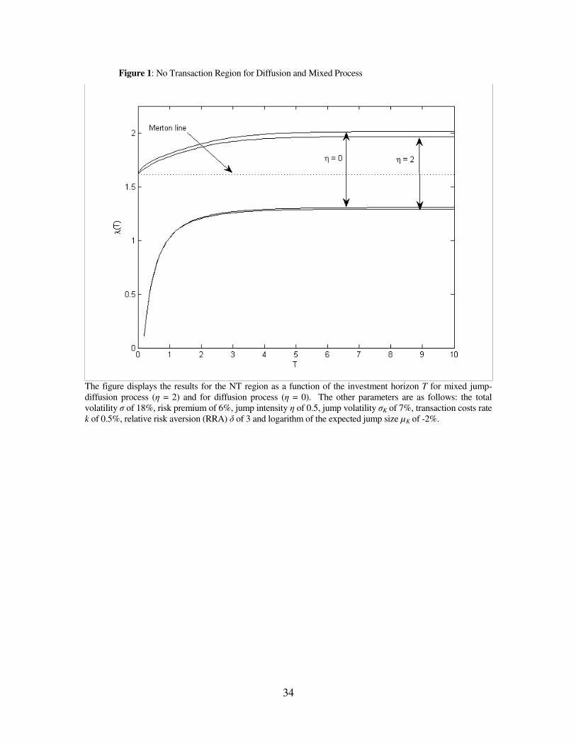
[Fig 1 around here]

20

Figure 1 displays the NT region for the above parameters for k = 0.5% and for jump

intensities η equal to 0 (diffusion) and 2.21 In Figure 1, we may also clearly observe the

convergence of the NT region boundaries to constant levels as the horizon length increases

for a given set of parameters.

[Table 1 around here]

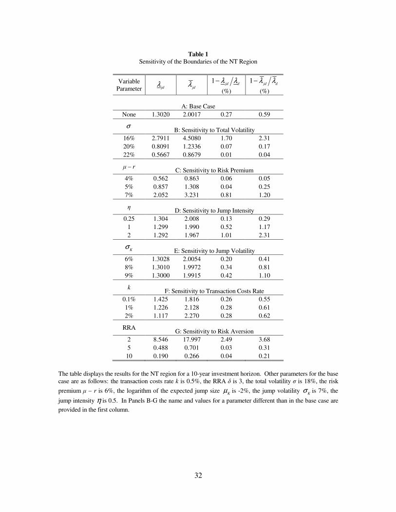
Table 1 presents the numerical results for our base case, as well as for variation in all

parameters except for the logarithm of the expected jump size µK whose changing brought

little variation in the results since the diffusion component is compensated for its values to

keep the total mean constant. In Panel B, where we increase the total volatility without

changing the volatility of the jump component, we observe a convergence of the results for

the mixed and pure diffusion processes. In Panels C-E we observe an increasing divergence

between the results for the mixed and pure diffusion processes corresponding respectively to

increases in the risk premium, jump intensity and jump volatility. From the results in Panel

F, there appear to be little effect of varying the transaction cost rate for the relation between

the results for the mixed and pure diffusion processes. Last, the results in Panel G for

increasing the risk aversion coefficient display a convergence between the mixed and pure

diffusion processes. To put the overall differences between the two considered processes in

perspective, we focus on the top line of Panel G, where for the RRA of 2 we observe the

highest relative divergence between the results in Table 1. This highest divergence for our

choice of parameters translates into the difference in the risky asset holdings of the order of

0.1 and 0.2% proportionally to the total wealth, respectively at the buy and sell boundary of

the NT region.

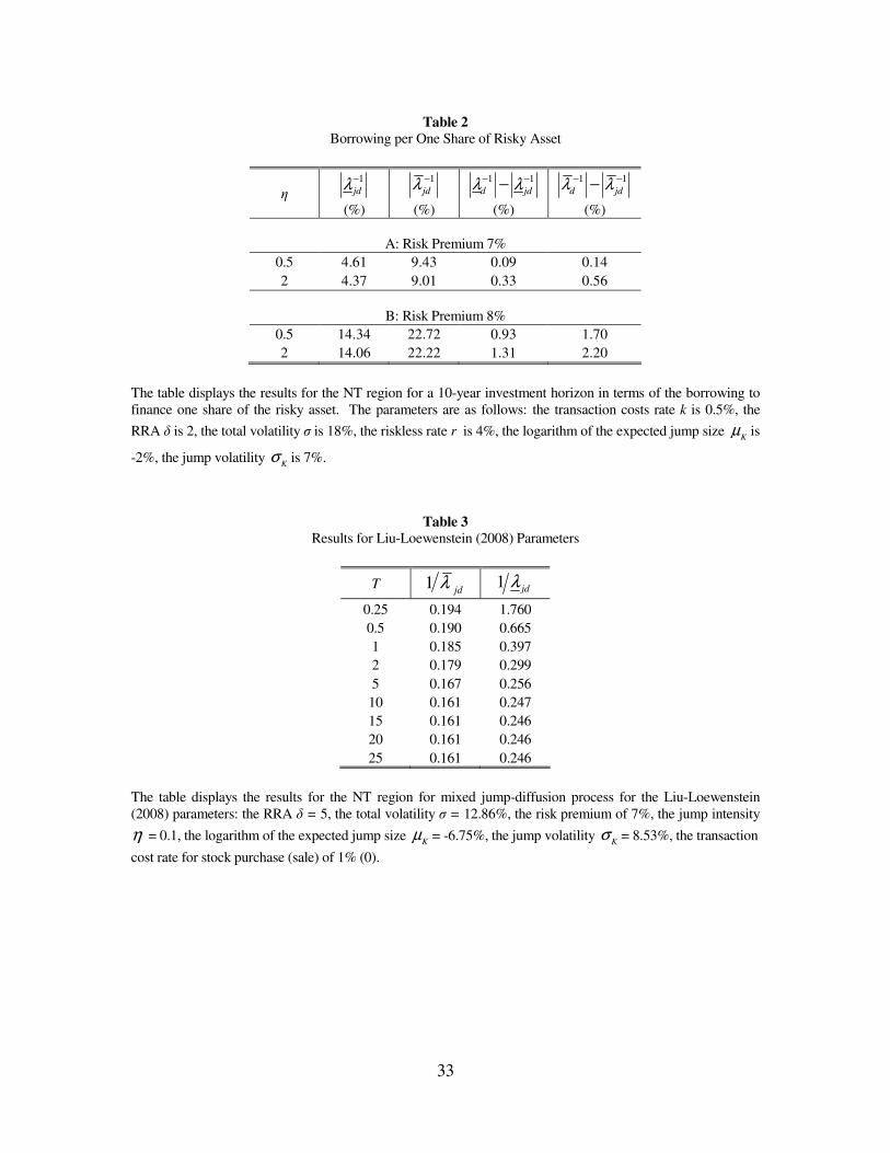
[Table 2 around here]

21 For our base case (η = 0.5), the graphs of the NT region for the diffusion and mixed process almost coincide.

21

For the parameter values when it is optimal to borrow for the bounded jump size,

instead of presenting the boundaries of the NT region in terms of the risky to riskless asset

proportions, which are negative in this case, we present more intuitively our results in terms

of borrowing per one share of the risky asset. In other words, the investor borrows the

indicated quantity to purchase one share of the risky asset, with the remainder of financing

coming from her own wealth. It is clear from Table 2 that the borrowing varies significantly

with the risk premium while the impact of the jump intensity η is relatively small. In terms

of the differences in the risky asset holdings in proportion to the total wealth between the

mixed and pure diffusion processes, the bottom line in Panel B, for which these differences

are the largest may be translated into the differences of 1.8 and 3.7%, respectively at the buy

and sell boundary of the NT region.

From the results in Table 1 it appears, therefore, that for our choice of parameters,

when there is no borrowing the optimal policy for the mixed process is very similar to the

pure diffusion case as underlined by the highest 0.2% difference for the risky asset holdings

in proportion to the total wealth. The differences in the optimal policy between the two

cases appear to grow when it is optimal to borrow, as evidenced in Table 2.

An open question of our work is the accuracy of our discrete time numerical

algorithm in approximating the continuous time solution in the presence of transaction costs.

Unfortunately there are no closed form expressions for the NT region for the jump-diffusion

problem (or, for that matter, for simple diffusion) when the investment horizon is finite. For

this reason we compare our results to those of a different approximation to the exact

solution, by Liu and Lowenstein (2008). Their approximation to the continuous time

solution is in the form of an Erlang-distributed horizon that produces a sequence of ordinary

differential equations, whose successive solutions converge to the value function and NT

region of the fixed-horizon jump-diffusion case.

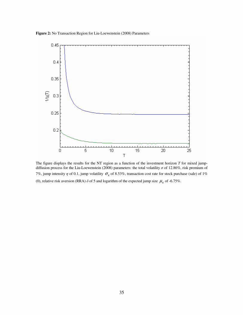
[Fig 2 around here]

22

Figure 2 and Table 3 show the NT region for the jump-diffusion case evaluated with our

algorithm for the parameter values used by Liu and Lowenstein (LL, 2008). We follow the

presentation in that latter study, i.e. we display the reciprocals of the NT region boundaries

as defined in this paper with the following set of parameters: the RRA δ of 5, the total

volatility σ of12.86%,22 the risk premium of 7%, the jump intensity η of 0.1, the logarithm

of the expected jump size Kµ of -6.75%, the jump volatility Kσ of 8.53%, the transaction

cost rate k for stock purchase (sale) of 1% (0).

[Table 3 around here]

Although the exact numerical values of LL are not available, it is clear that our

diagram is virtually identical to the corresponding LL Figure 6. Hence, there is reason to

believe that our numerical algorithm provides equally good convergence and approximation

properties to the “true” continuous time solution as the alternative approximation through

the Erlang-distributed horizon of the Liu-Lowenstein (2002, 2008) approach.

22 This value of the total volatility corresponds to the value of the diffusion component of 12.39%.

23

5 Concluding Remarks

We presented an efficient numerical solution to the problem of deriving the NT region in a

discrete-time finite-horizon case for iid risky asset returns. The solution to our main

research question indicates that the major factor driving the NT region for the mixed process

apart from its diffusion counterpart is the jump intensity. It remains an empirical question

whether the jump intensity estimated from market data would lead to major changes in

portfolio rules compared to the simple diffusion case. Further, an empirical study may

examine relative gains or losses in derived utility resulting from the adoption of either

investment policy and tested with the observed paths of an index.

A factor that may modify the influence of the jump intensity on the NT region is

intermediate consumption. We hypothesize that with intermediate consumption even

relatively low jump intensity may lead to portfolio rules for the mixed process relatively far

apart from its diffusion counterpart. The reason for this conjecture is the plausibility that the

risk aversion will sway an agent from holding the risky asset given that a large proportion of

the risky asset in the agent’s portfolio may lead to low consumption states at intermediate

dates in the presence of jumps. The verification of this conjecture should be a topic of

future research.

24

Appendix

Proof of Lemma 123

The characteristic function of the terminal stock price at time T for a $1 initial price under

the jump-diffusion process (2.3) is

2 2

0

2 2

( )( ) exp( )exp( ) [ ( )]

2 !

exp( )exp[ ( ( ) 1)],2

NNd

JD d J

N

dd J

T Ti T T

N

Ti T T

ω σ ηϕ ω ωµ η ϕ ω

ω σωµ η ϕ ω

∞

=

= − −

= − −

∑ (A.1)

where ( )J

ϕ ω is the characteristic function of the jump distribution. The first exponential

corresponds to the diffusion component and the second to the jump component.

The characteristic function of the discretization (2.7) is

( ) ( ) (1 )[exp( ) ( )],J d d

t t i t tεϕ ω η ϕ ω η ωµ ϕ ωσ= ∆ + − ∆ ∆ ∆ (A.2)

where ( )εϕ ω is the characteristic function of ε .24 Since the distribution of ε has mean 0

and variance 1, we have

2

[ ] 0 (0)

[ ] 1 (0)

E i

E

ε

ε

ε ϕ

ε ϕ

′= =

′′= = −

By the Taylor expansion of ( )εϕ ω , we get

2 2

2 2( ) ( ) (1 ) exp( )[1 ( )] ,2

dJ d d d

tt t i t th t

ω σϕ ω η ϕ ω η ωµ ω σ ωσ

∆= ∆ + − ∆ ∆ − + ∆ ∆

23 The proof is similar to that of Theorem 21.1 in Jacod and Protter (2003). 24 If, instead of (2.2) we have a convolution of the diffusion and jump components then the characteristic

function becomes ( ) ( ( ) 1 )[exp( ) ( )]J d d

t t i t tεϕ ω η ϕ ω η ωµ ϕ ωσ= ∆ + − ∆ ∆ ∆ . The multiperiod

convolution, however, still converges to (A.3).

25

where ( ) 0h ω → as 0.ω → The multiperiod convolution has the characteristic function

/( )T tϕ ω ∆ . Taking the limit, we have

( )

/

0

2 22 2

0

2 2

[ ( )]lim

exp ln( ( ) (1 ) exp( )[1 ( )]lim2

exp ( ) 12

T t

t

dJ d d d

t

dJ d

tTt t i t th t

t

TT i T

ϕ ω

ω ση ϕ ω η ωµ ω σ ωσ

ω ση ϕ ω ωµ

∆

∆ →

∆ →

=

∆∆ + − ∆ ∆ − + ∆ ∆

∆

= − + −

(A.3)

after applying l’Hospital’s rule. (A.3) is, however, the same as (A.1), the characteristic

function of (2.3), and Levy’s continuity theorem25 proves the weak convergence of (2.4)

to (2.3), QED.

Proof of Lemma 2

The lemma may be demonstrated very simply by induction. Without loss of generality, in

our proof we consider only the portfolio adjustments to the lower boundary of the NT region

τλ and the resulting quantity Xτ . The inclusion of the adjustment to the other boundary τλ

follows easily by extension. Consider 2t T= − . We have

( ) ( )( )1

1 1

1

1, , 1 1m

T s T s

s

V T p R k zα

λ α λ−− −

=

− = + −∑ , where ip is the probability of a one-period

stock return iz , 1...s m= . With the use of the lemma, we have:

( )

( )( )( )

121

1 1

1 11

11

1 1

Tn mT i

T i s T s

i sT

R k zJ p p R k z

k

α

αλα λ

λ

−−−

− −= =−

+ +∆ = + + + +

∑ ∑ , (A.4)

where the first summation results from the definition of Xτ , 1Tτ = − , and 1 0Tm n −≥ ≥ .

By the homothetic property which in this simple case collapses to multiplying terms under

the same power, (3.6) yields the same result we would get from equation (3.2) by

considering each path separately.

25 See for instance Jacod and Protter (2003), Theorem 19.1.

26

Consider any time t. Assume that the lemma holds at 1τ + . At time τ we have:

( ) ( )( )

( )( )

( ),

1 1

ˆ ˆ1 1ˆPr , , 1, ,1 1 1 1

n nt i t i

i

i i

R k Z R k ZJ Z V X V

k k

τ τ

τ τ τ τ τ

τ τ

λ λλ τ λ τ

λ λ= =

+ + + +∆ = ≡

+ + + + ∑ ∑ . (A.5)

When we apply one forward inductive step to the quantity above we get:

( )( )

( )

( )( )

( )

( )

1

1

1 1

1

1 1

11 1 1

1

11, , 1

1 1

11, , 1

1 1

, , 1

nk

k

k

n nj

j

i j

m n n

s s

s

R k zp V

k

R k zJ X p V

k

p V R z

τ

τ τ

τ τ

α

ττ

τ

α

τ

τ τ τ

τ

τ

λλ τ

λ

λλ τ

λ

λ τ

+

+

+ +

+= +

+= = +

− −

=

+ + + + + + + −

∆ = + + − + +

∑

∑ ∑

∑

, (A.6)

where the first two summations in square brackets consider these one-period paths that are

outside the NT region by using the induction hypothesis, and the third one considers these

paths which remain inside this region, with kz ’s, j

z ’s and sz ’s denoting appropriate one-

period returns and m denoting the number of one-period returns in a given lattice. Since, by

the definition of Xτ it is apparent that equation (A.4) considers all the relevant path

information, continuing forward until the terminal date T is reached will reproduce the

definition (3.2) for the time-τ paths outside the NT region. This ends the proof, QED.

Lattice Construction

In this section, we explain the setup for our lattice and the way we control for the ensuing

discretization errors. As the first building block of the lattice representing the diffusion

component, we use the Kamrad-Ritchken (1991) trinomial model. This model implies a

certain spacing for the jump component when we approximate for a lognormally

distributed jump while we truncate the one-period distribution of jumps to ±6σK. When

the jump component is binomially distributed, the binomial spacing will determine the

spacing for the diffusion component. Before setting out with estimating the NT region,

we modify the trinomial model as explained below to insure the convergence with respect

to the first and second moments of the distribution as the time partition increases. This is

27

an important aspect of our work since the trinomial model converges only approximately

to the true parameters, and relatively small differences in the mean and variance may

yield significant differences in the estimates for the optimal investment policy. To

streamline the presentation, we first present the construction of our lattice for the pure

diffusion case, with the jump-diffusion case following easily by extension.

To insure the convergence to the true parameters µ and σ, we solve a set of two

non-linear equations for the ‘nominal’ values µn and σn, which now are apparently equal

to the respective ‘nominal’ diffusion parameters, µd and σd:

( )'

' 2 ' 2 2

log exp( ) 0

and ,

( ) 0

P H T

P H P H T

µ

σ

− =

− − =

(A.7)

where P and H respectively are the vectors resulting from the N-period convolutions of

the trinomial single-period probabilities p and log-returns h with themselves as stated

below, the square of a vector is element-by-element, and N = T/∆t. For a single period

with the time step ∆t we have the following:

2 2 2

1,3 2

1,3 2

1/ 2 ( / 2) / 2 , 1 1/

and ,

, , 0

d d d

d

p t p

h t h h h

κ µ σ σ κ

κσ

= − ∆ = −

∆ = ∆ = ∆ =

∓

∓

(A.8)

where κ ≥ 1 is the Kamrad-Ritchken (1991) stretch parameter. Note that from the

formulation (A.7)-(A.8) it is apparent that solving for the nominal values µd and σd will in

turn determine the parameters for the trinomial model.

For a mixed jump-diffusion process with lognormal jumps, to construct our now

multinomial lattice by assuring the convergence to the true total mean µ and volatility σ

we change the parameters of the trinomial distribution by setting d n Kµ µ ηµ= − and

2 2 2 2( )d n K K

σ σ η σ µ= − + in (A.8) with µn and σn now representing the total nominal mean

and volatility of the process. Having set the approximation for the diffusive component,

to approximate for a lognormally distributed jump we set the equally spaced log-states g

28

from –nK∆h to nK∆h, with nK being the smallest integer which assures that those states

span at least ±6σK.26 This setting results in a multinomial recombining lattice with a total

number of one-period states 2nK + 1. The probabilities of the jump component states are

then taken as normalized to 1 normal densities 2( / 2)K K

i hφ µ σ∆ − + , i = –nK … nK. To

arrive at the final single-period probability vector π, we weigh these normalized normal

densities by tη∆ and add to the three central ones the trinomial probabilities weighted by

1 tη− ∆ . With the vectors P and H in (A.7) now respectively representing the N-period

convolutions with themselves of the multinomial one-period probabilities π and log-states

g, we solve the system (A.7) as before. Unfortunately, for this type of multinomial

approximation we apply, which is rather crude for the jump component, we arrive at the

nominal values µn and σn rather far apart from the true values µ and σ. This apparently

poses a problem of whether we discretize the right process. We solve this problem by

optimizing over the stretch parameter κ an objective function of the form (µ – µn)2 + (σ –

σn)2, which yields excellent results as we demonstrate below.

In our last case, where we consider a discrete, binomially distributed jump size

the procedure is slightly different. We first set the binomial probabilities for the jump

component, which is made simply by substituting µK and σK respectively for µd and σd and

setting κ = 1 in (A.8), now with the log-step (≡∆k) set equal to K tσ ∆ . Now the crux of

constructing a recombining multinomial lattice is to find a trinomial lattice for the

diffusion component whose step ∆h satisfies ∆k/∆h = n, where n is a natural number

greater than 1. This may be done very simply by setting n equal to the smallest natural

number exceeding / Kk tσ∆ ∆ . This, in turn yields the stretch parameter

/ dk n tκ σ= ∆ ∆ for the trinomial model representing the diffusive component. In the

final step we proceed analogously with the lognormally distributed jump size above to

adjust the lattice to yield the true total mean µ and volatility σ for multi-period

convolutions. Notice that in this last case the stretch parameter κ is fixed by the jump

26 For a sufficiently large time step ∆t we may have the log-states for the jump component approximation lie inside the log-states for the diffusive component approximation. This is not the case for the parameter choices in this work, even for the largest considered ∆t of 1/50.

29

component; however, this fact does not cause the nominal values µn and σn to lie far apart

from the true values µ and σ.

Last, we present the errors for applying a non-adjusted lattice. In all cases, we set

µ = 0.1 σ = 0.18, ∆t = 1/250 and T = 1. The jump intensity η was set to 0.5. For a pure

diffusion, we recovered µ = 0.0999 and σ = 0.1798; for lognormally distributed jump size

respectively 0.9998 and 0.1871; and for a binomially distributed jump size respectively

0.9994 and 0.1792. Note that even for a pure diffusion case, where errors are relatively

small, they still produce ‘visible’ errors on the estimates for the NT region. The nominal

values µn and σn for the three considered cases in their respective order as above were as

follows: 0.1000 and 0.1802; 0.1000 and 0.1801; and 0.1001 and 0.1801.

30

References

Boyle, P. P. and X. Lin, 1997, “Optimal Portfolio Selection with Transaction Costs,” North

American Actuarial Journal 1, 27-39.

Carr, P., 1998, “Randomization and the American Put,” Review of Financial

Studies 11, 597-626.

Constantinides, G. M., 1979, “Multiperiod Consumption and Investment Behavior with

Convex Transactions Costs,” Management Science 25, 1127-37.

Constantinides, G. M., 1986, “Capital Market Equilibrium with Transaction Costs,” Journal

of Political Economy 94, 842-862.

Davis, M. H. A. and A. R. Norman, 1990, “Portfolio Selection with Transaction Costs,”

Mathematics of Operations Research 15, 676-713.

Dumas, B. and E. Luciano, 1991, “An Exact Solution to a Dynamic Portfolio Choice

Problem under Transactions Costs,” Journal of Finance 46, 577-596.

Genotte, G. and A. Jung, 1994, “Investment Strategies under Transaction Costs: The Finite

Horizon Case,” Management Science 40, 385-404.

Kamrad, B. and P. Ritchken, 1991, “Multinomial Approximating Models for Options with k

State Variables,” Management Science 37, 1640-1652.

Jacod, J. and P. E. Protter, Probability Essentials, Springer Verlag, 2003.

Liu, H. and M. Loewenstein, 2002, “Optimal Portfolio Selection with Transaction Costs and

Finite Horizons,” Review of Financial Studies 15, 805-835.

Liu, H. and M. Loewenstein, 2007, “Optimal Portfolio Selection with Transaction Costs and

‘Event Risk’,” working paper, http://ssrn.com/abstract=965263.

Liu, J., F., A. Longstaff and J. Pan, 2003, “Dynamic Asset Allocation with Event Risk,”

Journal of Finance 58, 231-259.

Magill, M. J. P., and G. M. Constantinides, 1976, “Portfolio Selection with Transactions

Costs,” Journal of Economic Theory 13, 245-263.

Merton, R. C., 1969, “Lifetime Portfolio Selection under Uncertainty: The Continuous-Time

Case,” Review of Economics and Statistics 51, 247-257.

31

Merton, R. C., 1971, “Optimum Consumption and Portfolio Rules in a Continuous-Time

Model,” Journal of Economic Theory 3, 373-413.

Oancea, I. M. and S. Perrakis, 2009, “Jump-Diffusion Option Valuation Without a Representative Investor: A Stochastic Dominance Approach”, working paper, Concordia University, http://ssrn.com/abstract=1360800.

32

Table 1

Sensitivity of the Boundaries of the NT Region

Variable Parameter jd

λ jd

λ 1

jd dλ λ−

(%)

1jd d

λ λ−

(%)

A: Base Case

None 1.3020 2.0017 0.27 0.59

σ

B: Sensitivity to Total Volatility

16% 2.7911 4.5080 1.70 2.31

20% 0.8091 1.2336 0.07 0.17

22% 0.5667 0.8679 0.01 0.04

µ – r

C: Sensitivity to Risk Premium

4% 0.562 0.863 0.06 0.05

5% 0.857 1.308 0.04 0.25

7% 2.052 3.231 0.81 1.20

η

D: Sensitivity to Jump Intensity

0.25 1.304 2.008 0.13 0.29

1 1.299 1.990 0.52 1.17

2 1.292 1.967 1.01 2.31

Kσ

E: Sensitivity to Jump Volatility

6% 1.3028 2.0054 0.20 0.41

8% 1.3010 1.9972 0.34 0.81

9% 1.3000 1.9915 0.42 1.10

k

F: Sensitivity to Transaction Costs Rate

0.1% 1.425 1.816 0.26 0.55

1% 1.226 2.128 0.28 0.61

2% 1.117 2.270 0.28 0.62

RRA

G: Sensitivity to Risk Aversion

2 8.546 17.997 2.49 3.68

5 0.488 0.701 0.03 0.31

10 0.190 0.266 0.04 0.21

The table displays the results for the NT region for a 10-year investment horizon. Other parameters for the base case are as follows: the transaction costs rate k is 0.5%, the RRA δ is 3, the total volatility σ is 18%, the risk

premium µ – r is 6%, the logarithm of the expected jump size K

µ is -2%, the jump volatility K

σ is 7%, the

jump intensity η is 0.5. In Panels B-G the name and values for a parameter different than in the base case are

provided in the first column.

33

Table 2

Borrowing per One Share of Risky Asset

η 1

jdλ−

(%)

1

jdλ −

(%)

1 1

d jdλ λ− −−

(%)

1 1

d jdλ λ− −−

(%)

A: Risk Premium 7%

0.5 4.61 9.43 0.09 0.14

2 4.37 9.01 0.33 0.56

B: Risk Premium 8%

0.5 14.34 22.72 0.93 1.70

2 14.06 22.22 1.31 2.20

The table displays the results for the NT region for a 10-year investment horizon in terms of the borrowing to finance one share of the risky asset. The parameters are as follows: the transaction costs rate k is 0.5%, the

RRA δ is 2, the total volatility σ is 18%, the riskless rate r is 4%, the logarithm of the expected jump size K

µ is

-2%, the jump volatility K

σ is 7%.

Table 3

Results for Liu-Loewenstein (2008) Parameters

T 1jd

λ 1jd

λ

0.25 0.194 1.760

0.5 0.190 0.665

1 0.185 0.397

2 0.179 0.299

5 0.167 0.256

10 0.161 0.247

15 0.161 0.246

20 0.161 0.246

25 0.161 0.246

The table displays the results for the NT region for mixed jump-diffusion process for the Liu-Loewenstein (2008) parameters: the RRA δ = 5, the total volatility σ = 12.86%, the risk premium of 7%, the jump intensity

η = 0.1, the logarithm of the expected jump size K

µ = -6.75%, the jump volatility K

σ = 8.53%, the transaction

cost rate for stock purchase (sale) of 1% (0).

34

Figure 1: No Transaction Region for Diffusion and Mixed Process

The figure displays the results for the NT region as a function of the investment horizon T for mixed jump-diffusion process (η = 2) and for diffusion process (η = 0). The other parameters are as follows: the total volatility σ of 18%, risk premium of 6%, jump intensity η of 0.5, jump volatility σK of 7%, transaction costs rate k of 0.5%, relative risk aversion (RRA) δ of 3 and logarithm of the expected jump size µK of -2%.

35

Figure 2: No Transaction Region for Liu-Loewenstein (2008) Parameters

The figure displays the results for the NT region as a function of the investment horizon T for mixed jump-diffusion process for the Liu-Loewenstein (2008) parameters: the total volatility σ of 12.86%, risk premium of

7%, jump intensity η of 0.1, jump volatility K

σ of 8.53%, transaction cost rate for stock purchase (sale) of 1%

(0), relative risk aversion (RRA) δ of 5 and logarithm of the expected jump size K

µ of -6.75%.