position self-sensing of permanent-magnet machines …xne/pub/fgabriel-2013-phdthesis.pdf ·...
TRANSCRIPT

FACULTY OF ENGINEERINGDepartment of Electrical Engineeringand Energy Technology
Position Self-Sensing ofPermanent-Magnet Machines usingHigh-Frequency Signal Injection
Thesis submitted in fulfillment of the requirements for the award of the degree ofDoctor in de ingenieurswetenschappen (Doctor in Engineering) by
Fabien Gabriel
January 10, 2013
Promoters: Prof. Philippe Lataire, VUBProf. Xavier Neyt, RMA
Advisers: President: Em. Prof. Jacques Tiberghien,VUBVice-presidency: Prof. Rik Pintelon, VUBSecretary: Prof. Johan Deconinck, VUBDr. Frederik De Belie, UGentEm. Prof. Marc Acheroy, RMAProf. Ralph Kennel, TUM

2
Summary
Rotating electric machines play an increasing role in our daily lives and in all powerlevels such as power generation, boats, submarines and vehicles propulsion, indus-trial machinery, medical robotics, space module actuators, door actuators, etc., forcivil applications as well as military applications. Their small size, their robust-ness and theirlife time, their high dynamic performances, their energy efficiencyand their reduced noise levels are some of the many advantages compared to tradi-tional combustion engines and hydraulic actuators.
In recent decades, designs such as permanent-magnet (PM) machines haveemerged thanks to the manufacturing progress and the reduction of rare-earth mag-net costs. In some applications, such as vehicle propulsion, the polyphase PM ma-chines present important benefits compared to other machine types: high-torquedensity (ratio between the peak torque and the required machine mass), no rotorelectrical-circuit (that would introduce manufacturing costs and that would requirea connection system such as brushes and slip rings) resulting to compactness gain,and simple control methods. An optimal and stable torque, with small losses, canbe reached by the use of a digital controller commanding a polyphase voltage-source inverter (VSI). The optimal control requires however the knowledge of therotor position. This position can be measured by dedicated position sensors me-chanically mounted on the rotor shaft (such as encoders or resolvers) or placed inthe rotor iron-block (such as hall-effect sensors or field-measurements windings).These additional sensor devices are often fragile (relative to mechanical vibrationsand temperature variations, resulting to early aging) and they introduce a risk offailure (leading to possible invalid control and dramatic damages), they requirespace (cabling and processing in addition to the sensor device) and they have acost (purchase price and maintenance costs).
Intensive research is therefore performed in order to remove these sensors andreplace them through the development of so-called position-sensorless methods,also called position-self-sensing methods. The latter terminology is preferred inthis document since it reflects the principle: some electromagnetic phenomena inthe machine, that vary with the rotor position, are used to estimate that position.These phenomena can be observed and the position can be tracked from measurableelectrical variables, such as currents and voltages at the machine terminals. Motsof the methods use the same sensors as those used by for the control. Some othermethods use additional current or voltage sensors dedicated to the self-sensing op-
3

4
erations. All these self-sensing methods also benefit to hostile environment appli-cations thanks to their increased reliability or can be used for emergency operationsin case of sensor failures.
Many of the self-sensing strategies are based on the back-electromotive force(back-EMF), that is defined as the voltage induced by the magnetic field producedfrom the rotor side. In synchronous machines, such as PM machines, the back-EMF is a reliable source for the estimation since it is closely related to the rotorposition. The magnitude of this phenomenon is however related to the rotationspeed. Therefore, the position information becomes inaccurate at low speed, andcompletely vanishes at standstill.
Latest and promising self-sensing strategies make use of high-frequency volt-age signals, injected in the terminals in addition to the power signals used for therotation-drive control (also called fundamental-signal control). They are reliableover a wide speed range from standstill. The measurements of the related high-frequency current response allows to identify the orientation of a phenomenoncalled magnetic anisotropy, that is generally related to the rotor position. Thisanisotropy is particularly pronounced in many PM machines, mainly due to mag-netic saturation effects in the iron, and in many other machines with salient poles.These strategies however come with several new problems and issues that are, formany, still in the top of the research topics.
This Ph.D. thesis summarizes a research work focusing on the anisotropy-based self-sensing methods using high-frequency signal-injections without addi-tional sensors. Different types of signals were implemented, such as the so-calledtest pulses, rotating and pulsating signals, at different frequencies. The progresswas closely related to the issues faced during the implementation of the methods ona challenging experimental Brushless DC (BLDC) motor, that is a specific type ofPM machine. Among them, we have the misalignment between the rotor positionand the anisotropy, whose orientation is identified by the high-frequency signals.This can be due to significant load currents in the stator or to space harmonics inthe magnetic field and in the stator winding distribution. This misalignment causeserrors in the estimated position, to be considered or compensated before its use inthe rotation-drive control. The theory of this misalignment is largely developpedin this thesis. Another important issue is consequent to nonlinearities in the volt-age supplied by the VSI, resulting in identification errors. Compensation of somenonlinearities and prevention strategies from other non compensable ones is intro-duced in this thesis. Another issue comes from the impact of the resistor and theeddy currents in the identification operations. Their analysis are combined with alast issue related to the separation between the signals for the self-sensing opera-tions and the signals for the rotation-drive operations. It is shown that these issuesare significantly improved using the highest possible frequency for the signal in-jection, that is one third of the sampling frequency (for rotating signals) or half thesampling frequency (for pulsating signals) used for the digital operations.
Many of these issues are often neglected, or partially considered, in most of theself-sensing control methods found in the recent state-of-the-art. Due to their sig-

5
nificance during the research experimentation, it was however required to considerall of them together. This lead to many questionings and analysis of the phenom-ena in order to propose efficient solutions. These solutions are largely detailed inthis thesis. Note that they can be generalized to other machine characteristics andmany machine types. This is the contribution of this work.

6

Contents
1 Introduction 151.1 The Research Context . . . . . . . . . . . . . . . . . . . . . . . . 15
1.1.1 Overview of the applications . . . . . . . . . . . . . . . . 151.1.2 The optimal control issue . . . . . . . . . . . . . . . . . . 161.1.3 Self-sensing solutions . . . . . . . . . . . . . . . . . . . 171.1.4 Self-sensing in position/speed controls . . . . . . . . . . . 19
1.2 Technical Overview . . . . . . . . . . . . . . . . . . . . . . . . . 201.2.1 Main issues and contributions . . . . . . . . . . . . . . . 201.2.2 Experimental bench . . . . . . . . . . . . . . . . . . . . 231.2.3 Flow chart of the self-sensing control . . . . . . . . . . . 24
1.3 Thesis Plan . . . . . . . . . . . . . . . . . . . . . . . . . . . . . 26
2 Electromagnetic Model 292.1 Introduction . . . . . . . . . . . . . . . . . . . . . . . . . . . . . 292.2 Electric Machine Designs . . . . . . . . . . . . . . . . . . . . . . 312.3 Electromagnetic Relations . . . . . . . . . . . . . . . . . . . . . 34
2.3.1 Function of the radial air-gap magnetic-field . . . . . . . . 352.3.2 Function of the conductor distribution . . . . . . . . . . . 362.3.3 Relation between the flux linked by a coil and the magnetic
field . . . . . . . . . . . . . . . . . . . . . . . . . . . . . 372.3.4 Relation between the magnetic field and the magnetomo-
tive forces . . . . . . . . . . . . . . . . . . . . . . . . . . 382.3.5 Contributions to the magnetomotive force . . . . . . . . . 422.3.6 Relations between the fluxes and the magnetic contributions 442.3.7 Electrical torque . . . . . . . . . . . . . . . . . . . . . . 44
2.4 Relations using Space Vectors . . . . . . . . . . . . . . . . . . . 452.4.1 Fourier transforms . . . . . . . . . . . . . . . . . . . . . 462.4.2 Relation between space vectors and coefficients of the flux 482.4.3 Relation between the flux and the B-field . . . . . . . . . 492.4.4 Relation between the B-field and the magnetomotive forces 512.4.5 Contribution of the currents to the magnetomotive force . 522.4.6 Relation between the flux space vectors and the magnetic
sources . . . . . . . . . . . . . . . . . . . . . . . . . . . 52
7

8 CONTENTS
2.4.7 Electrical torque . . . . . . . . . . . . . . . . . . . . . . 532.5 Three-Phase Machines . . . . . . . . . . . . . . . . . . . . . . . 55
2.5.1 Space vector computations . . . . . . . . . . . . . . . . . 552.5.2 The incremental self-inductances . . . . . . . . . . . . . 562.5.3 The harmonic incremental self-inductances . . . . . . . . 572.5.4 The anisotropy definition . . . . . . . . . . . . . . . . . . 572.5.5 Impact of the harmonics on the anisotropy . . . . . . . . . 592.5.6 Impact of the currents on the anisotropy . . . . . . . . . . 60
2.6 Experimental Brushless-DC Motor . . . . . . . . . . . . . . . . . 612.6.1 Simplified design model . . . . . . . . . . . . . . . . . . 632.6.2 Estimation of the PM field . . . . . . . . . . . . . . . . . 672.6.3 Simulation Results . . . . . . . . . . . . . . . . . . . . . 702.6.4 Experimental Results . . . . . . . . . . . . . . . . . . . . 73
2.7 Summary . . . . . . . . . . . . . . . . . . . . . . . . . . . . . . 77
3 Electrical Circuit Model 793.1 Introduction . . . . . . . . . . . . . . . . . . . . . . . . . . . . . 793.2 Space Vectors in Different Frames . . . . . . . . . . . . . . . . . 80
3.2.1 The Stationary Frame . . . . . . . . . . . . . . . . . . . . 803.2.2 The Synchronous Frame . . . . . . . . . . . . . . . . . . 823.2.3 The Anisotropic Relation . . . . . . . . . . . . . . . . . . 84
3.3 Continuous-time models . . . . . . . . . . . . . . . . . . . . . . 863.3.1 Induced Voltages . . . . . . . . . . . . . . . . . . . . . . 863.3.2 The Resistive Voltage Drop . . . . . . . . . . . . . . . . 863.3.3 Back-electromagnetic force . . . . . . . . . . . . . . . . 883.3.4 Current Contribution To The Induced Voltage . . . . . . . 883.3.5 Electrical Circuit Model Without Eddy Currents . . . . . 913.3.6 Electrical Circuit Model Including Eddy Currents . . . . . 91
3.4 Discrete-Time Models . . . . . . . . . . . . . . . . . . . . . . . 933.4.1 Electrical Circuit Model Without Eddy Currents . . . . . 943.4.2 Electrical Circuit Model Including Eddy Currents . . . . . 98
3.5 Machine Impedance . . . . . . . . . . . . . . . . . . . . . . . . . 1093.5.1 Continuous-time parameters . . . . . . . . . . . . . . . . 1103.5.2 Discrete-time parameters . . . . . . . . . . . . . . . . . . 1113.5.3 Experiments and Simulations . . . . . . . . . . . . . . . 114
3.6 Summary . . . . . . . . . . . . . . . . . . . . . . . . . . . . . . 116
4 Voltage-Source Inverter 1194.1 Introduction . . . . . . . . . . . . . . . . . . . . . . . . . . . . . 1194.2 Pulse-Width Modulated Voltage . . . . . . . . . . . . . . . . . . 120
4.2.1 The Two-Level Design . . . . . . . . . . . . . . . . . . . 1214.2.2 Modulation techniques . . . . . . . . . . . . . . . . . . . 1224.2.3 Semiconductor Voltage Drop . . . . . . . . . . . . . . . . 1254.2.4 Switching Dead Time . . . . . . . . . . . . . . . . . . . . 128
CONTENTS 9
4.3 Zero-Crossing Issues and Prevention . . . . . . . . . . . . . . . . 1314.3.1 Space Vector of Switching State Voltages . . . . . . . . . 1324.3.2 The Current Ripples . . . . . . . . . . . . . . . . . . . . 1374.3.3 The Margin Estimation - previous method . . . . . . . . . 1424.3.4 The Margin Estimation - simplified method . . . . . . . . 1464.3.5 Zero-Crossing Prevention . . . . . . . . . . . . . . . . . 150
4.4 Experimental Analysis . . . . . . . . . . . . . . . . . . . . . . . 1514.4.1 Estimation of the Margins . . . . . . . . . . . . . . . . . 151
4.5 Summary . . . . . . . . . . . . . . . . . . . . . . . . . . . . . . 154
5 Signal Processing 1595.1 Introduction . . . . . . . . . . . . . . . . . . . . . . . . . . . . . 1595.2 Self-Sensing Field-Oriented Vector-Control . . . . . . . . . . . . 160
5.2.1 The Vector-Control Principle . . . . . . . . . . . . . . . . 1605.2.2 The Field-Oriented Control . . . . . . . . . . . . . . . . . 1615.2.3 Conventional BLDC Control . . . . . . . . . . . . . . . . 1635.2.4 Regulators in Closed-Loop Controls . . . . . . . . . . . . 1635.2.5 Sources of Position Information . . . . . . . . . . . . . . 1645.2.6 Back-EMF-Based Self-Sensing . . . . . . . . . . . . . . 1645.2.7 Anisotropy-Based Self-Sensing . . . . . . . . . . . . . . 1655.2.8 High-Frequency Sources . . . . . . . . . . . . . . . . . . 1695.2.9 Types of Signal Injections . . . . . . . . . . . . . . . . . 1715.2.10 Position Estimation From The Anisotropy Angle . . . . . 172
5.3 High-Frequency Signal Injection . . . . . . . . . . . . . . . . . . 1735.3.1 The Discrete-Time Model . . . . . . . . . . . . . . . . . 1735.3.2 The z-Transform of the Model . . . . . . . . . . . . . . . 1745.3.3 The Fourier-Transform of the Model . . . . . . . . . . . . 1755.3.4 Principle and Assumptions . . . . . . . . . . . . . . . . . 1775.3.5 Filtering Operations and Spectrum Dispersions . . . . . . 1785.3.6 Filter Implementation . . . . . . . . . . . . . . . . . . . 1795.3.7 Operations with Rotating Signals . . . . . . . . . . . . . 1805.3.8 Operations with Pulsating Signals . . . . . . . . . . . . . 1835.3.9 Operations with Alternating Signals . . . . . . . . . . . . 1855.3.10 Signal-to-Noise Ratio Issue . . . . . . . . . . . . . . . . 1885.3.11 Issue regarding the PWM-VSI . . . . . . . . . . . . . . . 1915.3.12 Discussion on the Signal Characteristics . . . . . . . . . . 192
5.4 Experiments . . . . . . . . . . . . . . . . . . . . . . . . . . . . . 1935.4.1 Self-Sensing Using Rotating Signals . . . . . . . . . . . . 1935.4.2 Self-Sensing Using Alternating Signals . . . . . . . . . . 199
5.5 Summary . . . . . . . . . . . . . . . . . . . . . . . . . . . . . . 203
6 Conclusions and Future Works 2056.1 Summary and Contributions . . . . . . . . . . . . . . . . . . . . 2056.2 Future Works . . . . . . . . . . . . . . . . . . . . . . . . . . . . 208

10 CONTENTS

Notations, symbols andabbreviations
Abbreviations
PM Permanent-Magnet(s)PMSM PM-synchronous machineBLDC motor Brushless DC motorMMF Magnetomotive ForceEMF Electromotive ForceVSI Voltage Source InverterPWM Pulse-width modulationHF High-frequencyLPF Low-pass filterPI Proportional-Integral
11

12 CONTENTS
Symbols
Θ physical angle centered on the rotation axisθ electric angle periodic on 2π in a single-pole-pairB(θ) radial magnetic B-fieldH(θ) radial magnetic H-fieldφ elementary linked magnetic fluxnp(θ) conductor distribution related to the phase pψp(θ) magnetic flux linked by np(θ)Np(θ) linking distribution related to the phase pip electrical current flowing in the phase pF (θ) magnetomotive forcem(θ) factor between the magnetomotive force and the B-fieldT electrical torque
C Clark-transformation matrixv supply voltage applied to the stator circuit terminalsi electrical current flowing through the terminalsψ magnetic flux linked by the stator coilse voltage induced by a flux variationePM back-electromagnetic force (back-emf)νs sampling frequencyνpwm PWM frequencyνc frequency of the rotation-drive operationsνi high-frequency of the signal-injection operations
s PWM switching signalS VSI level connectionS multiphase level connectionsvdc DC-bus voltagevsc Semi-conductor voltage dropvth threshold voltage∆ton turn-on delay∆toff turn-off delay∆tlag lag time∆tdt dead time∆im zero-crossing margin

CONTENTS 13
Notations~X spatial vector of a electromagnetic phenomenon Xa(θ) value a as a function of θaPM(θ) contribution from the permanent-magnets (PM)aS(θ) contribution from the stator currents/coils (S)aE(θ) contribution from the eddy current/circuit (E)ap(θ) contribution from the stator phase pat(θ) incremental contribution, i.e. from small signalsa(k) kth rank coefficient of the Fourier series-development of a(θ)
xp value linked by the phase px(p′) p′th rank complex space-vector related to xpxo homopolar component = x(p′)/2 where p′ = 0
x fundamental complex space-vector = x(p′) where p′ = 1
x|αβ space vector represented in the αβ complex reference-framexα, xβ projection of x along the α and β-axisX matrix space vector = column matrix containing xα, xβa complex parameter between space vectorsa+ positive contribution of the parameter aa- negative contribution of the parameter a
x(t) continuous-time valuex(t[k]) value sampled at the time t[k]
x[k] discrete-time valueδx[k] backward difference between two consecutive samplesx[k] average between two consecutive samplesx[k] mean of x(t) between two consecutive samplesa parameter substituting a in a discrete-time modelν, ω, T frequency, pulsation (radial frequency) and periodx? instruction value
Zx z-transform of xFx Fourier-transform of xX(z) = Zx in chapter 5

14 CONTENTS
Parameters
j imaginary unite Euler number
P number of pole-pairslm machine lengthR mean radius of the stator coilsδo air-gap lengthµo permeability constant in the voidκ leakage factorn number of phasesa,b, c phase numbering for the case n = 3
αβ-frame stationary frame, i.e. linked to the statorqd-frame frame linked to the orientation of the permanent-magnetsxy-frame anisotropy frame, i.e. linked to an anisotropyϕq angle of the q-axis with respect to αϕd angle of the d-axis with respect to αωd = ωq rotation speed of the qd-frame
r resistancel self-inductancelm mutual inductancelσ leakage inductanceτ transient time-constantkpwm PWM distortion factorKc2d discretization distortion factor
z impedanceZ integral-impedanceY derivative-admittance

Chapter 1
Introduction
1.1 The Research Context
1.1.1 Overview of the applications
We are surrounded by rotating electric machines of all powers and all types in alot of applications [1]. The highest powers of hundreds of MW (Mega Watt) aredelivered by huge alternators in the power production plants. The wind turbinesdeliver some MW, generally produced by induction machines, possibly double-fedin order to remove the gearbox, or increasingly by permanent-magnets (PM) ma-chines through AC/AC converters. Medium powers of tens of kW (kilo Watt) arefound in electric and hybrid vehicles, submarines and boats propulsions, for civiland military applications. They were previously powered by DC motors or induc-tion motors, but more and more by PM synchronous motors. Similar power levelsare also found in industrial machinery, pumping or compressing applications, etc.Low powers of hundreds or tens of Watts are found in robotics and in small actu-ators, found in transportation, domotics, medical, entertainment sectors. They aregenerally powered by DC, Brushless-DC or stepper motors. We see here the hugefields of applications of the electric machines, explaining the intensive researchesperformed on their design and their control methods.
In contrast with most of the large power generators and many industrial appli-cations with constant rotation speeds, many of the mentioned applications requirevariable speed controls. This means that the machines have to operate smoothlyand efficiently at different speeds defined by the user. This is required for the vehi-cle traction, high-precision robotic applications, but also for the aleatory operatingconditions of the wind turbines. These variable speed operations have been largelyimproved by the use of power inverters and, more recently, digital controls, offeringan important flexibility in the implementations.
In the context of energy savings and cost reductions, the efficiency and themaintenance costs are two critical factors in the choice of the machine type formedium and higher powers in civil applications. Thanks to their high robustnessand reliability, the induction machines with squirrel cages substituted the brushed
15

16 CHAPTER 1. INTRODUCTION
DC-motors in many variable-speed applications [2]. In low speed conditions how-ever, they offer generally lower efficiency rates, mainly due to the power losses inthe rotor. In comparison, the motors with permanent-magnets (PM) allow to reachhigher efficiencies, assuming optimal control methods, while benefiting of simi-lar robustness and reliability levels due to the absence of rotor electrical-circuit(that would introduce manufacturing costs and that would require a connectionsystem such as brushes and slip rings). Another strong benefit of the PM mo-tors are their relative high-torque density (ratio between the peak torque and therequired machine mass) [2]. The price of rare-earth magnets was however an im-portant drawback until recent decades. Nowadays, the PM machines have becomegood candidates in applications where the efficiency increase and the weight re-duction are crucial points, such as in electric vehicles. Many of the criteria for civilapplications are also valid for military applications [3]. In that context, PM mo-tors also present strong advantages in terms of robustness and reliability in hostileenvironments [4].
1.1.2 The optimal control issue
The so-called optimal control of machines is defined as a control point delivering aconstant torque with the lowest losses for a fixed torque instruction. This definitionis valid for any type of machine. This optimal point can be reached using advanceddigital controllers and efficient power inverters. These units allow to regulate accu-rately the currents in the machine in order to control the produced torque followingthe desired user instruction. In case of some AC machines, such as the PM ma-chines, this solution however requires the knowledge of the rotor position (i.e. therotor angle with respect to a reference orientation) in order to adjust the currents asa function of the magnetic field produced from the rotor. Traditionally, this posi-tion is measured by dedicated position sensors mounted mechanically on the rotorshaft (such as encoders or resolvers) or placed in the rotor iron-block (such as hall-effect sensors or field-measurements windings). These dedicated sensors presenthowever many disadvantages [5, 6, 2, 1, 7]:
• due to their proximity with the machine, they must endure mechanical vibra-tions, temperature variations and possible corrosive or hostile environments,although they are often quite fragile regarding the machine itself, resultingto early aging and risk of failures. These failures may lead to invalid con-trol operations, mainly blocking suddenly the rotation or leading to blindedcontrol, that can result in dramatic damages ;
• if they are mounted on shaft, they inevitably require dedicated space, whatis not always possible or recommended in applications such as for wheelmotors. Moreover, dedicated cabling and processing are required, whichbrings an additional risk of failure and noise ;
• finally, all these tools have a purchase price. They also require maintenance

1.1. THE RESEARCH CONTEXT 17
that have costs and that may interrupt the drive.
In order to maintain the advantages that the AC of machine, or simply to improvetheir reliability with respect to the demands, intensive research is therefore per-formed in order to remove these sensors and replace them through the developmentof so-called position-sensorless methods, also called position-self-sensing meth-ods. In our opinion, the expression sensorless can be confusing, since only the po-sition sensor is removed, while other voltage and current sensors are still needed.These voltage and current sensors are generally made with simpler technologies,resulting in more robustness, and can be placed on the side of the power supply, dis-tant from the machine and its environment. Moreover, the latter terminology “self-sensing” better reflects the principle: some electromechanical phenomena in themachine vary with the rotor position. Some of these phenomena can be observedfrom measurable electrical variables, such as currents and voltages at the machineterminals, and used to provide an estimation of the position position. Thanks totheir increased reliability, the self-sensing methods are strongly advised in hostileenvironment applications [2], such as many military applications [3]. But theycan also be used in combination with traditional position sensors for emergencyoperations in case of sensor failures [7], called fault-tolerant operations.
1.1.3 Self-sensing solutions
Technically, the simplest solution consist to perform the position estimation us-ing the same current and voltage sensors as those used for the optimal control.This can be quite easy to implement without modification of the drive setup. Byconsequence, it can be implemented in existing applications without much effort.Moreover, different possible self-sensing strategies can be quickly tested and com-pared. Some methods however use additional current, current-derivative or voltagesensors dedicated to the self-sensing operations. If feasible, the main advantageis that the accuracy of these dedicated sensors can be especially selected for themeasurements of the signals used for the self-sensing operations. But their dis-advantages are very similar to those described for the traditional position sensors.Other methods use the same current and voltage sensors as the optimal control,but require additional samplings or modified operations of the power converter.The implementation of these solutions heavily depend on the existing hardwarespecifications. In the frame of this thesis work, in order to optimize the researchand the time, we decided to focus on the first type of solutions, using the controlcurrent and voltage sensors without any hardware modification or any special re-quirements. Note that the quality of the sensors use in our experiments were quitepoor, leading to reduced resolutions. This constraint forced us to develop extremelyrobust methods with respect to the measurement resolutions.
In PM machines, there are mainly two phenomena that can be used as sourcesof position information:
1. the back-electromotive force (back-EMF), defined as the voltage induced

18 CHAPTER 1. INTRODUCTION
v
lri
ePM
(b)
(a)
Figure 1.1: Schema of the electrical-circuit model.
y ϕx
α
β x
δψ Sx=ltxδi x
δψ Sy=ltyδi y
y
x
α
β
δi xδi y
00
Figure 1.2: Illustration of δψS
related to δi: (I) along the x-axis; (II) along the y-axis.The blue dashed lines represent the path drawn by the space vectors when δi rotates.
by the PM contribution to the magnetic field and produced from the rotorside. It is written ePM using complex space-vectors (the concept of com-plex space-vectors is largely introduced in this thesis and offers very power-ful mathematical tools) and it is illustrated in an equivalent electrical-circuitmodel in Figure 1.1. The back-EMF is a reliable source for the estimationsince it is closely related to the rotor position. This phenomenon is not re-stricted to PM machines, but it exists in any synchronous machine, where theback-EMF is defined as the voltage induced by the rotor-circuit contribution.The back-EMF however suffers from an important limitation: it vanishes atstandstill, making any direct attempt to estimate the position impossible (ex-cepted through predictions based on dynamic models, for a limited period oftime). However, the knowledge of the rotor position is essential for smoothstartup operations, or simply when a load torque must be maintained con-stant at standstill, or at very low speed. For these situations, another sourceof position information is therefore required ;
2. the magnetic anisotropy, defined as variable inductive relations dependingon the orientation the current signals in a space vector frame. From a phasepoint of view, the magnetic anisotropy is related to differences in the induc-tive behaviour along the different phases. The self-inductance l is illustratedin an equivalent electrical-circuit model in Figure 1.1. In practice, most ofthe anisotropy-based self-sensing methods use variations of the incrementalself-inductance lt, linking small stator-currents δi to their small contribu-tions to the magnetic flux δψ
Sin the space-vector complex frame. Figure 1.2
illustrates the difference of the incremental self-inductance between two ex-
1.1. THE RESEARCH CONTEXT 19
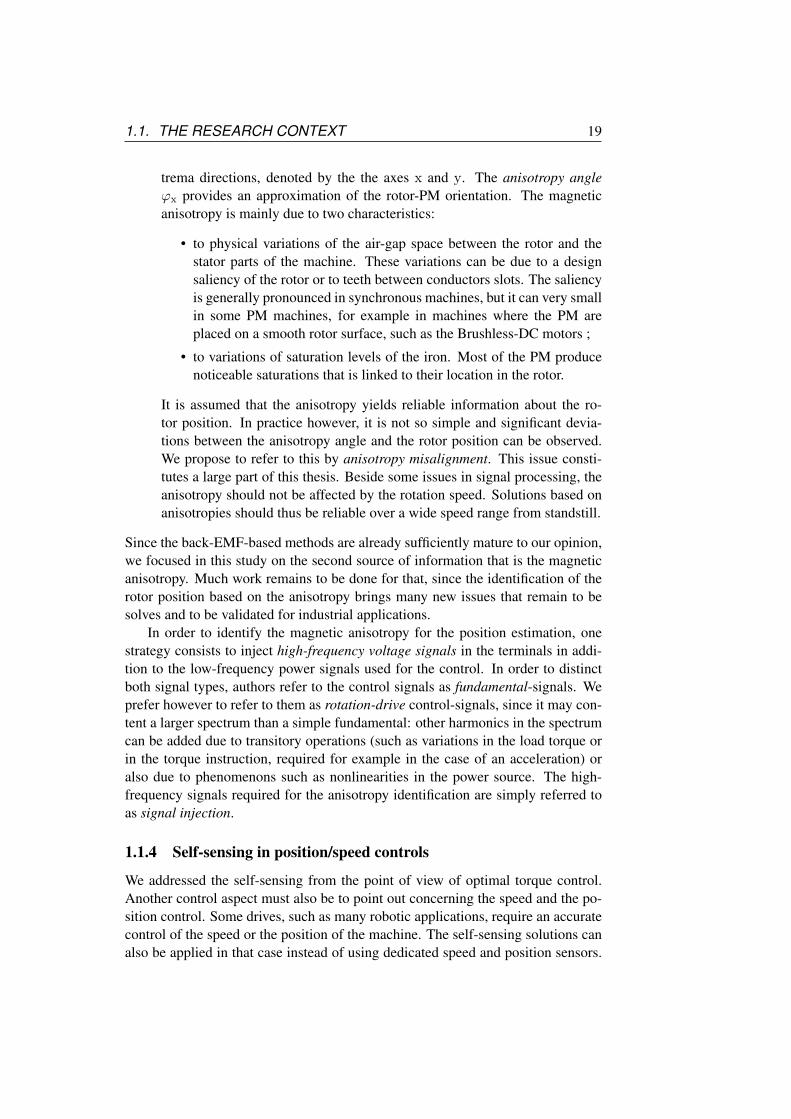
trema directions, denoted by the the axes x and y. The anisotropy angleϕx provides an approximation of the rotor-PM orientation. The magneticanisotropy is mainly due to two characteristics:
• to physical variations of the air-gap space between the rotor and thestator parts of the machine. These variations can be due to a designsaliency of the rotor or to teeth between conductors slots. The saliencyis generally pronounced in synchronous machines, but it can very smallin some PM machines, for example in machines where the PM areplaced on a smooth rotor surface, such as the Brushless-DC motors ;
• to variations of saturation levels of the iron. Most of the PM producenoticeable saturations that is linked to their location in the rotor.
It is assumed that the anisotropy yields reliable information about the ro-tor position. In practice however, it is not so simple and significant devia-tions between the anisotropy angle and the rotor position can be observed.We propose to refer to this by anisotropy misalignment. This issue consti-tutes a large part of this thesis. Beside some issues in signal processing, theanisotropy should not be affected by the rotation speed. Solutions based onanisotropies should thus be reliable over a wide speed range from standstill.
Since the back-EMF-based methods are already sufficiently mature to our opinion,we focused in this study on the second source of information that is the magneticanisotropy. Much work remains to be done for that, since the identification of therotor position based on the anisotropy brings many new issues that remain to besolves and to be validated for industrial applications.
In order to identify the magnetic anisotropy for the position estimation, onestrategy consists to inject high-frequency voltage signals in the terminals in addi-tion to the low-frequency power signals used for the control. In order to distinctboth signal types, authors refer to the control signals as fundamental-signals. Weprefer however to refer to them as rotation-drive control-signals, since it may con-tent a larger spectrum than a simple fundamental: other harmonics in the spectrumcan be added due to transitory operations (such as variations in the load torque orin the torque instruction, required for example in the case of an acceleration) oralso due to phenomenons such as nonlinearities in the power source. The high-frequency signals required for the anisotropy identification are simply referred toas signal injection.
1.1.4 Self-sensing in position/speed controls
We addressed the self-sensing from the point of view of optimal torque control.Another control aspect must also be to point out concerning the speed and the po-sition control. Some drives, such as many robotic applications, require an accuratecontrol of the speed or the position of the machine. The self-sensing solutions canalso be applied in that case instead of using dedicated speed and position sensors.

20 CHAPTER 1. INTRODUCTION
The position estimation is therefore not only used to compute the optimal torque,but it is used in feed-back loops controlling speeds and positions. The speed isgenerally obtained from an observer using, in input, the estimated rotor position.The observer can eventually include dynamic models of the machine in order toimprove the speed estimation. This benefit of the self-sensing is valid for anytype of machine [5], that can be PM machines, but also induction machines andDC-motors [8]. The solution to track the rotor position in case of induction ma-chines and DC-motors are however limited to small magnetic anisotropies mainlyrelated to rotor teeth. The small amplitude and the high-harmonic content of theanisotropies in these cases bring some further issues that are not met in PM ma-chines. Some references focus on these questions and are mentioned in this thesis,but it is not further addressed.
Let us highlight here a third source of rotor-position information specific todouble-fed asynchronous machines: thanks to their double circuits, one at the ro-tor and the other at the stator, the relative shift between these circuits provide anadditional source of information, used by [9]. This source exists in any machinewith connection to the rotor and can certainly be used in synchronous machine withwound rotor, but we did not find references about this. Note that these machinesare generally less robust because of the slip rings required for the rotor connection.Other types of connections using the coupling of two machines also exist, but thesesolutions greatly deviate from the studied applications of the PM machines.
1.2 Technical Overview
1.2.1 Main issues and contributions
As introduced previously, this Ph.D. thesis summarizes a research work focus-ing on the anisotropy-based self-sensing methods using high-frequency signal-injections without additional sensors. Different types of signals were implemented,such as the so-called test pulses, rotating and pulsating signals, at different fre-quencies. All these types of signals have their advantages and their drawbacks,depending on the application.
The progress of the work was closely related to the issues faced during the im-plementation of the methods on a challenging experimental Brushless DC (BLDC)motor, that is a specific type of PM machine described in the next subsection.Among the issues, we have the significant misalignment between the rotor positionand the anisotropy, whose orientation is identified by the high-frequency signals.This is firstly due to significant load currents in the stator that leads to an error shiftwith respect to the real position of the rotor, but also to space harmonics in the mag-netic field and in the stator winding distribution leading to an oscillating error in theposition estimation. This last error is illustrated in Figure 1.3 by the anisotropy an-gle ϕx as a function of the rotor position located by its quadratic angle ϕq. Thesemisalignments can be neglected in certain machine designs, but they are highlypronounced in the the experimental BLDC motor. They can significantly affect the

1.2. TECHNICAL OVERVIEW 21
−90
−60
−30
0
30
60
90ϕ
x
0 60 120 180 240 300 360 ϕq
Figure 1.3: Results with the experimental BLDC motor: anisotropy angle ϕx estimatedusing signal-injection, as a function of the PM-rotor orientation, related to ϕq.
optimal torque control, reducing its efficiency. They should therefore be assed andcompensated. Many publications analyze the misalignment through finite-elementsimulations and address approximate technical solutions. But the theory of thismisalignment is not greatly beloved by the community of researchers. To bridgethis gap, we largely studied the possibility to develop a simple analytical modelthat could given instructive information about the phenomenon of the anisotropy.This development was rather long, providing very interesting models to be used.But it did unfortunately not leave much time to concretely implement a solution.Possible solutions are however suggested in this thesis.
phas
ea
outp
ut
IGBT diode
PWM
sign
als
dc-b
us
+ high level
− low level
phas
eb
outp
ut
phas
ec
outp
ut
Figure 1.4: Design of the two-level three-phase VSI
Another important issue is due to nonlinearities in the voltage supplied by thevoltage-source inverter, corresponding to deviations between the expected voltageand the real output voltage. The topology of the two-level three-phase voltagesource inverter (VSI) used in the experiments is shown in Figure 1.4. This type ofinverter operates by switching each phase output between a high-level voltage anda low-level voltage from the dc-bus input, commanded by pulsewidth modulated(PWM) signals. The self-sensing methods require an accurate knowledge of thesupplied voltage. For cost and reliability reasons however, the voltage is often notdirectly measured. In that case, self-sensing operations rely on the command volt-age sent to the ship generating the PWM. The behavior of the VSI is however not
22 CHAPTER 1. INTRODUCTION
t
t
PWM cycle
dc-b
usvo
ltage
PWM phase voltage
phase current ripples
Figure 1.5: PWM voltage signal and the current ripples
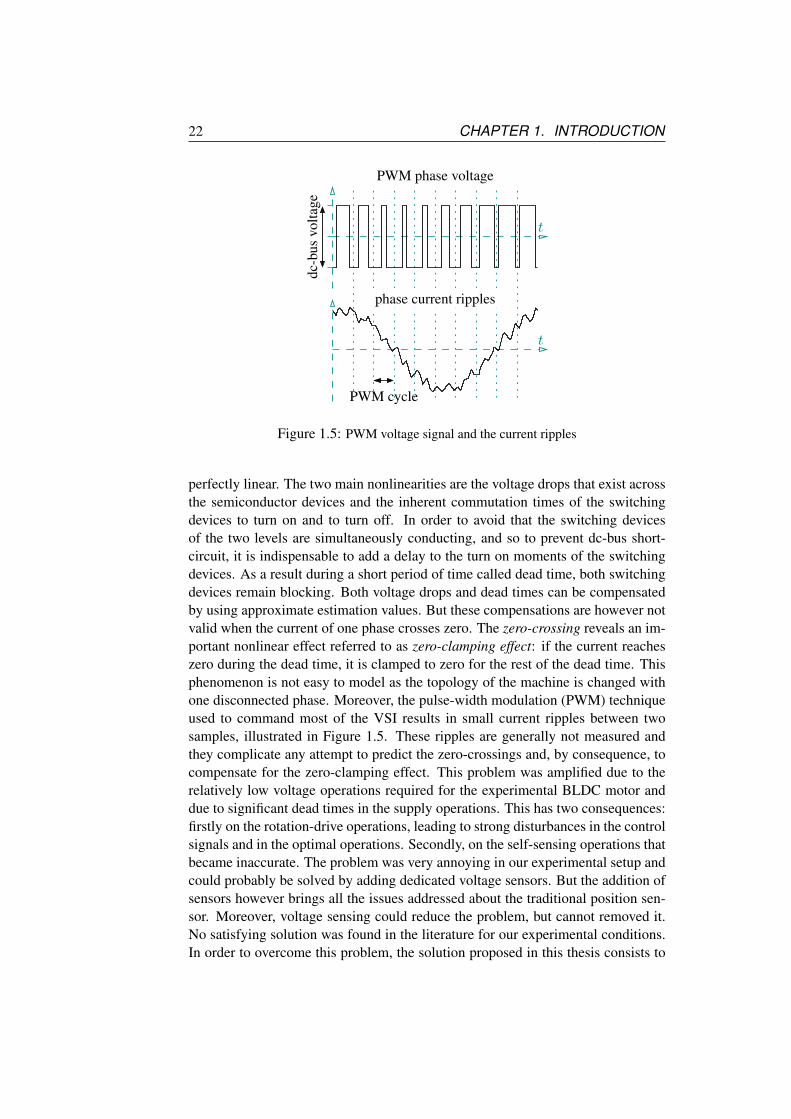
perfectly linear. The two main nonlinearities are the voltage drops that exist acrossthe semiconductor devices and the inherent commutation times of the switchingdevices to turn on and to turn off. In order to avoid that the switching devicesof the two levels are simultaneously conducting, and so to prevent dc-bus short-circuit, it is indispensable to add a delay to the turn on moments of the switchingdevices. As a result during a short period of time called dead time, both switchingdevices remain blocking. Both voltage drops and dead times can be compensatedby using approximate estimation values. But these compensations are however notvalid when the current of one phase crosses zero. The zero-crossing reveals an im-portant nonlinear effect referred to as zero-clamping effect: if the current reacheszero during the dead time, it is clamped to zero for the rest of the dead time. Thisphenomenon is not easy to model as the topology of the machine is changed withone disconnected phase. Moreover, the pulse-width modulation (PWM) techniqueused to command most of the VSI results in small current ripples between twosamples, illustrated in Figure 1.5. These ripples are generally not measured andthey complicate any attempt to predict the zero-crossings and, by consequence, tocompensate for the zero-clamping effect. This problem was amplified due to therelatively low voltage operations required for the experimental BLDC motor anddue to significant dead times in the supply operations. This has two consequences:firstly on the rotation-drive operations, leading to strong disturbances in the controlsignals and in the optimal operations. Secondly, on the self-sensing operations thatbecame inaccurate. The problem was very annoying in our experimental setup andcould probably be solved by adding dedicated voltage sensors. But the addition ofsensors however brings all the issues addressed about the traditional position sen-sor. Moreover, voltage sensing could reduce the problem, but cannot removed it.No satisfying solution was found in the literature for our experimental conditions.In order to overcome this problem, the solution proposed in this thesis consists to

1.2. TECHNICAL OVERVIEW 23
estimate the amplitude of the current ripples and to add an offset in the currentreference in order to maintain the current ripples far enough from zero. This offsetis selected in order to minimize its impact on the torque and the performances ofthe machine.
Another issue comes from the impact of the resistor and the eddy currents inthe identification operations. They are generally neglected in self-sensing opera-tions using high-frequency signals, assuming a purely inductive behaviour of themachine circuit. In practice however, they can lead to estimation errors. This topicis addressed in some publications, but we propose a further analysis based on adiscrete-time model that we develop in this thesis. The issue of the resistance canbe combined with a last issue related to the separation between the signals for theself-sensing operations and the rotation-drive operations. It is shown that these is-sues are significantly reduced using the highest possible frequency for the signalinjection, that is one third of the sampling frequency (for rotating signals) or halfthe sampling frequency (for pulsating signals) used for the digital operations. Weproposed a very simple and very reliable solution based on discrete-time opera-tions and FIR filters. The efficiency and the robustness are verified in the driveof the experimental BLDC motor, including all the problems due to the low sen-sor resolution, due to anisotropy misalignment and due to the nonlinearities of thevoltage-source inverter. This is the most relevant contribution of this work.
1.2.2 Experimental bench
Figure 1.6: Experimental BLDC motor.
The experiments are performed on a 3 kW three-phase in-wheel motor brushless-DC (BLDC) motor with P = 14 pairs of surface-mounted permanent-magnets inan outer rotor, presented in Figure 1.6. It was developed by the company Tech-nicrea, France, for the propulsion of small vehicles and initially intended for theproject Velapac of the company SERA (Societe d’Etude et de Recherche Automo-bile). This is a 14 inch diameter cylindrically shaped motor and it weighs 13.5 kg.The yoke is made of sheet of FeSi (type Ugine 250-35HA) and the PM are made of
24 CHAPTER 1. INTRODUCTION
Nd-Fe-B, producing peak magnetic fields of 0.66 T in the air-gap. It is cooled byforced air convection. The rated torque is 150 Nm from standstill to 191 rpm, cor-responding to a rated stator current of 134 A. The maximum torque decreases downto 57.3 Nm, corresponding to a rated stator current of 55 A, when the rated rotationspeed is of 500 rpm is reached, corresponding to a rotation electrical-frequency of14× 500/60 = 116 Hz. The motor performance is 91 % at 500 rpm.
The motor is fed with an IGBT voltage-source inverter (VSI) from SEMIKRON(model SKM 50GB123D with a rated current of 50 A), which is supplied by a DC-bus voltage set around vdc = 50 V. Owing to the relatively small inductance ofthe motor, the manufacturer Technicrea recommends not exceed a DC voltage ofvdc < 72 V. This voltage is supplied by a thyristor power rectifier from ACEC(model REDACEC S, that is initially a power driver for DC-motor). The pulse-width modulated (PWM) signals commanding the IGBT of the VSI are generatedby a DSP controller unit from Texas Instruments (model TMS320F240DSP) set ina dSpace card (model DSP103 PPC Controller Board).
The same dSpace card is used to measure the phase currents at the machineterminals, the DC-link voltage of the power rectifier and to perform the digitalcontrol operations. The maximum sampling frequency for the current measure-ments is νs = 13 kHz (obtained experimentally). This frequency is mainly limitedby the time required to perform the computations, that must be lower than the sam-pling period Ts = 1/νs minus all the delays of the input/output operations. Theself-sensing control method has been implemented using partly Simulink codes(Matlab R13 with Simulink 5.0.2) and mainly C codes, compiled and loaded in thecard (Real-Time Workshop 5.0.1).
The BLDC motor is equipped by hall-effect sensors from Honeywell (400SSSeries), but they are not used in this study. The position estimated by the self-sensing operations are compared to the position given by a 8192-pulses incrementalencoder from Sick|Stegmann (model DRS61-A4A08192).
1.2.3 Flow chart of the self-sensing control
The anisotropy angle ϕx can be estimated by the injection of high-frequency sig-nals in addition to the low-frequency voltage computed by the normal rotation-drive operations. The resulting high and low-frequency contents of the currentresponse are filtered for self-sensing and rotation-drive operations.
Figure 1.7 gives an overview of the self-sensing control operations using signal-injections in flow chart, including the different issues addressed in this work. Start-ing from the upper left part of the flowchart:
• The speed controller computes a current-amplitude instruction i??c from theerror between the user speed-instruction ω?c and the estimated PM rotationspeed ωq ;
• The current instruction is oriented following the estimated angle ϕq, corre-sponding to the torque-producing orientation related to the rotor-PM posi-

1.2. TECHNICAL OVERVIEW 25
Con
trol
ler
Cur
rent
Con
trol
ler
Spee
dZ
ero-
Cro
s.Pr
even
tion
Ang
le/S
peed
Obs
erve
rFi
lters
Inve
rter
Non
linea
ritie
sC
ompe
nsat
ion
Self
-Sen
sing
Est
imat
or
Pow
erIn
vert
erD
river
Mv?
i??
cω? c
i??
ci? c
Inve
rter
ωq
v? c
i c
∠ ϕq
v? i
i c i iω
q
vdc
DC
-bus
i
Pow
ersi
deC
ontr
olsi
de ϕx
Figure 1.7: Global flow chart presenting the main blocs of the self-sensing control usingsignal-injections.

26 CHAPTER 1. INTRODUCTION
tion ;
• A zero-crossing prevention block computes a new current instruction i?c byadding an offset in order to prevent the zero-crossing nonlinearity of thepower inverter ;
• The current controller computes the voltage command v?c from the error be-tween the current instruction and the filtered current input ic ;
• A high-frequency voltage v?i is added to v?c , and the total voltage commandv? is sent to the block driving the power inverter ;
• If the voltage applied to the machine is not measured, the inverter nonlineari-ties should be compensated in order to improve the correspondence betweenthe command voltage and the output voltage from the inverter ;
• The additional high-frequency voltage v?i produces a high-frequency currentvariation ii in addition to the low-frequency current ic used for the rotationcontrol. Both are separated by applying low-pass and high-pass filters ;
• The high-frequency current ii is used to compute the estimation of the anisotropyangle ϕx ;
• An observer is used to provide an estimation of the rotor-PM speed ωq and afiltered estimation of the angle ϕq, possibly taking the misalignment of theanisotropy into account.
1.3 Thesis Plan
This thesis is organized in four chapters, described hereafter. This organizationdoes not correspond to the steps of the work progress, but to the sequence of con-cepts successively required to understand the issues met in the self-sensing imple-mentation.
Chapter 2, entitled “Electromagnetic Model”, addresses the modelling of theelectromagnetic phenomena in the case of cylindrical machines with nonlinearmagnetic characteristics. Relations between the magnetic flux linked by one phasecoil and the different magnetic contributions, that are the stator current and the per-manent magnets for the PM machine, are developped. Special attention is given tolinearized relations around working points, leading to the definition of incrementalrelations. These relations are extended to polyphase machines using the concept ofspace vectors to represent the phase values. This leads to the concept of anisotropy,represented by the anisotropic incremental self-inductance factor between the smallcurrent and their contribution to the linked flux. The relations are further simplifiedfor the case of a three-phase machine without neutral connection. The incrementalself-inductance therefore takes the form used in self-sensing operations. Throughthis chapter, we want to reintroduce the concept of space vectors and to illustrate

1.3. THESIS PLAN 27
their potential for any number of phases. We want also to show the origin of theanisotropy, that is the basis of the considered self-sensing strategy. This allowsto understand the causes of the anisotropy misalignment and to assess them in thecase of the experimental BLDC motor.
Chapter 3, entitled “Electrical Circuit Model”, addresses the modelling of therelation between the currents and voltages at the machine terminals, firstly neglect-ing the eddy currents and secondly including them. Since the operations are per-formed by digital computation devices, the initial continuous-time model is sub-stituted to a discrete-time model. Special attention is given to parameter distor-tions due to the discretization and due to the pulsewidth modulation of the voltagesource, in particular for the case including eddy currents. The signal-injectionmethods mainly identify an impedance (or inversely an admittance, depending onthe point of view), that can be modelled in equivalent apparent inductive and resis-tive effects. The theoretical variations of these apparent parameters as a functionof the signal frequency are compared to measurements performed on the experi-mental BLDC motor, in order to validate the models. This chapter does not presentany issue nor solution required for the self-sensing, but highlight the phenomenonof apparent parameter variations, that are experimentally observed. Through thischapter, we want to show that the discretization of the model in case of large eddycurrents is not an obvious operation, and that its validity is not guaranteed. Wepropose therefore a tool allowing to assess the validity from the knowledge of thecontinuous-time model parameters.
Chapter 4, entitled “Voltage-Source Inverter”, addresses the working of theconventional two-level three-phase voltage-source inverter (VSI) based on IGBTcommanded by conventional pulsewidth-modulated (PWM) signals with a fixedfrequency. This is not the only type of power inverter nor the only type of commandsignals, but it is a proven and widespread industrial solution until now. Moreover, itis used in the experimental drive. The different nonlinearity issues met in that typeof PWM-VSI are introduced. The most problematic is referred to as zero-clampingeffect and occurs when a phase current crosses zero. By consequence, two meth-ods to prevent zero-crossings are proposed and implemented for the experimentaldrive. Note that the presented issues are strongly related to the PWM-VSI type.They could possibly be removed using newer VSI types, or by the possible futuremanufactures of new and more efficient semiconductors.
Chapter 5, entitled “Signal Processing”, addresses firstly an overview of thevector controls and of different self-sensing methods. The case of the high-frequencysignal-injected is secondly addressed in details. Concrete self-sensing operationsare introduced depending on the type of injected signal. Different issues are ad-dressed: the problem of the measurements noise, the separation between self-sensing and rotation-drive operations, the impact of the resistance, the sources ofdisturbances, the computation requirements, the robustness and the settling times.All these issues are analyzed regarding the case of the experimental drive for dif-ferent types of signals (rotating, pulsating and alternating) at different frequencies.Through this chapter, we firstly want to justify the choice of the signal injection for

28 CHAPTER 1. INTRODUCTION
the experimental case. It is however not the only solution and we propose compari-son tables, since others solutions could be more advised for other drive conditions.The quality of the position estimation is illustrated by experimental results.

Chapter 2
Electromagnetic Model
This chapter addresses the electromagnetic model of the permanent-magnet (PM)machine. This model describes the relation that exist between the different mag-netic sources in the machine and the magnetic flux linked by the stator coils, namedphases. In a permanent-magnet (PM) machine, the magnetic sources are the PMmounted in the rotor and the currents flowing in the stator coils. This relationmay present nonlinear and anisotropic properties, that are defined in this chap-ter. The electrical torque due to the interaction between the magnetic field andthe currents flowing in the coils is also introduced. This model provides essentialmathematic tools to understand the behaviour of the machine in order to introducecontrol schemes and self-sensing methods in the last chapter.
2.1 Introduction
The concept of space vectors is widely used in machine control to describe therelations between the electromagnetic values [10, 11, 12, 13, 1]. This concept isalso referred to as two-dimensional equivalent values or space phasors in somepublications. It provides a significant simplification tool for the relations, espe-cially for three-phase machines. This concept was initially addressed with the ap-proximation of fundamental magnetomotive-force distributions by R. H. Park in1929 [14, 15, 16, 17], and assuming synchronous operations, i.e. sinusoidal vari-ations of the power signals. The first approximation is equivalent to assume thatthe magnetic field and the conductor distributions in the stator can be modelled byfundamental sinusoidal functions on the pole-pairs, as described by J. Holtz [18].
Many authors continue to maintain this approximation, even for recent vari-able speed drives and for machines where it could not be valid. In the early 20thcentury, this choice was only dictated by limitations of the analog control devicesused at this time, and not to mathematical restrictions. The concept provides in factvery interesting relations also for machines presenting significant harmonics. Themodelling in that case can be initiated by Fourier series developments of the differ-ent design characteristics and the different electromagnetic phenomenon occurring
29

30 CHAPTER 2. ELECTROMAGNETIC MODEL
all around the space separating the stator and the rotor, called the air-gap. Theseseries provide results that can be easily related to the concept of space vectors, thatis extended for the occasion. In a similar way, this methodology was proposed byG. Maggetto [19] in 1973 and by H. R. Fudeh [20, 21, 22] in 1983, in order toestimate the oscillations in the torque during synchronous operations. The consid-eration of the harmonics is of first important in some machines designs, such asin concentrated windings topologies or in recent brushless DC motors. They cansignificantly affect the behaviour of the machine and results in oscillating errors inthe position estimated by self-sensing methods. This is addressed in this chapter.
Another widespread simplification in the machine modelling consist to ne-glect the nonlinear magnetic characteristics linking the magnetic sources to theproduced magnetic B-field, and corresponding to magnetic saturations in the iron.This choice is only justified by the strong complexity to find simple models ofthe saturation. These nonlinear magnetic characteristics are however an importantcontribution to the anisotropic properties of the machines, that are expected forcertain self-sensing methods. It can moreover be the only source of anisotropy inthe case of surface-mounted PM. Many authors dealing with anisotropy-based self-sensing methods must assume the magnetic nonlinearities, but simplifies the modelassuming that the magnetic state of the machine is mainly function of the PM field,neglecting the contribution of the stator currents. This contribution may howeveraffect the magnetic state and result in a shift of the anisotropy orientation used toestimate the rotor position, as discussed in [23] with a model based on magneticco-energy. This is also addressed in this chapter.
In the vast number of recent publications, the space vectors description areoften very short using variable formalisms, and restricted to the fundamental modelapproximation. In this chapter, we propose therefore to clarify the descriptionof the concept in a simple formalism. In a first time, the concept is generalizedfor an arbitrary n number of phases and taking the harmonics into account. It isreduced to three-phase machines only in a second time, leading to a more intuitiveexpression of the anisotropy. This anisotropy yields an orientation that can be usedto estimate the rotor position. This orientation is affected by the two mentionedsubjects: harmonics, leading to anisotropy oscillations, and nonlinearities, leadingto anisotropy shifts. For convenience, both effects are referred to as anisotropymisalignments in this document.
∼
This chapter is organized as follows: the section 2.2 introduces elementarydescriptions of the design and the topologies of different electric machines, in-cluding the brushless DC (BLDC) motor ; Section 2.3 introduces some importantassumptions for the modelling and describes several relations from the point ofview of the stator coils, referred to as stator phases. Among them, we have therelation between the magnetic field and the magnetic flux linked by one coil, thenonlinear relation between the magnetomotive forces and the magnetic field, the

2.2. ELECTRIC MACHINE DESIGNS 31
axisrotation
air−gap
front−edge
back−edge
stator/rotor
core
rotor/stator
yoke
Figure 2.1: Illustration of a rotating electrical machine with cylindrical shaped parts.
corresponding incremental relation useful for anisotropy-based self-sensing the-ory, and the expression of the electrical torque ; Section 2.4 introduces the conceptof space vectors for polyphase machines, assuming any number of phases and in-cluding harmonic aspects. The relations previously described are transposed inrelations between the space vectors ; Section 2.5 specifically develops the relationsfor the widespread case of three-phase machines and introduces the mathematicalexpression of the anisotropic relation, as further used in this thesis ; Section 2.6 ap-plies the modelling to the experimental BLDC motor and adjusts its characteristicsby comparing experimental results to simulation results. This allows some drawsome conclusions about the impact of harmonics and stator currents in anisotropymisalignment ; A summary of the important elements of this chapter is given insection 2.7.
2.2 Electric Machine Designs
As illustrated in Figure 2.1, a rotating electrical machine is made of two iron partsrotating with respect to each other. By convention, one part is called the statorand the other part is called the rotor. The stator is generally the part mounted onthe same pedestal as the power electronic driving the machine. The space thatseparates the rotor and stator parts is called the air-gap. Most of the electricalmachines present an inner-rotor design: the rotor is the core of the machine andis accessible through a rotation axis, while the stator is the yoke surrounding thecore. The reverse outer-rotor design, with the rotor surrounding the stator, is lesscommon. This is the design of our experimental in-wheel motor, intended forsmall car traction, where the rotation is assumed to be transmitted by a tire directlymounted on the rotor external surface, while the stator replaces the wheel rim andis fixed to the chassis of the car.
Most of the machines are formed by the assembly of cylindrical shaped parts.

32 CHAPTER 2. ELECTROMAGNETIC MODEL
cross
−se
ctio
n
coilmagnetic−field
Four pole−pairs machine
Equivalent single−pole−pair
one pole−pair
terminals
North
South
θ = PΘ
⇒
θ = 0
θ = 2π
θ = 0θ = 2π
Figure 2.2: Illustration of a machine cross-section considering only one coil in the statorcore (outer-rotor design), and the equivalent single-pole-pair representation. In a cross-section, denotes a current flowing from back to front-edge and ⊗ denotes an inverseflow.
In other words, the cross-section of the machine is the same at any axial positionbetween front and back edges. This is the case of our experimental motor. In such adesign, the conductors are laid in parallel to the rotation axis, in slots that are gener-ally close to the air-gap surface, as illustrated in Figure 2.2 with one coil. Machinesgenerally contain several interlaced coils, referred to as phases. And, it is assumedthat the magnetic field crosses radially the air-gap and has no axial component. Inless conventional designs (not illustrated), the magnetic field crosses axially themachine through disks. They are referred to as axial-flux machines. These lessconventional designs are not specifically studied in this document, but most of theproposed theory could however be adapted and applied to them.
As illustrated in Figure 2.2, an electrical machine is often made by the jux-taposition of identical structure patterns along the physical angular position Θ ∈0, 2π, where identical electromagnetic phenomenons are repeated. Such a pat-tern is referred to as pole-pair substructure since the magnetic field loops in that

2.2. ELECTRIC MACHINE DESIGNS 33
place between two locations called North and South poles, crossing the air-gap.Thanks to the repetition property, the model of a multipole machine can be re-stricted to an equivalent single-pole-pair representation along an electrical angularposition θ ∈ 0, 2π. If P is the number of pole-pairs the relation is: θ = PΘ.This property is however lost if the rotor and stator axes are misaligned (develop-ments assuming misalignment are found in [24]), if small variations occur betweensubstructures (such as differences in the aging of permanent magnets for instance)or if the machine is immersed in a significant external magnetic field. These specialsituations are not studied in this document and we assume therefore identical pole-pairs. Note some interesting designs where the number of identical structures arenot the same at the stator and at the rotor. This is the case of the modular topolo-gies of some BLDC motors as proposed by [25]. In that case, P is the commondenominator between the stator and the rotor structures.
We distinct two main types of machines depending on the supply strategies atthe stator side: the so-called DC and AC machines. An AC machine is a polyphasemachine generally made of minimum three stator coils, whose windings are dis-tributed over the circumference of the stator, and presenting at least one connectibleoutput terminal. In so-called star-connection topologies, the others terminals ofthe coils can be connected in one point, often called the neutral point. In so-calleddelta-connection topologies, the terminals are connected by peers. The variationsof the currents in the coils are either due to the alternating character of the supply-ing voltages, or they are controlled electronically by the modulation of an externalDC-bus voltage. The torque in electrical machine is produced by the electromag-netic interactions between the stator and the rotor. The main part of the torque isdue to the interaction of the stator current with the magnetic field produced fromthe rotor. This is produced either by the magnetic reaction in a closed coil locatedin the rotor (defining the induction machines, also called asynchronous machines),by a fixed current flow (DC) in one rotor coil (defining the synchronous machines)or by currents in polyphase rotor-coils (defining the double-fed asynchronous ma-chines). The current flow in the rotor coils can be replaced by permanent-magnets(PM), leading to the so-called PM synchronous machines (PMSM). Variations ofthe reluctance in the machine, mainly due to salient pole designs at the rotor, alsoproduce a torque (defining the reluctance motors). Only a small part of all the ACmachines types are mentioned here. A larger overview is found in [26, 27, 2].
A DC machine is generally made of a multitude of windings distributed overthe circumference of the rotor. The current flow in the different windings is com-mutated mechanically by brushes rubbing on rings, while the global value of thecurrent flowing through two accessible terminals is controlled externally. In com-parison to the AC machines, the drive of the DC machines is much simpler, butthis type of machine is generally more expensive and requires a higher mainte-nance due to mechanical frictions. Note that the electric circuits of DC machinescan be modeled assuming an equivalent high number of phases. This is made by[28]. The magnetic field from the stator can be produced by a fixed current flow(DC) in one coil or by permanent-magnets (PM). Note that some machines hold
34 CHAPTER 2. ELECTROMAGNETIC MODEL
additional compensation circuits for armature reactions and damping circuits, thatare not discussed here.
The Brushless-DC (BLDC) machine reproduces the principle of the DC ma-chine with PM, where the rotor and the stator topologies are inverted (the PMare in the rotor). The mechanical brushes are removed and replaced by electroniccommutations. The design of the BLDC machine is however closer to an AC ma-chine than a DC machine, and can be classified among the PM machines (nonsynchronous). In order to reproduce a behaviour similar to a DC machine, theconductors of each phases are generally concentrated in low number of slots. Thereluctance variations due to the teeth separating the slots and the interaction withthe PM may produce significant cogging torque. This effect have an important im-pact on the quality of the drive [29]. This is the case in the experimental BLDCmotor of this study. The designs can be improved in order to reduce the coggingtorque, such as the modular topology described in [25] or using skewing of thestator conductors [29].
As explained in the introduction, the PM machines have generally strong ad-vantages compared to other types: they present high power densities (power withrespect to the size and the weight), robustness and reliability. Their price is mainlyrelated to the rare magnetic material cost, that decreased during last decades. Byconsequence, this work mainly focuses on that type of machine. To our opinion, itis however important to develop models and strategies that could be possibly ap-plied to other machines types. This is not specifically mentioned in this work, butonly small adaptations should be required to transpose the model to other designs.
2.3 Electromagnetic Relations
In this section, we develop the analytical relation between the magnetic flux ψplinked by the coil of one phase, numbered p, with the different magnetic contri-butions. In a permanent-magnet (PM) machine and neglecting the eddy currents,these contributions are the currents ip′ flowing in the stator coils of the differ-ent phases p′, multiplied by stator inductance parameters lpp′ , and the permanent-magnets on the rotor written ψPM,p. Due to strong nonlinear properties of themagnetic materials, the relation between the flux variations dψp and small currentvariations dip′ can be strongly dependent on the magnetic state of the machine.Local linearized values of the inductances lt,pp′ , denoted by the lower index t, aretherefore required. They are called incremental inductances or tangential induc-tances [30, 31]. For convenience all the values and the relations related to smallvariations are called incremental in this work. The expression of the torque due tothe interaction between the stator currents and the magnetic field is also introducedin this section.
2.3. ELECTROMAGNETIC RELATIONS 35
~1r
R
~B
S
V
lm
~1z
~1Θ
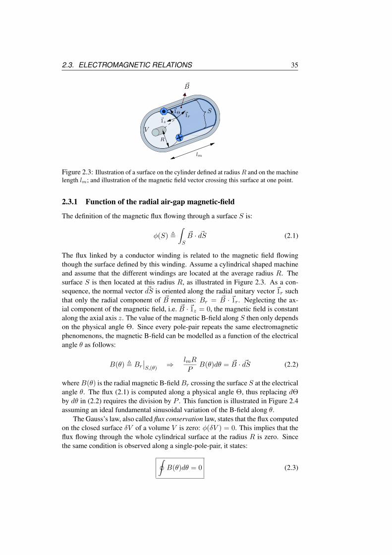
Figure 2.3: Illustration of a surface on the cylinder defined at radiusR and on the machinelength lm; and illustration of the magnetic field vector crossing this surface at one point.
2.3.1 Function of the radial air-gap magnetic-field
The definition of the magnetic flux flowing through a surface S is:
φ(S) ,∫S
~B · ~dS (2.1)
The flux linked by a conductor winding is related to the magnetic field flowingthough the surface defined by this winding. Assume a cylindrical shaped machineand assume that the different windings are located at the average radius R. Thesurface S is then located at this radius R, as illustrated in Figure 2.3. As a con-sequence, the normal vector ~dS is oriented along the radial unitary vector ~1r suchthat only the radial component of ~B remains: Br = ~B · ~1r. Neglecting the ax-ial component of the magnetic field, i.e. ~B · ~1z = 0, the magnetic field is constantalong the axial axis z. The value of the magnetic B-field along S then only dependson the physical angle Θ. Since every pole-pair repeats the same electromagneticphenomenons, the magnetic B-field can be modelled as a function of the electricalangle θ as follows:
B(θ) , Br∣∣S,(θ)
⇒ lmR
PB(θ)dθ = ~B · ~dS (2.2)
whereB(θ) is the radial magnetic B-fieldBr crossing the surface S at the electricalangle θ. The flux (2.1) is computed along a physical angle Θ, thus replacing dΘby dθ in (2.2) requires the division by P . This function is illustrated in Figure 2.4assuming an ideal fundamental sinusoidal variation of the B-field along θ.
The Gauss’s law, also called flux conservation law, states that the flux computedon the closed surface δV of a volume V is zero: φ(δV ) = 0. This implies that theflux flowing through the whole cylindrical surface at the radius R is zero. Sincethe same condition is observed along a single-pole-pair, it states:∮
B(θ)dθ = 0 (2.3)

36 CHAPTER 2. ELECTROMAGNETIC MODEL
θ
0
B(θ)
np(θ)
B(θ)
Rnp(θ)
~1θ ~1r
ϕp
ϕp
ϕd
0 90 180 360
0
B
240 θ (deg)
0 90 180
0
np
360240 θ (deg)
Figure 2.4: Illustration of the functions describing the conductor distribution of the coil pand the magnetic B-field in the equivalent single-pole-pair cross-section.
This is the first condition of the machine model, where it is assumed that the mag-netic field has no axial component, thus no edge leakage. This assumption is madein many publications, such as [32, 33].
2.3.2 Function of the conductor distribution
The conductors of each stator coil numbered by p are approached by a distributionlocated at the mean radius R and described by the function np(θ). This is illus-trated in Figure 2.4 assuming an ideal sinusoidal distribution (this is not a realisticdistribution since the punctual location of the slots is not taken into account, butthis is enough for the illustrations). The symbols and ⊗ denote the current flowsigns in these conductors assuming a positive current flowing at the stator terminalsof the phase, i.e. ip > 0 (this is a convention). We assume that windings of eachcoil along the different P pole-pairs are connected in series, such as illustrated inFigure 2.2. In that case, np(θ) is defined as the number of conductors at everylocation θ along one single-pole-pair. The case where windings are connected inparallel requires some slight adaptations of the relations, adding a factor P . Thisis not done here.
In most of the machines, it can be assumed that the conductors are wound bypairs, such that the integral of np(θ) along the single-pole-pair is equal to zero:
∮np(θ)dθ = 0 ∀p (2.4)
This is the second condition of the machine model. Note that the conditions (2.4)and (2.3) are not equivalent and both required for the modelling.

2.3. ELECTROMAGNETIC RELATIONS 37
np(θ)
θ′
+1
−1
0 0
θ′
B(θ)
φ(θ′) Np(θ′)
Figure 2.5: Illustration of the unitary magnetic flux and the linking distribution in theequivalent single-pole-pair cross-section.
2.3.3 Relation between the flux linked by a coil and the magnetic field
The magnetic flux linked by a coil is defined as the sum of the contribution of themagnetic fluxes linked by all the windings composing the coil. In order to proposea mathematical development of the magnetic flux, let us firstly introduce to theunitary magnetic flux. The unitary magnetic flux is defined as the flux linked by anunitary winding. As illustrated in Figure 2.5, the unitary winding is defined by oneconductor located at a variable position θ′ paired with a virtual return conductorlocated at the origin θ = 0. This virtual conductor is not involved in the fluxlinked by the whole coil and its location is arbitrary (but fixed). This is justifiedas follows: summing the contributions of all unitary windings, thanks to (2.4), thetotal contribution of the virtual conductors on np(θ = 0) is zero. We define theunitary magnetic flux φ(θ′) as the flux linked by an unitary winding as follows:
φ(θ′) , lmR
P
∫ θ′
0B(θ)dθ (2.5)
where lm is the length of the machine, R is the radius of the winding locations.This definition is chosen such that the unitary flux is positive if the conductor ofthe unitary winding located at θ′ is counted positive. Note again that (2.5) neglectsthe axial magnetic field flowing through the machine edges. The total magneticflux ψp linked by the whole winding distribution of the coil p is then the integralof the elementary fluxes φ(θ′) multiplied by the number n(θ′) at every location θ′,multiplied by the pole-pair number P :
ψp , P
∮np(θ
′)φ(θ′)dθ′ (2.6)
Replacing the unitary winding by its expression (2.5), (2.6) yields:
ψp = lmR
∮θ′
∫ θ′
θ=0np(θ
′)B(θ)dθdθ′ (2.7)

38 CHAPTER 2. ELECTROMAGNETIC MODEL
jPM(θ)
~dl = Rdθ~1θ
θ′
0
iron
air
iron
δo(θ)
l
jp(θ)
dS
Figure 2.6: Illustration of the slice S in the equivalent single-pole-pair cross-section,where jp(θ) if the contribution from the current flowing in the phase p and jPM(θ) is theequivalent contribution from the permanent-magnets to the current density j(θ).
Inverting the successive order of integration yields:
ψp = lmR
∮θ
(−∫ θ
θ′=0np(θ
′)dθ′)B(θ)dθ (2.8)
This expression can be shorten if we introduce the linking distribution Np(θ) asthe following integral of the distribution np(θ′) between θ′ = 0 and θ:
Np(θ)−Np(0) , −∫ θ
0np(θ
′)dθ′ (2.9)
As illustrated in Figure 2.5. This distribution is defined within an arbitrary constantNp(0), but due to the property (2.3), this constant is removed in (2.8) and it yields:
ψp = lmR
∮Np(θ)B(θ)dθ (2.10)
We obtain here a quite simple expression linking the magnetic flux to the mag-netic field multiplied by the linking distribution and integrated on a single-pole-pairrevolution.
2.3.4 Relation between the magnetic field and the magnetomotive forces
The integral form of the Ampere’s circuital law states that:∮l
~H · ~dl =
∫S
~j · ~dS (2.11)
where l is the contour of an arbitrary surface S, ~j is the vector of the currentdensity and ~H is the vector of the magnetic H-field. These vectors should not beconfused with the space vectors that are further used in this chapter. As illustrated

2.3. ELECTROMAGNETIC RELATIONS 39
in Figure 2.6, we define the surface S in a slice between the angle θ = 0 andθ′. Since the currents in the machine flow perpendicularly to the surface S andassuming that j(θ) models the current density included in an elementary slice dθ,it yields:
~j · ~dS = j(θ)dθ (2.12)
We introduce the magnetomotive force distribution F (θ′), defined in this workfrom the right member integral of the Ampere’s law (2.11) computed on the sliceS:
F (θ′)− F (0) , −∫ θ′
0j(θ)dθ (2.13)
It is defined within an arbitrary constant.Note that this definition of the magnetomotive force is not conventional: it is
generally defined from the left member of the Ampere’s law (2.11), i.e. as theintegral of ~H [19, 27]. This definition is however not convenient in our develop-ments, justifying this small adaptation. For information, this value is called currentdensity distribution by [34].
The left member of the Ampere’s law is developped here below firstly in thecase of an unsaturated iron (infinite permeability of the iron) and in the case of asaturated iron (local diminutions of the permeability).
Unsaturated case
The path l is partly located in the iron of the stator and the rotor, partly located inthe air, crossing radially the air-gap by two angles θ = 0 and θ = θ′. In the air,the magnetic B-field is linked to the magnetic H-field by a permeability constantµo = 4π10−7N/A2:
~B = µo ~H (2.14)
In a ferromagnetic medium, such as the iron, the magnetic H-field interacts withthe magnetic dipoles of the medium, producing an auxiliary magnetic field. It issaid that the medium is magnetized. This magnetization can be modeled using acorrection factor µr, called the relative permeability: ~B = µrµo ~H [35]. The leftmember of the Ampere’s law (2.11) can therefore be separated in two integrals,one path inside the air-gap and another path inside the iron:∮
l
~H · ~dl =
∫lair
~B
µo· ~dl +
∫liron
~B
µrµo· ~dl (2.15)
This relative permeability µr is very variable depending on the iron compositionand on the magnetic H-field intensity, but it is generally be assumed to be muchhigher than the unity: µr 1 [36]. Assuming that the value of the magnetic B-field is not much increased in the iron compared to its value in the air (thank to theflux conservation principle), the integral in the iron of (2.15) can be neglected:∮
l
~H · ~dl ≈∫lair
~B
µo· ~dl =
∫δo(0)
~B
µo· ~dl −
∫δo(θ)
~B
µo· ~dl (2.16)

40 CHAPTER 2. ELECTROMAGNETIC MODEL
where δo(θ) is the radial air-gap length at the angle θ. If the rotor presents saliencesor teeth, the air-gap length δo(θ) then varies also with the rotor position orientedby ϕd (the exact location of this angle is further discussed), and we can mention itwriting δo(θ, ϕd). Let us define B(θ) as the mean of the radial component of theB-field crossing the air-gap:
δo(θ, ϕd)B(θ) ,∫δo(θ)
~B · ~dl (2.17)
Combining these results (2.17) and (2.16) with the magnetomotive force (2.13)yields:
B(θ) =µoF (θ)
δo(θ, ϕd)(2.18)
The issue of the arbitrary constant F (0) in (2.13) can be neglected in (2.18). Thisis justified in the next page.
The impact of the stator slots transposed in an equivalent enlarge air-gap lengthδo(θ) is referred to as the slotting effect in the literature. This is largely addressedin many publications, such as [32, 33, 37, 38].
Saturated case
If a significant magnetic field is however flowing in the iron, the iron magnetizationreaches its saturation level resulting in a reduction of its relative permeability. Inthat case, we proposed in [39] to transpose the saturation in an equivalent local in-crease of the air-gap length δ1(θ, F, ϕd) as a function of the global magnetomotiveforce F , referred to as the magnetic state of the machine. Note that “global” meanshere that the value of δ1 at the position θ is related to the value of F everywhere,an not only at θ. The total length at the angle θ is then:
δ(θ, F, ϕd) , δo(θ, ϕd) + δ1(θ, F, ϕd) (2.19)
where we keep the mention to the rotor position ϕd, and it yields:
B(θ) =µoF (θ)
δ(θ, F, ϕd)(2.20)
The saturation does not occur equally everywhere in the iron. In some machines,this saturation mainly occurs around the stator teeth separating the winding slots,since these teeth concentrate the magnetic field in smaller sections, increasing lo-cally the magnetic field density [40, 41]. In that case, we assumed in [39] that thesaturation is a local phenomenon, such that it can be transposed as a local func-tion of F (θ), i.e.: δ(θ, F, ϕd) = δ(θ, F (θ), ϕd). This does however not correctlymodels saturations occurring more deeply than the winding slots in the stator ironneither saturations occurring in the rotor iron.

2.3. ELECTROMAGNETIC RELATIONS 41
Constant magnetomotive force
In order to satisfy the flux conservation law (2.3), it is required that F (θ)/δ(θ)does not have any constant component. Since F (θ) is defined within an arbitraryconstant, this condition can simply be added to its definition. Let us write F0 +F ′(θ) := F (θ), where F0 is the constant component and
∮F ′(θ)dθ = 0. It can be
shown that the flux conservation law on (2.20) yields:
F0 = −∮
F ′(θ)
δ(θ, F, ϕd)dθ
/∮1
δ(θ, F, ϕd)dθ (2.21)
More details can be found in [24]. In practice however, F0 is not required since itis removed in the computation of the flux linked by the phase windings (2.10).
Leakage factor
If the stator conductor windings are close the air-gap surface (no deep slots), if theair-gap length is small compared to the radius and if the iron is not saturating, it canbe assumed that the magnetic B-field in the air-gap is purely radial and of constantvalue crossing the air-gap path. As a consequence, the mean value of the field B(θ)is assumed equal to the field crossing radially the stator winding surfaceB(θ) [36].It is however a strong approximation that neglects the azimuthal components of themagnetic field flowing in the air-gap and flowing around the conductors, betweenthe stator teeth. These azimuthal components take part to the so-called leakagefield. This leakage field is related to the air-gap length δo, thus it is a functionof the rotor position ϕd in case of saliency, and it is a function of the saturationlevel linked to the magnetic state F . In order to take the leakage into account,some authors introduce a leakage factor κ(θ, F, ϕd) [36], whose inverse κ−1 isalso referred to as the Carter’s factor [19, 42, 37]:
B(θ) = κ(θ, F, ϕd)B(θ) (2.22)
Thus (2.20) yields:
B(θ) =µoF (θ)
κ(θ, F, ϕd)δ(θ, F, ϕd)(2.23)
A detailed development of κ in the specific case of unsaturated machine with con-stant air-gap length and sinusoidal magnetic fields (no harmonics) can be found inchapter 4.7. of [36]. Note that κ can be very different regarding the permanent-magnet contribution, whose the major part of the field crosses the air-gap, andregarding the stator current contribution, whose part of the field jumps betweenthe teeth. By definition, this factor κ models azimuthal phenomenons and cannottherefore be restricted to a local relationship occurring only at θ. Note also thatthey are other sources of leakage, due to rotor skewing effects and to the conductorloop at the edges of the machine for instance [26].

42 CHAPTER 2. ELECTROMAGNETIC MODEL
linearisation point
m(FPM)
BPM +BS
BPM
m′(FPM, FS)
FPM FPM + FS
B (T)
mt(F )
00
F (A)
Figure 2.7: Illustration of the nonlinear relation between the magnetic B-field B and themagnetomotive force F .
Final relation
For convenience, let us shorten the relation (2.23) introducing a factor m(θ, F, ϕd)as follows:
m(θ, F, ϕd) ,µo
κ(θ, F, ϕd)δ(θ, F, ϕd)
⇒ B(θ) = m(θ, F, ϕd)F (θ) (2.24)
Note that this expression is very general and gives no indication about the mod-elling of κ nor δ included in m. This modelling requires further investigationsand strongly depends on the machine design. The magnetic analysis of a surface-mounted PMSM design is proposed by [43]. It proposes a magnetic circuit modelin order to compute the optimal torque design based on a finite-element analysis.Another analysis is proposed by [44]. The case of saturation occurring mainly inthe teeth of a PM machine is modelled by [41]. It is however difficult to extracta simple model corresponding to (2.24) with these analysis. A strongly simplifiedmodel of m is further proposed for the experimental BLDC motor.
2.3.5 Contributions to the magnetomotive force
The magnetomotive force F (θ) can be developed as the sum of the different currentdensity contributions. The contribution of the permanent magnets from the rotorside can be modelled by an equivalent magnetomotive force (MMF) FPM(θ), asdone in [38, 43, 44]. This model is very convenient for surface-mounted PM, butshould be further analyzed for interior PM [6]. The contribution from the statorcoils to the magnetomotive force distribution can be modeled using the conductordistributions: jp(θ) = ipnp(θ), where ip is the current flowing at the phase terminalp. Using the embracing distributions (2.9), it yields: Fp(θ) = ipNp(θ) [27]. The
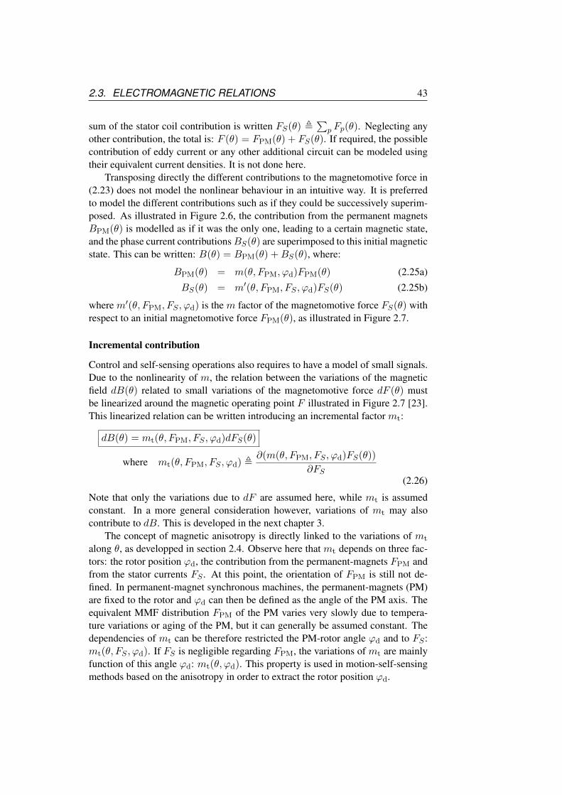
2.3. ELECTROMAGNETIC RELATIONS 43
sum of the stator coil contribution is written FS(θ) ,∑
p Fp(θ). Neglecting anyother contribution, the total is: F (θ) = FPM(θ) + FS(θ). If required, the possiblecontribution of eddy current or any other additional circuit can be modeled usingtheir equivalent current densities. It is not done here.
Transposing directly the different contributions to the magnetomotive force in(2.23) does not model the nonlinear behaviour in an intuitive way. It is preferredto model the different contributions such as if they could be successively superim-posed. As illustrated in Figure 2.6, the contribution from the permanent magnetsBPM(θ) is modelled as if it was the only one, leading to a certain magnetic state,and the phase current contributionsBS(θ) are superimposed to this initial magneticstate. This can be written: B(θ) = BPM(θ) +BS(θ), where:
BPM(θ) = m(θ, FPM, ϕd)FPM(θ) (2.25a)
BS(θ) = m′(θ, FPM, FS , ϕd)FS(θ) (2.25b)
where m′(θ, FPM, FS , ϕd) is the m factor of the magnetomotive force FS(θ) withrespect to an initial magnetomotive force FPM(θ), as illustrated in Figure 2.7.
Incremental contribution
Control and self-sensing operations also requires to have a model of small signals.Due to the nonlinearity of m, the relation between the variations of the magneticfield dB(θ) related to small variations of the magnetomotive force dF (θ) mustbe linearized around the magnetic operating point F illustrated in Figure 2.7 [23].This linearized relation can be written introducing an incremental factor mt:
dB(θ) = mt(θ, FPM, FS , ϕd)dFS(θ)
where mt(θ, FPM, FS , ϕd) ,∂(m(θ, FPM, FS , ϕd)FS(θ))
∂FS(2.26)
Note that only the variations due to dF are assumed here, while mt is assumedconstant. In a more general consideration however, variations of mt may alsocontribute to dB. This is developed in the next chapter 3.
The concept of magnetic anisotropy is directly linked to the variations of mt
along θ, as developped in section 2.4. Observe here that mt depends on three fac-tors: the rotor position ϕd, the contribution from the permanent-magnets FPM andfrom the stator currents FS . At this point, the orientation of FPM is still not de-fined. In permanent-magnet synchronous machines, the permanent-magnets (PM)are fixed to the rotor and ϕd can then be defined as the angle of the PM axis. Theequivalent MMF distribution FPM of the PM varies very slowly due to tempera-ture variations or aging of the PM, but it can generally be assumed constant. Thedependencies of mt can be therefore restricted the PM-rotor angle ϕd and to FS :mt(θ, FS , ϕd). If FS is negligible regarding FPM, the variations of mt are mainlyfunction of this angle ϕd: mt(θ, ϕd). This property is used in motion-self-sensingmethods based on the anisotropy in order to extract the rotor position ϕd.

44 CHAPTER 2. ELECTROMAGNETIC MODEL
2.3.6 Relations between the fluxes and the magnetic contributions
In practice, we generally do not have a direct access to the magnetic B-field and tothe magnetomotive force, but we have an indirect access through the linked fluxesψp = ψPM,p+ψS,p. The expression of the permanent-magnet contribution is foundcombining the expressions (2.25) and (2.24) in (2.10):
ψPM,p = lmR
∮m(θ, FPM, ϕd)Np(θ)FPM(θ)dθ (2.27)
The expression of the stator current contribution is found to be:
ψS,p =∑p′
lpp′i′p (2.28)
where lpp′ are called the stator inductances:
lpp′ , lmR
∮m′(θ, FPM, FS , ϕd) Np(θ)Np′(θ)dθ (2.29)
The expression of the incremental stator current contribution is found with (2.26):
dψS,p =∑p′
lt,pp′di′p (2.30)
where lt,pp′ are the incremental inductances:
lt,pp′ , lmRµo
∮mt(θ, FPM, FS , ϕd) Np(θ)Np′(θ)dθ (2.31)
The computation of these inductances are not directly required in self-sensingoperations, but they allow to understand how the nonlinearity properties and thedependencies of mt regarding the magnetomotive forces and the rotor positionare inherited by these incremental inductances lt,pp′ . In particular, lt,pp′ vary as afunction of the rotor position ϕd. This property is strongly expected in anisotropy-based self-sensing strategies.
2.3.7 Electrical torque
In this part, we focus on the torque produced by the interactions between the statorwindings and the magnetic B-field, called simply the electrical torque. The torquelinked to the interaction between the permanent magnets and the stator teeth iscalled the cogging torque. It is often considered as disturbing and it can be verysignificant regarding the electrical torque in some machine designs such as ourexperimental machine. It is addressed by [25] and numerically computed by finite-element method in [38]. It seems however that finding an simple analytic expres-sion of this cogging torque is rather complicated.This issue is however not studiedhere.
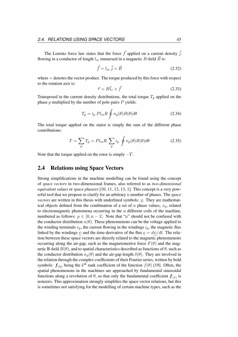
2.4. RELATIONS USING SPACE VECTORS 45
The Lorentz force law states that the force ~f applied on a current density ~jflowing in a conductor of length lm immersed in a magnetic B-field ~B is:
~f = lm ~j × ~B (2.32)
where× denotes the vector product. The torque produced by this force with respectto the rotation axis is:
~τ = R~1r × ~f (2.33)
Transposed in the current density distributions, the total torque Tp applied on thephase p multiplied by the number of pole-pairs P yields:
Tp = ip PlmR
∮np(θ)B(θ)dθ (2.34)
The total torque applied on the stator is simply the sum of the different phasecontributions:
T =∑p
Tp = PlmR∑p
ip
∮np(θ)B(θ)dθ (2.35)
Note that the torque applied on the rotor is simply −T .
2.4 Relations using Space Vectors
Strong simplifications in the machine modelling can be found using the conceptof space vectors in two-dimensional frames, also referred to as two-dimensionalequivalent values or space phasors [10, 11, 12, 13, 1]. This concept is a very pow-erful tool that we propose to clarify for an arbitrary n number of phases. The spacevectors are written in this thesis with underlined symbols: x. They are mathemat-ical objects defined from the combination of a set of n phase values, xp, relatedto electromagnetic phenomena occurring in the n different coils of the machine,numbered as follows: p ∈ [0, n − 1]. Note that “n” should not be confused withthe conductor distribution n(θ). These phenomenons can be the voltage applied tothe winding terminals vp, the current flowing in the windings ip, the magnetic fluxlinked by the windings ψ and the time-derivative of the flux e = dψ/dt. The rela-tion between these space vectors are directly related to the magnetic phenomenonsoccurring along the air-gap, such as the magnetomotive force F (θ) and the mag-netic B-fieldB(θ), and to spatial characteristics described as functions of θ, such asthe conductor distribution np(θ) and the air-gap length δ(θ). They are involved inthe relation through the complex coefficients of their Fourier series, written by boldsymbols: f (k) being the kth rank coefficient of the function f(θ) [19]. Often, thespatial phenomenons in the machines are approached by fundamental sinusoidalfunctions along a revolution of θ, so that only the fundamental coefficient f (1) isnonzero. This approximation strongly simplifies the space vector relations, but thisis sometimes not satisfying for the modelling of certain machine types, such as the

46 CHAPTER 2. ELECTROMAGNETIC MODEL
experimental BLDC motor. In this chapter, we propose thus to develop relations ina very general way, considering any coefficient spectrum.
Note that the number n used in the proposed model description may differ fromthe mentioned number of phases in the technical description of a polyphase ma-chine. This is typically the case for machines whose mentioned number of phasesis an even value. Modelling these machines with n equal to the even number ofphases only makes sense if the pairs of opposite coils are related to measurementsalong different locations. In practice, many six-phase machines studied for faultytolerance methods are three-phase machines whose windings of each phase havebeen divided in two independent coils, such as in [45]. By consequence, these pairsof coils are indistinctly measuring the same phenomena, and the contributions oftheir currents to the magnetic field are simply summed. These six-phase machinesshould therefore be modelled using n = 3. Note finally that the so-called equiva-lent two-phase machine representation, sometimes used to refer to the space vectortransformation, corresponds in fact to a model with n = 4 where the windings areindistinct between opposite pairs.
2.4.1 Fourier transforms
Continuous function transform
Assume that f(θ) is a continuous 2π-periodical function that models an electro-magnetic phenomenon, such as the magnetic field crossing the air-gap B(θ), or aphysical characteristic such as the distribution of the conductors np(θ), as illus-trated in Figure 2.4. The complex coefficients f (k) of the continuous Fourier seriestransform of this function, normalized on π and computed with a rank numberingk that is opposite to the conventional way, are [46]:
f (k) ,1
π
∮f(θ′)ejkθ
′dθ′ (2.36)
The function can then be developed as a Fourier series of its complex coefficients:
f(θ) =1
2
∞∑k=−∞
f (k)e−jkθ (2.37)
If f(θ) is a real function of θ, the coefficients of opposite ranks are complex conju-gates of each others, and the series component of rank (−k) is equal to the complexconjugate of the series component of rank (k):
f (−k) = f∗(k) ⇒ f (−k)ejkθ =
(f (k)e
−jkθ)∗
(2.38)
By consequence, the imaginary part of these complex components are simply can-celed in the sum (2.37), while the real parts are cumulated. The Fourier series can

2.4. RELATIONS USING SPACE VECTORS 47
then be rearranged as a sum of real components f(k)(θ) defined as follows:
f(k)(θ) , <(f (k)e
−jkθ)
(2.39a)
⇒ f(θ) =f(0)
2+
∞∑k=1
f(k)(θ) (2.39b)
The real component f(0)/2 and is called the constant component and f(1)(θ) iscalled the fundamental component. The components of higher ranks are simplycalled harmonics of higher ranks.
Note that if f(θ) is an even-symmetric function around an angle ϕ, it can beshown that its coefficients have the following form:
f (k) = f(k)ejkϕ (2.40)
where f(k) are the peak values, that can be positive of negative scalars. This istypically the case for the magnetomotive force of the permanent-magnets (PM)fixed along an angle ϕd. If f(θ) is an odd-symmetric function around an angle ϕ,it can be shown that its coefficients have the following form:
f (k) = jk
|k|f(k)e
jkϕ (2.41)
This is typically the case for the conductor windings distribution of phase coils,assuming that the conductor are symmetrically wound around an axis located atϕp. The factor k/|k| is required in order to satisfy the property (2.38).
Discrete function transform
Assume that xp is a set of n phase values, where p ∈ 0 · · · n− 1, that models anelectromagnetic phenomenon linked to the n phases, such as the current flowing inthe coils, the voltage applied to the terminals or the flux linked by the coils. Thespace vector x(k) are written with underline symbols and are defined as the complexcoefficients of the discrete Fourier transform of the set of values xp, normalized onn/2 and computed with a rank numbering p′ that is opposite to the conventionalway [46]:
x(p′) ,2
n
n−1∑p=0
xpejp′ϕp (2.42)
where ϕp are phase angles starting at θ = 0 and shifted by 2π/n between twoconsecutive phases:
ϕp , 2πp/n (2.43)
Observe that: x(p′+nξ) = x(p′) ∀ξ ∈ N. By consequence, there are no more thann distinct space vectors. The set is found back from these space vectors by the

48 CHAPTER 2. ELECTROMAGNETIC MODEL
following expression:
xp =1
2
n−1∑p′=0
x(p′)e−jp′ϕp (2.44)
If xp is a set of real values, the space vectors of opposite ranks are complex con-jugates of each others, and the series component of rank (n − p′) is equal to thecomplex conjugate of the series component of rank (p′):
x(n−p′) = x∗(p′) ⇒ x(n−p′)ejp′ϕp =
(x(p′)e
−jp′ϕp)∗
(2.45)
By consequence, the imaginary part of these complex components are simply can-celed in the sum (2.44), while the real parts are cumulated. If the number of phasesn is odd, the Fourier series can then be rearranged as the following sum:
xo ,x(0)
2⇒ xp = xo +
(n−1)/2∑p′=0
<(x(p′)e
−jp′ϕp)
if n odd (2.46)
The coefficient xo is called the homopolar. The case n even is easily deduced, butit is not studied in this thesis and it is therefore not mentioned.
2.4.2 Relation between space vectors and coefficients of the flux
Assume that the coils of the n different phases p are identical and oriented by ϕp, aspreviously illustrated for one phase in Figure 2.4. This excludes cases of machineshaving misaligned coils. On the one hand, let us introduce a virtual magnetic fluxfunction ψ(ϕ) defined as the flux linked by one coil, identical to the phase coils, butoriented following a variable angle ϕ. Using (2.36), it is then possible to computecoefficients ψ of this function by substituting θ = ϕ. The phase fluxes are thenequal to the continuous flux function at angles ϕp:
ψp = ψ(ϕ = ϕp) (2.47)
The continuous function ψ(ϕp) can be developed using its series given in (2.37).Then separating the summation on k ∈ −∞,∞ by two summations on p′ ∈0,n− 1 and ξ′ ∈ −∞,∞, defined such that p′ + nξ′ := k, yields:
ψp =1
2
n−1∑p′=0
∞∑ξ′=−∞
ψ(p′+nξ′)
︸ ︷︷ ︸
ψ(p′)
e−jp′ϕp (2.48)
On the other hand, the space vectors ψ(p′)
corresponding to the linked magneticfluxes ψ
pis computed following (2.42). Comparing (2.48) with the development
given in (2.44) as a series of space vectors ψ(p′)
, we can see that the summation
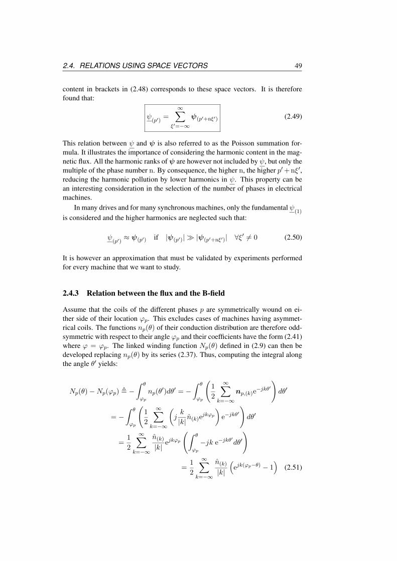
2.4. RELATIONS USING SPACE VECTORS 49
content in brackets in (2.48) corresponds to these space vectors. It is thereforefound that:
ψ(p′)
=
∞∑ξ′=−∞
ψ(p′+nξ′) (2.49)
This relation between ψ and ψ is also referred to as the Poisson summation for-mula. It illustrates the importance of considering the harmonic content in the mag-netic flux. All the harmonic ranks ofψ are however not included by ψ, but only themultiple of the phase number n. By consequence, the higher n, the higher p′+ nξ′,reducing the harmonic pollution by lower harmonics in ψ. This property can bean interesting consideration in the selection of the number of phases in electricalmachines.
In many drives and for many synchronous machines, only the fundamental ψ(1)
is considered and the higher harmonics are neglected such that:
ψ(p′)≈ ψ(p′) if |ψ(p′)| |ψ(p′+nξ′)| ∀ξ′ 6= 0 (2.50)
It is however an approximation that must be validated by experiments performedfor every machine that we want to study.
2.4.3 Relation between the flux and the B-field
Assume that the coils of the different phases p are symmetrically wound on ei-ther side of their location ϕp. This excludes cases of machines having asymmet-rical coils. The functions np(θ) of their conduction distribution are therefore odd-symmetric with respect to their angle ϕp and their coefficients have the form (2.41)where ϕ = ϕp. The linked winding function Np(θ) defined in (2.9) can then bedeveloped replacing np(θ) by its series (2.37). Thus, computing the integral alongthe angle θ′ yields:
Np(θ)−Np(ϕp) , −∫ θ
ϕp
np(θ′)dθ′ = −
∫ θ
ϕp
(1
2
∞∑k=−∞
np,(k)e−jkθ′
)dθ′
= −∫ θ
ϕp
(1
2
∞∑k=−∞
(jk
|k|n(k)e
jkϕp
)e−jkθ
′
)dθ′
=1
2
∞∑k=−∞
n(k)
|k|ejkϕp
(∫ θ
ϕp
−jk e−jkθ′dθ′
)
=1
2
∞∑k=−∞
n(k)
|k|
(ejk(ϕp−θ) − 1
)(2.51)

50 CHAPTER 2. ELECTROMAGNETIC MODEL
Note that according to (2.4), there is no constant coefficient n(0) = 0. Highlightingharmonics and the constant component yields:
Np(θ) =1
2
∞∑k=−∞
(n(k)
|k|ejkϕp
)︸ ︷︷ ︸
Np,(k)
e−jkθ +1
2
(2Np(ϕp)−
∞∑k=−∞
n(k)
|k|
)︸ ︷︷ ︸
Np,(0)
(2.52)
Except for k = 0, the relation between the coefficients of the the coefficients oflinking distribution and the conductor distribution is:
Np,(k) =n(k)
|k|ejkϕp ∀k 6= 0 (2.53)
As shown in the following equations, the magnetic flux (2.10) can then be devel-oped replacing Np(θ) by (2.52), where the constant componentNp,(0) is removed.Since Np,(−k) = N∗p,(k), the sum on k can be substituted by a sum on −k and itis possible to highlight the coefficients B(k) of B(θ) given in (2.36). Introducingψp = ψ(ϕp) given in (2.47) and considering ϕp as a variable, the result is the seriesof the coefficients ψ(k):
ψ(ϕp) = lmR
∮Np(θ)B(θ)dθ = lmR
∮ (1
2
∞∑k=−∞
N∗p,(k)ejkθ
)B(θ)dθ
= lmR
∮ (1
2
∞∑k=−∞
(n(k)
|k|e−jkϕp
)ejkθ
)B(θ)dθ
=1
2
∞∑k=−∞
πlmRn(k)
|k|
(1
π
∮B(θ)ejkθdθ
)︸ ︷︷ ︸
B(k)︸ ︷︷ ︸ψ(k)
e−jkϕp (2.54)
This yields to the relation between the coefficients of the magnetic field and thecoefficients of the magnetic flux:
ψ(k) =πlmR n(k)
|k|B(k) ∀k 6= 0 (2.55)
This relations (2.55) teaches us that the harmonic content of the magnetic B-field flux is filtered through the harmonics of the winding distribution. By con-sequence, it would be incomplete and abusive to speak about machines with sinu-soidal PM-magnetic field, such as the synchronous machines for example, or withtrapezoidal PM-magnetic field, such as BLDC machines for example. If the con-ductor distributions tend toward ideal fundamental sinusoidal functions, i.e. that
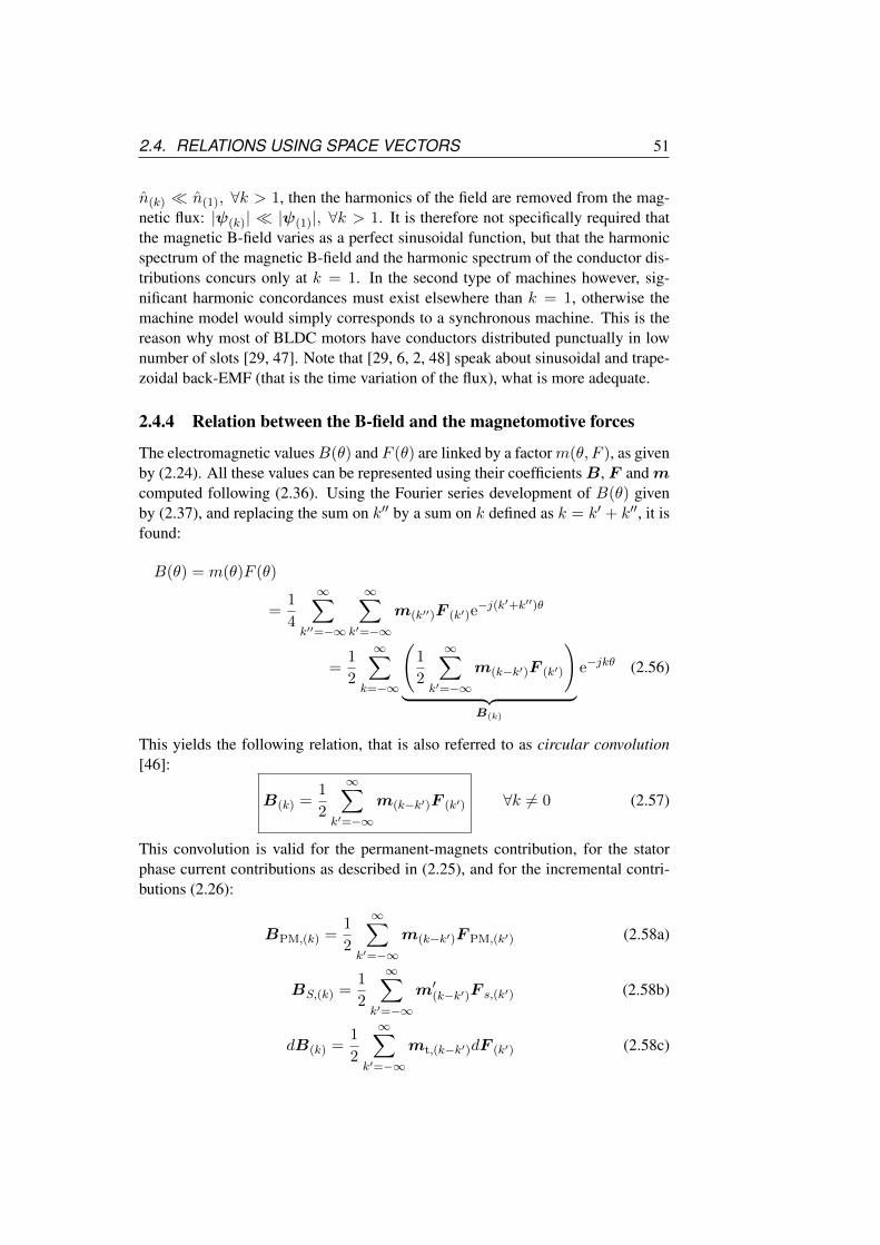
2.4. RELATIONS USING SPACE VECTORS 51
n(k) n(1), ∀k > 1, then the harmonics of the field are removed from the mag-netic flux: |ψ(k)| |ψ(1)|, ∀k > 1. It is therefore not specifically required thatthe magnetic B-field varies as a perfect sinusoidal function, but that the harmonicspectrum of the magnetic B-field and the harmonic spectrum of the conductor dis-tributions concurs only at k = 1. In the second type of machines however, sig-nificant harmonic concordances must exist elsewhere than k = 1, otherwise themachine model would simply corresponds to a synchronous machine. This is thereason why most of BLDC motors have conductors distributed punctually in lownumber of slots [29, 47]. Note that [29, 6, 2, 48] speak about sinusoidal and trape-zoidal back-EMF (that is the time variation of the flux), what is more adequate.
2.4.4 Relation between the B-field and the magnetomotive forces
The electromagnetic valuesB(θ) and F (θ) are linked by a factorm(θ, F ), as givenby (2.24). All these values can be represented using their coefficientsB, F andmcomputed following (2.36). Using the Fourier series development of B(θ) givenby (2.37), and replacing the sum on k′′ by a sum on k defined as k = k′ + k′′, it isfound:
B(θ) = m(θ)F (θ)
=1
4
∞∑k′′=−∞
∞∑k′=−∞
m(k′′)F (k′)e−j(k′+k′′)θ
=1
2
∞∑k=−∞
(1
2
∞∑k′=−∞
m(k−k′)F (k′)
)︸ ︷︷ ︸
B(k)
e−jkθ (2.56)
This yields the following relation, that is also referred to as circular convolution[46]:
B(k) =1
2
∞∑k′=−∞
m(k−k′)F (k′) ∀k 6= 0 (2.57)
This convolution is valid for the permanent-magnets contribution, for the statorphase current contributions as described in (2.25), and for the incremental contri-butions (2.26):
BPM,(k) =1
2
∞∑k′=−∞
m(k−k′)F PM,(k′) (2.58a)
BS,(k) =1
2
∞∑k′=−∞
m′(k−k′)F s,(k′) (2.58b)
dB(k) =1
2
∞∑k′=−∞
mt,(k−k′)dF (k′) (2.58c)

52 CHAPTER 2. ELECTROMAGNETIC MODEL
Remember that dB(k) only models here variations due to dF (k′), while mt,(k−k′)are assumed constant. We see here that the relations between the harmonic contentof the magnetomotive forces and the magnetic B-fields are not straightforward.Since the m factor can be strongly nonlinear, its harmonic spectrum may changewith the magnetic state of the machine. In particular, the harmonic spectra of m,m′ andmt can be very different.
2.4.5 Contribution of the currents to the magnetomotive force
The contribution of the currents to the magnetomotive force Fp(θ) = ipNp(θ) canbe developed replacing Np(θ) by (2.52). Because all coils are identical but shiftedalong their respective angles, the condition Np(ϕp) = N0(ϕ0) ∀p ∈ 1 . . . n− 1can be added to the linking distributions (2.9). We can then highlight the spacevectors i of the currents. It yields:
FS(θ) =n−1∑p=0
ipNp(θ) =n−1∑p=0
ip
(1
2
∞∑k=−∞
Np,(k)e−jkθ
)
=1
2
∞∑k=−∞
n(k)
|k|n
2
2
n
n−1∑p=0
ipejkϕp
︸ ︷︷ ︸
i(k)︸ ︷︷ ︸FS,(k)
e−jkθ +1
2Np,(0)
n
2
2
n
n−1∑p=0
ip
︸ ︷︷ ︸
i(0)︸ ︷︷ ︸F (S,(0))
(2.59)
Finally, the relation between the coefficients F S,(k) of FS(θ) and the space vectorsof the currents is:
F S,(k) =n
2
n(k)
|k|i(k) ∀k 6= 0 (2.60)
It is also valid for incremental contributions. Here also, the harmonic content ofthe magnetomotive force is related to the harmonics in the conductor distributions.
2.4.6 Relation between the flux space vectors and the magnetic sources
Except for the incremental relation, the following relations are given for informa-tion, since they are not used in the self-sensing theory. Combining (2.49) with(2.55) and with (2.58a), the relation between the permanent-magnet contributionto the flux and the contribution to the magnetomotive force yields:
ψPM,(p′)
=∞∑
k′=−∞
∞∑ξ′=−∞
πlmR n(p′+nξ′)
2|p′ + nξ′|m(p′+nξ′−k′)
F PM,(k′) (2.61)

2.4. RELATIONS USING SPACE VECTORS 53
where m are the coefficient of m(θ, FPM, ϕd). Combining (2.58b) with (2.60),the relation between the current contribution to the flux and the contribution to themagnetomotive force yields:
ψS,(p′)
=∞∑
k′=−∞
∞∑ξ′=−∞
πlmR n(p′+nξ′)
2|p′ + nξ′|m′(p′+nξ′−k′)
n
2
n(k′)
|k′|i(k′) (2.62)
where m′ are the coefficient of m′(θ, FPM, FS , ϕd). Note also that there is nomore than n different ranks to i(k). Therefore, the summation on k′ ∈ −∞,∞can be separated by two summations on p ∈ 0,n−1 and ξ ∈ −∞,∞, definedsuch that p+ nξ := k′, and (2.62) yields:
ψS,(p′)
=n−1∑p=0
l(p,p′)i(p) (2.63)
where the self-inductance l(p,p′) is:
l(p,p′) ,nπlmR
4
∞∑ξ′,ξ=−∞
n(p′+nξ′)
|p′ + nξ′|n(p+nξ)
|p+ nξ|m′(p′−p+n(ξ′−ξ)) (2.64)
In a similar way, the relation between the incremental current contribution to theflux and the contribution to the magnetomotive force can be found using (2.58c)and yields:
dψS,(p′)
=n−1∑p=0
lt,(p,p′)di(p) (2.65)
incremental self-inductance lt,(p,p′) is:
lt,(p,p′) ,nπlmR
4
∞∑ξ′,ξ=−∞
n(p′+nξ′)
|p′ + nξ′|n(p+nξ)
|p+ nξ|mt,(p′−p+n(ξ′−ξ)) (2.66)
and wheremt are the coefficient of mt(θ, FPM, FS , ϕd).The factors mt are complex values whose properties regarding the saturation
are inherited by the incremental inductances lt,(p,p′). Their complex form result inan orientation shift between the incremental currents and the incremental fluxes.This shift defines the orientation of the anisotropy. This is developed specificallyfor three-phase machine in the next section.
2.4.7 Electrical torque
The expression of the total torque (2.34) applied on the stator can be developedreplacing the conductor distribution np(θ) by its Fourier series (2.37) in (2.34),
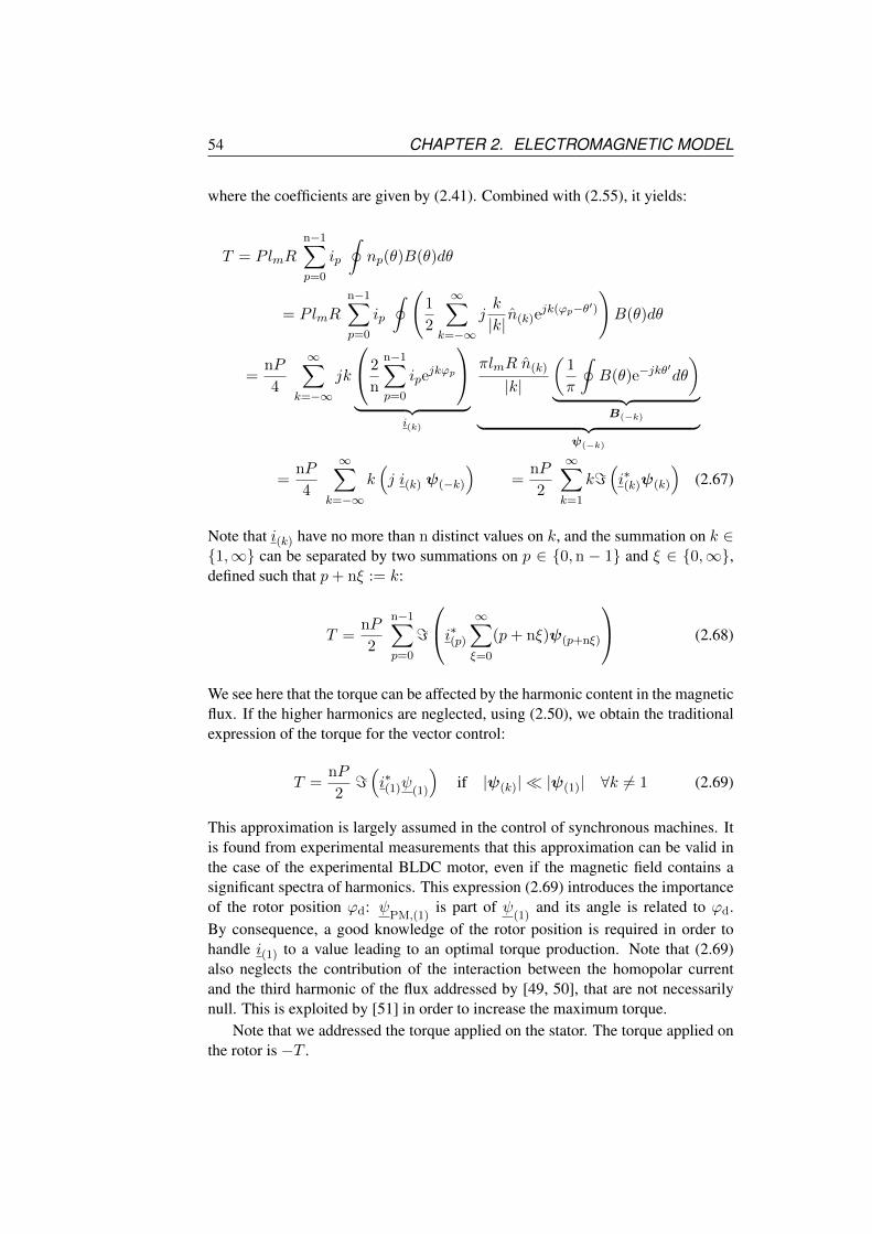
54 CHAPTER 2. ELECTROMAGNETIC MODEL
where the coefficients are given by (2.41). Combined with (2.55), it yields:
T = PlmRn−1∑p=0
ip
∮np(θ)B(θ)dθ
= PlmR
n−1∑p=0
ip
∮ (1
2
∞∑k=−∞
jk
|k|n(k)e
jk(ϕp−θ′)
)B(θ)dθ
=nP
4
∞∑k=−∞
jk
2
n
n−1∑p=0
ipejkϕp
︸ ︷︷ ︸
i(k)
πlmR n(k)
|k|
(1
π
∮B(θ)e−jkθ
′dθ
)︸ ︷︷ ︸
B(−k)︸ ︷︷ ︸ψ(−k)
=nP
4
∞∑k=−∞
k(j i(k) ψ(−k)
)=
nP
2
∞∑k=1
k=(i∗(k)ψ(k)
)(2.67)
Note that i(k) have no more than n distinct values on k, and the summation on k ∈1,∞ can be separated by two summations on p ∈ 0,n − 1 and ξ ∈ 0,∞,defined such that p+ nξ := k:
T =nP
2
n−1∑p=0
=
i∗(p) ∞∑ξ=0
(p+ nξ)ψ(p+nξ)
(2.68)
We see here that the torque can be affected by the harmonic content in the magneticflux. If the higher harmonics are neglected, using (2.50), we obtain the traditionalexpression of the torque for the vector control:
T =nP
2=(i∗(1)ψ(1)
)if |ψ(k)| |ψ(1)| ∀k 6= 1 (2.69)
This approximation is largely assumed in the control of synchronous machines. Itis found from experimental measurements that this approximation can be valid inthe case of the experimental BLDC motor, even if the magnetic field contains asignificant spectra of harmonics. This expression (2.69) introduces the importanceof the rotor position ϕd: ψ
PM,(1)is part of ψ
(1)and its angle is related to ϕd.
By consequence, a good knowledge of the rotor position is required in order tohandle i(1) to a value leading to an optimal torque production. Note that (2.69)also neglects the contribution of the interaction between the homopolar currentand the third harmonic of the flux addressed by [49, 50], that are not necessarilynull. This is exploited by [51] in order to increase the maximum torque.
Note that we addressed the torque applied on the stator. The torque applied onthe rotor is −T .

2.5. THREE-PHASE MACHINES 55
(a) (b)
0xb
ejϕb
ejϕc
xa
xc
ejϕa
32x
0xb
ejϕb
ejϕa
xa
xc x
ejϕc
Figure 2.8: Illustration of (a) the geometrical construction of a space vector x from thephase values xa, xb and xc; (b) and the recovering of the phase values from the spacevector, assuming xo = 0, corresponding to the projections of x along the phase axes.
2.5 Three-Phase Machines
Most of the polyphase machines used in high power applications, such as vehicletraction or power productions, have three phases: n = 3. This choice is historicaland linked to the connection with the three-phase network grid. It has benefits inthe power transportation, minimizing the cost and the loses in cables and in powerelectronics compared to other number of phases. This number should however bereassess in the light of robust control aspects, but it is not done in this work.
2.5.1 Space vector computations
The phases are numbered p ∈ a, b, c for the specific case of n = 3 in thisdocument. Note that many other numbering are found in the literature and thetechnical documents. Using (2.42), the homopolar value xo , x(0)/2 is:
xo ,1
3
∑p=a,b,c
xp (2.70)
Since x(2) = x∗(1), there is only one distinct space vector x(1) in addition to thehomopolar. It is simply referred to as space vector and is written x:
x ,2
3
∑p=a,b,c
xp ejϕp (2.71)
Its geometrical construction is illustrated in Figure 2.8(a). The phase values arefound back using (2.46):
xp = xo + <(x e−jϕp
)(2.72)
It is illustrated in Figure 2.8(b).These computations are valid for any type of connections between the coils,
except the fact that the voltages or the currents at the machine terminals are notnecessarily equal to vp and ip. In a star-connection, ip is well the current flowing

56 CHAPTER 2. ELECTROMAGNETIC MODEL
through the terminals. The voltage at the machine terminals v′p are however equalto the voltage vp at the coil terminals plus the voltage of the neutral point vn:v′p = vp + vn. Since this vn is equal for all the phases, it disappears in the spacevector computation (2.71). This voltage vn should however not be confused withthe homopolar vo, since vo may also contain other internal voltages contributionsin addition to vn. This is specifically true in case of harmonics in the machine.Without neutral connection, the homopolar current is null: io = 0. Note that thevoltage of the neutral point vn is also sometimes called the zero-sequence. In adelta-connection, vp is the difference between the voltage v′p of two consecutivemachine terminals: for example va = v′a − v′b. The current i′p at the machineterminal is divided in the two connected phases: for example i′a = i′a+i′c. This mustbe taken into account in the space vector transformation. Note that the homopolarvoltage vo is not necessarily null due to the back-EMF, whose mean on all thephases is not strictly null in case of harmonics. The homopolar current io is then thecurrent flowing in the delta-loop, also sometimes called the zero-sequence current.
2.5.2 The incremental self-inductances
The restriction to the case of three-phase machine results in strong simplificationsof the relation between the currents and the magnetic flux. Here, we focus on theincremental relation that is used in anisotropy-based self-sensing methods. Theincremental relation (2.65) linking the fundamental space vectors p′ = 1 yields:
dψS
= 2lt,(0,1)dio + lt,(1,1)di+ lt,(2,1)di∗ (2.73)
where the different incremental self-inductances are:
lt,(p,1) =3πlmR
4
∞∑ξ′,ξ=−∞
n(1+3ξ′)
|1 + 3ξ′|n(p+3ξ)
|p+ 3ξ|mt,(1−p+3(ξ′−ξ)) (2.74)
In order to further simplify the relation, assume either that lt,(0,1) = 0 (i.e. n(3ξ′)
∀ξ′), or that there is no homopolar connection io = 0. Both conditions are met inthe case of our experimental motor. By consequence, (2.74) becomes:
dψS
= lt,(1,1)di+ lt,(2,1)di∗ (2.75)
Remember that dψS
only models small variations due to di, while lt,(1,1) and lt,(2,1)
are assumed constant.Following the sames steps, the relation (2.63) yields a similar result for the
current contribution. Assuming either that l(0,1) = 0 or that io = 0, it is found:
ψS
= l(1,1)i+ l(2,1)i∗ (2.76)
This last relation is fundamental for the rotation-drive operations, controlling steady-state values i, but it is not considered in anisotropy-based self-sensing operations.

2.5. THREE-PHASE MACHINES 57
2.5.3 The harmonic incremental self-inductances
The incremental self-inductances are affected by the harmonic spectrum of mt(θ).In order to highlight the harmonic relation, let us define the following inductanceslinked to the kth rank ofmt,(k):
lt,(k) ,3πlmR
4
∞∑ξ′=−∞
n(1+3ξ′)
|1 + 3ξ′|n(1+3ξ′−k))
|1 + 3ξ′ − k|mt,(k) (2.77)
Since mt(θ) is a real function: mt,(−k) = m∗t,(k). Applying a shift on ξ′, it canalso be shown that the sum in (2.77) is symmetrical. By consequence, we have thefollowing property:
lt,(−k) = l∗t,(k) (2.78)
Introducing ξ′′ = ξ − ξ′ and k := 1− p+ 3ξ′′, (2.74) can be written as a develop-ments of these harmonics:
lt,(p,1) =∑
k=1−p+3ξ′′, ∀ξ′′lt,(k) (2.79)
Using the property (2.78), it can be shown that lt,(1,1) is strictly real. This propertyis important in the definition of the anisotropy.
2.5.4 The anisotropy definition
The concept of anisotropy is based on the shift between the space vectors of thecurrents and the fluxes. This shift is directly linked to the complex form of theincremental self-inductance lt,(2,1), while lt,(1,1) is strictly real. At this point, wepropose to introduce some new parameters that correspond to the formalisms metin the literature in case of anisotropy. Let us therefore define the positive lt,+ andnegative lt,- incremental self-inductance, and the anisotropy angle ϕx respectivelyas follows:
lt+ , lt,(1,1) ∈ <
lt- , lt,(2,1) ⇒lt- = |lt-|ϕx , ∠(lt-)/2
(2.80)
where ∠ denotes the complex argument. The positive and negative incrementalself-inductances are sometimes referred to as average and difference inductancesrespectively [52], but this denomination is confusion with concepts further used insignal processing. Thus replacing the inductances in the relation (2.75) by (2.80),we have:
dψS
= lt+di+ lt-di∗ = lt+di+ lt-di
∗ej2ϕx (2.81)
This relation is illustrated in Figure 2.9. For convenience, (2.81) is also furtherwritten in short using a complex factor lt that is function of di (that should not beconfused with the coefficients of the Fourier series):
dψS
= ltdi where lt , lt+ + lt-ej2(ϕx−∠di) (2.82)
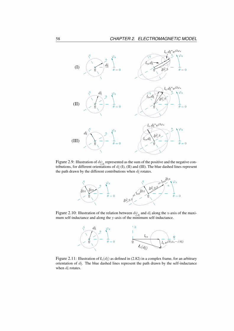
58 CHAPTER 2. ELECTROMAGNETIC MODEL
y
xdi ϕx
θ = 0
lt-di∗ej2ϕx
lt+diϕx
dψ S
y x
θ = 0
y
xϕx
θ = 0
di
lt-di∗ej2ϕx
ϕxy
θ = 0
lt+di
x
dψ S
y
xϕx
di
θ = 0
ϕxx
lt+didψ S
lt-di∗ej2ϕx
θ = 0
(I)
(II)
(III)
0 0
0 0
0 0
Figure 2.9: Illustration of dψS
represented as the sum of the positive and the negative con-tributions, for different orientations of di (I), (II) and (III). The blue dashed lines representthe path drawn by the different contributions when di rotates.
y
di xdi y
xϕx
θ = 0 θ = 0
y ϕx
dψ S,y=ltydi y
dψ S,x=ltxdi x
x
0 0
Figure 2.10: Illustration of the relation between dψS
and di along the x-axis of the maxi-mum self-inductance and along the y-axis of the minimum self-inductance.
y
xdi ϕx
θ = 0
lt(di)
lt-ej2(ϕx−∠di)
=
<lt+
0 0
Figure 2.11: Illustration of lt(di) as defined in (2.82) in a complex frame, for an arbitraryorientation of di. The blue dashed lines represent the path drawn by the self-inductancewhen di rotates.

2.5. THREE-PHASE MACHINES 59
where ∠di is the complex argument of di and thus where di∗ = die−j2∠di. Thisnew factor is illustrated in Figure 2.11.
It is possible to define an anisotropy frame made of two axes denoted x andy, illustrated in Figure 2.10, such that the x-axis is oriented by an angle ϕx withrespect to θ = 0. It is shown that the relation (2.81) is real along the axes of theanisotropy xy-frame and yields:(
dψS,x
dψS,y
)=
(ltx 00 lty
)(dixdiy
)(2.83)
where the inductances ltx and lty are:
ltx = lt+ + lt- & lty = lt+ − lt- (2.84)
such that ltx > lty. Note that the anisotropy xy-frame is here not defined by therotor angle ϕd. The link with the rotor position is introduced after.
Following the sames steps, the relation (2.76) yields a similar result for thecurrent contribution. Transposing (2.80) with l(1,1) and l(2,1) yields:
ψS
= l+i+ l-i∗ = l+i+ l-i
∗ej2ϕx′ (2.85)
where the anisotropy angles may differ: ϕx′ 6= ϕx. Again, this last relation is fun-damental for the rotation-drive operations. It is not considered in anisotropy-basedself-sensing operations, but we however introduce this relation since it appears inthe electromagnetic relations, and it is required to discuss the fact that it can beneglected. This is done in chapter 5.
2.5.5 Impact of the harmonics on the anisotropy
We define the synchronous qd-frame made of two axes denoted q and d such thatthe d-axis is oriented along the permanent-magnets by an angle ϕd. The q-axisis defined here in back-quadrature with respect to the d-axis. From the perspec-tive of anisotropy-based self-sensing, an ideal situation is met if the anisotropyxy-frame is aligned with the synchronous qd-frame. In that case, the estimationof the rotor position is directly obtained from the identification of the anisotropyorientation. Harmonics in the machine however lead to significant misalignmentsbetween these two frames, as explained here.
Assume that contribution of the stator currents FS to the magnetic state is neg-ligible regarding the contribution of the permanent-magnets, such that mt is onlyfunction of FPM oriented by ϕd. As a consequence, mt(θ, FPM, ϕd) is even sym-metric along θ with respect to the angle ϕd and the coefficients mt,(k) have theform (2.40). This form is inherited by lt,(k) defined in (2.77):
mt,(k) = mt,(k)ejkϕd ⇒ lt,(k) = lt,(k)e
jkϕd (2.86)
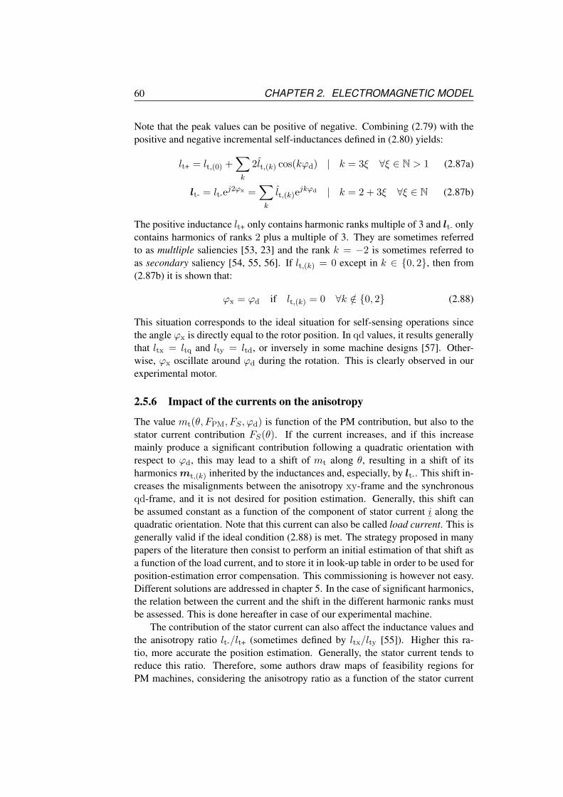
60 CHAPTER 2. ELECTROMAGNETIC MODEL
Note that the peak values can be positive of negative. Combining (2.79) with thepositive and negative incremental self-inductances defined in (2.80) yields:
lt+ = lt,(0) +∑k
2lt,(k) cos(kϕd) | k = 3ξ ∀ξ ∈ N > 1 (2.87a)
lt- = lt-ej2ϕx =
∑k
lt,(k)ejkϕd | k = 2 + 3ξ ∀ξ ∈ N (2.87b)
The positive inductance lt+ only contains harmonic ranks multiple of 3 and lt- onlycontains harmonics of ranks 2 plus a multiple of 3. They are sometimes referredto as multliple saliencies [53, 23] and the rank k = −2 is sometimes referred toas secondary saliency [54, 55, 56]. If lt,(k) = 0 except in k ∈ 0, 2, then from(2.87b) it is shown that:
ϕx = ϕd if lt,(k) = 0 ∀k /∈ 0, 2 (2.88)
This situation corresponds to the ideal situation for self-sensing operations sincethe angle ϕx is directly equal to the rotor position. In qd values, it results generallythat ltx = ltq and lty = ltd, or inversely in some machine designs [57]. Other-wise, ϕx oscillate around ϕd during the rotation. This is clearly observed in ourexperimental motor.
2.5.6 Impact of the currents on the anisotropy
The value mt(θ, FPM, FS , ϕd) is function of the PM contribution, but also to thestator current contribution FS(θ). If the current increases, and if this increasemainly produce a significant contribution following a quadratic orientation withrespect to ϕd, this may lead to a shift of mt along θ, resulting in a shift of itsharmonicsmt,(k) inherited by the inductances and, especially, by lt-. This shift in-creases the misalignments between the anisotropy xy-frame and the synchronousqd-frame, and it is not desired for position estimation. Generally, this shift canbe assumed constant as a function of the component of stator current i along thequadratic orientation. Note that this current can also be called load current. This isgenerally valid if the ideal condition (2.88) is met. The strategy proposed in manypapers of the literature then consist to perform an initial estimation of that shift asa function of the load current, and to store it in look-up table in order to be used forposition-estimation error compensation. This commissioning is however not easy.Different solutions are addressed in chapter 5. In the case of significant harmonics,the relation between the current and the shift in the different harmonic ranks mustbe assessed. This is done hereafter in case of our experimental machine.
The contribution of the stator current can also affect the inductance values andthe anisotropy ratio lt-/lt+ (sometimes defined by ltx/lty [55]). Higher this ra-tio, more accurate the position estimation. Generally, the stator current tends toreduce this ratio. Therefore, some authors draw maps of feasibility regions forPM machines, considering the anisotropy ratio as a function of the stator current

2.6. EXPERIMENTAL BRUSHLESS-DC MOTOR 61
Table 2.1: Design parameters of the experimental motor.Machine length lm 7.1 cm
Stator conductor radius R 12.1 cmAir-gap length δo 5 mm
Pair-pole number P 14PM angle extend ϑ 0.85π
Conductor turns n per pole-pair 4
[58, 59, 60, 61]. They also address the issue of anisotropy misalignment, generallycalled magnetic cross-saturation. These maps are either estimated under commis-sioning, or by finite-element method (FEM) simulations. This is also analyzed in[62] for PM machines, drawing a graph of the anisotropy shift for various currents,or in [63] drawing graphs for a BLDC motor.
Special attention can be given to the machine design in order to increase theiranisotropy ratio. A comparison between machines with buried magnets and surface-mounted magnets is discussed in [58, 59]. A comparison between conventionaland “field-intensified” buried-magnet machines is discussed in [55]. Other “field-intensified PM designs are studied by [64]. An analysis of the influence of thebridge between PM is given by [65]. Similar analysis are proposed in [66], com-paring four types of IM, and in [67], comparing three geometric variations in therotor of IM. Note that it is also possible to increase the some anisotropic propertiesof existing machines by adding a copper turn wound around the poles, as proposedby [68, 69]. The copper turn can be modelled in a similar way to the eddy currentcontributions, as done in the following chapter 3.
2.6 Experimental Brushless-DC Motor
The experimental BLDC motor is a three-phase machine with 14 pairs of surface-mounted permanent-magnets (P = 14) in an outer rotor and three coils at the stator,n = 3, that are connected in star: io = 0. A cross-section is shown in Figure 2.12and an equivalent representation of a single-pole-pair is shown in Figure 2.13. Thecoils of each phase p ∈ a,b, c are made of n conductor turns per pole-pairlocated in single pairs of opposite slots a/a′, b/b′ and c/c′ on either side of theirwinding axes (in a single-pole-pair representation). The P windings of each phaseare connected in series. The permanent-magnets (PM) are mounted on the rotorsurface and centered along the angle ϕd. Each PM covers an angle extent ϑ. Thevalues of the different design parameters are given in Table 2.1. More details onthe design of similar machines can be found in [70].

62 CHAPTER 2. ELECTROMAGNETIC MODEL
stator
rotor
conductor slots
iron stator teeth
permanent-magnets (PM)
ac′ba′
b′
iron rotor armature
hall-effectsensors
c
0
2π
θ
Figure 2.12: Cross-section of the experimental Brushless-DC (BLDC) motor.
ϑϕd
θ = 0δoa′
ac′
b c′
b′
ϕc
ϕb
ϕa
Figure 2.13: Representation the experimental BLDC motor along a single-pole-pair.

2.6. EXPERIMENTAL BRUSHLESS-DC MOTOR 63
k
n(k)
nb(θ)
ϕb = 2π/3
na(θ)
ϕa = 0
nc(θ)
4π/3 = ϕc
0 2 4 6 8 10 12 14 16 18-2-4-6-8-10-12-14-16-18
0
2nπ
− 2nπ
0 90 180
0
3602700 90 180
0
360270
nD
(0)
0 90 180
0
360270 θ
Figure 2.14: Conductor distributions np(θ) and their spectrum n(k) (Fourier coefficients)in a simplified design model.
k
(2.92)
0 2 4 6 8 10 12 14 16 18 20-2-4-6-8-10-12-14-16-18-20
0
n2
24n2/9
Figure 2.15: Values (2.91) as a function of k. The values involved in lt- are mentioned bycircles, in a simplified design model.
2.6.1 Simplified design model
In first approximation, the conductor distributions np(θ) can be modelled by punc-tual values using a delta Dirac function, written here D (it is traditionally writtenδ, but this notation is confusing with the air-gap length):
np(θ) = n(D(θ − ϕp − π/2)−D(θ − ϕp + π/2)
)(2.89)
It is illustrated in Figure 2.14. The Fourier coefficients (2.36) of this distributionare:
np,(k) =1
π
∮np(θ
′)ejkθ′dθ′ = j
2n
πsin(kπ/2) ejkϕp (2.90)

64 CHAPTER 2. ELECTROMAGNETIC MODEL
We have sin(kπ/2) = 0 if k is even, sin(kπ/2) = 1 if k = 1+4ξ and sin(kπ/2) =−1 if k = 3 + 4ξ. Using the form (2.41), the peak values of the harmonics are:
np,(k) = jn(k)k
|k|ejkϕp ⇒ n(k) =
0 if k even2nπ (−1)
|k|−12 if k odd
(2.91)
The spectrum is shown in Figure 2.14. Assuming (2.91), the value of the followingexpression, that is involved in the computation of the inductances lt,(k) (2.77), isgiven in Figure 2.15 as a function of k:
∞∑ξ′=−∞
n(1+3ξ′)
|1 + 3ξ′|n(1+3ξ′−k))
|1 + 3ξ′ − k|(2.92)
where n(1+3ξ′) = 0 for ξ′ odd. The sum can therefore be restricted to n(1+6ξ′), ∀ξ′.In particular, the case k = 0 yields:(
2n
π
)2 ∞∑ξ′=−∞
1
(1 + 6ξ′)2︸ ︷︷ ︸(π/3)2
=4
9n2 (2.93)
while the cases k = 3ξ, ∀ξ > 1 yield 0. As a result, using (2.87a) and using thisprevious computation, it can be checked that the positive inductance lt+ is constantand yields:
lt+ =n2πlmR
3mt,(0) (2.94)
The negative inductance lt-ej2ϕx is not developed analytically, but the nonzero val-
ues of (2.92) involved in (2.87b) are shown by circles in Figure 2.15.Traditionally, in a first approximation of the model of a BLDC motor, the
permanent-magnet contribution to the magnetomotive force distribution FPM(θ)is modelled by a trapezoidal function, as illustrated in Figure 2.16 with the corre-sponding spectrum FPM,(k). This condition is assessed by [29, 6] from the back-EMF point of view. The incremental inductances are very sensitive to the magneticstate between the permanent magnets and this trapezoidal model does not wellmatches with the experimental measurements. We therefore propose to use a rect-angular function, illustrated in Figure 2.17, as suggested by [44]. The real shapeof the distribution is generally more complicated, as suggested by [71] that deeplystudied the magnetic field distribution in BLDC motors.
The air-gap δo is assumed constant, neglecting the slot effects.
Simplified magnetic nonlinearity model
The variation of the factorm(θ) as a function of F (θ) in our experimental machinecannot directly be measured with the available sensors. By consequence, for the
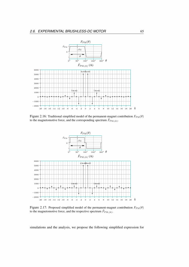
2.6. EXPERIMENTAL BRUSHLESS-DC MOTOR 65
k
FPM,(k) (A)
FPM(θ)
ϑ
ϕd
7.9e+02
5e+035e+03
7.9e+02
0 2 4 6 8 10 12 14 16 18-2-4-6-8-10-12-14-16-18-20 20
−2000
0
1000
2000
3000
4000
5000
6000
−1000
0 90 180 360
0
FPM
240 θ
Figure 2.16: Traditional simplified model of the permanent-magnet contribution FPM(θ)to the magnetomotive force, and the corresponding spectrum FPM,(k).
k
FPM,(k) (A)
FPM(θ)
ϑ
ϕd
3.9e+02
4.9e+034.9e+03
3.9e+02
0 2 4 6 8 10 12 14 16 18-2-4-6-8-10-12-14-16-18-20 20
−2000
0
1000
2000
3000
4000
5000
6000
−1000
0 90 180 360
0
FPM
240 θ
Figure 2.17: Proposed simplified model of the permanent-magnet contribution FPM(θ)to the magnetomotive force, and the respective spectrum FPM,(k).
simulations and the analysis, we propose the following simplified expression for
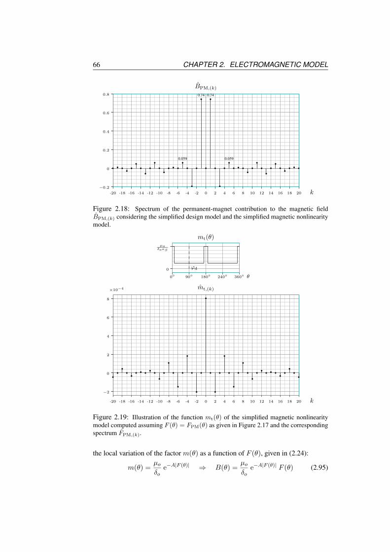
66 CHAPTER 2. ELECTROMAGNETIC MODEL
k
BPM,(k)
0.059
0.74 0.74
0.059
0 2 4 6 8 10 12 14 16 18 20-2-4-6-8-10-12-14-16-18-20
0
0.4
0.2
0.6
0.8
−0.2
Figure 2.18: Spectrum of the permanent-magnet contribution to the magnetic fieldBPM,(k) considering the simplified design model and the simplified magnetic nonlinearitymodel.
k
mt,(k)
mt(θ)
ϕd
0 2 4 6 8 10 12 14 16 18 20-2-4-6-8-10-12-14-16-18-20
0
4
2
6
8
−2
×10−4
0 90 180 360240 θ
0
µoδoκS
Figure 2.19: Illustration of the function mt(θ) of the simplified magnetic nonlinearitymodel computed assuming F (θ) = FPM(θ) as given in Figure 2.17 and the correspondingspectrum FPM,(k).
the local variation of the factor m(θ) as a function of F (θ), given in (2.24):
m(θ) =µoδo
e−A|F (θ)| ⇒ B(θ) =µoδo
e−A|F (θ)| F (θ) (2.95)
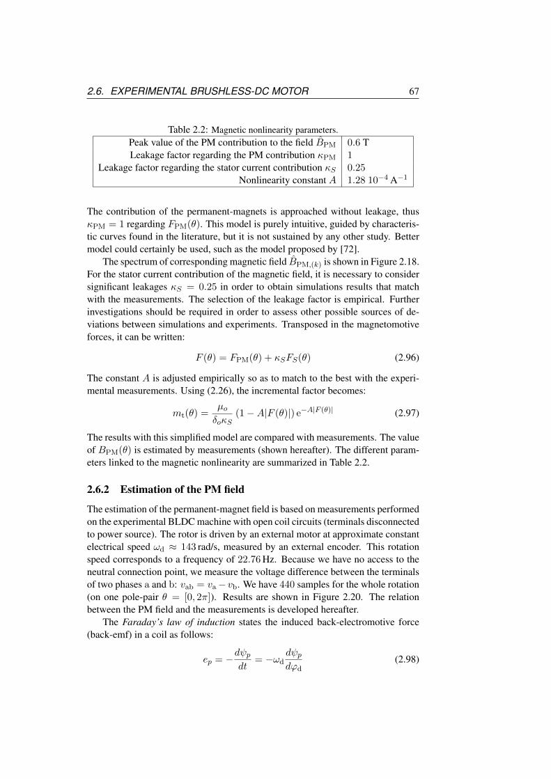
2.6. EXPERIMENTAL BRUSHLESS-DC MOTOR 67
Table 2.2: Magnetic nonlinearity parameters.Peak value of the PM contribution to the field BPM 0.6 TLeakage factor regarding the PM contribution κPM 1
Leakage factor regarding the stator current contribution κS 0.25Nonlinearity constant A 1.28 10−4 A−1
The contribution of the permanent-magnets is approached without leakage, thusκPM = 1 regarding FPM(θ). This model is purely intuitive, guided by characteris-tic curves found in the literature, but it is not sustained by any other study. Bettermodel could certainly be used, such as the model proposed by [72].
The spectrum of corresponding magnetic field BPM,(k) is shown in Figure 2.18.For the stator current contribution of the magnetic field, it is necessary to considersignificant leakages κS = 0.25 in order to obtain simulations results that matchwith the measurements. The selection of the leakage factor is empirical. Furtherinvestigations should be required in order to assess other possible sources of de-viations between simulations and experiments. Transposed in the magnetomotiveforces, it can be written:
F (θ) = FPM(θ) + κSFS(θ) (2.96)
The constant A is adjusted empirically so as to match to the best with the experi-mental measurements. Using (2.26), the incremental factor becomes:
mt(θ) =µoδoκS
(1−A|F (θ)|) e−A|F (θ)| (2.97)
The results with this simplified model are compared with measurements. The valueof BPM(θ) is estimated by measurements (shown hereafter). The different param-eters linked to the magnetic nonlinearity are summarized in Table 2.2.
2.6.2 Estimation of the PM field
The estimation of the permanent-magnet field is based on measurements performedon the experimental BLDC machine with open coil circuits (terminals disconnectedto power source). The rotor is driven by an external motor at approximate constantelectrical speed ωd ≈ 143 rad/s, measured by an external encoder. This rotationspeed corresponds to a frequency of 22.76 Hz. Because we have no access to theneutral connection point, we measure the voltage difference between the terminalsof two phases a and b: vab = va− vb. We have 440 samples for the whole rotation(on one pole-pair θ = [0, 2π]). Results are shown in Figure 2.20. The relationbetween the PM field and the measurements is developed hereafter.
The Faraday’s law of induction states the induced back-electromotive force(back-emf) in a coil as follows:
ep = −dψpdt
= −ωddψpdϕd
(2.98)
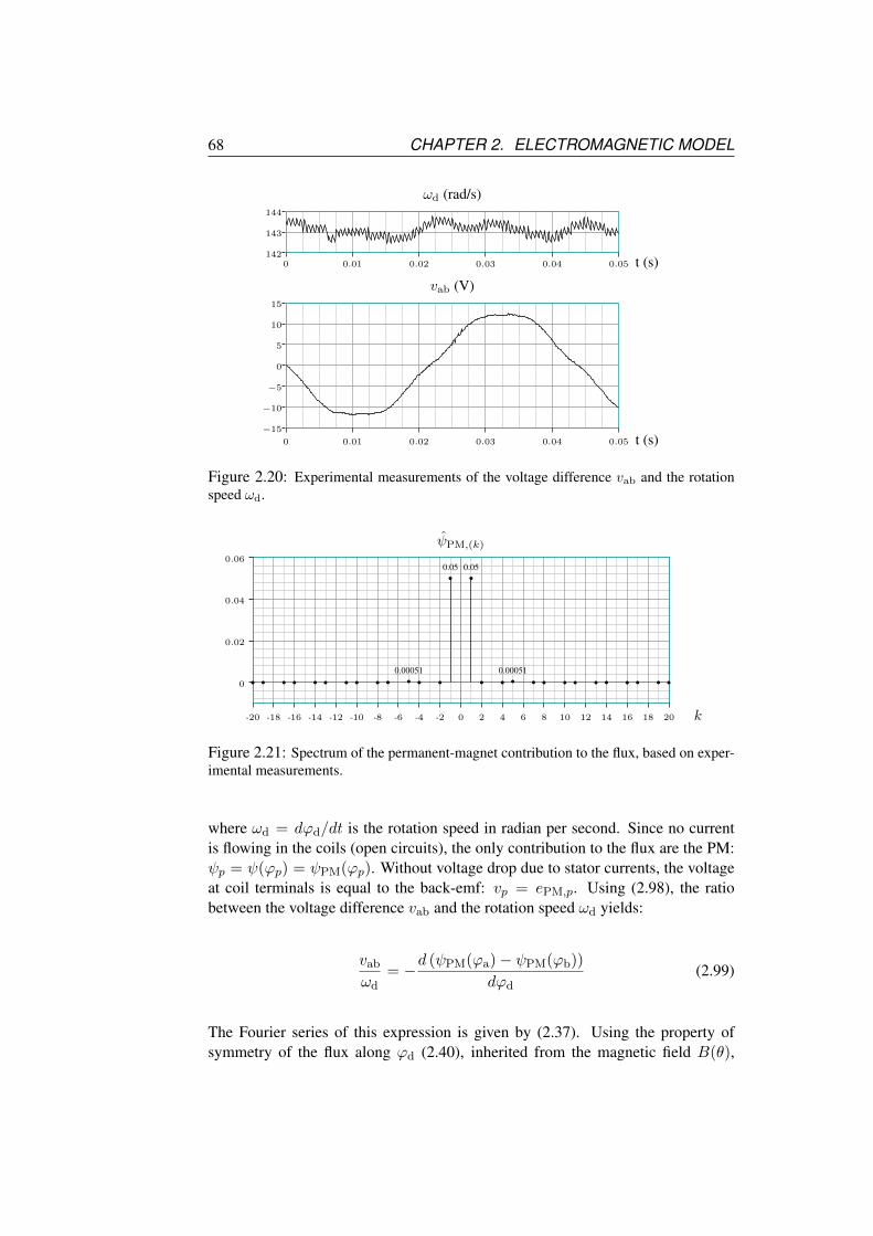
68 CHAPTER 2. ELECTROMAGNETIC MODEL
142
143
144
15
−15
0
−5
−10
5
10
0 t (s)0.050.040.030.020.01
0 t (s)0.050.040.030.020.01
ωd (rad/s)
vab (V)
Figure 2.20: Experimental measurements of the voltage difference vab and the rotationspeed ωd.
k
ψPM,(k)
0.00051
0.05 0.05
0.00051
0 2 4 6 8 10 12 14 16 18 20-2-4-6-8-10-12-14-16-18-20
0
0.04
0.02
0.06
Figure 2.21: Spectrum of the permanent-magnet contribution to the flux, based on exper-imental measurements.
where ωd = dϕd/dt is the rotation speed in radian per second. Since no currentis flowing in the coils (open circuits), the only contribution to the flux are the PM:ψp = ψ(ϕp) = ψPM(ϕp). Without voltage drop due to stator currents, the voltageat coil terminals is equal to the back-emf: vp = ePM,p. Using (2.98), the ratiobetween the voltage difference vab and the rotation speed ωd yields:
vab
ωd= −d (ψPM(ϕa)− ψPM(ϕb))
dϕd(2.99)
The Fourier series of this expression is given by (2.37). Using the property ofsymmetry of the flux along ϕd (2.40), inherited from the magnetic field B(θ),

2.6. EXPERIMENTAL BRUSHLESS-DC MOTOR 69
k
BPM,(k)
0.037
0.73 0.73
0.037
0 2 4 6 8 10 12 14 16 18 20-2-4-6-8-10-12-14-16-18-20
0
0.4
0.2
0.6
0.8
Figure 2.22: Spectrum of the permanent-magnet contribution to the magnetic field, basedon experimental measurements.
(2.37) yields:
ψPM(ϕp) =1
2
∞∑k=−∞
ψPM,(k)e−jkϕp =
1
2
∞∑k=−∞
(ψPM,(k)e
jkϕd
)e−jkϕp
⇒ dψp(ϕp)
dϕd=
1
2
∞∑k=−∞
jkψPM,(k)ejk(ϕd−ϕp) (2.100)
Introducing this expression in (2.99) and using an opposite k order, it yields:
vab
ωd= −1
2
∞∑k=−∞
jkψPM,(k)
(e−jkϕa − e−jkϕb
)ejkϕd
=1
2
∞∑k=−∞
jk(
1− ej2kπ/3)ψPM,(k)︸ ︷︷ ︸
vab
e−jkϕd (2.101)
where ϕa = 0 and ϕb = 2π/3. By consequence, computing the coefficients vab
from the measurements, it is possible to compute ψPM,(k), except on k = 3ξ, ∀ξ,since 1− ej2kπ/3 = 0, but these ranks are not involved in the computations:
ψPM,(k) =vab
jk(1− ej2kπ/3
) ∀k 6= 3ξ, ∀ξ (2.102)
The results are shown in Figure 2.21. The main observation is that the fundamen-tal k = ±1 is very dominant and that the harmonics of ranks k = ±4 are aboutonly 1 % of the fundamental. This suggests that the traditional synchronous vectorcontrol based on (2.50) and (2.69) could be an efficient solution, even if the mag-netic field originally not sinusoidal. Note that part of the spectrum is unknown and

70 CHAPTER 2. ELECTROMAGNETIC MODEL
could be large also. Even if this part is not involved in the vector control, it affectsthe saturation and, by consequence, it affects the inductances. We cannot concludeabout them without further experiments.
Assuming the simplified model of the conductor distribution given in (2.91),assuming no other contribution to the field than the permanent-magnets, and usingthe relation (2.55), we can compute the spectrum of the magnetic field for non-evenk as follows:
B(k) =|k|
πlmR n(k)ψ(k) ∀k odd 6= 3ξ, ∀ξ (2.103)
The results are shown in Figure 2.22. It seems not to be far from the model spec-trum Figure 2.18.
2.6.3 Simulation Results
Simulation of the incremental self-inductance from the simplified models
The negative incremental inductance is computed using (2.87) assuming the sim-plified design model, the simplified magnetic nonlinearity model, and no othercontribution to the field than the permanent-magnets. Using (2.94), the positiveinductance yields:
lt+ = 115.5 µH (2.104)
The negative inductance lt- is computed using (2.87b).
Figures
The results shown in Figure 2.23 and Figure 2.24 are composed of:
• the value lt- in the complex frame ;
• the amplitude lt- = |lt-| as a function of the rotor position ϕd ;
• the anisotropy angle ϕx = 0.5∠(lt-) as a function of the rotor position ϕd ;
• the misalignment shift ϕx−ϕq− 90 as a function of the rotor position ϕd ;
• the harmonic spectrum of lt-.
The 90 shift ofϕx with respect toϕd is due to the fact that the peak value ofmt(θ),illustrated in Figure 2.19, is not along ϕd, but along ϕd − 90. As a consequence,the 2nd rank harmonic lt,(2) is negative. These simulation results are compared tothe results shown in Figure 2.23 assuming an ideal machine defined by (2.88).

2.6. EXPERIMENTAL BRUSHLESS-DC MOTOR 71
k
lt,(k) in lt- (µH)
ϕx − ϕd − 90 (deg)
ϕx = ∠lt-/2 (deg)
lt- = |lt-| (µH)
lt- (µH)
-2.4e-05
0 2 4 6 8 10 12 14 16 18-2-4-6-8-10-12-14-16-18-20 20
−20
0
10
20
−10
−20
0 360180 ϕd60 120 300240
30
0
−30
0 360180 ϕd60 120 300240
180
120
60
0
30
90
150
0 360180 ϕd60 120 3002400
10
20
30
40
0
10
20
40
−10
−20
−30
−40
−40−30 −10 0 10 20 30 40−20
30
0
330
30
6090120
Figure 2.23: Virtual results of lt- for ϕd ∈ [0, 2π], assuming all harmonics are removedexcept lt,(2) (2.88), considering the simplified design model, the simplified magnetic non-linearity model and no other contribution to mt than the permanent-magnets.

72 CHAPTER 2. ELECTROMAGNETIC MODEL
k
lt,(k) in lt- (µH)
ϕx − ϕd − 90 (deg)
ϕx = ∠lt-/2 (deg)
lt- = |lt-| (µH)
lt- (µH)
-4.8e-07 1.5e-06
1.1e-05
-2.4e-05 -3.2e-06 1.6e-07
0 2 4 6 8 10 12 14 16 18-2-4-6-8-10-12-14-16-18-20 20
−20
0
10
20
−10
−20
0 360180 ϕd60 120 300240
30
0
−30
0 360180 ϕd60 120 300240
180
120
60
0
30
90
150
0 360180 ϕd60 120 3002400
10
20
30
40
0
10
20
40
−10
−20
−30
−40
−40−30 −10 0 10 20 30 40−20
30
0
330
30
6090120
Figure 2.24: Values of lt- for ϕd ∈ [0, 2π] and spectrum of its harmonics, consider-ing the simplified design model, the simplified magnetic nonlinearity model and no othercontribution to mt than the permanent-magnets.
2.6. EXPERIMENTAL BRUSHLESS-DC MOTOR 73
Results
In Figure 2.23, the behaviour of lt- is analyzed in the case of an ideal machine,by keeping only the second harmonic rank lt(2) and removing all other ranks. Asa consequence, the shape drawn by lt- during the rotation is a circle. This circleshould not be confused with the circle drawn by lt-e
j2(ϕx−∠di) while di is rotating,illustrated in Figure 2.11. As a consequence, the rotor angle is easily extractedas ϕd = ϕx − 90. In comparison, in the case of our nonideal machine shownin Figure 2.24, the relation between the anisotropy angle ϕx and the rotor angleϕd is affected by significant harmonics. Due to these harmonics, the shape drawnby lt- during the rotation becomes a triangle. An important consequence of theharmonics is the reduction of the accuracy of the rotor angle estimation based onϕx. This estimation is reliable only around some particular angles ξ60 illustratedby crosses in Figure 2.19, while the estimation is inaccurate around angles 30 +ξ60, illustrated by dashed circles.
Simulations analyzing the impact of significant stator currents on the saturationis introduced in [39]. It is however not presented here because the model couldnot be validated at rated load. This would require further investigations and animproved test bench.
2.6.4 Experimental Results
Estimations of the incremental self-inductance from experiments
The experiments are performed on the standstill experimental BLDC motor, withthe rotor blocked at 127 different positions between ϕd = 0 and 360. At each ro-tor position, the incremental self-inductances are computed based on 2× 100 sam-ples taken with a voltage pulse instructions dv of 0.77 V amplitude injected duringperiods of Ts = 0.1 ms along two different directions, such that they produce fluxvariations dψS = dv/Ts of 7700 Wb amplitude. The current variations di relatedto these flux variations are between 0.7 A and 1.4 A, depending the orientation withrespect to the anisotropy. They are measured by a current sensors with a 0.244 Aresolution. This low resolution constitutes the main source of noise (digital noise)and the standard deviation of the current measurements is thus around half the sen-sor resolution. The noise issue is further addressed in section 5.3. Due to the lowratio of the current variations on the standard deviation, that is between 10 and 20,the standard deviation on the self-inductances is also quite large, between 5µH and13µH. The impact of this deviation is however reduced by 10 computing the meanof the results on 100 samples. Assuming a computation method based on thesemean values, the error on self-inductances lt+ and lt- should be around 2µH, andthe error on the angle ϕd is around 2.5. The resolution step of the encoder, mea-suring the rotor position, is 8192 on a whole rotation, thus 8192/P/360 = 1.6
on ϕd.

74 CHAPTER 2. ELECTROMAGNETIC MODEL
k
l t-
=|l t
-|(µ
H)
l t-
(µH
)
ϕx
=∠l t
-/2
(deg
)−
90
(deg
)ϕ
x−ϕ
d
l t,(k)
inl t
-(µ
H)
l t+
(µH
)
2.9e-06 5.5e-07
2.5e-07
-1.7e-05
0 2 4 6 8 10 12 14 16 18-2-4-6-8-10-12-14-16-18-20 20
−20
0
10
20
−10
−20
0 360180 ϕd60 120 300240
30
0
−30
0 360180 ϕd60 120 300240
180
120
60
0
30
90
150
0 360180 ϕd60 120 3002400
10
20
30
40
0
10
20
40
−10
−20
−30
−40
−40−30 −10 0 10 20 30 40−20
30
0
330
30
6090120
0 360180 ϕd60 120 30024060
70
80
90
Figure 2.25: Experimental values of lt- for ϕd ∈ [0, 2π] and spectrum of its harmonics,with i = 0 A.

2.6. EXPERIMENTAL BRUSHLESS-DC MOTOR 75
k
l t-
=|l t
-|(µ
H)
l t-
(µH
)
ϕx
=∠l t
-/2
(deg
)−
90
(deg
)ϕ
x−ϕ
d
l t,(k)
inl t
-(µ
H)
l t+
(µH
)
3.8e-06
-2e-05
-1.5e-06
-4.3e-06
0 2 4 6 8 10 12 14 16 18-2-4-6-8-10-12-14-16-18-20 20
−20
0
10
20
−10
−20
0 360180 ϕd60 120 300240
30
0
−30
0 360180 ϕd60 120 300240
180
120
60
0
30
90
150
0 360180 ϕd60 120 3002400
10
20
30
40
0
10
20
40
−10
−20
−30
−40
−40−30 −10 0 10 20 30 40−20
30
0
330
30
6090120
0 360180 ϕd60 120 30024060
70
80
90
Figure 2.26: Experimental values of lt- for ϕd ∈ [0, 2π] and spectrum of its harmonics,with i = 36 A ejϕq .

76 CHAPTER 2. ELECTROMAGNETIC MODEL
∠(−lt,(2))
2 (deg)
∠(lt,(−4))
−4 (deg)|lt,(−4)| (µH)
|lt,(2)| (µH)
|lt,(0)| (µH)
0 3612 24−2 |i| (A)
0
2
4
6
8
0 3612 24−2 |i| (A)
0
2
4
6
8
0 3612 2416 |i| (A)
21
19
17
20
18
0 3612 24
3
|i| (A)
4
0 3612 2475 |i| (A)
80
78
76
77
79
Figure 2.27: Experimental values of the load impact on the harmonic ranks k = 2,−4,involved in lt-, and on the harmonic rank k = 0, involved in lt+.
Figures
Results are shown in Figure 2.25 and Figure 2.26, respectively for a no-load sit-uation (i = 0) and for a loaded situation (i = 36 A along the q-axis). They arecomposed as follows:
• the value lt- in the complex frame ;
• the amplitude lt- = |lt-| as a function of the rotor position ϕd ;
• the anisotropy angle ϕx = 0.5∠(lt-) as a function of the rotor position ϕd ;
• the misalignment shift ϕx−ϕq− 90 as a function of the rotor position ϕd ;
• the harmonic spectrum of lt-, with real values shown by dots and imaginaryvalues shown by small squares ;
• the value lt+ as a function of the rotor position ϕd.
Results
As we can see, Figure 2.25 is in good agreement with the simulation result Fig-ure 2.24. The main difference concerns the harmonic spectrum where only the
2.7. SUMMARY 77
ranks k = 2 and k = −4 present significant values. Concerning the self-sensingopportunities, compared to the previous conclusion based on simplified models,this experimental result suggests that it could be possible to increase the resolutionof the rotor position estimation by taking only these second harmonics, of rankk = −4, into account. This is however not done is thesis due to lack of time. Aswe can see in Figure 2.26, the increase of the load (stator current along the q-axis)produces a shift in the anisotropy angle. This is observed in the spectral contentof lt-, computed with respect to the angle ϕd given by the encoder. The positiveinductance lt+ is also slightly increased.
Figure 2.27 shows the load impacts, measured for |i| = 0, 12, 24, 36 A alongthe q-axis, on different harmonic ranks k = 2,−4, involved in lt-, and on theharmonic rank k = 0, involved in lt+. This impact is rather large and will certainlycontinuously increase up to the rated 134 A. If a linear behaviour is assumed, theanisotropy shift would reach 26. Observe that the ranks 2 and −4 that are shiftedby similar angles. This suggests that they are affected in a similar way by theload. Many papers propose to compensate for this load shift performing an offlinecommissioning. This commissioning however requires a specific test bench witha rotor position sensor and with a blocked rotor up to the maximum load. In thecase of our experimental motor, the rated torque is 150 Nm. This is quite large andthis experiment was not performed at this stage of the study. Different solutionsare addressed in chapter 5.
2.7 Summary
In this chapter, we introduced the general electromagnetic model of the PM electricmachine. Several assumptions were however required:
• machine made of cylindrical parts without magnetic field flowing throughthe edges, with as a consequence the exclusion of any axial component inthe magnetic field ;
• symmetrically wounded coils on either side of their phase angles ϕp, plusthe assumption of identical coils ;
• no homopolar current.
Large developments for any number of phases were proposed, offering tools forthe study and the control of polyphase machines. We however focus on three-phase machine and the principal expressions to keep in mind for the rest of thisthesis are:
• the computation of the fundamental complex space vector (2.71) for three-phase machines ;
• the expression of the torque (2.69) neglecting the harmonics ;

78 CHAPTER 2. ELECTROMAGNETIC MODEL
• the expression of the anisotropic incremental relation (2.81) in three-phasemachines.
The experimental BLDC motor has been analyzed through simulations and exper-iments. The main experimental results are:
• Figure 2.21 shows that the magnetic flux contains harmonics of rank k = 5that is only 1 % the fundamental k = 1. We propose therefore to neglectthese harmonics in the torque expression and to perform a field-oriented con-trol generally applied on PMSM, as further described in chapter 5 ;
• Figure 2.25 and Figure 2.26 illustrate the oscillating error due to harmonicsin the machine, and show that the negative self-inductance, used to obtainedthe anisotropy angle ϕx, contains harmonics of rank k = −4, referred toas second harmonics, while the other harmonics ranks are rather negligi-ble. This would limit the complexity of the development of a compensationmethod (not done in this thesis) ;
• Figure 2.27 finally illustrated the significant impact of the stator currents.
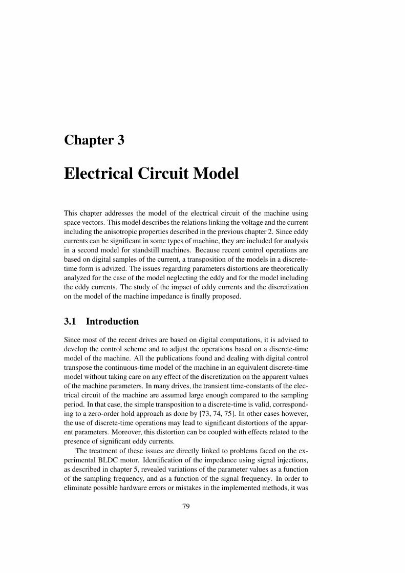
Chapter 3
Electrical Circuit Model
This chapter addresses the model of the electrical circuit of the machine usingspace vectors. This model describes the relations linking the voltage and the currentincluding the anisotropic properties described in the previous chapter 2. Since eddycurrents can be significant in some types of machine, they are included for analysisin a second model for standstill machines. Because recent control operations arebased on digital samples of the current, a transposition of the models in a discrete-time form is advized. The issues regarding parameters distortions are theoreticallyanalyzed for the case of the model neglecting the eddy and for the model includingthe eddy currents. The study of the impact of eddy currents and the discretizationon the model of the machine impedance is finally proposed.
3.1 Introduction
Since most of the recent drives are based on digital computations, it is advised todevelop the control scheme and to adjust the operations based on a discrete-timemodel of the machine. All the publications found and dealing with digital controltranspose the continuous-time model of the machine in an equivalent discrete-timemodel without taking care on any effect of the discretization on the apparent valuesof the machine parameters. In many drives, the transient time-constants of the elec-trical circuit of the machine are assumed large enough compared to the samplingperiod. In that case, the simple transposition to a discrete-time is valid, correspond-ing to a zero-order hold approach as done by [73, 74, 75]. In other cases however,the use of discrete-time operations may lead to significant distortions of the appar-ent parameters. Moreover, this distortion can be coupled with effects related to thepresence of significant eddy currents.
The treatment of these issues are directly linked to problems faced on the ex-perimental BLDC motor. Identification of the impedance using signal injections,as described in chapter 5, revealed variations of the parameter values as a functionof the sampling frequency, and as a function of the signal frequency. In order toeliminate possible hardware errors or mistakes in the implemented methods, it was
79

80 CHAPTER 3. ELECTRICAL CIRCUIT MODEL
1 = eϕα , eϕaβ
j = eϕβ , eϕa+π/2
α
(a)
0 0 xα = <(x)
∠xx=(x) = xβ
(b)
Figure 3.1: (a) Unitary space vectors of the stationary αβ-frame ; and (b) illustration of aspace vector x and its axis components in the stationary αβ-frame.
required to compare these results with simulations based on adequate models. Itwas firstly revealed that the simple modelling considering the discretization, butneglecting eddy currents gave unsatisfying results. Another model, much morecomplicated and including the eddy currents, was therefore developped. This newmodel offered very satisfying simulations results in adequacy with the experiments.For complexity reasons, the model was however restricted to standstill machines.
A significant part of this chapter addressed the mathematical development ofthe model discretization taking the eddy currents into account. This work allowedto concluded that the eddy current were the cause of the parameter distortion, ex-cluding any cause from the hardware or the implementation.
∼
This chapter is organized as follows: the section 3.2 introduces general rela-tions with space vectors in different reference-frames ; Section 3.3 describes theelectrical model in case of anisotropic relations firstly neglecting the eddy current,and secondly including the eddy currents ; Section 3.4 substitutes the continuous-time models by equivalent discrete-time models. The impact of the two-levelthree-phase pulse-width modulated voltage source inverter on this discretization islargely developped, assuming a standstill motor ; Section 3.5 introduces the modelunder the form of impedances, since the impedance is the value identified by theself-sensing method proposed in chapter 5. Comparisons between measurementson the experimental machines and model results confirm the validity of the mod-els ; A summary of the important elements of this chapter is given in section 3.6.
3.2 Space Vectors in Different Frames
3.2.1 The Stationary Frame
Using complex space vectors
Assume a set of 3 phase values, written xp where p ∈ a,b, c, related to anelectromagnetic phenomenon occurring in the different stator phase-coils of themachine. This phenomenon can be the voltage applied to the coil terminals vp, thecurrent flowing in the phase coils ip, the magnetic flux linked by the phase coilsψp. The complex space vector x is defined in (2.71) of the chapter 2 as the phase

3.2. SPACE VECTORS IN DIFFERENT FRAMES 81
contributions xp along the conductor orientations ϕp ; and the homopolar xo isdefined in (2.70) as the sum of the phase values xp:
x ,2
3
∑p=a,b,c
xp ejϕp and xo ,1
3
∑p=a,b,c
xp (3.1)
where ϕa = 0, ϕb = 2π/3 and ϕc = 4π/3. The phase values are found back using(2.46):
xp = xo + <(x e−jϕp
)∀p ∈ a, b, c (3.2)
Being defined with respect to the stator phase-coils, it is said that this space vectorx is in the stationary frame. As illustrated in Figure 3.1, this stationary frame isgenerally identified by two orthogonal axes: one axis α is oriented along the firstphase a, i.e. by an angle ϕα = ϕa, and the other axis β is oriented in quadrature,i.e. by an angle ϕα = ϕa + π/2. Since ϕa = 0, the axis α is thus also the axis ofthe real values and β is the axis of the imaginary values, with the following unitaryspace vectors: ejϕα = 1 and ejϕβ = j. The real and imaginary components of xare thus linked to the axes as follows:
xα , <x and xβ , =x ⇔ x = xα + jxβ (3.3)
The matrix relations
Combining (3.2) with (3.3) yields the matrix relation between the αβ-componentsof the space vector, plus the homopolar, and the phase values as follows: xa
xb
xc
=
cos(ϕa) sin(ϕa) 1cos(ϕb) sin(ϕb) 1cos(ϕc) sin(ϕc) 1
︸ ︷︷ ︸
C
xαxβxo
(3.4)
This computation is often referred to as the Clark-transformation. It can be re-versed and yields: xα
xβxo
=2
3
cos(ϕa) cos(ϕb) cos(ϕc)sin(ϕa) sin(ϕb) sin(ϕc)
0.5 0.5 0.5
︸ ︷︷ ︸
C−1
xa
xb
xc
(3.5)
The same result can be obtained combining (3.1) with (3.3).
Using matrix space vectors
In many papers of the literature, the term “space vector” refers to the matrix con-taining the components along the frame axes. To make the difference with the
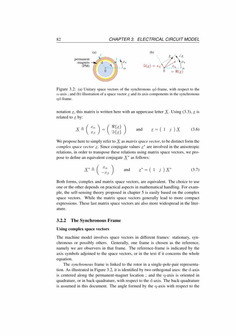
82 CHAPTER 3. ELECTRICAL CIRCUIT MODEL
0 = <(x)
x
=(x) = xd
∠x
α
ϕq
(b)
xqq
d
α
j(a)
1ϕq
0
permanent-magnets
(PM)
Figure 3.2: (a) Unitary space vectors of the synchronous qd-frame, with respect to theα-axis ; and (b) illustration of a space vector x and its axis components in the synchronousqd-frame.
notation x, this matrix is written here with an uppercase letter X . Using (3.3), x isrelated to x by:
X ,
(xαxβ
)=
(<x=x
)and x =
(1 j
)X (3.6)
We propose here to simply refer toX as matrix space vector, to be distinct form thecomplex space vector x. Since conjugate values x∗ are involved in the anisotropicrelations, in order to transpose these relations using matrix space vectors, we pro-pose to define an equivalent conjugate X∗ as follows:
X∗ ,
(xα−xβ
)and x∗ =
(1 j
)X∗ (3.7)
Both forms, complex and matrix space vectors, are equivalent. The choice to useone or the other depends on practical aspects in mathematical handling. For exam-ple, the self-sensing theory proposed in chapter 5 is easily based on the complexspace vectors. While the matrix space vectors generally lead to more compactexpressions. These last matrix space vectors are also more widespread in the liter-ature.
3.2.2 The Synchronous Frame
Using complex space vectors
The machine model involves space vectors in different frames: stationary, syn-chronous or possibly others. Generally, one frame is chosen as the reference,namely we are observers in that frame. The reference-frame is indicated by theaxis symbols adjoined to the space vectors, or in the text if it concerns the wholeequation.
The synchronous frame is linked to the rotor in a single-pole-pair representa-tion. As illustrated in Figure 3.2, it is identified by two orthogonal axes: the d-axisis centered along the permanent-magnet location ; and the q-axis is oriented inquadrature, or in back-quadrature, with respect to the d-axis. The back-quadratureis assumed in this document. The angle formed by the q-axis with respect to the

3.2. SPACE VECTORS IN DIFFERENT FRAMES 83
α-axis is written ϕq. As reference-frame, the q-axis becomes the axis of the realvalues and the d-axis becomes the axis of the imaginary values.
It is possible to switch the reference frame from the stationary αβ-frame to theqd-frame, applying a negative rotation on the space vector by the angle ϕq of theq-axis with respect to the α-axis:
x|qd = e−jϕq x|αβ (3.8)
Time derivatives of space vectors are involved in the model. It is therefore con-venient to introduce the expression linking the time derivative of a space vector indifferent reference-frames. Using (3.8), in the qd reference-frame, it yields:
e−jϕqdx|αβdt
=dx|qd
dt+ jωq x|qd (3.9)
where ωq = dϕq/dt. Observe that the change from the stationary αβ reference-frame to the synchronous qd reference-frame introduce a term related to the speedbetween the reference-frames.
Using matrix space vectors
Handling the matrix space vectors (3.6) in the respective reference-frames, the re-lation (3.8) yields:
X|qd =
(cos(ϕq) sin(ϕq)− sin(ϕq) cos(ϕq)
)X|αβ (3.10)
and the relation (3.9) yields:(cos(ϕq) sin(ϕq)− sin(ϕq) cos(ϕq)
)dX|αβdt
=dX|qd
dt+ ωq
(0 −11 0
)︸ ︷︷ ︸
J
X|qd (3.11)
where we introduced the matrix J substituting the imaginary unity j.
The matrix relations including the homopolar
It is possible to link the axes components, plus the homopolar xo, with the phasevalues directly by matrix referred to as Park transformations. This is found com-bining (3.4) and (3.5) with (3.10), and yields: xa
xb
xc
= C
cos(ϕq) − sin(ϕq) 0sin(ϕq) cos(ϕq) 0
0 0 1
xq
xd
xo
(3.12)
and xq
xd
xo
=
cos(ϕq) sin(ϕq) 0− sin(ϕq) cos(ϕq) 0
0 0 1
C−1
xa
xb
xc
(3.13)

84 CHAPTER 3. ELECTRICAL CIRCUIT MODEL
α
y
y
b-x
a+ej2ϕxx∗
x ϕxx
βy
x
α
ϕx
00
Figure 3.3: Illustration of the anisotropic relation between two space vectors x and yfollowing (3.14), and the related anisotropy xy-frame.
These matrix transformations are given for information, but they will not be furtherused. We prefer to compute the space vectors using the initial definition (3.1)and then to handle them in the synchronous reference frame using complex spacevectors (3.8) or matrix space vectors (3.10).
3.2.3 The Anisotropic Relation
Using complex space vectors
In a general way, an anisotropic relation between two space vectors x and y isdefined in the stationary αβ reference-frame by the following form:
y = a+x+ a-x∗
= a+x+ a-ej2ϕxx∗
where
a+ ∈ <
a- ∈ = ⇒a- = |a-| ∈ <ϕx , ∠(a-)/2
(3.14)
where a+ and a- are called the positive and negative parameters respectively, andϕx is called the anisotropy angle. This angle gives the orientation of the relatedxy frame with respect to the reference-frame. This is illustrated in Figure 3.3. Therelation between the linked flux and the current contributions (2.81) and (2.85),addressed in chapter 2, satisfy to this definition of the anisotropy.
Using (3.8), and since x∗|qd = ejϕq x∗|αβ , the anisotropic relation (3.14) trans-posed in the synchronous qd reference-frame yields:
y = a+x+ a-e−j2ϕqx∗
= a+x+ a-ej2(ϕx−ϕq)x∗
(3.15)
If the synchronous qd frame is aligned with the anisotropy xy frame, we haveϕx = ϕq and (3.15) yields:
y = a+x+ a-x∗ (3.16)
We see hereafter how these relations appear using the matrix space vectors.

3.2. SPACE VECTORS IN DIFFERENT FRAMES 85
Using matrix space vectors
Handling matrix space vectors (3.6) and (3.7), the relation (3.14) in the stationaryαβ reference-frame yields:
Y = a+X + a-
(cos(2ϕx) − sin(2ϕx)sin(2ϕx) cos(2ϕx)
)X∗ (3.17)
This result can also be written as a matrix relation between X and Y :
Y =
(aαα aαβaαβ aββ
)︸ ︷︷ ︸
A
X ⇒
aαα = a+ + a- cos(2ϕx)aββ = a+ − a- cos(2ϕx)aαβ = a- sin(2ϕx)
(3.18)
For information, reversing it, yields:
a+ =aαα + aββ
2and a- = a-e
j2ϕx =aαα − aββ
2+ jaαβ (3.19)
This relation can be used to compute the parameters of the space vector relationfrom the knowledge of the matrix A.
The relation (3.15) in the synchronous qd reference-frame yields:
Y =
(aqq aqd
aqd add
)X ⇒
aαα = a+ + a- cos(2(ϕx − ϕq))aββ = a+ − a- cos(2(ϕx − ϕq))aαβ = a- sin((ϕx − ϕq))
(3.20)
If the synchronous qd frame is aligned with the anisotropy xy frame, we haveϕx = ϕq and (3.20) yields:
Y =
(a+ + a- 0
0 a+ − a-
)X (3.21)
where ax = a+ +a- and ay = a+−a- are respectively the maximum and minimumvalues of the parameter.
Since the matrix (3.21) is diagonal, it is said that the relation along the x andthe y axes is uncoupled. A contrario, the matrix (3.20) is not diagonal if thesynchronous and anisotropy frames are misaligned. In that case, it is said thatthe q and the d axes cross-coupled. These terms of “saturation cross-coupling”[76, 63, 59, 55] or “cross-saturation” [54, 77, 60] or “cross-magnetization” [78]are often addressed in literature concerning the position self-sensing strategies. Wesee however that these coupling effects are only a point of view depending on theconsidered reference-frame. Generally, the coupling is assessed with respect tothe qd frame and, thus, simply qualifies the fact that the synchronous qd frame ismisaligned with the anisotropy.

86 CHAPTER 3. ELECTRICAL CIRCUIT MODEL
3.3 Continuous-time models
3.3.1 Induced Voltages
The Faraday’s law of induction states that the time derivative of the flux ψ linkedby the phase coils induces a voltage e in the machine circuits. This relation is statedin the reference-frame of the linking coils, that is the stationary αβ-frame. In thatframe, the relation can be written:
e =dψ
dt(3.22)
In a permanent-magnet machine, the flux ψ can be separate in three main contri-butions:
ψ = ψS
+ ψPM
+ ψE
(3.23)
1. a self-contribution from the stator currents i, written ψS
, that is possiblynonlinear (since the relation depends on the magnetic state of the machineand therefore varies as a function of the different magnetic sources) and pos-sibly anisotropic (due to rotor geometry variations or to magnetic saturationeffects) ;
2. the contribution from the permanent magnets (PM), written ψPM
, that bydefinition only depends on the PM contribution to the magnetic state of themachine. Since the magnetomotive force (mmf) of the PM is assumed con-stant along the rotor-side, ψ
PMhas a constant amplitude and is oriented as a
function of the PM position ϕd ;
3. the contribution from eddy currents iE appearing in the iron of the machine,written ψ
E, that is further discussed.
The respective induced voltages are eS , ePM and eE, such that: e = eS+ePM +eE.In addition, the Ohm’s law states that the electrical current i flowing through thephase coils produce a voltage drop vr by a factor of resistance, introduced hereafter.The supply voltage v applied to the coil terminals is then equal to the inducedvoltage e plus the voltage drop vr:
v = vr + e = vr + eS + ePM + eE (3.24)
These different voltages are developed hereafter. Note that we often switch be-tween complex and matrix space vectors, since both are useful.
3.3.2 The Resistive Voltage Drop
The relation between the voltage drop vr and the current i can reveal an anisotropicproperty, as defined by (3.14), due to unbalancing between the resistances of the

3.3. CONTINUOUS-TIME MODELS 87
different stator coils. This is shown as follows. The resistive voltage drop vr,p ofthe different phases p can be written in a matrix form as: vr,a
vr,bvr,c
=
ra 0 00 rb 00 0 rc
︸ ︷︷ ︸
Rabc
iaibic
(3.25)
Using the Clack matrices (3.4) and (3.5), it is possible to compute the equivalentrelation between the space vector components in the stationary frame, plus thehomopolar, as follows: vr,α
vr,βvr,o
=
rαα rαβ rαorβα rββ rβoroα roβ roo
︸ ︷︷ ︸
Rαβo
iαiβio
(3.26)
where Rαβo = C−1RabcC
=2
3
ra + 12(rb + rc)
√3
4 (rc − rb) ra − 12(rb + rc)√
34 (rc − rb) 3
4(rc + rb)√
32 (rb − rc)
12ra − 1
4(rb + rc)√
34 (rb − rc)
12(ra + rb + rc)
(3.27)
We firstly observe that there is an interaction between the homopolar current ioand the voltage drops vr,α and vr,β in the stationary frame through rαo and rβo thatare possibly not null. Since there are no neutral connection in our experimentalmachine, we propose to assumed the case io = 0 and to ignore this interaction.Thus using matrix space vectors (3.6), the relation (3.26) yields:
V r =
(rαα rαβrβα rββ
)︸ ︷︷ ︸
R
I (3.28)
We secondly observe that the interaction between the two axes is reciprocal: rαβ =rβα. Thanks to this reciprocity, (3.28) has the form of an anisotropic relation in itsmatrix form (3.18). Computing r+ and r- as given in (3.19), (3.28) can be writtenwith complex space vectors as given in (3.14) in the stationary reference-frame:
vr = r+i+ r-i∗ (3.29)
It is important to note that the orientation of this resistive anisotropy, i.e. ∠(r-)/2,is only function of the phase resistances, but does not contain any rotor positioninformation.

88 CHAPTER 3. ELECTRICAL CIRCUIT MODEL
3.3.3 Back-electromagnetic force
Approximations for a synchronous machine
The back-electromagnetic force (back-emf) is the contribution from the PM to theinduce voltage, written ePM. Assume that the the contribution from the PM is onlyfunction of the PM angle ϕd. Thus we can write in the stationary αβ-frame:
ePM =dψ
PM
dt= ωd
∂ψPM
∂ϕd(3.30)
where ωd = dϕd/dt. The expression (3.30) in the synchronous qd reference-frameis found using (3.9) and yields:
ePM =dψ
PM
dt+ jωdψPM
= ωd
(∂ψ
PM
∂ϕd+ jψ
PM
)(3.31)
where ωq = ωd.Assume that ψ
PMcan be approached as a space vector oriented along the d-
axis. In the stationary reference-frame, (3.30) yields:
ψPM
= |ψPM|ejϕd ⇒
∂ψPM
∂ϕd= jψ
PM⇒ ePM = jωdψPM
(3.32)
In the synchronous reference-frame, we have:
ψPM
= |ψPM|ejϕde−jϕq = |ψ
PM|ejπ/2 ⇒
∂ψPM
∂ϕd= 0 (3.33)
And thus, (3.30) yields the same expression as (3.32).
3.3.4 Current Contribution To The Induced Voltage
Assume that the contribution from the stator current is function not only of thestator currents i, but also of the PM angle ϕd. Thus, using ϕq = ϕd− π/2, we candevelop the induced voltage in the stationary αβ reference-frame as follows:
eS =dψ
S
dt=∂ψ
S
∂i
di
dt+ ωq
∂ψS
∂ϕq(3.34)
Note that ωq = ωd. The partial derivative on the angle ϕq is found assuming aconstant current, i.e. it is found around the linearization point given by (2.85):
ψS
= l+i+ l-i∗ ⇒
∂ψS
∂ϕq=
∂l+∂ϕq
i+∂l-∂ϕq
i∗ (3.35)
It is not demonstrated here, but it can be shown that the derivative of the positiveand negative inductances still yields an anisotropic relation, i.e. the anisotropy is

3.3. CONTINUOUS-TIME MODELS 89
not lost in (3.35). The partial derivative on the current i is addressed in the previouschapter 2 and corresponds to the incremental contribution (2.81):
∂ψS
∂i
di
dt= lt+
di
dt+ lt-
di
dt
∗(3.36)
Replacing the partial derivatives (3.35) and (3.36) in (3.34) yields:
eS = lt+di
dt+ lt-
di∗
dt+ ωq
(∂l+∂ϕq
i+∂l-∂ϕq
i∗)
(3.37)
The expression in the synchronous qd reference-frame is found using (3.9) andyields:
eS =dψ
S
dt+ jωqψS (3.38)
Since x∗|qd = ejϕq x∗|αβ and hence in the qd reference-frame:
ψS
= l+i+ l-e−2jϕqi∗ ⇒
∂ψS
∂ϕq=
∂l+∂ϕq
i+∂l-e
−2jϕq
∂ϕqi∗ (3.39)
Then (3.38) in the qd reference-frame yields:
eS = lt+di
dt+ lt-e
−2jϕqdi∗
dt
+ ωq
(∂l+∂ϕq
i+∂l-e
−2jϕq
∂ϕqi∗ + j
(l+i+ l-e
−2jϕqi∗))
(3.40)
This expression may looks more complicated than (3.37), but let us see hereafterhow it looks like assuming a synchronous machine.
Relation using matrix space vectors
Using matrix space vectors, where the relation is given by (3.18), (3.37) yields inthe stationary αβ reference-frame:
ES = LtdI
dt+ ωq
∂L
∂ϕqI (3.41)
In the synchronous qd-reference-frame, the relation is given by (3.20) and (3.40)yields:
ES = LtdI
dt+ ωq
(∂L
∂ϕq+ JL
)I (3.42)
As we can see, these expressions are more compact than their equivalent complexrelations. But their anisotropic properties are not highlighted in these matrix rela-tions.
90 CHAPTER 3. ELECTRICAL CIRCUIT MODEL
Approximations for a synchronous machine
Assume that the anisotropy frame related to the self-inductances is aligned with thesynchronous frame, i.e. ϕx = ϕq as introduced in (2.88), such that l- = l-e
j2ϕq .Assume moreover that l+ and l- are constant. Hence:
∂l+∂ϕq
= 0 and∂l-∂ϕq
= j2l-ej2ϕq (3.43)
Idem, assume that the anisotropy frame related to the incremental self-inductancesis aligned with the synchronous frame, hence: lt- = lt-e
j2ϕq . Therefore, (3.37) inthe stationary αβ reference-frame yields:
eS = lt+di
dt+ lt-
di∗
dtej2ϕq + jωq2l-i
∗ej2ϕq (3.44)
We can see that, even in a synchronous machine, a contribution related to l- re-mains. This specific contribution is not easily transposable in a matrix form, suchas (3.41).
In the synchronous qd reference-frame, we have:
∂l+∂ϕq
= 0 and l-e−2jϕq = l- ⇒ ∂l-e
−2jϕq
∂ϕq= 0 (3.45)
Therefore, (3.40) in the synchronous qd reference-frame is:
eS = lt+di
dt+ lt-
di∗
dt+ jωq (l+i+ l-i
∗) (3.46)
This last expression is often found in the literature under a matrix relation betweenthe axis components:
ES = LtdI
dt+ ωqJLI (3.47)
Impact of the harmonics
The upper conditions of the synchronous machines are not met in the case of theexperimental BLDC motor. Since the inductances l+ and l- content harmonics ofϕq, then ∂l+/∂ϕq and ∂l-/∂ϕq oscillate at frequencies multiple of ωq, as explainedin chapter 2.
Selection of the reference-frame
Assuming an ideal synchronous machine, the incremental part LtdI/dt of (3.46)in the qd reference-frame yields a diagonal matrix relation (3.21). The relation isqualified as “magnetically decoupled”. A contrario, the matrix relation in the sta-tionary reference-frame leads to a magnetic cross-coupling (3.18). Many anisotropy-based self-sensing methods found in the literature are thus developed in the qd-frame exclusively, such as in [79]. This frame is however not necessarily aligned
3.3. CONTINUOUS-TIME MODELS 91
with the anisotropy xy-frame if the machine is not ideally synchronous, due to thestator current contribution to the anisotropy and due to the anisotropy harmonicsas discussed in the previous chapter 2.
Some papers propose a strategy, referred to as cross-saturation compensation,that consists to perform the self-sensing operations in an hypothetic qd-frame tak-ing the cross-saturation into account. This is equivalent to take the misalignmentϕx − ϕq into account. Unfortunately, neither ϕq nor ϕx are apriori known, sincethey are the value to be estimated in self-sensing operations. As a consequence,it seems to us that this strategy is rather complicated and estimations of ϕq andϕx could interfere. In the stationary-reference-frame however, only ϕx appears inthe relation (3.36). In a first step, ϕx can be estimated using, for example, signalinjection methods. In second step only, it is possible to estimate ϕq assuming agood model of the current contribution and the anisotropic harmonics, or assuminga compensation commissioning. Both step are therefore well separated. Both ϕx
and ϕq are then consecutive and the estimation of ϕq is not interfering back in theestimation of ϕx.
Note that the term “cross-coupling” may also refer to JLI in (3.47) [79].
3.3.5 Electrical Circuit Model Without Eddy Currents
Combining the previous expression of this section, we can write the continuous-time model of the machine neglecting the contribution of eddy currents. In thestationary αβ reference-frame, introducing the resistive voltage drop (3.29), theback-emf (3.30) and the self-induced voltage (3.37), the relation with the supplyvoltage (3.24) assuming eE = 0 yields:
v = lt+di
dt+ lt-
di∗
dt+
(r+ + ωq
∂l+∂ϕq
)i+
(r- + ωq
∂l-∂ϕq
)i∗ + ePM (3.48)
This expression can also be written using matrix space vectors (3.6) and (3.7), andthe matrix of the factors are computed by (3.18). It yields:
V = LtdI
dt+
(R+ ωq
∂L
∂ϕq
)I + EPM (3.49)
3.3.6 Electrical Circuit Model Including Eddy Currents
The eddy currents occur in the stator iron and in the rotor iron, but also in thepermanent-magnets [80, 81, 82]. All the eddy currents must be modelled in thereference-frame related to the location where they appear, and then be transposedin one reference-frame. By consequence, a model including all the possibilitiescombining the different eddy currents, while moreover the machine is rotating, isvery complicated. The goal is here however not to study all these possibilities, butto have a slight idea of some possible impacts. We propose therefore here a first

92 CHAPTER 3. ELECTRICAL CIRCUIT MODEL
LM,t
IIEV
R RE
LE,t − LM,tLt − LM,t = Lσ,t
Figure 3.4: Model of the electrical circuit including the eddy currents.
analysis with a simplified model assuming a standstill rotor: ωq = 0. As conse-quence, the back-emf is null and the eddy currents from the rotor-side can be mixedwith the eddy currents from the stator-side, all being developed in the stationaryreference-frame. For convenience, the relations are given between matrix spacevectors only, since they are more compact. As illustrated in Figure 3.4, the con-tribution of the eddy currents is modelled by an equivalent current IE flowing in aclosed circuit presenting a resistance RE [83, 59, 84, 85]. The mutual inductancesbetween the two circuits are denoted by the lower index M. It yields:
V = LtdI
dt+ LM,t
dIE
dt+RI
0 = LE,tdIE
dt+ LM,t
dI
dt+REIE
(3.50)
where all the inductances are possibly nonlinear and anisotropic. Note that even-tual homopolar component in the eddy currents is neglected here. The differencebetween the mutual inductance and the self-inductances is related to flux leakagesphenomenons. Let us define the incremental stator leakage inductance as follows:Lσ,t , Lt −LM,t ; and the mutual current: IM , IE + I . In can be shown that anequivalent system, presenting the same behaviour, is found assuming LM,t = LE,t.This transformation is demonstrated in [11]. As a result, (3.50) yields:
V = Lσ,tdI
dt+ LE,t
dIM
dt+RI
0 = LE,tdIM
dt+REIE
(3.51)
One-line expression
Let us define the transient time-constant of the eddy current circuit:
TE,t = R−1E LE,t (3.52)
It is possible to combine the relations of both circuits of (3.51) to obtain the differ-ential equation of second order linking V S,t to I . Introducing (3.52) yields:
V + TE,tdV
dt= TE,tLσ,t
d2I
dt2+ (Lt + TE,tR)
dI
dt+RI (3.53)

3.4. DISCRETE-TIME MODELS 93
Continuous signals Digital signals
(d)
(b)(a)
(c)
⇓M
ean
valu
eSa
mpl
ing⇓
⇓ Discrete-time modelReal machine ⇓
t
Ts
curr
enta
longα
iα(t)
sampling times t[k] t
iα(t[k])
iα(t[k−1]) i[k]α
t[k]t[k−1]
Ts
volta
geal
ongα
vα(t) v[k]α
Figure 3.5: Illustration of typical signals along the α-axis: (a) the supply voltage vα(t)
synthesized by a two-levels three-phase PWM-VSI ; (b) the related mean values v[k]α during
the PWM periods ; (c) Stator current response iα(t) ; (d) the current samples iα(t[k]) (•)and the sampling averages i[k] ().
If I models a small signal (small amplitude) and assuming a small period of time,the parameters can be assumed constant.
3.4 Discrete-Time Models
The drive operations are often described assuming a continuous-time model of theelectrical machine. In practice however, most of the machines are driven by digitalcontrollers and a digital model of the machine is therefore advised. Figure 3.5 illus-trates typical signals, along the α-axis, that could appear in an electrical machinesupplied by a pulse-width-modulated (PWM) voltage-source inverter (VSI). At ev-ery period of time Ts, the PWM-VSI generates a voltage signal switching betweenfixed step values, as shown in (a). The mean value v[k]
α of the voltage during everyperiod numbered k is shown in (b). As explained in chapter 4, ideally, this meanvalue should be equal to the instruction voltage. Due to the PWM voltage, the cur-rent response iα(t) exhibits ripples, as shown in (c). The current measurements areperiodically samples, as shown in (d). We assume that the sampling times of thecurrents are synchronized with the PWM signal driving the VSI. The currents aretherefore sampled with a frequency νs at instants t[k] = kTs, where Ts = 1/νs isalso the sampling period.
It is generally assumed that the mean of the current during a period is equal to

94 CHAPTER 3. ELECTRICAL CIRCUIT MODEL
the average between two samples. This assumption strongly simplifies the discrete-time expressions. This should however be validated. In this section, we firstly pro-pose the discrete-time machine model that we wish to substitute to the continuous-time model for digital operations. Their validity is then verified for standstill ma-chines. The upper index [k] placed on a value refers to the related sampling periodk. For convenience however, this index will not be mentioned on the symbols inthe text if it is not confusing. For convenience also, the subscript t indicating incre-mental parameters is removed, but all the parameters in the discrete-time modelingare necessarily incremental.
3.4.1 Electrical Circuit Model Without Eddy Currents
Using matrix space vectors and removing the indication t, the continuous-timemodel of the electrical circuit model neglecting the contribution of the eddy cur-rents is:
V = LdI
dt+RI (3.54)
Assume that the influence of the so-called PWM-VSI nonlinearities are compen-sated, as addressed in chapter 4. The discrete-time operations can therefore behandled by the mean value V of the voltage supplied by the VSI between twosampling times:
V[k]
,1
Ts
∫ t[k]
t[k−1]
V (t)dt (3.55)
Applying this mean on (3.54) and assuming constant parameters, it yields:
V[k]
= LδI [k]
Ts+RI
[k](3.56)
where I is the mean value of the current between two sampling times and δI is thesampling backward-difference of the current defined as the difference between twosamples:
δI [k] , I(t[k])− I(t[k−1]) =
∫ t[k]
t[k−1]
dI(t)dt (3.57)
Except if dedicated sensors are added, I is not measured and the expression (3.56)is not convenient for digital operations. We propose therefore to substitute I withthe sampling average of the current I , defined as the average between two consec-utive samples:
I[k] ,
I(t[k]) + I(t[k−1])
2(3.58)
The model (3.56) is then substituted by the following discrete-time model:
V[k]
= LδI [k]
Ts+ RI
[k] (3.59)

3.4. DISCRETE-TIME MODELS 95
where L and R are the discrete-time parameters substituting the continuous-timeparameters. Note that these new parameters can significantly differ with respectto the continuous-time parameters if I 6= I . This is shown hereafter. The stepsleading to (3.59) from the continuous-time model (3.54) is proposed hereafter forthe case of a standstill machine and separating the relations along uncoupled xand y-axes. Note that other discrete-time formulations can be found in the liter-ature [74, 75], mainly using directly the samples I(t[k−1) or I(t[k) instead of I .But comparatively (3.59) as significant advantages in the digital signal-injectionprocessing. This is further explained in chapter 5.
Development of the proposed model
The proposed development is performed assuming a standstill machine, i.e. ωq =0, and assuming that both incremental self-inductance and resistance present thesame anisotropy orientation. In that case, the relations can be separated along thex and y-axes (entirely uncoupled). This is an approximation since, as we showedpreviously, the resistance may present an anisotropy due to unbalancing that isindependent to the rotor position, while the incremental self-inductance presentsan anisotropy that is function of that rotor position. By consequence, both are notnecessarily aligned. A more general development can probably be obtained withoutthese assumptions, but this is not done here. For convenience, we do not mentionedthe axes symbols x and y, but they must be considered. For any of the two axes,the components are linked by the following first-order derivative expression:
v(t)
l=di(t)
dt+
1
τi(t) (3.60)
where the transient time-constant is τ = l/r. Note the time-constant can be differ-ent along the x-axis and along the y-axis. The solution of this expression betweentwo sampling times is [86]:
i(t[k]) = e−Tsτ i(t[k−1]) +
∫ t[k]
t[k−1]
et−t[k]
τv(t)
ldt (3.61)
We propose to compare the integral of the real PWM voltages with the ideal caseof constant step voltages equal to v. If the voltage is constant during the period, itcan be taken out the integral, and thus the integral yields:∫ t[k]
t[k−1]
et−t[k]
τv[k]
τdt = v[k]
(1− e−
Tsτ
)(3.62)
The PWM distortion factor kpwm is then defined as the ratio between the real PWMvoltage integral and the constant step voltage integral (3.62):
kpwm ,∫ t[k]
t[k−1]
et−t[k]
τv(t)
τdt
/(v[k]
(1− e−
Tsτ
))(3.63)

96 CHAPTER 3. ELECTRICAL CIRCUIT MODEL
This factor is an indicator of the distortion due to the PWM pattern compared to astep voltage input. Note that kpwm should vary at each PWM period. Introducing(3.63) in (3.61) yields:(
1− e−Tsτ
)kpwm
v[k]
r= i(t[k])− e−
Tsτ i(t[k−1]) (3.64)
The relation between the samples i(t[k]), i(t[k−1]) and δi, i is found using (3.57)and (3.58), and it yields:
i(t[k])− e−Tsτ i(t[k−1]) =
1 + e−Tsτ
2δi[k] + (1− e−
Tsτ )i[k] (3.65)
Rearranging (3.64) where the left member was replaced by (3.65) yields:
kpwmv[k] =
(Ts
2τ
1 + e−Tsτ
1− e−Tsτ
)lδi[k]
Ts+ ri[k] (3.66)
The discretization distortion factor Kc2d is defined as follows:
Kc2d ,Ts
2τ
1 + e−Tsτ
1− e−Tsτ
(3.67)
This factor Kc2d only depends on the ratio Ts/τ , but not on the PWM pattern.Introducing (3.67) in (3.66) yields:
kpwmv[k] = Kc2dl
δi[k]
Ts+ ri[k] (3.68)
Let us define the discrete-time parameters as follows:
l = l Kc2d/kpwm and r = r/kpwm (3.69)
Introducing these parameters (3.69) in (3.68) yields the substituting discrete-timemodel expression (3.59):
v[k] = lδi[k]
Ts+ ri[k] (3.70)
The condition to have i ≈ i is therefore that Kc2d ≈ 1 and kpwm ≈ 1. Note thatthe transient time constant of the discrete-time model is τ , r/l.
Analysis of the parameter distortions
As shown by (3.69), the discretization distorts the substituting discrete-time valueof the self-inductance l with respect to the continuous-time value l through thediscretization distortion factor Kc2d. It does however not affect the substitutingdiscrete-time resistance r. The distortion error Kc2d − 1 is drawn in Figure 3.6(a)as a function of τ/Ts. The 10 % error is chosen as reference for the analysis and it

3.4. DISCRETE-TIME MODELS 97
(b) Transiant constant timeDiscretization distortion error(a)
101 τ/Ts0.1
0.5
1 τ
Ts, Kc2d
τ
Ts
00.1
100 %
50 %
10
Kc2d − 1
10 %
10.9 τ/Ts
Figure 3.6: Graph of (a) the distortion error Kc2d − 1 due to the discretization and the10 % error point () ; Graph of (b) the transient time constant of the discrete-time model τin ratio with the sampling period Ts, as a function of τ/Ts.
(III)
(I)
(II)
(II)(III)
(I)
(c)(a)
(b)
PWM distortion error
0.1 101
20 %
10 %
0
max(|kpwm − 1|)
0.4 τ/Ts1200 60
1 %
0
∠v
∠(kpwm − 1)
1.8 %
0
120
240
360
|kpwm − 1|
Figure 3.7: PWM distortion error kpwm − 1 in case of a two-level three-phase VSI com-manded by a conventional symmetrical PWM. Graph of (a) the complex amplitude | · | and(b) the complex angle ∠· of the error kpwm−1 as a function of the voltage angle ∠v for thecases |v| = vdc
20 (—), vdc
4 (- -), vdc
2 (· · · ), assuming τ/Ts = 1 ; Graph of (c) the maximumamplitude |kpwm − 1| as a function of τ/Ts and the 10 % error point ().
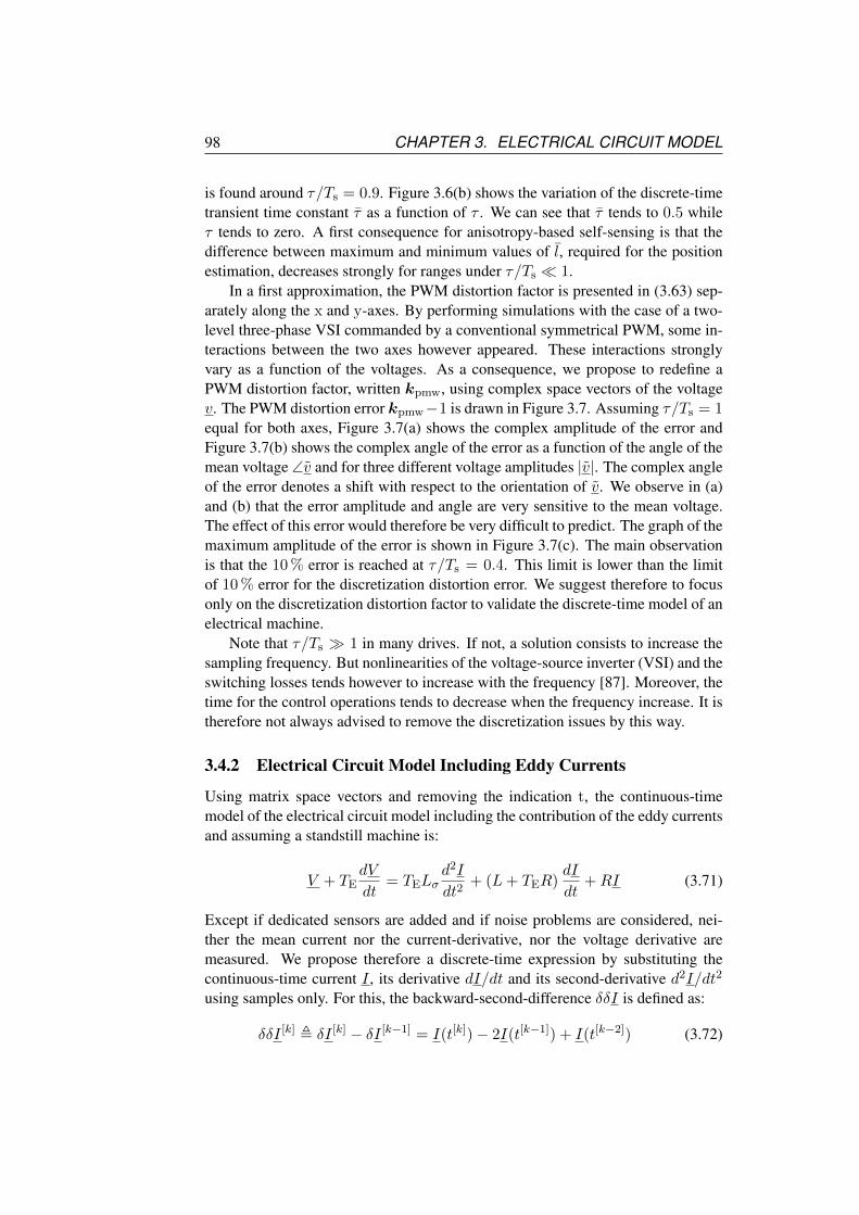
98 CHAPTER 3. ELECTRICAL CIRCUIT MODEL
is found around τ/Ts = 0.9. Figure 3.6(b) shows the variation of the discrete-timetransient time constant τ as a function of τ . We can see that τ tends to 0.5 whileτ tends to zero. A first consequence for anisotropy-based self-sensing is that thedifference between maximum and minimum values of l, required for the positionestimation, decreases strongly for ranges under τ/Ts 1.
In a first approximation, the PWM distortion factor is presented in (3.63) sep-arately along the x and y-axes. By performing simulations with the case of a two-level three-phase VSI commanded by a conventional symmetrical PWM, some in-teractions between the two axes however appeared. These interactions stronglyvary as a function of the voltages. As a consequence, we propose to redefine aPWM distortion factor, written kpmw, using complex space vectors of the voltagev. The PWM distortion error kpmw−1 is drawn in Figure 3.7. Assuming τ/Ts = 1equal for both axes, Figure 3.7(a) shows the complex amplitude of the error andFigure 3.7(b) shows the complex angle of the error as a function of the angle of themean voltage ∠v and for three different voltage amplitudes |v|. The complex angleof the error denotes a shift with respect to the orientation of v. We observe in (a)and (b) that the error amplitude and angle are very sensitive to the mean voltage.The effect of this error would therefore be very difficult to predict. The graph of themaximum amplitude of the error is shown in Figure 3.7(c). The main observationis that the 10 % error is reached at τ/Ts = 0.4. This limit is lower than the limitof 10 % error for the discretization distortion error. We suggest therefore to focusonly on the discretization distortion factor to validate the discrete-time model of anelectrical machine.
Note that τ/Ts 1 in many drives. If not, a solution consists to increase thesampling frequency. But nonlinearities of the voltage-source inverter (VSI) and theswitching losses tends however to increase with the frequency [87]. Moreover, thetime for the control operations tends to decrease when the frequency increase. It istherefore not always advised to remove the discretization issues by this way.
3.4.2 Electrical Circuit Model Including Eddy Currents
Using matrix space vectors and removing the indication t, the continuous-timemodel of the electrical circuit model including the contribution of the eddy currentsand assuming a standstill machine is:
V + TEdV
dt= TELσ
d2I
dt2+ (L+ TER)
dI
dt+RI (3.71)
Except if dedicated sensors are added and if noise problems are considered, nei-ther the mean current nor the current-derivative, nor the voltage derivative aremeasured. We propose therefore a discrete-time expression by substituting thecontinuous-time current I , its derivative dI/dt and its second-derivative d2I/dt2
using samples only. For this, the backward-second-difference δδI is defined as:
δδI [k] , δI [k] − δI [k−1] = I(t[k])− 2I(t[k−1]) + I(t[k−2]) (3.72)
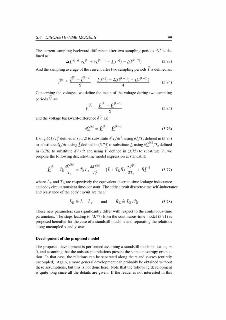
3.4. DISCRETE-TIME MODELS 99
The current sampling backward-difference after two sampling periods ∆I is de-fined as:
∆I [k] , δI [k] + δI [k−1] = I(t[k])− I(t[k−2]) (3.73)
And the sampling average of the current after two sampling periods ¯I is defined as:
¯I[k]
,I
[k]+ I
[k−1]
2=I(t[k]) + 2I(t[k−1]) + I(t[k−2])
4(3.74)
Concerning the voltages, we define the mean of the voltage during two sampling
periods ˜V as: ˜V [k]
=V
[k]+ V
[k−1]
2(3.75)
and the voltage backward-difference δV as:
δV[k]
= V[k] − V [k−1]
(3.76)
Using δδI/T 2s defined in (3.72) to substitute d2I/dt2, using δI/Ts defined in (3.73)
to substitute dI/dt, using ¯I defined in (3.74) to substitute I , using δV[k]/Ts defined
in (3.76) to substitute dV /dt and using ˜V defined in (3.75) to substitute V , wepropose the following discrete-time model expression at standstill:
˜V [k]
+ TEδV
[k]
Ts= TELσ
δδI [k]
T 2s
+(L+ TER
) ∆I[k]
2Ts+ R ¯I
[k](3.77)
where Lσ and TE are respectively the equivalent discrete-time leakage inductanceand eddy circuit transient time-constant. The eddy circuit discrete-time self-inductanceand resistance of the eddy circuit are then:
LE , L− Lσ and RE , LE/TE (3.78)
These new parameters can significantly differ with respect to the continuous-timeparameters. The steps leading to (3.77) from the continuous-time model (3.71) isproposed hereafter for the case of a standstill machine and separating the relationsalong uncoupled x and y-axes.
Development of the proposed model
The proposed development is performed assuming a standstill machine, i.e. ωq =0, and assuming that the anisotropic relations present the same anisotropy orienta-tion. In that case, the relations can be separated along the x and y-axes (entirelyuncoupled). Again, a more general development can probably be obtained withoutthese assumptions, but this is not done here. Note that the following developmentis quite long since all the details are given. If the reader is not interested in this

100 CHAPTER 3. ELECTRICAL CIRCUIT MODEL
long development, we can propose to go to the end of this subsection to read theanalysis.
For convenience, we do not mentioned the axes symbols x and y, but they mustbe considered. For any of the two axes, the components are linked by the followingfirst-order derivative expression:
v(t) + τEdv(t)
dt= τElσ
d2i(t)
dt2+ (l + τEr)
di(t)
dt+ ri(t) (3.79)
where the transient time-constant of the eddy-current circuit is τE = lE/rE. Theglobal behaviour of this model is characterized by two other transient time-constantsτ1 and τ2 than are computed as the inverse and opposite values of the roots x1 andx2 of the following second-order homogeneous equation [86]:
τElσx2 + (l + τEr)x+ r = 0 ⇒ (x− x1)(x− x2) = 0
⇒ τ1 = −1/x1 and τ2 = −1/x2
(3.80)
Note the time-constants can be different along the x-axis and along the y-axis. If τ1
and τ2 are distinct, the solution of this second-order derivative expression betweentwo arbitrary times to and tf is [86]:
i(tf ) = e−tf−toτ1 i1(to) + e
−tf−toτ2 i2(to)
+
∫ tf
to
(v(t)
τE+dv(t)
dt
)(et−tfτ1 − e
t−tfτ2
)dt
/(lστ2− lστ1
)(3.81)
The initial condition is given by:
i(to) = i1(to) + i2(to) (3.82)
The integral right member of (3.81), including the voltage v plus it derivativedv/dt, can be strongly simplified if we assume that the PWM is such that thevoltage is switched to zero at sampling times: v(t[k−1]) = v(t[k]) = 0. This islargely the case in many PWM strategies, such as in the illustration Figure 3.5.Therefore, we can write:
dv(t) et/τ
dt=dv(t)
dtet/τ +
v(t)
τet/τ ∀τ
Since:∫ t[k]
t[k−1]
d(v(t) et/τ
)=(v(t) et/τ
)t[k]
t[k−1]= 0
⇒∫ t[k]
t[k−1]
dv(t)
dtet/τdt = −
∫ t[k]
t[k−1]
v(t)
τet/τdt (3.83)
Introducing (3.83) in (3.81), the integral right member becomes:∫ tf
to
v(t)
et−tfτ1
τE− e
t−tfτ2
τE
−e
t−tfτ1
τ1− e
t−tfτ2
τ2
dt
/(lστ2− lστ1
)(3.84)

3.4. DISCRETE-TIME MODELS 101
This can be further simplified considering the following developments. In onehand, the numerator of (3.84) yields:e
t−tfτ1
τE− e
t−tfτ2
τE
−e
t−tfτ1
τ1− e
t−tfτ2
τ2
=
(1
τE− 1
τ1
)et−tfτ1 −
(1
τE− 1
τ2
)et−tfτ2
= (τ1 − τE)et−tfτ1
τEτ1− (τ2 − τE)
et−tfτ2
τEτ2(3.85)
And in the other hand, the denominator of (3.84) yields:(lστ2− lστ1
)= lσ
τ1 − τ2
τ1τ2(3.86)
From these results, we define two new time-constants:
τ ′1 =lστE
rτ2
(τ1 − τ2
τ1 − τE
)and τ ′2 =
lστE
rτ1
(τ2 − τ1
τ2 − τE
)(3.87)
Introducing (3.87) in (3.84), (3.81) finally yields:
i(tf ) = e−tf−toτ1 i1(to) + e
−tf−toτ2 i2(to)−
1
r
∫ tf
to
v
et−tfτ1
τ ′1+
et−tfτ2
τ ′2
dt (3.88)
In order to obtain a discrete-time model expression, it is required to solve the dif-ferential expression (3.88) during two different periods. As detailed hereafter, wepropose to solve it between:
1. t[k−2] and t[k−1]. It is then possible to remove i1(t[k−2]) and i2(t[k−2]) ;
2. t[k−2] and t[k]. It yields then an expression linking i(t[k]), i(t[k−1]) andi(t[k−2]).
We temporary write the integral right member of (3.88): w1/r between t[k−2] andt[k−1]; and: w2/r between t[k−2] and t[k]. These integrals are further solved. In amatrix form, the initial condition and the solution 1) gathered yield:(
i(t[k−1])− w1/r
i(t[k−2])
)=
(e−Tsτ1 e
−Tsτ2
1 1
)(i1(t[k−2])
i2(t[k−2])
)(3.89)
By inverting it, it yields:
(i1(t[k−2])
i2(t[k−2])
)=
(1 −e
−Tsτ2
−1 e−Tsτ1
)e−Tsτ1 − e
−Tsτ2
(i(t[k−1])− w1/r
i(t[k−2])
)(3.90)

102 CHAPTER 3. ELECTRICAL CIRCUIT MODEL
We have here the relation between i1(t[k−2]) and i2(t[k−2]) and the samples i(t[k−1])and i(t[k−2]). This result can be replaced in the following solution of 2):
i(t[k])−(
e− 2Tsτ1 e
− 2Tsτ2
)( i1(t[k−2])
i2(t[k−2])
)= w2/r (3.91)
The resulting matrix yields:
(e− 2Tsτ1 e
− 2Tsτ2
)(
1 −e−Tsτ2
−1 e−Tsτ1
)e−Tsτ1 − e
−Tsτ2
=
(
e− 2Tsτ1 − e
− 2Tsτ2
)(
e− 2Tsτ2−Tsτ1 − e
− 2Tsτ1−Tsτ2
)t
e−Tsτ1 − e
−Tsτ2
=
(
e−Tsτ1 + e
−Tsτ2
)
−e−(Tsτ2
+Tsτ1
)
t
(3.92)
Combining these results, it yields in a matrix form:
1
−(
e−Tsτ1 + e
−Tsτ2
)
e−(Tsτ2
+Tsτ1
)
t
i(t[k])
i(t[k−1])
i(t[k−2])
= w2/r −(
e−Tsτ1 + e
−Tsτ2
)w1/r (3.93)
The result in an one-line relation is:
i(t[k])−(
e−Tsτ1 + e
−Tsτ2
)i(t[k−1])
+ e−(Tsτ2
+Tsτ1
)i(t[k−2]) = w2/r −
(e−Tsτ1 + e
−Tsτ2
)w1/r (3.94)
We should replace the current samples by the substitution values δδi, ∆i and ¯iusing their definitions (3.72), (3.73) and (3.74). In a matrix form, the definitionsyield: δδi[k]
∆i[k]
¯i[k]
=
1 −2 11 0 −1
0.25 0.5 0.25
i(t[k])
i(t[k−1])
i(t[k−2])
(3.95)

3.4. DISCRETE-TIME MODELS 103
By inverting it, it yields: i(t[k])
i(t[k−1])
i(t[k−2])
=
0.25 0.5 1−0.25 0 10.25 −0.5 1
δδi[k]
∆i[k]
¯i[k]
(3.96)
We have here the relation between the samples and the substitution values. Thisresult can be replaced in the solution (3.93). The resulting matrix yields:
1
−(
e−Tsτ1 + e
−Tsτ2
)
e−(Tsτ2
+Tsτ1
)
t
0.25 0.5 1−0.25 0 10.25 −0.5 1
=
(1 +
(e−Tsτ1 + e
−Tsτ2
)+ e−(Tsτ2
+Tsτ1
))/4(
1− e−(Tsτ2
+Tsτ1
))/2
1−(
e−Tsτ1 + e
−Tsτ2
)+ e−(Tsτ2
+Tsτ1
)
t
=
(1 + e
−Tsτ1
)(1 + e
−Tsτ2
)/4(
1− e−(Tsτ2
+Tsτ1
))/2(
1− e−Tsτ1
)(1− e
−Tsτ2
)
t
(3.97)
Dividing the result by(
1− e−Tsτ1
)(1− e
−Tsτ2
), it yields in an one-line relation:
(1 + e
−Tsτ1
)(1 + e
−Tsτ2
)(
1− e−Tsτ1
)(1− e
−Tsτ2
) δδi[k]
4+
(1− e
−(Tsτ2
+Tsτ1
))(
1− e−Tsτ1
)(1− e
−Tsτ2
)∆i[k]
2+ ¯i
[k]
=
w2/r −(
e−Tsτ1 + e
−Tsτ2
)w1/r(
1− e−Tsτ1
)(1− e
−Tsτ2
) (3.98)
We define here the following discretization distortion factors:
Kδδc2d ,
T 2s
4τ1τ2
(1 + e
−Tsτ1
)(1 + e
−Tsτ2
)(
1− e−Tsτ1
)(1− e
−Tsτ2
) (3.99)

104 CHAPTER 3. ELECTRICAL CIRCUIT MODEL
and
K∆c2d ,
Ts
τ1 + τ2
1− e−Tsτ1−Tsτ2(
1− e−Tsτ1
)(1− e
−Tsτ2
) (3.100)
It can be checked that τ1τ2 = τElσ/r and τ1 +τ2 = τ +τE. Therefore, introducing(3.99) and (3.100) in (3.98) yields:
Kδδc2dτElσ
δδi[k]
T 2s
+K∆c2d (l + τEr)
∆i[k]
2Ts+ r¯i
[k]
=
w2 −(
e−Tsτ1 + e
−Tsτ2
)w1(
1− e−Tsτ1
)(1− e
−Tsτ2
) (3.101)
For the development of the integral right member of (3.101), we separate the inte-gral of w2 between the two sampling periods:
w2 =
∫ t[k]
t[k−2]
v(t)
(et−t[k]
τ1
τ ′1+
et−t[k]
τ2
τ ′2
)dt
=
∫ t[k]
t[k−1]
v(t)
(et−t[k]
τ1
τ ′1+
et−t[k]
τ2
τ ′2
)dt
+
∫ t[k−1]
t[k−2]
v(t)
(et−t[k−1]
τ1
τ ′1e−Tsτ1 +
et−t[k−1]
τ2
τ ′2e−Tsτ2
)dt (3.102)
Gathering the common sampling periods of the integrals, it yields:
w2 −(
e−Tsτ1 + e
−Tsτ2
)w1 =
∫ t[k]
t[k−1]
v(t)
(et−t[k]
τ1
τ ′1+
et−t[k]
τ2
τ ′2
)dt
+
∫ t[k−1]
t[k−2]
v(t)
(et−t[k−1]
τ1
τ ′1e−Tsτ1 +
et−t[k−1]
τ2
τ ′2e−Tsτ2
)dt
−(
e−Tsτ1 + e
−Tsτ2
)∫ t[k−1]
t[k−2]
v(t)
(et−t[k−1]
τ1
τ ′1+
et−t[k−1]
τ2
τ ′2
)dt (3.103)
=
∫ t[k]
t[k−1]
v(t)
(et−t[k]
τ1
τ ′1+
et−t[k]
τ2
τ ′2
)dt
−∫ t[k−1]
t[k−2]
v(t)
(et−t[k−1]
τ1
τ ′1e−Tsτ2 +
et−t[k−1]
τ2
τ ′2e−Tsτ1
)dt (3.104)

3.4. DISCRETE-TIME MODELS 105
=1
τ ′1
(∫ t[k]
t[k−1]
v(t) et−t[k]
τ1 dt−∫ t[k−1]
t[k−2]
v(t) et−t[k]
τ1 e−Tsτ2 dt
)
+1
τ ′2
(∫ t[k]
t[k−1]
v(t) et−t[k]
τ2 dt−∫ t[k−1]
t[k−2]
v(t) et−t[k]
τ2 e−Tsτ1 dt
)(3.105)
We use here the following PWM distortion factors similarly to (3.63) :
k1 [k]pwm ,
∫ t[k]
t[k−1]
v(t)
τ1et−t[k]
τ1 dt
/(v[k]
(1− e
−Tsτ1
))(3.106)
k2 [k]pwm ,
∫ t[k]
t[k−1]
v(t)
τ2et−t[k]
τ2 dt
/(v[k]
(1− e
−Tsτ2
))(3.107)
Using these factors, it yields:
w2 −(
e−Tsτ1 + e
−Tsτ2
)w1
=τ1
τ ′1
(1− e
−Tsτ1
)(k1 [k]
pwmv[k] − k1 [k−1]
pwm v[k−1]e−Tsτ2
)+τ2
τ ′2
(1− e
−Tsτ2
)(k2 [k]
pwmv[k] − k2 [k−1]
pwm v[k−1]e−Tsτ1
)(3.108)
Or, in a matrix form:
=
τ1τ ′1
(1− e
−Tsτ1
)k
1 [k]pwm
+ τ2τ ′2
(1− e
−Tsτ2
)k
2 [k]pwm
− τ1τ ′1
(1− e
−Tsτ1
)k
1 [k−1]pwm e
−Tsτ2
− τ2τ ′2
(1− e
−Tsτ2
)k
2 [k−1]pwm e
−Tsτ1
t
(v[k]
v[k−1]
)(3.109)
We can replace the voltages by the substitution values ˜v and δv using the definitions(3.75) and (3.76). In matrix form, the definitions are:(
˜v[k]
δv[k]
)=
(0.5 0.51 −1
)(v[k]
v[k−1]
)(3.110)
By inverting it, it yields:(v[k]
v[k−1]
)=
(1 0.51 −0.5
)(˜v
[k]
δv[k]
)(3.111)

106 CHAPTER 3. ELECTRICAL CIRCUIT MODEL
This result can be replaced in the solution (3.109). The resulting matrix yields:
τ1τ ′1
(1− e
−Tsτ1
)k
1 [k]pwm
+ τ2τ ′2
(1− e
−Tsτ2
)k
2 [k]pwm
− τ1τ ′1
(1− e
−Tsτ1
)k
1 [k−1]pwm e
−Tsτ2
− τ2τ ′2
(1− e
−Tsτ2
)k
2 [k−1]pwm e
−Tsτ1
t
(1 0.51 −0.5
)
=
τ1τ ′1
(1− e
−Tsτ1
)(k
1 [k]pwm − k1 [k−1]
pwm e−Tsτ2
)+ τ2τ ′2
(1− e
−Tsτ2
)(k
2 [k]pwm − k2 [k−1]
pwm e−Tsτ1
)τ1τ ′1
(1− e
−Tsτ1
)(k
1 [k]pwm + k
1 [k−1]pwm e
−Tsτ2
)/2
+ τ2τ ′2
(1− e
−Tsτ2
)(k
2 [k]pwm + k
2 [k−1]pwm e
−Tsτ1
)/2
t
(3.112)
Note that:
τ1
τ ′1=rτ1τ2
lστE︸ ︷︷ ︸=1
(τ1 − τE
τ1 − τ2
)and
τ2
τ ′2=rτ1τ2
lστE︸ ︷︷ ︸=1
(τ2 − τE
τ2 − τ1
)(3.113)
Introducing these results, (3.109) yields:
v2 −(
e−Tsτ1 + e
−Tsτ2
)v1(
1− e−Tsτ1
)(1− e
−Tsτ2
)
=
(τ1−τEτ1−τ2
)k
1 [k]pwm−k
1 [k−1]pwm e
−Tsτ2
1−e−Tsτ2
+(τ2−τEτ2−τ1
)k
2 [k]pwm−k
2 [k−1]pwm e
−Tsτ1
1−e−Tsτ1
(τ1−τEτ1−τ2
)k
1 [k]pwm+k
1 [k−1]pwm e
−Tsτ2
1−e−Tsτ2
/2
+(τ2−τEτ2−τ1
)k
2 [k]pwm+k
2 [k−1]pwm e
−Tsτ1
1−e−Tsτ1
/2
t
(˜v
[k]
δv[k]
)(3.114)

3.4. DISCRETE-TIME MODELS 107
We define here one new discretization distortion factor and two new PWM distor-tion factors as follows:
k∼ [k]pwm ,
(τ1 − τE
τ1 − τ2
)k
1 [k]pwm − k1 [k−1]
pwm e−Tsτ2
1− e−Tsτ2
+
(τ2 − τE
τ2 − τ1
)k
2 [k]pwm − k2 [k−1]
pwm e−Tsτ1
1− e−Tsτ1
(3.115)
Kδc2d ,
Ts
2τE
((τ1 − τE
τ1 − τ2
)1 + e
−Tsτ2
1− e−Tsτ2
+
(τ2 − τE
τ2 − τ1
)1 + e
−Tsτ1
1− e−Tsτ1
)(3.116)
kδ [k]pwm ,
Ts
2τE
((τ1 − τE
τ1 − τ2
)k
1 [k]pwm + k
1 [k−1]pwm e
−Tsτ2
1− e−Tsτ2
+
(τ2 − τE
τ2 − τ1
)k
2 [k]pwm + k
2 [k−1]pwm e
−Tsτ1
1− e−Tsτ1
)/Kδ
c2d (3.117)
Introducing these factors in (3.109) and replacing the integral right member of(3.101) by the result, it yields the discrete-time model expression:
Kδδc2dτElσ
δδi[k]
T 2s
+K∆c2d (l + τEr)
∆i[k]
2Ts+ r¯i
[k]
= k∼ [k]pwm
˜v[k]+Kδ
c2dkδ [k]pwmτE
δv[k]
Ts(3.118)
Let us define the equivalent discrete-time parameters as follows:
τ[k]E , τE K
δc2dk
δ [k]pwm/k
∼ [k]pwm
r[k] , r/k∼ [k]pwm
l[k]σ , lσ K
δδc2d/K
δc2d/k
δ [k]pwm
l[k] , (l + τEr)K∆c2d/k
∼ [k]pwm − τ [k]
E r[k]
(3.119)
Assume that the PWM distortion error is small, i.e. kδpwm ≈ 1 and k∼pwm ≈ 1,∀k. By consequence, the discrete-time parameters (3.119) are assumed constantand the index [k] can be removed. Introducing them in (3.118) yields the followingdiscrete-time model:
˜v[k]+ τE
δv[k]
Ts= τE lσ
δδi[k]
T 2s
+(l + τE r
) ∆i[k]
2Ts+ r¯i
[k](3.120)
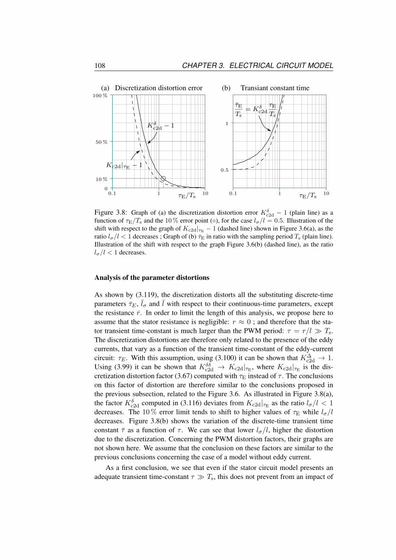
108 CHAPTER 3. ELECTRICAL CIRCUIT MODEL
Discretization distortion error(a) Transiant constant time(b)
00.1
50 %
1 τE/Ts
Kδc2d − 1
Kc2d|τE − 1
100 %
10 %
10τE/Ts0.1
0.5
1
110
τE
Ts= Kδ
c2d
τE
Ts
Figure 3.8: Graph of (a) the discretization distortion error Kδc2d − 1 (plain line) as a
function of τE/Ts and the 10 % error point (), for the case lσ/l = 0.5. Illustration of theshift with respect to the graph of Kc2d|τE − 1 (dashed line) shown in Figure 3.6(a), as theratio lσ/l < 1 decreases ; Graph of (b) τE in ratio with the sampling period Ts (plain line).Illustration of the shift with respect to the graph Figure 3.6(b) (dashed line), as the ratiolσ/l < 1 decreases.
Analysis of the parameter distortions
As shown by (3.119), the discretization distorts all the substituting discrete-timeparameters τE , lσ and l with respect to their continuous-time parameters, exceptthe resistance r. In order to limit the length of this analysis, we propose here toassume that the stator resistance is negligible: r ≈ 0 ; and therefore that the sta-tor transient time-constant is much larger than the PWM period: τ = r/l Ts.The discretization distortions are therefore only related to the presence of the eddycurrents, that vary as a function of the transient time-constant of the eddy-currentcircuit: τE . With this assumption, using (3.100) it can be shown that K∆
c2d → 1.Using (3.99) it can be shown that Kδδ
c2d → Kc2d|τE , where Kc2d|τE is the dis-cretization distortion factor (3.67) computed with τE instead of τ . The conclusionson this factor of distortion are therefore similar to the conclusions proposed inthe previous subsection, related to the Figure 3.6. As illustrated in Figure 3.8(a),the factor Kδ
c2d computed in (3.116) deviates from Kc2d|τE as the ratio lσ/l < 1decreases. The 10 % error limit tends to shift to higher values of τE while lσ/ldecreases. Figure 3.8(b) shows the variation of the discrete-time transient timeconstant τ as a function of τ . We can see that lower lσ/l, higher the distortiondue to the discretization. Concerning the PWM distortion factors, their graphs arenot shown here. We assume that the conclusion on these factors are similar to theprevious conclusions concerning the case of a model without eddy current.
As a first conclusion, we see that even if the stator circuit model presents anadequate transient time-constant τ Ts, this does not prevent from an impact of

3.5. MACHINE IMPEDANCE 109
eddy currents on the discretization. This impact is analyzed hereafter, focusing onsignal-injection-based self-sensing methods. Note also that many models includingthe eddy currents assume a large value of rE. This assumption however lead tohigh values of τE and the discretization impact is therefore augmented. This isnot necessarily a big issue, but this should however be considered to validate themodel.
3.5 Machine Impedance
Many anisotropy-based self-sensing methods using high-frequency signal-injectionsare based on the identification of the high-frequency admittance linking the high-frequency test voltage to the high-frequency current response, and written y(ω). Ifthe admittance contains an anisotropy linked to the rotor, it can be used to trackthe rotor position. In a machine model where the eddy currents are neglected, theimpedance z(ω), that is the inverse of the admittance y(ω) = 1/z(ω), is easilyhandled as the sum of the stator resistance, r, and the incremental self-inductancemultiplied by the frequency of the signals, jωl. In case of significant eddy cur-rents, this model is not valid anymore. Nevertheless, many authors propose to keepthat model and to transpose the impact of the eddy currents on variations of r andl. These parameters becomes then frequency-dependent. They are sometimes re-ferred to as “frequency-dependent”, “apparent”, “eddy-currents-reflected” or sim-ply “high-frequency” [88, 89, 90, 82, 91, 85]. We chose to keep the denomination“apparent” parameters. Signal-injection based self-sensing methods generally relyon the apparent incremental self-inductance.
In this section, we propose the expression of these apparent parameters con-sidering the impact of the eddy-currents, but also the impact of the discretization.For this, we use the discretized models (3.120) and (3.70) that were developedin the previous assuming a standstill machine and assuming anisotropic relationspresenting equal anisotropy orientations, such that the relations can be separatedalong the x and y-axes (entirely uncoupled). A more general model can probablybe proposed without these assumptions, but this is not done here. The different dis-tortion on these apparent parameters are analyzed. Finally, comparisons betweensimulations and experiments validate the models.
For convenience, the upper index [k] referring to the PWM/sampling periodwill not be mentioned on the symbols in the text if it is not confusing. We as-sume that the current variations related to the signal injection are small enough inorder to use the incremental models. For convenience also, the subscript t indi-cating incremental parameters is removed, but all the parameters are necessarilyincremental.

110 CHAPTER 3. ELECTRICAL CIRCUIT MODEL
3.5.1 Continuous-time parameters
In order to allow a comparison, we propose here to introduce the apparent param-eters for the continuous-time case. The model of the standstill machine, along anyof the xy-axes, neglecting the eddy currents is:
v(t) = ldi(t)
dt+ ri(t) (3.121)
The impedance z(ω) is defined as the frequency response of the circuit, com-puted as the transmittance linking the Fourier-transform of the current Fi tothe Fourier-transform of the voltage Fv [46]. It is found using the followingproperty:
Fdx/dt = jωFx x ∈ v, i (3.122)
And yields:z(ω) , Fv/Fi = jωl + r (3.123)
where ω is the considered signal frequency. Including the eddy currents, the modelis:
v(t) + τEdv(t)
dt= τElσ
d2i(t)
dt2+ (l + τEr)
di(t)
dt+ ri(t) (3.124)
The impedance z(ω) then yields:
z(ω) =jω (l + τEr) + r − ω2τElσ
1 + jωτE(3.125)
Using lσ = l − lE, this impedance can be rearranged as follows:
z(ω) =jω (l + τEr) + r − ω2τElσ
1 + ω2τ2E
(1− jωτE)
=jω (l + τEr) + r − ω2τElσ + ω2τE (l + τEr)− jωτE(r − ω2τElσ)
1 + ω2τ2E
=jω(l + ω2τ2
Elσ)
1 + ω2τ2E
+(1 + ω2τ2
E)r + ω2τE(l − lσ)
1 + ω2τ2E
= jω
(l − lE
ω2τ2E
1 + ω2τ2E
)︸ ︷︷ ︸
l(ω)
+
(r + rE
ω2τ2E
1 + ω2τ2E
)︸ ︷︷ ︸
r(ω)
(3.126)
We highlighted here the apparent resistance r(ω) and the apparent incrementalself-inductance l(ω). As we can see, they are frequency-dependent.
Analysis of the apparent values
Including eddy currents, the apparent resistance and incremental self-inductanceof the continuous-time operations are illustrated in Figure 3.9. We see that r varies
3.5. MACHINE IMPEDANCE 111
Apparent inductance l (H)C
ontin
uous
-tim
eApparent resistance r (Ω)
signal frequency ν (logHz)
(II)(III)
(I)
l
lσ
signal frequency ν (logHz)
(II) (III)(I)
r
r + rE
Figure 3.9: Illustration of the apparent parameter values of the continuous-time modelincluding eddy currents, as a function of the frequency ν = ω/(2π). Graphs for cases:τE,(I) > τE,(II) > τE,(III).
between r at low frequencies and r + rE at higher frequencies ; and that l variesbetween l at low frequencies and lσ = l− lE at higher frequencies. The frequencyrange where the apparent parameters shift between the two extrema values dependson the eddy circuit transient time-constant τE. Higher τE, lower is the frequencyof the shift. This is illustrated with cases (I), (II) and (III). This property is usedin some self-sensing strategies where a dedicated closed coil is added at the rotorside [68, 68]. This coil can be handled using the same model as the eddy currentcircuit. It is added along the d or the q-axis in order to modify the anisotropy athigher frequency without affecting the lower-frequency behaviour of the model.
3.5.2 Discrete-time parameters
The discrete-time model of the standstill machine, along any of the xy-axes, ne-glecting the eddy currents is:
v[k] = lδi[k]
Ts+ ri[k] (3.127)
The transmittance linking the Discrete-time Fourier-transform (DTFT) of two val-ues is found using the following property [46]:
Fx[k+1] = ejωTsFx[k] for x[k] ∈ v[k], i(t[k]), i[k], δi[k], . . . (3.128)
Thanks to this property, we can compute the relation between the DTFT of theaverage current i and the sampling backward-difference δi:
Fi(t[k]) = ejωTsFi(t[k−1]) ⇒ Fδi =2(1− e−jωTs
)1 + e−jωTs
Fi (3.129)
This relation can be rearranged in order to define the discrete-time frequency ω:
2(1− e−jωTs
)1 + e−jωTs
=2(ejωTs/2 − e−jωTs/2
)ejωTs/2 + e−jωTs/2
= j2
Tstan(ω
Ts
2)︸ ︷︷ ︸
ω
Ts (3.130)

112 CHAPTER 3. ELECTRICAL CIRCUIT MODEL
Such that δi/Ts = jωi. Let us define ωs = 2π/Ts. Note that ω → ω whenω ωs. Using this result in (3.127) yields the impedance z(ω):
z(ω) , Fv/Fi = jωl + r (3.131)
This expression is quite similar to the continuous-time impedance (3.125). Includ-ing the eddy currents, the model is:
˜v[k]+ τE
δv[k]
Ts= τE lσ
δδi[k]
T 2s
+(l + τE r
) ∆i[k]
2Ts+ r¯i
[k](3.132)
Thanks to the property (3.128), we can compute the relation between the DTFT ofthe average current on two periods ¯i, the backward-difference after two periods ∆iand the backward-second-difference δδi:
F∆i =4(1− e−2jωTs
)1 + 2e−jωTs + e−2jωTs
Fi = 2jωTs Fi (3.133)
and
Fδδi =4(1− 2e−jωTs + e−2jωTs
)1 + 2e−jωTs + e−2jωTs
Fi = −ω2T 2s Fi (3.134)
We have also the following relation:
Fδv = jωTs F˜v (3.135)
Using these relations, the impedance z(ω) then yields and expression similar to thecontinuous-time impedance (3.126):
z(ω) = jω
(l − lE
ω2τ2E
1 + ω2τ2E
)︸ ︷︷ ︸
ˆl(ω)
+
(r + rE
ω2τ2E
1 + ω2τ2E
)︸ ︷︷ ︸
ˆr(ω)
(3.136)
where ˆr(ω) and ˆl(ω) are the apparent resistance and incremental self-inductanceof the discrete-time model.
Analysis of the distortions
Consider firstly the case where we neglect the PWM and discretization distortions.The apparent resistance and inductance of the discrete-time operations are illus-trated in Figure 3.10. From (3.130), we deduced that ω → ω when the samplingfrequency is much higher than the signal frequency, i.e. ωTs π. In that case,illustrated by (I) by the plain line, the discrete-time behaviour of the machine issimilar to the continuous-time case Figure 3.9(II). When the sampling frequencyis decreasing however, i.e. ωTs → π, then ω → ∞. Note that ωTs ≯ π since itis not possible to produce an oscillating signal with a frequency higher than half
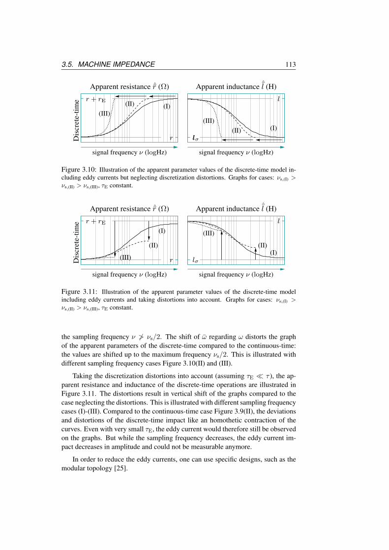
3.5. MACHINE IMPEDANCE 113
Apparent inductance ˆl (H)D
iscr
ete-
time
Apparent resistance ˆr (Ω)
signal frequency ν (logHz)
(III)(I)
lσ
l
(II)
signal frequency ν (logHz)
(III)(I)(II)
r + rE
r
Figure 3.10: Illustration of the apparent parameter values of the discrete-time model in-cluding eddy currents but neglecting discretization distortions. Graphs for cases: νs,(I) >νs,(II) > νs,(III), τE constant.
Apparent inductance ˆl (H)
Dis
cret
e-tim
e
Apparent resistance ˆr (Ω)
signal frequency ν (logHz)
(II)(I)
lσ
l
(III)
signal frequency ν (logHz)
(II)
(I)r + rE
r(III)
Figure 3.11: Illustration of the apparent parameter values of the discrete-time modelincluding eddy currents and taking distortions into account. Graphs for cases: νs,(I) >νs,(II) > νs,(III), τE constant.
the sampling frequency ν ≯ νs/2. The shift of ω regarding ω distorts the graphof the apparent parameters of the discrete-time compared to the continuous-time:the values are shifted up to the maximum frequency νs/2. This is illustrated withdifferent sampling frequency cases Figure 3.10(II) and (III).
Taking the discretization distortions into account (assuming τE τ ), the ap-parent resistance and inductance of the discrete-time operations are illustrated inFigure 3.11. The distortions result in vertical shift of the graphs compared to thecase neglecting the distortions. This is illustrated with different sampling frequencycases (I)-(III). Compared to the continuous-time case Figure 3.9(II), the deviationsand distortions of the discrete-time impact like an homothetic contraction of thecurves. Even with very small τE, the eddy current would therefore still be observedon the graphs. But while the sampling frequency decreases, the eddy current im-pact decreases in amplitude and could not be measurable anymore.
In order to reduce the eddy currents, one can use specific designs, such as themodular topology [25].

114 CHAPTER 3. ELECTRICAL CIRCUIT MODEL
3.5.3 Experiments and Simulations
Experimental set-up
The experiments are performed on the standstill uncoupled experimental BLDCmachine with PM oriented following ϕd = 120, equivalent to ϕq = 30 as il-lustrated in Figure 3.1(a). The PM flux is positive in the negative d-axis direction.The operating stator current io has an amplitude of 25 A and is oriented along thenegative d-axis, i.e. ∠io = −60. This operating stator current is chosen in orderto prevent some effects of the inverter nonlinearities and in order to keep the ro-tor fixed in the desired position. As introduced in chapter 2, with these rotor andcurrent conditions, we have an alignment of the qd frame and the xy frame [92].Therefore: x ≈ q and y ≈ d.
The apparent discrete-time parameters of the experimental machine are iden-tified by the injection of pulsating high-frequency voltages, once along the d-axisand once along the q-axis. More details about the signal injection methods arefound in chapter 5. In order to validate the characteristic curves illustrated in Fig-ure 3.11, the identifications are performed with series of 20 different frequencies ν,that are integer fractions of the PWM frequency: between half the PWM frequencyν = νs/2 down to a fourth of the PWM frequency ν = νs/40. Each series are per-formed for three different PWM frequencies νs at 13 kHz, 10 kHz and 6 kHz. Itwas not possible to reach higher frequencies due to measurement constrains fromthe DSP. In order to assess the standard deviation due to the measurement noise,the computation of each point of the curves is based on 201 samples.
Along the axis νs = 13 kHz 10 kHz 6 kHzx ≈ q 9.6 A 6.0 A 4.8 Ay ≈ d 14.1 A 9.0 A 7.0 A
Table 3.1: Amplitudes of the high-frequency current response |i|.
In order to produce equal high-frequency current amplitudes during every se-ries, the amplitude of the high-frequency voltage is adapted at each frequency ν,from 11.5 V at ν = νs/2 down to 1.8 V at ν = νs/40. Since the results for everyseries were not predictable, the voltage amplitude were not adapted along the twoaxes and for the different PWM frequencies. This choice leads to very differenthigh-frequency current amplitudes, given in Table 3.1. The order of amplitudes(between 3.6 % and 10.5 % of the rated current) was chosen to obtain a satisfyingsignal-to-noise response, especially for the resistance identification.
Measurements compared to simulations
The machine parameters for the simulation have been empirically adjusted in orderto correspond, as good as possible, to the experimental results. By consequence,experiments precede simulations. Parameter estimations are shown in Table 3.2.

3.5. MACHINE IMPEDANCE 115
std/10 std
Apparent inductance ˆl (µH)Apparent resistance ˆr (Ω)
(I)(II)(III)
(I)(II)(III)
103
signal frequency ν (logHz)104102
50
60
70
80
100
90
Nonzero back-emf
Nonzero back-emf
x
y
102 103
0.05
0.10
0.15
104
0.20
Unmodelled phenomenon
x
y
signal frequency ν (logHz)
Figure 3.12: Experimental results of the apparent discrete-time parameter values alongthe x-axis and y-axis. Graphs for cases: νs,(I) = 13 kHz (—), νs,(II) = 10 kHz (- -), νs,(III) =6 kHz (· · · ). The radius of the circles indicate the standard deviation of each point (tenthof it for ˆr).
Apparent inductance ˆl (µH)Apparent resistance ˆr (Ω)
(I)(II)(III)
(I)(II)(III)
103
signal frequency ν (logHz)104102
50
60
70
80
100
90 x
y
signal frequency ν (logHz)102 103
0.05
0.10
0.15
104
0.20
x
y
Figure 3.13: Simulation of the apparent discrete-time parameter values along the x-axisand y-axis assuming continuous-time values given in Table 3.2. Graphs for cases: νs,(I) =13 kHz (—), νs,(II) = 10 kHz (- -), νs,(III) = 6 kHz (· · · ).

116 CHAPTER 3. ELECTRICAL CIRCUIT MODEL
Along the axis r (Ω) l (µH) τ (µs) rE (Ω) lσ (µH) τE (µs)x ≈ q 0.068 95.5 1404 0.5 80 31y ≈ d 0.059 62.5 1059 0.5 51.5 22
Table 3.2: Continuous-time parameters used for the simulations.
Figure 3.12 shows the experimental results with series of identification testsperformed along the x-axis and the y-axis for three different sampling frequencies.Each estimation is computed from 201 samples. The standard deviation (std) isindicated by circles on the graphs. The std is notably larger for ˆr compared to ˆl.Thus the circle radius indicates tenth of the std for ˆr. This difference is explainedby the relative smaller impact of the resistance compared to the inductance, leadingto important noise estimations.
Figure 3.13 shows the simulation results to be compared with Figure 3.12. Thefirst difference concerns the last estimation of ˆr that suddenly deflects downwardly.This is possibly due to missing phenomenon in the modelling such as multipleeddy current sources, skin effects or simply VSI-PWM nonlinearities. The seconddifference concerns the deflection of the estimation of ˆl for lower frequencies. Thisis possibly due to the emergence of undamped high-frequency oscillations and thusto nonzero back-emf. This explanation is evidenced by the higher impact along thex-axis, that is aligned with the torque producing q-axis. Besides these differences,the simulations are consistent with the experiments.
As a conclusion for this experimental machine, the eddy currents produce sig-nificant distortions of the discrete-time parameters, mainly on the apparent resis-tance ˆr that is very sensitive to the signal frequency and to the PWM frequency.These effects should be increased with the rotation speed ωq 6= 0, since angu-lar variations of the inductance appear in the relation (3.59), and that these varia-tions should a fortiori be involved also in the model that includes the eddy currents(3.59). The incremental self-inductance ˆl is also distorted. A large difference of theincremental self-inductance between the two qd axes is however maintained. Asconsequence, this value is still a very good candidate for digital anisotropy-basedself-sensing operations.
3.6 Summary
In this chapter, we introduced the electrical model of the machine using com-plex and matrix space vectors. The issue of cross-saturation, corresponding toanisotropy misalignment, is discussed. The model in the stationary reference-frame, without eddy current, is given in (3.48). This expression involves manyterms:
• the anisotropic incremental relation, that contains the rotor position informa-tion to extract ;

3.6. SUMMARY 117
• the stator resistance that can present anisotropic properties independent tothe rotor position, as shown in shown in (3.29) ;
• terms related to the variation of the inductance ;
• the back-EMF.
Because the control and the self-sensing operations are based on digital mea-surements, a discrete-time model expression is advised. The distortion of thediscrete-time parameters with respect to the continuous-time parameters is mathe-matically studied under the following hypothesis:
• the PWM of the VSI operates on fixed period lengths Ts ;
• the sampling of the measurements is synchronized at the beginning of thePWM periods ;
• we assume a standstill motor for reasons of simplicity in the mathematicaldevelopments ;
• we assume that the model relations can be uncoupled along x and y-axes.
It was possible to distinct two factors of distortion on the parameters:
1. one related to the discretization operation, modelled by the discretizationdistortion factor ;
2. another related to the voltage commutations caused by the PWM, and mod-elled by the PWM distortion factor.
It is firstly shown that the discretization distortion is larger that the PWM distortionfactor, such that we may focus on the discretization distortion only. In case ofnegligible eddy currents, the distortion is function of τ/Ts, where τ = l/r is thetransient time-constant of the stator circuit. Lower this transient time-constant,higher the distortion. It is shown that the discretization distortion reaches 10 % atτ/Ts = 0.9. Fortunately, the stator resistance in many machine is very small andthis condition is satisfied. This is the case of the experimental BLDC motor, whereτy/Ts = 6.35 for the worst studied case at νs = 6 kHz. Noticeable distortionsare however experimentally observed and denotes the presence of significant eddycurrents.
A second mathematical study is thus performed based on an initial continuous-time model including the eddy currents at standstill. Assuming that the transienttime-constant of the stator circuit is much higher than the sampling period τ Ts,the distortion is mainly function of τE/Ts, where τE is the transient time-constantof the eddy-current circuit. Lower this transient time-constant, higher the distor-tion. In the case of the experimental BLDC motor, τE,x/Ts = 0.31 for the beststudied case at νs = 10 kHz. This is very small and it explains why the eddycurrents have a significant impact on the parameter distortions.

118 CHAPTER 3. ELECTRICAL CIRCUIT MODEL
In practice, self-sensing operations identify the machine impedance. This impedanceis generally divided in resistive and inductive contributions. If the eddy currentsare negligible, the resistive contribution is directly related to the stator resistanceand the inductive contribution is related to the incremental self-inductance. If theeddy currents are significant however, many publications on self-sensing methodsstill model the contributions by apparent parameters. These parameters becomefrequency-dependent and are sometimes referred to as eddy-current-reflected.
The strange behaviour of the discretization distortion and the eddy currents aremathematically analyzed. Comparing with simulations, experimental results per-formed on the BLDC motor allow to estimate the motor parameters, including theinaccessible inductance and resistance of the eddy current circuit. These resultsdo not lead to any self-sensing method improvement, but it gives important infor-mation on the machine in order to select the self-sensing method that is the moreadequate.
Note finally that identification methods based on the injection of multi-sine[93] could have been implemented in order to observe the importance of the eddycurrents. However, this type of identification requires additional offset, which wedid not have.

Chapter 4
Voltage-Source Inverter
This chapter addresses the issues of nonlinearities in widespread two-level three-phase voltage source inverters (VSI) commanded by conventional pulsewidth mod-ulated (PWM) signals. Some characteristics of the PWM-VSI leads to nonlinearrelations between the command voltage send to the PWM signal generator and theexpected output voltage. They are mainly due to voltage drops at the semicon-ductors and to commutation delays resulting in so-called dead times. Related tothese nonlinearities, when a phase current crosses zero during the dead times, itis clamped to zero for the rest of that dead time. This phenomenon is referredto as the zero-clamping and has important consequences on the control and onthe self-sensing operations. Solutions to this zero-clamping consist to prevent forzero-crossings, as largely proposed in this chapter.
4.1 Introduction
Many traditional control methods use the command voltage in their models [94],since the nonlinearities generally have limited impacts on the current controller,that compensates for these effects. The self-sensing methods however require anaccurate knowledge of the voltages applied at the machine terminals [95, 96], andthe voltage distortions due to the nonlinearities may have a significant impacts onthe rotor position estimations.
One solution to overcome the nonlinearities consist to introduce voltage sen-sors measuring the mean value of the output voltage during a PWM period, usingdedicated analog [84] or digital integrators [97]. The voltage sensors however re-duce the reliability of the drive (these sensors are additional sources of failure),require data-acquisition hardware [98], result in additional costs and are additionalsource of noise to consider. Another solution consists in the compensation of thenonlinearities. An overview of these nonlinearities and a state-of-the-art of somesolutions to compensate for them are proposed in the first half of the chapter. Wealso introduce the problem of the zero-clamping effect occurring when a phasecurrent crosses zero.
119
120 CHAPTER 4. VOLTAGE-SOURCE INVERTER
This zero-clamping effect is noticeable on the experimental BLDC motor. Itsimpact was so large that the self-sensing methods initially implemented in the ma-chine were inefficient and the position was quickly lost during the rotation. It wastherefore absolutely required to find a method to overcome that problem. Sincethe solutions found in the existing literature were irrelevant for the experimentalconditions, the only solution found was to prevent the zero-crossings of the cur-rent adding an offset to the instruction, with a reduced impact on the torque. Thissolution is addressed in the second half of this chapter
∼
This chapter is organized as follows: the section 4.2 introduces elementarydescriptions of the two-level voltage-source inverter design, the modulation tech-niques and the different nonlinearities, including the zero-clamping phenomenonoccurring when a phase crosses zero ; Section 4.3 describes the zero-crossing is-sue for the point of view of space vectors, and proposes a model of the currentripples that result from the modulation. It also introduces two methods for theestimation of the minimum margin required between the current samples and thezero-crossing lines in order to prevent zero-crossings by the ripples. Finally, itintroduces the operations of the zero-crossing prevention based on the estimatedmargins ; Section 4.4 analyzes the margin estimations for the case of the exper-imental BLDC motor ; A summary of the important elements of this chapter isgiven in section 4.5.
4.2 Pulse-Width Modulated Voltage
This section describes the design of the voltage source inverter (VSI) and its math-ematical model. A VSI provides several outputs with commanded voltages. Thenumber of outputs is related to the number of machine terminals to be connected.The denomination of phase may also refer to the circuits of the VSI for the differentoutputs, but they should not be confused with the machine phases.
We consider a two-level VSI, as it is the most simple and the most widespreadtopology used in industrial power drive applications [99, 18]. In this topology, eachoutput is switched between two voltages, called high or low level voltages, by com-manding the conductivity of two half-bridges. The design of one phase is describedin section 4.2.1. We consider that the half-bridges of every phase are commandedby carrier-based pulsewidth modulated signals [18], also simply called pulsewidthmodulated (PWM) signals, based on cyclical sequences of commutations. A re-view of the state-of-the-art about carrier-based PWM and others such as carrierlessPWM and PWM-control schemes at the year of 1994 is given in [18]. Section 4.2.2addresses the PWM principle, the concept of symmetric and asymmetric modula-tion techniques, and the PWM computation assuming an ideal PWM-VSI. Non-ideal effects of the real VSI (non-ideal) are explained in section 4.2.3, section 4.2.4and section 4.2.4.

4.2. PULSE-WIDTH MODULATED VOLTAGE 121
dc-b
us
vdc2
vdc2
vdc
+ high level
− low level
v+
v−
output
IGBT diode
s?p−
ip
vp
s?p+
brig
debr
igde
+ha
lf-
−ha
lf-
reference potential
Figure 4.1: Design of one phase p of a two-level VSI: a dc-bus with a dc voltage vdc
between a high level (+) and a low level (−); two half-bridges (+) and (−) with free-wheeling devices (diode) and switching devices (IGBT) driven by two switching signalss?p+ and s?p−; an output that presents a voltage vp and delivers a current ip.
4.2.1 The Two-Level Design
The circuit of one phase p of the VSI is shown in Figure 4.1. It is made of twohalf-bridges, one connected to the high level and the other to the low level of thedc-bus, respectively denoted + and −. If the point of the middle voltage of thedc-bus is connected to the ground potential, taken as reference potential, the highand low level voltages are v+ = vdc/2 and v− = −vdc/2 respectively, where vdc
is the dc-bus voltage.
Each half-bridge is composed of two semiconductor devices: one switchingdevice and one freewheeling device (diode). The switching devices are generallyIGBT for medium power applications, and can be MOFSET [100] for lower powerapplications. No snubber circuit coupled to the half-bridges is assumed. A switch-ing signal is sent to the driver of each switching device. The switching signals arenoted s?p+ and s?p− respectively for the high level and low levels of the phase p. Thesignals can take two values 0 or 1. The value 0 denotes a signal that commands thedevice to be in a blocking state and 1 denotes a signal that commands the deviceto be in a conducting state. We say that a signal turns on when it commutates fromblocking 0 to conducting state command 1, and that it turns off when it commutatesfrom conducting 1 to blocking state command 0. The corresponding real switch-ing states of the switching devices are noted sp+ and sp−, for which the value 0denotes a infinite device impedance and 1 denotes a null device impedance. Notethat sp+ = sp− = 1 corresponds to a dc-bus short-circuit and results in a failure.The effective level connection is given by Sp that is 1 if the phase terminal outputis connected to the high level or 0 if it is connected to the low level.
We say that the VSI is ideal if the semiconductor devices are ideal, i.e., theycause no voltage drop and the switching devices commutate instantly between per-fect conducting states and perfect blocking states. In that ideal situation, the output
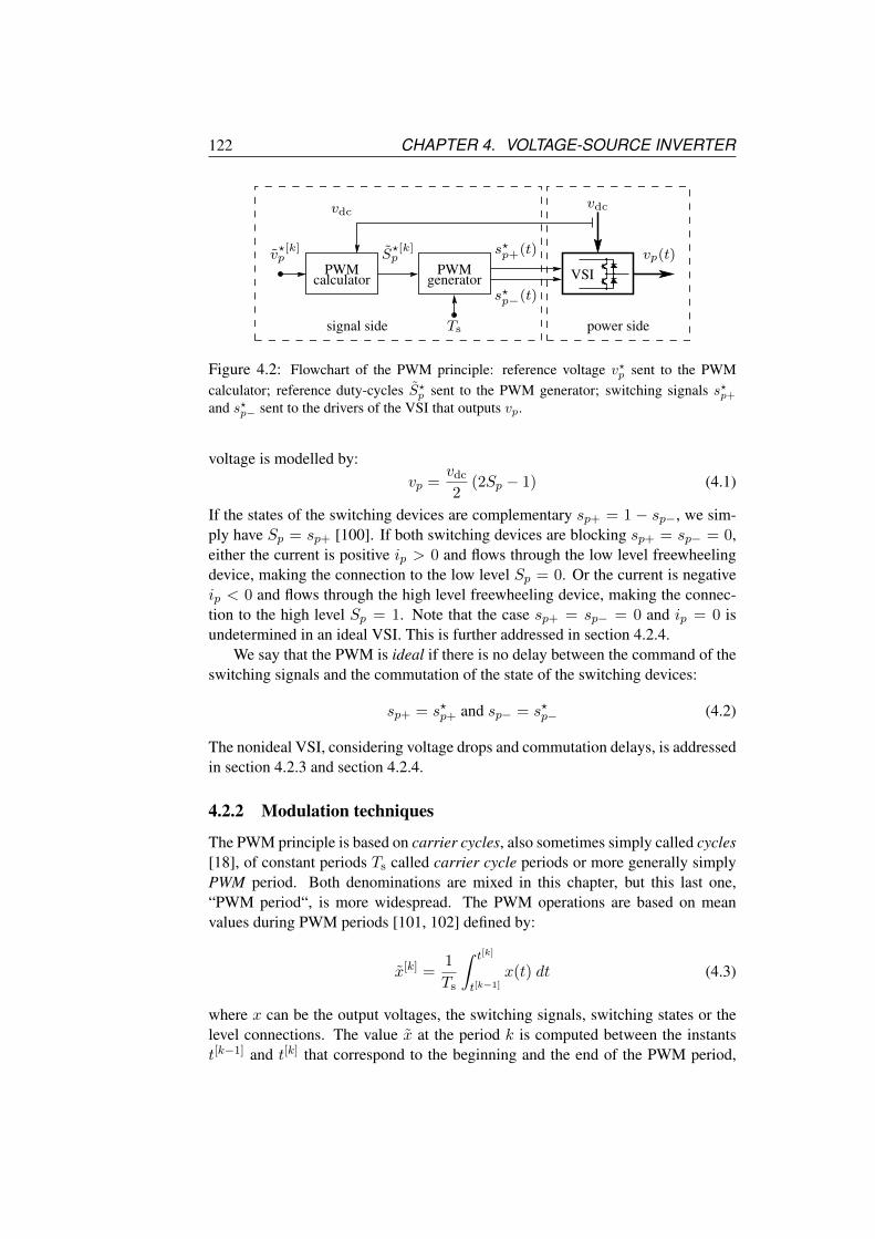
122 CHAPTER 4. VOLTAGE-SOURCE INVERTER
generatorcalculatorPWMPWM
Ts
s?p+(t)
s?p−(t)
signal side
vdc
power side
vdc
vp(t)v?[k]p S
?[k]p
VSI
Figure 4.2: Flowchart of the PWM principle: reference voltage v?p sent to the PWMcalculator; reference duty-cycles S?p sent to the PWM generator; switching signals s?p+and s?p− sent to the drivers of the VSI that outputs vp.
voltage is modelled by:vp =
vdc
2(2Sp − 1) (4.1)
If the states of the switching devices are complementary sp+ = 1 − sp−, we sim-ply have Sp = sp+ [100]. If both switching devices are blocking sp+ = sp− = 0,either the current is positive ip > 0 and flows through the low level freewheelingdevice, making the connection to the low level Sp = 0. Or the current is negativeip < 0 and flows through the high level freewheeling device, making the connec-tion to the high level Sp = 1. Note that the case sp+ = sp− = 0 and ip = 0 isundetermined in an ideal VSI. This is further addressed in section 4.2.4.
We say that the PWM is ideal if there is no delay between the command of theswitching signals and the commutation of the state of the switching devices:
sp+ = s?p+ and sp− = s?p− (4.2)
The nonideal VSI, considering voltage drops and commutation delays, is addressedin section 4.2.3 and section 4.2.4.
4.2.2 Modulation techniques
The PWM principle is based on carrier cycles, also sometimes simply called cycles[18], of constant periods Ts called carrier cycle periods or more generally simplyPWM period. Both denominations are mixed in this chapter, but this last one,“PWM period“, is more widespread. The PWM operations are based on meanvalues during PWM periods [101, 102] defined by:
x[k] =1
Ts
∫ t[k]
t[k−1]
x(t) dt (4.3)
where x can be the output voltages, the switching signals, switching states or thelevel connections. The value x at the period k is computed between the instantst[k−1] and t[k] that correspond to the beginning and the end of the PWM period,
4.2. PULSE-WIDTH MODULATED VOLTAGE 123
such that Ts = t[k]−t[k−1]. We assume that these instants are synchronized with thesampling times of the current measurements sampling, as described in section 3.5.The mean Sp of Sp is the duty-cycle corresponding to the relative duration of thehigh level connection, assuming a low level connection the rest of the PWM period.Note that 0 ≤ Sp ≤ 1. For convenience and in order to shorten the expressions,the upper index [k] mentioning the period is sometimes not mentioned if it is notconfusing.
As explained by a flowchart in Figure 4.2 for one phase p, before each cycle,a reference voltage v?p is sent to a PWM calculator. This calculator computes areference duty-cycle S?p . This reference duty-cycle is sent to a PWM generator thatsynthesizes the two switching signals s?p+ and s?p− [103]. The switching signalsare sent to the drivers of the switching devices of the VSI. Note that no signalcorresponding to S?p is ever computed, as S?p is directly used as a reference valueto synthesize the switching signals s?p+ and s?p−.
The reference duty-cycle S?p is generally computed by the PWM calculator sothat the mean of the output voltage vp is equal to the reference voltage [104, 94]:
vp = v?p (4.4)
If this condition is actually satisfied, the reference voltage v?p can be used insteadof the output voltage in rotation-drive operations, self-sensing operations and anyother operations based on the discrete-time model of the machine, as explained insection 3.5 of chapter 3. The computation leading to (4.4) is explained here below.
Duty-Cycle Computation
Assume that the VSI is ideal (4.1) and that the PWM is also ideal (4.2). If the PWMgenerator synthesizes complementary switching signals s?p+ = 1 − s?p− such thats?p+ = S?p , the mean output voltage defined by (4.3) during every cycle k yields:
vp =vdc
2
(2S?p − 1
)(4.5)
By consequence, in order to have vp = v?p , as given in (4.4), the PWM calculatorshould compute its output using the following expression:
S?p :=v?pvdc
+ 0.5 (4.6)
The nonideal VSI introduce a nonlinear relation between s?p+ and vp. The expres-sion (4.6) must therefore be adapted in order to take the nonlinearity into account,as further explained.
Symmetric and asymmetric modulations
Before introducing the VSI nonlinearities, it is required to shortly explain the prin-ciple of the PWM. The conventional modulation techniques are based on two car-

124 CHAPTER 4. VOLTAGE-SOURCE INVERTER
(b) asymmetric modulation(a) symmetric modulation
vdc2
− vdc2
t[k−1] t[k−12
] t[k] t[k−1] t[k−12
] t[k]
1
0
S?[k]p Ts S
?[k]p Ts
0
1
S?[k]p
Ts2
S?[k]p
Ts2
S?[k],p
Ts2
S?[k],p
Ts2
Ts/2 Ts/2 Ts/2Ts/2
vp(t)v[k] v[k]
ip(t)
s?p−(t)
s?p+(t)
v?p
v?[k]
v?[k]
v?[k]
Figure 4.3: Switching signals s?p± synthesized by the PWM generator, assuming comple-mentary signals: illustration by two carrier half-cycles in case of (a) symmetric modulationand (b) asymmetric modulation, assuming (S?,p + S?,p)/2 = S?p .
rier half-cycles of equal durations Ts/2 (PWM half-periods) [18]. The values cor-responding to the first and the second carrier half-cycles will be denoted respec-tively by the lower index and . Let us therefore define the mean values x andx of the variable x respectively during the first and the second half-cycle periodsas follow:
x[k] =
1
Ts/2
∫ t[k−1/2]
t[k−1]
x(t) dt and x[k] =
1
Ts/2
∫ t[k]
t[k−1/2]
x(t) dt (4.7)
where t[k−1/2] is conventionally the middle instant of the PWM period: t[k−1/2] =(t[k] + t[k−1])/2. Using (4.7), we can define two distinct reference half-duty-cyclesS?,p and S?,p. In the continuous modulation techniques, every switching signals?p± turns “on” or “off” once during the first half-cycle and turns reversely “off”or “on” once during the second half-cycle. Two continuous modulation techniquesare illustrated in Figure 4.3 [18]:
(a) either S?,p and S?,p are equal to S?p and the modulation is said symmetric. Thereference duty-cycle S?p is calculated from one reference voltage v?p using(4.6) ;

4.2. PULSE-WIDTH MODULATED VOLTAGE 125
vscrscisc
uth
0
iscisc,o0
Figure 4.4: Typical voltage/currentcharacteristic of a diode and linearizedmodel.
t[k−1] t[k]
Ts
vdc2
− vdc2
vdc2
− vdc2
vs,p
(b) ip < 0
(a) ip > 0
vp(t)
vp(t)
Figure 4.5: PWM-VSI considering thesemiconductor voltage drops: effect on theoutput voltage vp if (a) ip > 0 (b) ip < 0.
(b) or S?,p and S?,p are different and the modulation is said asymmetric [105], orunsymmetrical [106]. Hence, both S?,p and S?,p can be computed from twodifferent reference voltages v?,p and v?,p using (4.6).
All the PWM generator does not offer the possibility to work in an asymmetricmodulation mode. This is the case of the PWM generator of our test bench thatonly allows symmetric modulations. In practice however, due to inherent delaysof the commutations of the nonideal VSI, the actual half-duty-cycles are alwaysslightly different [107]. This slight difference is considered in the VSI nonlineari-ties addressed hereafter.
Note that many other modulation techniques exist. Among the conventionalmodulation techniques, the discontinuous modulation techniques are characterizedby the saturation of the reference duty-cycle of one phase or more [99, 100]: S?p =
1 or S?p = 0. In that case, no switching may occur in the phase p. Some newer nonconventional modulation techniques such as [108] are characterized by switchingsignals turning on or off more than once during the carrier half-cycles. Intuitively,the method we propose could be extended to these cases, but this document onlyfocuses on the conventional modulation techniques.
4.2.3 Semiconductor Voltage Drop
The first nonlinearity introduced by the real VSI comes from the voltage drops thatexist across the semiconductor devices. For illustration, a typical static voltage/cur-rent characteristic of a diode is presented Figure 4.4. Note that the characteristicsare generally different between the switching and freewheeling device types andvary with the temperature [5]. Let define vsc,p that models an equivalent voltagedrop at the phase output p. The output voltage is
vp|real = vp|ideal − vsc,p(ip, sp+, sp−,T) (4.8)
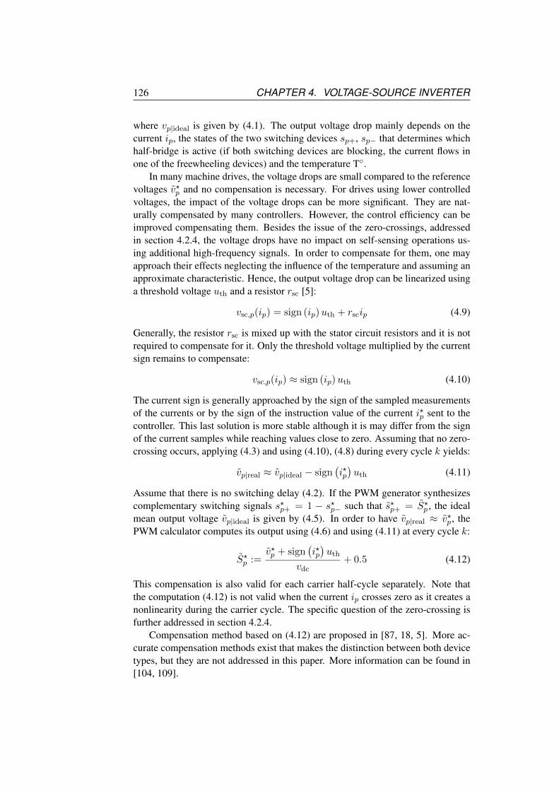
126 CHAPTER 4. VOLTAGE-SOURCE INVERTER
where vp|ideal is given by (4.1). The output voltage drop mainly depends on thecurrent ip, the states of the two switching devices sp+, sp− that determines whichhalf-bridge is active (if both switching devices are blocking, the current flows inone of the freewheeling devices) and the temperature T.
In many machine drives, the voltage drops are small compared to the referencevoltages v?p and no compensation is necessary. For drives using lower controlledvoltages, the impact of the voltage drops can be more significant. They are nat-urally compensated by many controllers. However, the control efficiency can beimproved compensating them. Besides the issue of the zero-crossings, addressedin section 4.2.4, the voltage drops have no impact on self-sensing operations us-ing additional high-frequency signals. In order to compensate for them, one mayapproach their effects neglecting the influence of the temperature and assuming anapproximate characteristic. Hence, the output voltage drop can be linearized usinga threshold voltage uth and a resistor rsc [5]:
vsc,p(ip) = sign (ip)uth + rscip (4.9)
Generally, the resistor rsc is mixed up with the stator circuit resistors and it is notrequired to compensate for it. Only the threshold voltage multiplied by the currentsign remains to compensate:
vsc,p(ip) ≈ sign (ip)uth (4.10)
The current sign is generally approached by the sign of the sampled measurementsof the currents or by the sign of the instruction value of the current i?p sent to thecontroller. This last solution is more stable although it is may differ from the signof the current samples while reaching values close to zero. Assuming that no zero-crossing occurs, applying (4.3) and using (4.10), (4.8) during every cycle k yields:
vp|real ≈ vp|ideal − sign(i?p)uth (4.11)
Assume that there is no switching delay (4.2). If the PWM generator synthesizescomplementary switching signals s?p+ = 1 − s?p− such that s?p+ = S?p , the idealmean output voltage vp|ideal is given by (4.5). In order to have vp|real ≈ v?p , thePWM calculator computes its output using (4.6) and using (4.11) at every cycle k:
S?p :=v?p + sign
(i?p)uth
vdc+ 0.5 (4.12)
This compensation is also valid for each carrier half-cycle separately. Note thatthe computation (4.12) is not valid when the current ip crosses zero as it creates anonlinearity during the carrier cycle. The specific question of the zero-crossing isfurther addressed in section 4.2.4.
Compensation method based on (4.12) are proposed in [87, 18, 5]. More ac-curate compensation methods exist that makes the distinction between both devicetypes, but they are not addressed in this paper. More information can be found in[104, 109].

4.2. PULSE-WIDTH MODULATED VOLTAGE 127
Switching delays in high-level connection
Switching delays in low-level connection
zoom zoom
zoom zoom
∆ton ∆toff∆tlag
∆tlagS?[k],p
Ts2
S?[k],p
Ts2
0
1
0
1
vdc2
− vdc2
∆tdt, ∆tdt,S
[k],p
Ts2
S[k],p
Ts2∆tdt
t[k−1] t[k]t[k−12
]
1
0
S?[k],p
Ts2
S?[k],p
Ts2
Ts/2 Ts/2
1
0
S?[k],p
Ts2
S?[k],p
Ts2
Ts/2 Ts/2
t[k−1] t[k]t[k−12
]
0
1
0
1
∆ton∆tlag∆toff
S?[k],p
Ts2 ∆tlag
S?[k],p
Ts2
vdc2
− vdc2
∆tdt,S
[k],p
Ts2
S[k],p
Ts2
∆tdt∆tdt,
(a) case ip > 0
(b) case ip < 0
⇒
s?p+(t)
sp+(t)
vp(t)
s?p+(t)
s?p−(t)
sp−(t)
s?p−(t)
⇒
vp(t)
Figure 4.6: Zoom in two half-cycles of the PWM-VSI showing the switching delays: ex-pected switching signals (- -) and synthesized switching signals s?p+ and s?p− (—), switch-ing states sp+ and sp− with their commutation delays. Output voltage vp in case (a) ip ispositive and in case (b) ip is negative.
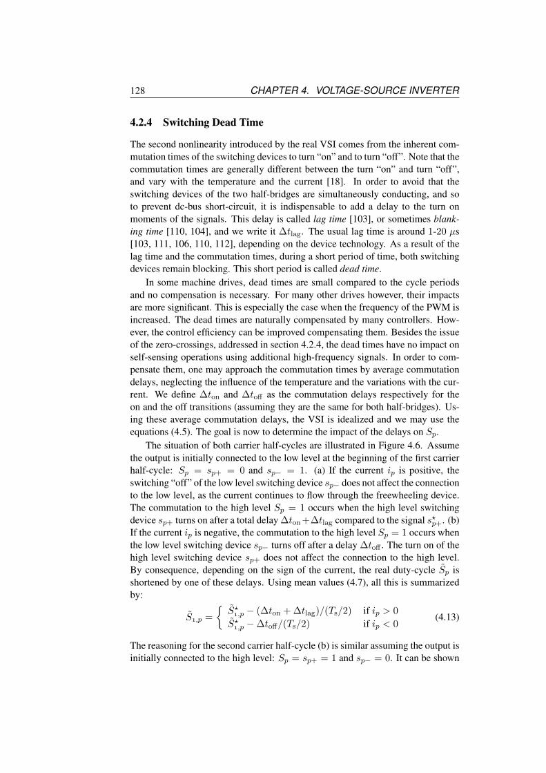
128 CHAPTER 4. VOLTAGE-SOURCE INVERTER
4.2.4 Switching Dead Time
The second nonlinearity introduced by the real VSI comes from the inherent com-mutation times of the switching devices to turn “on” and to turn “off”. Note that thecommutation times are generally different between the turn “on” and turn “off”,and vary with the temperature and the current [18]. In order to avoid that theswitching devices of the two half-bridges are simultaneously conducting, and soto prevent dc-bus short-circuit, it is indispensable to add a delay to the turn onmoments of the signals. This delay is called lag time [103], or sometimes blank-ing time [110, 104], and we write it ∆tlag. The usual lag time is around 1-20 µs[103, 111, 106, 110, 112], depending on the device technology. As a result of thelag time and the commutation times, during a short period of time, both switchingdevices remain blocking. This short period is called dead time.
In some machine drives, dead times are small compared to the cycle periodsand no compensation is necessary. For many other drives however, their impactsare more significant. This is especially the case when the frequency of the PWM isincreased. The dead times are naturally compensated by many controllers. How-ever, the control efficiency can be improved compensating them. Besides the issueof the zero-crossings, addressed in section 4.2.4, the dead times have no impact onself-sensing operations using additional high-frequency signals. In order to com-pensate them, one may approach the commutation times by average commutationdelays, neglecting the influence of the temperature and the variations with the cur-rent. We define ∆ton and ∆toff as the commutation delays respectively for theon and the off transitions (assuming they are the same for both half-bridges). Us-ing these average commutation delays, the VSI is idealized and we may use theequations (4.5). The goal is now to determine the impact of the delays on Sp.
The situation of both carrier half-cycles are illustrated in Figure 4.6. Assumethe output is initially connected to the low level at the beginning of the first carrierhalf-cycle: Sp = sp+ = 0 and sp− = 1. (a) If the current ip is positive, theswitching “off” of the low level switching device sp− does not affect the connectionto the low level, as the current continues to flow through the freewheeling device.The commutation to the high level Sp = 1 occurs when the high level switchingdevice sp+ turns on after a total delay ∆ton +∆tlag compared to the signal s?p+. (b)If the current ip is negative, the commutation to the high level Sp = 1 occurs whenthe low level switching device sp− turns off after a delay ∆toff . The turn on of thehigh level switching device sp+ does not affect the connection to the high level.By consequence, depending on the sign of the current, the real duty-cycle Sp isshortened by one of these delays. Using mean values (4.7), all this is summarizedby:
S,p =
S?,p − (∆ton + ∆tlag)/(Ts/2) if ip > 0
S?,p −∆toff/(Ts/2) if ip < 0(4.13)
The reasoning for the second carrier half-cycle (b) is similar assuming the output isinitially connected to the high level: Sp = sp+ = 1 and sp− = 0. It can be shown

4.2. PULSE-WIDTH MODULATED VOLTAGE 129
that the result is:
S,p =
S?,p + ∆toff/(Ts/2) if ip > 0
S?,p + (∆ton + ∆tlag)/(Ts/2) if ip < 0(4.14)
If we use a symmetric modulation, remember that we have S?,p = S?,p = S?p . Theresulting duty-cycle during Ts is given by:
Sp =S,p + S,p
2= S?p − sign (ip)
∆tdt
Ts(4.15)
where:∆tdt = ∆ton −∆toff + ∆tlag (4.16)
This expression is found in many publications, such as [113, 104]. Remark: the re-lations (4.13) and (4.14) do not model situations where S,p or S,p is smaller than0 or larger than 1, since it would correspond to commutations occurring outside thehalf-cycle.
Assuming that no zero-crossing occurs, the sign of the current is generallyapproached by the sign of the sampled measurements of the currents or by the signof the instruction value of the current i?p sent to the controller. In that last case,(4.15) yields:
Sp ≈ S?p − sign(i?p) ∆tdt
Ts(4.17)
Assume that the VSI is ideal (4.1), i.e. no voltage drop. In order to have vp ≈ v?p ,the computation of the PWM calculator is found using (4.17) and yields:
S?p :=v?pvdc
+ sign(i?p) ∆tdt
Ts+ 0.5 (4.18)
This compensation is no valid for each carrier half-cycle separately. For this, thedistinct expressions (4.13) and (4.14) must be used. Note also that this solutionis not valid when the current ip crosses zero. The specific question of the zero-crossing is addressed hereafter.
Some methods are included in the control operations, such as in [113, 111,5, 112]. The benefit is that the PWM generator is not modified and no additionalsetup is required. Such a method in integrated in an self-sensing control using high-frequency signal injection by [114]. It is also possible to take benefit of asymmetricmodulations in order to specifically compensate the dead times during every half-cycles, as done in [106, 107, 115]. This has the advantage to improve the shapeof the PWM compared to the first methods, an asymmetric PWM generator is re-quired. The solution proposed by [110] is based on the fact that when the currentof a phase is flowing in the diode of a half-bridge, it is not necessary to turn onthe switching device of this half-bridge. By consequence, no lag time delay is re-quired. Older methods use additional analogical delayers, such as [116, 117, 118].They are not much used to our knowledge. All the mentioned methods are based on
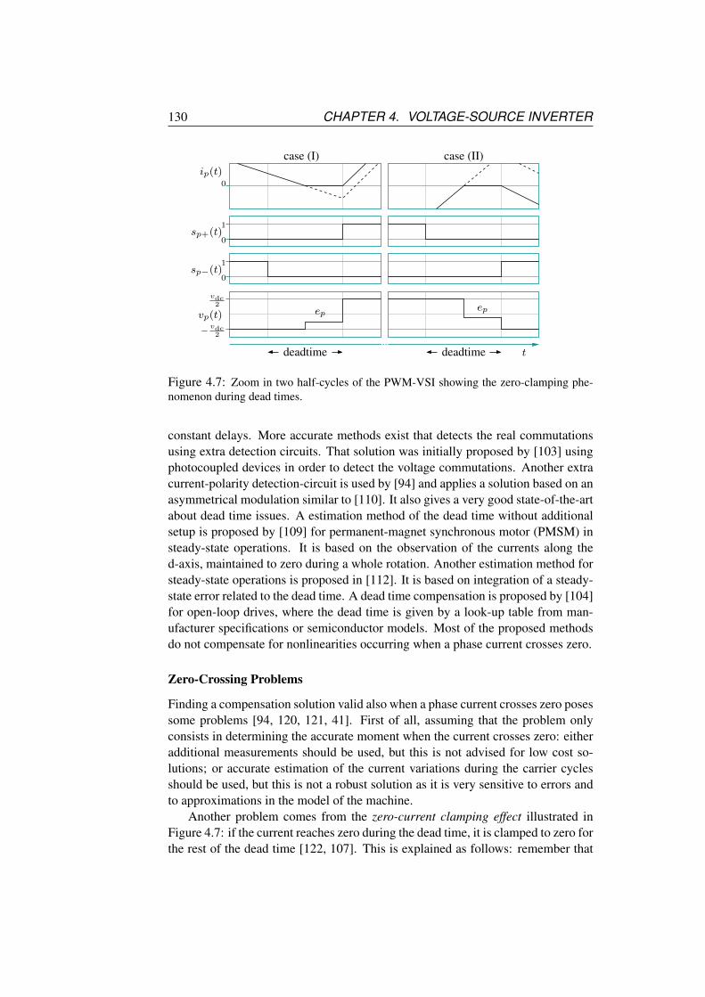
130 CHAPTER 4. VOLTAGE-SOURCE INVERTER
case (I) case (II)
deadtime deadtime
1
0
0
1
0
vdc2
− vdc2
t
ip(t)
vp(t)epep
sp+(t)
sp−(t)
Figure 4.7: Zoom in two half-cycles of the PWM-VSI showing the zero-clamping phe-nomenon during dead times.
constant delays. More accurate methods exist that detects the real commutationsusing extra detection circuits. That solution was initially proposed by [103] usingphotocoupled devices in order to detect the voltage commutations. Another extracurrent-polarity detection-circuit is used by [94] and applies a solution based on anasymmetrical modulation similar to [110]. It also gives a very good state-of-the-artabout dead time issues. A estimation method of the dead time without additionalsetup is proposed by [109] for permanent-magnet synchronous motor (PMSM) insteady-state operations. It is based on the observation of the currents along thed-axis, maintained to zero during a whole rotation. Another estimation method forsteady-state operations is proposed in [112]. It is based on integration of a steady-state error related to the dead time. A dead time compensation is proposed by [104]for open-loop drives, where the dead time is given by a look-up table from man-ufacturer specifications or semiconductor models. Most of the proposed methodsdo not compensate for nonlinearities occurring when a phase current crosses zero.
Zero-Crossing Problems
Finding a compensation solution valid also when a phase current crosses zero posessome problems [94, 120, 121, 41]. First of all, assuming that the problem onlyconsists in determining the accurate moment when the current crosses zero: eitheradditional measurements should be used, but this is not advised for low cost so-lutions; or accurate estimation of the current variations during the carrier cyclesshould be used, but this is not a robust solution as it is very sensitive to errors andto approximations in the model of the machine.
Another problem comes from the zero-current clamping effect illustrated inFigure 4.7: if the current reaches zero during the dead time, it is clamped to zero forthe rest of the dead time [122, 107]. This is explained as follows: remember that

4.3. ZERO-CROSSING ISSUES AND PREVENTION 131
the current flows in one of the freewheeling devices while the switching devicesare blocking. To overpass the voltage drop across the freewheeling device, theoutput voltage vp must necessarily be higher than the high level voltage v+: vp =v+ + vdiode if ip < 0; or lower than the low level voltage v−: vp = v− − vdiode ifip > 0. Note that this is possible because the machine is an inductive circuit. Thefact that ip slides to zero is related to a decrease of vdiode, as shown in Figure 4.4.The freewheeling device becomes blocking when the current reaches zero. Atthis moment, both freewheeling devices are blocking and all the half-bridges arecompletely blocking. As a consequence, the output voltage freely varies betweenthe low level and the high level voltages: v− < vp < v+. This phenomenon isnot easy modelled since it is strongly nonlinear, the zero-clamping instant is verysensitive to very small variations of the current, and the topology of the machine ischanged with one disconnected phase during the zero-clamping.
The solutions proposed by [122, 123] consist in a compensation method basedon the repetitive nature of the zero-crossing in steady-state operations. The so-lution is integrated by [96] in back-EMF-based self-sensing methods. In [107], afeedback term in a predictive current controllers is used in order to reduce the zero-current clamping effect. This effect is however not completely compensated. Allthese solutions are not operating correctly during transient operations and are notefficient for many anisotropy-based self-sensing methods due to the large approx-imation of the correction. An improved method integrated in self-sensing opera-tions is proposed by [124]. The duration of the zero-crossing, to be compensated,is predicted using a first-order approximation of the circuit model. This solutionhowever assume only small ripple amplitudes and the accuracy should be furtheranalyzed with machine presenting significant resistive voltage drops.
If we want to keep a simple hardware solution and a low computation time,one solution is therefore to find a method that maintains ip far enough from zeromost of the time, for example adding an offset in the current reference. When azero-crossing is required, it must occur as quick as possible, for example duringone carrier cycle, in order to reduce its impact. Ideally, the offset is selected inorder to minimize its impact on the torque and the performances of the machine.This is addressed in the next section 4.3.
4.3 Zero-Crossing Issues and Prevention
We restrict the analysis to the case of a three-phase VSI supplying a three-phasemachine without neutral connection, i.e. without homopolar current io = 0. TheVSI phases are numbered by p ∈ a,b, c. The proposed solution is based onspace vectors handled in the stationary αβ reference-frame.
Due to the pulsewidth modulation (PWM) principle of the voltage source in-verters, described in section 4.2.2, the space vector of the output voltage switchesbetween fixed values, called switching-state voltage space-vectors, during the car-rier cycle. These voltages are addressed in section 4.3.1. These switches result in
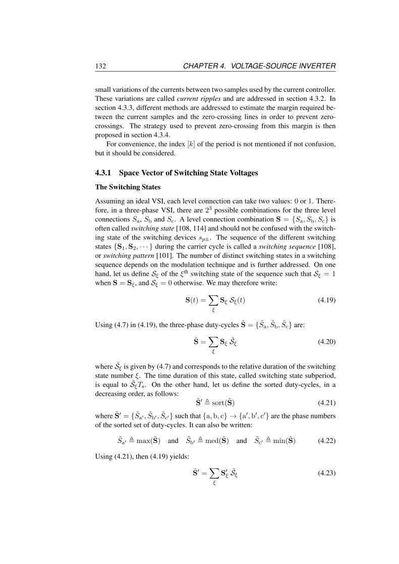
132 CHAPTER 4. VOLTAGE-SOURCE INVERTER
small variations of the currents between two samples used by the current controller.These variations are called current ripples and are addressed in section 4.3.2. Insection 4.3.3, different methods are addressed to estimate the margin required be-tween the current samples and the zero-crossing lines in order to prevent zero-crossings. The strategy used to prevent zero-crossing from this margin is thenproposed in section 4.3.4.
For convenience, the index [k] of the period is not mentioned if not confusion,but it should be considered.
4.3.1 Space Vector of Switching State Voltages
The Switching States
Assuming an ideal VSI, each level connection can take two values: 0 or 1. There-fore, in a three-phase VSI, there are 23 possible combinations for the three levelconnections Sa, Sb and Sc. A level connection combination S = Sa, Sb, Sc isoften called switching state [108, 114] and should not be confused with the switch-ing state of the switching devices sp±. The sequence of the different switchingstates S1,S2, · · · during the carrier cycle is called a switching sequence [108],or switching pattern [101]. The number of distinct switching states in a switchingsequence depends on the modulation technique and is further addressed. On onehand, let us define Sξ of the ξth switching state of the sequence such that Sξ = 1when S = Sξ, and Sξ = 0 otherwise. We may therefore write:
S(t) =∑ξ
Sξ Sξ(t) (4.19)
Using (4.7) in (4.19), the three-phase duty-cycles S = Sa, Sb, Sc are:
S =∑ξ
Sξ Sξ (4.20)
where Sξ is given by (4.7) and corresponds to the relative duration of the switchingstate number ξ. The time duration of this state, called switching state subperiod,is equal to SξTs. On the other hand, let us define the sorted duty-cycles, in adecreasing order, as follows:
S′ , sort(S) (4.21)
where S′ = Sa′ , Sb′ , Sc′ such that a,b, c → a′, b′, c′ are the phase numbersof the sorted set of duty-cycles. It can also be written:
Sa′ , max(S) and Sb′ , med(S) and Sc′ , min(S) (4.22)
Using (4.21), then (4.19) yields:
S′ =∑ξ
S′ξ Sξ (4.23)

4.3. ZERO-CROSSING ISSUES AND PREVENTION 133
Level connections and Switching states
Ts
SaTs = Sb′Ts
SbTs = Sa′Ts
ScTs = Sc′Ts
S1Ts =(
1 − Sa′
)Ts/2
S2Ts =(Sa′ − Sb′
)Ts/2
1
0
1
0
1
0
1
0
0
1
t[k−1] t[k]t[k−12
]
12341 2 3 4
000 010110111 000010110111000 100110111 000100110111
xζ =
S(t) =
S′(t) =
S1(t)
S2(t)
= Sb′ (t)
= Sa′ (t)
= Sc′ (t)Sc(t)
Sb(t)
Sa(t)
Figure 4.8: Illustration of the level connections Sp and their sorted numbering Sp′ inan ideal conventional symmetrical modulation technique commanding an ideal two-levelthree-phase VSI. In this example: a′ = b, b′ = c and c′ = c. Corresponding switchingstates Sxζ and ordered switching states S′xζ numbered from xζ = 1 to 4 for the firsthalf-period and from xζ = 4 to 1 for the second half-period. Illustration of S1(t) andS2(t) (the next Sxζ(t) follow the same principle).
where S′ξ = Sa′ , Sb′ , Sc′ξ. Note that Sξ is not affected by the sorting. Theserelations (4.19)-(4.23) are also valid for carrier half-cycles using (4.7).
As illustrated in Figure 4.8 for a continuous modulation technique, during ev-ery carrier half-cycle, each VSI phase output switches once between the high andlow levels. Therefore, in a three-phase VSI, there are four different switchingstates in one switching half-sequence. By consequence, instead of numbering theswitching states by 1, 2, . . . , let us number them by an index made of the half-cyclenumber x ∈ , followed by their order of occurrence from ξ = 1 to 4 in the firstswitching half-sequence: S1,S2,S3,S4; and reversely from ξ = 4 to 1 inthe second switching half-sequence: S4,S3,S2,S1. Using this numbering, itis possible to write expressions that cover indiscriminately each carrier half-cycle.Note that if the modulation is perfectly symmetric: Sξ = Sξ, ∀ξ ∈ 1, 2, 3, 4.
Assume a continuous modulation technique with Sx1 = 000 and Sx4 =111. Using the sorting of the duty-cycles as defined in (4.21) or (4.22), it can be

134 CHAPTER 4. VOLTAGE-SOURCE INVERTER
shown that the respective consecutive switching states are:
S′x1 = 000S′x2 = 100S′x3 = 110S′x4 = 111
(4.24)
In other words, the different level connections switch “on” successively in the or-der of their sorted duty-cycles. Assuming a symmetric modulation, it can also bedemonstrated that the successive switching state durations are:
Sx1 =(
1 − Sa′
)/2
Sx2 =(Sa′ − Sb′
)/2
Sx3 =(Sb′ − Sc′
)/2
Sx4 =(Sc′
)/2
(4.25)
where a′, b′, c′ are the sorted phase numbers. The same computation is alsovalid for each carrier half-cycles in case of an asymmetric modulation, consideringdistinct half-duty-cycles. Note that, in that asymmetric modulation case, the ordera′,b′, c′ is not necessarily the same for the first and the second carrier half-cycles. As a conclusion, the duration of the different switching states are easilycomputed from the sorted phase duty-cycles. In case of nonideal three-phase VSI,the same computation (4.25) is valid, but the dead times should be cut off the duty-cycle computations, as explained in section 4.2.4.
The Switching-State Voltage Space-Vectors
The space vector v of the output voltage is defined by (2.71) in chapter 2 as thephase contributions vp counted along the conductor orientations ϕp:
v ,2
3
(va ejϕa + vb ejϕb + vc ejϕc
)(4.26)
where ϕa = 0, ϕb = 2π/3 and ϕc = 4π/3. Assuming an ideal three-phase VSI,vp can be replaced by the expression (4.1). Since ejϕa + ejϕb + ejϕc = 0, (4.26)yields [100]:
v[S] =2vdc
3
(Sa ejϕa + Sb ejϕb + Sc ejϕc
)(4.27)
As illustrated in Figure 4.9, the space vector of the output voltages v can thus take23 positions called switching-state voltage space-vectors v[S] that correspond tothe different possible switching states S = Sa, Sb, Sc [108, 101, 18]. Thereare two equal zero switching-state voltage space-vectors v[000] = v[111] = 0 andsix different active switching-state voltage space-vectors of amplitude 2
3vdc andoriented in one phase direction ϕa, ϕb or ϕc [101, 100, 18].

4.3. ZERO-CROSSING ISSUES AND PREVENTION 135
Switching−state voltage space−vectors
23 vdc
0
− 23 vdc
23vdc0− 2
3vdc
330
30
60120
150
210
240 300
270
v[100]
v[1
01]
v[011]v [0
01]
v[111]v
[000]
v [110]
v[0
10]
v
v3
v2
β
α
Figure 4.9: Illustration of the different switching-state voltage space-vectors v[S] in anideal two-level three-phase VSI. Example of the mean active space-vectors v2 and v3 cor-responding to the illustrated mean voltage v.
For convenience, the switching-state voltage space-vectors v[Sξ]corresponding
to the ξth switching state Sξ is written in short vξ. The sequence of the differentswitching-state voltage space-vectors v1, v2, · · · during the carrier cycle is alsocalled a switching sequence. Using Sξ as previously defined, we can write:
v(t) =∑ξ
vξ Sξ(t) (4.28)
Using (4.3) in (4.28), the mean space vector of the three-phase voltages v is:
v =∑ξ
vξ Sξ (4.29)
For convenience, we define the relative contribution of the ξth switching-state volt-age space-vectors by:
vξ = vξ Sξ ⇒ v =∑ξ
vξ (4.30)
These relations (4.29)-(4.30) are also valid for carrier half-cycles using (4.7).
As illustrated in Figure 4.10 for the conventional continuous modulation tech-nique, during every carrier half-cycle, the output voltage switching between the
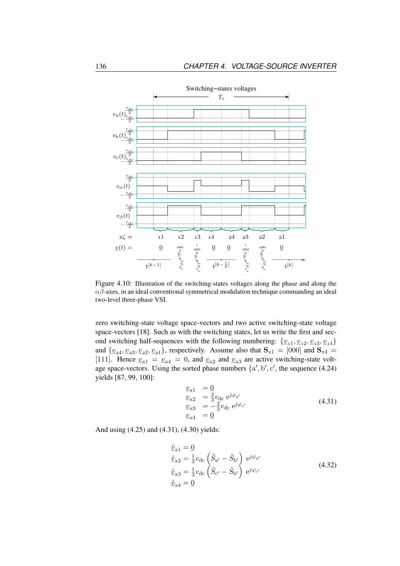
136 CHAPTER 4. VOLTAGE-SOURCE INVERTER
Switching−states voltages
Ts
t[k−1] t[k]t[k−12
]
− vdc2
vdc2
− vdc2
vdc2
− vdc2
vdc2
vdc2
− vdc2
vdc2
− vdc2
12341 2 3 4
00
−23vdcejϕ
c ′
23vdcejϕ
a ′
0 0
23vdcejϕ
a ′
−23vdcejϕ
c ′
vb(t)
va(t)
vc(t)
vα(t)
vβ(t)
xζ =
v(t) =
Figure 4.10: Illustration of the switching-states voltages along the phase and along theαβ-axes, in an ideal conventional symmetrical modulation technique commanding an idealtwo-level three-phase VSI.
zero switching-state voltage space-vectors and two active switching-state voltagespace-vectors [18]. Such as with the switching states, let us write the first and sec-ond switching half-sequences with the following numbering: v1, v2, v3, v4and v4, v3, v2, v1, respectively. Assume also that Sx1 = [000] and Sx4 =[111]. Hence vx1 = vx4 = 0, and vx2 and vx3 are active switching-state volt-age space-vectors. Using the sorted phase numbers a′,b′, c′, the sequence (4.24)yields [87, 99, 100]:
vx1 = 0vx2 = 2
3vdc ejϕa′
vx3 = −23vdc ejϕc′
vx4 = 0
(4.31)
And using (4.25) and (4.31), (4.30) yields:
vx1 = 0
vx2 = 13vdc
(Sa′ − Sb′
)ejϕa′
vx3 = 13vdc
(Sc′ − Sb′
)ejϕc′
vx4 = 0
(4.32)
4.3. ZERO-CROSSING ISSUES AND PREVENTION 137
These results are easily computed from the apriori knowledge of the duty-cycleand the measurement of vdc. The mean active space vectors v2 , v2 + v2 andv3 , v3 + v3 corresponding to an example of v are illustrated in Figure 4.9.
PWM strategies
Using (2.72) with the supply voltages, it yields:
vp = vo + <(v e−jϕp
)(4.33)
where vo is sometimes called the zero-sequence voltage. Introduced this in (4.6)
S?p :=v?o + <
(v? e−jϕp
)vdc
+ 0.5 (4.34)
By the difference in (4.32), this value v?o is simply removed in the active vectorexpression. This value gives therefore a degree of freedom in the selection of thephase duty-cycles [18], and defines the different PWM strategies.
A review of the state-of-the-art about the conventional modulation techniquesat the year of 1999 is given in [99]. It compares the switching loss and har-monic contents of the waveforms. Different strategies for continuous modulationtechnique are compared by [101] regarding the minimization of root mean square(RMS) of the current ripples in induction motors. They are compared regarding thetotal harmonic distortion (TDH) in [102]. Discontinuous modulation techniquesare addressed by [100] regarding the RMS reduction of the current ripples at theDC-bus. Less conventional hybrid modulation techniques are proposed by [108]regarding the current ripples at phase outputs and DC-bus. The maximum voltagein the space-vector frame supplied by the VSI is addressed by [101] for differ-ent strategies. All of these papers give interesting state-of-the-arts concerning themodulation techniques, but they all neglect the nonlinearities of the VSI.
The voltage drops
The voltage drop at the semiconductors of the real VSI can be transposed in themachine model as a constant offset space vector vsc computed using (4.26) fromvsc,p given in (4.10). Details are found in [87, 18, 5, 114].
4.3.2 The Current Ripples
Zero-crossing lines
Assuming no neutral connection, i.e. io = 0, the relation between the space vectorof the currents i and the phase values ip is given by (2.72) in chapter 2 and yields:
ip = <(i e−jϕp
)∀p ∈ a,b, c (4.35)
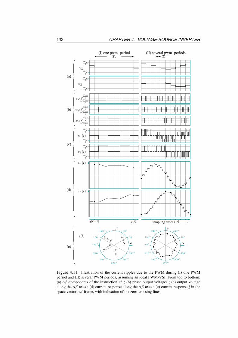
138 CHAPTER 4. VOLTAGE-SOURCE INVERTER
(I) one pwm−period (II) several pwm−periods
(a)
(b)
(c)
(d)
(e)
60
30
330
300
270240
210
180
150
12060
30
330
300
270240
210
180
150
120
Ts
− vdc2
− vdc2
vdc2
− vdc2
vdc2
vdc2
vdc2
− vdc2
vdc2
− vdc2
vdc2
− vdc2
vdc2
− vdc2
i(t)
α
β
α
β
ib=
0
ic =0
ia
=0
Ts
t[k−1] t[k] tsampling times t[k]
vc(t)
va(t)
v?α
v?β
iα(t)
vβ(t)
vα(t)
iβ(t)
vb(t)
Figure 4.11: Illustration of the current ripples due to the PWM during (I) one PWMperiod and (II) several PWM periods, assuming an ideal PWM-VSI. From top to bottom:(a) αβ-components of the instruction v? ; (b) phase output voltages ; (c) output voltagealong the αβ-axes ; (d) current response along the αβ-axes ; (e) current response i in thespace vector αβ-frame, with indication of the zero-crossing lines.
4.3. ZERO-CROSSING ISSUES AND PREVENTION 139
where ϕa = 0, ϕb = 2π/3 and ϕc = 4π/3. It can be deduced that the location of icorresponding to a zero-crossing are along angles ej(ϕp+π/2). They are representedby gray lines in Figure 4.11(e) and Figure 4.12(c). These zero-crossings should beprevented since they lead to inverter nonlinearities that are not compensated.
Due to the pulsewidth modulation (PWM) principle of the voltage source in-verters, described in section 4.2.2, there are small variations of the currents betweentwo samples used by the current controller. These variations are called current rip-ples [102, 99, 108, 101, 100] and are illustrated in Figure 4.11. In the exampleof the illustration, the signals vary with a high frequency close to the PWM fre-quency and a large amplitude regarding the amplitude of the ripples. This couldgive the illusion that computation of the zero-crossing check could be restricted tothe samples. In practice however, the signals controlled by the normal rotation-drive operations (fundamental signals) vary at a much lower frequencies related tothe rotation speed. As a consequency, the current ripples can be much larger thanthe variations between two samples. In signal-injection-based self-sensing meth-ods, the injected signals have high-frequencies close to the PWM frequency, buttheir amplitudes should be as small as possible in order to reduce the impact onthe torque (the goal is also to prevent the emergence of a high-frequency back-emfand to limit the production of noise). As a consequency, the current ripples can bemuch larger than the injected signals. In both case, the current ripples may cross azero-crossing line even if the samples i(t[k]) and i(t[k−1]) do not. This is the mainproblem met with the current ripples that requires to keep a minimum distance be-tween i and the zero-crossing lines. This is illustrated in Figure 4.12 where weassumed much larger ripples regarding the sampling variations.
The first step hereafter is thus to propose an expression of these current ripplesin order to find the minimum margin required between the current samples and thezero-crossing lines such that, ∀p ∈ a,b, c:
sign (ip(t)) = sign(ip(t
[k]))
= sign(ip(t
[k−1]))∀t ∈ [t[k−1], t[k]] (4.36)
The expression of this margin should be as simple as possible to allow quick androbust operations.
Model of the ripples
The current ripples are described in this section using matrix space vectors insteadof complex space vectors. We assume that the current ripples can be modelledby the relation (3.49) addressed in chapter 3, neglecting the eddy currents. Using(4.8), we can link the real and ideal supply voltages by: V ideal = V real + V sc.Removing the subscript “ideal” of V for convenience, we can thus write:
V = LtdI
dt+ E where E =
(R+ ωq
∂L
∂ϕq
)I + EPM + V sc (4.37)
where EPM is the back-emf related to the permanent-magnets. Since we only fo-cus on the current variations dI , that describe the current ripples, we gather all

140 CHAPTER 4. VOLTAGE-SOURCE INVERTER
330
30
60120
150
210
240 300
270
180
0
0
0
vdc2
− vdc2
vdc2
− vdc2
Ts
(a) Supply voltage along αβ
(b) Phase currents
i(t)
(c) Current space-vector and Zero-crossing lines
zero-crossings
zero-crossings
ib(t)
ic(t)
ia(t)
vβ(t)
vα(t)
β
α
ib=
0
ic =0
ia
=0
t[k−1] = t0 t0 = t[k]t1 t1t2 t2tx4t3 t3
t2
t1
t3
t1
t2
t3
t[k−1] = t0
t0 = t[k]t4 = t4
Figure 4.12: Assuming an ideal PWM-VSI, illustration of the (b) phase current responseto (a) PWM voltage and (c) corresponding space vector of the currents i crossing the zero-crossing line ib = 0 in the space vector αβ-frame.

4.3. ZERO-CROSSING ISSUES AND PREVENTION 141
the other components in a temporary value E. This expression (4.37) neglects theeddy current contribution. As it was shown in chapter 3 however, they are not neg-ligible in the experimental BLDC motor. Moreover, the value of the discrete-timeparameters may differs from the continuous-time expression. In first approxima-tion however, we assume that the model (4.37) is valid by approaching Lt withthe apparent discrete-time high-frequency inductance. The resistive voltage dropshould be separated in two contributions: one related to the operating current, us-ing the low-frequency continuous-time resistance ; another related to the currentripples, that could be approached by the apparent discrete-time high-frequency re-sistance. This is further addressed. In order to compute the current ripples, (4.37)is therefore rewritten:
dI = L−1t (V − E) dt (4.38)
At every carrier cycle period of the PWM, for each switching subperiod ξ, the timeintegral of (4.38) yields:
δIξ = L−1t
(∫SξTs
V dt−∫SξTs
Edt
)(4.39)
where δIξ = I(tξ)− I(tξ−1) defines the current back-difference between the endtξ and the beginning tξ−1 of the subperiod. Since the voltage V is constant duringevery subperiod, its integration can be replaced by V ξSξTs that is equal to V ξTs
using the definition (4.32). Keeping a similar notation, we propose to define EξTs
as the integration result of E during the subperiod. Therefore, (4.39) yields:
δIξ = L−1t V ξTs︸ ︷︷ ︸δIV,ξ
−L−1t EξTs︸ ︷︷ ︸δIE,ξ
(4.40)
where we defined δIV,ξ and δIE,ξ as virtual current variations due to the contri-butions of V and E respectively. The points reached by the current ripples duringevery subcycle are found at the instants tξ. The sign of their phase values definethe zero-crossing check: ∀p ∈ a, b, c
sign(ip(tξ)) = sign(ip(t0)) ∀ξ ∈ 1..n (4.41)
However their computations are not straightforward. The value δIV,ξ can be com-puted from the PWM calculator during every subcycle. But δIE,ξ are unknown andmay change at every subcycle. Moreover, since only the initial and final current val-ues of the carrier cycle are sampled, the computation of the current after every sub-cycle would cumulate any error from previous subcycles. A zero-crossing checkwould therefore be inaccurate. We propose therefore another checking methodthat consist to determine a margin around the current samples, that can be largerthan the real ripples. While the margins between the current samples and the zero-crossing lines are satisfied, no zero-crossing should occurs. The main difficulty

142 CHAPTER 4. VOLTAGE-SOURCE INVERTER
consists to fix these margins without two criteria: 1) a quick and reliable computa-tion method regarding all the possible distortions, error and noise sources ; 2) thesmallest possible margin.
Two methods are proposed hereafter. The first one comes from [125]. It isdescribed for information only since it was not retained for several annoying draw-backs: the margins are largely overestimated, they change at every subcycle andrequire to be continuously recomputed. The second one is more approximate, butoffers a smaller margin that is fixed for a constant amplitude of the instructioncurrent and a constant speed.
4.3.3 The Margin Estimation - previous method
This method was published in [125]. Using complex space vectors, the principleconsists to use the virtual currents defined in (4.40), as boundary points to the cur-rent ripples. Using the numbering xζ as introduced in section 4.3.1 and summingall the δixζ during the different subperiods of one PWM carrier half-cycle x andusing (4.40) yields:
δix =
4∑ζ=1
δixζ =
4∑ζ=1
δiv,xζ −4∑ζ=1
δie,xζ (4.42)
Using (4.32) with (4.40), we have δiv,x1 = δiv,x4 = 0. Let us also define thevirtual current variation due to e during the half-cycle:
δie,x ,4∑ζ=1
δie,xζ (4.43)
We therefore can write (4.42) as follows:
i(tx4)− i(tx0) = δix = δiv,x2 + δiv,x3 − δie,x (4.44)
The virtual currents δiv,x2 and δiv,x3 are computed using (4.40) with the VSI activevoltages vx2 and vx3 respectively, that are themselves computed using (4.32). Thevirtual current δie,x can be deduced from (4.44) assuming that i(tx0) and i(tx4) areknown. The currents are sampled at t0 = t[k−1] and t0 = t[k], but generally nosampling occurs at the half-cycle time t4 = t4. By approximation however, weassume that the modulation is symmetric. Thus both half-cycles are symmetricaland we can assume that tx4 = (t0 + t0)/2.
Assume that the virtual currents δie,xζ contribute all to the total δie,x in thesame directions along the different phases. It means that there is no inversionof the virtual currents during the carrier cycle. This condition can be written asfollows:
sign(δip,e,x) = sign(δip,e,xζ)|δip,e,x| ≥ |δip,e,xζ |
(4.45)
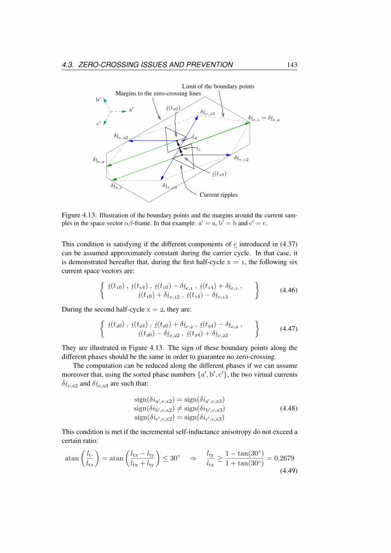
4.3. ZERO-CROSSING ISSUES AND PREVENTION 143
i
i
δie, = δie,
δiv,3
δiv,2
δiv,3
δiv,2
δie,
δie,
i(t0)
i(t0)a′
b′
c′
Current ripples
Limit of the boundary pointsMargins to the zero-crossing lines
Figure 4.13: Illustration of the boundary points and the margins around the current sam-ples in the space vector αβ-frame. In that example: a′ = a, b′ = b and c′ = c.
This condition is satisfying if the different components of e introduced in (4.37)can be assumed approximately constant during the carrier cycle. In that case, itis demonstrated hereafter that, during the first half-cycle x = , the following sixcurrent space vectors are:
i(t0) , i(t4) , i(t0)− δie, , i(t4) + δie, ,
i(t0) + δiv,2 , i(t4)− δiv,3
(4.46)
During the second half-cycle x = , they are:i(t0) , i(t4) , i(t0) + δie, , i(t4)− δie, ,
i(t0)− δiv,2 , i(t4) + δiv,3
(4.47)
They are illustrated in Figure 4.13. The sign of these boundary points along thedifferent phases should be the same in order to guarantee no zero-crossing.
The computation can be reduced along the different phases if we can assumemoreover that, using the sorted phase numbers a′,b′, c′, the two virtual currentsδiv,x2 and δiv,x3 are such that:
sign(δia′,v,x2) = sign(δia′,v,x3)sign(δib′,v,x2) 6= sign(δib′,v,x3)sign(δic′,v,x2) = sign(δic′,v,x3)
(4.48)
This condition is met if the incremental self-inductance anisotropy do not exceed acertain ratio:
atan
(lt-
lt+
)= atan
(ltx − ltyltx + lty
)≤ 30 ⇒ lty
ltx≥ 1− tan(30)
1 + tan(30)= 0.2679
(4.49)

144 CHAPTER 4. VOLTAGE-SOURCE INVERTER
330
30
60120
150
210
240 300
270
180
i(t)
β
α∆im,c
∆im,
b
∆im,a
Figure 4.14: Illustration of the margins transposed around the zero-crossing lines in thespace vector αβ-frame.
The experimental BLDC motor satisfies this conditions with anisotropic ratio around0.66. If the conditions (4.45) and (4.48) are satisfied, it is demonstrated that theboundary points whose sign must be checked are reduced to:
along p = a′ :ia′(t0) , ia′(t0)− δia′,e, , ia′(t4) + δia′,e, , ia′(t4)
along p = b′ :
ib′(t0) + δib′,v,2 , ib′(t0) + δib′,v,3 ,
ib′(t4)− δib′,v,2 , ib′(t4)− δib′,v,3
along p = c′ :
ic′(t0) , ic′(t0)− δic′,e, , ic′(t4) + δic′,e, , ic′(t4)
(4.50)
and for the second half-cycle:
along p = a′ :ia′(t0) , ia′(t0) + δia′,e, , ia′(t4)− δia′,e, , ia′(t4)
along p = b′ :
ib′(t0)− δib′,v,2 , ib′(t0)− δib′,v,3 ,
ib′(t4) + δib′,v,2 , ib′(t4) + δib′,v,3
along p = c′ :
ic′(t0) , ic′(t0) + δic′,e, , ic′(t4)− δic′,e, , ic′(t4)
(4.51)
These points can be checked geometrically by the projection of the boundary points,illustrated in Figure 4.13, along the phase axes.
The zero-crossing margins are computed from these points and correspond tothe distance between the current samples ip(tx0), ip(tx4) and the boundary points.For convenience, they can be transposed along the zero-crossing lines, as illustratedin Figure 4.14. In order to simplify the computation of the margin, we assumethat the ripples are much large than the variation between two consecutive current

4.3. ZERO-CROSSING ISSUES AND PREVENTION 145
samples. It can be written: ip(tx0) = ip(tx4). The margins are therefore:
along p = a′ : ∆im,a′ := |δip,e,a′ |along p = b′ : ∆im,b′ := max
(|δib′,v,x2| , δib′,v,x3
)along p = c′ : ∆im,c′ := |δip,e,c′ |
(4.52)
Benefits of this method: no need to estimate the values contained in e, such as theback-emf and the voltage drops. Drawbacks: the margins are overestimated, theymust be recomputed after every carrier cycle and they are sensitive to VSI timedelays and to the dc-bus voltage measurement. Moreover, the margins computedusing (4.52) do not take into account the oscillations due to the high-frequencysignal than can be injected for the self-sensing in addition to the low-frequencysignal used for the rotation-drive.
Demonstrations
It is demonstrated here that the points (4.46) are bounding the current ripplesreached after every subcycle of the first half-cycle x = . The demonstrationfor the second half-cycle follows exactly the same principle. During the subcycleζ = 1, since δip,v,x1 = 0 and using (4.45), it is shown that ip(t1) along the phasep is limited by the following boundaries:
ip(t1) = ip(t0)− δip,e,1⇒ ip(t1) ∈ [ip(t0) , ip(t0)− δip,e,] (4.53)
During the subcycle ζ = 4, since δip,v,4 = 0 and using (4.45), it is shown thatip(t3) is in:
ip(t3) = ip(t4) + δip,e,4
⇒ ip(t3) ∈ [ip(t4) , ip(t4) + δip,e,] (4.54)
For the middle point ip(t2), the result is:
ip(t2) = ip(t0) + δip,v,2 − δip,e,1 − δip,e,2ip(t2) = ip(t4)− δip,v,3 + δip,e,4 + δip,e,3
⇒ ip(t2) ∈ [ip(t0) + δip,v,2 , ip(t4)− δip,v,3] (4.55)
These points form the boundaries of the ripples given (4.46).Using (4.48), the number of boundary points can be further reduced. For this,
we start with the relation (4.44) along the phase p:
ip(t4)− ip(t0) = δip,v,2 + δip,v,3 − δip,e, (4.56)
Along p = a′ or c′, the boundary point ip(t0) + δip,v,2 is limited by two otherboundary points:
ip(t0) + δip,v,2 = ip(t4) + δip,e, − δip,v,3⇒ ip(t0) + δip,v,2 ∈ [ip(t0) , ip(t4) + δip,e,] (4.57)

146 CHAPTER 4. VOLTAGE-SOURCE INVERTER
and the boundary point ip(t4)− δip,v,3 is in:
ip(t4)− δip,v,3 = ip(t0)− δip,e, + δip,v,2
⇒ ip(t4)− δip,v,3 ∈ [ip(t4) , ip(t0)− δip,e,] (4.58)
It is therefore not required to check these points along a′ and c′. Along p = b′, ityields:
ip(t0) ∈ [ip(t0) + δip,v,2 , ip(t0) + δip,v,3] (4.59)
andip(t4) ∈ [ip(t4)− δip,v,2 , ip(t4)− δip,v,3] (4.60)
Moreover:
ip(t0)− δip,e, ∈ [ip(t4)− δip,v,2 , ip(t4)− δip,v,3] (4.61)
andip(t4) + δip,e, ∈ [ip(t0) + δip,v,2 , ip(t0) + δip,v,3] (4.62)
It is therefore not required to check these points along b′. This leads to the bound-aries mentioned in (4.50).
4.3.4 The Margin Estimation - simplified method
In this simplified method, the issue of the high-frequency and low-frequency com-ponents of the current signal are analyzed separately. We assume that their corre-sponding margins required to prevent the zero-crossing can be summed in order toprovide the total margin.
Low-frequency margin
For the low-frequency components, we assume that the current variations are muchsmaller than the ripples, as in the previous method: i(tx0) = i(tx4). The marginsare however not computed for any position of the current space vector, but onlyaround the zero-crossing lines. The computation is based on the value e only, andnot on the supply voltage anymore. The benefit is that the computation of theswitching voltages at every carrier cycle is not required anymore, but the drawbackis that an estimation of e is needed. The contributions of ri, ePM and vsc in e areanalyzed, but ωq
∂L∂ϕq
is neglected. Note that we make the approximation of an idealsymmetrical modulation. For reason of uniformity in the notations, we maintainthe index of the half-cycle (with the index x = hereafter), but the results areindependent on this index.
The margins that should be kept between the current samples and the zero-crossing lines vary as a function of the current values. In order to give a simple so-lution, we make the assumption that the largest margin would be found for currentsamples located on a zero-crossing line, assuming not inverter nonlinearity. The

4.3. ZERO-CROSSING ISSUES AND PREVENTION 147
30
330
30
60120
150
210
240 300
270
180
30
δie,,d
δie,
∆im,II
∆im
∆im,II
(b)
0
0
(c)
i(t)
∆im
∆im
∆im
0
δie,,q
δiv,2
δiv,3
i(t0)
γ(a)
∆im,I
d ≈y
q ≈x
αib
=0
ia
=0
β
α
ib=
0
ia
=0
ic =0
αib
=0
ic =0
ia
=0
Figure 4.15: Illustration of the margin ∆im := ∆im,I + ∆im,II transposed around thezero-crossing line ib = 0 in the space vector αβ-frame. Geometrical construction of (a)∆im,I alone and (b) with ∆im,II . (c) Illustration of a current space-vector close to 0,where the zero-crossing margin seems to be valid with respect to multiple zero-crossinglines.
148 CHAPTER 4. VOLTAGE-SOURCE INVERTER
margin is therefore computed for current virtually located at these positions, evenif the current should be kept outside this margin in practice. In that location and ne-glecting any anisotropy on the resistance r, the resistive voltage drop ri, computedwith the sample i(t0), is parallel to the zero-crossing line and directed towardzero 0. We neglect here the current ripple contribution to the resistive voltage drop.Assume also that the current is controlled along the quadratic q-axis and that theback-emf ePM = jωdψPM
is along the q-axis oriented toward zero 0, i.e. the shiftbetween the PM magnetic flux ψ
PMand the d-axis is neglected. As a consequence,
ePM and ri both act in the same direction along the q-axis. While no zero-crossingoccurs, the semiconductor voltage drop vsc is a constant space vector oriented byan angle of 30 with respect to the zero-crossing line and towards this line. Its con-tribution along the q-axis is therefore equal to |vsc| cos(30) = |vsc|
√3/2. Adding
this contribution of the vsc, the virtual current variation along the q-axis is:
δie,,q :=1
ltq
(r|i(to)|+ ωd|ψPM
|+√
3
2|vsc|
)Ts
2(4.63)
where Ts/2 is the period of the carrier half-cycle and where ltq is the value of theincremental self-inductance along the q-axis. This virtual current is illustrated inFigure 4.15(a) with the current samples located on the line ib = 0 (the result is thesame along any zero-crossing line) and neglecting the contribution of the vsc alongthe d-axis: δie, = δie,,qejϕq . This contribution along the d-axis is introducedhereafter. Assuming that the samples are fixed, this virtual current variation δie, iscompensated by the virtual current variations δiv,2 and δiv,3 related to the activeswitching voltages. These virtual currents are oriented by an angle γ symmetricallyone either side of the zero-crossing line. If the incremental self-inductance has noanisotropy, this angle is γ = 30. In case of anisotropy, this angle should beslightly smaller. We propose therefore to use the overestimated angle γ = 30 forthe margin computation:
|δiv,2| cos (30) = |δiv,3| cos (30) =δie,,q
2(4.64)
The margin to keep is equal to the component of δiv,2 or δiv,1 perpendicular tothe zero-crossing line:
∆im,I := |δiv,2| sin (30) =δie,,q
2tan (30) =
1√3δie,,q (4.65)
It is illustrated in Figure 4.15(a). Consider the semiconductor voltage drop alongthe d-axis: |vsc| sin(30) = |vsc|/2. Since there is not other contribution, thevirtual current variation along the d-axis is thus:
δie,,d :=1
ltd
(1
2|vsc|
)Ts
2(4.66)

4.3. ZERO-CROSSING ISSUES AND PREVENTION 149
It is illustrated in Figure 4.15(b) with the current samples located at the limit withthe margin. An margin additional margin is approached by this virtual current:
∆im,II := δie,,d (4.67)
The total margin is then the sum of the two proposed margins:
∆im := ∆im,I + ∆im,II
=Ts
2√
3 ltq
(r|i(to)|+ ωd|ψPM
|)
+Ts
4
(1
ltq+
1
ltd
)|vsc| (4.68)
This is illustrated in Figure 4.15(b). This margin is proposed with respect to onezero-crossing line, in the illustration it is ib = 0. For very small operating currenthowever, the possibility of zero-crossing with respect to another zero-crossing lineshould also be analyzed. From simulations, it seemed however that the proposedmargin prevent from multiple zero-crossing. It is illustrated in Figure 4.15(c).
Remember that these computation are performed for a current that is virtuallylocated along a zero-crossing line, but it is independent to the real position of thecurrent. The only values that are required for this computation are those used in(4.68). Note that overestimated parameters r, ωd, l−1
tq and l−1td are valid. Note
that issues regarding the resolution and the measurement noise must be consideredif the resistive voltage drop is computed using current samples. To remove thatproblem, we propose to simply use the current instruction instead of the samples.
High-frequency margin
The additional margin linked to the high-frequency digital signal ∆im,hf is simplyapproached as the biggest magnitude of the high-frequency digital current-responseihf :
∆im,hf = |ihf | (4.69)
This is a strong approximation, but this solution was satisfying during experimentswith our experimental machine. The total margin is then the low-frequency margin∆im,lf given in (4.68) plus ∆im,hf :
∆im := ∆im,lf + ∆im,hf
=Ts
2√
3 ltq
(r|i(to)|+ ωd|ψPM
|)
+Ts
4
(1
ltq+
1
ltd
)|vsc|+ |ihf | (4.70)
Restrictions of the methods
The method is restricted to vector control where the current is controlled along theq-axis. The proposed zero-crossing prevention, introduced hereafter, add an offsetto the current instruction that is partly oriented along the d-axis. So we deviate
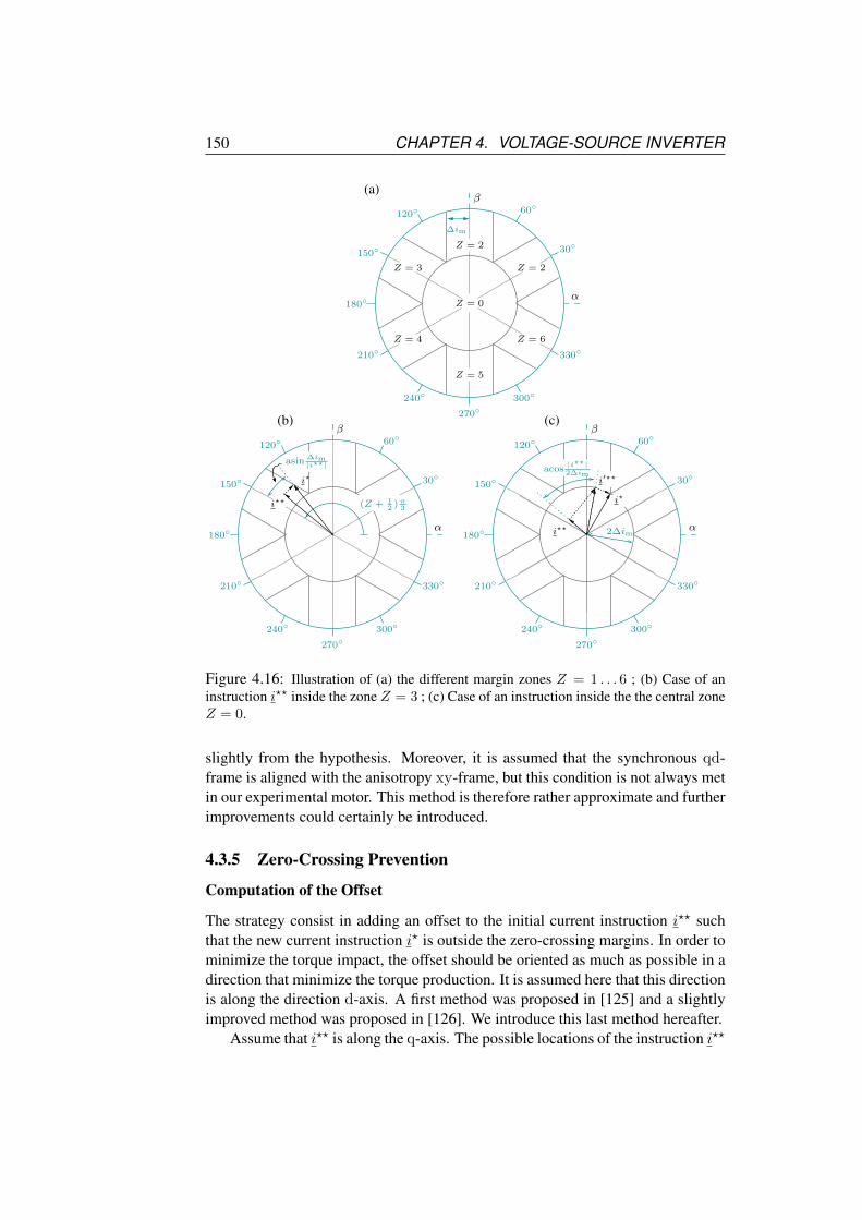
150 CHAPTER 4. VOLTAGE-SOURCE INVERTER
∆im
210
180
120
150
240
270300
330
30
60
210
180
120
150
240
270300
330
30
60
210
180
120
150
240
270300
330
30
60
(a)
(c)
i?? 2∆im
acos|i??|2∆im
i′??
i?
(b)
(Z + 12 )π3
asin ∆im|i??|
i??
i?
Z = 2
Z = 0
Z = 5
Z = 2
Z = 6Z = 4
Z = 3
β
α
β
α
β
α
Figure 4.16: Illustration of (a) the different margin zones Z = 1 . . . 6 ; (b) Case of aninstruction i?? inside the zone Z = 3 ; (c) Case of an instruction inside the the central zoneZ = 0.
slightly from the hypothesis. Moreover, it is assumed that the synchronous qd-frame is aligned with the anisotropy xy-frame, but this condition is not always metin our experimental motor. This method is therefore rather approximate and furtherimprovements could certainly be introduced.
4.3.5 Zero-Crossing Prevention
Computation of the Offset
The strategy consist in adding an offset to the initial current instruction i?? suchthat the new current instruction i? is outside the zero-crossing margins. In order tominimize the torque impact, the offset should be oriented as much as possible in adirection that minimize the torque production. It is assumed here that this directionis along the direction d-axis. A first method was proposed in [125] and a slightlyimproved method was proposed in [126]. We introduce this last method hereafter.
Assume that i?? is along the q-axis. The possible locations of the instruction i??

4.4. EXPERIMENTAL ANALYSIS 151
inside the margins are divided in zones Z, as illustrated in Figure 4.16(a). They arenumbered from 1 to 6 in an anticlockwise order, and the central zone of the marginintersections is numbered Z = 0. The first step consist to compute the zone Zwhere i?? is located. If it is in Z ∈ 1 . . . 6 as illustrated in Figure 4.16(b), wepropose to compute the new instruction i? with the same amplitude but with anangle rotated outside the margin as follows:
|i?| := |i??|∠i? := (Z + 1
2)π3 + sign(∠i?? − (Z + 1
2)π3)
asin∆im|i??|
(4.71)
If the margin size is small compared to the amplitude of the current instruction, theoffset should be along the d-axis in order to keep the impact on the torque small.If Z = 0, as illustrated in Figure 4.16(c), we add a first instruction offset along thed-axis, such that a temporary new instruction i′?? is:
|i′??| := 2∆im
∠i′?? := ∠i?? + acos |i??|
2∆im
(4.72)
and then (4.71) is used with i′?? instead of i?? to compute the second offset. Thissecond offset is not necessarily along the d-axis, resulting in some torque ripplesduring the rotation [125].
Impact of the Offset
There is a discontinuity in the proposed method introduced by the “sign” functionin (4.71). Due to this discontinuity, the new current instruction i? jumps acrossthe margins during the rotation. Assuming a good controller, the jumps should besmall (a few PWM-periods). For the case when the initial instruction is remainingclose to a zero-crossing line, it is strongly advised to compute the “sign” using anhysteresis in order to avoid uncontrollable and repetitive jumps.
In order to reduce as much as possible the current jumps and in order to reducethe torque impact, the margin ∆im should be as small as possible. This is satisfiedas low speed and small controlled currents. When the torque requirements or whenthe speed increase however, the margins can be quite larges. This is the case withour experimental motor.
4.4 Experimental Analysis
4.4.1 Estimation of the Margins
We propose to assess the margin corresponding to the method section 4.3.4 for thecase of the experimental drive. For this, it is required to estimate different valuesand parameters of the test-bench VSI and the experimental machine.

152 CHAPTER 4. VOLTAGE-SOURCE INVERTER
0
2
100 20 30
vsc (V)
isc (A)
Voltage drop at the diode
1
vth = 1.1
rsc ≈ 0.023Ω
0
2
100 20 30
vsc (V)
isc (A)
Voltage drop at the IGBT
1
vth = 1.1
rsc ≈ 0.03Ω
Figure 4.17: Graph of the voltage drop at the semiconductors vsc as a function of thecurrent isc, for the diode and for the IGBT. Linear approximations (plain lines). Standarddeviation of the voltage measurements: 0.17 V.
Dead-time and Voltage drops
The semiconductor voltage drops have been sampled at the beginning of the PWMcycle for 2 × 941 different values of the currents between −30 A and 30 A. Foreach current value, the voltage drop is averaged on about 100 samples. Referringto Figure 4.1, for positive values, the current is flowing through the diode while, fornegative values, it is flowing through the IGBT. Results are shown in Figure 4.17.We see that the voltage threshold is about the same for the diode and the IGBT,uth ≈ 1.1 V, but that the resistance is slightly different. Note that these resistancesrepresent about half the machine resistance mentioned in Table 3.2. For informa-tion, the dead-time is approximately ∆tdt ≈ 4.2µs (4.2% of the PWM-periodTs = 10−4 s−1). For the margin computations, we neglect the dead-time and weapproach the semiconductor voltage drop by the voltage threshold. Using the space
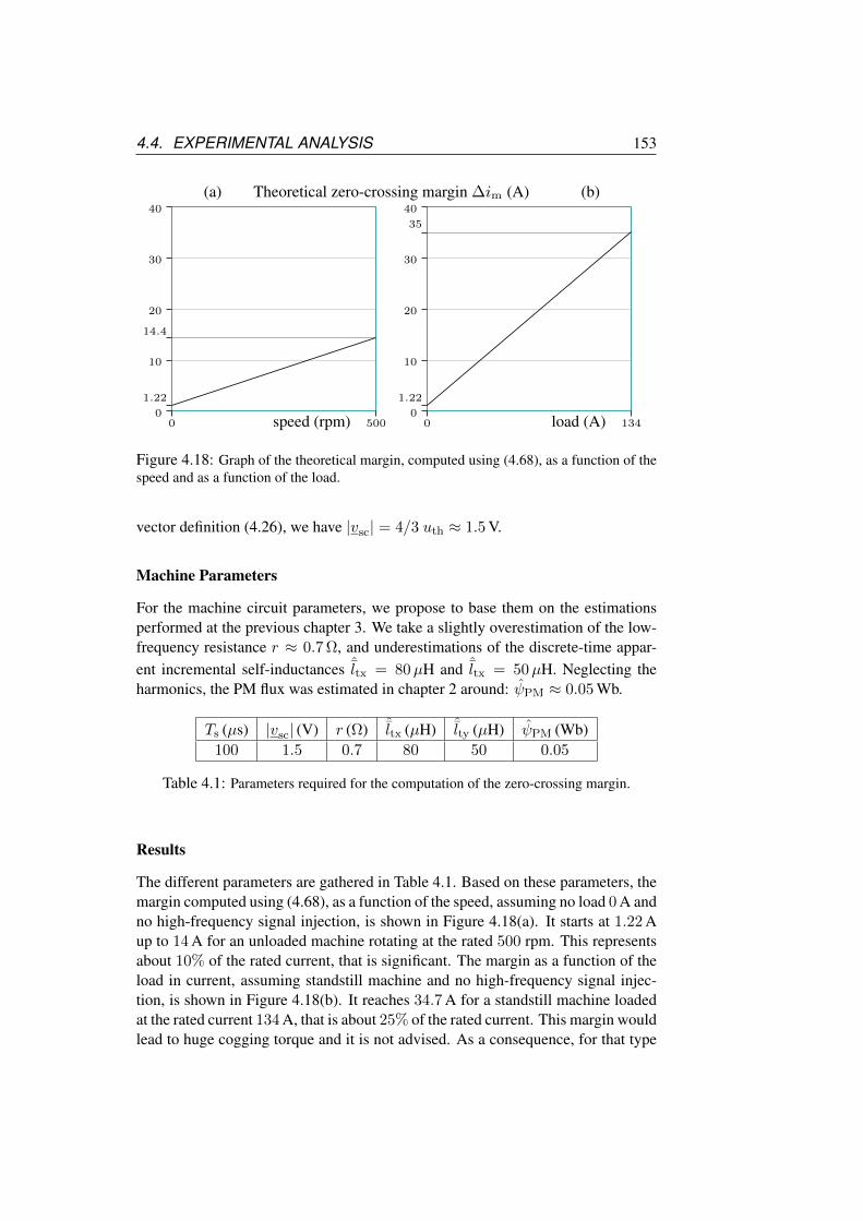
4.4. EXPERIMENTAL ANALYSIS 153
00 500speed (rpm)
10
20
30
40
1.22
14.4
1.22
00 134load (A)
10
20
30
40
35
(a) (b)Theoretical zero-crossing margin ∆im (A)
Figure 4.18: Graph of the theoretical margin, computed using (4.68), as a function of thespeed and as a function of the load.
vector definition (4.26), we have |vsc| = 4/3 uth ≈ 1.5 V.
Machine Parameters
For the machine circuit parameters, we propose to base them on the estimationsperformed at the previous chapter 3. We take a slightly overestimation of the low-frequency resistance r ≈ 0.7 Ω, and underestimations of the discrete-time appar-ent incremental self-inductances ˆltx = 80µH and ˆltx = 50µH. Neglecting theharmonics, the PM flux was estimated in chapter 2 around: ψPM ≈ 0.05 Wb.
Ts (µs) |vsc| (V) r (Ω) ˆltx (µH) ˆlty (µH) ψPM (Wb)100 1.5 0.7 80 50 0.05
Table 4.1: Parameters required for the computation of the zero-crossing margin.
Results
The different parameters are gathered in Table 4.1. Based on these parameters, themargin computed using (4.68), as a function of the speed, assuming no load 0 A andno high-frequency signal injection, is shown in Figure 4.18(a). It starts at 1.22 Aup to 14 A for an unloaded machine rotating at the rated 500 rpm. This representsabout 10% of the rated current, that is significant. The margin as a function of theload in current, assuming standstill machine and no high-frequency signal injec-tion, is shown in Figure 4.18(b). It reaches 34.7 A for a standstill machine loadedat the rated current 134 A, that is about 25% of the rated current. This margin wouldlead to huge cogging torque and it is not advised. As a consequence, for that type
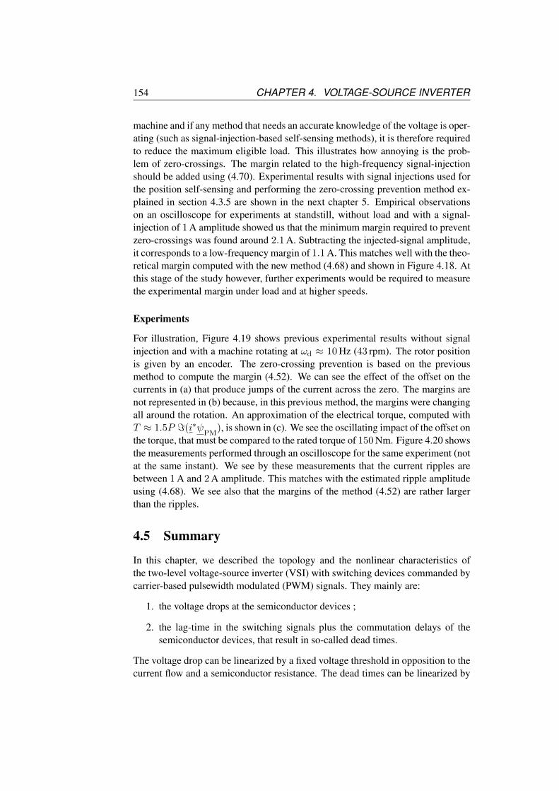
154 CHAPTER 4. VOLTAGE-SOURCE INVERTER
machine and if any method that needs an accurate knowledge of the voltage is oper-ating (such as signal-injection-based self-sensing methods), it is therefore requiredto reduce the maximum eligible load. This illustrates how annoying is the prob-lem of zero-crossings. The margin related to the high-frequency signal-injectionshould be added using (4.70). Experimental results with signal injections used forthe position self-sensing and performing the zero-crossing prevention method ex-plained in section 4.3.5 are shown in the next chapter 5. Empirical observationson an oscilloscope for experiments at standstill, without load and with a signal-injection of 1 A amplitude showed us that the minimum margin required to preventzero-crossings was found around 2.1 A. Subtracting the injected-signal amplitude,it corresponds to a low-frequency margin of 1.1 A. This matches well with the theo-retical margin computed with the new method (4.68) and shown in Figure 4.18. Atthis stage of the study however, further experiments would be required to measurethe experimental margin under load and at higher speeds.
Experiments
For illustration, Figure 4.19 shows previous experimental results without signalinjection and with a machine rotating at ωd ≈ 10 Hz (43 rpm). The rotor positionis given by an encoder. The zero-crossing prevention is based on the previousmethod to compute the margin (4.52). We can see the effect of the offset on thecurrents in (a) that produce jumps of the current across the zero. The margins arenot represented in (b) because, in this previous method, the margins were changingall around the rotation. An approximation of the electrical torque, computed withT ≈ 1.5P =(i∗ψ
PM), is shown in (c). We see the oscillating impact of the offset on
the torque, that must be compared to the rated torque of 150 Nm. Figure 4.20 showsthe measurements performed through an oscilloscope for the same experiment (notat the same instant). We see by these measurements that the current ripples arebetween 1 A and 2 A amplitude. This matches with the estimated ripple amplitudeusing (4.68). We see also that the margins of the method (4.52) are rather largerthan the ripples.
4.5 Summary
In this chapter, we described the topology and the nonlinear characteristics ofthe two-level voltage-source inverter (VSI) with switching devices commanded bycarrier-based pulsewidth modulated (PWM) signals. They mainly are:
1. the voltage drops at the semiconductor devices ;
2. the lag-time in the switching signals plus the commutation delays of thesemiconductor devices, that result in so-called dead times.
The voltage drop can be linearized by a fixed voltage threshold in opposition to thecurrent flow and a semiconductor resistance. The dead times can be linearized by
4.5. SUMMARY 155
0
60
30
330
90120
0
5
10
−5
−10
10 5 0 −5 −10
0
−5
10
5
−10
0
−5
10
5
−10
0
−5
10
5
−10
i(t)
0
−1
5
1
2
3
4
(a) Phase currents (A)
(b) Current space-vector (A)
(c) Electrical torque (Nm)
ia
ib
ic
0 0.01 t (s)0.10.02 0.03 0.04 0.05 0.06 0.07 0.08 0.09
T
Figure 4.19: Experimental results of the zero-crossing prevention method based on themargin (4.52), for a initial current instruction around 1 A along the q-axis. No high-frequency signal is injected. The rotor orientation is given by an encoder. (a) New currentinstruction with the offset (plain lines) and measurements samples of the phase currents(dots) ; (b) Representation of the currents in the space-vector frame ; (c) Electrical torqueapproached using the fundamental space-vector of the PM flux.

156 CHAPTER 4. VOLTAGE-SOURCE INVERTER
0
60
30
330
90120
0
5
10
−5
−10
10 5 0 −5 −10
0
−5
10
5
−10
0
−5
10
5
−10
0
−5
10
5
−10
i(t)
(a) Phase currents (A)
(b) Current space-vector (A)
(c) Electrical torque (Nm)
ia
ib
ic
0 0.01 t (s)0.10.02 0.03 0.04 0.05 0.06 0.07 0.08 0.09
Figure 4.20: Oscilloscope measurements related to the experiment shown in Figure 4.19.

4.5. SUMMARY 157
fixed values with a sign depending on the current flow. The compensation methodsare therefore closely related to the current flow in the different phases. Note how-ever that these nonlinearities, when no phase current crosses zero, are not involvedin the self-sensing operations.
When a phase current crosses zero however, a phenomenon called zero-clampingtends to maintain the current at zero during the dead time. This phenomenon has adramatic impact on the self-sensing operations based on signal injection, and leadsto faulty estimations. No simple and efficient compensation method was found tocompensate this zero-crossing nonlinearity. The solution is even more complicatedthan the current ripples may cross zero even if the current samples do not. It istherefore proposed to maintain the current instruction far enough from the zero-crossing lines and to jump through these lines when required. This solution limitsthe number of zero-crossings and the impact of the nonlinearity.
The first step consist to estimate the required margins. Two methods wereproposed:
1. the first method computes confident margins after every sampling period.The margins are however overestimated and vary during the control opera-tions ;
2. the second method proposes approximate margins, as a function of the statorcurrent amplitude and the speed. This method requires an initial estimationof the stator resistance and an estimation of the PM magnetic flux. Themargin is however smaller and fixed for stead-state operations.
The second step is the implementation of the zero-crossing prevention method.This method adds an offset to the initial current instruction in order to keep thecurrent outside the margins. The offset is selected in order to have a reduced impacton the control operations, but it inevitably produces a small torque. It was shownthat the required margin for the experiment BLDC motor at rated conditions arerather large. This zero-crossing prevention solution requires therefore a reductionof the maximum torque in order to limit the margin amplitude.

158 CHAPTER 4. VOLTAGE-SOURCE INVERTER
Chapter 5
Signal Processing
This chapter addresses the control of the machines and the position-self-sensingsolutions. It details the numerous self-sensing strategies and gives the concreteoperations for the studied case of high-frequency signal-injections used by theanisotropy-based self-sensing method. It is the outcome of the developments initi-ated from the first chapter of this thesis.
5.1 Introduction
The optimal control of PM machines requires the knowledge of the rotor position,that can be measured by external dedicated sensors. However, more and more,these sensors are removed for all the reasons mentioned in the introduction chap-ter 1, leading to so-called self-sensing methods. The principle is to use electrome-chanical phenomenons in the machine itself, that vary with the rotor position, toestimate the rotor position. These phenomenons can be observed and tracked frommeasurable electrical variables, such as currents and voltages.
At high speeds, the back-emf is a reliable source to estimate the rotor positionwithout much effort. Its signal-to-noise quality however decreases with the rotationspeed. At low rotation speed and standstill, an estimation of the rotor position canbe obtained from anisotropic properties linked to the rotor position. As addressedin chapter 2, these anisotropies can be due to variations in the rotor geometry or tomagnetic saturation effects in the iron and are revealed through parameters, suchas the incremental self-inductance. Anisotropy misalignment may appear due tosignificant stator currents and to harmonics in the machines related to harmonicsin the conductor distributions and to nonsinusoidal magnetic-fields.
In the vast majority of anisotropy-based strategies without extra sensors, theanisotropy is tracked performing high-frequency signal injection in addition to therotation-drive operating signals. Many different types of signal injection can beused: test-pulse trains, PWM modifications, carrier-based pulsating and rotating-signals injection. Mathematical developments and comparisons between differentsignal injections are proposed in this chapter.
159

160 CHAPTER 5. SIGNAL PROCESSING
Except in some publications, the resistance impact is often neglected in signal-injection operations, assuming an ideal inductive machine. The eddy currents how-ever increase with the frequency and may significantly affect the apparent resis-tance value, as describe in chapter 3, leading to position-estimation errors. Thisissue is closely related to the frequency of the injected signals. This frequency isoften selected between 400 Hz and 2 kHz [127, 128] and many papers introduceself-sensing using continuous-time operations. We propose here to study discrete-time operations up to one third of the sampling frequency used by the current con-troller, which is the maximum possible frequency defining rotating signals. Thebenefits of the proposed method are analyzed regarding disturbing interactions be-tween the rotation-drive and the self-sensing operations, regarding the filtering andthe computational requirement, the robustness and the impact of the apparent re-sistance.
∼
This chapter is organized as follows: the section 5.2 introduces elementary de-scriptions of the field-orient control. It is attempted to give a large overview of themany different self-sensing, to categorize them and to compared their advantagesand drawbacks ; Section 5.3 addresses the model specially for the high-frequencysignal-injection methods using digital measurements of the terminal currents. Theprinciple, the assumptions and the filtering operations of the signal-injection areintroduced. The position estimations operations are developed for rotating and pul-sating signal injections. A last case of alternating signal injection is also addressed ;Section 5.4 shows experiment results of the self-sensing operations applied on theexperimental BLDC motor ; A summary of the important elements of this chapteris given in section 5.5.
5.2 Self-Sensing Field-Oriented Vector-Control
5.2.1 The Vector-Control Principle
The term vector controls gather all variable-speed control-schemes intended forpolyphase machines and using tools based on the space-vector concept. The currentand voltage values are therefore handled using their transpositions in space vectorframes, either by their complex or their matrix forms. Note that the classification ofa control method in the category of “vector controls” is sometime only a question ofpoint of view: a same processing can be equivalently deduced from phase relationsor space-vector relations. In the case of a three-phase machine without neutralconnection however, the space-vector relations offer generally more intuitive andshorter expressions than the phase relations.
Among the vector controls, we mainly have two strategies:
• the Field-Oriented Control (FOC), described hereafter and assumed in thiswork ;

5.2. SELF-SENSING FIELD-ORIENTED VECTOR-CONTROL 161
• the Direct Torque Controls (DTC) and the more recent Predictive TorqueControls (PTC).
Comparisons between FOC and PTC for induction machines (IM) are proposed by[130, 131]. Comparisons between different PTC, called Optimal Switching TimePTC, hysteresis based PTC and more basic PTC are addressed in [132]. Theyare however not addressed in the frame of self-sensing controls. Review of theadjustable-speed drives, including open-loop scalar controls, are found in [5, 2,1, 7]. Note that the choice of FOC in this work is not due to any performanceconsideration, but simply to the experimental equipment that does not allow toperform PTC.
5.2.2 The Field-Oriented Control
The Field-Oriented Control (FOC) is a vector control generally intended to three-phase synchronous machines, i.e. machines where the harmonics are small com-pared to the fundamental of the flux. In that case, the fundamental space vectorof the flux ψ yields a good approximation of the fundamental coefficient ψ(1), asshown in chapter 2 by (2.50). Combining this approximation with the expressionof the torque applied on the stator (2.69) yields:
T =3P
2=(i∗ψ)
(5.1)
where n is the number of phases and P is the number of pole-pair in the machine.Note that the torque applied on the rotor is −T . This expression (5.1) is validwith space vectors in any reference-frame. This is demonstrated here with thetransposition in the synchronous qd-reference-frame using (3.8), as described inchapter 3: (
i∗ ψ) ∣∣
qd=(i∗ejϕq ψ
e−jϕq
) ∣∣αβ
=(i∗ ψ
) ∣∣αβ
(5.2)
In the case of a permanent-magnet (PM) machine, the flux ψ is made of two con-tributions: one from the stator currents and one from the rotor PM:
ψ = ψS
+ ψPM
(5.3)
On the other hand, the assumption of synchronous machines yields that the PM fluxψ
PMis oriented along the d-axis of the permanent magnet locations (by convention
in a negative direction along this axis). In the synchronous qd-reference-frame, thisyields:
ψPM
∣∣qd
= −jψPM (5.4)
On the other hand, for convenience, it is generally assumed that the synchronousqd-frame is aligned with the anisotropy frame related to the relation linking i toψ
S. In the synchronous qd-reference-frame, this yields:
ψS
= lqiq + jldid (5.5)
162 CHAPTER 5. SIGNAL PROCESSING
Combining these results with i∗|qd = iq − jid, (5.1) yields:
T =3P
2=(
(iq − jid) (lqiq + j(ldid − ψPM)))
⇒ T = −3P
2
((lq − ld)id + ψPM
)︸ ︷︷ ︸
Magnetization
iq (5.6)
A similar expression is found in [1, 114]. A matrix form is found in [133]. As-suming that the magnetization part, made of ψPM and (lq − ld)id, is constant, thisexpression shows that the torque TPM is only function of iq. The q-axis can there-fore also be referred to as the torque axis. Note that some publications in the fieldof PM-machine sensorless control neglect the contribution of the anisotropy to thetorque, such as [79] for the PM-machines and [131] in the case of an inductancemachine. The FOC schemes are illustrated in [79, 1] with flowcharts.
The current id along the d-axis is sometimes used to reduce the magnetic fluxamplitude |ψ| [1]. The goal is to reach higher controllable speeds ωd, assumingthat the command voltage is maintained under the maximum voltage vmax suppliedby the PWM-VSI. This is illustrated as follows. Neglecting resistive voltage drops,inverter nonlinearities and the eddy currents, the voltage v at the machine terminalsin the synchronous qd-reference-frame is:
v|qd ≈ jωdψ|qd ⇒ |v| ≈ |ωd|√
(ldid − ψPM)2 + (lqiq)2 (5.7)
While the speed increases, ωd , the principle consists to increase the currentid such that |v| < vmax. The variations of id are therefore related to the speedωd and are slow regarding the variations of iq performed by the torque controloperations.
As we showed, all these operations are performed with space vectors in the syn-chronous qd-reference-frame, defined with respect to the PM-rotor position. ThePM position can be measured by dedicated sensors, or using estimation methodssuch as the self-sensing methods described hereafter.
The expression of the PM contribution to the torque is complicated if ψPM
isnot oriented along the d-axis and (5.4) is not valid anymore. This is the case inour experimental BLDC motor, but experiments shown in chapter 2 that the fifthharmonic, that was the highest, represented only 1% of the fundamental amplitude.As a consequence, we could neglect the harmonics even in the case of our nonsyn-chronous BLDC motor. Another difference comes from the misalignment betweenthe anisotropy and the synchronous frame. In that case, (5.5) is not valid anymore.As addressed in chapter 2, the misalignment can be due to space harmonics, butalso to the increasing impact of i on the magnetic state. This issue is not easy tohandle since the value of the self-inductance is then required for any rotor positionand any value of i. Moreover, we can not rely on signal-injection methods sincethis method only identify the incremental part of the self-inductance, but not theself-inductance l regarding the total current i.

5.2. SELF-SENSING FIELD-ORIENTED VECTOR-CONTROL 163
Methods taking all these issues into account could certainly be developed, butthis is not the topic of this study. We propose therefore to simply neglect thestator current contribution to the flux in the torque computation, and to assume theapproximation of a synchronous flux for the control operations:
|id| |iq| ⇒ T ≈ −3P
2ψPM iq (5.8)
Note that there are also other sources of torque that are not controlled, suchas the cogging torque or the torque due to the homopolar current. Controlling thehomopolar current can increase the average torque produced during the rotation ifwe have access to the neutral connection [51]. They are however not studied in thisdocument.
5.2.3 Conventional BLDC Control
The conventional control of BLDC-machines differs from FOC [2]. It is often de-scribed from the point of view of the phase values and assuming that the PM-fieldscan be approached by a trapezoidal function along the air-gap. It also neglects theanisotropy and its contribution to the torque. In that case, the torque should remainconstant if opposite currents are injected in the two phases whose conductors are infront of the PM, while no current is injected in the third phase. The phase currentsare therefore commutating during the rotation. Transposed in space vectors, we candefine the torque axis along discrete positions of the PM. The current space vectoris therefore not smoothly rotating with the PM, but jumps between these discretepositions. The commutations are usually initiated by hall-effect sensors that detectinversions of the magnetic field in the air-gap [29].
Our experimental machine is a BLDC motor. It would therefore make sense touse a conventional BLDC control method. Some experiments however showed usthat the FOC produced a much smoother torque than the BLDC control. This issuewas also introduced by [50].
5.2.4 Regulators in Closed-Loop Controls
Details about regulators and observers can be found in many publications [46, 134,10, 11, 135, 36]. This work however does not focus on the regulation issues.All the regulations implemented in the experiments are based on simple discreteproportional-integral operations with anti-wind-up and limited output instructions.The operations are similar to those presented in [136]. Other type of operationsexist, such as sliding-model regulators, but they are not studied in this work. Forthe position estimation filtering, simple Luenberger observers are used, as clearlydescribed by Luenberger himself [137] and by [138], or in more recent publications[134].

164 CHAPTER 5. SIGNAL PROCESSING
Table 5.1: Comparison between the back-emf and the anisotropy as source of rotor-position information.
1. back-EMF 2. AnisotropySpeed range Nonzero speed Any from standstill
Load sensitivity Low StrongHarmonic sensitivity Medium Strong
5.2.5 Sources of Position Information
As discussed previously, the vector controls require the knowledge of the rotor po-sition. Two electromechanical phenomenons in the PM machine model can containrotor-position information:
• the back-electromotive force (back-EMF) ;
• a magnetic anisotropy.
They are compared in Table 5.2.5 and addressed in details hereafter. A huge num-ber of different self-sensing strategies are found in the literature, with names thatare very variable from one publication to the other. Often, the back-EMF-basedmethods are referred to as fundamental model methods [5, 139, 2]. But to ourknowledge, the strategies found are all based on one or both of these sources ofposition information, sometimes with specific issues depending on the machinetypes.
5.2.6 Back-EMF-Based Self-Sensing
The back-EMF is the voltage induced by the time variation of the magnetic fluxproduced from the rotor-side and linked by the stator circuits. It is related to therotor position in any machine having an independent magnetic source at the rotor,generally referred to as synchronous machine. The case of induction machines,also called asynchronous machines, is more complicated since the back-EMF isnot induced from an independent rotor source, but related to a mutual flux and itis function of the shift between the rotor speed and the stator signal frequency.More details about back-EMF-based self-sensing methods in induction machinesare given in [140] with analysis of parameter sensitivity and in [5, 2].
In case of PM, the back-EMF is written: ePM = dψPM/dt. In synchronous
machines where the flux can be approached by its fundamental component, the PMflux is of constant amplitude and aligned with the d-axis: ψ
PM= ψPMejϕd . The
back-EMF is then a reliable source to estimate the rotor position and speed withoutmuch effort [141]:
ePM =dψ
PM
dt= jωdψPMejϕd ⇒
ωd = |ePM|/ψPM
ϕd = ∠(−jePM)(5.9)

5.2. SELF-SENSING FIELD-ORIENTED VECTOR-CONTROL 165
If ψPM is known, the rotation speed ωd is directly deduced. Otherwise, ωd canbe computed using an observer of the dynamic model (not developed here), andthen ψPM could be deduced. Except in [142, 143], note that (5.9) is generally notexplicitly mentioned in most of the publications, but it is integrated in an observerexpression, such as described hereafter.
The back-EMF estimation can be based on one of the machine models devel-oped in chapter 3. Let us analyze this issue from the continuous-time machinemodel without eddy currents in the stationary αβ-frame (3.48):
ePM = v − lt+di
dt− lt-
di∗
dt−(r+ + ωq
∂l+∂ϕq
)i−(r- + ωq
∂l-∂ϕq
)i∗ (5.10)
If the PWM-VSI nonlinearities are compensated, v is known by its command valuev?. The currents i are measured. The computation of ePM then requires accu-rate knowledge of all the parameters appearing in that expression. The expression(5.10) is generally not directly used to compute the back-EMF estimation. In or-der to reduce the noise impact and in order to eventually correct the parametervalues, the use of an observer is advised. Most of the observers found in the litera-ture assume no anisotropy and no variation of the self-inductances as a functionof the position [5]. This is the case with [144] with a stator-flux-based meth-ods using MRAS observer. Other publications take the anisotropy into account[79, 133, 142], or [145] using extended Kalman filters, but assuming constant pa-rameters and assuming that the anisotropy is aligned with the synchronous frame.In [133], the method is improved including the dynamic model of the machine inthe observation. In [133], the method is augmented by a signal-injection that iden-tifies the resistance, that may vary with the temperature. It however neglects anyanisotropic aspects. Taking the anisotropy into account in back-EMF-based meth-ods is however not easy. Anisotropy misalignments can appear if the current load issignificant or if the machine presents important harmonics. Moreover, the harmon-ics result in anisotropic relations oscillating at several times the rotation frequency.This strongly complicates the implementation of an observer. This is the case ofthe experimental BLDC motor. A review of the different types of methods is givenby [5, 2].
As shown by (5.9), the back-EMF magnitude is directly related to the rotorspeed. Therefore, the position estimation accuracy decreases with the speed re-duction, and completely vanishes at standstill. This is the main drawback of thesolutions compared to the anisotropy-based solutions, described hereafter. Someauthors therefore propose methods switching between the two self-sensing solu-tions around a threshold speed [133, 143, 114].
5.2.7 Anisotropy-Based Self-Sensing
Terminal-based circuit model
We focused here on a model linking space vectors of the voltage and current ter-minals, that are sampled by the sensors used by the rotation-drive controller. Self-
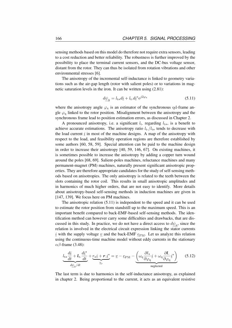
166 CHAPTER 5. SIGNAL PROCESSING
sensing methods based on this model do therefore not require extra sensors, leadingto a cost reduction and better reliability. The robustness is further improved by thepossibility to place the terminal current sensors, and the DC-bus voltage sensor,distant from the rotor. They can thus be isolated from rotation vibrations and otherenvironmental stresses [6].
The anisotropy of the incremental self-inductance is linked to geometry varia-tions such as the air-gap length (rotor with salient poles) or to variations in mag-netic saturation levels in the iron. It can be written using (2.81):
dψS
= lt+di+ lt-di∗ej2ϕx (5.11)
where the anisotropy angle ϕx is an estimator of the synchronous qd-frame an-gle ϕq linked to the rotor position. Misalignment between the anisotropy and thesynchronous frame lead to position estimation errors, as discussed in Chapter 2.
A pronounced anisotropy, i.e. a significant lt- regarding lt+, is a benefit toachieve accurate estimations. The anisotropy ratio lt-/lt+ tends to decrease withthe load current i in most of the machine designs. A map of the anisotropy withrespect to the load, and feasibility operation regions are therefore established bysome authors [60, 58, 59]. Special attention can be paid to the machine designin order to increase their anisotropy [40, 59, 146, 67]. On existing machines, itis sometimes possible to increase the anisotropy by adding a copper turn woundaround the poles [68, 69]. Salient-poles machines, reluctance machines and manypermanent-magnet (PM) machines, naturally present significant anisotropic prop-erties. They are therefore appropriate candidates for the study of self-sensing meth-ods based on anisotropies. The only anisotropy is related to the teeth between theslots containing the rotor coil. This results in small anisotropic amplitudes andin harmonics of much higher orders, that are not easy to identify. More detailsabout anisotropy-based self-sensing methods in induction machines are given in[147, 139]. We focus here on PM machines.
The anisotropic relation (5.11) is independent to the speed and it can be usedto estimate the rotor position from standstill up to the maximum speed. This is animportant benefit compared to back-EMF-based self-sensing methods. The iden-tification method can however carry some difficulties and drawbacks, that are dis-cussed in this study. In practice, we do not have a direct access to dψ
S, since the
relation is involved in the electrical circuit expression linking the stator currentsi with the supply voltage v and the back-EMF ePM. Let us analyze this relationusing the continuous-time machine model without eddy currents in the stationaryαβ-frame (3.48):
lt+di
dt+ lt-
di∗
dt︸ ︷︷ ︸dψ
S/dt
+ r+i+ r-i∗︸ ︷︷ ︸
vr
= v − ePM −(ωq
∂l+∂ϕq
i+ ωq∂l-∂ϕq
i∗)
︸ ︷︷ ︸neglected
(5.12)
The last term is due to harmonics in the self-inductance anisotropy, as explainedin chapter 2. Being proportional to the current, it acts as an equivalent resistive

5.2. SELF-SENSING FIELD-ORIENTED VECTOR-CONTROL 167
contribution, with the oscillating value, that could be mixed with the stator resistor.No publication found by the author manage this term, that is generally neglected[143]. We propose also to neglect it at this stage of the study, but its impact isquickly assessed at the end of this subsection.
As we can see in (5.12), the incremental self-inductance is not the only possibleanisotropy source of this relation. Chapter 3 introduced the fact that the statorresistance can also present an anisotropy due to unbalancing between the differentphase resistances, but this anisotropy is not linked to the rotor position. It washowever showed that eddy currents, or any additional circuit placed in the rotor[68, 69], influence the apparent parameter values of the circuit model. In particular,the apparent resistance for high-frequency signals could largely increase in relationwith a magnetic anisotropy linked to the rotor position. This effect is used insome publications to develop self-sensing methods based on resistance-anisotropy[148, 85, 149]. As discussed in chapter 3, this strategy should however be assessedwith respect to discretization and PWM distortions. Assuming that the anisotropyangles of the incremental self-inductance and the resistance are equal, (5.12) canbe written: (
lt+di
dt+ r+i
)+
(lt-di
dt+ r-i
)∗ej2ϕx = v − ePM (5.13)
The low frequency signals used by the rotation-drive operations are generally notadequate to perform self-sensing estimations. In one hand, the current variationsdi/dt are small compared to the measurements noise, leading to inaccurate esti-mations. On the other hand, the back-EMF is apriori unknown. In the vast ma-jority of anisotropy-based methods, the solution to overcome these issues consiststo use self-sensing estimations based on signals having higher frequencies thanthe rotation-drive operating signals (also sometimes referred to as “fundamental”operating signals) [5]. The self-sensing operations are then based on the relationbetween high-frequency signals, denoted here by hf . Higher the frequency, higherthe contribution of dihf/dt with respect to i and to the noise. As a consequence,a large number of methods found in publications neglect the resistive contribution.Moreover, the contribution of the high-frequency signals to the back-EMF tends todecrease, such that ePM,hf is neglected in the high-frequency model. These pointsare further discussed in section 5.3. Therefore, (5.13) simply yields:
lt+dihf
dt+ lt-
di∗hf
dtej2ϕx ≈ vhf (5.14)
Since the injected high-frequency voltage vhf is known and since ihf can be mea-sured, it is possible to identify the anisotropy angle ϕx. The method to extract ϕx
depends on the type of signal. This is addressed in the next section 5.2. The impactof significant resistance on the self-sensing operations assuming this approxima-tion is also addressed in this chapter.

168 CHAPTER 5. SIGNAL PROCESSING
Table 5.2: Comparison between solutions with extra sensors dedicated to the self-sensingoperations and solutions using the terminal values.
1. Terminal-based 2. Dedicated sensorsType Control sensors Specifically selected
Accuracy Lower IncreasedReliability Strong Lower
Assessment of the impact from self-inductance variations
The impact of the neglected part in (5.12) is quickly assessed in the case of theexperimental machine. For this, we assume that the harmonic content of the self-inductance should be lower in amplitude than the harmonic content of its incre-mental part. Therefore, the assessment is based on the incremental self-inductance,considered as an upper limit. Using the results of the experimental BLDC machinepresented chapter 2, it was shown that lt,+ is quite constant: ∂l+/∂ϕq ≈ 0 ; andthat lt,- only contains significant harmonics at k = 2 and k = −4. Neglecting themisalignment due to the current load, it yields:
lt- = lt,(2)ej2ϕq + lt,(−4)e
−j4ϕq (5.15)
⇒ ωq∂lt-
∂ϕq= 2ωqlt,(2)e
−j4ϕq − 4ωqlt,(−4)e−j4ϕq (5.16)
where |lt,(2)| ≈ 23µH and |lt,(−4)| ≈ 3µH. At the rated speed of the motor,ωq = 2π × 116 = 729 rad/s. Therefore:
|2ωqlt,(2)| ≈ 0.034 Ω
|4ωqlt,(−4)| ≈ 0.009 Ω(5.17)
These results are lower than resistance, that varies between 0.05 Ω for DC sig-nals and 0.15 Ω for 3.33 kHz signals. We assume therefore that if the resistancecontribution is small, then the self-inductive-variations contribution should also besmall.
Dedicated-sensor solutions
Other solutions based on extra sensors are however possible. The drawback of ex-tra sensors are always the sames: additional source of possible failure, additionalsetup and cost. However, if dedicated to the self-sensing operations, the resolutionof these extra sensors can be adapted to the small amplitude of the high-frequencysignals used to identify the anisotropy angle [105]. This can be especially advisedfor machines presenting very small anisotropic properties, such as induction motors(IM). For example, [147, 139] use the zero-sequence current response flowing in adelta-connected stator circuit of IM. The main risk concerns the reliability because

5.2. SELF-SENSING FIELD-ORIENTED VECTOR-CONTROL 169
Table 5.3: Comparison between different sources of high-frequency signals.
1. DTC/PTC 2. PWM 3. Signal-InjectionCommand Subordinated Subordinated Free (∗)
High-frequency / ωc ≪ ωs < ωhf ωc ωhf < ωs
Measurements Samples Additional SamplesModel sensitivity High Low Low
Symbols: Usable high-frequencies ωhf ; rotation-drive frequency ωc ; sampling frequencyωs. Note: (∗) in the limit of the eligible voltages by the VSI and on the maximum current.
this sensor is placed in the stator circuit of the machine, and undergoes environ-mental stresses. It is also possible to use the zero-sequence voltage for self-sensingoperations, as proposed in [150, 66, 105].
Note that some publications mention the use of current-slope sensors. Thesesensors can be dedicated [139, 151] or simply included in some newer sensorsalso used for the rotation-drive control operations. The issue of the noise in suchcurrent-slope measurements must however seriously be studied.
We also mentioned some alternative solutions: [77] proposes a solution basedon an independent high-frequency supplier. This solution therefore requires alsoadditional setup of the separated supply. [152] proposes to use a back-EMF detec-tion circuit for the commutation of the currents in a BLDC motor control. [153]proposes a low cost solution by the measurement of the DC-bus current.
5.2.8 High-Frequency Sources
Let us analyze three sources of high-frequency signals that could be used for self-sensing operations. They are summarized in Table 5.2.8:
1. The high-frequency signals can be naturally produced by the rotation-driveoperations, even if they are not used for the rotation drive. This is the caseof the ripples in DTC and in PTC. The self-sensing operations can be per-formed using the current samples used for the control, without additionalsamplings. The high-frequency signal is however subordinated to the hys-teresis method of the torque controller and it is therefore not independentlycommanded in time and amplitude. Moreover, that type of self-sensingstrategy is significantly sensitive to the model parameters, such as the re-sistance and the back-EMF that must be known since they contribute to thecurrent variations. Self-sensing methods using DTC signals or PTC signalsare developed in [154, 155, 156]. Another type of controls such as the Cur-rent Hysteresis Chopping Control intended for switched reluctance motor(SRM) supplied by asymmetrical half bridge power converter may also pro-vide high-frequency signals reliable for self-sensing operations, as proposedby [157].
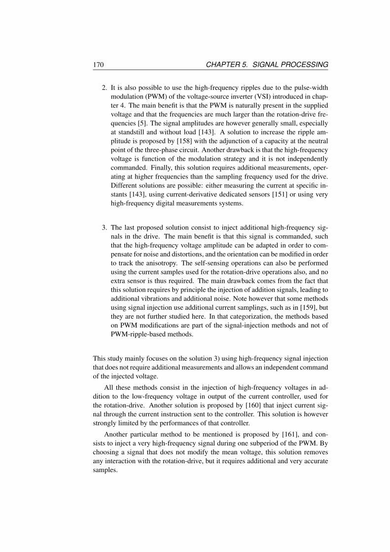
170 CHAPTER 5. SIGNAL PROCESSING
2. It is also possible to use the high-frequency ripples due to the pulse-widthmodulation (PWM) of the voltage-source inverter (VSI) introduced in chap-ter 4. The main benefit is that the PWM is naturally present in the suppliedvoltage and that the frequencies are much larger than the rotation-drive fre-quencies [5]. The signal amplitudes are however generally small, especiallyat standstill and without load [143]. A solution to increase the ripple am-plitude is proposed by [158] with the adjunction of a capacity at the neutralpoint of the three-phase circuit. Another drawback is that the high-frequencyvoltage is function of the modulation strategy and it is not independentlycommanded. Finally, this solution requires additional measurements, oper-ating at higher frequencies than the sampling frequency used for the drive.Different solutions are possible: either measuring the current at specific in-stants [143], using current-derivative dedicated sensors [151] or using veryhigh-frequency digital measurements systems.
3. The last proposed solution consist to inject additional high-frequency sig-nals in the drive. The main benefit is that this signal is commanded, suchthat the high-frequency voltage amplitude can be adapted in order to com-pensate for noise and distortions, and the orientation can be modified in orderto track the anisotropy. The self-sensing operations can also be performedusing the current samples used for the rotation-drive operations also, and noextra sensor is thus required. The main drawback comes from the fact thatthis solution requires by principle the injection of addition signals, leading toadditional vibrations and additional noise. Note however that some methodsusing signal injection use additional current samplings, such as in [159], butthey are not further studied here. In that categorization, the methods basedon PWM modifications are part of the signal-injection methods and not ofPWM-ripple-based methods.
This study mainly focuses on the solution 3) using high-frequency signal injectionthat does not require additional measurements and allows an independent commandof the injected voltage.
All these methods consist in the injection of high-frequency voltages in ad-dition to the low-frequency voltage in output of the current controller, used forthe rotation-drive. Another solution is proposed by [160] that inject current sig-nal through the current instruction sent to the controller. This solution is howeverstrongly limited by the performances of that controller.
Another particular method to be mentioned is proposed by [161], and con-sists to inject a very high-frequency signal during one subperiod of the PWM. Bychoosing a signal that does not modify the mean voltage, this solution removesany interaction with the rotation-drive, but it requires additional and very accuratesamples.
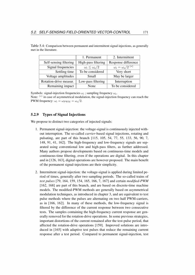
5.2. SELF-SENSING FIELD-ORIENTED VECTOR-CONTROL 171
Table 5.4: Comparison between permanent and intermittent signal injections, as generallymet in the literature.
1. Permanent 2. IntermittentSelf-sensing filtering High-pass filtering Response difference
Signal frequencies ωi ≤ ωs/2 ωi = ωs/2(∗)
Settling time To be considered Very shortVoltage amplitudes Small May be larger
Rotation-drive measur. Low-pass filtering InterruptionRemaining impact None To be considered
Symbols: signal-injection frequencies ωi ; sampling frequency ωs.Note: (∗) in case of asymmetrical modulation, the signal-injection frequency can reach thePWM frequency: ωi = ωPWM = ωs/2.
5.2.9 Types of Signal Injections
We propose to distinct two categories of injected signals:
1. Permanent signal-injection: the voltage-signal is continuously injected with-out interruption. The so-called carrier-based signal injections, rotating andpulsating, are part of this branch [115, 105, 54, 77, 55, 133, 56, 90, 7,148, 91, 41, 162]. The high-frequency and low-frequency signals are sep-arated using conventional low and high-pass filters, as further addressed.Many authors propose developments based on continuous-time models andcontinuous-time filtering, even if the operations are digital. In this chapterand in [126, 163], digital operations are however proposed. The main benefitof the permanent signal-injections are their simplicity.
2. Intermittent signal-injection: the voltage-signal is applied during limited pe-riod of times, generally after two sampling periods. The so-called trains oftest pulses [79, 164, 159, 154, 165, 166, 7, 167] and certain modified-PWM[162, 168] are part of this branch, and are based on discrete-time machinemodels. The modified-PWM methods are generally based on asymmetricalmodulation techniques, as introduced in chapter 3, and are equivalent to testpulse methods where the pulses are alternating on two half PWM-carriers,as in [166, 162]. In many of these methods, the low-frequency signal isfiltered by the difference of the current response between two consecutivetests. The samples containing the high-frequency current response are gen-erally removed for the rotation-drive operations. In some previous strategies,important distortions of the current remained after the test-pulse period, thataffected the rotation-drive operations [159]. Improved solutions are intro-duced in [165] with adaptive test pulses that reduce the remaining currentresponse after a test period. Compared to permanent signal-injection, test

172 CHAPTER 5. SIGNAL PROCESSING
pulses allow to modify the injected voltage after every signal-injection pe-riod and to cover the maximum supplied voltage [165]. The only drawbackconcerns the remaining impact of resistive voltage drops that may affect therotation-drive operations, as explained in [169].
The distinction between permanent and intermittent signal-injections are not al-ways obvious. The method proposed in the next chapter shows that, using discrete-time operations, finite-impulse response filters and some other considerations, bothsignal-injections are quite equivalent. A comparison between the rotating and pul-sating permanent signal-injections is proposed by [66, 120].
Other uses of signal injections
The presence of an anisotropy is not required for double-fed IM. As proposed by[9], the rotor orientation can be deduced from the mutual inductance orientation.This is performed measuring the current response induced in the rotor by high-frequency signals injected in the stator (or inversely).
For information, signal-injection can be performed for other reasons than self-sensing position estimations, but to estimate the motor temperature, based on re-sistance variations during the drive operations, as proposed by [170, 171].
5.2.10 Position Estimation From The Anisotropy Angle
Initial polar ambiguity issue
The angle ϕx is defined on a period π, leading to an inherent ambiguity about thedirections of the poles. Assuming that the orientation of the d-axis is known, thepolar ambiguity can be initially removed by tracking small differences of the in-cremental self-inductance along opposite magnetizing directions: injecting a largetest current along the positive direction of the d-axis should reduce the magneticsaturation in the machine (assuming that ψ
PMis oriented in the direction of nega-
tive values); while injecting a large test current along the negative direction shouldincrease the magnetic saturation in the machine. The incremental self-inductanceshould therefore be slightly larger for positive currents than for negative currentsalong the d-axis. If that difference is larger than the noise, it is possible to removethe initial ambiguity. This strategy is proposed by [79, 164, 95, 172]. It is alsoperformed by [173] for a brushless DC motor, comparing the difference betweenphase inductances with a position look-up table. In [174, 175, 176], large oscillat-ing signals are used instead to test pulses.
Naturally the back-EMF-based self-sensing methods do not have problem ofpolar ambiguity, but are not working at standstill [79]. Combining both anisotropy-based with back-EMF-based self-sensing methods allow to guarantee that the po-larity ambiguity is not lost at higher speeds [177].

5.3. HIGH-FREQUENCY SIGNAL INJECTION 173
Position error due to the load
Misalignment must be corrected if the contribution of the stator current to the mag-netic state becomes significant. This contribution mainly comes from the currentcomponent along the quadratic q-axis, also called load current due to the relation-ship with the torque. Publications propose to compensate for this misalignmentuse look-up tables of angle corrections. These look-up tables however require ini-tial and offline commissioning that are not always feasible in practice. Other re-cent methods combine simultaneously anisotropy-based and back-EMF-based self-sensing methods, in order to compensate for their respective error sources. Assum-ing that the back-EMF estimation is less sensitive to the load current, it can be usedas an online commissioning of the anisotropy misalignment. The angle correctioncan then be performed online. These solutions are proposed in [57, 115, 167, 177].
Position error due to harmonics
A compensation method to the second harmonics in the anisotropy is proposed in[158]. This second harmonic is estimated during a commissioning, but not online.Methods of estimation based on feedback gains are proposed by [53, 56].
5.3 High-Frequency Signal Injection
We propose here the development of the required discrete-time model, the prin-ciple and the conditions for anisotropy-based self-sensing operations using high-frequency signal injections.
5.3.1 The Discrete-Time Model
We assume that the different operations are performed by digital controllers. Adiscretized model is therefore required. The current measurements are sampledwith a frequency νs at instants t[k] = kTs, where Ts = 1/νs is the sampling period.For convenience, the pulse-width modulated signal (PWM) driving the voltage-source inverter (VSI) is synchronized with the sampling times. The mean value ofthe voltage supplied by the VSI between two sampling times was defined in (3.55)as follows:
v[k] ,1
Ts
∫ t[k]
t[k−1]
v(t)dt (5.18)
Assuming that the inverter nonlinearities are compensated, as described in chap-ter 4, the mean voltage supplied by the VSI should be equal to the command voltagesent to the PWM-VSI. Similarly, e[k]
PM is therefore the mean value of the back-EMFbetween two sampling times. The backward-difference of the current was definedin (3.57) as follows:
δi[k] , i(t[k])− i(t[k−1]) (5.19)

174 CHAPTER 5. SIGNAL PROCESSING
And finally the sampling average of the current was defined in (3.58) as follows:
i[k] ,
i(t[k]) + i(t[k−1])
2(5.20)
Base on (5.13) and assuming constant parameters during the sampling periods,the discrete-time machine model without eddy currents in the stationary αβ-frameyields: (
lt+
Tsδi[k] + r+i
[k])
+
(lt-
Tsδi[k] + r-i
[k])∗
ej2ϕx = u[k] (5.21)
where we defined u , v − ePM.
5.3.2 The z-Transform of the Model
The operations can be described using the z-transform of the discrete-time model(5.21). In this chapter, the z-transform of a discrete-time space vector is written:
X(z) , Zx (5.22)
where X is therefore a function of the parameter z. This X should not be confusedwith the matrix space vector introduced in Chapter 3, but not used here. Being usedin the model, the z-transform of the conjugate value x∗ is [46]:
Zx∗ = X∗(z∗) (5.23)
Assume in first approximation that ϕx is constant. Introducing the following z-transform U(z) , Zu, δI(z) , Zδi and I(z) , Zi, the z-transform of themodel (5.21) yields:(
lt+
TsδI(z) + r+I(z)
)+
(lt-
TsδI∗(z∗) + r-I
∗(z∗)
)ej2ϕx = U(z) (5.24)
This expression can be further simplified using the relation between δi and i thatis deduced from (5.19) and (5.20). It can be shown that the relation between theirz-transforms is linked by a transfer function D(z):
δI(z) = D(z)I(z) ⇒ D(z) ,2(1− z−1)
1 + z−1(5.25)
Observe thatD∗(z∗) = D(z). This relation allows to highlight the relation betweenU(z) and either 1) only δI(z) or only 2) I(z) in (5.24), removing the other value.Most of the permanent signal-injection strategies are based on the choice 2) whilemost of the intermittent signal-injection strategies are based on the choice 1). Thisis choice is further addressed. We propose here to continue with the choice 1), and(5.24) can be written:
Z+(z)δI(z) + Z-(z)ej2ϕxδI∗(z∗) = U(z) (5.26)

5.3. HIGH-FREQUENCY SIGNAL INJECTION 175
where we define two transfer-functions Z+(z) and Z-(z), that we respectively callpositive and negative integral-impedances:
Z+(z) =lt+
Ts+
r+
D(z)
Z-(z) =lt-
Ts+
r-
D(z)
(5.27)
In most of the drives, the voltage is the commanded input signal and the current isthe measured output signal. It is therefore required to reverse the relation (5.26).As demonstrated in the annexes of [163] and hereafter, using some mathematicalmanipulations, it is shown that it can be written:
Y+(z)U(z) + Y-(z)ej2ϕxU∗(z∗) = δI(z) (5.28)
where we introduced two transfer-functions Y+(z) and Y-(z), that we respectivelycall positive and negative derivative-admittances, and that are computed as follows:
Y+(z) ,Z+(z)
Zx(z)Zy(z)
Y-(z) , − Z-(z)
Zx(z)Zy(z)
(5.29)
Note that Zx = Z+ + Z- and Zy = Z+ − Z- denote the integral-impedances alongthe xy-axes.
Demonstration of the inversion
It can be shown in (5.27) that Z∗+(z∗) = Z+(z) and Z∗- (z∗) = Z-(z). Using thecomplex conjugate of (5.26) yields:
δI∗(z∗) =(U∗(z∗)− Z-(z)e−j2ϕxδI(z)
)/Z+(z) (5.30)
Replacing δI∗(z∗) back in (5.26) yields:
Z+(z))U(z) =(Z2
+(z)− Z2- (z)
)δI(z) + Z-(z)ej2ϕxU
∗(z∗) (5.31)
Since Z2+(z)− Z2
- (z) = Zx(z)Zy(z), we obtain:
Z+(z)
Zx(z)Zy(z)U(z)− Z-(z)
Zx(z)Zy(z)ej2ϕxU
∗(z∗) = δI(z) (5.32)
5.3.3 The Fourier-Transform of the Model
The signal injection is based on repetitive voltage sequences, generally at fixedfrequencies. It is therefore convenient to use the discrete-time Fourier-transform(DTFT) of the space vector signals that is found replacing z by a unitary complex

176 CHAPTER 5. SIGNAL PROCESSING
value ejωTs in the relations, where ω ≤ ωs/2 = π/Ts. It is shown thatD(z) definedin (5.25) yields:
D(ejωTs) =2(1− e−jωTs)
1 + e−jωTs=
2(ejωTs/2 − e−jωTs/2)
ejωTs/2 + e−jωTs/2= 2
sin(ωTs/2)
cos(ωTs/2)(5.33)
It can also be written as follows:
D(ejωTs) = jωTs where ω ,2
Tstan(ω
Ts
2) (5.34)
with ω that tends to ω when ω ωs. Introducing (5.34) in (5.27) yields the DTFTof the positive and negative integral-impedances:
Z+(z) =lt+
Ts− j r+
ω
Z-(z) =lt-
Ts− j r-
ω
(5.35)
Combining (5.29) with (5.35) yields the DTFT of the positive and negative derivative-admittances:
Y+(ejωTs) = Tslt+ − jr+/ω
(ltx − jrx/ω) (lty − jry/ω)
Y-(ejωTs) = −Ts
lt- − jr-/ω
(ltx − jrx/ω) (lty − jry/ω)
(5.36)
The resistance is often neglected in self-sensing operations and these parametersbecome very simple as the imaginary and frequency dependency vanish:
rx ωltxry ωlty
⇒
Z+(z) =
lt+
Ts
Z-(z) =lt-
Ts
and
Y+ = Ts
lt+
ltxlty
Y- = −Tslt-
ltxlty
(5.37)
Let us define the inverse incremental self-inductances as follows: ytx , l−1tx and
yty , l−1ty . The derivative-admittances therefore yields:
Y+ = Ts
lt+
ltxlty=Ts
2
ltx + ltyltxlty
=Ts
2(yty + ytx) = Tsyt+
Y- = Tslt-
ltxlty=Ts
2
ltx − ltyltxlty
=Ts
2(yty − ytx) = Tsyt-
(5.38)
This is a common formalism found in some publications.

5.3. HIGH-FREQUENCY SIGNAL INJECTION 177
M
rotation-drive op.
PWMVSI
self-sensingoperations
Filter
i
ic
vc
v
rotation-drive plant
vi
ϕx
Figure 5.1: Flowchart of the rotation-drive plant including a signal-injection and a self-sensing computation
5.3.4 Principle and Assumptions
The principle is illustrated in Figure 5.1. It consists in the injection of a high-frequency voltage, written vi and computed by the self-sensing operations, in ad-dition to the low-frequency voltage, written vc and computed by the rotation-driveoperations: v = vc + vi. As a consequence, a high-frequency current response iiis added to the low-frequency current response ic controlled by the rotation-driveoperations: i = ic + ii.
In order to prevent or reduce disturbing interactions, the signal-injection op-erations and the rotation-drive operations should produce signals xi and xc cov-ering separated frequency ranges ωc and ωi respectively. In terms of DTFTX = Fx, the condition is:
|Xc(ω)| |X i(ω)| for ω ∈ ωi|Xc(ω)| |X i(ω)| for ω ∈ ωc
(5.39)
Obviously, higher the signal-injection frequency, better is the separation [162, 147].Note that the frequency content of the PWM is not considered in discrete-timeoperations and is, by consequence, excluded from the condition (5.39).
The high-frequency signals inevitably produce a high-frequency torque leadingto high-frequency vibrations (that are audible under 20 kHz) and, by consequence,to a high-frequency back-EMF. The mechanical damping effects (due to the inertiaplus the frictions of the machine and the coupled load) tend however to increasewith the frequency, reducing the high-frequency back-EMF to a negligible value.In terms of DTFT of the back-EMF EPM = FePM and of the PWM meanvoltage V = Fv, this leads to:∣∣∣EPM(ω)
∣∣∣ ∣∣∣V (ω)∣∣∣ for ω ∈ ωi (5.40)
The back-EMF can therefore be removed from the high-frequency electrical modeland from self-sensing operations such that U i(ω) ≈ V i(ω). Introducing theseassumptions (5.39) and (5.40), the relation (5.28) yields for the injected signals:
Y+(ejωTs)V i(ejωTs) + Y-(e
jωTs)ej2ϕx V∗i (e−jωTs) = δI i(e
jωTs) (5.41)
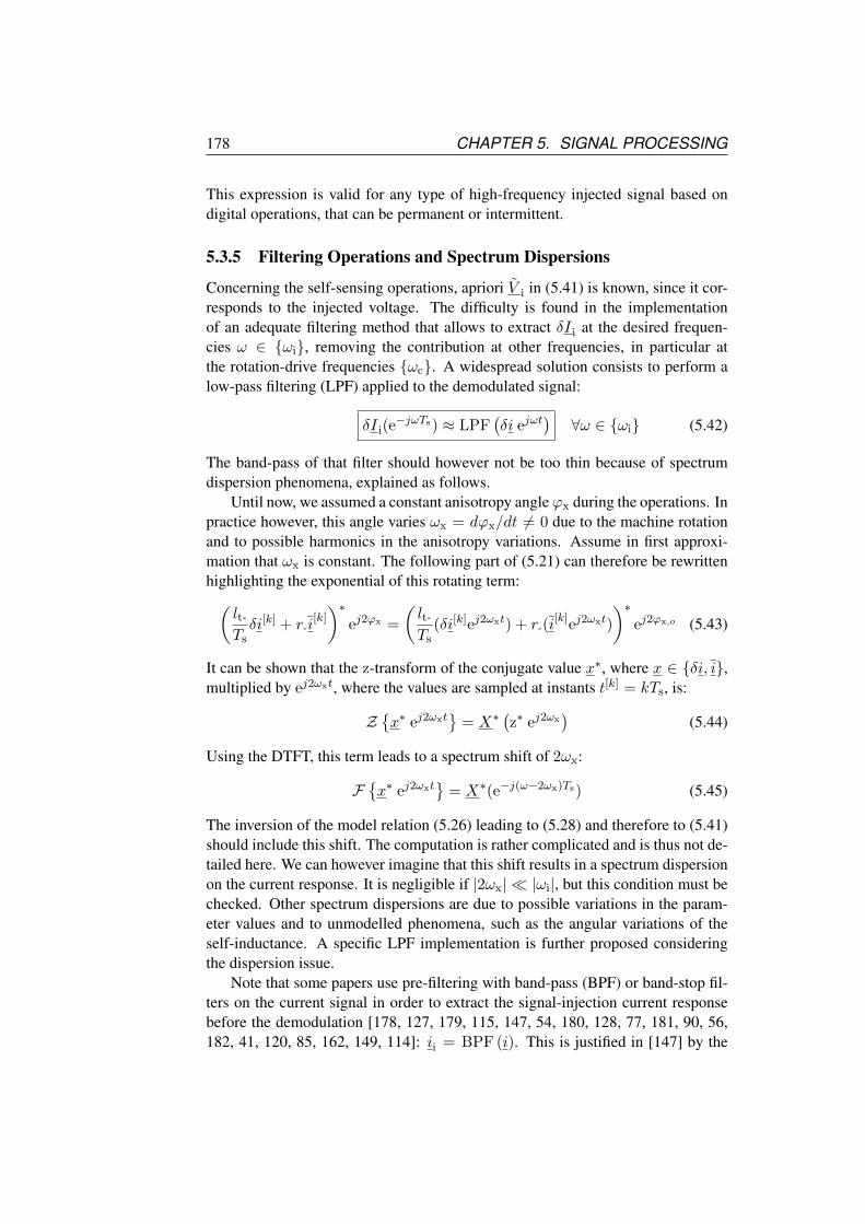
178 CHAPTER 5. SIGNAL PROCESSING
This expression is valid for any type of high-frequency injected signal based ondigital operations, that can be permanent or intermittent.
5.3.5 Filtering Operations and Spectrum Dispersions
Concerning the self-sensing operations, apriori V i in (5.41) is known, since it cor-responds to the injected voltage. The difficulty is found in the implementationof an adequate filtering method that allows to extract δI i at the desired frequen-cies ω ∈ ωi, removing the contribution at other frequencies, in particular atthe rotation-drive frequencies ωc. A widespread solution consists to perform alow-pass filtering (LPF) applied to the demodulated signal:
δI i(e−jωTs) ≈ LPF
(δi ejωt
)∀ω ∈ ωi (5.42)
The band-pass of that filter should however not be too thin because of spectrumdispersion phenomena, explained as follows.
Until now, we assumed a constant anisotropy angleϕx during the operations. Inpractice however, this angle varies ωx = dϕx/dt 6= 0 due to the machine rotationand to possible harmonics in the anisotropy variations. Assume in first approxi-mation that ωx is constant. The following part of (5.21) can therefore be rewrittenhighlighting the exponential of this rotating term:(
lt-
Tsδi[k] + r-i
[k])∗
ej2ϕx =
(lt-
Ts(δi[k]ej2ωxt) + r-(i
[k]ej2ωxt)
)∗ej2ϕx,o (5.43)
It can be shown that the z-transform of the conjugate value x∗, where x ∈ δi, i,multiplied by ej2ωxt, where the values are sampled at instants t[k] = kTs, is:
Zx∗ ej2ωxt
= X∗
(z∗ ej2ωx
)(5.44)
Using the DTFT, this term leads to a spectrum shift of 2ωx:
Fx∗ ej2ωxt
= X∗(e−j(ω−2ωx)Ts) (5.45)
The inversion of the model relation (5.26) leading to (5.28) and therefore to (5.41)should include this shift. The computation is rather complicated and is thus not de-tailed here. We can however imagine that this shift results in a spectrum dispersionon the current response. It is negligible if |2ωx| |ωi|, but this condition must bechecked. Other spectrum dispersions are due to possible variations in the param-eter values and to unmodelled phenomena, such as the angular variations of theself-inductance. A specific LPF implementation is further proposed consideringthe dispersion issue.
Note that some papers use pre-filtering with band-pass (BPF) or band-stop fil-ters on the current signal in order to extract the signal-injection current responsebefore the demodulation [178, 127, 179, 115, 147, 54, 180, 128, 77, 181, 90, 56,182, 41, 120, 85, 162, 149, 114]: ii = BPF (i). This is justified in [147] by the

5.3. HIGH-FREQUENCY SIGNAL INJECTION 179
N = 3
N = 12
−ω
1
0.8
0.6
0.4
0.2
0−ωs/3−ωs/2 −ωs/10 −ωs/100
−ωi
ωc
Figure 5.2: Filtering characteristics (magnitudes) of the moving average (dashed line) andthe moving average shifted at ωs/3 (plain line) for N = 3 and N = 12, as a function ofthe signal frequency.
use of analog measurements that requires a notch filter in order to reject harmonicsof the PWM frequency. But it is not required if the sampling is synchronized withthe PWM. This is also not required since (5.53) naturally removes the frequencycontent outside −ωi. Moreover, the fact to use operations directly based on the ra-tio between the current and the high-frequency voltage removes lagging problems[128, 54, 183]. No prefiltering is performed by [105, 133].
5.3.6 Filter Implementation
We propose LPF operations based on the moving average, that is a finite impulseresponse (FIR) filter defined as the mean of the N previous discrete-time values x,computed every sampling period k [46]:
LPF[k]N (x) :=
1
N
N−1∑n=0
x[k−n] (5.46)
Its characteristic for the negative frequencies is illustrated in Figure 5.2 with dashedlines for the case N = 3 and N = 12. Note that the characteristic is symmetricalaround zero. Assume that the considered high-frequency ωi of the injected signalsis an integer fraction Ni ≥ 3 of the sampling frequency ωs:
ωi = ωs/Ni ⇒ ωiTs = 2π/Ni (5.47)
The moving average (5.46) can then be used as a LPF for the operation (5.42)computed at −ωi, selecting an integer multiple N of Ni:
δI i(e−jωiTs) ≈ 1
N
N−1∑n=0
(δi[k−n] ej2π(k−n)/Ni
)(5.48)
Considering the case Ni = 3, the characteristic of the moving averages shiftedaround −ωi = −ωs/3 is illustrated in Figure 5.2 with plain lines for N = Ni = 3and N = 4 × Ni = 12. The choice of N depends on the expanse of the low-frequency range ωc to be removed. However, assuming that ωi is much higher
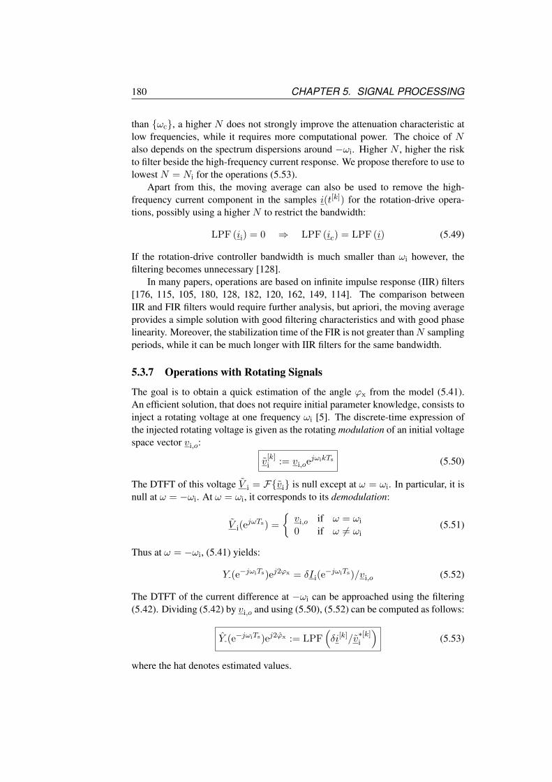
180 CHAPTER 5. SIGNAL PROCESSING
than ωc, a higher N does not strongly improve the attenuation characteristic atlow frequencies, while it requires more computational power. The choice of Nalso depends on the spectrum dispersions around −ωi. Higher N , higher the riskto filter beside the high-frequency current response. We propose therefore to use tolowest N = Ni for the operations (5.53).
Apart from this, the moving average can also be used to remove the high-frequency current component in the samples i(t[k]) for the rotation-drive opera-tions, possibly using a higher N to restrict the bandwidth:
LPF (ii) = 0 ⇒ LPF (ic) = LPF (i) (5.49)
If the rotation-drive controller bandwidth is much smaller than ωi however, thefiltering becomes unnecessary [128].
In many papers, operations are based on infinite impulse response (IIR) filters[176, 115, 105, 180, 128, 182, 120, 162, 149, 114]. The comparison betweenIIR and FIR filters would require further analysis, but apriori, the moving averageprovides a simple solution with good filtering characteristics and with good phaselinearity. Moreover, the stabilization time of the FIR is not greater thanN samplingperiods, while it can be much longer with IIR filters for the same bandwidth.
5.3.7 Operations with Rotating Signals
The goal is to obtain a quick estimation of the angle ϕx from the model (5.41).An efficient solution, that does not require initial parameter knowledge, consists toinject a rotating voltage at one frequency ωi [5]. The discrete-time expression ofthe injected rotating voltage is given as the rotating modulation of an initial voltagespace vector vi,o:
v[k]i := vi,oe
jωikTs (5.50)
The DTFT of this voltage V i = Fvi is null except at ω = ωi. In particular, it isnull at ω = −ωi. At ω = ωi, it corresponds to its demodulation:
V i(ejωTs) =
vi,o if ω = ωi
0 if ω 6= ωi(5.51)
Thus at ω = −ωi, (5.41) yields:
Y-(e−jωiTs)ej2ϕx = δI i(e
−jωiTs)/vi,o (5.52)
The DTFT of the current difference at −ωi can be approached using the filtering(5.42). Dividing (5.42) by vi,o and using (5.50), (5.52) can be computed as follows:
Y-(e−jωiTs)ej2ϕx := LPF
(δi[k]/v
∗[k]i
)(5.53)
where the hat denotes estimated values.

5.3. HIGH-FREQUENCY SIGNAL INJECTION 181
0.05ωs/20 ωs/15 ωs/5ωs/10 ωs/3 ωs
0.10
0.15
ωi
88
90
98
56
60
66
r x(Ω
)l t,x
(µH
)r y
(Ω)
l t,x
(µH
)
Figure 5.3: Apparent resistances and inductances of the experimental BLDC machineidentified at different frequencies ωi, assuming νs = 10 kHz, with ωs = 2πνs.
Position Estimation
As it is widely assumed in the literature, if the resistance impact is negligible com-pared to the inductance, the positive Y+ and negative Y- derivative-admittances arestrictly real values: (5.37). Using (5.53), the angle is then easily extracted by:
ϕx :=∠ (−LPF (δi/v∗i ))
2(5.54)
where ∠ denotes the complex argument. The minus in front of−LPF(·) is requiredbecause Y- < 0. In practice however, the resistance is not always negligible, andY- is not strictly real, leading to angle estimation errors. Using (5.54), this error isthe half complex argument of Y- given in (5.36):
ϕx|(5.54) − ϕx =∠(−Y-(e
−jωiTs))
2
=∠ (lt- + jr-/ωi)− ∠ (ltx + jrx/ωi)− ∠ (lty + jry/ωi)
2(5.55)
Note here that higher ωi, lower the impact of the resistance. Except in [184, 90,185, 183, 91, 148, 85, 149], the resistance impact is often neglected in signal-injection operations using rotating signal injections. This position error is ad-dressed in [54, 90]. It is analyzed hereafter for experimental cases.
Experimental Cases
Figure 5.3 shows the apparent parameters of the experimental BLDC motor for dif-ferent pulsating-signal frequencies along the x and y-axes, and with νs = 10 kHz.These values are also in Figure 3.12 of chapter 3. Figure 5.4 shows the theoreti-cal error due to the resistance, and computed using (5.55). The circles, joined by
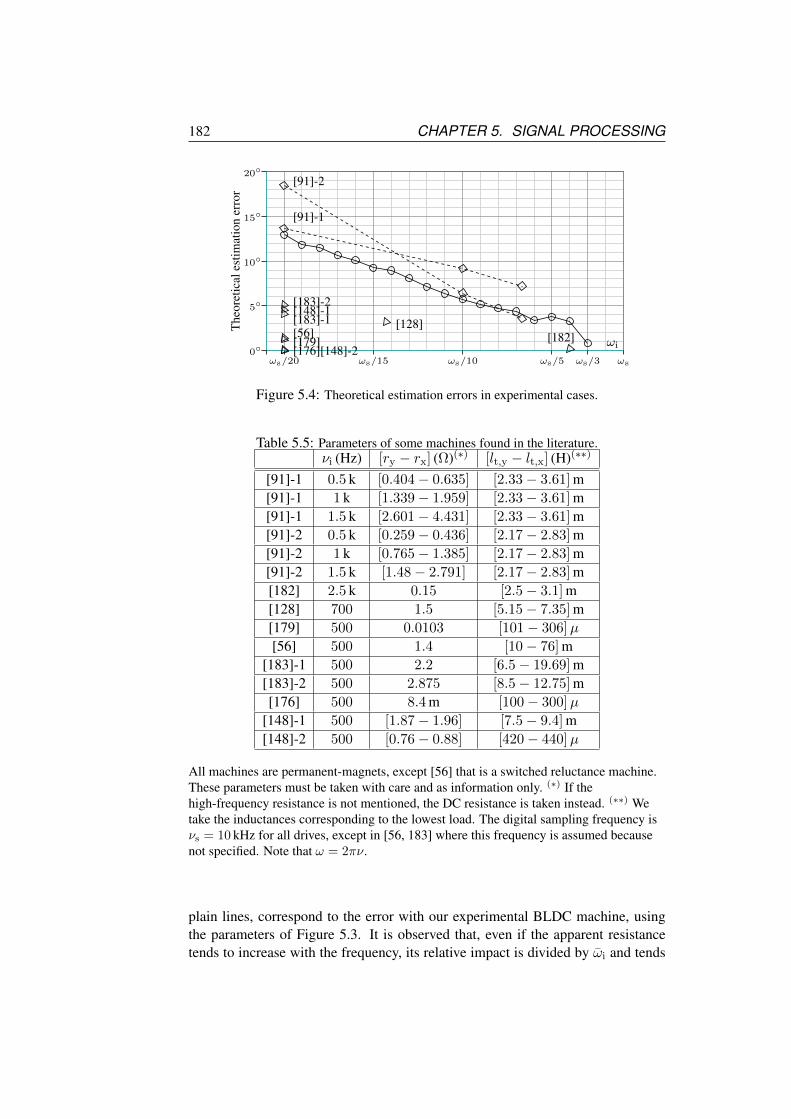
182 CHAPTER 5. SIGNAL PROCESSING
[182][128]
[179][56][176][148]-2
[183]-2[183]-1[148]-1
[91]-2
[91]-1
ωs/20 ωs/15 ωs/5ωs/10 ωs/3 ωs
ωi
20
15
10
5
The
oret
ical
estim
atio
ner
ror
0
Figure 5.4: Theoretical estimation errors in experimental cases.
Table 5.5: Parameters of some machines found in the literature.νi (Hz) [ry − rx] (Ω)(∗) [lt,y − lt,x] (H)(∗∗)
[91]-1 0.5 k [0.404− 0.635] [2.33− 3.61] m[91]-1 1 k [1.339− 1.959] [2.33− 3.61] m[91]-1 1.5 k [2.601− 4.431] [2.33− 3.61] m[91]-2 0.5 k [0.259− 0.436] [2.17− 2.83] m[91]-2 1 k [0.765− 1.385] [2.17− 2.83] m[91]-2 1.5 k [1.48− 2.791] [2.17− 2.83] m[182] 2.5 k 0.15 [2.5− 3.1] m[128] 700 1.5 [5.15− 7.35] m[179] 500 0.0103 [101− 306]µ
[56] 500 1.4 [10− 76] m[183]-1 500 2.2 [6.5− 19.69] m[183]-2 500 2.875 [8.5− 12.75] m[176] 500 8.4 m [100− 300]µ
[148]-1 500 [1.87− 1.96] [7.5− 9.4] m[148]-2 500 [0.76− 0.88] [420− 440]µ
All machines are permanent-magnets, except [56] that is a switched reluctance machine.These parameters must be taken with care and as information only. (∗) If thehigh-frequency resistance is not mentioned, the DC resistance is taken instead. (∗∗) Wetake the inductances corresponding to the lowest load. The digital sampling frequency isνs = 10 kHz for all drives, except in [56, 183] where this frequency is assumed becausenot specified. Note that ω = 2πν.
plain lines, correspond to the error with our experimental BLDC machine, usingthe parameters of Figure 5.3. It is observed that, even if the apparent resistancetends to increase with the frequency, its relative impact is divided by ωi and tends

5.3. HIGH-FREQUENCY SIGNAL INJECTION 183
to decrease. This tends to confirm the benefits of using the highest frequency.Results using the parameters of some machines found in the literature are
shown by diamonds and triangles. The parameters can be found in Table 5.5. Ifthere is more than one machine in one reference, the reference is followed by anumbering for each machine. In [91], parameters of two machines are given atthree different frequencies. The corresponding errors are mentioned in Figure 5.4by diamonds joined by dashed lines. A decrease of the resistance impact is alsoobserved. The other machines are mentioned by triangles. We can see that manypapers chose a frequency at νi = νs/20 = 500 Hz. Even if the error is typicallynot much larger than 5, using higher frequencies could possibly further reduce theresistance impact.
5.3.8 Operations with Pulsating Signals
Another possibility to obtain an estimation of the angle ϕx from the model (5.41)consists to inject a pulsating voltage at one frequency ωi [5]. The initial param-eter knowledge must however be discussed. The discrete-time expression of theinjected pulsating voltage can be given as the sum of two voltage space vectorsrotating in opposition with respect to an fixed voltage vi,o:
v[k]i := vi,o
ejωikTs + e−jωikTs
2= vi,o cos(ωikTs) (5.56)
The voltage vi,o has a fixed amplitude Vi and is oriented by an angle ϕi that maypossibly vary at a lower frequency than ωi, around ωc:
vi,o := Viejϕi (5.57)
The DTFT of this voltage V i = Fvi is null except at ω = ±ωi and yields in thecase ωi < ωs/2:
V i(ejωTs) =
vi,o/2 if ω = ±ωi
0 if ω 6= ωi(5.58)
Due to this spectrum content, not null at two opposite frequencies, it is not possibleto isolate the negative part of the relation (5.41) as done previously with rotatingsignals. But other strategies are possible using the property of V i being equal atω = ±ωi. We propose to sum the relation (5.41) at ω = ωi and at ω = −ωi. Since:
Y±(e−jωiTs) = Y ∗± (ejωiTs) ⇒ Y±(ejωiTs) + Y±(e−jωiTs)
2= <
(Y±(ejωiTs)
)(5.59)
And since v∗i,o = vi,oe−2jϕi , it can be shown that it yields:
<(Y+(ejωiTs)
)+ <
(Y-(e
jωiTs))
ej2(ϕx−ϕi) =δI i(e
jωiTs) + δI i(e−jωiTs)
vi,o
(5.60)

184 CHAPTER 5. SIGNAL PROCESSING
(II)
(a) (b)
(I)
= <(Yy) <(Yx)
<(Y+) <(Y+)<
= <(Yy) <(Yx)
<<(Y+)
−π2
π2
−π2
ϕx − ϕi
ϕx − ϕiπ2
<(Y-)ej2(ϕx−ϕi)<(Y-)e
j2(ϕx−ϕi)
<(Y-)ej2(ϕx−ϕi)<(Y-)e
j2(ϕx−ϕi)
−π2
π2
−π2
ϕx − ϕi
ϕx − ϕiπ2
Figure 5.5: Illustration of (a) the approached locus of <(Y-)ej2(ϕx−ϕi) compared to the
correct one <(Y-)ej2(ϕx−ϕi) assuming a faulty <(Y+) ; and (b) approached angle between
the anisotropy and the signal-injection ϕx − ϕi as a function of the correct one ϕx − ϕi.Case (I): <(Y+) < <(Y+) ; Case (II): <(Y+) > <(Y+).
The sum of DTFT of the current difference at the two frequencies can be ap-proached using the filtering (5.42). Dividing by vi,o, using (5.56) and (5.57), ityields:
δI i(ejωiTs) + δI i(e
−jωiTs)
vi,o
≈LPF
(δi (ejωit + e−jωit)
)vi,o
=LPF (δi 2 cos(ωit))
vi,o
=LPF
(δi cos(ωit) v
∗i,o
)vi,o v
∗i,o /2
=LPF (δi v∗i )
V 2i /2
(5.61)
⇒ <(Y+(ejωiTs)
)+ <
(Y-(e
jωiTs))
ej2(ϕx−ϕi) :=LPF (δi v∗i )
V 2i /2
(5.62)
where the hat denotes estimated values.
Position Estimation
In the case of a permanent signal, the possibilities to modify the angleϕi are limitedto slow variations, in order to limit the effect on spectrum dispersion, as previouslydiscussed. A strategy, largely found in the literature, consists to track the anisotropyangle: ϕi → ϕx. A shift between these angles leads to an estimation error εx
that is used in a regulator (proportional-integral for instance) that computes theanisotropy angle estimation: ϕx = REG(εx). Two possible computations of theestimation error are addressed hereafter. Note that there is a settling time relatedto the initially tracking of the anisotropy angle. This time depends on the regulator

5.3. HIGH-FREQUENCY SIGNAL INJECTION 185
bandwidth (or regulation poles) that is limited by the signal-injection period. Byconsequence, higher the signal-injection frequency, lower the minimum settlingtime. This settling time (in addition to settling times due to the noise filtering anddue to any compensation method) is a drawback that does not exist in other self-sensing methods. Note that strategies using ϕi → ϕy are also valid and result insimilar operations.
1. Either the estimation error is computed taking the imaginary part of (5.62):
εx :== (LPF (δi v∗i ))
<(Y-(ejωiTs)
)V 2
i
(5.63)
This method is found in [186, 184, 59, 133, 68, 41, 85, 149, 114].
2. Or the estimation error is computed taking the angle of (5.62) reduced by thepositive derivative-admittance estimation:
εx := ∠
(−LPF (δi v∗i )
V 2i /2
+ <(Y+(ejωiTs)
))/2 (5.64)
Both methods require at least an approximate knowledge of one parameter. Forthe method 1. it is: Y- ; and for the method 2. it is: Y+. These methods aretherefore not really parameter independent. Figure 5.5(a) illustrates the error onthe angle estimation ϕx consequent to an error on <(Y+) with respect to <(Y+)using (5.64). As illustrated in Figure 5.5(b), the impact of this error should vanishwhile ϕi → ϕx. It is therefore not required to have an accurate knowledge of<(Y+), but the only requirement is: <(Yy) < <(Y+) < <(Yx). This is discussed in[126].
5.3.9 Operations with Alternating Signals
The operations (5.62) are simplified to their maximum with the case of an signalinjected at half the sampling frequency: ωi = ωs/2. Using (5.47), it correspondsto Ni = 2 and vi is purely alternating after every sampling period, as illustrated inFigure 5.6:
v[k]i := vi,o ejπk = (−1)k vi,o (5.65)
This alternating signal can be handled as a pulsating signal, but the relation presentssome differences that should be considered. The DTFT of this voltage differs com-pared to (5.58) due to frequency overlays:
V i(ejωTs) =
vi,o if ω = ±ωi = ±ωs/2
0 if ω 6= ±ωi(5.66)

186 CHAPTER 5. SIGNAL PROCESSING
Ts
t
t[k] = kTs
v
i0
0
v[k]i
v[k]c
i(t[k])
i[k]c = i[k]
δi[k]
Figure 5.6: Illustration of the alternating signal-injection in addition to the rotation-driveoperating signals (along ejϕi ). The dots correspond to the current samples used for self-sensing operations. The circles correspond to the current value used as input for therotation-drive control.
At the injected frequencies, using (5.34) we can compute that ωi = ∞ and thecondition to obtain (5.38) is met: Y± = Tsyt±. The filtering operations (5.46)are reduced to two sampling periods, i.e. three samples i(t), (including the initial,middle and last sample), such that (5.61) yields:
LPF[k]N=2 (δi 2 cos(πk)) = δi[k]−δi[k−1] = i(t[k])−2i(t[k−1])+ i(t[k−2]) (5.67)
The current back-differences are illustrated in Figure 5.6. Following the same stepsas for the previous pulsating signal development, it yields:
yt+ − yt-ej2(ϕx−ϕi) :=
i(t[k])− 2i(t[k−1]) + i(t[k−2])
2 v[k]i Ts
(5.68)
An equivalent form of this operation was proposed in [126].Since ωi = ∞, the signal-injection contribution to the current sample-average
is null: ii = 0. Therefore, the LPF operation (5.49) applied on the signal for therotation-drive input can be reduced to only one sampling period, and it correspondsto:
i[k]c := LPF
[k]N=2 (i) =
i(t[k]) + i(t[k−1])
2= i
[k] (5.69)
This value is illustrated by circles in Figure 5.6.
Position Estimation For Permanent Signals
The strategy differs if we use a permanent or an intermittent signal. The case ofthe intermittent signal is further discussed.

5.3. HIGH-FREQUENCY SIGNAL INJECTION 187
1. In the case of a permanent alternating signal, the operation (5.63) combinedwith (5.68) yields:
εx := −=
(i(t[k])− 2i(t[k−1]) + i(t[k−2])
v[k]i yt- Ts
)(5.70)
where an approximate knowledge of yt- is required. This solution seems tobe used by some authors [178, 181, 182]. However, all the developmentsare given under the form of continuous-time operations, leading to someinterrogations about the filtering operations.
2. The operation (5.64) combined with (5.68) yields:
εx := ∠
(− i(t
[k])− 2i(t[k−1]) + i(t[k−2])
2 v[k]i Ts
+ yt+
)/2 (5.71)
where an approximate knowledge of yt+ is required. This second methodwas proposed in [126].
The choice of method 2. for the experiments on the BLDC motor in [126] wasjustified by the significant harmonics in the machine anisotropy, described in chap-ter 2. These harmonics produce strong variations of yt- during the rotation, whileyt+ was more stable, justifying the choice.
Position Estimation For Test Pulses
In the case of an intermittent signal, such as test pulses, the angle ϕi is easilychanged after every test. The test pulses can be treated as alternating pulsatingsignals. Injection the test voltage at least following two different angles, denotedby I and II, and assuming that the anisotropy angle ϕx did not significantly changebetween the two tests, it can be estimated by subtraction the two results (5.68) asfollows:
yt-ej2ϕx =
Eq.(5.68)I − Eq.(5.68)II
e−j2ϕi,II − e−j2ϕi,I(5.72)
Since yt- is strictly real and positive, the angle is found taking the complex argu-ment ∠ of (5.72):
ϕx := ∠
(Eq.(5.68)I − Eq.(5.68)II
e−j2ϕi,II − e−j2ϕi,I
)/2 (5.73)
This is the solution proposed by [165], that is greatly simplified using quadraticsignal injections. Note first of all that there is no angular error due to the resistance.The resistance can however lead to a remaining impact of the signal injection afterthe test period, that can disturb the rotation-drive operations. This problem wasaddressed in [169], however the solution was not perfect.
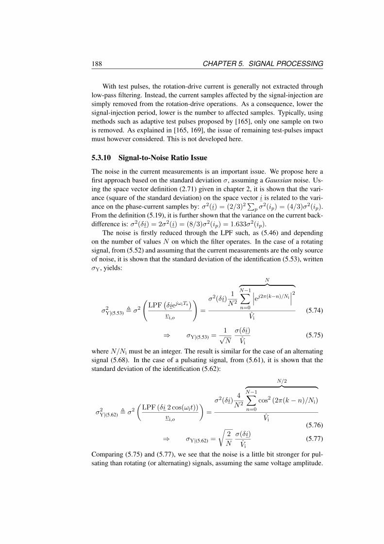
188 CHAPTER 5. SIGNAL PROCESSING
With test pulses, the rotation-drive current is generally not extracted throughlow-pass filtering. Instead, the current samples affected by the signal-injection aresimply removed from the rotation-drive operations. As a consequence, lower thesignal-injection period, lower is the number to affected samples. Typically, usingmethods such as adaptive test pulses proposed by [165], only one sample on twois removed. As explained in [165, 169], the issue of remaining test-pulses impactmust however considered. This is not developed here.
5.3.10 Signal-to-Noise Ratio Issue
The noise in the current measurements is an important issue. We propose here afirst approach based on the standard deviation σ, assuming a Gaussian noise. Us-ing the space vector definition (2.71) given in chapter 2, it is shown that the vari-ance (square of the standard deviation) on the space vector i is related to the vari-ance on the phase-current samples by: σ2(i) = (2/3)2
∑p σ
2(ip) = (4/3)σ2(ip).From the definition (5.19), it is further shown that the variance on the current back-difference is: σ2(δi) = 2σ2(i) = (8/3)σ2(ip) = 1.633σ2(ip).
The noise is firstly reduced through the LPF such, as (5.46) and dependingon the number of values N on which the filter operates. In the case of a rotatingsignal, from (5.52) and assuming that the current measurements are the only sourceof noise, it is shown that the standard deviation of the identification (5.53), writtenσY, yields:
σ2Y|(5.53) , σ2
(LPF
(δiejωiTs
)vi,o
)=
σ2(δi)1
N2
N︷ ︸︸ ︷N−1∑n=0
∣∣∣ej2π(k−n)/Ni
∣∣∣2Vi
(5.74)
⇒ σY|(5.53) =1√N
σ(δi)
Vi
(5.75)
where N/Ni must be an integer. The result is similar for the case of an alternatingsignal (5.68). In the case of a pulsating signal, from (5.61), it is shown that thestandard deviation of the identification (5.62):
σ2Y|(5.62) , σ2
(LPF (δi 2 cos(ωit))
vi,o
)=
σ2(δi)4
N2
N/2︷ ︸︸ ︷N−1∑n=0
cos2 (2π(k − n)/Ni)
Vi(5.76)
⇒ σY|(5.62) =
√2
N
σ(δi)
Vi
(5.77)
Comparing (5.75) and (5.77), we see that the noise is a little bit stronger for pul-sating than rotating (or alternating) signals, assuming the same voltage amplitude.

5.3. HIGH-FREQUENCY SIGNAL INJECTION 189
In practice, the voltage is not measured, but a noise exists in the PWM signals.The assessment of this noise would require further experiments. It is neglectedhere. In a second time, the remaining noise is inherited by the position estimationϕx through one of the operations (5.54), (5.63), (5.64), (5.70), (5.71) or (5.73).This noise could be further filtered, as done in all the publications. Filtering solu-tions are detailed in [114]. A large description of position/speed/torque observersis addressed in [187] for PM machines.
There is however a limit in the admissible inherited noise due to the nonlinear-ity of the operation of position estimation: if the ratio between inherited noise andthe negative derivative-admittance <(Y-) is higher than 1, then some identificationpoints could lead to π-turn estimation errors. The consequences can be dramaticbecause the polarity of the anisotropy can be lost. We propose therefore to selectthe minimum signal magnitude to be used for signal-injection methods as follows,based on two times σY that should cover 94.5 % of the identification points:
2σY < <(Y-) ⇒
Vi >2√N
σ(δi)
<(Y-)for rotating signals
Vi > 2√
2N
σ(δi)
<(Y-)for pulsating signals
(5.78)
We see that increasing N in the LPF reduce the lower limit of the injected voltage.This consideration however neglect the signal-to-noise on the supplied voltage, thatdecrease with the signal amplitude.
Further analysis of the noise is proposed by [105] from the point of view of totalharmonic distortion (THD). ...Some authors proposed to draw maps of feasibilityregions, representing the limit of the self-sensing accuracy as a function of [58, 59,60]
Experimental example
The issue of the measurements noise is illustrated with experiments performed ona standstill uncoupled machine with PM oriented following ϕd = 120, equiva-lent to ϕq = 30. In that orientation, we have an overlay of the qd-frame and thexy-frame, as developed in chapter 2 and in [92]. The stator current has an ampli-tude of ‖i‖ = 25 A and is oriented along the negative d-axis, i.e. ∠i = −60.This stator current is chosen in order to prevent the effects of the zero-crossinginverter nonlinearities and in order to keep the rotor fixed in the desired position.The sampling frequency is νs = 10 kHz. The identification is performed usingpulsating high-frequency voltages between 5 kHz and 1.25 kHz, i.e. Ni = 2 up to8, oriented along 18 different angles ϕi. There are 201 identification points foreach condition, as shown in Figure 5.7 for the cases Ni = 2 and 8. The voltageamplitudes are adapted depending on the frequency, in order to produce a pulsat-ing high-frequency current response with similar amplitudes. The moving averageused for the LPF computation is based on N = Ni. The results are shown inTable 5.3.10.
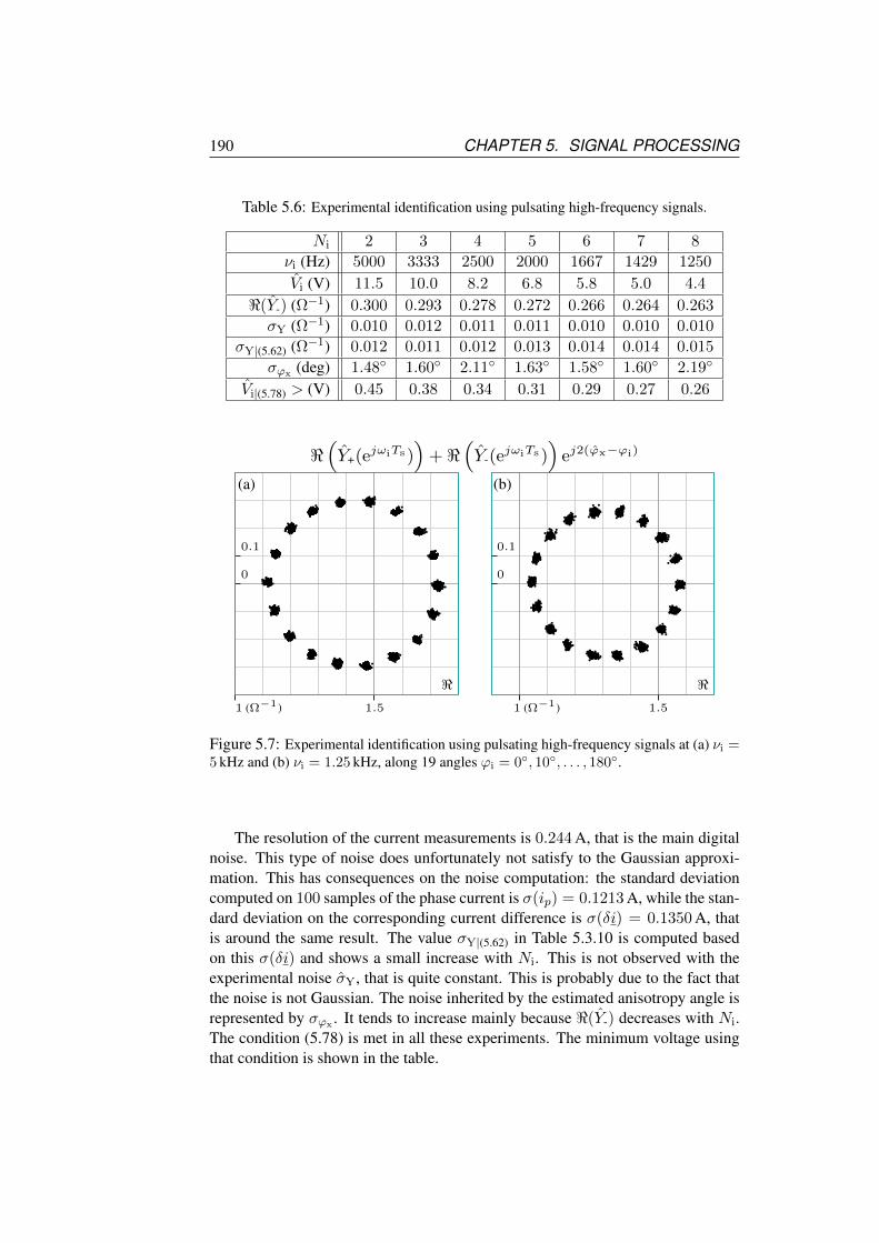
190 CHAPTER 5. SIGNAL PROCESSING
Table 5.6: Experimental identification using pulsating high-frequency signals.
Ni 2 3 4 5 6 7 8
νi (Hz) 5000 3333 2500 2000 1667 1429 1250
Vi (V) 11.5 10.0 8.2 6.8 5.8 5.0 4.4
<(Y-) (Ω−1) 0.300 0.293 0.278 0.272 0.266 0.264 0.263
σY (Ω−1) 0.010 0.012 0.011 0.011 0.010 0.010 0.010
σY|(5.62) (Ω−1) 0.012 0.011 0.012 0.013 0.014 0.014 0.015
σϕx (deg) 1.48 1.60 2.11 1.63 1.58 1.60 2.19
Vi|(5.78) > (V) 0.45 0.38 0.34 0.31 0.29 0.27 0.26
<
0
0.1
1 (Ω−1) 1.5
<1 (Ω−1) 1.5
0
0.1
<(Y+(ejωiTs)
)+ <
(Y-(e
jωiTs))
ej2(ϕx−ϕi)
(a) (b)
Figure 5.7: Experimental identification using pulsating high-frequency signals at (a) νi =5 kHz and (b) νi = 1.25 kHz, along 19 angles ϕi = 0, 10, . . . , 180.
The resolution of the current measurements is 0.244 A, that is the main digitalnoise. This type of noise does unfortunately not satisfy to the Gaussian approxi-mation. This has consequences on the noise computation: the standard deviationcomputed on 100 samples of the phase current is σ(ip) = 0.1213 A, while the stan-dard deviation on the corresponding current difference is σ(δi) = 0.1350 A, thatis around the same result. The value σY|(5.62) in Table 5.3.10 is computed basedon this σ(δi) and shows a small increase with Ni. This is not observed with theexperimental noise σY, that is quite constant. This is probably due to the fact thatthe noise is not Gaussian. The noise inherited by the estimated anisotropy angle isrepresented by σϕx . It tends to increase mainly because <(Y-) decreases with Ni.The condition (5.78) is met in all these experiments. The minimum voltage usingthat condition is shown in the table.

5.3. HIGH-FREQUENCY SIGNAL INJECTION 191
Choice of the current back-difference
In most of the papers dealing with rotating voltage injection, the self-sensing op-erations are based on the current samples instead of the current back-differences.The corresponding relation is simply found replacing the current back-differenceusing the relation (5.25) combined with the definition (5.34):
δI(ejωTs) = jωTs I(ejωTs) (5.79)
Our choice of the current back-differences is however justified as follows. Usingthe definitions (5.20) and (5.19), the standard deviation σ, that corresponds to thenoise, yield:
σ(δi) = 2σ(i) (5.80)
Assume a fixed voltage amplitude |V | for the comparison and assume that the samefiltering method (5.42) would be applied in both cases, it is shown that the signal-to-noise ratio of the current back-differences becomes favorable above:
2 ≤ |ωTs| ⇒ σ(δI(ejωTs)
)≤ |ωTs| σ
(I(ejωTs)
)(5.81)
Using (5.34), it corresponds to: |ωTs| ≥ π/2. At first glance, since the maxi-mum frequency for discrete-time signals is such that |ωmaxTs| = π, this conditionstrongly limit the frequencies at which the use of current back-differences is fa-vorable. It is however further shown that many other benefits are found usinghigh-frequencies in that range [163].
Note that the use of current back-differences is a benefic compared to the useof average current samples in terms of filtering. For the comparison, assume sim-ilar amplitudes for rotating-drive voltages and injected voltages. Using (5.79), wecan say that the amplitude of δic is even reduced by its low frequency content ωc
regarding δii increased by the high-frequency content ωi. This is a strong benefitcompared to operations based on current samples or average current samples.
5.3.11 Issue regarding the PWM-VSI
We assume that the voltages are not measured but the command voltage is usedinstead. Dead-times in the pulse-width modulation (PWM) and voltage drops atthe semiconductors of the voltage-source inverter (VSI) are common nonlinear-ities that must be managed. They can generally be linearized and compensatedassuming fixed phase current flows [5, 121, 41, 114]. This is largely addressed inchapter 4. The frequency content of the compensation signal is mainly present inthe low-frequencies and should therefore not affect the self-sensing operations.
As explained in chapter 4, when a phase current crosses zero however, noncompensable dead-times and voltage drops discontinuities occur, referred to aszero-crossing clamping phenomenons. Even small, they may lead to significantestimation errors [169, 125, 120, 41]. The smaller Ni however, the smaller thenumber of estimations affected by the zero-crossing nonlinearity and better is therobustness of the self-sensing regarding the inverter nonlinearities. This is validalso regarding any other interruption in the measurements or in the signal injection.

192 CHAPTER 5. SIGNAL PROCESSING
Table 5.7: Comparison between 1. the permanent rotating voltage, 2. the permanentpulsating voltage, 3. the intermittent test pulses.
1. Rotating 2. Pulsating (0) 3. Test PulsesFrequency ωi ≤ ωs/3 ≤ ωs/2 = ωs/2
(1)
Sensitivity to resistance To be considered None None (2)
Settling time (3) Ti Several Ti(4) 2× Ti
(5)
Parameter knowledge None Approx. None
Symbols: signal-injection frequency ωi ; signal-injection period Ti = 2π/ωi ; samplingfrequency ωs.Notes: (0) Includes the alternating voltage injection corresponding to ωi = ωs/2. (1) Thetest pulses can generally be treated as signals with a frequency of half the samplingfrequency. (2) Beside the issue of the remaining signal-injection impact on therotation-drive operations. (3) Excluding the effect of any additional noise filter andmisalignment compensator. (4) Due to the initial anisotropy tracking. (5) The two distincttest pulses do not need to be consecutive, therefore the time can be longer.
5.3.12 Discussion on the Signal Characteristics
A summary comparing the properties of different types of injected voltage andtheir corresponding self-sensing operations, based on the developments in this sec-tion 5.3, is given in Table 5.3.12.
Discussion on the amplitude and frequency of the injected signal
The selection of the voltage signal amplitude is a compromise: on one hand, theamplitude of the current response should be the smallest possible in order to reducethe resistive loss, the vibrations and to limit the problems of possible zero-crossingnonlinearities [105]. On the other hand, the amplitude must be high enough inorder to satisfy the condition (5.39) and in order to provide a good signal-to-noiseratio (5.78).
The higher the signal injection frequency, the higher the required injected volt-age amplitude, assuming a fixed current response amplitude. This reduces therange of voltage allowable for the rotation-drive operations. Moreover, the audiblenuisance and the eddy current loss increase with the frequency [7]. Assuming thatthese issues are managed otherwise, higher frequencies however present significantbenefits. According to the different aspects highlighted in this section, they are:
1. reduction of frequency interactions (5.40) and decrease of the back-emf in-fluence (5.39), that could lead to operation disturbances and affect the posi-tion estimation ;
2. lower computational requirements, since the computation steps of the mov-ing average (5.46) is proportional to Ni ;

5.4. EXPERIMENTS 193
3. lower settling time at initialization and restart, due the stabilization time ofonly Ni sampling periods ;
4. robustness regarding inverter nonlinearities and other interruptions.
It is also beneficial regarding the resistance impact (5.55) for rotating signal injec-tions, assuming that r/ωi decreases with the frequency ωi. Note however that thecontribution of eddy currents increases with the signal frequency [89, 90, 82, 91,85] and augment the apparent value of the resistances, as addressed in chapter 3.This issue is analyzed experimentally hereafter. As a conclusion, the optimum fre-quency is the maximum satisfying (5.47). It is Ni = 3 ⇔ ωi = ωs/3 for rotatingsignals and Ni = 2⇔ ωi = ωs/2 for pulsating signals.
5.4 Experiments
5.4.1 Self-Sensing Using Rotating Signals
Experiments are performed on the experimental BLDC motor. Having 14 pole-pairs, its rated speed 500 rpm corresponds to a rotation frequency of 14∗500/60 =116 Hz. This indicates the lower limit for the signal injection operations. Thecurrent controller bandwidth is around 400 Hz. A speed control is performed forthe experiments, with a rather low bandwidth around 10 Hz. Note that the BLDCmotors are generally not controlled in speed, but in torque only. The position isestimated using (5.54) and filtered through a third order observer, with a 62.6 Hzbandwidth, before it is used in the vector control of the rotation-drive. This ob-server also provides the speed estimation.
As explained in chapter 2, the anisotropy angle presents oscillations duringthe rotation, due to significant harmonics in the machine. No compensation isperformed here, mainly due to lack to time, and they are therefore clearly visibleon the results. Better results could therefore certainly be obtained if a compensationwas implemented.
The zero-clamping inverter nonlinearity is very annoying in this type of ma-chine: when a phase current crosses zero, the position is lost. As explained inchapter 4, in order to prevent this drawback, a current offset is added to the instruc-tion to maintain a margin with respect to the zero-crossing phase lines. This offsetis chosen in order to minimize its impact on the torque. As a consequence of theoffset, the low-frequency current signal behaviour is far from a sinusoidal signaland the current instruction regularly jumps across the zero-crossing phase lines.This is clearly visible on the current signals. Since the position is lost, the self-sensing operations (but not the signal injection) are interrupted during the jumps.The lower the injected signal frequency, the longer the duration of the interruption.

194 CHAPTER 5. SIGNAL PROCESSING
Figures
From the top to the bottom, Figure 5.8, Figure 5.9, Figure 5.10 and Figure 5.11 areorganized as follows: 1) a graph of the current samples of the first phase containingboth high and low-frequency content (gray dots) and the filtered currents for thenormal-drive operations (black dots) ; 2) the rotation speed (electrical frequency)measured by an external encoder (dashed lines) and the anisotropy speed estimatedby the observer (black dots) ; 3) the rotor-PM angle (electrical degree) measuredby an external encoder (dashed lines) and the estimated anisotropy angle (blackdots) ; 4) the error (electrical degree) between the estimated angle and the rotor-PMangle ; 5) the frequency spectrum |I(ejωTs)| of the current samples. As discussedpreviously, the position information is contained in the negative frequency ν =−νi.
Results
These results were published in [163].The two first experiments compare the case Ni = 20, i.e. νi = 500 Hz, in
Figure 5.8 with the case Ni = 3, i.e. νi = 3333 Hz, in Figure 5.9, for low-speeddrives at 5 Hz that is 4.3% the rated speed. The voltage is chosen such that thepeak values of the high-frequency current are equal in both cases, around 2 A thatis 1.5% the rated current. For each case respectively it is 0.36 V, i.e. 1.4% of vdc/2,and 2 V, i.e. 8% of vdc/2. The drive operations are based on the encoder measure-ments and not on the estimated position in order to strictly assess the quality of theestimation and prevent feedback effects. The errors are around −10 for Ni = 20and close to zero for Ni = 3, as theoretically predicted. An important problemwith Ni = 20 is the interruption due to the zero-crossing, that becomes relativelylong compared to the rotation period at higher speeds. The spectra illustrate thebetter frequency separation between signal injection and rotation-drive signals inthe case of Ni = 3.
The two last experiments Figure 5.10 and Figure 5.11 show results of self-sensing operations, where the estimated position is used by the vector control. InFigure 5.10, the experiment starts at standstill with a speed ramp instruction up to30 Hz at t = 0.2 s. In Figure 5.11, the experiment starts at standstill with the speedinstruction step of 60 Hz at t = 0, that is 51.7% of the rated speed. Note that 0.2 sis quite short for such an acceleration in vehicle applications. At t = 0.02 s, largererrors on the position and the speed (negative) are observed, due to a phase cur-rent zero-crossing (inverter nonlinearity) that is not perfectly avoided. Such errorsare repeated, especially at higher speeds. Above 60 Hz, the position estimation isstrongly degraded because of the zero-crossings and the lower quantity of informa-tion, but this speed limitation is not inherent to the self-sensing. A clear spectrumdispersion is observed at −νi. Despite the zero-crossing effects, the harmonic os-cillations and the spectrum dispersion, these results are very satisfying for that typeof machine. Note that the obtained resolution is much better than the one provided

5.4. EXPERIMENTS 195
0
10
0
5
10
−5
−10
360
300
240
180
120
60
0
0.20.150.10.050 t (s)
0
−10
−20
0
1
2
3
4
5
6
0 1000 2000 3000 4000 5000−1000−2000−3000−4000−5000
ν
1)C
urre
ntsi
gnal
(A)
2)Sp
eed
(Hz)
3)A
ngle
(deg
)4)
Err
or(d
eg)
5)Sp
ectr
um(A
)
−νi
νi
[νc]
Figure 5.8: Experiments with a 0.36 V rotating voltage injection and Ni = 20, i.e. νi =500 Hz. Speed instruction at 5 Hz.

196 CHAPTER 5. SIGNAL PROCESSING
0
10
360
300
240
180
120
60
0
0
5
10
−5
−10
0.20.150.10.050 t (s)
10
0
−10
0
1
2
3
4
5
6
0 1000 2000 3000 4000 5000−1000−2000−3000−4000−5000
ν
3)A
ngle
(deg
)2)
Spee
d(H
z)1)
Cur
rent
sign
al(A
)4)
Err
or(d
eg)
5)Sp
ectr
um(A
) [νc]
νi
−νi
Figure 5.9: Experiments with a 2 V rotating voltage injection and Ni = 3, i.e. νi =3333 Hz. Speed instruction at 5 Hz.

5.4. EXPERIMENTS 197
0
10
20
30
360
300
240
180
120
60
0
0
−10
−20
−5
−15
5
10
15
20
0.20.150.10.050 t (s)
10
0
−10
0
1
2
3
4
5
6
0 1000 2000 3000 4000 5000−1000−2000−3000−4000−5000
ν
[νc]
νi
−νi
Dispersion at
3)A
ngle
(deg
)1)
Cur
rent
sign
al(A
)2)
Spee
d(H
z)4)
Err
or(d
eg)
5)Sp
ectr
um(A
)
Figure 5.10: Experiments with a 2 V rotating voltage injection and Ni = 3. Ramp in-struction from standstill to 30 Hz.

198 CHAPTER 5. SIGNAL PROCESSING
50
40
10
20
30
0
360
300
240
180
120
60
0
0
−20
−40
−10
−30
10
20
30
40
0.20.150.10.050 t (s)
10
0
−10
0
1
2
3
4
5
6
0 1000 2000 3000 4000 5000−1000−2000−3000−4000−5000
ν
7
8
3)A
ngle
(deg
)1)
Cur
rent
sign
al(A
)2)
Spee
d(H
z)4)
Err
or(d
eg)
[νc]
νi
5)Sp
ectr
um(A
)
−νi
Dispersion at
Figure 5.11: Experiments with a 2 V rotating voltage injection and Ni = 3. Step instruc-tion from standstill to 60 Hz.
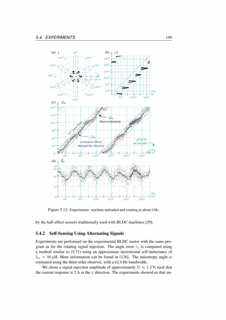
5.4. EXPERIMENTS 199
(b)(a)
(c)
(d)
240
10 15 20 A
60
330
300
270
210
180
150
120
90
30
α
30
90
150
210
270
330
ϕq
90 210 330
33027021015090300
30
60
90
120
150
180
ϕq
33027021015090300
30
20
10
ϕq
µH
15 err
orlin
es
∠ii
·ϕx
·ϕx
direct estimation
/ϕx
estimation filtredthrough the observer
an encodergiven by
·lt-
Figure 5.12: Experiments: machine unloaded and rotating at about 6 Hz.
by the hall-effect sensors traditionally used with BLDC machines [29].
5.4.2 Self-Sensing Using Alternating Signals
Experiments are performed on the experimental BLDC motor with the same pro-gram as for the rotating signal injection. The angle error εx is computed usinga method similar to (5.71) using an approximate incremental self-inductance oflt+ = 80µH. More information can be found in [126]. The anisotropy angle isestimated using the third order observer, with a 62.6 Hz bandwidth.
We chose a signal-injection amplitude of approximately Vi ≈ 1.2 V, such thatthe current response is 2 A in the y direction. The experiments showed us that un-
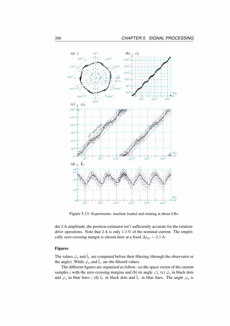
200 CHAPTER 5. SIGNAL PROCESSING
(b)(a)
(c)
(d)
240
10 15 20 A
60
330
300
270
210
180
150
120
90
30
α
30
90
150
210
270
330
ϕq
90 210 330
33027021015090300
30
60
90
120
150
180
ϕq
33027021015090300
30
20
10
ϕq
µH
∠ii
15 err
orlin
es
·lt-
·ϕx
Figure 5.13: Experiments: machine loaded and rotating at about 6 Hz.
der 2 A amplitude, the position estimator isn’t sufficiently accurate for the rotation-drive operations. Note that 2 A is only 1.5 % of the nominal current. The empiri-cally zero-crossing margin is chosen here at a fixed ∆im = 2.1 A.
Figures
The values ϕx and lt- are computed before their filtering (through the observator orthe angle). While ϕx and lt- are the filtered values.
The different figures are organized as follow: (a) the space vector of the currentsamples i with the zero-crossing margins and (b) its angle ∠i; (c) ϕx in black dotsand ϕx in blue lines ; (d) lt- in black dots and lt- in blue lines. The angle ϕq is

5.4. EXPERIMENTS 201
(b)(a)
(c)
(d)
240
10 15 20 A
60
330
300
270
210
180
150
120
90
30
α
30
90
150
210
270
330
ϕq
90 210 330
33027021015090300
30
60
90
120
150
180
ϕq
33027021015090300
30
20
10
ϕq
µH
30 err
orlin
es
∠ii
·ϕx
·lt-
Figure 5.14: Experiments: machine unloaded and rotating at about 60 Hz.
measured by an encoder (not used in the control scheme).
Results
These results were published in [126].The two first experimental results shown in Figure 5.12 and Figure 5.13 are
performed with a low rotating machine around 6 Hz (5 % of the nominal speed).The two next shown Figure 5.14 and Figure 5.15 are performed with a machinerotating around 60 Hz (51 % of the nominal speed). The load corresponds to acurrent stator current of about 15 A amplitude (11 % of the nominal current). Thedistortion on ϕx with respect to ϕd and the variations of lt- are due to the harmonic

202 CHAPTER 5. SIGNAL PROCESSING
(b)(a)
(c)
(d)
240
10 15 20 A
60
330
300
270
210
180
150
120
90
30
α
30
90
150
210
270
330
ϕq
90 210 330
33027021015090300
30
60
90
120
150
180
ϕq
33027021015090300
30
20
10
ϕq
µH
15 err
orlin
es
∠ii
·lt-
·ϕx
Figure 5.15: Experiments: machine loaded and rotating at about 60 Hz.
content in the anisotropy. No correction for the influence of this harmonic contenton the estimated position is performed here. The distortions are only smoothed onϕx and lt- due to the observer filtering (bandwidth of 63 Hz).
The position estimation is satisfying at low speed, at no load as well as witha small load. At higher speed however, the current ripples are much larger thanthe margin size and the zero-crossings can not be avoided. This may explain thelarge dispersion of the estimations ϕx (dots). Nevertheless, the observer seems tofilter these distortions since the filtered position ϕx (lines) is still reliable for theself-sensing control. It seems that a small load reduces the shift on the positionestimation at higher speed, probably due to the fact that the current is farther from

5.5. SUMMARY 203
the zero-crossing lines.The oscillating behaviour of the current, specially in Figure 5.15, is far from a
circle. This can be explained by the zero-crossing impact, since a similar behaviouris observed using the traditional BLDC-machine control with position sensors.
5.5 Summary
In this chapter, we firstly introduced the principle of the field-oriented control andwe tried to categorize the numerous different self-sensing methods as follows:
• Back-EMF or Anisotropy-based methods ;
• Using terminal value measurements or extra dedicated sensors ;
• Anisotropy-based methods using the high-frequency signals of the rotation-drive operations, the high-frequency content of the PWM or methods usingadditional high-frequency injection ;
• Using permanent signal-injections or intermittent signal-injections ;
Solutions to the initial polar ambiguity, position error due to significant stator cur-rents and estimation oscillations due to harmonics are addressed.
The next part focuses on the high-frequency signal injection. The discrete-timemodel of the transmittance to be identified is developed. The principle and theassumption required in order to separate the high-frequency operations of the self-sensing from the the low-frequency operations of the rotation-drive are detailed.The solution of the moving average for the filtering implementation is proposedand discussed. Among the types of signal-injections, we developed the operationsof position estimations for the case of:
1. The rotating signal injection ;
2. The pulsating signal injection ;
3. And the so-called alternating signal injection.
The issue of the noise is quickly assessed. The issues regarding the frequencyseparation, the back-EMF impact, the resistance impact on the position estimation,the PWM-VSI nonlinearities, the settling time and the computation requirementsare addressed for the case of rotating signal injection. The conclusions can beextended to the pulsating signal injection. It is shown that higher the frequency,better the operations regarding all these aspects. The optimal frequency is thereforethird of the sampling frequency for rotating signals and half the sampling frequencyfor pulsating signals.
Experiments confirmed the considerations about the frequency and illustratethe high reliability of the high-frequency signal injection methods. It seems thatrotating signal injections offer better accuracy than the pulsating signal injections,

204 CHAPTER 5. SIGNAL PROCESSING
but the experimental conditions were however not comparable. Further experi-ments would be require to compare them rigorously. A first comparison was pro-posed by [54], but it would require further analysis.

Chapter 6
Conclusions and Future Works
This chapter summaries the main results and conclusions obtained in this thesisabout self-sensing control, mentioning the contributions of our research work. Itfinishes by listing the large number of possible topics that could be addressed incontinuation of that work.
6.1 Summary and Contributions
In the last chapter 5, we introduced how important was the knowledge of the rotorposition regarding optimal field-oriented control operations for permanent-magnetmachines. Firstly, an optimal torque production for a certain current amplitude isobtained by orienting the space vector of the current with respect to the permanent-magnets position. In first approximation, this orientation is found in quadratureregarding the axis of the permanents magnets. Secondly, the rotor position and therotating speed are required in position and speed control operations.
As explained in chapter 1, the dedicated sensors used to obtain the position andthe speed present many drawbacks. Instead of these sensors, it is possible to usesome phenomena in the machine it-self containing rotor position information. Theposition can therefore be extracted by on-line estimations of values modelling thesephenomena, using only the phase current measurements and the DC-bus measure-ments. Other solutions using additional dedicated current/voltage sensors, addi-tional samples or modifying the pulse-width modulated signal sent to the voltage-source inverter can be very efficient, but they present a relatively larger complexityand they are therefore not deeply addressed in this work. Among the phenom-ena, the back-EMF yields a simple and confident source of position information,except at low speeds and at standstill. The anisotropy, characterized by the vari-ation of the incremental self-inductance as a function of the current space-vectororientation, is another source of position information valid for a wide speed rangedown to standstill. Back-EMF-based methods are already largely addressed in theliterature. Therefore, this thesis work mainly focused on the anisotropy-based self-sensing methods.
205

206 CHAPTER 6. CONCLUSIONS AND FUTURE WORKS
Many publications assume an ideal sinusoidal variation of the anisotropic char-acteristics along the air-gap for their machine models. As introduced in chap-ter 2, if this simplification is valid, the incremental self-inductance should varysynchronously with the rotor position. In our experimental Brushless-DC motorhowever, important high-harmonic contents in the magnetic fields and in the statorconductor distributions create an oscillation of the anisotropy as a function of therotor position. We referred to this as an “anisotropy misalignment”. An approachedanalytical model of the anisotropy highlighting this oscillating misalignment waspublished in [92]. Another misalignment, met in about all the machines, is due tothe contribution of the currents along the quadratic axis. This contribution mod-ifies the saturation levels in the machine in addition to the saturation due to thepermanent-magnets fixed to the rotor. This misalignment is generally modeled asan error shift as a function of the currents. Another analytical model taking thecurrents into account was published in [39]. The chapter 2 of this thesis completedthese models and provided tools to assess different impacts of the harmonics. Forour experimental bench, it was firstly shown that the permanent-magnet contri-bution to the magnetic flux as a function of the rotor position mainly contains afundamental component and only a small 5th rank harmonic. By consequence, thismachine could reasonably be commanded as a synchronous machine, leading toa small oscillating torque related to the small 5th rank harmonic. Note that thisoscillating torque is to be compared to the huge cogging torque due to the inter-action between stator teeth and permanent magnets, that was not modelled. It wassecondly shown that the anisotropic incremental self-inductances contain the 2th
rank harmonic, expected to estimate the rotor position, plus a significant −4th rankharmonic, sometimes referred to as ”second saliency” and leading to the oscillat-ing misalignment. Other harmonics were however negligible. The compensationsolutions of the misalignment were addressed in chapter 5.
Upstream of this, methods to identify the incremental self-inductance and to es-timate its anisotropy orientation are needed. All the identification methods requirean accurate knowledge of the supplied voltage. For cost and reliability reasonshowever, the voltage is often not directly measured. In that case, self-sensing op-erations rely on the command voltage sent to the VSI. The behavior of the VSIis however not perfectly linear. In particular, the relation between the expectedoutput voltage and the command voltage is strongly nonlinear when one phasecurrent crosses zero. This is due to a phenomenon known as “zero-clamping” ef-fect. Moreover, the current ripples due to the pulse-width modulation techniqueused to command most of the VSI are generally not measured and they compli-cate any attempt to compensate for the zero-clamping effect. This effect is verysignificant in our experimental bench because of the relatively low inductance ofthe machine, leading to large ripples and frequent zero-crossings. A first solutionpreventing zero-crossings, and thus reducing the zero-clamping impact, was pub-lished in [125]. Improvements were made and implemented in [126] and [163].They are detailed in chapter 4. These solutions were absolutely required in theframe of our experiments, but they inevitably affect the performances of the con-

6.1. SUMMARY AND CONTRIBUTIONS 207
trol. For further researches, it is therefore advised to use other technologies andmachine characteristics that do not present these problems.
We mainly focussed on self-sensing operations using signal injection at dif-ferent high-frequencies, using current samples and based on discrete-time opera-tions. A discrete-time model of the machine was therefore advised. In most ofthe publications, it is assumed that the discrete-time model can be represented asa first-order hold of the continuous-time model during the sampling periods. Butexperimentally, we observed unexpected variations of the model parameter valuesas a function of the injected signal frequency and as a function of the samplingfrequency. The good understanding of these variations were required in order toeliminate any possible error in the implementation or to possibly discover any un-modelled phenomenon. A long development taking discretization effects and tak-ing the pulse-width modulation into account was addressed in chapter 4, neglectingthe eddy currents and taking the eddy currents into account. Comparing the theorywith the experimental results at standstill, it was observed that the eddy currentshave a significant impact on the apparent values of the discrete-time model of ourexperimental machine. These variations were however not dramatic for the perfor-mances of the self-sensing operations.
Many different types of high-frequency signals can be injected in the machinein order to identify the incremental self-inductance. They are overview and com-pared in chapter 5. Adaptive test signals were used in [169], permanent pulsatingsignals at half the sampling frequency were analyzed in [126] and permanent rotat-ing signals up to one-third the sampling frequency were studied in [163]. In manyaspects, the use of the maximum frequency in signal injection present importantbenefits. The first one is related to the error in the anisotropy estimation due tothe presence of a resistance in the model for rotating signals (the pulsating sig-nals do not experience that problem). Most of the self-sensing methods based onhigh-frequency signal-injections assume that the electrical-circuit of the machinebehaves as a purely integrator (inductive behaviour): the variations of the currentsare assumed directly proportional to the injected voltages, where the proportionalfactor is the incremental self-inductance. This assumption is however not validin the experimental Brushless-DC motor due to significant resistive voltage drops,mainly due to eddy currents. Even if the eddy current contribution tends to in-crease with the frequency to some extent, as explained in chapter 4, it was howevershown that their impacts on the self-sensing operations tend to decrease with thefrequency of the injected signal. Other analyzed aspects are the separation betweenthe self-sensing and the rotation-drive operations. This is of upmost importance inorder to prevent mutual interactions and, possibly, to reduce the efficiency of thecontrol. This separation is generally done by filtering operations. The quality ofthe filtering however depends on the gap between the frequencies used for bothoperations. Higher the injected-signal frequency, better is this gap. The optimaladvised frequency is therefore the highest one. These conclusions concern the per-manent signals. The test signals are equivalent to intermittent pulsating signals.Further issues concerning the remaining impact of the test signals on the control

208 CHAPTER 6. CONCLUSIONS AND FUTURE WORKS
operations, mainly due to the resistance, were addressed in [169].The main conclusion concerning the experimental bench was that the use of
such a Brushless-DC motor is not really advised in real applications requiring self-sensing, due to all the problems concerning the harmonics and the zero-clampingeffects. It was however very interesting to implement self-sensing methods on thatbench for scientific purposes in order to highlight all these undesired effects and toassess their impacts, since they exist anyway in all machines in a lesser extent andthey could be considered to improve the control. For example, it allowed to demon-strate the robustness of the signal-injection techniques at the highest frequencies.It would now be recommendable to perform further analysis on other machines,with better characteristics, in order to assess the reachable accuracy.
6.2 Future Works
The final implementation of the self-sensing methods were very satisfying, but stillincomplete to be transposed in industrial applications without further considera-tions and validations. Much work remains, but the numerous theoretical modelsand tools, plus the different proposed methods prepared the ground to future worksand opens up the possibility of success in a short time. We suggest hereafter sometopics for future works in the frame of this thesis:
• The impact of the load current on the anisotropy ratio and on the anisotropymisalignment have been theoretically analyzed. The theoretical model per-mitted to perform some observations on the experimental BLDC motor upto a reduced torque and a reduced speed. These limitations were inheritedfrom hardware and power source capacities of the test bench. Experimentson the full ranges up to the rated values still remain to be performed in or-der to draw maps of feasibility regions. This could probably leads to newobservations and conclusions about the experimental motor ;
• Some publications already drew maps of feasibility regions for anisotropy-based self-sensing operations as a function of the load current [66, 62, 63,58, 59, 55, 65, 67, 60, 61, 64]. They are even computed using finite-elementsimulations, treating with variation of some small elements in order to high-light some benefits. Or they are proposing comparisons of different machinedesigns. This comparative methodology however takes much time and, byconsequence, a lot of work remains with the many different possible ma-chine designs. In order to accelerate this research, simple analytical modelsof the load impact, represented by the angular factor m(θ), could eventuallybe developped and coupled to the model of the incremental self-inductanceproposed in the first chapter. We see some opportunities offered by thatmethodology in the selection of optimal designs. This is an open topic ;
• As explained in the last chapter, some authors already proposed angular cor-rections of the anisotropy misalignment as a function of the load current and

6.2. FUTURE WORKS 209
of the secondary anisotropy [53, 56, 158]. None of these methods, or anyother method, were implemented and experimented in this work due to lackof time. This could however strongly increase the accuracy and improve thecontrol, reducing the oscillations on the position estimation. A promisingsolution combines the back-EMF-based and the anisotropy-base self-sensing[57, 115, 167, 177]. Each of these source of position information could beused in order to mutually compensated for their errors. This is a signifi-cant evolution compared to hybrid solutions simply commutating betweenone to the other source of position over a speed threshold, as proposed in[133, 143, 114] ;
• The inverter nonlinearities were very annoying in this study. Due to the ad-ditional torque ripples and the computation complexity, the solution of zero-crossing prevention that we proposed could be discouraging for the industryand we have no great hope for the future of this solution. Other types ofvoltage source or other topologies, for instance using the neutral connectionpoint, could possibly remove part of these problems and strongly improvethe position estimation at higher speeds. This topic is however lying in fal-low ;
• Between the different types of high-frequency signals were used in this work.Results suggested that rotating signal-injections presented better accuracythan pulsating signal-injection. Further experiments in comparable condi-tions should be performed in order to quantitatively assess this issue. Itwould also be interesting to further compare these permanent signal injec-tions with intermittent signals injections, such as the test pulses proposed by[154]. This could probably be performed without much effort ;
• We mainly focused on the high-frequency injection using the controller sen-sors. Even if the use of extra dedicated sensors present some important draw-backs, it could however be interesting to compare their accuracy with thesolution using controller sensors under similar conditions, since they couldbe more interesting for applications where the quality of the control is moreimportant than the cost and the robustness ;
• Finally, the signal-injection method could be extended to multiphase ma-chines (i.e. more than 3-phases). The theory presented in chapter 5 isindependent to the number of phases and applications to multiphase ma-chines were already published [188]. Possible interactions of the fundamen-tal space-vectors, i.e. x(1) with other harmonic orders in the machine, as de-scribed in chapter 2, should however be analyzed. The multiphase machinesalso present important benefits with respect to the fault-tolerance capacity,by maintaining drives under a smaller number of phases, even with reducedperformances. Application to faulty three-phase machines was proposed by

210 CHAPTER 6. CONCLUSIONS AND FUTURE WORKS
[189]. But the case self-sensing methods applied to faulty multiphase ma-chines could be a excellent topic of research.
Bibliography
[1] I. Boldea, “Control issues in adjustable speed drives,” IEEE Industrial Elec-tronics Magazine, vol. 2, pp. 32 – 50, Sept. 2008.
[2] J. Finch and D. Giaouris, “Controlled ac electrical drives,” IEEE Transac-tions on Industrial Electronics, vol. 55, pp. 481 – 491, Feb. 2008.
[3] C. Espanet, J.-M. Kauffmann, and R. Bernard, “Comparison of two in-wheelpermanent magnet motors for military applications,” in IEEE Vehicle Powerand Propulsion Conference (VPPC), pp. 1 – 6, Sept. 2006.
[4] G. Khalil, “Challenges of hybrid electric vehicles for military applications,”in IEEE Vehicle Power and Propulsion Conference (VPPC), pp. 1 – 3, Sept.2009.
[5] J. Holtz, “Sensorless control of induction machines - with or without signalinjection ?,” IEEE Transactions on Industrial Electronics, vol. 53, pp. 7 –30, Feb. 2005.
[6] P. Acarnley and J. Watson, “Review of position-sensorless operation ofbrushless permanent-magnet machines,” IEEE Transactions on IndustrialElectronics, vol. 53, pp. 352 – 362, Apr. 2006.
[7] M. Pacas, “Sensorless drives in industrial applications,” IEEE IndustrialElectronics Magazine, vol. 5, pp. 16 – 23, June 2011.
[8] E. Vazquez-Sanchez, J. Gomez-Gil, J. Gamazo-Real, and J. Diez-Higuera,“A new method for sensorless estimation of the speed and position inbrushed dc motors using support vector machines,” IEEE Transactions onIndustrial Electronics, vol. 59, pp. 1397 – 1408, Mar. 2012.
[9] L. Xu, E. Inoa, Y. Liu, and B. Guan, “A new high-frequency injectionmethod for sensorless control of doubly fed induction machines,” IEEETransactions on Industry Applications, vol. 48, pp. 1556 – 1564, Sept. 2012.
[10] P. Vas, Electrical Machines and Drives: A Space-Vector Theory Approach.United States: Oxford University Press, 1993.
211

212 BIBLIOGRAPHY
[11] J.-P. Caron and J.-P. Hautier, Modelisation et commande de la machine asyn-chrome. Methodes et pratiques de l’ingenieur, 75737 Paris, France: Technip,1995.
[12] G. Sturtzer and E. Smigiel, Modelisation et commande des moteurstriphases. Technosup, 75740 Paris, France: Ellipses Marketing, 2000.
[13] M. Correvon, Electronique de puissance. France: Haute Ecole d’Ingenierieet de Gestion du Canton du Vaud, 2006.
[14] R. H. Park, “Two-reaction theory of synchronous machines: Generalizedmethod of analysis - part i,” American Institute of Electrical Engineers(AIEE), pp. 716 – 727, July 1929.
[15] R. H. Park, “Two-reaction theory of synchronous machines-ii,” Transactionsof the American Institute of Electrical Engineers, vol. 52, pp. 352 – 354,June 1933.
[16] I. H. Summers, “Vector theory of circuits involving synchronous machines,”Transactions of the American Institute of Electrical Engineers, vol. 51,pp. 318 – 321, June 1932.
[17] S. B. Crary, “Two-reaction theory of synchronous machines,” Transactionsof the American Institute of Electrical Engineers, vol. 56, pp. 27 – 36, Jan.1937.
[18] J. Holtz, “Pulsewidth modulation for electronic power conversion,” Pro-ceedings of the IEEE, vol. 82, pp. 1194 – 1214, Aug. 1994.
[19] G. Maggetto, Contribution A l’Etude Du Comportement Des Moteurs Asyn-chrones Alimentes Par Convertisseurs Statiques. PhD thesis, Universite Li-bre de Bruxelles, 1973.
[20] H. Fudeh and C. Ong, “Modeling and analysis of induction machines cona-tining space harmonics part i: Modeling and transformation,” IEEE Trans-actions on Power Apparatus and Systems, vol. PAS-102, pp. 2608 – 2615,Aug. 1983.
[21] H. Fudeh and C. Ong, “Modeling and analysis of induction machines cona-tining space harmonics part ii: Analysis of asynchronous and synchronousactions,” IEEE Transactions on Power Apparatus and Systems, vol. PAS-102, pp. 2616 – 2620, Aug. 1983.
[22] H. Fudeh and C. Ong, “Modeling and analysis of induction machinesconatining space harmonics part iii: Three-phase cage rotor induction ma-chines,” IEEE Transactions on Power Apparatus and Systems, vol. PAS-102,pp. 2621 – 2628, Aug. 1983.

BIBLIOGRAPHY 213
[23] F. D. Belie, J. Melkebeek, K. Geldhof, L. Vandevelde, and R. Boel,“A general description of high-frequency position estimators for interiorpermanent-magnet synchronous motors,” in International Conference onElectrical Machines (ICEM), Sept. 2004.
[24] J. Faiz and I. Tabatabaei, “Extension of winding function theory for nonuni-form air gap in electric machinery,” IEEE Transactions on Magnetics,vol. 38, pp. 3654 – 3657, Nov. 2002.
[25] H. Toda, Z. Xia, J. Wang, K. Atallah, and D. Howe, “Rotor eddy-currentloss in permanent magnet brushless machines,” IEEE Transactions on Mag-netics, vol. 40, pp. 2104 – 2106, July 2004.
[26] L. James and J. Kirtley, 6.685 Electric Machines. Massachusetts - USA: De-partment of Electrical Engineering and Computer Science - MassachusettsInstitute of Technology, 2005.
[27] J. Gyselinck, ELEC269 Genie electrique. Brussels - Belgium: DepartementBeams - Universite Libre de Bruxelles, 2006.
[28] J.-P. Vilain, A. Vauquelin, S. Vivier, and B. D. Nicolas Labbe, “Behavioranalysis of a dc brush machine by space vector theory,” in InternationalConference on Electrical Machines (ICEM), Sept. 2010.
[29] T. Jahns and W. Soong, “Pulsating torque minimization techniques for per-manent magnet ac motor drives-a review,” IEEE Transactions on IndustrialElectronics, vol. 43, pp. 321 – 330, Apr. 1996.
[30] J. Melkebeek, “Small signal dynamic modelling of saturated synchronousmachines,” in International Conference on Electrical Machines (ICEM),no. 2, pp. 447 – 450, Sept. 1984.
[31] F. De Belie, J. Melkebeek, L. Vandevelde, R. Boel, K. Geldhof, andT. Vyncke, “A nonlinear model for synchronous machines to describe high-frequency signal based position estimators,” in IEEE International Confer-ence on Electric Machines and Drives, pp. 696 – 703, May 2005.
[32] M.-J. Chung and D.-G. Gweon, “Modeling of the armature slotting effect inthe magnetic field distribution of a linear permanent magnet motor,” Elec-trical Engineering (Archiv fur Elektrotechnik), vol. 84, pp. 101–108, 2002.10.1007/s00202-001-0108-0.
[33] T. Lubin, S. Mezani, and A. Rezzoug, “2-d exact analytical model forsurface-mounted permanent-magnet motors with semi-closed slots,” IEEETransactions on Magnetics, vol. 47, pp. 479 – 492, Feb. 2011.
[34] Z. Zhu and D. Howe, “Instantaneous magnetic field distribution in brushlesspermanent magnet dc motors. ii. armature-reaction field,” IEEE Transac-tions on Magnetics, vol. 29, pp. 136 – 142, Jan. 1993.

214 BIBLIOGRAPHY
[35] Z. Zhu, D. Howe, E. Bolte, and B. Ackermann, “Instantaneous magneticfield distribution in brushless permanent magnet dc motors. i. open-circuitfield,” IEEE Transactions on Magnetics, vol. 29, pp. 124 – 135, Jan. 1993.
[36] J. Chiasson, Modeling and high performance control of electric machines.USA: IEEE Computer Society Press, 2005.
[37] I. A. Viorel and L. Hamemeyer, K. ; Strete, “On the carter’s factor calcu-lation for slotted electric machines,” Advances in Electrical and ComputerEngineering, vol. 7, no. 2, pp. 55 – 58, 2007.
[38] K. Boughrara, R. Ibtiouen, D. Z andarko, O. Touhami, and A. Rez-zoug, “Magnetic field analysis of external rotor permanent-magnet syn-chronous motors using conformal mapping,” IEEE Transactions on Mag-netics, vol. 46, pp. 3684 – 3693, Sept. 2010.
[39] F. Gabriel, F. De Belie, P. Sergeant, and X. Neyt, “Modelling the impactof the stator currents on inductance-based sensorless control of brushlessdc-machines,” in Symposium on Sensorless Control for Electrical Drives(SLED), pp. 56 – 63, IEEE, Sept. 2011.
[40] J.-I. Ha, “Analysis of inherent magnetic position sensors in symmetric acmachines for zero or low speed sensorless drives,” IEEE Transactions onMagnetics, vol. 44, pp. 4689 – 4696, Dec. 2008.
[41] S.-C. Yang, T. Suzuki, R. Lorenz, and T. Jahns, “Surface-permanent-magnetsynchronous machine design for saliency-tracking self-sensing position es-timation at zero and low speeds,” IEEE Transactions on Industry Applica-tions, vol. 47, pp. 2103 – 2116, Sept. 2011.
[42] Z. Zhu and D. Howe, “Instantaneous magnetic field distribution in brushlesspermanent magnet dc motors. iii. effect of stator slotting,” IEEE Transac-tions on Magnetics, vol. 29, pp. 143 –151, Jan. 1993.
[43] Y. Kano, T. Kosaka, and N. Matsui, “Simple nonlinear magnetic analysis forpermanent-magnet motors,” IEEE Transactions on Industry Applications,vol. 41, pp. 1205 – 1214, Sept. 2005.
[44] B. Cassimere, S. Sudhoff, and D. Sudhoff, “Analytical design model forsurface-mounted permanent-magnet synchronous machines,” IEEE Trans-actions on Energy Conversion, vol. 24, pp. 347 – 357, June 2009.
[45] L. Schreier, J. Bendl, M. Chomat, and M. Skalka, “Influence of space har-monics on properties of six-phase induction machine - part i. analysis,” inInternational Conference on Electrical Machines (ICEM), Sept. 2010.
[46] A. V. Oppenheim and R. W. Schafer, Digital signal processing. Prentice-Hall, 1975.
BIBLIOGRAPHY 215
[47] W. Wang, K. Nam, and S. young Kim, “Concentric winding bldc motordesign,” in IEEE International Conference on Electric Machines and Drives,pp. 157 – 161, May 2005.
[48] Y. Wu, Z. Deng, X. Wang, X. Ling, and X. Cao, “Position sensorless controlbased on coordinate transformation for brushless dc motor drives,” IEEETransactions on Power Electronics, vol. 25, pp. 2365 – 2371, Sept. 2010.
[49] J. Moreira and T. Lipo, “Modeling of saturated ac machines including airgap flux harmonic components,” IEEE Transactions on Industry Applica-tions, vol. 28, pp. 343 – 349, Mar. 1992.
[50] H.-W. Lee, T.-H. Kim, and M. Ehsani, “Power density maximization of thebrushless dc generator,” in IEEE Annual Conference of Industrial Electron-ics Society (IECON), vol. 3, pp. 2162 – 2166, Nov. 2003.
[51] F. Meinguet, E. Semail, and J. Gyselinck, “Enhanced control of a pmsm sup-plied by a four-leg voltage source inverter using the homopolar torque,” inProceedings of the XVIII International Conference on Electrical Machines(IEMDC), 2008.
[52] P. Landsmann, D. Paulus, P. Stolze, and R. Kennel, “Saliency based en-coderless predictive torque control without signal injection for a reluctancesynchronous machine,” in International Power Electronics and Motion Con-trol Conference (EPE/PEMC), pp. S1–10 – S1–17, Sept. 2010.
[53] M. Degner and R. Lorenz, “Using multiple saliencies for the estimation offlux, position, and velocity in ac machines,” IEEE Transactions on IndustryApplications, vol. 34, pp. 1097 – 1104, Sept. 1998.
[54] D. Raca, P. Garcia, D. Reigosa, F. Briz, and R. Lorenz, “A comparative anal-ysis of pulsating vs. rotating vector carrier signal injection-based sensorlesscontrol,” in Applied Power Electronics Conference and Exposition (APEC),pp. 879 – 885, Feb. 2008.
[55] S. Wu, D. Reigosa, Y. Shibukawa, M. Leetmaa, R. Lorenz, and Y. Li,“Interior permanent-magnet synchronous motor design for improving self-sensing performance at very low speed,” IEEE Transactions on Industry Ap-plications, vol. 45, pp. 1939 – 1946, Nov. 2009.
[56] E. Kayikci and R. Lorenz, “Self-sensing methods extended to four phaseswitched reluctance machines,” in Power Electronics Conference (IPEC),pp. 2016 – 2023, June 2010.
[57] I. Boldea, M. Paicu, and G.-D. Andreescu, “Active flux concept for motion-sensorless unified ac drives,” IEEE Transactions on Power Electronics,vol. 23, pp. 2612 –2618, Sept. 2008.
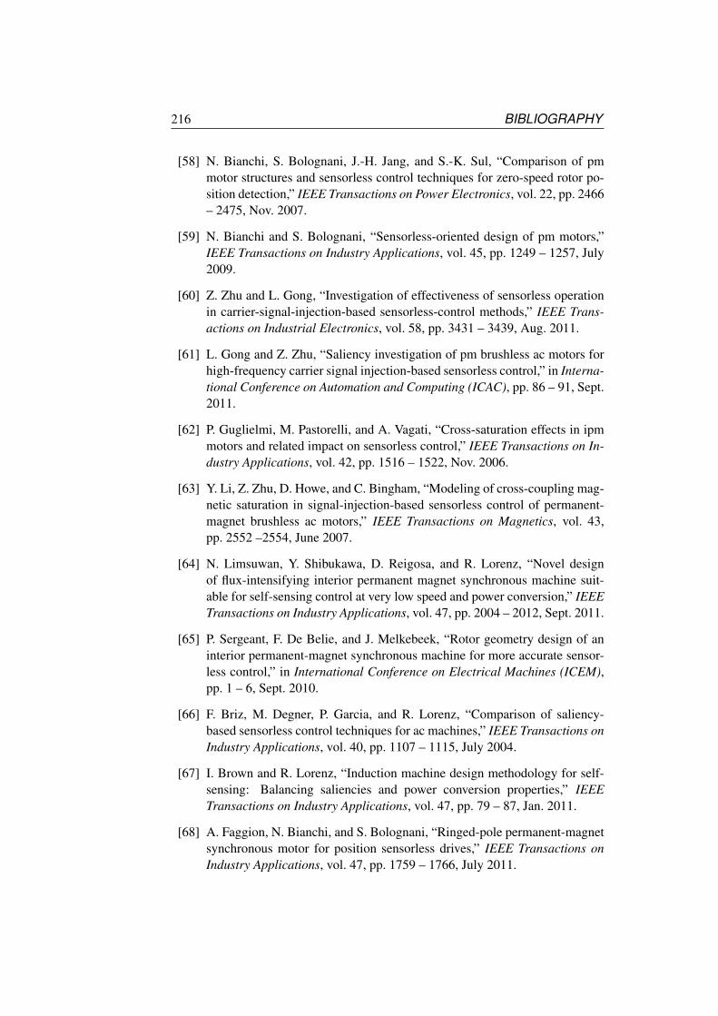
216 BIBLIOGRAPHY
[58] N. Bianchi, S. Bolognani, J.-H. Jang, and S.-K. Sul, “Comparison of pmmotor structures and sensorless control techniques for zero-speed rotor po-sition detection,” IEEE Transactions on Power Electronics, vol. 22, pp. 2466– 2475, Nov. 2007.
[59] N. Bianchi and S. Bolognani, “Sensorless-oriented design of pm motors,”IEEE Transactions on Industry Applications, vol. 45, pp. 1249 – 1257, July2009.
[60] Z. Zhu and L. Gong, “Investigation of effectiveness of sensorless operationin carrier-signal-injection-based sensorless-control methods,” IEEE Trans-actions on Industrial Electronics, vol. 58, pp. 3431 – 3439, Aug. 2011.
[61] L. Gong and Z. Zhu, “Saliency investigation of pm brushless ac motors forhigh-frequency carrier signal injection-based sensorless control,” in Interna-tional Conference on Automation and Computing (ICAC), pp. 86 – 91, Sept.2011.
[62] P. Guglielmi, M. Pastorelli, and A. Vagati, “Cross-saturation effects in ipmmotors and related impact on sensorless control,” IEEE Transactions on In-dustry Applications, vol. 42, pp. 1516 – 1522, Nov. 2006.
[63] Y. Li, Z. Zhu, D. Howe, and C. Bingham, “Modeling of cross-coupling mag-netic saturation in signal-injection-based sensorless control of permanent-magnet brushless ac motors,” IEEE Transactions on Magnetics, vol. 43,pp. 2552 –2554, June 2007.
[64] N. Limsuwan, Y. Shibukawa, D. Reigosa, and R. Lorenz, “Novel designof flux-intensifying interior permanent magnet synchronous machine suit-able for self-sensing control at very low speed and power conversion,” IEEETransactions on Industry Applications, vol. 47, pp. 2004 – 2012, Sept. 2011.
[65] P. Sergeant, F. De Belie, and J. Melkebeek, “Rotor geometry design of aninterior permanent-magnet synchronous machine for more accurate sensor-less control,” in International Conference on Electrical Machines (ICEM),pp. 1 – 6, Sept. 2010.
[66] F. Briz, M. Degner, P. Garcia, and R. Lorenz, “Comparison of saliency-based sensorless control techniques for ac machines,” IEEE Transactions onIndustry Applications, vol. 40, pp. 1107 – 1115, July 2004.
[67] I. Brown and R. Lorenz, “Induction machine design methodology for self-sensing: Balancing saliencies and power conversion properties,” IEEETransactions on Industry Applications, vol. 47, pp. 79 – 87, Jan. 2011.
[68] A. Faggion, N. Bianchi, and S. Bolognani, “Ringed-pole permanent-magnetsynchronous motor for position sensorless drives,” IEEE Transactions onIndustry Applications, vol. 47, pp. 1759 – 1766, July 2011.

BIBLIOGRAPHY 217
[69] M. Morandin, S. Bolognani, and A. Faggion, “Outer-rotor ringed-pole spmstarter-alternator suited for sensorless drives,” in Symposium on SensorlessControl for Electrical Drives (SLED), pp. 96 – 101, Sept. 2011.
[70] H. Mai, F. Dubas, D. Chamagne, and C. Espanet, “Optimal design of a sur-face mounted permanent magnet in-wheel motor for an urban hybrid vehi-cle,” in Vehicle Power and Propulsion Conference (VPPC), pp. 481 – 485,Sept. 2009.
[71] Z. Zhu and D. Howe, “Instantaneous magnetic field distribution in perma-nent magnet brushless dc motors. iv. magnetic field on load,” IEEE Trans-actions on Magnetics, vol. 29, pp. 152 – 158, Jan. 1993.
[72] V. Donescu, A. Charette, Z. Yao, and V. Rajagopalan, “Modeling and simu-lation of saturated induction motors in phase quantities,” IEEE Transactionson Energy Conversion, vol. 14, pp. 386 – 393, Sept. 1999.
[73] H. Kim, M. Degner, J. Guerrero, F. Briz, and R. Lorenz, “Discrete-time cur-rent regulator design for ac machine drives,” IEEE Transactions on IndustryApplications, vol. 46, pp. 1425 – 1435, July 2010.
[74] A. Navarrete, J. Rivera, J. Raygoza, and S. Ortega, “Discrete-time modelingand control of pmsm,” in Electronics, Robotics and Automotive MechanicsConference (CERMA), pp. 258 – 263, Nov. 2011.
[75] A. Loukianov, A. Navarrete, J. Rivera, and S. Ortega-Cisneros, “Discrete-time sensorless control of permanent magnet synchronous motors,” in Con-ference on Electrical Engineering Computing Science and Automatic Con-trol (CCE), pp. 1 – 6, Oct. 2011.
[76] I. Boldea and S. Nasar, “A general equivalent circuit (gec) of electric ma-chines including cross-coupling saturation and frequency effects,” IEEETransactions on Energy Conversion, vol. 3, pp. 689 – 695, Sept. 1988.
[77] D. Raca, P. Garcia, D. Reigosa, F. Briz, and R. Lorenz, “Carrier-signal se-lection for sensorless control of pm synchronous machines at zero and verylow speeds,” IEEE Transactions on Industry Applications, vol. 46, pp. 167– 178, Jan. 2010.
[78] B. Stumberger, G. Stumberger, D. Dolinar, A. Hamler, and M. Trlep, “Eval-uation of saturation and cross-magnetization effects in interior permanent-magnet synchronous motor,” IEEE Transactions on Industry Applications,vol. 39, pp. 1264 – 1271, Sept. 2003.
[79] S. Ostlund and M. Brokemper, “Sensorless rotor-position detection fromzero to rated speed for an integrated pm synchronous motor drive,” IEEETransactions on Industry Applications, vol. 32, pp. 1158 – 1165, Sept. 1996.

218 BIBLIOGRAPHY
[80] W. Roshen, “Iron loss model for permanent-magnet synchronous motors,”IEEE Transactions on Magnetics, vol. 43, pp. 3428 – 3434, Aug. 2007.
[81] J. Wang, K. Atallah, R. Chin, W. Arshad, and H. Lendenmann, “Rotor eddy-current loss in permanent-magnet brushless ac machines,” IEEE Transac-tions on Magnetics, vol. 46, pp. 2701 – 2707, July 2010.
[82] S.-C. Yang and R. Lorenz, “Analysis of iron and magnet losses in surfacepermanent magnet machines resulting from injection-based self-sensing po-sition estimation,” in Energy Conversion Congress and Exposition (ECCE),pp. 630 – 637, Sept. 2011.
[83] S. Moulahoum and O. Touhami, “A saturated induction machine model withseries iron losses resistance,” in International Conference on Power Engi-neering, Energy and Electrical Drives, pp. 156 – 161, Apr. 2007.
[84] S. Bolognani, L. Peretti, M. Zigliotto, and E. Bertotto, “Commissioning ofelectromechanical conversion models for high dynamic pmsm drives,” IEEETransactions on Industrial Electronics, vol. 57, pp. 986 – 993, Mar. 2010.
[85] S.-C. Yang and R. Lorenz, “Surface permanent magnet synchronous ma-chine position estimation at low speed using eddy-current-reflected asym-metric resistance,” IEEE Transactions on Power Electronics, vol. 27,pp. 2595 – 2604, May 2012.
[86] M. R. Spiegel, Formules et tables de mathematiques. Serie Schaum, 75014Paris, France: Mac Graw Hill, 1992.
[87] J. Holtz, “Pulsewidth modulation-a survey,” IEEE Transactions on Indus-trial Electronics, vol. 39, pp. 410 – 420, Oct. 1992.
[88] N. Urasaki, T. Senjyu, and K. Uezato, “Relationship of parallel model andseries model for permanent magnet synchronous motors taking iron loss intoaccount,” IEEE Transactions on Energy Conversion, vol. 19, pp. 265 – 270,June 2004.
[89] P. Sergeant, F. De Belie, L. Dupre, and J. Melkebeek, “Losses in sensorlesscontrolled permanent-magnet synchronous machines,” IEEE Transactionson Magnetics, vol. 46, pp. 590 – 593, Feb. 2010.
[90] D. Reigosa, P. Garcia, F. Briz, D. Raca, and R. Lorenz, “Modeling andadaptive decoupling of high-frequency resistance and temperature effects incarrier-based sensorless control of pm synchronous machines,” IEEE Trans-actions on Industry Applications, vol. 46, pp. 139 – 149, Jan. 2010.
[91] N. Limsuwan, T. Kato, C.-Y. Yu, J. Tamura, D. Reigosa, K. Akatsu, andR. Lorenz, “Secondary resistive losses with high-frequency injection-basedself-sensing in ipm machines,” in Energy Conversion Congress and Exposi-tion (ECCE), pp. 622 – 629, Sept. 2011.
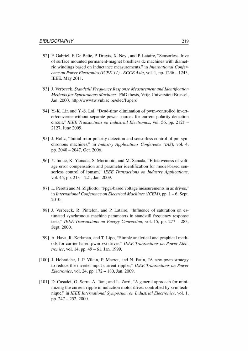
BIBLIOGRAPHY 219
[92] F. Gabriel, F. De Belie, P. Druyts, X. Neyt, and P. Lataire, “Sensorless driveof surface mounted permanent-magnet brushless dc machines with diamet-ric windings based on inductance measurements,” in International Confer-ence on Power Electronics (ICPE’11) - ECCE Asia, vol. 1, pp. 1236 – 1243,IEEE, May 2011.
[93] J. Verbeeck, Standstill Frequency Response Measurement and IdentificationMethods for Synchronous Machines. PhD thesis, Vrije Universiteit Brussel,Jan. 2000. http://wwwtw.vub.ac.be/elec/Papers
[94] Y.-K. Lin and Y.-S. Lai, “Dead-time elimination of pwm-controlled invert-er/converter without separate power sources for current polarity detectioncircuit,” IEEE Transactions on Industrial Electronics, vol. 56, pp. 2121 –2127, June 2009.
[95] J. Holtz, “Initial rotor polarity detection and sensorless control of pm syn-chronous machines,” in Industry Applications Conference (IAS), vol. 4,pp. 2040 – 2047, Oct. 2006.
[96] Y. Inoue, K. Yamada, S. Morimoto, and M. Sanada, “Effectiveness of volt-age error compensation and parameter identification for model-based sen-sorless control of ipmsm,” IEEE Transactions on Industry Applications,vol. 45, pp. 213 – 221, Jan. 2009.
[97] L. Peretti and M. Zigliotto, “Fpga-based voltage measurements in ac drives,”in International Conference on Electrical Machines (ICEM), pp. 1 – 6, Sept.2010.
[98] J. Verbeeck, R. Pintelon, and P. Lataire, “Influence of saturation on es-timated synchronous machine parameters in standstill frequency responsetests,” IEEE Transactions on Energy Conversion, vol. 15, pp. 277 – 283,Sept. 2000.
[99] A. Hava, R. Kerkman, and T. Lipo, “Simple analytical and graphical meth-ods for carrier-based pwm-vsi drives,” IEEE Transactions on Power Elec-tronics, vol. 14, pp. 49 – 61, Jan. 1999.
[100] J. Hobraiche, J.-P. Vilain, P. Macret, and N. Patin, “A new pwm strategyto reduce the inverter input current ripples,” IEEE Transactions on PowerElectronics, vol. 24, pp. 172 – 180, Jan. 2009.
[101] D. Casadei, G. Serra, A. Tani, and L. Zarri, “A general approach for mini-mizing the current ripple in induction motor drives controlled by svm tech-nique,” in IEEE International Symposium on Industrial Electronics, vol. 1,pp. 247 – 252, 2000.

220 BIBLIOGRAPHY
[102] H. Krishnamurthy, G. Narayanan, R. Ayyanar, and V. Ranganathan, “Designof space vector-based hybrid pwm techniques for reduced current ripple,” inIEEE Applied Power Electronics Conference and Exposition, vol. 1, pp. 583– 588, Feb. 2003.
[103] Y. Murai, T. Watanabe, and H. Iwasaki, “Waveform distortion and correctioncircuit for pwm inverters with switching lag-times,” IEEE Transactions onIndustry Applications, vol. 23, pp. 881 – 886, Sept. 1987.
[104] A. Munoz and T. Lipo, “On-line dead-time compensation technique foropen-loop pwm-vsi drives,” IEEE Transactions on Power Electronics,vol. 14, pp. 683 – 689, July 1999.
[105] P. Garcia, F. Briz, M. Degner, and D. Diaz-Reigosa, “Accuracy, bandwidth,and stability limits of carrier-signal-injection-based sensorless control meth-ods,” IEEE Transactions on Industry Applications, vol. 43, pp. 990 – 1000,July 2007.
[106] D. Leggate and R. J. Kerkman, “Pulse-based dead-time compensatorfor pwm voltage inverters,” IEEE Transactions on Industrial Electronics,vol. 44, pp. 191 – 197, Apr. 1997.
[107] T. Summers and R. Betz, “Dead-time issues in predictive current control,”IEEE Transactions on Industry Applications, vol. 40, pp. 835 – 844, May2004.
[108] G. Narayanan, V. Ranganathan, D. Zhao, H. Krishnamurthy, and R. Ayya-nar, “Space vector based hybrid pwm techniques for reduced current ripple,”IEEE Transactions on Industrial Electronics, vol. 55, pp. 1614 – 1627, Apr.2008.
[109] N. Urasaki, T. Senjyu, K. Uezato, and T. Funabashi, “Adaptive dead-timecompensation strategy for permanent magnet synchronous motor drive,”IEEE Transactions on Energy Conversion, vol. 22, pp. 271 – 280, June 2007.
[110] J.-S. Choi, J.-Y. Yoo, S.-W. Lim, and Y.-S. Kim, “A novel dead time mini-mization algorithm of the pwm inverter,” IEEE Industry Applications Con-ference (IAS), vol. 4, pp. 2188 – 2193, 1999.
[111] L. Ben-Brahim, “The analysis and compensation of dead-time effects inthree phase pwm inverters,” Conference of the IEEE Industrial ElectronicsSociety (IECON), vol. 2, pp. 792 – 797, Sept. 1998.
[112] H.-S. Ryu, I.-H. Lim, J.-H. Lee, S.-H. Hwang, and J.-M. Kim, “A dead timecompensation method in voltage-fed pwm inverter,” vol. 2, pp. 911 – 916,Oct. 2006.

BIBLIOGRAPHY 221
[113] J.-W. Choi and S.-K. Sul, “Inverter output voltage synthesis using noveldead time compensation,” IEEE Transactions on Power Electronics, vol. 11,pp. 221 – 227, Mar. 1996.
[114] G. Wang, R. Yang, and D. Xu, “Dsp-based control of sensorless ipmsmdrives for wide-speed-range operation,” IEEE Transactions on IndustrialElectronics, vol. 60, pp. 720 – 727, Feb. 2013.
[115] C. Silva, G. Asher, and M. Sumner, “Hybrid rotor position observer forwide speed-range sensorless pm motor drives including zero speed,” IEEETransactions on Industrial Electronics, vol. 53, pp. 373 – 378, Apr. 2006.
[116] J. Seung-Gi, L. Bang-Sup, K. Kyung-Seo, and P. Min-Ho, “The analysis andcompensation of dead time effects in pwm inverters,” vol. 3, pp. 667 – 671,Oct. 1988.
[117] S.-G. Jeong and M.-H. Park, “The analysis and compensation of dead-time effects in pwm inverters,” IEEE Transactions on Industrial Electronics,vol. 38, pp. 108 – 114, Apr. 1991.
[118] V. Cardenas, S. Horta, and R. Echavarria, “Elimination of dead time effectsin three phase inverters,” pp. 258 – 262, Oct. 1996.
[119] T. Wolbank, M. Vogelsberger, and M. Riepler, “Identification and compen-sation of inverter dead-time effect on zero speed sensorless control of acmachines based on voltage pulse injection,” pp. 2844 – 2849, June 2008.
[120] R. Raute, C. Caruana, C. Staines, J. Cilia, N. Teske, M. Sumner, andG. Asher, “A review of sensorless control in induction machines using hfinjection, test vectors and pwm harmonics,” in Symposium on SensorlessControl for Electrical Drives (SLED), pp. 47 – 55, Sept. 2011.
[121] L. Gong and Z. Zhu, “A novel method for compensating inverter nonlinear-ity effects in carrier signal injection-based sensorless control from positive-sequence carrier current distortion,” IEEE Transactions on Industry Appli-cations, vol. 47, pp. 1283 – 1292, May 2011.
[122] L. Ben-Brahim, “On the compensation of dead time and zero-current cross-ing for a pwm-inverter-controlled ac servo drive,” IEEE Transaction on In-dustrial Electronics, vol. 51, pp. 1113 – 1118, Oct. 2004.
[123] N. Urasaki, T. Senjyu, K. Uezato, and T. Funabashi, “An adaptive dead-timecompensation strategy for voltage source inverter fed motor drives,” IEEETransactions on Power Electronics, vol. 20, pp. 1150 – 1160, Sept. 2005.
[124] C. Silva, G. Asher, and M. Sumner, “Influence of dead-time compensationon rotor position estimation in surface mounted pm machines using hf volt-age injection,” in Power Conversion Conference (PCC), vol. 3, pp. 1279 –1284, 2002.

222 BIBLIOGRAPHY
[125] F. Gabriel, F. De Belie, P. Druyts, and X. Neyt, “Strategy to detect and pre-vent the current zero-crossing for inverter powered drives,” in InternationalConference on Electrical Machines (ICEM), pp. 1 – 6, IEEE, Sept. 2010.
[126] F. Gabriel, F. De Belie, and X. Neyt, “Inductance-based position self-sensingof a brushless dc-machine using high-frequency signal injection,” in Confer-ence of the IEEE Industrial Electronics Society, IEEE, Oct. 2012.
[127] A. Consoli, G. Scarcella, and A. Testa, “Sensorless control of ac motors atzero speed,” in International Symposium on Industrial Electronics (ISIE),vol. 1, pp. 373 – 379, 1999.
[128] R. Leidhold and P. Mutschler, “Interaction between the current controllerand the injection of alternating carriers in sensorless drives,” in Interna-tional Symposium on Power Electronics, Electrical Drives, Automation andMotion (SPEEDAM), pp. 262 – 267, June 2008.
[129] M. Schroedl, “Detection of the rotor position of a permanent magnet syn-chronous machine at standstill,” in International Conference on ElectricalMachines (ICEM), pp. 195 – 197, 1988.
[130] S. Doki, Y. Kinpara, S. Okuma, and S. Sangwongwanich, “Unified interpre-tation of indirect and direct vector control,” Conference Record of the PowerConversion Conference Yokohama 1993, pp. 297 – 302, Apr. 1993.
[131] J. Rodriguez, R. Kennel, J. Espinoza, M. Trincado, C. Silva, and C. Rojas,“High-performance control strategies for electrical drives: An experimentalassessment,” IEEE Transactions on Industrial Electronics, vol. 59, pp. 812– 820, Feb. 2012.
[132] P. Landsmann, P. Stolze, and R. Kennel, “Optimal switching time calcu-lation in predictive torque control,” in International Conference on PowerElectronics and ECCE Asia (ICPE ECCE), pp. 923 – 930, June 2011.
[133] A. Piippo, M. Hinkkanen, and J. Luomi, “Adaptation of motor parametersin sensorless pmsm drives,” IEEE Transactions on Industry Applications,vol. 45, pp. 203 – 212, Jan. 2009.
[134] K. Dutton, S. Thompson, and B. Barraclough, The Art of Control Engineer-ing. England: Prentice Hall, 1st edition, 1997.
[135] P. Vas, Sensorless Vector and Direct Torque Control. United States: OxfordUniversity Press, 1998.
[136] F. D. Belie, Vector control of synchronous permanent-magnet machineswithout mechanical position sensor. PhD thesis, Ghent University, Facultyof Engineering, Gent, Belgium, Mar. 2010.
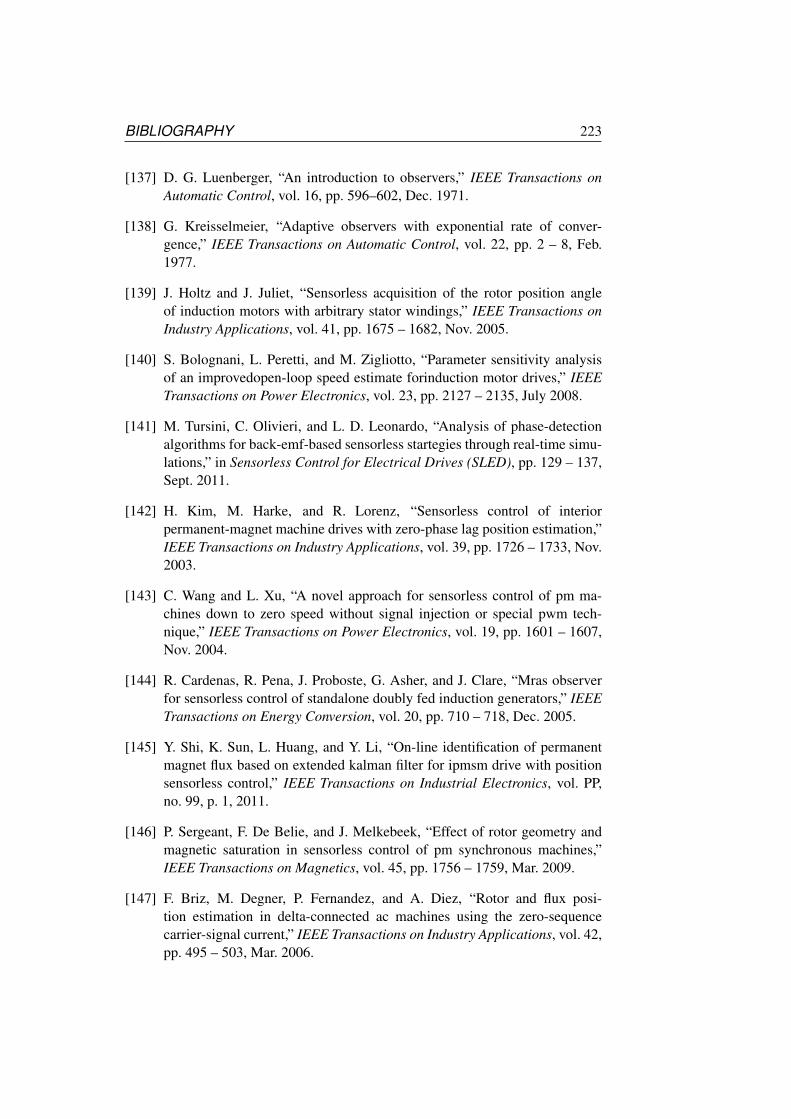
BIBLIOGRAPHY 223
[137] D. G. Luenberger, “An introduction to observers,” IEEE Transactions onAutomatic Control, vol. 16, pp. 596–602, Dec. 1971.
[138] G. Kreisselmeier, “Adaptive observers with exponential rate of conver-gence,” IEEE Transactions on Automatic Control, vol. 22, pp. 2 – 8, Feb.1977.
[139] J. Holtz and J. Juliet, “Sensorless acquisition of the rotor position angleof induction motors with arbitrary stator windings,” IEEE Transactions onIndustry Applications, vol. 41, pp. 1675 – 1682, Nov. 2005.
[140] S. Bolognani, L. Peretti, and M. Zigliotto, “Parameter sensitivity analysisof an improvedopen-loop speed estimate forinduction motor drives,” IEEETransactions on Power Electronics, vol. 23, pp. 2127 – 2135, July 2008.
[141] M. Tursini, C. Olivieri, and L. D. Leonardo, “Analysis of phase-detectionalgorithms for back-emf-based sensorless startegies through real-time simu-lations,” in Sensorless Control for Electrical Drives (SLED), pp. 129 – 137,Sept. 2011.
[142] H. Kim, M. Harke, and R. Lorenz, “Sensorless control of interiorpermanent-magnet machine drives with zero-phase lag position estimation,”IEEE Transactions on Industry Applications, vol. 39, pp. 1726 – 1733, Nov.2003.
[143] C. Wang and L. Xu, “A novel approach for sensorless control of pm ma-chines down to zero speed without signal injection or special pwm tech-nique,” IEEE Transactions on Power Electronics, vol. 19, pp. 1601 – 1607,Nov. 2004.
[144] R. Cardenas, R. Pena, J. Proboste, G. Asher, and J. Clare, “Mras observerfor sensorless control of standalone doubly fed induction generators,” IEEETransactions on Energy Conversion, vol. 20, pp. 710 – 718, Dec. 2005.
[145] Y. Shi, K. Sun, L. Huang, and Y. Li, “On-line identification of permanentmagnet flux based on extended kalman filter for ipmsm drive with positionsensorless control,” IEEE Transactions on Industrial Electronics, vol. PP,no. 99, p. 1, 2011.
[146] P. Sergeant, F. De Belie, and J. Melkebeek, “Effect of rotor geometry andmagnetic saturation in sensorless control of pm synchronous machines,”IEEE Transactions on Magnetics, vol. 45, pp. 1756 – 1759, Mar. 2009.
[147] F. Briz, M. Degner, P. Fernandez, and A. Diez, “Rotor and flux posi-tion estimation in delta-connected ac machines using the zero-sequencecarrier-signal current,” IEEE Transactions on Industry Applications, vol. 42,pp. 495 – 503, Mar. 2006.

224 BIBLIOGRAPHY
[148] P. Garcia, F. Briz, D. Reigosa, C. Blanco, and J. M. Guerrero, “On the useof high frequency inductance vs. high frequency resistance for sensorlesscontrol of ac machines,” in Symposium on Sensorless Control for ElectricalDrives (SLED), pp. 90 – 95, Sept. 2011.
[149] S.-C. Yang and R. D. Lorenz, “Comparison of resistance-based andinductance-based self-sensing controls for surface permanent-magnet ma-chines using high-frequency signal injection,” IEEE Transactions on Indus-try Applications, vol. 48, pp. 977 –986, May 2012.
[150] J. Moreira, “Indirect sensing for rotor flux position of permanent magnet acmotors operating over a wide speed range,” IEEE Transactions on IndustryApplications, vol. 32, pp. 1394 – 1401, Nov. 1996.
[151] S. Bolognani, S. Calligaro, R. Petrella, and M. Sterpellone, “Sensorless con-trol for ipmsm using pwm excitation: Analytical developments and imple-mentation issues,” in Symposium on Sensorless Control for Electrical Drives(SLED), pp. 64 – 73, Sept. 2011.
[152] S. Ogasawara and H. Akagi, “An approach to position sensorless drive forbrushless dc motors,” IEEE Transactions on Industry Applications, vol. 27,pp. 928 – 933, Sept. 1991.
[153] U.-H. Rieder, M. Schroedl, and A. Ebner, “Sensorless control of an exter-nal rotor pmsm in the whole speed range including standstill using dc-linkmeasurements only,” IEEE 35th Annual Power Electronics Specialists Con-ference, vol. 2, pp. 1280 – 1285, June 2004.
[154] F. De Belie, T. Vyncke, and J. Melkebeek, “Parameterless rotor positionestimation in a direct-torque controlled salient-pole pmsm without using ad-ditional test signals,” in International Conference on Electrical Machines(ICEM), pp. 1 – 6, Sept. 2010.
[155] P. Landsmann, D. Paulus, P. Stolze, and R. Kennel, “Saliency based encoder-less predictive torque control without signal injection,” in Power ElectronicsConference (IPEC), 2010 International, pp. 3029 –3034, June 2010.
[156] P. Landsmann, C. M. Hackl, and R. Kennel, “Eliminating all machineparameters in encoderless predictive torque control without signal injec-tion,” in International Electric Machines and Drives Conference (IEMDC),pp. 1259 – 1264, May 2011.
[157] J. Cai and Z. Deng, “Sensorless control of switched reluctance motor basedon phase inductance vectors,” IEEE Transactions on Power Electronics,vol. 27, pp. 3410 – 3423, July 2012.
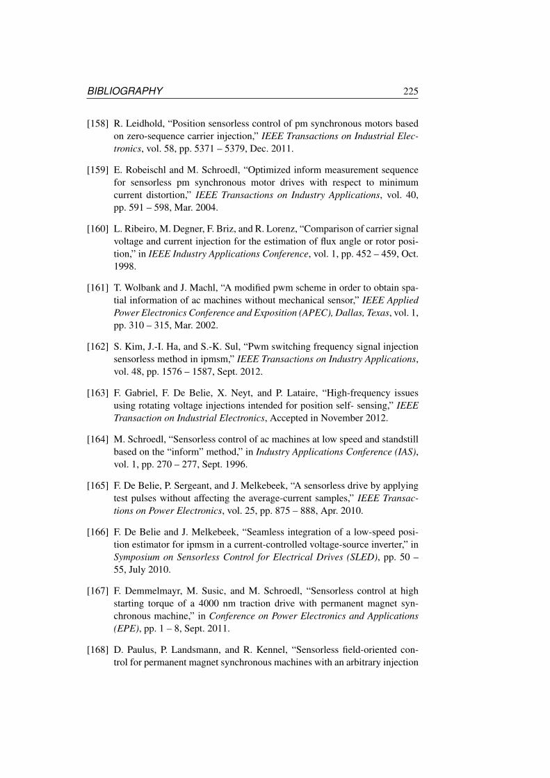
BIBLIOGRAPHY 225
[158] R. Leidhold, “Position sensorless control of pm synchronous motors basedon zero-sequence carrier injection,” IEEE Transactions on Industrial Elec-tronics, vol. 58, pp. 5371 – 5379, Dec. 2011.
[159] E. Robeischl and M. Schroedl, “Optimized inform measurement sequencefor sensorless pm synchronous motor drives with respect to minimumcurrent distortion,” IEEE Transactions on Industry Applications, vol. 40,pp. 591 – 598, Mar. 2004.
[160] L. Ribeiro, M. Degner, F. Briz, and R. Lorenz, “Comparison of carrier signalvoltage and current injection for the estimation of flux angle or rotor posi-tion,” in IEEE Industry Applications Conference, vol. 1, pp. 452 – 459, Oct.1998.
[161] T. Wolbank and J. Machl, “A modified pwm scheme in order to obtain spa-tial information of ac machines without mechanical sensor,” IEEE AppliedPower Electronics Conference and Exposition (APEC), Dallas, Texas, vol. 1,pp. 310 – 315, Mar. 2002.
[162] S. Kim, J.-I. Ha, and S.-K. Sul, “Pwm switching frequency signal injectionsensorless method in ipmsm,” IEEE Transactions on Industry Applications,vol. 48, pp. 1576 – 1587, Sept. 2012.
[163] F. Gabriel, F. De Belie, X. Neyt, and P. Lataire, “High-frequency issuesusing rotating voltage injections intended for position self- sensing,” IEEETransaction on Industrial Electronics, Accepted in November 2012.
[164] M. Schroedl, “Sensorless control of ac machines at low speed and standstillbased on the “inform” method,” in Industry Applications Conference (IAS),vol. 1, pp. 270 – 277, Sept. 1996.
[165] F. De Belie, P. Sergeant, and J. Melkebeek, “A sensorless drive by applyingtest pulses without affecting the average-current samples,” IEEE Transac-tions on Power Electronics, vol. 25, pp. 875 – 888, Apr. 2010.
[166] F. De Belie and J. Melkebeek, “Seamless integration of a low-speed posi-tion estimator for ipmsm in a current-controlled voltage-source inverter,” inSymposium on Sensorless Control for Electrical Drives (SLED), pp. 50 –55, July 2010.
[167] F. Demmelmayr, M. Susic, and M. Schroedl, “Sensorless control at highstarting torque of a 4000 nm traction drive with permanent magnet syn-chronous machine,” in Conference on Power Electronics and Applications(EPE), pp. 1 – 8, Sept. 2011.
[168] D. Paulus, P. Landsmann, and R. Kennel, “Sensorless field-oriented con-trol for permanent magnet synchronous machines with an arbitrary injection
226 BIBLIOGRAPHY
scheme and direct angle calculation,” in Symposium on Sensorless Controlfor Electrical Drives (SLED), pp. 41 – 46, Sept. 2011.
[169] F. Gabriel, F. De Belie, P. Druyts, X. Neyt, J. Melkebeek, and M. Acheroy,“Compensating the influence of the stator resistor and inverter nonlinear-ities in signal-injection based sensorless strategies,” in Vehicle Power andPropulsion Conference (VPPC), pp. 283 – 290, IEEE, Sept. 2009.
[170] K.-R. Cho and J.-K. Seok, “Induction motor rotor temperature estimationbased on a high-frequency model of a rotor bar,” IEEE Transactions on In-dustry Applications, vol. 45, pp. 1267 –1275, July 2009.
[171] S. Kellner and B. Piepenbreier, “Identification of ohmic stator resistancebased on low frequency current signal injection in permanent magnet syn-chronous machines,” in Power Electronics and Motion Control Conference,pp. T5–221 –T5–229, Sept. 2010.
[172] P. Champa, P. Somsiri, P. Wipasuramonton, and P. Nakmahachalasint, “Ini-tial rotor position estimation for sensorless brushless dc drives,” IEEE Trans-actions on Industry Applications, vol. 45, pp. 1318 – 1324, July 2009.
[173] S. Shan, L. Qingfu, X. Wei, and W. Xinghua, “A novel starting method forthe sensorless salient-pole brushless dc motors,” in Conference on ElectricalMachines and Systems (ICEMS), vol. 2, pp. 895 – 897, Aug. 2001.
[174] T. Noguchi, K. Yamada, S. Kondo, and I. Takahashi, “Initial rotor positionestimation method of sensorless pm synchronous motor with no sensitiv-ity to armature resistance,” IEEE Transactions on Industrial Electronics,vol. 45, pp. 118 – 125, Feb. 1998.
[175] H. Kim, K.-K. Huh, R. Lorenz, and T. Jahns, “A novel method for initialrotor position estimation for ipm synchronous machine drives,” IEEE Trans-actions on Industry Applications, vol. 40, pp. 1369 – 1378, Sept. 2004.
[176] T. J. S.-K. S. Yu-seok Jeong, R.D. Lorenz, “Initial rotor position estima-tion of an interior permanent-magnet synchronous machine using carrier-frequency injection methods,” IEEE Transactions on Industry Applications,vol. 41, pp. 38 – 45, Jan. 2005.
[177] P. Landsmann, D. Paulus, and R. Kennel, “Online identification of load an-gle compensation for anisotropy based sensorless control,” in Symposium onSensorless Control for Electrical Drives (SLED), pp. 80 – 84, Sept. 2011.
[178] Y. doo Yoon, S. ki Sul, S. Morimoto, and K. Ide, “High bandwidth sensorlessalgorithm for ac machines based on square-wave type voltage injection,”in Energy Conversion Congress and Exposition (ECCE), pp. 2123 – 2130,Sept. 2009.
BIBLIOGRAPHY 227
[179] H. Kim and R. Lorenz, “Carrier signal injection based sensorless controlmethods for ipm synchronous machine drives,” in Industry ApplicationsConference (IAS), vol. 2, pp. 977 – 984, Oct. 2004.
[180] J. Hu, J. Liu, and L. Xu, “Eddy current effects on rotor position estimationand magnetic pole identification of pmsm at zero and low speeds,” IEEETransactions on Power Electronics, vol. 23, pp. 2565 –2575, Sept. 2008.
[181] Y. doo Yoon and S. ki Sul, “Sensorless control for induction machines usingsquare-wave voltage injection,” in Energy Conversion Congress and Expo-sition (ECCE), pp. 3147 – 3152, Sept. 2010.
[182] C.-Y. Yu, J. Tamura, D. Reigosa, and R. Lorenz, “Position self-sensing eval-uation of a fi-ipmsm based on high frequency signal injection methods,” inEnergy Conversion Congress and Exposition (ECCE), pp. 3029 –3036, Sept.2011.
[183] W. Jianmin and G. Jianwei, “Analysis of position estimation error resultedfrom filter in carrier signal injection based sensorless control of pmsm,” inConference on Electrical Machines and Systems (ICEMS), pp. 1 – 6, Aug.2011.
[184] J.-H. Jang, J.-I. Ha, M. Ohto, K. Ide, and S.-K. Sul, “Analysis of permanent-magnet machine for sensorless control based on high-frequency signal in-jection,” IEEE Transactions on Industry Applications, vol. 40, pp. 1595 –1604, Nov. 2004.
[185] S.-C. Yang and R. Lorenz, “Surface permanent magnet synchronous ma-chine self-sensing position estimation at low speed using eddy currentreflected asymmetric resistance,” in Power Electronics and Applications(EPE), pp. 1 – 10, Sept. 2011.
[186] J.-H. Jang, S.-K. Sul, J.-I. Ha, K. Ide, and M. Sawamura, “Sensorless driveof surface-mounted permanent-magnet motor by high-frequency signal in-jection based on magnetic saliency,” IEEE Transactions on Industry Appli-cations, vol. 39, pp. 1031 – 1039, July 2003.
[187] S.-C. Yang and R. Lorenz, “Surface permanent-magnet machine self-sensing at zero and low speeds using improved observer for position, ve-locity, and disturbance torque estimation,” IEEE Transactions on IndustryApplications, vol. 48, pp. 151 – 160, Jan. 2012.
[188] F. De Belie and J. Melkebeek, “Application of a voltage adaptive sensor-less current controller to a multi-phase permanent-magnet synchronous ma-chine,” pp. 1 – 6, July 2009.

228 BIBLIOGRAPHY
[189] F. De Belie and J. Melkebeek, “Sensorless two-phase current control of afaulty three-phase salient-pole pmsm,” in International Conference on Elec-trical Machines and Systems (ICEMS), pp. 1 – 6, Nov. 2009.