Possible Spectrometer for eA Collider

 Seigo Kato

Faculty of Science, Yamagata University,

Yamagata 990-8560, Japan

  Presented to the workshop "Rare-Isotope Physics at Storage Rings"

February 3-8, 2002 at Hirschegg, Kleinwalsertal, Austria

• Requirements• Basic idea• Magnetic field• Expected performances• Size of dipole magnet• Merits and demerits• Spectrometer without the front counter• Conclusion

Contents

momentum resolution

10-4

angular resolution

1 mr

solid angle 40 msr

maximum momentum

800 MeV/c

momentum range 10 %

minimum angle 6 o

colliding length acceptance

10 cm

Requirements to the collider spectrometer

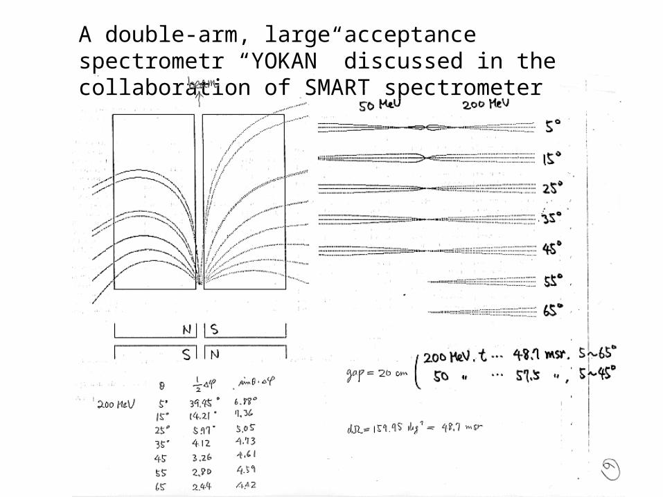
A double-arm, large acceptance spectrometr “YOKAN” discussed in the collaboration of SMART spectrometer

Possible spectrometers which do not deflect nor stop the beam

1. Conventional spectrometers at the nearest approach to the beam

MAMI-C(6o), JLAB(12o-->6o with septums)

2. Spectrometers in which beams go straight due to special conditions.

2-1 Uniform solenoid field

along the field line ---> B // p

conventional collider spectrometers

2-2 Quadrupole field

along the symmetric axis ---> B = 0

“YOKAN” spectrometer

Basic idea of the Q-magnet-based spectrometer

• Electron and RI beams collide each other along the symmetry axis of the quadrupole magnet of the spectrometer.

• Intact beams go straight along the field-free, symmetrical axis of the quadrupole magnet.

• Scattered electron are focused vertically, magnifying the acceptance.

• They are horizontally defocused, magnifying the angle of exit.

Electrons are extracted from the side face of the quadrupole magnet.

Electrons scattered to extreme forward angles can be analyzed.

• They are then analyzed by a dipole magnet.

• The exit angle from the quadrupole magnet is almost constant.

• (demerit) We lose significant part of the information on scattering angles.

• (merit) The scattering angle can be changed without rotating the dipole magnet if we adjust the strength of the quadrupole magnet and/or the colliding position of the beams.

Possibilities to change the detection angle

1. Move the dipole magnet parallel to the beam line

--- It may be easier than the rotation .

2. Adjust the collision point and Q-magnet strength

3. Adjust only the Q-magnet strength

4. Enlarge the horizontal angular acceptance

100~300 mr 300~500 mr

Change the detection angle by beam and Q-magnet

Strength of the Q-magnet and the colliding position are adjusted

20 ~ 100 mr780 ~ 880 mr

reversed polarity

Extreme forward and extreme backward angles

100~300 mr 300~500 mr

Change the detection angle only by Q-magnet

merit: fixed collision position

demerit: reduced horizontal acceptance

100~500 mr

Cover the necessary angular range with one shot

Counter resolution 0.2 mmMultiple scattering 0.5 mr

Counter resolution 0.1 mmMultiple scattering 0.2 mr

Resolutions

Dependence on the colliding length

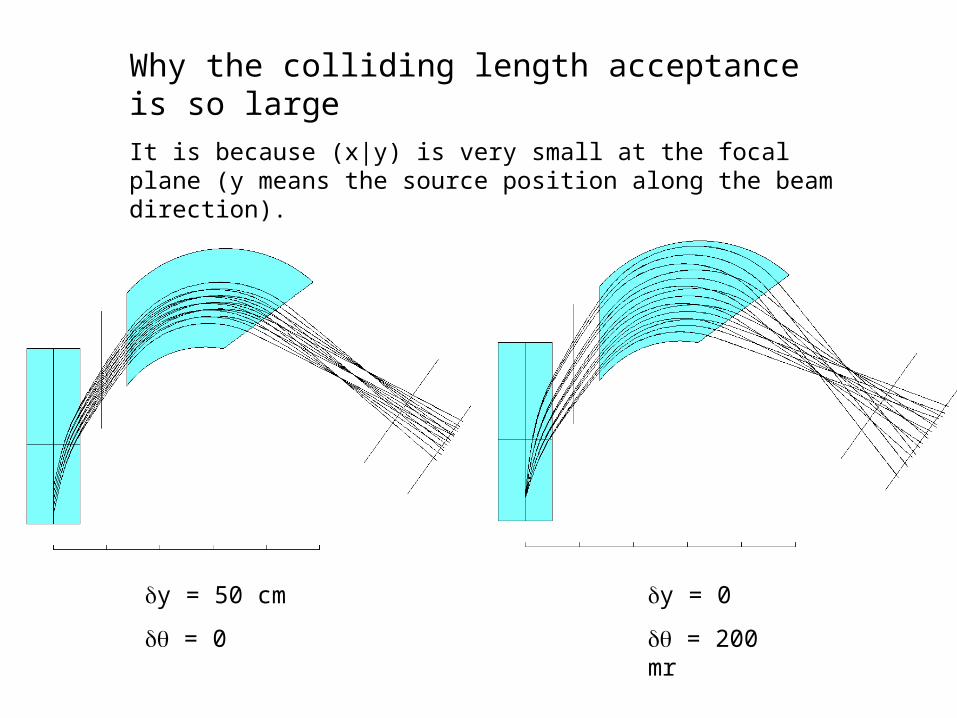
Why the colliding length acceptance is so large

It is because (x|y) is very small at the focal plane (y means the source position along the beam direction).

y = 50 cm

= 0

y = 0

= 200 mr

From traditional to precise expression of fringing field

55

44

33

2210

)exp(1

1)(

scscscscsccS

Ssh

Traditional method (J.E.Spencer & H.A.Enge: NIM 49(1967)181)

Define s = x / G and fit By along x-axis by

.

0 if 0

....]!3

[),(

....]!2

)([

.....!2

)0,(),(

2

3

33

0

2

22

0

2

22

jB

dx

hdy

dx

dhyByxB

dx

hdyxhB

y

ByxByxB

x

yyy

Extension to two-dimensional space :

Field strength distribution

From the field calculation

From the parameters

up to 2-nd order

We need precise value up to y = G/2.

There is no reason to justify the cut-off at the 2-nd order term.

Can we sum up to infinity?

)](Im[),(

)](Re[

)]()Re[exp()()cos(

....]!6!4!2

)([

.....!6!4!2

)0,(),(

0

0

00

6

66

4

44

2

22

0

6

66

4

44

2

22

iyxhByxB

iyxhB

xhx

iyBxhdx

dyB

dx

hdy

dx

hdy

dx

hdyxhB

y

By

y

By

y

ByxByxB

x

yyyyy

Exact summation up to infinity.

If the field is independent of the z-coordinate

There is no reason to terminate the summation at a finite order when the exact summation is possible.

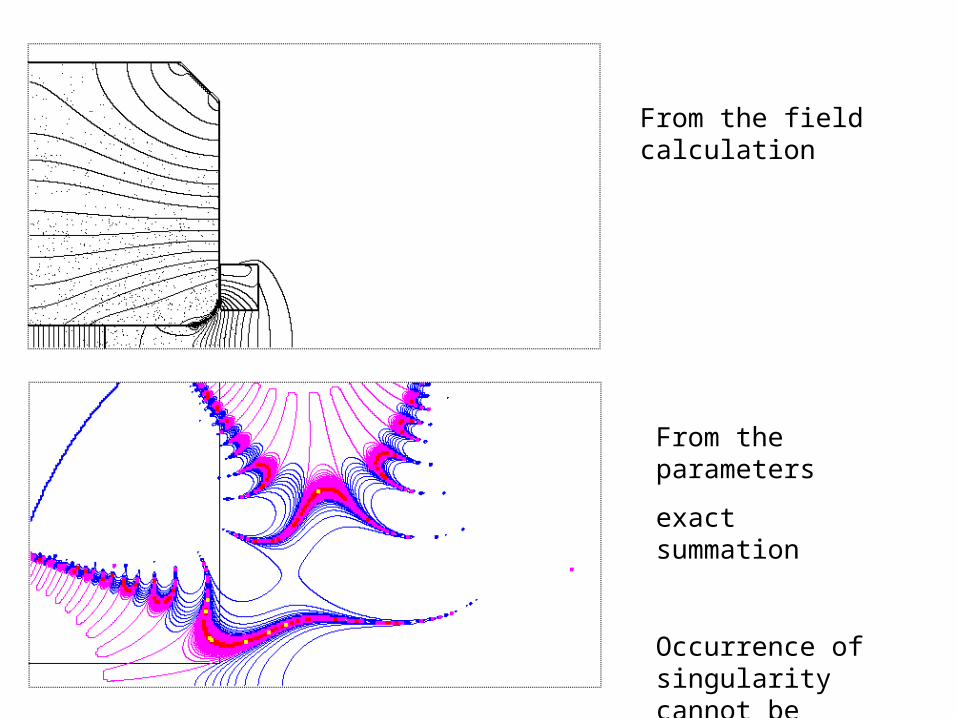
From the parameters

exact summation

Occurrence of singularity cannot be avoided.

From the field calculation

Occurrence of singularities in two-dimensional space

For complex S, exp(S) = -1 is possible.

We have to know the location of singularities by solving following equation:

)12(55

44

33

2210 imscscscscscc

(generally unsolvable)

G

yi

G

xs

scscscscsccS

Ssh

55

44

33

2210

)exp(1

1)(

Enge’s long-tail parameter set gives strange field

Up to 2-nd order Up to infinite order

A new fitting function

G

yi

G

xs

location of singularities

n

a

bssh

)]exp(1[

1)(

,...5 ,3 ,y

aGaGaG

bGx

16.02

1

0

a

b

safety condition

Enge’s short tail parameter set gives ….

original parameters parameters converted

)](Re[),(

)](Im[),(

definingby

space full toextended be can fitting The

.

a variable withaxis- along )0,( to

)]exp(1[

])1(1[2

11

)1()(

fittingby extracted wereParameters

0

0

2

shByxB

shByxBG

yi

G

xs

G

xs

xxBa

bs

dcscsesh

y

x

y

n

Field of the quadrupole magnet

standard 20 msr version

slim 10 msr version

100~200 mr 200~300 mr

300~400 mr 400~500 mr

Pair spectrometer 1

same polarity

Pair spectrometer 2

opposite polarity

Specification of the magnets

quadrupole magnet

gap of quadrupoles 32 cm

gap of dipoles 10 cm

field gradient 6 T/m

maximum field 1.5 T

mass 30 ton

dipole magnet

maximum field 1.4 T

gap 24 cm

mass 280 ~ 540 ton

power consumption 520 ~ 410 kW

Comparison with existing spectrometers

type conventional cylindrical Q-magnet based

example MAMI-B OPAL present

target fixed beam beam

mom. resolution high low high

colliding length

acceptance

5 cm

(dipole gap)

~ 1 m

(vertex counter)

10 cm

magnet D solenoid QD

focal plane exists do not exist exists

symmetry vertical plane beam axis horizontal plane

solid angle 5.6 msr ~ 4sr 10~20 msr

minimum angle 7o ? 1o

Merits and demerits of the present spectrometer

merits• high resolution

• extreme forward angle

• large acceptance of 　　colliding length

• no need of the rotation

• existence of focal plane

• horizontal median plane

• simple structure

demerits • interference with the beam

• poor resolution of horizontal angle

• angle dependence of focusing property

• no defining slit

Can we improve the horizontal angular resolution by removing the front counter which causes the serious multiple scattering?

mr 80

mr 200mr 100

removal of the front counter

decrease of momentum resolution

necessity of dispersion increase

increase of bending angle

decrease of horizontal acceptance

necessity of increasing the vertical angle acceptance

large gap of quadrupole magnet

Dependence of resolutions on the beam length and on the vertical angle

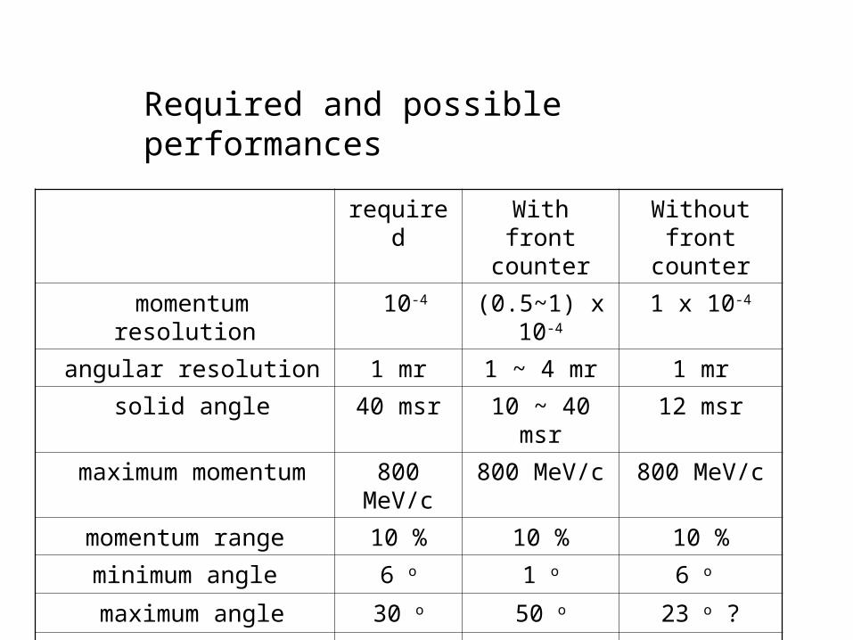
Required and possible performances

required With front counter

Without front counter

momentum resolution 10-4 (0.5~1) x 10-4 1 x 10-4

angular resolution 1 mr 1 ~ 4 mr 1 mr

solid angle 40 msr 10 ~ 40 msr 12 msr

maximum momentum 800 MeV/c 800 MeV/c 800 MeV/c

momentum range 10 % 10 % 10 %

minimum angle 6 o 1 o 6 o

maximum angle 30 o 50 o 23 o ?

colliding length acceptance 10 cm 10 ~ 50 cm < 10 cm

Conclusion

The spectrometer equipped with the front counter has many advantages.

- The momentum resolution is enough.

- More than enough angular range can be accepted without rotation.

- More than enough colliding length can be accepted.

- The structure is very simple.

The most serious disadvantage is the poor angular resolution.

It can be improved by removing the front counter and by losing some of the advantages.

The choice depends on the counter development, the beam development, and the requirement of the physics.

Ray-tracing calculation for designing a magnetic spectrometer

2. Trace rays by solving the equation of motion

with appropriate initial conditions.

Bvr

qdt

dm

2

2

3. Evaluate the optical properties at the counter position.

image sharpness, momentum sensitivity, etc.

1. Prepare magnetic field distribution.

It has to be as realistic as possible.

Field line and field strength distributions of BBS-Q1 magnet

Momentum resolution of a spectrometer

n)(aberratioification)size)(magn (beam

dispersion

counterat size image beam

counterat separationresolution

aberration elimination: hardware correction vs software correction