Post-Treatment Assessment of Fracture Networks

M. Gonzalez, A. Dahi Taleghani, P. Puyang and J. Lorenzo, Louisiana State University, J. Le Calvez, Schlumberger

Abstract

An integrated modeling methodology is proposed to generate a network of potential paths for hydraulic fracture growth in naturally fractured reservoirs based on formation properties and recorded microseismic maps. !e generated network can be further used for forward fracturing simulations to determine the geometry and height growth of induced fractures, as well as proppant transports in the fracture network. Microseismic map is used to generate the network of pre-existing natural fractures to provide a more reliable map of induced fracture network. For di"erent realizations of natural fracture distributions generated by computer simulations, cohesive interface technique is used to model the evolution of complex fracture networks.

In the past few years, improvements in hydraulic fracturing technology contributed signi#cantly to the spikes in gas production in the United States by creating conductive $ow paths from the reservoir to the wellbore (USEIA report, 2009). Production from unconventional shale gas reservoirs has relied heavily on this technology. As such, research e"orts now center on how to achieve the optimal fracture design with known reservoir characteristics, or at least improving fracturing treatment design. !e preliminary step in assessing any hydraulic fracturing job is identifying the geometry of induced fractures. Accurate prediction of the fracture network geometry is a desirable objective yet rarely accomplished with modern fracturing technology. A model that is able to predict the geometry and evolution pattern of every individual fracture in the fracture network barely exists due to the fact that it is essentially impossible to collect every detail regarding individual fractures. It is also notable that although natural fractures may exist in a wide range of length and widths (Ortega et al. 2006), here we are mainly interested in natural fractures with comparable size with hydraulic fractures. Small natural fractures may also open due to thermal stresses (Dahi Taleghani et al. 2013a) or residual plastic deformations (Dahi Taleghani et al. 2013b); since they will not a"ect the direction of fracture propagation, we will ignore them here although they could a"ect the initial hydrocarbon production rate. !erefore, we set our objective to develop an optimal approach to describe the seemingly unmanageable spatio-temporal evolution of fracture patterns. While traditional models assuming simple symmetric wing or bi-wing type fracture networks are commonly appropriate for ideal homogenous reservoirs, they are inadequate in representing the complex nature of the fracture network in reservoirs with pre-existing natural fractures. Historically, pressure diagnostics (Nolte and Smith 1979, Nolte 1991) and tiltmeter measurements (Warpinski et al. 1997) were the main tools for estimating fractures’ geometry. Initial steps in pressure analysis include pressure data collection and processing; important information about formation, fracture and treatment may be obtained by identifying general pressure variation patterns, which are similar to methods used in pressure transient analysis. Economides and Nolte (2000) have provided a complete review of classic pressure diagnostic techniques to infer critical parameters of the fracturing treatment, including fracture geometry, closure pressure, fracture height growth, formation pressure capacity, treatment e%ciency, and $uid $ow

patterns. !is approach has gained its popularity in early 1990’s because pressure data is the least costly piece of information to collect in the #eld, and this method was providing acceptable predictions for massive fracturing jobs in vertical well. Utilization of hydraulic fracturing to stimulate new developments in low permeability, naturally fractured formations like Barnett shale, which was frequently done in multiple stages through horizontal wells, posed new challenges in interpreting treatment pressure data. With the introduction of hydraulic fracturing into shale plays, which were usually naturally fractured, interactions between natural fractures and hydraulic fractures lead to the formation of complicated network of induced fractures.

In addition to the pressure analysis technique, microseismic data also helps in evaluating the e"ectiveness of the treatment design. Due to the complexity of data interpretation and associated cost, microseismic technology is still considered an expensive and more descriptive analysis tool. Because of the inherent properties of microseismic waves (i.e., low frequency and high noise to signal ratio), resolution in locating microseismic events cannot be better than 50 &. (Maxwell, 2008). !is limits the application of microseismic mapping method to direct measurement of fracture spacing or intersection of fractures. Tiltmeters could not be an e"ective technique for the system of multiple fractures. Microseismic data collected during hydraulic fracturing treatments for Barnett Shale wells reveals complex fracture geometries, where hydraulic fractures may propagate as multiple segments with di"erent orientations in$uenced by pre-existing natural fractures, which lead to a cloud of event epicenters. Although microseismic mapping provides insights on the interaction of hydraulic fractures with natural fracture systems and formation stress regimes (Li et al. 1998), the phenomenon behind the scattered epicenters observed during fracture jobs were not fully explained (Rutledge and Phillips, 2003). Waters et al. (2006) provided a map of the microseismic events generated during a stage of hydraulic fracturing treatment. !e microseismic map did not show a narrow band of events perpendicular to the minimum horizontal stress, but there was a huge region of a"ected rock volume, extending hundreds to thousands of feet along the expected propagation direction of hydraulic fractures (parallel to the orientation of maximum horizontal stress). !e cloud also extended hundreds of feet in the orthogonal direction. Such #ndings con#rmed the presence of a complex fracture network. !e main mechanism for developing a

Introduction

Peer Reviewed

complex fracture pattern is the interaction between natural fractures and hydraulic fractures. One of the decisive factors in determining the geometry of the induced hydraulic fractures is the characteristics of the pre-existing natural fractures, and other formation properties that in$uence the fracture pattern, including in-situ stress state, permeability and mechanical properties, are also closely related to the existence of natural fractures.

Occasionally, interactions between natural fractures and hydraulic fractures are investigated through laboratory experiments, and results have shown that di"erent parameters, especially di"erential stress, govern the interactions between natural and hydraulic fractures (Warpinski, and Teufel, 1987). Further laboratory investigations con#rmed the formation of complicated fracture networks in the presence of natural fractures. Je"ery et al. (2009) conducted mineback #eld experiments to examine the growth of hydraulic fractures through a system of natural fractures. In such situations, the induced fracture tend to develop in a much complicated way due to the diversion of progressing hydraulic fracture into natural fractures, or simply the opening these fractures (Warpinski and Teufel, 1987; Olson and Dahi Taleghani, 2009, Dahi Taleghani and Olson, 2013). !is complexity can either be suppressed or utilized in some extent to bene#t the reservoir productivity (Cipolla et al, 2010). Considering the fact that all pressure diagnostic techniques were built by considering induced hydraulic fractures as a single-strand fracture, they are not reliable to interpret pressure data of a network of fractures.

In summary, tiltmeters and microseismic monitoring do not have su%cient resolution to identify small scale fracture complexity. However, it is possible to gather some qualitative data about far-#eld fracture complexity from fracture pressure analysis (Cipolla et al. 2008) and core studies. In an ideal approach, microseismic data in combination with other resources (e.g. pump data or bottomhole pressure) may provide better understanding of the characteristics of induced fractures. Having access to such integrated models can strongly in$uence future completion design and overall #eld development strategy. Of course, this integrated analysis would only be possible by incorporating pressure analysis for a system of multiple interacting fractures. Except for single fracture situation, pressure evolution in multiple fracture problems cannot be addressed with analytical solutions and requires detailed numerical analyses.

Cipolla et al. (2010) discussed how fracture network complexity may change bottomhole pressure during the treatment as well as future production in comparison to the cases with single induced fracture. !rough reservoir simulation, they claimed that fracture conductivity required to maximize production is proportional to the square root of fracture spacing, thus fracture complexity is inversely proportional to the fracture conductivity requirement. Moreover, they argued that in complicated fracture networks, the average proppant concentration will become insigni#cant, and therefore proppant placement is less likely to impact the well performance.

Due to the limited access to the subsurface, modeling or so-called numerical experiments on di"erent realizations of natural fractures, which have the same overall statistical properties measured in outcrops, could be a reasonable tool to predict potential pathways for fracturing $uid $ow in the subsurface or correlate bottomhole pressure changes. Xu et al. (2010) tried to address this issue by proposing a semi-analytical

pseudo 3-D fracturing simulator to simulate the growth of hydraulic fracture networks (HFN) in the grid of equally-spaced natural fractures. !eir wiremesh model assumed a growing symmetric elliptical front for the development of induced fracture network. However, spatial and temporal distributions of microseismic events mapped during many fracturing treatments had revealed asymmetric and preferential direction for fracture propagation. !e presence of major or pre-existing natural fractures and their orientation could play a key role in the development of fracture networks in di"erent directions. Fluid pressure and injection rate have been used for a long time to estimate fracture geometries. However, due to the complex geometry of induced fracture networks, these methods are not applicable in reservoirs with pre-existing natural fractures. To #ll this gap, a set of realizations of mathematically equivalent fracture networks are developed here to represent the geometry of natural fracture network. In developing the equivalent networks, the assumptions of having perpendicular fracture sets and their alignment with the principal in situ stresses are relaxed. HFN realizations are not only constrained by the injection rate and the total mass of injected $uid, but also relate to temporal and spatial distribution of mapped microseismic events to honor the measured bottomhole treatment pressure. Integrating microseismic events into the analysis requires a sophisticated #ltering process to reduce the interference of microseismic events that are not generated along the hydraulically induced fractures. For instance, some of these events might have been induced by the reactivation of fractures in the vicinity of stimulated zone. !is mathematical model incorporates treatment pressure, injection rate, general characteristic of natural fractures, and formation mechanical properties to obtain HFN geometrical parameters. !e proposed methodology is utilized in a multi-stage stimulation exercises in Barnett Shale wells. Simulated HFN using this technique is compared with the HFN produced using Xu et al. (2010) technique. Production data forecasted based on these fracture networks is compared at the end as the validation for the proposed technique. We show how location of mapped microseismic events may serve as a useful piece of data in combination with pressure analysis in predicting the geometry of the hydraulically-induced fracture network.

Hydraulic fractures interactions with natural fractures

!e size of natural fractures ranges from few millimeters (tiny #ssures) to several thousand meters (faults). As opposed to natural fractures, hydraulic fractures are created arti#cially with the force of injected pressurized $uid. By generating a hydrostatic pressure that exceeds the minimum in-situ stress of the formation, fractures are opened up in a direction perpendicular to that of smallest resistance, i.e. minimum principal stress.

Improved hydrocarbon production does not necessarily rely on hydraulic fracturing. In some cases, natural fractures may also contribute to the recovery of oil and gas. Natural fractures in formations with moderate permeability can serve as the $ow path for hydrocarbons as well, and the presence of natural fractures may facilitate the formation of a network of induced fractures. On the other hand, natural fractures may also negatively impact hydraulic fracturing treatment by causing extensive leako" and reduced $ow back (Warpinski, 1990). A large population of natural fractures in the subsurface is cemented by digenetic materials. Although they will not increase overall permeability initially, opening of these natural fractures will increase drainage area tremendously.

Fortunately in most cases, these natural fractures act as weak paths for fracture growth. !erefore if they are aligned in a favorable direction with in situ tectonic stresses, there is a good likelihood that these natural fractures can be opened during treatment (Gale et al. 2007, Dahi Taleghani and Olson, 2011). !e intersections of natural fractures with hydraulic fractures result in irregular fracture patterns, including non-planar fractures or fracture branching. On one hand, opening of these natural fractures improves productivity of the formation; on the other hand, coalescence of these fractures into hydraulic fractures makes pressure analysis and prediction of fracture growth quite complicated. Overall, interactions between natural fractures and hydraulic fractures make the fracturing design and execution more challenging. Investigation and understanding of their interaction are crucial in achieving successful fracture treatment in formations with natural fracture network.

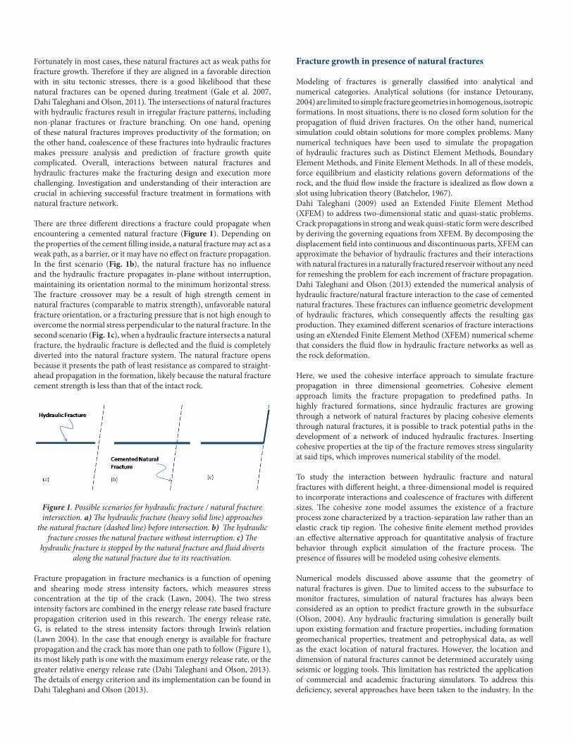
!ere are three di"erent directions a fracture could propagate when encountering a cemented natural fracture (Figure 1). Depending on the properties of the cement #lling inside, a natural fracture may act as a weak path, as a barrier, or it may have no e"ect on fracture propagation. In the #rst scenario (Fig. 1b), the natural fracture has no in$uence and the hydraulic fracture propagates in-plane without interruption, maintaining its orientation normal to the minimum horizontal stress. !e fracture crossover may be a result of high strength cement in natural fractures (comparable to matrix strength), unfavorable natural fracture orientation, or a fracturing pressure that is not high enough to overcome the normal stress perpendicular to the natural fracture. In the second scenario (Fig. 1c), when a hydraulic fracture intersects a natural fracture, the hydraulic fracture is de$ected and the $uid is completely diverted into the natural fracture system. !e natural fracture opens because it presents the path of least resistance as compared to straight-ahead propagation in the formation, likely because the natural fracture cement strength is less than that of the intact rock.

Figure 1. Possible scenarios for hydraulic fracture / natural fracture intersection. a) !e hydraulic fracture (heavy solid line) approaches

the natural fracture (dashed line) before intersection. b) !e hydraulic fracture crosses the natural fracture without interruption. c) !e

hydraulic fracture is stopped by the natural fracture and "uid diverts along the natural fracture due to its reactivation.

Fracture propagation in fracture mechanics is a function of opening and shearing mode stress intensity factors, which measures stress concentration at the tip of the crack (Lawn, 2004). !e two stress intensity factors are combined in the energy release rate based fracture propagation criterion used in this research. !e energy release rate, G, is related to the stress intensity factors through Irwin’s relation (Lawn 2004). In the case that enough energy is available for fracture propagation and the crack has more than one path to follow (Figure 1), its most likely path is one with the maximum energy release rate, or the greater relative energy release rate (Dahi Taleghani and Olson, 2013). !e details of energy criterion and its implementation can be found in Dahi Taleghani and Olson (2013).

Fracture growth in presence of natural fractures

Modeling of fractures is generally classi#ed into analytical and numerical categories. Analytical solutions (for instance Detourany, 2004) are limited to simple fracture geometries in homogenous, isotropic formations. In most situations, there is no closed form solution for the propagation of $uid driven fractures. On the other hand, numerical simulation could obtain solutions for more complex problems. Many numerical techniques have been used to simulate the propagation of hydraulic fractures such as Distinct Element Methods, Boundary Element Methods, and Finite Element Methods. In all of these models, force equilibrium and elasticity relations govern deformations of the rock, and the $uid $ow inside the fracture is idealized as $ow down a slot using lubrication theory (Batchelor, 1967).Dahi Taleghani (2009) used an Extended Finite Element Method (XFEM) to address two-dimensional static and quasi-static problems. Crack propagations in strong and weak quasi-static form were described by deriving the governing equations from XFEM. By decomposing the displacement #eld into continuous and discontinuous parts, XFEM can approximate the behavior of hydraulic fractures and their interactions with natural fractures in a naturally fractured reservoir without any need for remeshing the problem for each increment of fracture propagation. Dahi Taleghani and Olson (2013) extended the numerical analysis of hydraulic fracture/natural fracture interaction to the case of cemented natural fractures. !ese fractures can in$uence geometric development of hydraulic fractures, which consequently a"ects the resulting gas production. !ey examined di"erent scenarios of fracture interactions using an eXtended Finite Element Method (XFEM) numerical scheme that considers the $uid $ow in hydraulic fracture networks as well as the rock deformation.

Here, we used the cohesive interface approach to simulate fracture propagation in three dimensional geometries. Cohesive element approach limits the fracture propagation to prede#ned paths. In highly fractured formations, since hydraulic fractures are growing through a network of natural fractures by placing cohesive elements through natural fractures, it is possible to track potential paths in the development of a network of induced hydraulic fractures. Inserting cohesive properties at the tip of the fracture removes stress singularity at said tips, which improves numerical stability of the model.

To study the interaction between hydraulic fracture and natural fractures with di"erent height, a three-dimensional model is required to incorporate interactions and coalescence of fractures with di"erent sizes. !e cohesive zone model assumes the existence of a fracture process zone characterized by a traction-separation law rather than an elastic crack tip region. !e cohesive #nite element method provides an e"ective alternative approach for quantitative analysis of fracture behavior through explicit simulation of the fracture process. !e presence of #ssures will be modeled using cohesive elements.

Numerical models discussed above assume that the geometry of natural fractures is given. Due to limited access to the subsurface to monitor fractures, simulation of natural fractures has always been considered as an option to predict fracture growth in the subsurface (Olson, 2004). Any hydraulic fracturing simulation is generally built upon existing formation and fracture properties, including formation geomechanical properties, treatment and petrophysical data, as well as the exact location of natural fractures. However, the location and dimension of natural fractures cannot be determined accurately using seismic or logging tools. !is limitation has restricted the application of commercial and academic fracturing simulators. To address this de#ciency, several approaches have been taken to the industry. In the

#rst approach, a fully random set of fractures are considered as natural fractures, and hydraulic fracture is assumed to only propagate through these fractures (Meyer and Brazan, 2011), which is not completely representing the actual fracture distribution in the formation of interest. Extensive outcrop studies in the last couple of decades demonstrate that joints distribution is not fully random distribution; depending on the rock properties and tectonic history, it may range from a single set of parallel joints to multiple sets of intersecting joints (Ortega et al. 2000, Ortega et al. 2006). Additionally, depending on formation properties, each joint set could be equally spaced or clustered (Olson et al. 2008). In summary, the pattern of induced fracture networks is dictated by natural fractures and their orientation with respect to principal in situ stresses. !erefore, we need to set our goal to speculate the characteristic geometry of natural fractures in the subsurface rather than a deterministic approach of determining the exact location of each fracture as this problem is ill-conditioned and does not have a unique solution.

Any non-deterministic approach requires acquiring a forward model to simulate hydraulic fracture propagation for di"erent realizations of natural fractures. !erefore, it is expected that the forward model be quick enough to include numerous natural fracture realizations, capable of modeling the true mechanics of hydraulic fracture and natural fractures intersections, and model di"erent natural fracture geometries with least costly meshing techniques. We found cohesive element approach a suitable tool for this technique.

Cohesive element technique

Cohesive zone model assumes the existence of a fracture zone characterized by a traction-separation law. !e pre-de#ned surface is made up of elements that support the cohesive zone traction-opening calculation embedded in the rock, and the hydraulic fracture will grow along this surface. !e fracture process zone (unbroken cohesive zone) is de#ned within the separating surfaces where the surface tractions are nonzero (see Figure 2).

Figure 2. Embedded cohesive zone at the tip of a hydraulic fracture. Two zones can be identi#ed: i) broken cohesive zone where

tractionseparation law is no longer e$ective, and ii) unbroken cohesive zone where tranction separation law is working.

!ere are three failure mechanisms taken into account in fracture modeling: i) fracture initiation criterion, ii) fracture evolution law, and iii) choice of element removal upon reaching a completely damaged state. Fracture Initiation Criterion is referred to as the beginning of degradation due to stresses and/or strains satisfy certain damage initiation criteria that were speci#ed. !ere are many fracture initiation criterion in ABAQUS. It could be assumed that initiation begins when

maximum nominal, quadratic stress ratio, maximum nominal strain, or quadratic strains reached their critical values. Fracture Evolution Law Criterion is usually implemented that the fracture propagates when the stress intensity factor at the tip exceeds the rock toughness. When the interface thickness is negligibly small, it may be straightforward to de#ne the constitutive response of the cohesive layer directly in terms of traction versus separation.

D=0 D=1

tn0

tn

kn0kn

įn0 įnf įn

Gn

Gf

ts/ttts0/tt0

- įs0/įt0

- įsf/įtf- įs0/įt0

- ts0/tt0

Gs/Gtks0/kt0

ks/kt

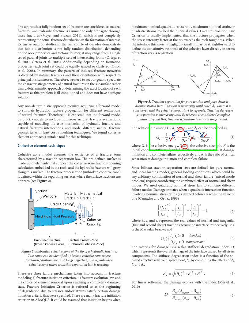
Figure 3. Traction-separation for pure tension and pure shear is deomonstrated here. Traction is increasing until reach δo, where it is

considered that the cohesive layers start to separate. Traction decreases as separation is increasing until δf, where it is considered complete

failure. Beyond this, traction separation law is not longer valid.

!e relationship among Gc, K, Tmax, δo, and δf can be described as

(1)

where Gc is the cohesive energy, Tmax is the cohesive strength, K is the initial cohesive sti"ness, δo and δf are the critical separation at damage initiation and complete failure respectively, and δo is the ratio of critical separation at damage initiation and complete failure.

Since bilinear traction-separation laws are de#ned for pure normal and shear loading modes, general loading conditions which could be any arbitrary combination of normal and shear failure (mixed mode problem) require considering the combined e"ect of normal and shear modes. We used quadratic nominal stress law to combine di"erent failure modes. Damage initiates when a quadratic interaction function involving nominal stress ratios (as de#ned below) reaches the value of one (Camacho and Ortiz,, 1996)

(2)

where tn, ts and tt represent the real values of normal and tangential (#rst and second shear) tractions across the interface, respectively. < > is the Macaulay bracket and

(3)

!e metrics for damage is a scalar sti"ness degradation index, D, which represents the overall damage of the interface caused by all stress components. !e sti"ness degradation index is a function of the so-called e"ective relative displacement, δm by combining the e"ects of δt, δs and δn,

(4)

For linear so&ening, the damage evolves with the index (Mei et al., 2010)

(5)

G T TTKc f f ff= = =

12

12 20

2

δα

δα

,

tt

tt

tt

n

n

s

s

t

t0

2

0

2

0

2

1

+

+

= ,

t t ttn

n t

n

,,

≤<

00 0

(tension)

(compression),

δ δ δ δm n s t= + +2 2 2

D mf m m

m mf m

=−

−

δ δ δδ δ δ( )( ),max

,max

0

0

.

where δm,max is the maximum e"ective relative displacement attained during the loading history. δm0 and δmf are e"ective relative displacements corresponding to δn0 and δs0, and δnf and δsf are shown in Figure 3. For nonlinear mechanics, the most robust criterion is described by the constitutive model of the cohesive zone proposed by Barenblatt (1962) and Hillerborg (1976). !is law assumes that the cohesive surfaces are intact without any relative displacement, and exhibit reversible linear elastic behavior until the traction reaches the cohesive strength or equivalently the separation exceeds δ0. Beyond this value, the traction reduces linearly to zero up to δf. Figure 4 shows how crack openings provide paths for tangential and normal $ow inside the fracture. !e $uid leako" is normal $ow. !e tangential $ow within the gap is governed by the lubrication equation (Batchelor, 1967), which is a combination of Poiseuille’s $ow

(6)

and the continuity equation

(7)

Figure 4. Two type of "ows inside the fracture: i) tangential "ow, which contribute to fracture opening, and ii) normal "ow, which is the "uid

that will be lost in the formation (better known as leak-o$).

In the above equation, q(x,y,t) is the $uid $ux in tangential direction, is the $uid pressure gradient along the cohesive zone, w(x,y,t) is the crack opening, μ and Q(t) are $uid viscosity and injection rate, respectively. !e qt(x,y,t) and qb(x,y,t) terms are the normal $ow rates into the top and bottom surfaces of the cohesive elements, respectively. !e normal $ow rates are de#ned as

(8)

(9)

where pf and pb are the pore pressures in the adjacent pore-$uid (poroelastic) material on the top and bottom surfaces of the fracture, respectively, and ct and cb de#ne the corresponding $uid leako" coe%cients. !is problem can be approximated numerically using standard Galerkin formulation for Finite element methods (Lewis and Schre'er, 2000). !e equation in matrix notation can be written as the following:

(10)

where u are nodal displacements, p are nodal pressures, F are nodal forces, q are nodal $uxes, [K] is the sti"ness matrix, [L] is the coupling matrix, [H] is the $ow matrix and [S] is the compressibility matrix. !e #rst equation of equations (10) is the sti"ness equation and the second equation is $ow equation. Unknown variables u and p are substituted by their nodal values and the interpolation functions (shape functions). !e de#nition of matrices used in equation (10) are given below (Lewis and Schre'er, 2000)

(11)

where D is the elasticity matrix, NP and Nu are shape functions for pressure and displacements, respectively. !e parameter is de#ned

as .

To validate the numerical model, a two-dimensional #nite element model is built in ABAQUS for a single fracture. !e reservoir size is assumed to be much larger than the dimension of hydraulic fracture and is modeled with quadratic plane strain elements. Injection well is considered to be at the center of the model, and a layer of cohesive elements is passing through the injection well, which represents the possible path for the hydraulic fracture and is consisted of 6-node cohesive elements. !e initial length of the hydraulic fracture, 22 m (Figure 5), is set to be much smaller than the model size to avoid any boundary e"ect. !e right and le& faces are constrained in x-direction and upper and lower faces were constrained in y-direction as boundary conditions. !e in-situ stresses are de#ned as initial stresses to avoid any excessive deformation in the initial equilibration process. !e mechanical properties utilized to build this model are listed in Table 1. !e crack opening displacement pro#le and $uid pressure pro#le are demonstrated in Figure 6, which are similar to the results reported previously by Sarris and Papanastasiou (2011).

Injection wellbore

22 m

Figure 5. Le' picture, two-dimensional model for single hydraulic fracture. Red line represent the cohesive elements representing the

prede#ne path of opening of the hydraulic fracture and green elements the plain strain for the reservoir. !e injection wellbore is at the center of

the cohesive layer. Right picture, zoom in of the cohesive elements.

To simulate hydraulic fracture propagation and its interaction with natural fracture, we started with a simple case of a single fracture approaching a natural fracture. A natural fracture with a length of 50

q w pf= − ∇3

12µ

∂∂

+∇⋅ + +( ) = ( ) ( )wt

q q q Q t x yt b δ ,

∇ ( )p x y tf , ,

q c p pt t f t= −( )

q c p pb b f b= −( )

[ ] [ ] [ ] [ ] [ ] K u L u FS p L u H p qT

+ =

+ + =

[ ] , [ ]//

,K B DBd L a Nd dxd dy

N dT u P= =

∫ ∫Ω ΩΩ Ω

[ ] ,[ ]//

//

S a NQN d H N

d dxd dy

Nd dxd dy

NP T P u PT

P= ( ) =

1 Ω κ ddΩ

ΩΩ

,∫∫

[ ]//

//

,H Nd dxd dy

Nd dxd dy

N du PT

P=

∫κ Ω

Ω

Q

Q BKB

=−α α( )1

Figure 6. pressure pro#le along a propagating fracture through cohesive path at di$erent times. Fracture opening at the corresponding times are

also demonstrated in the bottom graph.

m (dashed line in Figure 7b) is laying in the direction perpendicular to the initial direction of the hydraulic fracture propagation. !e center of the natural fracture is only 5 meters away from the injection well. Figure 7a shows a sketch of the numerical mesh and the location of the wellbore and natural fracture with respect to each other. Close to the hydraulic fracture path and the natural fracture, high concentration of elements is required to avoid any numerical inaccuracy. Since there is no published result in the literature about intersecting or multi-stranded hydraulic fracture using cohesive elements, we compared our results with the extended #nite element model developed earlier for intersecting hydraulic fractures (Dahi-Taleghani and Olson, 2011). It is notable that we assumed that natural fracture is initially fully cemented by common digenetic cements like quartz and calcite (Gale et al. 2007). Mechanical properties of the formation rock are listed in Table 1. We further assumed that the tensile and shear strength of the cemented natural fracture is 0.5 MPa and 1 MPa, respectively. Fracture toughness of the cement inside natural fractures is assumed to be 30% of the intact rock, which is a reasonable assumption for Barnett shale (Gale et al. 2007).

In this case, the simulation results are shown for the #rst 36 seconds, which is the time when one of the tips of the natural fracture was

Figure 7. Sketch of the model built in ABAQUS to simulate the intersection of a hydraulic fracture (continuous line) and a cemented natural fracture (dash line). !e injection point in this example is 5

meters away for the intersection with the natural fracture.

reached by the advancing hydraulic fracture. Figure 8b shows the opening of the natural fracture, which is symmetric due to the normal direction of natural fracture. Figure 8 shows how the opening of the hydraulic fracture evolving before and a&er intersecting the natural fracture, due to the large size of the natural fracture in this case, upon intersecting natural fracture, $uid start to bleeding o" from the hydraulic fracture into the natural fracture.

Figure 9a shows the bottomhole pressure behavior during hydraulic fracturing. As shown in Figure 9b too, the pressure decreases slightly a&er reaching the natural fracture. !en, between the injection point and natural fracture, the pressure declines until it stabilizes, and then starts to increase again at the same rate. In Figure 9b, the pressure is increasing all the way along the natural fracture. In !gure 10, it can be seen that the net pressure at the injection point decrease drastically in two regions. !e #rst one is due to the propagation of the hydraulic fracture, and the second one is at the time fracturing $uid initiate communication with the natural fracture. In this special case, the length of the natural fracture is large in comparison to the size of the hydraulic fracture; otherwise, pressure $uctuation at the intersection with the natural fracture would be negligible.

Figure 8. Total fracture opening distribution shown in the hydraulic fracture (top picture)and inside the natural fracture as hydraulic

fracturing growing along that (bottom picture).

Table 1. Properties used for rock, hydraulic fracture and natural fracture in case 1.

Rock properties

E (GPa) 16.2v 0.3Tmax (Pa) 0.5Kn (Gpa) 324Gn (Pa.m) 224

Pumping parameters (Pa.s) 100E-4q (m3/sec.m) 50E-6 (kPa.s) 1.00E-4

Figure 9. Bottomhole pressure distribution. top picture for hydraulic fracture and bottom picture for natural fracture.

Figure 10. Bottomhole net pressure changes versus time where shows that a'er 5 seconds of injection the pressure start to

increase again due the pressuration due the natural fracture doesn’t allow to propagate the hydraulic fracture.

Integrated analysis of fracturing treatments

!e main limitation in using deterministic models to simulate hydraulic fracture growth in the subsurface is de#ning the location of natural fractures with respect to the wellbore. On one hand, due to the limited access to the subsurface, determining the exact location of natural fractures using seismic and other tools is quite challenging. On the other hand, deterministic models show that there is no unique solution to determine natural fractures distribution using bottomhole pressure data. Nevertheless, we still need to know the geometry of induced fracture network to assess proppant transport and drainage area reached by induced fracture network.

Due to the limited access to the subsurface, natural fractures cannot be mapped directly, and current seismic tools do not have enough resolution to provide a map of natural fractures in the formation. !e general approach to address this problem is assuming fractures as two perpendicular sets of parallel fractures. !is approach is typically used for $uid $ow in naturally fractured reservoirs as dual-porosity

or dual-permeability models (Gilman and Kazemi 1988). Following this approach, Xu et al. (2010) developed a semi-analytical pseudo 3D fracturing simulator in an e"ort to predict the growth of hydraulic fracture networks and quantify the mechanical interactions among fractures and between fractures and injection $uid. By setting up equations on mechanical interactions between fractures and injected $uid, material balance and formation permeability, the simulator is capable of solving the equations simultaneously and obtaining solutions regarding the characteristic of the induced hydraulic fracture networks. !ese techniques are useful in understanding the physics of matrix-fracture $uid interaction, but they o&en represent an unrealistic assumption about fracture geometry, where the reservoir is idealized as a stack of sugar-cubes. An alternative to this approach is to discretely represent the fractures. Hence, another approach is proposed in the literature to address this challenge by assuming random distribution for natural fractures in the subsurface (Meyer and Bazan, 2011); however, core and outcrop studies revealed di"erent patterns of natural fractures depending on lithologies and formation thickness (Mandl, 2005). !us, mechanistic models have been used in the literature to generate possible realizations of natural fractures distributions in the subsurface. Olson (2004) has shown that the spatial arrangement of fractures in a given network is strongly dependent on the subcritical crack growth parameters. !ree regimes of growth have been identi#ed as shown in Figures 11: 1) high subcritical crack index behavior, where fractures grow as clusters with a low median fracture length and the overall fracture intensity, 2) intermediate value subcritical index behavior, where fracture spacing is fairly regular and median length is larger, and 3) low subcritical index behavior, where spacing is again clustered with shorter fracture lengths but with much higher fracture intensity (the clusters are much more closely spaced than those with high subcritical index cases). Unfortunately in most practical cases, there is no available data or measurement for subcritical index; hence we need to resort to statistical distribution of fractures in outcrops, or utilizing stochastic methods to generate natural fracture patterns.

In this work, we used microseismic maps to estimate geometry of natural fractures in subsurface; or being more precisely, #ltering possible natural fractures realizations based on the known location of microseismic events. Microseismic waves are generated during propagation of hydraulic fractures. Most of the tensile events generated during fracture propagation are mixed up with surrounding noises due to their inherent low frequency (Bame and Fehrler, 1986, Dahi Taleghani and Lorenzo, 2011), however, there are some major shear events generated at the intersection of hydraulic fractures with natural fractures. !erefore, these large magnitude shear events can be used as a possible indication of intersection point of hydraulic fracture with natural fractures (Fehler et al. 1987). Hence any realization for natural fracture geometries in the subsurface should be in a close agreement with the microseismic map. As mentioned, this is not an exact agreement due to inherent uncertainties in locating microseismic events (Maxwell, 2008).

Our proposed work$ow to estimate natural fractures’ geometry in the subsurface is consisted of the following steps:

Step One – Generation of numerous realizations of natural fractures: Depending on geological data availability, use either fully stochastic (Random walk methods) or Semi stochastic (Simulating fractures growth from randomly distributed $aws). Step Two – Selecting the location of the wellbore in each natural fracture realization to minimize the summation of square distances between microseismic event locations and the closest natural fracture.

Step !ree – Forward modeling of hydraulic fracture propagation based on implemented pump schedules in the #eld. Step Four – Filter out less-probable realizations based on the norm of error between simulated BHP and measured BHP and norm of error between microseismic map and intersection of hydraulic fracture strands and natural fractures.

In the fully stochastic method for generating natural fractures, we start with a grid consisted of two set of equally-spaced parallel lines as natural fractures. However, the distance between lines in each set and the angles between fracture sets are determined by minimizing the summation of square of microseismic events from closest line near each event. It is notable that we assumed that shear microseismic event have been generated at the intersection of hydraulic fractures and natural fractures. Considering the fact that the accuracy in locating microseismic events is about 50&, the located events may not provide practical information about the exact location of hydraulic fractures, but they may provide valuable information about the abundance of natural fracture and their overall spacing. !e main objective was to de#ne the initial grid of cohesive fractures using the information provided by microseismic data. By implementing the fracture random walk algorithm that pass through the picked microseismic events, a set of initial paths for fracture growth has been generated for a #eld example in Barnett Shale and demonstrated in Figure 12. Only shear events have been picked in generating fractures through random walk process. Increasing the number of random walk realization will

de#nitely increase the accuracy of the simulated fracture network.

Conclusion

An integrated methodology is proposed to generate a grid of potential paths for hydraulic fracture growth in naturally fractured reservoirs based on formation properties and recorded microseismic maps. !e generated grid can be further used for treatment simulation to determine induced fractures’ geometry, height growth and corresponding proppant transport in the induced fracture network. !e proposed methodology could address current limitations in simulations of hydraulic fracturing in naturally fractured reservoirs that a lack of precise distribution of natural fractures in the subsurface makes treatment design in these simulations less reliable.

References

Bame, D., and M. Fehler, 1986, Observations of long period earthquakes accompanying hydraulic fracturing, Geophysical Research Letters,

13(2), 149-152.Batchelor, G.K., 1967, An introduction to $uid dynamics, Cambridge University Press, Cambridge, UK.

Figure 11. Fracture distribiton is a function of bedthickness and subcritical crack index. !e above realizations are generated for rocks with di$erent subcritical crack index ranging from 10 to 80.

Figure 12. (a) Map of shear microseismic events till t=800 sec (b) the associated induced fracture geometry generated by random walk and passed #nite element simulation to match bottom hole pressure.

Bunger, A.P., Je"ery, R.G., and Zhang, X., 2013, Constraints on Simultaneous Growth of Hydraulic Fractures from Multiple

Perforation Clusters in Horizontal Wells, Paper SPE 163860, SPE Hydraulic Fracturing Technology Conference, the Woodlands, Texas.

Chen, Z., 2011, Finite element modelling of viscosity-dominated hydraulic fractures. Journal of Petroleum Science and Engineering.Cipolla, C.L., et al, 2010, !e Relationship Between Fracture Complexity, Reservoir Properties, and Fracture-Treatment

Design, Paper SPE 115769, SPE Annual Technical Conference and Exhibition, Denver, Colorado.

Dahi Taleghani, A., 2009, Analysis of Hydraulic Fracture Propagation in Fractured Reservoirs : an Improved Model for the Interaction

Between Induced and Natural Fractures, PhD Dissertation, the University of Texas at Austin, Austin, Texas.

Dahi Taleghani, A. and J.M. Lorenzo, 2011, An Alternative Interpretation of Microseismic Events during Hydraulic Fracturing SPE 140468-

PP, presentation at the SPE Hydraulic Fracturing Technology Conference and Exhibition held in !e Woodlands, Texas.

Dahi-Taleghani, A., J. E. Olson, and W. Wang, 2013a, !ermal Reactivation of Microfractures and its potential impact on

Hydraulic Fractures E%ciency, SPE-163872-PP, presented at 2013 SPE Hydraulic Fracturing Technology Conference to be held 4 – 6 February, 2013 in !e Woodlands, TX, USA.

Dahi-Taleghani A., M. Ahmadi and J.E. Olson, 2013b, Secondary Fractures and !eir Potential Impacts on Hydraulic Fractures

E%ciency, chapter in E"ective and Sustainable Hydraulic Fracturing edited by Robert Je"rey, published by InTech ISBN 980-953-307-651-0.

Dahi Taleghani, A., and J. Olson, 2013, How Natural Fractures Could A"ect Hydraulic Fracture Geometry, Accepted for publication in

SPE Journal. Detournay, E., 2004, Propagation regimes of $uid-driven fractures in impermeable rocks, International Journal of Geomechanics, 4:1–

11.Economides, M., and Nolte, K., 2000, Reservoir Stimulation, !ird Edition, Sugarland, Texas.Fehler, M., L. House, and H. Kaieda, 1987, Determining planes along which earthquakes occur: Method and application to earthquakes

accompanying hydraulic fracturing, Journal of Geophysical Research: Solid Earth 92(B9): 9407-9414.

Gale, J.F.W., Reed, R.M. and Holder, J., 2007, Natural fractures in the Barnett Shale and their importance for hydraulic fracture

treatments, AAPG Bulletin; v. 91; no. 4; p. 603-622.Gilman, J.R., Kazemi, H., 1988, Improved calculations for Viscous and Gravity displacement in matrix blocks in dual- porosity simulators,

J. Pet. Tech, 60-70 (Jan. 1988).Je"ery, R.G., et al, 2009, Measuring Hydraulic Fracture Growth in Naturally Fractured Rock, Paper SPE 124919, SPE Annual Technical

Conference and Exhibition, New Orleans, Louisiana.Kresse, O., et al, 2011, Numerical Modeling of Hydraulic Fracturing in Naturally Fractured Formations, Paper presented to the 45th US

Rock Mechanics /Geomechanics Symposium, San Francisco, California.

Lawn, B., Fracture of Brittle Solids, Cambridge University Press, 2004.Lewis, RW, Schre'er BA, 2000, !e #nite element method in the static and dynamic deformation and consolidation of porous media.

Wiley, London

Li, Y., et al, 1996, Location Uncertainty Analysis: Optimal Design For Seismic Imaging Fractures, Paper SEG 1996-1971 presented at the

1996 SEG Annual Meeting, Denver, Colorado.Li, Y., C. H. Cheng, and M. Na# Toksoz, 1998, Seismic monitoring of the growth of a hydraulic fracture zone at Fenton Hill, New Mexico,

Geophysics, vol. 63, NO. 1, P. 120–131.Mandl, G., 2005, Rock joints: the mechanical genesis, Springer.Maxwell, S.C., 2008, Microseismic location uncertainty, CSEG Recorder.Meyer, B. and L. Bazan, 2011, A Discrete Fracture Network Model for Hydraulically Induced Fractures-!eory, Parametric and Case

Studies. SPE Hydraulic Fracturing Technology Conference.Nolte, K.G. and Smith, M.B., 1979, Interpretation of Fracturing Pressures, Paper SPE 8297 presented at the SPE Annual Technical

Conference and Exhibition, Las Vegas, Nevada.Nolte, Kenneth,1991, Fracturing-pressure analysis for nonideal behavior, Journal of Petroleum Technology 43.2, pp 210-218.Olson, J.E., 2004, Predicting fracture swarms – the in$uence of subcritical crack growth and the crack-tip process zone on joint

spacing in rocks, in” initiation, propagation and arrest of joints and other fractures”, Geological society of London Special publication 231, pages: 73-87.

Olson J. and Dahi Taleghani A., 2009, Modeling simultaneous growth of multiple hydraulic fractures and their interaction with natural

fractures, 2009 SPE 119739, Hydraulic Fracturing Technology Conference.

Ortega, O., and Marrett, R., 2000, Prediction of macrofracture properties using microfracture information, Mesaverde Group sandstones,

San Juan basin, New Mexico. Journal of Structural Geology, v. 22(5), pp. 571-588.

Ortega, O. J., R. Marrett, and S.E. Laubach, 2006, A scale-independent approach to fracture intensity and average fracture spacing: AAPG

Bulletin, v. 90, no. 2 (Feb. 2006), 193-208.Rutledge, J.T., and Phillips, W.S., 2002, A Comparison of Microseismicity Induced By Gel-proppant- And Water-injected Hydraulic

Fractures, Carthage Cotton Valley Gas Field, East Texas, Paper SEG 2002-2393 presented at the 2002 SEG Annual Meeting, Salt Lake City, Utah

Sarmadivaleh, M., 2012, Experimental and Numerical Study of Interaction of a Pre-Existing Natural Interface and an Induced

Hydraulic Fracture , PhD Dissertation, Curtin University, Perth, Australia.

Sarris, E., and Papanastasiou, P., 2012, Modeling of Hydraulic Fracturing in a Poroelastic Cohesive Formation. International

Journal of Geomechanics, 12(2), 160-167.US Energy information Administration report, “Summary: US Crude Oil, Natural Gas, and Natural Gas Liquids Proved Reserves 2009Warpinski, N.R. and Teufel, L.W., 1987, In$uence of geologic discontinuities on hydraulic fracture propagation, Journal of

Petroleum Technology, page: 209–220.Warpinski, N.R., 1990, Dual leako" behavior in hydraulic fracturing of tight lenticular gas sands, SPE 18259.Warpinski, N. R., Branagan, P. T., Engler, B. P., Wilmer, R., & Wolhart, S. L. (1997). Evaluation of a downhole tiltmeter array for monitoring

hydraulic fractures. International Journal of Rock Mechanics and Mining Sciences, 34(3), 108-e1.

Waters, G., Heinze, J., Jackson, R., Ketter, A., Daniels, J. and D. Bentley, 2006, Use of Horizontal Well Image Tools to Optimize Barnett

Shale Reservoir Exploitation, SPE 103202, presented at the SPE Annual Technical Conference.

Xu, W., et al, 2010, Wiremesh: A Novel Shale Fracturing Simulator, Paper SPE 132218, CPS/SPE International Oil & Gas Conference

and Exhibition, Beijing, China.