poverty and inequality analysis within the lorenz...
TRANSCRIPT
Inequality and Poverty Simulations within the Lorenz Framework
B. Essama-Nssah
Poverty Reduction Group The World Bank Washington. D.C.
February, 2005
The importance of poverty and distributional issues in policymaking creates the need for
empirical tools for assessing the impact of economic shocks and policies on the
distribution of economic welfare. The Lorenz curve provides an integrative framework
for both the simulation and ethical evaluation of inequality and poverty. The same
framework underlies the assessment of the social impact of economic growth. This paper
reviews the structure and the normative underpinnings of the Lorenz curve, and
demonstrates the use of numerical integration to recover inequality, poverty and pro-poor
growth measures from information about the mean and the Lorenz curve. This
computational approach makes it unnecessary to derive special expressions for the
relevant indicators from the chosen functional form of the Lorenz curve. The approach is
implemented in EViews 5.1, based on the general quadratic model and aggregate data for
India and Indonesia. The source code is provided in an annex.

1. Introduction
Distributional issues are at the heart of policymaking because of heterogeneity of
participants. Participants in the policy process may have different tastes over goods and
services, different factor endowments, or different views on what policies would best
achieve a given goal (Drazen 2000). Even when socioeconomic agents have the same
preferences and initial endowments, their interests may conflict over the distributional
consequences of the policy in question1. Such conflicts could throw the whole process
off track as Aristotle noted long ago: “It is when equals have or are assigned unequal
shares, or people who are not equal, equal shares, that quarrels and complaints break
out.” (Quoted in Young 1994). Kanbur (1994) echoes the same observation by noting that,
the likelihood of such quarrels hinges crucially on the threshold at which a gain or a loss
becomes so significant that an individual or a group feels compelled to organize and fight.
Besides political economy considerations, the centrality of distributional issues to
policymaking also stems from the fact that inequality and poverty reduction is a genuine
objective of public policy. Empowerment is now emerging as the organizing concept
underpinning development thought, policies and programs (Sen 1989, 1999, World Bank
2000). This vision entails expansion of the ability of an individual or group to achieve
their freely chosen life plans. In this perspective, poverty is seen as the deprivation of
basic capabilities to live the kind of life one has reason to value (Sen 1999). Thus the
international community has declared poverty eradication a basic objective of
development and therefore a benchmark measure of the performance of socioeconomic
systems.
The importance of distributional issues in policy making creates a need for
empirical tools for assessing the distributional impact of shocks and policies. It is
common to think of the distribution of income (or any other welfare indicator) over a
large population in terms of the distribution of a random variable. Any such distribution
is basically characterized by its size (mean) and relative inequality. The Lorenz curve is 1 Drazen (2000) refers to differences in preferences, endowments and views of the world as ex-ante heterogeneity while conflicts over distribution constitutes ex-post heterogeneity. He further explains that both types of heterogeneity are not necessarily mutually exclusive. In the case of the provision of a public good, there may be ex-ante conflict over the importance of this good relative to others that could be provided with the same resources as well as ex-post conflict as to the distribution of the cost of providing it.
1

arguably the workhorse of distributional analysis. Assume that individuals are ranked in
increasing order of an indicator of economic welfare (income or expenditure), the Lorenz
curve maps the cumulative proportion of the population on the horizontal axis against the
cumulative share of welfare on the vertical axis. It is an indicator of relative inequality and a
key component of a social evaluation criterion.
Consider two states of the world, one induced by the implementation of a policy and
the other associated with the counterfactual. If the Lorenz curve for the policy state lies
everywhere above the counterfactual one, a configuration known as Lorenz dominance, then
inequality has decreased as a result of the policy. This is a purely descriptive statement. In
order to say that social welfare has also improved, both the size and the inequality effects
must be taken into consideration. The generalized Lorenz curve is the appropriate construct
and dominance the necessary configuration for an unambiguous social welfare improvement
according to the class of transfer approving social evaluation functions (Lambert, 2001).
The purpose of this paper is to show how to recover most inequality and poverty
measures from the mean of a distribution of a welfare indicator and a parameterization of
the associated Lorenz curve. Our point of departure is Datt (1992, 1998). This author
shows how to compute members of the Foster-Greer-Thorbecke (FGT) family of poverty
measures, along with associated elasticity with respect to growth and changes in the Gini
coefficient. For the computation of these measures, Datt uses mathematical expressions
derived from a parameterization of either the Beta Lorenz curve (Kakwani 1980) or the
General Quadratic Lorenz curve (Villasenor and Arnold 1984). This approach underlies the
algorithms implemented by simulation tools such as POVCAL (Chen, Datt and Ravallion
1991), and SimSIP Poverty (Ramadas, van der Mensbrugghe, and Wodon 2002). POVCAL
is programmed in Microsoft Fortran 5.0, while SimSIP Poverty runs in Excel. Our
simulation strategy is a modification of Datt’s approach, and significantly widens its scope.
From a parameterization of the Lorenz curve, we compute the associated first and second
order derivatives. We then combine these results with an estimate of the mean of the
distribution to recover levels of the welfare indicator (using the first order derivative) along
with an estimate of the density function (based on the second order derivative). Numerical
integration allows the computation of the desired measures based on their standard
2

mathematical definitions. Thus there is no need to consider the mathematical expressions of
inequality and poverty measures implied by the chosen Lorenz model.
The outline of the paper is as follows. Section 2 presents the mathematical
structure of the Lorenz curve and explains the parameterization process based on the
general quadratic model. The section also includes a discussion of the normative
underpinnings of Lorenz dominance. The computation of inequality and poverty
measures is discussed in section 3. In particular, we compute the following inequality
measures: the extended Gini coefficient, members of the generalized entropy family of
inequality measures and the Atkinson index of inequality. For poverty analysis, we show
how to compute members of a class of additively separable poverty measures including:
FGT, Watts and Chakravarty. We also discuss a graphical device known as the TIP
curve (for the Three “I”s of Poverty, Jenkins and Lambert 1997) that provides
simultaneous representation of the incidence, intensity and inequality dimension of
poverty. Section 4 demonstrates the usefulness of this approach in assessing the social
impact of economic growth. All computations are performed in EViews 5.1 and the
computer code is presented in the appendix. Concluding remarks are presented in section
5.
2. The Lorenz Curve
We start with a review of the structure of the Lorenz curve based on the simplest
case of a distribution among two individuals. We then discuss parameterization using
the General Quadratic model. Finally, we consider the normative underpinnings of
Lorenz dominance.
2.1. Structure The information content of a cumulative distribution function (CDF) can be
transformed into a Lorenz curve. Assume that all individuals are ranked in ascending
order of the welfare indicator. Let p stand for the poorest 100p percent of the population,
and L(p), the share of total welfare going to this segment of the population. The Lorenz
curve maps the cumulative proportion p of the population on the horizontal axis (starting
3

from the poorest) against the cumulative share of welfare L(p) on the vertical. Before
considering a general case, we illustrate the basic ideas with the following simplest
distribution.
Suppose that there are only two individuals and the total level of income is equal
to 100. One individual receives 25 and the other 75. Table 2.1 below contains the
relevant data for the construction of the Lorenz curve. The corresponding Lorenz curve
is shown in figure 2.1.
Figure 2.1. Lorenz Representation of a Two-Person Distribution
0.0
0.2
0.4
0.6
0.8
1.0
0.0 0.1 0.2 0.3 0.4 0.5 0.6 0.7 0.8 0.9 1.0
Cumulative Proportion of Population
Figure 2.1 reveals that the Lorenz curve associated with this two-person
distribution is combination of two linear segments with a kink at the point (0.50, 0.25).
The analytical expression for this curve may be written according to expression (2.1).
4

]1,0[);()1()()( 21 ∈−+= ppLpLpL δδ (2.1)
where δ is a dummy variable equal to 1 if p is at most equal to 0.5, and zero otherwise.
Table 2.1. A Two-Person Income Distribution
Income Level Relative Frequency Cumulative Frequency Cumulative Share
0.00 0.00 0.00 0.00
25.00 0.50 0.50 0.25
75.00 0.50 1.00 1.00
Source: Made up numbers.
The first segment of the Lorenz curve is defined by:
5.0;)(1 ≤= pappL (2.2)
The second segment is given by the following expression:
0.15.0);1()(2 ≤<−+= pbbppL (2.3)
Given that these two segments are linear, we can use the “rise over run” approach to
computing the slopes a and b. The slope of the first segment is equal to the income share
of the first individual divided by his share in the population. Hence,
5.0)(
2 1
21
1 ==+
=μx
xxxa (2.4)
where μ is the overall mean of the distribution. Similarly,
5.1)(
2 2
21
2 ==+
=μx
xxxb (2.5)
It is instructive to note from (2.4) that, if a is equal to one, then x1=x2 and b =1.
Thus, the Lorenz curve will coincide with the 45-degree line of complete equality.
Analytically, this is expressed as: ppL =)( . This information reveals that the coefficient
of the argument p at a given point represents the extent to which the share of that
percentile deviates from equal share. In this simple case of a two-person distribution, a
measure of inequality is obtained by subtracting the income share of the poorest
5

individual from his or her population share. In the above example, this indicator which is
equal to (0.5 -0.25)=0.25. This happens to be the value of the Gini coefficient in this
particular case.
The following expression defines the slope of the Lorenz curve over the entire
domain of (2.1):
μ
δμ
δ 21 )1()( xxppL
−+=Δ
Δ (2.6)
Expression (2.6) suggests that the slope of a Lorenz curve at a given percentile is equal to
the ratio of the corresponding income level to the overall mean income. This fact will be
confirmed in the more general case that we consider next.
The rate of change of the slope of this simple Lorenz curve is given by the
following expression:
⎥⎦
⎤⎢⎣
⎡ΔΔ
−+ΔΔ
=Δ
Δpx
px
ppL 21
2
2
)1(1)( δδμ
(2.7)
We note that each term on the right hand side of (2.7) is equal to the inverse of the rate of
change of the cumulative frequency with respect to x (i.e. the inverse of the relative
frequency at x). Column 3 of table 2.1 shows that the relative frequency f(x) is constant
and equal to 0.5. Therefore, the rate of change of the slope of this Lorenz curve is equal
to:
.2,1,2)(
15.01)1(1)(
1
2
1
12
2
====⎥⎥⎦
⎤
⎢⎢⎣
⎡⎟⎟⎠
⎞⎜⎜⎝
⎛ΔΔ
−+⎟⎟⎠
⎞⎜⎜⎝
⎛ΔΔ
=Δ
Δ−−
ixfx
pxp
ppL
i μμμδδ
μ (2.8)
In the case of discrete observations on the distribution of income among n people,
the Lorenz curve is defined by the following expression:
1)1(;0)0(;;)(
1
1 ======
∑
∑
=
= LLnjpp
nj
x
xpL pj
n
kk
j
kk
μμ
μμ
(2.9)
All other points on the Lorenz curve are obtained by linear interpolation, just as in
the simple case of figure 2.1. In this case, the local coefficient of p (analogous to a or b
above) is equal to the mean of the poorest proportion p of the population divided by the
overall mean of the distribution.
6

Expression (2.9) of the Lorenz curve also reveals the following facts. As we
move from the poorest individual to the richest, the proportion of the population
cumulates at a constant rate of 1/n, while the proportion of welfare is accumulating at a
variable rate of xk/nμ. Therefore, the slope of the Lorenz curve at point p can be
approximated by:
μjx
ppL
=Δ
Δ )( (2.10)
This confirms that the slope of the Lorenz curve is equal to one when xj is equal to the
mean of the distribution. It can be shown that as p varies, this slope changes at a rate
which is approximately equal to:
μμμμn
xfxpp
x
j
j
j ==
ΔΔ
=Δ
Δ
)(111 (2.11)
where f(xj) stands for the density at xj. Expressions (2.10) and (2.11) thus reveal that the
Lorenz curve is increasing and convex towards the south-east corner of the diagram
representing it.
If we model the distribution of income by a smooth frequency density function
f(x), then f(x)dx is interpreted as the proportion of people whose income lies in the close
interval [x, dx] for an income level x and an infinitesimal change dx (Lambert 2001).
This is the bedrock of the simulation approach that we propose here.
The distribution function associated with such a smooth density is defined by the
following expression:
)()(;)()(0
xfxFdttfxFx
=′= ∫ (2.12)
Thus the density function is the first order derivative of the distribution function. In this
case, the Lorenz curve is defined by the following (Lambert 2001):
∫=⇒=x dtttfpLxFp
0
)()()(μ
(2.13)
The definition of the distribution function given by (2.12) implies that dp=f(x)dx.
Therefore, the Lorenz function may also be written as:
dqqxpLp
∫= 0
)()(μ
(2.14)
7

Differentiating with respect to p, we find that the first order derivative is equal to:
μ)()( pxpL =′ (2.15)
The second order derivative is equal to:
)(
111)(xf
dxdpdp
dxpLμμμ
===′′ (2.16)
The standard Lorenz curve does show only relative shares, but not the size (mean)
of the distribution or the total population. Multiplying the ordinary Lorenz curve by the
mean of the distribution produces the generalized Lorenz curve defined as:
∑=
=====j
kpk LLpx
npLpL
1
)1,(;0)0,(;1)(),( μμμμμμ (2.17)
In the case of a continuous distribution, we have:
(2.18) ∫ ∫==x p
dqqxdtttfpL0 0
)()(),(μ
2.2. Parameterization
There are two basic ways to parameterize the Lorenz curve. The first involves the
use of a known expression of the Lorenz curve associated with a specific density
function. For instance, if income follows a lognormal distribution, then the Lorenz curve
has the form of a standard normal distribution. Similarly, in the case of a beta density the
corresponding Lorenz curve can be written as an incomplete beta integral (Johnson, Kotz
and Balakrishnan 1995). The underlying parameters can be either assumed or estimated
form household survey data. The second approach to parameterization, is to assume
directly a functional function for the Lorenz curve, and estimate structural parameters
from available data. We focus here on the General Quadratic Model.
The General Quadratic Model
When household data are available, either in the form of unit records or
aggregated in income or expenditure classes, one can use regression analysis to fit the
data to a model such as the General Quadratic model. We follow the procedure described
8

in Datt(1992, 1998). This calls for regressing [L(1-L)] on (p2-L), L(p-1) and (p-L)
without an intercept, and dropping the last observation since the chosen functional form
forces the curve to go through (1, 1). Here p stands for the abscissa (horizontal
coordinate) while L stands for the ordinate of the Lorenz curve estimated from the initial
data.
Let β1, β2, and β3 be the regression coefficients. Define the following parameters:
21
22321
22121 )4();42();4();1( menrenme −=−=−=+++−= βββββββ (2.19)
The Quadratic Lorenz Curve can be written as:
⎥⎦
⎤⎢⎣
⎡++++−= 2
122
2 )(21)( enpmpeppL β (2.20)
The corresponding first derivative is equal to (Datt 1992, 1998):
)(4
22
)(22
2
enpmpnmppL++
+−−=′ β
(2.21)
The second derivative is:
8
)()(23
222 −++
=′′ enpmprpL (2.22)
Table 2.2 shows the regression results for rural India in 1983. The underlying data come
from Datt(1998). They are embedded in the computer code presented in the first annex to
this paper.
Table 2.2: Rural India 1983: Regression Output for the General Quadratic Lorenz of Household
Expenditure
Coefficient Std. Error t-Statistic Prob. BETA(1) 0.887734 0.006683 132.8389 0.0000 BETA(2) -1.451431 0.019062 -76.14295 0.0000 BETA(3) 0.202658 0.012847 15.77521 0.0000
R-squared 0.999959 Mean dependent var 0.121975 Adjusted R-squared 0.999950 S.D. dependent var 0.087678 S.E. of regression 0.000617 Akaike info criterion -11.73067 Sum squared resid 3.43E-06 Schwarz criterion -11.60944 Log likelihood 73.38399 Durbin-Watson stat 0.697503
9

The corresponding Lorenz curve is presented in figure 2.2. We now discuss the
use of the Lorenz curve in social evaluation.
2.3. Normative Underpinnings
Lorenz dominance is a useful tool in the assessment of the inequality effect of a
policy reform. The issue is whether the policy reform has brought about more or less
inequality in the distribution of the living standard. Take income as an indicator of the
standard of living. If the post-reform Lorenz curve La(p) lies everywhere above the pre-
reform one, Lb(p) then for every percentile, p, the disposable income share of the poorest
100p percent has been increased by the reform. In other terms, inequality has decreased.
This is a purely descriptive statement which also has a normative content, depending on the
value judgments that one is willing to make in the comparison of both distributions.
To make matters simple, we assume that the population is homogeneous with
respect to all other individual attributes except for income, x. Hence non-income
characteristics are either identical or considered socially irrelevant. At the individual
level, we assume that more income is preferred to less. To investigate the normative
aspects of Lorenz dominance, we need to devise a social evaluation function and connect
it to the dominance relation. Fundamentally, a social evaluation function does two
things2: (1) it specifies the relevant personal attributes that are directly involved in the
assessment of the social desirability of a state of affairs; (2) it provides an aggregation
rule for combining such attributes into an overall index of social well-being.
2 This is a translation of Sen’s (1992:73) observation that most theories of justice can be analyzed in terms of the selection of relevant personal features, and the choice of the combining characteristics they advocate. These elements constitute the informational basis of a theory of justice.
10

Figure 2.2: A Simulated Lorenz Curve for Rural India, 1983
0.0
0.2
0.4
0.6
0.8
1.0
0.0 0.1 0.2 0.3 0.4 0.5 0.6 0.7 0.8 0.9 1.0
Cumulative Proportion of Population
Consider the following simple social evaluation criterion:
(2.23) ∑=
=n
kkk xxW
1)( ω
where x stands for a distribution of income over the entire population and ωk is the social
weight attached to the income of individual k. The change in social welfare induced by
policy implementation is equal to:
(2.24) ∑=
−=ΔΔ=Δn
kbkakkkk xxxxW
1)(;ω
Mayshar and Yitzhaki(1995) show that the same expression may be written in terms of
cumulative changes. By definition, 1−−=Δ kkk cmdxcmdxx . Substituting back into
11

(2.24) leads to the following expression for the change in the evaluation criterion due to
the change in the distribution:
(2.25) ∑∑ ∑==
−
=+ Δ=+−=Δ=Δ
k
iiknnk
n
k
n
kkkkk xcmdxcmdxcmdxxW
11
1
11 ;)( ωωωω
Social comparison of the two distributions thus hinges on the choice of the evaluative
weights, ωk. We may therefore invoke a theory of distributive justice such as the
maximin or the Dalton principle to guide the specification of evaluative weights.
According to the maximin principle, the desirability of a social state is determined by the
situation of the worse off member of society (or group). In the context of the distribution
of social resources, the Dalton version of this idea states that resource transfers from rich
to poor improve social welfare. Thus we would like to construct a transfer-approving
evaluation criterion. To implement this idea in the specification of evaluative weights,
we first rank individuals according to some criterion of social desert in the original state.
We then assign weights in such a way that of any two individuals the more deserving
receives a higher weight. In our context, we consider that of any two individuals, the
poorer one is the more deserving of social consideration. We therefore rank individuals
in increasing order of income, choose social weights in such a way that each is
nonnegative and adjacent weights satisfy the condition (ωk-1-ωk)≥0.
Expression (2.25) is a sum of cross products. The first term of each product is
nonnegative by assumption (choice of weights). It is therefore clear that if the second
term is also nonnegative the whole sum will be nonnegative as well. The condition for an
unambiguous Dalton-improvement in welfare from state b to state a may thus be stated
generally as: cmdxk≥0 for all k. This is equivalent to the following statement:
(2.26) }...,,2,1{01 1 1
nkxxkxk
i
k
i
k
ibiaii∑ ∑ ∑
= = =
∈∀≥⇒∀≥Δ
Referring back to (2.17), we see that the above condition compares the numerators of the
generalized Lorenz curves associated with both distributions. If both distributions cover
the same population, we can normalize (2.26) by dividing throughout by n. Thus welfare
12

will improve as we move from distribution b to distribution a, if the generalized Lorenz
curve associated with a lies nowhere below that of distribution b. This condition is
known as second order dominance.
We can also show that second order dominance implies welfare improvement for
all social evaluation functions members of the Dalton class. Suppose the generalized
Lorenz curve of distribution a lies nowhere below that of distribution b. Construct an
intermediate distribution c with the same mean as a, and the same relative inequality as b.
Specifically, we rank individuals in increasing order of their income under b. Change
only the income of the richest individual by giving him or her, in addition to his income
under distribution b, the difference between total income in a, and total income in b.
Analytically, we define distribution c as follows:
)(};1,...,2,1{ babncnbkck nxxnkxx μμ −+=−∈∀= (2.27)
Thus c has the same relative inequality as b, but the same mean as a since it is
obvious that μc=μa. On the basis of (2.24) we note that }1,...,2,1{0 −∈∀=Δ nkxk ,
therefore the change in social welfare as we move from distribution b to distribution c is
equal to:
0)( ≥−=Δ banbc nW μμω (2.28)
Comparing distribution c and a, on the basis of expression (2.25), we note that
both distributions have the same mean. Furthermore, distribution c has the same relative
inequality as b. By assumption, distribution a dominates b in the second order, this
implies that as we move from c to a, all cmdxk in (2.25) are nonnegative, hence welfare
improves ( ). We thus have the following welfare ranking W0≥Δ caW a≥Wc≥Wb. This
discussion establishes that generalized Lorenz dominance is a necessary and sufficient
condition for welfare dominance in terms of social evaluation criteria that respect the
following two conditions: (1) each individual prefers more income is to less; (2) society
prefers more equality to less. This is the essence of Shorrocks (1983) theorem. If both
13

distributions have the same mean, then generalized Lorenz dominance is equivalently
stated in terms of ordinary Lorenz curves. This is the case of Atkinson theorem (1970).
What if we had required the weights to be only nonnegative? Then expression
(2.24) implies welfare would improve if Δxk≥0 for all k. In other terms, any intervention
that would improve the lot of at least one individual relative to the counterfactual,
without worsening that of any other individual, would be considered a social
improvement. This corresponds to the Pareto criterion. Any set of constant weights
would be acceptable as long as they are nonnegative. Thus, choosing ωk=1/n, we have
the following expression for the change in welfare:
∑∑==
−=−=Δ=Δn
kbabkak
n
kkk xx
nxW
11)()(1 μμω (2.29)
Thus, we conclude that, distribution a represents a Pareto improvement over distribution
b if μa≥μb. This result is consistent with first order stochastic dominance criterion3. It is
also equivalent to comparing the generalized Lorenz curve only at a single point i.e. at
p=1. Note that Pareto improvement would be achieved if the intervention improved only
the outcome of the best off and left everybody else in the situation quo ante. This
demonstrates that the Pareto criterion is insensitive to the degree of inequality in the
distribution. As an illustration of this point, consider a Pareto comparison of distributions
a, b and c discussed above. The Pareto criterion ranks c ahead of b, because c has more
income than b. But considers c and a as socially equivalent because they have the same
mean. No attention is paid to the fact that inequality is less in a than in c. The Dalton
principle takes this to be a good thing and therefore ranks a ahead of c.
The minimalist approach to the specification of evaluative weights underlying
both the Pareto and the Dalton criteria leads to a dominance relation between the
distribution of income in the intervention state and the distribution associated with the
counterfactual. Dominance criteria provide a general framework for unambiguous
ranking of social states. Since dominance does not necessarily hold among all possible 3 Let Fa(x) and Fb(x) stand respectively for the CDF of a and b. Let u(x) stand for a monotone nondecreasing function of x. In terms of social evaluation, u(x) translates the idea that more is preferred to less. Then, distribution a first-order stochastically dominates distribution b if and only if the average of u(x) under a is at least as great as under b, for all such monotone nondecreasing u(x). Equivalently, a dominates b stochastically to the first order if and only if the CDF of a lies nowhere above that of b within the entire domain of definition of x (Deaton 1997).
14

states, we conclude that dominance is a partial ordering. It is clear that Dalton-
improvement implies a Pareto-improvement but not the other way around. But when it
comes to tests based on the configuration of curves depicting the distributions under
consideration, First-order dominance implies second-order dominance, and not the other
way around.
3. Recovering Inequality and Poverty Measures
Most inequality and poverty measures of interest can be computed from
information on x (the welfare indicator), the corresponding density function f(x), and a
poverty line z (for poverty indicators). Given a parameterization of the Lorenz curve, the
level of welfare is equal to the mean of the distribution times the first order derivative of
the Lorenz curve [see (2.6) or 2.8) above]. Similarly, based on expression (2.14), the
density function is equal to the inverse of the product of the mean by the second order
derivative of the Lorenz curve. Our simulation strategy is to use these facts along with
standard definitions of the relevant indicators, and the interpretation of f(x)dx as the
proportion of people whose standard of living lies within the close interval [x, dx].
The accuracy of the procedure improves with the number of points (on the
distribution) simulated with the parameterized curve. The results reported below are
based on 10,000 points derived from 13 data points representing a distribution of monthly
expenditure in rural India in 1983. As stated earlier, this frees us from the analytical
expressions for the indicators associated with the chosen functional form of the Lorenz
curve. The approach also has a wider scope than the one based on analytical expressions.
We are thus able to compute members of the extended Gini family of inequality
indicators (including the Sen index of poverty), those of the generalized entropy family
(including Atkinson), and a class of additively separable poverty measures.
3.1. The Extended Gini Family
The area between the Lorenz curve and the line of complete equality (the 45-
degree line) is a measure of inequality. Indeed, the ordinary Gini coefficient is equal to
15

that area divided by the whole area under the 45-degree line. As it turns out, the ordinary
Gini is a member of a larger family defined by the extended Gini coefficient. This
extended family involves a parameter ν that is interpreted as an indicator of the degree of
inequality aversion. There are two methods of computing members of this family. The
covariance method (Lerman Yitzhaki 1989) can be derived from the social evaluation
function (2.21). The linear-segment method (Chotikapanich and Griffiths 2001) relies on
a linear approximation of the Lorenz curve. We present both methods respectively before
considering how to recover these measures from a parameterized Lorenz curve.
Using the definition of the covariance between two variables, the social
evaluation criterion defined by (2.21) may be abbreviated as follows: )()( ωnVxW =
where ω is a distribution of social weights and
),cov()( ωμμω ω xV x += . (3.1)
With no loss of generality we can normalize average social weight to one (μω=1) so that:
)](1[]),cov(1[),cov()( ωμμ
ωμωμω GxxV xx
xx −=+=+= . (3.2)
We interpret V(ω) as the equally distributed equivalent income4. If this income
were given to every individual, that distribution would be socially equivalent to the
observed x.
The term G(ω) turns out to be the extended Gini for a proper choice of social
weights. A particular individual with income level xk is considered relatively deprived if
there is at least one other individual with a higher endowment. The relative rank of this
individual in the parade of income is equal to pk (the proportion of individuals with
income less than or equal to xk). We represent the cumulative distribution of x as in
section 2 above: p=F(x). In the context of a large population of individuals, the
likelihood of drawing at random a person with an income level higher than that of k is
equal to (1 - pk). This likelihood, also known as the survivor function, declines
monotonically from 1 to zero as we move from the lowest to the highest ranking
4 This is the bedrock concept in Atkinson’s (1970) framework for social evaluation of inequality. When income is used as an indicator of well-being, the equally distributed equivalent income is the level of per capita income which, if enjoyed by every individual, would yield the same level of social welfare as the current distribution for some choice of utility of income.
16

individual5. This pattern is consistent with the one underlying the Dalton principle of
transfers. First of all, all weights are nonnegative. Furthermore, the weights are assigned
in such a way that, of any two individuals, the worse off (i.e. the poorer) is considered as
more deserving and therefore gets a higher social weight. Given that the mean of the
cumulative distribution is equal to 0.5, we can normalize the weights such that,
)1(2 kk p−=ω . More generally, these weights may be written as follows, where ν is the
normalizing factor to be interpreted as an indicator of aversion for inequality. 1)1()( −−= νννω kk p (3.3)
This choice of weights combined with expression (2.29) leads to the covariance
expression of the extended Gini coefficient.
])1(,cov[)( 1−−−= ν
μνν pxG
x
(3.4)
Alternatively, the extended Gini coefficient may be defined as (Yitzhaki 1983):
(3.5) ∫ −−−−=1
0
2 )()1()1(1)( dppLpG νννν
where L(p) stands for the Lorenz curve.
Chotikapanich and Giffiths (2001) propose an algorithm based on a linear
approximation of the Lorenz curve in the above expression. This linear-segment
estimator of the extended Gini coefficient is defined by the following expression.
∑∑
=
−=
=−−−⎟⎟⎠
⎞⎜⎜⎝
⎛+= m
jjj
kkkkk
m
k k
k
xw
xwpp
wG
1
11
];)1()1[(1)( θθ
ν νν (3.6)
where θk is the proportion of income held by group k and wk is the population share of
that group. Note that the ratio in parentheses in the above expression is also equal
to:∑=
m
jjj
k
xw
x
1
(an estimate of the slope of the Lorenz curve at xk). Therefore the linear-
segment estimator may be rewritten as:
[∑=
−−−−Δ
Δ+=
m
kkk
k
k ppppL
G1
1 )1()1()(
1)( ννν ]
(3.7)
5 This is so because the cumulative distribution function increases monotonically from zero to one.
17

This expression clearly indicates how to use information on a Lorenz curve in order to
compute members of the extended Gini family. The computer code presented in the
annex relies on this algorithm. When information about the mean is available, then we
can also use the covariance method by estimating the level of income at the pth
percentile. The covariance expression may thus be written as:
])1(),(cov[)( 1−−′−= νμμνν ppLG x
x
(3.8)
When the aversion parameter is equal to one, the extended Gini is equal to zero.
The abbreviated social evaluation function defined by (2.29) assigns equal weights to
everyone regardless of their income level. This is equivalent to the Pareto criterion.
Distributions are compared only on the basis of their means. When the aversion
parameter is equal to 2, inequality is measured by the ordinary Gini coefficient. As the
parameter tends to infinity, social evaluation focuses on the poorest individual.
Sen’s measure of poverty is a close relative of the Gini coefficient. Let Gp stand
for the Gini coefficient of the distribution of income (or expenditure) among the poor,
according to Sen (1997), the following expression is an indicator of welfare among the
poor:
)1( ppp Gw −= μ (3.9)
This expression represents the equally distributed equivalent expenditure among
the poor.
Sen (1997) proposes a poverty index that is analogous to the poverty gap
indicator (member of the Foster-Greer-Thorbecke family to be discussed below). The
only difference between the two is that Sen uses wp in lieu of μp, the mean income among
the poor. Hence the expression:
⎟⎟⎠
⎞⎜⎜⎝
⎛−=
zw
HS p1 (3.10)
In the above expression for the Sen index, z stands for the poverty line and H for
the proportion of individuals below the poverty line. The extended Gini coefficient may
18

be used in the above to obtain an extended version of Sen’s poverty indicator written as
follows.
⎥⎦
⎤⎢⎣
⎡ −−=
zG
HS pp )](1[1)(
νμν (3.11)
This is the expression we use to produce the results presented in Table 3.1. The column
labeled focus shows values of the aversion parameter. The overall extended Gini and the
Gini measure of inequality are presented along with Sen’s index of poverty (in
percentage). It is clear that the higher the aversion for inequality the more inequality and
poverty is shown by these indicators.
Table 3.1. Gini Family of Indicators for Rural India in 1983
Focus Overall
Gini
Gini for
Poor Sen
Index 1 0.03 0.00 12.48 2 28.89 13.54 16.89 3 38.78 20.66 19.21 4 44.22 25.12 20.67 5 47.79 28.21 21.67 6 50.35 30.48 22.41
Data source: Datt (1998)
3.2. The Generalized Entropy Measures
One class of commonly used measures of inequality is based on the notion of
entropy or the expected information content of a set of events (Sen 1997:34-35). Let π
stand for the probability that an event would occur, and let h(π) represent the information
content of the event or the value we assign to the information that the event has occurred.
Information theory imposes the following restrictions on h(.). Information that the event
has occurred is more valuable the less likely the event is. If two events are statistically
independent so that the occurrence of one does not affect that of the other, the likelihood
of their joint occurrence is equal to the product of the respective probability. To be able
to add up information content of independent events, the entropy function must be such
that h(π1π2)=h(π1)+h(π2). Cowell(1995) notes that the only function satisfying this
19

conditions is h(π)=-log(π)=log(1/π). Hence the expected information content of a set of
n events my be written as:
(3.12) ∑ ∑ ∑= = =
−===n
i
n
i
n
iiiiiiie hH
1 1 1
)log()/1log()( ππππππ
When all n events are equally likely so that pi=1/n, He reaches it maximum value of
log(n).
Consider a distribution of income among n individuals. The share of individual i
is equal to μ
πnxi
i = . This is analogous to a probability. The Theil index of inequality is
obtained by subtracting the entropy measure associated with an income distribution, from
its value under equal distribution. Formally, we write:
(3.13) [ ] ∑∑ ∑== =
=+=+=n
iii
n
i
n
iiiiih nnnT
11 1
)log()log()log()log()log( ππππππ
Alternatively,
∑=
⎟⎟⎠
⎞⎜⎜⎝
⎛=
n
i
iih
xxn
T1
log1μμ
(3.14)
As it turns out, Th is a member of a family of inequality indices known as the
generalized entropy indices defined by:
⎥⎥⎦
⎤
⎢⎢⎣
⎡−⎟⎟
⎠
⎞⎜⎜⎝
⎛−
= ∑=
n
i
ixn
GE1
2 111)(θ
μθθθ (315)
When θ=0, the index becomes:
∑=
⎟⎟⎠
⎞⎜⎜⎝
⎛=
n
i ixnGE
1
log1)0( μ (3.16)
This is also known as the mean logarithmic deviation or Theil’s second measure (Sen
1997).
When θ=1, GE(1) =Th. Finally, when θ=2, the measure is equal to the square of
the coefficient of variation divided by 2. That is:
∑=
−=n
iix
nGE
1
22 )(
21)2( μμ
(3.17)
20

For empirical implementation, we note that all members of the GE class of
measures are a function of the slope of the Lorenz curve, as shown by the following
general expression. This fact greatly facilitates their computation when a parameterized
Lorenz curve is available.
⎥⎥⎦
⎤
⎢⎢⎣
⎡−⎟⎟
⎠
⎞⎜⎜⎝
⎛Δ
Δ−
= ∑=
n
i i
i
ppL
nGE
12 1
)(11)(θ
θθθ (3.18)
The GE family can take values ranging from zero to plus infinity. Furthermore, it
can be shown that when θ<1, every member of the Atkinson family of indicators has a
corresponding, ordinally equivalent, member of the GE family. Letting A(ε) stand for
the Atkinson measure of inequality with aversion parameter equal to ε, this equivalence
can be expressed as follows.
(3.19) [ ] 0,1)1(,1)()(1)( /12 ≠<−=+−−= θεθθθθε θGEA
When θ=0, we write:
[ .)0(exp1)( GEA −−= ]ε (3.20)
In other terms, when θ<1, each member of the GE family is a monotonic
transformation of an Atkinson measure. Thus, the parameter θ may be interpreted as an
indicator of inequality aversion. Under this interpretation, the smaller the value of θ, the
higher the degree of aversion (Sen 1997). In addition, the parameter indicates the degree
of sensitivity of the GE family to transfers at different parts of the distribution. It is
known that all members of the GE family with θ<2 favor transfers occurring at the lower
end of the distribution.
The bedrock concept in the Atkinson framework is that of equally
distributed equivalent (EDE) income. We denote this by ξ. The EDE income represents
the level of per capita income which, if enjoyed equally by every individual, would
provide the same level of social welfare as the current distribution for some choice of
utility function. On the basis of a utility function with a constant elasticity of marginal
utility with respect to income, this definition leads to the following social evaluation
function:
21

∑ ∑= =
===n
i
n
ii uu
nxu
nxW
1 1)()(1)(1)( ξξ (3.21)
where
∑=
−−
−=
−=
n
i
ixn
u1
11
11
1)(
εεξξ
εε
(3.22)
The above expression implies that:
ε
εξ−
=
−⎥⎦
⎤⎢⎣
⎡= ∑
11
1
11 n
iix
n (3.23)
When the aversion parameter is equal to one, the EDE is calculated from the following
expression:
∑=
=n
iix
n 1)ln(1)ln(ξ (3.24)
Therefore,
⎥⎦
⎤⎢⎣
⎡= ∑
=
n
iix
n 1
)ln(1expξ (3.25)
This expression reveals that when inequality aversion is set to one, the EDE income is
equal to the geometric mean of income.
Within the Atkinson framework, the social cost of inequality in per capita terms is
defined by:
⎟⎟⎠
⎞⎜⎜⎝
⎛−=−=μξμξμ 1c (3.26)
where μ is the mean of the distribution x. The indicator c is interpreted as the amount of
per capita income that could be sacrificed with no loss of social welfare provided the rest
were distributed equally (Lambert 2001). The cost of inequality per capita is equal to the
mean of the distribution being assessed minus the EDE income of the distribution used as
standard of comparison. This can be scaled up by multiplying the per capita amount by
the population size. Obviously, the size of the cost of inequality depends on the degree of
inequality aversion.
22

The Atkinson index of inequality, A(ε) is defined as a relative cost of inequality6.
εε
μμξ
με
−
=
−
⎥⎥⎦
⎤
⎢⎢⎣
⎡⎟⎟⎠
⎞⎜⎜⎝
⎛−=−== ∑
11
1
1111)(
n
i
ixn
cA (3.27)
Clearly, this can be written as a function of the first order derivative of the Lorenz curve.
εε
ε−
=
−
⎥⎥⎦
⎤
⎢⎢⎣
⎡⎟⎟⎠
⎞⎜⎜⎝
⎛Δ
Δ−= ∑
11
1
1)(11)(
n
i i
i
ppL
nA (3.28)
It can be seen from expression (3.27) that the EDE income is equal to the mean
multiplied by one minus the Atkinson index of inequality.
)](1[ εμξ A−= (3.29)
This is a social evaluation function or an abbreviated social welfare function that clearly
combines both efficiency and equity concerns.
Table 3.2. Generalized Entropy and Atkinson Measures for Rural India, 1983
Focus Entropy Atkinson EDEX 0.0 13.51 0.12 109.76 0.5 14.01 6.88 102.32 1.0 14.42 12.80 95.82 1.5 15.75 17.68 90.46 2.0 18.25 22.21 85.48
Data Source: Datt (1998)
In table 3.2 above, EDEX stands for equally distributed equivalent expenditure.
When the aversion parameter ε is equal to zero, this measure of social welfare is equal to
the mean of the distribution.
6 The expression on the extreme right is obtained from the fact that εε
μμ
−−
⎥⎥⎦
⎤
⎢⎢⎣
⎡⎟⎟⎠
⎞⎜⎜⎝
⎛=
11
111
23

3.3. A Class of Additively Separable Poverty Indices
Kakwani(1999) defines a class of additively separable poverty measures starting
from the notion of deprivation. Let z be the poverty line, and xi the level of welfare
enjoyed by individual i in a society comprising n individuals. Let ψ(z,xi) stand for an
indicator of deprivation at the individual level. The following restrictions are imposed on
the indicator: (i) it is equal to zero when the welfare level of the individual is greater or
equal to the poverty line; (ii) the indicator is a decreasing convex function of welfare,
given the poverty line.
Poverty measures of this class reflect the average deprivation suffered by the
whole society and may be written, as:
∑=
=n
iixz
nxzP
1).,(1),( ψ (3.30)
The class of poverty measured defined by (3.30) is called additively separable
because the deprivation felt by an individual depends only on a fixed poverty line and
her/his level of welfare and not on the welfare of other individuals in society. When the
population is divided exhaustively into mutually exclusive socioeconomic groups, this
class of measures allows one to compute the overall poverty as a weighted average of
poverty in each group. The weights here are equal to population shares. Thus such
indices are also additively decomposable.
Particular members of this class are obtained by specification of the
deprivation function. One prominent family of this class is due to Foster, Greer
and Thorbecke (1984). The associated deprivation function may be written as
follows (Jenkins and Lambert 1997).
}.0,)/1max{(),( αψ zxxz iiFGT −= (3.31)
The parameter α is an indicator of aversion for inequality among the poor.
The first derivative of this function with respect to the welfare indicator is equal
to:
⎭⎬⎫
⎩⎨⎧ −−=
∂∂ − 0,)/1(min 1ααψ
zxzx i
i
FGT (3.32)
24

and the second derivative is:
1,0,)/1()1(max 122
2
>⎭⎬⎫
⎩⎨⎧ −
−−=
∂∂ − αααψ αzx
zx ii
FGT . (3.33)
For positive values of the aversion parameter, these derivatives indicate that
members of the FGT family of indicators are non-decreasing convex functions of the
welfare indicator. When the aversion parameter is equal to zero, aggregate poverty in
society is given by the head count index commonly denoted by H or P0. This index is
totally indifferent to differences in poverty dimensions higher than incidence. When the
aversion parameter is equal to one, aggregate poverty is given by the poverty gap ratio
which may also be written as:
.11 ⎟⎠⎞
⎜⎝⎛ −=
zHP zμ (3.34)
where μz is the average welfare of the poor. This expression reveals the analogy between
the poverty gap ratio and the extended Sen index when the aversion parameter is equal to
one. One interpretation of the poverty gap indicator is based on the following
consideration. Think of x as income, and consider a situation where x is observable and
it is possible to give everybody a transfer of (z-x). Afterwards, there would be no more
poverty as every individual would have at least an income equal to z. Let q stand for the
number of the poor. The total income transferred to the poor by this operation is q(z-μz).
Normalizing by the size of the population, we get H(z-μz)=zP1. Thus in an ideal world of
incentive-preserving transfers and perfect targeting, zP1 is viewed as the minimum
amount of resources that must be transferred, on average, from the non-poor to the poor
in order to eradicate income poverty. The poverty gap ratio does not account for
inequality among the poor. To do so we must set the aversion parameter to values higher
than one.
The second family in the class of additively separable measures is due to
Chakravarty(1983). The corresponding deprivation function is defined as:
.10,1),( ≤<⎥⎥⎦
⎤
⎢⎢⎣
⎡⎟⎠⎞
⎜⎝⎛−= αψ
α
zx
xz iiCHK (3.35)
25

Kakwani(1999) explains that when α tends to zero, aggregate poverty is measured by the
head count index. When α=1, aggregate poverty is measured by the poverty gap ratio.
Finally, Clark, Hemming and Ulph (1981) offer a measure closely related to that
of Chakravarty. The associated index at the individual level is defined as:
10,111),( ≤<=⎥⎥⎦
⎤
⎢⎢⎣
⎡⎟⎠⎞
⎜⎝⎛−= αψ
ααψ
α
CHKi
iCHU zx
xz (3.36)
when α tends to 0, aggregate poverty is given by the Watts (1968) measure. The Watts
index of poverty is based on the following deprivation function:
)].log()[log(),( iiWAT xzxz −=ψ (3.37)
Table 3.3. Poverty in Rural India (1983)7
Focus FGT CHK CHU
0 45.07 45.07 15.96
1 12.48 12.48 12.48
2 4.75 20.20 10.10
Data Source: Datt (1998)
Table 3.3 shows estimates of these indicators for several values of the aversion
parameter. The results are given in percentage. Thus poverty incidence in rural India
was about 45 percent in 1983. When the aversion parameter is equal to zero, the Clark-
Hemming-Ulph index is equal to the Watts index, about 16 percent.
Just as in the case of inequality measures, we can recover these poverty measures
from information from the mean and the Lorenz curve. To see how this is done, write
expression (3.30) as:
hh
m
h h
h xxfppL
zxzP Δ⎟⎟⎠
⎞⎜⎜⎝
⎛Δ
Δ= ∑
=
)()(
,),(1
μψ (3.38)
Where f(xk) is an estimate of the density function. Members of the FGT family are thus
defined by the following expression:
7 Note that CHK (Chakravarty) and CHU (Clark, Hemming and Ulph) are not defined for α>1. We computed those values any way just out of curiosity and for symmetry in presentation.
26

hh
m
h h
h xxfppL
zP Δ
⎥⎥⎦
⎤
⎢⎢⎣
⎡⎟⎟⎠
⎞⎜⎜⎝
⎛Δ
Δ−= ∑
=
)(0,)(
1max1
α
αμ (3.39)
The results presented in table 3.3 above were computed on the basis of these
formulae. It is useful to note alternative expressions derived from the General Quadratic
model of the Lorenz curve (Datt 1998). The headcount index is defined by:
[ 2/12 })/2){(/2(21 −−+++−= mzbzbrnm
H μμ ] (3.40)
The poverty gap index is computed as:
)()/( HLzHPG μ−= (3.41)
The definition the squared poverty gap relies on the following two parameters:
)2/()();2/()( 21 mnrsmnrs +−=−= (3.42)
The squared poverty gap index can then be computed as:
⎥⎦
⎤⎢⎣
⎡⎟⎟⎠
⎞⎜⎜⎝
⎛−−
⎟⎠⎞
⎜⎝⎛−+⎟
⎠⎞
⎜⎝⎛−−=
2
12
/1/1ln
16)(2
sHsHrHbLaH
zHPGSPG μ (3.43)
A poverty indicator is supposed to translate the type of concerns policy
makers have about aggregate poverty. Typically, three dimensions are of interest: (i)
incidence, (ii) intensity and (iii) inequality among the poor. Incidence is the proportion of
the total population living below the minimum standard, while intensity (or depth) is the
extent to which the well-being of the poor falls below the minimum. All the poverty
indicators discussed above are designed to capture at least one of these three dimensions.
There is a graphical way of capturing all those aspects at once.
The TIP curve8 provides a graphical summary of incidence, intensity and
inequality dimensions of aggregate poverty based on the distribution of poverty gaps
(Jenkins and Lambert 1997). This curve is constructed in three steps: (1) rank individuals
from poorest to richest; (2) compute the relative poverty gap of individual i as
gi=max{(1-xi/z), 0}; (3)form the cumulative sum of the relative poverty gaps divided by
population size; and (4) plot the resulting cumulative sum of poverty gaps as a function
of the cumulative population share. Assuming that the n individuals in the population are
8 TIP stands for “ three ‘i’s of poverty”, that is incidence, intensity and inequality.
27

ranked from poorest to richest, then for all integers k≤n, the relative TIP curve may be
defined as (Jenkins and Lambert 1997):
0)0(;;1)(1
=== ∑=
JLnkpg
npJL
k
ii . (3.44)
Figure 3.1. A TIP Curve for Rural India in 1983
.00
.02
.04
.06
.08
.10
.12
.14
0.0 0.1 0.2 0.3 0.4 0.5 0.6 0.7 0.8 0.9 1.0
Cumulative Proportion of Population
It is clear from above that the computation of the TIP curve is analogous to that of
the Lorenz curve, and can also be based on normalized poverty gaps (that is absolute gaps
divided by the poverty line). Figure 3.1 represents a TIP curve for the distribution of per
capita monthly expenditure in rural India (the underlying data come from Datt 1998).
This curve is based on normalized poverty gaps associated with the FGT measures.
The TIP curve is an increasing concave curve such that, at any given percentile,
the slope is equal to the poverty gap for that percentile. The curve represents the three
basic dimensions of aggregate poverty as follows: (1) the length of the non-horizontal
section of the curve reveals poverty incidence ; (2) the intensity aspect of poverty is
28

represented by the height of the curve; and (3) the degree of concavity of the non-
horizontal section of the curve translates the degree of inequality among the poor.
4. Social Impact of Economic Growth
Inequality and Poverty indices are computed on the basis of a distribution of living
standards, which is fully characterized by the mean and the degree of inequality. It is
therefore reasonable to think of a poverty indicator as a function of these two factors. The
impact of economic growth on poverty thus depends on how the growth process affects the
mean and the relative inequality in the distribution of living standards. In this section, we
focus on how to use the Lorenz framework to assess pro-poor growth and decompose
poverty outcomes into growth and inequality components.
4.1. Assessing Pro-Poor Growth
Generally speaking, pro-poor growth is economic growth that is favorable to the
poor. There are two basic interpretations of the term “favorable” found in the current
literature. According to one view, growth is pro-poor if the change in inequality
associated with the growth process is such that the incomes of the poor grow faster than
those of the non-poor (Kakwani and Pernia 2000). Alternatively, growth is pro-poor if it
leads to poverty reduction for some choice of a poverty measure (Kraay 2004). In this
section we use the general impact indicator defined by (2.22) and its connection to the
Lorenz curve to discuss the concept of pro-poor growth and illustrate its measurement.
Dominance Criteria
Consider the change in the living standard of individual k following a growth
spell between period 0 and period 1. This can be written as: Δxk=(x1k – x0k). Based on
the social evaluation criterion defined by equation (2.22), our judgment on the overall
poverty impact of growth between the two periods depends on the choice of the weights
ωk. If we select the Pareto criterion, (i.e. requiring that the weights be only nonnegative)
then Pareto improvement implies that Δxk≥0 for all k. This can be restated as:
29

kxx
kxk
kk ∀≥⇔∀≥Δ 10
0
1 (4.1)
In terms of the Lorenz curve and assuming that individuals are treated symmetrically, we
rewrite the condition as follows:
ppLpL
xx
kxk
kk ∀≥
′′
=⇔∀≥Δ 1)()(0
00
11
0
1
μμ
(4.2)
where μt and L′t(p) are respectively the mean of the distribution and the first order
derivative of the Lorenz curve at time t=0, 1. Defining the growth rate at the pth quantile
as g(p), and using the fact that the logarithm is a monotonic transformation, we get an
indicator known as the growth incidence curve or GIC (Ravallion and Chen 2003):
)(ln)( pLpg ′Δ+= γ (4.3)
where γ is the growth rate of the overall mean of the distribution. This is a distribution-
corrected growth rate. The adjustment factor is based on changes in the slope of the
Lorenz curve. Expression (4.3) shows that g(p) will be greater than the growth rate γ
only if the slope of the Lorenz curve (i.e. μx ) is increasing over time. When there is a
Pareto criterion, g(p)≥0 for all p. In other terms, the cumulative distribution function
(CDF) of living standards in the second period lies nowhere above that of the first
period9. We therefore conclude that poverty in the second period would be at most equal
to the level observed in the initial period. If the growth incidence curve is strictly greater
than zero, then growth is pro-poor for a wide choice of poverty measures. Thus we say
that GIC dominance respects first order dominance.
Kraay (2004) defines a relative growth incidence curve in terms of the pattern of
growth in relative living standards. In terms of expression (4.3), a relative growth
incidence curve plots the distribution adjustment factor against the cumulative percentage
of individuals. Mathematically, we define the relative growth incidence curve (RGIC) by
the following equation:
γ−=′Δ= )()(ln)( pgpLpgr (4.4)
9 This relation is known as first-order stochastic dominance.
30

Figure 4.1 shows both the GIC and the RGIC for Indonesia between 1993 and 2002. The
computer code containing the underlying data is presented in annex.
Figure 4.1. Growth Incidence Curves for Indonesia: 1993-2002
-2
0
2
4
6
8
10
12
14
0 10 20 30 40 50 60 70 80 90 100
Cumulative Percentage of Population
We note that the absolute (or standard) growth incidence curve lies entirely above
zero, thus economic growth in Indonesia during the 1993-2002 period has been
associated with a reduction in poverty.
If the GIC switches sign over the relevant range, we can no longer rely on first-
order dominance to tell what happened to poverty. Additional value judgments are
needed. We may, for instance, use nonnegative weights that put a premium on equality
(more equality in the distribution of living standards is preferred to less). One way of
implementing this idea is to select the Dalton criterion. As discussed in section 2 [see
expression (2.24)], a Dalton improvement implies second order dominance which we
state in terms of the generalized Lorenz curve as:
ppLpLkx
p
pk
ii ∀≥=⇔∀≥Δ∑
=
1)()(0
00
11
0
1
1 μμ
μμ
(4.5)
31
Again, using the logarithm, we get an indicator known as the poverty growth curve10 or
PGC (Son 2004):
)(ln)( pLp Δ+= γϕ (4.6)
This expression says that the rate of growth of the mean income of the poorest p percent
of the population is equal to the overall growth rate adjusted by a distribution-correction
factor. In this case, the adjustment factor is based on changes in the whole Lorenz curve.
Son (2004) bases her motivation of this indicator on the poverty implications of
second order dominance as stated in Atkinson’s (1987) theorem. When the entire
generalized Lorenz curve shifts up, all additive poverty measures would indicate a fall in
poverty11. Thus when ϕ(p) is strictly greater than zero for all p (a condition we will call
PGC dominance), we know that poverty has fallen as indicated by all poverty measures
that reflect the depth of poverty [e.g. poverty gap or squared poverty gap (Ravallion
1994a)]. But if in addition this indicator is greater than the growth rate of the overall
mean, then inequality has also fallen12. This is the only case that Son would declare as
pro-poor. Thus, she effectively bases her assessment only on the relative component of
her indicator (namely, shifts in the Lorenz curve).
Aggregate Indicators
The minimalist approach to the specification of evaluative weights underlying the
Pareto and the Dalton criteria leads to a dominance relation between the initial
distribution of the living standards and the final one. Dominance criteria provide a
general framework for unambiguous assessment of pro-poor growth. Since dominance
does not necessarily hold among all possible states of the world, we conclude that it is a
partial ordering. For instance, we can no longer invoke dominance if the growth
incidence or poverty growth curves switch signs within the relevant range. Further
10 This terminology is from Son (2004). Jean-Yves Duclos suggested that it might be more informative to call this the “cumulative income growth curve”. 11 It is known that first-order dominance implies second order dominance, but not the other way around. Also, second-order dominance poverty comparisons may be based on TIP curves (Jenkins and Lambert 1997). 12 In the case of the growth incidence curve, Ravallion and Chen (2003) observe that if g(p) is a decreasing function of all p in its domain of definition, then all inequality measures that respect the Pigou-Dalton principle of transfers will show a decline in inequality.
32
restrictions need to be imposed on the evaluative weights. For instance, one can assign a
unique set of values to these weights and thus uniquely determine the evaluative criterion.
Ravallion and Chen (2003) propose a measure of the rate of pro-poor growth
based on a normalization of the area under the GIC. The measure is called the mean
growth rate of the poor. It is equal to the area under the growth incidence curve up to the
headcount index, divided by the headcount index. Formally, it can be written as:
∫∫ Δ+== tt H
t
H
tt
pr dppLH
dppgH
g00
)('ln1)(1 γ (4.7)
For discrete data, Ravallion and Chen normalize their measure with respect to the initial
year head count index, Ht-1. Expression (4.7) reveals how to compute the mean growth
rate of the poor by numerical integration applied to a parameterized Lorenz curve. In the
case of data for Indonesia presented in 4.3 below, we find the rate of pro-poor growth
equal to 1.97 percent for the 1993-2002 period and to -0.95 percent for the 1996-2002
period. These rates are very close to the observed growth rates of the mean expenditure.
Accordingly, economic growth did not significantly affect inequality among the poor.
Equivalently, this measure of the rate of pro-poor growth can be computed by
multiplying the ordinary growth rate in the mean by an adjustment factor that translates
the extent to which distributional changes have been pro-poor. In particular, the
adjustment factor is equal to the ratio of the actual change in the Watts index13 of poverty
to the change in the same index that would have occurred under distribution-neutral
growth. The rate of pro-poor growth will be higher than the ordinary growth rate when
the distributional shifts are poverty reducing. Otherwise, it would be equal or less than
the growth rate of the overall mean.
In a manner analogous to the approach of Ravallion and Chen (2003), we can use
the social evaluation framework defined by expression (2.22) and the specific weights
given by (3.3) applied to all points on the growth incidence curve. This leads to the
following indicator of pro-poor growth (Essama-Nssah 2004). This measure, θ(ν), is a
13 Ravallion and Chen (2003) show that the area under the GIC up to the headcount index is equal to minus the change in the Watts index of poverty.
33

function of the focal parameter, ν.
∑ ∑= =
− Δ−=Δ=n
k
n
kkkkk xp
nx
n 1 1
1 ln)1(ln)(1)( νννωνθ (4.8)
Using the definition of the covariance between two variables, we can write the rate of
pro-poor growth in a form analogous to the expressions presented above for points on the
GIC or the PGC. It is equal to the average growth rate γ* plus a covariance-based
distribution correction factor.
])1(,lncov[)( 1* −−Δ+= ννγνθ px (4.9)
The covariance term (or distribution correction factor) would vanish, if the focal
parameter ν were equal to one. This would mean that society does not care about
inequality in the distribution of individual outcomes. This puts us back in the domain of
Pareto evaluation.
Alternatively, the covariance term would also vanish if all incomes or
expenditures grew at the same rate. In this case growth would be distribution-neutral,
and the rate of prop-poor growth would be equal the average growth rate. When growth-
induced distributional changes are favorable to the poor, this indicator would show a rate
of pro-poor growth greater than the average growth rate14.
To find an interpretation for this indicator, we factor out the average growth rate
and express the measure in a manner analogous to (3.2).
)](1[*)( ln νγνθ xCΔ−= (4.10)
where ])1(,lncov[*
)( 1ln
−Δ −Δ−= ν
γνν pxC x is the extended concentration coefficient of
individual growth rates. Thus, we call θ(ν) the equally distributed equivalent growth rate
or EDEGR. This is the growth rate that would be socially equivalent to the observed one,
for some choice of the focal parameter, ν. If all expenditures or income grew at the rate
of θ(ν), this would lead to a change in social welfare equivalent to the one induced by the
observed pattern of growth. This distribution-corrected average rate of growth allows 14 If individual growth rates are declining from the poorest to the richest, then there will be a positive association with the social weights and the covariance term will be positive.
34

the analyst to calibrate the poverty focus of the assessment through the choice of the
aversion parameter, ν.
Finally, it is possible to write this indicator as a function of the growth rate of
average expenditure (or income) γ, in a manner that is analogous to the other indicators
discussed above. Using the definition of the growth incidence curve given by (4.3), we
get the following equivalent expression.
∑=
′Δ+=n
kkk pL
n 1)(ln)(1)( νωγνθ (4.11)
In the above expression, the distribution adjustment factor is equal to a weighted average
of changes in the slope of the Lorenz curve.
Given that the EDEGR measures a change in social welfare for some choice of
the degree of inequality aversion, it seems reasonable to adopt the following decision
rule. Economic growth will be considered pro-poor as long as the EDGR is positive.
Else, growth will be considered anti-poor. An assessment based uniquely on the
distribution adjustment factor (DAF) in (4.9) or (4.11) would be consistent with Kakwani
and Pernia (2000) interpretation of pro-poor growth. Accordingly, growth would be
considered pro-poor only when the distribution adjustment factor is positive.
Table 4.1 shows an empirical illustration based on data for Indonesia drawn from
the World Bank global poverty monitoring database. The data cover the 1993-2002
period. For the entire period and for the sub-period of 1996-2002, we computed the
extended Gini coefficients, the equally distributed equivalent growth rates (EDEGR), and
the distribution-adjustment factor (DAF) associated with the rate of pro-poor growth
defined by equation (4.11). When the pattern of distributional shifts is favorable to the
poor (as in 1996-2002), the adjustment factor would be positive. Otherwise, it would be
negative (as for 1993-2002).
35

Table 4.1. Equally Distributed Equivalent Growth Rates (EDEGR) for Indonesia
1993-2002 1996-2002
Focal Parameter Gini 1993 EDEGR DAF Gini 1996 EDEGR DAF Gini 2002
1.00 0.00 1.62 -0.35 0.00 -0.53 0.42 0.00 2.00 31.7 1.56 -0.41 36.5 -0.24 0.70 34.3 3.00 41.9 1.59 -0.38 46.4 -0.13 0.82 44.0 4.00 47.2 1.61 -0.36 51.4 -0.07 0.88 49.0 5.00 50.4 1.63 -0.34 54.5 -0.03 0.91 52.0 6.00 52.7 1.65 -0.32 56.6 -0.01 0.94 54.1
Source: Author’s calculations
Based on the results presented in table 4.1, it appears that economic growth in
Indonesia was pro-poor between 1993 and 2002 and not over the1996-2002 period. This
observation is consistent with the absolute approach to evaluating pro-poor growth. The
relative approach would lead to the conclusion that growth in Indonesia was pro-poor in
1996-2002 and not in 1993-2002.
4.2. Decomposition of Poverty Outcomes
Indeed, procedures have been developed for the decomposition of changes in
poverty into growth and inequality components (Ravallion and Datt, 1992; Kakwani 1993;
Shorrocks 1999). The extent of the impact of growth and distribution on poverty thus
depends on the responsiveness of poverty to changes in the mean income (growth effect)
and to changes in inequality. Here we focus on two approaches: the elasticity approach
by Kakwani (1993) and the Shapley decomposition (Kakwani 1997 and Shorrocks 1999).
The Elasticity Approach
For small changes in poverty and under the assumption that the Lorenz curve
shifts proportionately over the whole range of income distribution, Kakwani (1993)
shows that the total percentage change in a poverty index is equal to the growth elasticity
of the index times the percentage change in the mean income plus the elasticity of the
index with respect to the Gini times the percentage change in the Gini coefficient.
The growth elasticity of the head-count index is equal to:
36

0)(<−=
Hzzf
Hη (4.12)
Where f(z) is the density function of the welfare indicator evaluated at the poverty line.
In terms of the Lorenz curve, the growth elasticity of the headcount index is equal to:
⎟⎟⎠
⎞⎜⎜⎝
⎛Δ
Δ−=
2
2 )(
h
H
pHLH
z
μη (4.13)
The elasticity with respect to Gini is:
HH zz ημε )( −
−= (4.14)
For the general class of additively separable poverty measures, the growth
elasticity is given by the following expression.
∑=
⎟⎟⎠
⎞⎜⎜⎝
⎛∂∂
=m
h hhhP x
xwP 1
1 ψη (4.15)
The elasticity with respect to Gini is:
∑=
⎟⎟⎠
⎞⎜⎜⎝
⎛∂∂
−=m
h hhPP x
wP 1
ψμηε (4.16)
These elasticities may be used to evaluate the potential for poverty reduction.
Indeed, a higher growth elasticity means a greater potential for poverty reduction.
Focusing in particular on poverty incidence, it can be seen from (4.12) that the
responsiveness of the head-count index to growth depends essentially on the initial value
of the index and the slope of the distribution function at the poverty line. The higher the
initial head-count, the lower the elasticity and the higher the actual rate of growth
required to further reduce poverty (other things being equal).
In the particular case of the FGT family of indices, these elasticities are equal to:
.0;;][ 11 >+=
−−= −− α
αμηε
αη
α
α
α
αα
zPP
PPP
FGTFGTFGT (4.17)
Table 4.2 shows indicators of the responsiveness of poverty in rural India with respect to
growth and inequality. These indicators were computed for the FGT measures based on
data found in Datt (1998).
37
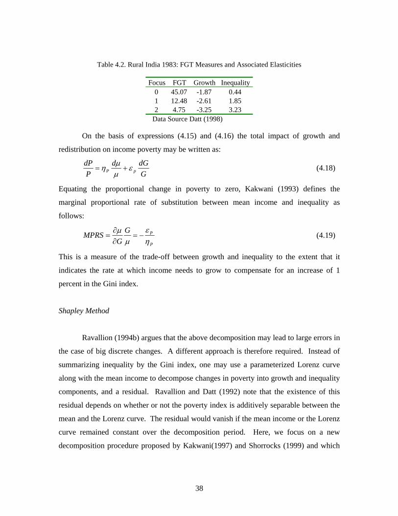
Table 4.2. Rural India 1983: FGT Measures and Associated Elasticities
Focus FGT Growth Inequality0 45.07 -1.87 0.44 1 12.48 -2.61 1.85 2 4.75 -3.25 3.23
Data Source Datt (1998)
On the basis of expressions (4.15) and (4.16) the total impact of growth and
redistribution on income poverty may be written as:
GdGd
PdP
pP εμμη += (4.18)
Equating the proportional change in poverty to zero, Kakwani (1993) defines the
marginal proportional rate of substitution between mean income and inequality as
follows:
P
PGG
MPRSηε
μμ
−=∂∂
= (4.19)
This is a measure of the trade-off between growth and inequality to the extent that it
indicates the rate at which income needs to grow to compensate for an increase of 1
percent in the Gini index.
Shapley Method
Ravallion (1994b) argues that the above decomposition may lead to large errors in
the case of big discrete changes. A different approach is therefore required. Instead of
summarizing inequality by the Gini index, one may use a parameterized Lorenz curve
along with the mean income to decompose changes in poverty into growth and inequality
components, and a residual. Ravallion and Datt (1992) note that the existence of this
residual depends on whether or not the poverty index is additively separable between the
mean and the Lorenz curve. The residual would vanish if the mean income or the Lorenz
curve remained constant over the decomposition period. Here, we focus on a new
decomposition procedure proposed by Kakwani(1997) and Shorrocks (1999) and which
38

does not involve a residual. Shorrocks rationalizes this method on the basis of the
Shapley solution of cooperative games.
The problem of the commons is commonly used to frame the discussion of
cooperative games. A commons is a technology that is jointly owned and operated by a
group of agents. Joint ventures such as law firms, farming or fishing cooperatives are
good examples of commons to the extent that they require coordinated action of partners
with heterogeneous ability. Partners contribute inputs (e.g. labor and or capital) and
share the profit generated by the enterprise (Moulin 2003). The key issue in this context
is how to assess fairly the productive contribution of each partner. The following
definition of the Shapley value is given by Young(1994), in the case of cost sharing.
“Given a cost-sharing game on a fixed set of players, let the players join the cooperative
enterprise one at a time in some predetermined order. As each player joins, the number of players
to be served increases. The player’s cost contribution is his net addition to cost when he joins,
that is, the incremental cost of adding him to the group of players who have already joined. The
Shapley value of a player is his average cost contribution over all possible orderings of the
players.”
To see how the above principle translates into a decomposition procedure,
consider an aggregate statistical indicator such as the overall level of poverty or
inequality. Let it be a function of m contributory factors which together account for the
value of the indicator. The decomposition approach proposed by Shorrocks (1999) is
based on the marginal effect on the value of the indicator of eliminating each of the
contributory factors in sequence. The method then assigns to each factor the average of
its marginal contributions in all possible elimination sequences.
In the case of change in poverty over time, given a fixed poverty line, the level of
poverty at time t is a function of the mean income and the Lorenz curve, P(μt, Lt). The
overall change in poverty from period 1 to period 2 is equal to:
),(),( 1122 LPLPP μμ −=Δ (4.20)
With no change in inequality as measured by the first Lorenz curve, this change in
poverty would be equal to:
39
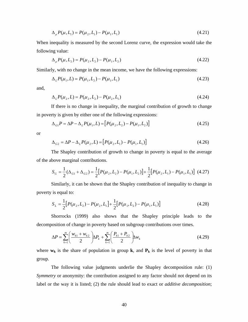
),(),(),( 11121 LPLPLP μμμμ −=Δ (4.21)
When inequality is measured by the second Lorenz curve, the expression would take the
following value:
),(),(),( 21222 LPLPLP μμμμ −=Δ (4.22)
Similarly, with no change in the mean income, we have the following expressions:
),(),(),( 11211 LPLPLPL μμμ −=Δ (4.23)
and,
),(),(),( 12222 LPLPLPL μμμ −=Δ (4.24)
If there is no change in inequality, the marginal contribution of growth to change
in poverty is given by either one of the following expressions:
[ ]),(),(),( 212211 LPLPLPPP LG μμμ −=Δ−Δ=Δ (4.25)
or
[ ]),(),(),( 111222 LPLPLPP LG μμμ −=Δ−Δ=Δ (4.26)
The Shapley contribution of growth to change in poverty is equal to the average
of the above marginal contributions.
[ ] [ ]),(),(21),(),(
21)(
21
1112212221 LPLPLPLPS GGG μμμμ −+−=Δ+Δ= (4.27)
Similarly, it can be shown that the Shapley contribution of inequality to change in
poverty is equal to:
[ ] [ ),(),(21,(),(
21
11211222 LPLPLPLPS L μμμμ −+−= ] (4.28)
Shorrocks (1999) also shows that the Shapley principle leads to the
decomposition of change in poverty based on subgroup contributions over times.
k
m
k
m
k
kkk
kk wPP
Pww
P Δ⎟⎠⎞
⎜⎝⎛ +
+Δ⎟⎠⎞
⎜⎝⎛ +
=Δ ∑ ∑= =1 1
2121
22 (4.29)
where wk is the share of population in group k, and Pk is the level of poverty in that
group.
The following value judgments underlie the Shapley decomposition rule: (1)
Symmetry or anonymity: the contribution assigned to any factor should not depend on its
label or the way it is listed; (2) the rule should lead to exact or additive decomposition;
40
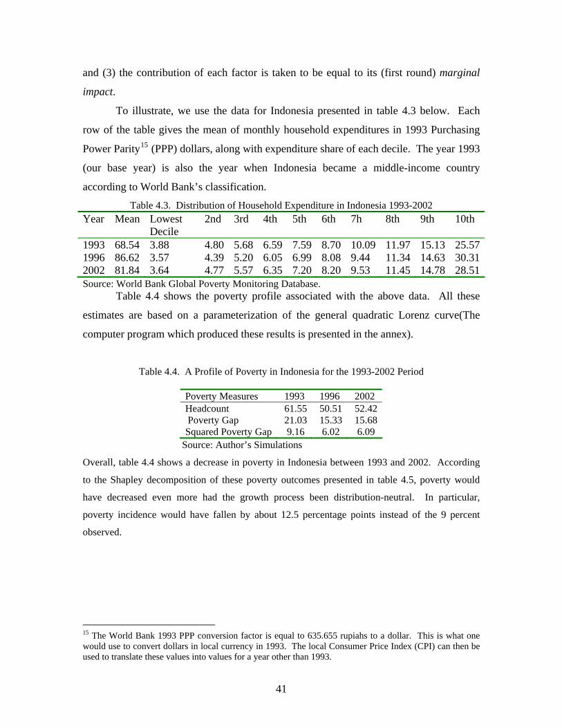
and (3) the contribution of each factor is taken to be equal to its (first round) marginal
impact.
To illustrate, we use the data for Indonesia presented in table 4.3 below. Each
row of the table gives the mean of monthly household expenditures in 1993 Purchasing
Power Parity15 (PPP) dollars, along with expenditure share of each decile. The year 1993
(our base year) is also the year when Indonesia became a middle-income country
according to World Bank’s classification.
Table 4.3. Distribution of Household Expenditure in Indonesia 1993-2002 Year Mean Lowest
Decile 2nd 3rd 4th 5th 6th 7h 8th 9th 10th
1993 68.54 3.88 4.80 5.68 6.59 7.59 8.70 10.09 11.97 15.13 25.571996 86.62 3.57 4.39 5.20 6.05 6.99 8.08 9.44 11.34 14.63 30.312002 81.84 3.64 4.77 5.57 6.35 7.20 8.20 9.53 11.45 14.78 28.51Source: World Bank Global Poverty Monitoring Database. Table 4.4 shows the poverty profile associated with the above data. All these
estimates are based on a parameterization of the general quadratic Lorenz curve(The
computer program which produced these results is presented in the annex).
Table 4.4. A Profile of Poverty in Indonesia for the 1993-2002 Period
Poverty Measures 1993 1996 2002 Headcount 61.55 50.51 52.42 Poverty Gap 21.03 15.33 15.68 Squared Poverty Gap 9.16 6.02 6.09
Source: Author’s Simulations
Overall, table 4.4 shows a decrease in poverty in Indonesia between 1993 and 2002. According
to the Shapley decomposition of these poverty outcomes presented in table 4.5, poverty would
have decreased even more had the growth process been distribution-neutral. In particular,
poverty incidence would have fallen by about 12.5 percentage points instead of the 9 percent
observed.
15 The World Bank 1993 PPP conversion factor is equal to 635.655 rupiahs to a dollar. This is what one would use to convert dollars in local currency in 1993. The local Consumer Price Index (CPI) can then be used to translate these values into values for a year other than 1993.
41

Table 4.5. Shapley Decomposition of Poverty Outcomes in Indonesia, 1993-2002
Measure Total Change Growth Inequality Headcount -9.13 -12.49 3.36 Poverty Gap -5.35 -6.87 1.52 Squared Poverty Gap -3.07 -3.82 0.75
Source: Author’s Simulations
Table 4.6. Shapley Decomposition of Poverty Outcomes in Indonesia, 1996-2002
Measure Total Change Growth Inequality
Headcount 1.91 4.05 -2.14 Poverty Gap 0.35 2.04 -1.69 Squared Poverty Gap 0.07 1.07 -1.00
Source: Author’s Simulations
Focusing on the 1996-2002 sub-period, we note from both table 4.3 and table 4.6
that poverty has increased most likely due to the 1997 Asian crisis. Here again, the
Shapely decomposition reveals that the increase in poverty was less sever because of an
improvement in inequality.
While the above results show a strong link between growth and poverty reduction
in Indonesia between 1993 and 2002, they also reveal the extent to which inequality has
blunted the impacts of both growth and contraction. For a more detailed discussion of
these results see Essama-Nssah (2004).
5. Concluding Remarks
The importance of distributional issues in policymaking creates the need for
empirical tools for assessing the impact of economic shocks and policies on the
distribution of economic welfare. Assuming that individuals are ranked in ascending
order of some welfare indicator, the Lorenz curve transforms the information content of
the cumulative distribution by mapping the cumulative proportion of the population
against the cumulative share of welfare. It also provides an integrative framework for
both the simulation and ethical evaluation of inequality and poverty. The same
framework underlies the assessment of the social impact of economic growth.
42

The structure of the Lorenz curve suggest a simulation strategy for recovering
inequality and poverty measures from information about the mean of the distribution, and
about the slope and its rate of change. The use of numerical integration in simulating
inequality and poverty measures obviates the derivation of special expressions from the
chosen functional form of the Lorenz curve.
Lorenz ranking of distribution respects the Pigou-Dalton principle of transfers
underlying second-order dominance. In the context of pro-poor growth analysis, GIC
dominance [i.e. g(p)≥0 ∀p] respects first-order dominance, while PGC dominance [i.e.
ϕ(p)≥0 ∀p] is consistent with second-order dominance. When dominance tests fail, one
can resort to aggregate indicators for inequality and poverty comparisons. All measures
reviewed here depend to some extent on a focal parameter that can be interpreted as an
indicator of aversion for inequality. This aversion parameter allows the analyst to
calibrate the poverty focus of social impact assessment. Both the extended Gini and the
Atkinson measures can be derived from the concept of equally distributed equivalent
welfare.
Poverty outcomes can be decomposed into growth and inequality components
using either the elasticity approach or the Shapley method. Analysis of data for
Indonesia reveals that absolute and relative indicators of pro-poor growth can lead to
conflicting conclusions from the same set of facts.
43

Annex
A1. Lerman-Yitzhaki Estimator of the Cumulative Distribution Function (CDF)
The Lorenz curve maps the cumulative distribution of the population to the cumulative
distribution of an indicator of economic welfare. It is therefore useful to have a way of estimating
the CDF various situations, particularly when household level data are used to parameterize the
Lorenz curve.
Let x be a welfare indicator assumed to be continuously distributed across a given
population. The cumulative distribution function (CDF) F(x) gives the probability of observing
an individual with a living standard at most equal to x. The slope of this function at a particular
point gives the underlying density function. There are several ways of estimating a cumulative
distribution on the basis of a sample of size n, depending on the method of adjustment for the
non-continuity of the computation. The ordinary approach is to rank the observations in
increasing order of the variable of interest, and divide the rank of each observation by the total
number of observations. Let pr stand for the ordinary estimate of the CDF for observation with
rank r, then we may write:
nrpr = (1)
The density function is linked to the CDF by the relation:
(2) )()()( 1−−= iii xFxFxf
The estimate of the density function associated with (1) is therefore equal to:
n
xf r1)( = (3)
Household level data are usually available in the form of a weighted sample. A
household of a given size represents a certain number of households in the population at large. In
such a case, Lerman and Yitzhaki (1989) recommend the following mid-interval estimator for the
CDF16.
0;2 0
1
0=+= ∑
−
=
ww
wpk
h
khk (4)
16 Deaton (1997:154) proposes a similar procedure for converting household ranks into individual ranks. Assuming that there are whnh people in household h (where nh is the household size and wh its absolute weight), then starting from ρ1=1, the rank of the first person in household h+1 is given by the recursive formula: hhhh wn+=+ ρρ 1 . These ranks can than be normalized relative to the overall population.
44

where wh stands for the relative weight of each individual in household h in the overall
population. This relative weight is equal to the household size times the absolute household
weight divided by total population. Below are a few lines of code fo implementation of the
Lerman-Yitzhaki estimator in EViews.
‘LYCDF.PRG (Progam name) SORT XH ‘Sort in ascending order of xh (per capita welfare indicator) SERIES W1=S*W ‘Inflate Household Size SCALAR TPOP = @SUM(W1) ‘Population SERIES WH=W1/TPOP ‘Relative weight of type h household in the population ‘Compute cumulative distribution F_HAT SMPL @FIRST @FIRST
SERIES FH=WH SMPL @FIRST+1 @LAST FH=FH(-1) + WH
SMPL @ALL SERIES F_HAT = FH – 0.5*WH
A2. Source Code for the Simulation of Inequality and Poverty Measures for Rural India 1983
'INDILORENZ.PRG computes and plots a parameterized Lorenz curve for rural India in 1983 based on data presented in Datt (1998). It then proceedes to computing associate inequality and poverty measures. 'Assumption about form of data available: Income classes with percentage of people and average income in each class. 'EViews 5.1 Standard Edition, January 28, 2005. 'B. Essama-Nssah, PRMPR, The World Bank Group, Washington D.C., January 30, 2005 INCLUDE ATKINSON 'For Atkinson measures INCLUDE ENTROPY 'For generalized entropy measures INCLUDE KAKWANI 'For elasticty of FGT measures INCLUDE LSEGMENT 'Linear Segment Estimator of extended Gini (arguments: cumulative proportion of population and first order derivative of Lorenz function INCLUDE QUADRALORENZ 'General Quadratic Lorenz curve (argument class expenditure shares) ' ----------------------------------- 'DATA PREPARATION MODE QUIET DB INDIRU WFCREATE(WF=RURALINDIA83, PAGE=INITIALDATA) U 13 SCALAR Z=89 'Poverty line in Rupis per capita per month FOR %SR POPSHR AVGX XSHR XWT SERIES {%SR} NEXT
45

POPSHR.LABEL(d) Polulation share POPSHR.LABEL(s) Datt(1998: 2) Table 1; Column 2 POPSHR.LABEL(u) Proportion POPSHR.LABEL(r) Datt Gaurav. 1998. Computational Tools for Poverty Measurement and Analysis. POPSHR.LABEL(r) Food Consumption and Nutrition Division (FCND) Discussion Paper No. 50 POPSHR.LABEL(r) Washington D.C: International Food Policy Research Institute (IFPRI) POPSHR.FILL 0.92, 2.47, 5.11, 7.90, 9.69, 15.24, 13.64, 16.99, 10.00, 9.78, 3.96, 1.81, 2.49 'Percentage POPSHR=POPSHR/100' Proportion AVGX.LABEL(d) Average Monthly per Capita Expenditure AVGX.LABEL(s) Datt(1998: 2) Table 1; Column 3 AVGX.LABEL(u) In Rupis AVGX.LABEL(r) Datt Gaurav. 1998. Computational Tools for Poverty Measurement and Analysis. AVGX.LABEL(r) Food Consumption and Nutrition Division (FCND) Discussion Paper No. 50 AVGX.LABEL(r) Washington D.C: International Food Policy Research Institute (IFPRI) AVGX.FILL 24.84, 35.80, 45.36, 55.10, 64.92, 77.08, 91.75, 110.64, 134.90, 167.76, 215.48, 261.66, 384.97 'Rupis XWT=POPSHR*AVGX SCALAR MUX=@SUM(XWT) XSHR=XWT/MUX '--------------------------------------------------------------- 'PLOT CORRESPONDING LORENZ CURVE SERIES PH 'Cumulative proportion of population SERIES LPH 'Cumulative share of expenditure SMPL @FIRST @FIRST PH=POPSHR LPH=XSHR SMPL @FIRST+1 @LAST PH=PH(-1) + @NAN(POPSHR, 0) LPH=LPH(-1) + @NAN(XSHR,0) SMPL @ALL SERIES L45=PH GROUP LCGRP PH L45 LPH FREEZE(RURALRZ) LCGRP.XY RURALRZ.ADDTEXT(T) Lorenz Curve For Rural India in 1983 RURALRZ.NAME(1) Cumulative Proportion of Population RURALRZ.NAME(2) Line of Complete Equality RURALRZ.NAME(3) Cumulative Proportion of Expenditure '----------------------------------------------------------------------------------------------------------- 'PARAMETERIZE THE LORENZ FUNCTION BASED ON THE GENERAL QUADRATIC MODEL CALL QUADRALORENZ(XSHR) MODEL GQMOD 'General Quadratic Model GQMOD.APPEND LQ=-0.5*(B*PH + E+ @SQRT(M*PH^2 + N*PH+ E^2) )'Lorenz function
46

GQMOD.APPEND FOD=-(B/2)-( (2*M*PH+N)/(4*(@SQRT(M*PH^2+N*PH+E^2)) ))' First Derivative GQMOD.APPEND SOD=((R^2)/8)*1/( (@SQRT( (M*PH^2+N*PH+E^2) ))^3 ) 'Second Derivative STORE A B CC E M N R SA SB MUX Z GQMOD RURALRZ '----------------------------------------------------------------- 'SIMULATE AND PLOT THE LORENZ CURVE PAGECREATE(PAGE=SIMULATION) U 5000 'Choose a wide enough range to make the estimated functions smooth SERIES UNO=1 SERIES PH=@TREND/@OBS(UNO) SERIES L45=PH GROUP LCGRP PH L45 FETCH A B CC E M N R SA SB MUX Z GQMOD 'From INDIRU database GQMOD.SCENARIO ACTUALS GQMOD.SOLVE SMPL @LAST @LAST LQ=1 SMPL @ALL LCGRP.ADD LQ FREEZE(GQLORENZ) LCGRP.XY GQLORENZ.ADDTEXT(T) Simulated Lorenz Curve for Rural India in 1983 GQLORENZ.NAME(1) Cumulative Proportion of Population GQLORENZ.NAME(2) Line of Complete Equality GQLORENZ.NAME(3) Cumulative Proportion of Expenditure '--------------------------------------------------------------------------------------------------------------------- 'COMPUTE EXTENDED GINI COEFFICIENTS USING LOCAL SUBROUTINE LSEGMENT 'DECLARE GLOBAL ARGUMENTS, NUVEC AND GINIVEC, OUTSIDE THE LOCAL SUB ROUTINE VECTOR(6) NUVEC VECTOR(6) GINIVEC CALL LSEGMENT(PH, FOD, NUVEC, GINIVEC) VECTOR GINIVEC=100*GINIVEC 'Scale up to give results in percentage MATRIX(6,4) GINISEN 'The third column will be used later on to store the Sen index of poverty STORE GQLORENZ GINIVEC GINISEN GQMOD '---------------------------------------------------------------------------------------------- 'ESTIMATE LEVEL OF EXPENDITURE AND DENSITY FUNCTION SERIES XP=MUX*FOD SERIES IFX=MUX*SOD SERIES FX=1/IFX SERIES FXDX=0 SMPL @FIRST+1 @LAST FXDX=FX*D(XP) SMPL @ALL '------------------------------------------------------------------- 'COMPUTE MEMBERS OF THE FGT FAMILY VECTOR(3) AVRS 'Aversion for inequality among the poor AVRS.FILL 0,1,2
47

VECTOR(3) FGT SERIES POOR=(XP<=Z) SERIES HEAD=POOR*FXDX FGT(1)=100*@SUM(HEAD) 'Scale up by 100 to get results in percentage SERIES NGAP=(1-XP/Z) 'Poverty gap normalized by poverty line SERIES FGTGAP=POOR*NGAP*FXDX 'Poverty focus of the measure FGT(2)=100*@SUM(FGTGAP) 'Scale up SERIES FGTGPS=POOR*(NGAP^2)*FXDX FGT(3)=100*@SUM(FGTGPS) 'Scale up '-------------------------------------------------------------- 'PLOT THE CORRESPONDING TIP CURVE SMPL @FIRST @FIRST SERIES TIPV =@NAN(FGTGAP, 0) 'Recode NA as Zero (Just in case there are any missing data) SMPL @FIRST+1 @LAST SERIES TIPV=TIPV(-1) + @NAN(FGTGAP, 0) SMPL @ALL SCALAR HDC=FGT(1)/100 SCALAR PVG=FGT(2)/100 SCALAR SPG=FGT(3)/100 GROUP TIPGRP PH TIPV FREEZE(FGTIP) TIPGRP.XY FGTIP.DRAW(DASHLINE, BOTTOM) HDC FGTIP.DRAW(DASHLINE, LEFT) PVG FGTIP.ADDTEXT A TIP Representation of Rural Poverty in India in 1983 '--------------------------------------------------------------------------------------------------------------------- 'COMPUTE ELATICITY WITH RESPECT TO CHANGE IN MEAN CONSUMPTION AND GINI CALL KAKWANI 'Aglobal subroutine 'STORE POVERTY RESULTS IN A TABLE MATRIX(3,4) INDIRUPOV !j=1 FOR %ST AVRS FGT ETAH EPSI COLPLACE(INDIRUPOV, {%ST},!j) !j=!j+1 NEXT FREEZE(POVTAB) INDIRUPOV SETLINE(POVTAB,3) !j=2 FOR %ST FOCUS FGT ETAH EPSI SETCELL(POVTAB, 1, !j, %ST, "C") !j=!j+1 NEXT POVTAB.SETFORMAT(B) G.1 'Show only one significant digit on second column POVTAB.SETFORMAT(R4C3:R6C5) F.2 'Fixed two decimal places from column 3 to column 5 POVTAB.SETTEXTCOLOR(R4C2:R4C5) RED '--------------------------------------------- 'COMPUTE THE WATTS INDEX SERIES WATGAP=(LOG(Z/XP) )*POOR SERIES WATSR=FXDX*WATGAP
48

SCALAR WATTS=@SUM(WATSR)*100 'In percent '-------------------------------------------------------------------------------- 'COMPUTE MEMBERS OF THE CHAKRAVARTY FAMILY 'Chakravarty: CHK when AVRS is 0 or 1 CHK=FGT 'Else SERIES CHKSR= POOR*FXDX*(1 - (XP/Z)^2) SCALAR CHK=@SUM(CHKSR)*100 'In percentage 'Clark, Hemming and Ulph: CHU when AVRS is 0 CHU=WATTS; when AVRS =1, CHU=FGT 'Else SERIES CHUSR=0.5*CHKSR SCALAR CHU=@SUM(CHUSR)*100 'In percentage STORE FGTIP POVTAB WATTS CHK CHU '-------------------------------------------------------- 'COMPUTE GENERALIZED ENTROPY VECTOR(5) AVEC 'Indicator of Aversion VECTOR(5) ENTRO 'Generalized Entropy Measures CALL ENTROPY(FOD, FXDX, AVEC, ENTRO) 'This is a local subroutine with four global arguments ENTRO=100*ENTRO 'In percent '------------------------------------------------------ 'COMPUTE ATKINSON MEASURES 'DECLARE GLOBAL ARGUMENTS OUTSIDE THE LOCAL SUBROUTINE VECTOR(5) ATKIN VECTOR(5) EDEQ CALL ATKINSON(XP, FXDX, ATKIN, EDEQ, MUX) ATKIN=100*ATKIN 'In percent '------------------------------------------------------------------------------------------------------------------- 'BUILD A SINGLE TABLE TO HOLD RESULTS FOR ENTROPY AND ATKINSON MATRIX(5, 4) GENTROPY 'Matrix of inequality indicators !COL=1 FOR %ST AVEC ENTRO ATKIN EDEQ COLPLACE(GENTROPY, {%ST}, !COL) !COL=!COL+1 NEXT FREEZE(ENTROP) GENTROPY SETLINE(ENTROP,3) !CLN=2 FOR %CLB FOCUS ENTROPY ATKINSON EDEX SETCELL(ENTROP, 1, !CLN, %CLB, "C") !CLN=!CLN+1 NEXT ENTROP.SETFORMAT(B) F.1 'Fixed one decimal place on second column ENTROP.SETFORMAT(R4C3:R8C5) F.2 'Fixed two decimal places from column 3 to column 5 STORE ENTROP '------------------------------------------------------ 'COMPUTE SEN INDEX OF POVERTY PAGECOPY(PAGE=SENINDEX, SMPL=@ALL IF POOR) HDC GINISEN GINIVEC XP Z GQMOD DB SEN 'To store objects with same names as content of INDIRU
49

FOR %SR HHSZ HHWT UNO SERIES {%SR}=1 NEXT GROUP RPHH XP HHSZ HHWT 'Representative poor household 'Transform Original Data into Cumulative shares SERIES PCX=RPHH(1)/RPHH(2) 'Total expenditure divided by household size SERIES POPH=RPHH(2)*RPHH(3) 'Population residing in houshold h SERIES WH=POPH/@SUM(POPH)'Population share of household h SERIES PCXW=POPH*PCX 'Population level expenditure in household h SERIES XSHARE=PCXW/@SUM(PCXW) SORT PCX SERIES XPWT=XP*WH SCALAR MUPR=@SUM(XPWT) 'Compute the Cumulative Shares of Population and Corresponding Values of the Lorenz Curve (Use Dynamic Assignment) SMPL @FIRST @FIRST SERIES FHAT=WH SERIES LRNZ =@NAN(XSHARE, 0) 'To protect against missing data, recode NA as zero SMPL @FIRST+1 @LAST SERIES FHAT=FHAT(-1) + WH SERIES LRNZ=LRNZ(-1) + @NAN(XSHARE, 0) SMPL @ALL SERIES PH=FHAT 'Create the 45-Degree Line SERIES L45=PH GROUP LCPR PH L45 LRNZ FREEZE(LCPOOR) LCPR.XY LCPOOR.SCALE(ALL) RANGE(MINMAX) LCPOOR.ADDTEXT(T) Lorenz Curve for Distribution among the Poor LCPOOR.NAME(1) Cumulative Proportion of Population LCPOOR.NAME(2) Line of Complete Equality LCPOOR.NAME(3) Cumulative Proportion of Income 'Parameterize the Lorenz Curve for the Poor COEF(3) BETA SMPL @FIRST @LAST-1 EQUATION GQLC.LS LRNZ*(1-LRNZ)=BETA(1)*(PH^2 - LRNZ) + BETA(2)*LRNZ*(PH - 1) + BETA(3)*(PH - LRNZ) SCALAR A=BETA(1) SCALAR B=BETA(2) SCALAR CC=BETA(3) 'To avoid the reserved name c SCALAR E=-(A+B+CC+1) SCALAR M=(B^2-4*A) SCALAR N=(2*B*E-4*CC) SCALAR R=@SQRT((N^2-4*M*E^2)) SCALAR SA=(R-N)/(2*M) SCALAR SB=-(R+N)/(2*M) SMPL @ALL STORE A B CC E M N R SA SB MUPR Z GQMOD GQMOD.SCENARIO ACTUALS SOLVE GQMOD
50

FOR %VEC GINIPOOR NUV SEN VECTOR(6) {%VEC} NEXT CALL LSEGMENT(PH,FOD,NUV,GINIPOOR) FOR !NU=1 TO 6 SEN(!NU)=100*HDC*(1 - (MUPR/Z)*(1-GINIPOOR(!NU) ) ) 'In percentage NEXT GINIPOOR=100*GINIPOOR 'In percentage '----------------------------------------------------------------------------------- 'LOAD THE GINISEN MATRIX AND FREEZE IT IN A TABLE !J=1 FOR %V NUV GINIVEC GINIPOOR SEN COLPLACE(GINISEN,{%V},!J) !J=!J+1 NEXT FREEZE(GINSENTAB) GINISEN SETLINE(GINSENTAB,3) !CLN=2 FOR %CLB FOCUS GINI GINIPOOR SEN SETCELL(GINSENTAB,1, !CLN, %CLB, "C") !CLN=!CLN+1 NEXT GINSENTAB.SETFORMAT(B) G.1 GINSENTAB.SETFORMAT(R4C3:R9C5) F.2 GINSENTAB.SETTEXTCOLOR(R5C2:R5C5) RED STORE GINSENTAB '-------------------------------------------------------------------------------------- 'CREATE A REPORT PAGE AND BRING IN SOME RESULTS PAGECREATE(PAGE=REPORT) U 1 FETCH GINSENTAB MUPR CLOSE SEN DB INDIRU FETCH CHK CHU ENTROP FGTIP GQLORENZ MUX POVTAB RURALRZ WATTS Z CLOSE INDIRU 'END OF PROGRAM A3.The Subroutines of INDILORENZ.PRG ATKINSON.PRG a local subroutine to compute Atkinson measures of inequality 'B. Essama-Nssah, PRMPR, The World Bank Group, Washington D.C. October 24, 2004 SUBROUTINE LOCAL ATKINSON(SERIES X, SERIES WT, VECTOR ATVEC, VECTOR EDEV, SCALAR MU) 'Set Maximal Level of Aversion and Compute Size of Vector to Hold Results !MAXAV=2 !B=2 !CF=!B-1 !RW=(!B*!MAXAV)+!CF
51

SCALAR ATK 'Atkinson Index of Inequality SCALAR EDE 'Equally Distributed Equivalent Welfare SCALAR SCI 'Social Cost of Inequality SERIES YH=X SERIES YHW=WT*YH SERIES LGYH=LOG(YH) SERIES LGYHW=WT*LGYH !R=1 FOR !EPS=0 TO !MAXAV STEP 1/!B IF !EPS=0 THEN EDE=@SUM(YHW) SCI=MU-EDE ATK=SCI/MU ATVEC(!R)= ATK EDEV(!R)=EDE ELSE IF !EPS=1 THEN EDE=EXP(@SUM(LGYHW)) SCI=MU-EDE ATK=SCI/MU ATVEC(!R)= ATK EDEV(!R)=EDE ELSE SERIES YHWT=WT*(YH)^(1-!EPS) EDE=(@SUM(YHWT))^(1/(1-!EPS)) SCI=MU-EDE ATK=SCI/MU ATVEC(!R)= ATK EDEV(!R)=EDE ENDIF ENDIF !R=!R+1 NEXT ENDSUB ------------------------------------------------------------------------------------------------------------- 'ENTROPY.PRG a subroutine to compute generalized entropy measures of inequality 'B. Essama-Nssah, PRMPR, The World Bank Group, Washington D.C. October 24, 2004 SUBROUTINE LOCAL ENTROPY(SERIES FD, SERIES WT, VECTOR AV, VECTOR GEM) 'Set Maximal Level of Aversion and Compute Size of Vector to Hold Results !MAXAV=2 !B=2 !CF=!B-1 !RW=(!B*!MAXAV)+!CF SCALAR GE SERIES YHMU=FD ' FOD=XP/MUX SERIES INVYM=1/YHMU SERIES LINVYM=LOG(INVYM) SERIES LGYM=LOG(YHMU)
52

!R=1 FOR !THETA=0 TO !MAXAV STEP 1/!B IF !THETA=0 THEN SERIES LINVYMW=WT*LINVYM AV(!R)=!THETA GE=@SUM(LINVYMW) GEM(!R)= GE ELSE IF !THETA=1 THEN SERIES THEILW=WT*(YHMU*LGYM) GE=@SUM(THEILW) AV(!R)=!THETA GEM(!R)=GE ELSE SERIES GETHETA=YHMU^!THETA SERIES GETHETAW=WT*GETHETA AV(!R)=!THETA GE=( @SUM(GETHETAW) - 1)/((!THETA)^2 - !THETA) GEM(!R)=GE ENDIF ENDIF !R=!R+1 NEXT ENDSUB --------------------------------------------------------------------------------------------------------------------- KAKWANI.PRG is a subroutine designed to compute poverty elasticities for the FGT class of poverty measures 'B. Essama-Nssah, PRMPR, The World Bank Group, Washington, D.C. May 28, 2004 SUBROUTINE KAKWANI FOR %V ETAH EPSI MPRS VECTOR(3) {%V} NEXT SCALAR SDPO=((R^2)/8)*1/( (@SQRT( (M*HDC^2+N*HDC+E^2) ))^3 ) SCALAR ETA1=-Z/(MUX*HDC*SDPO) 'Elasticity of Headcount with respect to MU SCALAR ETA2=1-(HDC/PVG) 'Elasticity of Poverty Gap with respect to MU SCALAR ETA3=-2*(PVG-SPG)/SPG 'Elasticity of Square Poverty Gap with respect to MU SCALAR EPSI1=-( (MUX-Z)/Z)*ETA1 'Elasticity of Headcount with respect to Gini SCALAR EPSI2=ETA2+(MUX*HDC)/(Z*PVG) 'Elasticity of Poverty Gap with respect to Gini SCALAR EPSI3=ETA3+(2*MUX*PVG)/(Z*SPG)'Elasticity of Square Poverty Gap with respect to Gini FOR !J=1 to 3 ETAH(!J)=ETA{!J} EPSI(!J)=EPSI{!J}
53

NEXT FOR !J=1 TO 3 MPRS(!J)=-EPSI(!J)/ETAH(!J) 'Marginal proportional rate of substitution between growth and inequality NEXT ENDSUB ------------------------------------------------------------------------------------------------------------ LSEGMENT.PRG is a subroutine designed to compute a vector of extended Gini coefficients based on the Linear Segment Estimator proposed by Chotikapanich and Griffiths 2001. The subroutine requires two series as arguments: P the cummulative proportion of individuals and FOD the first order derivative of the Lorenz function 'B. Essama-Nssah, PRMPR, The World Bank Group. Washington, D.C. October 25, 2004 'EViews 4.1, Standard Edition April 19, 2004 build SUBROUTINE LOCAL LSEGMENT(SERIES P, SERIES FD, VECTOR AVER, VECTOR GINU) SERIES CUMPI=P SERIES QI=(1-CUMPI) SERIES QH=(1-CUMPI(-1)) !AVMAX=6 !B=1 !CF=!B-1 !RWS=(!B*!AVMAX)-!CF !T=1 FOR !NU=1 TO !AVMAX STEP 1/!B SERIES QANU=QI^(!NU) SERIES QBNU=QH^(!NU) SERIES QCNU=QANU-QBNU SERIES QDNU=FD*QCNU SCALAR QDSUM=@SUM(QDNU) GINU(!T)=1+QDSUM AVER(!T)=!NU !T=!T+1 NEXT ENDSUB ------------------------------------------------------------------------------------------------------------ 'QUADRALORENZ.PRG is a subroutine designed to compute parameters of the Lorenz curve based on the General Quadratic model using percentage shares of income or expenditure (when data are organized by income class). 'B.Essama-Nssah, PRMPR, The World Bank Group, Washington D.C. January 29, 2005 'EViews 5.1 SUBROUTINE QUADRALORENZ(SERIES SHR) 'SHR for shares SMPL @FIRST @FIRST SERIES LRNZ =SHR SMPL @FIRST+1 @LAST SERIES LRNZ=LRNZ(-1) + @NAN(SHR, 0) 'Ordinate of the Lorenz curve
54

SMPL @ALL COEF(3) BETA SMPL @FIRST @LAST-1 EQUATION GQLC.LS LRNZ*(1-LRNZ)=BETA(1)*(PH^2 - LRNZ) + BETA(2)*LRNZ*(PH - 1) + BETA(3)*(PH - LRNZ) SCALAR A=BETA(1) SCALAR B=BETA(2) SCALAR CC=BETA(3) 'To avoid the reserved name c SCALAR E=-(A+B+CC+1) SCALAR M=(B^2-4*A) SCALAR N=(2*B*E-4*CC) SCALAR R=@SQRT((N^2-4*M*E^2)) SCALAR SA=(R-N)/(2*M) SCALAR SB=-(R+N)/(2*M) SMPL @ALL ENDSUB A4. Source Code for Pro-Poor Growth Analysis for Indonesia, 1993-2002 INDOPPG.PRG uses parameterized Lorenz curves to implement a pro-poor growth analysis for Indonesia for 1993-1996; 1996-2002. 'EViews 5.1 (Standard Edition January 28, 2005) 'B. Essama-Nssah, PRMPR, the World Bank Group, Washington D.C. February 06, 2005 INCLUDE LSEGMENT INCLUDE QUADRALORENZ INCLUDE PROPOORATE MODE QUIET '--------------------- 'DATA SET UP DB PPG 'For Pro-Poor Growth WFCREATE(WF=INDOPROPOOR, PAGE=POVMODELS) U 11 FOR %SR UNO PH XSHR1 XSHR2 XSHR3 SERIES {%SR} NEXT UNO=1 PH=@TREND/(@OBS(UNO) -1) 'Cumulative proportions of population XSHR1.FILL 0.00, 3.88, 4.80, 5.68, 6.59, 7.59, 8.70, 10.09, 11.97, 15.13, 25.57 'Year 1993 XSHR2.FILL 0.00, 3.57, 4.39, 5.20, 6.05, 6.99, 8.08, 9.44, 11.34, 14.63, 30.31 'Year 1996 XSHR3.FILL 0.00, 3.64, 4.77, 5.57, 6.35, 7.20, 8.20, 9.53, 11.45, 14.78, 28.51 'Year 2002 FOR !S=1 TO 3 XSHR{!S}=XSHR{!S}/100 'To get proportions NEXT
55

VECTOR(3) MUVEC MUVEC.FILL 68.54, 86.62, 81.84 'Mean of monthly household expenditure in 1993 Purchasing Power Parity SCALAR PPP1993=635.655 VECTOR(3) HDCT 'Published poverty incidence HDCT.FILL 0.6155, 0.5051, 0.5242 GROUP SHRGRP XSHR1 XSHR2 XSHR3 '----------------------------------------------- 'PARAMETRIZE LORENZ CURVES FOR !K=1 TO 3 'For 1993 1996 2002 SCALAR MU{!K}=MUVEC(!K) 'Get average monthly expenditure in 1993 PPP dollars from vector MUPP SCALAR HD{!K}=HDCT(!K) CALL QUADRALORENZ(SHRGRP(!K)) 'Estimate the Lorenz functions using the subroutine QUADRALORENZ FOR %ST A B E M N R SA SB RENAME {%ST} {%ST}{!K} STORE {%ST}{!K} MU{!K} 'HDs are the published headcount indices we use to set the poverty lines NEXT MODEL GQMOD{!K} GQMOD{!K}.APPEND LQ{!K}=-0.5*(B{!K}*PH + E{!K}+ @SQRT(M{!K}*PH^2 + N{!K}*PH+ E{!K}^2) )'Lorenz function GQMOD{!K}.APPEND FOD{!K}=-(B{!K}/2)-( (2*M{!K}*PH+N{!K})/(4*(@SQRT(M{!K}*PH^2+N{!K}*PH+E{!K}^2)) ))' First Derivative GQMOD{!K}.APPEND SOD{!K}=((R{!K}^2)/8)*1/( (@SQRT( (M{!K}*PH^2+N{!K}*PH+E{!K}^2) ))^3 ) 'Second Derivative STORE GQMOD{!K} MODEL FGTMOD{!K} FGTMOD{!K}.APPEND HDC{!K}= -( N{!K}+R{!K}*( (B{!K}+(2*PVLN{!K})/MUX{!K})/(@SQRT(((B{!K}+(2*PVLN{!K})/MUX{!K}) )^2 -M{!K} )) ) )/(2*M{!K}) 'Share of Poor in Total Welfare, First and Second Derivatives at headcount, Between Group Inequality FGTMOD{!K}.APPEND LPO{!K}=-0.5*(B{!K}*HDC{!K} + E{!K}+ @SQRT(M{!K}*HDC{!K}^2 + N{!K}*HDC{!K}+ E{!K}^2) ) FGTMOD{!K}.APPEND FDPO{!K} =-(B{!K}/2)-(2*M{!K}*HDC{!K}+N{!K})/(4*@SQRT((M{!K}*HDC{!K}^2+N{!K}*HDC{!K}+E{!K}^2)) ) FGTMOD{!K}.APPEND SDPO{!K}=((R{!K}^2)/8)*1/( (@SQRT( (M{!K}*HDC{!K}^2+N{!K}*HDC{!K}+E{!K}^2) ))^3 ) FGTMOD{!K}.APPEND GBPR{!K}=HDC{!K}-LPO{!K} 'Poverty Gap FGTMOD{!K}.APPEND PVG{!K}=HDC{!K} - (MUX{!K}/PVLN{!K})*( -0.5*( B{!K}*HDC{!K}+E{!K}+ @SQRT( (M{!K}*HDC{!K}^2 + N{!K}*HDC{!K} +E{!K}^2) ) ) ) 'Squared Poverty Gap FGTMOD{!K}.APPEND SPG{!K}= 2*PVG{!K}-HDC{!K}-( (MUX{!K}/PVLN{!K})^2)*(A{!K}*HDC{!K}+B{!K}*( -0.5*( B{!K}*HDC{!K}+E{!K}+@SQRT( (M{!K}*HDC{!K}^2 + N{!K}*HDC{!K} +E{!K}^2) ) ) )-(R{!K}/16)*LOG( (1-HDC{!K}/SA{!K})/(1-HDC{!K}/SB{!K}) ) ) SERIES TRJHDC{!K}=HD{!K} 'Set trejectory Headcount to known values SERIES MUX{!K}=MU{!K}
56

SERIES PVLN{!K} FGTMOD{!K}.CONTROL PVLN{!K} HDC{!K} TRJHDC{!K} SCALAR Z{!K}=PVLN{!K}(1) 'Reinitialize the poverty line to minimize errors associated with parameterization FGTMOD{!K}.SCENARIO ACTUALS FGTMOD{!K}.SOLVE STORE FGTMOD{!K} HD{!K} Z{!K} NEXT '----------------------------------------- 'NEW PAGE FOR SIMULATION PAGECREATE(PAGE=SIMULATION) U 5000 'Choose a wide enough range to make the estimated functions smooth (Lorenz and associated density) VECTOR(3) EMU 'To store estimates of mean expenditure MATRIX(6,4) INDOGINI '---------------------------------------- 'PLOT LORENZ CURVES SERIES UNO=1 SERIES PH=@TREND/@OBS(UNO) SERIES L45=PH VECTOR(6) NUVEC 'Aversion parameters in the extended Gini coefficient FOR !K=1 TO 3 GROUP LCGRP{!K} PH L45 FETCH A{!K} B{!K} E{!K} M{!K} N{!K} R{!K} SA{!K} SB{!K} MU{!K} FGTMOD{!K} GQMOD{!K} HD{!K} Z{!K} GQMOD{!K}.SCENARIO ACTUALS GQMOD{!K}.SOLVE SMPL @LAST @LAST LQ{!K}=1 SMPL @ALL LCGRP{!K}.ADD LQ{!K} FREEZE(LORENZ{!K}) LCGRP{!K}.XY '--------------------------------------------------------------------------------------------------------------------- 'COMPUTE EXTENDED GINI COEFFICIENTS USING LOCAL SUBROUTINE LSEGMENT 'DECLARE GLOBAL ARGUMENTS OUTSIDE THE LOCAL SUBROUTINE VECTOR(6) GINIVEC{!K} CALL LSEGMENT(PH,FOD{!K}, NUVEC, GINIVEC{!K}) '--------------------------------------------------------------------------------------------------------------------- 'ESTIMATE LEVEL AND MEAN OF EXPENDITURE AT PH, AND THE ASSOCIATED DENSITY FUNCTION SERIES MLQ{!K}=MU{!K}*LQ{!K} 'From Generalized Lorenz curve SERIES XP{!K}=MU{!K}*FOD{!K} 'Level of X at PH SERIES IFX{!K}=MU{!K}*SOD{!K} SERIES FX{!K}=1/IFX{!K} 'Density around XP SERIES FXDX{!K}=0 SERIES MUP{!K}=0 SMPL @FIRST+1 @LAST FXDX{!K}=FX{!K}*D(XP{!K}) MUP{!K}=(MLQ{!K})/PH 'Mean at PH SMPL @ALL SERIES EMU{!K}=XP{!K}*FXDX{!K}
57

SCALAR EMUX{!K}=@SUM(EMU{!K}) EMU(!K)=EMUX{!K} NEXT '------------------------------------------------------ 'LOAD EXTENDED GINIS IN MATRIX COLPLACE(INDOGINI,NUVEC, 1) !COL=2 FOR !V=1 TO 3 COLPLACE(INDOGINI,GINIVEC{!V},!COL) !COL=!COL+1 NEXT INDOGINI.SETFORMAT F.2 'Two significant decimals FREEZE(GINITAB) INDOGINI SETLINE(GINITAB,3) !COL=2 FOR %CLB FOCUS GINI93 GINI96 GINI02 SETCELL(GINITAB, 1, !COL, %CLB, "C") !COL=!COL+1 NEXT '----------------------------------------------------------------------------------------------- 'FORMAT GINITAB's COLUMN B CONTAINING AVERSION PARAMETER GINITAB.SETFORMAT(B) G.1 'Show only one digit in this column '-------------------------------------------------------------------- 'CONSTRUCT GROWTH INCIDENCE CURVES PH=100*PH 'Annualized growth rates between 1993 and 2002 SCALAR GAMMA1=(1/9)* ( LOG(MU3) - LOG(MU1)) 'Compute ordinary and relative GIC SERIES GXP13A=100*(GAMMA1 + (1/9)*(LOG(FOD3) - LOG(FOD1) ) ) SERIES GXP13B=100*( (1/9)*(LOG(FOD3) - LOG(FOD1) ) ) GROUP GICS13 PH GXP13A GXP13B FREEZE(GICURVE13) GICS13.XY 'Annualized growth rates between 1996 and 2002 SCALAR GAMMA2=(1/6)* ( LOG(MU3) - LOG(MU2)) 'Compute ordinary and relative GIC SERIES GXP23A=100*(GAMMA2 + (1/6)*(LOG(FOD3) - LOG(FOD2) ) ) SERIES GXP23B=100*( (1/6)*(LOG(FOD3) - LOG(FOD2) ) ) GROUP GICS23 PH GXP23A GXP23B FREEZE(GICURVE23) GICS23.XY 'Store annualized growth rates in a vector VECTOR(2) GRORATES FOR !R=1 TO 2 GRORATES(!R)=100*GAMMA{!R} NEXT '------------------------------------------------------------- 'CONSTRUCT POVERTY GROWTH CURVES SERIES GMUP13 'From 1993 to 2002 SMPL @FIRST+1 @LAST GMUP13=100*(GAMMA1 + (1/9)*(LOG(LQ3) - LOG(LQ1) ) ) SMPL @ALL GROUP PGC13 PH GMUP13
58

FREEZE(PGCURVE13) PGC13.XY SERIES GMUP23 'From 1996 to 2002 SMPL @FIRST+1 @LAST GMUP23=100*(GAMMA2 + (1/6)*(LOG(LQ3) - LOG(LQ2) ) ) SMPL @ALL GROUP PGC23 PH GMUP23 FREEZE(PGCURVE23) PGC23.XY '--------------------------------------------------------------------------------------------------------------------- 'COMPUTE EQUALLY DISTRIBUTED EQUIVALENT GROWTH RATES AND ASSOCIATED DISTRIBUTION ADJUSTMENT FACTORS MATRIX(6,3) THEMAT 'Equally Distributed Equivalent Growth Rates MATRIX(6,3) DAFMAT 'Distribution Adjustment Factors COLPLACE(THEMAT,NUVEC, 1) COLPLACE(DAFMAT,NUVEC, 1) !Q=1 PH=PH/100 'Back to proportions for the following subroutine to work properly FOR %G1 %G2 %W GXP13A GXP13B FXDX1 GXP23A GXP23B FXDX2 {%G1}={%G1}/100 'To make sure the subroutine works properly {%G2}={%G2}/100 CALL PROPOORATE(PH,{%G1},{%W}) 'Note the change in the second argument in order to switch from EDEGR to DAF VECTOR THETA{!Q}=100*THETANU 'Scale up COLPLACE(THEMAT,THETA{!Q},(!Q+1)) CALL PROPOORATE(PH,{%G2},{%W}) VECTOR DAF{!Q}=100*THETANU 'Scale up COLPLACE(DAFMAT,DAF{!Q},(!Q+1)) !Q=!Q+1 NEXT FREEZE(EDERATE) THEMAT FREEZE(DAFTAB) DAFMAT SETLINE(EDERATE,3) SETLINE(DAFTAB,3) !COL=2 FOR %CLB FOCUS PERIOD1 PERIOD2 SETCELL(EDERATE, 1, !COL, %CLB, "C") SETCELL(DAFTAB, 1, !COL, %CLB, "C") !COL=!COL+1 NEXT DAFTAB.SETFORMAT(B) G.1 DAFTAB.SETFORMAT(R4C3:R9C4) F.2 EDERATE.SETFORMAT(B) G.1 EDERATE.SETFORMAT(R4C3:R9C4) F.2 PH=PH*100 'Back to percentages '--------------------------------------------------------------------------------------------- 'COMPUTE MEMBERS OF THE FGT FAMILY AND PLOT TIP CURVES 'Compute Poverty Measures VECTOR(3) ALFA 'ALPHA is a reserved name in EVIEWS 5.1 MATRIX(3,4) INDOPOV ALFA.FILL 0,1,2 FOR !K=1 TO 3 VECTOR(3) FGT{!K}
59

SERIES POOR{!K}=(XP{!K}<=Z{!K}) SERIES HEAD{!K}=POOR{!K}*FXDX{!K} FGT{!K}(1)=100*@SUM(HEAD{!K}) 'Scale up by multipying by 100 SERIES NGAP{!K}=(1-XP{!K}/Z{!K}) SERIES FGTGAP{!K}=POOR{!K}*NGAP{!K}*FXDX{!K} FGT{!K}(2)=100*@SUM(FGTGAP{!K}) 'Scale up SERIES FGTGPS{!K}=POOR{!K}*(NGAP{!K}^2)*FXDX{!K} FGT{!K}(3)=100*@SUM(FGTGPS{!K}) 'Scale up NEXT !COL=1 FOR %ST ALFA FGT1 FGT2 FGT3 COLPLACE(INDOPOV, {%ST}, !COL) !COL=!COL+1 NEXT FREEZE(FGTAB) INDOPOV SETLINE(FGTAB,3) !CLN=2 !ROW=4 FOR %CLB ALFA FGT93 FGT96 FGT02 SETCELL(FGTAB, 1, !CLN, %CLB, "C") !CLN=!CLN+1 NEXT FOR %RLB HDC PVG SPG SETCELL(FGTAB, !ROW, 1, %RLB, "L") !ROW=!ROW+1 NEXT FGTAB.SETFORMAT(B) G.1 FGTAB.SETFORMAT(R4C3:R6C5) F.2 'Construct TIP Curves FOR !K=1 TO 3 SMPL @FIRST @FIRST SERIES TIPV{!K} =100*@NAN(FGTGAP{!K}, 0) 'Recode NA as Zero (Just in case there are any missing data) SMPL @FIRST+1 @LAST SERIES TIPV{!K}=TIPV{!K}(-1) + 100*@NAN(FGTGAP{!K}, 0) SMPL @ALL NEXT GROUP TIPGRP1 PH TIPV1 TIPV3 'TIP for 1993 and 2002 GROUP TIPGRP2 PH TIPV2 TIPV3 'TIP for 1996 and 2002 FOR !j=1 TO 2 FREEZE(FGTIP{!j}) TIPGRP{!j}.XY FGTIP{!j}.DRAW(DASHLINE, BOTTOM) FGT{!j}(1) FGTIP{!j}.DRAW(DASHLINE, LEFT) FGT{!j}(2) NEXT '------------------------------------------------------------------------------------------------------------ 'COMPUTE WATTS INDICES AND ASSOCIATED RATES OF PRO-POOR GRWTH VECTOR(3) WATTS FOR !K=1 TO 3 SERIES LOGZ{!K}=LOG(Z{!K}) SERIES LOGXP{!K}=LOG(XP{!K}) SERIES WATGAP{!K}=FXDX{!K}*(LOG(Z{!K})-LOG(XP{!K}))*POOR{!K}
60

SCALAR WAT{!K}=100*@SUM(WATGAP{!K}) WATTS(!K)=WAT{!K} NEXT WATTS.SETFORMAT F.2 'Mean Growth Rate of the Poor or Rate of Pro-Poor Growth for 1993-2002, and 1996-2002 VECTOR(2) MGRP 'Mean Growth rate of the Poor FOR !T=1 TO 2 SERIES DAF{!T}3WT=(FXDX{!T}*GXP{!T}3B*POOR{!T})/FGT{!T}(!T) SCALAR WDAF{!T}3=@SUM(DAF{!T}3WT) SCALAR GPR{!T}3=100*GAMMA{!T}+WDAF{!T}3 MGRP(!T)=GPR{!T}3 NEXT MGRP.SETFORMAT F.2 '------------------------------------------------------------------------------------------------------------- 'PERFORM SUBPERIOD SHAPLEY DECOMPOSITION OF POVERTY OUTCOMES '**********1993-2002********** FOR !I=1 TO 3 STEP 2 FOR !J=1 TO 3 STEP 2 VECTOR (3) PM{!I}L{!J} NEXT NEXT 'Compute counterfactual poverty indicators members of the Foster-Greer-Thorbecke family based on direct formulae (Datt 1998) FOR !I=1 TO 3 STEP 2 FOR !J=1 TO 3 STEP 2 SCALAR HDC{!I}{!J}= -( N{!J}+R{!J}*( (B{!J}+(2*Z{!I})/MU{!I})/(@SQRT( ( (B{!J}+(2*Z{!I})/MU{!I}) )^2 -M{!J} )) ) )/(2*M{!J}) 'Poverty Incidence SCALAR PVG{!I}{!J}= HDC{!I}{!J} - (MU{!I}/Z{!I})*( -0.5*( B{!J}*HDC{!I}{!J}+E{!J}+ @SQRT( (M{!J}*HDC{!I}{!J}^2 + N{!J}*HDC{!I}{!J} + E{!J}^2) ) ) ) SCALAR SA{!J}=(R{!J} -N{!J})/(2*M{!J}) SCALAR SB{!J}=-(R{!J}+N{!J})/(2*M{!J}) SCALAR SPG{!I}{!J}= 2*PVG{!I}{!J}-HDC{!I}{!J}-( (MU{!I}/Z{!I}) ^2)*(A{!J}*HDC{!I}{!J}+ B{!J}*( -0.5*( B{!J}*HDC{!I}{!J}+E{!J}+@SQRT( (M{!J}*HDC{!I}{!J}^2 + N{!J}*HDC{!I}{!J} +E{!J}^2) ) ) )-(R{!J}/16)*LOG( (1-HDC{!I}{!J}/SA{!J})/(1-HDC{!I}{!J}/SB{!J}) ) ) PM{!I}L{!J}(1)=100*HDC{!I}{!J} 'Scale up PM{!I}L{!J}(2)=100*PVG{!I}{!J} PM{!I}L{!J}(3)=100*SPG{!I}{!J} STORE PM{!I}L{!J} NEXT NEXT MATRIX(3,5) PMLMAT1 !COL=1 FOR %ST ALFA PM1L1 PM1L3 PM3L1 PM3L3 COLPLACE(PMLMAT1, {%ST}, !COL) !COL=!COL+1 NEXT FREEZE(PMLTAB1) PMLMAT1 SETLINE(PMLTAB1,3) !CLN=2
61

!ROW=4 FOR %CLB ALFA PM1L1 PM1L3 PM3L1 PM3L3 SETCELL(PMLTAB1, 1, !CLN, %CLB, "C") !CLN=!CLN+1 NEXT FOR %RLB HDC PVG SPG SETCELL(PMLTAB1, !ROW, 1, %RLB, "L") !ROW=!ROW+1 NEXT 'Compute the Growth and Redistribution Components of Change in Poverty FOR %ST DPOV1 SHAPG1 SHAPD1 VECTOR(3) {%ST} NEXT DPOV1=(PM3L3 - PM1L1) SHAPG1 = 0.5*( (PM3L3 - PM1L3) + (PM3L1 - PM1L1) ) SHAPD1 = 0.5*( (PM3L3 - PM3L1) + (PM1L3 - PM1L1) ) MATRIX (3,3) SHAPMAT1 !COL=1 FOR %ST DPOV1 SHAPG1 SHAPD1 COLPLACE(SHAPMAT1, {%ST}, !COL) !COL=!COL+1 NEXT FREEZE(SHAPTAB1) SHAPMAT1 SETLINE(SHAPTAB1,3) !CLN=2 !ROW=4 FOR %CLB OVERALL GROWTH DISTRIBUTION SETCELL(SHAPTAB1, 1, !CLN, %CLB, "C") !CLN=!CLN+1 NEXT FOR %RLB HDC PVG SPG SETCELL(SHAPTAB1, !ROW, 1, %RLB, "L") !ROW=!ROW+1 NEXT '**********1996-2002********** FOR !I=2 TO 3 FOR !J=2 TO 3 VECTOR (3) PM{!I}L{!J} NEXT NEXT 'Counterfactuals FOR !I=2 TO 3 FOR !J=2 TO 3 SCALAR HDC{!I}{!J}= -( N{!J}+R{!J}*( (B{!J}+(2*Z{!I})/MU{!I})/(@SQRT( ( (B{!J}+(2*Z{!I})/MU{!I}) )^2 -M{!J} )) ) )/(2*M{!J}) 'Poverty Incidence SCALAR PVG{!I}{!J}= HDC{!I}{!J} - (MU{!I}/Z{!I})*( -0.5*( B{!J}*HDC{!I}{!J}+E{!J}+ @SQRT( (M{!J}*HDC{!I}{!J}^2 + N{!J}*HDC{!I}{!J} + E{!J}^2) ) ) ) SCALAR SA{!J}=(R{!J} -N{!J})/(2*M{!J}) SCALAR SB{!J}=-(R{!J}+N{!J})/(2*M{!J}) SCALAR SPG{!I}{!J}= 2*PVG{!I}{!J}-HDC{!I}{!J}-( (MU{!I}/Z{!I}) ^2)*(A{!J}*HDC{!I}{!J}+ B{!J}*( -0.5*( B{!J}*HDC{!I}{!J}+E{!J}+@SQRT(
62

(M{!J}*HDC{!I}{!J}^2 + N{!J}*HDC{!I}{!J} +E{!J}^2) ) ) )-(R{!J}/16)*LOG( (1-HDC{!I}{!J}/SA{!J})/(1-HDC{!I}{!J}/SB{!J}) ) ) PM{!I}L{!J}(1)=100*HDC{!I}{!J} PM{!I}L{!J}(2)=100*PVG{!I}{!J} PM{!I}L{!J}(3)=100*SPG{!I}{!J} STORE PM{!I}L{!J} NEXT NEXT MATRIX(3,5) PMLMAT2 !COL=1 FOR %ST ALFA PM2L2 PM2L3 PM3L2 PM3L3 COLPLACE(PMLMAT2, {%ST}, !COL) !COL=!COL+1 NEXT FREEZE(PMLTAB2) PMLMAT2 SETLINE(PMLTAB2,3) !CLN=2 !ROW=4 FOR %CLB ALFA PM2L2 PM2L3 PM3L2 PM3L3 SETCELL(PMLTAB2, 1, !CLN, %CLB, "C") !CLN=!CLN+1 NEXT FOR %RLB HDC PVG SPG SETCELL(PMLTAB2, !ROW, 1, %RLB, "L") !ROW=!ROW+1 NEXT 'Growth and Redistribution Components FOR %ST DPOV2 SHAPG2 SHAPD2 VECTOR(3) {%ST} NEXT DPOV2=(PM3L3 - PM2L2) SHAPG2 = 0.5*( (PM3L3 - PM2L3) + (PM3L2 - PM2L2) ) SHAPD2 = 0.5*( (PM3L3 - PM3L2) + (PM2L3 - PM2L2) ) MATRIX (3,3) SHAPMAT2 !COL=1 FOR %ST DPOV2 SHAPG2 SHAPD2 COLPLACE(SHAPMAT2, {%ST}, !COL) !COL=!COL+1 NEXT FREEZE(SHAPTAB2) SHAPMAT2 SETLINE(SHAPTAB2,3) !CLN=2 !ROW=4 FOR %CLB OVERALL GROWTH DISTRIBUTION SETCELL(SHAPTAB2, 1, !CLN, %CLB, "C") !CLN=!CLN+1 NEXT FOR %RLB HDC PVG SPG SETCELL(SHAPTAB2, !ROW, 1, %RLB, "L") !ROW=!ROW+1
63

NEXT FOR %TAB1 %TAB2 PMLTAB1 SHAPTAB1 PMLTAB2 SHAPTAB2 {%TAB1}.SETFORMAT(B) G.1 {%TAB1}.SETFORMAT(R4C3:R6C6) F.2 {%TAB2}.SETFORMAT(R4C2:R6C4) F.2 NEXT '--------------------------------------------------------------------------- 'STORE RESULTS AND CHANGE WORKFILE PAGE STORE DAFTAB EDERATE FGTAB FGTIP1 FGTIP2 GINITAB GRORATES LORENZ1 LORENZ2 MGRP PMLTAB1 PMLTAB2 SHAPTAB1 SHAPTAB2 WATTS PAGECREATE(PAGE=REPORT) U 1 FETCH DAFTAB EDERATE FGTAB FGTIP1 FGTIP2 GINITAB GRORATES LORENZ1 LORENZ2 MGRP PMLTAB1 PMLTAB2 SHAPTAB1 SHAPTAB2 WATTS Z1 Z2 Z3 CLOSE PPG 'END OF PROGRAM ------------------------------------------------------------------------------------------------------------ 'PROPOORATE.PRG is a subroutine designed to compute an indicator of the rate of pro-poor growth as a weighted average of points on a Growth Incidence Curve (GIC). The indicator is sensitive to the degree of inequality aversion. 'EViews 4.1, Standard Edition April 19, 2004 build. 'B. Essama-Nssah, PRMPR, The World Bank Group, Washington D.C. May 25, 2004 SUBROUTINE PROPOORATE(SERIES P, SERIES GX, SERIES WHT) 'Percentile, Growth rate of X, Inflation factor SERIES SURVIVE=(1-P) !AVMAX=6 !B=1 !CF=!B-1 !RWS=(!B*!AVMAX)-!CF VECTOR(!rws) NUV 'Indicator of Aversion VECTOR(!rws) THETANU 'Rate of propoor growth !T=1 FOR !NU=1 TO !AVMAX STEP 1/!B SERIES OMEGA=(!NU)*SURVIVE^(!NU-1) SERIES GXWT=GX*WHT SERIES OGXWT=OMEGA*GXWT THETANU(!T)=@SUM(OGXWT) NUV(!T)=!NU !T=!T+1 NEXT ENDSUB
64

References Atkinson, A. B. 1970. On the Measurement of Inequality. Journal of Economic Theory,
2, 244-263. Chotikapanich, Duangkamon and Griffiths, Willianm. 2001. On the Calculation of the of
the Extended Gini Coefficient. Reviwe of Income and Wealth. Series 47, No. 4: 541-547.
Cowell, Frank A. 1995. Measuring Inequality. London: Prentice Hall Chakravarty, S. R. 1983. A New Index of Poverty. Mathematical Social Sciences, Vol.
6. Clark, S.R., Hemming R., Ulph D. 1981. On Indices for Poverty Measurement. Economic Journal. Datt, Gaurav. 1998. Computational Tools for Poverty Measurement and Analysis.
Washington D.C.: International Food Policy Research Institute (IFPRI) Discussion Paper No.50 (Food Consumption and Nutrition Division).
Datt, Gaurav. 1992. Computational Tools for Poverty Measurement and Analysis. Washington D.C.: The World Bank.
Deaton, Angus. 1997. The Analysis of Household Surveys: A Microeconometric Approach to Development Policy. Baltimore: The John Hopkins University Press.
Dixit, Avinash K. 1996. The Making of Economic Policy: A Transaction Cost Politics Perspective. Cambridge, Massachusetts: The MIT Press.
Drazen Allan. 2000. Political Economy in Macroeconomics. Princeton: Princeton University Press.
Essama-Nssah, B. 2004. A Unified Framework for Pro-Poor Growth Analysis. Policy Research Working Paper No. 3397. Washington, D.C.: The World Bank.
_____________. 2002. Assessing the Distributional Impact of Public Policy. Policy Research Working Paper No. 2883. Washington, D.C.: The World Bank.
Fields, Gary S. 2001. Distribution and Development: A New Look at the Developing World. New York: Russell Sage Foundation.
Foster J., Greer, J. and Thorbecke, E. 1984. A Class of Decomposable Poverty Measures. Econometrica, Vol. 52, No.3 , 761-766. (May).
Jenkins, S. and Lambert, Peter J. . 1997. Three ‘I’s of Poverty Curves, with Analysis of UK Poverty Trends. Oxford Economic Papers, 49: 317-327.
Kakwani, Nanak. 2000. Growth an Poverty Reduction: An Empirical Analysis. Asian Development Review, Vol.18, No.2: 74-84.
_____________. 1999. Inequality, Welfare and Poverty: Three Interrelated Phenomena. In Jacques Silber (ed.) “Handbook of Income Inequality Measurement”. Boston: Kluwer Academic Publishers.
_____________. 1997. On Measuring Growth and Inequality Components of Changes in Poverty with Application to Thailand. Discussion Paper No. 97/16. School of Economics: The University of New South Wales.
_____________. 1993. Poverty and Economic Growth with Application to Côte d’Ivoire. Review of Income and Wealth, Series 39, No. 2: 121-139.
Kakwani, Nanak and Pernia, Ernesto M. 2000. What is Pro-Poor Growth? Asian Development Review, Vol.18, No.1: 1-16.
65

Kolenikov, Stanislav and Shorrocks, Anthony. 2003. A Decomposition Analysis of Reginal Poverty in Russia. World Institute for Development Economics Research (WIDER) Discussion Paper No. 2003/74.
Kraay, Aart. 2004. When is Growth Pro-Poor? Cross-Country Evidence. World Bank
Policy Research Working Paper No. 3225. Washington, D.C.: The World Bank.
___________. 2002. Growth is Good for the Poor. Journal of Economic Growth, 7: 195-225.
Lambert, Peter J. 2001. The Distribution and Redistribution of Income. Manchester: Manchester University Press.
_____________. 1993. Evaluating Impact Effect of Tax Reforms. Journal of Economic Surveys, Vol. 7, No.3: 205-242.
Lerman, Robert I. and Yitzhaki, Shlomo. 1989. Improving the Accuracy of Estimates of Gini Coefficients. Journal of Econometrics, 42, 43-47.
Mayshar, Joram and Yitzhaki, Shlomo. 1995. Dalton-Improving Indirect Tax Reform.
The American Economic Review, Vol. 85, No. 4: 793-807.
Moulin, Hervé. 2003. Fair Division and Collective Welfare. Cambridge, Massachusetts: The MIT Press.
Ramadas, K., van der Mensbrugghe and Wodon, Quentin. 2002. SimSIP Poverty: Poverty and Inequality Comparisons Using Group Data. Washington, D.C.: The World Bank (mimeo).
Ravallion, Martin and Chen Shaohua. 2003. Measuring Pro-Poor Growth. Economics Letters, 78: 93-99.
Ravallion, Martin. 1994a. Poverty Comparisons. Chur: Harwood Academic. ______________. 1994b. Decomposing Changes in Poverty Measures: A Comment on
Kakwani. Washington, D.C.: The World Bank (mimeo). Ravallion, Martin and Datt, G. 1992. Growth and Redistribution Components of
Changes in Poverty Measures: A Decomposition with Applications to Brazil and India in the 1980s. Journal of Development Economics 38, 275-295
Ravallion, Martin and Huppi, Monika. 1991. Measuring Changes in Poverty: A Methodological Case Study of Indonesia during an Adjustment Period. The World Bank Economic Review, Vol. 5, No.1: 57-82.
Sen, Amartya. 1999. Development as Freedom. New York: Alfred A. Knopf. ___________. 1997. On Economic Inequality: Expanded Edition with a substantial
Annexe by James E. Foster and Amartya Sen. Oxford: Clarendon Press. ___________. 1989. The Concept of Development. In Hollis Chenery and T.N.
Srinivasan (eds), Handbook of Development Economics, Vol. 1. Amsterdam: Elsevier.
Shorrocks, A. F. 1999. Decomposition Procedures for Distributional Analysis: A Unified Framework Based on the Shapley Value. Mimeo, University of Essex.
_____________. 1983. Ranking Income Distributions. Economica 50, 1-17. Watts, H.M. 1968. An Economic Definition of Poverty. In D.P. Moynihan (Ed), On
Understanding Poverty. New York: Basic Books. World Bank. 2000. World Development Report 2000/2001: Attacking Poverty.
Washington, D.C.: The World Bank.
66

Yitzhaki, Shlomo. 1983. On an Extension of the Gini Index of Inequality. International
Economic Review, Vol. 24, No 3: 617-628.
Young, H. Peyton. 1994. Equity: In Theory and Practice. Princeton: Princeton University Press.
Essama-Nssah: THE_LORENZ_CURVE(December 25, 2004); Current Version(March 24, 2005)
67