power functions of the shewhart control chart - iopscience
TRANSCRIPT

Journal of Physics Conference Series
OPEN ACCESS
Power functions of the Shewhart control chartTo cite this article M B C Khoo 2013 J Phys Conf Ser 423 012008
View the article online for updates and enhancements
You may also likeProduct Quality Monitoring of ShewhartChart Based on Function Integration forManufacturing FactoryDan Tang Mengqing TanLi Yan Jiang etal
-
Performance Evaluation of an EWMA pChart Based on Improved Square RootTransformation to detect Small ShiftProcess VariationArumsari and J N Rifqi
-
Modified SPC for short run test andmeasurement process in multi-stationsC K Koh J F Chin and S Kamaruddin
-
This content was downloaded from IP address 17712920652 on 14122021 at 0153
Power functions of the Shewhart control chart
M B C Khoo
School of Mathematical Sciences Universiti Sains Malaysia 11800 Minden Penang Malaysia
Email mkbcusmmy
Abstract The Shewhart control chart is used to check for a lack of control (a shift in the process) However it is insensitive to small shifts To increase the sensitivity of the Shewhart control chart some actions can be taken These include reducing the width of the control limits increasing the subgroup size to reduce the variance of the sample mean and making use of detection rules to increase the sensitivity of the chart All of these actions will influence the power functions of the Shewhart control chart A probability table showing the probabilities of detecting sustained shifts in the process mean calculated using the formulae have been recommended However the calculations of the probabilities using the formulae are complicated and time consuming In this paper a Monte Carlo simulation using the Statistical Analysis System (SAS) is conducted to compute the necessary probabilities These probabilities are closed to that obtained by using the formulae The Monte Carlo simulation method is recommended as a better way to calculate the probabilities as it provides savings in terms of time and cost Besides the Monte Carlo simulation method also provides a higher flexibility in calculating the probabilities for different combinations of the detection rules The results obtained will assist practitioners in designing and implementing the Shewhart chart effectively
1 Introduction The control charting method for controlling the quality of a process in manufacturing was introduced by Dr Walter A Shewhart in the 1920s According to [1] Shewhart defined the product attributes types of product variations and suggested methods on how to collect plot and analyze data In fact control charts used by quality practitioners from all around the world are based on the process control methods provided by Shewhart
The Shewhart control chart plays an important role in Statistical Process Control (SPC) It is able to detect the occurrence of assignable causes quickly in a process control so that investigations of the process and corrective actions can be made promptly before many defective products are produced [2] The main objective of applying the Shewhart chart is not to detect defective products but to prevent failure so that production of low quality products will not happen This move can help in cost savings as well as helping to produce high quality products
The Shewhart chart is powerful in the detection of large shifts in the process mean Nonetheless it exhibits a lack of sensitivity to detect small shifts Many researches have been made by quality experts to improve the charts sensitivity Decreasing the variance of the sample mean by increasing the subgroup size employing a narrower width of the control limits and applying sensitizing rules such as those by [3] [4] [5] and [6] to the Shewhart chart are some of the popular approaches made to
ScieTech 2013 IOP PublishingJournal of Physics Conference Series 423 (2013) 012008 doi1010881742-65964231012008
Published under licence by IOP Publishing Ltd 1
enhance the performance of the chart All these approaches can influence the power functions of the Shewhart chart A probability table showing the probabilities of detecting sustained shifts in the process mean computed by means of formulae was presented by [7] to serve as guidelines to quality practitioners in constructing the Shewhart chart In this paper we present a Monte Carlo simulation method to obtain similar results This research is motivated by the fact that the Shewhart chart is the most well known control charting tool among practitioners and that an in-depth understanding of the power function of this chart will enable a more efficient use of the chart in process monitoring
This paper is organized as follows The Shewhart control chart is presented in Section 2 In Section 3 the power functions of the Shewhart chart are discussed The probability table of the power functions of the Shewhart X chart is explained in Section 4 In Section 5 performance comparisons are made between the probabilities obtained via formulae and that obtained by means of Monte Carlo simulation Finally conclusions are drawn in Section 6
2 The Shewhart control chart The Shewhart control chart is a graphical plot that helps in the study on how a process changes over time The Shewhart chart consists of three lines that are the lower control limit (LCL) upper control limit (UCL) and center line (CL) The construction of the Shewhart chart is based on statistical principles Typically the UCL is plotted 3 above the CL whereas the LCL is plotted 3 below the CL Here CL represents the mean of the sample data We intend to detect a process that is out-of-control when there are sample points plotting beyond the control limits but when the process is in-control we wish that the probability of detecting a false alarm is as small as possible [8]
Assume that a quality characteristic follows a normal distribution with mean and standard
deviation where both and are known If 1 2 nX X X is a sample of size n then the average of this sample is [9]
1 2 nX X XX
n
(1)
and we know that X is normally distributed with mean and standard deviation Xn
Besides
the probability is 1 that any sample mean will fall between
2Zn
(2a)
and
2Zn
(2b)
Hence if and are known equations (2a) and (2b) can be used as upper and lower control
limits of the Shewhart X chart As mentioned earlier it is customary to replace 2Z by 3 so that the
3 limits are used The process mean is out-of-control if the sample mean falls outside these limits In practice and are usually unknown Consequently these parameters are estimated from a set of in-control Phase-I data These estimates should usually be based on at least 20 to 25 samples
3 Power functions of the Shewhart control chart In statistical quality control an inference on the mean of a population can be summarized as the following hypotheses testing
0 0
1 0
H
H
(3)
The definition of power is given by [9]
ScieTech 2013 IOP PublishingJournal of Physics Conference Series 423 (2013) 012008 doi1010881742-65964231012008
2
0 0
Power 1
reject | is false P H H
(4)
where is the probability of a Type-II error In industries the main goal of using a control chart is to minimize the number of defective products produced prior to the detection of a shift in the process mean [10] Hence it is vital to identify and understand the methods that help to increase the power of a control chart so that a quicker detection of process shifts can be attained
It is found that the subgroup size n is used in the calculation of the control limits and sample standard deviation and for this reason n is one of the factors that has a significant impact on the power of a control chart As n increases the power of a control chart increases The application of detection rules can help to enhance the sensitivity of a control chart in detecting process mean shifts Some of the recent works on detection rules also called runs rules were made by [11] [12] [13] [14] and [15]
[9] and [16] provided an overall Type-I error probability when more detection rules are used The overall Type-I error probability is
1
1 1r
i
i
(5)
where Type-I error probability r = number of detection rules used
i Type-I error probability of the thi rule for 12i r Note that equation (5) assumes that the r detection rules are independent of one another
[7] had estimated the probability of the occurrence of a Type-I error in the first k subgroups by using the following four detection rules given in table 1 The four detection rules considered by [7] are as follows Rule 1 Process is out-of-control when one or more points fall above the +3 control limit Rule 2 Process is out-of-control when 2 of 3 consecutive points fall in the same zone and these points
are between the + 2 and + 3 control limits Rule 3 Process is out-of-control when 4 of 5 consecutive points fall in the same zone and these points
are beyond the +1 control limits Rule 4 Process is out-of-control when 8 consecutive points fall in the same zone either above or
below the CL Using more detection rules will increase the sensitivity of a control chart but it will also inflate the overall Type-I error probability Table 1 The probabilities of a Type-I error for several combinations of detection rules 1 to 4 [7]
Detection rules Number of subgroups
1k 2k 3k 4k 5k 6k 7k 8k 9k 10k 1 0003 0005 0008 0011 0013 0016 0019 0021 0024 0027 1 and 2 0003 0006 0011 0015 0020 0024 0028 0034 0039 0043 1 2 and 3 0003 0006 0011 0016 0025 0032 0040 0050 0060 0060 1 2 3 and 4 0003 0006 0011 0016 0025 0032 0040 0060 0070 0080
4 Probability table for the power functions of a Shewhart X chart In this section the method by means of formulae to compute the probabilities of several combinations of detection rules applied on the Shewhart X chart will be discussed The probability table given by [7] will also be discussed
41 Formulae and probability computation for the power functions The symbols that will be used in the following discussion are defined as follows
ScieTech 2013 IOP PublishingJournal of Physics Conference Series 423 (2013) 012008 doi1010881742-65964231012008
3
k number of subgroups
PDS k = probability of detecting an out-of-control signal within k subgroups
kp probability of detecting an out-of-control signal at the thk subgroup The four detection rules employed by [7] as stated in Section 3 are still considered in the following discussion
411 The use of detection rule 1 Assume that a is the probability that an X sample falls above the + 3 limit
Figure 1 Probabilities of an X sample on the Shewhart chart based on detection rule 1
A general formula for detecting an out-of-control signal within k subgroups is given by [7]
1
2 3 1
1
1
1 1 1 1
1
1 1
k
ii
k
ik
i
k
PDS k p
a a a a a a a a a
a a
a
(6)
Note that the case discussed here is only valid for the one sided control chart (upper sided)
412 The use of detection rules 1 and 2 Assume that a the probability that an X sample falls above the + 3 limit b the probability that an X sample falls between the + 2 and the + 3 limits c the probability that an X sample falls between the CL and the + 2 limit
Figure 2 Probabilities of an X sample on the Shewhart chart based on detection rules 1 and 2
ScieTech 2013 IOP PublishingJournal of Physics Conference Series 423 (2013) 012008 doi1010881742-65964231012008
4
When detection rule 2 is applied at least 2 subgroups are required in the analysis The probability obtained will be similar to that in equation (6) except for cases where 2k or more
For case 2k 2p and 2PDS can be computed using [7]
22 bbacap (7)
and
1 2
2
2
2
PDS p p
a ca ba b
a b b c a
(8)
For case 3k 3p and 3PDS are given by [7]
2 23 2 2p abc b c ac (9)
and
1 2 3
2 2 2
2 2 2
3
2 2
1 2 2
PDS p p p
a b b c a abc b c ac
a b ac ab c b c ac
(10)
From a similar manner kp for k = 4 5 hellip 10 can be obtained using the following equations [7]
2 2 2 34 3 2p abc b c ac (11)
2 2 3 2 3 2 3 45 4 2p ab c b c abc b c ac (12)
2 3 3 3 4 2 4 56 3 3 5 2p ab c b c abc b c ac (13)
2 4 3 4 5 2 5 67 6 5 6 2p ab c b c abc b c ac (14)
3 4 4 4 2 5 3 5 6 2 6 78 10 5 7 4p ab c b c ab c b c abc b c ac (15)
3 5 4 5 2 6 3 6 7 2 7 89 4 4 15 9 8 2p ab c b c ab c b c abc b c ac (16)
3 6 4 6 2 7 3 7 8 2 8 910 11 10 21 10 8 2p ab c b c ab c b c abc b c ac (17)
413 The use of detection rules 1 2 and 3 Assume that a the probability that an X sample above the + 3 limit b the probability that an X sample falls between the + 2 and the + 3 limits c the probability that an X sample falls between the + and the + 2 limits d the probability that an X sample falls between the CL and the + limit
Figure 3 Probabilities of an X sample on the Shewhart chart based on detection rules 1 2 and 3
When detection rule 3 is used at least 4 subgroups are required in the analysis Thus the probabilities obtained are similar to that in the equations given in Section 412 except for cases where 4k or more When k 4 kp can be computed using the equations as follows [7]
ScieTech 2013 IOP PublishingJournal of Physics Conference Series 423 (2013) 012008 doi1010881742-65964231012008
5
2 2 2 2 3 3 2 2 2 2 2 4 34 3 6 3 3 3 3 4 2 4p abc abcd abd ac d acd ac ad b c b cd b d c bc (18)
2 3 2 2 2 3 3 4 2 2 3 2 25
2 2 2 2 3 2 3 3 4
2 2 12 14 16 4 4 12
6 6 4 2 4
p ab cd b cd abc d b c d bc d ac d c d ab d b d abcd
b cd ac d abd b d acd ad
(19)
2 2 3 2 2 2 2 2 2 3 2 3 2 4 2 2 3 3 36
3 2 3 2 3 4 2 4 4 5
9 9 30 20 10 16 4 3 3
20 8 10 5 2 5
p ab cd b cd abc d b c d ac d bc d c d ab d b d
abcd b cd ac d abd b d acd ad
(20)
2 2 2 3 2 2 3 2 2 3 2 4 2 4 2 5 2 2 37
3 3 2 3 2 2 3 3 3 3 3 4 3 2 4 3 4 4
2 4 2 4 5 2 5 5 6
19 18 24 25 15 6 3 24
20 60 28 20 16 4 6 5 30
10 15 6 2 6
P ab c d b c d abc d b c d bc d ac d c d ab cd
b cd abc d b c d ac d bc d c d ab d b d abcd
b cd ac d abd b d acd ad
(21)
The probabilities 8p 9p and 10p are computed using Monte Carlo simulation
414 The use of detection rules 1 2 3 and 4 When detection rule 4 is employed at least 8 subgroups are needed in the analysis Thus the probabilities obtained are similar to that in the equations given in Section 413 except for cases where 8k or more Due to the complexity of the equations [7] confirmed that the computation needs more than 12000 combinations to detect a shift and thus instead of using formulae the Monte Carlo simulation method will be used to calculate the probabilities for 8 9 and 10k
42 Probability tables of the power functions A probability table to show the probability of detecting a sustained shift in the process mean calculated using the formulae has been recommended by [7] The characteristics of the probability table include
Size of the shift 11 sizes of shifts are considered in the probability table They are 042 067 095 125 152 172 196 216 248 275 and 300
Number of subgroups k The number of subgroups displayed in the probability table ranges from 1k to 10k
Subgroup size n The subgroup sizes shown by [7] in the probability table are 1n to 10n 12n 15n and 20n
Detection rules Several combinations of the detection rules have been used to obtain the necessary probabilities
5 Performance comparison From the framework of the probability table and the formulae (see also Sections 411 412 413 and 414) given in [7] computer programs are written in the Statistical Analysis System (SAS) software to compute the probabilities of detecting a sustained shift in the mean within certain number of subgroups following the shift Tables 2 to 9 show the results obtained
From tables 2 to 9 we notice that as the shift size increases the probability of detecting a process mean shift increases
regardless of the values of n and k and the combination of the detection rules being used the probability of detecting a process mean shift within k subgroups increases as k increases
for all n shift sizes and combinations of the detection rules the control chart will become more sensitive if we use more detection rules for any k n and
sizes of shifts
ScieTech 2013 IOP PublishingJournal of Physics Conference Series 423 (2013) 012008 doi1010881742-65964231012008
6
Furthermore if we compare table 2 with table 6 we see that the probabilities in table 6 are generally greater than the corresponding probabilities in table 2 Similar trends are observed if we compare the probabilities in table 3 with table 7 table 4 with table 8 and table 5 with table 9 This means that the power of a control chart increases with an increase in the subgroup size irrespective of the value of k size of the shift and detection rules being used Table 2 Probabilities of detecting a sustained shift in the process mean within k subgroups following a shift for 2n using detection rule 1 only
Shift size 1k 2k 3k 4k 5k 6k 7k 8k 9k 10k
042 0010 0017 0024 0033 0041 0048 0056 0064 0070 0078
067 0022 0041 0058 0078 0096 0116 0132 0150 0165 0186
152 0197 0351 0477 0580 0665 0732 0789 0827 0863 0893
172 0289 0488 0629 0735 0812 0867 0902 0928 0948 0963
300 0893 0988 0999 1000 1000 1000 1000 1000 1000 1000
Table 3 Probabilities of detecting a sustained shift in the process mean within k subgroups following a shift for 2n using detection rules 1 and 2
Shift size 1k 2k 3k 4k 5k 6k 7k 8k 9k 10k
042 0010 0021 0037 0054 0071 0087 0104 0118 0133 0147
067 0022 0054 0097 0142 0184 0219 0251 0289 0320 0354
152 0197 0481 0696 0811 0877 0923 0956 0973 0982 0988
172 0289 0626 0831 0910 0954 0978 0989 0994 0998 0999
300 0893 0998 1000 1000 1000 1000 1000 1000 1000 1000
Table 4 Probabilities of detecting a sustained shift in the process mean within k subgroups following a shift for 2n using detection rules 1 2 and 3
Shift size 1k 2k 3k 4k 5k 6k 7k 8k 9k 10k
042 0010 0021 0037 0064 0112 0143 0171 0196 0227 0260
067 0022 0054 0097 0172 0285 0348 0403 0462 0507 0558
152 0197 0481 0696 0882 0960 0980 0991 0997 0998 0999
172 0289 0626 0831 0951 0991 0997 0999 1000 1000 1000
300 0893 0998 1000 1000 1000 1000 1000 1000 1000 1000
Table 5 Probabilities of detecting a sustained shift in the process mean within k subgroups following a shift for 2n using detection rules 1 2 3 and 4
Shift size 1k 2k 3k 4k 5k 6k 7k 8k 9k 10k
042 0010 0021 0037 0064 0112 0143 0171 0233 0275 0320
067 0022 0054 0097 0172 0285 0348 0403 0541 0593 0643
152 0197 0481 0696 0882 0960 0980 0991 0999 1000 1000
172 0289 0626 0831 0951 0991 0997 0999 1000 1000 1000
300 0893 0998 1000 1000 1000 1000 1000 1000 1000 1000
ScieTech 2013 IOP PublishingJournal of Physics Conference Series 423 (2013) 012008 doi1010881742-65964231012008
7
Table 6 Probabilities of detecting a sustained shift in the process mean within k subgroups following a shift for 10n using detection rule 1 only
Shift size 1k 2k 3k 4k 5k 6k 7k 8k 9k 10k
042 0047 0090 0132 0173 0210 0253 0287 0318 0350 0383
067 0189 0340 0466 0568 0652 0715 0769 0810 0843 0872
152 0967 0999 1000 1000 1000 1000 1000 1000 1000 1000
172 0993 1000 1000 1000 1000 1000 1000 1000 1000 1000
300 1000 1000 1000 1000 1000 1000 1000 1000 1000 1000
Table 7 Probabilities of detecting a sustained shift in the process mean within k subgroups following a shift for 10n using detection rules 1 and 2
Shift size 1k 2k 3k 4k 5k 6k 7k 8k 9k 10k
042 0047 0132 0234 0317 0388 0452 0519 0572 0619 0656
067 0189 0466 0682 0797 0876 0921 0950 0966 0979 0988
152 0967 1000 1000 1000 1000 1000 1000 1000 1000 1000
172 0993 1000 1000 1000 1000 1000 1000 1000 1000 1000
300 1000 1000 1000 1000 1000 1000 1000 1000 1000 1000
Table 8 Probabilities of detecting a sustained shift in the process mean within k subgroups following a shift for 10n using detection rules 1 2 and 3
Shift size 1k 2k 3k 4k 5k 6k 7k 8k 9k 10k
042 0047 0132 0234 0389 0566 0645 0715 0771 0817 0855
067 0189 0466 0682 0868 0957 0979 0990 0995 0998 0999
152 0967 1000 1000 1000 1000 1000 1000 1000 1000 1000
172 0993 1000 1000 1000 1000 1000 1000 1000 1000 1000
300 1000 1000 1000 1000 1000 1000 1000 1000 1000 1000
Table 9 Probabilities of detecting a sustained shift in the process average within k subgroups following a shift for 10n using detection rules 1 2 3 and 4
Shift size 1k 2k 3k 4k 5k 6k 7k 8k 9k 10k
042 0047 0132 0234 0389 0566 0645 0715 0846 0883 0914
067 0189 0466 0682 0868 0957 0979 0990 0999 0999 0999
152 0967 1000 1000 1000 1000 1000 1000 1000 1000 1000
172 0993 1000 1000 1000 1000 1000 1000 1000 1000 1000
300 1000 1000 1000 1000 1000 1000 1000 1000 1000 1000
To compare between Wheelers formulae method [7] and the Monte Carlo simulation method the
percentage of difference is computed Comparisons in terms of percentages are made for each probability table using the following formula
Percentage of difference 100s t
t
(22)
where s probability obtained from Monte Carlo simulation t probability calculated using formula The results obtained are shown in tables 10 to 17 From tables 10 to 17 it is obvious that the probabilities obtained by Monte Carlo simulation are closed to that obtained by means of formulae
ScieTech 2013 IOP PublishingJournal of Physics Conference Series 423 (2013) 012008 doi1010881742-65964231012008
8
The boldfaced entries in tables 10 to 17 denote cases where differences in the probabilities between the two methods exist Note that the differences in the probabilities between the two methods are small Table 10 Percentages of difference in probabilities for subgroup size 2n using detection rule 1 only
Shift size 1k 2k 3k 4k 5k 6k 7k 8k 9k 10k
042 20 5 2 3 1 3 3 1 0 0
067 9 1 2 1 0 1 0 0 1 2
152 1 1 1 1 0 0 0 0 0 0
172 1 0 1 1 0 0 0 0 0 0
300 0 0 0 0 0 0 0 0 0 0
Table 11 Percentages of difference in probabilities for subgroup size 2n using detection rules 1 and 2
Shift size 1k 2k 3k 4k 5k 6k 7k 8k 9k 10k
042 20 2 5 1 1 0 2 4 4 3
067 9 3 5 1 1 0 1 3 3 2
152 1 1 1 0 1 0 0 0 0 0
172 1 1 1 1 0 0 0 0 0 0
300 0 0 0 0 0 0 0 0 0 0
Table 12 Percentages of difference in probabilities for subgroup size 2n using detection rules 1 2 and 3
Shift size 1k 2k 3k 4k 5k 6k 7k 8k 9k 10k
042 20 2 5 2 3 1 1 2 1 0
067 9 3 5 2 0 1 2 2 3 2
152 1 1 1 0 0 0 0 0 0 0
172 1 1 1 0 0 0 0 0 0 0
300 0 0 0 0 0 0 0 0 0 0
Table 13 Percentages of difference in probabilities for subgroup size 2n using detection rules 1 2 3 and 4
Shift size 1k 2k 3k 4k 5k 6k 7k 8k 9k 10k
042 20 2 5 2 3 1 1 7 5 0
067 9 3 5 2 0 1 2 2 1 3
152 1 1 1 0 0 0 0 0 0 0
172 1 1 1 0 0 0 0 0 0 0
196 0 1 0 0 0 0 0 0 0 0
300 0 0 0 0 0 0 0 0 0 0
ScieTech 2013 IOP PublishingJournal of Physics Conference Series 423 (2013) 012008 doi1010881742-65964231012008
9
Table 14 Percentages of difference in probabilities for subgroup size 10n using detection rule 1 only
Shift size 1k 2k 3k 4k 5k 6k 7k 8k 9k 10k
042 0 3 2 2 2 0 0 1 1 0
067 0 1 0 0 0 0 0 0 1 1
152 0 0 0 0 0 0 0 0 0 0
172 0 0 0 0 0 0 0 0 0 0
196 0 0 0 0 0 0 0 0 0 0
Table 15 Percentages of difference in probabilities for subgroup size 10n using detection rules 1 and 2
Shift size 1k 2k 3k 4k 5k 6k 7k 8k 9k 10k
042 0 1 1 1 1 1 1 1 1 1
067 0 1 1 0 1 0 0 0 0 0
152 0 0 0 0 0 0 0 0 0 0
172 0 0 0 0 0 0 0 0 0 0
196 0 0 0 0 0 0 0 0 0 0
Table 16 Percentages of difference in probabilities for subgroup size 10n using detection rules 1 2 and 3
Shift size 1k 2k 3k 4k 5k 6k 7k 8k 9k 10k
042 0 1 1 0 0 1 1 0 0 1
067 0 1 1 0 0 0 0 1 0 0
152 0 0 0 0 0 0 0 0 0 0
172 0 0 0 0 0 0 0 0 0 0
196 0 0 0 0 0 0 0 0 0 0
Table 17 Percentages of difference in probabilities for subgroup size 10n using detection rules 1 2 3 and 4
Shift size 1k 2k 3k 4k 5k 6k 7k 8k 9k 10k
042 0 1 1 0 0 1 1 1 0 0
067 0 1 1 0 0 0 0 0 0 0
152 0 0 0 0 0 0 0 0 0 0
172 0 0 0 0 0 0 0 0 0 0
196 0 0 0 0 0 0 0 0 0 0
6 Conclusions The Shewhart chart is the simplest and most popular process monitoring tool in SPC In view of this tables 2 ndash 17 are provided to help practitioners in a quick and effective design and implementation of the Shewhart chart for a more efficient process monitoring system The approach by means of formulae is extremely complicated where it becomes impossible when detection rule 4 is employed (see Section 414) The results of this study given in tables 2 ndash 17 show that the Monte Carlo simulation method is an easier and quicker way to calculate the probabilities of detecting a sustained shift in the process mean within k subgroups for the various detection rules as compared to the calculation of these probabilities using the formulae proposed by [7] On the contrary the Monte Carlo simulation method is not only simple but it is also accurate and less time consuming Furthermore a
ScieTech 2013 IOP PublishingJournal of Physics Conference Series 423 (2013) 012008 doi1010881742-65964231012008
10
higher flexibility in obtaining the probabilities for different combinations of the detection rules can be achieved by means of the Monte Carlo simulation method Acknowledgement This research is supported by the Universiti Sains Malaysia Fundamental Research Grant Scheme (FRGS) no 203PMATHS6711232
References [1] Berger R W and Hart T 1986 Statistical Process Control A guide for Implementation (Marcel
Dekker Inc) [2] Grant E L and Leavenworth R S 1980 Statistical Quality Control 5th ed (New York McGraw-
Hill Book Company) [3] Lim T J and Cho M 2009 Design of control charts with m-of-m m runs rules Qual Reliab Eng
Int 25(8) 1085-1101 [4] Kim Y B Hong J S and Lie C H 2009 Economic-statistical design of 2-of-2 and 2-of-3 runs rule
scheme Qual Reliab Eng Int 25(2) 215-228 [5] Zarandi M H F Alaeddini A and Turksen I B 2008 A hybrid fuzzy adaptive sampling - run rules
for Shewhart control charts Inf Scien 178(4) 1152-70 [6] Antzoulakos D L and Rakitzis C A 2008 The modified r out of m control chart Commun Stat -
Simul Comput 37(2) 396-408 [7] Wheeler D J 1983 Detecting a shift in process average - tables of the power function for X
charts J Qual Technol 15(4) 155-170 [8] Ryan T P 1989 Statistical Methods for Quality Improvement (New York John Wiley amp Sons) [9] Montgomery D C 2001 Introduction to Statistical Quality Control 4th ed (New York John
Wiley amp Sons) [10] Guldner F J 1986 Statistical Quality Assurance (Delmar Publishers Inc) [11] Low C K Khoo M B C Teoh W L and Wu Z 2012 The revised m-of-k runs rule based on
median run length Commun Stat - Simul Comput 41(8) 1463-77 [12] Antzoulakos D L and Rakitzis C A 2008 The revised m-of-k runs rule Qual Eng 20(1) 175-181
[13] Khoo M B C and Ariffin K N 2006 Two improved runs rules for the Shewhart X control chart Qual Eng 18(2) 173-178
[14] Khoo M B C 2003 Design of runs rules schemes Qual Eng 16(1) 27-43
[15] Klein M 2000 Two alternatives to the Shewhart X control chart J Qual Technol 32(4) 427-431
[16] Duncan A J 1986 Quality Control and Industrial Statistics 5th ed (Homewood IL Richard D Irwin)
ScieTech 2013 IOP PublishingJournal of Physics Conference Series 423 (2013) 012008 doi1010881742-65964231012008
11
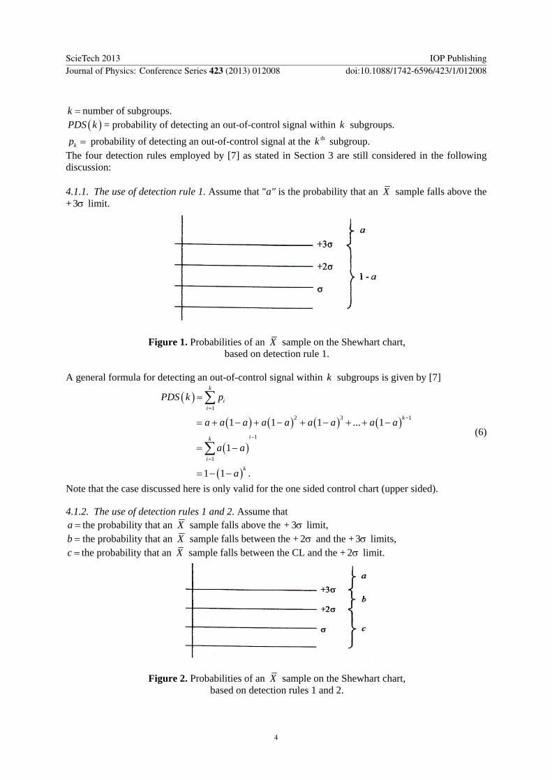