power recycling for an interferometric gravitational wave detector
TRANSCRIPT
THESIS
Power recycling
for an interferometric gravitational wave
detector
Masaki Ando
Department of Physics, Faculty of Science,
University of Tokyo.
December 1998
Contents
1 Introduction 4
2 Gravitational Waves 9
2.1 Wave solutions of the Einstein equation . . . . . . . . . . . . . . . 10
2.1.1 Einstein equation . . . . . . . . . . . . . . . . . . . . . . . 10
2.1.2 Linearized theory . . . . . . . . . . . . . . . . . . . . . . . 10
2.1.3 Gravitational wave . . . . . . . . . . . . . . . . . . . . . . 12
2.1.4 Effect of gravitational waves on free particles . . . . . . . . 13
2.1.5 Polarization . . . . . . . . . . . . . . . . . . . . . . . . . . 14
2.2 Generation of gravitational waves . . . . . . . . . . . . . . . . . . . 15
2.2.1 Radiation of gravitational waves . . . . . . . . . . . . . . . 15
2.2.2 Sources of gravitational waves . . . . . . . . . . . . . . . . 16
2.2.3 Evidence of the existence of a gravitational wave . . . . . 20
2.3 Detection of gravitational waves . . . . . . . . . . . . . . . . . . . 20
2.3.1 Physical and astronomical aims . . . . . . . . . . . . . . . 20
2.3.2 Resonant-mass detectors . . . . . . . . . . . . . . . . . . . 21
2.3.3 Interferometric detector . . . . . . . . . . . . . . . . . . . . 24
2.3.4 Other types of gravitational wave detectors . . . . . . . . . 27
3 Interferometric gravitational wave detector 30
3.1 Michelson interferometer . . . . . . . . . . . . . . . . . . . . . . . 31
3.1.1 Phase detection with a Michelson interferometer . . . . . . 32
3.1.2 Detection of gravitational waves . . . . . . . . . . . . . . . 33
3.1.3 Frequency response and baseline length . . . . . . . . . . 35
3.1.4 Optimization of the frequency response . . . . . . . . . . . 36
0
3.2 Fabry-Perot cavity . . . . . . . . . . . . . . . . . . . . . . . . . . 39
3.2.1 Characteristics of a Fabry-Perot cavity . . . . . . . . . . . 39
3.2.2 Coupling of a cavity . . . . . . . . . . . . . . . . . . . . . 41
3.2.3 FSR and finesse . . . . . . . . . . . . . . . . . . . . . . . . 42
3.2.4 Phase enhancement of a Fabry-Perot cavity . . . . . . . . 43
3.2.5 Response to gravitational waves . . . . . . . . . . . . . . . 45
3.2.6 Storage time . . . . . . . . . . . . . . . . . . . . . . . . . . 46
3.2.7 Response to mirror displacement . . . . . . . . . . . . . . 47
3.2.8 Response to frequency fluctuation . . . . . . . . . . . . . . 48
3.3 Power recycling . . . . . . . . . . . . . . . . . . . . . . . . . . . . 50
3.3.1 Principle of power recycling . . . . . . . . . . . . . . . . . 50
3.3.2 Recycling cavity . . . . . . . . . . . . . . . . . . . . . . . . 51
3.3.3 Power recycling gain . . . . . . . . . . . . . . . . . . . . . 52
3.4 Noise sources for an interferometer . . . . . . . . . . . . . . . . . . 53
3.4.1 Optical readout noise . . . . . . . . . . . . . . . . . . . . . 53
3.4.2 Thermal noise . . . . . . . . . . . . . . . . . . . . . . . . . 56
3.4.3 Seismic noise . . . . . . . . . . . . . . . . . . . . . . . . . . 58
3.4.4 Noises of the laser source . . . . . . . . . . . . . . . . . . 60
3.4.5 Residual gas noise . . . . . . . . . . . . . . . . . . . . . . 62
3.4.6 Noises due to control of the interferometer . . . . . . . . . 63
4 Signal separation scheme 65
4.1 Overview of control schemes . . . . . . . . . . . . . . . . . . . . . 66
4.1.1 Power-recycled Fabry-Perot-Michelson interferometer . . . 66
4.1.2 Frontal modulation . . . . . . . . . . . . . . . . . . . . . 67
4.1.3 Signal separation . . . . . . . . . . . . . . . . . . . . . . . 70
4.2 Frontal modulation . . . . . . . . . . . . . . . . . . . . . . . . . . 71
4.2.1 Modulation and demodulation . . . . . . . . . . . . . . . . 71
4.2.2 Static response of an interferometer . . . . . . . . . . . . . 79
4.2.3 Derivative of the response . . . . . . . . . . . . . . . . . . 81
4.3 Sensitivities of the signals under operational conditions . . . . . . 84
4.3.1 Operational point . . . . . . . . . . . . . . . . . . . . . . . 85
4.3.2 Conditions for the sidebands . . . . . . . . . . . . . . . . . 86
1

4.3.3 Response of the interferometer at the operational point . . 88
4.3.4 Signals extracted using frontal modulation . . . . . . . . . 89
4.4 Signal-separation method . . . . . . . . . . . . . . . . . . . . . . 91
4.4.1 Signal mixing problem . . . . . . . . . . . . . . . . . . . . 92
4.4.2 Sideband elimination . . . . . . . . . . . . . . . . . . . . . 92
4.4.3 Adjustment of the optical parameters . . . . . . . . . . . . 93
4.4.4 Calculation of the signals in a model interferometer . . . . 95
4.4.5 Requirements for signal separation . . . . . . . . . . . . . 96
5 3-m Fabry-Perot-Michelson interferometer 100
5.1 Optical design . . . . . . . . . . . . . . . . . . . . . . . . . . . . . 104
5.1.1 Mirrors . . . . . . . . . . . . . . . . . . . . . . . . . . . . 104
5.1.2 Beam splitter . . . . . . . . . . . . . . . . . . . . . . . . . 106
5.1.3 Pick-off mirror . . . . . . . . . . . . . . . . . . . . . . . . . 107
5.1.4 Fabry-Perot arm cavity . . . . . . . . . . . . . . . . . . . 108
5.1.5 Michelson interferometer and power recycling . . . . . . . . 108
5.2 Suspension system . . . . . . . . . . . . . . . . . . . . . . . . . . . 109
5.2.1 Double pendulum . . . . . . . . . . . . . . . . . . . . . . 109
5.2.2 Isolation ratio . . . . . . . . . . . . . . . . . . . . . . . . 111
5.2.3 Coil-magnet actuator . . . . . . . . . . . . . . . . . . . . 111
5.3 Laser . . . . . . . . . . . . . . . . . . . . . . . . . . . . . . . . . . 113
5.3.1 Laser source . . . . . . . . . . . . . . . . . . . . . . . . . . 115
5.3.2 Mode matching . . . . . . . . . . . . . . . . . . . . . . . . 117
5.3.3 Optical isolators . . . . . . . . . . . . . . . . . . . . . . . . 118
5.4 Signal extraction and control system . . . . . . . . . . . . . . . . . 119
5.4.1 Modulation, demodulation, and control . . . . . . . . . . . 120
5.4.2 Oscillator . . . . . . . . . . . . . . . . . . . . . . . . . . . 121
5.4.3 Phase modulator . . . . . . . . . . . . . . . . . . . . . . . 121
5.4.4 RF photo detector . . . . . . . . . . . . . . . . . . . . . . . 122
5.4.5 Demodulator . . . . . . . . . . . . . . . . . . . . . . . . . 123
5.5 Devices for monitor and measurement . . . . . . . . . . . . . . . . 125
5.5.1 AF photo detector . . . . . . . . . . . . . . . . . . . . . . . 125
5.5.2 Intensity modulator . . . . . . . . . . . . . . . . . . . . . . 125
2

5.5.3 Optical spectrum analyzer . . . . . . . . . . . . . . . . . . 126
5.6 Vacuum system . . . . . . . . . . . . . . . . . . . . . . . . . . . . 126
6 Experiment 128
6.1 Lock acquisition . . . . . . . . . . . . . . . . . . . . . . . . . . . . 129
6.1.1 Correlation diagram . . . . . . . . . . . . . . . . . . . . . . 129
6.1.2 Guide locking scheme . . . . . . . . . . . . . . . . . . . . 131
6.1.3 Automatic locking scheme . . . . . . . . . . . . . . . . . . 135
6.2 Operation with power recycling . . . . . . . . . . . . . . . . . . . 137
6.2.1 Power-recycling gain . . . . . . . . . . . . . . . . . . . . . 138
6.2.2 Stability of operation . . . . . . . . . . . . . . . . . . . . . 139
6.2.3 Control system . . . . . . . . . . . . . . . . . . . . . . . . 142
6.2.4 Calibration of signals . . . . . . . . . . . . . . . . . . . . . 143
6.2.5 Residual RMS deviations . . . . . . . . . . . . . . . . . . 144
6.2.6 Signal gain . . . . . . . . . . . . . . . . . . . . . . . . . . . 145
6.3 Signal separation . . . . . . . . . . . . . . . . . . . . . . . . . . . 147
6.3.1 Mixing in the VRI signal . . . . . . . . . . . . . . . . . . . . 148
6.3.2 Signal sensitivity matrix . . . . . . . . . . . . . . . . . . . 150
6.4 Sensitivity of the interferometer . . . . . . . . . . . . . . . . . . . 151
6.4.1 Displacement noise level . . . . . . . . . . . . . . . . . . . 151
6.4.2 Estimation of noise level . . . . . . . . . . . . . . . . . . . 152
6.4.3 Summary of noise sources . . . . . . . . . . . . . . . . . . 159
7 Discussion and conclusion 163
7.1 Results and discussions . . . . . . . . . . . . . . . . . . . . . . . . 163
7.2 Power recycling in a real detector . . . . . . . . . . . . . . . . . . 165
7.3 Conclusion . . . . . . . . . . . . . . . . . . . . . . . . . . . . . . . 166
References 167
Acknowledgements 174
3
Chapter 1
Introduction
Gravitational waves are ripples of space-time curvature which propagate across
the universe at the speed of light. The existence of gravitational waves has been
predicted as one of the consequences of the General Theory of Relativity [1, 2, 3],
and confirmed as a result of the observation of the binary pulsar PSR 1913+16 [4,
5, 6]. However, gravitational waves have not been directly detected, because of the
weakness of the gravitational interactions. The detection of gravitational waves
will not only confirm the General Theory of Relativity, but also open a new field
of ‘gravitational wave astronomy’. In order to create this new astronomy which
is qualitatively different from that with electro-magnetic waves, several groups
in the world are struggling with development and construction of gravitational
wave detectors.
Mainly, two types of gravitational wave detector have been developed: resonant-
mass type detectors and free-mass type detectors. At first, gravitational waves
were attempted to detect with resonant-mass detectors [7, 8], which are designed
to detect the vibration of an elastic body excited by gravitational waves. Since
many kinds of technology have been developed and accumulated, resonant-mass
detectors have already reached the observation phase. However, a resonant-mass
detector is not suitable for an observation of the waveform of gravitational waves
because it is sensitive only at a narrow frequency range near the resonance of
the elastic body. On the other hand, it is possible to observe the waveform of
gravitational waves with a free-mass detector using a laser interferometer, which
has a wider observation band [9, 10]. Laser interferometric gravitational wave
4

Front mirror
End mirror
Beamsplitter
Laser source Photo detector
Gravitational wave signal
End mirror
Front mirror
Fabry-Perot cavity
Recycling mirror
Figure 1.1: Laser interferometric gravitational wave detector. It is based
on a Michelson interferometer, which detects the differential length change
in two orthogonal optical paths. In practice, a few mirrors are added
to the Michelson interferometer to increase the effective arm length and
laser power. This figure shows a Fabry-Perot-Michelson interferometer with
power recycling, which is mainly discussed in this thesis.
detectors have been energetically developed recently because of their advantages
of a wide observation band and its high potential sensitivity with a larger baseline
length compared with a resonant-mass detectors. At present, four projects are
constructing laser interferometric gravitational wave detectors: the LIGO project
in the United States of America [11], the VIRGO project by Italy and France [12],
the GEO project by Germany and Britain [13], and the TAMA project in Japan
[14].
Gravitational waves are detected with a laser interferometer by measuring
the proper length between mirrors by means of laser light. An interferometric
gravitational wave detector is basically a Michelson interferometer which detects
the differential change in two orthogonal optical path lengths separated by a
beamsplitter (Fig. 1.1). In practice, the interferometer has a little more complex
optical configuration with a few additional mirrors to the Michelson interferom-
eter in order to increase the effective arm length and laser power. In the LIGO,
5

VIRGO, and TAMA detectors, the Michelson interferometer is extended to a
Fabry-Perot-Michelson interferometer with power recycling. On the other hand,
a dual-recycling (signal recycling and power recycling) technique is applied to the
Michelson interferometer in the GEO detector. All of the four projects adopt a
power recycling technique.
Power recycling [15] is a technique to improve the shot-noise limited sensitivity
of an interferometer by enhancing the effective laser power. In order to operate a
Michelson interferometer at its highest sensitivity, the interference fringe must be
dark at the output port of the interferometer. Under this operational condition,
the laser beams reflected by the arm mirrors of the Michelson interferometer
interfere constructively in the direction of the laser source at the beamsplitter;
almost all of the laser power goes back toward the laser source. The recycling
mirror reflects this beam back toward the beam splitter and thus enhances the
laser power in the interferometer, which results in an improvement of the shot-
noise level. Thus, power recycling is indispensable for advanced interferometric
gravitational wave detectors because shot noise is one of the fundamental noise
sources of an interferometer.
Though power recycling will be used in all of the interferometric detectors
under construction, several problems must be solved in order to apply power
recycling to these detectors. One of them is a problem in control of the inter-
ferometer. In order to behave as free masses, the mirrors of an interferometric
gravitational wave detector are suspended as pendulums. Though the suspen-
sion system has another role to isolate the mirror from the seismic motion at the
observation frequency band, the mirror is largely excited by the seismic motion
at the resonant frequency of the pendulum. Thus it is necessary to control the
interferometer in order to keep it at the operational point. However, since a
power-recycled interferometer has a complex and coupled optical configuration,
careful analysis and design are required to extract independent control signals
from the interferometer. In addition, in a power-recycled interferometer, the lock
acquisition is not a simple problem. Since the control signals are linear func-
tions of the motion of the interferometer only around the operational point, it
is not obvious whether the interferometer can be locked at the operational point
from an uncontrolled state. Thus, the controllability and lock-acquisition of a
6

power-recycled interferometer must be tested experimentally.
However, before the research described in this thesis, power recycling has not
been realized nor investigated with an interferometer which has the similar con-
figuration as a real detector: a complex optical configuration with suspended
mirrors. Power recycling has been realized experimentally in several table-top
interferometers with rigidly supported mirrors: a simple Michelson interferome-
ter with power recycling [16], a dual-recycled Michelson interferometer [17], and
power-recycled Fabry-Perot-Michelson interferometers [18, 19, 20, 21, 22, 23].
On the other hand, in interferometers with optical components suspended as
pendulums, power recycling has been realized experimentally only with simple
Michelson interferometers [24, 25, 26]. Thus, it is necessary to realize power
recycling with the same optical configuration as a real interferometric gravita-
tional wave detector: a power-recycled Fabry-Perot-Michelson interferometer or
a dual-recycled Michelson interferometer [27, 28, 29]1.
A prototype interferometer with an arm length of 3 m has been developed at
the University of Tokyo [30, 31]. It has the same characteristics as those of a real
gravitational wave detector; it is a Fabry-Perot-Michelson interferometer with
suspended optical components like LIGO, VIRGO, and TAMA. With this proto-
type interferometer, we have developed the control system for a power-recycled
interferometer. This research contains three topics. The first topic is to realize
power recycling with this prototype interferometer [32]. Since power recycling
was not demonstrated before this research in a suspended Fabry-Perot-Michelson
interferometer, it was quite significant to investigate the lock acquisition process
experimentally. The second topic of this research is to develop a signal-separation
scheme for the control of a power-recycled Fabry-Perot-Michelson interferometer
[33]. In order to operate a power-recycled Fabry-Perot-Michelson interferometer,
four longitudinal degrees of freedom must be controlled to maintain the oper-
ational condition. One of the main problems in controlling a power-recycled
interferometer is that the control signal for the length of the recycling cavity can-
1After power recycling was demonstrated with this research, power recycling was realized
with a 40-m prototype interferometer at California Institute of Technology by the LIGO group
[27] and a 20-m prototype interferometer at National Astronomical Observatory by the TAMA
group [28]. Dual recycling was also realized with a 30-m prototype interferometer at Garching
by the GEO group [29].
7

not be extracted independently with a conventional signal-extraction scheme. To
solve this problem, we have invented a new scheme to separate the signals and
tested it experimentally. The third topic of this research is to estimate the effect
of various noise sources in this prototype interferometer. The role of the control
system is to maintain the stability and, at the same time, the sensitivity of the
interferometer. Thus, the control system of the 3-m prototype interferometer is
designed so as not to degrade the sensitivity of the interferometer.
In this thesis, we describe the results of the power recycling experiments on a
3-m Fabry-Perot-Michelson interferometer with suspended mirrors. In particular,
this thesis is concentrated on the control of the interferometer, which is one of
the main problems in power recycling. In Chapter 2, the physical background
of gravitational waves is described: the propagation, generation, and detection
of gravitational waves. Chapter 3 describes the fundamentals of an interfero-
metric gravitational wave detector: its principle, a Fabry-Perot cavity, the power
recycling technique, and the main noise sources of the detector. In Chapter 4,
we explain the signal-extraction and control scheme for a power-recycled Fabry-
Perot-Michelson interferometer: the conventional scheme, its signal-mixing prob-
lem, and our new signal-separation scheme. The experimental setup of a 3-m
prototype interferometer is given in Chapter 5. Chapter 6 details the experimen-
tal results with power recycling: the lock-acquisition analysis, realization of power
recycling, signal-separation measurements, and noise estimations. In Chapter 7,
we summarize and discuss the achievements and problems with a 3-m prototype
interferometer, and give a prospect for power recycling on real gravitational wave
detectors.
8

Chapter 2
Gravitational Waves
Gravitational waves are ripples of space-time curvature which propagate across
the universe at the speed of light. The existence of gravitational waves was
predicted by A. Einstein as one of the consequences of the General Theory of
Relativity [1, 2, 3]. Gravitational waves are generated by accelerated masses, in
analogy to electro-magnetic waves generated by accelerated charges. The exis-
tence of the gravitational waves has been confirmed indirectly as a result of the
observation of the binary pulsar PSR 1913+16 discovered by R. A. Hulse and
J. H. Taylor [4, 5, 6]. However, gravitational waves have not been directly de-
tected, because of the weakness of the gravitational interactions. The detection
of gravitational waves will not only confirm the General Theory of Relativity, but
also create a new field of a ‘gravitational wave astronomy’.
In this chapter, we review wave solutions of the Einstein equation, generation
of gravitational waves, and its detection.
• Wave solutions of the Einstein equation. The theory of gravitational
waves. Their effect on free particles, and their polarization.
• Generation of gravitational waves. The theory of gravitational radia-
tion. The sources of gravitational waves.
• Detection of gravitational waves. The physical and astronomical aims
of gravitational wave detection. Several types of gravitational wave detec-
tors.
9
2.1 Wave solutions of the Einstein equation
2.1.1 Einstein equation
In the General Theory of Relativity, the four dimensional distance, ds, between
two points in space time, xµ and xµ + dxµ, is given by
ds2 = gµνdxµdxν , (2.1)
where gµν is the metric tensor1. The metric tensor gµν is determined by the
energy-momentum tensor Tµν according to the Einstein equation
Gµν =8πG
c4Tµν (2.2)
Gµν ≡ Rµν − 1
2gµνR, (2.3)
where c and G are the speed of light2 and the gravitational constant3, respectively.
The Christoffel symbol (Γµνλ), the Riemann tensor (Rµ
ναβ), the Ricci tensor
(Rµν), and the Ricci scalar (R) satisfy the following equations:
Γµνλ =
1
2gµα(gαν,λ + gαλ,ν − gνλ,α) (2.4)
Rµναβ = Γµ
νβ,α − Γµνα,β + Γµ
γαΓγνβ − Γµ
γβΓγνα (2.5)
Rµν ≡ Rαµαν (2.6)
R ≡ Rαα. (2.7)
2.1.2 Linearized theory
Though it is difficult to solve the equation analytically, the nature of the gravita-
tional field is investigated by linearizing the equation. In nearly flat space time,
the metric can be treated as a perturbation from the Minkowski metric:
gµν = ηµν + hµν , (2.8)
1Greek indices (α, β, µ, ν, and so on) denote the coordinate numbers from 0 to 3, while
Roman indices (i, j, k, and so on ) denote the coordinate numbers from 1 to 3. The coordinates
are denoted by x0 = ct, x1 = x, x2 = y, and x3 = z. In addition, the indices follow the Einstein
summation convention, i.e. any indices repeated in a product are automatically summed up.2The speed of light: c = 2.99792458 × 10⁸ [m/s].3The gravitational constant: G = 6.67259 × 10⁻¹¹ [N · m2/kg2].
10

where the Minkowski metric ηµν is give by
ηµν =
−1 0 0 0
0 1 0 0
0 0 1 0
0 0 0 1
.
(2.9)
Defining the trace reverse tensor hµν of hµν by
hµν ≡ hµν − 1
2ηµνh (2.10)
h ≡ hαα, (2.11)
and considering only to the first order of hµν , we obtain the equations4
Γµνλ =
1
2(hµ
ν,λ + hµλ,ν − hνλ
,µ) (2.12)
Gµν = −1
2(hµν,α
,α + ηµνhαβ,αβ − hµα,ν
,α − hνα,µ,α). (2.13)
Putting a Lorentz gauge condition
hµν,ν = 0 (2.14)
to Eq. (2.13), we obtain the linearized Einstein equation5
2hµν = −16πG
c4Tµν. (2.15)
4Since |hµν | 1, we can use the relations
hµν = ηµαhαν
hµν = ηναhµα.
.5From Eq. (2.13), we obtain an equation:
Gµν = −122hµν
(2 ≡ − ∂2
c2∂t2+ 4).
11

2.1.3 Gravitational wave
The linearized Einstein equation, Eq. (2.15), in vacuum (Tµν = 0) is
2hµν = 0. (2.16)
Eq. (2.16) has a plane wave solution
hµν = Aµνexp(ikαxα). (2.17)
Under the Lorentz gauge condition, Eq. (2.14), the following equations are satis-
fied:
Aµνkν = 0 (2.18)
kµkµ = 0. (2.19)
Equation (2.18) and (2.19) show that the plane-wave solution Eq. (2.17) is trans-
verse wave which propagates at the speed of light. This plane wave is called a
gravitational wave.
By the gauge transformations called Transverse Traceless gauge (TT gauge)6,
the gravitational waves propergating on the z-direction is written as7
hµν = Aµνeik(ct−z) (2.20)
Aµν =
0 0 0 0
0 h+ h× 0
0 h× −h+ 0
0 0 0 0
,
(2.21)
where k = k0, h+ = Axx, and h× = Axy. This equation means that there are two
independent constants h+ and h×. The angular frequency of the gravitational
waves is written as ω = ck.
6TT gauge condition is described by
Aαα = 0
AµνUν = 0,
where Uν is any constant timelike unit vector.7Uν is selected to be Uν = δν
0.
12

2.1.4 Effect of gravitational waves on free particles
Here we describe the effect of gravitational waves on a free particle. A free particle
obeys the geodesic equation
d
dτUµ + Γµ
αβUαUβ = 0, (2.22)
where Uµ is the four velocity of the particle, and τ is the proper time. We
consider the motion of this particle in a background Minkowski space time where
the particle is initially at rest, under the TT gauge condition. The initial condition
for Uµ is
(Uµ)0 = (1, 0, 0, 0) (2.23)
Substituting Eqs. (2.12) and (2.23) to Eq. (2.22), and considering that hα0 = 0
(here we consider the gravitational waves described by Eqs. (2.20) and (2.21)),
the initial four accelerations of the particle is(dUµ
dτ
)0
= −Γµ00 = −1
2ηµα(hα0,0 + h0α,0 − h00,α)
= 0. (2.24)
This equation shows that the particle initially at rest does not change its position
in the TT gauge. In order to see the effect of gravitational waves, consider
the proper length between nearby particles (P1 and P2) which have the position
(0, 0, 0) and (ε, 0, 0) (|ε| 1) in the TT gauge, respectively. When gravitational
waves described by Eqs. (2.20) and (2.21) incident on these particles, the proper
distance between P1 and P2 changes as∫ P2
P1
|gµνdxµdxν| 12 =
∫ ε
0
|gxx|12 dx ' |gxx(P1)|
12 ε
'[1 +
1
2hxx(P1)
]ε. (2.25)
This equation show that the gravitational wave changes the proper distance be-
tween two free particles. Thus, gravitational waves can be detected by monitoring
the distance between free particles.
13
mode
mode
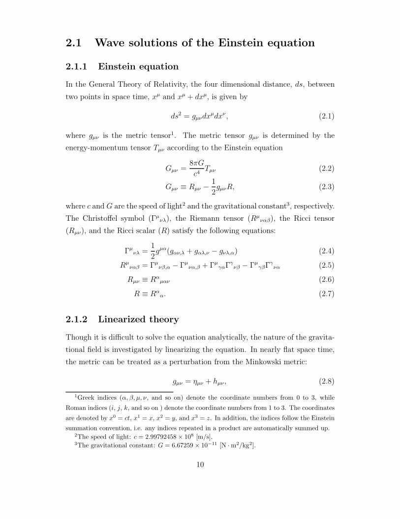
Figure 2.1: Distortions of a circle of free particles caused by gravitational
waves incident from the perpendicular direction of this paper. The upper
and lower figures show the distortions by +mode waves and ×mode waves,
respectively.
2.1.5 Polarization
In order to investigate the effect of gravitational waves on free particles, we con-
sider the case that the particles P1 and P2 are separated by an infinitesimal vector
ξi.
From Eq. (2.22), the equation of geodesic deviation is described
d2
dτ 2ξi = Ri
αβjUαUβξj (2.26)
Taking to the first order of hµν under consideration8, Eq. (2.26) is written as
1
c2
∂2
∂t2ξi = −Ri
0j0ξj. (2.27)
8In this approximation,
Uα ' (1, 0, 0, 0)
τ ' ct.
14

In addition, since
Ri0j0 = − 1
2c2
∂2hij
∂t2
is satisfied under the TT gauge condition, Eq. (2.27) is written as
∂2
∂t2ξi =
1
2
∂2hij
∂t2ξj . (2.28)
Solving this equation so as not to get infinity in t → ∞, we obtain
δξi =1
2hi
jξj , (2.29)
where δξi is the deviation of ξi.
When gravitational waves propagating in the z-direction incident on these
particles, hµν is represented by Eqs. (2.20) and (2.21). Thus, we obtain(δξx
δξy
)=
1
2h+
(ξx
−ξy
)eik(ct−z) +
1
2h×
(ξy
ξx
)eik(ct−z). (2.30)
In Eq. (2.30), the first and second terms represents the two polarizations of grav-
itational waves (+ mode and × mode, respectively). The names of the polariza-
tions correspond to the shape of the deviations of the particles initially arranged
in circle in x-y plane (Fig. 2.1).
2.2 Generation of gravitational waves
2.2.1 Radiation of gravitational waves
The radiation of gravitational waves is explained in an analogy of the radiation
of electro-magnetic waves. Gravitational waves are radiated from accelerated
masses as electro-magnetic waves are radiated from accelerated charges. While
the dominant contribution to the electro-magnetic-wave radiation comes from the
time variation of the electric dipole moment, the gravitational dipole radiation
are forbidden by the conservation laws of momentum and angular momentum.
In a typical case that the motion within the source is slow enough compared
with the speed of light (a slow-motion approximation), the gravitational wave
radiation is contributed by the time variation of the gravitational quadrupole
15

moment. To describe the gravitational wave, we use a reduced quadrupole mo-
ment defined by
I-(t) =
∫ρ(t,x)
(xixj − 1
3δijx
ixj
)d3x, (2.31)
where ρ(t,x) is a mass density. The radiated gravitational wave is written using
the second derivative of I-ij(t) with respect to the time:
hij(t) =2G
c4rI-(t− r
c), (2.32)
where r is the distance from the observation point to the source. From the above
equation, the gravitational wave propagating along the z-direction is written as
h+(t) =2G
c4r
I-11(t− rc) − I-22(t− r
c)
2
h×(t) = −2G
c4rI-12(t− r
c),
The luminosity of the gravitational waves (the averaged energy flux) is written
as
LGW =G
5c5
⟨∑ij
...I-
2ij
⟩. (2.33)
2.2.2 Sources of gravitational waves
If gravitational waves could be generated artificially, it would be possible to test
their existence and to study their nature. However, it is quite difficult to generate
gravitational waves strong enough for laboratory experiments9. Thus, the exper-
imental studies of gravitational waves is directed toward the natural sources, in
particular toward the astronomical sources.
Here we estimate roughly the amplitude of gravitational waves from astro-
nomical sources. Writing I-ij by a corresponding mass energy10, I-ij = Mqc2, the
9As an example, we consider gravitational waves from a rotating dumbbell (two massive
balls connected with a bar). The radiated energy is LGW ∼ 10−27 erg/s (10−34 W), when the
weight of the masses is 100 kg, length of the bar is 2 m, and the rotation frequency is 100 Hz.
The amplitude of the gravitational wave from this dumbbell is hij . 10−43 [34].10The second derivative of a quadrupole momentum I-ij has a dimension of energy:
I-ij ∼ (mass in motion) × (system size)2
(system transit time)2∼ (quadrapole kinetic energy).
16
amplitude of the radiated gravitational wave is described from Eq. (2.32) as
hij ∼ 5 × 10⁻²¹
(Mq
M
)(20 Mpc
r
), (2.34)
where M is the mass of the sun. The value r ∼ 20 Mpc is the distance to the
Virgo cluster. A few bursts of gravitational waves at high frequency (less than a
few kilohertz) are expected in a year among the galaxies included within a 20 Mpc
sphere, which could be detected with ground-based detectors.
Expected main gravitational wave sources [3, 34, 35, 36] are described below.
Here the sources are classified by the waveform: burst waves, periodic waves, and
stochastic waves.
Burst sources
Bursts of gravitational waves are generated by supernova explosions, coalescence
of compact binaries, stars falling into super massive black holes, and so on.
One type of supernova explosions is triggered by the collapse of a stellar
core to a neutron star, when the star has exhausted its supply of nuclear fuel.
Gravitational waves are expected to be generated in the explosion and in the
instability after the explosion. Supernova events are estimated to occur a few
times per century in our galaxy (h ∼ 10−18), and a few times per year within
20 Mpc distance (h ∼ 10−21). The frequency of the radiated gravitational waves is
expected to be below a few kilohertz. Burst gravitational waves are also radiated
in star collapses to black holes. The event rate is not well known; the upper limit
for the collapse-formation of super massive black holes is a few per year in 3 Gpc.
The other reliable gravitational wave sources are coalescing compact binaries
composed of compact stars as neutron stars (NSs) and black holes (BHs). A bi-
nary system loses its orbital energy, radiating periodic gravitational waves. Then,
at last, the compact objects collide and coalesce, radiating a strong quasi-periodic
gravitational waves in a few minutes. The gravitational waves from a coalescence
binary have the waveform of ‘chirp’; both frequency and amplitude increase with
time. The event rate of coalescence of neutron star binaries is estimated to be
about a few times per year within 200 Mpc. In the last 15 minutes, the waves
from coalescing NS-NS binaries will have frequencies from about 10 Hz up to a
few kHz, and will radiate gravitational waves with an amplitude of h ∼ 10−21.
17
Strong gravitational waves will be also radiated from coalescence of massive black
hole (MBH) binaries. Their event rate is estimated to be once per year within
a distance of 3 Gpc. Gravitational waves from a MBH-MBH binary at this dis-
tance will have a chirp waveform sweeping upward from h ∼ 10−20 at 10−4 Hz to
h ∼ 10−18 at 10−2 Hz in the final year of coalescence for MBHs with a mass of
105M.
Burst waves are also radiated from stars spiraling into MBHs thought to
inhabit galactic nuclei. The frequency of the radiated waves is around 10−3 Hz
for a MBH of 107M; the waveform is strongly influenced by the spin of the
MBH. The amplitude would be h ∼ 10−22 for a 1M star spiraling into MBH
at a distance of 20 Mpc. Though the event rate is not well known, it will be
reasonable in a 20 Mpc range, which contains ∼100 galaxies.
Periodic sources
Periodic gravitational waves are radiated from binary stars and from rotating
neutron stars (pulsars).
Binary star systems are certain sources of continuous gravitational waves;
the waveform is computed with confidence from the measured mass and orbital
parameters. In addition, gravitational waves from a neutron star binary have
been observed indirectly (described in the following Section). In order to radi-
ate strong periodic gravitational waves, the binary systems must be comprised
of compact stars: white dwarfs (WD), neutron stars, or black holes. WD-WD
binaries are thought to be so numerous in our galaxy that they will not resolv-
able. They are considered to form a stochastic background with an amplitude of
h ∼ 10−21 around 10−3 Hz. However, there thought to be a large number of re-
solvable sources with higher frequency or larger amplitude than the background.
Considering a NS-NS binary in our galaxy (∼ 10 kpc), gravitational waves with
h ' 4 × 10⁻²² will be radiated at a frequency of 5 × 10⁻³ Hz. The effective
amplitude of these waves is 2 × 10⁻¹⁹ with one year of integration time.
When a single rotating neutron star deviates from axisymmetry about its
principle axis, it will radiate gravitational waves at twice its rotation frequency,
and at the beat frequency of the rotation and precessional frequencies. The am-
plitude is estimated to be h ∼ 10−25 for a pulsar at 1 kpc distance with a rotation
18

frequency of 200 Hz and an ellipticity of 10−6 in the equatorial plane. Though
the amplitude is rather small, the signal can be enhanced with a long integration
time because the rotation frequency is precisely known by the electromagnetic
observation of the pulsar. The effective signal is enhanced by the square root
of the number of cycles, by a factor of 104 in a one week observation period for
200 Hz waves.
Stochastic sources
Besides the background caused by the dense galactic binary systems, a stochastic
background of gravitational waves is expected to be produced in the big bang, in
phase transitions in the early universe, and from cosmic strings.
One of the predicted origins of the stochastic background of gravitational
waves is the big bang itself; these background waves are called primordial gravita-
tional waves. It is estimated that that the gravitational waves have not interacted
with matter since the Planck era, when space and time came into being, and that
primordial gravitational waves should not have been thermalized by interactions
with matter. On the other hand, the gravitational waves emerged from the big
bang are considered to have interacted with the subsequent, early-time expansion
of the universe to produce a stochastic background today.
The cosmological gravitational wave background is often discussed in terms
of Ωg(f), the energy density per logarithmic frequency interval relative to the
closure density (the critical energy density necessary to close the universe). The
RMS amplitude of the fluctuating gravitational waves in a bandwidth of f at a
frequency of f is expressed by Ωg in the relation h ∼ 1 × 10⁻¹⁸√
Ωg (1 Hz/f) ,
assuming a Hubble constant of 75 km · s−1 · Mpc−1. The observation of the cosmic
microwave radiation sets a limit of Ωg ≤ 10−9 at 10−18 Hz.
A stochastic background could also have been produced by phase transitions
associated with QCD interactions and with electroweak interactions during the
early expansion of the universe. If the collision of vacuum bubbles have occurred
in the electroweak phase transition, the gravitational wave background might
have a density of Ωg ∼ 3 × 10⁻⁷ around 0.1 mHz.
It is suggested that cosmic strings have been created in a phase transition as-
sociated with the grand-unified interactions long before the QCD and electroweak
19

phase transitions. The vibrations of the cosmic strings would produce gravita-
tional waves with almost a flat spectrum of Ωg independent of the frequency. The
suggested waves have a strength of Ωg ∼ 10−7, which is already constrained by
pulsar timing observations.
2.2.3 Evidence of the existence of a gravitational wave
The existence of a gravitational wave has been confirmed by the observation of a
binary pulsar. In 1974 the binary pulsar PSR 1913+16 was found by R. A. Hulse
and J. H. Taylor [4]. From the observed parameters of this system, including
orbital precession, gravitational red shift, and radiation time delay, nearly all of
the relevant properties of this binary system are determined. In particular, the
masses of the pulsar and the companion star have been determined in a very good
precision11.
PSR 1913+16 shows the self-consistency of the General Theory of Relativity
in a very good precision. One of the most important results from the observation
of this binary system is the change in the orbital period due to the radiation
of gravitational waves [5, 6]. The binary system radiates gravitational waves in
the radiation rate described in Eq. (2.33). Since the orbital energy is carried
away by the gravitational wave radiation, the orbital period of the binary system
decreases. The observed change in the orbital period agrees with that predicted
by the General Theory of Relativity within the experimental accuracy, better
than one per cent.
2.3 Detection of gravitational waves
2.3.1 Physical and astronomical aims
The existence of gravitational waves has been predicted theoretically, and con-
firmed by the observation of a neutron-star binary. However, gravitational waves
have not been detected directly, because of the weakness of gravitational inter-
actions. The detection of gravitational waves is one of the most important tasks
11The 1993 Nobel Prize in Physics was awarded to R. A. Hulse and J. H. Taylor for their
discovery of the binary pulsar and indirect observation of a gravitational wave.
20
left for us in order to verify the General Theory of Relativity. In addition, the de-
tection of gravitational waves has a possibility to open a new observation window
to the universe. The information obtained from the waveform of gravitational
waves is different in quality from that of electro-magnetic waves: since gravi-
tational waves transmits almost everything, they inform us about the dynamic
motion of astronomical objects. It is expected that the waveform of gravitational
waves might give us information such as: the Hubble constant, the state equation
of a neutron star, the mechanism of supernova explosions, understandings of the
strong gravitational field, and information about the early universe.
The attempt to detect gravitational waves is pioneered by J. Weber [7, 8]. He
used resonant-type detectors, which detect the vibration of massive metal bars
excited by gravitational waves at their resonant frequency. Currently, laser inter-
ferometric detectors [9] are investigated and constructed vigorously. An interfer-
ometric detector measures the distance between free-falling masses perturbed by
gravitational waves. One of the advantages of an interferometric detector is its
broad observation band, which enables us to observe the waveform of gravitational
waves. While resonant-type detectors and interferometric detectors on the ground
aim at high frequency (10 Hz ∼ 1 kHz) gravitational waves, lower frequency
gravitational waves are tried to detect by a Doppler tracking method, a space
interferometer (10−4 ∼ 10−1 Hz), and a pulsar timing method (10−9 ∼ 10−7 Hz).
At extremely low frequencies (10−18 ∼ 10−15 Hz), the gravitational waves would
be measured as quadrupolar anisotropies in the cosmic microwave background.
2.3.2 Resonant-mass detectors
Principle of a resonant-type detector
A resonant-type detector is comprised of a massive elastic body (an antenna) and
a vibration detector (a transducer) [7]. A part of the energy of incident gravita-
tional waves is converted to vibration energy of the elastic body. A transducer
detects the vibration as a gravitational wave signal.
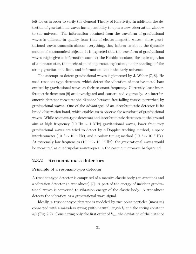
Ideally, a resonant-type detector is modeled by two point particles (mass m)
connected with a mass-less spring (with natural length l0 and the spring constant
ks) (Fig. 2.2). Considering only the first order of hµν , the deviation of the distance
21

spring
mass
Gravitational wave signal
Transducer
Figure 2.2: Resonant-type gravitational waves detector, modeled by two
masses connected with a spring. Gravitational waves excite the oscillator,
which is detected with a transducer.
of two particles δξµ is written as
∂2δξi
∂t2+
ω0
Q
∂δξi
∂t+ ω0
2δξi =1
2
∂2hij
∂t2ξj , (2.35)
where Q is the quality factor (Q-value) of the resonance, and ω0 =√
ks/m is the
resonant angular frequency of this system. Equation (2.35) represents a damped
harmonic oscillator excited by a gravitational wave force12. When the frequency
of the incident gravitational waves is near the resonant frequency of the detector,
the vibration is excited efficiently.
The energy which the detector receives from the incident gravitational waves
is proportional to the mass of the antenna, and to the square of the Q-value and
l0. Thus, the antenna is made of a few tons of metal with small losses (usually,
aluminum or Niobium is used). The sensitivity is mainly limited by the thermal
motion of the elastic body, and the readout noise of the transducer. In order to
reduce the effect of the thermal noise, the detector is usually operated at cryogenic
temperatures. In addition, low-noise transducers have been developed.
Development of resonant-mass detectors
Table 2.1 shows the operated and planned resonant-type detectors. The develop-
ment of resonant-mass gravitational wave detectors is pioneered by J. Weber [7],
and the sensitivities have been improved by a number of other research groups
since then. Weber’s detector consisted of two sets of bar-type resonant detectors
12In the limitation of ω0 → 0 and Q → ∞, the equation reduces to the deviation of free
particles, Eq. (2.28).
22
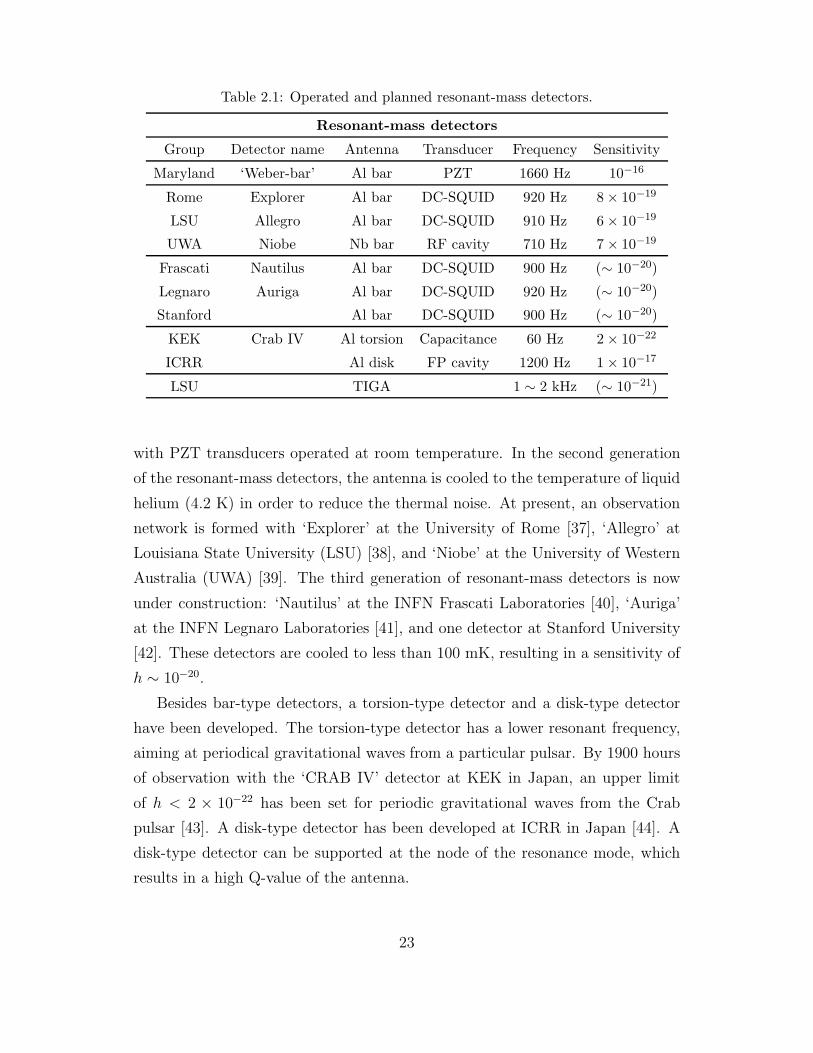
Table 2.1: Operated and planned resonant-mass detectors.
Resonant-mass detectors
Group Detector name Antenna Transducer Frequency Sensitivity
Maryland ‘Weber-bar’ Al bar PZT 1660 Hz 10−16
Rome Explorer Al bar DC-SQUID 920 Hz 8 × 10⁻¹⁹
LSU Allegro Al bar DC-SQUID 910 Hz 6 × 10⁻¹⁹
UWA Niobe Nb bar RF cavity 710 Hz 7 × 10⁻¹⁹
Frascati Nautilus Al bar DC-SQUID 900 Hz (∼ 10−20)
Legnaro Auriga Al bar DC-SQUID 920 Hz (∼ 10−20)
Stanford Al bar DC-SQUID 900 Hz (∼ 10−20)
KEK Crab IV Al torsion Capacitance 60 Hz 2 × 10⁻²²
ICRR Al disk FP cavity 1200 Hz 1 × 10⁻¹⁷
LSU TIGA 1 ∼ 2 kHz (∼ 10−21)
with PZT transducers operated at room temperature. In the second generation
of the resonant-mass detectors, the antenna is cooled to the temperature of liquid
helium (4.2 K) in order to reduce the thermal noise. At present, an observation
network is formed with ‘Explorer’ at the University of Rome [37], ‘Allegro’ at
Louisiana State University (LSU) [38], and ‘Niobe’ at the University of Western
Australia (UWA) [39]. The third generation of resonant-mass detectors is now
under construction: ‘Nautilus’ at the INFN Frascati Laboratories [40], ‘Auriga’
at the INFN Legnaro Laboratories [41], and one detector at Stanford University
[42]. These detectors are cooled to less than 100 mK, resulting in a sensitivity of
h ∼ 10−20.
Besides bar-type detectors, a torsion-type detector and a disk-type detector
have been developed. The torsion-type detector has a lower resonant frequency,
aiming at periodical gravitational waves from a particular pulsar. By 1900 hours
of observation with the ‘CRAB IV’ detector at KEK in Japan, an upper limit
of h < 2 × 10⁻²² has been set for periodic gravitational waves from the Crab
pulsar [43]. A disk-type detector has been developed at ICRR in Japan [44]. A
disk-type detector can be supported at the node of the resonance mode, which
results in a high Q-value of the antenna.
23

The subsequent generation resonant-mass detectors will be ‘sphere-shaped’
detectors called TIGA (a truncated icosahedral gravitational wave antenna) [45,
46]. A TIGA has a larger cross section for gravitational waves. In addition,
the source direction and polarization is determined with a TIGA. The discussed
and planned detector is a network of antennas with different resonant frequencies
(‘xylophone’), cooled to 50 mK. The sensitivity of a ‘xylophone’ of TIGA detectors
is expected to be h ∼ 10−21.
2.3.3 Interferometric detector
Principle of an interferometric detector
The principle of an interferometric gravitational wave detector is a Michelson
interferometer (Fig. 3.1)13. As described in Section 2.1, the distance of free par-
ticles is perturbed by gravitational waves. The change in distance causes a phase
change in the laser light (the phase of the laser beam is modulated by the grav-
itational waves), which is detected as change in the interference fringe of the
Michelson interferometer.
The Michelson interferometer is comprised of a laser source, a beamsplitter,
two mirrors, and a photo detector. In the interferometric detectors on the earth,
the mirrors are suspended as pendulums so that they should behave as free masses
in the direction along the laser beam at the observation frequency. The beam
from the laser source is divided in two orthogonal directions (along x- and y-
directions in Fig. 3.1) with a beamsplitter. The two beams are reflected back with
mirrors and recombined on the beamsplitter, producing an interference fringe.
Gravitational waves change the arm length (distance between a mirror and the
beamsplitter) differentially, i.e., stretch one arm length and shrink the other14.
This change appears as the change of the interference fringe and detected with a
photo detector.
The sensitivity of an interferometric detector is limited by shot noise, thermal
noise, and seismic noise. Since the effect of the shot noise is inversely proportional
13The details of an interferometric detector are discussed in the following Chapters.14This point of view is true when the period of the gravitational waves is lower enough than
the round trip time of the light in the arms.
24

Table 2.2: Currently operated prototype interferometers. FPM: a Fabry-
Perot-Michelson interferometer.
Prototype interferometers
Group Baseline Type Displacement noise
Caltech 40 m Locked Fabry-Perot 3 × 10⁻¹⁹ m/√
Hz (1994)
Power-recycled FPM —
MPQ 30 m Delay-line Michelson 3 × 10⁻¹⁸ m/√
Hz (1988)
Dual-recycled Michelson —
Glasgow 10 m Locked Fabry-Perot 6 × 10⁻¹⁹ m/√
Hz (1992)
NAO 20 m Fabry-Perot Michelson 2 × 10⁻¹⁷ m/√
Hz (1996)
Power-recycled FPM —
Tokyo 3 m Fabry-Perot Michelson 1 × 10⁻¹⁷ m/√
Hz (1994)
Power-recycled FPM 2 × 10⁻¹⁷ m/√
Hz (1998)
to the square-root of the laser power, a power recycling technique is used together
with a high-power laser source. The gravitational wave signal is proportional to
the baseline length of an interferometer, while the thermal noise and seismic noise
are independent of the baseline length. Thus, larger baseline length is desirable
to reduce the effect of thermal noise and seismic noise.
Development of interferometric detectors
The real development of laser interferometric gravitational wave detectors was
begun in the early 1970s [9, 10]. Since that time, several groups have pursued
interferometric detectors, constructing tabletop interferometers and prototype
interferometers with suspended optics. Table 2.2 summarizes the prototype in-
terferometers under investigation currently. The prototype interferometers were
used to investigate the principles of interferometric detectors and their noise be-
havior. In recent years, the configurations of these prototype interferometers
have been changed to those resembling the real gravitational wave detectors: a
power-recycled Fabry-Perot-Michelson interferometer or a dual-recycled Michel-
son interferometer.
Advanced techniques for future interferometers are under investigation now
25
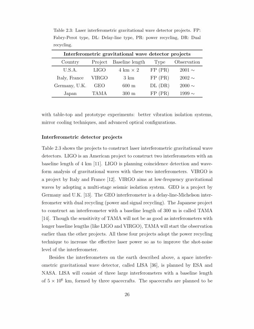
Table 2.3: Laser interferometric gravitational wave detector projects. FP:
Fabry-Perot type, DL: Delay-line type, PR: power recycling, DR: Dual
recycling.
Interferometric gravitational wave detector projects
Country Project Baseline length Type Observation
U.S.A. LIGO 4 km × 2 FP (PR) 2001 ∼Italy, France VIRGO 3 km FP (PR) 2002 ∼
Germany, U.K. GEO 600 m DL (DR) 2000 ∼Japan TAMA 300 m FP (PR) 1999 ∼
with table-top and prototype experiments: better vibration isolation systems,
mirror cooling techniques, and advanced optical configurations.
Interferometric detector projects
Table 2.3 shows the projects to construct laser interferometric gravitational wave
detectors. LIGO is an American project to construct two interferometers with an
baseline length of 4 km [11]. LIGO is planning coincidence detection and wave-
form analysis of gravitational waves with these two interferometers. VIRGO is
a project by Italy and France [12]. VIRGO aims at low-frequency gravitational
waves by adopting a multi-stage seismic isolation system. GEO is a project by
Germany and U.K. [13]. The GEO interferometer is a delay-line-Michelson inter-
ferometer with dual recycling (power and signal recycling). The Japanese project
to construct an interferometer with a baseline length of 300 m is called TAMA
[14]. Though the sensitivity of TAMA will not be as good as interferometers with
longer baseline lengths (like LIGO and VIRGO), TAMA will start the observation
earlier than the other projects. All these four projects adopt the power recycling
technique to increase the effective laser power so as to improve the shot-noise
level of the interferometer.
Besides the interferometers on the earth described above, a space interfer-
ometric gravitational wave detector, called LISA [36], is planned by ESA and
NASA. LISA will consist of three large interferometers with a baseline length
of 5 × 10⁶ km, formed by three spacecrafts. The spacecrafts are planned to be
26

launched in 2008 ∼ 2010.
2.3.4 Other types of gravitational wave detectors
Doppler tracking
Doppler tracking is a scheme to detect gravitational waves by the accurate mea-
surement of the Doppler shift of microwave signals communicated between the
earth and a spacecraft [47]. The output of a stable oscillator on the earth (typ-
ically with a frequency of a few MHz) is up-converted and transmitted to a
spacecraft (up link). This up-linked microwave is sent back to the earth by the
spacecraft (down link). The frequency of the down-linked microwave is measured
by comparison with that of the master oscillator. The fundamental limitation to
the sensitivity of the Doppler tracking scheme is given by the stability of the fre-
quency reference. With the best available frequency standard (a hydrogen maser
clock) the sensitivity is about h ∼ 10−15 (in 1000 sec). The observation band
(10−2 ∼ 10−4 Hz) is restricted by the round-trip time of the radio signal to lower
frequencies and by the thermal noise of the telecommunication system to higher
frequencies.
In an observation about one month long using a ULYSSES spacecraft, the
sensitivity was about
h ∼ 1.3 × 10⁻¹⁵
(f
10−2 Hz
)−0.26
(2.36)
in the frequency band from 2.3 × 10⁻⁴ to 5 × 10⁻² Hz [48, 49]. In this observa-
tion, the sensitivity was limited by the density fluctuations of the inter-planetary
plasma. It is possible to reduce this noise by using multi-frequency or higher
frequency radio links. In a planned mission (CASSINI), the plasma noise will be
decreased by a factor about 250 using higher frequency radio links. With the im-
provements in the reference clock and telecommunication system, the sensitivity
of CASSINI will be h ∼ 7 × 10⁻¹⁶.
Laser interferometer in space
The observation band of a ground-based interferometric detector is limited by
the seismic noise at lower frequencies, where several strong gravitational wave
27
sources are expected: periodic waves from binaries and pulsars, and burst waves
from MBHs. A mission named LISA (Laser Interferometer Space Antenna) is
planned targeting these low frequency gravitational waves (10−4 ∼ 1 Hz) [36].
In LISA, a triangle interferometer with a baseline length of 5 × 10⁶ km will be
formed by three spacecraft in an earth-like heliocentric orbit, following 20 degrees
behind the earth. The spacecraft will monitor the distance to one another using
laser beams in a similar way as the RF transponder scheme.
LISA will have a sensitivity of h ∼ 10−21 at 10−3 Hz with a bandwidth of
10−3 Hz; the sensitivity will be improved much more than that of the Doppler
tracking scheme. The sensitivity of LISA is limited by the optical-path noise (shot
noise, master clock noise, residual laser phase noise, beam pointing instabilities,
and so on) and the forces acting on the proof masses (thermal distortion of space
craft, thermal noise due to dielectric losses, electrical force on charged proof
masses, residual gas impacts on proof masses, and so on).
LISA is envisaged as a NASA/ESA collaborative project. The mission is
aimed at a launch in the 2008∼2010 time frame.
Pulsar timing
Since arrival times of the radio pulses from millisecond and binary pulsars are
measured with a very high accuracy, their fluctuations can be used for the detec-
tion of gravitational waves [50, 51]. The effect of gravitational waves passing by
a pulsar or by the earth appears in the differences of the observed pulse arrival
times and those predicted by the pulsar spindown and so on. The observation
target of pulsar timing is a low-frequency (10−7 ∼ 10−9 Hz) stochastic gravita-
tional wave radiation background, which may be generated in the early universe,
or may exist as the superposition of many low-frequency sources.
The statistical analysis of the pulsar timing data of PSR B1855+09 yields an
upper limit of 9 × 10⁻⁸ for Ωg in a frequency range of 4 × 10⁻⁹ ∼ 4 × 10⁻⁸ Hz
[52]. The observation band is determined by the total observation time (lower
frequency limit) and sufficient integration time of the pulse arrival times (upper
frequency limit). This value corresponds to h ∼ 3 × 10⁻¹⁴ at a frequency of
10−8 Hz.
The sensitivity of pulsar timing is limited by the stability of the pulsar, the
28

long-term frequency stability of the reference clock, and the observation time.
The upper limit of Ωg is improved with the fifth power of the observation time.
An observation network with stable pulsars would alleviate problems with the
reference clock and the effect of the other noise source, inter-stellar scintillation
[3].
29

Chapter 3
Interferometric gravitational
wave detector
Laser interferometric gravitational wave detectors have been investigated and de-
veloped energetically in recent years. This is because an interferometric detector
has a wide observation band, and its potential high sensitivity with a long base-
line length of a few kilometers. In this Chapter, we describe the fundamentals
of an interferometric gravitational wave detector: its characteristics and its noise
sources.
An interferometric gravitational wave detector is comprised of several opti-
cal devices: a Michelson interferometer and cavities. In the LIGO, VIRGO,
and TAMA detectors, the interferometer is formed with a Michelson interfer-
ometer, Fabry-Perot arm cavities, and the recycling cavity. In the first half of
this Chapter, the fundamentals of each optical device are described (a Michelson
interferometer, a Fabry-Perot cavity, and a power recycling technique). In the
latter half, the noise sources of an interferometric gravitational wave detector are
described. This Chapter contains the following Sections.
• Michelson interferometer. The principle of of gravitational wave detec-
tion with a Michelson interferometer. The frequency response of a Michel-
son interferometer and its optimization with delay lines or Fabry-Perot cav-
ities.
• Fabry-Perot cavity. The fundamentals of a Fabry-Perot cavity. The
30
response to a gravitational wave, displacement of a mirror, and fluctuation
of incident laser frequency.
• Power recycling. The principle of power enhancement with power recy-
cling. The characteristics of a power recycling cavity.
• Noise sources for an interferometer. Noise sources which can limit the
sensitivity of an interferometric gravitational wave detector.
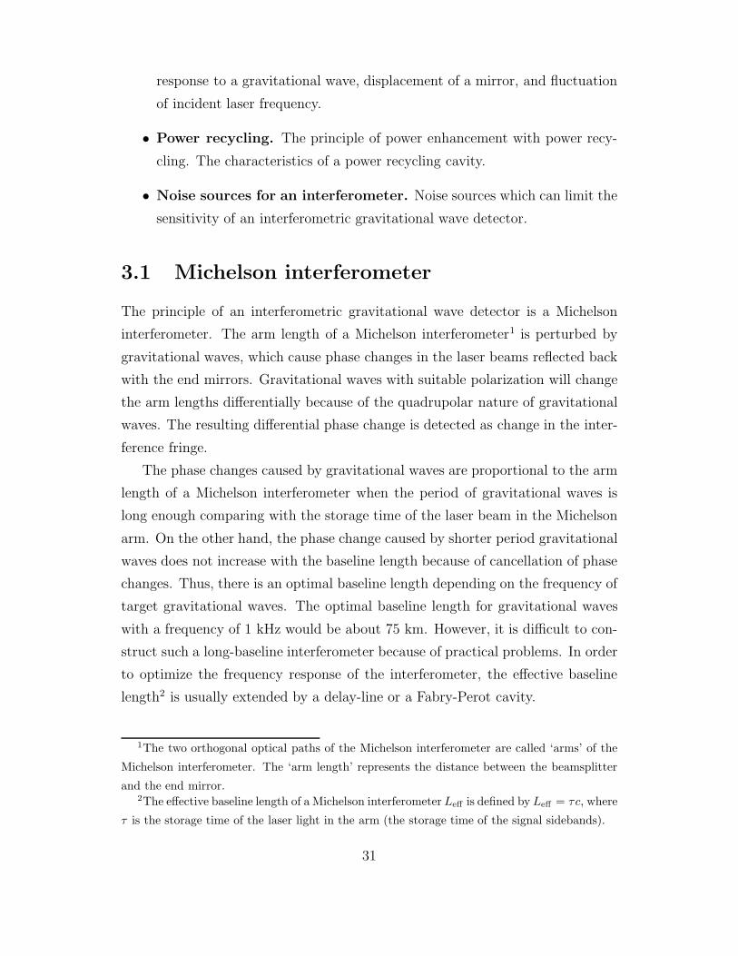
3.1 Michelson interferometer
The principle of an interferometric gravitational wave detector is a Michelson
interferometer. The arm length of a Michelson interferometer1 is perturbed by
gravitational waves, which cause phase changes in the laser beams reflected back
with the end mirrors. Gravitational waves with suitable polarization will change
the arm lengths differentially because of the quadrupolar nature of gravitational
waves. The resulting differential phase change is detected as change in the inter-
ference fringe.
The phase changes caused by gravitational waves are proportional to the arm
length of a Michelson interferometer when the period of gravitational waves is
long enough comparing with the storage time of the laser beam in the Michelson
arm. On the other hand, the phase change caused by shorter period gravitational
waves does not increase with the baseline length because of cancellation of phase
changes. Thus, there is an optimal baseline length depending on the frequency of
target gravitational waves. The optimal baseline length for gravitational waves
with a frequency of 1 kHz would be about 75 km. However, it is difficult to con-
struct such a long-baseline interferometer because of practical problems. In order
to optimize the frequency response of the interferometer, the effective baseline
length2 is usually extended by a delay-line or a Fabry-Perot cavity.
1The two orthogonal optical paths of the Michelson interferometer are called ‘arms’ of the
Michelson interferometer. The ‘arm length’ represents the distance between the beamsplitter
and the end mirror.2The effective baseline length of a Michelson interferometer Leff is defined by Leff = τc, where
τ is the storage time of the laser light in the arm (the storage time of the signal sidebands).
31
Mirror
Mirror
Beamsplitter
Laser source Photo detector
Gravitational wave signal
x
zy
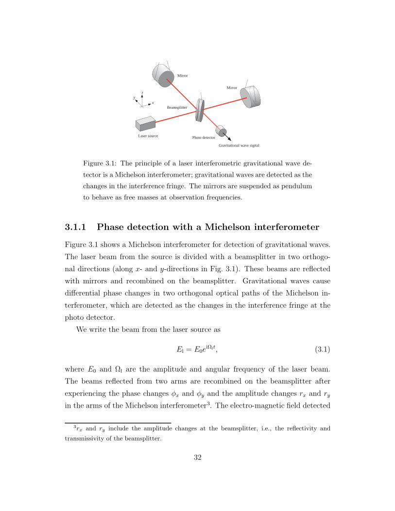
Figure 3.1: The principle of a laser interferometric gravitational wave de-
tector is a Michelson interferometer; gravitational waves are detected as the
changes in the interference fringe. The mirrors are suspended as pendulum
to behave as free masses at observation frequencies.
3.1.1 Phase detection with a Michelson interferometer
Figure 3.1 shows a Michelson interferometer for detection of gravitational waves.
The laser beam from the source is divided with a beamsplitter in two orthogo-
nal directions (along x- and y-directions in Fig. 3.1). These beams are reflected
with mirrors and recombined on the beamsplitter. Gravitational waves cause
differential phase changes in two orthogonal optical paths of the Michelson in-
terferometer, which are detected as the changes in the interference fringe at the
photo detector.
We write the beam from the laser source as
El = E0eiΩlt, (3.1)
where E0 and Ωl are the amplitude and angular frequency of the laser beam.
The beams reflected from two arms are recombined on the beamsplitter after
experiencing the phase changes φx and φy and the amplitude changes rx and ry
in the arms of the Michelson interferometer3. The electro-magnetic field detected
3rx and ry include the amplitude changes at the beamsplitter, i.e., the reflectivity and
transmissivity of the beamsplitter.
32
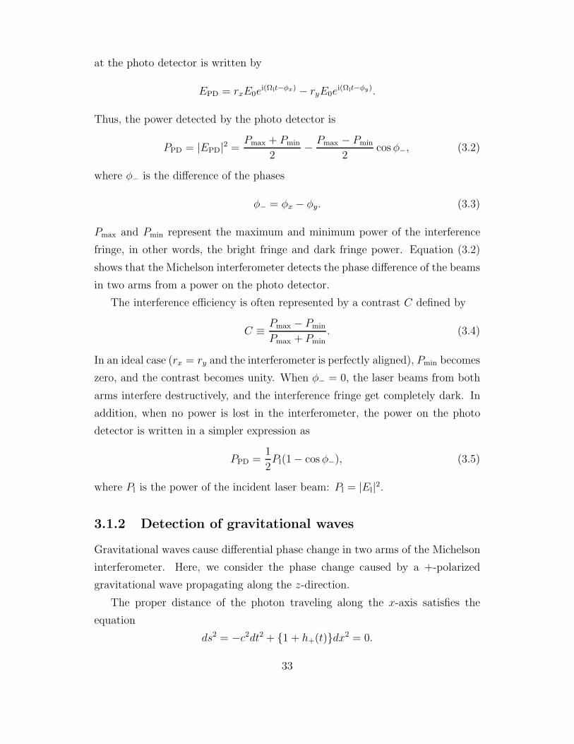
at the photo detector is written by
EPD = rxE0ei(Ωlt−φx) − ryE0e
i(Ωlt−φy).
Thus, the power detected by the photo detector is
PPD = |EPD|2 =Pmax + Pmin
2− Pmax − Pmin
2cos φ−, (3.2)
where φ− is the difference of the phases
φ− = φx − φy. (3.3)
Pmax and Pmin represent the maximum and minimum power of the interference
fringe, in other words, the bright fringe and dark fringe power. Equation (3.2)
shows that the Michelson interferometer detects the phase difference of the beams
in two arms from a power on the photo detector.
The interference efficiency is often represented by a contrast C defined by
C ≡ Pmax − Pmin
Pmax + Pmin. (3.4)
In an ideal case (rx = ry and the interferometer is perfectly aligned), Pmin becomes
zero, and the contrast becomes unity. When φ− = 0, the laser beams from both
arms interfere destructively, and the interference fringe get completely dark. In
addition, when no power is lost in the interferometer, the power on the photo
detector is written in a simpler expression as
PPD =1
2Pl(1 − cos φ−), (3.5)
where Pl is the power of the incident laser beam: Pl = |El|2.
3.1.2 Detection of gravitational waves
Gravitational waves cause differential phase change in two arms of the Michelson
interferometer. Here, we consider the phase change caused by a +-polarized
gravitational wave propagating along the z-direction.
The proper distance of the photon traveling along the x-axis satisfies the
equation
ds2 = −c2dt2 + 1 + h+(t)dx2 = 0.
33
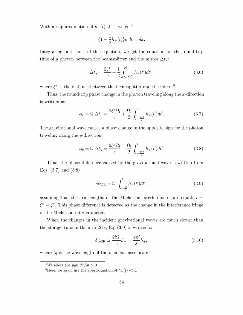
With an approximation of h+(t) 1, we get4
1 − 1
2h+(t)c dt = dx.
Integrating both sides of this equation, we get the equation for the round-trip
time of a photon between the beamsplitter and the mirror ∆tx:
∆tx =2ξx
c+
1
2
∫ t
t− 2ξx
c
h+(t′)dt′, (3.6)
where ξx is the distance between the beamsplitter and the mirror5.
Thus, the round-trip phase change in the photon traveling along the x-direction
is written as
φx = Ωl∆tx =2ξxΩl
c+
Ωl
2
∫ t
t− 2ξx
c
h+(t′)dt′. (3.7)
The gravitational wave causes a phase change in the opposite sign for the photon
traveling along the y-direction:
φy = Ωl∆ty =2ξyΩl
c− Ωl
2
∫ t
t− 2ξy
c
h+(t′)dt′. (3.8)
Thus, the phase difference caused by the gravitational wave is written from
Eqs. (3.7) and (3.8)
δφGR = Ωl
∫ t
t− 2lc
h+(t′)dt′, (3.9)
assuming that the arm lengths of the Michelson interferometer are equal: l =
ξx = ξy . This phase difference is detected as the change in the interference fringe
of the Michelson interferometer.
When the changes in the incident gravitational waves are much slower than
the storage time in the arm 2l/c, Eq. (3.9) is written as
δφGR ' 2lΩl
ch+ =
4πl
λlh+, (3.10)
where λl is the wavelength of the incident laser beam.
4We select the sign dx/dt > 0.5Here, we again use the approximation of h+(t) 1.
34
3.1.3 Frequency response and baseline length
Though the sensitivity of a Michelson interferometer increases with a larger base-
line length for low-frequency gravitational waves, it does not increase for a high
frequency gravitational waves because of cancellation of the phase changes. Thus,
a Michelson interferometer has an optimal baseline length corresponding to the
target frequency of gravitational waves.
By a Fourier transformation of h+(t),
h+(t) =
∫ ∞
−∞h+(ω)eiωtdω. (3.11)
Substituting this equation into Eq. (3.9),
δφGR = Ωl
∫ t
t− 2lc
dt′∫ ∞
−∞dωh+(ω)eiωt′ =
∫ ∞
−∞HMI(ω)h+(ω)eiωtdω, (3.12)
where HMI(ω) is written by
HMI(ω) =2Ωl
ωsin
(lω
c
)e−i lω
c . (3.13)
HMI(ω) represents the sensitivity of the Michelson interferometer to gravitational
waves with an angular frequency of ω.
In an approximation that the period of a gravitational wave (2π/ω) is much
longer than the storage time in the arm of the Michelson interferometer (τ =
2l/c), the absolute value of the response is written as |HMI| ∼ 2Ωll/c; the phase
change caused by gravitational waves is proportional to the baseline length l. This
is because the effect of gravitational waves accumulates during the storage time
of the photon in the arms of the Michelson interferometer. On the other hand,
the sensitivity to higher frequency gravitational waves does not increase with a
larger baseline length because the effects of gravitational waves are integrated
and canceled out.
From Eq. (3.13), we can see that the sensitivity of the Michelson interferometer
is maximized when the baseline length l satisfies
lωobs
c=
π
2, (3.14)
35
Front mirrorEnd mirror
Beamsplitter
Laser source Photo detector
Gravitational wave signal
End mirror
Front mirror
Delay line
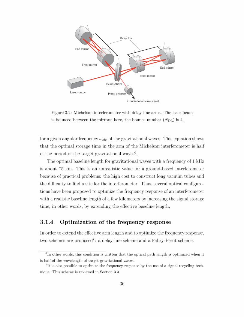
Figure 3.2: Michelson interferometer with delay-line arms. The laser beam
is bounced between the mirrors; here, the bounce number (NDL) is 4.
for a given angular frequency ωobs of the gravitational waves. This equation shows
that the optimal storage time in the arm of the Michelson interferometer is half
of the period of the target gravitational waves6.
The optimal baseline length for gravitational waves with a frequency of 1 kHz
is about 75 km. This is an unrealistic value for a ground-based interferometer
because of practical problems: the high cost to construct long vacuum tubes and
the difficulty to find a site for the interferometer. Thus, several optical configura-
tions have been proposed to optimize the frequency response of an interferometer
with a realistic baseline length of a few kilometers by increasing the signal storage
time, in other words, by extending the effective baseline length.
3.1.4 Optimization of the frequency response
In order to extend the effective arm length and to optimize the frequency response,
two schemes are proposed7: a delay-line scheme and a Fabry-Perot scheme.
6In other words, this condition is written that the optical path length is optimized when it
is half of the wavelength of target gravitational waves.7It is also possible to optimize the frequency response by the use of a signal recycling tech-
nique. This scheme is reviewed in Section 3.3.
36
Front mirror
End mirror
Beamsplitter
Laser source Photo detector
Gravitational wave signal
End mirror
Front mirror
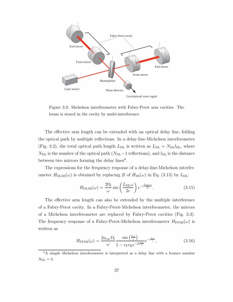
Fabry-Perot cavity
Figure 3.3: Michelson interferometer with Fabry-Perot arm cavities. The
beam is stored in the cavity by multi-interference.
The effective arm length can be extended with an optical delay line, folding
the optical path by multiple reflections. In a delay-line-Michelson interferometer
(Fig. 3.2), the total optical path length LDL is written as LDL = NDLlDL, where
NDL is the number of the optical path (NDL−1 reflections), and lDL is the distance
between two mirrors forming the delay lines8.
The expressions for the frequency response of a delay-line-Michelson interfer-
ometer HDLMI(ω) is obtained by replacing 2l of HMI(ω) in Eq. (3.13) by LDL:
HDLMI(ω) =2Ωl
ωsin
(LDLω
2c
)e−i
LDLω
2c . (3.15)
The effective arm length can also be extended by the multiple interference
of a Fabry-Perot cavity. In a Fabry-Perot-Michelson interferometer, the mirrors
of a Michelson interferometer are replaced by Fabry-Perot cavities (Fig. 3.3).
The frequency response of a Fabry-Perot-Michelson interferometer HFPMI(ω) is
written as
HFPMI(ω) =2acavΩl
ω
sin(
Lωc
)1 − rFrEe−2i Lω
c
e−iLωc , (3.16)
8A simple Michelson interferometer is interpreted as a delay line with a bounce number
NDL = 2.
37
100 101 102 103 104 10510–2
10–1
100
101
102
103
Frequency [Hz]
Res
pons
e
Fabry–Perot–Michelson
Delay–line–Michelson
Michelson
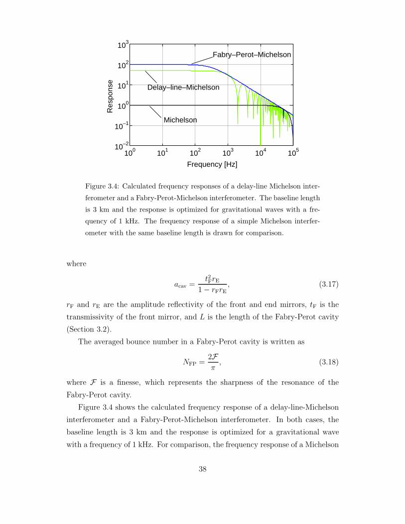
Figure 3.4: Calculated frequency responses of a delay-line Michelson inter-
ferometer and a Fabry-Perot-Michelson interferometer. The baseline length
is 3 km and the response is optimized for gravitational waves with a fre-
quency of 1 kHz. The frequency response of a simple Michelson interfer-
ometer with the same baseline length is drawn for comparison.
where
acav =t2FrE
1 − rFrE, (3.17)
rF and rE are the amplitude reflectivity of the front and end mirrors, tF is the
transmissivity of the front mirror, and L is the length of the Fabry-Perot cavity
(Section 3.2).
The averaged bounce number in a Fabry-Perot cavity is written as
NFP =2Fπ
, (3.18)
where F is a finesse, which represents the sharpness of the resonance of the
Fabry-Perot cavity.
Figure 3.4 shows the calculated frequency response of a delay-line-Michelson
interferometer and a Fabry-Perot-Michelson interferometer. In both cases, the
baseline length is 3 km and the response is optimized for a gravitational wave
with a frequency of 1 kHz. For comparison, the frequency response of a Michelson
38
Front mirror End mirrorEi
Er
Ea
Eb
Et
L
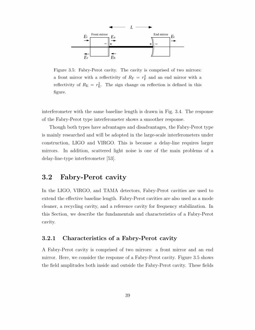
Figure 3.5: Fabry-Perot cavity. The cavity is comprised of two mirrors:
a front mirror with a reflectivity of RF = r2F and an end mirror with a
reflectivity of RE = r2E. The sign change on reflection is defined in this
figure.
interferometer with the same baseline length is drawn in Fig. 3.4. The response
of the Fabry-Perot type interferometer shows a smoother response.
Though both types have advantages and disadvantages, the Fabry-Perot type
is mainly researched and will be adopted in the large-scale interferometers under
construction, LIGO and VIRGO. This is because a delay-line requires larger
mirrors. In addition, scattered light noise is one of the main problems of a
delay-line-type interferometer [53].
3.2 Fabry-Perot cavity
In the LIGO, VIRGO, and TAMA detectors, Fabry-Perot cavities are used to
extend the effective baseline length. Fabry-Perot cavities are also used as a mode
cleaner, a recycling cavity, and a reference cavity for frequency stabilization. In
this Section, we describe the fundamentals and characteristics of a Fabry-Perot
cavity.
3.2.1 Characteristics of a Fabry-Perot cavity
A Fabry-Perot cavity is comprised of two mirrors: a front mirror and an end
mirror. Here, we consider the response of a Fabry-Perot cavity. Figure 3.5 shows
the field amplitudes both inside and outside the Fabry-Perot cavity. These fields
39
satisfy the following equations.
Ea = tFEi + rFEb
Eb = rEe−i2LΩl
c Ea
Er = −rFEi + tFEb
Et = tEe−iLΩl
c Ea,
where Ωl is angular frequency of the input laser beam, L is the length of the cavity.
r and t represent the amplitude reflectivity and transmissivity, respectively. The
indices ‘F’ and ‘E’ denote the front mirror and the end mirror, respectively.
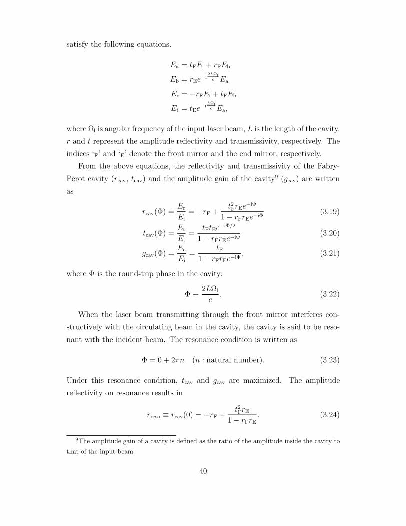
From the above equations, the reflectivity and transmissivity of the Fabry-
Perot cavity (rcav, tcav) and the amplitude gain of the cavity9 (gcav) are written
as
rcav(Φ) =Er
Ei= −rF +
t2FrEe−iΦ
1 − rFrEe−iΦ(3.19)
tcav(Φ) =Et
Ei=
tFtEe−iΦ/2
1 − rFrEe−iΦ(3.20)
gcav(Φ) =Ea
Ei=
tF1 − rFrEe−iΦ
, (3.21)
where Φ is the round-trip phase in the cavity:
Φ ≡ 2LΩl
c. (3.22)
When the laser beam transmitting through the front mirror interferes con-
structively with the circulating beam in the cavity, the cavity is said to be reso-
nant with the incident beam. The resonance condition is written as
Φ = 0 + 2πn (n : natural number). (3.23)
Under this resonance condition, tcav and gcav are maximized. The amplitude
reflectivity on resonance results in
rreso ≡ rcav(0) = −rF +t2FrE
1 − rFrE. (3.24)
9The amplitude gain of a cavity is defined as the ratio of the amplitude inside the cavity to
that of the input beam.
40
3.2.2 Coupling of a cavity
The sign of the reflectivity of a Fabry-Perot cavity on resonance depends on the
coupling of the cavity. The reflectivity of a Fabry-Perot cavity on resonance,
Eq. (3.24), is comprised of two terms: the first term represents the beam directly
reflected from the front mirror, and the second term represents the beam leaking
from inside the cavity. The sign of these terms are opposite.
By neglecting the loss of the front mirror (r2F + t2F = 1), Eq. (3.24) is written
as
rreso ' −rF + rE
1 − rFrE
. (3.25)
When rF > rE, the reflected beam is dominated by the directly-reflected beam
with the front mirror. This cavity is called under-coupled. On the other hand, a
cavity with rF < rE is called over-coupled. In an over-coupled cavity, the reflected
beam is dominated by the beam leaking from inside the cavity. The sign of the
amplitude reflectivity of the cavity differs from each other in under- and over-
coupled cavities. Arm cavities of the Michelson interferometer are usually set to
be over-coupled so that the phase change signal generated inside the arm cavities
should effectively leak to the detection port. In addition, rE is usually set as high
as possible to obtain a high recycling gain.
The reflectivity of a cavity on resonance is zero when rF = rE. This case is
called optimal-coupled. An optimal-coupled cavity transmits all of the incident
beam (if losses in the mirrors are neglected)10. This configuration is used in a
mode cleaner.
The sign of the signal extracted from a power-recycled interferometer depends
on the coupling of the recycling cavity. Moreover, the coupling of the recycling
cavity plays an important role in the signal mixing and separation, which is
described in detail in Chapter 4.
10This is easily shown in Eq. (3.26) by putting rF = rE and Φ = 0.
41
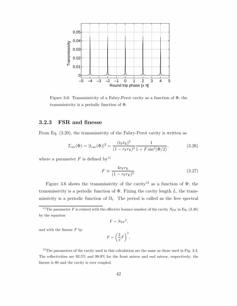
–5 –4 –3 –2 –1 0 1 2 3 4 50
0.01
0.02
0.03
0.04
0.05
Tra
nsm
issi
vity
Round trip phase [x π]
Figure 3.6: Transmissivity of a Fabry-Perot cavity as a function of Φ; the
transmissivity is a periodic function of Φ.
3.2.3 FSR and finesse
From Eq. (3.20), the transmissivity of the Fabry-Perot cavity is written as
Tcav(Φ) = |tcav(Φ)|2 =(tFtE)2
(1 − rFrE)2
1
1 + F sin2(Φ/2), (3.26)
where a parameter F is defined by11
F ≡ 4rFrE
(1 − rFrE)2. (3.27)
Figure 3.6 shows the transmissivity of the cavity12 as a function of Φ; the
transmissivity is a periodic function of Φ. Fixing the cavity length L, the trans-
missivity is a periodic function of Ωl. The period is called as the free spectral
11The parameter F is related with the effective bounce number of the cavity NFP in Eq. (3.48)
by the equation
F = NFP2,
and with the finesse F by
F =(
2πF)2
.
12The parameters of the cavity used in this calculation are the same as those used in Fig. 3.4.
The reflectivities are 92.5% and 99.9% for the front mirror and end mirror, respectively; the
finesse is 80 and the cavity is over coupled.
42
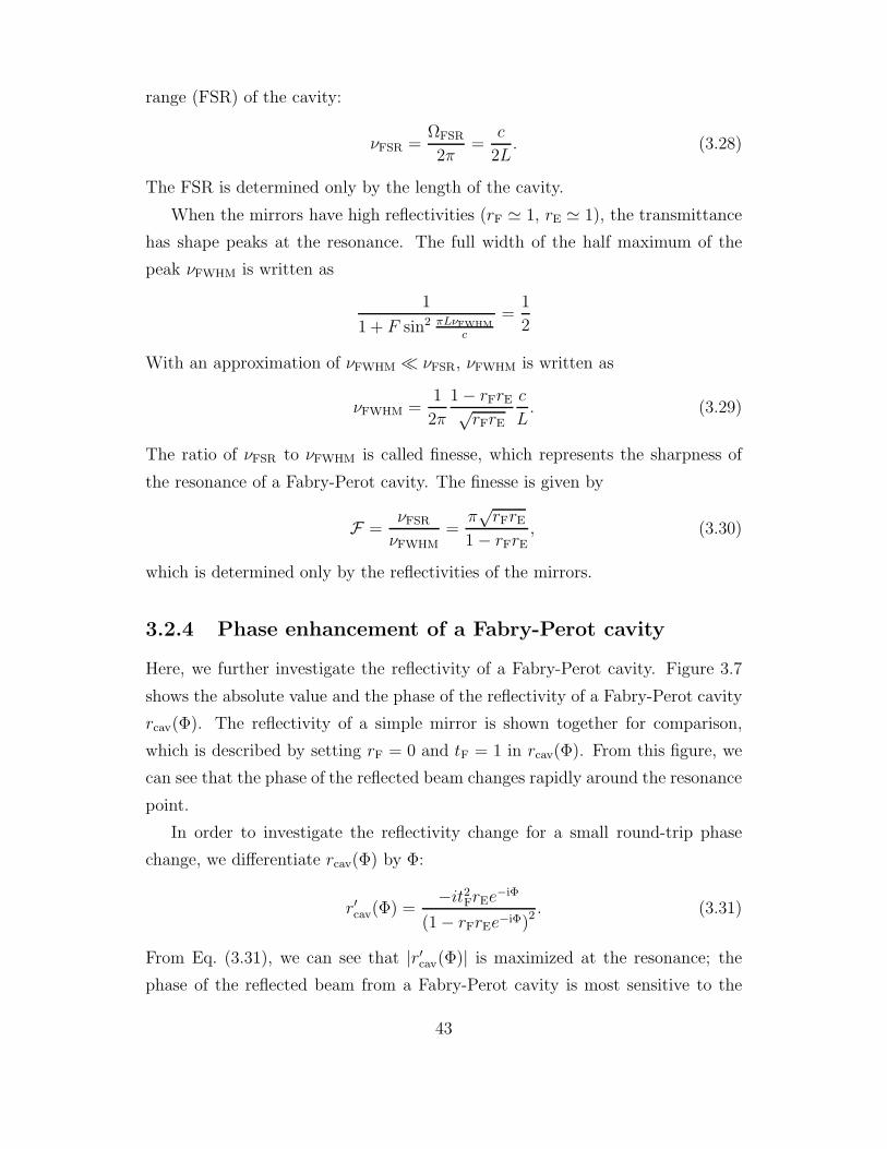
range (FSR) of the cavity:
νFSR =ΩFSR
2π=
c
2L. (3.28)
The FSR is determined only by the length of the cavity.
When the mirrors have high reflectivities (rF ' 1, rE ' 1), the transmittance
has shape peaks at the resonance. The full width of the half maximum of the
peak νFWHM is written as
1
1 + F sin2 πLνFWHM
c
=1
2
With an approximation of νFWHM νFSR, νFWHM is written as
νFWHM =1
2π
1 − rFrE√rFrE
c
L. (3.29)
The ratio of νFSR to νFWHM is called finesse, which represents the sharpness of
the resonance of a Fabry-Perot cavity. The finesse is given by
F =νFSR
νFWHM=
π√
rFrE
1 − rFrE, (3.30)
which is determined only by the reflectivities of the mirrors.
3.2.4 Phase enhancement of a Fabry-Perot cavity
Here, we further investigate the reflectivity of a Fabry-Perot cavity. Figure 3.7
shows the absolute value and the phase of the reflectivity of a Fabry-Perot cavity
rcav(Φ). The reflectivity of a simple mirror is shown together for comparison,
which is described by setting rF = 0 and tF = 1 in rcav(Φ). From this figure, we
can see that the phase of the reflected beam changes rapidly around the resonance
point.
In order to investigate the reflectivity change for a small round-trip phase
change, we differentiate rcav(Φ) by Φ:
r′cav(Φ) =−it2FrEe−iΦ
(1 − rFrEe−iΦ)2 . (3.31)
From Eq. (3.31), we can see that |r′cav(Φ)| is maximized at the resonance; the
phase of the reflected beam from a Fabry-Perot cavity is most sensitive to the
43
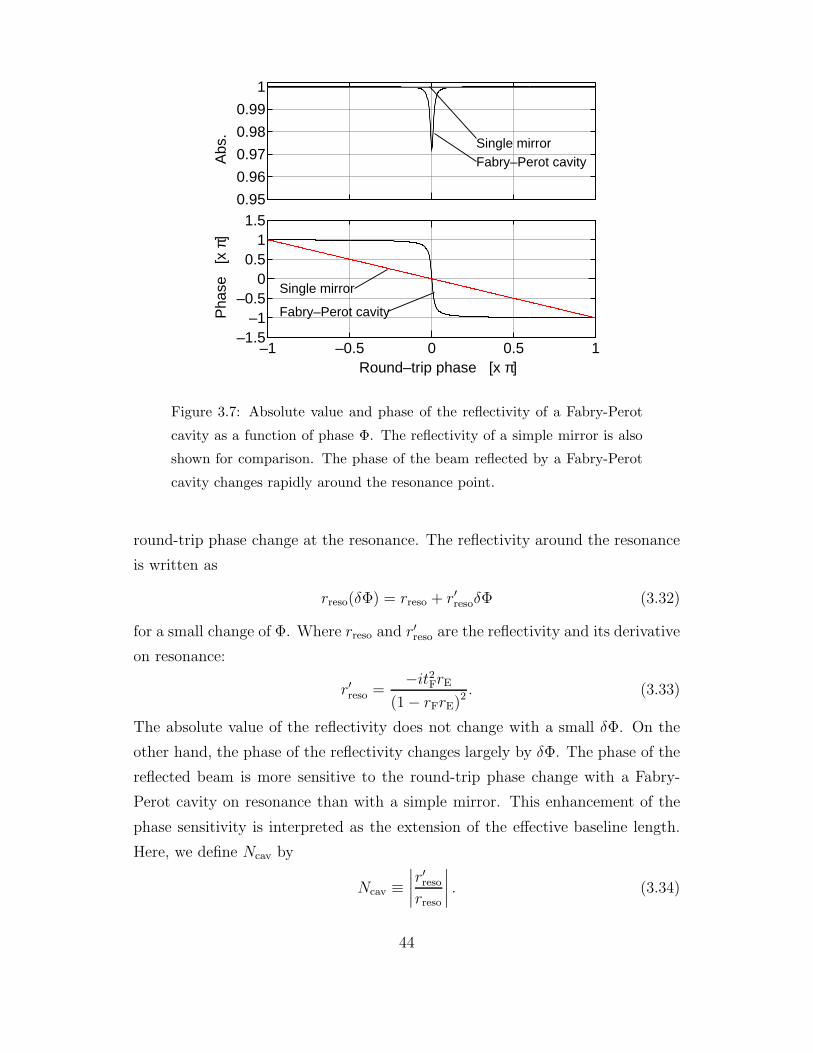
0.95
0.96
0.97
0.98
0.99
1
–1 –0.5 0 0.5 1–1.5
–1–0.5
00.5
11.5
Abs
.P
hase
[x
π]
Round–trip phase [x π]
Fabry–Perot cavitySingle mirror
Single mirror
Fabry–Perot cavity
Figure 3.7: Absolute value and phase of the reflectivity of a Fabry-Perot
cavity as a function of phase Φ. The reflectivity of a simple mirror is also
shown for comparison. The phase of the beam reflected by a Fabry-Perot
cavity changes rapidly around the resonance point.
round-trip phase change at the resonance. The reflectivity around the resonance
is written as
rreso(δΦ) = rreso + r′resoδΦ (3.32)
for a small change of Φ. Where rreso and r′reso are the reflectivity and its derivative
on resonance:
r′reso =−it2FrE
(1 − rFrE)2 . (3.33)
The absolute value of the reflectivity does not change with a small δΦ. On the
other hand, the phase of the reflectivity changes largely by δΦ. The phase of the
reflected beam is more sensitive to the round-trip phase change with a Fabry-
Perot cavity on resonance than with a simple mirror. This enhancement of the
phase sensitivity is interpreted as the extension of the effective baseline length.
Here, we define Ncav by
Ncav ≡∣∣∣∣r′resorreso
∣∣∣∣ . (3.34)
44

Ncav is called the effective bounce number of the cavity because the phase change
of the beam reflected by a Fabry-Perot cavity is enhanced by a factor of Ncav,
comparing that reflected by a simple mirror13.
3.2.5 Response to gravitational waves
As described before, the response of a Fabry-Perot cavity to gravitational waves
has a frequency dependence. We discuss the frequency response of a Fabry-Perot
cavity here14.
The time taken for a photon to make n-times’ round-trips between two mirrors
is written in the same manner as Eq. (3.6):
∆tn ' 2L
cn +
1
2
∫ t
t− 2Lc
n
h+(t′)dt′, (3.35)
for the cavity with length L along x-direction. This equation is rewritten with a
Fourier transformation Eq. (3.11) as
∆tn ' 2L
cn +
1
2
∫ ∞
−∞h+(ω)
1 − e−2i Lωc
n
iωeiωtdω. (3.36)
Then, the beam reflected by the Fabry-Perot cavity is written as superposition
of the multi-reflected beams:
Er = Ei
−rF + t2FrE
∞∑n=1
(rFrE)n−1e−iΩl∆tn
. (3.37)
Substituting ∆tn in Eq. (3.36), and using the approximation |h+| 1, we obtain
rcav(Φ, ω) = −rF +t2FrEe−iΦ
1 − rFrEe−iΦ
− t2FrEe−iΦ
1 − rFrEe−iΦ
∫ ∞
−∞
Ωl
2ωh+(ω)
1 − e−2iγ
1 − rErFe−iΦe−2iγeiωtdω, (3.38)
where
γ ≡ Lω
c. (3.39)
13The reflectivity can be written as r = ae−iNΦ, where a is a constant number and N is a
phase enhancement factor. From this expression, we obtain the relation N =∣∣∣ r′
r
∣∣∣.14Here, we consider the same gravitational waves as before: +-polarized gravitational waves
propagating along the z-direction.
45

In the case that the incident beam is resonant with the cavity (Φ = 0), the
reflectivity is written as
rreso(ω) = rreso − i
∫ ∞
−∞HFP(ω)h+(ω)eiωtdω, (3.40)
where HFP(ω) is the frequency response function of a Fabry-Perot cavity to grav-
itational waves15
HFP(ω) =acavΩl
ω
sin γ
1 − rFrEe−2iγe−iγ, (3.41)
acav =t2FrE
1 − rFrE
. (3.42)
Since the gravitational waves cause phase changes of opposite sign in the y-
direction, the frequency response function is doubled for the Fabry-Perot-Michelson
interferometer, written as16
HFPMI = 2HFP(ω). (3.43)
3.2.6 Storage time
With a good approximation that the changes in gravitational waves are small
enough within the round-trip time in the cavity (γ = ωLc
1), the frequency
response is written as
|HFP(ω)| =acavΩlL
c(1 − rFrE)
1√1 + (τω)2
, (3.44)
where τ is an average storage time of a photon in the cavity
τ =
√FL
c=
2L
c
√rFrE
(1 − rFrE). (3.45)
15The second term of Eq. (3.40) does not represent the phase change on the reflection, but
the sideband produced by the phase modulation by gravitational waves.16When the arm lengths are equal in Michelson and Fabry-Perot-Michelson interferometers,
the ratio of the response functions reduces to the phase-enhancement factor of the Fabry-Perot
cavity in the limit ω → 0:
limω→0
HFPMI
HMI= lim
ω→0
acav
1 − rFrEe−2iγ= |r′reso|.
46

Equation (3.44) shows that the cavity is a low-pass filter with a cutoff frequency
of
νc =ωc
2π=
1
2πτ. (3.46)
The storage time τ in Eq. (3.45) is written using the finesse expressed by
Eq. (3.30):
τ =2L
πcF . (3.47)
In addition, since τ can be considered as the average storage time in a cavity, the
effective bounce number NFP is defined by the equation
τ = NFPL
c.
From this equation, NFP is expressed by the finesse:
NFP =cτ
L=
2Fπ
. (3.48)
3.2.7 Response to mirror displacement
In practice, the phase of the beam reflected from a Fabry-Perot cavity is also
changed by the motion of the mirrors caused by noise such as seismic noise and
thermal noise. In this part, we show the response of a cavity to the mirror motion.
The time taken for a photon to make n-times’ round-trips in the cavity is
written as
∆tn ' 2L
cn +
2
c
n∑m=1
δL(t− 1c(2m−1)L) (3.49)
with the approximation of δL(t) L. With a Fourier transformation expressed
by
δL(t) =
∫ ∞
−∞δL(ω)eiωtdω,
the equation is rewritten as
∆tn ' 2L
cn +
2
c
∫ ∞
−∞δL(ω)
1 − e−2iγn
eiγ − e−iγeiωtdω. (3.50)
47

Substrating this expression for ∆tn to
rcav = −rF + t2FrE
∞∑n=1
(rFrE)n−1e−iΩl∆tn
and using an approximation δL(ω) 1, we obtain
rcav(Φ, ω) = −rF + t2FrE
∞∑n=1
(rFrE)n−1e−2iLΩl
cn
1 − i
2Ωl
c
∫ ∞
−∞δL(ω)
1 − e−2iγn
eiγ − e−iγeiωtdω
= −rF +t2FrEe−iΦ
1 − rFrEe−iΦ
−it2FrEe−iΦ
1 − rFrEe−iΦ
∫ ∞
−∞
2Ωl
cδL(ω)
e−iγ
1 − rFrEe−iΦe−2iγeiωtdω (3.51)
When the input beam is resonant with the cavity, the reflectivity is written as
rreso(ω) = rreso − i
∫ ∞
−∞H
(L)FP (ω)δL(ω)eiωtdω, (3.52)
where H(L)FP (ω) is the response of a Fabry-Perot cavity to the change in the cavity
length:
H(L)FP (ω) =
2acavΩl
c
e−iγ
1 − rFrEe−2iγ. (3.53)
H(L)FP (ω) is related with the response to gravitational waves HFP(ω) by
H(L)FP (ω) =
2ω
c sin γHFP(ω) ' 2
LHFP(ω). (3.54)
This relation means that the response of the cavity to a cavity length change δL
is equal to the response to gravitational waves with an amplitude 2δL/L. In other
words, the response of a Fabry-Perot-Michelson interferometer to the differential
length change in two cavities δL− is equal to the response to gravitational waves
with an amplitude
h+ =δL−L
. (3.55)
3.2.8 Response to frequency fluctuation
Fabry-Perot cavity is also sensitive to a frequency fluctuation of the input laser
beam. Here, we consider the response of a Fabry-Perot cavity to a laser frequency
noise.
48

A frequency noise δν(t) has a following relation with a phase noise of the laser
source δφ(t):
δν(t) =1
2π
∂φ(t)
∂t. (3.56)
In a case that the phase noise is small enough, δφ(t) 1, the incident laser
beam is written as
Ein = E0eiΩlt+δφ(t) = E0e
iΩlt1 + iδφ(t). (3.57)
This equation is rewritten as
Ein = E0eiΩlt + iE0
∫ ∞
−∞δφ(ω)ei(Ωl+ω)tdω, (3.58)
using a Fourier transformation
δφ(t) =
∫ ∞
−∞δφ(ω)eiωtdω.
Then the reflected beam by a Fabry-Perot cavity, Er, is written as
Er = E0rcav(Φ)eiΩlt + iE0
∫ ∞
−∞δφ(ω)rcav(Φω)ei(Ωl+ω)tdω, (3.59)
where
Φω =2L(Ωl + ω)
c= Φ + 2γ.
From Eq. (3.59), we obtain with an approximation δφ(t) 1,
Er = E0rcav(Φ)eiΩt+δφ(t) + iE0
∫ ∞
−∞rcav(Φω) − rcav(Φ) δφ(ω)ei(Ωl+ω)tdω
' Einrcav(Φ)
+Eint2FrEe−iΦ
1 − rFrEe−iΦ
∫ ∞
−∞
2 sin γ
1 − rFrEe−i(Φ+2γ)e−iγδφ(ω)eiωtdω. (3.60)
Under a resonant condition of the cavity17,
rreso(ω) = rreso − i
∫ ∞
−∞H
(F)FP (ω)δν(ω)eiωtdω, (3.61)
17From Eq. (3.56), we have a relation
δφ(ω) =2πδν(ω)
iω.
49

Compound mirror
Recycling mirrorEeff
Ecir
Einc
Eref
Figure 3.8: Recycling cavity formed by a recycling mirror and a compound
mirror. Fields around are defined at the recycling mirror.
where H(F)FP (ω) is a frequency response function of a Fabry-Perot cavity to a
frequency fluctuation:
H(F)FP (ω) =
4πacav
ω
sin γ
1 − rFrEe−2iγe−iγ. (3.62)
H(F)FP (ω) has a following relation with H
(L)FP (ω) when γ is small enough:
H(L)FP (ω) ' νl
LH
(F)FP (ω), (3.63)
where νl is a frequency of the laser source (νl = Ωl/2π). From Eq. (3.63) a
frequency noise δνl cause a same noise as
δL =δνl
νlL. (3.64)
3.3 Power recycling
3.3.1 Principle of power recycling
Shot noise is one of fundamental noises which limit the sensitivity of an inter-
ferometer. Shot noise is a photon counting error, which is proportional to the
square-root of the laser power incident in the interferometer. Since the gravita-
tional wave signal is proportional to the incident power, the shot-noise level of
an interferometer is improved with a high laser power.
Besides increasing the laser-source power, the shot-noise level is improved by
a technique called power recycling [15]. In order to realize the best shot-noise
level, an interferometric gravitational wave detector is usually operated under a
50

dark fringe condition; the reflected beams by the arm mirrors (or cavities) are set
to interfere destructively at the detection port. In this case, most of the injected
laser power is reflected back toward the laser source if the losses of the interfer-
ometer is low enough. This back-reflected beam is reused by reflecting back into
the interferometer with a partial mirror inserted between the laser source and
the interferometer, which results in the increase of power in the interferometer.
This scheme is called power recycling, and the inserted mirror is called a power
recycling mirror.
In another point of view, power recycling is considered to be a formation of an
additional cavity, called a recycling cavity (Fig. 3.8). A Michelson interferometer
operated at the dark fringe is considered to be a high-reflective compound mirror.
The recycling mirror forms a recycling cavity with this compound mirror; the
power in the cavity is enhanced when the cavity is resonant with the input laser
beam.
3.3.2 Recycling cavity
Considering the recycling cavity as a Fabry-Perot cavity, the amplitude reflectiv-
ity and gain is written in the same way as Section 3.2. The compound mirror
forms a recycling cavity together with the recycling mirror (Fig. 3.8). The fields
around the recycling cavity have the relations
Eeff = tREinc + rREcir
Ecir = rcomEeff
Eref = −rREinc + tREcir,
where index ‘R’ denotes the recycling mirror. rcom is an complex reflectivity of
the compound mirror; the absolute value and the phase represent the amplitude
reflectivity and phase change on reflection, respectively. From above equations,
we obtain the expressions for the amplitude gain of the recycling cavity g and the
reflectivity of the recycling cavity rrec:
g =Eeff
Einc=
tR1 − rRrcom
(3.65)
rrec =Eref
Einc= −rR +
t2Rrcom
1 − rRrcom. (3.66)
51

0.5 0.6 0.7 0.8 0.9 1
100
101
102
Rec
yclin
g ga
in
Reflectivity of the recycling mirror
1–Rcom=0.01
1–Rcom=0.032
1–Rcom=0.32
1–Rcom=0.1
Maximum recycling gain
Figure 3.9: Power recycling gain as a function of the reflectivity of the
recycling mirror for given reflectivities of the compound mirror. The power
recycling gain is maximized when the reflectivity of the recycling mirror is
equal to that of the compound mirror.
The incident beam is resonate with the recycling cavity when rcom is a real and
positive number.
3.3.3 Power recycling gain
The ratio of the laser power on the beamsplitter with and without the recycling
mirror, G, is called a power recycling gain or a power recycling factor:
G = g2 =t2R
(1 − rRrcom)2. (3.67)
When G > 1, the effective power of the laser source, i.e., the laser power incident
on the interferometer, increases to GPl, and the shot-noise level is improved by√G. Figure 3.9 shows a power recycling gain as a function of the reflectivity of
the recycling mirror (RR) for given reflectivities of a compound mirror (Rcom =
|rcom|2). The power recycling gain is maximized when the reflectivity of the
52

recycling mirror is equal to that of the compound mirror18:
RR = Rcom. (3.68)
Under this condition, the recycling cavity is considered to be a Fabry-Perot cavity
comprised of mirrors with a same reflectivity; all of the input power is transmits
through or lost in the recycling cavity. Equation (3.67) is written with the reso-
nant condition and Eq. (3.68) as
Gmax =1
1 − Rcom. (3.69)
1 − Rcom is a total loss in the compound mirror: scattering, absorption, finite
reflectivity of the end mirrors (or arm cavities), imperfect interference on the
beamsplitter, and wave-front distortions19. Equation (3.69) shows that the maxim
power recycling gain is inverse proportional to the total loss of the compound
mirror.
3.4 Noise sources for an interferometer
The sensitivity of an interferometric gravitational detector can be easily degraded
by a lot of noise sources. The fundamental noises for a ground-based interferom-
eter are shot noise, thermal noise, and seismic noise. In this Section, we describe
these fundamental noises and other main noise sources.
3.4.1 Optical readout noise
The sensitivity of an optical measurement system like an interferometric gravita-
tional wave detector is limited by the optical readout noise: the shot noise and
the radiation pressure noise [54].
Shot noise
Shot noise is one of fundamental noises which limit the sensitivity of an interfer-
ometer. Michelson interferometer converts differential phase changes in its arms18We neglect the loss in the recycling mirror here.19The wave front of a laser beam is distorted on reflection on and transmission through optics
of the interferometer. This distortions are considered to be a scattering from the TEM00 mode
to higher modes.
53
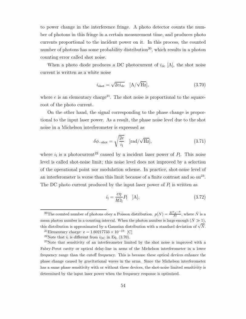
to power change in the interference fringe. A photo detector counts the num-
ber of photons in this fringe in a certain measurement time, and produces photo
currents proportional to the incident power on it. In this process, the counted
number of photons has some probability distribution20, which results in a photon
counting error called shot noise.
When a photo diode produces a DC photocurrent of idc [A], the shot noise
current is written as a white noise
ishot =√
2eidc [A/√
Hz], (3.70)
where e is an elementary charge21. The shot noise is proportional to the square-
root of the photo current.
On the other hand, the signal corresponding to the phase change is propor-
tional to the input laser power. As a result, the phase noise level due to the shot
noise in a Michelson interferometer is expressed as
δφ−shot =
√2e
il[rad/
√Hz], (3.71)
where il is a photocurrent22 caused by a incident laser power of Pl. This noise
level is called shot-noise limit; this noise level does not improved by a selection
of the operational point nor modulation scheme. In practice, shot-noise level of
an interferometer is worse than this limit because of a finite contrast and so on23.
The DC photo current produced by the input laser power of Pl is written as
il =eη
~ΩlPl [A], (3.72)
20The counted number of photons obey a Poisson distribution. p(N) = NN e−N
N! , where N is a
mean photon number in a counting interval. When the photon number is large enough (N 1),
this distribution is approximated by a Gaussian distribution with a standard deviation of√
N .21Elementary charge: e = 1.60217733 × 10⁻¹⁹ [C]22Note that il is different from iDC in Eq. (3.70).23Note that sensitivity of an interferometer limited by the shot noise is improved with a
Fabry-Perot cavity or optical delay-line in arms of the Michelson interferometer in a lower
frequency range than the cutoff frequency. This is because these optical devices enhance the
phase change caused by gravitational waves in the arms. Since the Michelson interferometer
has a same phase sensitivity with or without these devices, the shot-noise limited sensitivity is
determined by the input laser power when the frequency response is optimized.
54
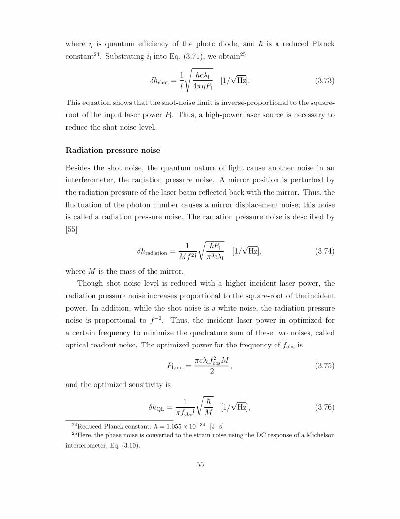
where η is quantum efficiency of the photo diode, and ~ is a reduced Planck
constant24. Substrating il into Eq. (3.71), we obtain25
δhshot =1
l
√~cλl
4πηPl[1/
√Hz]. (3.73)
This equation shows that the shot-noise limit is inverse-proportional to the square-
root of the input laser power Pl. Thus, a high-power laser source is necessary to
reduce the shot noise level.
Radiation pressure noise
Besides the shot noise, the quantum nature of light cause another noise in an
interferometer, the radiation pressure noise. A mirror position is perturbed by
the radiation pressure of the laser beam reflected back with the mirror. Thus, the
fluctuation of the photon number causes a mirror displacement noise; this noise
is called a radiation pressure noise. The radiation pressure noise is described by
[55]
δhradiation =1
Mf2l
√~Pl
π3cλl[1/
√Hz], (3.74)
where M is the mass of the mirror.
Though shot noise level is reduced with a higher incident laser power, the
radiation pressure noise increases proportional to the square-root of the incident
power. In addition, while the shot noise is a white noise, the radiation pressure
noise is proportional to f−2. Thus, the incident laser power in optimized for
a certain frequency to minimize the quadrature sum of these two noises, called
optical readout noise. The optimized power for the frequency of fobs is
Pl ,opt =πcλlf
2obsM
2, (3.75)
and the optimized sensitivity is
δhQL =1
πfobsl
√~
M[1/
√Hz], (3.76)
24Reduced Planck constant: ~ = 1.055 × 10⁻³⁴ [J · s]25Here, the phase noise is converted to the strain noise using the DC response of a Michelson
interferometer, Eq. (3.10).
55
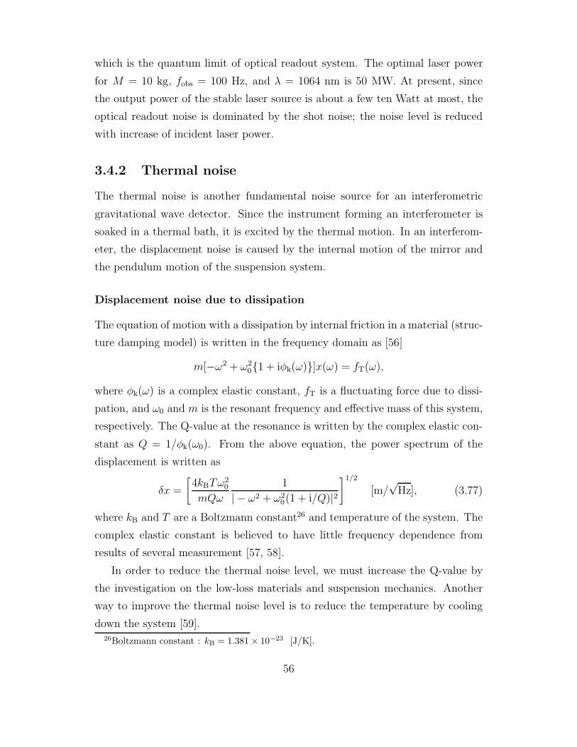
which is the quantum limit of optical readout system. The optimal laser power
for M = 10 kg, fobs = 100 Hz, and λ = 1064 nm is 50 MW. At present, since
the output power of the stable laser source is about a few ten Watt at most, the
optical readout noise is dominated by the shot noise; the noise level is reduced
with increase of incident laser power.
3.4.2 Thermal noise
The thermal noise is another fundamental noise source for an interferometric
gravitational wave detector. Since the instrument forming an interferometer is
soaked in a thermal bath, it is excited by the thermal motion. In an interferom-
eter, the displacement noise is caused by the internal motion of the mirror and
the pendulum motion of the suspension system.
Displacement noise due to dissipation
The equation of motion with a dissipation by internal friction in a material (struc-
ture damping model) is written in the frequency domain as [56]
m[−ω2 + ω201 + iφk(ω)]x(ω) = fT(ω),
where φk(ω) is a complex elastic constant, fT is a fluctuating force due to dissi-
pation, and ω0 and m is the resonant frequency and effective mass of this system,
respectively. The Q-value at the resonance is written by the complex elastic con-
stant as Q = 1/φk(ω0). From the above equation, the power spectrum of the
displacement is written as
δx =
[4kBTω2
0
mQω
1
| − ω2 + ω20(1 + i/Q)|2
]1/2
[m/√
Hz], (3.77)
where kB and T are a Boltzmann constant26 and temperature of the system. The
complex elastic constant is believed to have little frequency dependence from
results of several measurement [57, 58].
In order to reduce the thermal noise level, we must increase the Q-value by
the investigation on the low-loss materials and suspension mechanics. Another
way to improve the thermal noise level is to reduce the temperature by cooling
down the system [59].26Boltzmann constant : kB = 1.381 × 10⁻²³ [J/K].
56

Thermal noise of pendulum
The resonant frequency of the pendulum mode of the suspension system (ωpen/2π
∼ 1 Hz) is usually much lower than the observation band (about few hundred
Hertz). In this case (ω ωpen), the thermal noise level of the suspension system
is written
δx(ω) '√
4kBTω2pen
MQω5[m/
√Hz], (3.78)
which is proportional to f− 52 .
The violin modes of the suspension wire are also excited by the thermal dis-
turbance [60]. The resonant frequencies are described as
ωn ' nπωpen
√M
mw
, (3.79)
where mw is the mass of the wire, and n is a natural number. The effective mass
of each mode (mn) is written as
mn ' M
2
(1 + n2π2 M
mw
). (3.80)
The thermal noise level due to the wire violin modes are described by the quadra-
ture sum of the contributions of these modes.
Thermal noise of mirror
The resonant frequency of the internal mode of the test mass (ωint ∼ 10 kHz)
is usually much higher than the observation band. In this case (ω ωint), the
thermal noise level of the suspension system is written
δx(ω) '√
4kBT
meffQω2intω
[m/√
Hz], (3.81)
where meff is the effective mass of the internal mode; the effective mass of the
lowest mode is half of the mirror mass. The thermal noise level of the internal
mode of the test mass must be estimated considering the contributions from all
of the internal modes. The thermal noise level of the mass internal motion is
proportional to f− 12 .
57
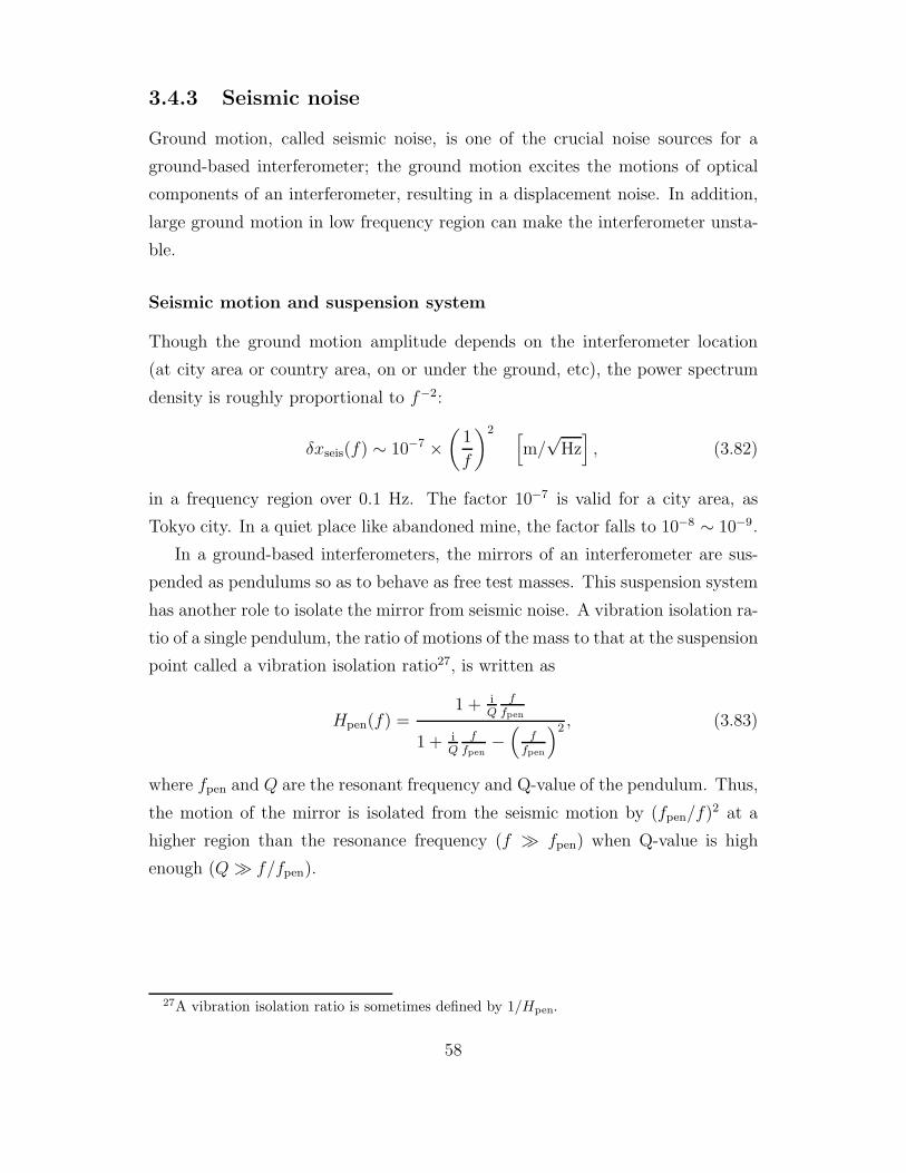
3.4.3 Seismic noise
Ground motion, called seismic noise, is one of the crucial noise sources for a
ground-based interferometer; the ground motion excites the motions of optical
components of an interferometer, resulting in a displacement noise. In addition,
large ground motion in low frequency region can make the interferometer unsta-
ble.
Seismic motion and suspension system
Though the ground motion amplitude depends on the interferometer location
(at city area or country area, on or under the ground, etc), the power spectrum
density is roughly proportional to f−2:
δxseis(f) ∼ 10−7 ×(
1
f
)2 [m/
√Hz], (3.82)
in a frequency region over 0.1 Hz. The factor 10−7 is valid for a city area, as
Tokyo city. In a quiet place like abandoned mine, the factor falls to 10−8 ∼ 10−9.
In a ground-based interferometers, the mirrors of an interferometer are sus-
pended as pendulums so as to behave as free test masses. This suspension system
has another role to isolate the mirror from seismic noise. A vibration isolation ra-
tio of a single pendulum, the ratio of motions of the mass to that at the suspension
point called a vibration isolation ratio27, is written as
Hpen(f) =1 + i
Qf
fpen
1 + iQ
ffpen
−(
ffpen
)2 , (3.83)
where fpen and Q are the resonant frequency and Q-value of the pendulum. Thus,
the motion of the mirror is isolated from the seismic motion by (fpen/f)2 at a
higher region than the resonance frequency (f fpen) when Q-value is high
enough (Q f/fpen).
27A vibration isolation ratio is sometimes defined by 1/Hpen.
58

Vibration isolation system
In practice, the seismic isolation ratio of a simple single pendulum is not sufficient
for the detection of gravitational waves28. Since the resonant frequency, fpen, is
around 1 Hz in a single pendulum with a reasonable length (a few tens of cm),
the vibration isolation ratio is about 10−4 at 100 Hz. In a typical design of
an interferometer, the vibration isolation ratio is required over 10−8 ∼ 10−9 at
100 Hz. In order to realize such a high vibration isolation ratio, several design
of the isolation system is proposed: a multi-stage pendulum, a low-resonant-
frequency pendulum, combination of other isolation systems like a stack system.
In a n-stage pendulum, the vibration isolation ratio is expressed roughly29 as
Hn−pen = (fpen/f)2n. On the other hand, the vibration isolation ratio is improved
by a low-resonant-frequency pendulum as implied in Eq. (3.83); it is proportional
to f2pen. A low-resonant-frequency pendulum is realized with a reasonable size
by X-pendulum [61, 62], and active controlled pendulum. The seismic vibration
is also isolated with a stack system. A stack is composed of multi-layers of soft
rubber and dense mass, as biton and stainless.
Stable operation against a ground motion
A ground motion affects not only the sensitivity of the interferometer, but also the
stability of it. Though the suspension system and other isolation system isolate
the mirror from seismic motion in a high frequency region as described above, the
mirror motion is largely excited in a low frequency region, especially at the reso-
nant frequency of the pendulum. When the Q-value is high enough, the transfer
function described by Eq. (3.83) is approximated as H(ωpen) ∼ Q. The large
motion at the resonant frequency of the pendulum can disturb the operational
condition of an interferometer, which affects the stability of the operation, and
also the sensitivity of the interferometer. In addition to the longitudinal motion,
the rotational motions of the mirrors are also excited at the resonant frequency,
28In this part, we concentrate on the vibration isolation for a displacement, the length degree
of freedom, of an interferometer. However, in practice, the vertical and orientation vibrations of
the mirrors cause a displacement noise coupling with the asymmetries of the isolation system,
differences of the gravity direction in mirrors, and miss centering of the laser beam.29In practice, the vibration isolation ratio is degraded by various resonances.
59
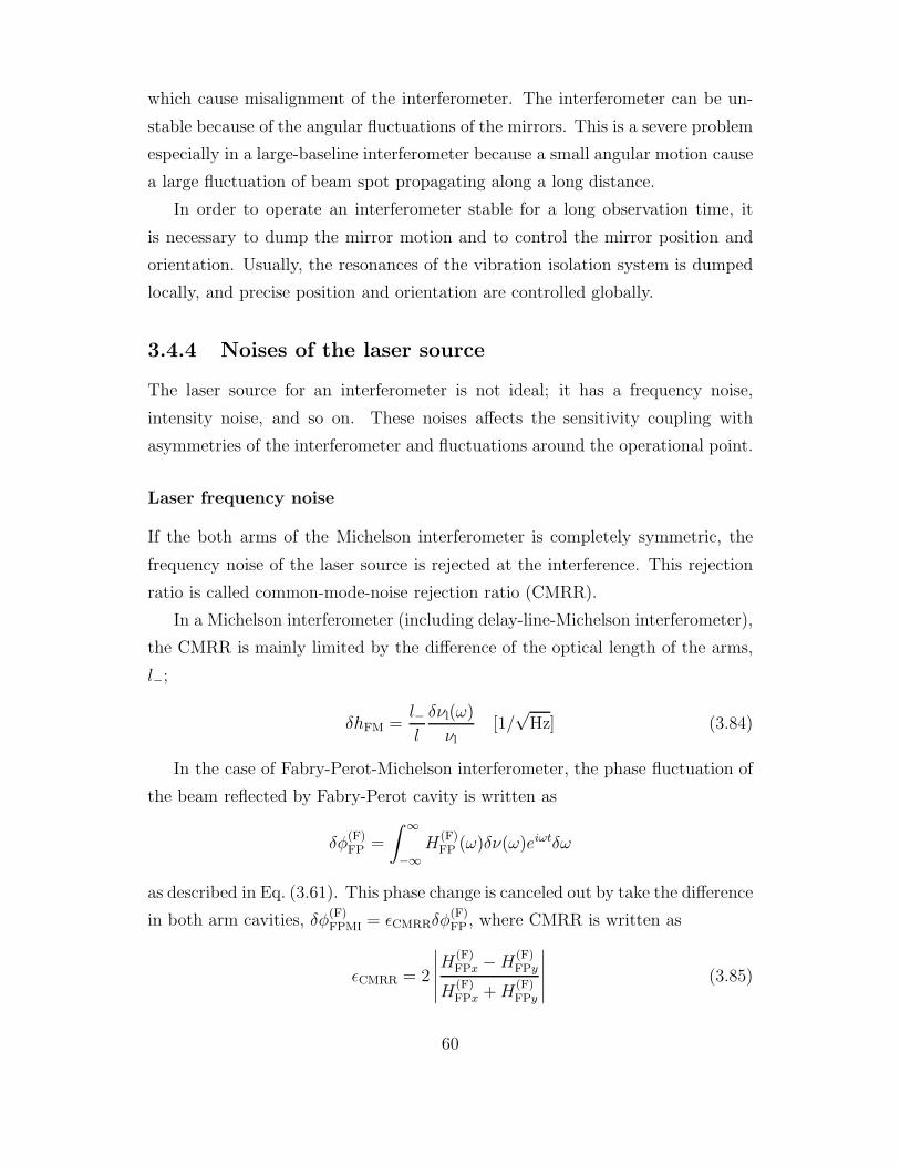
which cause misalignment of the interferometer. The interferometer can be un-
stable because of the angular fluctuations of the mirrors. This is a severe problem
especially in a large-baseline interferometer because a small angular motion cause
a large fluctuation of beam spot propagating along a long distance.
In order to operate an interferometer stable for a long observation time, it
is necessary to dump the mirror motion and to control the mirror position and
orientation. Usually, the resonances of the vibration isolation system is dumped
locally, and precise position and orientation are controlled globally.
3.4.4 Noises of the laser source
The laser source for an interferometer is not ideal; it has a frequency noise,
intensity noise, and so on. These noises affects the sensitivity coupling with
asymmetries of the interferometer and fluctuations around the operational point.
Laser frequency noise
If the both arms of the Michelson interferometer is completely symmetric, the
frequency noise of the laser source is rejected at the interference. This rejection
ratio is called common-mode-noise rejection ratio (CMRR).
In a Michelson interferometer (including delay-line-Michelson interferometer),
the CMRR is mainly limited by the difference of the optical length of the arms,
l−;
δhFM =l−l
δνl(ω)
νl
[1/√
Hz] (3.84)
In the case of Fabry-Perot-Michelson interferometer, the phase fluctuation of
the beam reflected by Fabry-Perot cavity is written as
δφ(F)FP =
∫ ∞
−∞H
(F)FP (ω)δν(ω)eiωtδω
as described in Eq. (3.61). This phase change is canceled out by take the difference
in both arm cavities, δφ(F)FPMI = εCMRRδφ
(F)FP , where CMRR is written as
εCMRR = 2
∣∣∣∣∣H(F)FPx − H
(F)FPy
H(F)FPx + H
(F)FPy
∣∣∣∣∣ (3.85)
60

With approximations rE ' 1 and ω ωc, εCMRR is written as
εCMRR ∼ L−L
+F−F . (3.86)
This equation shows that the CMRR is limited by the difference of the arm length
and finesse, in other words, by the difference of total optical path length.
By using high-quality optical components, it is believed that a CMRR of
1/100 is achievable. So far, a CMRR of 1/300 is experimentally realized with a
prototype interferometer [31].
Even if an interferometer has a good CMRR of 1/100, the frequency fluctu-
ation is still a large noise source for the detection of gravitational waves. Thus,
the laser frequency is stabilized using cavities: a rigid cavity with a length about
a few tens of cm, a independently suspended cavity like mode cleaner, and the
arm cavity of the interferometer itself.
Laser intensity noise
A Michelson interferometer converts a phase information of the laser beam to a
intensity change at the photo detector. Thus, it is necessary to exclude the effect
of intensity fluctuation from the signal port. By setting the operational point to
dark fringe, the effect of intensity noise is reduced. In addition, in a modulation
scheme, the modulation frequency is usually selected to be over 10 MHz, in which
the intensity noise of the laser source is smaller than the shot noise.
However, in practice, there remains a fluctuation around the dark point be-
cause of a finite control gain. The residual motion around the fringe couples with
the intensity noise of the laser source30:
δxint =δP
Pδxrms [m/
√Hz], (3.87)
where δxrms is the residual RMS (root mean square) fluctuation around the dark
fringe. Thus, the control gain have to be large enough to suppress the residual
RMS deviation, as well as the intensity stabilization of the laser source.
30In a power-recycled interferometer, the intensity noise includes the fluctuation of the recy-
cling gain.
61

Laser mode noise
The fluctuations of the orientation (called beam jitter) and radius of the laser
source can be a noise source coupling with misalignment of the interferometer or
inhomogeneity of the photo detector [63, 64]. These fluctuations are interpreted
to be a fluctuation of the mode of the laser source: the beam orientation error
is the mixing of the first-order (and higher) Hermite-Gaussian modes, the beam
radius error is the mixing of the second-order (and higher) Hermite-Gaussian
modes.
These higher-mode beams are usually rejected by a mode cleaner placed be-
tween the laser source and the interferometer. Mode cleaner is, in principle, a
Fabry-Perot cavity formed by two mirrors with same and high reflectivity, which
has a high finesse and transmissivity31. The mode cleaner is set to resonate with
the TEM00 mode beam, and not to resonate with the higher-mode beams. In
this condition, only TEM00 mode beam transmits through the mode cleaner and
higher-mode beam is reflected back. In order to reduce the effect of the seismic
noise, the mode cleaner has a long baseline, and its mirrors are suspended to
isolate from the seismic motion [65, 66, 67].
3.4.5 Residual gas noise
The fluctuation of the gas along the optical pass cause a fluctuation of a reflective
index, resulting in the change in optical pass length. Thus, the interferometer is
housed in a vacuum system32. The residual noise level is written as [68]
δhrg =
[4√
2π
L
(n0 − 1)2
(A0/V0)u0
√Lλl
(p
p0
)(T0
T
)3/2]1/2
[1/√
Hz], (3.88)
31A ring-type cavity comprised of three or four mirrors is often used as a mode cleaner.
Compared with ring-type, a mode cleaner formed by two mirrors are called linear-type mode
cleaner. In principle, there is little difference between a ring-type and linear-type as long as the
angle of the the incident and reflected beams on the mirror is small enough. However, a ring-
type cavity has an advantage that the main interferometer is less affected by the back-scattered
light from the mode cleaner.32The vacuum system has other roles: to avoid a loss of laser power by the absorption and
scattering of the gas, to keep the optical components from shaken by a fluctuation of gas, and
from the contamination of the optics by dusts.
62

where A0: Avogadro’s number33, V0: volume of one mole gas at standard tem-
perature (T0) and pressure (p0)34, n0: reflective index of the gas, and u0: mean
velocity of the gas molecule at standard state. In order to reduce this level to
10−24 1/√
Hz with a 3 km baseline length, the pressure of 10−6 Pa is required.
3.4.6 Noises due to control of the interferometer
In order to operate an interferometric gravitational wave detector, it is necessary
to control the position of the optical components. However, the control system
can introduce noises without a proper design. Though this is not a fundamental
noise, careful consideration and design are required to avoid this noise in practice.
Noises due to the control loops
In case of Fabry-Perot-type interferometer, if the arm cavities are controlled to
resonate with the incident laser beam independently, the control system also
suppresses the gravitational wave signal, resulting in the increase of noise level.
This affect is avoided by narrowing the control frequency band for the arm mirrors
than the observation band (called loose lock). However, with a narrow control
band, the fluctuation of the interferometer remain because of a low control gain.
This residual fluctuation cause additional noises. Moreover the interferometer will
not be operated stably for a long observation time with a narrow control band.
Thus, the arm mirrors must be controlled using the differential motion signal of
arms, i.e., the signal for a gravitational wave. In this case, the interferometer can
be operated with wide frequency band (called tight lock) without suppressing the
signal of gravitational waves. The gravitational wave signal is obtained from the
feedback signal to the mirrors.
Besides the differential motion of the arms, the other degrees of freedom must
be controlled with auxiliary control loops. However, in general, S/N (signal-to-
noise ratio) of the signal for these control is not as good as that for the main
control loop. Thus, the control loops must be designed so that the optical com-
ponents would not be shaken by feeding back worse S/N signals. In most cases,
33Avogadro’s number: A0 = 6.02 × 1023.34Volume of one mole gas at standard state: V0 = 22.4 × 10⁻³ [m3/mol].
63

the control bandwidth of the auxiliary control loops must be much narrower than
the observation frequency band.
Actuator noise and dynamic range
The mirror actuator driver also has an electronic noise. Since the driver noise
shakes a mirror directly, it should be designed to have extremely low noise. The
driver noise is reduced by decreasing the efficiency of the actuator. However, in
this case, the dynamic range of the actuator is also reduced. Since the actuator
must have sufficient dynamic range to compensate the motion of the interferom-
eter, the efficiency of the actuator is optimized considering the driver noise and
the required dynamic range. A multi-stage actuator, the combination of a high-
dynamic-range actuator and a low-noise actuator will be useful if one actuator
does not satisfy the noise level and dynamic range simultaneously.
64

Chapter 4
Signal separation scheme
In this Chapter, we describe the signal extraction and control scheme of a power-
recycled Fabry-Perot-Michelson interferometer.
To behave as a free mass, each mirror of an interferometric gravitational wave
detector is suspended as pendulum. Though the suspension system has another
role to isolate the mirror from the seismic motion at the observation frequency
band, the mirror is largely excited by the the seismic motion at the resonant
frequency of the pendulum. Thus, it is necessary to control an interferometer
and keep it at the operational point. The signals necessary for control of a
power-recycled Fabry-Perot-Michelson interferometer is extracted with a scheme
called frontal modulation. However, the control signal for the recycling cavity
length cannot be separated independently of other signals.
In order to solve this signal mixing problem, we have invented a new scheme
to separate the control signals by an adjustment of the optical parameters of the
interferometer. One of the advantage of this scheme is that this scheme does not
require any additional optical components nor modulation to separate signals.
In the first half of this Chapter, we describe the signal-extraction scheme
with frontal modulation, which is the basis of our signal-separation scheme. The
principle of the signal-separation scheme is described in the latter half of this
Chapter. This Chapter contains the following Sections.
• Overview of the control system. The overview of the signal-extraction
and control scheme of a power-recycled Fabry-Perot-Michelson interferom-
eter.
65

Front mirror
End mirror
Front mirror End mirror
Fabry-Perot arm cavities
Recycling mirrorLaser source
Lx
Photo detector
Gravitational wave signal
Beam splitter
lx
ly
Ly
Figure 4.1: Power recycled Fabry-Perot-Michelson interferometer. Four
degrees of freedom must be controlled to operate the interferometer.
• Frontal modulation. Modulation and demodulation for signal extraction.
Response of the interferometer.
• Signal sensitivity. Sensitivities of the signals expected with frontal mod-
ulation under operational conditions.
• Signal-separation scheme. The signal-separation scheme with adjust-
ment of optical parameters.
4.1 Overview of control schemes
4.1.1 Power-recycled Fabry-Perot-Michelson interferome-
ter
Figure. 4.1 shows the optical configuration of a Fabry-Perot-Michelson interfer-
ometer with power recycling. To operate this interferometer, four degrees of
longitudinal freedom must be controlled: the lengths of the arm cavities (δLx
and δLy), the lengths between the recycling mirror and the front mirrors (δlx and
δly). The operational point is selected so that the interferometer would be oper-
66
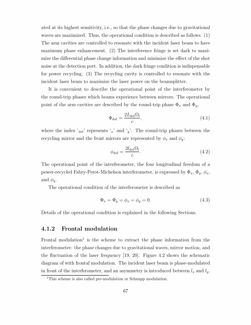
ated at its highest sensitivity, i.e., so that the phase changes due to gravitational
waves are maximized. Thus, the operational condition is described as follows. (1)
The arm cavities are controlled to resonate with the incident laser beam to have
maximum phase enhancement. (2) The interference fringe is set dark to maxi-
mize the differential phase change information and minimize the effect of the shot
noise at the detection port. In addition, the dark fringe condition is indispensable
for power recycling. (3) The recycling cavity is controlled to resonate with the
incident laser beam to maximize the laser power on the beamsplitter.
It is convenient to describe the operational point of the interferometer by
the round-trip phases which beams experience between mirrors. The operational
point of the arm cavities are described by the round-trip phase Φx and Φy,
Φdof =2LdofΩl
c, (4.1)
where the index ‘dof’ represents ‘x’ and ‘y’. The round-trip phases between the
recycling mirror and the front mirrors are represented by φx and φy:
φdof =2ldofΩl
c. (4.2)
The operational point of the interferometer, the four longitudinal freedom of a
power-recycled Fabry-Perot-Michelson interferometer, is expressed by Φx, Φy, φx,
and φy.
The operational condition of the interferometer is described as
Φx = Φy = φx = φy = 0. (4.3)
Details of the operational condition is explained in the following Sections.
4.1.2 Frontal modulation
Frontal modulation1 is the scheme to extract the phase information from the
interferometer: the phase changes due to gravitational waves, mirror motion, and
the fluctuation of the laser frequency [19, 20]. Figure 4.2 shows the schematic
diagram of with frontal modulation. The incident laser beam is phase-modulated
in front of the interferometer, and an asymmetry is introduced between lx and ly.
1This scheme is also called pre-modulation or Schnupp modulation.
67
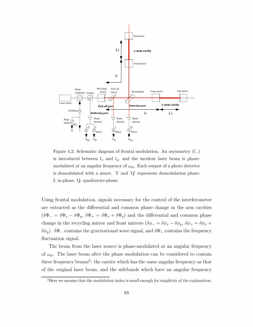
Front mirror
Front mirror
End mirror
End mirrorBeamsplitterPick-offmirror
Recycling mirror
Laser source
Phasemodulator Isolator
Detection portPick-off port
Reflection port
Photodetector
Photodetector
Photodetector
x-arm cavity
Oscillator
Q I I
VPI
QQ I
π/2
VDQVRIVRQ
MixerMixerMixer
Phaseshifter
Ly y-arm cavity
Lxlx
ly
Figure 4.2: Schematic diagram of frontal modulation. An asymmetry (l−)
is introduced between lx and ly, and the incident laser beam is phase-
modulated at an angular frequency of ωm. Each output of a photo detector
is demodulated with a mixer. ’I’ and ’Q’ represents demodulation phase:
I: in-phase, Q: quadrature-phase.
Using frontal modulation, signals necessary for the control of the interferometer
are extracted as the differential and common phase change in the arm cavities
(δΦ− = δΦx − δΦy, δΦ+ = δΦx + δΦy) and the differential and common phase
change in the recycling mirror and front mirrors (δφ− = δφx − δφy, δφ+ = δφx +
δφy). δΦ− contains the gravitational wave signal, and δΦ+ contains the frequency
fluctuation signal.
The beam from the laser source is phase-modulated at an angular frequency
of ωm. The laser beam after the phase modulation can be considered to contain
three frequency beams2: the carrier which has the same angular frequency as that
of the original laser beam, and the sidebands which have an angular frequency
2Here we assume that the modulation index is small enough for simplicity of the explanation.
68
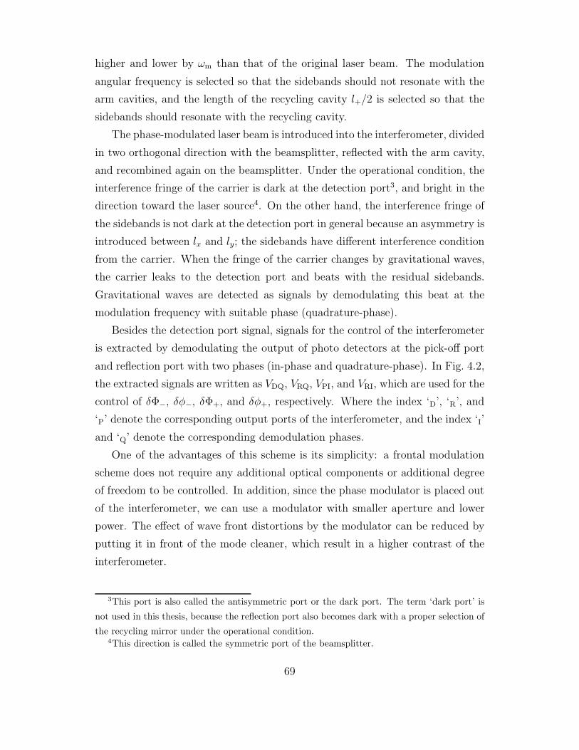
higher and lower by ωm than that of the original laser beam. The modulation
angular frequency is selected so that the sidebands should not resonate with the
arm cavities, and the length of the recycling cavity l+/2 is selected so that the
sidebands should resonate with the recycling cavity.
The phase-modulated laser beam is introduced into the interferometer, divided
in two orthogonal direction with the beamsplitter, reflected with the arm cavity,
and recombined again on the beamsplitter. Under the operational condition, the
interference fringe of the carrier is dark at the detection port3, and bright in the
direction toward the laser source4. On the other hand, the interference fringe of
the sidebands is not dark at the detection port in general because an asymmetry is
introduced between lx and ly; the sidebands have different interference condition
from the carrier. When the fringe of the carrier changes by gravitational waves,
the carrier leaks to the detection port and beats with the residual sidebands.
Gravitational waves are detected as signals by demodulating this beat at the
modulation frequency with suitable phase (quadrature-phase).
Besides the detection port signal, signals for the control of the interferometer
is extracted by demodulating the output of photo detectors at the pick-off port
and reflection port with two phases (in-phase and quadrature-phase). In Fig. 4.2,
the extracted signals are written as VDQ, VRQ, VPI, and VRI, which are used for the
control of δΦ−, δφ−, δΦ+, and δφ+, respectively. Where the index ‘D’, ‘R’, and
‘P’ denote the corresponding output ports of the interferometer, and the index ‘I’
and ‘Q’ denote the corresponding demodulation phases.
One of the advantages of this scheme is its simplicity: a frontal modulation
scheme does not require any additional optical components or additional degree
of freedom to be controlled. In addition, since the phase modulator is placed out
of the interferometer, we can use a modulator with smaller aperture and lower
power. The effect of wave front distortions by the modulator can be reduced by
putting it in front of the mode cleaner, which result in a higher contrast of the
interferometer.
3This port is also called the antisymmetric port or the dark port. The term ‘dark port’ is
not used in this thesis, because the reflection port also becomes dark with a proper selection of
the recycling mirror under the operational condition.4This direction is called the symmetric port of the beamsplitter.
69
4.1.3 Signal separation
As described above, all of the signals necessary for the longitudinal control
of a power-recycled Fabry-Perot-Michelson interferometer are extracted using a
frontal modulation scheme. However, there is a difficulty in extracting the signal
for the control of the recycling cavity length (δφ+) independently; this signal is
mixed with the large δΦ+ signal5. The mixing among the signals complicates the
design of the control system which maintains the stability and high sensitivity
at the same time [19]. It is therefore desirable to obtain well-separated signals.
Such signals would simplify the design and study of the control system, and the
operation of the interferometer. Some methods to obtain such signals have been
proposed or tested.
One method to separate signals is to combine the signals linearly by electronic
circuits (the decoding circuits) or by digital processing [19, 20, 69, 70]. Though
the four signals are extracted separately by this linear-combination operation, the
signal-to-noise ratios of these signals can decrease with a proper design because
the noises, such as the shot noise, are also combined.
The other method to separate signals is to use an additional carrier, called
a subcarrier [21, 22, 70]. The frequency of the subcarrier is offset from that of
the main carrier. The frequency-shifted subcarrier is superimposed on the main
carrier with a beamsplitter after phase modulation. The frequency offset and
the modulation frequency for the subcarrier are selected so that the subcarrier
and its RF sidebands do not resonate with the arm cavities, but resonate with
the recycling cavity. Using a frequency-shifted subcarrier, the information about
the power-recycled Michelson part of the interferometer (δφ− and δφ+) is ob-
tained independently of δΦ− and δΦ+ because the subcarrier and its sidebands
are unaffected by the phase changes in the arm cavities. However, this method
complicates the optical setup for introduction of the subcarrier.
The scheme described in this thesis is a signal-separation technique by adjust-
ing the optical parameters of the interferometer [33]. The point of this method
is to adjust the reflectivity of the recycling mirror so as to maximize the gain of
5This problem is not a characteristic one with frontal modulation. The phase change of the
carrier is much more sensitive to δΦ+ than δφ+ at the bright fringe of the interference. This is
because δΦ+ information is enhanced in the arm cavities.
70

Photodetector
EPD = xEinc
Mixer Filter Signal
I or Q
Phasemodulator
Interferometer
Laser source
EincOscillator
Q I
π/2
Phaseshifter
Figure 4.3: Signal extraction scheme using modulation and demodulation.
The interferometer is regarded as a black box which causes amplitude and
phase change onto the incident laser beams.
the sidebands, not the gain of the carrier. By this modification of the optical
parameters, the signals are extracted separately at only a little expense of the
recycling gain. This scheme does not call for any additional optics or electronic
components to extract the δl+ signal, and maintains the advantage of simplicity
with a frontal modulation technique.
4.2 Frontal modulation
In this Section, the general expressions of the signals extracted with frontal mod-
ulation are described. In frontal modulation, it is possible to consider the mod-
ulation system and the interferometer separately. The signal extraction system
with modulation and demodulation is described in the first half of this Section,
and the response of the interferometer is described in the latter half.
4.2.1 Modulation and demodulation
A laser-interferometric gravitational wave detector is a device to detect the phase
change of the laser beam caused by gravitational waves. However, the phase of the
laser beam is not detected directly with a photo detector, because the frequency
71

of the laser beam is much higher than the response speed of a photo diode6. A
photo diode detects the power of the laser beam averaged during the response
time scale. The phase information of the laser beam is lost in the averaging
process.
Thus, the phase modulation scheme is used to detect the phase change in
the laser beam7. Figure 4.3 shows the diagram of the phase detection scheme
using modulation and demodulation. In a frontal modulation technique, the laser
beam from the laser source is phase-modulated in front of the interferometer. The
phase-modulated beam is considered as the super position of monochromatic laser
beams: a carrier and sidebands. The carrier has the same frequency as that of
the original laser beam. On the other hand, the frequency of the sidebands are
shifted by integral multiples of the modulation frequency. The laser beam is
detected with the photo detector after experiencing amplitude and phase change
in the interferometer. The amplitude and phase change in the interferometer is
detected by demodulating the output of the photo detector.
Phase modulation
The laser beam from the laser source is expressed as
El = E0eiΩlt, (4.4)
where E0 is the amplitude of the laser beam. In this thesis, amplitudes of laser
beam are normalized to have a unit of√
W. Thus the output power of the laser
source is written as
Pl = |El|2 [W]. (4.5)
This laser beam is introduced into the interferometer after phase modulation
at an angular frequency of ωm and a modulation index of mm. The modulation
6The frequency of a Nd:YAG laser (infrared) is about 300 THz. The response speed of a
photo diode is about 100 MHz at best.7The phase change in the laser beam can be detected without phase modulation by proper
selection of the operational point. The Michelson interferometer converts the phase change to
the power change in the interference fringe as described in Eq. (3.2). This phase detection
scheme is called DC-scheme or differential scheme. Though the differential scheme is simple
and convenient, it is incompatible with power recycling.
72
Frequency
Carrier
Sideband
Ωl Ω l+ωmΩ l-ωmΩ l-2ωm Ω l+2ωm Ω l+3ωmΩ l-3ωm
|Amplitude|
Figure 4.4: Phase modulated laser beam is considered to be the superpo-
sition of monochromatic beams; the angular frequencies are separated by
the modulation frequency (ωm/2π). The laser beam which has the same
frequency as that of the original laser beam is called carrier, and the laser
beam generated by the modulation is called sidebands.
frequency is usually selected to be a few tens of megahertz in order to avoid the
intensity noise of the laser source. The incident laser beam into the interferometer
is written as
Einc = Eleimm cos ωmt. (4.6)
Here, Eq. (4.6) is rewritten using Bessel functions Jn as8
Einc = El
∞∑n=−∞
inJneinωmt (4.7)
= E0
∞∑n=−∞
inJne
i(Ωl+nωm)t
. (4.8)
8The exponential part is expanded as
eimm cos ωmt =∞∑
n=−∞inJneinωmt.
Bessel functions satisfy the following expressions:
J−n = (−1)nJn
Jn ' 1n!
(mm
2
)n
(mm 1).
The Bessel functions Jn(mm) are written as Jn for simplicity of expressions in this thesis.
73
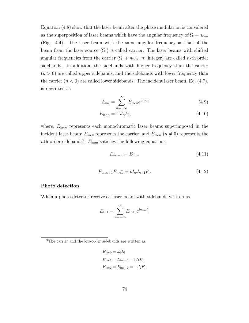
Equation (4.8) show that the laser beam after the phase modulation is considered
as the superposition of laser beams which have the angular frequency of Ωl +nωm
(Fig. 4.4). The laser beam with the same angular frequency as that of the
beam from the laser source (Ωl) is called carrier. The laser beams with shifted
angular frequencies from the carrier (Ωl + nωm, n: integer) are called n-th order
sidebands. In addition, the sidebands with higher frequency than the carrier
(n > 0) are called upper sidebands, and the sidebands with lower frequency than
the carrier (n < 0) are called lower sidebands. The incident laser beam, Eq. (4.7),
is rewritten as
Einc =∞∑
n=−∞Eincne
inωmt (4.9)
Eincn = inJnEl, (4.10)
where, Eincn represents each monochromatic laser beams superimposed in the
incident laser beam; Einc0 represents the carrier, and Eincn (n 6= 0) represents the
nth-order sidebands9. Eincn satisfies the following equations:
Einc−n = Eincn (4.11)
Eincn+1Einc∗n = iJnJn+1Pl. (4.12)
Photo detection
When a photo detector receives a laser beam with sidebands written as
EPD =
∞∑n=−∞
EPDneinωmt,
9The carrier and the low-order sidebands are written as
Einc0 = J0El
Einc1 = Einc−1 = iJ1El
Einc2 = Einc−2 = −J2El,
74

the photo current caused by the input beam is written as
IPD = η|EPD|2 = η
[ ∞∑n=−∞
∞∑m=−∞
EPDmEPD∗m−ne
inωmt
]
=∞∑
n=−∞IPDneinωmt [A], (4.13)
where η [A/W] is the photo efficiency of the photo diode. IPDn represents the
photo current at the angular frequency of nωm:
IPDn = η
∞∑m=−∞
EPDmEPD∗m−n. (4.14)
Equation (4.13) shows that the photo current contain DC photo current and
integer multiple element of the modulation frequency. The photo current at the
modulation frequency (n = 1) is written as10
IPD1 = η∞∑
m=0
[EPDm+1EPD
∗m + EPD−mEPD
∗−m−1
]. (4.15)
Demodulation
The modulation frequency element of the photo current (IPD1) is extracted by
demodulating the the output of the photo diode at the angular frequency of ωm.
The demodulation is realized with a mixer and a low pass filter. The mixer down-
converts the ωm elements of the photo current to the frequency region near DC
by multiplying the output of the photo diode and local oscillator which has the
angular frequency of ωm. The low pass filter rejects the higher frequency elements
over ωm from the output of the mixer.
Two independent outputs are obtained by the demodulation depending on
the phase of the local oscillator: in-phase and quadrature-phase. The output of
10IPDn satisfies the equation
IPD−n = IPD∗n.
75

the demodulator is described as
VPDI =gdet
T
∫ t
t−T
IPD(t′) cos ωmt′dt′
=gdet
2(IPD1 + IPD−1) = gdetReIPD1
= gdetη
∞∑n=0
ReEPDn+1EPD
∗n + EPD−nEPD
∗−n−1
, (4.16)
when cos ωmt (in-phase) is used as the local oscillator. The gain of the photo
detector and the efficiency of the demodulator are represented by the coefficient
gdet [Ω]. On the other hand, when sin ωmt (quadrature-phase) is used as the local
oscillator, the output of the demodulator is written as
VPDQ =gdet
T
∫ t
t−T
IPD(t′) sinωmt′dt′
=gdet
2i(−IPD1 + IPD−1) = −gdetImIPD1
= −gdetη∞∑
n=0
ImEPDn+1EPD
∗n + EPD−nEPD
∗−n−1
. (4.17)
Equations (4.16) and (4.17) show that the real and imaginary part of IPD1 are
extracted depending on the phase of the local oscillator11.
Signal corresponding to the response of the interferometer
The phase-modulated laser beam Einc is detected with the photo detector af-
ter experiencing amplitude and phase change in the interferometer. The each
frequency element of the input laser beam on the photo detector is written as
EPDn = xnEincn, (4.18)
11In general, since the local oscillator with the phase of θm is written as
cos(ωmt + θm) = cos ωmt cos θm − sin ωmt sin θm,
the output of the demodulator is written as the linear combination of the in-phase and
quadrature-phase outputs:
VPDθm =gdet
T
∫ t
t−T
IPD(t′) cos(ωmt′ + θm)dt′
= VPDI cos θm − VPDQ sin θm.
76
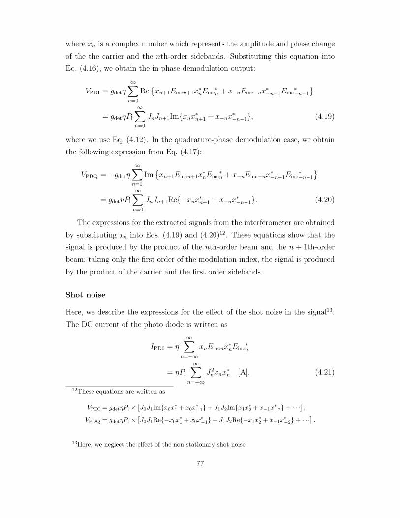
where xn is a complex number which represents the amplitude and phase change
of the the carrier and the nth-order sidebands. Substituting this equation into
Eq. (4.16), we obtain the in-phase demodulation output:
VPDI = gdetη∞∑
n=0
Rexn+1Eincn+1x
∗nEinc
∗n + x−nEinc−nx
∗−n−1Einc
∗−n−1
= gdetηPl
∞∑n=0
JnJn+1Imxnx∗n+1 + x−nx
∗−n−1, (4.19)
where we use Eq. (4.12). In the quadrature-phase demodulation case, we obtain
the following expression from Eq. (4.17):
VPDQ = −gdetη
∞∑n=0
Imxn+1Eincn+1x
∗nEinc
∗n + x−nEinc−nx∗
−n−1Einc∗−n−1
= gdetηPl
∞∑n=0
JnJn+1Re−xnx∗n+1 + x−nx∗
−n−1. (4.20)
The expressions for the extracted signals from the interferometer are obtained
by substituting xn into Eqs. (4.19) and (4.20)12. These equations show that the
signal is produced by the product of the nth-order beam and the n + 1th-order
beam; taking only the first order of the modulation index, the signal is produced
by the product of the carrier and the first order sidebands.
Shot noise
Here, we describe the expressions for the effect of the shot noise in the signal13.
The DC current of the photo diode is written as
IPD0 = η∞∑
n=−∞xnEincnx∗
nEinc∗n
= ηPl
∞∑n=−∞
J2nxnx∗
n [A]. (4.21)
12These equations are written as
VPDI = gdetηPl ×[J0J1Imx0x
∗1 + x0x
∗−1 + J1J2Imx1x
∗2 + x−1x
∗−2 + · · ·] ,
VPDQ = gdetηPl ×[J0J1Re−x0x
∗1 + x0x
∗−1 + J1J2Re−x1x
∗2 + x−1x
∗−2 + · · ·] .
13Here, we neglect the effect of the non-stationary shot noise.
77

The shot noise is written as
IPDshotn =√
2eIPD0 [A/√
Hz]. (4.22)
Since the eiωmt element (IPDshot1) and the e−iωmt element (IPDshot−1) of the photo
current caused by the shot noise have no correlation, the effect of the shot noise
in the output of the demodulator is written as
VPDshot =gdet
2
√I2PDshot1 + I2
PDshot−1 = gdet
√eIPD0 [V/
√Hz]. (4.23)
Sensitivity of the signal
The sensitivity of a signal is represented by the change in the signal corresponding
to the change in the interferometer. When the change in the interferometer is
small enough, the signal is considered to have a linear response:
δVPDdem =∂VPDdem
∂θδθ, (4.24)
where θ represents the phase (Φ−, φ−, Φ+, and φ+), and index ‘dem’ represents
the demodulation phase (‘I’ or ‘Q’). In this equation, the derivative ∂VPDdem/∂θ
represents the sensitivity of the signal VPDdem to the degree of freedom θ. From
Eqs. (4.19) and (4.20), the sensitivity of the signal is written as
∂VPDI
∂θ= gdetηPl
∞∑n=0
JnJn+1 ×
Im
xn
∂x∗n+1
∂θ+ x−n
∂x∗−n−1
∂θ+
∂xn
∂θx∗
n+1 +∂x−n
∂θx∗−n−1
(4.25)
∂VPDQ
∂θ= gdetηPl
∞∑n=0
JnJn+1 ×
Re
−xn
∂x∗n+1
∂θ+ x−n
∂x∗−n−1
∂θ− ∂xn
∂θx∗
n+1 +∂x−n
∂θx∗−n−1
(4.26)
The sensitivity of the signal limited by the shot noise (the shot-noise level) is
written as the ratio of the shot noise and the sensitivity of the signal:
θshot =VPDshot(∂VPDdem
∂θ
) . (4.27)
78
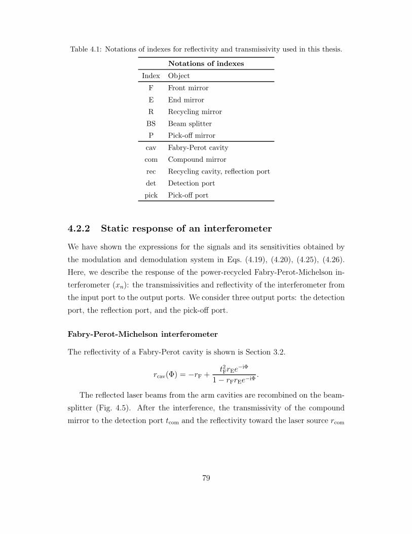
Table 4.1: Notations of indexes for reflectivity and transmissivity used in this thesis.
Notations of indexes
Index Object
F Front mirror
E End mirror
R Recycling mirror
BS Beam splitter
P Pick-off mirror
cav Fabry-Perot cavity
com Compound mirror
rec Recycling cavity, reflection port
det Detection port
pick Pick-off port
4.2.2 Static response of an interferometer
We have shown the expressions for the signals and its sensitivities obtained by
the modulation and demodulation system in Eqs. (4.19), (4.20), (4.25), (4.26).
Here, we describe the response of the power-recycled Fabry-Perot-Michelson in-
terferometer (xn): the transmissivities and reflectivity of the interferometer from
the input port to the output ports. We consider three output ports: the detection
port, the reflection port, and the pick-off port.
Fabry-Perot-Michelson interferometer
The reflectivity of a Fabry-Perot cavity is shown is Section 3.2.
rcav(Φ) = −rF +t2FrEe−iΦ
1 − rFrEe−iΦ.
The reflected laser beams from the arm cavities are recombined on the beam-
splitter (Fig. 4.5). After the interference, the transmissivity of the compound
mirror to the detection port tcom and the reflectivity toward the laser source rcom
79

y-arm cavity
Beamsplitter
Pick-off mirror
E BSE eff
E cir
E PO E anti
E sym
x-arm cavity
Figure 4.5: Field around the beamsplitter of Fabry-Perot-Michelson inter-
ferometer. The beam going upward of this figure from the pick-off mirror
and the transmitted beams through the cavities are not drawn.
are written as14
rcom(θop) =Ecir
Eeff= t2P
t2BSrcavx(Φx)e
−iφx + r2BSrcavy(Φy)e
−iφy
(4.28)
tcom(θop) =Eanti
Eeff= tBSrBStP
rcavx(Φx)e
−iφx − rcavy(Φy)e−iφy
, (4.29)
where indexes ‘BS’ and ‘P’ denote the beamsplitter and the pick-off mirror, re-
spectively. θop represents the operational point of the interferometer, the function
of Φx, Φy, φx, and φy (or Φ−, φ−, Φ+, and φ+).
Here, Eq. (4.28) is rewritten using the sum and difference of φ+ and φ− as
rcom(θop) = e−iφ+2
rcom+ cos
(φ−2
)− ircom− sin
(φ−2
), (4.30)
where rcom+ and rcom− correspond to the sum and difference of two arms:
rcom+ = t2Pt2BSrcavx(Φx) + r2
BSrcavy(Φy)
(4.31)
rcom− = t2Pt2BSrcavx(Φx) − r2
BSrcavy(Φy)
. (4.32)
If both arm is completely symmetric, rcom− = 0.
Same as rcom, tcom in Eq. (4.29) is rewritten as
tcom(θop) = e−iφ+2
tcom− cos
(φ−2
)− itcom+ sin
(φ−2
). (4.33)
14In the calculation, we consider that the recycling mirror, the pick-off mirror, and the beam-
splitter are placed close to one another, and that the photo detectors at the output ports of the
interferometer are placed at the same distance from the interferometer.
80

Where tcom+ and tcom− correspond to the sum and difference of two arms:
tcom+ = tBSrBStP rcavx(Φx) + rcavy(Φy) (4.34)
tcom− = tBSrBStP rcavx(Φx) − rcavy(Φy) . (4.35)
The compound mirror also transmits the input laser beam to the pick-off port.
This transmissivity tcomP is
tcomP(θop) =rP
tPrcom. (4.36)
Recycling cavity
The response of the recycling cavity is shown in Section 3.3.
g(θop) =Eeff
Einc=
tR1 − rRrcom
(4.37)
rrec(θop) =Eref
Einc
= −rR +t2Rrcom
1 − rRrcom
, (4.38)
where fields are defined in Fig. 3.8. The transmissivity of the recycling cavity to
the detection port and the pick-off port are written as
tdet(θop) = gtcom (4.39)
tpick(θop) = gtcomP = grP
tPrcom. (4.40)
4.2.3 Derivative of the response
The sensitivities of the signals are written by the derivatives of the response.
Here, we describe the derivative of the response.
Phase derivatives
The partial derivatives by Φ± and φ± are written as
∂
∂Φ−=
∂Φx
∂Φ−
∂
∂Φx
+∂Φy
∂Φ−
∂
∂Φy
=1
2
(∂
∂Φx
− ∂
∂Φy
)(4.41)
∂
∂Φ+
=∂Φx
∂Φ+
∂
∂Φx
+∂Φy
∂Φ+
∂
∂Φy
=1
2
(∂
∂Φx
+∂
∂Φy
), (4.42)
81

and
∂
∂φ−=
1
2
(∂
∂φx
− ∂
∂φy
)(4.43)
∂
∂φ+
=1
2
(∂
∂φx
+∂
∂φy
). (4.44)
Fabry-Perot-Michelson interferometer
The derivation of the reflectivity of the Fabry-Perot cavity described in Eq. (3.19)
by the round-trip phase Φ, we obtain
r′cav(Φ) =∂
∂Φrcav(Φ) =
−it2FrEe−iΦ
(1 − rFrEe−iΦ).
By deriving the reflectivity of the compound mirror rcom written in Eq. (4.28)
by Φ+ or Φ−, we obtain
∂
∂Φ+rcom =
1
2t2Pt2BSr
′cavx(Φx)e
−iφx + r2BSr
′cavy(Φy)e
−iφy
=1
2e−i
φ+2
r′com+ cos
(φ−2
)− ir′com− sin
(φ−2
)(4.45)
∂
∂Φ−rcom =
1
2t2Pt2BSr
′cavx(Φx)e
−iφx − r2BSr
′cavy(Φy)e
−iφy
=1
2e−i
φ+2
r′com− cos
(φ−2
)− ir′com+ sin
(φ−2
). (4.46)
Where r′com+ and r′com− correspond to the common and differential component of
two arms, defined by
r′com+ = t2Pt2BSr
′cavx(Φx) + r2
BSr′cavy(Φy)
(4.47)
r′com− = t2Pt2BSr
′cavx(Φx) − r2
BSr′cavy(Φy)
. (4.48)
The derivatives by φ+ or φ− are written as
∂
∂φ+rcom = −1
2ie−i
φ+2
rcom+ cos
(φ−2
)− ircom− sin
(φ−2
)(4.49)
∂
∂φ−rcom = −1
2ie−i
φ+2
rcom− cos
(φ−2
)− ircom+ sin
(φ−2
), (4.50)
where rcom− and rcom+ are defined in Eqs. (4.31) and (4.32).
82

The derivatives of the transmissivity to the detection port tcom is calculated
in the same way. Deriving Eq. (4.29) by Φ+ or Φ−, we obtain
∂
∂Φ+tcom =
1
2e−i
φ+2
t′com− cos
(φ−2
)− it′com+ sin
(φ−2
)(4.51)
∂
∂Φ−tcom =
1
2e−i
φ+2
t′com+ cos
(φ−2
)− it′com− sin
(φ−2
). (4.52)
Where t′com+ and t′com− correspond to the common and differential component of
two arms:
t′com+ = tBSrBStP r′cavx(Φx) + r′cavy(Φy) (4.53)
t′com− = tBSrBStP r′cavx(Φx) − r′cavy(Φy) . (4.54)
The derivatives by φ+ or φ− are
∂
∂φ+tcom = −1
2ie−i
φ+2
tcom− cos
(φ−2
)− itcom+ sin
(φ−2
)(4.55)
∂
∂φ−tcom = −1
2ie−i
φ+2
tcom+ cos
(φ−2
)− itcom− sin
(φ−2
). (4.56)
If both arms are completely symmetric, r′com− = t′com− = 0.
Recycling cavity
The derivative expressions for the recycling cavity (the whole interferometer) are
written as functions of the derivatives of the compound mirror and so on. From
Eq. (4.37), the derivative of the gain of the recycling cavity is written as
∂
∂θg =
tRrR
(1 − rRrcom)2
∂rcom
∂θ=
rR
tRg2 ∂rcom
∂θ, (4.57)
where θ represents Φ+, Φ−, φ+, or φ−. The derivatives of the reflectivity and
transmissivities of the recycling cavity is calculated from Eqs. (4.38), (4.39), and
(4.40), as
∂
∂θrrec =
t2R(1 − rRrcom)2
∂rcom
∂θ= g2 ∂rcom
∂θ(4.58)
∂
∂θtdet =
rR
tRg2 ∂rcom
∂θtcom + g
∂tcom∂θ
(4.59)
∂
∂θtpick =
rP
tPtRg2 ∂rcom
∂θ(4.60)
83

Displacement and frequency sensitivities
In order to estimate the displacement sensitivity ([V/m]) or frequency sensitivity
([V/Hz]) of the signals, it is necessary to convert the phase sensitivity ([V/rad])
of the signals with coefficients.
The round-trip phase θ (Φ+, Φ−, φ+, and φ−) is written as
θ =2XΩl
c,
where X represents the corresponding length (L+, L−, l+, and l−). Thus, to
convert the phase sensitivity to displacement sensitivity, we should multiply
∂θ
∂X=
2Ωl
c=
4π
λl[rad/m], (4.61)
where λl is the wavelength of the laser beam15.
On the other hand, in order to convert the phase sensitivity to the frequency
sensitivity, we should use the coefficient
∂θ
∂νl=
4πX
c[rad/Hz], (4.62)
where νl = Ωl/2π is the frequency of the laser beam.
4.3 Sensitivities of the signals under operational
conditions
In this section, we calculate the sensitivities of the signals to the motions of
the interferometer. In order to simplify the calculation, we assume that the
interferometer is ideal16 and the it is operated at the best operational point.15Exactly, the wavelength of the sidebands are different from that of the carrier. However,
since this difference is small enough comparing to the wavelength of the carrier, we can neglect
this difference.16We assume the following idealizations. (1) The optical parameters of the two arm cavities
are equal:
rcavx(Φ) = rcavy(Φ).
(2) The reflectivity and transmissivity of the beamsplitter is equal, and the beamsplitter has
no losses:
rBS = tBS =√
2.
(3) Neglect the effect of the loss in the substrates and AR surface of the optical components.
84
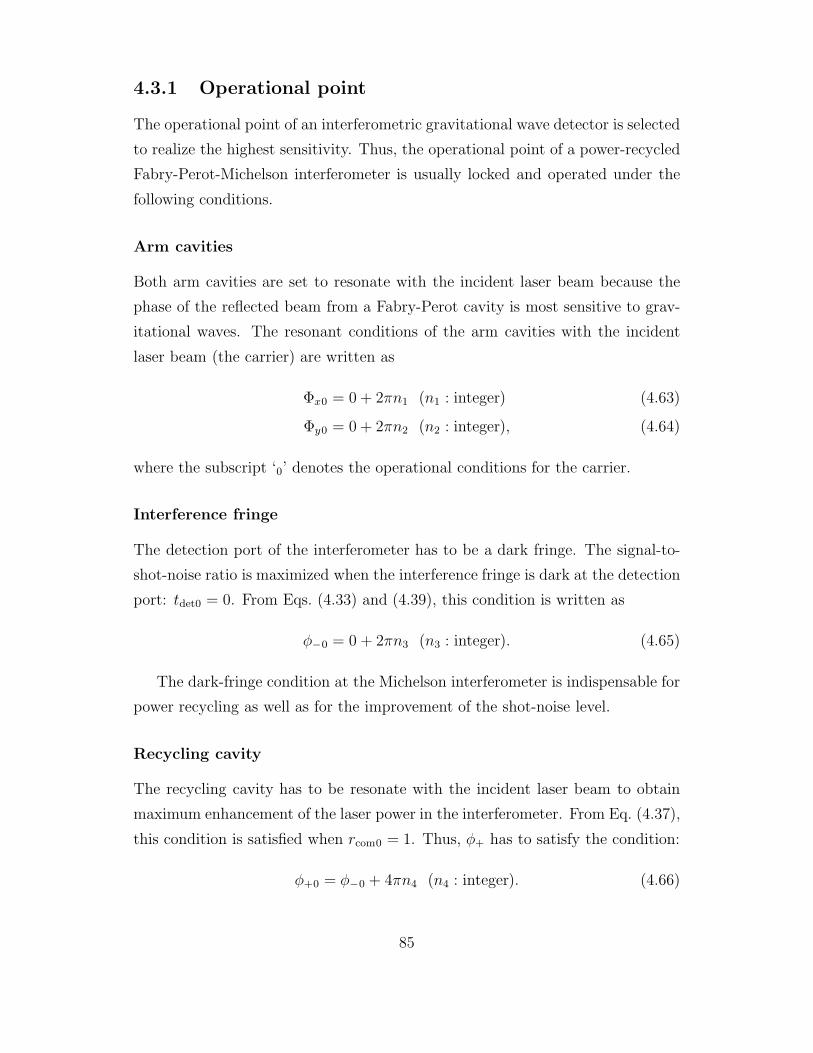
4.3.1 Operational point
The operational point of an interferometric gravitational wave detector is selected
to realize the highest sensitivity. Thus, the operational point of a power-recycled
Fabry-Perot-Michelson interferometer is usually locked and operated under the
following conditions.
Arm cavities
Both arm cavities are set to resonate with the incident laser beam because the
phase of the reflected beam from a Fabry-Perot cavity is most sensitive to grav-
itational waves. The resonant conditions of the arm cavities with the incident
laser beam (the carrier) are written as
Φx0 = 0 + 2πn1 (n1 : integer) (4.63)
Φy0 = 0 + 2πn2 (n2 : integer), (4.64)
where the subscript ‘0’ denotes the operational conditions for the carrier.
Interference fringe
The detection port of the interferometer has to be a dark fringe. The signal-to-
shot-noise ratio is maximized when the interference fringe is dark at the detection
port: tdet0 = 0. From Eqs. (4.33) and (4.39), this condition is written as
φ−0 = 0 + 2πn3 (n3 : integer). (4.65)
The dark-fringe condition at the Michelson interferometer is indispensable for
power recycling as well as for the improvement of the shot-noise level.
Recycling cavity
The recycling cavity has to be resonate with the incident laser beam to obtain
maximum enhancement of the laser power in the interferometer. From Eq. (4.37),
this condition is satisfied when rcom0 = 1. Thus, φ+ has to satisfy the condition:
φ+0 = φ−0 + 4πn4 (n4 : integer). (4.66)
85

From the Eqs. (4.63) to (4.66), the best operational point of the interferometer
is described as
Φx0 = Φy0 = φ−0 = φ+0 = 0. (4.67)
4.3.2 Conditions for the sidebands
In addition to the operational conditions for the carrier, we put a few conditions
on the modulation frequency and the length of the recycling cavity.
Phases of the sidebands
Since the carrier and sidebands have different frequencies, the round-trip phases
are different in each beam. The angular frequency of the carrier is the same as
that of the laser source (Ωl). Thus, we get the equations
Φdof0 =2LdofΩl
c(4.68)
φdof0 =2ldofΩl
c, (4.69)
where index ‘dof’ represents ‘x’, ‘y’, ‘+’, and ‘−’. Since the angular frequency of
the n-th order sideband is Ωl + nωm, we get the following equations:
Φdofn =2Ldof(Ωl + nωm)
c= Φdof0 +
2nLdofωm
c(4.70)
φdofn =2ldof(Ωl + nωm)
c= φdof0 +
2nldofωm
c. (4.71)
Here, defining the parameters α and β by
α =l−ωm
c(4.72)
β =l+ωm
c, (4.73)
we get the equation
φ−n = φ−0 + 2nα (4.74)
φ+n = φ+0 + 2nβ. (4.75)
86

Modulation frequency
The sidebands do not resonate with the arm cavity. The modulation frequency
is selected so that the first-order sidebands are near antiresonant with the arm
cavities:
Φx1 =2Lxωm
c' π + 2πn5 (n5 : integer) (4.76)
Φy1 =2Lyωm
c' π + 2πn6 (n6 : integer) (4.77)
The first-order sidebands are slightly shifted from the antiresonant condition so
that the even-order sideband should not resonate with the arm cavities. When the
finesse of the arm cavities is high enough, it is a good approximation to assume
all of the sidebands are antiresonant with the arm cavities.
Length of the recycling cavity
The first-order sidebands resonate with the recycling cavity. It is necessary to
leak the first-order sidebands to the detection port effectively, in order to increase
the sensitivity to gravitational waves. This condition is written as rcom±1 = 1,
same as the resonant condition for the carrier. Considering that the the sign of
the sidebands flips on the reflection with the arm cavities, we get the equation
β = π + 2πn7 (n7 : integer). (4.78)
From this equation, the length of the recycling cavity (l+/2) is determined de-
pending on the modulation frequency:
l+2
=c
2νm
(1
2+ n7
), (4.79)
where νm = ωm/2π is the modulation frequency. The smallest modulation fre-
quency which satisfies the resonant condition is half of the FSR of the recycling
cavity. In practice, the length of the recycling cavity is slightly shifted from the
value obtained from Eq. (4.79), because the phase change in the sidebands by the
arm cavities is not exactly π.
When the modulation frequency is slightly shifted from the antisymmetric
condition of the the arm cavity, the higher-order sidebands (|n| ≥ 2) can be
considered not to resonate with the recycling cavity, as well as the arm cavity.
87

4.3.3 Response of the interferometer at the operational
point
Here, we show the expressions for the statistic response of the interferometer
substituting the operational conditions. In the calculation, we assume some ide-
alization: the two arm cavities are identical, the beamsplitter divides the input
beam equally without any losses, and the interferometer is kept exactly at its
operational point. In addition, we neglect the effect of higher order (|n| ≥ 2)
sidebands.
Since the carrier beam is resonant with the arm cavities, the amplitude reflec-
tivity of a Fabry-Perot cavity for the carrier is written as
rcav0 = rreso = −rF +t2FrE
1 − rFrE. (4.80)
Since the sidebands are considered to be antiresonant with the arm cavities, the
reflectivity of the cavity for sidebands is written as
rcav±1 ' ranti = −rF − t2FrE
1 + rFrE. (4.81)
Differentiating the reflectivity of a Fabry-Perot cavity by the round-trip phase,
and substituting the operational conditions, we obtain
r′cav0 = r′reso =−it2FrE
(1 − rFrE)2(4.82)
r′cav±1 ' r′anti =it2FrE
(1 + rFrE)2, (4.83)
for the carrier and the sidebands, respectively.
The reflected beams by the arm cavities are recombined on the beamsplitter.
Considering the dark-fringe condition and the resonance condition of the recy-
cling cavity, we obtain the following equations for the reflectivity of the whole
interferometer for the carrier and the sidebands:
rrec0 = −rR +t2Rt2Prreso
1 − rRt2Prreso
(4.84)
rrec1 = −rR − t2Rt2Pranti cosα
1 + rRt2Pranti cos α. (4.85)
88
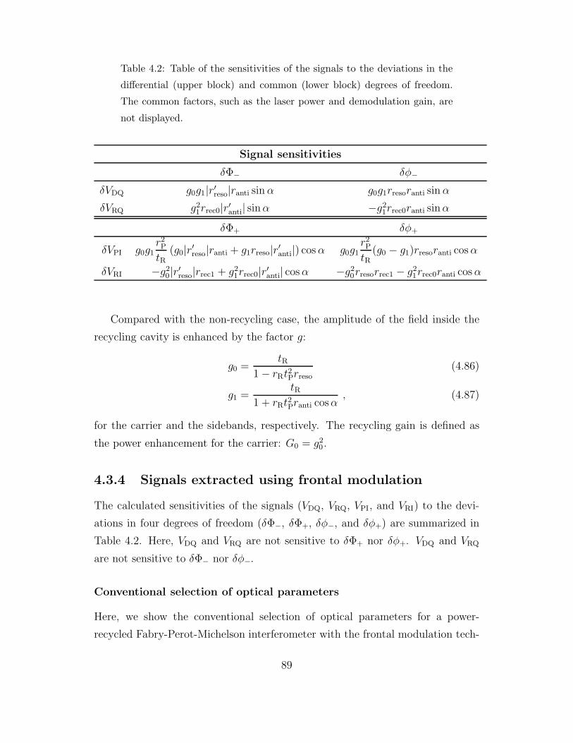
Table 4.2: Table of the sensitivities of the signals to the deviations in the
differential (upper block) and common (lower block) degrees of freedom.
The common factors, such as the laser power and demodulation gain, are
not displayed.
Signal sensitivities
δΦ− δφ−
δVDQ g0g1|r′reso|ranti sin α g0g1rresoranti sin α
δVRQ g21rrec0|r′anti| sinα −g2
1rrec0ranti sinα
δΦ+ δφ+
δVPI g0g1r2P
tR(g0|r′reso|ranti + g1rreso|r′anti|) cos α g0g1
r2P
tR(g0 − g1)rresoranti cos α
δVRI −g20|r′reso|rrec1 + g2
1rrec0|r′anti| cos α −g20rresorrec1 − g2
1rrec0ranti cos α
Compared with the non-recycling case, the amplitude of the field inside the
recycling cavity is enhanced by the factor g:
g0 =tR
1 − rRt2Prreso(4.86)
g1 =tR
1 + rRt2Pranti cosα, (4.87)
for the carrier and the sidebands, respectively. The recycling gain is defined as
the power enhancement for the carrier: G0 = g20 .
4.3.4 Signals extracted using frontal modulation
The calculated sensitivities of the signals (VDQ, VRQ, VPI, and VRI) to the devi-
ations in four degrees of freedom (δΦ−, δΦ+, δφ−, and δφ+) are summarized in
Table 4.2. Here, VDQ and VRQ are not sensitive to δΦ+ nor δφ+. VDQ and VRQ
are not sensitive to δΦ− nor δφ−.
Conventional selection of optical parameters
Here, we show the conventional selection of optical parameters for a power-
recycled Fabry-Perot-Michelson interferometer with the frontal modulation tech-
89

nique [19], and estimate of the sensitivities of the signals approximately from
Table 4.2.
The reflectivity of the end mirrors is set high so as to realize a high recycling
gain. The reflectivity of the front mirrors is selected to be slightly less than
that of the end mirror, optimizing the frequency response of the arm cavities
to the target gravitational waves. In this case, we can approximate that rreso is
slightly less than unity, ranti ' −1 and |r′reso| 1 |r′anti|. The reflectivity of the
recycling mirror is selected so as to realize a high recycling gain. From Eq. (3.68),
we can show that the recycling gain is maximized when
rR = rcom0 = t2Prreso. (4.88)
Neglecting the loss in the recycling mirror, the condition expressed by Eq. (4.88)
is also written as
rrec0 = 0. (4.89)
In practice, however, rR is set to slightly less than rcom0 for insurance against a
decrease in rreso due to contamination of the mirrors. The parameter α is selected
to be small so that the reflectivity of the compound mirror for the sidebands
(rcom1 = −t2Pranti cosα) is larger than rcom0 in order to avoid a gain constraint
on the control system [19]. Normally, the amplitude gains (g0 and g1) have
almost the same-order values. The reflectivity of the whole interferometer for the
carrier (rrec0) and for the sidebands (rrec1) also takes the same-order value. The
reflectivity of the pick-off mirror is determined considering the recycling gain and
the signal-to-noise ratio of the signal extracted from the pick-off port.
Estimation of signal sensitivity
The sensitivities of the signals are estimated from Table 4.2 with the approxi-
mated parameters.
The VDQ signal is more sensitive to a δΦ− deviation than to δl− by the phase-
change enhancement factor of the Fabry-Perot arm cavity, i.e., by the effective
bounce number of the cavity, Ncav. On the other hand, the VRQ signal is more
sensitive to a δφ− deviation than to δΦ−. Thus, the signals for differential devi-
ations of the interferometer are well-separated: the sensitivity matrix is almost
diagonal.
90

Frequency
carrier
phase change in sideband
phase change in carrier
sidebandδΦ+
δφ+
Figure 4.6: The amplitude of the laser beam output from the interferom-
eter. The carrier and sidebands experience amplitude and phase change
in the interferometer; the phase changes caused in the interferometer are
shown as phase-modulated sidebands (audio sidebands) in this Figure. The
phase change in the carrier mainly contains the enhanced δΦ+ information.
On the other hand, the phase change in the first-order sidebands mainly
contains the δφ+ information,
As for the common deviation, however, the sensitivity matrix is far from
diagonal. Since |r′reso| 1 |r′anti|, the sensitivity values are dominated by the
first terms in the δΦ+ column of Table 4.2. In the δφ+ column, the sensitivity
values are subtraction of almost the same-order terms. Thus, both VPI and VRI are
much more sensitive to the δΦ+ deviation than to δφ+. These poorly separated
signals complicate the design of the control system.
4.4 Signal-separation method
The VPI and VRI signals are more sensitive to δΦ+ than to δφ+ with the con-
ventional selection of the optical parameters. However, by selecting the optical
parameters properly, we can make the VRI signal sensitive only to the δφ+ devi-
ation. In this Section, we describe a new signal separation scheme by adjusting
the optical parameters.
91
4.4.1 Signal mixing problem
Here, we review the signal mixing problem in a power-recycled interferometer
from different viewpoint.
The signal mixing originates in the mixing of the phase change of the laser
beam. The deviations of the interferometer from the operational point cause
phase changes in the laser beam (Figure 4.6), which are detected as signals with
modulation scheme. As described in Eqs. (4.19) and (4.20), the error signals
extracted by demodulation at the modulation frequency mainly contain the in-
formation of the phase of the carrier and first-order sidebands (x0 and x±1). Thus,
the signal sensitivities are mainly contributed by two terms: the product of the
sidebands with the phase change in the carrier, and the product of the carrier
with the phase change in the sidebands.
With respect to the common motion of the interferometer (δΦ+ and δφ+), the
phase change in the carrier mainly contains the enhanced δΦ+ information and
little information about the motion in the recycling cavity. This is because the
carrier beam is resonant with the arm cavities and quite sensitive to their phase
changes. On the other hand, the phase change in the first-order sidebands mainly
contains the δφ+ information, because the sideband beams are not resonant with
the arm cavities but resonant with the recycling cavity. The phase of the side-
bands are not effected by the arm cavity motion and sensitive to the recycling
cavity motion.
Both in the carrier and the sidebands, the phase change information (con-
tained in the audio sidebands) leak to the bright fringe at interference, i.e., to
the pick-off port and reflection port. In addition, the contribution from the phase
changes in the carrier and the sidebands appear in the same demodulation phase
(in-phase). Thus, the error signals for the common motion of the interferometer
(VPI and VRI) are much more sensitive to δΦ+ than to δφ+.
4.4.2 Sideband elimination
As described above, the signals are comprised of two terms: the product of the
sidebands and the phase change in the carrier, and the product of the carrier and
the phase change in the sidebands. Thus, if the sidebands are absent and the
92

Frequency
carrier
phase change in sideband
phase change in carrier
δφ+
Figure 4.7: The amplitude of the laser beam output from the interferometer
with sideband elimination. The signal is only sensitive to the δφ+ deviation.
carrier is present in the beam incident on a photo detector, the signal contains
only information about the recycling cavity motion (Figure 4.7). This is the
essence of our signal-separation method.
It is possible to realize this condition at the reflection port, from which the
VRI signal is extracted. This condition is written by the reflectivity of the inter-
ferometer to the reflection port (rrec) as
rrec1 = 0 (4.90)
for the sidebands, and
rrec0 6= 0 (4.91)
for the carrier.
4.4.3 Adjustment of the optical parameters
From Eq. (4.38), Eq. (4.90) is also written as
rR = −t2Pranti cos α = rcom1. (4.92)
This equation shows that the reflectivity of the compound mirror for sidebands
is equal to that of the recycling mirror. In other words, the gain of the sidebands
is maximized.
93
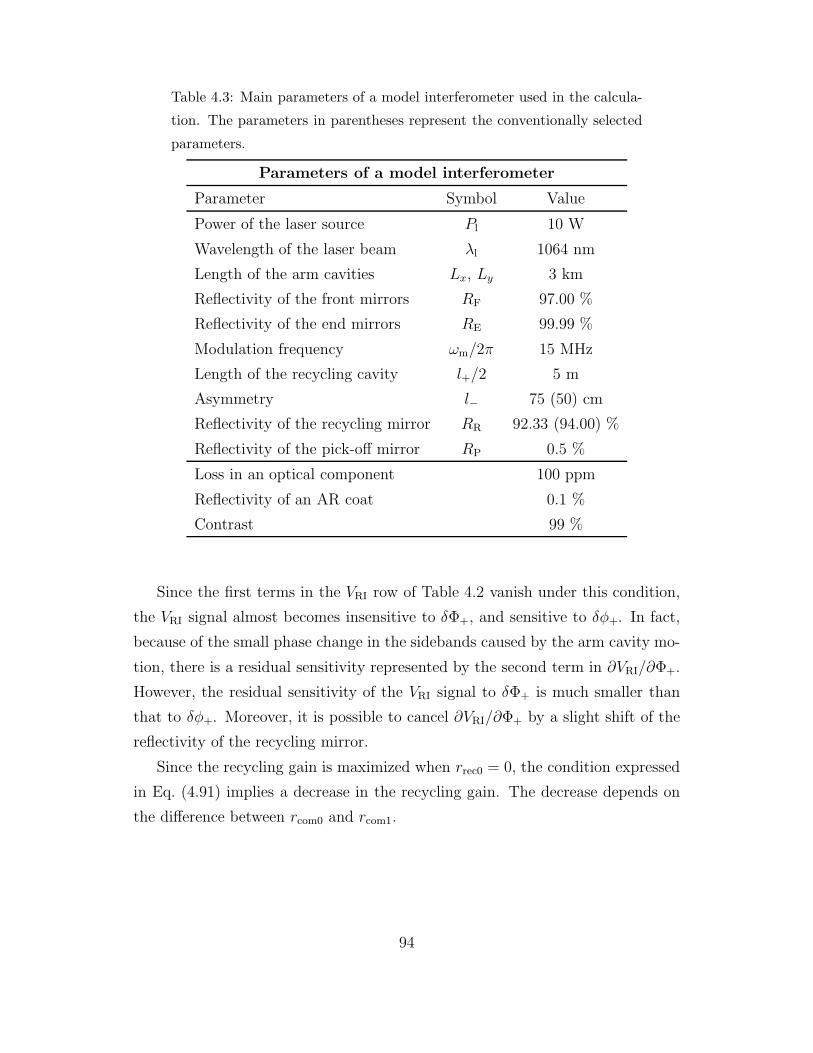
Table 4.3: Main parameters of a model interferometer used in the calcula-
tion. The parameters in parentheses represent the conventionally selected
parameters.
Parameters of a model interferometer
Parameter Symbol Value
Power of the laser source Pl 10 W
Wavelength of the laser beam λl 1064 nm
Length of the arm cavities Lx, Ly 3 km
Reflectivity of the front mirrors RF 97.00 %
Reflectivity of the end mirrors RE 99.99 %
Modulation frequency ωm/2π 15 MHz
Length of the recycling cavity l+/2 5 m
Asymmetry l− 75 (50) cm
Reflectivity of the recycling mirror RR 92.33 (94.00) %
Reflectivity of the pick-off mirror RP 0.5 %
Loss in an optical component 100 ppm
Reflectivity of an AR coat 0.1 %
Contrast 99 %
Since the first terms in the VRI row of Table 4.2 vanish under this condition,
the VRI signal almost becomes insensitive to δΦ+, and sensitive to δφ+. In fact,
because of the small phase change in the sidebands caused by the arm cavity mo-
tion, there is a residual sensitivity represented by the second term in ∂VRI/∂Φ+.
However, the residual sensitivity of the VRI signal to δΦ+ is much smaller than
that to δφ+. Moreover, it is possible to cancel ∂VRI/∂Φ+ by a slight shift of the
reflectivity of the recycling mirror.
Since the recycling gain is maximized when rrec0 = 0, the condition expressed
in Eq. (4.91) implies a decrease in the recycling gain. The decrease depends on
the difference between rcom0 and rcom1.
94

Table 4.4: Sensitivities of the signals in the deviation in the four degrees of
freedom (extracted by the conventional frontal modulation technique).
Signal sensitivities (without signal separation)
δΦ− δφ− δΦ+ δφ+
VDQ 1 7.6 × 10⁻³ 0 0
VRQ 7.6 × 10⁻³ 1 0 0
VPI 0 0 1 1.1 × 10⁻⁴
VRI 0 0 1 8.0× 10⁻⁴
4.4.4 Calculation of the signals in a model interferometer
In order to evaluate our signal-separation method, we prepared a model interfero-
metric gravitational wave detector and calculated the sensitivities of the extracted
signals. The parameters of the model interferometer are shown in Table 4.3. The
parameters in the parentheses represent the conventionally selected parameters.
In this numerical calculation, the effect of losses in the optical parameters and
contrast defect were considered.
Without signal separation
At first, we calculated the sensitivities of the signals extracted by the conven-
tional frontal modulation technique. The reflectivity of the recycling mirror
(RR = 0.9400) is slightly less than that of the compound mirror for the car-
rier (Rcom0 = 0.9513). The asymmetry (l− = 50 cm) is selected so as to avoid any
gain constraint. Table 4.4 gives the sensitivity matrix of the model interferome-
ter. The values in the matrix are normalized so that the largest sensitivity value
in each row is equal to unity. Though the signals corresponding to the deviations
in the four degrees of freedom are extracted, both the VPI and VRI signals are
more sensitive to δΦ+ than to δφ+. The calculated recycling gain is 20.2.
With signal separation
Next, we calculated the sensitivities of the signals by our method. In this cal-
culation, the asymmetry was 75 cm, and thus, the reflectivity of the recycling
95

Table 4.5: Sensitivities of the signals to the deviations in the four degrees
of freedom (extracted by modified frontal modulation technique).
Signal sensitivities (with signal separation)
δΦ− δφ− δΦ+ δφ+
VDQ 1 7.6 × 10⁻³ 0 0
VRQ 7.6 × 10⁻³ 1 0 0
VPI 0 0 1 1.3 × 10⁻³
VRI 0 0 7.8 × 10⁻³ 1
mirror became 92.33% from Eq. (4.92). Table 4.5 is the sensitivity matrix of
the extracted signals with these parameters. The diagonal values are the main
signals necessary for controlling the interferometer, while the off-diagonal values
represent the mixing of unnecessary signals. The VDQ, VRQ, VPI, and VRI signals
are most sensitive to the deviations δΦ−, δφ−, δΦ+, and δφ+, respectively. The
off-diagonal terms in the sensitivity matrix are less than 1 % of the diagonal
terms. The calculated recycling gain is 19.4; this is 96% of the value when the
reflectivity of the recycling mirror is set to maximize it. The shot-noise level of
VDQ signal for δL− is 5.3×10⁻²⁰ m/√
Hz, which corresponds to a strain sensitivity
of 1.8 × 10⁻²³ /√
Hz for the gravitational wave signal.
4.4.5 Requirements for signal separation
Reflectivity matching
Our power recycling scheme differs from the conventional one in only one point;
the condition rrec1 = 0, Eq. (4.90), is required in place of rrec0 = 0, Eq. (4.89).
The sensitivity matrix is diagonalized remarkably well if Eq. (4.90) is satisfied.
However, it is difficult to realize this condition exactly because a high accuracy
is required for the reflectivity of the recycling mirror. Figure 4.8 shows the re-
quired accuracy as a function of the reflectivity of the recycling mirror when the
sensitivity of the VRI signal to δΦ+ is required to be less than 10% of that to δφ+
in the model interferometer. The reflectivity of the recycling mirror is changed
together with the asymmetry under the condition represented by Eq. (4.92). The
96
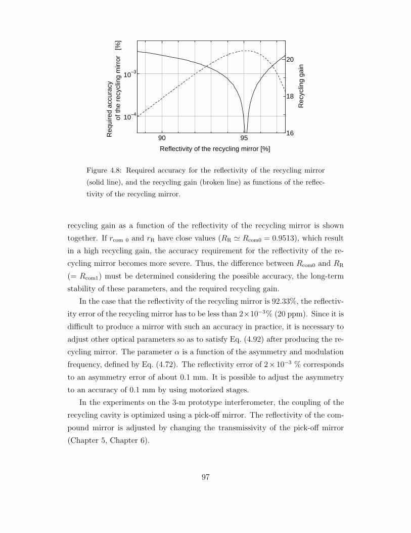
90 95
10–4
10–3
16
18
20
Reflectivity of the recycling mirror [%]
Req
uire
d ac
cura
cy
Rec
yclin
g ga
in
of th
e re
cycl
ing
mirr
or
[%]
Figure 4.8: Required accuracy for the reflectivity of the recycling mirror
(solid line), and the recycling gain (broken line) as functions of the reflec-
tivity of the recycling mirror.
recycling gain as a function of the reflectivity of the recycling mirror is shown
together. If rcom 0 and rR have close values (RR ' Rcom0 = 0.9513), which result
in a high recycling gain, the accuracy requirement for the reflectivity of the re-
cycling mirror becomes more severe. Thus, the difference between Rcom0 and RR
(= Rcom1) must be determined considering the possible accuracy, the long-term
stability of these parameters, and the required recycling gain.
In the case that the reflectivity of the recycling mirror is 92.33%, the reflectiv-
ity error of the recycling mirror has to be less than 2×10⁻³% (20 ppm). Since it is
difficult to produce a mirror with such an accuracy in practice, it is necessary to
adjust other optical parameters so as to satisfy Eq. (4.92) after producing the re-
cycling mirror. The parameter α is a function of the asymmetry and modulation
frequency, defined by Eq. (4.72). The reflectivity error of 2×10⁻³ % corresponds
to an asymmetry error of about 0.1 mm. It is possible to adjust the asymmetry
to an accuracy of 0.1 mm by using motorized stages.
In the experiments on the 3-m prototype interferometer, the coupling of the
recycling cavity is optimized using a pick-off mirror. The reflectivity of the com-
pound mirror is adjusted by changing the transmissivity of the pick-off mirror
(Chapter 5, Chapter 6).
97

Fluctuation of the reflectivity
In addition to the initial deviation from the optimal coupling described above,
the fluctuation of the interferometer can cause the signal mixing. The reflectivity
of the compound mirror fluctuates because the fluctuation of the interferometer
is suppressed only with finite control gains.
The fluctuation of the arm cavity length (δL−, δL+) cause a very small effect
on the reflectivity change of the compound mirror for the sidebands because
sidebands are almost antiresonant with the arm cavity. However, the fluctuation
of interference fringe (δl−) changes the reflectivity of the compound mirror. To
keep the reflectivity fluctuation less than 2× 10⁻³%, the residual RMS deviation
from the operational point should be less than 5 × 10⁻¹⁰ m. This value is about
the same order as that required from rejection of intensity noise level in the
interferometer.
The fluctuation of mirror orientation also changes the reflectivity of the com-
pound mirror because of imperfect interference on the beamsplitter. To keep
the reflectivity fluctuation less than 2× 10⁻³%, the RMS deviation of the mirror
orientation should be less than 8 × 10⁻⁸ rad in the model interferometer [71].
Effects of the higher-order sidebands
In the calculation of signal sensitivity (Section 4.3), we neglected the effect of the
higher-order sidebands. However, the higher-order sidebands can extinguish the
δl+ signal under the signal-separation condition.
In the reflection port, the effect of second-order sidebands are relatively en-
hanced. The reflectivity of the interferometer to the reflection port is small for the
carrier and the first-order sidebands because the carrier and the first-order side-
bands are resonant with the recycling cavity. On the other hand, since the second-
order sidebands are antiresonant with the recycling cavity, almost all power of the
second-order sidebands is reflected back to the reflection port. The second-order
sidebands produce the δl+ signals coupling with the phase change in the first-
order sidebands, which can cancel out the δl+ signal in the error signal without
proper selection of the optical parameters.
98

Adjustment of recycling cavity length
The length of the recycling cavity is determined so that the first-order sidebands
as well as the carrier are resonant with the recycling cavity. Here, if the recycling
cavity length is not set properly, the sidebands cannot be rejected from the reflec-
tion port. The misadjustment of the recycling cavity length and the modulation
frequency cause a mixing of δL+ signal to the reflection port signals (δl−, δl+),
and excess intensity noise coupling with the frequency noise.
Putting the same requirement for the residual sidebands at the reflection port
as the above requirements, the recycling cavity length error has to be less than
2 × 10⁻⁵ m. This length error corresponds to the modulation frequency error of
50 Hz.
99
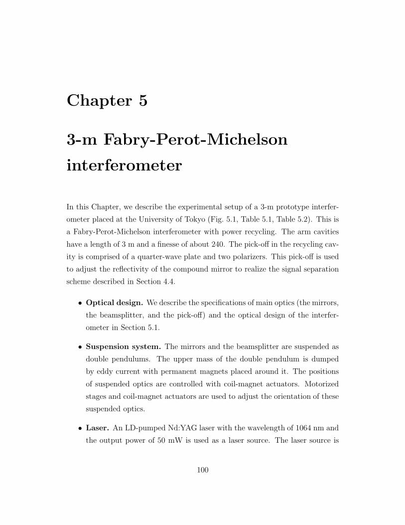
Chapter 5
3-m Fabry-Perot-Michelson
interferometer
In this Chapter, we describe the experimental setup of a 3-m prototype interfer-
ometer placed at the University of Tokyo (Fig. 5.1, Table 5.1, Table 5.2). This is
a Fabry-Perot-Michelson interferometer with power recycling. The arm cavities
have a length of 3 m and a finesse of about 240. The pick-off in the recycling cav-
ity is comprised of a quarter-wave plate and two polarizers. This pick-off is used
to adjust the reflectivity of the compound mirror to realize the signal separation
scheme described in Section 4.4.
• Optical design. We describe the specifications of main optics (the mirrors,
the beamsplitter, and the pick-off) and the optical design of the interfer-
ometer in Section 5.1.
• Suspension system. The mirrors and the beamsplitter are suspended as
double pendulums. The upper mass of the double pendulum is dumped
by eddy current with permanent magnets placed around it. The positions
of suspended optics are controlled with coil-magnet actuators. Motorized
stages and coil-magnet actuators are used to adjust the orientation of these
suspended optics.
• Laser. An LD-pumped Nd:YAG laser with the wavelength of 1064 nm and
the output power of 50 mW is used as a laser source. The laser source is
100

Recycling mirror
Beamsplitter
End mirror
Laser source
End mirrorFront mirror
Input laser table
Recycling tankCenter tank End tank
End tank
EOM
AOM
CL
L
W
PD3
PD9
SC
FI
L
L
λ/2
λ/4
PD1PD5
PD4
PD2
PD6
PLPD7
PD8
Figure
5.1:E
xperimentalsetup
of3m
Fabry-Perot-M
ichelsoninterferom
eter.
101

Table 5.1: Main features of the 3-m prototype interferometer.
Features of the 3-m prototype interferometer
Interferometer type Fabry-Perot-Michelson interferometer
with power recycling
Laser source LD-pumped Nd:YAG laser (1064 nm)
Suspension system Double pendulum
damped by eddy current
Signal extraction Frontal modulation
with the signal separation scheme
Vacuum system Four tanks connected with vacuum tubes
evacuated with a scroll pump
placed on an input table. The laser beam is introduced to the interferom-
eter after passing through lenses for mode matching, an EOM for phase
modulation, an AOM for intensity modulation, and Faraday isolators.
• Signal-extraction and control system. The interferometer is kept at
the operational point by controlling the lengths between the mirrors. The
control signals are extracted with the signal-separation scheme described in
Chapter 4; the modulation, demodulation and control system is shown in
Section 5.4. The photo detectors for the control of the interferometer are
placed in the center tank and the input table.
• Devices for monitor and measurement. Several devices are placed to
diagnose the status of the interferometer: AF photo detectors for monitoring
the laser power, and an optical spectrum analyzer for the measurement of
the reflected sidebands.
• Vacuum system. The interferometer is housed in a vacuum system com-
prised of a recycling tank, center tank, two end tanks, and vacuum tubes.
The vacuum system is evacuated with a scroll pump.
102

Table 5.2: Main parameters of the 3-m prototype interferometer.
Parameters of the 3-m prototype interferometer
Parameter Symbol Value
Power of the laser source Pl 35 mW
Wavelength of the laser beam λl 1064 nm
Modulation frequency ωm/2π 40.265 MHz
Modulation index mm 0.58 rad
Length of the arm cavities Lx, Ly 2.95 m
Length of the recycling cavity l+/2 1.82 m
Asymmetry l− 15 cm
Reflectivity of the front mirrors RF 97.4 %, 97.1 %
Reflectivity of the end mirrors RE 99.6 %, 99.9 %
Reflectivity of the recycling mirror RR 63.6 %
Reflectivity of the pick-off mirror RP adjustable
Finesse of the arm cavities F 230
Power recycling gain G0 2.5 (TP = 0.872)
Power gain for the sidebands G1 3.3 (TP = 0.872)
103

Table 5.3: Specifications of the mirrors of the 3-m interferometer.
Mirrors
Front mirror End mirror Recycling mirror
Diameter 30 mm 30 mm 30 mm
Thickness 5 mm 5 mm 5 mm
Curvature ∞ (flat) 4.5 m 4.28 m
Reflectivity 97.5% 99.9% 60%
Measured (x arm) 97.4% 99.6%
reflectivity (y arm) 97.1% 99.9%63.6%
5.1 Optical design
In this Section, we show the optical design of the 3-m prototype interferometer.
This interferometer is a Michelson interferometer with Fabry-Perot arm cavities.
In addition, power recycling is applied to this interferometer.
5.1.1 Mirrors
The interferometer is comprised of five main mirrors: two front mirrors, two
end mirrors, and a recycling mirror. Table 5.3 shows the specifications of these
mirrors. Though the reflectivities of mirrors are selected in a similar way as a
real large gravitational wave detector, they are selected to be suitable values for
our experimental purposes. The reflectivity of the front mirrors is selected to
realize sufficiently high finesse about a few hundred1. The reflectivity of the end
mirrors is selected high so as to obtain a high reflectivity of the cavities, which is
necessary to realize a high recycling gain2. With the reflectivities of 97.5 % (front
mirror) and 99.9 % (end mirror), the arm cavity have a finesse of about 240 and
1The finesse is usually selected so that the cut-off frequency of the cavity would be near the
observation band of gravitational waves in a real gravitational wave detector. A finesse of one
hundred results in a cut-off frequency about a few hundred hertz in a km-class interferometer.
In the 3-m interferometer the cut-off frequency is about one hundred kHz.2It is possible to make a mirror with higher reflectivity. However, it is not easy to keep such
a high reflectivity with our experimental environment. For the purpose of our experiment, the
reflectivity of 99.9% for the end mirrors is sufficient.
104
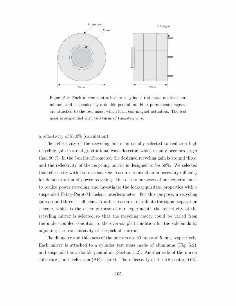
Al test mass
700 mm
Mirror
Nd magnet
500 mm
Figure 5.2: Each mirror is attached to a cylinder test mass made of alu-
minum, and suspended by a double pendulum. Four permanent magnets
are attached to the test mass, which form coil-magnet actuators. The test
mass is suspended with two turns of tungsten wire.
a reflectivity of 83.0% (calculation).
The reflectivity of the recycling mirror is usually selected to realize a high
recycling gain in a real gravitational wave detector, which usually becomes larger
than 90 %. In the 3-m interferometer, the designed recycling gain is around three,
and the reflectivity of the recycling mirror is designed to be 60%. We selected
this reflectivity with two reasons. One reason is to avoid an unnecessary difficulty
for demonstration of power recycling. One of the purposes of our experiment is
to realize power recycling and investigate the lock-acquisition properties with a
suspended Fabry-Perot-Michelson interferometer. For this purpose, a recycling
gain around three is sufficient. Another reason is to evaluate the signal-separation
scheme, which is the other purpose of our experiment: the reflectivity of the
recycling mirror is selected so that the recycling cavity could be varied from
the under-coupled condition to the over-coupled condition for the sidebands by
adjusting the transmissivity of the pick-off mirror.
The diameter and thickness of the mirrors are 30 mm and 5 mm, respectively.
Each mirror is attached to a cylinder test mass made of aluminum (Fig. 5.2),
and suspended as a double pendulum (Section 5.2). Another side of the mirror
substrate is anti-reflection (AR) coated. The reflectivity of the AR coat is 0.6%.
105
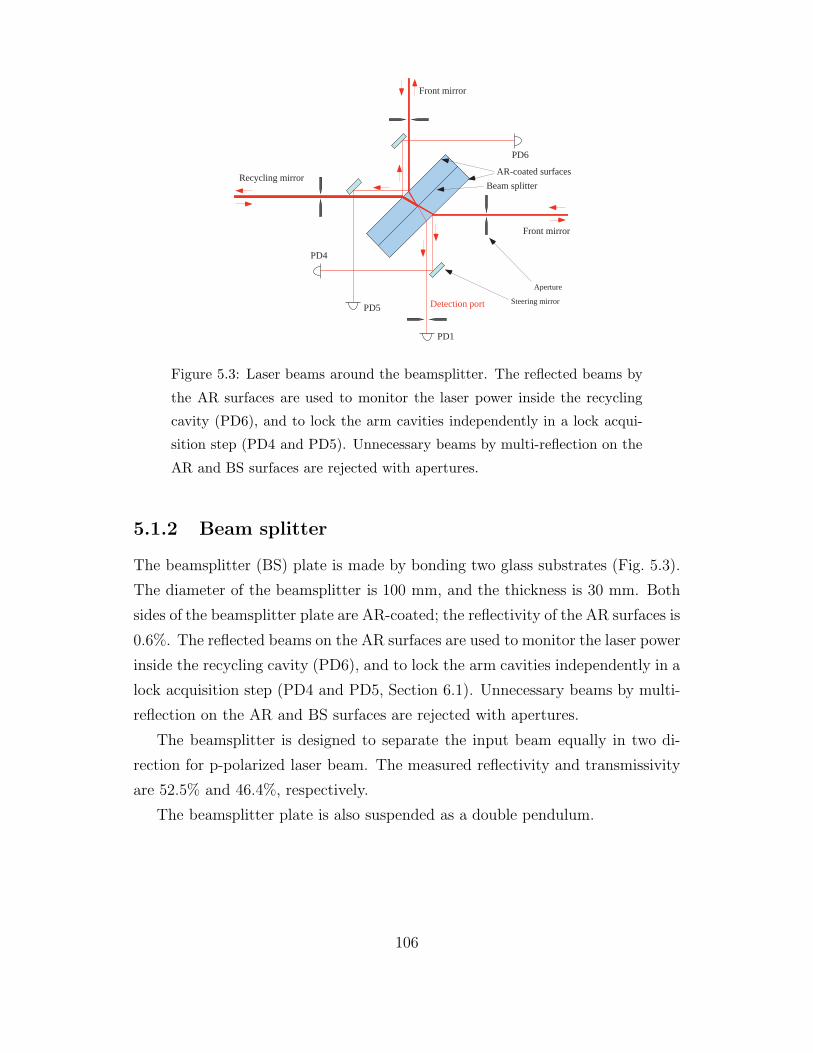
Recycling mirror
Front mirror
Front mirror
PD1
Detection port
PD4
PD5
PD6
Beam splitter
Steering mirror
Aperture
AR-coated surfaces
Figure 5.3: Laser beams around the beamsplitter. The reflected beams by
the AR surfaces are used to monitor the laser power inside the recycling
cavity (PD6), and to lock the arm cavities independently in a lock acqui-
sition step (PD4 and PD5). Unnecessary beams by multi-reflection on the
AR and BS surfaces are rejected with apertures.
5.1.2 Beam splitter
The beamsplitter (BS) plate is made by bonding two glass substrates (Fig. 5.3).
The diameter of the beamsplitter is 100 mm, and the thickness is 30 mm. Both
sides of the beamsplitter plate are AR-coated; the reflectivity of the AR surfaces is
0.6%. The reflected beams on the AR surfaces are used to monitor the laser power
inside the recycling cavity (PD6), and to lock the arm cavities independently in a
lock acquisition step (PD4 and PD5, Section 6.1). Unnecessary beams by multi-
reflection on the AR and BS surfaces are rejected with apertures.
The beamsplitter is designed to separate the input beam equally in two di-
rection for p-polarized laser beam. The measured reflectivity and transmissivity
are 52.5% and 46.4%, respectively.
The beamsplitter plate is also suspended as a double pendulum.
106

0 90 180
60
80
100
Angle of the λ/4 plate [deg]
Tra
nsm
issi
vity
[%]
Figure 5.4: The transmissivity of the pick-off mirror composed with a λ/4
plate and two polarizers. The dots and the solid curve represent the mea-
sured and fitted transmissivity. The transmissivity is varied by rotating
the λ/4 plate. The maxim and minimum transmissivities of this pick-off
are 98.9% and 48.3%, respectively.
5.1.3 Pick-off mirror
In order to realize the signal-separation scheme (Chapter 4), the reflectivity of
the recycling mirror RR has to be set equal to that of the compound mirror for
the sidebands Rcom1. However, it is not easy to produce a mirror setting the
reflectivity in a high accuracy. In addition, the reflectivity of the compound
mirror depends on the condition of the interferometer: the mirror contamination
and the alignment of the interferometer3.
The signal-separation condition is written by the equation RR = Rcom1 'T 2
P cos2 α as described in Eq. 4.92. Thus, instead of adjusting the reflectivity
of the recycling mirror, the signal separation is also realized by adjusting the
reflectivity of the compound mirror for the sidebands. In the 3-m interferometer,
the pick-off in the recycling cavity is formed with a λ/4 plate and two polarizers;
the transmissivity of the pick-off mirror is variable by rotating the λ/4 plate,
which is mounted in a motorized rotary stage. Figure 5.4 shows the measured
transmissivity of the pick-off mirror. The maxim and minimum transmissivities of
3However, the effect of the mirror contamination is not as serious for Rcom1 as that for Rcom0
because the sidebands do not enter the arm cavity.
107
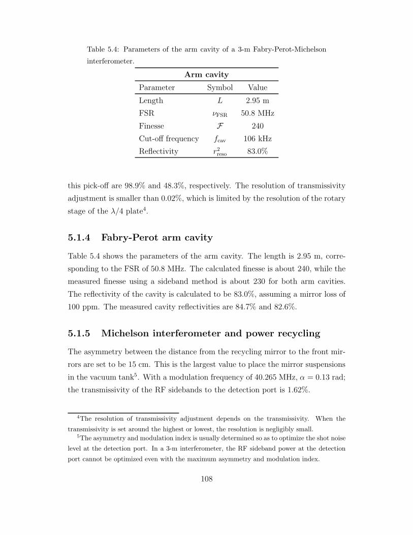
Table 5.4: Parameters of the arm cavity of a 3-m Fabry-Perot-Michelson
interferometer.
Arm cavity
Parameter Symbol Value
Length L 2.95 m
FSR νFSR 50.8 MHz
Finesse F 240
Cut-off frequency fcav 106 kHz
Reflectivity r2reso 83.0%
this pick-off are 98.9% and 48.3%, respectively. The resolution of transmissivity
adjustment is smaller than 0.02%, which is limited by the resolution of the rotary
stage of the λ/4 plate4.
5.1.4 Fabry-Perot arm cavity
Table 5.4 shows the parameters of the arm cavity. The length is 2.95 m, corre-
sponding to the FSR of 50.8 MHz. The calculated finesse is about 240, while the
measured finesse using a sideband method is about 230 for both arm cavities.
The reflectivity of the cavity is calculated to be 83.0%, assuming a mirror loss of
100 ppm. The measured cavity reflectivities are 84.7% and 82.6%.
5.1.5 Michelson interferometer and power recycling
The asymmetry between the distance from the recycling mirror to the front mir-
rors are set to be 15 cm. This is the largest value to place the mirror suspensions
in the vacuum tank5. With a modulation frequency of 40.265 MHz, α = 0.13 rad;
the transmissivity of the RF sidebands to the detection port is 1.62%.
4The resolution of transmissivity adjustment depends on the transmissivity. When the
transmissivity is set around the highest or lowest, the resolution is negligibly small.5The asymmetry and modulation index is usually determined so as to optimize the shot noise
level at the detection port. In a 3-m interferometer, the RF sideband power at the detection
port cannot be optimized even with the maximum asymmetry and modulation index.
108
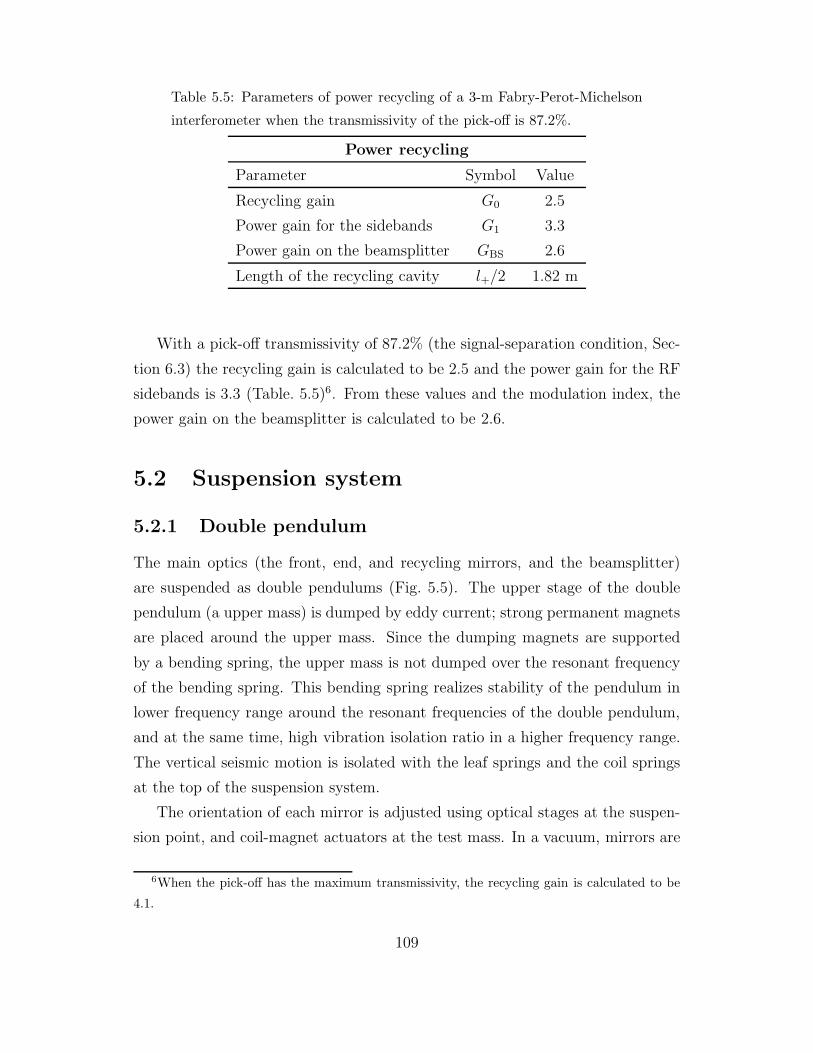
Table 5.5: Parameters of power recycling of a 3-m Fabry-Perot-Michelson
interferometer when the transmissivity of the pick-off is 87.2%.
Power recycling
Parameter Symbol Value
Recycling gain G0 2.5
Power gain for the sidebands G1 3.3
Power gain on the beamsplitter GBS 2.6
Length of the recycling cavity l+/2 1.82 m
With a pick-off transmissivity of 87.2% (the signal-separation condition, Sec-
tion 6.3) the recycling gain is calculated to be 2.5 and the power gain for the RF
sidebands is 3.3 (Table. 5.5)6. From these values and the modulation index, the
power gain on the beamsplitter is calculated to be 2.6.
5.2 Suspension system
5.2.1 Double pendulum
The main optics (the front, end, and recycling mirrors, and the beamsplitter)
are suspended as double pendulums (Fig. 5.5). The upper stage of the double
pendulum (a upper mass) is dumped by eddy current; strong permanent magnets
are placed around the upper mass. Since the dumping magnets are supported
by a bending spring, the upper mass is not dumped over the resonant frequency
of the bending spring. This bending spring realizes stability of the pendulum in
lower frequency range around the resonant frequencies of the double pendulum,
and at the same time, high vibration isolation ratio in a higher frequency range.
The vertical seismic motion is isolated with the leaf springs and the coil springs
at the top of the suspension system.
The orientation of each mirror is adjusted using optical stages at the suspen-
sion point, and coil-magnet actuators at the test mass. In a vacuum, mirrors are
6When the pick-off has the maximum transmissivity, the recycling gain is calculated to be
4.1.
109
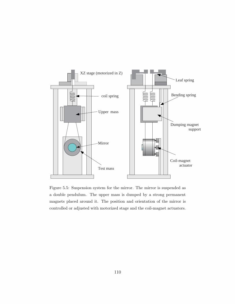
coil spring
XZ stage (motorized in Z)
Bending spring
Upper mass
Mirror
Test mass
Coil-magnet actuator
Dumping magnet support
Leaf spring
Figure 5.5: Suspension system for the mirror. The mirror is suspended as
a double pendulum. The upper mass is dumped by a strong permanent
magnets placed around it. The position and orientation of the mirror is
controlled or adjusted with motorized stage and the coil-magnet actuators.
110

10–1 100 101 10210–5
10–4
10–3
10–2
10–1
100
101
Frequency [Hz]
Vib
ratio
n is
olat
ion
ratio
Figure 5.6: Vibration isolation ratio of the suspension system. The isolation
ratio is degraded by resonances of the suspension system.
aligned with motorized micro stages (in a pitch direction) and the coil-magnet
actuators (in a yaw direction). No active control of the alignment is applied to
the 3-m interferometer.
5.2.2 Isolation ratio
The vibration isolation ratio, the ratio of the motion of the suspension point to
that of the mirror mass, is measured by shaking the suspension system. The
measured vibration isolation ratio is shown in Fig. 5.6 [72]. The mirror motion
at the resonance of the pendulum around 1 Hz is damped with the permanent
magnets. The vibration isolation ratio is about 3 × 10⁻² at 10 Hz, and 3 × 10⁻⁴
at 100 Hz. The ratio is degraded from the ideal case because of the resonances
of the suspension system.
5.2.3 Coil-magnet actuator
In order to to keep the interferometer at the operational point, it is necessary to
control the position of the suspended optical components. The mirror position is
controlled with permanent magnets attached on the back of a mirror test mass
and coils placed nearby the magnets. The strong Nd permanent magnets attached
to the test mass have a length of 10 mm and a diameter of 2 mm.
111

Table 5.6: Actuator efficiencies at 3 kHz; the mirror displacement caused
by voltage input to the coil driver. The efficiency of the PZT on the laser
source is shown together.
Actuators
Actuator Efficiency
Front mirror (x) 5.2 × 10⁻¹² m/V
Front mirror (y) 3.4 × 10⁻¹² m/V
Beam splitter 2.0 × 10⁻¹² m/V
Recycling mirror 3.8 × 10⁻¹² m/V
PZT 2.59 MHz/V
Two coil-magnet actuators (upper and lower actuators) are used to control
the longitudinal position (in the direction along the laser beam) of the test mass.
The other two actuators are used to adjust the angle of the test mass (in the yaw
direction).
Calibration of the mirror actuators
The efficiency of a coil-magnet actuator is described by the transfer function from
the input voltage into the coil diver to the displacement of the test mass. The
actuator efficiencies of the front mirrors and the beamsplitter are calibrated with
the simple front-mirror Michelson interferometer controlled with a differential
method.
The efficiency of the actuator of the recycling mirror is measured with a cavity
comprised of the recycling mirror and one of the front mirror, comparing the
output signal when each of the front mirror and the recycling mirror is shaken.
The measured efficiency of the actuators measured at 3 kHz are summarized in
Table 5.6. The efficiency of the PZT on the laser head is also described together.
These efficiencies of the actuators are used to calibrate the error signals and to
estimate the signal-mixing ratio under operation of the interferometer.
112
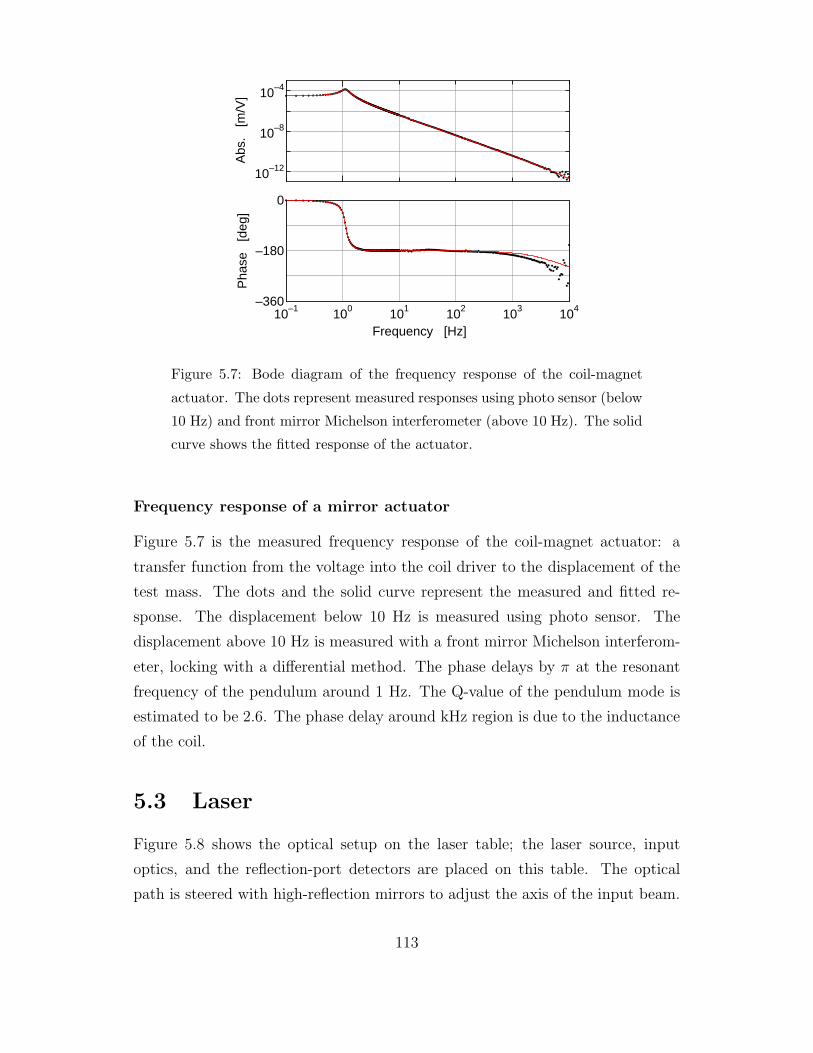
10–12
10–8
10–4
10–1 100 101 102 103 104–360
–180
0
Abs
. [m
/V]
Pha
se
[deg
]
Frequency [Hz]
Figure 5.7: Bode diagram of the frequency response of the coil-magnet
actuator. The dots represent measured responses using photo sensor (below
10 Hz) and front mirror Michelson interferometer (above 10 Hz). The solid
curve shows the fitted response of the actuator.
Frequency response of a mirror actuator
Figure 5.7 is the measured frequency response of the coil-magnet actuator: a
transfer function from the voltage into the coil driver to the displacement of the
test mass. The dots and the solid curve represent the measured and fitted re-
sponse. The displacement below 10 Hz is measured using photo sensor. The
displacement above 10 Hz is measured with a front mirror Michelson interferom-
eter, locking with a differential method. The phase delays by π at the resonant
frequency of the pendulum around 1 Hz. The Q-value of the pendulum mode is
estimated to be 2.6. The phase delay around kHz region is due to the inductance
of the coil.
5.3 Laser
Figure 5.8 shows the optical setup on the laser table; the laser source, input
optics, and the reflection-port detectors are placed on this table. The optical
path is steered with high-reflection mirrors to adjust the axis of the input beam.
113
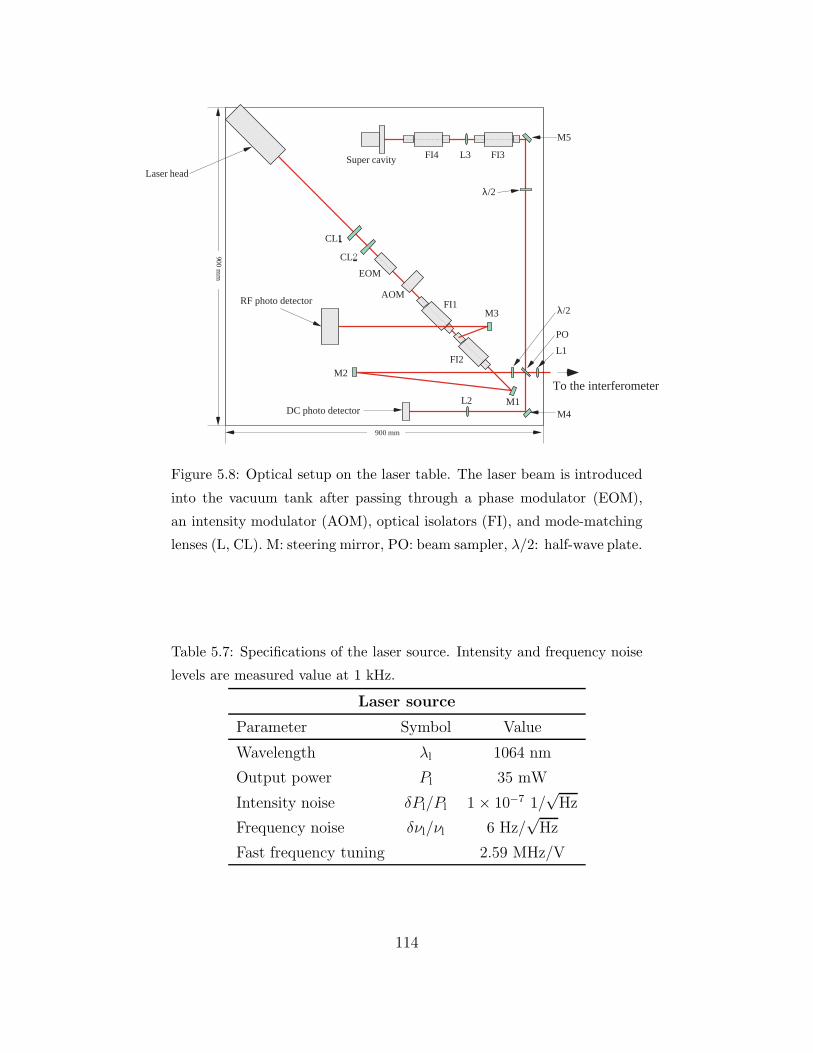
Laser head
RF photo detector
DC photo detector
M2
M3
M5
M4
L3
L2
L1
CL
CL
EOM
AOMFI1
FI2
M1
To the interferometer
900 mm
FI3FI4Super cavity
PO
λ/2
λ/2
Figure 5.8: Optical setup on the laser table. The laser beam is introduced
into the vacuum tank after passing through a phase modulator (EOM),
an intensity modulator (AOM), optical isolators (FI), and mode-matching
lenses (L, CL). M: steering mirror, PO: beam sampler, λ/2: half-wave plate.
Table 5.7: Specifications of the laser source. Intensity and frequency noise
levels are measured value at 1 kHz.
Laser source
Parameter Symbol Value
Wavelength λl 1064 nm
Output power Pl 35 mW
Intensity noise δPl/Pl 1 × 10⁻⁷ 1/√
Hz
Frequency noise δνl/νl 6 Hz/√
Hz
Fast frequency tuning 2.59 MHz/V
114

105
106
107
101 102 103 104 105–180
0
180
Abs
. [H
z/v]
Pha
se
[deg
]
Frequency [Hz]
Figure 5.9: Bode diagram of frequency response of the PZT actuator of the
laser source measured by one of the arm cavities. The response of the PZT
is almost flat up to 100 kHz. The phase dilation is due to the cut-off of the
cavity. The frequency tuning efficiency of the PZT is estimated to be 2.59
MHz/V from this measurement.
5.3.1 Laser source
As a laser source, we use a laser-diode pumped Nd:YAG laser7 (LIGHTWAVE
electronics, model 124-1064-050-F) comprised of a monolithic non-planar ring os-
cillator (NPRO). The specifications of the laser source is summarized in Table 5.7.
The wavelength is 1064 nm and the output power is about 50 mW. However, the
laser power introduced into the interferometer is reduced to 35 mW because of
the insertion losses of a phase modulator and isolators and so on.
The output frequency can be tuned with a piezoelectric element (PZT) bonded
onto the laser crystal, and with a thermoelectric cooler under the crystal. Fig-
ure 5.9 shows a measured frequency response of PZT using one of the arm cavities.
The response of the PZT actuator is almost flat up to 100 kHz, and the frequency
tuning efficiency is 2.59 MHz/V. Using a relation of the response of a Fabry-Perot
cavity to the frequency and displacement changes: |δL| = |δνl/νl|L, the corre-
7Since Nd:YAG laser has good frequency and intensity noise properties, it will also be used
in interferometric gravitational wave detectors under construction [11, 12, 13, 14].
115
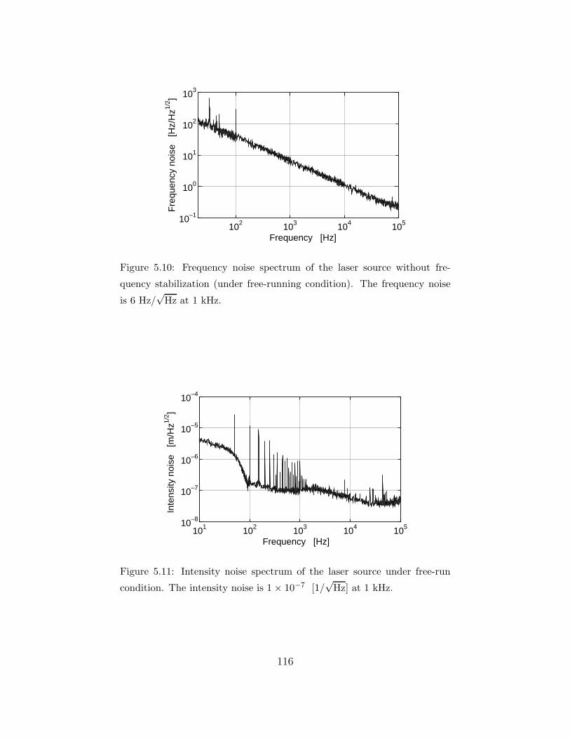
102 103 104 10510–1
100
101
102
103
Frequency [Hz]
Fre
quen
cy n
oise
[H
z/H
z1/2 ]
Figure 5.10: Frequency noise spectrum of the laser source without fre-
quency stabilization (under free-running condition). The frequency noise
is 6 Hz/√
Hz at 1 kHz.
101 102 103 104 10510–8
10–7
10–6
10–5
10–4
Frequency [Hz]
Inte
nsity
noi
se
[m/H
z1/2 ]
Figure 5.11: Intensity noise spectrum of the laser source under free-run
condition. The intensity noise is 1 × 10⁻⁷ [1/√
Hz] at 1 kHz.
116

0 1 2 3 4 5 6 7Distance from the laser head [m]
Bea
m r
adiu
s [
mm
]
1
0
2
FMLCL
Figure 5.12: Beam profile of the incident beam. The mode of the incident
beam is transformed with three lenses to match with the interferometer.
The closed and open circles represent the beam radius in horizontal and
vertical direction, respectively. Solid curves represent the fitted beam pro-
files.
sponding displacement of the arm mirror is 2.71 × 10⁻⁸ m/V. Where νl is the
frequency of the laser source, and L is the length of the cavity. The phase of the
measured response delays because of the cut-off frequency of the cavity. We do
not use the thermoelectric cooler for the frequency control.
Using one of the arm cavities, the frequency noise of the laser source is mea-
sured (Fig 5.10). The frequency noise level without any frequency control is
almost proportional to f−1, 6 Hz/√
Hz at 1 kHz. This frequency noise corre-
sponds to the displacement noise of 6 × 10⁻¹⁴ m/√
Hz for the 3-m arm cavity.
The intensity noise of the laser source is also shown in Fig. 5.11. The noise level
is 1 × 10⁻⁷ 1/√
Hz at 1 kHz.
5.3.2 Mode matching
The shape of the output laser beam is elliptical because the beam is emitted from
a ring cavity. This means that the output beam contains higher-order transverse
modes besides the TEM00 mode. These higher-order modes degrade the visibility
of the cavities and the contrast at the detection port. Thus we shape the elliptical
117

Table 5.8: Maximum coupling ratios with TEM00 mode estimated from
beam profiles of the laser beam measured at the output of the laser source,
after the cylindrical lenses, and after convex lens. The measured mode
matching ratio is 99.1 %.
Mode matching
Position Maximum coupling ratio
Laser source 0.977
After the cylindrical lenses 0.999
After the convex lens 0.996
Measured matching ratio 0.991
beam into a circular beam as described below8.
In order to realize a high mode-matching ratio, two cylindrical lenses and a
concave lens are used to transform the mode of the input laser beam. The two
cylindrical lenses are used to transform this elliptical beam to a circular beam.
The maxim coupling ratio of the beam with a TEM00 mode indicates the maxim
mode-matching ratio of the elliptic beam with a cavity [74]. This ratio is not
changed with an ideal coaxial lens. By the transformation of the beam with
cylindrical lenses, the coupling ratio is improved, which results in a good mode-
matching ratio of 99.1%. The transformation of the beam profile is summarized
in Table 5.8 and Fig. 5.12.
5.3.3 Optical isolators
In order to prevent the back-reflected beam from entering the laser source again,
two Faraday isolators (OFR,Inc., model IO-2-YAG) are used. Each optical isola-
tor eliminates the back reflected beam less than 100 ppm (specification).
The laser beam coming back from the interferometer is reflected with the
second isolator (FI2). This beam, called the reflection port beam, is steered with
a mirror and detected by a RF photo detector (PD3). The δl− and δl+ signals
8In an usual configuration of an interferometric gravitational wave detector, higher-order
transverse modes are rejected with a mode cleaner in front of the interferometer [73]. However,
a mode cleaner is not used in the 3-m prototype interferometer.
118

QI
FI
PD3
IQ
δL+
Laser
EOM
OSC
π/2
δl -δl+ δL+ δL-
I
PD2
Q
δL-δL+-
δLy
δL-δL+ +
δLx
δl+
δl -
RM PL1 PL2λ/4 BS
FM2
EM2
FM1 EM1
PD1PD4
PD5
SW1
SW2
Figure 5.13: Diagram of the signal-extraction and control system of a 3-
m Fabry-Perot-Michelson interferometer. The δL− and δL+ signals are
fed back to the actuators of the end mirrors differentially and commonly,
respectively. The δL+ signal is also used to control the frequency of the
laser source. The δl− and δl+ signals are used to control the beamsplitter
and the recycling mirror, respectively.
are extracted by demodulating the output of PD3.
5.4 Signal extraction and control system
Figure 5.13 is a diagram of the signal-extraction and control system of the 3-m
Fabry-Perot-Michelson interferometer. The four signals necessary for the control
of the interferometer are extracted with frontal modulation, and fed back to the
corresponding actuators after processed with electronic filters.
119
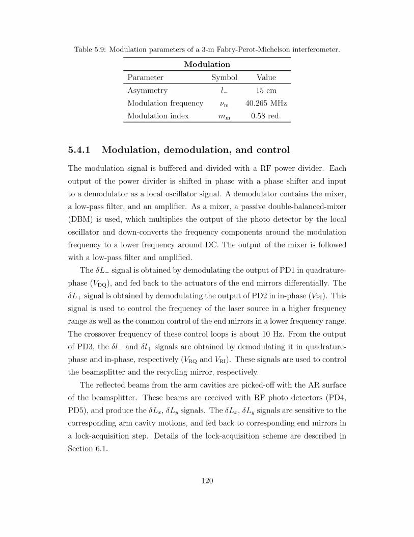
Table 5.9: Modulation parameters of a 3-m Fabry-Perot-Michelson interferometer.
Modulation
Parameter Symbol Value
Asymmetry l− 15 cm
Modulation frequency νm 40.265 MHz
Modulation index mm 0.58 red.
5.4.1 Modulation, demodulation, and control
The modulation signal is buffered and divided with a RF power divider. Each
output of the power divider is shifted in phase with a phase shifter and input
to a demodulator as a local oscillator signal. A demodulator contains the mixer,
a low-pass filter, and an amplifier. As a mixer, a passive double-balanced-mixer
(DBM) is used, which multiplies the output of the photo detector by the local
oscillator and down-converts the frequency components around the modulation
frequency to a lower frequency around DC. The output of the mixer is followed
with a low-pass filter and amplified.
The δL− signal is obtained by demodulating the output of PD1 in quadrature-
phase (VDQ), and fed back to the actuators of the end mirrors differentially. The
δL+ signal is obtained by demodulating the output of PD2 in in-phase (VPI). This
signal is used to control the frequency of the laser source in a higher frequency
range as well as the common control of the end mirrors in a lower frequency range.
The crossover frequency of these control loops is about 10 Hz. From the output
of PD3, the δl− and δl+ signals are obtained by demodulating it in quadrature-
phase and in-phase, respectively (VRQ and VRI). These signals are used to control
the beamsplitter and the recycling mirror, respectively.
The reflected beams from the arm cavities are picked-off with the AR surface
of the beamsplitter. These beams are received with RF photo detectors (PD4,
PD5), and produce the δLx, δLy signals. The δLx, δLy signals are sensitive to the
corresponding arm cavity motions, and fed back to corresponding end mirrors in
a lock-acquisition step. Details of the lock-acquisition scheme are described in
Section 6.1.
120

37 38 39 40 41 42 430.1
0.2
0.3
0.40.50.60.70.80.9
1
Frequency [MHz]
Mod
ulat
ion
inde
x [
rad]
Figure 5.14: Measured frequency response of the phase modulator. The
center frequency of the resonance is 39.88 MHz and a Q-value is 42.5.
5.4.2 Oscillator
The RF signal for phase modulation and demodulation is generated by a func-
tion synthesizer. The modulation frequency is set to be 40.265 MHz, which
is adjusted to satisfy the resonant condition of the RF sidebands with the recy-
cling cavity. The modulation signal of 10 Vpp from a function synthesizer (SONY
TEKTRONIX Inc., model AFG2020) is applied to the phase modulator. This RF
modulation signal is buffered by a power divider and distributed to the demod-
ulators as local oscillators. The phase of each local oscillator signal is adjusted
with a phase shifter so as to minimize the unnecessary signals.
5.4.3 Phase modulator
In order to control and operate the interferometer, the input laser beam is phase-
modulated in front of the interferometer. The modulation frequency is usually
set over about 10 MHz, where the intensity noise of the laser source is below
the shot noise level. The phase modulation around RF frequency is realized with
an electro-optic-modulator (EOM). We use a resonant-type EOM (NEW FOCUS
Inc., model 4003); the electro-optic crystal (LiTaO3) is combined with an inductor
to form a resonant circuit, resulting in a high modulation index with a small input
voltage. Figure 5.14 and 5.15 show the measured performance of the EOM. The
121
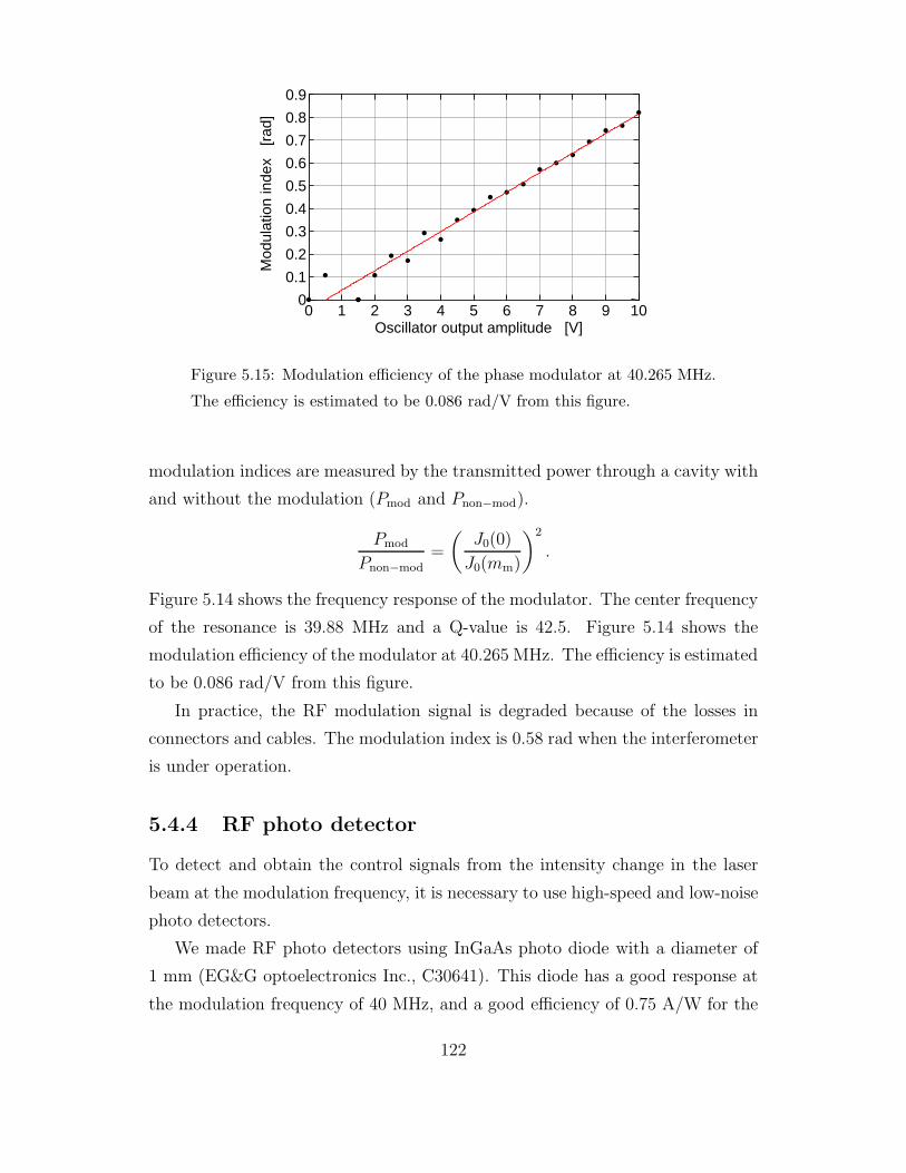
0 1 2 3 4 5 6 7 8 9 100
0.1
0.2
0.3
0.4
0.5
0.6
0.7
0.8
0.9
Oscillator output amplitude [V]
Mod
ulat
ion
inde
x [
rad]
Figure 5.15: Modulation efficiency of the phase modulator at 40.265 MHz.
The efficiency is estimated to be 0.086 rad/V from this figure.
modulation indices are measured by the transmitted power through a cavity with
and without the modulation (Pmod and Pnon−mod).
Pmod
Pnon−mod=
(J0(0)
J0(mm)
)2
.
Figure 5.14 shows the frequency response of the modulator. The center frequency
of the resonance is 39.88 MHz and a Q-value is 42.5. Figure 5.14 shows the
modulation efficiency of the modulator at 40.265 MHz. The efficiency is estimated
to be 0.086 rad/V from this figure.
In practice, the RF modulation signal is degraded because of the losses in
connectors and cables. The modulation index is 0.58 rad when the interferometer
is under operation.
5.4.4 RF photo detector
To detect and obtain the control signals from the intensity change in the laser
beam at the modulation frequency, it is necessary to use high-speed and low-noise
photo detectors.
We made RF photo detectors using InGaAs photo diode with a diameter of
1 mm (EG&G optoelectronics Inc., C30641). This diode has a good response at
the modulation frequency of 40 MHz, and a good efficiency of 0.75 A/W for the
122
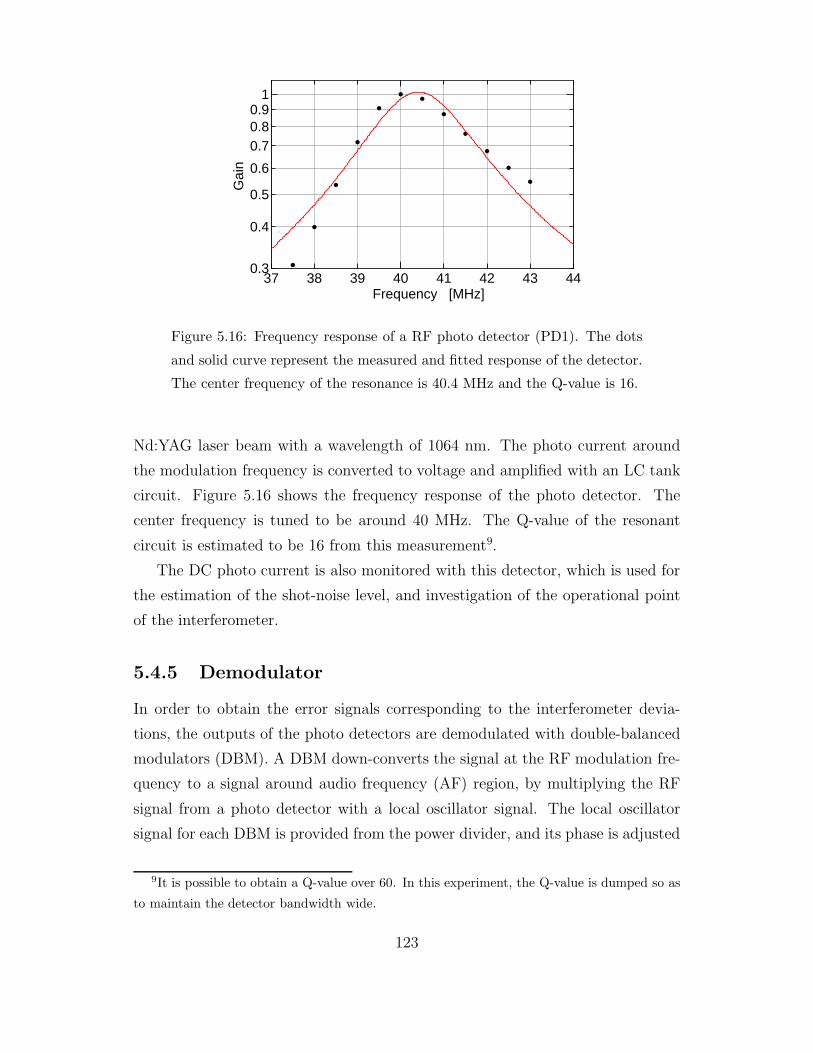
37 38 39 40 41 42 43 440.3
0.4
0.5
0.6
0.70.80.9
1
Frequency [MHz]
Gai
n
Figure 5.16: Frequency response of a RF photo detector (PD1). The dots
and solid curve represent the measured and fitted response of the detector.
The center frequency of the resonance is 40.4 MHz and the Q-value is 16.
Nd:YAG laser beam with a wavelength of 1064 nm. The photo current around
the modulation frequency is converted to voltage and amplified with an LC tank
circuit. Figure 5.16 shows the frequency response of the photo detector. The
center frequency is tuned to be around 40 MHz. The Q-value of the resonant
circuit is estimated to be 16 from this measurement9.
The DC photo current is also monitored with this detector, which is used for
the estimation of the shot-noise level, and investigation of the operational point
of the interferometer.
5.4.5 Demodulator
In order to obtain the error signals corresponding to the interferometer devia-
tions, the outputs of the photo detectors are demodulated with double-balanced
modulators (DBM). A DBM down-converts the signal at the RF modulation fre-
quency to a signal around audio frequency (AF) region, by multiplying the RF
signal from a photo detector with a local oscillator signal. The local oscillator
signal for each DBM is provided from the power divider, and its phase is adjusted
9It is possible to obtain a Q-value over 60. In this experiment, the Q-value is dumped so as
to maintain the detector bandwidth wide.
123

Table 5.10: Gain and noise of the demodulation systems. The gain of each
demodulation system is attenuated properly to avoid the saturation of RF
signal.
Demodulation
Signal Control Beam port PD Phase gdet [Ω] idet [mA]
VDQ δL− Detection PD1 Q 7.1 × 10³ 0.26
VRQ δl− Reflection PD3 Q 1.4 × 10⁴ 0.30
VPI δL+ Pick off PD2 I 2.1 × 10⁴ 0.22
VRI δl+ Reflection PD3 I 1.4 × 10⁴ 0.23
with a phase modulator. The output of a DBM is processed with a low-pass filter
to reject the up-converted signal and the leaking RF signal at the modulation
frequency and its harmonics. The low-pass filter is followed by a buffer amplifier.
The noise performance of the modulation-demodulation system is measured
by changing the input laser power on the photo detector (Fig. 5.17). The detection
system noise is described by the corresponding photocurrent. The relation of the
noise level and the photocurrent is written as Eq. (4.23)
Vdet = gdet
√e(iDC + idet) [V/
√Hz], (5.1)
where iDC is the DC photocurrent, gdet is the total demodulation gain (the con-
version ratio of RF photocurrent to the error signal), and idet is the dark current
corresponding to the noise of the demodulation system. When the input power is
high enough (iDC > idet), the floor level of the error signal is dominated by shot
noise, which is proportional to the square-root of the photocurrent. On the other
hand, when the input power is small (iDC < idet), the noise level is determined
by the noise of the detection system. The gain and noise of each demodulation
system is summarized in Table 5.10.
124

10–5 10–4 10–34e–08
5e–08
6e–087e–088e–089e–081e–07
2e–07
Noi
se le
vel
[V/H
z1/2 ]
Photocurrent [A]
idet
Figure 5.17: Measured noise level of the demodulated signal for δL− in
a function of photocurrent. Dots and solid curve represent the measured
and fitted noise levels, respectively. The correspond noise current of the
demodulation system (idet) is 0.26 mA.
5.5 Devices for monitor and measurement
5.5.1 AF photo detector
Besides the RF photo detector, photo detectors are placed to monitor powers of
laser beams from the interferometer. The power on the beamsplitter is monitored
with PD6 detecting the reflected beam on the AR surface of the beamsplitter.
The transmitted beams through the arm cavities are monitored with PD7 and
PD8. The incident laser power into the interferometer is monitored with PD9
placed on the input laser table.
5.5.2 Intensity modulator
An acousto-optic-modulator (AOM) placed in the input laser table is used to
modulate the intensity of the input beam. The effect of intensity noise is esti-
mated by modulating the input laser power.
The input laser beam into the interferometer is picked off by a partial mirror
(a reflectivity of about 10%), and its intensity noise is monitored with a photo
detector (PD9). The intensity of the input laser beam can be stabilized by feeding
125
back the output of PD9 to the AOM after filtering. However, we do not use this
intensity stabilization system because the intensity noise of the input beam does
not affect the current sensitivity of the interferometer (Section 6.4).
5.5.3 Optical spectrum analyzer
The transmissivity of the pick-off of the interferometer is adjusted so that the
signals from the reflection port are insensitive to the δL+ deviation. This condi-
tion is described as rrec1 = 0; no first-order sidebands are reflected back to the
laser source (Chapter 4). We monitor the power of the sidebands at the reflection
port with an optical spectrum analyzer in order to adjust and investigate the
signal-separation scheme.
The power of the carrier and sidebands are monitored with a Super Cav-
ity (NEWPORT Inc., model SR-100), which has the frequency resolution about
1 MHz.
5.6 Vacuum system
The main part of the interferometer is housed in a vacuum system in order to
avoid the effects of air fluctuation and sound noise (Fig. 5.18). The vacuum
system is comprised of a scroll pump and four vacuum tanks connected with
vacuum pipes with bellows. The diameter of the center and end tanks is 1 m,
and that of the recycling mirror tank is 70 cm. The vacuum pipes have a diameter
of 18 cm. The system is evacuated with a scroll pump connected to the center
tank. During operation of the interferometer, the pump is turned off to avoid the
vibration noises. The vacuum system keeps a pressure of about a few Torr with
the pump stopped.
The laser beam from the laser table is introduced in the vacuum system
through a window plate attached on the flange of the recycling mirror tank. Each
tank has connectors for input to actuators and outputs of the photo detectors.
126

1600 6503000
1260160 160650 6065060650500 100350
350
5600
500
Recycling mirror tank Center tank End tank 1
End tank 2
GV GV
GV
GV
B B
B
B
B
Pipe support
Pipe support
Window plate
Figure 5.18: Vacuum system of the 3-m Fabry-Perot-Michelson interferom-
eter. The vacuum system is comprised of a scroll pump and four vacuum
tanks connected with vacuum pipes, gate valves (GV), and bellows (B).
127
Chapter 6
Experiment
With the 3-m prototype interferometer, we have developed the control system for
a power-recycled interferometer. The experiment contains three topics. The first
topic is the lock-acquisition and operation of this prototype interferometer with
power recycling [32]. Since power recycling was not demonstrated in a Fabry-
Perot-Michelson interferometer with suspended mirrors before this research, it
was quite significant to investigate the lock acquisition process experimentally.
The second topic of this research is to test the signal-separation scheme for the
control of a power-recycled Fabry-Perot-Michelson interferometer [33]. The third
topic of this research is to estimate the effect of noise sources in the prototype
interferometer. The role of the control system is to maintain the stability, and
at the same time, sensitivity of the interferometer. Thus, the control system of
the 3-m prototype interferometer is designed not to degrade the sensitivity of the
interferometer.
In this Chapter, we describe the results of the power recycling experiments
on the 3-m prototype interferometer.
• Lock acquisition. Correlation diagram. Lock acquisition schemes: a
guide locking scheme and an automatic locking scheme.
• Operation with power recycling. Evaluations of the power-recycled
interferometer: power recycling gain, stability of the interferometer.
• Signal separation. Realization of the signal-separation scheme.
128
• Sensitivity of the interferometer. Displacement noise level and evalu-
ation of noise sources.
6.1 Lock acquisition
With frontal modulation, each control signal is linear to the motion in the cor-
responding degree of freedom only when the positions of the optical components
of the interferometer are near to the operational point. Thus, it is not a simple
problem to lock the interferometer from an uncontrolled state, particularly in an
interferometer with suspended optical components and a complex optical config-
uration. In a power-recycled Fabry-Perot-Michelson interferometer, four degrees
of freedom must be locked and kept at the operational point.
In the experiment of the 3-m prototype interferometer, we use two lock-
acquisition schemes; a guide locking scheme and an automatic locking scheme.
In the guide locking scheme, the interferometer is locked at the operational point
with auxiliary control loops. The auxiliary control signals are extracted from the
reflected beams from arm cavities. The automatic locking scheme is the simplest
way to lock the interferometer; the interferometer is locked by just closing all
of the longitudinal control loops. The process of the automatic lock has been
analyzed with a computer simulation by the LIGO group [75].
6.1.1 Correlation diagram
Here we show correlation diagram of the light power to see the operational status
of a power-recycled interferometer. Since the detection port is neither maxim
nor minimum at the operational point in a power-recycled interferometer, it is
impossible to confirm whether the interferometer is locked correctly by monitoring
the power only at the detection port. In order to confirm the operational point
of the interferometer, we monitor the light power on the beam splitter (PBS)
and the power at the detection port (Pdet), and the transmitted power through
the arm cavities1. The powers PBS and Pdet are simultaneously monitored by an
1The power on the beamsplitter PBS is monitored with PD9, detecting the reflected beam
on the AR surface of the beam splitter. The power at the detection port Pdet is monitored with
the DC output of PD1.
129

0 1 2 30
0.2
0.4
Power on the beam splitter
Det
ectio
n po
rt p
ower operational point
BS motion
RM motion
Optimal
Figure 6.1: Correlation diagram of the light power. In a power-recycled
interferometer, the operational point moves in the region bounded by an
elliptic curve and a line.
oscilloscope in X-Y mode; the X and Y axes are set to display PBS and Pdet,
respectively. The operational point is determined from the position of the spot,
and the motions of the mirrors are determined from the locus on the oscilloscope.
This locus is called a correlation diagram of the light power2 [26].
Figure 6.1 shows a correlation diagram of the light power. The horizontal and
vertical axises are proportional to PBS and Pdet, respectively. The horizontal axis
is normalized so that the power on the beam splitter without recycling mirror
should be unity; this value represents the power gain on the beam splitter. In a
power-recycled interferometer, the correlation point moves in the region bounded
by an elliptic curve and a line3. The sensitivity of an power-recycled interfer-
ometer is the best when the interference fringe is dark (φ− = 0) and the power
recycling cavity is resonant with the incident laser beam (φ+ = 0). Under these
conditions, the power on the beam splitter is maximized. When the recycling
mirror deviates from this optimal operational point, the power in the recycling
cavity decreases; the spot moves along the boundary line in the correlation di-
agram. On the other hand, when the beam splitter deviates from this optimal
2The correlation diagram described in this thesis is a little different from that in the reference
[26]; the reflected power from the interferometer was used for the horizontal axis.3Here, we assume the arm cavities are kept resonant with the incident laser beam.
130

0
1
2
3
0
1
2
3
0
1
2
3
0 1 2 3 4 50
1
2
3
Time [sec]
x–ar
my–
arm
BS
Det
ectio
n po
rt
B
C
A
Figure 6.2: Power change in the guide lock acquisition sequence. A: Both
arms cavities are locked independently with δLx and δLy signals. B: Re-
cycling cavity is locked with the δl+ signal. C: Beam-splitter is locked; all
degrees of freedom are locked.
operational point, the power leaks to the detection port; the point moves along
the elliptic boundary curve in the correlation diagram.
6.1.2 Guide locking scheme
One of the problems with lock acquisition is that the control signals are easily
affected by the misalignment of the interferometer and misadjustment of demod-
ulation phases; it is not easy to adjust under unlocked state. The point of guide
locking scheme is to use signals which are less affected by the motions in other
degrees of freedom of the interferometer, misalignment, and misadjustment of the
demodulation phases. Since the noise level of the auxiliary controls signal is not
good, the control system is switched to the final one step by step (Fig. 6.2 to
131
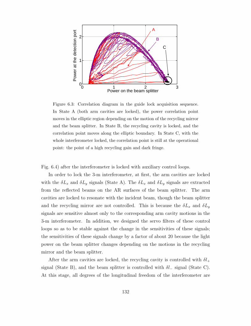
0 1 2 30
1
2
Power on the beam splitter
Pow
er a
t the
det
ectio
n po
rt A
B
C
Figure 6.3: Correlation diagram in the guide lock acquisition sequence.
In State A (both arm cavities are locked), the power correlation point
moves in the elliptic region depending on the motion of the recycling mirror
and the beam splitter. In State B, the recycling cavity is locked, and the
correlation point moves along the elliptic boundary. In State C, with the
whole interferometer locked, the correlation point is still at the operational
point: the point of a high recycling gain and dark fringe.
Fig. 6.4) after the interferometer is locked with auxiliary control loops.
In order to lock the 3-m interferometer, at first, the arm cavities are locked
with the δLx and δLy signals (State A). The δLx and δLy signals are extracted
from the reflected beams on the AR surfaces of the beam splitter. The arm
cavities are locked to resonate with the incident beam, though the beam splitter
and the recycling mirror are not controlled. This is because the δLx and δLy
signals are sensitive almost only to the corresponding arm cavity motions in the
3-m interferometer. In addition, we designed the servo filters of these control
loops so as to be stable against the change in the sensitivities of these signals;
the sensitivities of these signals change by a factor of about 20 because the light
power on the beam splitter changes depending on the motions in the recycling
mirror and the beam splitter.
After the arm cavities are locked, the recycling cavity is controlled with δl+
signal (State B), and the beam splitter is controlled with δl− signal (State C).
At this stage, all degrees of the longitudinal freedom of the interferometer are
132
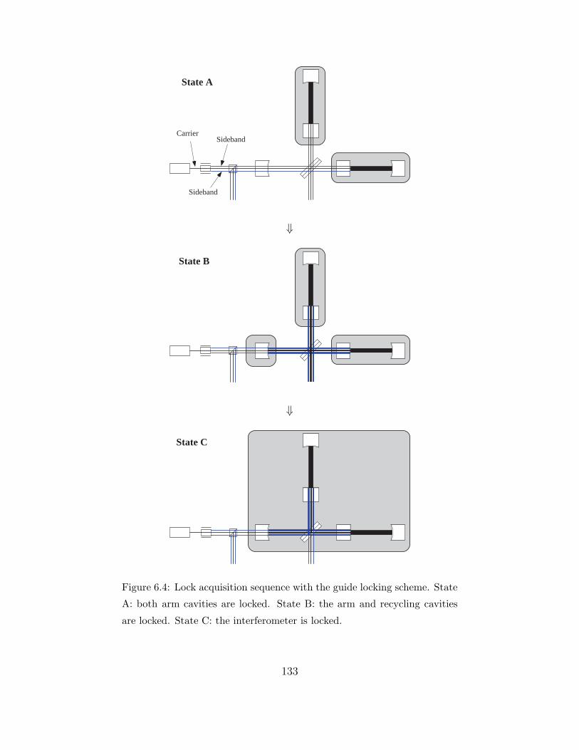
State A
CarrierSideband
Sideband
⇓
State B
⇓
State C
Figure 6.4: Lock acquisition sequence with the guide locking scheme. State
A: both arm cavities are locked. State B: the arm and recycling cavities
are locked. State C: the interferometer is locked.
133
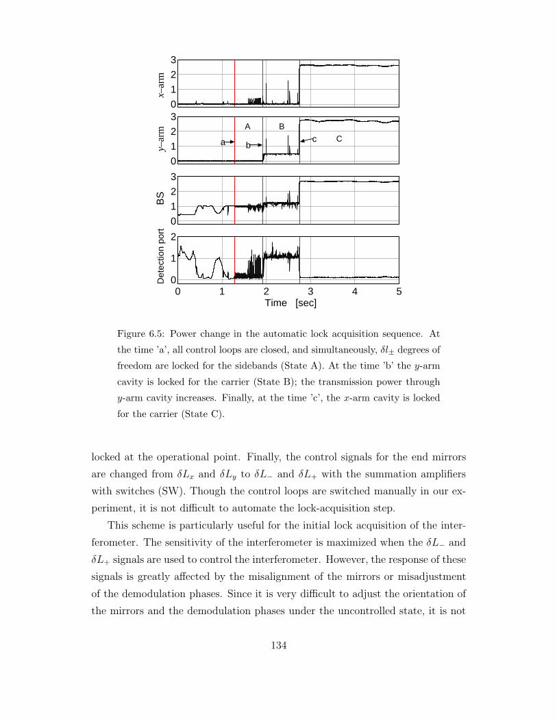
0
1
2
3
0
1
2
3
0
1
2
3
0 1 2 3 4 50
1
2
Time [sec]
x–ar
my–
arm
BS
Det
ectio
n po
rt
B
C
A
a bc
Figure 6.5: Power change in the automatic lock acquisition sequence. At
the time ’a’, all control loops are closed, and simultaneously, δl± degrees of
freedom are locked for the sidebands (State A). At the time ’b’ the y-arm
cavity is locked for the carrier (State B); the transmission power through
y-arm cavity increases. Finally, at the time ’c’, the x-arm cavity is locked
for the carrier (State C).
locked at the operational point. Finally, the control signals for the end mirrors
are changed from δLx and δLy to δL− and δL+ with the summation amplifiers
with switches (SW). Though the control loops are switched manually in our ex-
periment, it is not difficult to automate the lock-acquisition step.
This scheme is particularly useful for the initial lock acquisition of the inter-
ferometer. The sensitivity of the interferometer is maximized when the δL− and
δL+ signals are used to control the interferometer. However, the response of these
signals is greatly affected by the misalignment of the mirrors or misadjustment
of the demodulation phases. Since it is very difficult to adjust the orientation of
the mirrors and the demodulation phases under the uncontrolled state, it is not
134

0 1 2 30
1
2
C
A
B
Power on the beam splitter
Pow
er a
t the
det
ectio
n po
rt
Figure 6.6: Correlation diagram in the automatic lock acquisition sequence.
At State A, the detection port gets dark and the laser power on the beam
splitter increases a little. At State B, the interference fringe turns to bright.
Finally, all of the four degrees of freedom are locked at the operational point
(State C). The interference fringe turns to dark at the detection port, and
the laser power on the beam splitter increases.
easy to use the δL− and δL+ signals for the initial lock acquisition of the inter-
ferometer. The lock-acquisition scheme with the δLxand δLy signals is tolerant
against the initial misalignment of the mirrors or misadjustment of the demodula-
tion phases. By locking the interferometer with the auxiliary control loops (δLx,
δLy) together with the δl− and δl+ control loops, it is possible to finely align the
orientation of the mirrors of the interferometer to have a better contrast, a higher
recycling gain, and a higher transmissivity through the Fabry-Perot arm cavities.
The demodulation phase for each signal is also finely adjusted so as to minimize
the unnecessary signals.
6.1.3 Automatic locking scheme
Once the interferometer and demodulation phases are well adjusted, the interfer-
ometer is locked by just closing the δL−, δL+, δl− and δl+ control loops without
auxiliary control loops. This process has been analyzed with a computer simu-
lation by the LIGO group [75]. Figure 6.5 to Fig. 6.7 shows the automatic lock
acquisition sequence observed in the 3-m prototype interferometer.
135
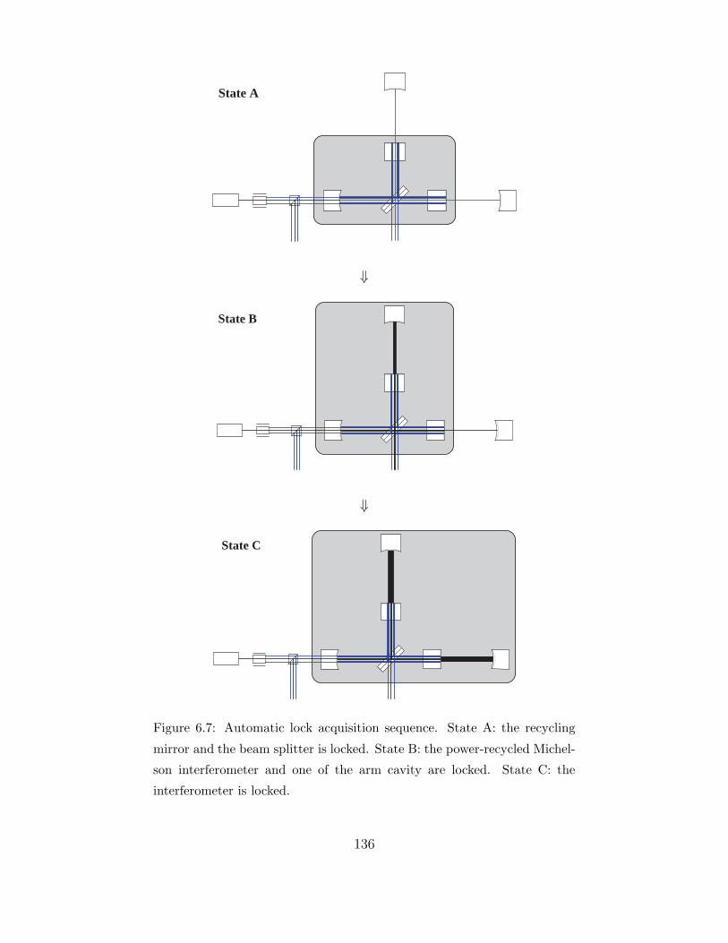
State A
⇓
State B
⇓
State C
Figure 6.7: Automatic lock acquisition sequence. State A: the recycling
mirror and the beam splitter is locked. State B: the power-recycled Michel-
son interferometer and one of the arm cavity are locked. State C: the
interferometer is locked.
136

Table 6.1: Table of power gains. The measured gains are in a good agree-
ment with calculated ones.
Power gain
Measured Calculated
Power recycling gain G0 2.4 2.5
Power gain on BS GBS 2.6 2.6
In this lock acquisition sequence, at first, the δl± degrees of freedom are locked
(State A). At this state, the sidebands resonate with the power-recycled Michelson
interferometer, while the carrier is anti-resonant with the interferometer. The
detection port becomes dark and the laser power on the beam splitter increases
in some extent because of the power gain of the sidebands. Next, one of the arm
cavities is locked (State B); the carrier resonates with one of the arm cavities
and with the recycling cavity. At this state, the interference fringe turns to
bright; the carrier beams from two arms of the Michelson interferometer interfere
constructively at the detection port. This is because the phase of the carrier
reflected by arm cavity differs by π under resonant and anti-resonant conditions.
At last, the carrier beam resonates with another arm cavity (State C); all of
the four degrees of freedom (δL± and δl±) are controlled and the interferometer
is locked at the operational point. The interference fringe turns to dark at the
detection port, and the laser power on the beam splitter increases.
Typically, the lock is acquired within a few second with the automatic locking
sequence when the interferometer is well-adjusted. However, this scheme does
not work well when the orientation of the mirrors and the demodulation phases
are not well adjusted. In this case, we adjust the interferometer locking the
interferometer with the guide locking scheme.
6.2 Operation with power recycling
The 3-m prototype interferometer is operated very stably with power recycling.
In this Section, we evaluate the power-recycled interferometer: a recycling gain,
stability of the operation, control loops, calibration of the error signals, residual
137

70 80 90 100
2
3
4
Transmissivity of the pick–off mirror [%]
Pow
er g
ain
on th
e be
am s
plitt
er
Figure 6.8: Power gain on the beam splitter as a function of the trans-
missivity of the pick-off. The dots are measured power gains on the beam
splitter, and the solid curve is a calculated one.
RMS deviations around the operational point, and a signal gain.
6.2.1 Power-recycling gain
When the interferometer is power-recycled, the laser power in it increases by a
factor called power gain. The power gain is defined as the ratio of the power
with and without the recycling mirror. Especially, the power gain of the carrier
beam is called power recycling gain. Since it is impossible to remove the recycling
mirror keeping the interferometer in vacuum in our system, we estimate the power
gain from the ratio of the power with power recycling and the power with the
recycling mirror misaligned.
G =PPR
PNR= TR
PPR
Pmiss, (6.1)
where TR is the power transmissivity of the recycling mirror, and PPR, PNR, and
Pmiss are the power with power recycling, without the recycling mirror, and with
the recycling mirror misaligned, respectively.
We measured the power gain monitoring the laser power at three points; the
powers transmitted trough the arm cavities (PD7, PD8), and the power on the
138
beam splitter (PD9). Since the arm cavities transmit only the carrier beam,
the power gain of the transmitted beam represents the gain of the carrier, i.e.,
the power-recycling gain (G0). On the other hand, the laser beam on the beam
splitter is comprised of the carrier and the sidebands. Neglecting the higher-order
sidebands, the power gain on the beam splitter (GBS) is written as
GBS = J20 (mm)G0 + 2J2
1 (mm)G1, (6.2)
where J0(mm) and J1(mm) are Bessel functions, mm is the modulation index, and
G1 is the power gain of the sidebands.
Table 6.1 shows the measured power gains together with gains calculated
with the measured reflectivities and transmissivities of the optical components.
Power gain on the beam splitter is also shown in Fig. 6.8, as a function of the
transmissivity of the pick-off; the dots and the solid line are the measured and
calculated power gains. From Table 6.1 and Fig. 6.8, we see that the measured
gains are in a good agreement with calculated ones.
6.2.2 Stability of operation
Once locked, the interferometer is operated very stably. Figure 6.9 shows the
power fluctuations 3-m RFPMI measured in 160 minutes from 4:40 till 7:20 in
the morning.
The upper plot shows fluctuation of power gains. The vertical axis is normal-
ized to show the power gains due to the power recycling. The lower line shows
the power-recycling gain4. The upper line shows the power gain on the beam
splitter.
The lower plot of Fig. 6.9 shows the fluctuation of the dark fringe. The vertical
axis is normalized to represent the contrast. Contrast indicates the completeness
of the interference. The averaged contrast in this measurement is 98.5%. In
general, the contrast of a Michelson interferometer is defined by
C =Pmax − Pmin
Pmax + Pmin, (6.3)
4The lower line in Fig. 6.9 is measured by monitoring the transmitted beam through the
x-arm cavity (PD7). The measured recycling gain by y-arm cavity (PD8) shows almost the
same line.
139
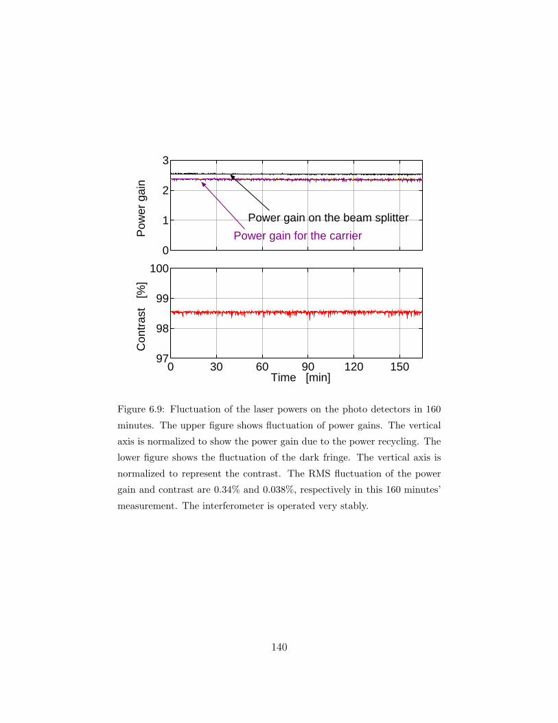
0
1
2
3
0 30 60 90 120 15097
98
99
100
Time [min]
Con
tras
t [%
]P
ower
gai
n
Power gain for the carrier
Power gain on the beam splitter
Figure 6.9: Fluctuation of the laser powers on the photo detectors in 160
minutes. The upper figure shows fluctuation of power gains. The vertical
axis is normalized to show the power gain due to the power recycling. The
lower figure shows the fluctuation of the dark fringe. The vertical axis is
normalized to represent the contrast. The RMS fluctuation of the power
gain and contrast are 0.34% and 0.038%, respectively in this 160 minutes’
measurement. The interferometer is operated very stably.
140

δL+
δL-
δl-
δl+
PD3
I
Buffer
Div
DBM
Q
PD1
PD2
Q
I
Filter
Sum
Diff
x End mirror
y End mirror
Beam splitter
Recycling mirror
Filter
Filter
Filter Coil driver
Buffer
Buffer
Buffer
PZT
PZT driver
Coil driver
Coil driver
Coil driver
Filter
Detection port
Reflection port
Pick-off port
Figure 6.10: Diagram of the control system of the 3-m Fabry-Perot-
Michelson interferometer. The δL− and δL+ signals are fed back to the
actuators of the end mirrors differentially and commonly, respectively. The
δL+ signal is also used to control the frequency of the laser source. The
δl− and δl+ signals are used to control the beam splitter and the recycling
mirror, respectively.
where Pmax and Pmin are maximum and minimum powers, i.e. bright and dark
fringe powers, respectively. These powers are usually measured by sweeping the
interference fringe. In a power-recycled Michelson interferometer, however, the
bright fringe power is not measured directly because the power incident on the
Michelson interferometer changes depending on the interference condition. Thus,
we estimated the bright fringe power with power recycling by
Pmax =1
TRGBSPmax,miss, (6.4)
where Pmax,miss is the bright fringe power with the recycling mirror misaligned.
The RMS fluctuation of the power gain and dark fringe power are 0.34% and
2.6%, respectively in this 160 minutes’ measurement. The fluctuation of 2.6%
of the dark fringe power corresponds to the contrast fluctuation of 0.038%. The
interferometer is operated very stably.
141

δL− loop δl− loop
10–4
10–2
100
102
102 103 104 105–360
–180
0
Abs
.P
hase
[d
eg]
Frequency [Hz]
10–4
10–2
100
101 102 103–360
–270
–180
–90
0
Frequency [Hz]
Pha
se
[deg
]A
bs.
δL+ loop δl+ loop
100
102
104
100 101 102 103 104 105–360
–270
–180
–90
0
Frequency [Hz]
Pha
se
[deg
]A
bs.
Mass loopTotal loop
PZT loop
Total loop
Mass loopPZT loop
10–4
10–2
100
101 102 103 104 105–360
–270
–180
–90
0
Frequency [Hz]
Pha
se
[deg
]A
bs.
Figure 6.11: Bode diagrams of the control loops. The dots are the measured
open loop transfer functions, and the solid curves are calculated open loop
transfer functions from the response of the interferometer, the filter circuits,
and the actuators.
6.2.3 Control system
Four degrees of freedom have to be controlled to operate a power-recycled Fabry-
Perot-Michelson interferometer. In this experiment the four signals necessary
for the control are obtained by frontal modulation (Chapter 4), and fed back to
suitable actuators after processing through filters (Fig 6.10).
Figure 6.11 shows the bode diagrams of the measured open loop transfer
functions of these four control loops. The dots are the measured open loop transfer
functions, and the solid curves are calculated open loop transfer functions from
142
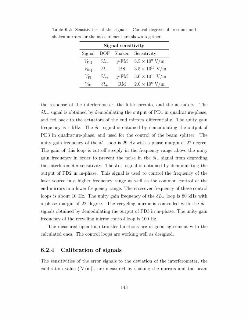
Table 6.2: Sensitivities of the signals. Control degrees of freedom and
shaken mirrors for the measurement are shown together.
Signal sensitivity
Signal DOF Shaken Sensitivity
VDQ δL− y-FM 8.5 × 10⁹ V/m
VRQ δl− BS 3.5 × 10¹⁰ V/m
VPI δL+ y-FM 3.6 × 10¹⁰ V/m
VRI δl+ RM 2.0 × 10⁸ V/m
the response of the interferometer, the filter circuits, and the actuators. The
δL− signal is obtained by demodulating the output of PD1 in quadrature-phase,
and fed back to the actuators of the end mirrors differentially. The unity gain
frequency is 1 kHz. The δl− signal is obtained by demodulating the output of
PD3 in quadrature-phase, and used for the control of the beam splitter. The
unity gain frequency of the δl− loop is 29 Hz with a phase margin of 27 degree.
The gain of this loop is cut off steeply in the frequency range above the unity
gain frequency in order to prevent the noise in the δl− signal from degrading
the interferometer sensitivity. The δL+ signal is obtained by demodulating the
output of PD2 in in-phase. This signal is used to control the frequency of the
laser source in a higher frequency range as well as the common control of the
end mirrors in a lower frequency range. The crossover frequency of these control
loops is about 10 Hz. The unity gain frequency of the δL+ loop is 80 kHz with
a phase margin of 22 degree. The recycling mirror is controlled with the δl+
signals obtained by demodulating the output of PD3 in in-phase. The unity gain
frequency of the recycling mirror control loop is 100 Hz.
The measured open loop transfer functions are in good agreement with the
calculated ones. The control loops are working well as designed.
6.2.4 Calibration of signals
The sensitivities of the error signals to the deviation of the interferometer, the
calibration value ([V/m]), are measured by shaking the mirrors and the beam
143

Table 6.3: Residual RMS deviations. These values are estimated from error
signals and intensity modulated peaks.
Residual RMS deviations
DOF Error signal Intensity modulation
δL− 2.2 × 10⁻¹¹ m 1.4 × 10⁻¹¹ m
δl− 1.3 × 10⁻⁹ m 2.6 × 10⁻⁹ m
δL+ 1.4 × 10⁻¹¹ m 5.5 × 10⁻¹⁰ m
δl+ 1.7 × 10⁻⁹ m 1.7 × 10⁻⁹ m
splitter. Since the calibration values are measured with the interferometer con-
trolled, it is necessary to consider the effect of the servo systems. The calibration
value with an open loop gain of Gopen is estimated as
∂V
∂X=
V × |1 + Gopen|X
, (6.5)
where V is the measured voltage of the error signal, and X is the displacement of
the shaken optical component. The displacement is estimated from the calibrated
value of the actuator (Table. 5.6) and shaking voltage into the actuator driver.
The measured sensitivities of the signals are summarized in Table 6.2. These
calibration values are also measured by shaking mirrors at 3 kHz5. The sensitivity
of the δL− and δL+ error signals have frequency dependence. The calculated cut-
off frequency of the signal is 106 kHz for δL− and 24 kHz for δL+.
6.2.5 Residual RMS deviations
Because of finite gains and offsets of the control system, the position of the
mirrors and the frequency of the laser source have residual deviations from the
ideal operational point. The residual RMS deviation is estimated from that of
the error signals using the calibration values.
The RMS deviations are also measured by modulating the intensity of the
input beam. The intensity modulation appears in the error signals coupling with5The calibration values are estimated from the open loop transfer functions. The frequency
response of these calibration values are in a good agreement with the measured value at 3 kHz
and calculated frequency response.
144
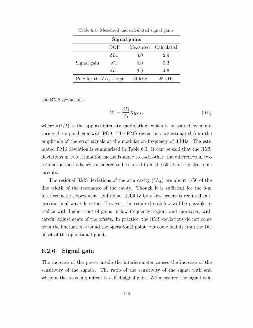
Table 6.4: Measured and calculated signal gains.
Signal gains
DOF Measured Calculated
δL− 3.0 2.9
Signal gain δl− 4.0 3.3
δL+ 6.9 4.6
Pole for the δL+ signal 24 kHz 25 kHz
the RMS deviations.
δV =δPl
PlXRMS, (6.6)
where δPl/Pl is the applied intensity modulation, which is measured by moni-
toring the input beam with PD9. The RMS deviations are estimated from the
amplitude of the error signals at the modulation frequency of 3 kHz. The esti-
mated RMS deviation is summarized in Table 6.3. It can be said that the RMS
deviations in two estimation methods agree to each other; the differences in two
estimation methods are considered to be caused from the offsets of the electronic
circuits.
The residual RMS deviations of the arm cavity (δL±) are about 1/50 of the
line width of the resonance of the cavity. Though it is sufficient for the 3-m
interferometer experiment, additional stability by a few orders is required in a
gravitational wave detector. However, the required stability will be possible to
realize with higher control gains in low frequency region, and moreover, with
careful adjustments of the offsets. In practice, the RMS deviations do not come
from the fluctuation around the operational point, but come mainly from the DC
offset of the operational point.
6.2.6 Signal gain
The increase of the power inside the interferometer causes the increase of the
sensitivity of the signals. The ratio of the sensitivity of the signal with and
without the recycling mirror is called signal gain. We measured the signal gain
145

δL− signal δl− signal
100
101
102 103 104 105–180
0
180
Abs
.P
hase
[de
g]
Frequency [Hz]
100
101
102 103–180
0
180
Abs
.P
hase
[d
eg]
Frequency [Hz]
δL+ signal
100
101
102
102 103 104 105–180
0
180
Abs
.P
hase
[d
eg]
Frequency [Hz]
Figure 6.12: The absolute value and phase of the signal gain. Dots and the
solid curves are the measured and fitted signal gains.
146

from open loop transfer functions6 with power recycling and with the recycling
mirror misaligned.
Gsig = TR
(Gopen
Gfilter
)PR(
Gopen
Gfilter
)miss
, (6.7)
where Gopen is the open loop transfer function, and Gfilter is the transfer function
of the filter circuit, the gain of which is adjusted in each configuration.
Figure 6.12 shows the measured signal gains. The upper-left figure shows
the signal gain of the δL− control signal, which is extracted from the detection
port. The signal gain for δL− is described as g0g1, the product of amplitude gains
for the carrier and the sidebands. The measured signal gain of 3.0 is in a good
agreement with the calculated value of 2.9. The frequency dependence of this
signal is not changed with and without power recycling; the signal gain has no
frequency dependence. The upper-right figure shows the signal gain of the δl−
control signal, which is extracted from the reflection port. The measured signal
gain of δl− is 4.0, and has no frequency dependence. The lower figure shows the
signal gain of the δL+ control signal, which is extracted from the pick-off port.
This signal gain is 6.9, and has a pole at 24 kHz. The signal gain for the δL+ has
a frequency dependence; the cut-off frequency shifts lower with power recycling
because the storage time of the δL+ signal in the interferometer increases.
The signal gains are also estimated from the calibration values of the signals
with and without power recycling. These signal gains are in good agreement with
the values estimated from the open loop transfer functions.
6.3 Signal separation
One of the problems on controlling a power-recycled Fabry-Perot-Michelson in-
terferometer is the extraction of the signal for the fluctuations of recycling cavity
length, the δl+ motion. In a conventional frontal modulation scheme, the δl+
information is mixed by a large δL+ information. However, with the signal sepa-
ration scheme described in Section 4.4, the VRI signal, the in-phase demodulated
6Note that the open loop transfer function is a product of the sensitivity of the control
signal, the transfer function of the electronic circuits and the that of the actuator.
147
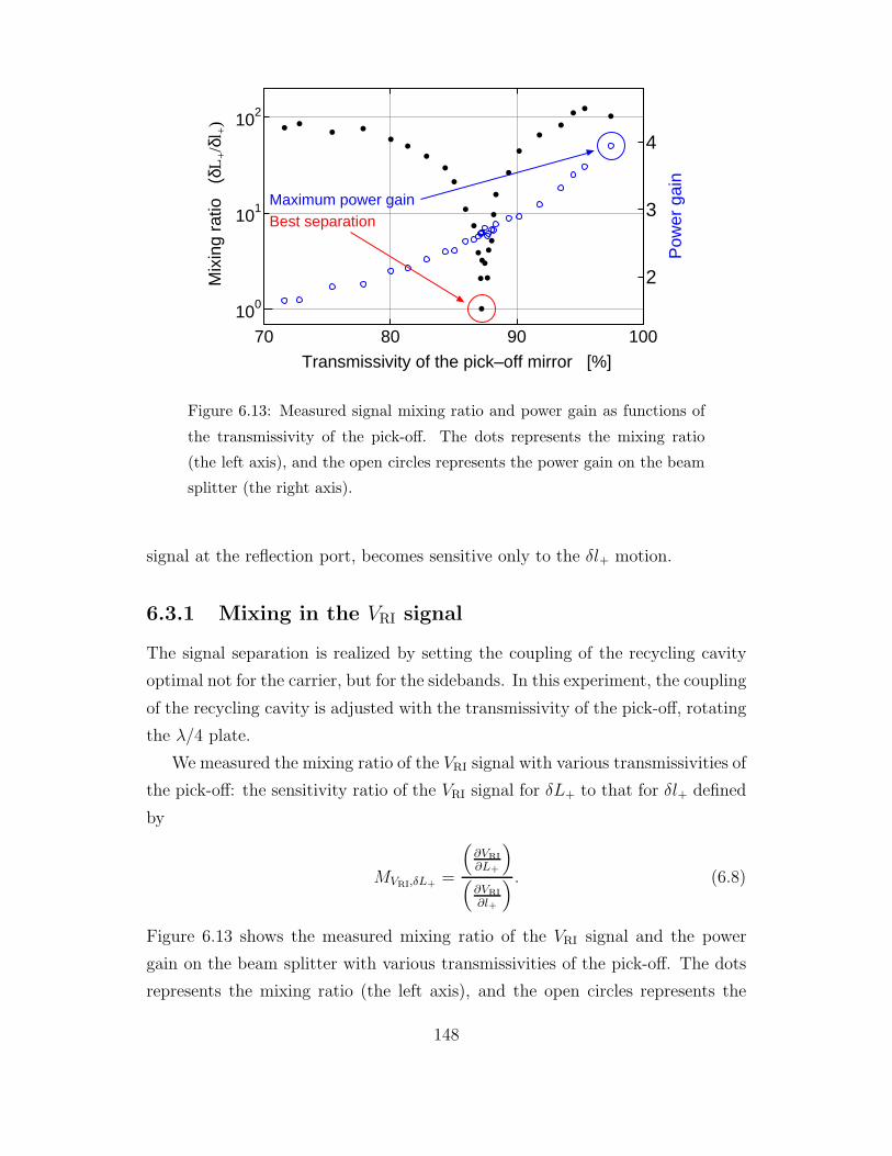
70 80 90 100100
101
102
2
3
4
Transmissivity of the pick–off mirror [%]
Mix
ing
ratio
(δ
L+/δ
l +)
Pow
er g
ain
Best separationMaximum power gain
Figure 6.13: Measured signal mixing ratio and power gain as functions of
the transmissivity of the pick-off. The dots represents the mixing ratio
(the left axis), and the open circles represents the power gain on the beam
splitter (the right axis).
signal at the reflection port, becomes sensitive only to the δl+ motion.
6.3.1 Mixing in the VRI signal
The signal separation is realized by setting the coupling of the recycling cavity
optimal not for the carrier, but for the sidebands. In this experiment, the coupling
of the recycling cavity is adjusted with the transmissivity of the pick-off, rotating
the λ/4 plate.
We measured the mixing ratio of the VRI signal with various transmissivities of
the pick-off: the sensitivity ratio of the VRI signal for δL+ to that for δl+ defined
by
MVRI,δL+ =
(∂VRI
∂L+
)(
∂VRI
∂l+
) . (6.8)
Figure 6.13 shows the measured mixing ratio of the VRI signal and the power
gain on the beam splitter with various transmissivities of the pick-off. The dots
represents the mixing ratio (the left axis), and the open circles represents the
148

Table 6.5: Measured signal sensitivity matrix without signal separation.
The transmissivity of the pick-off is 98%
Mixing ratio without signal separation
δL− δl− δL+ δl+
VDQ 1 7.4 × 10⁻³ 2.1 × 10⁻² 2.1 × 10⁻⁴
VRQ 1.6 1 13 3.7
VPI 0.10 2.4 × 10⁻² 1 3.4 × 10⁻²
VRI 0.12 0.73 130 1
power gain on the beam splitter (the right axis). The best mixing ratio of 1.01 is
obtained at the pick-off transmissivity of 87.2%. When the transmissivity is 97.4%
(the maximum value in this figure), the mixing ratio is 102. Thus, the mixing
ratio is improved by a factor of 100 with the adjustment of optical parameters.
As described above, the mixing ratio of δL+ to δl+ is about unity when the
transmissivity of the pick-off is optimized. This ratio is considered to be limited
by the residual motion of the interferometer as well as misadjustment of the trans-
missivity of the pick-off. The fluctuation of the reflectivity of the compound mir-
ror for the sidebands causes deviation from the optimal signal-separation point,
resulting in degradation of the signal-separation ratio. From the signal-mixing
measurement (Fig. 6.13), the mixing ratio is estimated to be
MVRI,δL+ ' 705 × ∆Rcom1. (6.9)
The measured RMS deviation in δl− is 2.6 × 10⁻⁹ m. This residual motion
corresponds to the fluctuation ∆Rcom1 = 9.3 × 10⁻⁴ (0.093%). The resultant
mixing ratio is 0.7, which is in good agreement with the measured mixing ratio.
A small drift of the signal-separation point is observed during the measure-
ment. However, it is possible to keep signal separation ratio around unity in a few
tens of minutes. The mixing ratio gets worse to about 3 in a few hours, probably
because of the drifts in the alignment of the interferometer.
149

Table 6.6: Measured signal sensitivity matrix with signal separation. The
transmissivity of the pick-off is 87%
Mixing ratio with signal separation
δL− δl− δL+ δl+
VDQ 1 7.4 × 10⁻³ 2.3 × 10⁻² 1.8 × 10⁻⁴
VRQ 0.12 1 2.21 7.2 × 10⁻²
VPI 1.7 × 10⁻² 0.18 1 0.81
VRI 0.47 0.80 1.4 1
6.3.2 Signal sensitivity matrix
Besides the signal mixing in the VRI signal described above, the signals mix one
another. The signal mixing ratio of the signal V is defined by
MV,δX =
(∂V∂X
)(∂V
∂Xcontrol
) , (6.10)
where X is one of four degrees of freedom to be controlled, and Xcontrol is the
controlled degree of freedom with the V signal7. Table 6.5 and 6.6 show the signal
sensitives without and with signal separation, respectively. The sensitivities were
measured at a frequency of 3 kHz. We see from these tables that the matrix is
well-diagonalized with signal separation. Without signal separation (Table 6.5),
the matrix has a large value of 130 in the MVRI,δL+ component. While this value
is decreases to 1.4 with signal separation (Table 6.6). In addition, note that the
mixing of δL+ in the VRQ signal, which is used for the δl− control, is improved
with signal separation. The δL+ information mixes easily into the VRQ signal
coupling with the misadjustment of the demodulation phase without the signal-
separation condition. On the other hand, since RF sidebands are absent at the
reflection port with the signal-separation scheme, δL+ becomes harder to appear
in the VRQ signal even if the demodulation phase is misadjusted some extent.
7The four signals and the four degrees of freedom are arranged so that the table would be
an unity matrix when no signal mixing is exist.
150
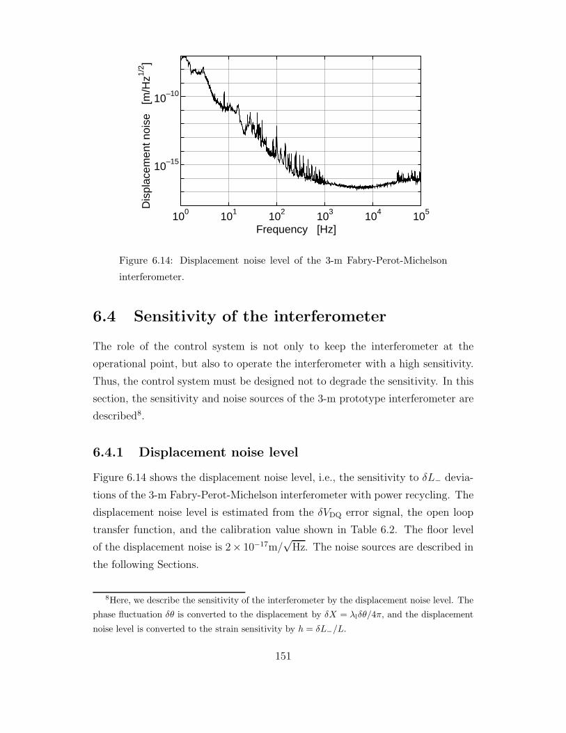
100 101 102 103 104 105
10–15
10–10
Frequency [Hz]
Dis
plac
emen
t noi
se
[m/H
z1/2 ]
Figure 6.14: Displacement noise level of the 3-m Fabry-Perot-Michelson
interferometer.
6.4 Sensitivity of the interferometer
The role of the control system is not only to keep the interferometer at the
operational point, but also to operate the interferometer with a high sensitivity.
Thus, the control system must be designed not to degrade the sensitivity. In this
section, the sensitivity and noise sources of the 3-m prototype interferometer are
described8.
6.4.1 Displacement noise level
Figure 6.14 shows the displacement noise level, i.e., the sensitivity to δL− devia-
tions of the 3-m Fabry-Perot-Michelson interferometer with power recycling. The
displacement noise level is estimated from the δVDQ error signal, the open loop
transfer function, and the calibration value shown in Table 6.2. The floor level
of the displacement noise is 2× 10⁻¹⁷m/√
Hz. The noise sources are described in
the following Sections.
8Here, we describe the sensitivity of the interferometer by the displacement noise level. The
phase fluctuation δθ is converted to the displacement by δX = λlδθ/4π, and the displacement
noise level is converted to the strain sensitivity by h = δL−/L.
151

101 102 103 104 10510–18
10–16
10–14
10–12
10–10
Frequency [Hz]
Dis
plac
emen
t noi
se
[m/H
z1/2 ]
Demodulation system noise
Shot noise
Figure 6.15: Shot-noise level and the demodulation noise level of the 3-m
Fabry-Perot-Michelson interferometer.
6.4.2 Estimation of noise level
Shot noise
Shot noise is one of the fundamental noise sources in a laser interferometric grav-
itational wave detector. The DC photo current on the photo detector (iDC)
produces a shot noise (ishot) described by
ishot =√
2eiDC. (6.11)
This shot-noise current is demodulated and appears in the error signal. The
averaged photo current at the detection port detector is measured to be 0.11 mA
when the interferometer is operated with power recycling. From this DC photo
current, the gain of the demodulation system, and the calibration value, the
shot noise level is estimated to be 3.5 × 10⁻¹⁸ [m/√
Hz]. The shot noise level is
shown in Fig. 6.15 together with the displacement noise level of the 3-m prototype
interferometer9.
In practice, the demodulation system has a noise represented by the corre-
sponding noise current idet, which is 0.26 mA for VDQ. Thus, the noise level is
9The shot noise level increases in a high frequency region because of the cutoff of the Fabry-
Perot arm cavity at 106 kHz.
152

100 101 102 103
10–16
10–12
10–8
Frequency [Hz]
Dis
plac
emen
t [m
/Hz1/
2 ]
Seismic motion
Figure 6.16: Seismic noise level of the 3-m Fabry-Perot-Michelson interfer-
ometer. The displacement noise level is limited by the seismic noise below
100 Hz.
dominated by the demodulation system noise rather than the shot noise. The
noise level of the demodulation system is also shown in Fig. 6.15. The total noise
level of the shot noise and demodulation system noise is calculated from Eq. (5.1),
which results in the displacement noise of 6.3 × 10⁻¹⁸ [m/√
Hz].
Seismic noise
Though the optical components are suspended and isolated from the seismic
motion, the sensitivity of the interferometer is still affected by the seismic noise
in a low frequency region. Figure 6.16 shows the seismic noise level together with
the displacement noise level of the 3-m prototype interferometer. The seismic
motion of a mirror is estimated from a measured ground motion and the seismic
isolation ratio of the suspension system (Fig. 5.6). The seismic noise level of
the interferometer is estimated by multiplying the motion of a mirror by√
4,
assuming that the motions of the four mirrors have no correlation10. We see that
10In Fig. 6.16, the displacement noise level is lower than the estimated seismic noise level.
This is probably because the motions of the mirrors of the interferometer have some correlation
in a low frequency region.
153

101 102 103 104 105
10–15
10–10
Frequency [Hz]
Dis
plac
emen
t noi
se
[m/H
z1/2 ]
Thermal noise (mass)
Thermal noise (violin)
Thermal noise (pendulum)
Figure 6.17: Thermal noise level of the 3-m Fabry-Perot-Michelson inter-
ferometer. The thermal noises do not affect the sensitivity of the interfer-
ometer except for the resonant frequency of the test mass (37 kHz).
the displacement noise level is limited by the seismic noise below 100 Hz from
Fig. 6.16.
Thermal noise
Thermal noise is the other fundamental noise source for an interferometric gravi-
tational wave detector. However, since the sensitivity of the 3-m prototype inter-
ferometer is not so high, the thermal noise level is lower than the sensitivity level
except for the resonant frequencies of the test mass and violin modes. Figure 6.17
shows the thermal noise level. The thermal noise of the mass is calculated only
for the lowest internal mode of the test mass, assuming the structure damping
model. The measured Q-values are 1,600 to 27,000 for four test masses. The
resonant frequency is 37 kHz, and an effective mass of 0.23 kg. The thermal noise
for the pendulum is calculated with a Q-value of 1000, a resonant frequency of
1.2 Hz, and an effective mass of 0.46 kg. The resonant frequency of the lowest
violin mode is calculated to be 250 Hz. The Q-value of the violin modes are
assumed to be 500.
154
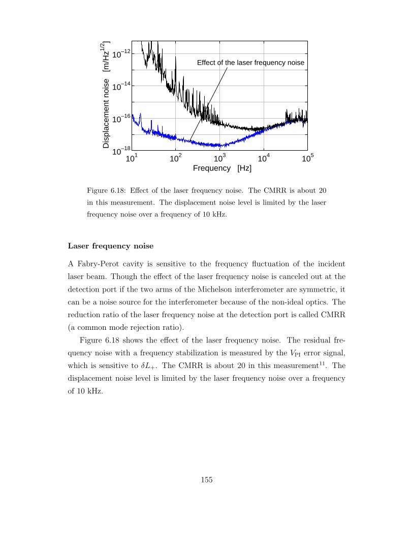
101 102 103 104 10510–18
10–16
10–14
10–12
Frequency [Hz]
Dis
plac
emen
t noi
se
[m/H
z1/2 ]
Effect of the laser frequency noise
Figure 6.18: Effect of the laser frequency noise. The CMRR is about 20
in this measurement. The displacement noise level is limited by the laser
frequency noise over a frequency of 10 kHz.
Laser frequency noise
A Fabry-Perot cavity is sensitive to the frequency fluctuation of the incident
laser beam. Though the effect of the laser frequency noise is canceled out at the
detection port if the two arms of the Michelson interferometer are symmetric, it
can be a noise source for the interferometer because of the non-ideal optics. The
reduction ratio of the laser frequency noise at the detection port is called CMRR
(a common mode rejection ratio).
Figure 6.18 shows the effect of the laser frequency noise. The residual fre-
quency noise with a frequency stabilization is measured by the VPI error signal,
which is sensitive to δL+. The CMRR is about 20 in this measurement11. The
displacement noise level is limited by the laser frequency noise over a frequency
of 10 kHz.
155
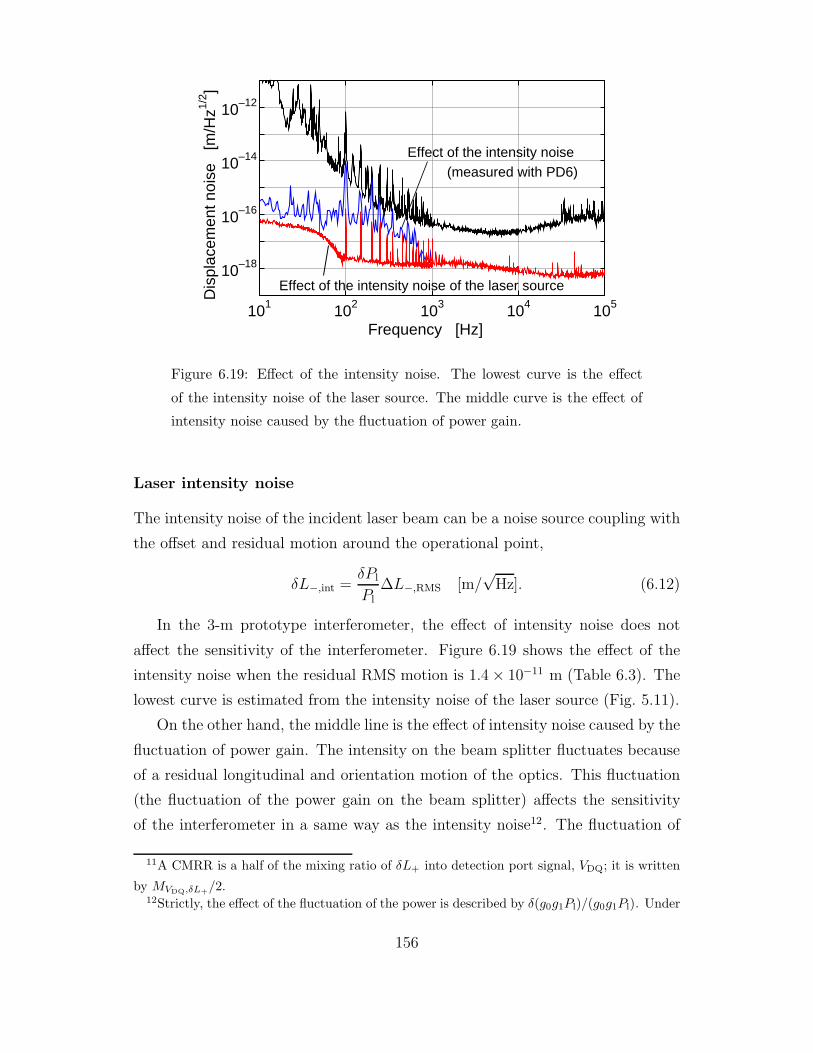
101 102 103 104 105
10–18
10–16
10–14
10–12
Frequency [Hz]
Dis
plac
emen
t noi
se
[m/H
z1/2 ]
Effect of the intensity noise
Effect of the intensity noise of the laser source
(measured with PD6)
Figure 6.19: Effect of the intensity noise. The lowest curve is the effect
of the intensity noise of the laser source. The middle curve is the effect of
intensity noise caused by the fluctuation of power gain.
Laser intensity noise
The intensity noise of the incident laser beam can be a noise source coupling with
the offset and residual motion around the operational point,
δL−,int =δPl
Pl
∆L−,RMS [m/√
Hz]. (6.12)
In the 3-m prototype interferometer, the effect of intensity noise does not
affect the sensitivity of the interferometer. Figure 6.19 shows the effect of the
intensity noise when the residual RMS motion is 1.4 × 10⁻¹¹ m (Table 6.3). The
lowest curve is estimated from the intensity noise of the laser source (Fig. 5.11).
On the other hand, the middle line is the effect of intensity noise caused by the
fluctuation of power gain. The intensity on the beam splitter fluctuates because
of a residual longitudinal and orientation motion of the optics. This fluctuation
(the fluctuation of the power gain on the beam splitter) affects the sensitivity
of the interferometer in a same way as the intensity noise12. The fluctuation of
11A CMRR is a half of the mixing ratio of δL+ into detection port signal, VDQ; it is written
by MVDQ,δL+/2.12Strictly, the effect of the fluctuation of the power is described by δ(g0g1Pl)/(g0g1Pl). Under
156
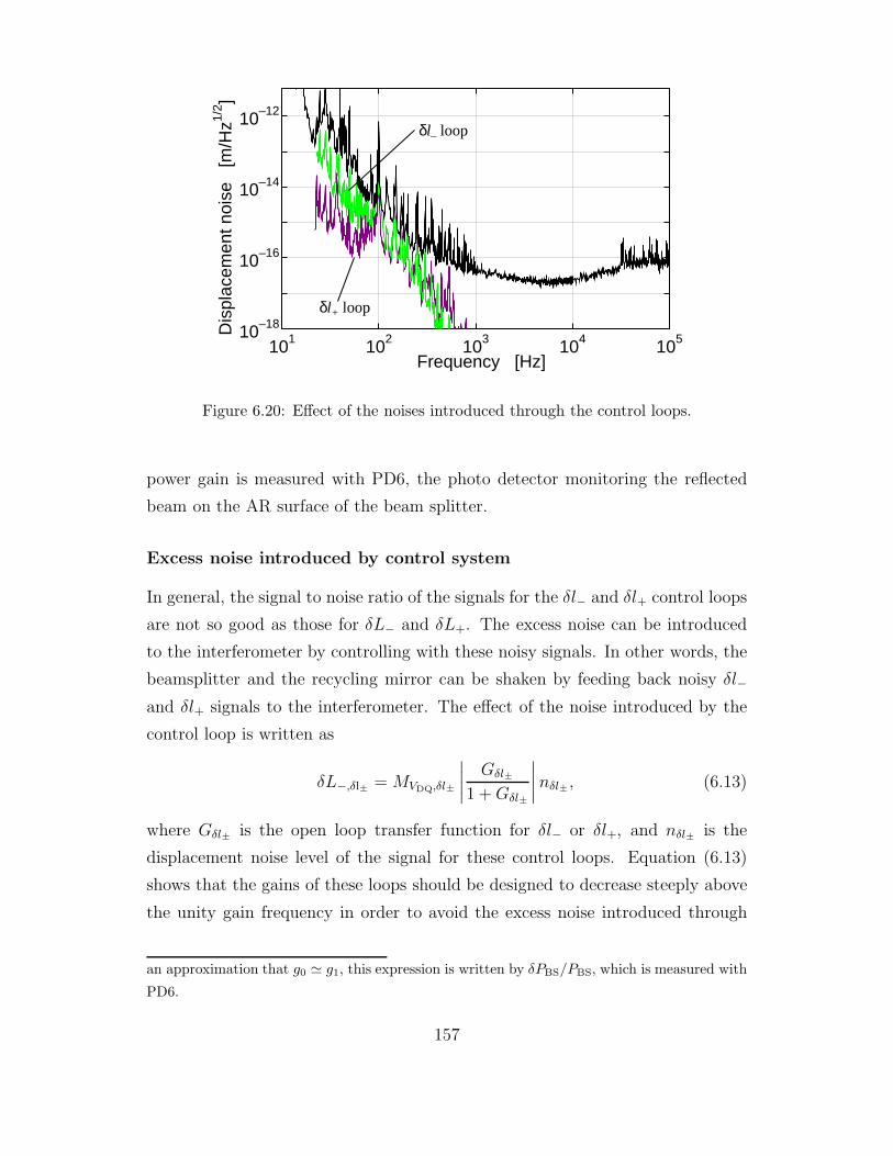
101 102 103 104 10510–18
10–16
10–14
10–12
Frequency [Hz]
Dis
plac
emen
t noi
se
[m/H
z1/2 ]
δl– loop
δl+ loop
Figure 6.20: Effect of the noises introduced through the control loops.
power gain is measured with PD6, the photo detector monitoring the reflected
beam on the AR surface of the beam splitter.
Excess noise introduced by control system
In general, the signal to noise ratio of the signals for the δl− and δl+ control loops
are not so good as those for δL− and δL+. The excess noise can be introduced
to the interferometer by controlling with these noisy signals. In other words, the
beamsplitter and the recycling mirror can be shaken by feeding back noisy δl−
and δl+ signals to the interferometer. The effect of the noise introduced by the
control loop is written as
δL−,δl± = MVDQ,δl±
∣∣∣∣ Gδl±
1 + Gδl±
∣∣∣∣nδl±, (6.13)
where Gδl± is the open loop transfer function for δl− or δl+, and nδl± is the
displacement noise level of the signal for these control loops. Equation (6.13)
shows that the gains of these loops should be designed to decrease steeply above
the unity gain frequency in order to avoid the excess noise introduced through
an approximation that g0 ' g1, this expression is written by δPBS/PBS, which is measured with
PD6.
157

101 102 103 104 105
10–18
10–16
10–14
10–12
Frequency [Hz]
Dis
plac
emen
t noi
se
[m/H
z1/2 ]
δL– filter
δl– filter
δL+ mass filter
δL+ PZT filterδl+ filter
Figure 6.21: Effect of the electronic noises of the control circuits. The noise
of δL− filter is limiting the sensitivity from 60 Hz to 200 Hz.
the control loops. In particular, a severe restriction is required for the δl− control
loop13.
The control loop for δl− is designed to decrease steeply above the unity gain
frequency in the 3-m interferometer. Thus, the excess noise introduced through
the control loop is reduced lower than the displacement noise level although the
control signals are affected not only by the shot noise but also by the intensity
noise, the laser frequency noise, the seismic noise, and so on. Though the control
loop for δl+ is not designed to cut off steeply, the excess noise does not affect the
sensitivity of the interferometer except for several resonant peaks14.
13In the 3-m prototype interferometer, the shot noise level for the δl− is 4.5× 10⁻¹⁵ m/√
Hz
and MVDQ,δl− = 7.4 × 10⁻³. Thus, the product of these is 3.3 × 10⁻¹⁷ m/√
Hz. Thus, the shot
noise of the δl− control signal can limit the displacement noise level without a proper design.
On the other hand, the shot noise level for δl+ is 7.7×10⁻¹⁶ m/√
Hz and MVDQ,δl+ = 1.8×10⁻⁴.
The product of these is 1.4 × 10⁻¹⁹ m/√
Hz. This noise level is much below the displacement
noise level of the 3-m prototype interferometer.14The noise in the δl+ error signal is introduced also into the δL+ signal through the control
loop. However, with the signal separation scheme, the requirement would not be severe because
the sensitivity for δl+ is high enough. However, if a high stability is required for the laser
frequency, or if the conventional frontal modulation scheme is used, the laser frequency stability
can be limited by the noise in the δl+ error signal.
158
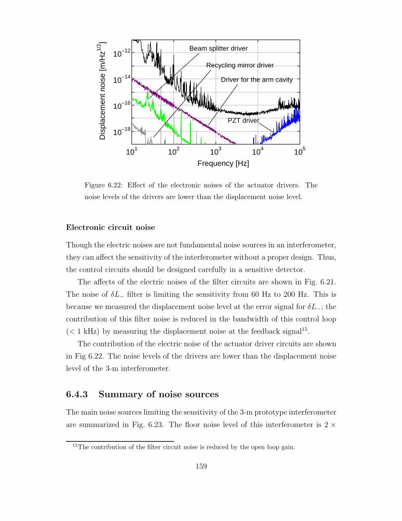
101 102 103 104 105
10–18
10–16
10–14
10–12
Frequency [Hz]
Dis
plac
emen
t noi
se [m
/Hz1/
2 ]
Driver for the arm cavity
Beam splitter driver
Recycling mirror driver
PZT driver
Figure 6.22: Effect of the electronic noises of the actuator drivers. The
noise levels of the drivers are lower than the displacement noise level.
Electronic circuit noise
Though the electric noises are not fundamental noise sources in an interferometer,
they can affect the sensitivity of the interferometer without a proper design. Thus,
the control circuits should be designed carefully in a sensitive detector.
The affects of the electric noises of the filter circuits are shown in Fig. 6.21.
The noise of δL− filter is limiting the sensitivity from 60 Hz to 200 Hz. This is
because we measured the displacement noise level at the error signal for δL−; the
contribution of this filter noise is reduced in the bandwidth of this control loop
(< 1 kHz) by measuring the displacement noise at the feedback signal15.
The contribution of the electric noise of the actuator driver circuits are shown
in Fig 6.22. The noise levels of the drivers are lower than the displacement noise
level of the 3-m interferometer.
6.4.3 Summary of noise sources
The main noise sources limiting the sensitivity of the 3-m prototype interferometer
are summarized in Fig. 6.23. The floor noise level of this interferometer is 2 ×
15The contribution of the filter circuit noise is reduced by the open loop gain.
159

101 102 103 104 10510–18
10–16
10–14
10–12
10–10
Frequency [Hz]
Dis
plac
emen
t noi
se
[m/H
z1/2 ]
Shot noise
Seismic noise
Laser frequency noise
Displacement noise level
Filter noise
Demodulation system noise
Figure 6.23: Estimated noise sources of the 3-m Fabry-Perot-Michelson
interferometer. In a lower frequency range, the sensitivity is limited by
the seismic noise (∼100 Hz) and the noise of the filter circuit (∼200 Hz).
In a high frequency range, the sensitivity is limited by the laser fre-
quency noise (10 kHz∼). The noise source in the middle frequency range
(200 Hz∼10 kHz) is not identified. One candidate for this noise is a thermal
noise at the bonding of the mirror.
160
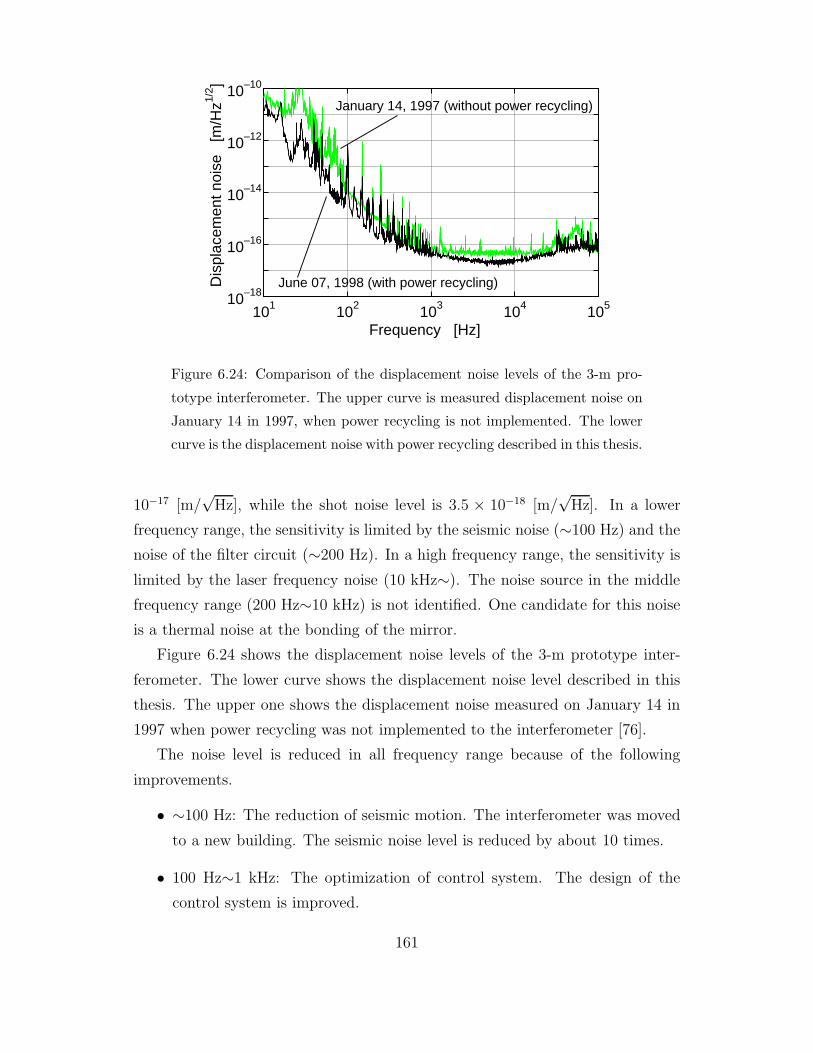
101 102 103 104 10510–18
10–16
10–14
10–12
10–10
Frequency [Hz]
Dis
plac
emen
t noi
se
[m/H
z1/2 ]
January 14, 1997 (without power recycling)
June 07, 1998 (with power recycling)
Figure 6.24: Comparison of the displacement noise levels of the 3-m pro-
totype interferometer. The upper curve is measured displacement noise on
January 14 in 1997, when power recycling is not implemented. The lower
curve is the displacement noise with power recycling described in this thesis.
10−17 [m/√
Hz], while the shot noise level is 3.5 × 10⁻¹⁸ [m/√
Hz]. In a lower
frequency range, the sensitivity is limited by the seismic noise (∼100 Hz) and the
noise of the filter circuit (∼200 Hz). In a high frequency range, the sensitivity is
limited by the laser frequency noise (10 kHz∼). The noise source in the middle
frequency range (200 Hz∼10 kHz) is not identified. One candidate for this noise
is a thermal noise at the bonding of the mirror.
Figure 6.24 shows the displacement noise levels of the 3-m prototype inter-
ferometer. The lower curve shows the displacement noise level described in this
thesis. The upper one shows the displacement noise measured on January 14 in
1997 when power recycling was not implemented to the interferometer [76].
The noise level is reduced in all frequency range because of the following
improvements.
• ∼100 Hz: The reduction of seismic motion. The interferometer was moved
to a new building. The seismic noise level is reduced by about 10 times.
• 100 Hz∼1 kHz: The optimization of control system. The design of the
control system is improved.
161
• 1 kHz∼10 kHz: The effect of power recycling. Before the implementation
of power recycling, the floor sensitivity level is limited by the shot noise and
demodulation system noise. With power recycling, both of these noises are
improved.
• 10 kHz∼: The improvement of the frequency stabilization loop. The control
loop for δL+ is improved to have larger gain and phase margin.
The displacement noise level is improved with power recycling and other im-
provements in the 3-m prototype interferometer, though we could not reach the
shot noise level of the power-recycled interferometer.
162

Chapter 7
Discussion and conclusion
7.1 Results and discussions
We have implemented power recycling on a 3-m prototype interferometer, and
developed the control system. This is the first demonstration of power recycling
on a Fabry-Perot-Michelson interferometer with suspended optics.
Lock acquisition
Two different schemes are used to lock the interferometer: a guide locking scheme
and an automatic locking scheme. The guide locking scheme is tolerant against
the initial misadjustment of the interferometer, while it is simple to lock with the
automatic locking scheme. The observed steps of automatic locking verifies the
computer-simulated results in the LIGO group.
The realized recycling gain is rather low compared with that of a real de-
tector in which the gain is designed to be over 10. The lock acquisition of the
interferometer will become hard with a high recycling gain, because the gain of
the control system changes largely on each step of lock acquisition. Thus it is
necessary to test lock acquisition with a high recycling gain. However the inter-
ferometer should have a higher quality optics, and clean environment to keep the
quality in order to realize a high recycling gain1.
1The recycling gain of 12 is realized with a 20-m prototype interferometer in NAO. The
interferometer is locked with the guide locking scheme [28].
163
Demonstration of power recycling
Power recycling is demonstrated with this prototype interferometer. The realized
power gain is in a good agreement with the calculated one; the maximum power
gain is about 4. The control system is working well as designed, and the inter-
ferometer is operated very stably over several hours. We also see the signal gain
due to power recycling, i.e., increase of the signal sensitivity to the fluctuation of
the interferometer.
Signal separation
We have invented a new signal-separation scheme and verified it experimentally.
The control signals are separated with a proper adjustment of the optical param-
eters of the interferometer; the signal-separation condition is realized when the
RF sidebands are absent at the reflection port,Rrec1 = 0. In this experiment, the
transmissivity of the pick-off inside the power-recycling cavity is adjusted so as
to eliminate the RF sidebands at the reflection port. The mixing ratio of unnec-
essary signal (δΦ+) to the recycling mirror control signal (δφ+) is improved by a
factor of 100 with this scheme. The best separation ratio is limited by the length
and the alignment fluctuation of the interferometer.
Though the signal separation is realized by adjusting the transmissivity of the
pick-off, the transmissivity at the best separation is not exactly the same as the
calculated one. The difference of the calculated transmissivity and that at the
best separation ratio is about 4 %. This disagreement would be caused by the
measurement errors of the optical parameters of the interferometer.
Displacement noise level
We have measured the displacement noise level of this prototype interferometer
and estimated the level of main noise sources. The floor level of the displacement
noise is 2× 10⁻¹⁷ [m/√
Hz]. In a lower frequency range, the sensitivity is limited
by the seismic noise (∼100 Hz) and the noise of the filter circuit (∼200 Hz). In
a high frequency range, the sensitivity is limited by the laser frequency noise
(10 kHz∼).
Power recycling is a technique to improve the shot noise level of the interfer-
164
ometer. However, we could not confirm the improvement of the shot noise level
with power recycling because of other noises. The floor level is estimated to be
limited by a noise due to the bonding of the mirror; the mirrors are attached to
aluminum test masses in this experiment. This noise level will be improved by
replacing the mirrors of the interferometer to monolithic mirrors.
7.2 Power recycling in a real detector
Though we have achieved almost all of the purposes of this experiment on power
recycling, further investigations and improvements are necessary for a real inter-
ferometric gravitational wave detector. The following problems are under inves-
tigation in several groups for gravitational wave detection.
Instrument to adjust the optical parameters
In this experiment, we use a pick-off comprised of a wave plate and polarizers in
the recycling cavity; this pick-off is convenient to test the signal separation scheme
because it has a wide adjustable range. However, this pick-off will not be used
in a real interferometer. This is because a wave plate for a beam with a large
diameter and high power is required in a real interferometer. In addition, the
wavefront distortion at the wave plate will not be negligible for a high recycling
gain.
Instead of the pick-off with a wave plate, it is proposed to use a pick-off plate
which has an angular dependence in the transmissivity [77]. In addition, it is
possible to tune the parameter with an asymmetry by motorized stages of mirror
suspensions.
Quality of optics
In order to realize a high power recycling gain, the requirement for the quality
of the optics becomes quite severe because the recycling gain is limited by the
losses in the interferometer. Though the finesse of the arm cavities is not so high
in an interferometer with long baseline, the loss of each mirror is required to be
less than a few tens of ppm. In addition, such a low-loss mirror coating must
165
be realized in a large area (over a diameter of a few tens of centimeters) because
the beam has a large diameter in a large-scale interferometer. Currently, a ppm-
class of mirror loss has been produced and tested only with small mirrors (a few
centimeter in diameter) [78].
Moreover, a high accuracy is required for the surface shape of the mirrors.
In a large-scale interferometer, the curvatures of the mirrors are very large to
realize a stable arm cavity with a mirrors as small as possible. In particular, the
recycling mirror must have an extremely large curvature (a few tens to a hundred
kilometers).
Alignment control
In an interferometer with long baseline, a hard requirement is set for the orienta-
tion of the optics because only a small angular fluctuation causes a large motion
of the beam spot on a mirror. Thus, the automatic alignment system is indis-
pensable. Though the alignment control systems have been tested with a simpler
optical configurations or with fixed-mirror interferometers [23, 79, 80, 81], the
alignment control system has not tested on a suspended Fabry-Perot-Michelson
interferometer with power recycling. Similarly to the length control signals de-
scribed in this thesis, the signals for alignment control will mix to each other with
power recycling. In particular, the alignment signal for the recycling mirror is
easily mixed with other signals.
7.3 Conclusion
We have demonstrated power recycling on a 3-m prototype interferometer, a
Fabry-Perot-Michelson interferometer with suspended optics. This demonstra-
tion solves the non-obvious problem of lock acquisition. In addition, we have
invented a new signal-separation scheme and verified it experimentally. This
scheme will relax the requirement for the design of the control system of power-
recycled interferometer. The next step of the investigation on this interferometer
will be the improvement of the noise level to see the shot noise.
166

References
[1] C. W. Misner, K. S. Thorne, and J. A. Wheeler, Gravitation, W. H. Freeman
and Company (1973).
[2] B. F. Schutz, A first course in general relativity, Cambridge University Press
(1985).
[3] K. S. Thorne, Gravitational radiation, in: Three hundred years of gravitation
p. 330-458, eds: S. Hawking and W. Israel, Cambridge University Press
(1987).
[4] R. A. Hulse and J. H. Taylor, Astrophysical Journal 195 (1975) L51.
[5] J. H. Taylor and J. M. Weisberg, Astrophysical Journal 345 (1989) 434.
[6] J. H. Taylor, Testing relativistic gravity with binary and millisecond pul-
sars in: General relativity and gravitation p. 287-294, eds: R. J. Gleiser,
C. N. Kozameh, and O. M. Moreschi, Institute of Physics (1993).
[7] J. Weber, Physical Review 117 (1960) 306.
[8] J. Weber, Physical Review Letters 22 (1969) 1320.
[9] R. Weiss, Electromagnetically coupled broadband gravitational antenna,
Quarterly Progress Report of the Research Laboratory of Electronics of the
Massachusetts Institute of Technology 105 (1972) 54.
[10] G. E. Moss, L. R. Miller, and R. L. Forward, Applied Optics 10 (1971) 2495.
[11] A. Abramovici, W. E. Althouse, R. W. P. Drever, Y. Gursel, S. Kawamura,
F. J. Raab, D. Shoemaker, L. Sievers, R. E. Spero, K. S. Thorne, R. E. Vogt,
R. Weiss, S. E. Whitcomb and M. E. Zucker, Science 256 (1992) 325.
167

[12] The VIRGO collaboration, VIRGO Final Design Report (1997).
[13] K. Danzmann, H. Luck, A. Rudiger, R. Schilling, M. Schrempel, W. Win-
kler, J. Hough, G. P. Newton, N. A. Robertson, H. Ward, A. M. Campbell,
J. E. Logan, D. I. Robertson, K. A. Strain, J. R. J. Bennett, V. Kose,
M. Kuhne, B. F. Schutz, D. Nicholson, J. Shuttleworth, H. Welling, P. Auf-
muth, R. Rinkleff, A. Tunnermann and B. Willke, Proposal for a 600m
Laser-Interferometric Gravitational Wave Antenna, Max-Planck-Institut fur
Quantenoptik Report 190, Garching (Germany) (1994).
[14] K. Tsubono, 300-m Laser Interferometer Gravitational Wave Detector
(TAMA300) in Japan, in: Gravitational Wave Experiments p. 112-114, eds:
E. Coccia, G. Pizzella, and F. Ronga, World Scientific (1995) .
[15] R. W. P. Drever, Fabry-Perot cavity gravity-wave detectors, in: The detec-
tion of gravitational waves p. 306-328, ed: D. G. Blair, Cambridge University
Press (1991) .
[16] C. N. Man, D. Shoemaker, M. Pham Tu and D. Dewey, Physics Letters A
148 (1990) 8.
[17] K. A. Strain and B. J. Meers, Physical Review Letters 66 (1991) 1391.
[18] P. Fritschel, D. Shoemaker and R. Weiss, Applied Optics 31 (1992) 1412.
[19] M. W. Regehr, Signal Extraction and Control for an Interferometric Grav-
itational Wave Detector, Ph. D thesis, California Institute of Technology
(1995).
[20] M. W. Regehr, F. J. Raab and S. E. Whitcomb, Optics Letters 20 (1995)
1507.
[21] J. A. Giaime, Studies of Laser Interferometer Design and a Vibration Isola-
tion System for Interferometric Gravitational Wave Detectors, Ph. D thesis,
Massachusetts Institute of Technology (1995).
[22] D. Sigg, N. Mavalvala, J. Giaime, P. Fritschel, and D. Shoemaker, Applied
Optics 37 (1998) 5687.
168

[23] D. Babusci, H Fang, G. Giordano, G. Matone, L. Matone and V. Sannibale,
Physics Letters A 226 (1997) 31.
[24] D. Schnier, J. Mizuno, G. Heinzel, H. Luck, A. Rudiger, R. Schilling and
M. Schrempel, W. Winkler and K. Danzmann, Physics Letters A 225 (1997)
210.
[25] P. Fritschel, G. Gonzalez, B. Lantz, P. Saha, and M. Zucker, Physical Review
Letters 80 (1998) 3181.
[26] S. Moriwaki and the TAMA collaboration, in: Gravitational Wave Detection
p. 281-286, eds. K. Tsubono, M.-K. Fujimoto and K. Kuroda, Universal
Academy Press (1997).
[27] F. J. Raab, private communication (1997).
[28] S. Sato, Ph. D thesis, The Graduate University for Advanced Studies (1998).
[29] G. Heinzel, K. A. Strain, J. Mizuno, K. D. Skeldon, B. Willke, W. Winkler,
R. Schilling, A. Rudiger, and K. Danzmann, Physical Review Letters 81
(1998) 5493.
[30] K. Kawabe, S. Nagataki, M. Ando, K. Tochikubo, N. Mio and K. Tsubono,
Applied Physics B 62 (1996) 135.
[31] K. Kawabe, Development of a 3-m Fabry-Perot-Michelson interferometer,
Ph.D thesis, University of Tokyo (1998).
[32] M. Ando, K. Arai, K. Kawabe, K. Tsubono, Physics Letters A 248 (1998)
145.
[33] M. Ando, K. Kawabe and K. Tsubono, Physics Letters A 237 (1997) 13.
[34] T. Nakamura, in: Detection of gravitational waves (in Japanese) p. 1-166,
eds: T. Nakamura, N. Mio, M. Ohashi, Kyoto University Academy Press
(1998).
[35] Kip S. Thorne, in: Proceedings of the Snowmass 95 Summer Study on Parti-
cle and Nuclear Astrophysics and Cosmology, eds: E. W. Kolb and R. Peccei,
World Scientific (1995).
169
[36] P. Bender, A. Brillet, I. Ciufolini, A. M. Cruise, C. Cutler, K. Danz-
mann, F. Fidecaro, W. M. Folkner, J. Hough, P. McNamara, M. Peter-
seim, D. Robertson, M. Rodrigues, A. Rudiger, M. Sandford, G. Schafer,
R. Schilling, B. Schutz, C. Speake, R. T. Stebbins, T. Sumner, P. Touboul,
J.-Y. Vinet, S. Vitale, H. Ward, W. Winkler, LISA Pre-Phase A Report
Second Edition (1998).
[37] P. Astone, M. Bassan, P. Bonifazi, P.Carelli, M. G. Castellano, G. Caval-
lari, E. Coccia, C. Cosmelli, V. Fafone, S. Frasca, E. Majorana, I. Modena,
G. V. Pallottino, G. Pizzella, P. Rapagnani, F. Ricci, and M. Visco, Physical
Review D 47 (1993) 362.
[38] E. Mauceli, Z. K. Geng, W. O. Hamilton, W. W. Johnson, S. Merkowitz,
A. Morse, B. Price, and N. Solomonson, Physical Review D 54 (1996) 1264.
[39] D. G. Blair, I. S. Heng, E. N. Ivanov, F. van Kann, N. P. Linthorne, M. E. To-
bar, and P. J. Turner, in: Gravitational Wave Experiments p. 144-160, eds:
E. Coccia, G. Pizzella, and F. Ronga, World Scientific (1995).
[40] P. Astone, M. Bassan, P. Bonifazi, F. Bronzini, M. G. Castellano, E. Coccia,
C. Cosmelli, V. Fafone, S. Frasca, E. Majorana, I. Modena, G. V. Pallottino,
G. Pizzella, P. Rapagnani, F. Ricci, and M. Visco, Europhysics Letters 16
(1991) 231.
[41] M. Cerdonio, L. Franceschini, G. Fontana, R. Mezzena, S. Paoli, G. A. Prodi,
S. Vitale, J. P. Zendri, M. Biasotto, M. Lollo, F. Bronzini, R. Macchietto,
G. Maron, A. Ortolan, M. Strollo, G. Vedovato, M. Bonaldi, P. Falferi,
E. Cavallini, P. L. Fortini, E. Montanari, L. Taffarello, A. Colombo, D. Pas-
coli, B. Tiveron, in: Gravitational Wave Experiments p. 176-194, eds:
E. Coccia, G. Pizzella, and F. Ronga, World Scientific (1995).
[42] P. F. Michelson, L. Mann, R. Penny, J. Henderson, D. McKenzie, C. Zhou,
in: Gravitational Wave Experiments p. 195-200, eds: E. Coccia, G. Pizzella,
and F. Ronga, World Scientific (1995).
[43] T. Suzuki, in: Gravitational Wave Experiments p. 115-127, eds: E. Coccia,
G. Pizzella, and F. Ronga, World Scientific (1995).
170

[44] N. Kondo, Disk-type resonant antenna with a laser transducer for monitoring
gravitational waves, Ph. D thesis, University of Tokyo (1998).
[45] W. W. Johnson and S. M. Merkowitz, Physical Review Letters 70 (1993)
2367.
[46] S. M. Merkowitz and W. W. Johnson, Physical Review D 53 (1996) 5377.
[47] V. B. Braginsky, and M. E. Gertsenshtein, Soviet Physics — JETP Letters
5 (1967) 287.
[48] L. B. Iess, B. Bertotti, G. Giampieri, A. Vecchio, R. Ambrosini, G. Co-
moretto, Y. Koyama, and A. Messeri, Search for massive coalescing binaries
with the spacecraft ULYSSES, in: Gravitational wave experiments p. 64-69,
eds: E. Coccia, G. Pizzella, F. Ronga, World Scientific (1995).
[49] B. Bertotti, R. Ambrosini, J. W. Armstrong, S. W. Asmar, G. Co-
moretto, G. Giampieri, L. Iess, Y. Koyama, A. Messeri, A. Vecchio, and
H. D. Wahlquist, Astronomy and Astrophysics 296 (1995) 13.
[50] M. V. Sazhin, Soviet Astronomy 22 (1978) 36.
[51] S. Detweiler, Astrophysical Journal 234 (1979) 1100.
[52] M. P. McHugh, G. Zalamansky, and F. Vernotte, Physical Review D 54
(1996) 5993.
[53] S. Miyoki, Development of a 100-meter Delay-Line Laser Interferometer,
Ph. D thesis, University of Tokyo (1996).
[54] C. M. Caves, Physical Review D 23 (1981) 1693.
[55] N. Mio, in: Technical investigation of gravitational wave antennas (in
Japanese), eds: N. Mio, M. Ohashi, (1992).
[56] P. R. Saulson, Physical Review D 42 (1990) 2437.
[57] A. Gillespie, and F. Raab, Physics Letters A 178 (1993) 357.
[58] A. Gillespie, and F. Raab, Physics Letters A 190 (1994) 213.
171
[59] T. Uchiyama, D. Tatsumi, T. Tomaru, M. E. Tobar, K. Kuroda, T. Suzuki,
N. Sato, A. Yamamoto, T. Haruyama, T. Shintomi, Physics Letters A 242
(1998) 211.
[60] D. Shoemaker, R. Schilling, L. Schnupp, W. Winkler, K. Maischberger, and
A. Rudiger, Physical Review D 38 (1988) 423.
[61] M. A. Barton and K. Kuroda, Review of Scientific Instruments 65 (1994)
3775.
[62] M. A. Barton, N. Kanda, and K. Kuroda, Review of Scientific Instruments
67 (1996) 3994.
[63] A. Rudiger, R. Schilling, L. Schnupp, W. Winkler, H. Billing, and K. Mais-
chberger, Opt. Acta 28 (1981) 641.
[64] F. Barone, E. Calloni, L.Di Fiore, A. Grado, P. Hello, L. Milano, G. Russo,
Physics Letters A 217 (1996) 90.
[65] K. D. Skeldon, K. A. Strain, A. I. Grant, and J. Hough, Review of Scientific
Instrument 67 (1996) 2443.
[66] A. Araya, N. Mio, K. Tsubono, K. Suehiro, S. Telada, M. Ohashi, and M.-
K. Fujimoto, Applied Optics 36 (1997) 1446.
[67] A. Telada, Development of a Mode Cleaner for a Laser Interferometer Gravi-
tational Wave Detector, Ph. D thesis, The Graduate University for Advanced
Studies (1997).
[68] N. Mio, in: Detection of gravitational waves. (in Japanese) p. 197-229, eds:
T. Nakamura, M. Mio, M. Ohashi, Kyoto University Academy Press (1998).
[69] B. Caron, A. Dominjon, R. Flaminio, F. Marion, L. Massonnet, R. Morand,
B. Mours, D. Verkindt and M. Yvert, Nuclear Instruments and Methods in
Physics Research A 360 (1995) 375.
[70] R. Flaminio and H. Heitmann, Physics Letters A 214 (1996) 112.
172
[71] K. Tochikubo, Alignment control of a Fabry-Perot cavity. (in Japanese), Mas-
ter thesis, University of Tokyo (1996).
[72] K. Arai, private communication (1998).
[73] A. Araya, Optical Mode Cleaner for the Interferometric Gravitational wave
Detector. Ph.D thesis, University of Tokyo (1994).
[74] S. Moriwaki, in: Technical investigation of gravitational wave antennas (in
Japanese) p. 222-233, eds: N. Mio, M. Ohashi (1992).
[75] L. Sievers, private communication (1997).
[76] M. Ando, Control of a Fabry-Perot-type laser interferometric gravitational
wave detector. (in Japanese), Master thesis, University of Tokyo (1996).
[77] Discussions in the TAMA group (1998).
[78] N. Uehara, A. Ueda, K. Ueda, H. Sekiguchi, T. Mitake, K. Nakamura, N. Ka-
jima, and I. Kataoka, Optics Letters 20 (1995) 530.
[79] E. Morrison, B. J. Meers, D. I. Robertson, and H. Ward, Applied Optics 33
(1994) 5037.
[80] N. Mavalvala, Alignment issues in laser interferometric gravitational wave
detectors, Ph. D thesis, Massachusetts Institute of Technology (1997).
[81] G. Heinzel, A. Rudiger, R. Schilling, K. Strain, W. Winkler, J. Mizuno, and
K. Danzmann, Optics Communications 160 (1999) 321.
173
Acknowledgements
It would have been impossible, beyond all question, to complete this doctoral
work without the supports of many people.
First of all, I am deeply indebted to my supervisor, Professor Kimio Tsubono,
who introduced me to this energetic field of gravitational wave detection. In
addition, Prof. Tsubono encouraged me to start the power recycling experiments
on the 3-m prototype interferometer. I am also indebted to Dr. Keita Kawabe
for his scientific insights and technical supports. I have learned a lot of things
from him on the fundamentals and art of the physical experiments. I am grateful
to the members of Tsubono laboratory for their support. In particular, Mr. Koji
Arai, with patient support and discussions, was instrumental in the completion
of this work.
I would like to thank the members of the TAMA project for their useful
discussions. In addition, some of the instruments used in this work were provided
by the TAMA project and its members. I am especially grateful to Professor
Norikatu Mio, Dr. Shigenori Moriwaki, and Dr. Masatake Ohashi for support
of experimental instruments and for their useful and suggestive comment on the
signal-separation scheme.
This research is supported by Research Fellowships of the Japan Society for
the Promotion of Science for Young Scientists, and by a Grant-in-Aid for Creative
Basic Research of the Ministry of Education.
Finally, I am grateful to my parents for everything.
174