ppke-itk lecture 11.gradient computation 2. orientation binning 3. block description 4. block...

PPKE-ITKLecture 11.

2018. 11. 30. 1

Originally developed for pedestrian detection by N. Dalal, B. Triggs in 2005.

Steps of the Algorithm:1. Gradient Computation

2. Orientation Binning

3. Block Description

4. Block Normalization

5. Classification

2018. 11. 30. 2

N. Dalal,B. Triggs, „Histograms of Oriented Gradients for Human Detection” In Proceedings of IEEE Conference Computer Vision and Pattern Recognition, San Diego, USA, pages 886-893, June 2005.

http://farshbafdoustar.blogspot.hu/2011/09/hog-with-matlab-implementation.html

Person detection task: • Where are the people in the image?

2018. 11. 30. 3

https://www.learnopencv.com/histogram-of-oriented-gradients/

„Scale” is handled byresizing each image patch to 64x128

Person detection task: • Where are the people in the image?

• Decide about a given image region if it covers a pedestrian!

I. Gradient Computation:• Many gradient detector was tested (Sobel, Prewitt, ..)

• The simple [-1 0 1] and [-1 0 1]T gradient detectors gave the best result.

2018. 11. 30. 4

kernels

x-gradient y-gradient magnitudeof gradient

𝑔 = 𝑔𝑥2 + 𝑔𝑦

2

𝜃 = arctan𝑔𝑦

𝑔𝑥

• Polar represantation:

II. Orientation Binning for a cell:• A cell is rectangular (or circular) shaped, 8x8

window.

• Histogram of gradient orientations is calculated over the cell.

• Each pixel votes based on its magnitude on the gradient image.

• 9 bin histogram: 0-180°

2018. 11. 30. 5

• Rectangular HOG is similar to SIFT, with a few differences:

there is no dominant orientation alignment

single scale

spatial position is coded

Calculation of gradient orientation histograms

2018. 11. 30. 6

𝑔 𝑥, 𝑦 = 𝑔𝑥2 𝑥, 𝑦 + 𝑔𝑦

2 𝑥, 𝑦

𝜃 𝑥, 𝑦 = arctan𝑔𝑦 𝑥, 𝑦

𝑔𝑥 𝑥, 𝑦

Gradient magnitude and orientation (ordirection) of pixel 𝑥, 𝑦:

orientation histogram ℎ

ℎ 𝑖 =

𝑥=1

8

𝑦=1

8

𝑔(𝑥, 𝑦) ∙ 𝕀 𝜃 𝑥, 𝑦 ∈ 𝐵𝑖

Histogram value of the𝑖th bin, 𝑖 = 0,… , 8

𝑖th orienta-tion bin

𝕀 . ∈ 0,1 :indicator function

orientation bins𝐵0

𝐵1

𝐵2

𝐵8

𝐵7𝐵6𝐵5 𝐵4 𝐵3

Calculation of gradient orientation histograms• Small improvement: interpolate votes linearly between neighboring bin

centers.

2018. 11. 30. 7

III. Block description• A block contains 2 × 2 cells (i.e. 16 × 16 pixels)

• Pixels in the block are weighted by a Gaussian window.

IV. Block normalization• Goal: decrease the dependence of the descriptor

on light variations

• Concatenate the four 9-bin orientation histograms of the 4 cells in each block → 36 × 1 feature vector for each block

• Normalize the 36 × 1 vector yielding the HOG descriptor of the block

The blocks are overlapping, every cell is used 4 times in 4 different blocks. Also there are different versions of the normalization e.g.:

2018. 11. 30. 8

1v

vvL1-norm:

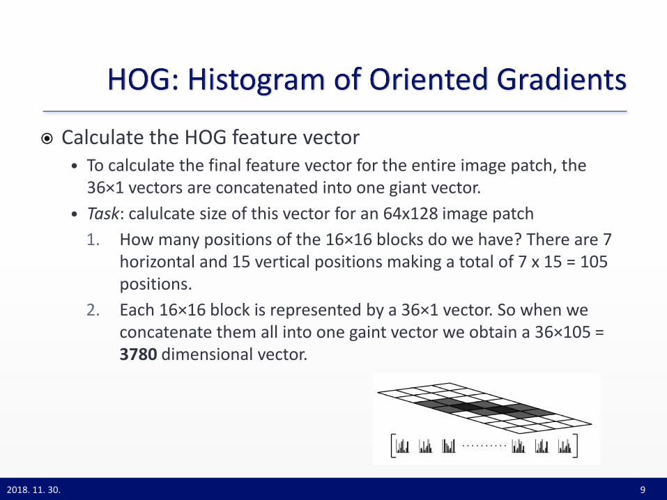
Calculate the HOG feature vector• To calculate the final feature vector for the entire image patch, the

36×1 vectors are concatenated into one giant vector.

• Task: calulcate size of this vector for an 64x128 image patch

1. How many positions of the 16×16 blocks do we have? There are 7 horizontal and 15 vertical positions making a total of 7 x 15 = 105 positions.

2. Each 16×16 block is represented by a 36×1 vector. So when we concatenate them all into one gaint vector we obtain a 36×105 = 3780 dimensional vector.

2018. 11. 30. 9

Plotting the 9×1 normalized histograms in the 8×8 cells.

• dominant direction of the histogram captures the shape of the person, especially around the torso and legs.

2018. 11. 30. 10

V. Classification• Linear SVM

• For pedestrian detection it was trained on 64x128 sized samples (positive and negative images).

HOG inspired methods• A fast version of HOG with..

variable block size,

AdaBoost for feature selection,

cascade of rejectors and integral image representation.

70x faster than the original

• Motion Flow based HOG

2018. 11. 30. 11

Zhu, Q., Yeh, M., Cheng, K., and Avidan, S., „Fast Human Detection Using a Cascade of Histograms of Oriented Gradients”. In Proceedings of the2006 IEEE Computer Society, CVPR, Washington, DC, 1491-1498.N. Dalal, B. Triggs, C. Schmid, „Human Detection Using Oriented Histograms of Flow and Appearance”, In Proceedings of the European Conferenceon Computer Vision, Graz, Austria, May 2006.

Computationally effective texture descriptor.• Comparable to the state of the art,

• while computable in O(n) time.

• Robust to monotonic changes in the illumination, no image preprocessing or parameter tuning is required.

• Produces a compact, 59 bin descriptor (SIFT has 128 bins), so it is faster to match.

• Proved it’s efficiency in many applications:

Face detection, recognition, facial expression analysis

Image retrieval, biometrics

Texture analysis, image segmentation

…

2018. 11. 30. 12

Ojala T, Pietikäinen M & Mäenpää T (2002) Multiresolution gray-scale and rotation invariant texture classification with Local Binary Patterns. IEEE Transactions on Pattern Analysis and Machine Intelligence 24(7):971-987.

Main steps of the algorithm:• Calculate the difference of a pixel and its neighbors in a fixed radius

circular pattern:

• Invariant to local contrast magnitude and global illumination changes.

• Represent the result as a decimal number:

2018. 11. 30. 13

Marc Norvig’s talk: Introduction to Local Binary Patternshttp://files.meetup.com/4379272/BIPCVG_LocalBinaryPatterns_2013.01.16.pdf

Binarize the result

10001011 139

Binary number Decimal number

Notes on implementation: • the circular pattern does not fit very well on the

squared sampling grid.

• On grid points use sample data directly

• Off grid points use interpolation

2018. 11. 30. 14


Main steps of the algorithm (continued):• Calculate the LBP for each point of the patch.

• Build the histogram of the LBP values.

• This histogram is the descriptor of the patch.

• To match histograms the following measures is commonly used:

Histogram Intersection

Chi-Squared

Log-Likelihood

2018. 11. 30. 15


Uniform LBP:• So far we have 256 dimension descriptor (256 bin histogram of 256

possible different desciptor values), promised fewer than 64D!

• In general 90% of the LBPs has at most two contiguous regions in it:

There are 2 patterns with one region

There are 7 patterns with 2 regions

• For each of the 7 pattern with 2 regions there can be 8 different orientations.

• We keep one joker bin for everything else: 2+7*8+1 = 59 bin descriptor

• We reduced the #dimensions from 256 to 59 and as a bonus the resulted descriptor is more robust to noise.

2018. 11. 30. 16


58 Uniform Local Binary Patterns plus one

2018. 11. 30. 17

Robustness against monotonic changes of illumination

2018. 11. 30. 18


Application of LBP for…• Face recognition:

• Image segmentation:

2018. 11. 30. 19


SIFT, SURF and HOG:• are based on histograms of gradients, which is costly to compute,

• the size of the descriptors can be problematic if we have many of them

• also SIFT is patent protected.

Binary descriptors use simple intensity value comparisons tocreate binary strings to encode the information of the patch:

Fast to compute,

Easy to store

Fast to match (Hamming distance == XOR)

Binary Descriptors:• BRIEF, ORB

• FREAK

• BRISK

2018. 11. 30. 20

Gil's Computer vision blog: http://gilscvblog.wordpress.com/2013/08/26/tutorial-on-binary-descriptors-part-1/

In general, Binary descriptors are composed of three parts: • sampling pattern,

• orientation compensation and

• sampling pairs.

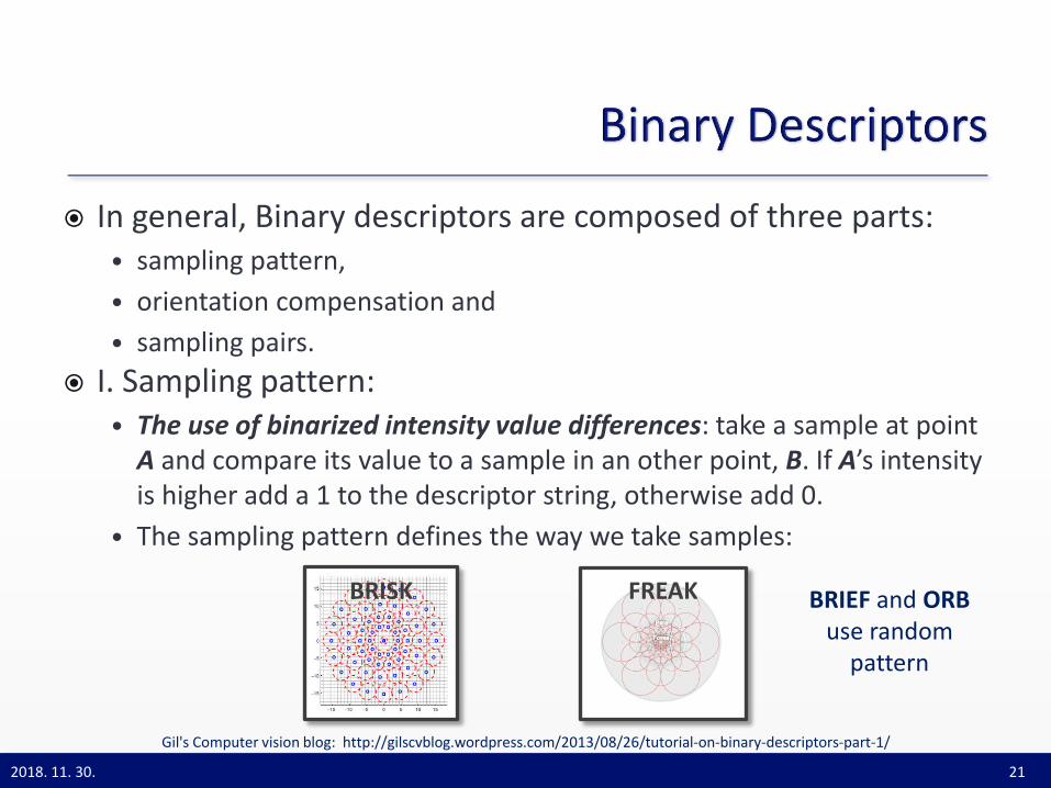
I. Sampling pattern:• The use of binarized intensity value differences: take a sample at point

A and compare its value to a sample in an other point, B. If A’s intensity is higher add a 1 to the descriptor string, otherwise add 0.

• The sampling pattern defines the way we take samples:

2018. 11. 30. 21


BRISK FREAK BRIEF and ORBuse random

pattern

Sampling pairs:• BRIEF uses random sampling pattern and selects random pairs from

them.

• BRISK uses only short distance pairs from the predefined pattern

2018. 11. 30. 22


BRISK

• FREAK and ORB learns the sampling pairs so that

their information content is maximal, the redundancy is minimal between the pairs,

and the variance of the pairs is high to make the feature more discriminative.

• In case of FREAK the resulted pairs follow a coarse-to-fine structure:

The first pairs selected are comparing points in the outer ring

The last selected points make comparisons in the dense region

This resembles to the way the human vision operates.

2018. 11. 30. 23

FREAK


II. Orientation Compensation:• The binary pairs are sensitive to rotation.

• In the orientation compensation phase the orientation angle of thepatch is measured and the pairs are rotated by that angle to ensurethat the description is rotation invariant.

• Different descriptors have different methods for orientationcompensation:

BRIEF: does not have orientation compensation

ORB: based on the moments of the patch

BRISK: comparing gradient of long pairs

FREAK: comparing gradient of preselected pairs

2018. 11. 30. 24


III. Matching:1. Given two keypoint, first procedure the binary descriptor for both of

them, using the same sampling pattern and the same sequence ofpairs.

2. Once we have two binary string, just count the number of bits wherethe strings are different.

• FREAK uses a cascade approach (based on its special coarse to fineorganization of sampling pairs):

It starts with matching only the first 128 bits, which can eliminate90% of the candidates can be rejected (in average).

If the difference for the first 128 bits is lower than a threshold itchecks the next 128 bits.

2018. 11. 30. 25


Performance:• Which one is the best depends on the task:

BRIEF outperforms BRISK, ORB and FREAK in photometric changes –blur, illumination changes and JPEG compression.

When there are view-point changes, FREAK slightly outperforms ORB and BRISK, but performs worse than BRIEF.

When there are zoom + rotation changes, FREAK slightly outperforms BRIEF and BRISK, but performs worse than ORB.

2018. 11. 30. 26

Gil's Computer vision blog: http://gilscvblog.wordpress.com/2013/11/08/a-tutorial-on-binary-descriptors-part-4-the-brisk-descriptor/

BRISK

2018. 11. 30. 27

M. Calonder, V. Lepetit, M. Ozuysal, T. Trzcinski, C. Strecha, and P. Fua, ”Computing a Local Binary Descriptor Very Fast,” IEEE Transactions on Pattern Analysis and Machine Intelligence 2012

BRIEF (Binary Robust Independent Elementary Features)

Introduction to descriptors: http://gilscvblog.wordpress.com/2013/08/18/a-short-introduction-to-descriptors/

C. Harris and M. Stephens (1988). "A combined corner and edge detector". "Proceedings of the 4th Alvey Vision Conference". pp. 147–151.

Lowe, „Object recognition from local scale-invariant features”, In: The Proceedings of the Seventh IEEE International Conference on, Vol. 2 (1999), pp. 1150-1157 vol.2.

Y. Ke and R. Sukthankar, “PCA-SIFT: A More Distinctive Representation for Local Image Descriptors,” Proc. Conf. Computer Vision and Pattern Recognition, pp. 511-517, 2004.

H. Bay, T. Tuytelaars, L. Van Gool "SURF: Speeded Up Robust Features", Proceedings of the 9th European Conference on Computer Vision, Springer LNCS volume 3951, part 1, pp 404--417, 2006.

N. Dalal,B. Triggs, „Histograms of Oriented Gradients for Human Detection” In Proceedings of IEEE Conference Computer Vision and Pattern Recognition, San Diego, USA, pages 886-893, June 2005.

Zhu, Q., Yeh, M., Cheng, K., and Avidan, S., „Fast Human Detection Using a Cascade of Histograms of Oriented Gradients”. In Proceedings of the 2006 IEEE Computer Society, CVPR, Washington, DC, 1491-1498.

N. Dalal, B. Triggs, C. Schmid, „Human Detection Using Oriented Histograms of Flow and Appearance”, In Proceedings of the European Conference on Computer Vision, Graz, Austria, May 2006.

2018. 11. 30. 28

http://gilscvblog.wordpress.com/2013/08/18/a-short-introduction-to-descriptors/


Michael Calonder, Vincent Lepetit, Christoph Strecha, and Pascal Fua, “BRIEF: Binary Robust Independent Elementary Features”, 11th European Conference on Computer Vision (ECCV), Heraklion, Crete. LNCS Springer, September 2010.

Alahi, Alexandre, Raphael Ortiz, and Pierre Vandergheynst. “Freak: Fast retina keypoint.” Computer Vision and Pattern Recognition (CVPR), 2012 IEEE Conference on. IEEE, 2012.

Leutenegger, Stefan, Margarita Chli, and Roland Y. Siegwart. “BRISK: Binary robust invariant scalable keypoints.” Computer Vision (ICCV), 2011 IEEE International Conference on. IEEE, 2011.

Rublee, Ethan, et al. “ORB: an efficient alternative to SIFT or SURF.” Computer Vision (ICCV), 2011 IEEE International Conference on. IEEE, 2011.

Ojala T, Pietikäinen M & Mäenpää T (2002) Multiresolution gray-scale and rotation invariant texture classification with Local Binary Patterns. IEEE Transactions on Pattern Analysis and Machine Intelligence 24(7):971-987.

Marc Norvig’s talk: Introduction to Local Binary Pattern: http://files.meetup.com/4379272/BIPCVG_LocalBinaryPatterns_2013.01.16.pdf

2018. 11. 30. 29

http://files.meetup.com/4379272/BIPCVG_LocalBinaryPatterns_2013.01.16.pdf

ppke-itk lecture 11.gradient computation 2. orientation binning 3. block description 4. block...

Documents