practical approximate analysis of beams and frames_ lecture notes in mechanics 1-nabil...
DESCRIPTION
Aproximacion practica vigasTRANSCRIPT


Lecture Notes in Mechanics 1
PracticalApproximateAnalysis of Beamsand Frames
Nabil Fares, Ph.D.

Library of Congress Cataloging-in-Publication Data on file.
Published by American Society of Civil Engineers1801 Alexander Bell DriveReston, Virginia 20191www.asce.org/pubs
Any statements expressed in these materials are those of the individual authors and donot necessarily represent the views of ASCE, which takes no responsibility for anystatement made herein. No reference made in this publication to any specific method,product, process, or service constitutes or implies an endorsement, recommendation, orwarranty thereof by ASCE. The materials are for general information only and do notrepresent a standard of ASCE, nor are they intended as a reference in purchasespecifications, contracts, regulations, statutes, or any other legal document.
ASCE makes no representation or warranty of any kind, whether express or implied,concerning the accuracy, completeness, suitability, or utility of any information,apparatus, product, or process discussed in this publication, and assumes no liabilitytherefor. This information should not be used without first securing competent advicewith respect to its suitability for any general or specific application. Anyone utilizing thisinformation assumes all liability arising from such use, including but not limited toinfringement of any patent or patents.
ASCE and American Society of Civil Engineers—Registered in U.S. Patent andTrademark Office.
Photocopies and permissions. Permission to photocopy or reproduce material from ASCEpublications can be obtained by sending an e-mail to [email protected] or by locatinga title in ASCEs online database (http://cedb.asce.org) and using the “Permission toReuse” link. Bulk reprints. Information regarding reprints of 100 or more copies isavailable at http://www.asce.org/reprints.
Copyright c© 2012 by the American Society of Civil Engineers.All Rights Reserved.
ISBN 978-0-7844-1222-0 (paper)ISBN 978-0-7844-7685-7 (e-book)
Manufactured in the United States of America.
18 17 16 15 14 13 12 1 2 3 4 5

Lecture Notes in MechanicsAristotle and Archytas defined mechanics as the “organization of thoughttowards solving perplexing problems that are useful to humanity.” In the spiritAristotle and Archytas, Lecture Notes in Mechanics (LNMech) tran-scends the traditional division of mechanics and provides a forum forpresenting state-of-the-art research that tackles the range of complex is-sues facing society today.
LNMech provides for the rapid dissemination of comprehensivetreatments of current developments in mechanics, serving as a repositoryand reference for innovation in mechanics, across all relevant applicationdomains.
LNMech publishes original contributions, including monographs,extended surveys, and collected papers from workshops and confer-ences. All LNMech volumes are peer reviewed, available in print andonline through ASCE, and indexed by the major scientific indexing andabstracting services.
Series EditorRoger Ghanem
Editorial BoardYounane Abousleiman, Ph.D., University of OklahomaRoberto Ballarini, Ph.D., P.E., University of MinnesotaRonaldo I. Borja, Ph.D., Stanford UniversityShiyi Chen, Ph.D., Peking UniversityTerry Friesz, Ph.D., Pennsylvania State UniversityBojan B. Guzina, Ph.D., University of MinnesotaIoannis Kevrekidis, Ph.D., Princeton UniversityMohammad A. Khaleel, P.E., Ph.D., Pacific Northwest National
LaboratoryPeter Kuhn, Ph.D., University of California at San DiegoArif Masud, Ph.D., University of Illinois, Urbana-ChampaignIgor Mezic, Ph.D., University of California at Santa BarbaraKaram Sab, Ph.D., Ecole Normale des Ponts et ChausseesAndrew W. Smyth, Ph.D., Columbia UniversityChristian Soize, Ph.D., Universite Paris-EstPol D. Spanos Ph.D., P.E., Rice UniversityLizhi Sun, Ph.D., University of California at IrvineZhigang Suo, Ph.D., Harvard UniversityPaul Torrens, Ph.D., University of MaryandFranz-Josef Ulm, Ph.D., P.E., Massachusetts Institute of Technology
LNMech 1 Practical Approximate Analysis of Beams and FramesNabil Fares, Ph.D.
LNMech 2 Stochastic Models of Uncertainties in ComputationalMechanicsChristian Soize, Ph.D.
Contents
Preface vii
1 Approximate Analysis of Beams and Frames withno Sidesway 11.1 Introduction to Sketching . . . . . . . . . . . . . . . . . . . . . . . . . . . . . 11.2 Passive Members in Continuous Beams and Frames . . . . . . . . . . . 41.3 Beam with a Moment Applied at One End and Resisting
at the Other . . . . . . . . . . . . . . . . . . . . . . . . . . . . . . . . . . . . . 111.4 Example: Continuous Beam with Moment Applied
at Only One Node . . . . . . . . . . . . . . . . . . . . . . . . . . . . . . . . . 161.5 Outline of Approximate Method for Analyzing Structures
with No Sidesway . . . . . . . . . . . . . . . . . . . . . . . . . . . . . . . . . . 201.6 Beam with a Uniform Load . . . . . . . . . . . . . . . . . . . . . . . . . . . . 221.7 Example: Uniform Load . . . . . . . . . . . . . . . . . . . . . . . . . . . . . . 391.8 Beam with a Point Force . . . . . . . . . . . . . . . . . . . . . . . . . . . . . 421.9 Example: Point Force . . . . . . . . . . . . . . . . . . . . . . . . . . . . . . . 671.10 Comments and Examples on Multiple Loads . . . . . . . . . . . . . . . . . 711.11 Beam with Two or More Internal Hinges . . . . . . . . . . . . . . . . . . . . 791.12 Beam with One Internal Hinge, a Moment Applied at One End
and Resisting at the Other . . . . . . . . . . . . . . . . . . . . . . . . . . . . 871.13 Beam with One Internal Hinge and a Uniform Load . . . . . . . . . . . . . 941.14 Beam with One Internal Hinge and a Point Force . . . . . . . . . . . . . . 98
2 Approximate Analysis of Frames with Sidesway 1052.1 The Cantilever and the Single Floor Portal Frame . . . . . . . . . . . . . . 1052.2 Approximate Analysis of Single Floor Frames Subject
to a Horizontal Load . . . . . . . . . . . . . . . . . . . . . . . . . . . . . . . . 1152.3 Sketching Single Floor Portal Frames . . . . . . . . . . . . . . . . . . . . . 1242.4 The Column with Rotary Springs and Moments at Both Ends . . . . . . 1312.5 Approximate Analysis of Multiple Floor Frames Subject
to Horizontal Loads . . . . . . . . . . . . . . . . . . . . . . . . . . . . . . . . 1412.6 A Note on the Lumped Mass Model for Buildings . . . . . . . . . . . . . . 1522.7 Sketching Multiple Floor Frames Subject to Horizontal Loads . . . . . . 1602.8 Notes on Sidesway Due to Vertical Loads or Applied Couples . . . . . . 171
v

vi Practical Approximate Analysis of Beams and Frames
3 Estimating Displacements in Beams and Frames 1853.1 Maximum Vertical Displacements in Beams . . . . . . . . . . . . . . . . . 1853.2 Estimating Moment of Inertia . . . . . . . . . . . . . . . . . . . . . . . . . . 1913.3 Relative Vertical Displacements versus Strain in Beams . . . . . . . . . . 2033.4 Side Displacements of Frames Subject to Side Loads . . . . . . . . . . . 2113.5 Obtaining Rotary Stiffness Factors from Slope Measurements
in Beams . . . . . . . . . . . . . . . . . . . . . . . . . . . . . . . . . . . . . . . 225
4 Approximate Influence Lines for IndeterminateBeams 2354.1 Introduction to Influence Lines . . . . . . . . . . . . . . . . . . . . . . . . . . 2354.2 Exact Influence Lines for Statically Determinate Beams . . . . . . . . . . 2424.3 Approximate Influence Lines for Statically
Indeterminate Structures . . . . . . . . . . . . . . . . . . . . . . . . . . . . . 270
Appendixes
A Beams—End-Moments and Inflection Points 317A.1 Moment End-Loaded Beam . . . . . . . . . . . . . . . . . . . . . . . . . . . 317A.2 Uniformly Distributed Load . . . . . . . . . . . . . . . . . . . . . . . . . . . . 319A.3 Point Force . . . . . . . . . . . . . . . . . . . . . . . . . . . . . . . . . . . . . . 321
B Column—Shear Stiffness, End-Moments andInflection Points 327B.1 Cantilever . . . . . . . . . . . . . . . . . . . . . . . . . . . . . . . . . . . . . . 327B.2 Column for Single Story Building . . . . . . . . . . . . . . . . . . . . . . . . 328B.3 Column for Multi-Story Building—First Floor . . . . . . . . . . . . . . . . . 330B.4 Column for Multi-Story Building—Top Floor (Top and Bottom
Beams Similar) . . . . . . . . . . . . . . . . . . . . . . . . . . . . . . . . . . . 332B.5 Column for Multi-Story Building—General Case . . . . . . . . . . . . . . . 333
C Beams—Deflections and Rotations 335C.1 Displacements at Any Location . . . . . . . . . . . . . . . . . . . . . . . . . 335C.2 Rotations at Any Location . . . . . . . . . . . . . . . . . . . . . . . . . . . . 338C.3 Uniform Load—Mid Displacements . . . . . . . . . . . . . . . . . . . . . . . 340C.4 Point Force—Centrally Loaded—Mid Displacements . . . . . . . . . . . . 342C.5 Point force—Loaded Anywhere—Mid Displacements . . . . . . . . . . . 344C.6 Point Moment—Loaded Anywhere—Mid Displacements . . . . . . . . . 347C.7 Cantilever—Various Special Cases—Displacements . . . . . . . . . . . . 350

Practical Approximate Analysis of Beams and Frames vii
D Useful Results for Influence Lines 353D.1 Influence Lines for Vertical Force Reactions . . . . . . . . . . . . . . . . . 353D.2 Influence Lines for Shear Forces . . . . . . . . . . . . . . . . . . . . . . . . 355D.3 Influence Lines for Bending Moments . . . . . . . . . . . . . . . . . . . . . 355D.4 Transition Member . . . . . . . . . . . . . . . . . . . . . . . . . . . . . . . . . 357
Index 359

This page intentionally left blank

Preface
The aim of this book is to present a new approach to approximately an-alyze beams and frames. The new approach has the following desirablefeatures:
• The approach is relatively short and simple, robust with good accu-racy and is practically applicable to realistic problems. Some formerstudents who have learned these methods have reported that, in theworkplace, they have been able to complete an accurate approximateanalysis of a structure in the time it took their colleagues to enter adescription of the structure into a computer model.
• The approach is naturally amenable to parametric studies and resultspresenting summaries and ranges of behavior covering a wide rangeof situations are pervasive throughout the book. This builds a knowl-edge base that a practitioner can use to anticipate the range of possibleresults that may be encountered with a new structure.
• The approach has strong visual components, especially in the empha-sis on consistent semi-quantitative sketching of deformed structures.These sketches are especially useful as repositories and enhancementsto experience. The reason is that: i) There is a synergy between suchsketches and moment diagrams which are essential for design so thatexperience in one translates into improvements in the other. ii) Bothdeeper insight and more experience with the analysis of beam andframe structures allows the user to be more accurate or to add moredetails in the sketches of the deformed shapes. Having drawn suchimproved sketches, the user then remembers and consolidates bothinsight and experience. iii) Comparisons between the sketches of thedeformed structures and moment diagrams allows inconsistencies tobe detected and hence, reduces potential manual errors.
• The approach generally localizes all dimensional quantities in one ora few factors so that the main parameters to be estimated are the rel-evant relative stiffnesses. This non-dimensionalization also generallyleads to having all calculated non-dimensional quantities lying be-tween negative and positive one. Both of these effects reduce the like-lihood of manual error because the range of possible values become
ix

x Practical Approximate Analysis of Beams and Frames
rather limited and because one of the main sources of error is usuallyin dimensional calculations and unit conversions. Extensive experi-ence and practice with the method and with typical relative stiffnessesalso eventually leads to results being recalled, due to the limited rangeof common non-dimensional results, rather than calculated which fur-ther enhances the speed and accuracy of the user.
• In addition to moment diagrams, the approach also addresses how toestimate deflections, influence lines and moments of inertia.
• The approach identifies a possible framework for the non-destructiveevaluation of framed structures. A specific experimental methodbased on that framework is proposed and analyzed.
• The approach sheds light on the limits of applicability of the widelyused lumped-mass model for the dynamical analysis of structures. Theimplications are presented and discussed.
For all the above reasons, we recommend this book to both studentsand practitioners. However, we note that the proposed new approximateapproach must be complemented with other material in order to consti-tute a good second course in structural analysis. For example, a goodsecond course would include the approximate approach in this book,the direct stiffness method, training on the use of some structural analy-sis software and, if time permits, exposure to one or two other advancedstructural analysis topics.
Finally, the main objective of this book is to provide students andpractitioners of structural mechanics with a new analysis approach thatcomplements the use of software but provides a critical role for the struc-tural engineer. That role is necessarily at a higher conceptual level andmust cater to the strengths of humans which is the recognition of pat-terns, preferably visible ones. The author hopes that this work would en-courage others to refine and extend this approach or its essence to otherareas of structural engineering and indeed to most other topics wheresoftware is displacing much of the skills that were previously providedby people.

Dedication
This book is dedicated to Professor Jim Rice who taught me to ’figurethe answer and then do the calculation’ and to my wife Maha who sup-ported and encouraged me to complete this book.

This page intentionally left blank
Chapter 1
Approximate Analysisof Beams and Frameswith No Sidesway
1.1 Introduction to SketchingThroughout this book, we will be concerned with sketching the deforma-tions of beams and frames. Such sketches, when qualitatively precise, il-lustrate the behavior of structures in a visually rich and informative way.For example, such sketches may be directly related to bending momentdiagrams which are a basis for design. By qualitatively precise sketches,we mean that we will be mostly concerned with: i) getting the right signof the curvature at each point which implies ii) approximately identify-ing the location of each inflection point which are locations of zero curva-ture and hence zero moment, iii) getting the right sign of the slopes at theends of members and iv) getting the right sign of the displacements. Ingeneral, we will greatly exaggerate the magnitude of the displacementsand place minor emphasis on the details of the deformed shape beyondthe above concerns.
To start our sketching program, we will observe the deformation ofa real but very slender beam. Specifically, we will consider the defor-mations of a long slender straw shown in figures 1.1a–d. As long as thematerial is linear elastic, the shape of that slender straw will be represen-tative of any beam under similar loading conditions but the straw willhave relatively very large deformations. While sketching the deforma-tion of a beam, we will talk of displacement, slope and curvature. Fora horizontal beam, positive displacement will be up, positive slope willcorrespond to a counter-clockwise rotation from the horizontal and theconvention for positive and negative curvature is shown in figure 1.2.
1

2 Practical Approximate Analysis of Beams and Frames
(a) applied moment—fixed (b) applied moment—pinned
(c) applied moment—spring (d) applied moment—fixed then sheared
Figure 1.1. Loading of a simple slender beam.
positive curvature negative curvature
Figure 1.2. Convention for positive and negative curvatures.
Let’s start by sketching figure 1.1a in a way that is consistent withour objectives. First we draw small straight line “stubs” at each end ofthe beam as shown in figure 1.3a. At the left end, we draw a stub witha positive slope and zero displacement while at the right end we drawa stub with zero slope and zero displacement. Next, we notice that thecurvature near the left end is negative while the curvature at the rightis positive with the inflection point (ie. zero curvature) somewhat closerto the right end. Based on calculations for the case shown in figure 1.1a,the inflection point is calculated to be at one third the length from theright end. Therefore, starting with the left stub, we draw a curve withnegative curvature and, starting with the right stub, we draw a curve
Practical Approximate Analysis of Beams and Frames 3
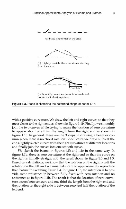
(a) Place slope stubs at the ends
(b) Lightly sketch the curvatures startingfrom the ends
0.33 L
(c) Smoothly join the curves from each endnoting the inflection points
Figure 1.3. Steps in sketching the deformed shape of beam 1.1a.
with a positive curvature. We draw the left and right curves so that theymeet closer to the right end as shown in figure 1.1b. Finally, we smoothlyjoin the two curves while trying to make the location of zero curvatureto appear about one third the length from the right end as shown infigure 1.1c. In general, these are the 3 steps in drawing a beam or col-umn when there is no chord rotation. Specifically, we draw stubs at theends, lightly sketch curves with the right curvatures at different locationsand finally join the curves into one smooth curve.
We sketch the beams in figures 1.1b and 1.1c in the same way. Infigure 1.1b, there is zero curvature at the right end so that the curve onthe right is initially straight with the result shown in figure 1.4 and 1.5.Based on calculations, we know that the rotation on the right is half therotation on the left and we must take care to approximately reproducethat feature in sketching figure 1.4. In figure 1.1c, the intention is to pro-vide some resistance in-between fully fixed with zero rotation and noresistance as in figure 1.1b. The result is that the location of zero curva-ture occurs between zero and one third the length from the right end andthe rotation on the right side is between zero and half the rotation of theleft end.

4 Practical Approximate Analysis of Beams and Frames
(a) Place slope stubs at the ends
(b) Lightly sketch the curvaturesstarting from the ends
(c) Smoothly join the curves fromeach end noting the inflectionpoints
Figure 1.4. Sketching the deformedshape of beam 1.1b.
(a) Place slope stubs at the ends
(b) Lightly sketch the curvaturesstarting from the ends
(c) Smoothly join the curves fromeach end noting the inflectionpoints
Figure 1.5. Sketching the deformedshape of beam 1.1c.
1.2 Passive Members in ContinuousBeams and Frames
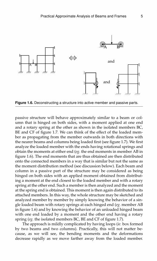
How does sketching the deformation and bending moment of singlemembers help us in doing the same for assemblies of such members suchas beams and frames? To explain, we will first define a passive part of astructure to be that part, if any, that has no loads applied and that has nosidesway in any of its members. Neglecting axial deformations, a loadedbeam or column connected to a passive part of a structure at a node willexperience the equivalent of a linear rotary spring at that node as illus-trated in figure 1.6. In that figure, we see the effect of the passive struc-tures on member AB being reduced to two rotary springs at the ends.The behavior of the loaded member can then be sketched and analyzedby knowing the behavior of a single loaded member (beam or column)with hinges and rotary springs at each end.
After considering the behavior of the loaded member, we considerthe members in the passive structures (eg. the members to the left andright of member AB in figure 1.6). We observe that every member of a
Practical Approximate Analysis of Beams and Frames 5
A B
⇔A B
and
and
Figure 1.6. Deconstructing a structure into active member and passive parts.
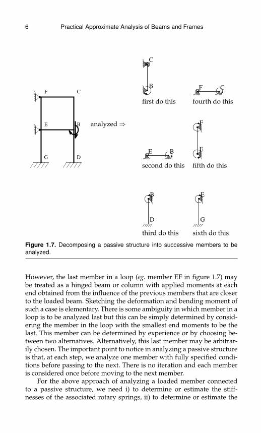
passive structure will behave approximately similar to a beam or col-umn that is hinged on both sides, with a moment applied at one endand a rotary spring at the other as shown in the isolated members BC,BE and CF of figure 1.7. We can think of the effect of the loaded mem-ber as propagating from the member outwards in both directions withthe nearer beams and columns being loaded first (see figure 1.7). We firstanalyze the loaded member with the ends having rotational springs andobtain the moments at either end (eg. the end moments in member AB infigure 1.6). The end moments that are thus obtained are then distributedonto the connected members in a way that is similar but not the same asthe moment distribution method (see discussion below). Each beam andcolumn in a passive part of the structure may be considered as beinghinged on both sides with an applied moment obtained from distribut-ing a moment at the end closest to the loaded member and with a rotaryspring at the other end. Such a member is then analyzed and the momentat the spring end is obtained. This moment is then again distributed to itsattached members. In this way, the whole structure may be sketched andanalyzed member by member by simply knowing the behavior of a sin-gle loaded beam with rotary springs at each hinged end (eg. member ABin figure 1.6) and by knowing the behavior of an unloaded hinged beamwith one end loaded by a moment and the other end having a rotaryspring (eg. the isolated members BC, BE and CF of figure 1.7).
The approach is mildly complicated by having loops (ie. box formedby two beams and two columns). Practically, this will not matter be-cause, as we will see, the bending moments and the deformationsdecrease rapidly as we move farther away from the loaded member.
6 Practical Approximate Analysis of Beams and Frames
G D
E B
F C
analyzed⇒
B
C
first do this
CF
fourth do this
BE
second do this
F
E
fifth do this
B
D
third do this
E
G
sixth do this
Figure 1.7. Decomposing a passive structure into successive members to beanalyzed.
However, the last member in a loop (eg. member EF in figure 1.7) maybe treated as a hinged beam or column with applied moments at eachend obtained from the influence of the previous members that are closerto the loaded beam. Sketching the deformation and bending moment ofsuch a case is elementary. There is some ambiguity in which member in aloop is to be analyzed last but this can be simply determined by consid-ering the member in the loop with the smallest end moments to be thelast. This member can be determined by experience or by choosing be-tween two alternatives. Alternatively, this last member may be arbitrar-ily chosen. The important point to notice in analyzing a passive structureis that, at each step, we analyze one member with fully specified condi-tions before passing to the next. There is no iteration and each memberis considered once before moving to the next member.
For the above approach of analyzing a loaded member connectedto a passive structure, we need i) to determine or estimate the stiff-nesses of the associated rotary springs, ii) to determine or estimate the
Practical Approximate Analysis of Beams and Frames 7
end moments at the ends of loaded members attached to passive struc-tures and iii) to quantitatively analyze a hinged member with an appliedmoment at one end and a rotary spring at the other (see for examplefigures 1.10). This will allow us to completely specify then analyze eachmember of a passive structure. In the next section, we will address thethird point which is the analysis of the member shown in figure 1.11. Inthe sections after that we will also address how to analyze various typesof loaded beams with rotational springs at each end. In this section, wewill address the question of how to handle the first point which is theestimation of the stiffness of rotary springs representing the behavior ofpassive structures.
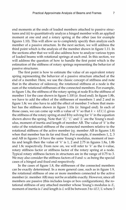
The first point is how to estimate the value of an equivalent rotaryspring representing the behavior of a passive structure attached at theend of a member. Here, we use the classic concept of stiffness and notethat in the absence of sidesway, the rotational stiffness at a node is thesum of the rotational stiffnesses of the connected members. For example,in figure 1.8a, the stiffness of the rotary spring at node B is the stiffness ofmember 1 for the case shown in figure 1.10f (ie. fixed end). In figure 1.8b,we have to add the effect of the stiffnesses of members 1 and 2 and infigure 1.8c we also have to add the effect of member 3 where that mem-ber has the stiffness shown in figure 1.10a (ie. hinged end). In each ofthose cases, we can come up with a value of ‘k’ so that k × 4EI/L givesthe stiffness of the rotary spring at end B by solving for ‘k’ in the equationshown above the spring. Note that ‘E,’ ‘I,’ and ‘L’ are the Young’s mod-ulus, moment of inertia and length of member AB. The value of ‘k’ is theratio of the rotational stiffness of the connected members relative to therotational stiffness of the active member (eg. member AB in figures 1.8)when that member has its far end fixed. For example, if members 1, 2, 3and AB in figures 1.8 have the same Young’s modulus, moment of iner-tia and length then the value of ‘k’ is 1, 2 and 2.75 in figures 1.8a, 1.8band 1.8c respectively. From now on, we will refer to ‘k’ as the k-value,rotary stiffness factor or stiffness factor of the rotary spring at a node.Typical rotary stiffness factors in structures are in the range of 0.75 to 3.We may also consider the stiffness factors of 0 and∞ as being the specialcases of a hinged and fixed end respectively.
In the cases of figure 1.8, the stiffnesses of the connected memberscan be exactly determined. In a more general case, such as in figure 1.9,the rotational stiffness of one or more members connected to the activemember (ie. member AB) may not be available exactly. However, since allmembers are passive (this includes loops or box configurations), the ro-tational stiffness of any attached member whose Young’s modulus is E,moment of inertia is I and length isLwill be between 3 to 4EI/Lwhere 3

8 Practical Approximate Analysis of Beams and Frames
AB
EI
L
EI1
L1
Mapplied
⇔ AB
Mapplied4
EI1
L1
= k ´ 4
EI
L
(a)
A B
EI1
L1
EI2L2
Mapplied
⇔ A B
Mapplied4
EI1
L1
+4
EI2
L2
= k ´ 4
EI
L
(b)
A B
EI1
L1
EI2L2
EI3L3Mapplied
⇔ A B
Mapplied4
EI1
L1
+4
EI2
L2
+3
EI3
L3
= k ´ 4
EI
L
(c)
Figure 1.8. Determining the exact stiffness in special cases.
A B
EI1
L1
EI4
L4
EI2L2
Mapplied
⇔A B
EI1
L1
EI2L2
Mapplied
⇔
AB
MappliedH3 to 4L
EI1
L1
+ 4
EI2
L2
= k ´ 4
EI
L ≈ AB
Mapplied
4
EI1
L1
+ 4
EI2
L2
= k ´ 4
EI
L
Figure 1.9. Estimating the rotational stiffness at node B for member AB.

Practical Approximate Analysis of Beams and Frames 9
0M�Θ = 0.75´4
EI
L
(a)
0.75´4EI
L
M�Θ = 0.86´4EI
L
(b)
1.00´4EI
L
M�Θ = 0.88´4EI
L
(c)
1.50´4EI
L
M�Θ = 0.90´4EI
L
(d)
2.00´4EI
L
M�Θ = 0.92´4EI
L
(e)
¥M�Θ = 1.00´4
EI
L
(f)
Figure 1.10. Effective bending stiffness at one end of a beam when a spring isat the other end.
is for a hinged end and 4 is a for a fixed end as shown in figures 1.10a–f.At this point, we could determine the exact rotational stiffness of a mem-ber attached to a rotational spring as shown for some selected cases infigures 1.10, but instead, we can get a good estimate by simply usinga value of 4EI/L for any such member. This will, of course, usuallyoverestimate the stiffness contribution of that member. This procedureis illustrated in figure 1.9 where the contribution of member 1 to the ro-tational stiffness at B is estimated as 4(EI1/L1). In the next section, theanalysis will indicate that such an estimate leads to a maximum errorof less than 4% for the transmitted moment relative to the applied mo-ment at the other end (eg. error in moment at B relative to moment at Aof member AB in figure 1.9) and less than 2.5% for the distance of theinflection point from the rotational spring relative to the length of thebeam (eg. the distance of the inflection point from node B in member ABrelative to the total length of AB of figure 1.9). Experience with usingsuch an estimate along with other associated approximations indicatesthat the overall analysis of a structure using this method will give resultsthat are within 5 to 10% of the exact results in terms of bending moments

10 Practical Approximate Analysis of Beams and Frames
except for moments that are small compared to the maximum moment inthe structure (ie. moments that are less than about 5% of the maximum).
The second point that was needed to analyze all members in a pas-sive structure is to determine the end moment at the loaded ends of themembers in a passive structure. This is again done using the idea ofstiffness or of relative stiffness as is done in the classic method of mo-ment distribution. The difference is that the active member is removedfrom the joint and its presence is indicated by the moment transmittedfrom the active member to that point. For example, the moment at B onthe passive structure BCDEFG in figure 1.7 will be distributed on mem-bers BC, BE and BD with no contribution of the stiffness of member AB(see figure 1.5). Again, we encounter the problem of not having availablethe exact rotational stiffness of one or more members connected to theactive member. This will again be handled by replacing the rotationalstiffness of a connected member which is between 3 to 4EI/L by 4EI/L.The maximum error on the distributed bending moment that is incurredin such a procedure will be less than 7.2%. This maximum error can bedetermined as follows:
Assume there is a node with several attached members where eachmember has a possibly different rotational stiffness. Consider any mem-ber in that group and call it member 1. We now apply a unit mo-ment on the node. The moment that is distributed to member 1 will be(k1/(k1 + krest) where k1 is the rotational stiffness of member 1 and krestis the combined rotational stiffnesses of the rest of the members. We nowconsider the maximum error incurred if we overestimate the rotationalstiffness of member 1 or of any of the other members by a factor of upto (4/3) (ie. the difference of rotational stiffness between a hinged andfixed far end). The result of such an optimization gives a maximum errorrelative to the applied unit moment of 7.2%. Since member 1 was chosenas any member in the group, this is then the maximum error that may beincurred by any member due to distributing a moment over the atachedmembers. In practice, the error is much smaller than 7.2% because theworst case occurs only when one member has a maximum overestima-tion (ie. from hinged to fixed) while all the other members have no over-estimation in their stiffness (ie. all other members have hinged far-ends).
We note that if we want to obtain better estimates in our analysis,we simply have to use better estimates of the rotational stiffness of con-nected members. If we use the exact rotational stiffnesses we will getexact results, which, with the use of extensive tables or formulas maybe done by propagating the rotational stiffness from the supports backto the loaded member. However, such a process can be quite long anderror prone. The rotational stiffnesses indicated in figures 1.10 illustratesa short table of results while the appendices give more extensive tables
Practical Approximate Analysis of Beams and Frames 11
as well as exact formulas. In practice, using the results of figure 1.10a,1.10c and 1.10f and roughly estimating values in between those cases forany given member gives negligible errors in the bending moments ascompared to exact results for most cases.
In summary, we have described the concept of an active memberconnected to passive parts of a structure. The active member may beanalyzed by considering the member with its applied loads and withrotational springs at its ends. We obtain the moments at the spring endsand then distribute them over the attached members. Subsequently, eachmember in a passive part of the structure may be analyzed by consider-ing a member with one end having a hinge and an applied moment equalto its distributed moment while at the other end having a hinge with arotary spring. The moment at this rotary spring is again distributed to itsattached members to eventually analyze the whole structure.
We have described how to distribute a moment onto the attachedmembers and how to estimate the stiffness of the rotary springs involvedin this process. In the next section, we will study the behavior of a mem-ber with a hinge and an applied moment at one end and a hinge witha rotary spring at the other and in subsequent sections we will describehow to analyze a member with applied loads and with rotational springsat both ends. This will then allow us to analyze any (single) active mem-ber connected to a passive structure and by using the principle of super-position to analyze any beam or frame that has no sidesway.
1.3 Beam with a Moment Applied atOne End and Resisting at the Other
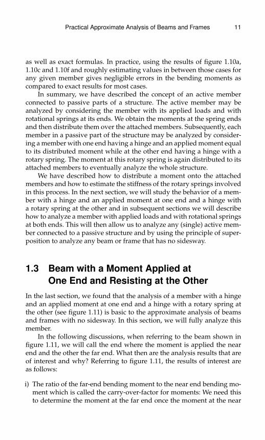
In the last section, we found that the analysis of a member with a hingeand an applied moment at one end and a hinge with a rotary spring atthe other (see figure 1.11) is basic to the approximate analysis of beamsand frames with no sidesway. In this section, we will fully analyze thismember.
In the following discussions, when referring to the beam shown infigure 1.11, we will call the end where the moment is applied the nearend and the other the far end. What then are the analysis results that areof interest and why? Referring to figure 1.11, the results of interest areas follows:
i) The ratio of the far-end bending moment to the near end bending mo-ment which is called the carry-over-factor for moments: We need thisto determine the moment at the far end once the moment at the near

12 Practical Approximate Analysis of Beams and Frames
EI
L
Θnear
Θfar
Mnear k ´ 4EI
L
L - xInflection
x
umax
xat max
Figure 1.11. Beam with moment at near end and rotary spring at far end.
end has been obtained. This result is then essential in obtaining goodquantitative approximations for bending moment diagrams in the pas-sive parts of a structure as described in the previous section.
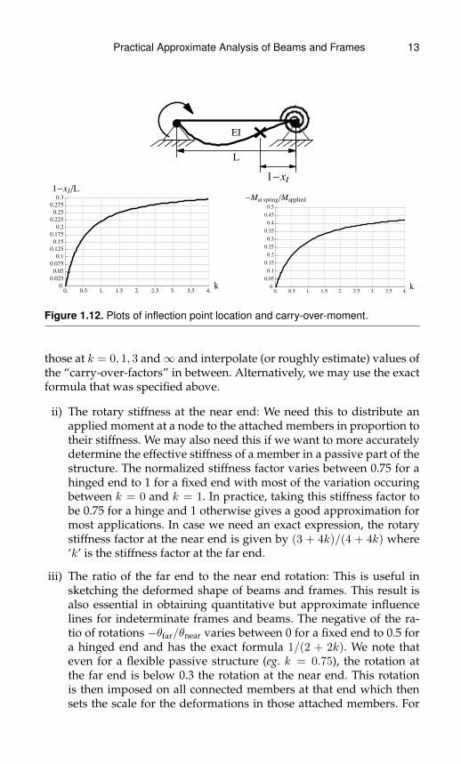
Table 1.1 shows values of−Mfar/Mnear which are always zero or pos-itive because, intuitively, the applied moment is resisted in the oppositesense at the rotary spring. This ratio of moments increases monotoni-cally from 0 (hinged) to 0.5 (fixed) as seen in figure 1.12. In case we needto determine it precisely,−Mfar/Mnear = 2k/(3+4k) where ‘k’ is the stiff-ness factor of the rotary spring. The carry-over factor for moments hasthe value of 0.5 for a fixed end and corresponds to the usual value of thecarry over factor used in moment distribution. From the point of view ofmoment distribution, the approximation method described in the previ-ous section avoids iterations by using more accurate “carry over factors.”In practice, we only need to memorize a few “carry-over-factors” such as
Table 1.1. Hinged Beam with Applied Moment at One End and Rotary Springat Other
k − MfarMnear
Mnearθnear4EI/L
− θfarθnear
1− xinflL
xat maxL
umaxθnearL
0.000 0.000 0.750 0.500 0.000 0.423 0.1920.500 0.200 0.833 0.333 0.167 0.392 0.1760.750 0.250 0.857 0.286 0.200 0.384 0.1721.000 0.286 0.875 0.250 0.222 0.377 0.1681.500 0.333 0.900 0.200 0.250 0.368 0.1642.000 0.364 0.917 0.167 0.267 0.362 0.1613.000 0.400 0.938 0.125 0.286 0.355 0.1584.000 0.421 0.950 0.100 0.296 0.350 0.156∞ 0.500 1.000 0.000 0.333 0.333 0.148
Practical Approximate Analysis of Beams and Frames 13
EI
L
1-xI
0. 0.5 1. 1.5 2. 2.5 3. 3.5 4.k0.
0.025
0.05
0.075
0.1
0.125
0.15
0.175
0.2
0.225
0.25
0.275
0.3
1-xI�L
0. 0.5 1. 1.5 2. 2.5 3. 3.5 4.k0.
0.05
0.1
0.15
0.2
0.25
0.3
0.35
0.4
0.45
0.5
-Mat spring�Mapplied
Figure 1.12. Plots of inflection point location and carry-over-moment.
those at k = 0, 1, 3 and∞ and interpolate (or roughly estimate) values ofthe “carry-over-factors” in between. Alternatively, we may use the exactformula that was specified above.
ii) The rotary stiffness at the near end: We need this to distribute anapplied moment at a node to the attached members in proportion totheir stiffness. We may also need this if we want to more accuratelydetermine the effective stiffness of a member in a passive part of thestructure. The normalized stiffness factor varies between 0.75 for ahinged end to 1 for a fixed end with most of the variation occuringbetween k = 0 and k = 1. In practice, taking this stiffness factor tobe 0.75 for a hinge and 1 otherwise gives a good approximation formost applications. In case we need an exact expression, the rotarystiffness factor at the near end is given by (3 + 4k)/(4 + 4k) where‘k’ is the stiffness factor at the far end.
iii) The ratio of the far end to the near end rotation: This is useful insketching the deformed shape of beams and frames. This result isalso essential in obtaining quantitative but approximate influencelines for indeterminate frames and beams. The negative of the ra-tio of rotations −θfar/θnear varies between 0 for a fixed end to 0.5 fora hinged end and has the exact formula 1/(2 + 2k). We note thateven for a flexible passive structure (eg. k = 0.75), the rotation atthe far end is below 0.3 the rotation at the near end. This rotationis then imposed on all connected members at that end which thensets the scale for the deformations in those attached members. For
14 Practical Approximate Analysis of Beams and Frames
EI
L
EI
L
EI
L
EI
L
AB C D E
Figure 1.13. Illustration of the decrease in deformation in a continuous beambased on exact analysis.
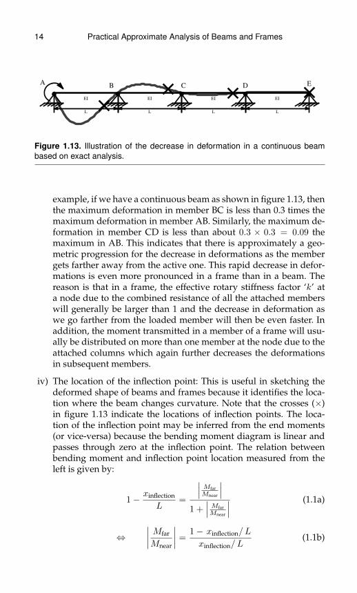
example, if we have a continuous beam as shown in figure 1.13, thenthe maximum deformation in member BC is less than 0.3 times themaximum deformation in member AB. Similarly, the maximum de-formation in member CD is less than about 0.3 × 0.3 = 0.09 themaximum in AB. This indicates that there is approximately a geo-metric progression for the decrease in deformations as the membergets farther away from the active one. This rapid decrease in defor-mations is even more pronounced in a frame than in a beam. Thereason is that in a frame, the effective rotary stiffness factor ‘k’ ata node due to the combined resistance of all the attached memberswill generally be larger than 1 and the decrease in deformation aswe go farther from the loaded member will then be even faster. Inaddition, the moment transmitted in a member of a frame will usu-ally be distributed on more than one member at the node due to theattached columns which again further decreases the deformationsin subsequent members.
iv) The location of the inflection point: This is useful in sketching thedeformed shape of beams and frames because it identifies the loca-tion where the beam changes curvature. Note that the crosses (×)in figure 1.13 indicate the locations of inflection points. The loca-tion of the inflection point may be inferred from the end moments(or vice-versa) because the bending moment diagram is linear andpasses through zero at the inflection point. The relation betweenbending moment and inflection point location measured from theleft is given by:
1− xinflection
L=
∣∣∣ MfarMnear
∣∣∣1 +
∣∣∣ MfarMnear
∣∣∣ (1.1a)
⇔∣∣∣∣ Mfar
Mnear
∣∣∣∣ =1− xinflection/L
xinflection/L(1.1b)
Practical Approximate Analysis of Beams and Frames 15
0Mapplied
(a)
0.75´4EI
LMapplied
L-xI = 0.200 L
(b)
1.00´4EI
LMapplied
L-xI = 0.222 L
(c)
1.50´4EI
LMapplied
L-xI = 0.250 L
(d)
2.00´4EI
LMapplied
L-xI = 0.267 L
(e)
¥Mapplied
L-xI = 0.333 L
(f)
Figure 1.14. Inflection points marked with × as the rotary spring stiffness in-creases (a) to (f).
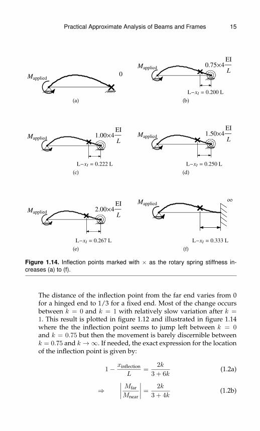
The distance of the inflection point from the far end varies from 0for a hinged end to 1/3 for a fixed end. Most of the change occursbetween k = 0 and k = 1 with relatively slow variation after k =1. This result is plotted in figure 1.12 and illustrated in figure 1.14where the the inflection point seems to jump left between k = 0and k = 0.75 but then the movement is barely discernible betweenk = 0.75 and k →∞. If needed, the exact expression for the locationof the inflection point is given by:
1− xinflection
L=
2k
3 + 6k(1.2a)
⇒∣∣∣∣ Mfar
Mnear
∣∣∣∣ =2k
3 + 4k(1.2b)

16 Practical Approximate Analysis of Beams and Frames
The above exact results are simple enough but the practitioner is ex-pected to memorize a few values from table 1.1 and use those valueswith interpolation between them rather than use the exact formulaeach time. With practice, the use of those values becomes simple andautomatic.
v) The location at which the deflection is maximum: This is mildly use-ful in sketching in the sense of knowing the general location wherethe maximum occurs. In particular, we will not be sufficiently care-ful in sketching deformations to require an accurate location for themaximum. However, this location becomes important when sketch-ing influence lines for indeterminate structures because it indicatesthe location of maximum influence in the member. The location ofthe maximum deflection always occurs closer to the near end and itsdistance to the near end monotonically decreases from about 0.42 fora hinged end to 1/3 (ie. becomes closer to the near end) for a fixedfar end.
vi) The magnitude of the maximum deflection: This will generally bemostly neglected in sketching deformations since, for clarity, we willgenerally greatly exaggerate the deformations. However, this resultis essential in approximating the influence lines of an indeterminatestructure. This maximum varies from about 0.19×θnearL for a hingedfar end and decreases monotonically to about 0.15×θnearL for a fixedend.
Aside from the above results, we note that since there are no loads onthe member then the shear force in the member is constant, the bendingmoment is linear, the slope varies parabolically and the displacement isa cubic function. In particular, the shear force is then given by:
V =(|Mnear|+ |Mfar|)
L(1.3)
The above result always applies when there are no forces applied on themember (except possibly at the ends) and we will repeatedly use it forcolumns when studying sidesway in frames.
1.4 Example: Continuous Beam withMoment Applied at Only One Node
In the first example, we consider the continuous beam shown infigure 1.15 with a unit clockwise moment applied at node C. We will beconcerned with sketching the exaggerated deformed shape of the beam

Practical Approximate Analysis of Beams and Frames 17
EI
0.5L
EI
L
EI
0.7L
EI
0.5L
EI
L
A B C D E F
Figure 1.15. A continuous beam with an applied unit clockwise moment atpoint C.
with particular attention to identify the location of the inflection points.Next we will draw an approximate bending moment diagram with themoments approximately calculated and indicated on that figure.
To sketch the continuous beam, we start with the node where theexternal moment is applied which is node C. We choose a rotation atthat node (eg. about 60◦) in the same sense (ie. clockwise) as the appliedmoment and we draw a short straight line to indicate that rotation (seefigure 1.15 at node C). That short straight line extends at both sides ofnode C because the slope must be continuous at any point where thereis no internal hinge. The exact magnitude of the rotation at C does notmatter because we are only interested in indicating the shape of the de-formations.
Next we indicate a rotation at node B using a straight line segmentin the opposite sense and at some fraction of the rotation at node C (seefigure 1.16 node B). The rotation at B is determined by considering mem-ber BC and viewing member AB as equivalent to a rotary spring at B asshown in figure 1.17a. From the previous section, we know that the ratioof rotations at B relative to C will be less than 0.5. For a quick sketch,we can take the rotation at B to be one quarter to one third that of C.Alternatively, for a more precise sketch, we calculate the k-value for therotary spring at node B in member BC to get a k-value of 1.5. This k-valueis obtained by the ratio of rotary stiffness of an isolated member AB asshown in figure 1.17b divided by the ratio of (EI/L)BC of member BC.
AB
C
D E F
Figure 1.16. Straight line extensions placed at each node.

18 Practical Approximate Analysis of Beams and Frames
B
C
k = 0.751 � H0.5 LL
1 � L
= 1.5
(a)
A
B
k = 0
(b)
C
D
k » 11 � H0.5 LL
1 � H0.7 LL» 1.4
(c)
D
E
k = 11 � H1 LL
1 � H0.5 LL= 0.5
(d)
E
F
k = ¥
(e)
Figure 1.17. Isolated members of the continuous beam shown in figure 1.15.
This more precise calculation gives a ratio of angles of 0.25 (see table 1.1)which for a rotation at C of 60◦ means a rotation of 15◦ at node B. Ofcourse, such precision in manual sketching is impractical and unneces-sary for our purposes.
To complete the rotational indications for the left side, we considermember AB as shown in figure 1.17. For that member, the rotation atnode A is known to be −0.5 that of node B and we indicate that by ashort straight line at node A as shown in figure 1.16 at node A. Thisprocess is then repeated for members CD then DE and EF. Member EFhas a fixed end and so there is no rotation at node F and we indicate thisby a short straight line at node F.
After sketching the short line segments shown in figure 1.16, wenow connect the lines using the procedures indicated in figure 1.3, 1.4and 1.5 as applicable. We also place an “×” to highlight the location ofinflection points. These are obtained from the tables based on the val-ues of the rotary spring k-values illustrated in figure 1.17. The result isshown in figure 1.18. Note that the inflection point between CD wouldbe estimated to be at 0.17L from point D based on the discussion above;

Practical Approximate Analysis of Beams and Frames 19
0.25´L 0.16´L 0.08´L 0.33´L
Figure 1.18. Sketch of the deformed shape with inflection point locations.
however, the exact result of about 0.16L is shown in the figure. All otherobtained values are the same as the exact result to within the accuracyshown in the figure (ie. 2 digits after the decimal). This difference is quiteacceptable for an approximate method.
Now, we focus our attention on sketching the bending moment di-agram. Since there are no loads on the members, the bending momentdiagrams of each member will be a straight line. Hence, we only needto calculate the values at the ends of those segments. To determine thosevalues, we start again with node C. The unit applied moment at node Cwill be resisted by both members BC and CD at their ends as shown infigure 1.19. The fraction of the applied unit moment distributed to themembers (ie. MCD and MCB) is obtained in proportion to their relativestiffness. This gives MCB ≈ (EI/L)/
((EI/L) + (EI/(0.7L)
))≈ 0.41 and
MCD ≈ (EI/(0.7L))/((EI/L) + (EI/(0.7L)
))≈ 0.59. To get a better ap-
proximation, we must use better estimates for the stiffnesses of membersBC and CD at C. The exact results are shown in figure 1.20 which agreewith the simple estimates to 2 significant digits.
Once the distributed moments at C are calculated, we proceed mem-ber by member away from node C. The bending moment at the other
MCB
MCD
Mapplied = 1
C
Figure 1.19. A continuous beam with an applied unit clockwise moment at point C.

20 Practical Approximate Analysis of Beams and Frames
0
0.139
-0.416
0.584
-0.178
0.036
-0.018
AB
C D
E
F
Figure 1.20. The bending moment diagram for the continuous beam of figure 1.15.
end of each member may either be determined by using the location ofthe inflection point or by referring back to the tables. As an exampleof using the tables, we consider calculating the moment at B of mem-ber BC. For that member, we have a k-value of 1.5 which from the tablesgives a “carry-over-moment” of 0.333; therefore, the moment at B willbe MCB × 0.333 ≈ 0.416 × 0.333 ≈ 0.139. The moments in all the othermembers may be calculated similarly or by using similar triangles whileknowing the approximate location of the inflection point. The final resultis shown in figure 1.20.
1.5 Outline of Approximate Methodfor Analyzing Structureswith No Sidesway
As the previous example shows, we can approximately analyze beamsand frames with no sidesway and with moments applied only at nodes.This is done by the following steps:
i) Distribute the applied moment onto the connected members accord-ing to their effective stiffness. Each of those effective stiffnesses maybe estimated by using table 1.1 as a guide. In any case, the error inusing a rough estimate for the stiffness (ie. EI/L of each member)will be less than 7.2% as discussed previously.
ii) Consider each member in turn starting with the members connectedto the node with the applied moment. Model that member as ahinged beam with an applied moment at one end and a rotary springat the other. By roughly estimating the stiffness of the rotary spring,we can well approximate the inflection point and the end moments.
iii) The end moments at the rotary springs are considered as appliedmoments on the nodes which are then distributed to their other con-nected members using the same procedure as step (i). These three

Practical Approximate Analysis of Beams and Frames 21
steps are then repeated until the whole structure is completed with-out requiring iteration.
iv) In case of a loop, the last member in a loop will have specifiedmoments at both ends. Its deformed shape may easily be sketchedand the bending moment is a straight line connecting the two endmoments.
Applied moments at multiple nodes is handled through superposi-tion. This means we analyze each applied moment when acting alone onthe structure and then we sum up the responses. We note that since theeffect of an applied moment decreases rapidly away from the point ofapplication (eg. figure 1.13), the moment at any node may be evaluatedby considering the superposition of the effects of only “nearby” appliedmoments. This gives good approximate results when all the applied mo-ments have comparable magnitudes. Further discussions and shortcutson how to analyze combined loads is discussed in a later section.
To proceed further, we must consider the response of loaded mem-bers. As indicated in the section on passive members, a single loadedmember in a structure with no sidesway may be handled by isolatingthe member and placing rotary springs of appropriate stiffness at eachend. Therefore, to analyze beams and frames with no sidesway and withonly one loaded member we do the following:
i) Analyze the loaded member with appropriate rotary springs at eachend. In particular, calculate the end moments at the rotary springs.
ii) Use the calculated moments at the ends of the loaded member asif they were external moments applied on the rest of the membersconnected at those ends. At that point, the rest of the structure onthe left and right of the loaded member can then be analyzed usingthe four steps detailed above.
Beams or frames with more than one loaded member may be an-alyzed by superposition. This means we analyze one loaded memberwhen acting alone on the structure and then we sum up the responsesdue to all the loaded members. Again, since the effect of applied mo-ments decreases rapidly away from the point of application, the mo-ment at any node may be evaluated by considering the superpositionof the effects of only “nearby” loaded member when end moments ofeach loaded member acting separately are comparable to end momentsof other loaded members acting separately.
Therefore, to be able to analyze any beam and frame with nosidesway, we still need to know the response of a loaded beam with ro-tary springs at each hinged end. We will consider only two special cases:

22 Practical Approximate Analysis of Beams and Frames
i) a uniformly loaded beam and ii) a concentrated or point force any-where on the beam. The point force solution may be approximately usedto analyze most other loading cases, especially at members other the theone being loaded.
1.6 Beam with a Uniform LoadA beam with a uniform load is a special type of load but it is a type thatis often encountered in applications. We first consider three special endconditions for a uniformly loaded beam as shown in figure 1.21. We willrefer to these cases as simply supported or hinged-hinged beam for fig-ure 1.21a, fixed-fixed beam for figure 1.21b and hinged-fixed beam forfigure 1.21c. The deformations and bending moment diagrams associ-ated with the special end conditions are shown in figure 1.22 and 1.23respectively. Of course, the case of fixed-hinged beam will be a mirrorimage of case figure 1.21c because we will assume that the members arehomogeneous and prismatic (ie. same properties and same cross-sectionalong the length). Because of that symmetry, the response for mirror im-age supports will be mirror image responses (eg. mirror image deforma-tions and moment diagrams).
EI
L
q
(a)
EI
L
q
(b)
EI
L
q
(c)
Figure 1.21. Three special cases for the end conditions of a uniformly loadedbeam.
(a)0.211 L 0.211 L
(b)0.250 L
(c)
Figure 1.22. Deformations of the special cases for the end conditions of a uni-formly loaded beam.
The simply supported beam in figure 1.21a has deformations withno inflection points and its curvature is always positive as seen infigure 1.22a. Consequently, its bending moment diagram is always pos-itive and its shape is as shown in figure 1.23a. This bending moment

Practical Approximate Analysis of Beams and Frames 23
qL2
8
(a)
-0.667qL
2
8
0.333qL
2
8
-0.667qL
2
8
(b)
0.563qL
2
8
-1.000qL
2
8
(c)
Figure 1.23. Moment diagrams of the special cases for the end conditions of auniformly loaded beam.
EI
L
qkL´4
EI
L
kR´4
EI
L
(a)
kL ´ 4
EI
L
kR ´ 4
EI
L
xInf Left
xInf Right
(b)
MLeft
Min max
Mright
kL ´ 4
EI
L
kR ´ 4
EI
L
(c)
Figure 1.24. Uniformly loaded beam attached to passive structures on both sides.
reaches a maximum value of qL2/8 where ‘q’ is the magnitude of theuniform load and ‘L’ is the length of the beam. By considering the gen-eral case shown in figure 1.24a, we find that this is the maximum positivemoment that can occur in any uniformly loaded beam that is attached topassive structures on both ends. Consequently, in tabulations and plotsof bending moments of a uniformly loaded beam, we will always presentthose results as ratios of that maximum moment (ie. we normalize by thatmaximum). This normalization is also useful in manual calculations be-cause i) all the dimensional values are centralized in one place and thuswe only need to do a careful dimensional calculation once and ii) weonly need to remember a few non-dimensional values between 0 and 1to get an acceptable approximation of most beams and frames with nosidesway.
The fixed-fixed beam in figure 1.21b has deformations with twoinflections points and zero slopes or rotations at each end as seen infigure 1.22b. Its bending moment diagram is as shown in figure 1.23bwhere the negative moment at the ends is twice the positive in the mid-dle. The sum of the absolute values of the positive moment in the mid-dle and negative moment at an end equals qL2/8. This is always truewhenever the rotary spring stiffnesses at the ends are the same includ-ing the limit of infinite stiffness of the fixed-fixed ends. The reason isthat we can view the symmetric end conditions as a superposition of the
24 Practical Approximate Analysis of Beams and Frames
MLeft
Min max
Mright
kL ´ 4
EI
L
kR ´ 4
EI
L
(a)
0
qL2
8
0
(b)
MleftMright
MleftMright
(c)
Figure 1.25. Superposition of moment diagrams for uniformly loaded beam.
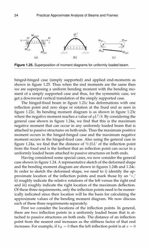
hinged-hinged case (simply supported) and applied end-moments asshown in figure 1.25. Thus when the end moments are the same thenwe are superposing a uniform bending moment with the bending mo-ment of a simply supported case and thus, for the symmetric case, weget a downward vertical translation of the simply supported case.
The hinged-fixed beam in figure 1.21c has deformations with oneinflection point and zero slope or rotation at the fixed end as seen infigure 1.22c. Its bending moment diagram is as shown in figure 1.23cwhere the negative moment reaches a value of qL2/8. By considering thegeneral case shown in figure 1.24a, we find that this is the maximumnegative moment that can occur in any uniformly loaded beam that isattached to passive structures on both ends. Thus the maximum positivemoment occurs in the hinged-hinged case and the maximum negativemoment occurs in the hinged-fixed case. Also using the general case infigure 1.24a, we find that the distance of ‘0.25L’ of the inflection pointfrom the fixed end is the farthest that an inflection point can occur in auniformly loaded beam attached to passive structures on both ends.
Having considered some special cases, we now consider the generalcase shown in figure 1.24. A representative sketch of the deformed shapeand the bending moment diagram are shown in figures 1.24b and 1.24c.In order to sketch the deformed shape, we need to i) identify the ap-proximate location of the inflection points and mark those by an ‘×,’ii) roughly indicate the relative rotations of the left versus the right endand iii) roughly indicate the right location of the maximum deflection.Of these three requirements, only the inflection points need to be numer-ically indicated since their location will be the basis for calculating theapproximate values of the bending moment diagram. We now discusseach of these three requirements separately.
First we consider the locations of the inflection points. In general,there are two inflection points in a uniformly loaded beam that is at-tached to passive structures on both ends. The distance of an inflectionpoint from the nearest end increases as the stiffness factor of that endincreases. For example, if kR = 0 then the left inflection point is at x = 0
Practical Approximate Analysis of Beams and Frames 25
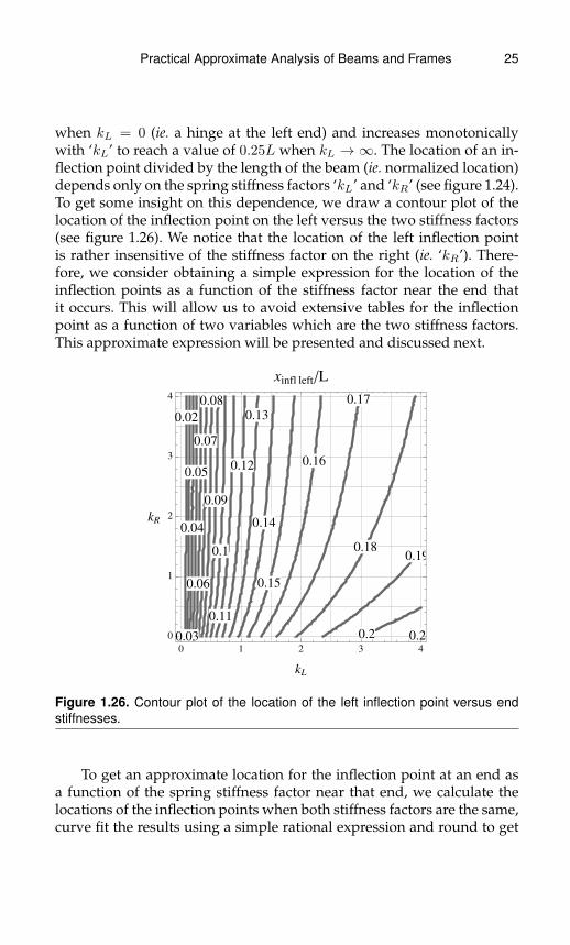
when kL = 0 (ie. a hinge at the left end) and increases monotonicallywith ‘kL’ to reach a value of 0.25L when kL → ∞. The location of an in-flection point divided by the length of the beam (ie. normalized location)depends only on the spring stiffness factors ‘kL’ and ‘kR’ (see figure 1.24).To get some insight on this dependence, we draw a contour plot of thelocation of the inflection point on the left versus the two stiffness factors(see figure 1.26). We notice that the location of the left inflection pointis rather insensitive of the stiffness factor on the right (ie. ‘kR’). There-fore, we consider obtaining a simple expression for the location of theinflection points as a function of the stiffness factor near the end thatit occurs. This will allow us to avoid extensive tables for the inflectionpoint as a function of two variables which are the two stiffness factors.This approximate expression will be presented and discussed next.
0.02
0.03
0.04
0.05
0.06
0.07
0.08
0.09
0.1
0.11
0.12
0.13
0.14
0.15
0.16
0.17
0.180.19
0.2 0.21
0 1 2 3 4
0
1
2
3
4
kL
kR
xinfl left�L
Figure 1.26. Contour plot of the location of the left inflection point versus endstiffnesses.
To get an approximate location for the inflection point at an end asa function of the spring stiffness factor near that end, we calculate thelocations of the inflection points when both stiffness factors are the same,curve fit the results using a simple rational expression and round to get
26 Practical Approximate Analysis of Beams and Frames
decreasing kR
Range: H0,¥L
0 1 2 3 4
k0.
0.05
0.1
0.15
0.2
0.25
xI �L
0.01 0.1 1 10 100 100010
4
0.
0.025
0.05
0.075
0.1
0.125
0.15
0.175
0.2
0.225
0.25
Inflection point: Exact vs approximate
Figure 1.27. Comparsion of inflection point location between exact (solid thinlines) and approximate (dashed thick line).
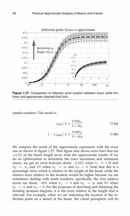
simple numbers. The result is:
xIleft/L ≈0.92kL3 + 4kL
(1.4a)
1− xIright/L ≈ 0.92kR
3 + 4kR(1.4b)
We compare the result of the approximate expression with the exactone as shown in figure 1.27. That figure also shows error bars that are±2.5% of the beam length away from the approximate results. If wedo an optimization to determine the exact maximum and minimumerrors, we get an error between about −2.34% when kL ≈ 1.76 andkR → ∞, and 2% when kL → ∞ and kR = 0. Note that this is apercentage error which is relative to the length of the beam while therelative error relative to the location would be higher because we aresometimes dealing with small numbers; specifically, the true relativeerrors are about −38% when kL → 0 and kR → ∞ and 8% whenkL → ∞ and kR = 0. For the purposes of sketching and obtaining thebending moment diagram, it is the error relative to the length that isrelevant. For example, when we are indicating the location of the in-flection point on a sketch of the beam, the visual perception will be
Practical Approximate Analysis of Beams and Frames 27
relative to the length of the beam. In that regards,±2.5% would be barelydiscernible and about the thickness of the line drawn. Moreover, in amanual sketch small features will be perceived relative to the lengthof the beam and, in particular, the error in a manual indication of theinflection points will usually exceed an error of ±2.5% relative to thelength.
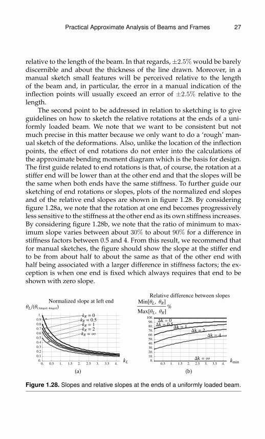
The second point to be addressed in relation to sketching is to giveguidelines on how to sketch the relative rotations at the ends of a uni-formly loaded beam. We note that we want to be consistent but notmuch precise in this matter because we only want to do a ‘rough’ man-ual sketch of the deformations. Also, unlike the location of the inflectionpoints, the effect of end rotations do not enter into the calculations ofthe approximate bending moment diagram which is the basis for design.The first guide related to end rotations is that, of course, the rotation at astiffer end will be lower than at the other end and that the slopes will bethe same when both ends have the same stiffness. To further guide oursketching of end rotations or slopes, plots of the normalized end slopesand of the relative end slopes are shown in figure 1.28. By consideringfigure 1.28a, we note that the rotation at one end becomes progressivelyless sensitive to the stiffness at the other end as its own stiffness increases.By considering figure 1.28b, we note that the ratio of minimum to max-imum slope varies between about 30% to about 90% for a difference instiffness factors between 0.5 and 4. From this result, we recommend thatfor manual sketches, the figure should show the slope at the stiffer endto be from about half to about the same as that of the other end withhalf being associated with a larger difference in stiffness factors; the ex-ception is when one end is fixed which always requires that end to beshown with zero slope.
0. 0.5 1. 1.5 2. 2.5 3. 3.5 4.kL
0.
0.1
0.2
0.3
0.4
0.5
0.6
0.7
0.8
0.9
1.
ΘL�HΘL hinged-hingedLNormalized slope at left end
kR = ¥
kR = 2
kR = 1
kR = 0.5
kR = 0
(a)0.5 1. 1.5 2. 2.5 3. 3.5 4.
kmin0.
10.
20.
30.
40.
50.
60.
70.
80.
90.
100.
Min@ΘL, ΘRD
Max@ΘL, ΘRD%
Relative difference between slopes
Dk = ¥
Dk = 4
Dk = 2Dk = 1
Dk = 0.5Dk = 0
(b)
Figure 1.28. Slopes and relative slopes at the ends of a uniformly loaded beam.
28 Practical Approximate Analysis of Beams and Frames
0.001 0.01 0.1 1 10 100 1000kL
0.2
0.4
0.6
0.8
1.0
xat max�LLocation of maximum displacement
decreasing kR
Range: H0,¥L
(a)
decreasing kR
kR = 0
kR = 0.5kR = 1
kR = 2kR = 4
kR = ¥
0. 0.5 1. 1.5 2. 2.5 3. 3.5 4.kL
0.
0.1
0.2
0.3
0.4
0.5
0.6
0.7
0.8
0.9
1.
∆max�∆hinges
Normalized maximum displacement
(b)
Figure 1.29. Location and magnitude of the maximum displacement in a uniformlyloaded beam.
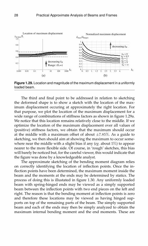
The third and final point to be addressed in relation to sketchingthe deformed shape is to show a sketch with the location of the max-imum displacement occuring at approximately the right location. Forthat purpose, we plot the location of the maximum displacement for awide range of combinations of stiffness factors as shown in figure 1.29a.We notice that this location remains relatively close to the middle. If weoptimize the location of the maximum displacement over all values of(positive) stiffness factors, we obtain that the maximum should occurat the middle with a maximum offset of about ±7.85%. As a guide tosketching, we then should aim at showing the maximum to occur some-where near the middle with a slight bias if any (eg. about 5%) to appearnearer to the more flexible side. Of course, in ‘rough’ sketches, this biaswill barely be noticed but, for the careful viewer, this would indicate thatthe figure was done by a knowledgeable analyst.
The approximate sketching of the bending moment diagram relieson correctly identifying the location of inflection points. Once the in-flection points have been determined, the maximum moment inside thebeam and the moments at the ends may be determined by statics. Theprocess of doing this is illustated in figure 1.30. Any uniformly loadedbeam with spring-hinged ends may be viewed as a simply supportedbeam between the inflection points with two end pieces on the left andright. The reason is that the bending moment at inflection points is zeroand therefore these locations may be viewed as having hinged sup-ports on top of the remaining parts of the beam. The simply supportedbeam and each of the ends may then be simply analyzed to obtain themaximum internal bending moment and the end moments. These are

Practical Approximate Analysis of Beams and Frames 29
q
xIL Leff L-xIR
⇔
q
xIL Leff L-xIR
analyzed asq
Leff
and
q
xIL
qLeff�2 and
q
L-xIR
qLeff�2
Figure 1.30. Obtaining moment diagram by knowing the location of the inflectionpoints.
given by:
Min max =qL2
effective
8(1.5a)
Mleft =qLeffective
2× xIL +
qx2IL
2=qxIL (Leff + xIL)
2(1.5b)
Mright =qLeffective
2× (L− xIR) +
q (L− xIR) 2
2
=q (L− xIR) (Leff + L− xIR)
2(1.5c)
In addition to the above, we also deduce that the location of the max-imum internal bending moment is at the center of the effective sim-ply supported beam between the inflection points (ie. at (xIL + xIR)/ 2).Finally, we can sketch the bending moment diagram. This diagram mustbe a parabola because, from elementary mechanics of materials, the sec-ond derivative of the moment is a constant equal to the uniform dis-tributed load. In addition, this parabola has a negative curvature andmust pass through the inflection points which are locations where thebending moment is zero. Finally, after drawing such a parabola, we canmark the maximum internal bending moment and end moments fromthe values calculated using formulas 1.5a to 1.5c).

30 Practical Approximate Analysis of Beams and Frames
kR = 0
kR = 0.25
kR = 0.5
kR = 1
kR = 2
kR = 4
kR = ¥
0.5 1. 1.5 2. 2.5 3. 3.5 4.kL
-8
-6
-4
-2
0
2
4
6
8
DMleft�HqL2�8L %
Mleft: Exact vs approximate
(a)
kR = 0
kR = 0.25
kR = 0.5
kR = 1
kR = 2kR = 4kR = ¥
0.5 1. 1.5 2. 2.5 3. 3.5 4.kL
-4
-3
-2
-1
0
1
2
3
4
DMin max�HqL2�8L %
Min max: Exact vs approximate
(b)
Figure 1.31. Error between bending moments obtained from exact versus ap-proximate location of inflection points.
Of course, the errors in the calculated bending moments are relatedto the errors in the approximate locations of the inflection points. If weuse formula 1.4a and 1.4b to estimate the location of inflection pointsand we plot the error at the left end (right is analogous) and at the innermaximum bending moment then we get the results shown in figure 1.31.Note that those percent errors are relative to the maximum moment ina simply supported beam. For the left end moment (right end is equiv-alent), by optimizing the difference between the approximate and exactresults, we find that the maximum error is between−7.23% which occurswhen kL ≈ 1.33 and kR → ∞ and 8% which occurs when kL → ∞ andkR = 0. Alternatively, we can characterize the relative error by constrain-ing the smallest (absolute) value of the left end moment. Specifically,if the approximately calculated left end moment is (in absolute value)greater than 0.2 qL2
/8 then the maximum relative error is between−8%
which occurs when kL → ∞ and kR = 0 and 31.7% which occurs whenkL ≈ 0.295 and kR →∞.
For the inner maximum moment, by optimizing the difference be-tween the approximate and exact results, we find that the maximum er-ror relative to qL2
/8 is between −4.17% which occurs when kL → ∞
and kR →∞ and 3.04% which occurs when kL →∞ and kR = 0 (or viceversa). Alternatively, we can characterize the relative error of the innermaximum moment. Specifically, the relative error of the inner maximummoment is between about −6.77% which occurs when kL ≈ 1.32 andkR → ∞ and about 5.39% which occurs when kL → ∞ and kR = 0.The approximate expression for the inner maximum moment has gen-erally lower percent error than the one for the end moment because itsvalue never goes below about 0.33 qL2
/8 while the end moments can
reach zero. In any case, these results show that this approximate analysis
Practical Approximate Analysis of Beams and Frames 31
gives sufficient accuracy for preliminary design or to check the output ofcomputer calculations.
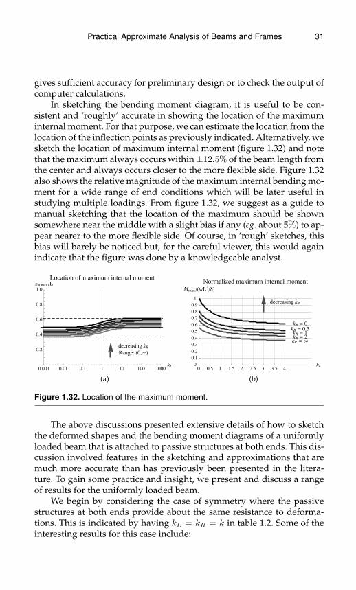
In sketching the bending moment diagram, it is useful to be con-sistent and ‘roughly’ accurate in showing the location of the maximuminternal moment. For that purpose, we can estimate the location from thelocation of the inflection points as previously indicated. Alternatively, wesketch the location of maximum internal moment (figure 1.32) and notethat the maximum always occurs within±12.5% of the beam length fromthe center and always occurs closer to the more flexible side. Figure 1.32also shows the relative magnitude of the maximum internal bending mo-ment for a wide range of end conditions which will be later useful instudying multiple loadings. From figure 1.32, we suggest as a guide tomanual sketching that the location of the maximum should be shownsomewhere near the middle with a slight bias if any (eg. about 5%) to ap-pear nearer to the more flexible side. Of course, in ‘rough’ sketches, thisbias will barely be noticed but, for the careful viewer, this would againindicate that the figure was done by a knowledgeable analyst.
0.001 0.01 0.1 1 10 100 1000kL
0.2
0.4
0.6
0.8
1.0
xat max�LLocation of maximum internal moment
decreasing kR
Range: H0,¥L
(a)
decreasing kR
kR = ¥
kR = 2kR = 1
kR = 0.5
kR = 0
0. 0.5 1. 1.5 2. 2.5 3. 3.5 4.kL0.
0.1
0.2
0.3
0.4
0.5
0.6
0.7
0.8
0.9
1.
Mmax�HwL2�8L
Normalized maximum internal moment
(b)
Figure 1.32. Location of the maximum moment.
The above discussions presented extensive details of how to sketchthe deformed shapes and the bending moment diagrams of a uniformlyloaded beam that is attached to passive structures at both ends. This dis-cussion involved features in the sketching and approximations that aremuch more accurate than has previously been presented in the litera-ture. To gain some practice and insight, we present and discuss a rangeof results for the uniformly loaded beam.
We begin by considering the case of symmetry where the passivestructures at both ends provide about the same resistance to deforma-tions. This is indicated by having kL = kR = k in table 1.2. Some of theinteresting results for this case include:

32 Practical Approximate Analysis of Beams and Frames
Table 1.2. Uniformly Loaded Beam: Symmetric Spring Resistance.
EI
L
qk
EI
L
kEI
L
k xInfl/L at left 1− xInf/L at right −Mleft/qL2
8−Mright/
qL2
8Min max/
qL2
8
0.000 0.000 0.000 0.000 0.000 1.0000.500 0.092 0.092 0.333 0.333 0.6670.750 0.113 0.113 0.400 0.400 0.6001.000 0.127 0.127 0.444 0.444 0.5561.500 0.146 0.146 0.500 0.500 0.5002.000 0.158 0.158 0.533 0.533 0.4673.000 0.173 0.173 0.571 0.571 0.4294.000 0.181 0.181 0.593 0.593 0.407∞ 0.211 0.211 0.667 0.667 0.333
i) k = 0 (simply supported): This gives the largest possible positivemoment for a uniformly loaded beam attached to passive structuresat both ends.
ii) k → ∞ (fixed-fixed): The negative moments at the ends are twicethose at the middle. Also, the inflection points are the farthest intothe beam of any symmetric case and occur at a distance of about0.21L from each end.
iii) k = 1: This is the value we would use to approximate any non-terminal span (ie. not occuring at either end) of a continuous beamof equal spans. In this case, the internal maximum moment is about0.56 that of the simply supported case and the negative moments atthe ends are about 0.44. Also, inflection points are at a distance ofabout 0.13L from the ends.
iv) k = 1.5: At this value, the negative and positive moments are equalin absolute values. If we minimize the maximum absolute value ofbending moments in a uniformly loaded beam for any uniformlyloaded beam attached to passive supports then we get this case.For a material whose yield in tension is the same as in compres-sion (eg. steel), this constitutes the end supports that would allowthe largest uniform load to be supported before failure.
Three examples of symmetric cases for the exact deformations andexact bending moment diagrams are shown in figures 1.33 and 1.34

Practical Approximate Analysis of Beams and Frames 33
1 ´ 4
EI
L
1 ´ 4
EI
L
0.127 L 0.127 L
(a)
2 ´ 4
EI
L
2 ´ 4
EI
L
0.158 L 0.158 L
(b)
4 ´ 4
EI
L
4 ´ 4
EI
L
0.181 L 0.181 L
(c)
Figure 1.33. Deformed shape of selected cases of unifomly loaded beam withsymmetric supports.
respectively. We note that the negative curvature part of the deforma-tion is barely discernible and thus the importance of indicating (eg. inthe figures with an ‘×’) the location of the inflection points. Aside fromthe magnitude of the deformations and the location of the inflectionpoints, the deformation shapes for the symmetric cases are about thesame over a wide range of stiffness factors. They all look somewhat likeparabolas with relatively short pieces at each end having slight negativecurvatures.
The moment diagrams shown in figure 1.34 all have the same shapebut with a vertical downward shift that increases with the stiffness factor‘k.’ Of course, this causes the bending moments to intersect the zero lineat different locations which coincide with the location of the inflectionpoints.
-0.444
qL2
8
0.556
qL2
8
-0.444
qL2
8
1 ´ 4
EI
L
1 ´ 4
EI
L
(a)
-0.533
qL2
8
0.467
qL2
8
-0.533
qL2
8
2 ´ 4
EI
L
2 ´ 4
EI
L
(b)
-0.593
qL2
8
0.407
qL2
8
-0.593
qL2
8
4 ´ 4
EI
L
4 ´ 4
EI
L
(c)
Figure 1.34. Moment diagrams of selected cases of uniformly loaded beam withsymmetric supports.
In comparison with the symmetric case, we first present a few caseswhere the ends have unequal stiffness factors but neither end is a hingeor a fixed end (see figures 1.35 and 1.36). From figure 1.35, we noticethat, aside from the location of inflection points, the shapes are still sim-ilar to those of the symmetric cases. In particular, in manual sketches,they would be indistinguishable. Therefore, we only need to learn howto manually sketch one prototypical shape when neither end is a hingeor a fixed end.

34 Practical Approximate Analysis of Beams and Frames
1 ´ 4
EI
L
2 ´ 4
EI
L
0.121 L0.165 L
(a)
1 ´ 4
EI
L
4 ´ 4
EI
L
0.117 L0.193 L
(b)
2 ´ 4
EI
L
4 ´ 4
EI
L
0.153 L 0.187 L
(c)
Figure 1.35. Deformed shape of selected cases of uniformly loaded beam withnon-symmetric supports.
-0.406
qL2
8
0.509
qL2
8
-0.580
qL2
8
1 ´ 4
EI
L
2 ´ 4
EI
L
(a)
-0.376
qL2
8
0.476
qL2
8
-0.684
qL2
8
1 ´ 4
EI
L
4 ´ 4
EI
L
(b)
-0.497
qL2
8
0.436
qL2
8
-0.633
qL2
8
2 ´ 4
EI
L
4 ´ 4
EI
L
(c)
Figure 1.36. Moment diagrams of selected cases of uniformly loaded beam withnon-symmetric supports.
The bending moment diagrams (figures 1.36) for the unsymmetriccase differ from those of the symmetric ones only by their unequal val-ues at the ends. As noted before and indicated in figure 1.32a, the loca-tion of the maximum does not move much from the middle of the beam.Therefore, as a guide to manual sketching, we suggest first marking thelocation of the negative moments at the ends and the positive maximuminternal moment somewhere near the middle and then drawing an in-verted parabola that passes through those points. Also, as much as pos-sible in a manual sketch, the location of zero bending moment shouldcoincide with those of the inflection points.
After considering cases of the uniformly loaded beam where the endconditions are neither a hinge nor a fixed end, we now consider each ofthose possibilites. The cases where each end is either a hinge or a fixedend have been discussed and are shown in figures 1.22 and 1.23 for thedeformed shape and bending moment diagrams respectively. The de-formed shape of the simply supported case looks similar to the casesshown in figures 1.33 and 1.35 except that there are no inflection points.The new feature in the deformed shape only occurs at a fixed end; inthat case, there is a clear negative curvature portion and the slope iszero at the fixed end. Those features can be manually drawn using a

Practical Approximate Analysis of Beams and Frames 35
Table 1.3. Uniformly Loaded Beam: One End Hinged.
EI
L
qk
EI
L
k xInfl/L at left 1− xInf/L at right −Mleft/qL2
8−Mright/
qL2
8Min max/
qL2
8
0.000 0.000 0.000 0.000 0.000 1.0000.500 0.000 0.100 0.000 0.400 0.8100.750 0.000 0.125 0.000 0.500 0.7661.000 0.000 0.143 0.000 0.571 0.7351.500 0.000 0.167 0.000 0.667 0.6942.000 0.000 0.182 0.000 0.727 0.6693.000 0.000 0.200 0.000 0.800 0.6404.000 0.000 0.211 0.000 0.842 0.623∞ 0.000 0.250 0.000 1.000 0.563
technique similar to the one outlined in the introduction and illustratedin figure 1.3. Based on extensive viewing of exact test cases, we notethat a clear negative curvature portion of the curve near a rotary springsupport only gradually occurs as the stiffness factor increases beyondabout 10 to 20. Such a stiffness factor is very high and may be practicallyconsidered as equivalent to a fixed end. Finally, the bending moment di-agrams for these special cases are similar to those shown in figures 1.34and 1.36 except that the end with the hinge has zero moment and maybe manually sketched in the same way.
We now consider the case where one end is a hinge and the other isconnected to a passive structure. This is indicated by having kL = 0 andkR = k in table 1.3. Some of the interesting results for this case include:
i) k = 0 (simply supported): This was discussed previously.
ii) k →∞ (hinged-fixed): This gives the maximum negative moment thatcan occur in any uniformly loaded beam that is attached to passivestructures on both ends. Interestingly, that maxium equals (in absolutevalue) the maximum possible positive moment. In addition, this casealso gives the largest distance that an inflection point can move awayfrom an end in a uniformly loaded beam attached to passive structuresat both ends. That distance is at 0.25L from the fixed end.
iii) k = 1: This is the value we would use to approximate a hinged end-span of a continuous beam of equal spans. In this case, the normalizedinternal maximum moment is about 0.74 that of the simply supportedcase and the normalized negative moments at the spring-end is about

36 Practical Approximate Analysis of Beams and Frames
0.57. Also, the inflection point is at a distance of about 0.14L from thespring end.
iv) k ≈ 1.641 (not shown): At this value, the normalized negative andpositive moments are both equal to about 0.686 in absolute value. Ifwe minimize the maximum absolute value of bending moments in auniformly loaded beam for any uniformly loaded beam attached toa hinge at one end and a passive support at the other, then we getthis case. For a material whose yield in tension is the same as in com-pression (eg. steel), this constitutes the end support at the right with ahinged left end support that would allow the largest uniform load tobe supported before failure.
Three examples of hinged-spring cases of table 1.3 for the ex-act deformations and exact bending moment diagrams are shown infigures 1.37 and 1.38 respectively. We note that the deformations looksimilar to those of the symmetric cases except that there is no negativecurvature at the hinged end which is indicated by putting a ‘×’ at thehinge. Again, we must indicate the location of the inflection point whichmay be approximately calculated using formulas 1.4 or exactly obtainedfrom table 1.3.
1 ´ 4
EI
L
0.143 L
(a)
2 ´ 4
EI
L
0.182 L
(b)
4 ´ 4
EI
L
0.211 L
(c)
Figure 1.37. Deformed shape of selected cases of uniformly loaded beam withhinge-spring supports.
0
0.735
qL2
8
-0.571
qL2
8
1 ´ 4
EI
L
(a)
0
0.669
qL2
8
-0.727
qL2
8
2 ´ 4
EI
L
(b)
0
0.623
qL2
8
-0.842
qL2
8
4 ´ 4
EI
L
(c)
Figure 1.38. Moment diagrams of selected cases of uniformly loaded beam withhinge-spring supports.
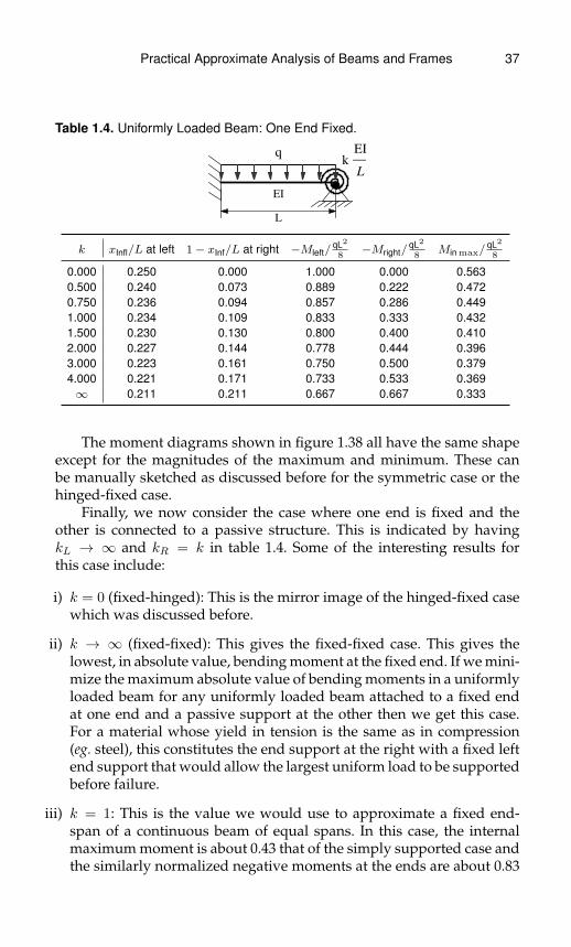
Practical Approximate Analysis of Beams and Frames 37
Table 1.4. Uniformly Loaded Beam: One End Fixed.
EI
L
qk
EI
L
k xInfl/L at left 1− xInf/L at right −Mleft/qL2
8−Mright/
qL2
8Min max/
qL2
8
0.000 0.250 0.000 1.000 0.000 0.5630.500 0.240 0.073 0.889 0.222 0.4720.750 0.236 0.094 0.857 0.286 0.4491.000 0.234 0.109 0.833 0.333 0.4321.500 0.230 0.130 0.800 0.400 0.4102.000 0.227 0.144 0.778 0.444 0.3963.000 0.223 0.161 0.750 0.500 0.3794.000 0.221 0.171 0.733 0.533 0.369∞ 0.211 0.211 0.667 0.667 0.333
The moment diagrams shown in figure 1.38 all have the same shapeexcept for the magnitudes of the maximum and minimum. These canbe manually sketched as discussed before for the symmetric case or thehinged-fixed case.
Finally, we now consider the case where one end is fixed and theother is connected to a passive structure. This is indicated by havingkL → ∞ and kR = k in table 1.4. Some of the interesting results forthis case include:
i) k = 0 (fixed-hinged): This is the mirror image of the hinged-fixed casewhich was discussed before.
ii) k → ∞ (fixed-fixed): This gives the fixed-fixed case. This gives thelowest, in absolute value, bending moment at the fixed end. If we mini-mize the maximum absolute value of bending moments in a uniformlyloaded beam for any uniformly loaded beam attached to a fixed endat one end and a passive support at the other then we get this case.For a material whose yield in tension is the same as in compression(eg. steel), this constitutes the end support at the right with a fixed leftend support that would allow the largest uniform load to be supportedbefore failure.
iii) k = 1: This is the value we would use to approximate a fixed end-span of a continuous beam of equal spans. In this case, the internalmaximum moment is about 0.43 that of the simply supported case andthe similarly normalized negative moments at the ends are about 0.83
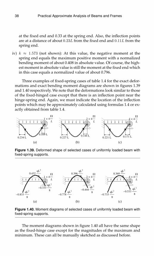
38 Practical Approximate Analysis of Beams and Frames
at the fixed end and 0.33 at the spring end. Also, the inflection pointsare at a distance of about 0.23L from the fixed end and 0.11L from thespring end.
iv) k ≈ 1.573 (not shown): At this value, the negative moment at thespring end equals the maximum positive moment with a normalizedbending moment of about 0.408 in absolute value. Of course, the high-est moment in absolute value is still the moment at the fixed end whichin this case equals a normalized value of about 0.796.
Three examples of fixed-spring cases of table 1.4 for the exact defor-mations and exact bending moment diagrams are shown in figures 1.39and 1.40 respectively. We note that the deformations look similar to thoseof the fixed-hinged case except that there is an inflection point near thehinge-spring end. Again, we must indicate the location of the inflectionpoints which may be approximately calculated using formulas 1.4 or ex-actly obtained from table 1.4.
1 ´ 4
EI
L
0.234 L
0.109 L
(a)
2 ´ 4
EI
L
0.227 L0.144 L
(b)
4 ´ 4
EI
L
0.221 L 0.171 L
(c)
Figure 1.39. Deformed shape of selected cases of uniformly loaded beam withfixed-spring supports.
-0.833
qL2
8
0.432
qL2
8
-0.333
qL2
8
1 ´ 4
EI
L
(a)
-0.778
qL2
8
0.396
qL2
8
-0.444
qL2
8
2 ´ 4
EI
L
(b)
-0.733
qL2
8
0.369
qL2
8
-0.533
qL2
8
4 ´ 4
EI
L
(c)
Figure 1.40. Moment diagrams of selected cases of uniformly loaded beam withfixed-spring supports.
The moment diagrams shown in figure 1.40 all have the same shapeas the fixed-hinge case except for the magnitudes of the maximum andminimum. These can all be manually sketched as discussed before.
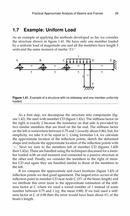
Practical Approximate Analysis of Beams and Frames 39
1.7 Example: Uniform LoadAs an example of applying the methods developed so far, we considerthe structure shown in figure 1.41. We have only one member loadedby a uniform load of magnitude one and all the members have length 5units and the same moment of inertia ‘EI .’
EI
5
EI
5
EI
5
EI
5
EI
5
1
A B C D E
F
Figure 1.41. Example of a structure with no sidesway and one member uniformlyloaded.
As a first step, we decompose the structure into components (fig-ure 1.42). We start with member CD (figure 1.42c). The stiffness factor onthe right is exactly 2 because the resistance on that side is provided bytwo similar members that are fixed on the far end. The stiffness factoron the left is somewhere between 0.75 and 1 (exactly about 0.86), but, forsimplicity, we take it to be equal to 1. Using formulas 1.4, we calculatethe approximate location of the inflection points, sketch the deformedshape and indicate the approximate location of the inflection points with‘×.’ Next we turn to the members left of member CD (figures 1.42bthen 1.42a). These are handled using the techniques discussed for a mem-ber loaded with an end moment and connected to a passive structure atthe other end. Finally, we consider the members to the right of mem-ber CD and again they are handled similar to those of the members tothe left.
If we compare the approximate and exact locations (figure 1.43) ofinflection points we find good agreement. The largest error occurs at theinflection point in member CD near node C (9% of the beam length) andwe attribute this error more to the approximate estimation of the stiff-ness factor at C where we used a round number of 1 instead of somenumber between 0.75 and 1 (eg. the mean 0.88). If we had used a stiff-ness factor at C of 0.88 then the error would have been about 6% of thebeam’s length.
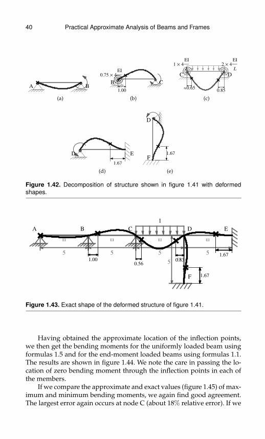
40 Practical Approximate Analysis of Beams and Frames
A B
(a)
0.75 ´ 4
EI
L
1.00
B C
(b)
1 ´ 4
EI
L
2 ´ 4
EI
L
»0.650.85
C D
(c)
1.67
D E
(d)
1.67
D
F
(e)
Figure 1.42. Decomposition of structure shown in figure 1.41 with deformedshapes.
EI
5
EI
5
EI
5
EI
5
EI
5
1
A B C D E
F
1.000.56
0.83
1.67
1.67
Figure 1.43. Exact shape of the deformed structure of figure 1.41.
Having obtained the approximate location of the inflection points,we then get the bending moments for the uniformly loaded beam usingformulas 1.5 and for the end-moment loaded beams using formulas 1.1.The results are shown in figure 1.44. We note the care in passing the lo-cation of zero bending moment through the inflection points in each ofthe members.
If we compare the approximate and exact values (figure 1.45) of max-imum and minimum bending moments, we again find good agreement.The largest error again occurs at node C (about 18% relative error). If we
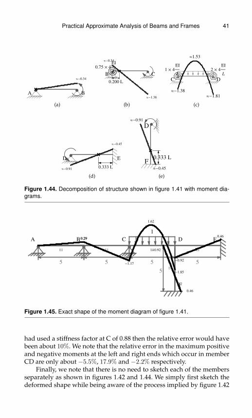
Practical Approximate Analysis of Beams and Frames 41
»-0.34
A B
(a)
0.75 ´ 4
EI
L
0.200 L
»-1.38
»-0.34
B C
(b)
»-1.38
»1.53
»-1.81
1 ´ 4
EI
L
2 ´ 4
EI
L
C D
(c)
0.333 L»-0.91
»-0.45
D E
(d)
0.333 L
»-0.91
»-0.45
D
F
(e)
Figure 1.44. Decomposition of structure shown in figure 1.41 with moment dia-grams.
EI
5
EI
5
EI
5
EI
5
EI
5
1
A B C D E
F
0.290.29
-1.17
1.62
-1.85
-0.92
0.46
-0.92
0.46
Figure 1.45. Exact shape of the moment diagram of figure 1.41.
had used a stiffness factor at C of 0.88 then the relative error would havebeen about 10%. We note that the relative error in the maximum positiveand negative moments at the left and right ends which occur in memberCD are only about −5.5%, 17.9% and −2.2% respectively.
Finally, we note that there is no need to sketch each of the membersseparately as shown in figures 1.42 and 1.44. We simply first sketch thedeformed shape while being aware of the process implied by figure 1.42
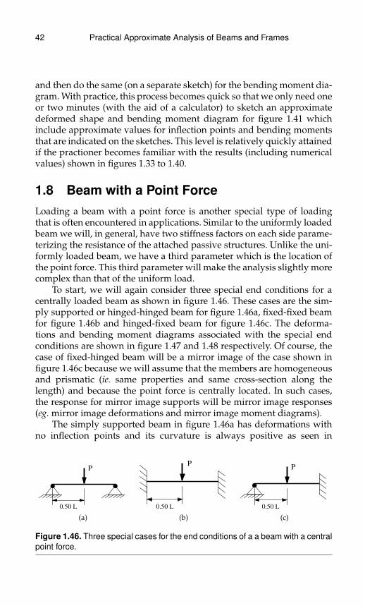
42 Practical Approximate Analysis of Beams and Frames
and then do the same (on a separate sketch) for the bending moment dia-gram. With practice, this process becomes quick so that we only need oneor two minutes (with the aid of a calculator) to sketch an approximatedeformed shape and bending moment diagram for figure 1.41 whichinclude approximate values for inflection points and bending momentsthat are indicated on the sketches. This level is relatively quickly attainedif the practioner becomes familiar with the results (including numericalvalues) shown in figures 1.33 to 1.40.
1.8 Beam with a Point ForceLoading a beam with a point force is another special type of loadingthat is often encountered in applications. Similar to the uniformly loadedbeam we will, in general, have two stiffness factors on each side parame-terizing the resistance of the attached passive structures. Unlike the uni-formly loaded beam, we have a third parameter which is the location ofthe point force. This third parameter will make the analysis slightly morecomplex than that of the uniform load.
To start, we will again consider three special end conditions for acentrally loaded beam as shown in figure 1.46. These cases are the sim-ply supported or hinged-hinged beam for figure 1.46a, fixed-fixed beamfor figure 1.46b and hinged-fixed beam for figure 1.46c. The deforma-tions and bending moment diagrams associated with the special endconditions are shown in figure 1.47 and 1.48 respectively. Of course, thecase of fixed-hinged beam will be a mirror image of the case shown infigure 1.46c because we will assume that the members are homogeneousand prismatic (ie. same properties and same cross-section along thelength) and because the point force is centrally located. In such cases,the response for mirror image supports will be mirror image responses(eg. mirror image deformations and mirror image moment diagrams).
The simply supported beam in figure 1.46a has deformations withno inflection points and its curvature is always positive as seen in
P
0.50 L
(a)
P
0.50 L
(b)
P
0.50 L
(c)
Figure 1.46. Three special cases for the end conditions of a a beam with a centralpoint force.
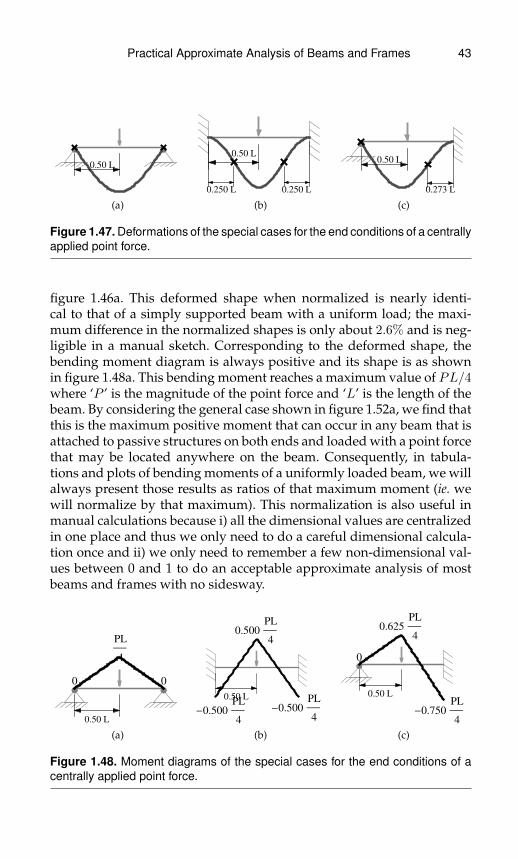
Practical Approximate Analysis of Beams and Frames 43
0.50 L
(a)0.250 L 0.250 L
0.50 L
(b)0.273 L
0.50 L
(c)
Figure 1.47. Deformations of the special cases for the end conditions of a centrallyapplied point force.
figure 1.46a. This deformed shape when normalized is nearly identi-cal to that of a simply supported beam with a uniform load; the maxi-mum difference in the normalized shapes is only about 2.6% and is neg-ligible in a manual sketch. Corresponding to the deformed shape, thebending moment diagram is always positive and its shape is as shownin figure 1.48a. This bending moment reaches a maximum value of PL/4where ‘P ’ is the magnitude of the point force and ‘L’ is the length of thebeam. By considering the general case shown in figure 1.52a, we find thatthis is the maximum positive moment that can occur in any beam that isattached to passive structures on both ends and loaded with a point forcethat may be located anywhere on the beam. Consequently, in tabula-tions and plots of bending moments of a uniformly loaded beam, we willalways present those results as ratios of that maximum moment (ie. wewill normalize by that maximum). This normalization is also useful inmanual calculations because i) all the dimensional values are centralizedin one place and thus we only need to do a careful dimensional calcula-tion once and ii) we only need to remember a few non-dimensional val-ues between 0 and 1 to do an acceptable approximate analysis of mostbeams and frames with no sidesway.
0
PL
4
0
0.50 L
(a)
-0.500PL
4
0.500PL
4
-0.500PL
4
0.50 L
(b)
0
0.625PL
4
-0.750PL
4
0.50 L
(c)
Figure 1.48. Moment diagrams of the special cases for the end conditions of acentrally applied point force.

44 Practical Approximate Analysis of Beams and Frames
The fixed-fixed beam in figure 1.46b has deformations with two in-flections points and zero slopes or rotations at each end as seen in fig-ure 1.47b. Again this deformed shape is similar to the equivalent uni-formly loaded beam but is slightly sharper in shape with a maximumdifference in the normalized shapes of only 6.25%; this is again negligiblein a manual sketch. Corresponding to the deformed shape, the bendingmoment diagram is as shown in figure 1.48b where the negative momentat the ends is the same as the positive one in the middle; this is to be con-trasted with a uniformly loaded beam where the negative moments atthe ends are twice the positive moment in the middle. The sum of theabsolute values of the positive moment in the middle and negative mo-ment at an end equals ‘PL/4.’ This is always true for central loading andwhenever the rotary spring stiffnesses at the ends are the same includingthe limit of infinite stiffness of the fixed-fixed ends. The reason is that wecan view the symmetric end conditions as a superposition of the hinged-hinged case (simply supported) and of applied equal end-moments asshown in figure 1.53. Thus when the end moments are the same, thenwe are superposing a uniform bending moment with the bending mo-ment of a simply supported case. This then implies that any symmetricsupport case will have a bending moment diagram that is a downwardvertical translation of the bending moment diagram of the simply sup-ported case.
The hinged-fixed beam in figure 1.46c has deformations with oneinflection point and zero slope or rotation at the fixed end as seen infigure 1.47c. Again this deformed shape is similar to the equivalent uni-formly loaded beam but is slightly sharper with a maximum difference inthe normalized shapes of only 7.8%; this is again negligible in a manualsketch. Its bending moment diagram is as shown in figure 1.48c wherethe negative moment reaches a value of 0.75PL/4. By considering thegeneral case shown in figure 1.52a, we find that this is not the maxi-mum negative moment that can occur in a beam that is attached to pas-sive structures on both ends and having a point force somewhere alongits span. That maximum does occurs for a hinged-fixed case but withthe location of the point force being at about 0.423L distance from thefixed end (ie. 0.577L distance from the hinged end). The correspondingmaximum negative moment is about 0.77PL/4. Also using the generalcase in figure 1.52a, we find that the maximum distance of an inflectionpoint from its nearest end also occurs for the hinge-fixed case and hasa value of one-third the beam length (≈ 0.333L). This case occurs inthe limit as the point force approaches but does not reach the hingedend. We note that this limiting case is then equivalent to that of a beamwith an infinitesimal moment applied at one end and a fixed end at theother.

Practical Approximate Analysis of Beams and Frames 45
P
0.25 L
(a)
P
0.25 L
(b)
P
0.25 L
(c)
P
0.75 L
(d)
Figure 1.49. Four special cases for the end conditions of a beam with a non-central point force.
Having considered centrally loaded cases with special end condi-tions, we now consider similar special end conditions but with non-centrally loaded cases as shown in figure 1.49. These are the simply sup-ported beam with a load at a quarter the length from one support shownin figure 1.49a, the fixed-fixed beam with a load at a quarter the lengthfrom one support shown in figure 1.49b and the hinged-fixed beam witha load at a quarter and at three-quarters the length from the hinged endas shown figures 1.49c and 1.49d respectively.
What is interesting about the deformations in figure 1.50 is that theyall look similar to the corresponding cases of figure 1.46 except for a rel-atively slight shift of the location of maximum deformation in the direc-tion of the point force. Of course, the inflection points are still to the leftand to the right of the point force, even when the point force gets veryclose to an end.
The bending moment diagrams corresponding to figures 1.49 areshown in figures 1.51. As with the other cases, the maximum positivemoment always occurs at the location of the point force. This can besimply understood from the relations between loading, shear force andbending moment. The slope of the bending moment is the shear forceand the slope of the shear force is the distributed load at a point whichis zero except at the reactions and the location of the point force. There-fore, the shear force diagram is piecewise constant and ‘jumps’ by thevalue ‘P ’ which is the magnitude of the point force and at the location
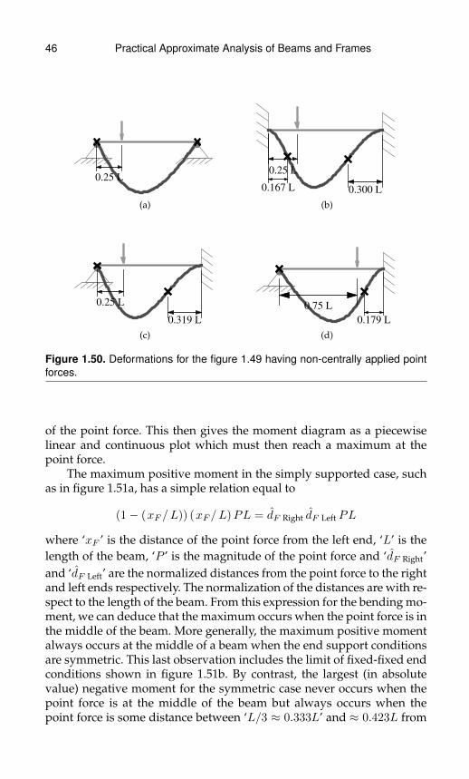
46 Practical Approximate Analysis of Beams and Frames
0.25 L
(a)
0.167 L 0.300 L
0.25 L
(b)
0.319 L
0.25 L
(c)
0.179 L
0.75 L
(d)
Figure 1.50. Deformations for the figure 1.49 having non-centrally applied pointforces.
of the point force. This then gives the moment diagram as a piecewiselinear and continuous plot which must then reach a maximum at thepoint force.
The maximum positive moment in the simply supported case, suchas in figure 1.51a, has a simple relation equal to
(1− (xF /L)) (xF /L)PL = dF Right dF Left PL
where ‘xF ’ is the distance of the point force from the left end, ‘L’ is thelength of the beam, ‘P ’ is the magnitude of the point force and ‘dF Right’and ‘dF Left’ are the normalized distances from the point force to the rightand left ends respectively. The normalization of the distances are with re-spect to the length of the beam. From this expression for the bending mo-ment, we can deduce that the maximum occurs when the point force is inthe middle of the beam. More generally, the maximum positive momentalways occurs at the middle of a beam when the end support conditionsare symmetric. This last observation includes the limit of fixed-fixed endconditions shown in figure 1.51b. By contrast, the largest (in absolutevalue) negative moment for the symmetric case never occurs when thepoint force is at the middle of the beam but always occurs when thepoint force is some distance between ‘L/3 ≈ 0.333L’ and ≈ 0.423L from

Practical Approximate Analysis of Beams and Frames 47
0
0.750PL
4
0
0.25 L
(a)
0.563PL
4
0.281PL
4
0.188PL
40.25 L
(b)
0
0.633PL
4
0.469PL
40.25 L
(c)
0
0.258PL
4
0.656PL
4
0.75 L
(d)
Figure 1.51. Moment diagrams for the figure 1.49 having non-centrally appliedpoint forces.
an end. These limits occur as the stiffness factor goes from the limit at in-finity (ie. fixed-fixed) to the limit at close to zero respectively. We say al-most hinged-hinged because the hinged-hinged case has zero momentsat each end.
The hinged-fixed cases in figure 1.49c and d have non-symmetricend conditions with xF = 0.25L and xF = 0.75L respectively. Due to thenon-symmetry of end conditions, their moment diagrams shown in fig-ures 1.51c and 1.51d are not mirror images of each other. For the hinged-fixed case, the maximum positive moment over all values of ‘xF ’ (ie. lo-cation of the point force) occurs when the point force is at a distance of≈ 0.366L from the hinged-end. We note that maximum positive momentwhen the point force is at 0.25L from the hinge is larger than when thepoint force is at the middle but smaller than when it is at 0.75L. Thelargest value that the maximum positive moment can have in the hinge-fixed case is when the point force is at ≈ 0.366L from the hinged endand has a value of ≈ 0.696PL/4 . By comparison, the negative momentat the fixed end in both figures 1.51c and 1.51d is smaller (in absolute

48 Practical Approximate Analysis of Beams and Frames
value) than the corresponding one when the point force is at the middle.The largest value that the negative moment can have in the hinge-fixedcase is when the point force is at ≈ 0.577L from the hinged end andhas a value of ≈ 0.770PL/4. This result is to be contrasted with the uni-form loading case as follows. If we consider the total load on a uniformlyloaded beam to be P = qL then for the hinged-spring case, the largestpositive moments are≈ 0.281PL/4 and≈ 0.5PL/4 respectively. The sig-nificantly larger values of ≈ 0.696PL/4 and ≈ 0.770PL/4 for the pointforce in both cases respectively is due to concentrating the load at a moreinfluential point in the beam or, equivalently, due to the added flexibilityin choosing the location of the point force.
Having considered some special cases, we now consider the generalcase shown in figure 1.52. A representative sketch of the deformed shapeand the bending moment diagram are shown in figures 1.52b and c. Asin the uniformly loaded case, in order to sketch the deformed shape, weneed to i) identify the approximate location of the inflection points andmark those by an ‘×,’ ii) roughly indicate the relative rotations of theleft versus the right end and iii) roughly indicate the right location ofthe maximum deflection. Of these three requirements, only the inflec-tion points need to be numerically indicated since their location will bethe basis for calculating the approximate values of the bending momentdiagram. We now discuss each of the three requirements separately.
PkL ´ 4
EI
L
kR ´ 4
EI
L
xF
(a)
kL ´ 4
EI
L
kR ´ 4
EI
L
xI Left xI Right
xF
(b)
MLeft
Min max
Mright
kL ´ 4
EI
L
kR ´ 4
EI
L
xF
(c)
Figure 1.52. General point force on a beam attached to passive structures onboth sides.
First we consider the locations of the inflection points. In general,there are two inflection points in a point force loaded beam that is at-tached to passive structures on both ends. These inflection points occurone on each side of the point force. The distance of an inflection pointfrom its nearest end increases as the stiffness factor of that end increasesand decreases as the point force approaches that end. For example, ifkR = 0 and the point force is at the center (ie. xF = 0.5L) then theleft inflection point is at x = 0 when kL = 0 (ie. a hinge at the leftend) and increases monotonically with ‘kL’ to reach a value of 0.273L

Practical Approximate Analysis of Beams and Frames 49
when kL → ∞. By considering the general case shown in figure 1.52a,we find that for any beam attached to passive structures on both endsand as the point force moves across the beam, the distance of an inflec-tion point to its nearest end may not exceed one third the length of thebeam (ie. ≈ 0.333L). This limit case occurs for the hinged-fixed or fixed-hinged case when the point force approaches the hinged end. In termsof lower limit, the distance of an inflection point to its nearest end maybe zero when the nearest end is a hinge. These two limits may be sum-marized by saying that the location of inflection points must always beoutside the middle third of the beam.
The location of an inflection point divided by the length of the beam(ie. normalized location) depends only on the spring stiffness factors ‘kL’and ‘kR’ and on the location of the point force (see figure 1.53). To getsome insight, we draw contour plots of the location of the left inflectionpoint versus the stiffness factors for various values of the coordinate ‘xF ’(origin at left end) of the point force (see figures 1.54). We notice that thelocation of an inflection point is rather insensitive to the stiffness factoron the right (ie. ‘kR’). Therefore, we consider obtaining a simple expres-sion for the location of the inflection points as a function of the stiff-ness factor near the end that it occurs multiplied by a function that onlydepends on the location of the point force ‘xF .’ This reduces the depen-dence of the location of an inflection point from three to two parametersat the expense of using an approximate expression. This approximateexpression will be presented and discussed next.
Mleft
Min max
Mright
kL ´ 4
EI
L
kR ´ 4
EI
L
xF
(a)
0
PL
4
0
xF
(b)
MleftMright
MleftMright
(c)
Figure 1.53. Superposition of moment diagrams for a beam with a point force.
Relatively simple expressions for the approximate locations of theinflection points for the beam shown in figure 1.52b are as follows:
xI Left/L ≈3kL
2 + 4kL× xF
1 + xF(1.6a)
1− xI Right/L ≈3kR
2 + 4kR× (1− xF )
1 + (1− xF )(1.6b)

50 Practical Approximate Analysis of Beams and Frames
0.01
0.02
0.03
0.04
0.05
0.06
0.07
0.08
0.09
0.1
0.11
0.12
0.13
0 1 2 3 4
0
1
2
3
4
kL
kR
xI left
xF = 0.2L
0.01
0.02
0.03
0.04
0.05
0.06
0.07
0.08
0.09
0.1
0.11
0.12
0.13
0.14
0.15
0.16
0.17
0.18
0.19
0.2
0.21
0 1 2 3 4
0
1
2
3
4
kL
kR
xI left
xF = 0.4L
0.01
0.02
0.03
0.04
0.05
0.06
0.07
0.08
0.09
0.1
0.11
0.12
0.13
0.14
0.15
0.16
0.17
0.18
0.19
0.2
0.21
0.22
0.23
0.24
0.25
0.26
0 1 2 3 4
0
1
2
3
4
kL
kR
xI left
xF = 0.6L
0.01
0.02
0.03
0.04
0.05
0.06
0.07
0.08
0.09
0.1
0.11
0.12
0.13
0.14
0.15
0.16
0.17
0.18
0.19
0.2
0.21
0.22
0.23
0.24
0.25
0.26
0.27
0.28
0 1 2 3 4
0
1
2
3
4
kL
kR
xI left
xF = 0.8L
Figure 1.54. Contour plot of the location of the inflection point versus end stiff-nesses for various locations of the point force.
where:
xI Left, xI Right, kL, kR and xF are illustrated in figures 1.52a and b.
L is the length of the beam
xF = xF /L , which is the normalized coordinate of the point force
P is the magnitude of the point force

Practical Approximate Analysis of Beams and Frames 51
0.5 1. 1.5 2. 2.5 3. 3.5 4.kL
-2.5
-2.
-1.5
-1.
-0.5
0
0.5
1.
1.5
2.
2.5
3.
DxIL�L%
Inflection point: Exact vs approximate
kR = 80, 0.25, 0.5, 1, 2, 4, ¥<
xF = 80.1, 0.2, 0.3, 0.4, 0.5, 0.6, 0.7, 0.8, 0.9<
Figure 1.55. Comparsion of inflection point location between exact and approxi-mate.
The results of the approximate expression 1.6a for the location ofthe left inflection point may be compared with the exact one and this isshown in figure 1.55. In that figure, each possible pairs of values of kRand xF where kR is selected from the first list and xF is selected fromthe second list generate one curve. All these curves lie between −2.5%and 3.5%. If we do an optimization to determine the maximum possibledifference between the approximate and the exact value for all valuesof stiffness factors and for all locations of the point force, we get thatthe maximum error is between about −3.0% and 4.1% and occur for thecases of fixed-hinged with the location of the point force at xF = 0.302and of fixed-fixed with the location of the point force xF → 1. Note thatthis is a percentage error which is relative to the length of the beam whilethe relative error relative to the location would be higher because we aredealing with small numbers. For the purposes of sketching and obtain-ing the bending moment diagram, it is the error relative to the lengththat is relevant. For example, when we are indicating the location of theinflection point on a sketch of the beam, the visual perception will be rel-ative to the length of the beam. In that regards,±4% would be barely dis-cernible. Moreover, in a manual sketch small features will be perceived
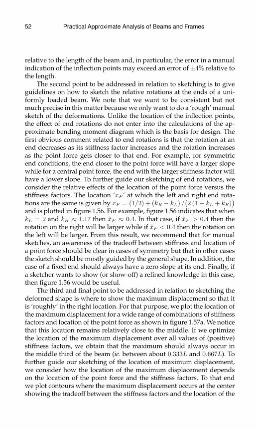
52 Practical Approximate Analysis of Beams and Frames
relative to the length of the beam and, in particular, the error in a manualindication of the inflection points may exceed an error of ±4% relative tothe length.
The second point to be addressed in relation to sketching is to giveguidelines on how to sketch the relative rotations at the ends of a uni-formly loaded beam. We note that we want to be consistent but notmuch precise in this matter because we only want to do a ‘rough’ manualsketch of the deformations. Unlike the location of the inflection points,the effect of end rotations do not enter into the calculations of the ap-proximate bending moment diagram which is the basis for design. Thefirst obvious comment related to end rotations is that the rotation at anend decreases as its stiffness factor increases and the rotation increasesas the point force gets closer to that end. For example, for symmetricend conditions, the end closer to the point force will have a larger slopewhile for a central point force, the end with the larger stiffness factor willhave a lower slope. To further guide our sketching of end rotations, weconsider the relative effects of the location of the point force versus thestiffness factors. The location ‘xF ’ at which the left and right end rota-tions are the same is given by xF = (1/2) + (kR − kL) /
(2 (1 + kL + kR)
)and is plotted in figure 1.56. For example, figure 1.56 indicates that whenkL = 2 and kR ≈ 1.17 then xF ≈ 0.4. In that case, if xF > 0.4 then therotation on the right will be larger while if xF < 0.4 then the rotation onthe left will be larger. From this result, we recommend that for manualsketches, an awareness of the tradeoff between stiffness and location ofa point force should be clear in cases of symmetry but that in other casesthe sketch should be mostly guided by the general shape. In addition, thecase of a fixed end should always have a zero slope at its end. Finally, ifa sketcher wants to show (or show-off) a refined knowledge in this case,then figure 1.56 would be useful.
The third and final point to be addressed in relation to sketching thedeformed shape is where to show the maximum displacement so that itis ‘roughly’ in the right location. For that purpose, we plot the location ofthe maximum displacement for a wide range of combinations of stiffnessfactors and location of the point force as shown in figure 1.57a. We noticethat this location remains relatively close to the middle. If we optimizethe location of the maximum displacement over all values of (positive)stiffness factors, we obtain that the maximum should always occur inthe middle third of the beam (ie. between about 0.333L and 0.667L). Tofurther guide our sketching of the location of maximum displacement,we consider how the location of the maximum displacement dependson the location of the point force and the stiffness factors. To that endwe plot contours where the maximum displacement occurs at the centershowing the tradeoff between the stiffness factors and the location of the
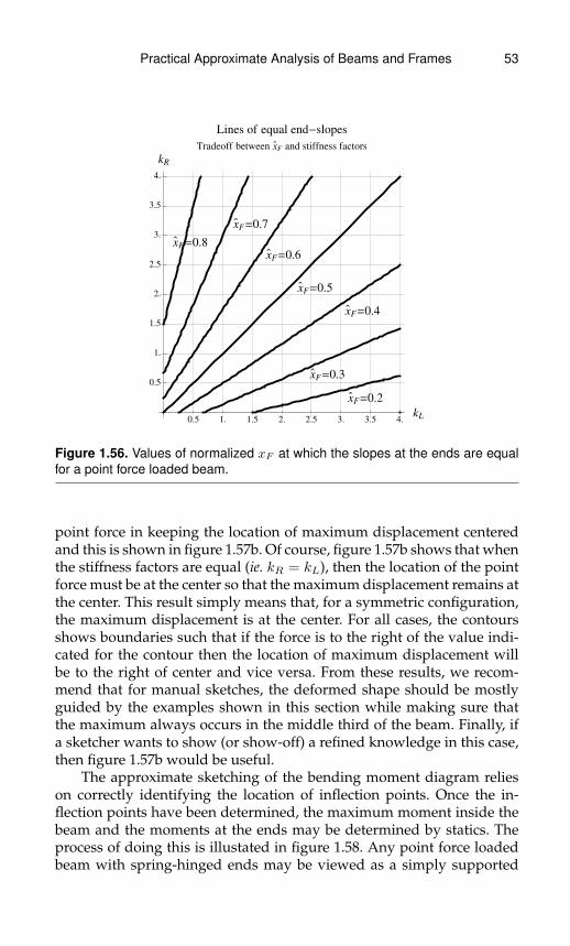
Practical Approximate Analysis of Beams and Frames 53
x`
F=0.2
x`
F=0.3
x`
F=0.4
x`
F=0.5
x`
F=0.6
x`
F=0.7
x`
F=0.8
0.5 1. 1.5 2. 2.5 3. 3.5 4.kL
0.5
1.
1.5
2.
2.5
3.
3.5
4.
kR
Lines of equal end-slopes
Tradeoff between x`
F and stiffness factors
Figure 1.56. Values of normalized xF at which the slopes at the ends are equalfor a point force loaded beam.
point force in keeping the location of maximum displacement centeredand this is shown in figure 1.57b. Of course, figure 1.57b shows that whenthe stiffness factors are equal (ie. kR = kL), then the location of the pointforce must be at the center so that the maximum displacement remains atthe center. This result simply means that, for a symmetric configuration,the maximum displacement is at the center. For all cases, the contoursshows boundaries such that if the force is to the right of the value indi-cated for the contour then the location of maximum displacement willbe to the right of center and vice versa. From these results, we recom-mend that for manual sketches, the deformed shape should be mostlyguided by the examples shown in this section while making sure thatthe maximum always occurs in the middle third of the beam. Finally, ifa sketcher wants to show (or show-off) a refined knowledge in this case,then figure 1.57b would be useful.
The approximate sketching of the bending moment diagram relieson correctly identifying the location of inflection points. Once the in-flection points have been determined, the maximum moment inside thebeam and the moments at the ends may be determined by statics. Theprocess of doing this is illustated in figure 1.58. Any point force loadedbeam with spring-hinged ends may be viewed as a simply supported
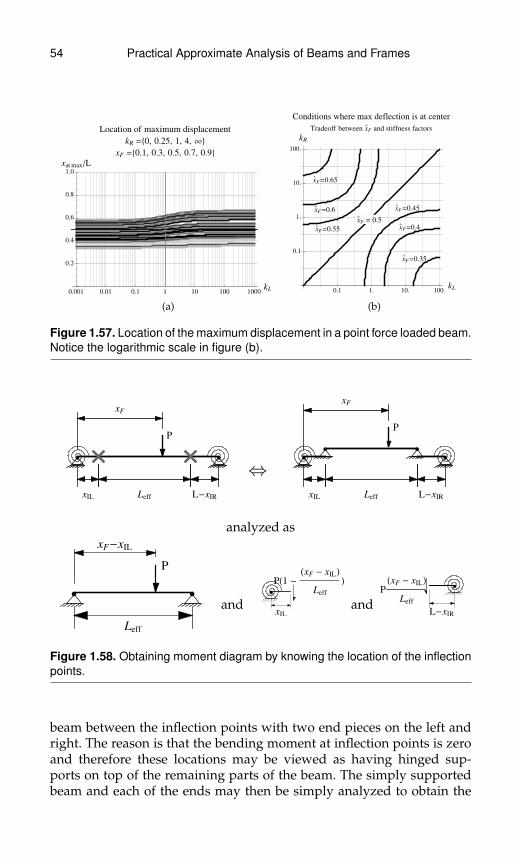
54 Practical Approximate Analysis of Beams and Frames
0.001 0.01 0.1 1 10 100 1000kL
0.2
0.4
0.6
0.8
1.0
xat max�L
Location of maximum displacement
kR =80, 0.25, 1, 4, ¥<
xF =80.1, 0.3, 0.5, 0.7, 0.9<
(a)
x`
F=0.35
x`
F=0.4
x`
F=0.45
x`
F=0.55
x`
F=0.6
x`
F=0.65
x`
F = 0.5
0.1 1. 10. 100.kL
0.1
1.
10.
100.
kR
Conditions where max deflection is at center
Tradeoff between x`
F and stiffness factors
(b)
Figure 1.57. Location of the maximum displacement in a point force loaded beam.Notice the logarithmic scale in figure (b).
P
xF
xIL Leff L-xIR
⇔
P
xF
xIL Leff L-xIR
analyzed as
P
xF-xIL
Leff
andxIL
PH1 -HxF - xILL
Leff
L
andL-xIR
P
HxF - xILL
Leff
Figure 1.58. Obtaining moment diagram by knowing the location of the inflectionpoints.
beam between the inflection points with two end pieces on the left andright. The reason is that the bending moment at inflection points is zeroand therefore these locations may be viewed as having hinged sup-ports on top of the remaining parts of the beam. The simply supportedbeam and each of the ends may then be simply analyzed to obtain the

Practical Approximate Analysis of Beams and Frames 55
maximum internal bending moment and the end moments while know-ing that the maximum positive moment occurs at the location of thepoint force. Referring to the notation shown in figure 1.58, the expres-sions for the maximum positive moment and the end moments are thengiven by:
Min max =P (xF − xIL)
(Leff − (xF − xIL)
)Leff
=P (xF − xIL) (xIR − xF )
Leff= dF eff right dF eff left PLeff (1.7a)
Mleft = −P (xIR − xF )xIL
Leff= − dF eff right PxIL (1.7b)
Mright = −P (xF − xIL) (L− xIR)
Leff= −dF eff left P (L− xIR) (1.7c)
where Min max, Mleft and Mright are the bending moments shown infigure 1.53
P is the magnitude of the point force
L is the length of the beam
Leff is the effective length of the beam which is illustrated in figure 1.58
xIL, xIR are the left and right coordinates of the inflection points
xF is the coordinate of the point force
dF eff right = xIR − xF is the distance from the point force to the rightinflection point
dF eff left = xF − xIL is the distance from the point force to the left in-flection point
dF eff right = dF eff right/Leff and dF eff left = dF eff left/Leff
Finally, using these critical values of the bending moment, we canconstruct the bending moment diagram. This diagram must be twostraight line segments of different slopes meeting at the location of thepoint force as in figure 1.52c. The reason is that the second derivative ofthe bending moment which equals the distributed load is zero since thereis no distributed load to the left or to the right of the point force. This sec-ond derivative is, from elementary mechanics, equal to the bending mo-ment. Also, at the point force, the bending moment must be continuous
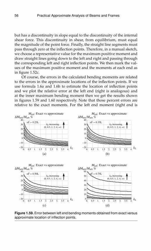
56 Practical Approximate Analysis of Beams and Frames
but has a discontinuity in slope equal to the discontinuity of the internalshear force. This discontinuity in shear, from equilibrium, must equalthe magnitude of the point force. Finally, the straight line segments mustpass through zero at the inflection points. Therefore, in a manual sketch,we choose a representative value for the maximum positive moment anddraw straight lines going down to the left and right and passing throughthe corresponding left and right inflection points. We then mark the val-ues of the maximum positive moment and the moments at each end asin figure 1.52c.
Of course, the errors in the calculated bending moments are relatedto the errors in the approximate locations of the inflection points. If weuse formula 1.6a and 1.6b to estimate the location of inflection pointsand we plot the relative error at the left end (right is analogous) andat the inner maximum bending moment then we get the results shownin figures 1.59 and 1.60 respectively. Note that those percent errors arerelative to the exact moments. For the left end moment (right end is
0. 0.5 1. 1.5 2. 2.5 3. 3.5 4.kL
-20
-10
0
10
20
30
40
DMleft�Mleft %
Mleft: Exact vs approximate
kR increasing
80, 0.5, 1, 2, 4,¥<
xF = 0.25L
(a)
0. 0.5 1. 1.5 2. 2.5 3. 3.5 4.kL
-20
-10
0
10
20
30
40
DMleft�Mleft %
Mleft: Exact vs approximate
kR increasing
80, 0.5, 1, 2, 4,¥<
xF = 0.35L
(b)
0. 0.5 1. 1.5 2. 2.5 3. 3.5 4.kL
-20
-10
0
10
20
30
40
DMleft�Mleft %
Mleft: Exact vs approximate
kR increasing
80, 0.5, 1, 2, 4,¥<
xF = 0.50L
(c)
0. 0.5 1. 1.5 2. 2.5 3. 3.5 4.kL
0
10
20
30
40
50
60
DMleft�Mleft %
Mleft: Exact vs approximate
kR increasing
80, 0.5, 1, 2, 4,¥<
xF = 0.75L
(d)
Figure 1.59. Error between left end bending moments obtained from exact versusapproximate location of inflection points.

Practical Approximate Analysis of Beams and Frames 57
0. 0.5 1. 1.5 2. 2.5 3. 3.5 4.kL
-5
0
5
10
15
20
25
DMin max�Min max %
Min max: Exact vs approximate
kR increasing
80, 0.5, 1, 2, 4,¥<
xF = 0.25L
(a)
0. 0.5 1. 1.5 2. 2.5 3. 3.5 4.kL
-5
0
5
10
15
20
25
DMin max�Min max %
Min max: Exact vs approximate
kR increasing
80, 0.5, 1, 2, 4,¥<
xF = 0.35L
(b)
0. 0.5 1. 1.5 2. 2.5 3. 3.5 4.kL
-5
0
5
10
15
20
25
DMin max�Min max %
Min max: Exact vs approximate
kR increasing
80, 0.5, 1, 2, 4,¥<
xF = 0.50L
(c)
0. 0.5 1. 1.5 2. 2.5 3. 3.5 4.kL
0
10
20
30
40
DMin max�Min max %
Min max: Exact vs approximate
kR increasing
80, 0.5, 1, 2, 4,¥<
xF = 0.75L
(d)
Figure 1.60. Error between maximum positive bending moments obtained fromexact versus approximate location of inflection points.
equivalent), we can obtain bounds on the relative error by optimizing therelative difference between the approximate and exact results. By doingthis, we find that if the approximately calculated end moment is greateror equal than 0.2PL/4, for any stiffness factors at the ends and any loca-tion of the point force then the relative error is between −23.5% whichoccurs when kL →∞, kR = 0 and xF ≈ 0.073L and 39.7% which occurswhen kL →∞, kR →∞ and xF ≈ 0.787L. These relative errors decreaseas the end moment gets larger or as the maximum stiffness factors at ei-ther end decreases. For example, if the stiffness factors at either end isless than 4 and the calculated approximate moment is greater or equalthan 0.1PL/4 (half the previous value) then the relative error is between−20.3% and 38.0%. Finally, the absolute error in the end moments is al-ways between −0.05PL/4 which occurs when kL → ∞, kR → ∞ andxF ≈ 0.785L and 0.12PL/4 which occurs when kL → ∞, kR = 0 andxF ≈ 0.284L.
For the inner maximum positive moment, by optimizing the dif-ference between the approximate and exact results, we find that if thepoint force remains within the middle half (ie. between 0.25L and 0.75L)
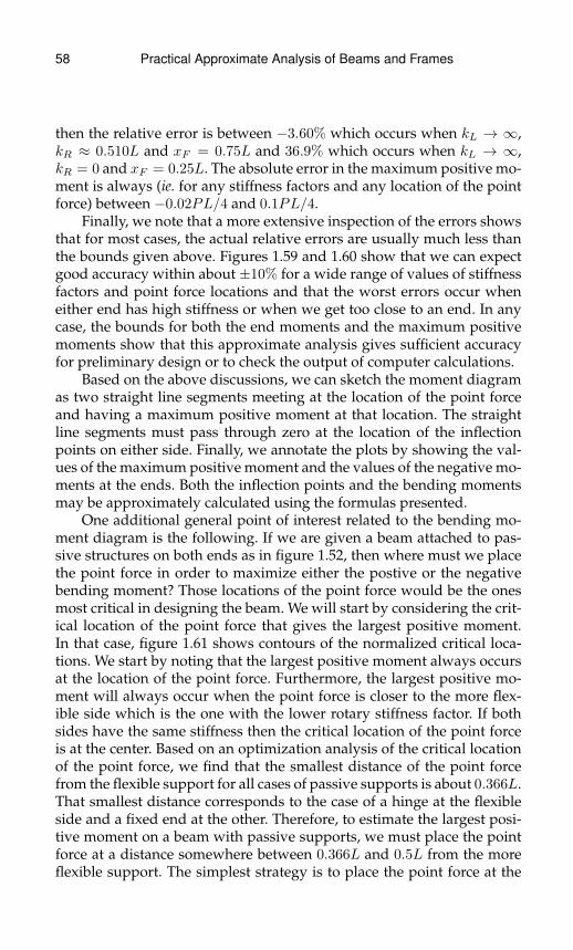
58 Practical Approximate Analysis of Beams and Frames
then the relative error is between −3.60% which occurs when kL → ∞,kR ≈ 0.510L and xF = 0.75L and 36.9% which occurs when kL → ∞,kR = 0 and xF = 0.25L. The absolute error in the maximum positive mo-ment is always (ie. for any stiffness factors and any location of the pointforce) between −0.02PL/4 and 0.1PL/4.
Finally, we note that a more extensive inspection of the errors showsthat for most cases, the actual relative errors are usually much less thanthe bounds given above. Figures 1.59 and 1.60 show that we can expectgood accuracy within about ±10% for a wide range of values of stiffnessfactors and point force locations and that the worst errors occur wheneither end has high stiffness or when we get too close to an end. In anycase, the bounds for both the end moments and the maximum positivemoments show that this approximate analysis gives sufficient accuracyfor preliminary design or to check the output of computer calculations.
Based on the above discussions, we can sketch the moment diagramas two straight line segments meeting at the location of the point forceand having a maximum positive moment at that location. The straightline segments must pass through zero at the location of the inflectionpoints on either side. Finally, we annotate the plots by showing the val-ues of the maximum positive moment and the values of the negative mo-ments at the ends. Both the inflection points and the bending momentsmay be approximately calculated using the formulas presented.
One additional general point of interest related to the bending mo-ment diagram is the following. If we are given a beam attached to pas-sive structures on both ends as in figure 1.52, then where must we placethe point force in order to maximize either the postive or the negativebending moment? Those locations of the point force would be the onesmost critical in designing the beam. We will start by considering the crit-ical location of the point force that gives the largest positive moment.In that case, figure 1.61 shows contours of the normalized critical loca-tions. We start by noting that the largest positive moment always occursat the location of the point force. Furthermore, the largest positive mo-ment will always occur when the point force is closer to the more flex-ible side which is the one with the lower rotary stiffness factor. If bothsides have the same stiffness then the critical location of the point forceis at the center. Based on an optimization analysis of the critical locationof the point force, we find that the smallest distance of the point forcefrom the flexible support for all cases of passive supports is about 0.366L.That smallest distance corresponds to the case of a hinge at the flexibleside and a fixed end at the other. Therefore, to estimate the largest posi-tive moment on a beam with passive supports, we must place the pointforce at a distance somewhere between 0.366L and 0.5L from the moreflexible support. The simplest strategy is to place the point force at the
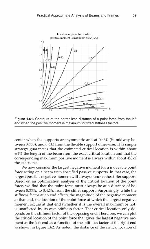
Practical Approximate Analysis of Beams and Frames 59
0.4
0.42
0.44
0.46
0.48
0.5
0.52
0.54 0.56
0.580.6
0.5 1. 1.5 2. 2.5 3. 3.5 4.kL
0.5
1.
1.5
2.
2.5
3.
3.5
4.
kR
Location of point force when
positive moment is maximum vs 8kL, kR<
Figure 1.61. Contours of the normalized distance of a point force from the leftend when the positive moment is maximum for fixed stiffness factors.
center when the supports are symmetric and at 0.43L (ie. midway be-tween 0.366L and 0.5L) from the flexible support otherwise. This simplestrategy guarantees that the estimated critical location is within about±7% the length of the beam from the exact critical location and that thecorresponding maximum positive moment is always within about 4% ofthe exact one.
We now consider the largest negative moment for a moveable pointforce acting on a beam with specified passive supports. In that case, thelargest possible negative moment will always occur at the stiffer support.Based on an optimization analysis of the critical location of the pointforce, we find that the point force must always be at a distance of be-tween 0.333L to 0.423L from the stiffer support. Surprisingly, while thestiffness factor at an end affects the magnitude of the negative momentat that end, the location of the point force at which the largest negativemoment occurs at that end (whether it is the overall maximum or not)is unaffected by its own stiffness factor. That critical location only de-pends on the stiffness factor of the opposing end. Therefore, we can plotthe critical location of the point force that gives the largest negative mo-ment at the left end as a function of the stiffness factor at the right endas shown in figure 1.62. As noted, the distance of the critical location of

60 Practical Approximate Analysis of Beams and Frames
0 0.5 1. 1.5 2. 2.5 3. 3.5 4.kR
0.34
0.36
0.38
0.4
0.42
xF at max�L
Location of point force when
left end moment is maximum vs kR
Figure 1.62. Location of a point force when the left end negative moment ismaximum as a function of the right-end stiffness factor.
the point force is always between 0.333L to 0.423L. Based on figure 1.62,we also note that the distance between the critical location of a pointforce and the stiffer end decreases as the stiffness factor of the far endincreases. The limits of 0.333L and 0.423L occur when the more flexi-ble support is either a fixed end or a hinge respectively. Based on thisdiscussion, we suggest that the simplest strategy to estimate the criticallocation of the point force is to always place the point force at a distanceof 0.38L (ie. about midway between 0.333L and 0.423L) from the stiffersupport. This simple strategy guarantees that the estimated critical loca-tion is always within about ±5% the length of the beam from the exactcritical location and that the corresponding maximum negative momentis always within about 1.5% of the exact one. Of course, when one of thesupports is a hinge, we could choose to place the point force at the exactcritical distance of about 0.423L from the other end.
To gain further insight with sketching the deformation and bend-ing moment diagrams, we present and discuss a range of results for thepoint force loaded beam. We begin by considering the case of symme-try where the passive structures at both ends provide about the sameresistance to deformations. This is indicated by having kL = kR = k intables 1.5 and 1.6. We start with the centrally loaded case of figure 1.5.Some interesting values of the stiffness factor ‘k’ include:
i) k = 0 (simply supported): This gives the largest possible positive mo-ment for a point force loaded beam attached to passive structures atboth ends.

Practical Approximate Analysis of Beams and Frames 61
Table 1.5. Point Force Loaded Beam: Symmetric Spring Resistance (xF = 0.5L).
Pk´4
EI
L
k´4
EI
L
0.50 L
k xInfl/L at left 1− xInf/L at right −Mleft/PL4−Mright/
PL4
Min max/PL4
0.000 0.000 0.000 0.000 0.000 1.0000.500 0.125 0.125 0.250 0.250 0.7500.750 0.150 0.150 0.300 0.300 0.7001.000 0.167 0.167 0.333 0.333 0.6671.500 0.188 0.188 0.375 0.375 0.6252.000 0.200 0.200 0.400 0.400 0.6003.000 0.214 0.214 0.429 0.429 0.5714.000 0.222 0.222 0.444 0.444 0.556∞ 0.250 0.250 0.500 0.500 0.500
Table 1.6. Point Force Loaded Beam: Symmetric Spring Resistance(xF = 0.25L ).
Pk´4
EI
L
k´4
EI
L
0.25 L
k xInfl/L at left 1− xInf/L at right −Mleft/PL4−Mright/
PL4
Min max/PL4
0.000 0.000 0.000 0.000 0.000 0.7500.500 0.076 0.155 0.234 0.141 0.5390.750 0.092 0.186 0.288 0.163 0.4941.000 0.103 0.206 0.325 0.175 0.4631.500 0.118 0.231 0.375 0.188 0.4222.000 0.127 0.245 0.407 0.193 0.3963.000 0.137 0.262 0.446 0.196 0.3664.000 0.144 0.271 0.470 0.197 0.348∞ 0.167 0.300 0.563 0.188 0.281
ii) k → ∞ (fixed-fixed): The negative moments at the ends are equal tothe positive one at the middle. If we minimize the maximum absolutevalue of bending moments in a central point force loaded beam for anybeam attached to passive supports and loaded with a point force in themiddle then we get this case. For a material whose yield in tension isthe same as in compression (eg. steel), this constitutes the end supportsthat would allow the largest central point force to be supported before
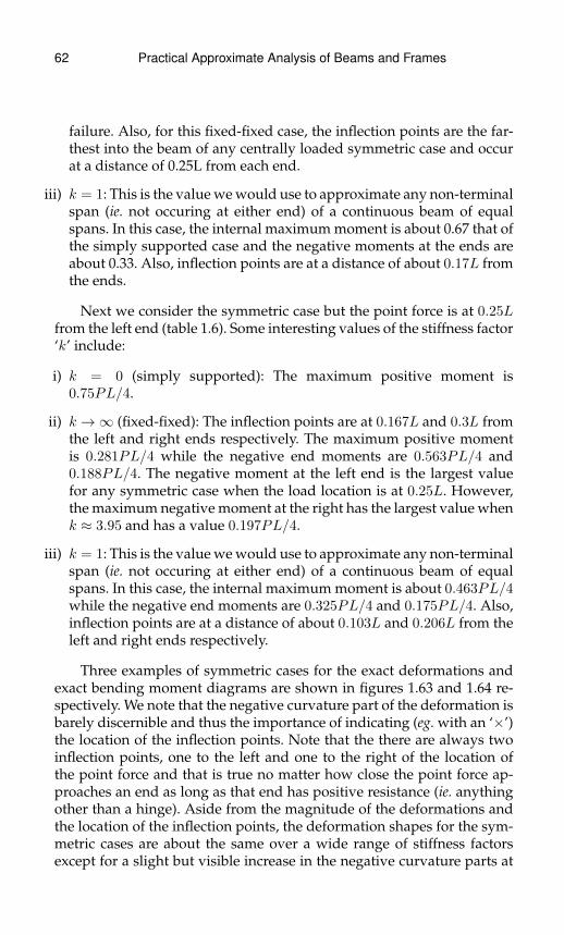
62 Practical Approximate Analysis of Beams and Frames
failure. Also, for this fixed-fixed case, the inflection points are the far-thest into the beam of any centrally loaded symmetric case and occurat a distance of 0.25L from each end.
iii) k = 1: This is the value we would use to approximate any non-terminalspan (ie. not occuring at either end) of a continuous beam of equalspans. In this case, the internal maximum moment is about 0.67 that ofthe simply supported case and the negative moments at the ends areabout 0.33. Also, inflection points are at a distance of about 0.17L fromthe ends.
Next we consider the symmetric case but the point force is at 0.25Lfrom the left end (table 1.6). Some interesting values of the stiffness factor‘k’ include:
i) k = 0 (simply supported): The maximum positive moment is0.75PL/4.
ii) k →∞ (fixed-fixed): The inflection points are at 0.167L and 0.3L fromthe left and right ends respectively. The maximum positive momentis 0.281PL/4 while the negative end moments are 0.563PL/4 and0.188PL/4. The negative moment at the left end is the largest valuefor any symmetric case when the load location is at 0.25L. However,the maximum negative moment at the right has the largest value whenk ≈ 3.95 and has a value 0.197PL/4.
iii) k = 1: This is the value we would use to approximate any non-terminalspan (ie. not occuring at either end) of a continuous beam of equalspans. In this case, the internal maximum moment is about 0.463PL/4while the negative end moments are 0.325PL/4 and 0.175PL/4. Also,inflection points are at a distance of about 0.103L and 0.206L from theleft and right ends respectively.
Three examples of symmetric cases for the exact deformations andexact bending moment diagrams are shown in figures 1.63 and 1.64 re-spectively. We note that the negative curvature part of the deformation isbarely discernible and thus the importance of indicating (eg. with an ‘×’)the location of the inflection points. Note that the there are always twoinflection points, one to the left and one to the right of the location ofthe point force and that is true no matter how close the point force ap-proaches an end as long as that end has positive resistance (ie. anythingother than a hinge). Aside from the magnitude of the deformations andthe location of the inflection points, the deformation shapes for the sym-metric cases are about the same over a wide range of stiffness factorsexcept for a slight but visible increase in the negative curvature parts at
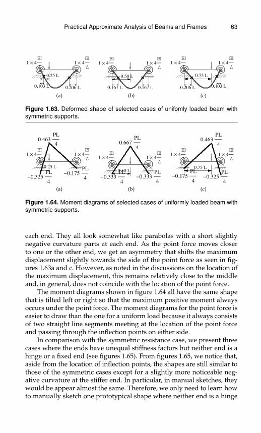
Practical Approximate Analysis of Beams and Frames 63
1 4EI
L1 4
EI
L
0.103 L 0.206 L
0.25 L
(a)
1 4EI
L1 4
EI
L
0.167 L 0.167 L
0.50 L
(b)
1 4EI
L1 4
EI
L
0.206 L 0.103 L
0.75 L
(c)
Figure 1.63. Deformed shape of selected cases of unifomly loaded beam withsymmetric supports.
0.325PL
4
0.463PL
4
0.175PL
4
1 4EI
L1 4
EI
L
0.25 L
(a)
0.333PL
4
0.667PL
4
0.333PL
4
1 4EI
L1 4
EI
L
0.50 L
(b)
0.175PL
4
0.463PL
4
0.325PL
4
1 4EI
L1 4
EI
L
0.75 L
(c)
Figure 1.64. Moment diagrams of selected cases of uniformly loaded beam withsymmetric supports.
each end. They all look somewhat like parabolas with a short slightlynegative curvature parts at each end. As the point force moves closerto one or the other end, we get an asymmetry that shifts the maximumdisplacement slightly towards the side of the point force as seen in fig-ures 1.63a and c. However, as noted in the discussions on the location ofthe maximum displacement, this remains relatively close to the middleand, in general, does not coincide with the location of the point force.
The moment diagrams shown in figure 1.64 all have the same shapethat is tilted left or right so that the maximum positive moment alwaysoccurs under the point force. The moment diagrams for the point force iseasier to draw than the one for a uniform load because it always consistsof two straight line segments meeting at the location of the point forceand passing through the inflection points on either side.
In comparison with the symmetric resistance case, we present threecases where the ends have unequal stiffness factors but neither end is ahinge or a fixed end (see figures 1.65). From figures 1.65, we notice that,aside from the location of inflection points, the shapes are still similar tothose of the symmetric cases except for a slightly more noticeable neg-ative curvature at the stiffer end. In particular, in manual sketches, theywould be appear almost the same. Therefore, we only need to learn howto manually sketch one prototypical shape where neither end is a hinge

64 Practical Approximate Analysis of Beams and Frames
1 4EI
L4 4
EI
L
0.098 L 0.277 L
0.25 L
(a)
1 4EI
L4 4
EI
L
0.159 L 0.230 L
0.50 L
(b)
1 4EI
L4 4
EI
L
0.200 L 0.148 L
0.75 L
(c)
Figure 1.65. Deformed shape of selected cases of point force loaded beam withnon-symmetric supports.
or a fixed end. The effect of the point force in the non-symmetric caseis similar to that of the symmetric case with figures 1.65a and c beingtypical.
The bending moment diagrams (figures 1.66) for the unsymmetriccase are similar to those of the symmetric ones. As with the symmetriccase, the maximum positive moment is always at the location of the pointforce. The procedure for manually sketching the moment diagrams of thenon-symmetric cases is identical to that of the symmetric ones.
0.298PL
4
0.459PL
4
0.269PL
4
1 4EI
L4 4
EI
L
0.25 L
(a)
0.282PL
4
0.603PL
4
0.513PL
4
1 4EI
L4 4
EI
L
0.50 L
(b)
0.125PL
4
0.344PL
4
0.500PL
4
1 4EI
L4 4
EI
L
0.75 L
(c)
Figure 1.66. Moment diagrams of selected cases of point force loaded beam withnon-symmetric supports.
The special case when one end is a hinge is next considered and thedeformations and bending moment diagrams are shown in figures 1.67and 1.68 respectively. Aside from having no inflection point on the sideof the free hinge, the shapes, if manually sketched would appear similarto the cases discussed above. For that reason, we will place a small ‘×’at the hinge in that case to distinguish it from the other cases. Note thatin figures 1.67, the location of the right inflection point only varies fromabout 0.11L to 0.21L as the point force moves from a distance of 0.25Lto 0.75L from the right support. As discussed previously, the inflectionpoint remains close to its nearest end and can never exceed a distance ofabout 0.333L from its nearest end even if the point force is almost at theopposite end (ie. in figures 1.67, this would be almost at the left end).

Practical Approximate Analysis of Beams and Frames 65
1 ´ 4
EI
L
0.211 L
0.25 L
(a)
1 ´ 4
EI
L
0.176 L
0.50 L
(b)
1 ´ 4
EI
L
0.111 L0.75 L
(c)
Figure 1.67. Deformed shape of selected cases of point force loaded beam withhinge-spring supports.
We show the bending moment diagrams of figures 1.67 infigures 1.68. These figures indicate that the special case of one end be-ing a hinge can only be distinguished from other cases by having a zeromoment at the hinged end. The rest of the procedure for sketching themoment diagram remains the same as seen in figures 1.68.
0
0.683PL
4
-0.268PL
4
1 ´ 4
EI
L
0.25 L
(a)
0
0.786PL
4
-0.429PL
4
1 ´ 4
EI
L
0.50 L
(b)
0
0.469PL
4
-0.375PL
4
1 ´ 4
EI
L
0.75 L
(c)
Figure 1.68. Moment diagrams of selected cases of point force loaded beam withhinge-spring supports.
The special case when one end is fixed is next considered and thedeformations and bending moment diagrams are shown in figures 1.69and 1.70 respectively. Aside from having zero slope and a more no-ticeable negative curvature near the fixed end, the shapes, if manuallysketched would appear similar to the cases discussed above. Note thatagain in figures 1.69, the location of either inflection point varies within arelatively narrow range as the point force moves from a distance of 0.25Lto 0.75L from the either support. As discussed previously, the inflectionpoint remains close to its nearest end and can never exceed a distance ofabout 0.333L from its nearest end even if the point force is almost at theopposite end.

66 Practical Approximate Analysis of Beams and Frames
1 ´ 4
EI
L
0.173 L 0.194 L
0.25 L
(a)
1 ´ 4
EI
L
0.263 L0.154 L
0.50 L
(b)
1 ´ 4
EI
L
0.313 L0.095 L
0.75 L
(c)
Figure 1.69. Deformed shape of selected cases of point force loaded beam withfixed-spring supports.
-0.609PL
4
0.270PL
4
-0.094PL
4
1 ´ 4
EI
L
0.25 L
(a)
-0.625PL
4
0.563PL
4
-0.250PL
4
1 ´ 4
EI
L
0.50 L
(b)
-0.328PL
4
0.457PL
4
-0.281PL
4
1 ´ 4
EI
L
0.75 L
(c)
Figure 1.70. Moment diagrams of selected cases of point force loaded beam withfixed-spring supports.
Concerning the bending moment diagrams of figures 1.69 shown infigures 1.70, the special case of one end being fixed is similar to the gen-eral unsymmetric cases discussed in figures. Therefore, these cases canbe sketched in a manner similar to the previous cases.
1.9 Example: Point ForceAs an example of applying the methods related to the point force, weconsider the structure shown in figure 1.71. We have only one memberloaded by a point force load of magnitude one and located at 1.75 unitsfrom point C with all the members having length 5 units and the samemoment of inertia ‘EI .’
As a first step, we decompose the structure into components(figure 1.72). We start with member CD (figure 1.72c). The stiffness fac-tor on the right is exactly 2 because the resistance on that side is pro-vided by two similar members that are fixed on the far end. The stiffnessfactor on the left is somewhere between 0.75 and 1 (exactly about 0.86),but, for simplicity, we take it to be equal to 1. Using formulas 1.6, wecalculate the approximate location of the inflection points, sketch the
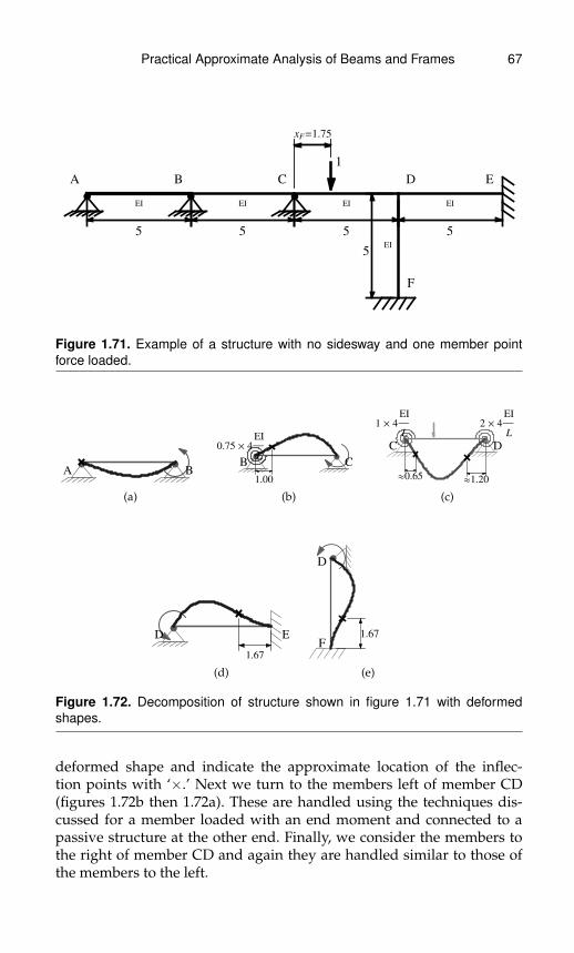
Practical Approximate Analysis of Beams and Frames 67
EI
5
EI
5
EI
5
EI
5
EI
5
1
A B C D E
F
xF=1.75
Figure 1.71. Example of a structure with no sidesway and one member pointforce loaded.
A B
(a)
0.75 ´ 4
EI
L
1.00
B C
(b)
1 ´ 4
EI
L
2 ´ 4
EI
L
»0.65»1.20
C D
(c)
1.67
D E
(d)
1.67
D
F
(e)
Figure 1.72. Decomposition of structure shown in figure 1.71 with deformedshapes.
deformed shape and indicate the approximate location of the inflec-tion points with ‘×.’ Next we turn to the members left of member CD(figures 1.72b then 1.72a). These are handled using the techniques dis-cussed for a member loaded with an end moment and connected to apassive structure at the other end. Finally, we consider the members tothe right of member CD and again they are handled similar to those ofthe members to the left.

68 Practical Approximate Analysis of Beams and Frames
EI
5
EI
5
EI
5
EI
5
EI
5
1
A B C D E
F
xF=1.75
1.00
0.601.17
1.67
1.67
Figure 1.73. Exact shape of the deformed structure of figure 1.71.
If we compare the approximate and exact locations (figure 1.73) ofinflection points we find good agreement. The largest error occurs at theinflection point in member CD near node C (0.9% of the beam length)and we attribute this error more to the approximate estimation of thestiffness factor at C where we used a round number of 1 instead of somenumber between 0.75 and 1 (eg. the mean 0.88). If we had used a stiffnessfactor at C of 0.88 then the error would have been about 0.3% of thebeam’s length.
Having obtained the approximate location of the inflection points,we then get the bending moments for the point force loaded beam usingformulas 1.7 and for the end-moment loaded beams using formulas 1.1.The results are shown in figure 1.74. We note the care in passing the lo-cation of zero bending moment through the inflection points in each ofthe members.
If we compare the approximate and exact values (figure 1.75) of max-imum and minimum bending moments, we again find good agreement.The largest error again occurs at node C. We note that the relative er-ror in the maximum positive and negative moments at the left and rightends which occur in member CD are only about 2.7%, −10.3% and 2.4%respectively.
Finally, we note that there is no need to sketch each of the membersseparately as shown in figures 1.72 and 1.74. We simply first sketch thedeformed shape while being aware of the process implied by figure 1.72and then do the same (on a separate sketch) for the bending moment dia-gram. With practice, this process becomes quick so that we only need oneor two minutes (with the aid of a calculator) to sketch an approximatedeformed shape and bending moment diagram for figure 1.71 which

Practical Approximate Analysis of Beams and Frames 69
»-0.11
A B
(a)
0.75 ´ 4
EI
L
0.200 L
»-0.43
»-0.11
B C
(b)
»-0.43
»-0.72
»-0.41
1 ´ 4
EI
L
2 ´ 4
EI
L
C D
(c)
0.333 L»-0.21
»-0.10
D E
(d)
0.333 L
»-0.21
»-0.10
D
F
(e)
Figure 1.74. Decomposition of structure shown in figure 1.71 with moment dia-grams.
EI
5
EI
5
EI
5
EI
5
EI
5
1
A B C D E
F
xF=1.75
0.100.10
-0.39
0.74
-0.42
-0.21
0.10
-0.21
0.10
Figure 1.75. Exact shape of the moment diagram of figure 1.71.
include approximate values for inflection points and bending momentsthat are indicated on the sketches. This level is relatively quickly attainedif the practioner becomes familiar with the results (including numericalvalues) shown in figures 1.63 to 1.70.

70 Practical Approximate Analysis of Beams and Frames
1.10 Comments and Exampleson Multiple Loads
If we load a structure so that there is only one loaded member or node,the magnitude of the response of a particular member in the structure de-creases rapidly as that member gets farther from the loaded member ornode (see figure 1.13 and related discussion). The influence of the load ishighest on the loaded member or node, then on the members directly at-tached to either end of the loaded member or node then on the membersdirectly attached to those members and so on. The reason for the rapiddecrease is primarily due to the carry over factor for moments which isalways less than half and usually around a third; as the member getsfarther from the loaded node or member, these carry over factors aremultiplied by each other and lead to a geometric type of decrease. Thedecrease may also be due to the distribution of an applied moment at anode over the attached members. This reduces the applied moment be-cause each connected member gets a fraction of the applied moment; ofcourse, this last effect is not present if we have a continuous beam sup-ported on rollers or hinges.
For linear analysis, we may superpose the response of single loads toobtain the effect of simultaneously applied multiple loads as illustratedin figure 1.77. Because of linear superposition and because of the rapidlydecreasing response when we load only a single member or node, the in-teraction of multiple loads of comparable magnitude is significant onlywhen the loaded members or nodes are separated by at most one mem-ber. In other cases, the deformations, bending moments or any responseof a member may be approximately evaluated as being only due to thenearest loaded member; members that may happen to be at equal dis-tances from two or more loads will generally have negligible values com-pared to the other members. Therefore, we will consider only two exam-ple cases, one with the loaded members separated by one member andone with the loaded members being adjacent.
Before proceeding with the examples in obtaining the bending mo-ment diagrams, we note the following basic observation in summing mo-ment diagrams:
• The sum of the plots of two straight line segments is a straight linesegment. Therefore, when we add two straight line segments, it is suf-ficient to sum the value at the ends of the segments.
• If we sum a piecewise straight line with a straight line segment, wewill obtain a piecewise straight line segment whose discontinuities areat the same locations as the original one. Therefore, it is sufficient to

Practical Approximate Analysis of Beams and Frames 71
sum values at each discontinuity point of the original straight line seg-ment.
• If we sum a parabolic segment with a straight line segment, we will ob-tain a parabolic segment. The location of the maximum of the resultingparabolic segment may be different than the original one. However,for the purpose of approximate analysis, we will assume that the lo-cation is about the same. Therefore, it is sufficient to sum the value atthe ends of the segments and at the location of the maximum of theoriginal parabolic segment.
If other cases are encountered then it is helpful to sketch the bendingmoment diagrams of each load case and estimate the location and valuesof the maxima and minima from those sketches.
We now consider an example of the case of two loaded membersseparated by one other member as shown in figure 1.76. There is a dis-tributed load whose net force is 1 × 5 = 5 units and a point force of4 units. To obtain the bending moment diagram, we will use superpo-sition as illustrated in figure 1.77. We will obtain the bending momentdiagrams for the distributed load and the point force load acting sepa-rately and add the separate values at each point to obtain their combinedbending moment diagram.
EI
3
EI
5
EI
5
EI
4EI
4EI
4
A B C D E
F G
q = 1P = 4
xF = 1.4
Figure 1.76. Multiple loads of comparable magnitude (total load) separated byone member.
First, we consider the structure loaded only with the distributed loadand, to approximately analyze it, we decompose the structure as shownin figure 1.78. We start with member BC (figure 1.78b). The stiffness fac-tor on the left and right are approximately (EI/3)/(EI/5) ≈ 1.67 and≈ (EI/4 + EI/5)/(EI/5) = 2.25 respectively. Using formulas 1.4, we

72 Practical Approximate Analysis of Beams and Frames
q P
=
q
+P
Figure 1.77. Superposition of multiple loads as the sum of separate single loads.
1.00
A B
(a)
1.67 ´ 4
EI
L
2.25 ´ 4
EI
L
»0.74 »0.83
B C
(b)
1.25 ´ 4
EI
L
1.19
C D
(c)
1.00 ´ 4
EI
L
0.89
D E
(d)
1.33
F
C
(e)
1.33
G
E
(f)
Figure 1.78. Decomposition of structure shown in figure 1.76 with deformedshapes when we only apply the distributed load.
calculate the approximate location of the inflection points, sketch thedeformed shape and indicate the approximate location of the inflectionpoints with ‘×.’ Next we turn to the members to the left (figure 1.78a) andright of member BC (figures 1.78c, d, e and f). These are all handled usingthe techniques discussed for a member loaded with an end moment andconnected to a passive structure at the other end. Note that the approx-imate location of all inflection points are indicated on the sketch of thedeformed structures. After we have obtained the approximate locationof the inflection points, we then get the bending moments for the uni-formly loaded beam using formulas 1.5 and for the end-moment loaded

Practical Approximate Analysis of Beams and Frames 73
beams using formulas 1.1. The corresponding exact results are given inone of the bending moment diagrams shown in the bottom left momentdiagram of figure 1.80. For comparison, if we consider the approximateresults for member BC then we get the following key values from left toright as −1.55, 1.47 and −1.76 versus −1.56, 1.48 and −1.74 as shown infigure 1.80 bottom left on member BC. This is excellent agreement for anapproximate analysis.
Next we consider the structure loaded only with the point forceload and, to approximately analyze it, we decompose the structure asshown in figure 1.79. We start with member DE (figure 1.79d). Thestiffness factor on the left and right are ≈ (EI/4)/(EI/5) = 0.8 and(EI/4)/(EI/4) = 1 respectively. Using formulas 1.6, we calculate theapproximate location of the inflection points, sketch the deformed shapeand indicate the approximate location of the inflection points with ‘×.’Next we turn to the members to the left (figure 1.79a, b, c and e) and rightof member DE (figures 1.78f). These are all handled using the techniquesdiscussed for a member loaded with an end moment and connected toa passive structure at the other end. Note that the approximate locationof all inflection points are indicated on the sketch of the deformed struc-tures. After we have obtained the approximate location of the inflectionpoints, we then get the bending moments for the uniformly loaded beamusing formulas 1.7 and for the end-moment loaded beams using formu-las 1.1. The corresponding exact results are given in one of the bending
1.00
A B
(a)
1.67 ´ 4
EI
L
1.28
B C
(b)
2.25 ´ 4
EI
L
1.36
C D
(c)
0.8 ´ 4
EI
L
1. ´ 4
EI
L
»0.48 »0.78
D E
(d)
1.33
F
C
(e)
1.33
G
E
(f)
Figure 1.79. Decomposition of structure shown in figure 1.76 with deformedshapes when we only apply the point force load.
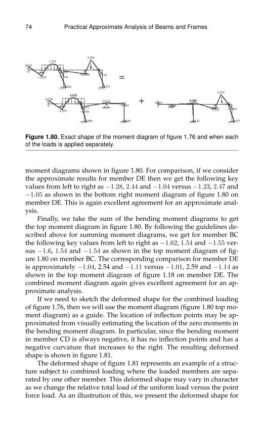
74 Practical Approximate Analysis of Beams and Frames
0.811
-1.623
1.541
-1.544
-0.262-1.014
2.591
-1.114
-0.641
1.282
-0.557
1.114
=
None
0.778
-1.557
1.479
-1.736
-0.717
0.213
-0.061
-0.509
1.018
-0.030
0.061 + 0.033
-0.066
0.1910.455
-1.227
2.474
-1.053
-0.132
0.264
-0.527
1.053
Figure 1.80. Exact shape of the moment diagram of figure 1.76 and when eachof the loads is applied separately.
moment diagrams shown in figure 1.80. For comparison, if we considerthe approximate results for member DE then we get the following keyvalues from left to right as −1.28, 2.44 and −1.04 versus −1.23, 2.47 and−1.05 as shown in the bottom right moment diagram of figure 1.80 onmember DE. This is again excellent agreement for an approximate anal-ysis.
Finally, we take the sum of the bending moment diagrams to getthe top moment diagram in figure 1.80. By following the guidelines de-scribed above for summing moment diagrams, we get for member BCthe following key values from left to right as −1.62, 1.54 and −1.55 ver-sus −1.6, 1.54 and −1.54 as shown in the top moment diagram of fig-ure 1.80 on member BC. The corresponding comparison for member DEis approximately −1.04, 2.54 and −1.11 versus −1.01, 2.59 and −1.14 asshown in the top moment diagram of figure 1.18 on member DE. Thecombined moment diagram again gives excellent agreement for an ap-proximate analysis.
If we need to sketch the deformed shape for the combined loadingof figure 1.76, then we will use the moment diagram (figure 1.80 top mo-ment diagram) as a guide. The location of inflection points may be ap-proximated from visually estimating the location of the zero moments inthe bending moment diagram. In particular, since the bending momentin member CD is always negative, it has no inflection points and has anegative curvature that increases to the right. The resulting deformedshape is shown in figure 1.81.
The deformed shape of figure 1.81 represents an example of a struc-ture subject to combined loading where the loaded members are sepa-rated by one other member. This deformed shape may vary in characteras we change the relative total load of the uniform load versus the pointforce load. As an illustrution of this, we present the deformed shape for
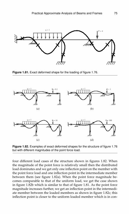
Practical Approximate Analysis of Beams and Frames 75
q = 1P = 4
Figure 1.81. Exact deformed shape for the loading of figure 1.76.
q = 1 P = 0.1
(a)
q = 1 P = 1
(b)
q = 1 P = 10
(c)
q = 1 P = 100
(d)
Figure 1.82. Examples of exact deformed shapes for the structure of figure 1.76but with different magnitudes of the point force load.
four different load cases of the structure shown in figures 1.82. Whenthe magnitude of the point force is relatively small then the distributedload dominates and we get only one inflection point on the member withthe point force load and one inflection point in the intermediate memberbetween them (see figure 1.82a). When the point force magnitude be-comes comparable to that of the uniform load, we get the case shownin figure 1.82b which is similar to that of figure 1.81. As the point forcemagnitude increases further, we get an inflection point in the intermedi-ate member between the loaded members as shown in figure 1.82c; thisinflection point is closer to the uniform loaded member which is in con-
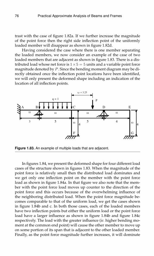
76 Practical Approximate Analysis of Beams and Frames
trast with the case of figure 1.82a. If we further increase the magnitudeof the point force then the right side inflection point of the uniformlyloaded member will disappear as shown in figure 1.82d.
Having considered the case where there is one member separatingthe loaded members, we now consider an example of the case of twoloaded members that are adjacent as shown in figure 1.83. There is a dis-tributed load whose net force is 1×5 = 5 units and a variable point forcemagnitude denoted by P . Since the bending moment diagram may be di-rectly obtained once the inflection point locations have been identified,we will only present the deformed shape including an indication of thelocation of all inflection points.
EI
3
EI
5
EI
5
EI
4EI
4EI
4
A B C D E
F G
q = 1P
xF = 3.25
Figure 1.83. An example of multiple loads that are adjacent.
In figures 1.84, we present the deformed shape for four different loadcases of the structure shown in figures 1.83. When the magnitude of thepoint force is relatively small then the distributed load dominates andwe get only one inflection point on the member with the point forceload as shown in figure 1.84a. In that figure we also note that the mem-ber with the point force load moves up counter to the direction of thepoint force and this occurs because of the overwhelming influence ofthe neighboring distributed load. When the point force magnitude be-comes comparable to that of the uniform load, we get the cases shownin figure 1.84b and c. In both those cases, each of the loaded membershave two inflection points but either the uniform load or the point forceload have a larger influence as shown in figure 1.84b and figure 1.84crespectively. The load with the greater influence (ie. higher bending mo-ment at the common end point) will cause the other member to move upon some portion of its span that is adjacent to the other loaded member.Finally, as the point force magnitude further increases, it will dominate
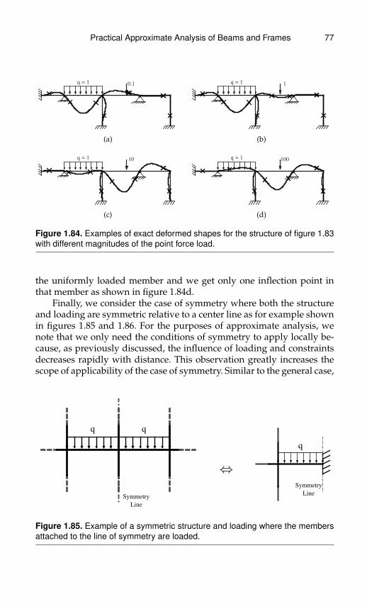
Practical Approximate Analysis of Beams and Frames 77
q = 1 0.1
(a)
q = 1 1
(b)
q = 1 10
(c)
q = 1 100
(d)
Figure 1.84. Examples of exact deformed shapes for the structure of figure 1.83with different magnitudes of the point force load.
the uniformly loaded member and we get only one inflection point inthat member as shown in figure 1.84d.
Finally, we consider the case of symmetry where both the structureand loading are symmetric relative to a center line as for example shownin figures 1.85 and 1.86. For the purposes of approximate analysis, wenote that we only need the conditions of symmetry to apply locally be-cause, as previously discussed, the influence of loading and constraintsdecreases rapidly with distance. This observation greatly increases thescope of applicability of the case of symmetry. Similar to the general case,
q q
Symmetry
Line
⇔
q
Symmetry
Line
Figure 1.85. Example of a symmetric structure and loading where the membersattached to the line of symmetry are loaded.
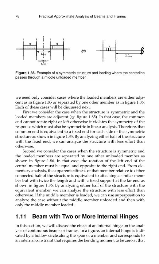
78 Practical Approximate Analysis of Beams and Frames
q q
Symmetry
Line
Lmid
⇔q
2 Lmid
Figure 1.86. Example of a symmetric structure and loading where the centerlinepasses through a middle unloaded member.
we need only consider cases where the loaded members are either adja-cent as in figure 1.85 or separated by one other member as in figure 1.86.Each of these cases will be discussed next.
First we consider the case when the structure is symmetric and theloaded members are adjacent (eg. figure 1.85). In that case, the commonend cannot rotate right or left otherwise it violates the symmetry of theresponse which must also be symmetric in linear analysis. Therefore, thatcommon end is equivalent to a fixed end for each side of the symmetricstructure as shown in figure 1.85. By analyzing either half of the structurewith the fixed end, we can analyze the structure with less effort thanotherwise.
Second we consider the cases when the structure is symmetric andthe loaded members are separated by one other unloaded member asshown in figure 1.86. In that case, the rotation of the left end of thecentral member must be equal and opposite to the right end. From ele-mentary analysis, the apparent stiffness of that member relative to eitherconnected half of the structure is equivalent to attaching a similar mem-ber but with twice the length and with a fixed support at the far end asshown in figure 1.86. By analyzing either half of the structure with theequivalent member, we can analyze the structure with less effort thanotherwise. If the middle member is loaded, we can use superposition toanalyze the case without the middle member unloaded and then withonly the middle member loaded.
1.11 Beam with Two or More Internal HingesIn this section, we will discuss the effect of an internal hinge on the anal-ysis of continuous beams or frames. In a figure, an internal hinge is indi-cated by a hollow circle along the span of a member and corresponds toan internal constraint that requires the bending moment to be zero at that

Practical Approximate Analysis of Beams and Frames 79
location. While it is admissible to apply a point force at an internal hingewe must be careful when specifying an applied point or concentratedmoment. When applying such a moment, we must specify whether thatmoment is actually applied on the member to the left or to the right ofthe internal hinge. In fact, it is admissible to apply two point moments,one to the left and one to the right of the internal hinge and this kind ofloading has an important application in the study of influence lines.
We start by considering the case of three or more internal hinges ina bending member. Such members are always statically unstable if weapply any load on their span irrespective of the end conditions or sup-ports. The reason is that a bending member must satisfy two boundaryconditions associated with the bending deformations at each end. Theseconditions may be of the support (eg. no rotation), of the loading type(eg. applied end moment) or of a combination of both. Two of thoseboundary conditions must directly or indirectly constrain the rigid bodymotion of the member. This then leaves only two ‘free’ equations to sat-isfy other constraints. With three or more internal hinges, we have moreconstraints than can be met by a bending member. Therefore, any mem-ber with three or more internal hinges may be removed from the struc-ture as being structurally irrelevant.
From the above, we deduce that we only need to consider the case ofone or two internal hinges. We start with the case of a bending memberwith two internal hinges and we wil divide the discussion into two parts:i) when the member is acting as part of a passive structure as shown infigure 1.87 and ii) when the member is attached on both ends to passivestructures while being loaded over its span. By considering these twocases, we can then use the methods developed previously to do an ap-proximate analysis for any structure containing one or more memberseach having two internal hinges.
To study the member having two internal hinges as part of a pas-sive structure, we consider it under the conditions shown in figure 1.87.The figure shows an applied rotation at one end and a rotary spring at
Θnear
Figure 1.87. A beam with two internal hinges considered as part of a passivestructure.
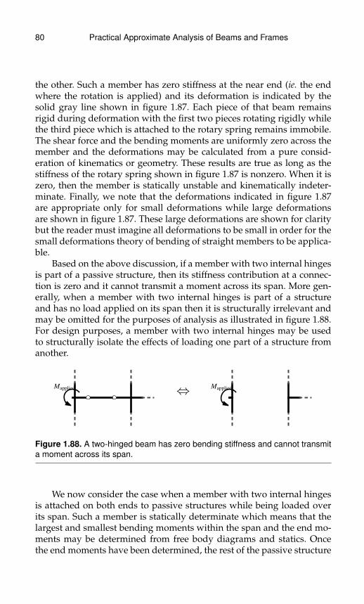
80 Practical Approximate Analysis of Beams and Frames
the other. Such a member has zero stiffness at the near end (ie. the endwhere the rotation is applied) and its deformation is indicated by thesolid gray line shown in figure 1.87. Each piece of that beam remainsrigid during deformation with the first two pieces rotating rigidly whilethe third piece which is attached to the rotary spring remains immobile.The shear force and the bending moments are uniformly zero across themember and the deformations may be calculated from a pure consid-eration of kinematics or geometry. These results are true as long as thestiffness of the rotary spring shown in figure 1.87 is nonzero. When it iszero, then the member is statically unstable and kinematically indeter-minate. Finally, we note that the deformations indicated in figure 1.87are appropriate only for small deformations while large deformationsare shown in figure 1.87. These large deformations are shown for claritybut the reader must imagine all deformations to be small in order for thesmall deformations theory of bending of straight members to be applica-ble.
Based on the above discussion, if a member with two internal hingesis part of a passive structure, then its stiffness contribution at a connec-tion is zero and it cannot transmit a moment across its span. More gen-erally, when a member with two internal hinges is part of a structureand has no load applied on its span then it is structurally irrelevant andmay be omitted for the purposes of analysis as illustrated in figure 1.88.For design purposes, a member with two internal hinges may be usedto structurally isolate the effects of loading one part of a structure fromanother.
Mapplied ⇔ Mapplied
Figure 1.88. A two-hinged beam has zero bending stiffness and cannot transmita moment across its span.
We now consider the case when a member with two internal hingesis attached on both ends to passive structures while being loaded overits span. Such a member is statically determinate which means that thelargest and smallest bending moments within the span and the end mo-ments may be determined from free body diagrams and statics. Oncethe end moments have been determined, the rest of the passive structure

Practical Approximate Analysis of Beams and Frames 81
may be approximately analyzed using the developed procedures. If ei-ther end of a beam with two internal hinges is attached to a hinge with norotary stiffness then the beam is statically unstable and thus structurallyirrelevant. Such a beam must be free of any loading and may again beomitted for the purposes of analysis.
The placement of internal hinges in a beam is usually by design butmay also be encountered in structural integrity assessments of partiallyfailed structures. If the internal hinges in a beam are to be introduced bydesign then it is natural to ask where should we place them. The answerdepends on the type of loading that is applied on the span. If we considerthe case of a uniform load, then the lowest bending moment in absolutevalue (ie. positive or negative) is obtained when the internal hinges areat(2±√
2)L/4 ≈ (0.146, 0.854)L and has a value of qL2
/16. This op-
timal placement of the internal hinges is independent of the stiffness ofthe passive structures attached to the ends of the beam because a beamwith two internal hinges is statically determinate. Of course, the passivestructures must provide non-zero stiffness at both ends to avoid load-ing a statically unstable beam. If the beam was without internal hingesthen this optimal location of internal hinges correspond to the location ofthe inflection points when the stiffness factors on the beam at both endsequals 1.5.
If we consider a pont force loading that may occur anywhere onthe span, then the lowest bending moment in absolute value in a beamwith two internal hinges is obtained when the internal hinges are at(1/4, 3/4)L and has a value of PL/8. This optimal placement of the in-ternal hinges is independent of the stiffness of the passive structures at-tached to the ends of the beam because a beam with two internal hingesis statically determinate. Again, the passive structures must provide non-zero stiffness at both ends to avoid loading a statically unstable beam. Ifthe beam was without internal hinges then this optimal location of inter-nal hinges correspond to the location of the inflection points when thepoint force is at the middle of the beam and the stiffness factors on thebeam at both ends are indefinitely large (ie. k →∞) which correspond tofixed supports.
If we want to avoid the worst placement of two internal hinges in abeam then the following results apply. For uniform loading or for pointforce loading, the worst conditions in terms of getting the largest possi-ble positive bending moment occurs when we place one internal hingeat the left end and the other at the right end so as to effectively producea simply supported beam. This produces a maximum positive bendingmoment of qL2
/8 and PL/4 for the uniform load and point force load
respectively. However, the worst conditions for the largest possible neg-ative bending moment or of the largest poosible absolute value of the

82 Practical Approximate Analysis of Beams and Frames
bending moment occurs when we place both internal hinges infinites-imally or very close to each other and infinitesimally or very close toeither end of the beam. This produces a maximum negative bendingmoment of qL2
/2 and PL for the uniform load and point force load
respectively. These values are four times larger than the correspond-ing ones for maximum positive moment and they correspond to thevalues obtained for a cantilever which is a member supported on onlyone side.
How did the two internal hinges produce an effect equivalent to acantilever? When two internal hinges occur in a beam, the part of thebeam in between the internal hinges acts like a link providing zero verti-cal stiffness and zero rotary stiffness to either of its attached ends. If wemake a very small link of this kind and place it near one end of the beam,then that end will be structurally isolated from the rest of the beam sinceit cannot affect the other side either through vertical or through rotaryresistance. The part of the beam from the internal hinges to the othersupport then effectively becomes a cantilever and we get the largest pos-sible bending moments for the loading cases considered. We note thatplacing two internal hinges very close to each other appears to be ge-ometrically similar to having one internal hinge. However, the effect oftwo very close internal hinges is structurally different than one inter-nal hinge. The reason is that we can transmit shear across one internalhinge but not across a link member formed between two internal hinges.Both the vertical and rotational isolation are needed to get the condi-tions of a cantiliver which produce the largest bending moment underthe considered types of loading. Of course, the distance between twointernal hinges cannot be infinitesimal but must be constrained by phys-ical and geometric considerations. However, the optimization result forthe largest negative moments provides a bound or limit which when ap-proached leads to severe bending moments on a loaded beam.
Having considered the general behavior of a loaded beam withtwo internal hinges attached to passive structures on each end, we willdiscuss how to sketch the deformed shape and the bending momentdiagram of such a member. Such knowledge is needed to sketch the de-formed shape and bending moment diagrams of a whole structure con-taining one or more members of this type.
We start by considering a beam with two internal hinges loaded bya uniform load and attached to passive structures on both ends. Exam-ples of such deformations for various locations of the internal hingesare shown in figure 1.89. The behavior of each piece of the beam fromone end to the nearest internal hinge is that of a uniformly loaded can-tilever but with flexible support. Such a cantilever will have an initialrotation at the support and a negative cuvature throughout its span. The

Practical Approximate Analysis of Beams and Frames 83
4 ´ 4
EI
L
4 ´ 4
EI
L
(a)
4 ´ 4
EI
L
4 ´ 4
EI
L
(b)
4 ´ 4
EI
L
4 ´ 4
EI
L
(c)
1 ´ 4
EI
L
1 ´ 4
EI
L
(d)
1 ´ 4
EI
L
(e)
0.5 ´ 4
EI
L
4 ´ 4
EI
L
(f)
Figure 1.89. Examples of the deformations of a beam with two internal hingesloaded by a uniform load and attached to passive structures on both ends.
tip deflection of such a cantilever(qL4(1 + k)/8kEI
)where ‘q’ is the dis-
tributed load, ‘E’ is Young’s modulus, ‘I’ is the moment of inertia, ‘L’is the length of the cantilever and ‘k’ is the rotary spring stiffness factorat the supported end. The important point to note is that the deflectionis proportional to the fourth power of the length of the beam so that ifthe length doubles, the deflection increases by a factor of 16. This obser-vation explains the relative deflections of the internal hinges shown infigures 1.89d, e and f where the relative deflection at the internal hingeschanges rapidly with the ratio of their respective lengths. Finally, themiddle portion of the beam deflects like a simply supported beam butwhose supports are subsequently moved to match the deflection of theinternal hinges. For the same length and under a uniform load, the max-imum deflection of a simply supported beam is 9.6 times less than thatof a cantilever of comparable length but with fixed support. That is whythe separation between the hinges must be relatively large compared toeither of the end pieces in order for the deflection of the middle portionto appear significant as demonstrated by the examples in figures 1.89b,c, d, e and f. When the length of the middle piece is less or equal to thelength of at least one end piece of the beam and when the stiffness factorat the support of that end piece is less or equal to 2, then its deforma-tion is relatively insignificant and the middle piece appears almost like astraight line as illustrated in figures 1.89d and e.
The bending moment diagrams of a loaded beam with two inter-nal hinges loaded by a uniform load and attached to passive structureson both ends is always a parabola passing through each of the internal
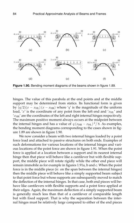
84 Practical Approximate Analysis of Beams and Frames
4 ´ 4
EI
L
4 ´ 4
EI
L
(a)
4 ´ 4
EI
L
4 ´ 4
EI
L
(b)
4 ´ 4
EI
L
4 ´ 4
EI
L
(c)
1 ´ 4
EI
L
1 ´ 4
EI
L
(d)
1 ´ 4
EI
L
(e)
0.5 ´ 4
EI
L
4 ´ 4
EI
L
(f)
Figure 1.90. Bending moment diagrams of the beams shown in figure 1.89.
hinges. The value of this parabola at the end points and at the middlesupport may be determined from statics. Its functional form is givenby (q/2)(x − xHL) (x− xHR) where ‘q’ is the magnitude of the uniformload, ‘x’ is the coordinate of any point from the left end and ‘xHL’ and‘xHR’ are the coordinates of the left and right internal hinges respectively.The maximum positive moment always occurs at the midpoint betweenthe internal hinges and has a value of q (xHR − xHL) 2
/8. As examples,
the bending moment diagrams corresponding to the cases shown in fig-ure 1.89 are shown in figure 1.90.
We now consider a beam with two internal hinges loaded by a pointforce load and attached to passive structures on both ends. Examples ofsuch deformations for various locations of the internal hinges and vari-ous locations of the point force are shown in figure 1.91. When the pointforce is applied at a location between a support and its nearest internalhinge then that piece will behave like a cantilever but with flexible sup-port, the middle piece will rotate rigidly while the other end piece willremain immobile as for example in figures 1.91a, b and c. When the pointforce is in the middle piece (ie. on the span between the internal hinges)then the middle piece will behave like a simply supported beam subjectto that point force but whose supports are subsequently moved to matchthe deflection of the internal hinges. In that case, both end pieces will be-have like cantilevers with flexible supports and a point force applied attheir edges. Again, the maximum deflection of a simply supported beamis generally much less than that of a cantilever of comparable lengthbut with fixed support. That is why the separation between the inter-nal hinges must be relatively large compared to either of the end pieces
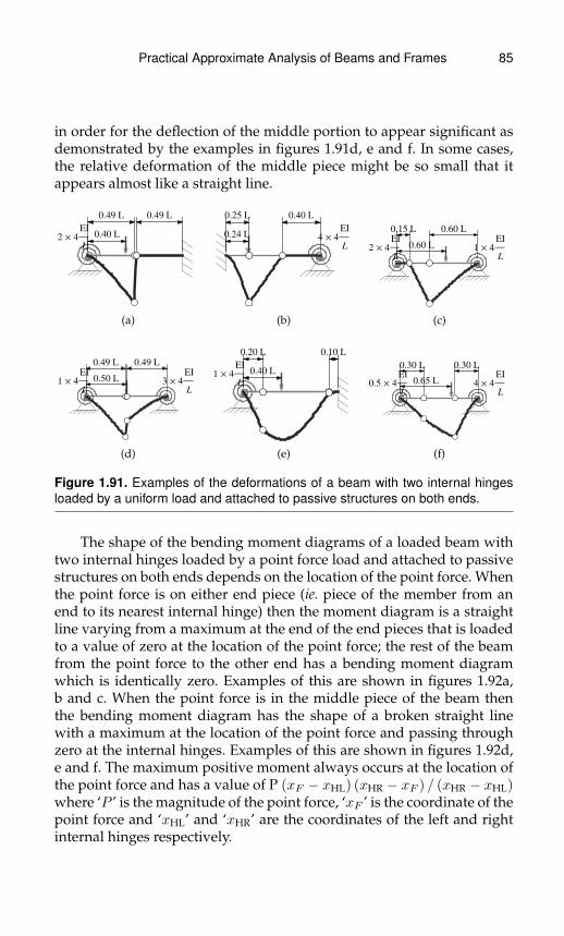
Practical Approximate Analysis of Beams and Frames 85
in order for the deflection of the middle portion to appear significant asdemonstrated by the examples in figures 1.91d, e and f. In some cases,the relative deformation of the middle piece might be so small that itappears almost like a straight line.
0.49 L 0.49 L
0.40 L2 ´ 4
EI
L
(a)
0.25 L 0.40 L
0.24 L 4 ´ 4
EI
L
(b)
0.15 L 0.60 L
0.60 L2 ´ 4
EI
L
1 ´ 4
EI
L
(c)
0.49 L 0.49 L
0.50 L1 ´ 4
EI
L
3 ´ 4
EI
L
(d)
0.20 L 0.10 L
0.40 L1 ´ 4
EI
L
(e)
0.30 L 0.30 L
0.65 L0.5 ´ 4
EI
L
4 ´ 4
EI
L
(f)
Figure 1.91. Examples of the deformations of a beam with two internal hingesloaded by a uniform load and attached to passive structures on both ends.
The shape of the bending moment diagrams of a loaded beam withtwo internal hinges loaded by a point force load and attached to passivestructures on both ends depends on the location of the point force. Whenthe point force is on either end piece (ie. piece of the member from anend to its nearest internal hinge) then the moment diagram is a straightline varying from a maximum at the end of the end pieces that is loadedto a value of zero at the location of the point force; the rest of the beamfrom the point force to the other end has a bending moment diagramwhich is identically zero. Examples of this are shown in figures 1.92a,b and c. When the point force is in the middle piece of the beam thenthe bending moment diagram has the shape of a broken straight linewith a maximum at the location of the point force and passing throughzero at the internal hinges. Examples of this are shown in figures 1.92d,e and f. The maximum positive moment always occurs at the location ofthe point force and has a value of P (xF − xHL) (xHR − xF ) / (xHR − xHL)where ‘P ’ is the magnitude of the point force, ‘xF ’ is the coordinate of thepoint force and ‘xHL’ and ‘xHR’ are the coordinates of the left and rightinternal hinges respectively.
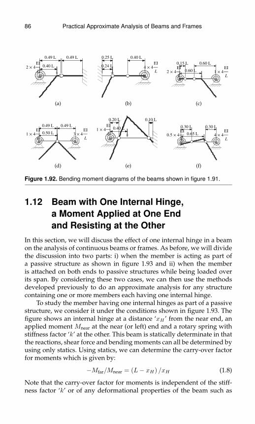
86 Practical Approximate Analysis of Beams and Frames
0.49 L 0.49 L
0.40 L2 ´ 4
EI
L
(a)
0.25 L 0.40 L
0.24 L 4 ´ 4
EI
L
(b)
0.15 L 0.60 L
0.60 L2 ´ 4
EI
L
1 ´ 4
EI
L
(c)
0.49 L 0.49 L
0.50 L1 ´ 4
EI
L
3 ´ 4
EI
L
(d)
0.20 L 0.10 L
0.40 L1 ´ 4
EI
L
(e)
0.30 L 0.30 L
0.65 L0.5 ´ 4
EI
L
4 ´ 4
EI
L
(f)
Figure 1.92. Bending moment diagrams of the beams shown in figure 1.91.
1.12 Beam with One Internal Hinge,a Moment Applied at One Endand Resisting at the Other
In this section, we will discuss the effect of one internal hinge in a beamon the analysis of continuous beams or frames. As before, we will dividethe discussion into two parts: i) when the member is acting as part ofa passive structure as shown in figure 1.93 and ii) when the memberis attached on both ends to passive structures while being loaded overits span. By considering these two cases, we can then use the methodsdeveloped previously to do an approximate analysis for any structurecontaining one or more members each having one internal hinge.
To study the member having one internal hinges as part of a passivestructure, we consider it under the conditions shown in figure 1.93. Thefigure shows an internal hinge at a distance ‘xH ’ from the near end, anapplied moment Mnear at the near (or left) end and a rotary spring withstiffness factor ‘k’ at the other. This beam is statically determinate in thatthe reactions, shear force and bending moments can all be determined byusing only statics. Using statics, we can determine the carry-over factorfor moments which is given by:
−Mfar/Mnear = (L− xH) /xH (1.8)
Note that the carry-over factor for moments is independent of the stiff-ness factor ‘k’ or of any deformational properties of the beam such as
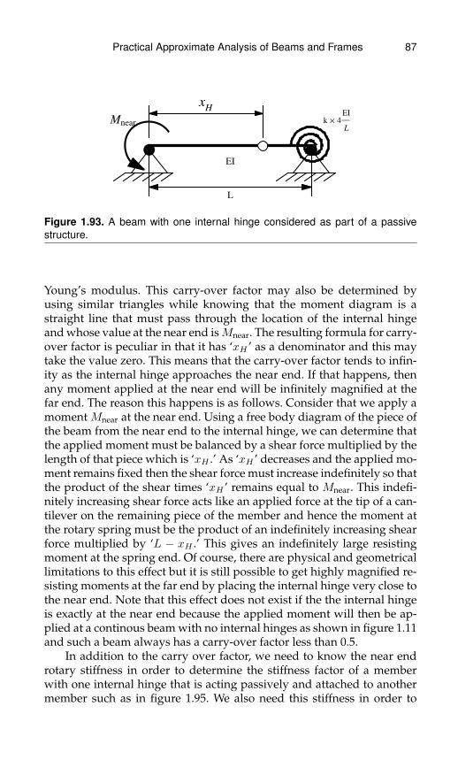
Practical Approximate Analysis of Beams and Frames 87
EI
L
xH
Mnear k ´ 4
EI
L
Figure 1.93. A beam with one internal hinge considered as part of a passivestructure.
Young’s modulus. This carry-over factor may also be determined byusing similar triangles while knowing that the moment diagram is astraight line that must pass through the location of the internal hingeand whose value at the near end isMnear. The resulting formula for carry-over factor is peculiar in that it has ‘xH ’ as a denominator and this maytake the value zero. This means that the carry-over factor tends to infin-ity as the internal hinge approaches the near end. If that happens, thenany moment applied at the near end will be infinitely magnified at thefar end. The reason this happens is as follows. Consider that we apply amoment Mnear at the near end. Using a free body diagram of the piece ofthe beam from the near end to the internal hinge, we can determine thatthe applied moment must be balanced by a shear force multiplied by thelength of that piece which is ‘xH .’ As ‘xH ’ decreases and the applied mo-ment remains fixed then the shear force must increase indefinitely so thatthe product of the shear times ‘xH ’ remains equal to Mnear. This indefi-nitely increasing shear force acts like an applied force at the tip of a can-tilever on the remaining piece of the member and hence the moment atthe rotary spring must be the product of an indefinitely increasing shearforce multiplied by ‘L − xH .’ This gives an indefinitely large resistingmoment at the spring end. Of course, there are physical and geometricallimitations to this effect but it is still possible to get highly magnified re-sisting moments at the far end by placing the internal hinge very close tothe near end. Note that this effect does not exist if the the internal hingeis exactly at the near end because the applied moment will then be ap-plied at a continous beam with no internal hinges as shown in figure 1.11and such a beam always has a carry-over factor less than 0.5.
In addition to the carry over factor, we need to know the near endrotary stiffness in order to determine the stiffness factor of a memberwith one internal hinge that is acting passively and attached to anothermember such as in figure 1.95. We also need this stiffness in order to

88 Practical Approximate Analysis of Beams and Frames
distribute an applied moment at a node that is connected to multiplemembers when one or more of these members has one internal hinge asin figure 1.96. The near end rotary stiffness factor is given by:
Mnear
θnear 4EI/L=
3k x2H
(3 + 4k)L2 − 6(L+ 2kL)xH + 3(1 + 4k)x2H
(1.9)
For any location of the internal hinge, this stiffness factor is always be-tween 0 and (3 + 4k)/(4 + 4k) ≤ 1. The minimum near end stiffnessfactor of zero is obtained when the internal hinge is infinitesimally closeto the near end while the maximum stiffness factor is obtained whenthe internal hinge is at the inflection point of a beam with no internalhinges but with the same spring at the far end. When the internal hingeis at the far end then the near end stiffness factor is always 0.75 becausethe beam becomes effectively freely hinged at the far end. Also, whenxH > (3+4k)/(3+8k), then the near end stiffness factor is always greateror equal to 0.75. In practice, we can use this as follows. When the stiff-ness factor ‘k’ is greater or equal to 0.75 then as long as the internal hingeis within L/3 (ie. one third the length) away from the spring end thenwe can take the near end stiffness factor to be approximately 1 instead ofsome value between 0.75 and 1 which, as was seen in previous examples,leads to good approximate results.
The formula for the near end stiffness factor 1.9 is relatively complexand so we will present it graphically. Figure 1.94 shows a contour plotof the normalized near end stiffness factor. This figure shows contoursof the near end stiffness factor given by formula 1.9 divided by the nearend stiffness factor of an equivalent beam but with no internal hinge.We note that this normalized stiffness factor must be 1 when the internalhinge is located at the coresponding location of the inflection point in abeam with no internal hinge. The stiffness factor decreases as the internalhinge approaches the near end and increases as the stiffness factor of thefar end (ie. ‘k’) increases.
Having discussed the near end stiffness factor, we note that as the in-ternal hinge gets closer to the near end, the near end stiffness factor tendsto zero while the carry-over factor for the moment at the far end tends toinfinity. If we have a structure as shown in figure 1.95, then the momentat B depends on the near end stiffness factor of member BC while the mo-ment at C is the product of the moment at B multiplied by the carry-overfactor for moments of member BC. It is then natural to ask which has thestronger effect, the stiffness factor at the near end or the carry-over factorfor moments? If we multiply the near end stiffness factor given in for-mula 1.9 by the carry-over factor given in formula 1.8 and we considerthe limit as the internal hinge approaches the near end then we find that

Practical Approximate Analysis of Beams and Frames 89
0.01
0.05
0.1
0.2
0.3
0.4
0.5
0.6
0.70.8
0.8
0.9 0.9
0.950.95
1
1
0.1 0.2 0.3 0.4 0.5 0.6 0.7 0.8 0.9 1.
xH
L
0.
0.5
1.
1.5
2.
2.5
3.
3.5
4.
k
Countours ofHMnear�ΘnearLwith hinge
HMnear�ΘnearLno hinge
Figure 1.94. Contours of the normalized near end stiffness factor for the beamshown in figure 1.93.
the limit is zero. In other words, in figure 1.95, the moment at B and at Cwill both tend to zero as the internal hinge approaches node B.
Now we again consider the continuous beam shown in figure 1.95and consider what can be the worst effect of having an internal hingeon the moment at C. Our concern is of course with the possibly largecarry-over factor for moments in member BC due to the presence of theinternal hinge. Therefore, we ask where should we locate the internalhinge so that either the moment at B or at C is a maximum. The mo-ment at B is a maximum when the rotary stiffness at B is a maxi-mum and this occurs when the internal hinge is placed at the inflection
EI
L
EI
L
xH
k ´ 4
EI
L
Mapplied AB
C
Figure 1.95. Example of a beam with one internal hinge acting as a passivestructure in a continuous beam.

90 Practical Approximate Analysis of Beams and Frames
point of member BC if that member had no internal hinges. The mo-ment at C is a maximum when the location of the internal hinge is atxH ≈ (3 + 5k)L/(3 + 9k) (maximum error < 1.6%) and the maximumvalue is equal to
(3 + 4k +
√9 + 36k + 32k2
)/(6+10k) times larger than
for a similar beam but with no internal hinge. This last magnification fac-tor is always less than about 1.066. Therefore, we conclude that no matterwhere we place the internal hinge in member BC, the moment at C can-not be larger than about 6.6% what it would be if member BC had nointernal hinge. If the length of AB is allowed to vary from 0 to 10 timesthe length of member BC then the maximum increase in the moment at Ccannot be larger than about 32.5% and occurs when the length of mem-ber AB is 10 times that of BC. From this we deduce that when a memberwith one internal hinge is acting as a passive member and is attachedto other passive members on the left and right then the transmitted mo-ment across the member will, in general, not be much higher but may bemuch less than if that member had no internal hinge.
If a member with an internal hinge is acting passively but has anactive member attached at one end then the situation is different thenwhen both sides have passive members. As an example, we consider thestructure shown in figure 1.96 where a uniform load is applied on mem-ber DB which is then equivalent to having an applied momentMapplied onthe passive structure ABC. What is then the largest bending moment inmember BC at node B and and at node C? The bending moment at node Bon member BC is obtained by distributing the applied moment on thetwo members AB and BC according to their relative stiffness or stiffnessfactor at B. Specifically, if we call the stiffness factor of member BC at B tobe kBC (given by formula 1.9) and the ratio β = (EICL) / (EILC ) then thebending moment at node B in member BC equals Mapplied kBC/ (kBC + β).
EI
L
EICLC
xHk ´ 4
EI
L
D
A
B
C
⇔EI
L
EICLC
xHMapplied k ´ 4
EI
L
A
B
C
Figure 1.96. Example of a beam with one internal hinge attached to anothermember with an external moment applied at the common node.
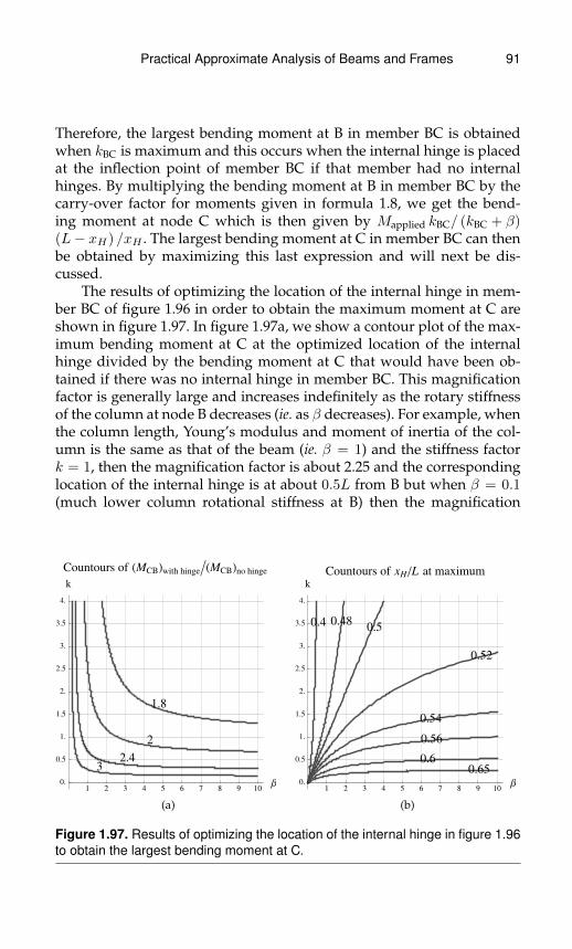
Practical Approximate Analysis of Beams and Frames 91
Therefore, the largest bending moment at B in member BC is obtainedwhen kBC is maximum and this occurs when the internal hinge is placedat the inflection point of member BC if that member had no internalhinges. By multiplying the bending moment at B in member BC by thecarry-over factor for moments given in formula 1.8, we get the bend-ing moment at node C which is then given by Mapplied kBC/ (kBC + β)(L− xH) /xH . The largest bending moment at C in member BC can thenbe obtained by maximizing this last expression and will next be dis-cussed.
The results of optimizing the location of the internal hinge in mem-ber BC of figure 1.96 in order to obtain the maximum moment at C areshown in figure 1.97. In figure 1.97a, we show a contour plot of the max-imum bending moment at C at the optimized location of the internalhinge divided by the bending moment at C that would have been ob-tained if there was no internal hinge in member BC. This magnificationfactor is generally large and increases indefinitely as the rotary stiffnessof the column at node B decreases (ie. as β decreases). For example, whenthe column length, Young’s modulus and moment of inertia of the col-umn is the same as that of the beam (ie. β = 1) and the stiffness factork = 1, then the magnification factor is about 2.25 and the correspondinglocation of the internal hinge is at about 0.5L from B but when β = 0.1(much lower column rotational stiffness at B) then the magnification
1.8
2
2.43
1 2 3 4 5 6 7 8 9 10Β0.
0.5
1.
1.5
2.
2.5
3.
3.5
4.
k
Countours of HMCBLwith hinge�HMCBLno hinge
(a)
0.4 0.480.5
0.52
0.54
0.56
0.60.65
1 2 3 4 5 6 7 8 9 10Β0.
0.5
1.
1.5
2.
2.5
3.
3.5
4.
k
Countours of xH�L at maximum
(b)
Figure 1.97. Results of optimizing the location of the internal hinge in figure 1.96to obtain the largest bending moment at C.
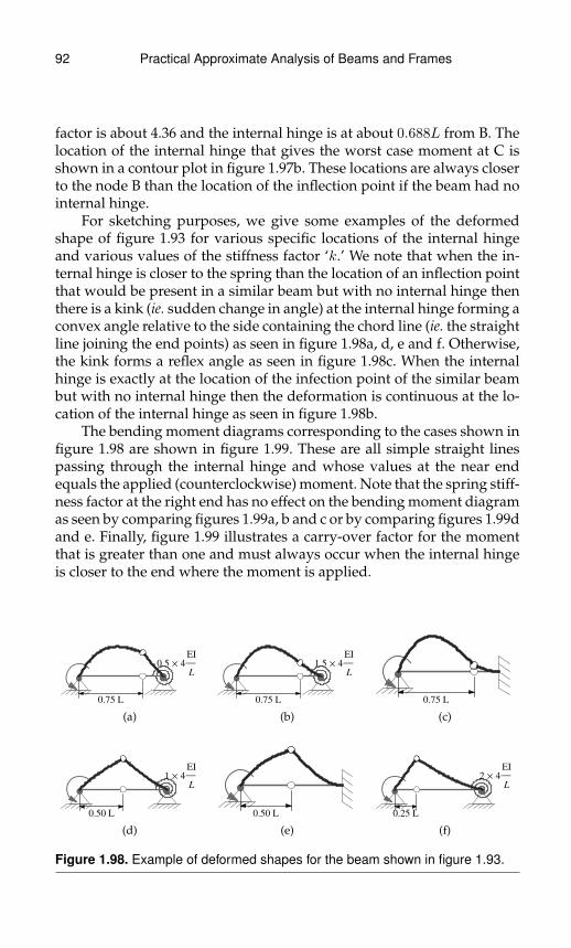
92 Practical Approximate Analysis of Beams and Frames
factor is about 4.36 and the internal hinge is at about 0.688L from B. Thelocation of the internal hinge that gives the worst case moment at C isshown in a contour plot in figure 1.97b. These locations are always closerto the node B than the location of the inflection point if the beam had nointernal hinge.
For sketching purposes, we give some examples of the deformedshape of figure 1.93 for various specific locations of the internal hingeand various values of the stiffness factor ‘k.’ We note that when the in-ternal hinge is closer to the spring than the location of an inflection pointthat would be present in a similar beam but with no internal hinge thenthere is a kink (ie. sudden change in angle) at the internal hinge forming aconvex angle relative to the side containing the chord line (ie. the straightline joining the end points) as seen in figure 1.98a, d, e and f. Otherwise,the kink forms a reflex angle as seen in figure 1.98c. When the internalhinge is exactly at the location of the infection point of the similar beambut with no internal hinge then the deformation is continuous at the lo-cation of the internal hinge as seen in figure 1.98b.
The bending moment diagrams corresponding to the cases shown infigure 1.98 are shown in figure 1.99. These are all simple straight linespassing through the internal hinge and whose values at the near endequals the applied (counterclockwise) moment. Note that the spring stiff-ness factor at the right end has no effect on the bending moment diagramas seen by comparing figures 1.99a, b and c or by comparing figures 1.99dand e. Finally, figure 1.99 illustrates a carry-over factor for the momentthat is greater than one and must always occur when the internal hingeis closer to the end where the moment is applied.
0.5 ´ 4
EI
L
0.75 L
(a)
1.5 ´ 4
EI
L
0.75 L
(b)0.75 L
(c)
1 ´ 4
EI
L
0.50 L
(d)0.50 L
(e)
2 ´ 4
EI
L
0.25 L
(f)
Figure 1.98. Example of deformed shapes for the beam shown in figure 1.93.

Practical Approximate Analysis of Beams and Frames 93
0.5 ´ 4
EI
L
0.75 L
(a)
1.5 ´ 4
EI
L
0.75 L
(b)0.75 L
(c)
1 ´ 4
EI
L
0.50 L
(d)
0.50 L
(e)
2 ´ 4
EI
L
0.25 L
(f)
Figure 1.99. Moment diagrams corresponding to the beams shown in figure 1.98.
1.13 Beam with One Internal Hingeand a Uniform Load
We now consider the case when a member with one internal hinge isattached on both ends to passive structures while being loaded over itsspan. In order for the member to be statically stable, at least one of thestiffness factors at the ends must be non-zero. When this condition ap-plies, then in general, such a loaded member has one inflection point.When we identify this inflection point then we can use statics in a man-ner similar to that shown in figure 1.30 or in figure 1.58 with one internalhinge replacing the role of the second inflection point. In addition, for-mulas 1.5 or formula 1.7 may then be used to determine the maximumpositive moment and the end moments for a uniform load and a pointforce load respectively with the location of the internal hinge replacingthe location of the second inflection point. We will start by discussing thecase of a uniform load.
For a uniform load on a beam with one internal hinge whose coor-dinate is ‘xH ,’ beam length ‘L’ and left and right stiffness factors ‘kL’and ‘kR’ respectively, there is one inflection point located at ‘xI ’ that isgiven by:
xI =kL(3 (L− xH) 2 + kR
(3L2 − 8LxH + 6x2
H
))3kR x2
H + kL
(3 (L− xH) 2 + 4kR
(L2 + 3xH (−L+ xH)
))L (1.10)
This formula is somewhat complex and involves three non-trivialindependent parameters all of which have non-negligible influence. Wenote that when other factors are fixed, the inflection point gets closer to
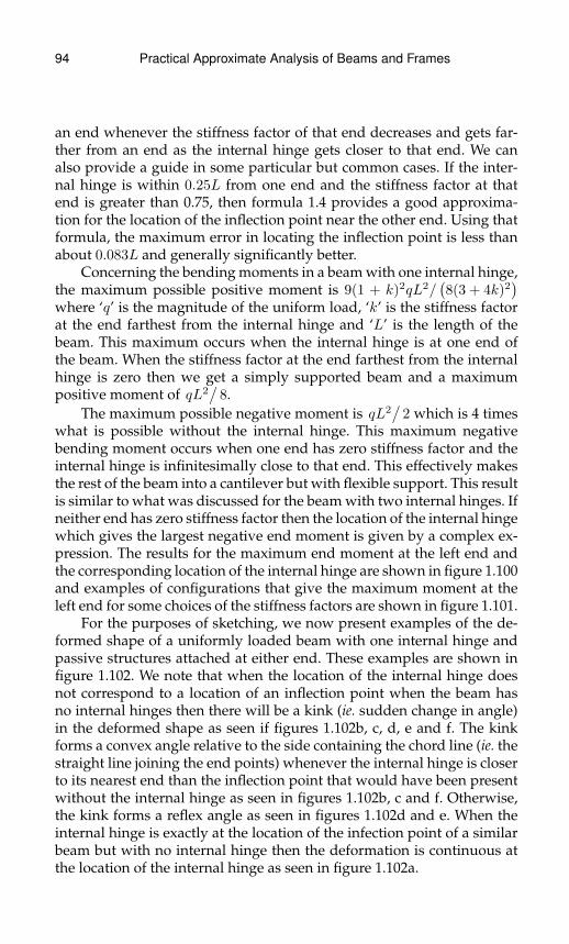
94 Practical Approximate Analysis of Beams and Frames
an end whenever the stiffness factor of that end decreases and gets far-ther from an end as the internal hinge gets closer to that end. We canalso provide a guide in some particular but common cases. If the inter-nal hinge is within 0.25L from one end and the stiffness factor at thatend is greater than 0.75, then formula 1.4 provides a good approxima-tion for the location of the inflection point near the other end. Using thatformula, the maximum error in locating the inflection point is less thanabout 0.083L and generally significantly better.
Concerning the bending moments in a beam with one internal hinge,the maximum possible positive moment is 9(1 + k)2qL2/
(8(3 + 4k)2
)where ‘q’ is the magnitude of the uniform load, ‘k’ is the stiffness factorat the end farthest from the internal hinge and ‘L’ is the length of thebeam. This maximum occurs when the internal hinge is at one end ofthe beam. When the stiffness factor at the end farthest from the internalhinge is zero then we get a simply supported beam and a maximumpositive moment of qL2
/8.
The maximum possible negative moment is qL2/
2 which is 4 timeswhat is possible without the internal hinge. This maximum negativebending moment occurs when one end has zero stiffness factor and theinternal hinge is infinitesimally close to that end. This effectively makesthe rest of the beam into a cantilever but with flexible support. This resultis similar to what was discussed for the beam with two internal hinges. Ifneither end has zero stiffness factor then the location of the internal hingewhich gives the largest negative end moment is given by a complex ex-pression. The results for the maximum end moment at the left end andthe corresponding location of the internal hinge are shown in figure 1.100and examples of configurations that give the maximum moment at theleft end for some choices of the stiffness factors are shown in figure 1.101.
For the purposes of sketching, we now present examples of the de-formed shape of a uniformly loaded beam with one internal hinge andpassive structures attached at either end. These examples are shown infigure 1.102. We note that when the location of the internal hinge doesnot correspond to a location of an inflection point when the beam hasno internal hinges then there will be a kink (ie. sudden change in angle)in the deformed shape as seen if figures 1.102b, c, d, e and f. The kinkforms a convex angle relative to the side containing the chord line (ie. thestraight line joining the end points) whenever the internal hinge is closerto its nearest end than the inflection point that would have been presentwithout the internal hinge as seen in figures 1.102b, c and f. Otherwise,the kink forms a reflex angle as seen in figures 1.102d and e. When theinternal hinge is exactly at the location of the infection point of a similarbeam but with no internal hinge then the deformation is continuous atthe location of the internal hinge as seen in figure 1.102a.

Practical Approximate Analysis of Beams and Frames 95
0.4
0.7 1 1.1
1.2
1.3
1.4
1.61.8
0.5 1. 1.5 2. 2.5 3. 3.5 4.kL
0.5
1.
1.5
2.
2.5
3.
3.5
4.
kR
Contours of maximum end moment � HqL2�8L
(a)
0.25
0.3
0.35
0.4
0.45
0.5
0.55
0.5 1. 1.5 2. 2.5 3. 3.5 4.kL
0.5
1.
1.5
2.
2.5
3.
3.5
4.
kR
Contours of xH�L for
maximum moment at left end
(b)
Figure 1.100. Maximum moment at the left end and corresponding locations ofthe internal hinge for a uniformly loaded beam as a function of the end stiffnessfactors.
0.40 L
0.01 ´ 4
EI
L
0.01 ´ 4
EI
L
0.302 L
(a)
0.41 L
1 ´ 4
EI
L
1 ´ 4
EI
L
0.325 L
(b)
0.42 L
0.347 L
(c)
0.36 L
1 ´ 4
EI
L
4 ´ 4
EI
L
0.379 L
(d)
0.46 L
4 ´ 4
EI
L
1 ´ 4
EI
L
0.285 L
(e)
0.79 L
0.01 ´ 4
EI
L
0.101 L
(f)
Figure 1.101. Locations of the internal hinge that give the maximum end momentat the left end for specific choices of the end stiffness factors when the beam isloaded by a uniform load.
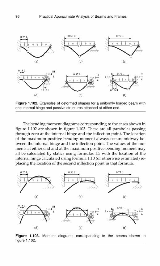
96 Practical Approximate Analysis of Beams and Frames
0.25 L
(a)
0.50 L
(b)
0.75 L
(c)
0.15 L
1 ´ 4
EI
L
0.115 L
(d)
0.85 L
4 ´ 4
EI
L
(e)
0.70 L
1 ´ 4
EI
L
2 ´ 4
EI
L
0.154 L
(f)
Figure 1.102. Examples of deformed shapes for a uniformly loaded beam withone internal hinge and passive structures attached at either end.
The bending moment diagrams corresponding to the cases shown infigure 1.102 are shown in figure 1.103. These are all parabolas passingthrough zero at the internal hinge and the inflection point. The locationof the maximum positive bending moment always occurs midway be-tween the internal hinge and the inflection point. The values of the mo-ments at either end and at the maximum positive bending moment mayall be calculated by statics using formulas 1.5 with the location of theinternal hinge calculated using formula 1.10 (or otherwise estimated) re-placing the location of the second inflection point in that formula.
0.25 L
(a)
0.50 L
(b)
0.75 L
(c)
0.15 L
1 ´ 4
EI
L
(d)
0.85 L
4 ´ 4
EI
L
(e)
0.70 L
1 ´ 4
EI
L
2 ´ 4
EI
L
(f)
Figure 1.103. Moment diagrams corresponding to the beams shown infigure 1.102.
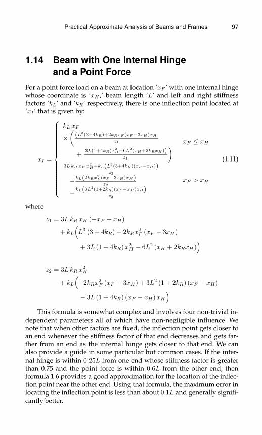
Practical Approximate Analysis of Beams and Frames 97
1.14 Beam with One Internal Hingeand a Point Force
For a point force load on a beam at location ‘xF ’ with one internal hingewhose coordinate is ‘xH ,’ beam length ‘L’ and left and right stiffnessfactors ‘kL’ and ‘kR’ respectively, there is one inflection point located at‘xI ’ that is given by:
xI =
kL xF
×(
(L3(3+4kR)+2kRxF (xF−3xH)xH
z1
+3L(1+4kR)x2
H−6L2(xH+2kRxH))z1
) xF ≤ xH
3LkR xF x2H+kL(L3(3+4kR)(xF−xH))
z2
−kL(2kRx2F (xF−3xH)xH)z2
−kL(3L2(1+2kR)(xF−xH)xH)z2
xF > xH
(1.11)
where
z1 = 3LkR xH (−xF + xH)
+ kL
(L3 (3 + 4kR) + 2kRx
2F (xF − 3xH)
+ 3L (1 + 4kR)x2H − 6L2 (xH + 2kRxH)
)z2 = 3LkR x
2H
+ kL
(−2kRx
2F (xF − 3xH) + 3L2 (1 + 2kR) (xF − xH)
− 3L (1 + 4kR) (xF − xH)xH
)This formula is somewhat complex and involves four non-trivial in-
dependent parameters all of which have non-negligible influence. Wenote that when other factors are fixed, the inflection point gets closer toan end whenever the stiffness factor of that end decreases and gets far-ther from an end as the internal hinge gets closer to that end. We canalso provide a guide in some particular but common cases. If the inter-nal hinge is within 0.25L from one end whose stiffness factor is greaterthan 0.75 and the point force is within 0.6L from the other end, thenformula 1.6 provides a good approximation for the location of the inflec-tion point near the other end. Using that formula, the maximum error inlocating the inflection point is less than about 0.1L and generally signifi-cantly better.
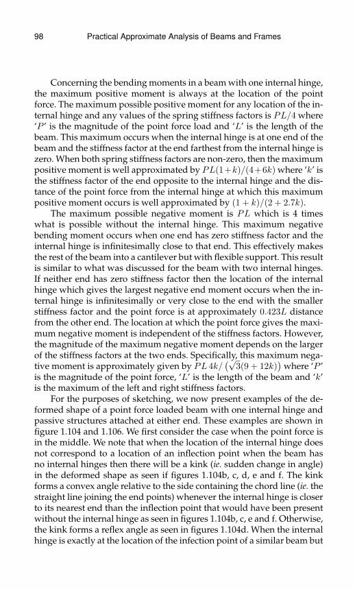
98 Practical Approximate Analysis of Beams and Frames
Concerning the bending moments in a beam with one internal hinge,the maximum positive moment is always at the location of the pointforce. The maximum possible positive moment for any location of the in-ternal hinge and any values of the spring stiffness factors is PL/4 where‘P ’ is the magnitude of the point force load and ‘L’ is the length of thebeam. This maximum occurs when the internal hinge is at one end of thebeam and the stiffness factor at the end farthest from the internal hinge iszero. When both spring stiffness factors are non-zero, then the maximumpositive moment is well approximated by PL(1+k)/(4+6k) where ‘k’ isthe stiffness factor of the end opposite to the internal hinge and the dis-tance of the point force from the internal hinge at which this maximumpositive moment occurs is well approximated by (1 + k)/(2 + 2.7k).
The maximum possible negative moment is PL which is 4 timeswhat is possible without the internal hinge. This maximum negativebending moment occurs when one end has zero stiffness factor and theinternal hinge is infinitesimally close to that end. This effectively makesthe rest of the beam into a cantilever but with flexible support. This resultis similar to what was discussed for the beam with two internal hinges.If neither end has zero stiffness factor then the location of the internalhinge which gives the largest negative end moment occurs when the in-ternal hinge is infinitesimally or very close to the end with the smallerstiffness factor and the point force is at approximately 0.423L distancefrom the other end. The location at which the point force gives the maxi-mum negative moment is independent of the stiffness factors. However,the magnitude of the maximum negative moment depends on the largerof the stiffness factors at the two ends. Specifically, this maximum nega-tive moment is approximately given by PL 4k/
(√3(9 + 12k)
)where ‘P ’
is the magnitude of the point force, ‘L’ is the length of the beam and ‘k’is the maximum of the left and right stiffness factors.
For the purposes of sketching, we now present examples of the de-formed shape of a point force loaded beam with one internal hinge andpassive structures attached at either end. These examples are shown infigure 1.104 and 1.106. We first consider the case when the point force isin the middle. We note that when the location of the internal hinge doesnot correspond to a location of an inflection point when the beam hasno internal hinges then there will be a kink (ie. sudden change in angle)in the deformed shape as seen if figures 1.104b, c, d, e and f. The kinkforms a convex angle relative to the side containing the chord line (ie. thestraight line joining the end points) whenever the internal hinge is closerto its nearest end than the inflection point that would have been presentwithout the internal hinge as seen in figures 1.104b, c, e and f. Otherwise,the kink forms a reflex angle as seen in figures 1.104d. When the internalhinge is exactly at the location of the infection point of a similar beam but

Practical Approximate Analysis of Beams and Frames 99
0.27 L
0.50 L
(a)
0.50 L
0.50 L
0.500 L
(b)
0.75 L
0.50 L
0.500 L
(c)
0.15 L
0.50 L4 ´ 4
EI
L
1 ´ 4
EI
L
0.158 L
(d)
0.50 L
0.50 L4 ´ 4
EI
L
1 ´ 4
EI
L
0.500 L
(e)
0.75 L
0.50 L4 ´ 4
EI
L
1 ´ 4
EI
L
0.260 L
(f)
Figure 1.104. Examples of deformed shapes for a point force loaded beam withone internal hinge and passive structures attached at either end.
with no internal hinge then the deformation is continuous at the locationof the internal hinge as seen in figure 1.104a. An additional observationis that the internal hinge divides the beam into two pieces. The piece thatis free of the point force behaves like a cantilever with flexible supportunless the stiffness factor on its side is zero (ie. regular hinge) and thenit simply rotates rigidly as seen in figure 1.104b and c. The piece that hasthe point force will, in general, have both positive and negative curva-tures but a maximum displacement occurs in that hinge only if that pieceis signficantly longer than the other as seen in figures 1.104a and d. Thisis due to the much higher flexibility of a cantilever relative to a beamwith some type of support at each end.
The bending moment diagrams corresponding to the cases shown infigure 1.104 are shown in figure 1.105. These are all piecewise straightlines passing through zero at the internal hinge and, when it exists,the inflection point. The location of the maximum positive bending mo-ment, if present, always occurs at the location of the point force as infigures 1.105a, d and f. In some cases, there is no maximum positive mo-ment because all the bending moments are negative or zero as seen infigure 1.105b, c and e. This occurs when the piece that is free of the pointforce has a zero stiffness factor at its end or when the point force is ap-plied exactly at the internal hinge. When the last case occurs then bothsides behave like cantilevers with flexible support and the shape alwayslooks similar to figure 1.105e except that the relative magnitudes at the

100 Practical Approximate Analysis of Beams and Frames
0.27 L
0.50 L
(a)
0.50 L
0.50 L
(b)
0.75 L
0.50 L
(c)
0.15 L
0.50 L4 ´ 4
EI
L
1 ´ 4
EI
L
(d)
0.50 L
0.50 L4 ´ 4
EI
L
1 ´ 4
EI
L
(e)
0.75 L
0.50 L4 ´ 4
EI
L
1 ´ 4
EI
L
(f)
Figure 1.105. Moment diagrams corresponding to the beams shown in fig-ure 1.104.
ends may differ. The values of the moments at either end and at the max-imum positive bending moment may all be calculated by statics usingformulas 1.7 with the location of the internal hinge calculated using for-mula 1.11 (or otherwise estimated) replacing the location of the secondinflection point in that formula.
The case when the point force is nearer to one end is similar to thecase when the point force is at the middle. Again, we note that whenthe location of the internal hinge does not correspond to a location ofan inflection point when the beam has no internal hinges then there willbe a kink (ie. sudden change in angle) in the deformed shape as seen iffigures 1.106a, b, c, e and f. The kink forms a convex angle relative to theside containing the chord line (ie. the straight line joining the end points)whenever the internal hinge is closer to its nearest end than the inflectionpoint that would have been present without the internal hinge as seen infigures 1.106a, b, c and e. Otherwise, the kink forms a reflex angle asseen in figure 1.106f. When the internal hinge is exactly at the location ofthe infection point of a similar beam but with no internal hinge then thedeformation is continuous at the location of the internal hinge as seen infigure 1.106d. Again as in the case when the point force is in the middle,the piece of the beam from the internal hinge to a support that is free ofthe point force behaves like a cantilever with flexible support unless thestiffness factor on its side is zero (ie. regular hinge) and then it simplyrotates rigidly as seen in figure 1.106a, b and c. The piece that has thepoint force will, in general, have both positive and negative curvaturesbut a maximum displacement occurs in that hinge only if that piece is
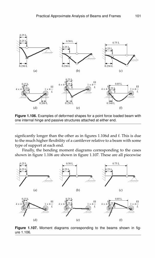
Practical Approximate Analysis of Beams and Frames 101
0.25 L
0.25 L
0.250 L
(a)
0.50 L
0.25 L
0.250 L
(b)
0.75 L
0.25 L
0.250 L
(c)
0.15 L
0.25 L4 ´ 4
EI
L
1 ´ 4
EI
L
0.200 L
(d)
0.25 L
0.25 L4 ´ 4
EI
L
1 ´ 4
EI
L
0.250 L
(e)
0.85 L
0.25 L4 ´ 4
EI
L
1 ´ 4
EI
L
0.148 L
(f)
Figure 1.106. Examples of deformed shapes for a point force loaded beam withone internal hinge and passive structures attached at either end.
signficantly longer than the other as in figures 1.106d and f. This is dueto the much higher flexibility of a cantilever relative to a beam with sometype of support at each end.
Finally, the bending moment diagrams corresponding to the casesshown in figure 1.106 are shown in figure 1.107. These are all piecewise
0.25 L
0.25 L
(a)
0.50 L
0.25 L
(b)
0.75 L
0.25 L
(c)
0.15 L
0.25 L4 ´ 4
EI
L
1 ´ 4
EI
L
(d)
0.25 L
0.25 L4 ´ 4
EI
L
1 ´ 4
EI
L
(e)
0.85 L
0.25 L4 ´ 4
EI
L
1 ´ 4
EI
L
(f)
Figure 1.107. Moment diagrams corresponding to the beams shown in fig-ure 1.106.

102 Practical Approximate Analysis of Beams and Frames
straight lines passing through zero at the internal hinge and, when it ex-ists, the inflection point. The location of the maximum positive bendingmoment, if present, always occurs at the location of the point force asin figures 1.105d, e and f. In some cases, there is no maximum positivemoment because all the bending moments are negative or zero as seenin figure 1.105a, b and c. This occurs when the piece that is free of thepoint force has a zero stiffness factor at its end or when the point forceis applied exactly at the internal hinge. When the last case occurs thenboth sides behave like cantilevers with flexible support and the shapealways looks similar to figure 1.107e except that the relative magnitudesat the ends may differ. The values of the moments at either end and atthe maximum positive bending moment may all be calculated by stat-ics using formulas 1.7 with the location of the internal hinge calculatedusing formula 1.11 (or otherwise estimated) replacing the location of thesecond inflection point in that formula.

Chapter 2
Approximate Analysis ofFrames with Sidesway
2.1 The Cantilever and theSingle Floor Portal Frame
In previous chapters, we have analyzed structures where the chord(ie. the line joining end points or nodes) of every member remains eitherat the same or at a parallel location relative to its original position. We saythat such structures have no sidesway. When a structure has sidesway,we will consider the effect of applying transverse point forces at only thenodes of members (ie. ends of members) with the effect of other loadsadded later through superposition. By using superposition it is possibleto include the effect of other loads that may be present.
The approximate analysis of structures with sidesway depends ona careful study of the stiffness of individual members relative to trans-verse motion or sidesway. We will call this stiffness the shear stiffness incontrast to the rotary stiffness that we considered previously. There areseveral ways that shear stiffness may be defined. For members that arefree of transverse loads on their span, we define the shear stiffness as theshear force in the member divided by the difference in transverse motionbetween the ends of the member. This definition is consistent becausethe shear force is uniform in such a member. We adopt this definitionbecause it is especially useful in analyzing buildings subject to sidesway.The reason is that the shear forces in columns of the same floor are thenproportional to their respective shear stiffnesses. This means that by de-termining or estimating the shear stiffness of columns, we can then de-termine the shear force in them. By estimating the shear force in columns,we can proceed to calculate or estimate end moments of all the membersin a structure subject to sidesway. Therefore, we will next study what
103
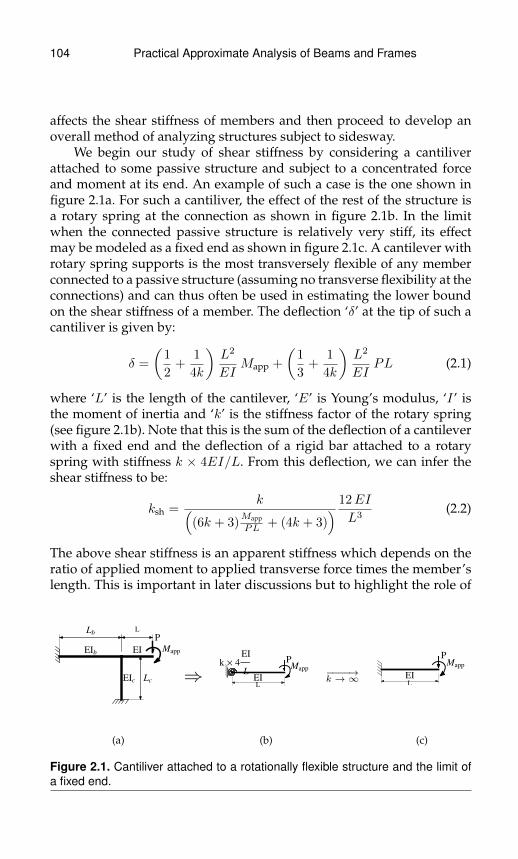
104 Practical Approximate Analysis of Beams and Frames
affects the shear stiffness of members and then proceed to develop anoverall method of analyzing structures subject to sidesway.
We begin our study of shear stiffness by considering a cantiliverattached to some passive structure and subject to a concentrated forceand moment at its end. An example of such a case is the one shown infigure 2.1a. For such a cantiliver, the effect of the rest of the structure isa rotary spring at the connection as shown in figure 2.1b. In the limitwhen the connected passive structure is relatively very stiff, its effectmay be modeled as a fixed end as shown in figure 2.1c. A cantilever withrotary spring supports is the most transversely flexible of any memberconnected to a passive structure (assuming no transverse flexibility at theconnections) and can thus often be used in estimating the lower boundon the shear stiffness of a member. The deflection ‘δ’ at the tip of such acantiliver is given by:
δ =
(1
2+
1
4k
)L2
EIMapp +
(1
3+
1
4k
)L2
EIPL (2.1)
where ‘L’ is the length of the cantilever, ‘E’ is Young’s modulus, ‘I’ isthe moment of inertia and ‘k’ is the stiffness factor of the rotary spring(see figure 2.1b). Note that this is the sum of the deflection of a cantileverwith a fixed end and the deflection of a rigid bar attached to a rotaryspring with stiffness k × 4EI/L. From this deflection, we can infer theshear stiffness to be:
ksh =k(
(6k + 3)Mapp
PL+ (4k + 3)
) 12EI
L3(2.2)
The above shear stiffness is an apparent stiffness which depends on theratio of applied moment to applied transverse force times the member’slength. This is important in later discussions but to highlight the role of
P
Mapp
L
EI
LcEIc
Lb
EIb
(a)
⇒k ´ 4
EI
L
PMapp
L
EI
(b)
−−−−→k →∞
PMapp
L
EI
(c)
Figure 2.1. Cantiliver attached to a rotationally flexible structure and the limit ofa fixed end.
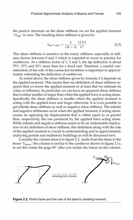
Practical Approximate Analysis of Beams and Frames 105
the passive structure on the shear stiffness we set the applied moment‘Mapp’ to zero. The resulting shear stiffness is given by:
ksh,P only =k
(4k + 3)
12EI
L3(2.3)
This shear stiffness is sensitive to the rotary stiffness, especially at stiff-ness factors between 0 and 3 which is expected to occur in practice forcantilevers. At a stiffness factor of 1, 2 and 3, the tip deflection is about75%, 37% and 25% more than for a fixed end. Therefore, a careful con-sideration of the role of the connected members is important in approxi-mately estimating the deflection of cantilevers.
As noted above, the shear stiffness given by formula 2.2 depends onthe applied moment. This means that our definition of shear stiffness re-quires that we know the applied moment or at least that we estimate itsvalue or influence. In particular, we can have an apparent shear stiffnessthat is either smaller or larger than when the applied force is acting alone.Specifically the shear stiffness is smaller when the applied moment isacting with the applied force and larger otherwise. It is even possible toget infinite shear stiffness as well as negative shear stiffness. The infiniteand negative stiffnesses occur when the applied moment, if acting alone,causes an opposing tip displacement that is either equal to or greaterthan, respectively, the one produced by the applied force acting alone.While infinite and negative stiffness seems to be an undesirable implica-tion of our definition of shear stiffness, this definition along with the roleof the applied moment is crucial in understanding and in approximatelyanalyzing portals and multistory buildings as will be discussed next.
Consider the column shown in figure 2.2. Aside from the shear in thebeam ‘Vbeam,’ the column is similar to the cantilever shown in figure 2.1c;to see this rotate the page 90◦ after you isolate the forces on the column.
−−−−−−−−−−−−→isolating left column
VcolumnMbeam
Vbeam
Figure 2.2. Portal frame and the role of the beam’s resisting moment.

106 Practical Approximate Analysis of Beams and Frames
When the deformations are small, the shear in the beam only causes anaxial force in the column. Also, the axial force in the beam has alreadybeen included in the shear in the column ‘Vcolumn.’ Therefore, the appar-ent shear stiffness of the column is given by formula 2.2 with ‘k’ → ∞,‘P ’ equal to the shear in the column ‘Vcolumn’ and the applied moment‘Mapp’ equal to the moment from the beam at the connection ‘Mbeam.’This moment ‘Mbeam’ acts to give a deformation in the opposite directionas the shear in the column ‘Vcolumn.’ Therefore, the shear stiffness of thecolumn will be larger with the beam than without it. Using equation 2.2with k →∞, the column shear stiffness is given by:
ksh,col =1(
6 MbeamVcolumn×Lcolumn
+ 4) 12EIcolumn
L3column
(2.4)
When the beam is extremely flexible, the moment in the beam is zero(ie. Mbeam = 0) and we find from formula 2.4 that the column shear stiff-ness is that of a cantilever which equals ‘3EIcolumn/L
3column.’ By contrast,
when the beam is infinitely stiff it prevents all rotation at the connectionwith the columns. In that case, both ends of the column cannot rotateand must, by symmetry, have the same bending moment. Since by stat-ics, the sum of the bending moments at the ends of a member with noloads on its span must equal the shear times the length of the member,we determine that the bending moment at the ends of each column willbe Mcolumn = (1/2) (Vcolumn × Lcolumn). By moment equilibrium (ie. stat-ics) at the connection between the column and the beam, we deduce thatMbeam = −Mcolumn = −(1/2) (Vcolumn × Lcolumn). With this value of mo-ment in the beam, we use formula 2.4 to determine that the column shearstiffness equals ‘12EIcolumn/L
3column.’ This stiffness is four times the stiff-
ness when the beam is extremely flexible. This shows that most of theshear stiffness of a portal is developed due to existence of the beams. Forthe passive portal frame shown in figure 2.2, the resisting moment de-veloped by the beam is between −1/2 and 0 so that the shear stiffness ofeach column is between one and four times the shear stiffness of a can-tilever. Although this provides valuable insight into the role of beamsin developing transverse stiffness in framed structures, we will prefer toconsider beams as providing rotary stiffness to the columns rather thanresisting moments in order to arrive at an effective approximate analysis.The reason is that it is easier to estimate a rotary stiffness (as describedpreviously) rather than to estimate a resisting moment and we need toestimate some parameters or variables in order to do an approximateanalysis.

Practical Approximate Analysis of Beams and Frames 107
P
LEI
Lbeam
EIbeam
(a)
⇒
k ´ 4
EI
LP
LEI
(b)
−−−−→k→∞
P
LEI
(c)
P
LEI
Lbeam
EIbeam
(d)
⇒
k ´ 4
EI
LP
LEI
(e)
−−−−→k→∞
P
LEI
(f)
Figure 2.3. Effect of a beam attached to a column is modeled as a rotary stiffness.
We now study the stiffness of a column that is hinged or fixed at thelower end and attached to a beam at the top as shown in figure 2.3. Ofcourse, the rotary stiffness of a beam or beams develop a resisting mo-ment which, for a fixed lower support, we can use formula 2.4 to deter-mine the column’s shear stiffness. However, we will develop a formulafor the shear stiffness of a column in terms of the rotary stiffness factor ofone or more attached beams. This rotary stiffness comes about when weremove an attached beam and replace it by its rotary stiffness as shownin figures 2.3b and e for the hinge and fixed supported columns respec-tively. In the limit of a very stiff beam, the rotary spring becomes equiva-lent to a sliding but non-rotating fixed end as shown in figures 2.3c and f.Here the rotary stiffness factor ‘k’ is calculated in the same way as in theframed structures with no sidesway. In the example of figure 2.3, the ro-tatry stiffness factor ‘k’ has the exact value of ( (EIbeam/Lbeam)/ (EI/L)).The shear stiffnesses for the column in figure 2.3b and e are given by:
ksh =
4k
(3+4k)3EIL3 hinge support (a)
(1+4k)(4+4k)
12EIL3 fixed support (b)
0 roller support (c)
(2.5)

108 Practical Approximate Analysis of Beams and Frames
The above shear stiffnesses are seen to be sensitive to the stiffness of theattached beam which increase with the stiffness of the attached beam.In particular, the column with the hinged end of figure 2.3a or equiv-alently 2.3b has zero stiffness if the beam has zero stiffness and hencedepends on the beam’s stiffness to provide any shear resistance. Forthe column with the fixed end of figure 2.3b, formula 2.5 indicates thatthe shear stiffness varies by a factor of 4 from 3EI
/L3 to 12EI
/L3 as
the stiffness of the attached beam varies from 0 to infinity. Note that ifmore than one beam is attached to the column then this result still ap-plies with the stiffness factor being the sum of the stiffness factors ofthe attached beams. Sample values for the shear stiffness for these twocases are given in table 2.1. As will be discussed later, the shear stiff-nesses of formulas 2.5 are sufficient to approximately analyze any multi-span, single floor portal subject to sidesway. However, to get good ac-curacy we must do a good estimate of the stiffness factors due to thebeams.
Table 2.1. Shear Stiffness of a Column that is Hingedor Fixed on One End and with Rotary Spring withStiffness Factor ‘k’ on Other End.
kshear/(EI/L3)
kshear/(EI/L3)
k (hinged end) (fixed end)
0.00 0.00 3.000.50 1.20 6.000.75 1.50 6.861.00 1.71 7.501.50 2.00 8.402.00 2.18 9.003.00 2.40 9.754.00 2.53 10.205.00 2.61 10.506.00 2.67 10.71∞ 3.00 12.00
In addition to the shear stiffness we will also need to calculate theend moments in the columns of figures 2.3a and d. We can express theseend moments in terms of the stiffness factors and the shear force inthe column. In addition, if needed, we can determine the location ofthe inflection point either in terms of the end moments using a sim-ple free-body-diagram or directly in terms of the stiffness factor of the

Practical Approximate Analysis of Beams and Frames 109
beam or beams. The end moments and location of the inflection pointare given by:(
Minner top
Minner bottom
)=
(2k
1+4k
− (1+2k)(1+4k)
)PL (fixed end) (2.6a)
and (Minner top
Minner bottom
)=
(1
0
)PL (hinged end) (2.6b)
xI =(1 + 2k)
(1 + 4k)L (fixed end) (2.6c)
andxI = 0 (or none) (hinged end) (2.6d)
where:
‘xI ’ is the location of the inflection point measured from the bottom and‘L’ is the length of the column.
Minner top and Minner bottom are the inner moments at the ends of the col-umn at the top and bottom respectively.
We consider Minner top and Minner bottom to be positive when counter-clockwise and clockwise respectively in conformance with standard con-ventions of bending moment diagrams.
Note that the difference between the bottom and top moment is al-ways equal to the shear in the column multiplied by the length (ie. PL).For a hinged support, there is no inflection point while for a fixed sup-port, the inflection point occurs between ‘0.5L’ and ‘0.6L’ when the stiff-ness factor is between 1 and ∞. Finally, for a roller support, the shearforce is zero and the bending moment is uniformly zero across the col-umn. A roller support in a column is equivalent to having no column atall in terms of shear stiffness.
While the structures shown in figure 2.3a and d are adequate for rep-resenting the columns of single floor portals, the behavior of beams in aportal are generally not passive. For example, in figure 2.4a, the existenceof a second column on the right exerts a clockwise moment on the rightend of the beam and this violates the assumption that the beam is act-ing with passive resistance. However, because of symmetry, there is aninflection point at the middle of the beam and this point remains at thesame level as the top of the columns. This means that the column on the

110 Practical Approximate Analysis of Beams and Frames
L
P=1
(a)
⇔
P=1
L�2
(b)
Figure 2.4. Simple portal frame and effective equivalent length of an attachedpassive beam.
left effectively sees a beam on a roller with half the length of the originalbeam as indicated in figure 2.4b. By considering both the reduced effec-tive length and the roller support, we conclude that the stiffness factorof the attached beam is 1.5 times the stiffness factor of a passive mem-ber that has the conditions of the ones shown in figures 2.3a and d. Forthis reason, in the approximate method to be described in a later section,we will magnify the stiffness factors of some of the beams connected tocolumns by this 1.5 factor.
If we want to study the effective stiffness factors of attached beamsmore carefully, we need to explicitly consider the effect of an active mo-ment applied on the far end of an attached beam. Consider a simple por-tal but with columns that may differ in their cross-sectional properties asshown in figure 2.5a. The action of the left column on the beam may bemodeled as shown in figure 2.5b. Our aim is to determine the effective
P
EI
Lbeam
EIbeam
LEIc2
(a)
−−−−−−−−−−−−−−−→beam apparent stiffnessrelative to left column
Mapplied Mfar end
Lbeam
EIbeam
(b)
Figure 2.5. Effect of far end resisting moment on the apparent stiffness factorsof attached beams.

Practical Approximate Analysis of Beams and Frames 111
rotary stiffness factor of such a beam relative to the left column when thefar end has a specified resisting moment ‘Mfar end.’ By solving the beamproblem shown in figure 2.5b, we can deduce:
kapparent =3
4− 2(Mfar end/Mapplied
) (2.7a)
or
kapparent =3 (xI/Lbeam)
6 (xI/Lbeam)− 2(2.7b)
where ‘xI ’ is the distance of the inflection point from the left end.We note that the apparent stiffness factor is 1 when the resisting
or far-end moment is half the applied one and this corresponds to anon-rotating end at the right side as is the case in figures 2.3a and d.Also the apparent stiffness factor is 1.5 when the ratio of far-end to ap-plied moment is 1 which corresponds to the symmetry case consideredin figure 2.4a. Therefore, formula 2.7a allows us to model both passiveand non-passive resisting beams using a rotary spring as shown in fig-ure 2.3e. However, for the purposes of doing an approximate analysis,we note that at the beginning of an analysis the far-end to near-end ap-plied moments in a beam are unknown and may be difficult to estimate.By contrast, the geometry and approximate ratios of sectional propertiesare either known or may be estimated and this allows us to estimate ro-tary stiffness factors under the assumption of passive resisting beams.For that reason, formula 2.7a is not very useful for approximate analy-sis except if we intend to use an iterative approach. In an iterative ap-proach, we start by assuming that the resisting beams are passive andobtain initial estimates for the end moments in all beams using the ap-proach outlined in the next section. With these estimated end moments,we can use formula 2.7a to obtain updated estimates of the stiffnessfactors for the beams and then proceed to do an updated approximateanalysis. This reanalysis may be done as many times as desired. How-ever, this approach is not recommended because the added complexityand effort of the iterative approach is generally not worth the improve-ment in accuracy and the convergence properties of such an iterativeapproach has not been fully studied. Instead of an iterative approach,we recommend use of 2.7a as a guide to make better initial estimatesof the stiffness factor of attached beams. For that purpose, its is instruc-tive to plot formulas 2.7a and 2.7b and these are shown in figures 2.6aand 2.7b.
The results shown in figure 2.6a and b indicate several interest-ing features. First, the effective rotary stiffness factor may be infinite
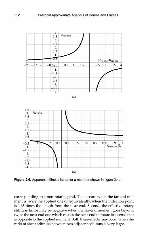
112 Practical Approximate Analysis of Beams and Frames
-2. -1.5 -1. -0.5 0.5 1. 1.5 2. 2.5 3. 3.5 4.
-4.
-3.5
-3.
-2.5
-2.
-1.5
-1.
-0.5
0.5
1.
1.5
2.
2.5
3.
3.5
4.
Mfar end�Mapplied
kapparent
(a)
0.1 0.2 0.3 0.4 0.5 0.6 0.7 0.8 0.9 1.
-4.
-3.5
-3.
-2.5
-2.
-1.5
-1.
-0.5
0.
0.5
1.
1.5
2.
2.5
3.
3.5
4.
4.5
xinflection�L
kapparent
(b)
Figure 2.6. Apparent stiffness factor for a member shown in figure 2.4b.
corresponding to a non-rotating end. This occurs when the far-end mo-ment is twice the applied one or, equivalently, when the inflection pointis 1/3 times the length from the near end. Second, the effective rotarystiffness factor may be negative when the far-end moment goes beyondtwice the near end one which causes the near-end to rotate in a sense thatis opposite to the applied moment. Both these effects may occur when theratio of shear stiffness between two adjacent columns is very large.

Practical Approximate Analysis of Beams and Frames 113
1 1.2 0.8 1.4
1
EI=2 EI=2.5 EI=1.8 EI=2.2
EI=1 EI=1.5 EI=1.2 EI=1.3 EI=1.8
P= 8
A B C DE
F G H I J
Figure 2.7. Single story sidesway example used to illustrate ideas.
In the next section, we will use the above study of the cantilever andportal and especially formula 2.5 to develop an effective approximatemethod to analyze any single story multi-span building subject to a sideforce. In subsequent sections, we will further study the response of a col-umn subject to sidesway in order to develop an effective approximatemethod for multi-story, multi-span buildings subject to side forces ap-plied at the nodes.
2.2 Approximate Analysis of Single FloorFrames Subject to a Horizontal Load
In the previous section, we have identified that formula 2.5 gives us theshear stiffness of a column with either a fixed or a hinged lower supportand beams attached at the top that are characterized by an effective ro-tary stiffness factor. We will use that formula to develop a method forsolving any single story multi-span building subject to a side force. Theoutline of the method is as follows:
1. Start by estimating the effective rotary stiffness factors at the top ofeach column.
2. Using the rotary stiffness factors, calculate the shear stiffness of eachcolumn using formula 2.5 reproduced below:
ksh =
4k
(3+4k)3EIL3 hinge support
(1+4k)(4+4k)
12EIL3 fixed support
0 roller support
Using the shear stiffness of each column, calculate the shear force ineach column by dividing the net applied side force at that level over
114 Practical Approximate Analysis of Beams and Frames
the columns in proportion to their shear stiffness. The net applied sideforce at a level is the total of all side forces that occur anywhere abovethe middle of the columns being considered.
3. Using formula 2.6, calculate the end moments and, optionally, the in-flection point in each column.
4. Knowing the moment at the top end of each column, apply those mo-ments as point moments on the nodes of the attached beams. Analyzethe resulting problem as a continuous beam with point moments onthe nodes but with no sidesway using the methods described previ-ously.
In the rest of this section, we will discuss each of the steps of theoutline specified above using figure 2.7 as a specific example.
Estimating rotary stiffness factors of beamsWe start by discussing how to estimate the rotary stiffness factors at thetop of each column. These factors are the sum of the stiffness factors ofthe beams attached to the top of the columns. The difficulty in accuratelyestimating these stiffness factors is due to the active nature of the beams.By active we mean that both ends of the beam are acted upon by theattached columns so that neither end behaves like a purely passive ro-tary spring. In the estimation process, we will discuss a simple approachthat gives generally good results (< 15% error in shear forces) but theerrors in some cases may be more. A more careful estimation of the ef-fective stiffness factor of the beams can give much more accurate results(< 10%) but with more effort. Ideas on how to do a more careful estima-tion will be discussed. However, we note that when the actual stiffnessfactor is greater than 1 and 2 respectively then the maximum error in es-timating the shear stiffness is about 42.9% and 27.3% respectively. Errorsin the shear stiffnesses in turn lead to less error in estimating the shearforces in the columns due to the distribution process with all factors be-ing less than one. Therefore, relatively large errors can only occur whenthe stiffness factor at the top of a column is less than 1 which rarely oc-curs in practical portals frames. In such cases, the large relative errors arelimited to the columns with low shear stiffness and these generally havemuch lower shear forces and end moments than the other columns andhence are less critical.
In the discussions, we will refer to the column under considerationas the self-column and the beams and columns to the left and right of theself column, if any, as the left beam, right beam, left column and rightcolumn respectively as shown in figure 2.8.
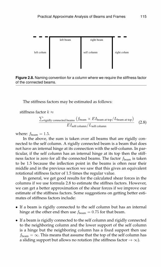
Practical Approximate Analysis of Beams and Frames 115
self column
left beam right beam
left colum right colum
Figure 2.8. Naming convention for a column where we require the stiffness factorof the connected beams.
The stiffness factors may be estimated as follows:
stiffness factor k ≈∑rigidly connected beams
(fbeam × EIbeam at top/Lbeam at top
)EIself column/Lself column
(2.8)
where: fbeam = 1.5.In the above, the sum is taken over all beams that are rigidly con-
nected to the self column. A rigidly connected beam is a beam that doesnot have an internal hinge at its connection with the self-column. In par-ticular, if the self column has an internal hinge at its top then the stiff-ness factor is zero for all the connected beams. The factor fbeam is takento be 1.5 because the inflection point in the beams is often near theirmiddle and in the previous section we saw that this gives an equivalentrotational stiffness factor of 1.5 times the regular value.
In general, we get good results for the calculated shear forces in thecolumns if we use formula 2.8 to estimate the stiffnes factors. However,we can get a better approximation of the shear forces if we improve ourestimate of the stiffness factors. Some suggestions on getting better esti-mates of stiffness factors include:
• If a beam is rigidly connected to the self column but has an internalhinge at the other end then use fbeam = 0.75 for that beam.
• If a beam is rigidly connected to the self column and rigidly connectedto the neighboring column and the lower support of the self columnis a hinge but the neighboring column has a fixed support then usefbeam =∞. This means that assume that the top of the self column hasa sliding support but allows no rotation (the stiffness factor→∞).

116 Practical Approximate Analysis of Beams and Frames
• If a beam is rigidly connected to the self column and to the neighbor-ing column and the lower support of the self column is fixed but theneighboring column has a hinge or roller support then use fbeam = 1.
Using the simple formula 2.8, we can generate the stiffness factors atthe top of each column for the structure shown in figure 2.7. The result isshown in table 2.2.
Table 2.2. Stiffness Factors at the Top of the Columns Shown in Figure 2.7.
Approximate analysis of a side loaded building
Preliminary calculations
Floor = 1
column 1 2 3 4 5
stiffness factor at top 3.000 4.083 5.417 0 0
stiffness factor at bottom ∞ 0 ∞ ∞ 0
Note that the stiffness factor of a column with a roller support at thebottom is always 0.
Calculating shear stiffness and shear forceOnce the stiffness factors of all the columns have been estimated, we candirectly calculate the shear stiffness of each column using formula 2.5.This is organized and presented in the row titled “shear stiffness” in ta-ble 2.3 with the total of the shear stiffness of all the columns shown in thelast column. Knowing the shear stiffness in the columns we can expressthe shear force in each column as the shear stiffness times the sideswayin that column. However, we note the following:
i) The difference between the sidesway of a column and its next neigh-bor is the axial deformation of the beam between them.
ii) Axial deformations in beams are much smaller than the sideswaybending deformations in columns. Therefore, we neglect the axialdeformations in beams.
These first two points imply that the sidesway of adjacent columnsare approximately the same.
iii) Since all columns in a portal are joined by beams and the sideswayof adjacent columns are approximately the same then the sideswayof all the columns in a portal are approximately the same.

Practical Approximate Analysis of Beams and Frames 117
From the above, we conclude that the shear force in each column isthe shear stiffness of that column times a sidesway which is the same forall the columns.
Next, we take a cut across all the columns at the bottom of thecolumns to get the free body diagram shown in figure 2.9. From this freebody diagram and taking the sum of forces in the horizontal direction,we deduce that the sum of the shear forces in all the columns equalsthe total side forces applied above the cut; in the example of figure 2.7and 2.9, the total is 8. Therefore, the total side forces equal the sum of theshear stiffnesses multiplied by the sidesway.
P=8
A B C D E
F G H I J
VAF
MAF bot
VBG
MBG bot
VCH
MCH bot
VDI
MDI bot
VEJ
MEJ bot
Figure 2.9. Free body diagram (excluding vertical axial forces) of figure 2.7 bytaking cut just above the supports.
Symbolically, if we call the sidesway ∆, then we can express the ar-gument described above symbolically as follows:
The total side forces equals the sum of the shear forces in the column:∑(side forces above cut) =
∑columns in floor
(shear force in column)
The sum of the shear forces is the sum of the shear stiffnesses multi-plied by the common sidesway:∑
columns in floor
(shear force in column) =∑
all columns
(ksh column ∆)
=
( ∑all columns
ksh column
)∆
Therefore, the total side forces above the cut equals the sum of shearstiffnesses multiplied by the common sidesway:∑
(side forces above cut) =
( ∑all columns
ksh column
)∆
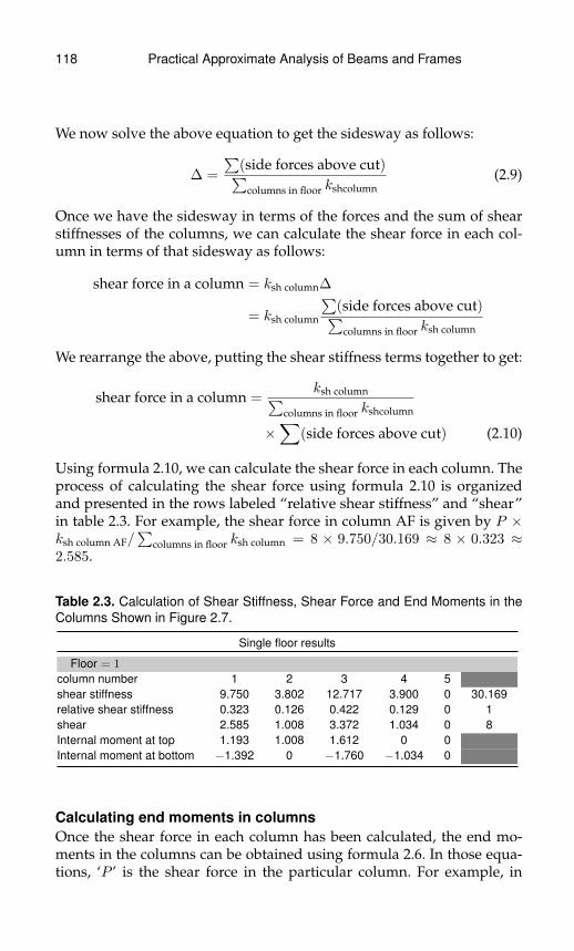
118 Practical Approximate Analysis of Beams and Frames
We now solve the above equation to get the sidesway as follows:
∆ =
∑(side forces above cut)∑
columns in floor kshcolumn(2.9)
Once we have the sidesway in terms of the forces and the sum of shearstiffnesses of the columns, we can calculate the shear force in each col-umn in terms of that sidesway as follows:
shear force in a column = ksh column∆
= ksh column
∑(side forces above cut)∑
columns in floor ksh column
We rearrange the above, putting the shear stiffness terms together to get:
shear force in a column =ksh column∑
columns in floor kshcolumn
×∑
(side forces above cut) (2.10)
Using formula 2.10, we can calculate the shear force in each column. Theprocess of calculating the shear force using formula 2.10 is organizedand presented in the rows labeled “relative shear stiffness” and “shear”in table 2.3. For example, the shear force in column AF is given by P ×ksh column AF/
∑columns in floor ksh column = 8 × 9.750/30.169 ≈ 8 × 0.323 ≈
2.585.
Table 2.3. Calculation of Shear Stiffness, Shear Force and End Moments in theColumns Shown in Figure 2.7.
Single floor results
Floor = 1
column number 1 2 3 4 5shear stiffness 9.750 3.802 12.717 3.900 0 30.169relative shear stiffness 0.323 0.126 0.422 0.129 0 1shear 2.585 1.008 3.372 1.034 0 8Internal moment at top 1.193 1.008 1.612 0 0Internal moment at bottom −1.392 0 −1.760 −1.034 0
Calculating end moments in columnsOnce the shear force in each column has been calculated, the end mo-ments in the columns can be obtained using formula 2.6. In those equa-tions, ‘P ’ is the shear force in the particular column. For example, in
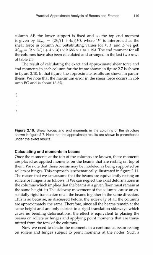
Practical Approximate Analysis of Beams and Frames 119
column AF, the lower support is fixed and so the top end momentis given by Mtop = (2k/(1 + 4k))PL where ‘P ’ is interpreted as theshear force in column AF. Substituting values for k, P and L we get:Mtop = (2 × 3/(1 + 4 × 3)) × 2.585 × 1 ≈ 1.193. The end moment for allthe columns have also been calculated and arranged in the last two rowsof table 2.3.
The result of calculating the exact and approximate shear force andend moments in each column for the frame shown in figure 2.7 is shownin figure 2.10. In that figure, the approximate results are shown in paran-thesis. We note that the maximum error in the shear force occurs in col-umn BG and is about 13.3%.
A B C D E
F G H I J
V=2.494
H2.585L
V=1.162
H1.008L
V=3.276
H3.372L
V=1.067
H1.034L
V=0.000
H0.000L
Mc=-1.379
H-1.392L
Mc=1.115
H1.193L
Mc=0.000
H0.000L
Mc=1.162
H1.008L
Mc=-1.749
H-1.760L
Mc=1.527
H1.612L
Mc=-1.067
H-1.034L
Mc=0.000
H0.000L
Mc=0.000
H0.000L
Mc=0.000
H0.000L
Figure 2.10. Shear forces and end moments in the columns of the structureshown in figure 2.7. Note that the approximate results are shown in parenthesesunder the exact results.
Calculating end moments in beamsOnce the moments at the top of the columns are known, these momentsare placed as applied moments on the beams that are resting on top ofthem. We note that those beams may be modeled as being supported onrollers or hinges. This approach is schematically illustrated in figure 2.11.The reason that we can assume that the beams are equivalently resting onrollers or hinges is as follows: i) We can neglect the axial deformations inthe columns which implies that the beams at a given floor must remain atthe same height. ii) The sideway movement of the columns cause an es-sentially rigid translation of all the beams together in the same direction.This is so because, as discussed before, the sidesway of all the columnsare approximately the same. Therefore, since all the beams remain at thesame height and are only subject to a rigid translation sideways whichcause no bending deformations, the effect is equivalent to placing thebeams on rollers or hinges and applying point moments that are trans-mitted from the tops of the columns.
Now we need to obtain the moments in a continuous beam restingon rollers and hinges subject to point moments at the nodes. Such a

120 Practical Approximate Analysis of Beams and Frames
col,1 col,2 col,3 col,4 col,5
P=8
↓ beams equivalentlyanalyzed as
Mtop col,1 Mtop col,2 Mtop col,3 Mtop col,4 = 0 Mtop col,5 = 0
Figure 2.11. Analyzing beams in portals as a continuous beam with no sidesway.
continuous beam has no sidesway and hence may be analyzed by themethods described in the previous chapter. However, due to the way theapplied moments are generated and because all the applied momentsare usually in the same sense, there’s a quick but less accurate way toestimate the end moments in the beams. This is simply to distribute theapplied moments at each node to the attached beams in proportion totheir relative nominal rotary bending stiffness. This approach usuallyworks because: i) for the extreme left and right ends of the continousbeam, the moments in the beams must match the applied moments andii) for internal nodes of the continuous beam, the influence of the appliedmoments on the left and right neighboring nodes have an opposing ef-fect to each other and therefore approximately cancel each other out. Ofcourse, this cancellation doesn’t always apply such as when the appliedmoments vary greatly from node to node. In that case, one must revertto the methods of the previous chapter.
Second example of portal frameAs a second example of the method presented, we consider the portalframe shown in figure 2.12. In this problem, we have an internal hinge inbeam HI near node H as well as column JE that has zero shear stiffnessdue to having both a hinge support and an internal hinge.
As in the previous example, we first prepare a table of the stiffnessfactors at the top of the columns as shown in table 2.4. Note that in thistable the stiffness factor of column EJ is zero because of the internal hinge
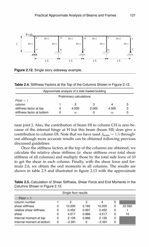
Practical Approximate Analysis of Beams and Frames 121
1.5 1.5 1.5 1.5
1
EI=2 EI=2 EI=2 EI=2
EI=1 EI=1 EI=1 EI=1 EI=1
P=10
A B C D E
F G H I J
Figure 2.12. Single story sidesway example.
Table 2.4. Stiffness Factors at the Top of the Columns Shown in Figure 2.12.
Approximate analysis of a side loaded building
Preliminary calculationsFloor = 1
column 1 2 3 4 5stiffness factor at top 0 4.000 2.000 4.000 0stiffness factor at bottom 0 ∞ 0 ∞ 0
near joint J. Also, the contribution of beam HI to column CH is zero be-cause of the internal hinge at H but this beam (beam HI) does give acontribution to column DI. Note that we have used fbeam = 1.5 through-out although more accurate results can be obtained following previousdiscussed guidelines.
Once the stiffness factors at the top of the columns are obtained, wecalculate the relative shear stiffness (ie. shear stiffness over total shearstiffness of all columns) and multiply those by the total side force of 10to get the shear in each column. Finally, with the shear force and for-mula 2.6, we obtain the end moments in all columns. The results areshown in table 2.5 and illustrated in figure 2.13 with the approximate
Table 2.5. Calculation of Shear Stiffness, Shear Force and End Moments in theColumns Shown in Figure 2.12.
Single floor results
Floor = 1column number 1 2 3 4 5shear stiffness 0 10.200 2.182 10.200 0 22.582relative shear stiffness 0 0.452 0.097 0.452 0 1shear 0 4.517 0.966 4.517 0 10Internal moment at top 0 2.126 0.966 2.126 0Internal moment at bottom 0 −2.391 0 −2.391 0

122 Practical Approximate Analysis of Beams and Frames
P=10
A B C D E
F G H I J
V=0.000
H0.000L
V=4.586
H4.517L
V=1.105
H0.966L
V=4.309
H4.517L
V=0.000
H0.000L
Mc=0.000
H0.000L
Mc=0.000
H0.000L
Mc=-2.486
H-2.391L
Mc=2.099
H2.126L
Mc=0.000
H0.000L
Mc=1.105
H0.966L
Mc=-2.394
H-2.391L
Mc=1.915
H2.126L
Mc=0.000
H0.000L
Mc=0.000
H0.000L
Figure 2.13. Shear forces and end moments in the columns of the structureshown in figure 2.12. Note that the approximate results are shown in parenthesesunder the exact results.
results shown in parenthesis below the exact results. The moments inthe beams have not been shown because these may be obtained usingthe methods discussed in the previous chapter.
2.3 Sketching Single Floor Portal FramesNow that we’ve discussed how to calculate the shear and bending mo-ments in the columns and beams of a structure subject to sidesway, weturn to the matter of sketching the deformed shape of such structures.In this regards, our objective is to identify the deformation patterns thatclarify how the overall structure distibutes the load and that illustratesthe relative stiffness of the members. We start with the column that has afixed lower support and that is subject to a side force which, by equilib-rium, must equal the internal shear force. As discussed before, the contri-bution of beams may be modeled as a rotary spring with stiffness factor‘k’ whose values range from zero to infinity. We will next discuss thedeformations of columns at some representative values of the stiffnessfactor of the beams and these are illustrated in figures 2.14a to f.
The case when the stiffness factor is zero corresponds to having aninternal hinge at the top of the column as for example is seen in col-umn DI in figure 2.7. In that case, the bending moment is zero at the topand has a value of ‘PL’ at the bottom where ‘P ’ is the applied force and‘L’ is the length of the column. If we rotate the page so that the chord ofthe column shown as a dashed line in figure 2.14a becomes horizontalthen we notice that this column becomes similar to a beam that is hingedat both ends and has an applied moment of ‘PL’ at one end. We’ve stud-ied this case before (see figure 1.14a) and we note that this member hasno inflection points. We also note that the rotation at the end where theload is applied is twice that at the other end but in the opposite senserelative to the horizontal. If we apply these observations to the columnof figure 2.14a, we deduce that the angle that the column makes relative
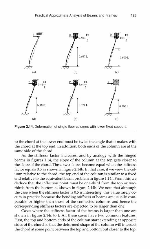
Practical Approximate Analysis of Beams and Frames 123
P
(a)
0.5´4
EI
L
P
0.667 L
(b)
1´4
EI
L
P
0.600 L
(c)
3´4
EI
L
P
0.538 L
(d)
5´4
EI
L
P
0.524 L
(e)
P
0.500 L
(f)
Figure 2.14. Deformation of single floor columns with lower fixed support.
to the chord at the lower end must be twice the angle that it makes withthe chord at the top end. In addition, both ends of the column are at thesame side of the chord.
As the stiffness factor increases, and by analogy with the hingedbeams in figures 1.14, the slope of the column at the top gets closer tothe slope of the chord. These two slopes become equal when the stiffnessfactor equals 0.5 as shown in figure 2.14b. In that case, if we view the col-umn relative to the chord, the top end of the column is similar to a fixedend relative to the equivalent beam problem in figure 1.14f. From this wededuce that the inflection point must be one-third from the top or two-thirds from the bottom as shown in figure 2.14b. We note that althoughthe case when the stiffness factor is 0.5 is interesting, this value rarely oc-curs in practice because the bending stiffness of beams are usually com-parable or higher than those of the connected columns and hence thecorresponding stiffness factors are expected to be larger than one.
Cases where the stiffness factor of the beams is larger than one areshown in figure 2.14c to f. All these cases have two common features.First, the top and bottom ends of the column start extending at oppositesides of the chord so that the deformed shape of the column will intersectthe chord at some point between the top and bottom but closer to the top.
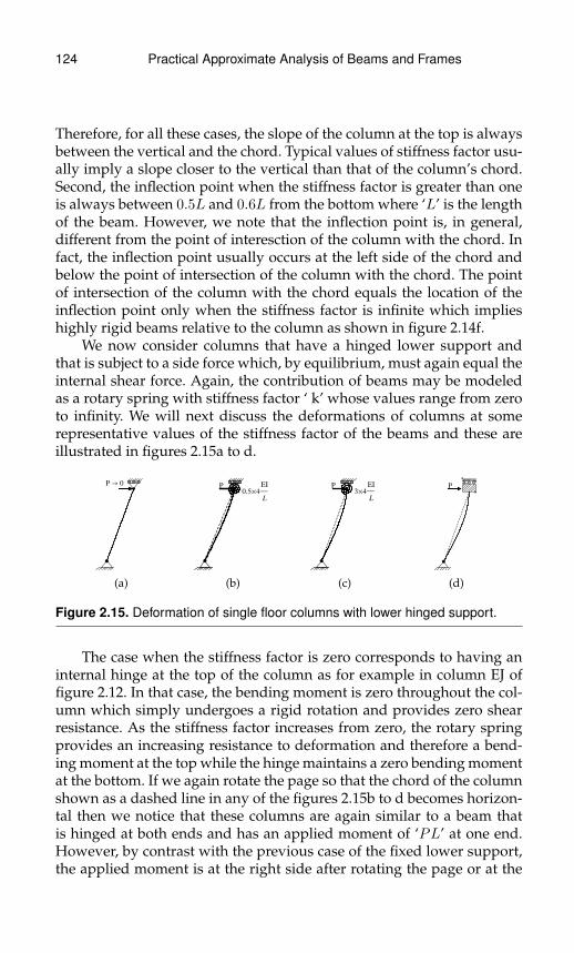
124 Practical Approximate Analysis of Beams and Frames
Therefore, for all these cases, the slope of the column at the top is alwaysbetween the vertical and the chord. Typical values of stiffness factor usu-ally imply a slope closer to the vertical than that of the column’s chord.Second, the inflection point when the stiffness factor is greater than oneis always between 0.5L and 0.6L from the bottom where ‘L’ is the lengthof the beam. However, we note that the inflection point is, in general,different from the point of interesction of the column with the chord. Infact, the inflection point usually occurs at the left side of the chord andbelow the point of intersection of the column with the chord. The pointof intersection of the column with the chord equals the location of theinflection point only when the stiffness factor is infinite which implieshighly rigid beams relative to the column as shown in figure 2.14f.
We now consider columns that have a hinged lower support andthat is subject to a side force which, by equilibrium, must again equal theinternal shear force. Again, the contribution of beams may be modeledas a rotary spring with stiffness factor ‘ k’ whose values range from zeroto infinity. We will next discuss the deformations of columns at somerepresentative values of the stiffness factor of the beams and these areillustrated in figures 2.15a to d.
P ® 0
(a)
0.5´4
EI
L
P
(b)
3´4
EI
L
P
(c)
P
(d)
Figure 2.15. Deformation of single floor columns with lower hinged support.
The case when the stiffness factor is zero corresponds to having aninternal hinge at the top of the column as for example in column EJ offigure 2.12. In that case, the bending moment is zero throughout the col-umn which simply undergoes a rigid rotation and provides zero shearresistance. As the stiffness factor increases from zero, the rotary springprovides an increasing resistance to deformation and therefore a bend-ing moment at the top while the hinge maintains a zero bending momentat the bottom. If we again rotate the page so that the chord of the columnshown as a dashed line in any of the figures 2.15b to d becomes horizon-tal then we notice that these columns are again similar to a beam thatis hinged at both ends and has an applied moment of ‘PL’ at one end.However, by contrast with the previous case of the fixed lower support,the applied moment is at the right side after rotating the page or at the
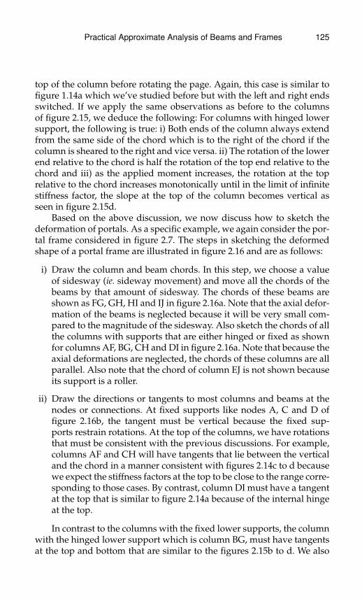
Practical Approximate Analysis of Beams and Frames 125
top of the column before rotating the page. Again, this case is similar tofigure 1.14a which we’ve studied before but with the left and right endsswitched. If we apply the same observations as before to the columnsof figure 2.15, we deduce the following: For columns with hinged lowersupport, the following is true: i) Both ends of the column always extendfrom the same side of the chord which is to the right of the chord if thecolumn is sheared to the right and vice versa. ii) The rotation of the lowerend relative to the chord is half the rotation of the top end relative to thechord and iii) as the applied moment increases, the rotation at the toprelative to the chord increases monotonically until in the limit of infinitestiffness factor, the slope at the top of the column becomes vertical asseen in figure 2.15d.
Based on the above discussion, we now discuss how to sketch thedeformation of portals. As a specific example, we again consider the por-tal frame considered in figure 2.7. The steps in sketching the deformedshape of a portal frame are illustrated in figure 2.16 and are as follows:
i) Draw the column and beam chords. In this step, we choose a valueof sidesway (ie. sideway movement) and move all the chords of thebeams by that amount of sidesway. The chords of these beams areshown as FG, GH, HI and IJ in figure 2.16a. Note that the axial defor-mation of the beams is neglected because it will be very small com-pared to the magnitude of the sidesway. Also sketch the chords of allthe columns with supports that are either hinged or fixed as shownfor columns AF, BG, CH and DI in figure 2.16a. Note that because theaxial deformations are neglected, the chords of these columns are allparallel. Also note that the chord of column EJ is not shown becauseits support is a roller.
ii) Draw the directions or tangents to most columns and beams at thenodes or connections. At fixed supports like nodes A, C and D offigure 2.16b, the tangent must be vertical because the fixed sup-ports restrain rotations. At the top of the columns, we have rotationsthat must be consistent with the previous discussions. For example,columns AF and CH will have tangents that lie between the verticaland the chord in a manner consistent with figures 2.14c to d becausewe expect the stiffness factors at the top to be close to the range corre-sponding to those cases. By contrast, column DI must have a tangentat the top that is similar to figure 2.14a because of the internal hingeat the top.
In contrast to the columns with the fixed lower supports, the columnwith the hinged lower support which is column BG, must have tangentsat the top and bottom that are similar to the figures 2.15b to d. We also

126 Practical Approximate Analysis of Beams and Frames
A
F
B
G
C
H
D
I J
(a) Sketch the chords (dashed lines)
A
F
B
G
C
H
D
I J
(b) Sketch directions at nodes wherever possible
A
F
B
G
C
H
D
I J
(c) Sketch the columns
Figure 2.16. Steps in sketching the deformed shape of problem 2.7.
note that column BG is attached to beams that are in turn attached tocolumns on either side that are relatively much more rigid column BG.This causes the inflection point in beams FG and GH to be closer to Gwhich gives an apparently high stiffness factors at the top of column BG.The result is that the tangent at the top of column BG will be close to thevertical and thus close to figure 2.15 which has no rotation at the top.
In order to draw the tangents to the beams, we first note that at rigidconnections, such as nodes F, G and H in figure 2.16b, the angles be-tween columns and beams must be maintained after the deformation.Since those connections were orthogonal (ie. 90◦) before the deformationthen the beams must remain orthogonal to the columns after the defor-mation and we correspondingly draw the tangent to the beams at those

Practical Approximate Analysis of Beams and Frames 127
A
F
B
G
C
H
D
I J
(d) Sketch the beams
A
F
B
G
C
H
D
I J
(e) Add column with rollers (rigid rotation)
A B C DE
F G H I J
(f) Remove extraneous lines (keep chord lines)
Figure 2.16. (continued): Steps in sketching the deformed shape of problem 2.7.
nodes as shown at nodes F, G and H of figure 2.16b. Second, the nodesthat are not rigidly connected to columns must deform in a manner con-sistent with the other beams and in view of the model of figure 2.11. Forexample, node I is not subjected to a moment transmitted from the topof the column and therefore will act passively in resisting the momenttransmitted from node H. This means that the rotation of the beams atnode I will be consistent with figure 1.11 with the moment at H viewedas the applied moment and with node I providing a passive rotary stiff-ness. Consequently, the beams at node I must have a rotation opposite tothe rotation of node H and with magnitude less than half the rotation atnode H. Finally, we have zero moment at node J because column EJ haszero shear stiffness and thus member IJ is similar to figure 1.14a. This

128 Practical Approximate Analysis of Beams and Frames
means the rotation at node J is exactly half the rotation at node I but inthe opposite sense than at node J. These are also sketched in figure 2.16balong with the tangent at J to column EJ being orthogonal to the tan-gent at J to beam IJ because the connection at J is rigid and beams IJ andcolumn EJ were orthogonal before the deformation.
iii) Draw the columns by using the tangents at the nodes and fig-ures 2.14 and 2.15 as a guide. The result of sketching these columnsare shown in figure 2.16c. We also add an ‘x’ marker at the approxi-mate location of the inflection points. Note that columns with fixedlower supports have inflection points whenever the top of the col-umn does not have an internal hinge while columns with a hingedsupport have no inflection points in all cases.
iv) Draw the beams by using the tangents at the nodes as a guide. Theresult of sketching these columns are shown in figure 2.16c. We alsoadd an ‘x’ marker at the approximate location of the inflection points.Note that inflection points are placed closer to the columns withlower shear stiffness.
v) Draw the column or columns with rollers using the tangents as aguide and knowing that those columns must be subject to a rigidrotation. The result of sketching the column is shown in figure 2.16e.
vi) Remove extraneous lines that were used in constructing the sketchin order to get a better looking drawing of the deformed shape. Inthis step, we recommend that the chords be kept because they helpto clarify the deformations of the columns and beams.
As a further example of sketching the deformation of portals sub-ject to sidesway we consider the problem shown in figure 2.12. The de-formed shape is shown in figure 2.17. Note that the steps in sketchingthe deformed shape is similar to the previous case. We start by sketching
P=10
A B C DE
F GH I J
Figure 2.17. Sketch deformed shape of problem 2.12.

Practical Approximate Analysis of Beams and Frames 129
the chords, followed by tangents at nodes and so on. Some of the newfeatures are as follows:
• Column EJ has a lower hing support and an internal hinge at the top.Its deformation follows figure 2.15a so that the column rotates as arigid beam.
• The internal hinge in beam HI at H implies that the tangent at H tobeam HI will not be orthogonal to the tangent a H to column CH afterdeformation. Node H of beam HI will have a rotation that is half therotation at node I because it behaves in a way similar to the beam infigure 1.14a which we’ve studied before but with the left and rightends switched.
• The internal hinge in the last column EJ implies that the moment inthe beam IJ at node J is also zero. This again implies that beam IJ willbehave like the beam in figure 1.14a with the rotation at node J beinghave the rotation at node I.
Other features such as the deformation of the columns BG, CH, DIand AF in figure 2.17 are similar to corresponding features in the previ-ous problem shown in figure 2.16.
Finally, having described how to sketch the deformation of portals,we note that this requires considerable knowledge of the deformationof various columns and beams as well as an estimation of the relativestiffness of different members. Consequently, as we sketch the deforma-tion of portals, we gain a better understanding of their overall behav-ior. Conversely, as we have more experience with portals, we can sketchtheir deformations with more precise features. Therefore, sketching thedeformation of portals or of structures with sidesway is an excellent ed-ucational tool because we gain a better understanding of the behavior ofportals and can demonstrate our increased understanding in ever moreprecise details that further enhances our understanding. Furthermore,we can quickly answer explorative design questions such as what hap-pens if a support is changed from being fixed to hinged or the effect ofadding an internal hinge at any given location.
2.4 The Column with Rotary Springsand Moments at Both Ends
Now that we have a method to approximately analyze a single storyportal frame, we will extend it to analyze multi-story frames subject tosidesway. At first, we might think that nothing more is needed and that
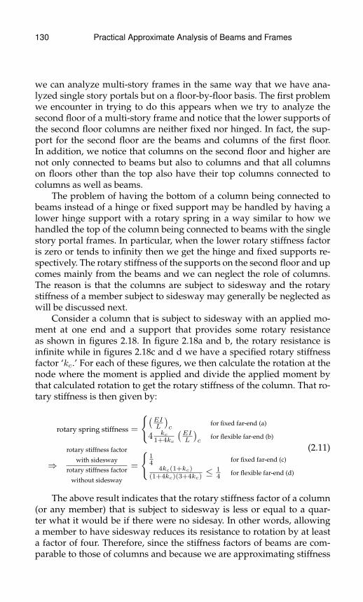
130 Practical Approximate Analysis of Beams and Frames
we can analyze multi-story frames in the same way that we have ana-lyzed single story portals but on a floor-by-floor basis. The first problemwe encounter in trying to do this appears when we try to analyze thesecond floor of a multi-story frame and notice that the lower supports ofthe second floor columns are neither fixed nor hinged. In fact, the sup-port for the second floor are the beams and columns of the first floor.In addition, we notice that columns on the second floor and higher arenot only connected to beams but also to columns and that all columnson floors other than the top also have their top columns connected tocolumns as well as beams.
The problem of having the bottom of a column being connected tobeams instead of a hinge or fixed support may be handled by having alower hinge support with a rotary spring in a way similar to how wehandled the top of the column being connected to beams with the singlestory portal frames. In particular, when the lower rotary stiffness factoris zero or tends to infinity then we get the hinge and fixed supports re-spectively. The rotary stiffness of the supports on the second floor and upcomes mainly from the beams and we can neglect the role of columns.The reason is that the columns are subject to sidesway and the rotarystiffness of a member subject to sidesway may generally be neglected aswill be discussed next.
Consider a column that is subject to sidesway with an applied mo-ment at one end and a support that provides some rotary resistanceas shown in figures 2.18. In figure 2.18a and b, the rotary resistance isinfinite while in figures 2.18c and d we have a specified rotary stiffnessfactor ‘kc.’ For each of these figures, we then calculate the rotation at thenode where the moment is applied and divide the applied moment bythat calculated rotation to get the rotary stiffness of the column. That ro-tary stiffness is then given by:
rotary spring stiffness =
{(EIL
)c
for fixed far-end (a)
4 kc1+4kc
(EIL
)c
for flexible far-end (b)
⇒
rotary stiffness factor
with sidesway
rotary stiffness factor
without sidesway
=
{14 for fixed far-end (c)
4kc(1+kc)(1+4kc)(3+4kc)
≤ 14
for flexible far-end (d)
(2.11)
The above result indicates that the rotary stiffness factor of a column(or any member) that is subject to sidesway is less or equal to a quar-ter what it would be if there were no sidesay. In other words, allowinga member to have sidesway reduces its resistance to rotation by at leasta factor of four. Therefore, since the stiffness factors of beams are com-parable to those of columns and because we are approximating stiffness
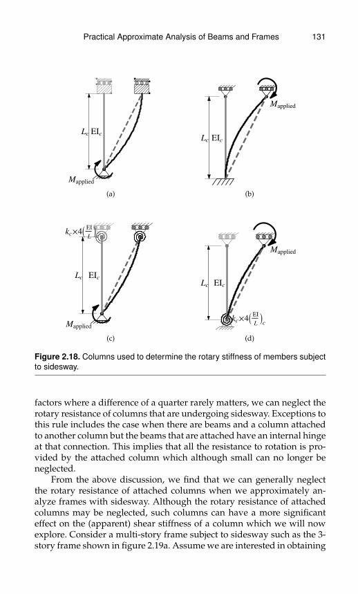
Practical Approximate Analysis of Beams and Frames 131
Mapplied
Lc EIc
(a)
Mapplied
Lc EIc
(b)
Mapplied
kc´4IEI
LMc
Lc EIc
(c)
kc´4IEI
LMc
Mapplied
Lc EIc
(d)
Figure 2.18. Columns used to determine the rotary stiffness of members subjectto sidesway.
factors where a difference of a quarter rarely matters, we can neglect therotary resistance of columns that are undergoing sidesway. Exceptions tothis rule includes the case when there are beams and a column attachedto another column but the beams that are attached have an internal hingeat that connection. This implies that all the resistance to rotation is pro-vided by the attached column which although small can no longer beneglected.
From the above discussion, we find that we can generally neglectthe rotary resistance of attached columns when we approximately an-alyze frames with sidesway. Although the rotary resistance of attachedcolumns may be neglected, such columns can have a more significanteffect on the (apparent) shear stiffness of a column which we will nowexplore. Consider a multi-story frame subject to sidesway such as the 3-story frame shown in figure 2.19a. Assume we are interested in obtaining

132 Practical Approximate Analysis of Beams and Frames
A B C D
E F G H
I J K L
M N O P
AAAA
EEEE
B CCCC
I
GG
DD
G
DD
M
H
MM
H
K
NN
LLL
O PPPP
AAA
E
B
EE
BB CCCCC
I
DD
G
D
M
HHH
MM
KK
NN
LL
O
L
O PP
BBBBBB
M
CC
(a)
−−−−→focus oncolumn FJ
F G
I J
(b)
−−−−→focus oncolumn J J
Mcol above
Mcolumn
Mbeam rightMbeam left
(c)
Figure 2.19. Effect of columns on their mutual shear stiffnesses.
the shear stiffness of column FJ in that figure. To that end, we isolate thatcolumn as shown in figure 2.19b. In that figure, we note the curvature ofthe beams and of the columns and beams attached to the top and bottomnodes of column FJ. These curvatures indicate that the bending momentsin the beams are resisting the deformation while the bending momentsin the columns are increasing the deformation. We can see this better ifwe isolate either node F or node J as shown in figure 2.19c and then referto the results associated with the cantilever of figure 2.1b. Physically, thereason that attached columns increase the deformation is because theyare also subject to shearing and are not simply passively resisting rota-tions.
So far, we have determined that beams that are attached at the topor at the bottom of columns help to resist deformations while similarlyattached columns help to increase the deformations. In order to translatethese observations into results we could use in an approximate analysis,we consider the column shown in figure 2.20. In that figure, the effectof attached beams are modeled as rotary springs both at the top and atthe bottom. The effective stiffness factor of these springs at either the topor bottom are determined in the same way that we determined the stiff-ness factor at the top of the single floor portal. The special case whenthe lower stiffness factor is zero or tends to infinity corresponds to thecolumn at the ground floor with either a hinge or a fixed support re-spectively. By contrast with the beams, the effect of an attached columneither at the top or at the bottom is modeled as an applied moment cor-responding to the bending moment at the connected end of the attachedcolumn. We note that these moments are applied on both the columnand the rotary springs which can be understood by considering the mo-ments on the nodes in figure 2.19c. For the special case when there is noattached column at a connection such as when we consider the bottomof a ground floor column or the top of a top floor column, then the corre-sponding applied moment must be zero. This means that with referenceto figure 2.20, Mt = 0 at a top floor column and Mb = 0 at a ground floor
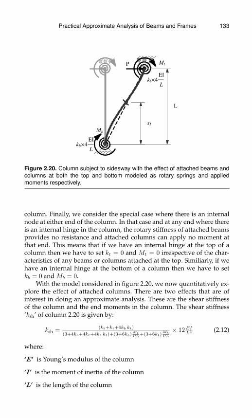
Practical Approximate Analysis of Beams and Frames 133
kb´4EI
L
Mb
kt´4EI
L
MtP
xI
L
Figure 2.20. Column subject to sidesway with the effect of attached beams andcolumns at both the top and bottom modeled as rotary springs and appliedmoments respectively.
column. Finally, we consider the special case where there is an internalnode at either end of the column. In that case and at any end where thereis an internal hinge in the column, the rotary stiffness of attached beamsprovides no resistance and attached columns can apply no moment atthat end. This means that if we have an internal hinge at the top of acolumn then we have to set kt = 0 and Mt = 0 irrespective of the char-acteristics of any beams or columns attached at the top. Similiarly, if wehave an internal hinge at the bottom of a column then we have to setkb = 0 and Mb = 0.
With the model considered in figure 2.20, we now quantitatively ex-plore the effect of attached columns. There are two effects that are ofinterest in doing an approximate analysis. These are the shear stiffnessof the column and the end moments in the column. The shear stiffness‘ksh’ of column 2.20 is given by:
ksh = (kb+kt+4kb kt)
(3+4kb+4kt+4kb kt)+(3+6kb)MtPL +(3+6kt)
MbPL
× 12EIL3 (2.12)
where:
‘E’ is Young’s modulus of the column
‘I’ is the moment of inertia of the column
‘L’ is the length of the column

134 Practical Approximate Analysis of Beams and Frames
‘kb’ and ‘kt’ are the stiffness factors at the top and bottom respectively
‘P ’ is the shear in the column with P positive according to the conven-tion of figure 2.20
‘Mb’ and ‘Mt’ are the moments applied at the top and bottom respec-tivley with clockwise moments being positive.
We note that, as required, formula 2.12 reduces to formula 2.5a whenkt = k, kb = 0, Mb = Mt = 0 and to formula 2.5b when kt = k, kb → ∞,Mb = Mt = 0. Also, we note that clockwise applied moments at ei-ther the top or the bottom will increase the denominator in formula 2.12which will therefore decrease the (apparent) shear stiffness of the col-umn. Such clockwise moments are in the same sense as the momentsthat attached columns would apply on the top and on the bottom con-nections. Therefore, we generally expect our estimates of shear stiffnessto decrease when we include the effect of attached columns versus whenwe neglect them. We will explore this matter quantitatively for groundfloor, middle floor and top floor columns separately.
Ground floor columns in a multistory frame have columns attachedonly at their tops. We expect that these attached columns will have endmoments that are comparable to the ground floor ones and hence weexpect that Mt/PL . 0.5. The lower support of ground columns areeither fixed or hinged but in either case the moment at the bottom iszero (ie. Mb = 0). We then plot in figures 2.21a and b the percentage de-crease in stiffness for the fixed and hinge support respectively as a func-tion of Mt/PL and for various values of the effective stiffness factor ofthe top beams. Figures 2.21 indicate that when Mt/PL ≤ 0.5 then thedecrease in stiffness is less than about 40% in all cases. While this max-imum is considerable, we note that all the columns in the ground floor
0.1 0.2 0.3 0.4 0.5 0.6 0.7 0.8 0.9 1.
Mt�HPLL
10
20
30
40
50
60
Dksh�ksh%
Stiffness decrease; bottom fixed
kt = 6
kt = 3
kt = 2
kt = 1
kt = 0
(a)
0. 0.1 0.2 0.3 0.4 0.5 0.6 0.7 0.8 0.9 1.
Mt�HPLL
5
10
15
20
25
30
35
40
45
50
Dksh�ksh%
Stiffness decrease; bottom hinged
kt = 6
kt = 3
kt = 2
kt = 1
kt = 10-9
(b)
Figure 2.21. Stiffness decrease in ground floor columns due to attached columnsat their top.

Practical Approximate Analysis of Beams and Frames 135
will generally have a comparable decrease and we need to accurately es-timate the relative shear stiffness rather than the absolute shear stiffness.This means that the maximum error in estimating the shear stiffness willtranslate into a much lower error in estimating the shear forces as will beobserved in the examples in the next section. In any case, the estimates ofthe shear force will improve in a second iteration when we use estimatesof Mt/PL obtained from the results of the first iteration.
Top floor columns in a multistory frame have columns attachedonly at their bottom ends. We expect that these attached columns willhave end moments that are comparable to the top floor ones, henceMb/PL . 0.5. The top of top columns are, by definition, not attachedto columns and hence the applied moment at the top is zero (ie. Mt = 0).We then plot the percentage decrease in stiffness as a function of Mb/PLand for various values of the effective stiffness factor of the bottombeams for two typical values of the stiffness factor of the beams at thetop, specifically with kt = 1 and 3 for figures 2.22a and b respectively.Figures 2.22 indicate that when Mt/PL ≤ 0.5 then the decrease in stiff-ness is less than about 40% in all cases. While this maximum is consid-erable, we note that all the columns in the top floor will generally havea comparable decrease and we need to accurately estimate the relativeshear stiffness rather than the absolute shear stiffness. This means thatthe maximum error in estimating the shear stiffness will translate into amuch lower error in estimating the shear forces as will be observed in theexamples in the next section. In any case, the estimates of the shear forcewill improve in a second iteration when we use estimates of Mb/PLobtained from the results of the first iteration.
Middle floor columns in a multistory frame have columns attachedat both their top and bottom ends. We expect that these attached columnswill have end moments that are comparable to their own moments attheir ends and hence Mt/PL ≈ Mb/PL . 0.5. We then plot the per-centage decrease in stiffness as a function of Mt/PL ≈ Mb/PL andfor various values of the effective stiffness factor at the bottom and topbeams which we have taken to be approximately the same in figure 2.23a.That figure indicates that when Mt/PL ≈ Mb/PL ≤ 0.5 then the de-crease in stiffness is less than about 50% in all cases. While this maxi-mum is considerable, we note that all the columns in the middle floorwill generally have a comparable decrease and we need to accurately es-timate the relative shear stiffness rather than the absolute shear stiffness.This means that the maximum error in estimating the shear stiffness willtranslate into a much lower error in estimating the shear forces as will beobserved in the examples in the next section. In any case, the estimates ofthe shear force will improve in a second iteration when we use estimatesof end moments obtained from the results of the first iteration. We have
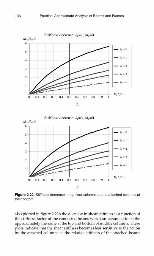
136 Practical Approximate Analysis of Beams and Frames
0. 0.1 0.2 0.3 0.4 0.5 0.6 0.7 0.8 0.9 1.
Mb�HPLL
10
20
30
40
50
60
Dksh�ksh%
Stiffness decrease; kt=1, Mt=0
kb = 6
kb = 3
kb = 2
kb = 1
kb = 0
(a)
0. 0.1 0.2 0.3 0.4 0.5 0.6 0.7 0.8 0.9 1.
Mb�HPLL
10
20
30
40
50
60
Dksh�ksh%
Stiffness decrease; kt=3, Mt=0
kb = 6
kb = 3
kb = 2
kb = 1
kb = 0
(b)
Figure 2.22. Stiffness decrease in top floor columns due to attached columns attheir bottom.
also plotted in figure 2.23b the decrease in shear stiffness as a function ofthe stiffness factor of the connected beams which are assumed to be theapproximately the same at the top and bottom of middle columns. Theseplots indicate that the shear stiffness becomes less sensitive to the actionby the attached columns as the relative stiffness of the attached beams

Practical Approximate Analysis of Beams and Frames 137
0. 0.1 0.2 0.3 0.4 0.5 0.6 0.7 0.8 0.9 1.
Mt�HPLL=Mb�HPLL5
10
15
20
25
30
35
40
45
50
55
60
65
70
Dksh�ksh%
Stiffness decrease; kb = kt
k = 6
k = 3
k = 2
k = 1
k = 10-9
(a)
0. 0.5 1. 1.5 2. 2.5 3. 3.5 4.
kt = kb
5
10
15
20
25
30
35
40
45
50
Dksh�ksh%
Stiffness decrease; Mt=Mb
M�PL=0.5
M�PL=0.4
M�PL=0.3
M�PL=0.2
M�PL=0.1
(b)
Figure 2.23. Stiffness decrease in top floor columns due to attached columns attheir bottom.
increases. The reason is that these attached beams will absorb more ofthe moment applied by the attached columns and will therefore have areduced effect on the shear stiffness of the column.
The second effect that is of interest in doing an approximate anal-ysis is an expression for the end moments of column 2.20. These end
138 Practical Approximate Analysis of Beams and Frames
moments are given by:(Minner top
Minner bottom
)=
(+ kt+2kbktkb+kt+4kbkt
− kb+2kbktkb+kt+4kbkt
)PL+
(+ ktkb+kt+4kbkt
+ ktkb+kt+4kbkt
)Mb
+
(− kbkb+kt+4kbkt
− kbkb+kt+4kbkt
)Mt
(2.13)
Note that in the above formulas, the applied moments Mt and Mb areconsidered positive when clockwise and the applied load P is consid-ered positive when acting to the right. By contrast, the inner bendingmoments Minner top and Minner bottom are considered to be positive whencounterclockwise and clockwise respectively in conformance with stan-dard conventions of bending moment diagrams.
By inspective formula 2.13 we find that it reduces to formula 2.6awhen kt = k, kb → ∞, Mb = Mt = 0 and to formula 2.6b when kt = k,kb = 0, Mb = Mt = 0. Formula 2.13 gives the end moments as the linearsuperposition of the effect of each of the transverse force P , the appliedmoment at the top Mt and the applied moment at the bottom Mb. If weonly apply a moment at one of the ends (ie. onlyMb or onlyMt), the shearforce in the member must be zero and therefore the column must be ina state of pure bending. This means that the bending moment in the col-umn is the same throughout the column. By considering moment equi-librium at the node where the moment is applied, we note that the uni-form bending moment plus the moment in the spring must equal the ap-plied moment. This means that the applied moment must be distributedaccording to the relative stiffness of the rotary spring versus the rotary re-sistance of the column. The rotary resistance of a column subject to sides-way is given by formula 2.11b. For example, for the moment applied atthe bottom, the moment in the column and spring must be in proportionto kt/ (1 + 4kt) versus kb. The bending moment in the column is thengiven by (kt/ (1 + 4kt)) / ((kt/ (1 + 4kt)) + kb) = kt/ (kb + kt + 4kbkt) asindicated by the second terms of formula 2.13. The effect of the appliedmoment at the top may be similarly verified.
The way that the applied moments affect the column indicates thatthese will have a relatively small contribution. That will generally be truebecause the rotary stiffness of a column subject to sidesway will havea relatively low stiffness (as discussed in the context of formula 2.11)relative to the attached beams. For an approximate analysis, this meansthat most of the error in estimating the bending moments at the endsof a column will be due to errors in estimating the shear force in thecolumn and therefore indirectly due to estimating the shear stiffness ofthe column.

Practical Approximate Analysis of Beams and Frames 139
Related to the end moments is the location of the inflection pointbecause we can deduce that location from the end moments. The locationof the inflection point measured from the bottom is given by:
xI = (kb+2kbkt)−kt(Mb/(PL))+kb(Mt/(PL))(kb+kt+4kbkt)
L (on condition 0 ≤ xI ≤ L)(2.14)
We note that, as required, formula 2.13 reduces to formula 2.6c whenkb → ∞. Also, when kb and kt are both greater than one, which is theusual case, the inflection point is always between 0.4L and 0.6L whenMb = Mt = 0. The effect of Mb and Mt act against each other so that Mb
causes the inflection point to shift down while Mt causes the inflectionpoint to shift up. However, in any case, the effect ofMb andMt on the in-flection point location is small for the same reason that their effect on theend moments are small (see previous discussion). However, it is possiblefor unusually large values of Mb or Mt to cause the column to have noinflection point at all. Although the conditions for this are unusual, thesecan sometimes occur in a large number of floors multistory building ateither the top floor where Mb is acting alone and may be relatively largeor the ground floor where Mt is acting alone and may be relatively large.
2.5 Approximate Analysis of Multiple FloorFrames Subject to Horizontal Loads
In the previous section, we have identified that formula 2.12 gives us theshear stiffness of any column in a multi-story building with the attachedbeams at the top and bottom modeled by effective rotary stiffness factorsand the attached columns modeled by applied moments. In addition, wehave formula 2.13 which gives us the end moments in each column whengiven the same kind of information. We will use these two formulas todevelop a method for solving any multi-story building subject to a sideforce. The outline of the method is as follows:
1. Start by estimating the effective rotary stiffness factors at the top andbottom of each column at every floor. Note that the ground floor isspecial so that the lower spring factor is taken to be infinite for a fixedsupport or zero for a hinge support. Equivalently, we can use formula2.5 for the ground floor columns.
2. In a first iteration, assume that columns do not apply moments on eachother (ie. Mb = Mt = 0 in formulas 2.12 and 2.13) and then use therotary stiffness factors from step 1 to calculate the shear stiffness ofeach column using formula 2.12.

140 Practical Approximate Analysis of Beams and Frames
Using the shear stiffness of each column and with each floor consid-ered separately, calculate the shear force in each column of a specificfloor by dividing the net applied side force above that floor over thecolumns in that floor in proportion to their shear stiffness. The net ap-plied side force at a floor is the total of all side forces that occur any-where above the middle of the columns of the floor being considered.
3. Using formula 2.13, calculate the end moments and, optionally, usingformula 2.14 calculate the inflection point in each column.
4. At this point, we have estimated the moments at the top and bottomof each column. If we now isolate a node or connection joining oneor more beams with one or more columns, the moments applied bythe columns at a node are known. Because these column moments areknown, we can apply their algebraic sum as a point moment appliedon the beams at the nodes. To get the beam end moments at a givenfloor, we then analyze all the beams at that floor as a continuous beamwith no sidesway and with known point moments on the nodes ap-plied by the columns. This problem may be approximately analyzedusing the methods described in the previous chapter.
5. In a second optional iteration, use the end moments in the columnsobtained from step 3 as an estimate of what moment to apply on thecolumns attached to them (ie. estimates of Mb and Mt). Again use for-mula 2.12 to calculate an updated shear stiffness for each column.
Using the updated shear stiffness of each column and on each floorconsidered separately, calculate the shear force in the same manner asin step 2.
6. Repeat step 3 but with the updated shear force and applied moments.
7. Repeat step 4 but with updated estimates of column moments.
In the rest of this section, we will illustrate most of the steps of theoutline specified above using figure 2.24 as a specific example.
The first step is to estimate the effective rotary stiffness of the beamson the ends of each column. This is done in the same way we did the sin-gle floor portal with two new considerations. First, columns have othercolumns attached to them as well as beams. In each case and based onprevious discussions, we simply neglect the rotary stiffness provided bythe columns. For example, at the top of column AD, the rotary stiffnessfactor is 1.5 × (EIDE/LDE) / (EIAD/LAD) = 1.5 × (2/5)/(2/4) = 1.2.We note that we neglect the stiffness of column DG when obtainingthis stiffness factor and the multiplier 1.5 is the same multiplier used
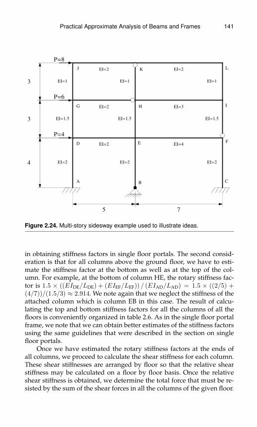
Practical Approximate Analysis of Beams and Frames 141
5 7
4
3
3
EI=2
EI=2
EI=2
EI=4
EI=3
EI=2
EI=2
EI=1.5
EI=1
EI=2
EI=1.5
EI=1
EI=2
EI=1.5
EI=1
P=4
P=6
P=8
A B C
D E F
G H I
J K L
Figure 2.24. Multi-story sidesway example used to illustrate ideas.
in obtaining stiffness factors in single floor portals. The second consid-eration is that for all columns above the ground floor, we have to esti-mate the stiffness factor at the bottom as well as at the top of the col-umn. For example, at the bottom of column HE, the rotary stiffness fac-tor is 1.5 × ((EIDE/LDE) + (EIEF/LEF)) / (EIAD/LAD) = 1.5 × ((2/5) +(4/7))/(1.5/3) ≈ 2.914. We note again that we neglect the stiffness of theattached column which is column EB in this case. The result of calcu-lating the top and bottom stiffness factors for all the columns of all thefloors is conveniently organized in table 2.6. As in the single floor portalframe, we note that we can obtain better estimates of the stiffness factorsusing the same guidelines that were described in the section on singlefloor portals.
Once we have estimated the rotary stiffness factors at the ends ofall columns, we proceed to calculate the shear stiffness for each column.These shear stiffnesses are arranged by floor so that the relative shearstiffness may be calculated on a floor by floor basis. Once the relativeshear stiffness is obtained, we determine the total force that must be re-sisted by the sum of the shear forces in all the columns of the given floor.

142 Practical Approximate Analysis of Beams and Frames
Table 2.6. Stiffness Factors at the Top of the Columns Shown in Figure 2.24.
Approximate analysis of a side loaded building
Preliminary calculations
Floor = 1column 1 2 3stiffness factor at top 1.200 2.914 1.714stiffness factor at bottom ∞ 0 ∞
Floor = 2column 1 2 3stiffness factor at top 1.200 1.286 1.286stiffness factor at bottom 1.200 2.914 0
Floor = 3column 1 2 3stiffness factor at top 1.800 0 1.286stiffness factor at bottom 1.800 1.929 1.929
For example, for the second floor of figure 2.24, we consider the free bodydiagram, with axial forces omitted for aesthetics, shown in figure 2.25.From figure 2.25, we determine that the total force to be resisted by theshear forces in the second floor columns is 8 + 6 = 14. This total force isthen multipied by the relative shear stiffness to obtain the shear force ineach column in that second floor. This process is done for each floor andthe calculations and results are conveniently organized in table 2.7. Inthat table, in addition to the shear force in each column of each floor, we
P=6
P=8
DE
F
G H
I
JK
L
VDG
MDG bot
VEH
MEH bot
VFI
MFI bot
= 0
Figure 2.25. Free body diagram (excluding vertical axial forces) of figure 2.24 bytaking a cut just above the first floor beams.

Practical Approximate Analysis of Beams and Frames 143
Table 2.7. First Iteration Calculations of Shear Stiffness, Shear Force and EndMoments in the Columns Shown in Figure 2.24.
Iteration number = 1
Floor = 1column number 1 2 3shear stiffness 0.247 0.075 0.271 0.593relative shear stiffness 0.417 0.126 0.458 1shear 7.501 2.263 8.236 18Internal moment at top 12.415 9.051 14.376Internal moment at bottom −17.589 0 −18.569
Floor = 2column number 1 2 3shear stiffness 0.296 0.368 0.105 0.769relative shear stiffness 0.385 0.478 0.137 1shear 5.392 6.692 1.916 14Internal moment at top 8.088 9.186 5.747Internal moment at bottom −8.088 −10.890 0
Floor = 3column number 1 2 3shear stiffness 0.242 0.080 0.226 0.549relative shear stiffness 0.442 0.146 0.413 1shear 3.533 1.166 3.301 8Internal moment at top 5.300 0 4.708Internal moment at bottom −5.300 −3.498 −5.193
also calculate the bending moment at the top and bottom of each columnof each floor using 2.13 with Mb = Mt = 0.
Once we are done with the first iteration, we may do a second itera-tion. To decide whether a second iteration is needed we note the follow-ing:
• In general, the first iteration will give an adequate approximation fora preliminary analysis. If we evaluate the error in the shear force ofthe columns with the largest such values in each floor then the relativeerrors in the first iteration will be about 10% to 30%.
• The relative error in all columns decreases as the stiffness contrast be-tween columns in the same floor decreases.
• A second iteration generally improves the results by a relative error ofabout 10% to 15%.
• Relatively low errors of less than about 5% to 10% in all columns can beachieved only if we carefully estimate and update the rotary stiffness
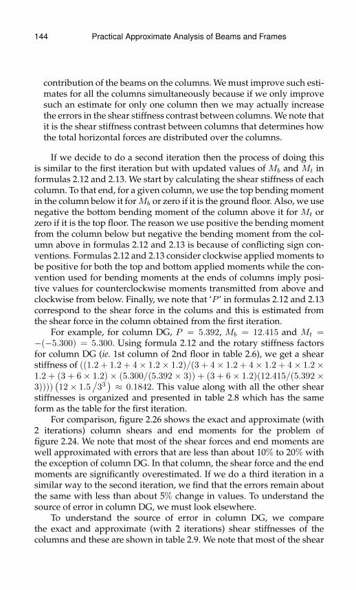
144 Practical Approximate Analysis of Beams and Frames
contribution of the beams on the columns. We must improve such esti-mates for all the columns simultaneously because if we only improvesuch an estimate for only one column then we may actually increasethe errors in the shear stiffness contrast between columns. We note thatit is the shear stiffness contrast between columns that determines howthe total horizontal forces are distributed over the columns.
If we decide to do a second iteration then the process of doing thisis similar to the first iteration but with updated values of Mb and Mt informulas 2.12 and 2.13. We start by calculating the shear stiffness of eachcolumn. To that end, for a given column, we use the top bending momentin the column below it forMb or zero if it is the ground floor. Also, we usenegative the bottom bending moment of the column above it for Mt orzero if it is the top floor. The reason we use positive the bending momentfrom the column below but negative the bending moment from the col-umn above in formulas 2.12 and 2.13 is because of conflicting sign con-ventions. Formulas 2.12 and 2.13 consider clockwise applied moments tobe positive for both the top and bottom applied moments while the con-vention used for bending moments at the ends of columns imply posi-tive values for counterclockwise moments transmitted from above andclockwise from below. Finally, we note that ‘P ’ in formulas 2.12 and 2.13correspond to the shear force in the colums and this is estimated fromthe shear force in the column obtained from the first iteration.
For example, for column DG, P = 5.392, Mb = 12.415 and Mt =−(−5.300) = 5.300. Using formula 2.12 and the rotary stiffness factorsfor column DG (ie. 1st column of 2nd floor in table 2.6), we get a shearstiffness of ((1.2 + 1.2 + 4× 1.2× 1.2)/(3 + 4× 1.2 + 4× 1.2 + 4× 1.2×1.2 + (3 + 6 × 1.2) × (5.300/(5.392 × 3)) + (3 + 6 × 1.2)(12.415/(5.392 ×3))))
(12× 1.5
/33)≈ 0.1842. This value along with all the other shear
stiffnesses is organized and presented in table 2.8 which has the sameform as the table for the first iteration.
For comparison, figure 2.26 shows the exact and approximate (with2 iterations) column shears and end moments for the problem offigure 2.24. We note that most of the shear forces and end moments arewell approximated with errors that are less than about 10% to 20% withthe exception of column DG. In that column, the shear force and the endmoments are significantly overestimated. If we do a third iteration in asimilar way to the second iteration, we find that the errors remain aboutthe same with less than about 5% change in values. To understand thesource of error in column DG, we must look elsewhere.
To understand the source of error in column DG, we comparethe exact and approximate (with 2 iterations) shear stiffnesses of thecolumns and these are shown in table 2.9. We note that most of the shear

Practical Approximate Analysis of Beams and Frames 145
Table 2.8. Second Iteration Calculations of Shear Stiffness, Shear Force and EndMoments in the Columns Shown in Figure 2.24.
Iteration number = 1
Floor = 1column number 1 2 3shear stiffness 0.209 0.060 0.271 0.540relative shear stiffness 0.387 0.111 0.503 1shear 6.960 1.994 9.046 18Internal moment at top 10.125 7.977 15.790Internal moment at bottom −17.713 0 −20.395
Floor = 2column number 1 2 3shear stiffness 0.184 0.296 0.079 0.559relative shear stiffness 0.329 0.529 0.141 1shear 4.611 7.413 1.976 14Internal moment at top 7.962 10.251 5.929Internal moment at bottom −5.869 −11.988 0
Floor = 3column number 1 2 3shear stiffness 0.180 0.046 0.182 0.409relative shear stiffness 0.441 0.113 0.447 1shear 3.525 0.903 3.572 8Internal moment at top 6.166 0 5.659Internal moment at bottom −4.408 −2.708 −5.058
Table 2.9. Comparison Between the Exact and Approximate (2 Iteration) ShearStiffness of the Columns Shown in Figure 2.24.
shear stiffness column 1 column 2 column 3exact (approx) exact (approx) exact (approx)
floor 1 0.207 (0.209) 0.062 (0.060) 0.261 (0.271)floor 2 0.111 (0.184) 0.333 (0.296) 0.081 (0.079)floor 3 0.126 (0.180) 0.032 (0.046) 0.160 (0.182)
stiffnesses are very well estimated with the biggest exception being col-umn DG (ie. column 1 and floor 2). If then consider figure 2.26 and theway in which we have estimated the rotary stiffness of the beams, we canthen account for most of this discrepancy. In particular, we have consid-ered beam GH as providing 1.5 times its rotary stiffness to column DGbut since it has an internal hinge at end H, it can only provide 0.75 timesits rotary stiffness. Therefore, the shear stiffness should be much lowerthan the standard but simple to apply estimate that we have used inthese calculations.
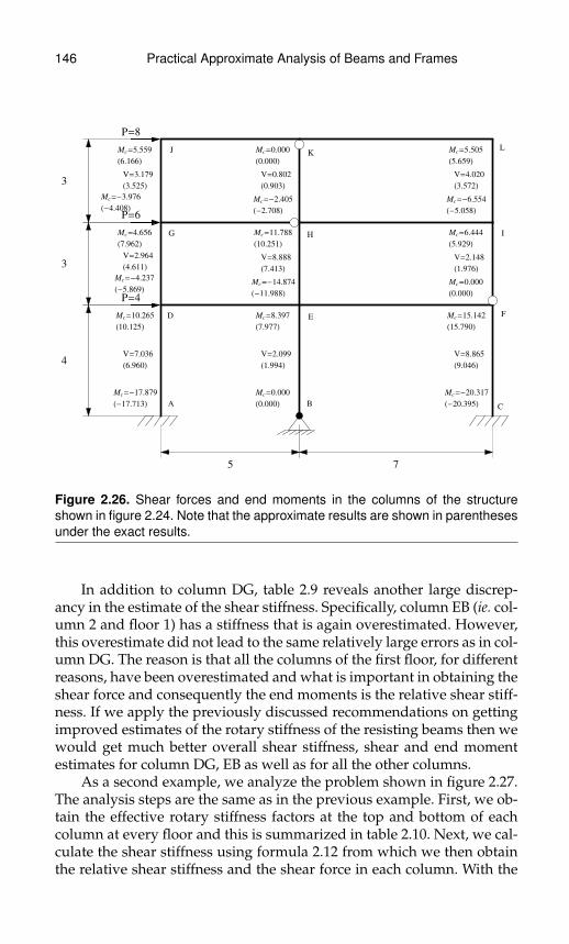
146 Practical Approximate Analysis of Beams and Frames
5 7
4
3
3
P=4
P=6
P=8
A BC
D EF
G H I
JK
L
V=7.036
H6.960L
V=2.964
H4.611L
V=3.179
H3.525L
V=2.099
H1.994L
V=8.888
H7.413L
V=0.802
H0.903L
V=8.865
H9.046L
V=2.148
H1.976L
V=4.020
H3.572L
Mc=-17.879
H-17.713L
Mc=10.265
H10.125L
Mc=-4.237
H-5.869L
Mc=4.656
H7.962L
Mc=-3.976
H-4.408L
Mc=5.559
H6.166L
Mc=0.000
H0.000L
Mc=8.397
H7.977L
Mc=-14.874
H-11.988L
Mc=11.788
H10.251L
Mc=-2.405
H-2.708L
Mc=0.000
H0.000L
Mc=-20.317
H-20.395L
Mc=15.142
H15.790L
Mc=0.000
H0.000L
Mc=6.444
H5.929L
Mc=-6.554
H-5.058L
Mc=5.505
H5.659L
Figure 2.26. Shear forces and end moments in the columns of the structureshown in figure 2.24. Note that the approximate results are shown in parenthesesunder the exact results.
In addition to column DG, table 2.9 reveals another large discrep-ancy in the estimate of the shear stiffness. Specifically, column EB (ie. col-umn 2 and floor 1) has a stiffness that is again overestimated. However,this overestimate did not lead to the same relatively large errors as in col-umn DG. The reason is that all the columns of the first floor, for differentreasons, have been overestimated and what is important in obtaining theshear force and consequently the end moments is the relative shear stiff-ness. If we apply the previously discussed recommendations on gettingimproved estimates of the rotary stiffness of the resisting beams then wewould get much better overall shear stiffness, shear and end momentestimates for column DG, EB as well as for all the other columns.
As a second example, we analyze the problem shown in figure 2.27.The analysis steps are the same as in the previous example. First, we ob-tain the effective rotary stiffness factors at the top and bottom of eachcolumn at every floor and this is summarized in table 2.10. Next, we cal-culate the shear stiffness using formula 2.12 from which we then obtainthe relative shear stiffness and the shear force in each column. With the
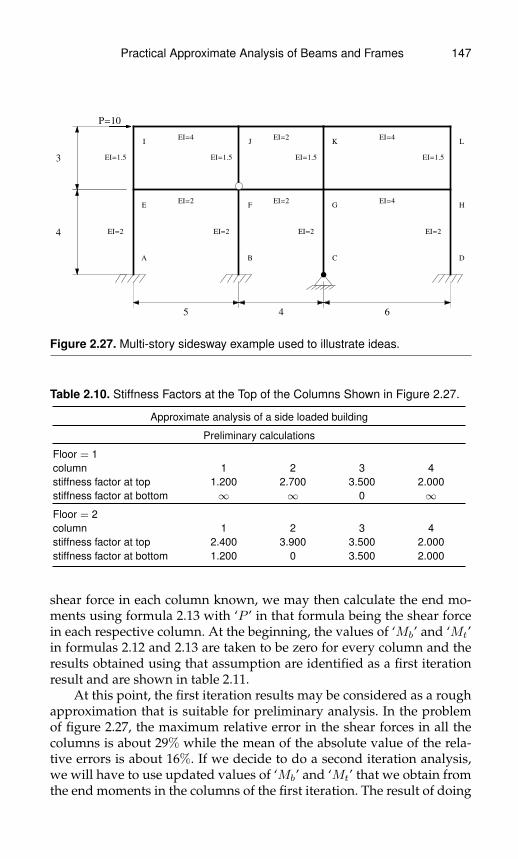
Practical Approximate Analysis of Beams and Frames 147
5 4 6
4
3
EI=2
EI=4
EI=2
EI=2
EI=4
EI=4
EI=2
EI=1.5
EI=2
EI=1.5
EI=2
EI=1.5
EI=2
EI=1.5
P=10
A B C D
E F G H
I J K L
Figure 2.27. Multi-story sidesway example used to illustrate ideas.
Table 2.10. Stiffness Factors at the Top of the Columns Shown in Figure 2.27.
Approximate analysis of a side loaded building
Preliminary calculations
Floor = 1column 1 2 3 4stiffness factor at top 1.200 2.700 3.500 2.000stiffness factor at bottom ∞ ∞ 0 ∞
Floor = 2column 1 2 3 4stiffness factor at top 2.400 3.900 3.500 2.000stiffness factor at bottom 1.200 0 3.500 2.000
shear force in each column known, we may then calculate the end mo-ments using formula 2.13 with ‘P ’ in that formula being the shear forcein each respective column. At the beginning, the values of ‘Mb’ and ‘Mt’in formulas 2.12 and 2.13 are taken to be zero for every column and theresults obtained using that assumption are identified as a first iterationresult and are shown in table 2.11.
At this point, the first iteration results may be considered as a roughapproximation that is suitable for preliminary analysis. In the problemof figure 2.27, the maximum relative error in the shear forces in all thecolumns is about 29% while the mean of the absolute value of the rela-tive errors is about 16%. If we decide to do a second iteration analysis,we will have to use updated values of ‘Mb’ and ‘Mt’ that we obtain fromthe end moments in the columns of the first iteration. The result of doing

148 Practical Approximate Analysis of Beams and Frames
Table 2.11. First Iteration Calculations of Shear Stiffness, Shear Force and EndMoments in the Columns Shown in Figure 2.27.
Iteration number = 1
Floor = 1column number 1 2 3 4shear stiffness 0.247 0.299 0.077 0.281 0.905relative shear stiffness 0.273 0.331 0.085 0.311 1shear 2.732 3.305 0.853 3.109 10Internal moment at top 4.522 6.050 3.414 5.527Internal moment at bottom −6.407 −7.171 0 −6.909
Floor = 2column number 1 2 3 4shear stiffness 0.349 0.140 0.467 0.381 1.336relative shear stiffness 0.261 0.105 0.349 0.285 1shear 2.609 1.046 3.493 2.852 10Internal moment at top 4.224 3.139 5.240 4.277Internal moment at bottom −3.603 0 −5.240 −4.277
Table 2.12. Second Iteration Calculations of Shear Stiffness, Shear Force andEnd Moments in the Columns Shown in Figure 2.27.
Iteration number = 2
Floor = 1column number 1 2 3 4shear stiffness 0.202 0.299 0.061 0.240 0.802relative shear stiffness 0.252 0.373 0.076 0.299 1shear 2.518 3.730 0.758 2.994 10Internal moment at top 3.546 6.828 3.032 4.848Internal moment at bottom −6.525 −8.093 0 −7.129
Floor = 2column number 1 2 3 4shear stiffness 0.259 0.140 0.425 0.298 1.122relative shear stiffness 0.231 0.125 0.379 0.266 1shear 2.305 1.246 3.789 2.659 10Internal moment at top 4.450 3.738 5.897 4.542Internal moment at bottom −2.466 0 −5.471 −3.436
a second calculation is shown in table 2.12 and are compared with the ex-act results in figure 2.28. By doing this second iteration, we find that themaximum relative error in the shear force in all the columns is about 14%(ie. a 15% improvement in the column shears) and the mean of the abso-lute value of the relative errors is about 6% (ie. about 10% improvementfrom the first iteration).

Practical Approximate Analysis of Beams and Frames 149
5 4 6
4
3
P=10
A B C D
E F G H
I J K L
V=2.462
H2.518L
V=2.024
H2.305L
V=3.878
H3.730L
V=1.378
H1.246L
V=0.773
H0.758L
V=4.084
H3.789L
V=2.887
H2.994L
V=2.514
H2.659L
Mc=-6.398
H-6.525L
Mc=3.451
H3.546L
Mc=-2.111
H-2.466L
Mc=3.960
H4.450L
Mc=-8.285
H-8.093L
Mc=7.226
H6.828L
Mc=0.000
H0.000L
Mc=4.135
H3.738L
Mc=0.000
H0.000L
Mc=3.091
H3.032L
Mc=-6.064
H-5.471L
Mc=6.188
H5.897L
Mc=-6.965
H-7.129L
Mc=4.585
H4.848L
Mc=-3.169
H-3.436L
Mc=4.374
H4.542L
Figure 2.28. Shear forces and end moments in the columns of the structureshown in figure 2.27. Note that the approximate results are shown in parenthesesunder the exact results.
Table 2.13. Comparison Between the Exact and Approximate (2 Iteration) ShearStiffness of the Columns Shown in Figure 2.27.
shear stiffness column 1 column 2 column 3 column 4exact (approx) exact (approx) exact (approx) exact (approx)
floor 1 0.198 (0.202) 0.311 (0.299) 0.062 (0.061) 0.232 (0.240)floor 2 0.222 (0.259) 0.151 (0.140) 0.449 (0.425) 0276 (0.298)
In order to identify the main source of the error in the problem offigure 2.27, we again compare the exact versus (second iteration) ap-proximate shear stiffness of the columns. This comparison is shown intable 2.13. The results indicate that the maximum error in the shear forceand in the shear stiffness correspond to the same column. In order to im-prove the results obtained, we will find that a third iteration will not beeffective. If we do a third iteration for the problem of figure 2.27, we willget a maximum relative error in the shear forces in all the columns ofabout 15% (a slight improvement of 1% over the second iteration) and amean of the absolute value of the relative errors of about 8% (a 2% wors-ening over the second iteration). In fact, these iterations appear to con-verge but not to the exact results unless we input better estimates of theeffective rotary stiffness provided by the beams to the columns. We notethat if we use the recommendations identified previously, the biggestchange in the effective rotary stiffness would be precisely in the columnswith the largest errors. By improving our estimates of the rotary stiffness
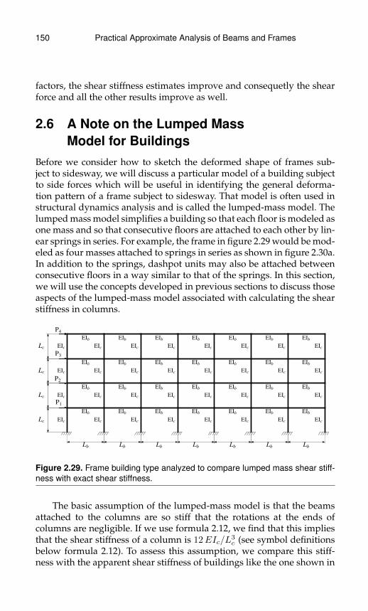
150 Practical Approximate Analysis of Beams and Frames
factors, the shear stiffness estimates improve and consequetly the shearforce and all the other results improve as well.
2.6 A Note on the Lumped MassModel for Buildings
Before we consider how to sketch the deformed shape of frames sub-ject to sidesway, we will discuss a particular model of a building subjectto side forces which will be useful in identifying the general deforma-tion pattern of a frame subject to sidesway. That model is often used instructural dynamics analysis and is called the lumped-mass model. Thelumped mass model simplifies a building so that each floor is modeled asone mass and so that consecutive floors are attached to each other by lin-ear springs in series. For example, the frame in figure 2.29 would be mod-eled as four masses attached to springs in series as shown in figure 2.30a.In addition to the springs, dashpot units may also be attached betweenconsecutive floors in a way similar to that of the springs. In this section,we will use the concepts developed in previous sections to discuss thoseaspects of the lumped-mass model associated with calculating the shearstiffness in columns.
Lb Lb Lb Lb Lb Lb Lb
Lc
Lc
Lc
Lc
EIb
EIb
EIb
EIb
EIb
EIb
EIb
EIb
EIb
EIb
EIb
EIb
EIb
EIb
EIb
EIb
EIb
EIb
EIb
EIb
EIb
EIb
EIb
EIb
EIb
EIb
EIb
EIb
EIc
EIc
EIc
EIc
EIc
EIc
EIc
EIc
EIc
EIc
EIc
EIc
EIc
EIc
EIc
EIc
EIc
EIc
EIc
EIc
EIc
EIc
EIc
EIc
EIc
EIc
EIc
EIc
EIc
EIc
EIc
EIc
P1
P2
P3
P4
Figure 2.29. Frame building type analyzed to compare lumped mass shear stiff-ness with exact shear stiffness.
The basic assumption of the lumped-mass model is that the beamsattached to the columns are so stiff that the rotations at the ends ofcolumns are negligible. If we use formula 2.12, we find that this impliesthat the shear stiffness of a column is 12EIc/L
3c (see symbol definitions
below formula 2.12). To assess this assumption, we compare this stiff-ness with the apparent shear stiffness of buildings like the one shown in

Practical Approximate Analysis of Beams and Frames 151
m1
k1
P1
m2
k2
P2
m3
k3
P3
m4
k4
P4
(a) (b) (c)
Figure 2.30. Lumped-mass system for a framed building with the first two modesof deformation assuming all columns have the same stiffness.
figure 2.29 having all its beams similar to each other and all its columnsimilar to each other and with exactly seven beam spans but with a vari-able number of floors and with a variable ratio of the beam to columnrotary stiffness (ie. (EIc/Lc) / (EIb/Lb)).
When we do an exact analysis, we find that, unlike the mass model,the shear stiffness of the columns depend on the pattern of applied sideforces ’Pi.’ The reason is that the shear stiffness of a column also de-pends on the moments transmitted from the columns above and belowit (see figure 2.19 and 2.20) which in turn depends on the pattern of ap-plied side forces. In order to decide on what pattern of side forces ismost relevant for analysis, we need to consider how we typically usethe lumped-mass model in structural dynamics. In structural dynamics,after we obtain the parameters of the lumped-mass model, we usuallydo a modal analysis. This modal analysis gives the natural frequenciesof the building and for each natural frequency we obtain a pattern ofdeformation called an eigenmode. If we rank the frequencies and theireigenmodes in order of increasing frequency, the one with the lowestfrequency is called the first mode, the second the second mode and soon. For example, the first and second modes of the lumped-mass modelshown in figure 2.30a are shown in figures 2.30b and c for some typicalconfigurational parameters.
In many buildings, it is often considered sufficiently accurate toconsider relatively few eigenmodes when doing a structural dynamicsstudy. Therefore, to test the assumptions of the lumped-mass model, we
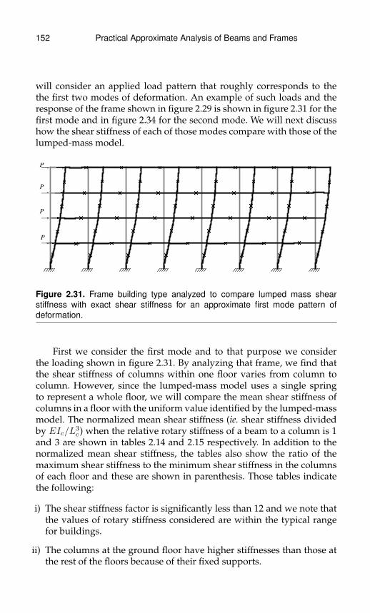
152 Practical Approximate Analysis of Beams and Frames
will consider an applied load pattern that roughly corresponds to thethe first two modes of deformation. An example of such loads and theresponse of the frame shown in figure 2.29 is shown in figure 2.31 for thefirst mode and in figure 2.34 for the second mode. We will next discusshow the shear stiffness of each of those modes compare with those of thelumped-mass model.
P
P
P
P
Figure 2.31. Frame building type analyzed to compare lumped mass shearstiffness with exact shear stiffness for an approximate first mode pattern ofdeformation.
First we consider the first mode and to that purpose we considerthe loading shown in figure 2.31. By analyzing that frame, we find thatthe shear stiffness of columns within one floor varies from column tocolumn. However, since the lumped-mass model uses a single springto represent a whole floor, we will compare the mean shear stiffness ofcolumns in a floor with the uniform value identified by the lumped-massmodel. The normalized mean shear stiffness (ie. shear stiffness dividedby EIc/L3
c) when the relative rotary stiffness of a beam to a column is 1and 3 are shown in tables 2.14 and 2.15 respectively. In addition to thenormalized mean shear stiffness, the tables also show the ratio of themaximum shear stiffness to the minimum shear stiffness in the columnsof each floor and these are shown in parenthesis. Those tables indicatethe following:
i) The shear stiffness factor is significantly less than 12 and we note thatthe values of rotary stiffness considered are within the typical rangefor buildings.
ii) The columns at the ground floor have higher stiffnesses than those atthe rest of the floors because of their fixed supports.
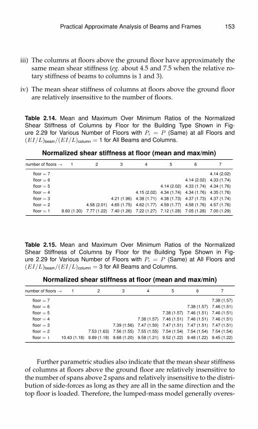
Practical Approximate Analysis of Beams and Frames 153
iii) The columns at floors above the ground floor have approximately thesame mean shear stiffness (eg. about 4.5 and 7.5 when the relative ro-tary stiffness of beams to columns is 1 and 3).
iv) The mean shear stiffness of columns at floors above the ground floorare relatively insensitive to the number of floors.
Table 2.14. Mean and Maximum Over Minimum Ratios of the NormalizedShear Stiffness of Columns by Floor for the Building Type Shown in Fig-ure 2.29 for Various Number of Floors with Pi = P (Same) at all Floors and(EI/L)beam/(EI/L)column = 1 for All Beams and Columns.
Normalized shear stiffness at floor (mean and max/min)
number of floors→ 1 2 3 4 5 6 7
floor = 7 4.14 (2.02)floor = 6 4.14 (2.02) 4.33 (1.74)floor = 5 4.14 (2.02) 4.33 (1.74) 4.34 (1.76)floor = 4 4.15 (2.02) 4.34 (1.74) 4.34 (1.76) 4.35 (1.76)floor = 3 4.21 (1.96) 4.38 (1.71) 4.38 (1.73) 4.37 (1.73) 4.37 (1.74)floor = 2 4.58 (2.01) 4.65 (1.75) 4.62 (1.77) 4.59 (1.77) 4.58 (1.76) 4.57 (1.76)floor = 1 8.60 (1.30) 7.77 (1.22) 7.40 (1.26) 7.22 (1.27) 7.12 (1.28) 7.05 (1.28) 7.00 (1.29)
Table 2.15. Mean and Maximum Over Minimum Ratios of the NormalizedShear Stiffness of Columns by Floor for the Building Type Shown in Fig-ure 2.29 for Various Number of Floors with Pi = P (Same) at All Floors and(EI/L)beam/(EI/L)column = 3 for All Beams and Columns.
Normalized shear stiffness at floor (mean and max/min)
number of floors→ 1 2 3 4 5 6 7
floor = 7 7.38 (1.57)floor = 6 7.38 (1.57) 7.46 (1.51)floor = 5 7.38 (1.57) 7.46 (1.51) 7.46 (1.51)floor = 4 7.38 (1.57) 7.46 (1.51) 7.46 (1.51) 7.46 (1.51)floor = 3 7.39 (1.56) 7.47 (1.50) 7.47 (1.51) 7.47 (1.51) 7.47 (1.51)floor = 2 7.53 (1.63) 7.56 (1.55) 7.55 (1.55) 7.54 (1.54) 7.54 (1.54) 7.54 (1.54)floor = 1 10.43 (1.18) 9.89 (1.18) 9.68 (1.20) 9.58 (1.21) 9.52 (1.22) 9.48 (1.22) 9.45 (1.22)
Further parametric studies also indicate that the mean shear stiffnessof columns at floors above the ground floor are relatively insensitive tothe number of spans above 2 spans and relatively insensitive to the distri-bution of side-forces as long as they are all in the same direction and thetop floor is loaded. Therefore, the lumped-mass model generally overes-
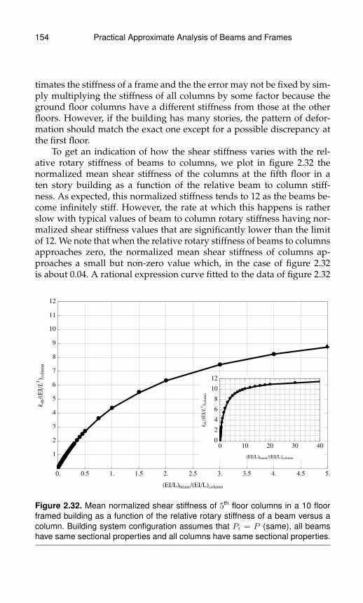
154 Practical Approximate Analysis of Beams and Frames
timates the stiffness of a frame and the the error may not be fixed by sim-ply multiplying the stiffness of all columns by some factor because theground floor columns have a different stiffness from those at the otherfloors. However, if the building has many stories, the pattern of defor-mation should match the exact one except for a possible discrepancy atthe first floor.
To get an indication of how the shear stiffness varies with the rel-ative rotary stiffness of beams to columns, we plot in figure 2.32 thenormalized mean shear stiffness of the columns at the fifth floor in aten story building as a function of the relative beam to column stiff-ness. As expected, this normalized stiffness tends to 12 as the beams be-come infinitely stiff. However, the rate at which this happens is ratherslow with typical values of beam to column rotary stiffness having nor-malized shear stiffness values that are significantly lower than the limitof 12. We note that when the relative rotary stiffness of beams to columnsapproaches zero, the normalized mean shear stiffness of columns ap-proaches a small but non-zero value which, in the case of figure 2.32is about 0.04. A rational expression curve fitted to the data of figure 2.32
æææææææææææææææææææææææææææææ
æ
æ
æ
æ
æ
æ
æ
0. 0.5 1. 1.5 2. 2.5 3. 3.5 4. 4.5 5.
1
2
3
4
5
6
7
8
9
10
11
12
HEI�LLbeam�HEI�LLcolumn
ksh�H
EI�
L3L c
olu
mn
æææææææææææææææææææææææææææææ
æ
æ
æ
æ
æ
ææææææææ æ
æ æ ææ æ
0 10 20 30 400
2
4
6
8
10
12
HEI�LLbeam�HEI�LLcolumn
ksh�H
EI�
L3L c
olu
mn
Figure 2.32. Mean normalized shear stiffness of 5th floor columns in a 10 floorframed building as a function of the relative rotary stiffness of a beam versus acolumn. Building system configuration assumes that Pi = P (same), all beamshave same sectional properties and all columns have same sectional properties.
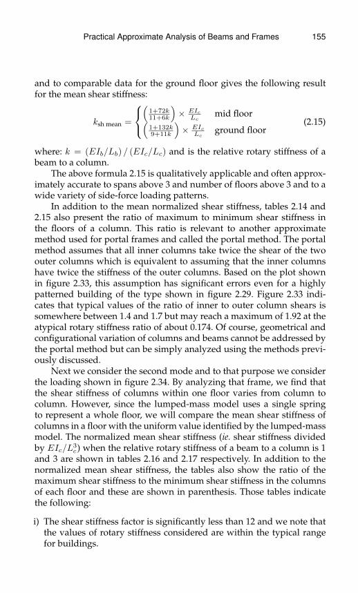
Practical Approximate Analysis of Beams and Frames 155
and to comparable data for the ground floor gives the following resultfor the mean shear stiffness:
ksh mean =
(
1+72k11+6k
)× EIc
Lcmid floor(
1+132k9+11k
)× EIc
Lcground floor
(2.15)
where: k = (EIb/Lb) / (EIc/Lc) and is the relative rotary stiffness of abeam to a column.
The above formula 2.15 is qualitatively applicable and often approx-imately accurate to spans above 3 and number of floors above 3 and to awide variety of side-force loading patterns.
In addition to the mean normalized shear stiffness, tables 2.14 and2.15 also present the ratio of maximum to minimum shear stiffness inthe floors of a column. This ratio is relevant to another approximatemethod used for portal frames and called the portal method. The portalmethod assumes that all inner columns take twice the shear of the twoouter columns which is equivalent to assuming that the inner columnshave twice the stiffness of the outer columns. Based on the plot shownin figure 2.33, this assumption has significant errors even for a highlypatterned building of the type shown in figure 2.29. Figure 2.33 indi-cates that typical values of the ratio of inner to outer column shears issomewhere between 1.4 and 1.7 but may reach a maximum of 1.92 at theatypical rotary stiffness ratio of about 0.174. Of course, geometrical andconfigurational variation of columns and beams cannot be addressed bythe portal method but can be simply analyzed using the methods previ-ously discussed.
Next we consider the second mode and to that purpose we considerthe loading shown in figure 2.34. By analyzing that frame, we find thatthe shear stiffness of columns within one floor varies from column tocolumn. However, since the lumped-mass model uses a single springto represent a whole floor, we will compare the mean shear stiffness ofcolumns in a floor with the uniform value identified by the lumped-massmodel. The normalized mean shear stiffness (ie. shear stiffness dividedby EIc/L3
c) when the relative rotary stiffness of a beam to a column is 1and 3 are shown in tables 2.16 and 2.17 respectively. In addition to thenormalized mean shear stiffness, the tables also show the ratio of themaximum shear stiffness to the minimum shear stiffness in the columnsof each floor and these are shown in parenthesis. Those tables indicatethe following:
i) The shear stiffness factor is significantly less than 12 and we note thatthe values of rotary stiffness considered are within the typical rangefor buildings.

156 Practical Approximate Analysis of Beams and Frames
æ
æ
æ
æ
æ
ææææææææææææææææææææææææ
æ
æ
æ
æ
æ
æ
æ
0. 0.5 1. 1.5 2. 2.5 3. 3.5 4. 4.5 5.0.
0.2
0.4
0.6
0.8
1.
1.2
1.4
1.6
1.8
2.
HEI�LLbeam�HEI�LLcolumn
ksh
max�k
sh
min
æ
æ
æ
ææææææææææææææææææææææææææææ
ææææææææ æ æ æ æ æ
æ æ
0 10 20 30 400.0
0.5
1.0
1.5
2.0
HEI�LLbeam�HEI�LLcolumn
ksh
max�k
sh
min
Figure 2.33. Maximum over minimum ratios of the shear stiffness of 5th floorcolumns in a 10 floor framed building as a function of the relative rotary stiffnessof a beam versus a column. Building system configuration assumes that Pi = P(same), all beams have same sectional properties and all columns have samesectional properties.
1.5 P
0.3 P
P
1.6 P
Figure 2.34. Frame building type analyzed to compare lumped mass shear stiff-ness with exact shear stiffness for second mode.
ii) The columns at the ground floor have higher stiffness than those atthe rest of the floors because of their fixed supports. In one case, whenwe have only two floors, the normalized mean shear stiffness of thecolumns at the ground floor exceeds 12 and will be explained below.
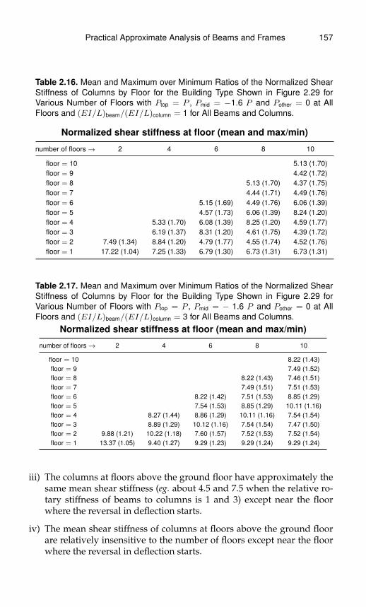
Practical Approximate Analysis of Beams and Frames 157
Table 2.16. Mean and Maximum over Minimum Ratios of the Normalized ShearStiffness of Columns by Floor for the Building Type Shown in Figure 2.29 forVarious Number of Floors with Ptop = P , Pmid = −1.6 P and Pother = 0 at AllFloors and (EI/L)beam/(EI/L)column = 1 for All Beams and Columns.
Normalized shear stiffness at floor (mean and max/min)
number of floors→ 2 4 6 8 10
floor = 10 5.13 (1.70)floor = 9 4.42 (1.72)floor = 8 5.13 (1.70) 4.37 (1.75)floor = 7 4.44 (1.71) 4.49 (1.76)floor = 6 5.15 (1.69) 4.49 (1.76) 6.06 (1.39)floor = 5 4.57 (1.73) 6.06 (1.39) 8.24 (1.20)floor = 4 5.33 (1.70) 6.08 (1.39) 8.25 (1.20) 4.59 (1.77)floor = 3 6.19 (1.37) 8.31 (1.20) 4.61 (1.75) 4.39 (1.72)floor = 2 7.49 (1.34) 8.84 (1.20) 4.79 (1.77) 4.55 (1.74) 4.52 (1.76)floor = 1 17.22 (1.04) 7.25 (1.33) 6.79 (1.30) 6.73 (1.31) 6.73 (1.31)
Table 2.17. Mean and Maximum over Minimum Ratios of the Normalized ShearStiffness of Columns by Floor for the Building Type Shown in Figure 2.29 forVarious Number of Floors with Ptop = P , Pmid = − 1.6 P and Pother = 0 at AllFloors and (EI/L)beam/(EI/L)column = 3 for All Beams and Columns.
Normalized shear stiffness at floor (mean and max/min)
number of floors→ 2 4 6 8 10
floor = 10 8.22 (1.43)floor = 9 7.49 (1.52)floor = 8 8.22 (1.43) 7.46 (1.51)floor = 7 7.49 (1.51) 7.51 (1.53)floor = 6 8.22 (1.42) 7.51 (1.53) 8.85 (1.29)floor = 5 7.54 (1.53) 8.85 (1.29) 10.11 (1.16)floor = 4 8.27 (1.44) 8.86 (1.29) 10.11 (1.16) 7.54 (1.54)floor = 3 8.89 (1.29) 10.12 (1.16) 7.54 (1.54) 7.47 (1.50)floor = 2 9.88 (1.21) 10.22 (1.18) 7.60 (1.57) 7.52 (1.53) 7.52 (1.54)floor = 1 13.37 (1.05) 9.40 (1.27) 9.29 (1.23) 9.29 (1.24) 9.29 (1.24)
iii) The columns at floors above the ground floor have approximately thesame mean shear stiffness (eg. about 4.5 and 7.5 when the relative ro-tary stiffness of beams to columns is 1 and 3) except near the floorwhere the reversal in deflection starts.
iv) The mean shear stiffness of columns at floors above the ground floorare relatively insensitive to the number of floors except near the floorwhere the reversal in deflection starts.
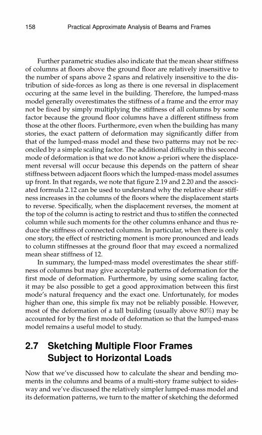
158 Practical Approximate Analysis of Beams and Frames
Further parametric studies also indicate that the mean shear stiffnessof columns at floors above the ground floor are relatively insensitive tothe number of spans above 2 spans and relatively insensitive to the dis-tribution of side-forces as long as there is one reversal in displacementoccuring at the same level in the building. Therefore, the lumped-massmodel generally overestimates the stiffness of a frame and the error maynot be fixed by simply multiplying the stiffness of all columns by somefactor because the ground floor columns have a different stiffness fromthose at the other floors. Furthermore, even when the building has manystories, the exact pattern of deformation may significantly differ fromthat of the lumped-mass model and these two patterns may not be rec-onciled by a simple scaling factor. The additional difficulty in this secondmode of deformation is that we do not know a-priori where the displace-ment reversal will occur because this depends on the pattern of shearstiffness between adjacent floors which the lumped-mass model assumesup front. In that regards, we note that figure 2.19 and 2.20 and the associ-ated formula 2.12 can be used to understand why the relative shear stiff-ness increases in the columns of the floors where the displacement startsto reverse. Specifically, when the displacement reverses, the moment atthe top of the column is acting to restrict and thus to stiffen the connectedcolumn while such moments for the other columns enhance and thus re-duce the stiffness of connected columns. In particular, when there is onlyone story, the effect of restricting moment is more pronounced and leadsto column stiffnesses at the ground floor that may exceed a normalizedmean shear stiffness of 12.
In summary, the lumped-mass model overestimates the shear stiff-ness of columns but may give acceptable patterns of deformation for thefirst mode of deformation. Furthermore, by using some scaling factor,it may be also possible to get a good approximation between this firstmode’s natural frequency and the exact one. Unfortunately, for modeshigher than one, this simple fix may not be reliably possible. However,most of the deformation of a tall building (usually above 80%) may beaccounted for by the first mode of deformation so that the lumped-massmodel remains a useful model to study.
2.7 Sketching Multiple Floor FramesSubject to Horizontal Loads
Now that we’ve discussed how to calculate the shear and bending mo-ments in the columns and beams of a multi-story frame subject to sides-way and we’ve discussed the relatively simpler lumped-mass model andits deformation patterns, we turn to the matter of sketching the deformed
Practical Approximate Analysis of Beams and Frames 159
shape of frames subject to sidesway. In this regards, we will extend theprocedure developed for sketching single floor portal frames. The stepsremain the same and these are repeated concisely below:
i) Draw the column and beam chords.
ii) Draw the directions or tangents to most columns and beams at thenodes or connections.
iii) Draw the columns by using the tangents at the nodes and fig-ures 2.14 and 2.15 as a guide for the ground floor and figure 2.20for the other floors.
iv) Draw the beams by using the tangents at the nodes as a guide.
v) Draw the column or columns with rollers (if any) using the tangentsas a guide and knowing that those columns must be subject to arigid rotation.
vi) Remove extraneous lines that were used in constructing the sketchin order to get a better looking drawing of the deformed shape. Inthis step, we recommend that the chords be kept because they helpto clarify the deformations of the columns and beams.
In the above steps, we will give additional suggestions on how tosketch the chords of columns and the deformed columns themselves.This is additional information related to steps (i) and (iii) above. The restof the steps are similar to sketching the previously discussed single floorportal.
We start by discussing how to sketch the column chords. In a singlefloor portal, we simply choose a convenient slope for the chord of anycolumn and all the other chords of the columns must be parallel to thatone. This observation still applies on a floor by floor basis in a multi-storyframe. Once we choose the sidesway or slope of one of the chords of thecolumns in a given floor then all the other chords of the columns on thesame floor must be parallel to that one. What remains to be discussed isthe relative slopes of the chords at different floors. In that regards, wewill find it useful to define a frame’s chord-line to be the line joininga representative chord of a column from each floor connected to otherrepresentative columns in successive floors all the way from the groundto the top floor.
The shape of a frame’s chord-line depends on how the total shearstiffness of all columns in a floor vary from floor to floor and on the pat-tern of side loading. To estimate this shape, we can use the lumped-massmodel with the shear stiffness of the columns adjusted according to the
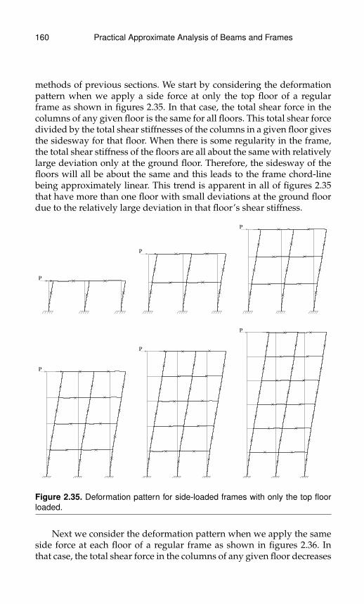
160 Practical Approximate Analysis of Beams and Frames
methods of previous sections. We start by considering the deformationpattern when we apply a side force at only the top floor of a regularframe as shown in figures 2.35. In that case, the total shear force in thecolumns of any given floor is the same for all floors. This total shear forcedivided by the total shear stiffnesses of the columns in a given floor givesthe sidesway for that floor. When there is some regularity in the frame,the total shear stiffness of the floors are all about the same with relativelylarge deviation only at the ground floor. Therefore, the sidesway of thefloors will all be about the same and this leads to the frame chord-linebeing approximately linear. This trend is apparent in all of figures 2.35that have more than one floor with small deviations at the ground floordue to the relatively large deviation in that floor’s shear stiffness.
P
P
P
P
P
P
Figure 2.35. Deformation pattern for side-loaded frames with only the top floorloaded.
Next we consider the deformation pattern when we apply the sameside force at each floor of a regular frame as shown in figures 2.36. Inthat case, the total shear force in the columns of any given floor decreases

Practical Approximate Analysis of Beams and Frames 161
P P
P
P
P
P
P
P
P
P
P
P
P
P
P
P
P
P
P
P
P
Figure 2.36. Deformation pattern for side-loaded frames with a uniform distribu-tion of loads per floor.
linearly from the ground floor where this total shear force equals the totalof all side forces on the ground floor until the top floor where this totalshear force equals only the side force applied at the top floor. As before,when there is some regularity in the frame, the total shear stiffness ofthe floors are all about the same with relatively large deviation only atthe ground floor. Therefore, the sidesway of the floors will vary in anapproximately linear manner and this leads to the frame chord-line beingapproximately parabolic. This trend is apparent in all of figures 2.36 thathave more than two floors with small deviations at the ground floor dueto the relatively large deviation in that floor’s shear stiffness.
Next we consider the deformation pattern when we only apply aside force at the top floor but there is a discontinuity in shear stiffness inone of the floors as shown in figures 2.37 and 2.38. The discontinuity infigure 2.37 is due to placing internal hinges at the top of all the columnsof one of the floors which significantly reduces the shear stiffness of that
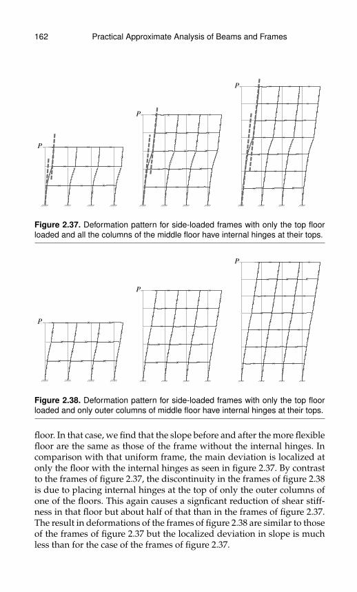
162 Practical Approximate Analysis of Beams and Frames
P
P
P
Figure 2.37. Deformation pattern for side-loaded frames with only the top floorloaded and all the columns of the middle floor have internal hinges at their tops.
P
P
P
Figure 2.38. Deformation pattern for side-loaded frames with only the top floorloaded and only outer columns of middle floor have internal hinges at their tops.
floor. In that case, we find that the slope before and after the more flexiblefloor are the same as those of the frame without the internal hinges. Incomparison with that uniform frame, the main deviation is localized atonly the floor with the internal hinges as seen in figure 2.37. By contrastto the frames of figure 2.37, the discontinuity in the frames of figure 2.38is due to placing internal hinges at the top of only the outer columns ofone of the floors. This again causes a signficant reduction of shear stiff-ness in that floor but about half of that than in the frames of figure 2.37.The result in deformations of the frames of figure 2.38 are similar to thoseof the frames of figure 2.37 but the localized deviation in slope is muchless than for the case of the frames of figure 2.37.
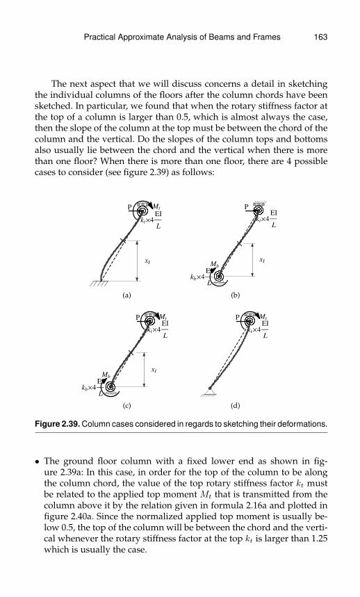
Practical Approximate Analysis of Beams and Frames 163
The next aspect that we will discuss concerns a detail in sketchingthe individual columns of the floors after the column chords have beensketched. In particular, we found that when the rotary stiffness factor atthe top of a column is larger than 0.5, which is almost always the case,then the slope of the column at the top must be between the chord of thecolumn and the vertical. Do the slopes of the column tops and bottomsalso usually lie between the chord and the vertical when there is morethan one floor? When there is more than one floor, there are 4 possiblecases to consider (see figure 2.39) as follows:
kt´4EI
L
MtP
xI
(a)
kb´4EI
L
Mb
kt´4EI
L
P
xI
(b)
kb´4EI
L
Mb
kt´4EI
L
MtP
xI
(c)
kt´4EI
L
MtP
(d)
Figure 2.39. Column cases considered in regards to sketching their deformations.
• The ground floor column with a fixed lower end as shown in fig-ure 2.39a: In this case, in order for the top of the column to be alongthe column chord, the value of the top rotary stiffness factor kt mustbe related to the applied top moment Mt that is transmitted from thecolumn above it by the relation given in formula 2.16a and plotted infigure 2.40a. Since the normalized applied top moment is usually be-low 0.5, the top of the column will be between the chord and the verti-cal whenever the rotary stiffness factor at the top kt is larger than 1.25which is usually the case.

164 Practical Approximate Analysis of Beams and Frames
0. 0.1 0.2 0.3 0.4 0.5 0.6 0.7 0.8 0.9 1.0.
0.2
0.4
0.6
0.8
1.
1.2
1.4
1.6
1.8
2.
Mt�PL
kt
Combinations where top slope tangent to chord
Case: Mb=0, kb®¥
(a)
kt=1
kt=2
kt=4
kt=¥
0. 0.1 0.2 0.3 0.4 0.5 0.6 0.7 0.8 0.9 1.0.
0.2
0.4
0.6
0.8
1.
1.2
1.4
1.6
1.8
2.
Mb�PL
kb
Combinations where lower slope tangent to chord
Case: Mt=0
(b)
Figure 2.40. Conditions where a column’s slope is tangent to the chord for thecases of figure 2.39a, b and c. Figure 2.39d never has the column line tangentto its chord. For figure 2.39c only the special case when Mb = Mt is shown.(Continued below.)
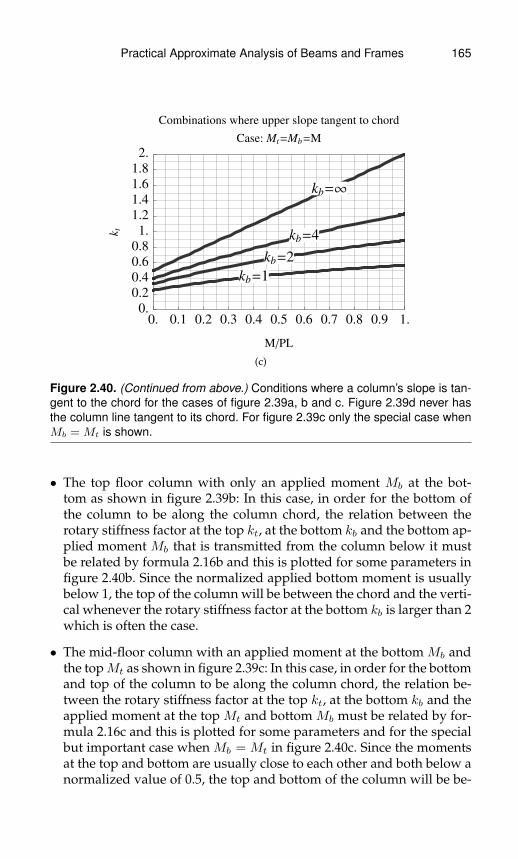
Practical Approximate Analysis of Beams and Frames 165
kb=1
kb=2
kb=4
kb=¥
0. 0.1 0.2 0.3 0.4 0.5 0.6 0.7 0.8 0.9 1.0.
0.2
0.4
0.6
0.8
1.
1.2
1.4
1.6
1.8
2.
M�PL
kt
Combinations where upper slope tangent to chord
Case: Mt=Mb=M
(c)
Figure 2.40. (Continued from above.) Conditions where a column’s slope is tan-gent to the chord for the cases of figure 2.39a, b and c. Figure 2.39d never hasthe column line tangent to its chord. For figure 2.39c only the special case whenMb = Mt is shown.
• The top floor column with only an applied moment Mb at the bot-tom as shown in figure 2.39b: In this case, in order for the bottom ofthe column to be along the column chord, the relation between therotary stiffness factor at the top kt, at the bottom kb and the bottom ap-plied moment Mb that is transmitted from the column below it mustbe related by formula 2.16b and this is plotted for some parameters infigure 2.40b. Since the normalized applied bottom moment is usuallybelow 1, the top of the column will be between the chord and the verti-cal whenever the rotary stiffness factor at the bottom kb is larger than 2which is often the case.
• The mid-floor column with an applied moment at the bottom Mb andthe topMt as shown in figure 2.39c: In this case, in order for the bottomand top of the column to be along the column chord, the relation be-tween the rotary stiffness factor at the top kt, at the bottom kb and theapplied moment at the top Mt and bottom Mb must be related by for-mula 2.16c and this is plotted for some parameters and for the specialbut important case when Mb = Mt in figure 2.40c. Since the momentsat the top and bottom are usually close to each other and both below anormalized value of 0.5, the top and bottom of the column will be be-
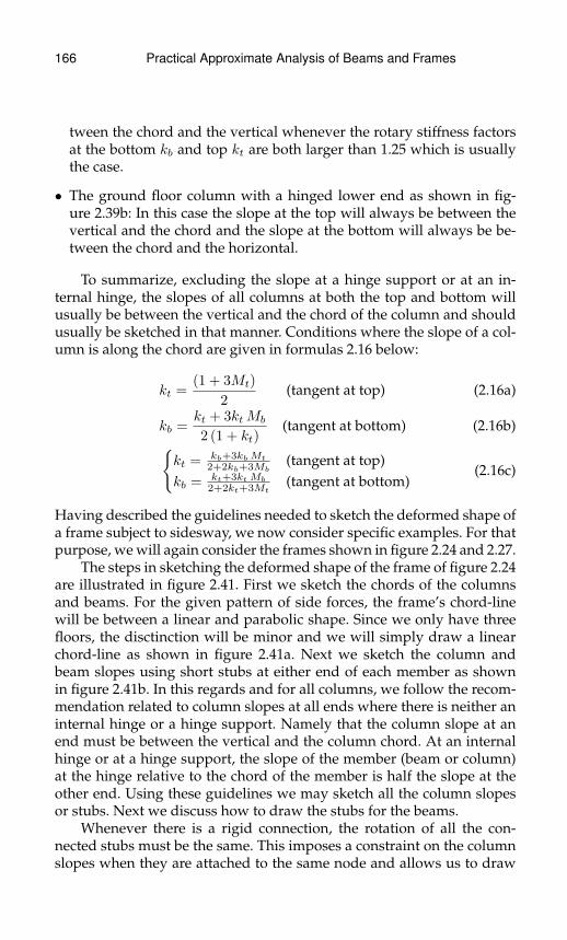
166 Practical Approximate Analysis of Beams and Frames
tween the chord and the vertical whenever the rotary stiffness factorsat the bottom kb and top kt are both larger than 1.25 which is usuallythe case.
• The ground floor column with a hinged lower end as shown in fig-ure 2.39b: In this case the slope at the top will always be between thevertical and the chord and the slope at the bottom will always be be-tween the chord and the horizontal.
To summarize, excluding the slope at a hinge support or at an in-ternal hinge, the slopes of all columns at both the top and bottom willusually be between the vertical and the chord of the column and shouldusually be sketched in that manner. Conditions where the slope of a col-umn is along the chord are given in formulas 2.16 below:
kt =(1 + 3Mt)
2(tangent at top) (2.16a)
kb =kt + 3ktMb
2 (1 + kt)(tangent at bottom) (2.16b){
kt = kb+3kbMt
2+2kb+3Mb(tangent at top)
kb = kt+3ktMb
2+2kt+3Mt(tangent at bottom)
(2.16c)
Having described the guidelines needed to sketch the deformed shape ofa frame subject to sidesway, we now consider specific examples. For thatpurpose, we will again consider the frames shown in figure 2.24 and 2.27.
The steps in sketching the deformed shape of the frame of figure 2.24are illustrated in figure 2.41. First we sketch the chords of the columnsand beams. For the given pattern of side forces, the frame’s chord-linewill be between a linear and parabolic shape. Since we only have threefloors, the disctinction will be minor and we will simply draw a linearchord-line as shown in figure 2.41a. Next we sketch the column andbeam slopes using short stubs at either end of each member as shownin figure 2.41b. In this regards and for all columns, we follow the recom-mendation related to column slopes at all ends where there is neither aninternal hinge or a hinge support. Namely that the column slope at anend must be between the vertical and the column chord. At an internalhinge or at a hinge support, the slope of the member (beam or column)at the hinge relative to the chord of the member is half the slope at theother end. Using these guidelines we may sketch all the column slopesor stubs. Next we discuss how to draw the stubs for the beams.
Whenever there is a rigid connection, the rotation of all the con-nected stubs must be the same. This imposes a constraint on the columnslopes when they are attached to the same node and allows us to draw

Practical Approximate Analysis of Beams and Frames 167
A B C
D E F
G HI
JK
L
(a)
A B C
D E F
G HI
JK
L
(b)
A B C
D E F
G HI
JK
L
(c)
A B C
D E F
G HI
JK
L
(d)
Figure 2.41. Steps in sketching the deformed shape of problem 2.24.
stubs at the ends of all beams where there is a rigid connection. At beamends that are connected to a node where all the attached columns havean internal hinge at that connection (for example node K in figure 2.41),the rotation of the beams at the connection is dictated by the beam rota-tions at the other ends of those beams. In this regards, we need to use themethods related to sketching the deformation of beams with no sides-way because the beams of each floor behave as shown in figure 2.11.
Once the stubs at all beam and column endings have been sketched,we then sketch the column lines. These follow the same guidelines asthose for the single floor portal and is shown in figure 2.41c. Finally, thedeformed shape of all beams are sketched using the methods of beamswith no sidesway and this is shown in figure 2.41d. By removing extrane-ous lines including the stubs constructed in figure 2.41b, we get a cleanerlooking sketch of the deformed frame and this is shown in figure 2.42.
The steps in sketching the deformed shape of the frame of figure 2.27are illustrated in figure 2.43. These are similar to the previous case. Firstwe sketch the column chords as shown in figure 2.43a. Second, we sketchstubs indicating the slopes at the ends of all columns and beams. Unlikethe previous example, in this case the rotation of all beams are dictatedby the rotation of the columns and the result is shown in figure 2.43b.

168 Practical Approximate Analysis of Beams and Frames
P=4
P=6
P=8
A
B C
D E F
G HI
JK
L
Figure 2.42. Sketch of deformed shape of problem 2.24.
A B C D
E F GH
I J K L
(a)
A B C D
E F GH
I J K L
(b)
A B C D
E F GH
I J K L
(c)
A B C D
E F GH
I J K L
(d)
Figure 2.43. Steps in sketching the deformed shape of problem 2.27.
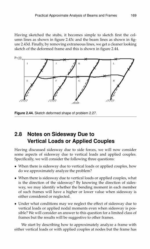
Practical Approximate Analysis of Beams and Frames 169
Having sketched the stubs, it becomes simple to sketch first the col-umn lines as shown in figure 2.43c and the beam lines as shown in fig-ure 2.43d. Finally, by removing extraneous lines, we get a cleaner lookingsketch of the deformed frame and this is shown in figure 2.44.
P=10
A B C D
E F G H
I J K L
Figure 2.44. Sketch deformed shape of problem 2.27.
2.8 Notes on Sidesway Due toVertical Loads or Applied Couples
Having discussed sidesway due to side forces, we will now considersome aspects of sidesway due to vertical loads and applied couples.Specifically, we will consider the following three questions:
• When there is sidesway due to vertical loads or applied couples, howdo we approximately analyze the problem?
• When there is sidesway due to vertical loads or applied couples, whatis the direction of the sidesway? By knowing the direction of sides-way, we may identify whether the bending moment in each memberof such frames will have a higher or lower value when sidesway iseither considered or neglected.
• Under what conditions may we neglect the effect of sidesway due tovertical loads or applied nodal moments even when sidesway is pos-sible? We will consider an answer to this question for a limited class offrames but the results will be suggestive to other frames.
We start by describing how to approximately analyze a frame witheither vertical loads or with applied couples at nodes but the frame has
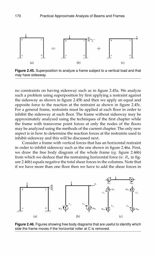
170 Practical Approximate Analysis of Beams and Frames
A
B C
D
(a)
=A
B C
D
Rx
(b)
+A
B C
D
Rx
(c)
Figure 2.45. Superposition to analyze a frame subject to a vertical load and thatmay have sidesway.
no constraints on having sidesway such as in figure 2.45a. We analyzesuch a problem using superposition by first applying a restraint againstthe sidesway as shown in figure 2.45b and then we apply an equal andopposite force to the reaction at the restraint as shown in figure 2.45c.For a general frame, restraints must be applied at each floor in order toinhibit the sidesway at each floor. The frame without sidesway may beapproximately analyzed using the techniques of the first chapter whilethe frame with transverse point forces at only the nodes of the floorsmay be analyzed using the methods of the current chapter. The only newaspect is in how to determine the reaction forces at the restraints used toinhibit sidesway and this will be discussed next.
Consider a frame with vertical forces that has an horizontal restraintin order to inhibit sidesway such as the one shown in figure 2.46a. First,we draw the free body diagram of the whole frame (eg. figure 2.46b)from which we deduce that the restraining horizontal force (ie. Rx in fig-ure 2.46b) equals negative the total shear forces in the columns. Note thatif we have more than one floor then we have to add the shear forces in
A
B C
D
(a)
FLx
Rx
FRx
MLBMRB
(b)
FLx
FLx
MLB
MLT
MLT MRT
FRx
FRx
MRB
MRT
(c)
Figure 2.46. Figures showing free body diagrams that are useful to identify whichside the frame moves if the horizontal roller at C is removed.
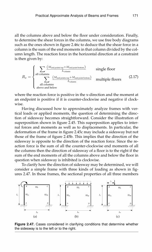
Practical Approximate Analysis of Beams and Frames 171
all the columns above and below the floor under consideration. Finally,to determine the shear forces in the columns, we use free body diagramssuch as the ones shown in figure 2.46c to deduce that the shear force in acolumn is the sum of the end moments in that column divided by the col-umn length. The reaction force in the horizontal direction at a constraintis then given by:
Rx =
∑all columns
(Mend points top+Mend point bottom)Lcolumn
single floor∑all columns
above and below
(Mend points top+Mend point bottom)Lcolumn
multiple floors(2.17)
where the reaction force is positive in the x-direction and the moment atan endpoint is positive if it is counter-clockwise and negative if clock-wise.
Having discussed how to approximately analyze frames with ver-tical loads or applied moments, the question of determining the direc-tion of sidesway becomes straightforward. Consider the illustration ofsuperposition shown in figure 2.45. This superposition applies to inter-nal forces and moments as well as to displacements. In particular, thedeformation of the frame in figure 2.45c may include a sidesway but notthose of the frame of figure 2.45b. This implies that the direction of thesidesway is opposite to the direction of the reaction force. Since the re-action force is the sum of all the counter-clockwise end moments of allthe columns then the direction of sidesway of a floor is to the right if thesum of the end moments of all the columns above and below the floor inquestion when sidesway is inhibited is clockwise.
To clarify how the direction of sidesway may be determined, we willconsider a simple frame with three kinds of loading as shown in fig-ures 2.47. In those frames, the sectional properties of all three members
EIcLLc
EIb
Lb
EIcR
A
B C
D
(a)
EIcLLc
EIb
Lb
EIcR
A
B C
D
(b)
EIcLLc
EIb
Lb
EIcR
A
B C
D
xF
(c)
Figure 2.47. Cases considered in clarifying conditions that determine whetherthe sidesway is to the left or to the right.

172 Practical Approximate Analysis of Beams and Frames
may be different and the length of the columns and the beam may beindependently chosen. In addition, for figure 2.47c, the location of thepoint force may vary across the beam. As a reference, we give the exactresult for the sidesway in those frames which is as follows:
∆ =
(kL−kR)16z
LcL3b
EIbq uniform load
(2kL−kR+2kLkR)4z
LcLb
EIbMapp applied moment
(1− xF ) xF
×(
(2kL−kR+2kLkR)4z
− (kL+kR+4kLkR)xF
4z
)LcL
2b
EIbP
point force(2.18)
where:
z = 3kL + k2L + 3kR + 11kLkR + k2LkR + k2R + kLk2R
kL = (EIcL/Lc) / (EIb/Lb)
kR = (EIcR/Lc) / (EIb/Lb)
‘q’ is the magnitude of the uniform load
‘Mapp’ is the magnitude of the applied moment
‘P ’ is the magnitude of the point force
x = xF/Lb where xF is the distance of the point force from the left end
In all the cases considered in figure 2.47, we note the following:
• In all cases, the top end moments of the left column are clockwise andthose of the top right column are counter-clocwise.
• In all cases, the bottom end moments of a column are half the top onesand are of the same sign.
Therefore, in all cases, if the top end moment on the left column ishigher than the corresponding one on the right column then the sides-way will be to the right and it will be to the left otherwise. We next con-sider each of the three cases separately.
First we consider the frame in figure 2.47a with a clockwise appliedmoment. For the three cases considered in figure 2.48, we note the fol-lowing:
• The applied moment is distributed on the beam and on the left columnin proportion to their rotary stiffness which is approximately propor-tional to the sectional property ‘EI’ where ‘E’ is Young’s modulus and‘I’ is the moment of inertia.
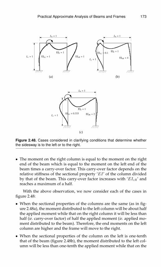
Practical Approximate Analysis of Beams and Frames 173
EIcL = 1Lc = 1
EIb = 1
Lb = 1
EIcR = 1
(a)
EIcL = 0.1
Lc = 1
EIb = 1
Lb = 1
EIcR = 4
(b)
EIcL = 0.333Lc = 1
EIb = 1
Lb = 1
EIcR = 2
(c)
Figure 2.48. Cases considered in clarifying conditions that determine whetherthe sidesway is to the left or to the right.
• The moment on the right column is equal to the moment on the rightend of the beam which is equal to the moment on the left end of thebeam times a carry-over factor. This carry-over factor depends on therelative stiffness of the sectional property ‘EI’ of the column dividedby that of the beam. This carry-over factor increases with ‘EIcR’ andreaches a maximum of a half.
With the above observation, we now consider each of the cases infigure 2.48:
• When the sectional properties of the columns are the same (as in fig-ure 2.48a), the moment distributed to the left column will be about halfthe applied moment while that on the right column it will be less thanhalf (ie. carry-over factor) of half the applied moment (ie. applied mo-ment distributed to the beam). Therefore, the end moments on the leftcolumn are higher and the frame will move to the right.
• When the sectional properties of the column on the left is one-tenththat of the beam (figure 2.48b), the moment distributed to the left col-umn will be less than one-tenth the applied moment while that on the

174 Practical Approximate Analysis of Beams and Frames
right column will be close to half of nine-tenth the applied moment.Therefore, the end moments on the right column are higher and theframe will move to the left.
• When the sectional properties of the column are as is shown in fig-ure 2.48c, an approximate analysis of the frame with sidesway inhib-ited gives end moments in the columns that are about the same. There-fore, sidesway will be zero or negligible.
Next we consider the frame in figure 2.47b. For the three cases con-sidered in figure 2.49, we note the following:
• The moments at the ends of the beam equal the moments at the top ofthe columns.
• The moments at the ends of the beam are related to the rotary stiffnessfactors at the ends. In particular, the end with the higher rotary stiff-ness factor will have a higher end moment. This means that the endwith a higher value of ‘EI’ will have a higher end moment becausethe length of the columns are identical.
With the above observation, we now consider each of the cases infigure 2.49:
EIcL = 1Lc = 1EIb = 1
Lb = 1
q
EIcR = 1
(a)
EIcL = 4Lc = 1EIb = 1
Lb = 1
q
EIcR = 1
(b)
EIcL = 1Lc = 1EIb = 1
Lb = 1
q
EIcR = 4
(c)
Figure 2.49. Cases considered in clarifying conditions that determine whetherthe sidesway is to the left or to the right.

Practical Approximate Analysis of Beams and Frames 175
• When the sectional properties of the columns are the same as in fig-ure 2.49a then the end moments on the columns are the same andthere is no sidesway. Note that, in this case, we could also have de-duced this fact based on the simultaneous symmetry of the geometry,material and loading.
• When the rotary stiffness of the left column is higher as in figure 2.49bthen the sidesway is to the right and when this is lower as in fig-ure 2.49c then the sidesway is to the left.
Next we consider the frame in figure 2.47c with an applied pointforce. For the six cases considered in figure 2.50, we note the following:
• The moments at the ends of the beam equal the moments at the top ofthe columns.
• The moments at the ends of the beam are related to the rotary stiffnessfactors at the ends. In particular, the end moment at an end increaseswith the rotary stiffness factor at that end.
• The moments at the ends of the beam are also related to the location ofthe point force. In particular, for the same material properties, as thepoint force approaches an end, the moment at that end will tend toincrease relative to the other end.
• The above observations taken together imply that there are two com-peting effects, the location of the point force and the relative rotarystiffness factors of the columns.
With the above observation, we now consider each of the cases infigure 2.50:
• When the sectional properties of the columns are the same and thepoint force is at the middle of the beam as in figure 2.50a then theend moments on the columns are the same and there is no sidesway.Note that, in this case, we could also have deduced this based on thesimultaneous symmetry of the geometry, material and loading.
• When the sectional properties of the columns are the same and thepoint force is closer to the left end of the beam as in figure 2.50b thenthe end moments on the left columns are higher and sidesway is to theright. This is because the rotary stiffness factor does not favor any sidein terms of higher internal moments but the point force favors the leftside column.
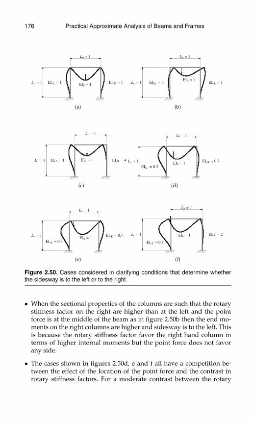
176 Practical Approximate Analysis of Beams and Frames
EIcL = 1Lc = 1EIb = 1
Lb = 1
EIcR = 1
(a)
EIcL = 1Lc = 1EIb = 1
Lb = 1
EIcR = 1
(b)
EIcL = 1Lc = 1 EIb = 1
Lb = 1
EIcR = 4
(c)
EIcL = 0.3
Lc = 1EIb = 1
Lb = 1
EIcR = 0.7
(d)
EIcL = 0.3
Lc = 1EIb = 1
Lb = 1
EIcR = 0.7
(e)
EIcL = 0.3
Lc = 1 EIb = 1
Lb = 1
EIcR = 2
(f)
Figure 2.50. Cases considered in clarifying conditions that determine whetherthe sidesway is to the left or to the right.
• When the sectional properties of the columns are such that the rotarystiffness factor on the right are higher than at the left and the pointforce is at the middle of the beam as in figure 2.50b then the end mo-ments on the right columns are higher and sidesway is to the left. Thisis because the rotary stiffness factor favor the right hand column interms of higher internal moments but the point force does not favorany side.
• The cases shown in figures 2.50d, e and f all have a competition be-tween the effect of the location of the point force and the contrast inrotary stiffness factors. For a moderate contrast between the rotary

Practical Approximate Analysis of Beams and Frames 177
stiffness factors of the columns, the sidesway is to the left when thepoint force is not sufficiently close to the left end as in figure 2.50dand it is to the right when it gets sufficiently close to the left end as infigure 2.50e. However, when the stiffness contrast between the rotarystiffness factors of the columns is above a threshold as in figure 2.50fthen the effect of the location of the point force will always be weakerthan the effect of rotary stiffness contrast and the frame will alwayshave a sidesway to the left.
Finally, we consider the question of whether we can neglect the ef-fect of sidesway due to vertical loads or applied nodal moments evenwhen sidesway is possible. In order to study this question, we considera single floor but multi-bay portal frame subject to either an applied mo-ment at the leftmost end as in figures 2.51, or to an applied uniform loadon the leftmost beam as in figure 2.52, or to an applied point force onthe leftmost beam as in figure 2.54. In each case, we consider the internalmoment at the left end of the leftmost beam when the sidesway is inhib-ited as in figures 2.51a, 2.52a and 2.54a and when sidesway is allowedas in figures 2.51b, b and b. The reason we consider the internal momentat the left end of the leftmost beam is that this is usually the largest (orclose to the largest) internal moment in the frame.
LbLb
Lc
LbLb
EIc EIc
EIb
EIc EIc EIcEIc
EIb EIbEIb
︸ ︷︷ ︸(a) variable number of bays or spans
LbLb
Lc
LbLb
EIc EIc
EIb
EIc EIc EIcEIc
EIb EIbEIb
︸ ︷︷ ︸(b) variable number of bays or spans
Figure 2.51. A single floor regular portal frame with variable number of bayssubject to a point moment at only the leftmost node.
LbLb
Lc
LbLb
EIc EIc
EIb
EIc EIc EIcEIc
EIb EIbEIb
︸ ︷︷ ︸(a) variable number of bays or spans
LbLb
Lc
LbLb
EIc EIc
EIb
EIc EIc EIcEIc
EIb EIbEIb
︸ ︷︷ ︸(b) variable number of bays or spans
Figure 2.52. A single floor regular portal frame with variable number of bayssubject to a uniform load on only the leftmost span.

178 Practical Approximate Analysis of Beams and Frames
2 3 4 5 6 7 8 9 10 11 12 13 14 15
-10
0
10
20
30
number of bays
Err
or%
Max error Hwith vs without sideswayL
Applied moment
(a)
2 3 4 5 6 7 8 9 10 11 12 13 14 15
-20
-15
-10
-5
0
number of bays
Err
or%
Max error Hwith vs without sideswayL
Uniform distributed load
(b) variable number of bays or spans
Figure 2.53. Percent error between the leftmost moments of the leftmost beamswhen the sidesway is neglected or when it is included versus the number ofbays or spans. Figure 2.53a is for an applied moment at the leftmost node andfigure 2.53b is for an applied uniform load on the leftmost span. In both figures,0.5 ≤ (EIc/Lc) / (EIb/Lb) ≤ 2 and 0.8 ≤ Lb/Lc ≤ 2.
First, we consider the cases of an applied moment (figures 2.51) andof an applied uniform load (figures 2.52). In those cases, there are effec-tively two parameters that affect the relative error between the abovespecified internal moment when there is and when there is no sides-way. These parameters are the relative length of a column to a beam(ie. Lb/Lc) and the relative rotary stiffness factor of a column to a beam(ie. (EIc/Lc) / (EIb/Lb)). For each configuration, we consider the largestpositive and negative errors for any value of these parameters withina range typical for those parameters (see related figure captions) andplot the error range as a function of the number of bays as shown in fig-ure 2.53a and b for the applied moment and for the uniform load casesrespectively. The results shown in the plots indicate that the error de-creases as the number of bays increases so that if we allow a maximum
LbLb
Lc
LbLb
EIc EIc
EIb
EIc EIc EIcEIc
EIb EIbEIb
xF
︸ ︷︷ ︸(a) variable number of bays or spans
LbLb
Lc
LbLb
EIc EIc
EIb
EIc EIc EIcEIc
EIb EIbEIb
xF
︸ ︷︷ ︸(b) variable number of bays or spans
Figure 2.54. A single floor regular portal frame with variable number of bayssubject to a point force on only the leftmost span.
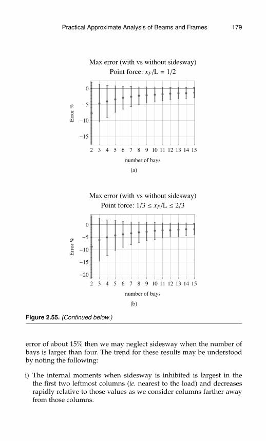
Practical Approximate Analysis of Beams and Frames 179
2 3 4 5 6 7 8 9 10 11 12 13 14 15
-15
-10
-5
0
number of bays
Err
or%
Max error Hwith vs without sideswayL
Point force: xF�L = 1�2
(a)
2 3 4 5 6 7 8 9 10 11 12 13 14 15
-20
-15
-10
-5
0
number of bays
Err
or%
Max error Hwith vs without sideswayL
Point force: 1�3 £ xF�L £ 2�3
(b)
Figure 2.55. (Continued below.)
error of about 15% then we may neglect sidesway when the number ofbays is larger than four. The trend for these results may be understoodby noting the following:
i) The internal moments when sidesway is inhibited is largest in thethe first two leftmost columns (ie. nearest to the load) and decreasesrapidly relative to those values as we consider columns farther awayfrom those columns.

180 Practical Approximate Analysis of Beams and Frames
2 3 4 5 6 7 8 9 10 11 12 13 14 15
-20
-15
-10
-5
0
number of bays
Err
or%
Max error Hwith vs without sideswayL
Point force: 1�4 £ xF�L £ 3�4
(c)
Figure 2.55. (Continued from above.) Percent error between the leftmost mo-ments of the leftmost beams when the sidesway is neglected or when it is in-cluded versus the number of bays or spans. The figures are for an applied pointforce on the leftmost beam with the location of the point force restricted to thecenter for figure 2.55a, the middle third of the span for figure 2.55b and the middlehalf of the span for figure 2.55c. In both figures, 0.5 ≤ (EIc/Lc) / (EIb/Lb) ≤ 2and 0.8 ≤ Lb/Lc ≤ 2.
ii) Negative the restraining force inhibiting sidesway will be distributedover all the columns when we superpose back the effect of the restrain-ing force in order to get the unrestrained case (eg. see figure 2.45 andrelated explanations).
The above two observations implies that the restraining force whensidesway is inhibited changes relatively little as the number of bays in-creases but negative this restraining force gets distributed over a largernumber of columns producing progressively less end moments in thosecolumns to be superposed back in order to get the unrestrained case.Hence, the error between the cases when sidesway is inhibited and whenit is not inhibited will decrease with the number of bays.
For the case when a point force is applied on the leftmost beam asin figures 2.54, we have an additional parameter which is the location ofthe point force on the beam. For each configuration specified by (Lb/Lc),(EIc/Lc) / (EIb/Lb) and (xF /Lb), we again consider the largest positiveand negative errors for any value of these parameters within a rangetypical for those parameters (see related figure captions) and plot thoseas a function of the number of bays as shown in figure 2.55a, b and c. Thecases differ in the range that is allowed for the location of the point force.

Practical Approximate Analysis of Beams and Frames 181
The results shown in the plots indicate that the error again decreases asthe number of bays increases so that if we allow a maximum error ofabout 15% then we may neglect sidesway when the number of bays isabout three for all three ranges of the location of the point force. Thetrend for these results may be understood in the same way as those forthe applied moment or applied uniform load.

This page intentionally left blank
Chapter 3
Estimating Displacementsin Beams and Frames
3.1 Maximum Vertical Displacementsin Beams
In this chapter, we will discuss deflections and rotations in beams andframes. Some of the material will overlap with previous discussions re-lated to the sketching of beams and frames but the emphasis here is oncalculating or estimating the maximum deflection or rotation. In thissection, we will graphically present deflection results in terms of stiff-ness factors. To estimate the maximum deflection in any beam that isattached to a passive structure, we first estimate the stiffness factors atthe ends and then use the appropriate plot or formula to obtain themaximum displacement. For convenience, simpler approximate formu-las are presented in this section with exact formulas being relegated tothe appendices.
We start our presentation with the case of an applied moment atan end and a passive resistance at the other as shown in figure 3.1a.In this case, the maximum deflection always occurs nearer to the endwhere the moment is applied at a distance between about 0.333 and 0.423times the length of the member and occur when the stiffness factor is 0and ∞ respectively. The value of the maximum deflection is betweenabout 0.0370 and 0.0642 times MappL
2/EI where ‘Mapp’ is the magni-tude of the applied moment, ‘L’ is the length of the beam and ‘EI’ is themoment of inertia of the beam. We note that the largest maximum deflec-tion is
√3 (≈ 1.732) times the smallest maximum deflection. The results
of both the location and value of the maximum deflection are shown in
183

184 Practical Approximate Analysis of Beams and Frames
L
k´4
EI
L
Mapp
umax
xat max
(a)
L
kR´4
EI
L
kL´4
EI
L
umax
xat max
q
(b)
L
kR´4
EI
L
kL´4
EI
L
umax
xat max
xF
P
(c)
Figure 3.1. Cases considered in calculating maximum deflections.
0.01 0.1 1 10 1000.33
0.34
0.35
0.36
0.37
0.38
0.39
0.4
0.41
0.42
k
xatm
ax�L
Location of maximum displacement
Applied end moment
(a)
0.01 0.1 1 10 1000.0
0.2
0.4
0.6
0.8
1.0
k
u`m
ax
Normalized maximum displacement H27� 3 L umax�HMappL2�EIL
Applied end moment
(b) variable number of bays or spans
Figure 3.2. Location and value of the maximum deflection for the case shown infigure 3.1a.
figures 3.2. Finally, an aproximate formula for the maximum deflection isgiven by:
umax Mapp ≈(1 + 0.8k)
(16 + 22k)
Mapp L2
EI(3.1)
We note that the above approximate formula always underestimates thedeflection and has a maximum error that is always less than 1.82% whichoccurs when k = 0.
The next case we consider is that of a uniform load with passivesupports on each side as shown in figure 3.1b. In this case the maxi-mum deflection always occurs closer to the more flexible side (ie. theside whose stiffness factor is lower) and always lies between about 0.422and 0.578 times the length of the beam. In other words, the location ofthe maximum is within about 7.84% of the length of the beam from the
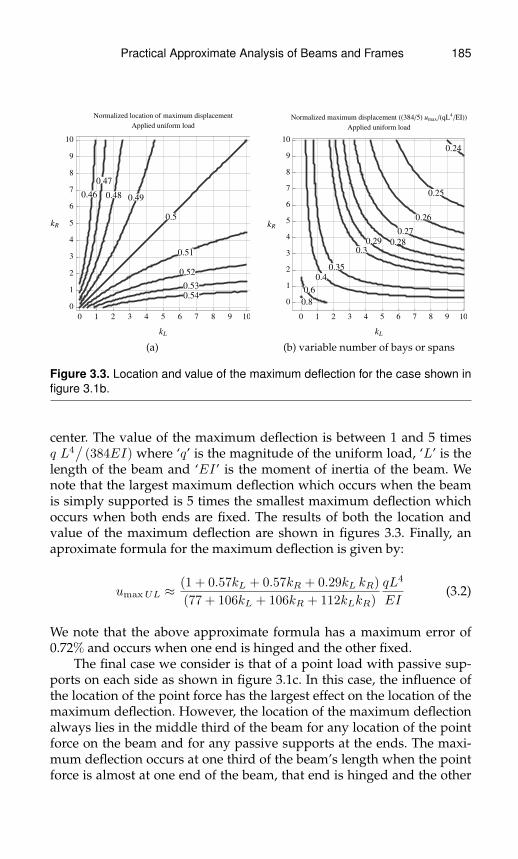
Practical Approximate Analysis of Beams and Frames 185
0.46
0.47
0.48 0.49
0.5
0.51
0.52
0.53
0.54
0 1 2 3 4 5 6 7 8 9 10
0
1
2
3
4
5
6
7
8
9
10
kL
kR
Normalized location of maximum displacement
Applied uniform load
(a)
0.24
0.25
0.26
0.27
0.280.29
0.3
0.35
0.4
0.6
0.8
0 1 2 3 4 5 6 7 8 9 10
0
1
2
3
4
5
6
7
8
9
10
kL
kR
Normalized maximum displacement HH384�5L umax�HqL4�EILL
Applied uniform load
(b) variable number of bays or spans
Figure 3.3. Location and value of the maximum deflection for the case shown infigure 3.1b.
center. The value of the maximum deflection is between 1 and 5 timesq L4
/(384EI) where ‘q’ is the magnitude of the uniform load, ‘L’ is the
length of the beam and ‘EI’ is the moment of inertia of the beam. Wenote that the largest maximum deflection which occurs when the beamis simply supported is 5 times the smallest maximum deflection whichoccurs when both ends are fixed. The results of both the location andvalue of the maximum deflection are shown in figures 3.3. Finally, anaproximate formula for the maximum deflection is given by:
umaxUL ≈(1 + 0.57kL + 0.57kR + 0.29kL kR)
(77 + 106kL + 106kR + 112kLkR)
qL4
EI(3.2)
We note that the above approximate formula has a maximum error of0.72% and occurs when one end is hinged and the other fixed.
The final case we consider is that of a point load with passive sup-ports on each side as shown in figure 3.1c. In this case, the influence ofthe location of the point force has the largest effect on the location of themaximum deflection. However, the location of the maximum deflectionalways lies in the middle third of the beam for any location of the pointforce on the beam and for any passive supports at the ends. The maxi-mum deflection occurs at one third of the beam’s length when the pointforce is almost at one end of the beam, that end is hinged and the other
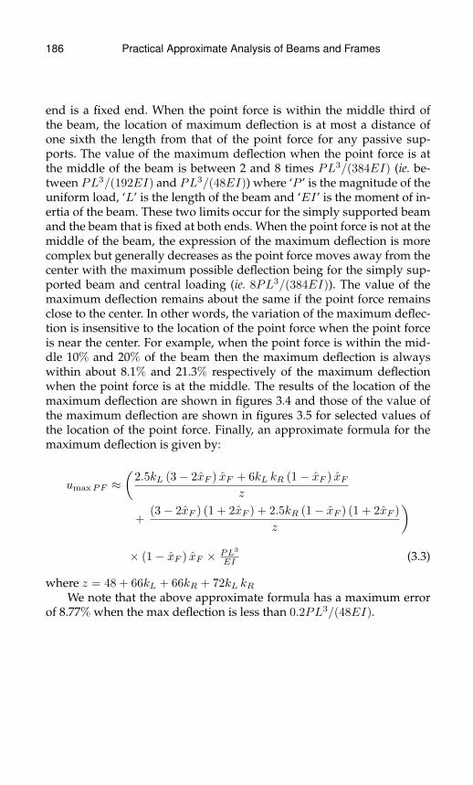
186 Practical Approximate Analysis of Beams and Frames
end is a fixed end. When the point force is within the middle third ofthe beam, the location of maximum deflection is at most a distance ofone sixth the length from that of the point force for any passive sup-ports. The value of the maximum deflection when the point force is atthe middle of the beam is between 2 and 8 times PL3/(384EI) (ie. be-tween PL3/(192EI) and PL3/(48EI)) where ‘P ’ is the magnitude of theuniform load, ‘L’ is the length of the beam and ‘EI’ is the moment of in-ertia of the beam. These two limits occur for the simply supported beamand the beam that is fixed at both ends. When the point force is not at themiddle of the beam, the expression of the maximum deflection is morecomplex but generally decreases as the point force moves away from thecenter with the maximum possible deflection being for the simply sup-ported beam and central loading (ie. 8PL3/(384EI)). The value of themaximum deflection remains about the same if the point force remainsclose to the center. In other words, the variation of the maximum deflec-tion is insensitive to the location of the point force when the point forceis near the center. For example, when the point force is within the mid-dle 10% and 20% of the beam then the maximum deflection is alwayswithin about 8.1% and 21.3% respectively of the maximum deflectionwhen the point force is at the middle. The results of the location of themaximum deflection are shown in figures 3.4 and those of the value ofthe maximum deflection are shown in figures 3.5 for selected values ofthe location of the point force. Finally, an approximate formula for themaximum deflection is given by:
umaxPF ≈(
2.5kL (3− 2xF ) xF + 6kL kR (1− xF ) xFz
+(3− 2xF ) (1 + 2xF ) + 2.5kR (1− xF ) (1 + 2xF )
z
)× (1− xF ) xF × PL3
EI(3.3)
where z = 48 + 66kL + 66kR + 72kL kRWe note that the above approximate formula has a maximum error
of 8.77% when the max deflection is less than 0.2PL3/(48EI).
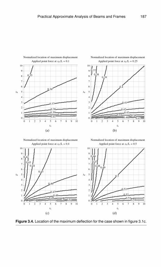
Practical Approximate Analysis of Beams and Frames 187
0.35
0.36
0.37
0.38
0.390.4
0.41
0 1 2 3 4 5 6 7 8 9 10
0
1
2
3
4
5
6
7
8
9
10
kL
kR
Normalized location of maximum displacement
Applied point force at xF�L = 0.1
(a)
0.37
0.38
0.39
0.4
0.41
0.42
0.43
0.440.45
0.46 0.47
0 1 2 3 4 5 6 7 8 9 10
0
1
2
3
4
5
6
7
8
9
10
kL
kR
Normalized location of maximum displacement
Applied point force at xF�L = 0.25
(b)
0.42
0.43
0.44
0.45
0.46
0.47
0.48
0.490.5 0.51
0 1 2 3 4 5 6 7 8 9 10
0
1
2
3
4
5
6
7
8
9
10
kL
kR
Normalized location of maximum displacement
Applied point force at xF�L = 0.4
(c)
0.46
0.47
0.480.49
0.5
0.51
0.52
0.530.54
0 1 2 3 4 5 6 7 8 9 10
0
1
2
3
4
5
6
7
8
9
10
kL
kR
Normalized location of maximum displacement
Applied point force at xF�L = 0.5
(d)
Figure 3.4. Location of the maximum deflection for the case shown in figure 3.1c.

188 Practical Approximate Analysis of Beams and Frames
0.046
0.05
0.06
0.080.1
0.15
0.2
0 1 2 3 4 5 6 7 8 9 10
0
1
2
3
4
5
6
7
8
9
10
kL
kR
Normalized max displacement H48 umax�HPL3�EILL
Applied point force at xF�L = 0.1
(a)
0.165
0.17
0.18
0.2
0.250.3
0.4
0.6
0 1 2 3 4 5 6 7 8 9 10
0
1
2
3
4
5
6
7
8
9
10
kL
kR
Normalized max displacement H48 umax�HPL3�EILL
Applied point force at xF�L = 0.25
(b)
0.27
0.28
0.3
0.35
0.4
0.50.6
0.8
0 1 2 3 4 5 6 7 8 9 10
0
1
2
3
4
5
6
7
8
9
10
kL
kR
Normalized max displacement H48 umax�HPL3�EILL
Applied point force at xF�L = 0.4
(c)
0.29
0.3
0.32
0.34
0.36
0.4
0.5
0.6
0 1 2 3 4 5 6 7 8 9 10
0
1
2
3
4
5
6
7
8
9
10
kL
kR
Normalized max displacement H48 umax�HPL3�EILL
Applied point force at xF�L = 0.5
(d)
Figure 3.5. Value of the maximum deflection for the case shown in figure 3.1c.

Practical Approximate Analysis of Beams and Frames 189
3.2 Estimating Moment of InertiaFor an actual beam, we can, with practice or experience, make a goodestimate of its dimensions simply by looking at it. Also, by being famil-iar with the concept of area and with some practice or experience, wecan also estimate areas of cross-sections by a visual inspection and someminor calculations. For example, one approach to estimate areas is tomentally rearrange the cross-section, without stretching or leaving gaps,into an equivalent rectangle whose area we then calculate based on ourestimates of dimensions. By contrast, rules to estimate the moment ofinertia are not obvious but such a skill would be useful for a structuralengineer because formulas for deflections and bending stresses promi-nently involve the moment of inertia. This is especially important inoptimization where we seek the relative advantage of different shapesboth in regards to constructability and in regards to providing the largestmoment of inertia for a given weight. In this section, we will developsome guidance in estimating moments of inertia for arbitrary sections,in quickly sorting various sectional shapes in terms of their momentsof inertia and in identifying what features in the shape most affect themoments of inertia.
We will consider shape transformations that either do not changethe moment of inertia or change it in a simple and easy to calculate man-ner. In this discussion, we will focus on the moment of inertia relativeto an horizontal axis. A similar discussion may be done for the momentof inertia relative to a vertical axis which can be easily deduced after ro-tating the page by 90◦. The first transformation we consider leaves themoment of inertia relative to an horizontal axis invariant. That transfor-mation consists of any shape change that maintains unchanged the netwidth at every horizontal cut. Note that this transformation also leavesthe area invariant. For example, consider the shapes shown in figure 3.6.By sliding the middle portions of the box section (figure 3.6a) from bothleft and right towards the center, we get the I-beam (figure 3.6b) with thenet width at each height remaining the same. Furthermore, by slidingthe middle portion of the I-beam to the far right, we get the C-channel(figure 3.6c). Therefore, we deduce that all three sections shown in fig-ures 3.6 have the same moment of inertia relative to an horizontal axis.
A special case of the transformation discussed above is that of a lin-ear sideways shearing. A uniform sideways shear leaves the net widthat each horizontal cut unchanged and therefore will also leave the mo-ment of inertia unchanged. As an example, figures 3.7 shows an isosce-les triangle (figure 3.7a) that is uniformly sheared into a right triangle(figure 3.7b) and then into an obtuse triangle (figure 3.7c). Therefore,the three triangles in figures 3.7 all have the same moment of inertia

190 Practical Approximate Analysis of Beams and Frames
b
tw�2 tw�2
t f
t f
h
(a)
b
tw
t f
t f
h
(b)
b
tw
t f
t f
h
(c)
Figure 3.6. Shapes 3.6a, b and c above all have the same area, moment of inertiaabout any horizontal axis and radius of gyration about any horizontal axis. Thesesectional properties remain the same when the net width at every horizontal cutremains the same.
h
b b b
HaL HbL HcL
Figure 3.7. Shapes 3.7a, b and c above all have the same area, moment ofinertia about any horizontal axis and radius of gyration about any horizontal axis.These sectional properties remain the same when there is uniform shearing inthe horizontal direction because such shearing leaves the net width at everyhorizontal cut invariant.
relative to an horizontal axis. Note that the characteristic of a linear side-ways shearing transformation is that straight lines are transformed intostraight lines of the same height. For example, transforming a rectangleinto a parallelogram of the same height and base also leaves the momentof inertia invariant.
The third transformation we will consider changes the value of themoment of inertia but in a simple manner. If we uniformly stretch orcontract (ie. scale) a cross-section horizontally so that the width at ev-ery horizontal cut is multiplied or divided by the same factor then boththe area and the moment of inertia will be multiplied or divided by the

Practical Approximate Analysis of Beams and Frames 191
h
b=h�2 b=h b=2h
HaL HbL HcL
A�2
I�2
Area=A
Moment of inertia=I
2A
2I
Figure 3.8. Shapes 3.8a, b and c above have area, moment of inertia about anyhorizontal axis and radius of gyration about any horizontal axis that scale withthe width. These sectional properties increase proportionately to the amount ofscaling in the horizontal direction.
same factor. As an example, we consider a disk that is either contractedor stretched by a factor of 2 as shown in figures 3.8. In that case, the thinellipse in figure 3.8a will have half the area and half the moment of inertiarelative to an horizontal axis as that of the disk in figure 3.8b. Similarly,the wide ellipse in figure 3.8c will have twice those same quantities as thedisk. We note that because this transformation scales both the moment ofinertia and the area by the same factor, then the radius of gyration whichis the square root of their ratio is invariant under this transformation. Inaddition, since the height remains the same, the ratio of the moment ofinertia divided by the maximum moment of inertia also remains invari-ant under this transformation. As will be discussed below, since this ra-tio may be used as a measure of the efficiency of a given shape, thereforean horizontal scaling does not change the efficiency of a cross-sectionalshape.
The next transformation we will consider relates the moment of in-ertia of a symmetric section with that of an unsymmetric one. We startwith a cross-section that is symmetric relative to an horizontal axis but isotherwise unconstrained as for example the cross-section shown in fig-ure 3.9a. If we now remove an arbitrary piece of this cross-section, reflectit relative to the horizontal axis of symmetry and add it to the reflectedside, we then get an unsymmetric cross-section. For example, we haveused this process to transform the cross-section of figure 3.9a into that offigure 3.9b, however, we have additionally horizontally slid the reflectedpiece in order to enhance clarity. Such a further horizontal sliding doesnot affect the moment of inertia relative to an horizontal axis because it
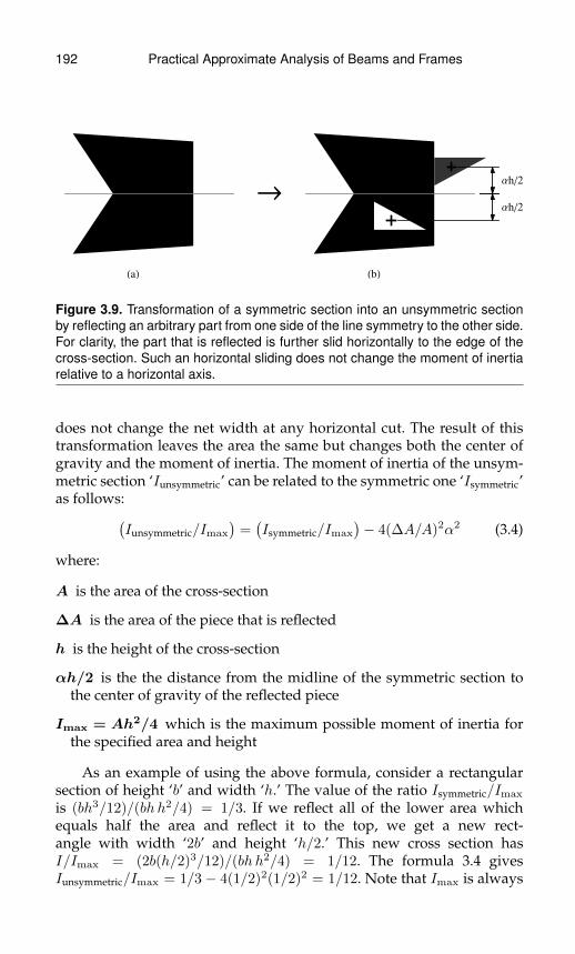
192 Practical Approximate Analysis of Beams and Frames
®Αh�2
Αh�2
HaL HbL
Figure 3.9. Transformation of a symmetric section into an unsymmetric sectionby reflecting an arbitrary part from one side of the line symmetry to the other side.For clarity, the part that is reflected is further slid horizontally to the edge of thecross-section. Such an horizontal sliding does not change the moment of inertiarelative to a horizontal axis.
does not change the net width at any horizontal cut. The result of thistransformation leaves the area the same but changes both the center ofgravity and the moment of inertia. The moment of inertia of the unsym-metric section ‘Iunsymmetric’ can be related to the symmetric one ‘Isymmetric’as follows:(
Iunsymmetric/Imax
)=(Isymmetric/Imax
)− 4(∆A/A)2α2 (3.4)
where:
A is the area of the cross-section
∆A is the area of the piece that is reflected
h is the height of the cross-section
αh/2 is the the distance from the midline of the symmetric section tothe center of gravity of the reflected piece
Imax = Ah2/4 which is the maximum possible moment of inertia forthe specified area and height
As an example of using the above formula, consider a rectangularsection of height ‘b’ and width ‘h.’ The value of the ratio Isymmetric/Imax
is (bh3/12)/(bh h2/4) = 1/3. If we reflect all of the lower area whichequals half the area and reflect it to the top, we get a new rect-angle with width ‘2b’ and height ‘h/2.’ This new cross section hasI/Imax = (2b(h/2)3/12)/(bh h2/4) = 1/12. The formula 3.4 givesIunsymmetric/Imax = 1/3− 4(1/2)2(1/2)2 = 1/12. Note that Imax is always

Practical Approximate Analysis of Beams and Frames 193
relative to the original height even if all the area on one side is beingreflected.
There are several things that are interesting in formula 3.4 which in-clude:
• The formula applies for both ∆A positive (removal then reflection ofarea) as well as negative (adding then reflecting negative area).
• Iunsymmetric is always less than Isymmetric because the difference is alwaysnegative. Note that this does not mean that all unsymmetric sectionshave lower moments of inertia than symmetric ones. However, it doesmean that if an unsymmetric section can be related to a symmetric onethrough such a transformation then the symmetric section will havea higher moment of inertia. It also means that the above describedtransformation always lowers the moment of inertia of a symmetricsection. Furthermore, the result can be used to prove that for a fixedarea and height, the maximum moment of inertia is that of the idealI-beam with all the areas being symmetrically placed at the farthestallowable locations.
• If we remove and reflect a piece from only one side then (∆A/A) ≤ 1/2and α ≤ 1. This implies that the difference between Iunsymmetric/Imax
and Isymmetric/Imax is always less or equal to one.
• The decrease in the moment of inertia is quadratic with ‘∆A/A’ andwith ‘α.’ Since these are both less than one if we are removing andreflecting area from only one side then the change in moment of inertiabetween a symmetric section and its associated unsymmetric sectionwill generally be a relatively small change. For example, if we removeand reflect at most 20% of the area from one side (ie. 10% of the totalarea) then the change in moment of inertia will be less than 24% for allshapes that are at least as efficient as a diamond shape (see table 3.2and related discussions).
To clarify the effect of this last transformation, we study two cross-sectional shapes, namely the I-beam with a negligible web width but fi-nite flange thickness and the rectangular cross-section. For the I-beam,we use formula 3.4 to plot the ratio of moment of inertia of the unsym-metric to the symmetric one versus the ratio of top to bottom flangewidth. As expected, the maximum occurs for the symmetric section andthe variation is parabolic near that maximum and this is shown in fig-ure 3.10a for (b/h)symmetric = 1 and in figure 3.10b for (b/h)symmetric = 2.Note that even when the non-symmetric I-beam has a side whose widthis twice (or half) the other side, its moment of inertia is about 92.7% and

194 Practical Approximate Analysis of Beams and Frames
0. 0.5 1. 1.5 2. 2.5 3. 3.5 4. 4.5 5.0.
0.1
0.2
0.3
0.4
0.5
0.6
0.7
0.8
0.9
1.
btop�bbottom
I�Isy
mm
etr
ic
Width � Height Hsymmetric sectionL = 1.
(a)
0. 0.5 1. 1.5 2. 2.5 3. 3.5 4. 4.5 5.0.
0.1
0.2
0.3
0.4
0.5
0.6
0.7
0.8
0.9
1.
btop�bbottom
I�Isy
mm
etr
ic
Width � Height Hsymmetric sectionL = 2.
(b)
Figure 3.10. Relation between the moment of inertia relative to an horizontal axisand the deviation from symmetry of an ideal I-beam at fixed area and height.
91.1% that of the symmetric one for figures 3.10a and b respectively. Thisshows that even with rather large deviations from symmetry we get rel-atively small changes in the moment of inertia.
For the rectangular cross-section, we take a rectangular piece fromthe top half and add it to the lower part and then shift areas horizon-tally to obtain a symmetric section. Note that horizontally shifting areasdoes not change the moment of inertia relative to a horizontal axis. Thenet transformation gives an inverted T-beam. In this case, we again useformula 3.4 to obtain a relation between the ratio of moment of inertia ofthe unsymmetric to the symmetric one versus the ratio of the top widthof the unsymmetric sections over the width of the symmetric one. Sim-plifying the expression for this case in terms of the parameters chosenleads to the following formula which is surprisingly independent of theaspect ratio of the associated symmetric rectangular section:
Iunsymm/Isymm = (1/4)(
1 + 6(btop/btop sym
)− 3
(btop/btop sym
)2)
(for rectangular section)(3.5)
The above formula 3.5 is plotted in figure 3.11 which again shows thatthe maximum occurs for the symmetric section and that the variation isparabolic near that maximum. Note that also in this case, large deviationsfrom symmetry cause a relatively small change in the moment of inertia.For example, if we start with a rectangular section and reflect half thearea of the top to get the T-beams shown in figure 3.11 at btop/btop symm =0.5 we get that the change in moment of inertia is only 18.75%.
In the final transformation, we consider the effect of adding a rectan-gular area ‘∆A’ with height ‘∆h’ centered around the center of gravityof the cross-section as for example shown in figure 3.12. The resulting
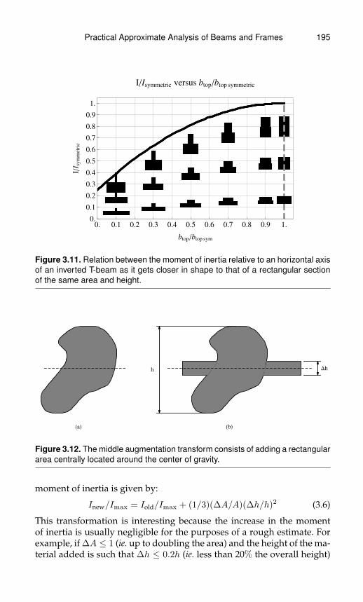
Practical Approximate Analysis of Beams and Frames 195
0. 0.1 0.2 0.3 0.4 0.5 0.6 0.7 0.8 0.9 1.0.
0.1
0.2
0.3
0.4
0.5
0.6
0.7
0.8
0.9
1.
btop�btop sym
I�Isym
metr
ic
I�Isymmetric versus btop�btop symmetric
Figure 3.11. Relation between the moment of inertia relative to an horizontal axisof an inverted T-beam as it gets closer in shape to that of a rectangular sectionof the same area and height.
Dhh
HaL HbL
Figure 3.12. The middle augmentation transform consists of adding a rectangulararea centrally located around the center of gravity.
moment of inertia is given by:
Inew/Imax = Iold/Imax + (1/3)(∆A/A)(∆h/h)2 (3.6)
This transformation is interesting because the increase in the momentof inertia is usually negligible for the purposes of a rough estimate. Forexample, if ∆A ≤ 1 (ie. up to doubling the area) and the height of the ma-terial added is such that ∆h ≤ 0.2h (ie. less than 20% the overall height)
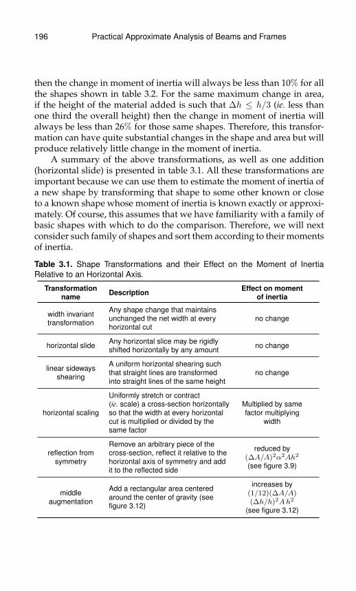
196 Practical Approximate Analysis of Beams and Frames
then the change in moment of inertia will always be less than 10% for allthe shapes shown in table 3.2. For the same maximum change in area,if the height of the material added is such that ∆h ≤ h/3 (ie. less thanone third the overall height) then the change in moment of inertia willalways be less than 26% for those same shapes. Therefore, this transfor-mation can have quite substantial changes in the shape and area but willproduce relatively little change in the moment of inertia.
A summary of the above transformations, as well as one addition(horizontal slide) is presented in table 3.1. All these transformations areimportant because we can use them to estimate the moment of inertia ofa new shape by transforming that shape to some other known or closeto a known shape whose moment of inertia is known exactly or approxi-mately. Of course, this assumes that we have familiarity with a family ofbasic shapes with which to do the comparison. Therefore, we will nextconsider such family of shapes and sort them according to their momentsof inertia.
Table 3.1. Shape Transformations and their Effect on the Moment of InertiaRelative to an Horizontal Axis.
Transformationname Description Effect on moment
of inertia
width invarianttransformation
Any shape change that maintainsunchanged the net width at everyhorizontal cut
no change
horizontal slide Any horizontal slice may be rigidlyshifted horizontally by any amount no change
linear sidewaysshearing
A uniform horizontal shearing suchthat straight lines are transformedinto straight lines of the same height
no change
horizontal scaling
Uniformly stretch or contract(ie. scale) a cross-section horizontallyso that the width at every horizontalcut is multiplied or divided by thesame factor
Multiplied by samefactor multiplying
width
reflection fromsymmetry
Remove an arbitrary piece of thecross-section, reflect it relative to thehorizontal axis of symmetry and addit to the reflected side
reduced by(∆A/A)2α2Ah2
(see figure 3.9)
middleaugmentation
Add a rectangular area centeredaround the center of gravity (seefigure 3.12)
increases by(1/12)(∆A/A)(∆h/h)2Ah2
(see figure 3.12)

Practical Approximate Analysis of Beams and Frames 197
Table 3.2. Relation Between Shape, Radius of Gyration and Height of Cross-Sections for Symmetric Sections. The Cross-Sectional Shapes are Rankedin(Usually) Decreasing Order of I /Imax where ‘I ’ is the Moment of Inertia of theCross-Section Relative to an Horizontal Axis and Imax = Ah2/4 is the MaximumPossible Moment of Inertia Relative to an Horizontal Axis for a Fixed Area ‘A’ andHeight ‘h.’
Note: In the table below, ‘A’ is the area, ‘b’ is the width, ‘h’ is the height, ‘ρ’ is theradius of gyration around an horizontal axis through the center of gravity, ‘I ’ is themoment of inertia around an horizontal axis through the center of gravity, ‘Imax’is the maximum possible moment of inertia, ‘r’ is the radius of a circle (if present)and ‘t’ is a thickness (if present).
Name Shape Area(A) ρ/h I/Imax
ideal I-beam 2bt 12
= 0.5 1
I-beam(Aweb � Aflange
) Aflange +Aweb
≈ 12
(1− 1
2AwebAflange
)≈(
1− AwebAflange
)hollow square ≈ 4ht ≈ 1
2√
1.5
(1− t
h
)≈(1− 2 t
h
)sharp-edged
parabolic hourglass13bh ≈ 1
2√
1.842= 0.368 ≈ 0.543
sharp-edged linearhourglass
12bh
12√
2≈ 0.354 1
2
hollow circular disk ≈ πrt ≈ 12√2
(1− t
4r
)≈ 1
2(1− t
2r
)rectangle bh
12√
3≈ 0.289 1
3
elliptic disk(includes circular)
π4bh
12×√
4= 0.250 1
4
facing parabolas 23bh
12√
4.375≈ 0.239 1
4.375
diamond 12bh
12√
6≈ 0.204 1
6
parabolas-sideddiamond
13bh
12√
7≈ 0.189 1
7
In order to compare and sort the moments of inertia we normalizethe moment of inertia relative to an horizontal axis by the maximumpossible moment of inertia which is Imax = Ah2/4. This gives a ratiowhich is always between zero and one. Also, since the displacement isinversely proportional to the moment of inertia, this ratio gives the rel-
198 Practical Approximate Analysis of Beams and Frames
ative rigidity of a given cross-section for a fixed area and height. Thehigher the ratio, the higher the rigidity of the cross-section with a ratioof one corresponding to the shapes with the highest possible rigidity fora given area and height. In addition, for symmetric cross-sections, themaximum stress is also inversely proportional to the moment of inertiafor a fixed area, height and maximum bending moment. Therefore, theratio I /Imax also gives the relative strength of a symmetric cross-sectionfor a fixed area and height. For example, a diamond shape and a rectan-gular shape (see table 3.2) have I /Imax equal to 1/6 and 1/3 respectively.Therefore, a beam with a rectangular cross-section is (1/3)/(1/6) = 2times as strong and as rigid as a diamond shaped cross-section for thesame area and height.
We start by discussing a set of cross-sectional shapes that are sym-metric relative to a horizontal axis and these are shown in table 3.2 (sec-ond column). From the definition of the moment of inertia, we expectthe moment of inertia for a given area to increase as more of the areais placed as far as possible from the center of gravity. In the limit, weget the ’ideal I-beam’ which has the area placed symmetrically at halfthe height away from the center of gravity. This configuration gives thehighest possible moment of inertia so that I /Imax = 1. The next con-figuration allows for a web or some material to be placed to connect thetwo areas placed at the farthest point. This gives an I-beam that can actu-ally be constructed and has a relatively lower moment of inertia than theideal I-beam. A shape that may be equivalent to a real I-beam in terms ofmoment of inertia is the hollow square (see figure 3.6) and is shown asthe third entry in table 3.2. The next two shapes considered allow forthe width to taper as we get closer to the center of gravity. They areboth hour-glass shaped but one has parabolic borders and the one afterthat has straight line borders. Both these hour-glass shaped cross-sectionwould need some small amount of material to be placed at and near thecenter of gravity in order to have a well-connected section but these donot much affect the moment of inertia. In any case, the parabolic and lin-ear hour-glass I /Imax equal about 0.543 and 0.5 respectively. The nextshape is that of the hollow circular disk which, depending on its thick-ness ‘t,’ may or may not be more efficient than the rectangular sectionwhich has I /Imax = 1/3. The rectangular cross-section is a delimitingcase between the shapes that taper out as we get farther from the centerof gravity and those that taper in. Of course, shapes that taper out willhave relatively higher moment of inertia for the same area and height.Among the rest of the shapes, we note the elliptic cross-sections whichinclude the disk and all of these sections have I /Imax = 1/4. We alsonote the diamond shape with straight edges which has I /Imax = 1/6.

Practical Approximate Analysis of Beams and Frames 199
Note that, with all the cross sections, if we have a specified heightand area, then this determines the width ‘b’ or thickness ‘t’ for a chosenshape. In particular, for the elliptic cross-sections, if we specify the heightand area, the width is then determined and this will generally not corre-spond to a disk or circular border. In any case, the formula for the area isalso given in order to obtain cross-sections that are comparable in termsof the moment of inertia when we specify both the area and the height.Finally, the radius of gyration relative to an horizontal axis is also givensince this could be useful in some applications.
Table 3.3. Relation Between Shape, Radius of Gyration and Height of Cross-Sections for Non-Symmetric Sections with Monotonically Varying Width. TheCross-Sectional Shapes are Ranked in (Mostly) Decreasing Order of I /Imax
where ‘I ’ is the Moment of Inertia of the Cross-Section and Imax = Ah2/4 is theMaximum Possible Moment of Inertia for the Same Area ‘A’ and Height ‘h’ of theCross Section. The Result for a Rectangle is also Given as a Limiting Case of theTrapezoid.
Note: In the table below, ‘A’ is the area, ‘b’ is the width, ‘h’ is the height, ‘ρ’ is theradius of gyration around an horizontal axis through the center of gravity, ‘I ’ is themoment of inertia around an horizontal axis through the center of gravity, ‘Imax’is the maximum possible moment of inertia, ‘r’ is the radius of a circle (if present)and ‘t’ is a thickness (if present).
Name Shape Area(A) ρ/h I/Imax
rectangle bh√
112
13
Trapezoid (bb+bt)2
h
√b2b+4bbbt+b
2t√
9/8(bb+bt)
29
(b2b+4bbbt+b2t )
(bb+bt)2
semi-elliptic π4bh
√9π2−646π
≈√1
14.31
1− 649π2 ≈ 1
3.58
outer-parabola 23bh
√1
14.591
3.65
triangle 12bh
√118
14.5
inner-parabola 13bh ≈
√1
18.92≈ 1
4.73
⊥− beam (flangethickness << h) Aw +Af ≈
√112
√AwA
≈ 13AwA
⊥− beamnegligible web A ≈ 0 ≈ 0

200 Practical Approximate Analysis of Beams and Frames
Finally, we discuss a set of cross-sectional shapes that are unsymmet-ric relative to an horizontal axis and these are shown in table 3.3 (secondcolumn). These shapes all have the property that the width is monoton-ically decreasing (or more precisely non-increasing) with the height. Ofcourse, these are a small subset of all possible shapes but the reflectionfrom symmetry and the middle augmentation allows us to estimate amuch wider set of non-symmetric shapes. As a delimiting case, we firstconsider the rectangular cross-section which remains constant throughthe height direction. This case which has I /Imax = 1/3 is an upperbound on all the other shapes in this set. For example, if we maximizethe value of I /Imax for the trapezoidal shape over all possible values ofbb (bottom width) and bt (upper width), we find that the maximum of1/3 occurs only when those widths are equal which gives a rectangularcross-section. Some interesting results in table 3.3 include:
• The semi-elliptic cross-section is about 10.55% more efficient than theelliptic cross-section. Note that this does not violate the reflection fromsymmetry because such a transformation cannot change an ellipticinto a semi-elliptic cross-section.
• The triangular cross-section is about 55.6% less efficient than thestraight-edged hour-glass but only 33.3% more effficient than thestraight-edged diamond both of which can be constructed from tri-angles.
3.3 Relative Vertical Displacementsversus Strain in Beams
The formulas and results presented so far require a knowledge of boththe load magnitude and the moment of inertia in order to determine thedisplacements. In some cases, such as during a visual inspection of abuilt structure or in preliminary design, it may be sufficient to approx-imately determine the range of displacements of a member. For such acase, an approach that only uses geometrical variables (ie. dimensionsand strain) will be desirable and related formulas and discussions forthis purpose will be developed in this section.
To illustrate the basic idea, we start with a simply supported beamsubject to a uniformly distributed load (figure 3.1b with kL = kR = 0).The maximum displacement for that case occurs at the middle and isgiven by:
δapplied max =5
384
qL4
EI(simply-supported beam) (3.7)
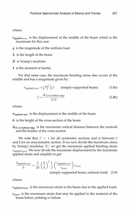
Practical Approximate Analysis of Beams and Frames 201
where:
δapplied max is the displacement at the middle of the beam which is themaximum for this case
q is the magnitude of the unifrom load
L is the length of the beam
E is Young’s modulus
I is the moment of inertia
For that same case, the maximum bending stress also occurs at themiddle and has a magnitude given by:
σapplied max = 18qL2
Ih2β (simply-supported beam) (3.8a)
β =dCG to farthest edge
h/2(3.8b)
where:
σapplied max is the displacement at the middle of the beam
h is the height of the cross-section of the beam
dCG to farthest edge is the maximum vertical distance between the centroidand the border of the cross-section
We note that β = 1 for all symmetric sections and is between 1and 2 for an unsymmetric section. If we now divide the maximum stressby Young’s modulue ‘E,’ we get the maximum applied bending strainεapplied max. We now divide the maximum displacement by the maximumapplied strain and simplify to get:
δapplied max
h=
5
24
(L
h
)21
β
(εapplied max
εmax
)εmax
(simply-supported beam; uniform load) (3.9)
where:
εapplied max is the maximum strain in the beam due to the applied loads
εmax is the maximum strain that may be applied to the material of thebeam before yielding or failure
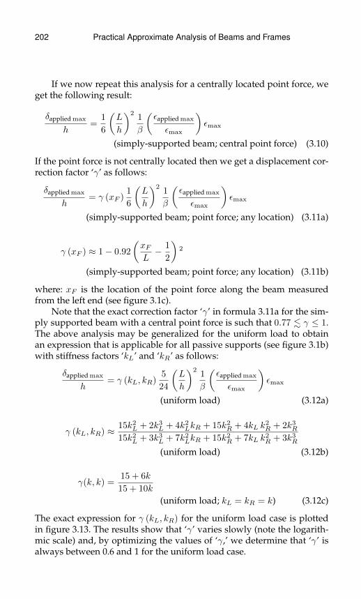
202 Practical Approximate Analysis of Beams and Frames
If we now repeat this analysis for a centrally located point force, weget the following result:
δapplied max
h=
1
6
(L
h
)21
β
(εapplied max
εmax
)εmax
(simply-supported beam; central point force) (3.10)
If the point force is not centrally located then we get a displacement cor-rection factor ‘γ’ as follows:
δapplied max
h= γ (xF )
1
6
(L
h
)21
β
(εapplied max
εmax
)εmax
(simply-supported beam; point force; any location) (3.11a)
γ (xF ) ≈ 1− 0.92
(xFL− 1
2
)2
(simply-supported beam; point force; any location) (3.11b)
where: xF is the location of the point force along the beam measuredfrom the left end (see figure 3.1c).
Note that the exact correction factor ‘γ’ in formula 3.11a for the sim-ply supported beam with a central point force is such that 0.77 . γ ≤ 1.The above analysis may be generalized for the uniform load to obtainan expression that is applicable for all passive supports (see figure 3.1b)with stiffness factors ‘kL’ and ‘kR’ as follows:
δapplied max
h= γ (kL, kR)
5
24
(L
h
)21
β
(εapplied max
εmax
)εmax
(uniform load) (3.12a)
γ (kL, kR) ≈ 15k2L + 2k3
L + 4k2LkR + 15k2
R + 4kL k2R + 2k3
R
15k2L + 3k3
L + 7k2LkR + 15k2
R + 7kL k2R + 3k3
R
(uniform load) (3.12b)
γ(k, k) =15 + 6k
15 + 10k
(uniform load; kL = kR = k) (3.12c)
The exact expression for γ (kL, kR) for the uniform load case is plottedin figure 3.13. The results show that ‘γ’ varies slowly (note the logarith-mic scale) and, by optimizing the values of ‘γ,’ we determine that ‘γ’ isalways between 0.6 and 1 for the uniform load case.
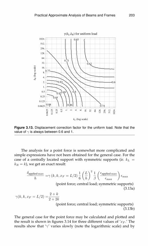
Practical Approximate Analysis of Beams and Frames 203
0.62
0.65
0.68
0.71
0.74
0.77
0.8
0.83
0.86
0.890.92
0.95
0.98
0.0
625
0.1
25
0.2
5
0.5 1.
2.
4.
8.
16.
32.
64.
128.
256.
512.
1024.
0.0625
0.125
0.25
0.5
1.
2.
4.
8.
16.
32.
64.
128.
256.
512.
1024.
kL Hlog scaleL
kRHl
og
scaleL
ΓHkL,kRL for uniform load
Figure 3.13. Displacement correction factor for the uniform load. Note that thevalue of γ is always between 0.6 and 1.
The analysis for a point force is somewhat more complicated andsimple expressions have not been obtained for the general case. For thecase of a centrally located support with symmetric supports (ie. kL =kR = k), we get an exact result:
δapplied max
h=γ (k, k, xF = L/2)
1
6
(L
h
)21
β
(εapplied max
εmax
)εmax
(point force; central load; symmetric supports)(3.13a)
γ(k, k, xF = L/2) =2 + k
2 + 2k
(point force; central load; symmetric supports)(3.13b)
The general case for the point force may be calculated and plotted andthe result is shown in figures 3.14 for three different values of ‘xF .’ Theresults show that ‘γ’ varies slowly (note the logarithmic scale) and by
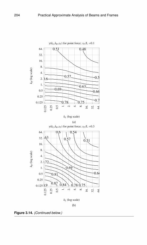
204 Practical Approximate Analysis of Beams and Frames
0.480.51
0.540.570.6
0.63
0.660.69
0.720.750.78
0.1
25
0.2
5
0.5 1
.
2.
4.
8.
16.
32.
64.
0.125
0.25
0.5
1.
2.
4.
8.
16.
32.
64.
kL Hlog scaleL
kRHl
og
scaleL
ΓHkL,kR,xFL for point force; xF�L =0.1
(a)
0.51
0.54
0.57
0.6
0.63
0.66
0.69
0.72
0.750.78
0.81
0.840.87
0.9
0.1
25
0.2
5
0.5 1
.
2.
4.
8.
16.
32.
64.
0.125
0.25
0.5
1.
2.
4.
8.
16.
32.
64.
kL Hlog scaleL
kRHl
og
scaleL
ΓHkL,kR,xFL for point force; xF�L =0.3
(b)
Figure 3.14. (Continued below.)
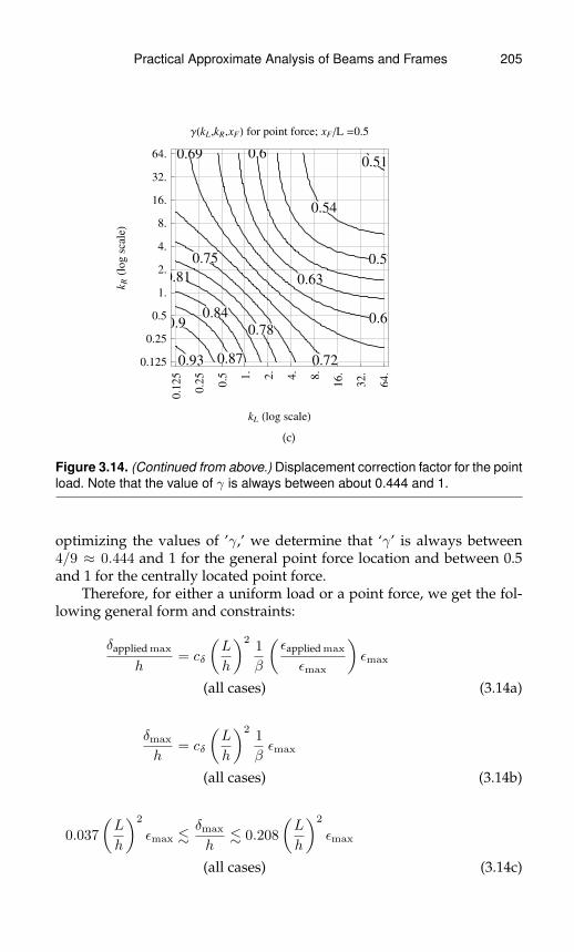
Practical Approximate Analysis of Beams and Frames 205
0.51
0.54
0.57
0.6
0.63
0.66
0.69
0.72
0.75
0.78
0.81
0.84
0.87
0.9
0.93
0.1
25
0.2
5
0.5 1
.
2.
4.
8.
16.
32.
64.
0.125
0.25
0.5
1.
2.
4.
8.
16.
32.
64.
kL Hlog scaleL
kRHl
og
scaleL
ΓHkL,kR,xFL for point force; xF�L =0.5
(c)
Figure 3.14. (Continued from above.) Displacement correction factor for the pointload. Note that the value of γ is always between about 0.444 and 1.
optimizing the values of ’γ,’ we determine that ‘γ’ is always between4/9 ≈ 0.444 and 1 for the general point force location and between 0.5and 1 for the centrally located point force.
Therefore, for either a uniform load or a point force, we get the fol-lowing general form and constraints:
δapplied max
h= cδ
(L
h
)21
β
(εapplied max
εmax
)εmax
(all cases) (3.14a)
δmax
h= cδ
(L
h
)21
βεmax
(all cases) (3.14b)
0.037
(L
h
)2
εmax .δmax
h. 0.208
(L
h
)2
εmax
(all cases) (3.14c)

206 Practical Approximate Analysis of Beams and Frames
2
27≤ cδ ≤
5
24(ie. 0.0741 . cδ . 0.208) (3.14d)
β =
{1 symmetric cross section1 < β < 2 non-symmetric cross-section
(3.14e)
εapplied max
εmax≤ 1 (3.14f)
where: δmax is the maximum possible displacement before the maximumallowable strain ‘εmax’ is reached somewhere in the beam.
The formula 3.14a is interesting for several reasons including:
• The maximum displacement (δmax) is independent of Young’s mod-ulus, the area of the cross-section, the width of the cross-section and,for a symmetric cross-section, the moment of inertia. In particular, wecan avoid calculating the maximum load as an intermediate step indetermining the maximum displacement.
• The maximum over minimum value of cδ is about 2.8 so that all beamswith a uniform or a point force load and with any type of passive con-nections will be within a relatively narrow range when the other vari-ables in formula 3.14a are specified.
• An upper bound on the maximum displacement (δmax) depends onlyon the ratio of length over height, height and material property ‘εmax.’This means that if we can estimate the material property ‘εmax’ ofthe beam and, by a simple visual inspection, estimate the length andheight of the beam, then we can estimate an upper bound on the max-imum displacement.
Using the relations in 3.14 we can get upper bounds on the maxi-mum displacement for different materials that may be encountered instructural engineering. Typical values of ‘εmax’ for some of those mate-rials are given in table 3.4. The table indicates that most materials havea maximum strain in the range of 0.1% to 1%. This means that the max-imum displacement for those materials must have an upper bound be-tween 0.000037(L/h)2h and 0.0021(L/h)2h. If the length to height ratiois between 5 to 20 then this means that the maximum possible displace-ment must have an upper bound between 0.0009h and 0.85h. This is awide range but it covers a very wide range of materials, loading condi-tions, length to height ratios and support conditions. For more precise
Practical Approximate Analysis of Beams and Frames 207
Table 3.4. Range of Maximum Strain in Common Structural Materials.
Material Typical rangeof εmax
note
Steel 0.1% to 0.3%Based on yield strengths oftypical structural steels
Aluminum 0.1% to 0.7%Based on yield strength of widerange of Aluminum types
Concrete 0.3% to 0.5%Based on ultimate strengths oflow to high strength concrete
Wood 0.02% to 0.08%Based on the compressionproportionality limit of soft andhard woods
Thermoplastics may be severalpercent
Varies widely, may be severalpercent
estimates, we may use a more specific formula from the ones presentedabove.
For example, consider a steel beam with symmetric cross-sectionwith εmax = 0.001 subject to a centrally applied point force which ishalf the maximum possible. In addition, the beam has a span of 5m andheight of 0.5m and it is connected to either side by identical beams. Inthis case, the maximum deflection may be estimated as follows: We startby using formula 3.13a with the stiffness factor k ≈ 1 and the ratio ofapplied maximum to maximum possible strain
(εapplied max/εmax
)= 0.5.
Using formula 3.13b or figure 3.14c, we get that γ = 3/4 and this thenleads to an estimate of the maximum deflection to be (3/4) × (1/6) ×(5m/0.5m)× 1× (0.5)× 0.001× 0.5m ≈ 0.0003125m = 0.3125mm. Notethat this is the maximum displacement due to half the failure load. Forthe full failure load due to a point force, we get double the previous dis-placement which is equivalent to 0.00125h (ie. within the bounds identi-fied previously).
For completion, we also present the formula equivalent to 3.14 for acantilever that is either uniformly loaded or loaded by a point force at itstip. The results are as follows:
δmax
h=
1
2
(L
h
)21
β
(εapplied max
εmax
)εmax
(uniform loaded cantilever) (3.15a)
δmax
h=
2
3
(L
h
)21
β
(εapplied max
εmax
)εmax
(point force at tip of a cantilever) (3.15b)

208 Practical Approximate Analysis of Beams and Frames
Note that the result of the point force may be inferred from the centralpoint force on a simply supported beam by doubling the effective lengthof the beam. The uniform load case cannot be similarly inferred becausedoubling the length with symmetry does not give a simply-supportedbeam with a uniform load. We note that the cantilever has a significantlyhigher maximum displacement at any given strain level and, in particu-lar, at failure than beams supported at both sides.
3.4 Side Displacements of FramesSubject to Side Loads
In this section, we will describe how to estimate the sidesway in a regularframe that would usually be part of a building. So far in our analysis, wehave assumed that axial deformations in the analysis of a frame may beneglected since they are much smaller than the bending deformations.While this will turn out to be true for most practical frames with fewerthan about 10 to 20 floors, we will investigate quantitatively the condi-tions under which if we neglect axial deformations then we still obtaingood approximation for the sideway movement of a frame.
To explore the conditions where we can neglect axial deformations,we consider a class of frames where all the beams have the same sectionalproperties and all the columns have the same sectional properties suchas the frame shown in figure 3.15. In addition, all the columns have thesame height and all the beams have the same length with a single sideforce applied at the top floor. We then consider the side deflection at thepoint where the load is applied and compare that value to the one wewould obtain if we neglect the axial deformations or equivalently whenEAc →∞ in figure 3.15. Based on this, we define the shear deformationfraction as the side deflection at the top floor when we neglect the axialdeformations divided by the same deflection when we do not neglectthose axial deformations. The shear deformation fraction must alwaysbe between zero and one When this fraction is close to one then we mayneglect axial deformations and conversely, when this fraction is close tozero then we may neglect shear deformations.
As a first step in our discussion, we derive an approximate expres-sion for both the shear and bending deformations for the class of build-ings depicted in figure 3.15. These expressions will be useful in clarifyingthe mechanisms and non-dimensional parameters that affect the sheardeformation fraction and in providing a more convenient expression todo parametric studies.
We start by considering the top floor displacements due to sheardeformations. This top floor displacement is the sum of the sidesways

Practical Approximate Analysis of Beams and Frames 209
Lb Lb Lb Lb
Lc
Lc
Lc
Lc
Lc
EIb
EIb
EIb
EIb
EIb
EIb
EIb
EIb
EIb
EIb
EIb
EIb
EIb
EIb
EIb
EIb
EIb
EIb
EIb
EIb
EIc
EAc
EIc
EAc
EIc
EAc
EIc
EAc
EIc
EAc
EIc
EAc
EIc
EAc
EIc
EAc
EIc
EAc
EIc
EAc
EIc
EAc
EIc
EAc
EIc
EAc
EIc
EAc
EIc
EAc
EIc
EAc
EIc
EAc
EIc
EAc
EIc
EAc
EIc
EAc
EIc
EAc
EIc
EAc
EIc
EAc
EIc
EAc
EIc
EAc
P
Figure 3.15. Class of building analyzed to identify contribution of bending versusaxial deformations due to horizontal loads.
(ie. difference in sideway movement of columns) of all the floors. In ad-dition, using free body diagrams at each floor and considering horizontalequilibrium, we find that the total of the shear forces in all the columns inany given floor equals the same force ‘P ’ that is applied at the top floor.Using the previously defined shear stiffness of a column, the sideswayof a given floor is then given by ‘P ’ divided by the total of the columnshear stiffnesses in that floor (eg. refer to the derivation of formula 2.9).Therefore, the horizontal displacement of one floor is given by:
sidesway of one floor ≈ P
stiffness of one floor
≈ 1
5 to 12
PL3c
EIc× 1
spans + 1≈(
11 + 6k
1 + 72k
)PL3
c
EIc× 1
spans + 1(3.16)

210 Practical Approximate Analysis of Beams and Frames
where:
P is the applied horizontal force at the top floor
Lc is the height of the columns
E is Young’s modulus
Ic is a column’s moment of inertia (assumed all uniform)
k is the ratio of a beam’s rotary stiffness divided by a column’s rotarystiffness (ie. k = (EIb/Lb) / (EIc/Lc))
spans is the number of spans (or bays) and spans + 1 equals the numberof columns in each floor
Note that to estimate the stiffness of a column in a building, wehave used formula 2.15 in spite of its limited applicability. By using for-mula 3.16 and summing over all floors, we get that the top floor displace-ment is given by:
δsheartop ≈(
11 + 6k
1 + 72k
)PL3
c
EIc× floors
spans + 1
=
(11 + 6k
1 + 72k
)PL2
cLbEIc
×(H
W
)spans
spans + 1(3.17)
=
(11 + 6k
1 + 72k
)PL2
cLbEIc
×(H
W
)floors
floors + (H/W ) (Lb/Lc)
where:
δsheartop is the side deflection of the top floor due to shear deformations
floors is the number of floors in the frame
H is the total height of the frame or building
W is the total width of the frame or building
Using parametric studies with EAc being very large, we find thatformula 3.17 gives results that have usually less than a few percent errorin the range of values that are of interest in subsequent discussions. Wenote that in all these studies, we assume that the axial elongations of thebeams are negligible even when the axial deformations in the columnsare taken into account.

Practical Approximate Analysis of Beams and Frames 211
Having considered the shear deformations in the class of frames con-sidered, we now focus on estimating the bending deformations in suchframes. To that purpose, we start by modelling the frame as an effectivecantilever subject to bending deformations only (ie. the usual Bernoullibeam or column). The top deflection of such a cantilever is given by:
δbending top =1
3
PH3
EIeff
where:
δbending top is the side deflection of the top floor due to bending deforma-tions
Ieff is the effective moment of inertia of the frame at any given floor
Therefore, we need to determine the effective moment of inertia inorder to obtain the required expression. To that purpose, we start (na-ively) to assume that each column acts like an area at a point with thecentroid being at the midpoint of any given floor. By summing up thecontribution of each column, we get the following result:
Ieff ≈ 12AcW
2 (1 + spans)(2 + spans)
6 spans(3.18)
Combining the above two expressions, we get:
δbending top ≈2
3
PH
EAc
(H
W
)26 spans
(1 + spans)(2 + spans)
=2
3
PH
EAc
(H
W
)3
× (3.19)
× 6 (Lb/Lc) floors(floors + (Lb/Lc) (H/W )
)(floors + 2 (Lb/Lc) (H/W )
)Using parametric studies, we find that while the above formula oftengives the right trend but it can have relatively large errors in the rangeof values that are of interest in subsequent discussions. Therefore, weneed to do a more careful study in order to obtain a more accurate ex-pression. However, the conceptual development of the above formula issimple and thus provides an overall idea of how we think about bendingdeformations.
In order to get a more accurate expression for the bending deforma-tions, we will consider a more detailed and discrete view of how bending

212 Practical Approximate Analysis of Beams and Frames
Lc�rGc = 5
Lc�rGc = 10
Lc�rGc = 20
Lc�rGc = 40
Lc�rGc = 80
-1.0 -0.5 0.5 1.0
-1.0
-0.5
0.5
1.0
Normalized axial forces in ground floor columns
Lb�Lc = 1.5; HEIb�LbL�HEIc�LcL = 3
Floors = 20; Spans = 8
Figure 3.16. Axial force variation as the slenderness ratio varies from a (very)short column to a slender column.
deformations develop in a frame. We start by considering the axial forcesin columns when a frame is subject to side forces. To get insight intothis problem we plot the normalized axial forces in the columns of theground floor of a frame with 20 floors and 8 spans and keeping otherparameters fixed, we vary the slenderness ratio of the columns as shownin figure 3.16. For realistic values of the slenderness ratio, we find thatthe distribution of axial deformations is far from linear. If we want to ap-proximate the axial forces, a suitable assumption is to consider that theonly non-zero axial forces are in the two outer columns.
The observation that only the outer columns have appreciable axialforces could be understood using the previously developed methods foranalyzing frames with sidesway. In particular, we note that for the typeof frame considered, and indeed for most frames that do not have inter-nal hinges, the inner columns all carry approximately the same amountof shear and, also, the shear in the outer columns are not much smaller.This leads to end moments in the columns of the same floor being ap-
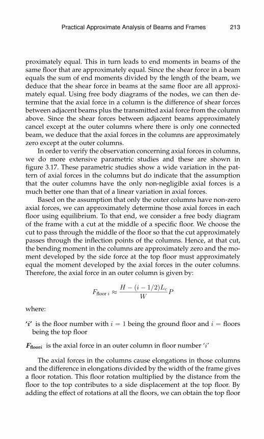
Practical Approximate Analysis of Beams and Frames 213
proximately equal. This in turn leads to end moments in beams of thesame floor that are approximately equal. Since the shear force in a beamequals the sum of end moments divided by the length of the beam, wededuce that the shear force in beams at the same floor are all approxi-mately equal. Using free body diagrams of the nodes, we can then de-termine that the axial force in a column is the difference of shear forcesbetween adjacent beams plus the transmitted axial force from the columnabove. Since the shear forces between adjacent beams approximatelycancel except at the outer columns where there is only one connectedbeam, we deduce that the axial forces in the columns are approximatelyzero except at the outer columns.
In order to verify the observation concerning axial forces in columns,we do more extensive parametric studies and these are shown infigure 3.17. These parametric studies show a wide variation in the pat-tern of axial forces in the columns but do indicate that the assumptionthat the outer columns have the only non-negligible axial forces is amuch better one than that of a linear variation in axial forces.
Based on the assumption that only the outer columns have non-zeroaxial forces, we can approximately determine those axial forces in eachfloor using equilibrium. To that end, we consider a free body diagramof the frame with a cut at the middle of a specific floor. We choose thecut to pass through the middle of the floor so that the cut approximatelypasses through the inflection points of the columns. Hence, at that cut,the bending moment in the columns are approximately zero and the mo-ment developed by the side force at the top floor must approximatelyequal the moment developed by the axial forces in the outer columns.Therefore, the axial force in an outer column is given by:
Ffloor i ≈H − (i− 1/2)Lc
WP
where:
‘i’ is the floor number with i = 1 being the ground floor and i = floorsbeing the top floor
Ffloori is the axial force in an outer column in floor number ‘i’
The axial forces in the columns cause elongations in those columnsand the difference in elongations divided by the width of the frame givesa floor rotation. This floor rotation multiplied by the distance from thefloor to the top contributes to a side displacement at the top floor. Byadding the effect of rotations at all the floors, we can obtain the top floor

214 Practical Approximate Analysis of Beams and Frames
-1.0 -0.5 0.5 1.0
-1.0
-0.5
0.5
1.0
Normalized axial forces in ground floor columns
Lb�Lc = 1.; Lc�rGc Hslenderness ratioL = 20
HEIb�LbL�HEIc�LcL = 1; Max floors = 10; Max spans = 10
(a)
-1.0 -0.5 0.5 1.0
-1.0
-0.5
0.5
1.0
Normalized axial forces in ground floor columns
Lb�Lc = 1.; Lc�rGc Hslenderness ratioL = 20
HEIb�LbL�HEIc�LcL = 3; Max floors = 10; Max spans = 10
(b)
Figure 3.17. (Continued below.)
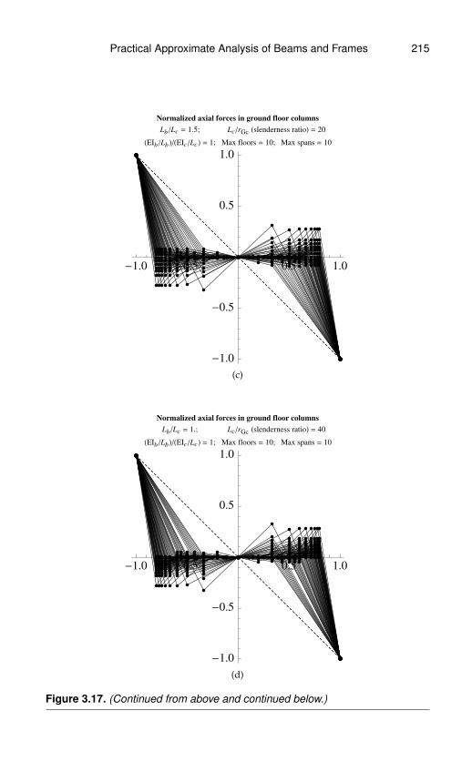
Practical Approximate Analysis of Beams and Frames 215
-1.0 -0.5 0.5 1.0
-1.0
-0.5
0.5
1.0
Normalized axial forces in ground floor columns
Lb�Lc = 1.5; Lc�rGc Hslenderness ratioL = 20
HEIb�LbL�HEIc�LcL = 1; Max floors = 10; Max spans = 10
(c)
-1.0 -0.5 0.5 1.0
-1.0
-0.5
0.5
1.0
Normalized axial forces in ground floor columns
Lb�Lc = 1.; Lc�rGc Hslenderness ratioL = 40
HEIb�LbL�HEIc�LcL = 1; Max floors = 10; Max spans = 10
(d)
Figure 3.17. (Continued from above and continued below.)
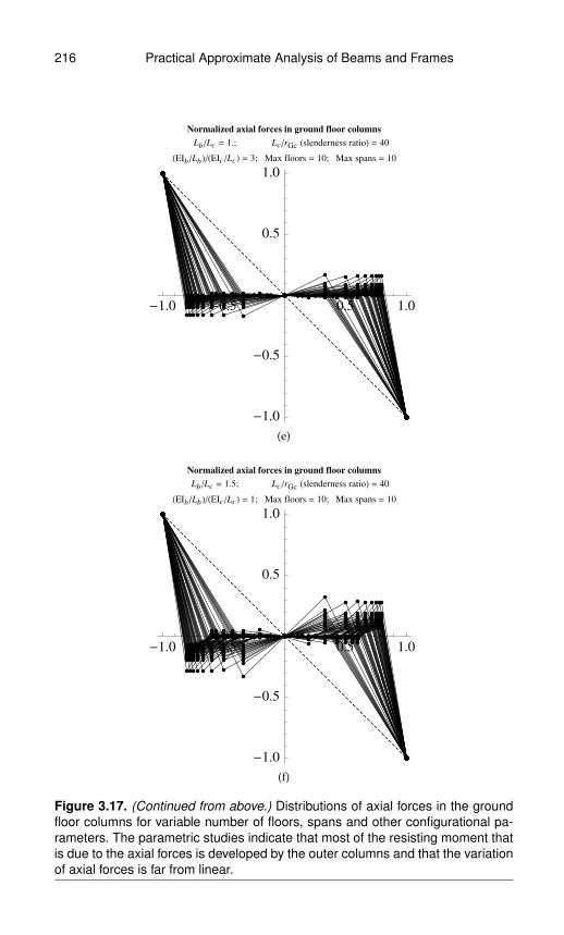
216 Practical Approximate Analysis of Beams and Frames
-1.0 -0.5 0.5 1.0
-1.0
-0.5
0.5
1.0
Normalized axial forces in ground floor columns
Lb�Lc = 1.; Lc�rGc Hslenderness ratioL = 40
HEIb�LbL�HEIc�LcL = 3; Max floors = 10; Max spans = 10
(e)
-1.0 -0.5 0.5 1.0
-1.0
-0.5
0.5
1.0
Normalized axial forces in ground floor columns
Lb�Lc = 1.5; Lc�rGc Hslenderness ratioL = 40
HEIb�LbL�HEIc�LcL = 1; Max floors = 10; Max spans = 10
(f)
Figure 3.17. (Continued from above.) Distributions of axial forces in the groundfloor columns for variable number of floors, spans and other configurational pa-rameters. The parametric studies indicate that most of the resisting moment thatis due to the axial forces is developed by the outer columns and that the variationof axial forces is far from linear.

Practical Approximate Analysis of Beams and Frames 217
displacement. The rotation ∆θfloori at the ith floor is given by:
∆θfloor i ≈ 2Ffloor iLcEAc
/W =
H − (i− 1/2)LcEAcW
2LcP
Multiplying this rotation by the distance from the floor to the top andadding the effect of all floors gives the top displacement:
δbending top ≈(1 + floors)(4 floors− 1)
6 floors2
PH
EAc
(H
W
)2
(3.20)
Using parametric studies, we find that formula 3.20 gives results witherrors that are usually less than about 15% and generally much lower inthe range of values that are of interest in subsequent discussions. Basedon formulas 3.17 and 3.20, we obtain the shear deformation fraction as:
shear fraction =δshear top
δtotal=
δshear top
δshear top + δbending top
⇒ shear fraction ≈ 1
1 +(floors +1)(4 floors−1)(spans +1)
6 floors2
(1+72k11+6k
)(Lc
rGc
)2(HW
)2⇒ shear fraction = z (3.21)
where:
z =1
1 + 23
(floors+1)(floors− 14 )(floors+(H/W )(Lb/Lc))
floors2
(1+72k11+6k
)(rGc
Lc
)2(HW
)(Lc
Lb
)and:
rGc is the radius of gyration of the column
(Lc/rGc) is the slenderness ratio
Parametric studies were done in order to determine the accuracy offormula 3.21 for the class of frames represented by figure 3.15. Specifi-cally, 500 cases were generated using the following rules:
• ‘k,’ the slenderness ratio and Lb/Lc were chosen randomly based onuniform distributions between 1 and 5, between 10 and 100 and be-tween 1 and 2 respectively.
• The number of floors was randomly chosen from the list (5, 10, 20, 40).
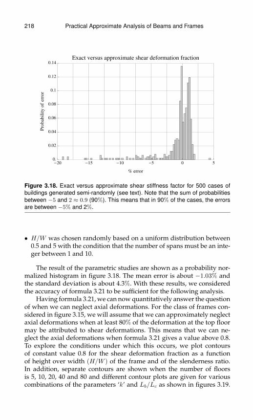
218 Practical Approximate Analysis of Beams and Frames
-20 -15 -10 -5 0 50.
0.02
0.04
0.06
0.08
0.1
0.12
0.14
% error
Pro
babil
ity
of
err
or
Exact versus approximate shear deformation fraction
Figure 3.18. Exact versus approximate shear stiffness factor for 500 cases ofbuildings generated semi-randomly (see text). Note that the sum of probabilitiesbetween −5 and 2 ≈ 0.9 (90%). This means that in 90% of the cases, the errorsare between −5% and 2%.
• H/W was chosen randomly based on a uniform distribution between0.5 and 5 with the condition that the number of spans must be an inte-ger between 1 and 10.
The result of the parametric studies are shown as a probability nor-malized histogram in figure 3.18. The mean error is about −1.03% andthe standard deviation is about 4.3%. With these results, we consideredthe accuracy of formula 3.21 to be sufficient for the following analysis.
Having formula 3.21, we can now quantitatively answer the questionof when we can neglect axial deformations. For the class of frames con-sidered in figure 3.15, we will assume that we can approximately neglectaxial deformations when at least 80% of the deformation at the top floormay be attributed to shear deformations. This means that we can ne-glect the axial deformations when formula 3.21 gives a value above 0.8.To explore the conditions under which this occurs, we plot contoursof constant value 0.8 for the shear deformation fraction as a functionof height over width (H/W ) of the frame and of the slenderness ratio.In addition, separate contours are shown when the number of floorsis 5, 10, 20, 40 and 80 and different contour plots are given for variouscombinations of the parameters ‘k’ and Lb/Lc as shown in figures 3.19.
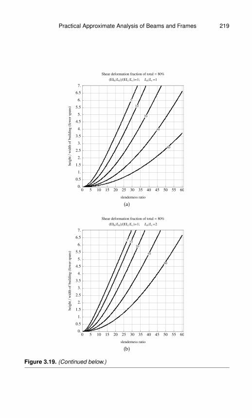
Practical Approximate Analysis of Beams and Frames 219
5
10
20
40
80
0 5 10 15 20 25 30 35 40 45 50 55 600.
0.5
1.
1.5
2.
2.5
3.
3.5
4.
4.5
5.
5.5
6.
6.5
7.
slenderness ratio
heig
ht�
wid
thof
buil
din
gHf
ew
er
spansL
Shear deformation fraction of total = 80%
HEIb�LbL�HEIc�LcL=1; Lb�Lc=1
(a)
510
20
40
80
0 5 10 15 20 25 30 35 40 45 50 55 600.
0.5
1.
1.5
2.
2.5
3.
3.5
4.
4.5
5.
5.5
6.
6.5
7.
slenderness ratio
heig
ht�
wid
thof
buil
din
gHf
ew
er
spansL
Shear deformation fraction of total = 80%
HEIb�LbL�HEIc�LcL=1; Lb�Lc=2
(b)
Figure 3.19. (Continued below.)

220 Practical Approximate Analysis of Beams and Frames
5
10
20
40
80
0 5 10 15 20 25 30 35 40 45 50 55 600.
0.5
1.
1.5
2.
2.5
3.
3.5
4.
4.5
5.
5.5
6.
6.5
7.
slenderness ratio
heig
ht�
wid
thof
buil
din
gHf
ew
er
spansL
Shear deformation fraction of total = 80%
HEIb�LbL�HEIc�LcL=3; Lb�Lc=1
(c)
5
10
20
40
80
0 5 10 15 20 25 30 35 40 45 50 55 600.
0.5
1.
1.5
2.
2.5
3.
3.5
4.
4.5
5.
5.5
6.
6.5
7.
slenderness ratio
heig
ht�
wid
thof
buil
din
gHf
ew
er
spansL
Shear deformation fraction of total = 80%
HEIb�LbL�HEIc�LcL=3; Lb�Lc=2
(d)
Figure 3.19. (Continued from above.) Fraction of top-left displacement attributedto shear in a building where only the top floor is loaded by a side-force. Curvesare labelled according to the number of floors (5, 10, 20, 40 and 80 floors) andtheir pattern indicate the fraction that may be attributed to shear deformation.The contours correspond to a shear deformation fraction of 80% of the totaldeformation.
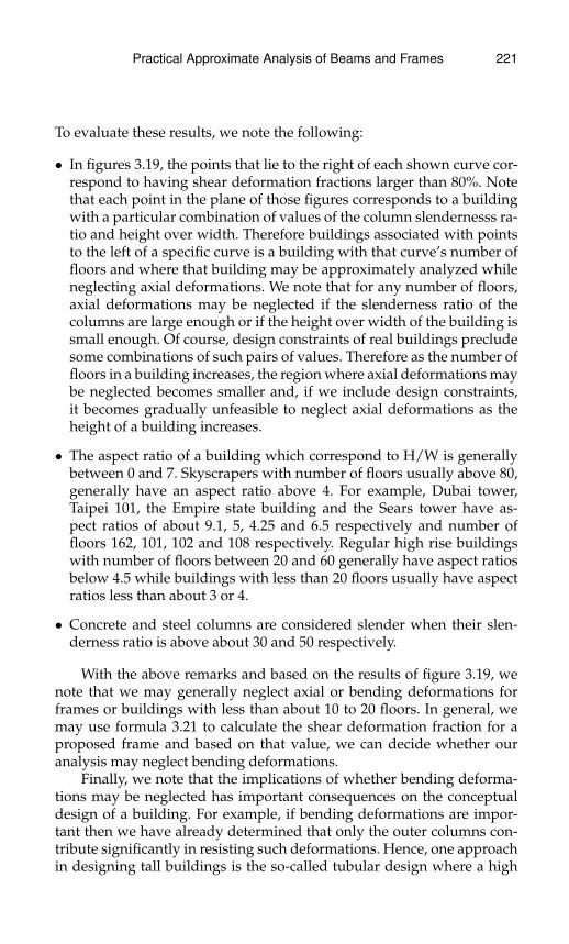
Practical Approximate Analysis of Beams and Frames 221
To evaluate these results, we note the following:
• In figures 3.19, the points that lie to the right of each shown curve cor-respond to having shear deformation fractions larger than 80%. Notethat each point in the plane of those figures corresponds to a buildingwith a particular combination of values of the column slendernesss ra-tio and height over width. Therefore buildings associated with pointsto the left of a specific curve is a building with that curve’s number offloors and where that building may be approximately analyzed whileneglecting axial deformations. We note that for any number of floors,axial deformations may be neglected if the slenderness ratio of thecolumns are large enough or if the height over width of the building issmall enough. Of course, design constraints of real buildings precludesome combinations of such pairs of values. Therefore as the number offloors in a building increases, the region where axial deformations maybe neglected becomes smaller and, if we include design constraints,it becomes gradually unfeasible to neglect axial deformations as theheight of a building increases.
• The aspect ratio of a building which correspond to H/W is generallybetween 0 and 7. Skyscrapers with number of floors usually above 80,generally have an aspect ratio above 4. For example, Dubai tower,Taipei 101, the Empire state building and the Sears tower have as-pect ratios of about 9.1, 5, 4.25 and 6.5 respectively and number offloors 162, 101, 102 and 108 respectively. Regular high rise buildingswith number of floors between 20 and 60 generally have aspect ratiosbelow 4.5 while buildings with less than 20 floors usually have aspectratios less than about 3 or 4.
• Concrete and steel columns are considered slender when their slen-derness ratio is above about 30 and 50 respectively.
With the above remarks and based on the results of figure 3.19, wenote that we may generally neglect axial or bending deformations forframes or buildings with less than about 10 to 20 floors. In general, wemay use formula 3.21 to calculate the shear deformation fraction for aproposed frame and based on that value, we can decide whether ouranalysis may neglect bending deformations.
Finally, we note that the implications of whether bending deforma-tions may be neglected has important consequences on the conceptualdesign of a building. For example, if bending deformations are impor-tant then we have already determined that only the outer columns con-tribute significantly in resisting such deformations. Hence, one approachin designing tall buildings is the so-called tubular design where a high
222 Practical Approximate Analysis of Beams and Frames
percent of the area of all columns are preferentially positioned on theoutside of the building. Other approaches that use local or global cross-bracings may also be used either to enhance the contribution of innercolumns or to provide an independent second system that is resistant tobending. However, the design of tall buildings is outside the scope of thisbook. Based on the above study, the methods presented in this book foranalyzing frames with sidesway are mostly suitable for buildings withless than about 10 to 20 floors.
3.5 Obtaining Rotary Stiffness Factorsfrom Slope Measurements in Beams
In this book, we have extensively relied on the notion of rotary stiffnessfactors in order to approximately analyze beams and frames. In this sec-tion, we will consider how we can indirectly identify the stiffness factorsat the ends of a member in a beam or frame by measuring slopes onthat member. A procedure of this kind is important in providing a non-destructive test to determine whether the assumptions used in designinga continuous beam or a frame structure are actually realized in the builtstructure. This procedure is also important in doing a structural integrityassessment of a structure that may have been damaged due to environ-mental factors such as earthquakes or due to man-made factors such asaccidents.
In designing a process to identify the stiffness factors, we must de-cide on what to measure, what and how much load to apply and howto process the data to obtain the rotary stiffness factors. We also need todetermine the accuracy of our results and especially their sensitivity tomeasurement errors. We will discuss each of these items next.
First, we consider the choice of what to measure. In general, we needto measure some aspect of deformation such as strain, displacements orrotations. Preparing a member for strain measurements is tedious andtime-consuming especially on a built structure. On the other hand, dis-placement measurements require some reliable fixed datum which maybe difficult to achieve. Finally, slope measurements seem to be both eco-nomical and relatively fast. Of course, in any such choice, we will be mea-suring changes in the chosen variable due to an applied load increment.For slope measurements, we place an inclinometer (ie. device for measur-ing slope), make a measurement before we apply a load increment andthis will be our datum. As a subsequent step, we load the member andthen get a new measurement. The change in slope due to the incrementin load that we have applied will be the measurement which we will useto determine the rotary stiffness factors.

Practical Approximate Analysis of Beams and Frames 223
Since we are proposing to measure slope, it is useful to first iden-tify the resolution with which the slope may be measured. This resolu-tion will determine whether such an approach is feasible, the magnitudeof the incremental load to apply and the limits in accuracy with whichwe can infer the stiffness factors. For example, if the maximum possi-ble load increment causes failure at slopes below the resolution of theavailable inclinometers then we cannot use slope measurements, at thecurrent technology, to indirectly measure rotary stiffness factors. As theresolution gets sufficiently fine, we then get a trade-off between apply-ing smaller load increments and having higher accuracy in the inferredstiffness factors. If the load increment is too small then we may again fallbelow the resolution of our measuring instrument. On the other hand,we must generally stay well below the load at which failure occurs. Itwould be useful in our analysis to specify a minimum load increment.For this purpose, we choose a minimum load increment which shouldbe both convenient and safe to be around 20% of the maximum possi-ble load. Of course, this value is somewhat arbitrary and for differentapplications, this minimum load increment may be varied subject to ananalysis of the implied errors.
In order to determine whether a particular resolution in the measure-ment of slope is sufficient, we compare it with the maximum possibleslope when subjected to the minimum load increment. For that purpose,we can determine the maximum applied rotation in a beam in terms ofthe maximum possible strain similar to what we have done in a previoussection with the maximum applied displacement. The result is given by:
θapplied max = cθ
(L
h
)1
β
(εapplied max
εmax
)εmax (3.22a)
14 ≤ cθ ≤
23 (ie. 0.25 . cδ . 0.667 ) (3.22b)
In addition, at the time of the writing of this book (late 2009), com-mercially available and relatively cheap inclinometers have resolutionsof less than about 1.74 × 10⁻⁵ radians (ie. less than 0.001◦). Now thatwe have a formula for the maximum proposed slope that we need tomeasure and a resolution limit for available measuring devices, we cancompare the two to determine whether the proposed method is feasible.For example, if we consider a beam with length over height of 8, with asymmetric section, with a maximum load increment of 20% and a max-imum possible strain of 0.001, then the maximum applied slope in thebeam must be less than (1/4) × (8) × (1) × (0.2) × 0.001 ≈ 0.0004. Thisvalue is then 0.0004/0.0000174 ≈ 23 times the resolution limit. There-fore, for this case, we expect slope increments over a considerable part

224 Practical Approximate Analysis of Beams and Frames
of the span to be above the measurement resolution limit. However, theresolution limit is about 4.35% of the maximum slope that we propose tomeasure. Whether this implies an adequately low potential error to al-low a determination of the stiffness factors within a sufficiently narrowrange is a subject of further study which will be partially addressed inthis section.
We now consider the setup and the process for doing the measure-ments and for inferring the stiffness factors. As before, we consider abeam with passive supports as shown in figure 3.20. We propose to mea-sure the change in slopes at four locations due to a point force applied atthe middle of the beam. Specifically, the locations are at either end andand at a quarter the length from each end as indicated in figure 3.20. Theprocedure consists of the following steps: i) we measure the slopes beforeany load is applied, ii) we apply a point force at the middle, iii) measurethe slopes again and iv) the change in slopes at each of the four locationsare the measurements we will use to infer the rotary stiffness factors.Note that it is possible, but much more cumbersome and error prone,to do the procedure with a single tiltmeter. This would require placingthe tiltmeter at each of the locations in turn, taking a reference or datummeasurement with no load applied anywhere on the beam, placing thepoint force at the middle of the beam and repeating the measurements ateach location with the load kept in place.
kR´4
EI
L
kL´4
EI
L
xF=L�2
L
P
0.25L 0.25Ltiltmeter tiltmeter tiltmeter tiltmeter
Figure 3.20. Setup for experimentally identifying the stiffness factors kL and kR.
The reason for choosing the specific locations shown in figure 3.20 isthat, in this case, we can obtain each of the two stiffness factors separatelyin terms of the measured changes in slope. We start by determining theslopes in terms of the central point force which are given as:
Practical Approximate Analysis of Beams and Frames 225
∆θ0 = − 3 + 2kR48 + 64kL + 64kR + 64kL kR
PL2
EI+ e0 (3.23a)
∆θ1/4 = − 18 + 13kL + 11kR + 8kL kR384 + 512kL + 512kR + 512kL kR
PL2
EI+ e1/4 (3.23b)
∆θ3/4 =18 + 11kL + 13kR + 8kL kR
384 + 512kL + 512kR + 512kL kR
PL2
EI+ e3/4 (3.23c)
∆θ1 =3 + 2kL
48 + 64kL + 64kR + 64kL kR
PL2
EI+ e1 (3.23d)
where:
∆θ0, ∆θ1/4, ∆θ3/4 and ∆θ1 are the four changes in slope from left toright in figure 3.20
kL and kR are the left and right rotary stiffness factors
P is the magnitude of the point force applied at the middle of the beam
L is the length of the beam
E is Young’s modulus
I is the moment of inertia
e0, e1/4, e3/4 and e1 are the errors in measurements
Assuming for now that the errors e0, e1/4, e3/4 and e1 are zero, wenow calculate the following combinations of the changes in slopes:
mL = |∆θ0|/(∣∣∆θ1/4
∣∣+∣∣∆θ3/4
∣∣) = 2/(3 + 2kL) (3.24a)
mR = |∆θ1|/(∣∣∆θ1/4
∣∣+∣∣∆θ3/4
∣∣) = 2/(3 + 2kR) (3.24b)
where: | · | denotes the absolute value of a quantityNote that since the stiffness factors must be positive, then the com-
binations mL and mR must be between 0 and 2/3. From formulas 3.24aand b, we can solve for the stiffness factors as follows:
kL =2− 3mL
2mL(3.25a)
kR =2− 3mR
2mR(3.25b)
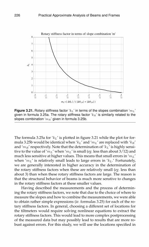
226 Practical Approximate Analysis of Beams and Frames
0
12
1
12
2
12
3
12
4
12
5
12
6
12
7
12
8
12
0
1
2
3
4
5
6
7
8
mL=È DΘ0 È � H ÈDΘ1�4È + ÈDΘ3�4È L
kL
Rotary stiffness factor in terms of slope combination 'm'
Figure 3.21. Rotary stiffness factor ‘kL’ in terms of the slopes combination ‘mL’given in formula 3.25a. The rotary stiffness factor ‘kR’ is similarly related to theslopes combination ‘mR’ given in formula 3.25b.
The formula 3.25a for ‘kL’ is plotted in figure 3.21 while the plot for for-mula 3.25b would be identical when ‘kL’ and ‘mL’ are replaced with ‘kR’and ‘mR’ respectively. Note that the determination of ‘kL’ is highly sensi-tive to the value of ‘mL’ when ‘mL’ is small (eg. less than about 3/12) andmuch less sensitive at higher values. This means that small errors in ‘mL’when ‘mL’ is relatively small leads to large errors in ‘kL.’ Fortunately,we are generally interested in higher accuracy in the determination ofthe rotary stiffness factors when these are relatively small (eg. less thanabout 3) than when these rotary stiffness factors are large. The reason isthat the structural behavior of beams is much more senstive to changesin the rotary stiffness factors at these smaller values.
Having described the measurements and the process of determin-ing the rotary stiffness factors, we note that due to the choice of where tomeasure the slopes and how to combine the measurements, we were ableto obtain rather simple expressions (ie. formulas 3.25) for each of the ro-tary stiffness factors. In general, choosing a different set of locations forthe tiltmeters would require solving nonlinear equations to extract therotary stiffness factors. This would lead to more complex postprocessingof the measured data but may possibly lead to results that are more ro-bust against errors. For this study, we will use the locations specified in
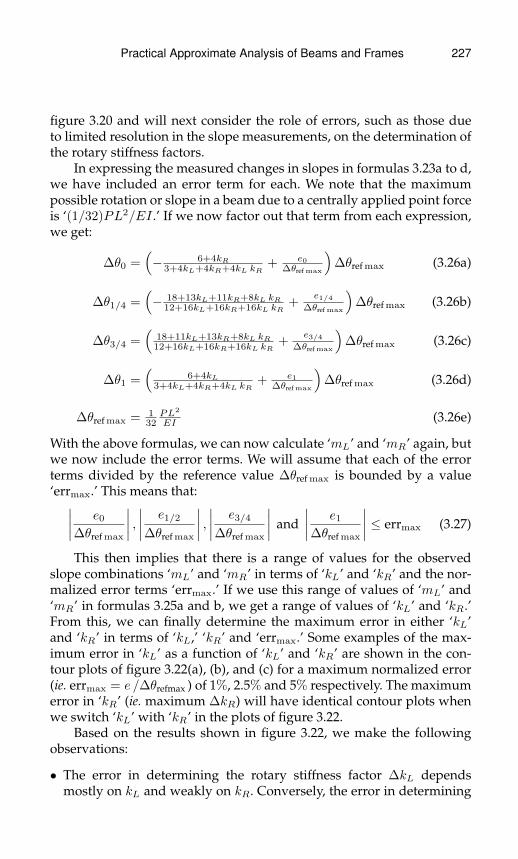
Practical Approximate Analysis of Beams and Frames 227
figure 3.20 and will next consider the role of errors, such as those dueto limited resolution in the slope measurements, on the determination ofthe rotary stiffness factors.
In expressing the measured changes in slopes in formulas 3.23a to d,we have included an error term for each. We note that the maximumpossible rotation or slope in a beam due to a centrally applied point forceis ‘(1/32)PL2/EI .’ If we now factor out that term from each expression,we get:
∆θ0 =(− 6+4kR
3+4kL+4kR+4kL kR+ e0
∆θref max
)∆θref max (3.26a)
∆θ1/4 =(− 18+13kL+11kR+8kL kR
12+16kL+16kR+16kL kR+
e1/4∆θref max
)∆θref max (3.26b)
∆θ3/4 =(
18+11kL+13kR+8kL kR12+16kL+16kR+16kL kR
+e3/4
∆θref max
)∆θref max (3.26c)
∆θ1 =(
6+4kL3+4kL+4kR+4kL kR
+ e1∆θref max
)∆θref max (3.26d)
∆θref max = 132PL2
EI (3.26e)
With the above formulas, we can now calculate ‘mL’ and ‘mR’ again, butwe now include the error terms. We will assume that each of the errorterms divided by the reference value ∆θref max is bounded by a value‘errmax.’ This means that:∣∣∣∣ e0
∆θref max
∣∣∣∣ , ∣∣∣∣ e1/2
∆θref max
∣∣∣∣ , ∣∣∣∣ e3/4
∆θref max
∣∣∣∣ and∣∣∣∣ e1
∆θref max
∣∣∣∣ ≤ errmax (3.27)
This then implies that there is a range of values for the observedslope combinations ‘mL’ and ‘mR’ in terms of ‘kL’ and ‘kR’ and the nor-malized error terms ‘errmax.’ If we use this range of values of ‘mL’ and‘mR’ in formulas 3.25a and b, we get a range of values of ‘kL’ and ‘kR.’From this, we can finally determine the maximum error in either ‘kL’and ‘kR’ in terms of ‘kL,’ ‘kR’ and ‘errmax.’ Some examples of the max-imum error in ‘kL’ as a function of ‘kL’ and ‘kR’ are shown in the con-tour plots of figure 3.22(a), (b), and (c) for a maximum normalized error(ie. errmax = e /∆θrefmax ) of 1%, 2.5% and 5% respectively. The maximumerror in ‘kR’ (ie. maximum ∆kR) will have identical contour plots whenwe switch ‘kL’ with ‘kR’ in the plots of figure 3.22.
Based on the results shown in figure 3.22, we make the followingobservations:
• The error in determining the rotary stiffness factor ∆kL dependsmostly on kL and weakly on kR. Conversely, the error in determining
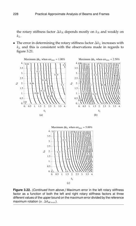
228 Practical Approximate Analysis of Beams and Frames
the rotary stiffness factor ∆kR depends mostly on kR and weakly onkL.
• The error in determining the rotary stiffness factor ∆kL increases withkL and this is consistent with the observations made in regards tofigure 3.21.
0.02
0.04
0.06
0.08
0.1
0.12
0.14
0.16
0.18
0.2
0.25
0.3
0.35
0. 0.5 1. 1.5 2. 2.5 3. 3.5 4.
0.
0.5
1.
1.5
2.
2.5
3.
3.5
4.
kL
kR
Maximum DkL when errmax = 1.00%
(a)
0.06
0.08
0.1
0.12
0.14
0.16
0.18
0.2
0.25
0.3
0.35
0.4
0.45
0.5
0.55
0.6
0.65
0.7
0.75
0.8
0.85
0.9
0. 0.5 1. 1.5 2. 2.5 3. 3.5 4.
0.
0.5
1.
1.5
2.
2.5
3.
3.5
4.
kL
kR
Maximum DkL when errmax = 2.50%
(b)
0.1
0.2
0.3
0.4
0.5
0.6
0.7
0.8
0.9
1
1.1
1.2
1.3
1.4
1.5
1.6
1.7
1.8
1.9
2
0. 0.5 1. 1.5 2. 2.5 3. 3.5 4.
0.
0.5
1.
1.5
2.
2.5
3.
3.5
4.
kL
kR
Maximum DkL when errmax = 5.00%
(c)
Figure 3.22. (Continued from above.) Maximum error in the left rotary stiffnessfactor as a function of both the left and right rotary stiffness factors at threedifferent values of the upper bound on the maximum error divided by the referencemaximum rotation (ie. ∆θref max).

Practical Approximate Analysis of Beams and Frames 229
• The values of ∆kL are neither expected errors nor confidence intervalwidth. They are bounds on the error in determining the rotary stiffnessfactor when the errors have a strict upper bound. Thus, while theseresults do not have a probabilistic interpretation, they are sufficientfor the purposes of giving an indication of the expected accuracy indetermining rotary stiffness factors due to a limitation in the resolutionof the measuring instruments.
Finally, based on the above study, we conclude that using currenttechnology, it is plausible to indirectly measure rotary stiffness factorsusing tiltmeters and reasonable loads applied on beams that are part of alarger structure. A process was outlined on how to do the measurements,how to postprocess them and how to estimate errors in the determina-tion of rotary stiffness factors due to possible measurement errors. Whatis not available at this time is an experimental study that verifies thesestatements. The usefulness of such a study in the structural integrity as-sessment of framed structures could be significant.

This page intentionally left blank
Chapter 4
Approximate InfluenceLines for IndeterminateBeams
4.1 Introduction to Influence LinesIn structural analysis, we are often interested in the effect of movingloads. For example, to design a bridge against failure, we would need toknow how the bending moment at its middle varies as a ‘standard’ car ortruck moves across its span. This requires consideration of the bendingmoment at a fixed point for every possible location of the car or truck.Using basic structural analysis, we would parametrize the location of thecar or truck on the bridge and then plot the bending moment at the centerversus this variable location. This plot would then constitute a succinctdescription of the influence of the car or truck on the bending moment atthe middle of the bridge. If, in this process, we replace the car or truck bya unit point force (ie. a single point force with magnitude one) then weget the influence line for the bending moment at the middle point of thebridge. Using that influence line, we can then use linear superposition toobtain the previously considered influence of a car or truck.
In general, we consider a frame or continuous beam as shown infigure 4.1 and a unit point force moving across that structure. As thatunit point force moves across the continuous beam ABCD, we monitoror calculate a response at any chosen but fixed point E. We call the fixedpoint E to be the point of influence or the influence point. If we plotthe response at point E as a function of the location of the unit pointforce along the continuous beam then we get the influence line of thatresponse as shown in figure 4.1. In general, the choice of response maybe the displacement, the rotation, the shear or the bending moment atthe chosen point. In addition, if the response is at a support, then theresponse may also be chosen as any of the reactions at that support.
231
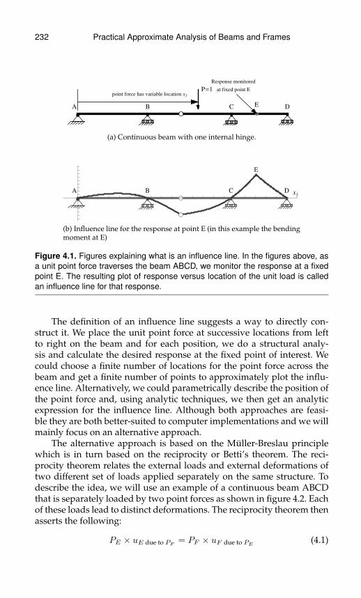
232 Practical Approximate Analysis of Beams and Frames
A B C D
P=1point force has variable location x f
E
Response monitored
at fixed point E
(a) Continuous beam with one internal hinge.
A B C D
E
0.15 0.3 0.45 0.6 0.75 0.9 1.05 1.2 1.35 1.5 1.65 1.8 1.95 2.1 2.25 2.4 2.55 2.7 2.85 3. 3.15
- 0.3
- 0.25
- 0.2
- 0.15
- 0.1
- 0.05
0.05
0.1
0.15
0.2
0.25
0.3
0.35
0.4
0.45
x f
(b) Influence line for the response at point E (in this example the bendingmoment at E)
Figure 4.1. Figures explaining what is an influence line. In the figures above, asa unit point force traverses the beam ABCD, we monitor the response at a fixedpoint E. The resulting plot of response versus location of the unit load is calledan influence line for that response.
The definition of an influence line suggests a way to directly con-struct it. We place the unit point force at successive locations from leftto right on the beam and for each position, we do a structural analy-sis and calculate the desired response at the fixed point of interest. Wecould choose a finite number of locations for the point force across thebeam and get a finite number of points to approximately plot the influ-ence line. Alternatively, we could parametrically describe the position ofthe point force and, using analytic techniques, we then get an analyticexpression for the influence line. Although both approaches are feasi-ble they are both better-suited to computer implementations and we willmainly focus on an alternative approach.
The alternative approach is based on the Muller-Breslau principlewhich is in turn based on the reciprocity or Betti’s theorem. The reci-procity theorem relates the external loads and external deformations oftwo different set of loads applied separately on the same structure. Todescribe the idea, we will use an example of a continuous beam ABCDthat is separately loaded by two point forces as shown in figure 4.2. Eachof these loads lead to distinct deformations. The reciprocity theorem thenasserts the following:
PE × uE due to PF= PF × uF due to PE
(4.1)

Practical Approximate Analysis of Beams and Frames 233
PEA B C D
E
F
uE due to PE
uF due to PE
Point force at E
PF
A B C D
E
F
uE due to PF
uF due to PF
Point force at F
Figure 4.2. The reciprocity theorem considers the same structure but under twodifferent set of loads. In the above, the work done by the point force at E over adisplacement at E due to point force F equals the work done by the point forceat F over a displacement at F due to point force E.
where the terms above are illustrated in figure 4.2 and are as follows:
PE is the magnitude of the force at point E
PF is the magnitude of the force at point F
uE due to PFis the displacement at E due to the point force at F
uF due to PEis the displacement at F due to the point force at E
Note that the displacements and forces are algebraic quantities thatmay be positive or negative depending on the sense of the chosen coor-dinate system. Also note that each of the terms in equation 4.1 has theform of a work quantity but with the load and the corresponding de-formations being taken from separate load cases applied on the samestructure. In general, the reciprocity theorem applies to all types of exter-nal loads with their corresponding deformations. Specifically, the reci-procity theorem states that if we are given two independently appliedset of loads with their corresponding deformations then the work donefrom one set of loading on the corresponding deformations of the secondset equals work done from the second set of loading on the correspond-ing deformations of the first. Note that the deformations correspondingto a point force and a point moment are the displacement at the location
234 Practical Approximate Analysis of Beams and Frames
of the point force and the rotation at the location of the point momentrespectively.
While we will not present a proof of the reciprocity theorem, wewill indicate the scope of its applicability. First the reciprocity theoremis based on the principle of virtual work. This principle requires that theexternal and internal forces be in equilibrium. Furthermore, the princi-ple of virtual work also requires that the internal deformation measures,which are the beam and column curvatures, be compatible with the spec-ified external supports such as rollers, hinges or fixed ends. In additionto these requirements, the reciprocity theorem additionally requires thatthe material responds in a linear elastic fashion. Fortunately, the specificvalues of the linear elastic material parameters is immaterial to the the-orem. An implication of this restriction is that the reciprocity theorem isinapplicable when there is either material yielding or material crackingor damage. Since the Muller-Breslau principle is based on the reciprocitytheorem, we may construct influence lines using this principle only whenthe material is linear elastic and there is no yielding or damage in thematerial.
The Muller-Breslau principle states that the influence line of a re-sponse monitored at a specific point equals the displacement obtainedby applying a unit quantity of the work-associated variable. For exam-ple, to construct the influence line for the displacement at point E in thebeam shown in figure 4.3a, we must first apply the work-assocatied vari-able at point E. The work-associated variable to a displacement is a pointforce at the same location. Therefore, we apply a unit force at point Eand calculate the resulting displacement as shown in figure 4.3a. Thatdisplacement is numerically equal to the desired influence line at everypoint on the beam. The reason the Muller-Breslau principle works in thiscase may be directly inferred from the equation 4.1 by choosing both PEand PF equal to one. The result is then:
uE due to PF= uF due to PE
(4.2)
If we interpret the point F as a variable location for a unit point force,then equation 4.2 is interpreted as follows. The displacement at point Edue to a unit moving load at any point F equals the displacement at thatpoint F due to a unit force applied at point E. Therefore, the influenceline for the displacement at point E is the displaced beam due to a unitforce applied at point E.
In a similar way, we can construct the influence lines for the forcereaction at point E (figure 4.3b), the shear force at point E (figure 4.3c)and the bending moment at point (figure 4.3d). In each of those cases,we apply a unit of the work-associated variable at point E and calculatethe displacements in the beam. There are some subtleties in applying
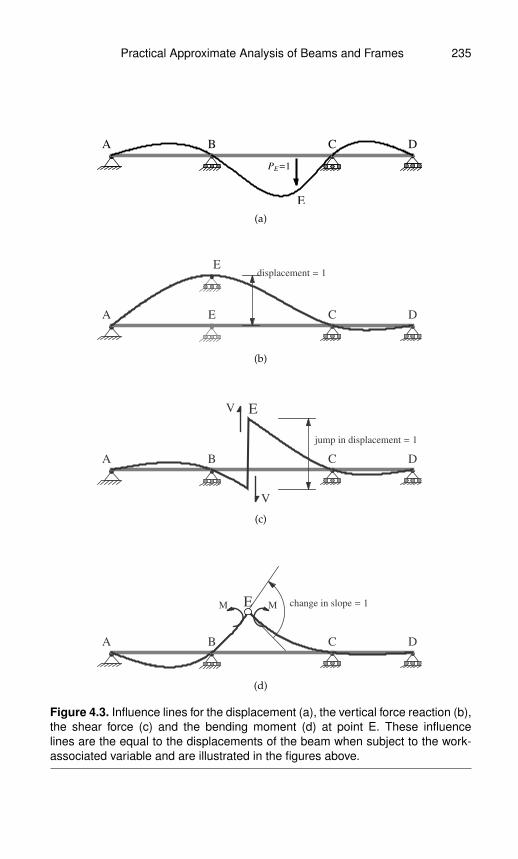
Practical Approximate Analysis of Beams and Frames 235
PE=1
A B C D
E
(a)
E
A E C D
displacement = 1
(b)
E
A B C D
jump in displacement = 1
V
V
(c)
change in slope = 1M ME
A B C D
(d)
Figure 4.3. Influence lines for the displacement (a), the vertical force reaction (b),the shear force (c) and the bending moment (d) at point E. These influencelines are the equal to the displacements of the beam when subject to the work-associated variable and are illustrated in the figures above.

236 Practical Approximate Analysis of Beams and Frames
the unit work-associated variable at point E. Specifically, we note thefollowing:
• For the influence line of the vertical reaction (see figure 4.3b), a unitdisplacement is applied at the support with an associated unknownreaction force. In particular, we do not apply an external point momentat point E unless it also happens to have a fixed support.
• For the influence line of the shear force (see figure 4.3c), a unit jumpin the displacement is applied with an associated unknown equal andopposite forces ‘V .’ This unit jump causes a discontinuity in the beam,but the slope before and after point E must be the same. In addition,there is an internal bending moment at point E. Also note that the jumpin displacement must be up when going from the left to the right of thebeam at point E and is implied by the shear force convention used inthis book. In addition, the individual displacements before and afterpoint E are unknown (ie. only the jump is known) and must be calcu-lated using structural analysis.
• For the influence line of the bending moment (see figure 4.3d), a unitchange in the slope is applied with associated unknown equal and op-posite moments ‘M .’ This unit change in slope causes a discontinuityin the slope of the beam but there is no discontinuity in the displace-ment. In addition, there is an internal shear force at point E. Also notethat the change in slope must be clockwise as shown in the figure whengoing from the left to the right of the beam at point E and is basedon the bending moment convention used in this book. In addition,the individual slopes before and after point E are unknown (ie. onlythe change in slope is known) and must be calculated using structuralanalysis.
In the next sections, we will use the Muller-Breslau principle to con-struct influence lines for both statically determinate and statically inde-terminate structures. The principle applies to both cases, but for staticallydeterminate structures, we can always manually construct the exact in-fluence line. In the case of statically indeterminate structures, we willdescribe methods to sketch an approximation to the influence lines withapproximate values calculated at notable points such as the maximumand minimum values in each span.
Using the Muller-Breslau principle we can identify rules for con-structing influence lines for both statically determinate and statically in-determinate structures in the case of force reactions, shear forces andbending moments. Some of these rules are specific for the consideredresponse variable and some are common. The common rules are as fol-lows:
Practical Approximate Analysis of Beams and Frames 237
1. The influence line passes through zero at all supports except for onecase. That case occurs only at one support on the beam and onlywhen we consider the influence line for the force reaction at that sup-port. In that case, that particular support moves up by one unit (eg.figure 4.3b).
2. The influence line is continuous (ie. no step jumps) except for onecase. That case occurs only at one location on the beam and onlywhen we consider the influence line for the shear force at that loca-tion. In that case, the discontinuity is a unit step jump at that location(eg. figure 4.3c).
3. The influence line away from internal hinges is smooth (ie. continuousslope) except for one case. That case occurs only at one location on thebeam and only when we consider the influence line for the bendingmoment at that location. In that case, there is a sudden change in slopeof one unit at that location (eg. figure 4.3d). Of course, there may bechanges in slopes at internal hinges.
In addition to the above rules, we have a rule that applies to all stat-ically stable beams, specifically:
4. The influence line for statically stable beams is piecwise smooth. Theinfluence line is then a sequence of possibly distinct smooth lines(ie. derivative is continuous) with possible step jumps and suddenchanges in direction between segments as outlined in the previousrules.
In addition to the above rules, we have one additional rule that is aspecial case of rule (4) above but only applies to statically determinatebeams, specifically:
5. For statically determinate beams, the influence line is piecwise linear.The influence line is then a sequence of possibly distinct straight lineswith possible step jumps and sudden changes in direction betweensegments as outlined in the previous rules.
It is this last rule that allows us to relatively easily construct the ex-act influence lines for statically determinate beams in the case of forcereactions, shear forces and bending moments. Further details and exam-ples for constructing the influence lines of statically determinate beamsis considered next.

238 Practical Approximate Analysis of Beams and Frames
4.2 Exact Influence Lines for StaticallyDeterminate Beams
4.2.1 Introduction to Sketching the Influence Linefor Statically Determinate Beams
For statically determinate beams, it is relatively easy to construct the ex-act influence lines for reactions, shear forces and bending moments usingthe few simple rules considered above. However, we must first verifythat we are indeed trying to analyze a statically determinate beam be-fore using those rules. The simplest statically determinate beams haveeither a hinge and a roller support or have one fixed end (eg. see beamsin figures 4.4). If we add a roller support or a fixed support to a staticallydeterminate beam then we must also add one or two internal hinges re-spectively or some equivalent internal constraints in order to maintainthe statical determinancy. Of course, as we add internal hinges, we mustbe careful to maintain statical stability.
For our purposes in this section, we only need statical determinancyas related to shear forces and bending moments. This means that, for thecases considered in this section, we must be able to fully determine shearforces and bending moments based on the equations of statics alone. In-determinancy with respect to axial forces is immaterial to the discussionsof this section. Therefore, the rules for constructing influence lines re-main the same as those of statically determinate beams if one or morehinge supports are replaced with a horizontal roller as long as there re-mains at least one reaction in the horizontal direction on the beam torestrict horizontal translations.
In what follows, we will present examples and discuss them in or-der to clarify how the identified rules may be used to construct influ-ence lines. Note however that the examples considered are extensive butnot comprehensive of all possible configurations. The examples progressfrom having no internal hinges to having one then two internal hinges.
4.2.2 Sketching Influence Lines for VerticalForce Reactions
In the first examples of the influence lines for vertical reaction forces, weconsider statically determinate beams with no internal hinges as shownin figure 4.4a and b. In such cases, the influence line for a vertical reactionforce is a single straight line. When there is a hinge and roller support,the influence line has a value of one at the support considered and passesthrough zero at the other support. Using the equation of a straight line orequivalently using similar triangles, we can then determine the value of
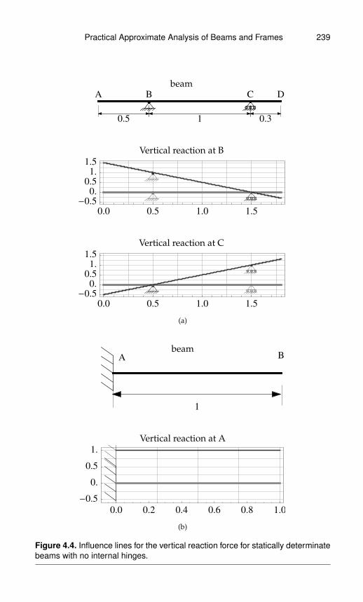
Practical Approximate Analysis of Beams and Frames 239
beam
0.5 1 0.3
A B C D
Vertical reaction at B
0.0 0.5 1.0 1.5
-0.5
0.
0.5
1.
1.5
Vertical reaction at C
0.0 0.5 1.0 1.5
-0.5
0.
0.5
1.
1.5
(a)
beam
1
A B
Vertical reaction at A
0.0 0.2 0.4 0.6 0.8 1.0
-0.5
0.
0.5
1.
(b)
Figure 4.4. Influence lines for the vertical reaction force for statically determinatebeams with no internal hinges.
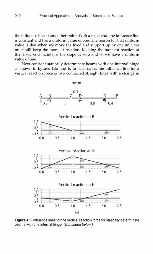
240 Practical Approximate Analysis of Beams and Frames
the influence line at any other point. With a fixed end, the influence lineis constant and has a uniform value of one. The reason for that uniformvalue is that when we move the fixed end support up by one unit, wemust still keep the moment reaction. Keeping the moment reaction atthat fixed end maintains the slope at zero and so we have a uniformvalue of one.
Next consider statically determinate beams with one internal hingeas shown in figures 4.5a and b. In such cases, the influence line for avertical reaction force is two connected straight lines with a change in
beam
0.3 1
0.3
0.8 0.4
A B C D E F
Vertical reaction at B
0.0 0.5 1.0 1.5 2.0 2.5
-0.50.
0.51.
1.5
Vertical reaction at D
0.0 0.5 1.0 1.5 2.0 2.5
-0.50.
0.51.
1.5
Vertical reaction at E
0.0 0.5 1.0 1.5 2.0 2.5
-0.50.
0.51.
1.5
(a)
Figure 4.5. Influence lines for the vertical reaction force for statically determinatebeams with one internal hinge. (Continued below.)
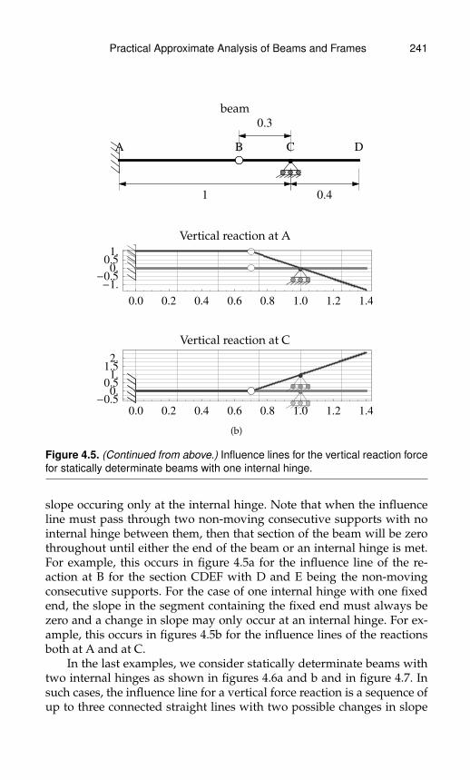
Practical Approximate Analysis of Beams and Frames 241
beam
1
0.3
0.4
A B C D
Vertical reaction at A
0.0 0.2 0.4 0.6 0.8 1.0 1.2 1.4
-1.-0.5
0.0.51.
Vertical reaction at C
0.0 0.2 0.4 0.6 0.8 1.0 1.2 1.4
-0.50.
0.51.
1.52.
(b)
Figure 4.5. (Continued from above.) Influence lines for the vertical reaction forcefor statically determinate beams with one internal hinge.
slope occuring only at the internal hinge. Note that when the influenceline must pass through two non-moving consecutive supports with nointernal hinge between them, then that section of the beam will be zerothroughout until either the end of the beam or an internal hinge is met.For example, this occurs in figure 4.5a for the influence line of the re-action at B for the section CDEF with D and E being the non-movingconsecutive supports. For the case of one internal hinge with one fixedend, the slope in the segment containing the fixed end must always bezero and a change in slope may only occur at an internal hinge. For ex-ample, this occurs in figures 4.5b for the influence lines of the reactionsboth at A and at C.
In the last examples, we consider statically determinate beams withtwo internal hinges as shown in figures 4.6a and b and in figure 4.7. Insuch cases, the influence line for a vertical force reaction is a sequence ofup to three connected straight lines with two possible changes in slope

242 Practical Approximate Analysis of Beams and Frames
beam
0.15 0.5
0.2
0.8
0.24
0.7 0.1
A B C D E F G H
Vertical reaction at B
0.0 0.5 1.0 1.5 2.0-1.5
-1.
-0.5
0.
0.5
1.
1.5
Vertical reaction at D
0.0 0.5 1.0 1.5 2.0-1.5
-1.
-0.5
0.
0.5
1.
1.5
Vertical reaction at F
0.0 0.5 1.0 1.5 2.0-1.5
-1.
-0.5
0.
0.5
1.
1.5
Vertical reaction at G
0.0 0.5 1.0 1.5 2.0-1.5
-1.
-0.5
0.
0.5
1.
1.5
(a)
Figure 4.6. Influence lines for the vertical reaction force for statically determinatebeams with two internal hinges and no fixed ends. (Continued below.)

Practical Approximate Analysis of Beams and Frames 243
beam
0.15 0.5
0.2
0.8 0.7
0.21
0.1
A B C D E F G H
Vertical reaction at B
0.0 0.5 1.0 1.5 2.0-1.5
-1.
-0.5
0.
0.5
1.
1.5
Vertical reaction at D
0.0 0.5 1.0 1.5 2.0-1.5
-1.
-0.5
0.
0.5
1.
1.5
Vertical reaction at E
0.0 0.5 1.0 1.5 2.0-1.5
-1.
-0.5
0.
0.5
1.
1.5
Vertical reaction at G
0.0 0.5 1.0 1.5 2.0-1.5
-1.
-0.5
0.
0.5
1.
1.5
(b)
Figure 4.6. (Continued from above.) Influence lines for the vertical reaction forcefor statically determinate beams with two internal hinges and no fixed ends.
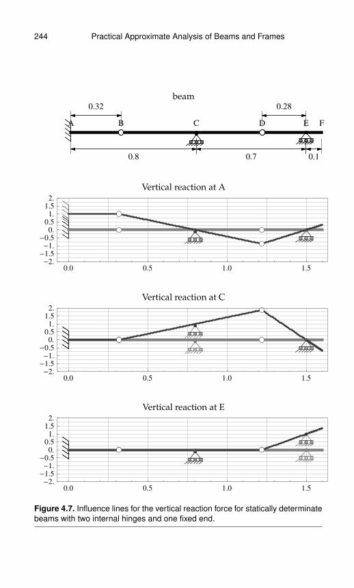
244 Practical Approximate Analysis of Beams and Frames
beam
0.8
0.32
0.7
0.28
0.1
A B C D E F
Vertical reaction at A
0.0 0.5 1.0 1.5-2.
-1.5
-1.
-0.5
0.
0.5
1.
1.5
2.
Vertical reaction at C
0.0 0.5 1.0 1.5-2.
-1.5
-1.
-0.5
0.
0.5
1.
1.5
2.
Vertical reaction at E
0.0 0.5 1.0 1.5-2.
-1.5
-1.
-0.5
0.
0.5
1.
1.5
2.
Figure 4.7. Influence lines for the vertical reaction force for statically determinatebeams with two internal hinges and one fixed end.
Practical Approximate Analysis of Beams and Frames 245
that may only occur at the two internal hinges. Figures 4.6a and b givestwo sets of examples of a beam having a hinge and two rollers with twointernal hinges while figure 4.7 gives a set of examples of a beam with afixed end and two rollers with two internal hinges.
In all cases of statically determinate beams without fixed ends, wecan first determine the values at all points of the line segment containingthe support that is moved up by a unit. In that line segment, we knowthe coordinates of two points which completely defines the equation ofthe straight line segment. For example, in figures 4.6a we first determinethe line segment ABC, CDE, EFGH and EFGH for the influence line ofthe reactions at B, D, F and G respectively. The first known coordinate inthose segments is the support being moved since its height is one unitand its horizontal position is known. For the second known coordinate,there are two possibilities. If there is a support adjacent to the supportbeing moved and such that there is no internal hinge between the twosupports then that adjacent support is the second coordinate with heightzero. That adjacent support must be connected by a straight line to thesupport being moved because slope changes may only occur at inter-nal hinges and it must have a height of zero because it is a support. Forexample, in figures 4.6a for the influence lines of the reaction at F, thenearest support with no internal hinge in-between is support G and forthe reaction at G, the nearest support with no internal hinge in-betweenis support F. Similarly in figures 4.6b, the influence line for the reactionat D, the moving support D has the nearest support point E with no in-ternal hinge in-between. Also in figure 4.6b, for the influence line for thereaction at E, the moving support E has the nearest support point D withno internal hinge in-between. All those adjacent supports with no inter-nal hinge in-between them and the moving support have zero height andare connected to the moving support by a straight line segment as shownin the corresponding figures.
In the second possiblity, we have either a free end or an internalhinge on either side of the support being moved by one unit. If thereis one adjacent free end and one adjacent internal hinge then the inter-nal hinge must have zero height otherwise the beam is statically unsta-ble. For example, in figure 4.6a with the influence line for the reactionat B, one side of the moving support B is free (point A) and the other isan internal hinge (point C). Therefore, the internal hinge (point C) musthave zero height. A similar situation occurs in the examples for the in-fluence lines for the vertical reactions at B and at G in figures 4.6b. Ifthe two adjacent ends have internal hinges then one and only one ofthose internal hinges must have zero height. The one internal hinge withthe zero height is determined by considering the kinematics of the restof the beam. In figure 4.6b with the influence line for the reaction at D,
246 Practical Approximate Analysis of Beams and Frames
both sides of the moving support D are internal hinges (points C and E).Due to kinematic constraints on the right side of the beam, the right-side internal hinge (point E) must have zero height. The kinematic con-straint on the right consists of two adjacent supports with no internalhinge between them and this necessarily means that the beam remainsat zero over that segment until an internal hinge or a free end is met ateither end.
In the case when we have a fixed end in a beam with two or moreinternal hinges, then we consider two cases. First, if the fixed supportmoves up by one unit then the line segment from that fixed support tothe nearest internal hinge must have a uniform value of one. The near-est internal hinge must be nearer to the fixed end than the next supportotherwise the beam will not be statically determinate. In the second case,if a roller moves up by one unit then the case is similar to having onlyhinges and rollers as supports with the added condition that the internalhinge nearest to a fixed end always has a height of zero. The reason forthe zero height is that the fixed end must have zero slope and zero heightand that the fixed end and nearest internal hinge must be connected bya straight line. Those two condition imply a straight line between themthat is uniformly zero.
In all cases, once the first line segment has been constructed, the restof the line segments are similarly determined by starting at the endsof a known line segment whose coordinates have already been foundand determining the equations of the adjacent segments. Those adjacentsegments are similarly determined by the coordinates of the known endpoints and the coordinates of the next adjacent support with no internalhinges in between. If an internal hinge occurs before then next adjacentsupport then that internal hinge must have zero height otherwise thebeam is statically unstable. In all cases, the coordinates of adjacent linesegments are determined until the influence line of the whole beam isconstructed.
4.2.3 Sketching Influence Lines for Shear Forces
The influence lines for shear forces look similar to those of the verticalforce reactions except for the distinctive unit step jump at the monitoredlocation. For example, figure 4.8 shows the influence line for the shearforce at point P with the distinctive unit step jump. The jump belowand above zero at point P in figure 4.8 may be determined based on thefollowing conditions: i) the total jump has a value of one and ii) the slopejust before and just after the jump must be the same. Using these twoconditions and the fact that the influence line for a statically determinate

Practical Approximate Analysis of Beams and Frames 247
Vbottom
Vtop
xP=LleftLright
L
P
Figure 4.8. Influence line for the shear force at point P shows the distinctive unitstep jump at point P . The jump below and above zero (ie. Vbottom and Vtop) maybe computed using simple equations.
beam is piecewise linear, we get the following equations:
Vbottom + Vtop = 1 (4.3a)Vbottom/Lleft = Vtop/Lright (4.3b)
⇒ Vbottom =Lleft
L=xPL
(4.3c)
Vtop =Lright
L= 1− xP
L(4.3d)
where:
Vbottom and Vtop are the values of the influence line just before and justafter point P respectively
Lleft and Lright are the distances between the left support and point Pand between point P and the right support respectively
L is the length of the span containing point P
point P is the point at which we are calculating the influence line forshear
xP is the abscissa (ie. x-coordinate) of point P when the origin is takenat the left support of the span containing P
Note that the value of the influence line at just before point P de-pends on the distance of point P from the left support. This value, de-noted by Vbottom in figure 4.8, varies linearly with the location of point P(ie. with xP ) as that location varies from being at the left support to beingat the right. Specifically, Vbottom is zero when point P is at the left supportand is one when point P is at the right support. The influence line at
248 Practical Approximate Analysis of Beams and Frames
just after point P also varies linearly with location but starts at one atthe left support and ends at zero at the right support. Once the values ofthe influence line at just before and at just after point P are determined,we then use the same approach that we used for the influence lines forvertical force reactions to construct the influence line for the shear force.In what follows are examples that further clarify such a construction.
In the first examples of the influence lines for shear forces, we con-sider statically determinate beams with no internal hinges as shown infigure 4.9a and b. In such cases, the influence line for a shear force con-sists of two consecutive straight line segments having the same slope andwith a unit discontinuity between them. Whenever the point of influenceis within an overhang (ie. a segment with a free end), the influence line isuniform from the free end up to the point at which influence is calculatedand then the rest of the influence line is identically zero. In these casesof the point of influence occuring in an overhang, the uniformity or zeroslope of the influence line is required to maintain slope continuity in thebeam before and after the point of influence. For example, in figure 4.9a,the influence line for the shear force at B is minus one in segment AB andzero for the rest of the beam. In this case, the shear force must be nega-tive in the left portion AB because the unit step jump condition requiresa step up going left to right and the right part of the beam must remain atzero due to having two consecutive supports with no internal hinge be-tween them. By contrast, in figure 4.9a for the influence line for the shearforce at F and in figure 4.9b for the influence line for the shear force at B,the left side of the beam before the point of influence is zero and the restis at positive one. This is again due to constraints imposed by the sup-ports on the left side of the beam and the requirement of stepping up byone unit from left to right at the point of influence. Finally, a case whenwe need to calculate the influence between a hinge and a roller is shownin figure 4.9a for the influence line for the shear force at D. The value ofthe influence line just before and just after point D is calculated usingformulas 4.3c and d and the rest of the beam is constructed in a mannersimilar to that described in the section for vertical force reactions.
Next consider statically determinate beams with one internal hingeas shown in figures 4.10a and b. In such cases, the influence line for theshear force is up to three connected straight lines with a change in slopeoccuring only at the internal hinge. Again when the influence line mustpass through two non-moving consecutive supports with no internalhinge between them, then that section of the beam will be zero through-out until either the end of the beam or an internal hinge is met. For ex-ample, this occurs in figure 4.10a for the influence line of the shear forceat D. As for the case of the influence line for the shear force in an over-hang segment, a beam with any number of internal hinges is handled

Practical Approximate Analysis of Beams and Frames 249
beam
0.5
0.2
1
0.3
0.3
0.15
A B C D E F G
Shear force at B
0.0 0.5 1.0 1.5
-1.
-0.5
0.
0.5
1.
Shear force at D
0.0 0.5 1.0 1.5
-1.
-0.5
0.
0.5
1.
Shear force at F
0.0 0.5 1.0 1.5
-1.
-0.5
0.
0.5
1.
(a)
Figure 4.9. Influence lines for the shear force for statically determinate beamswith no internal hinges. (Continued below.)
exactly as before irrespective of the presence of the internal hinge. Ofcourse, an internal hinge may not occur in an overhang to avoid staticalinstability.
Next we consider statically determinate beams with two internalhinges as shown in figures 4.11 and in figure 4.12. In such cases, the influ-ence line for a shear force is a sequence of up to four connected straight

250 Practical Approximate Analysis of Beams and Frames
beam
1
0.4
A B C
Shear force at B
0.0 0.2 0.4 0.6 0.8 1.0
-1.
-0.5
0.
0.5
1.
(b)
Figure 4.9. (Continued from above.) Influence lines for the shear force for stati-cally determinate beams with no internal hinges.
lines with two possible changes in slope that may only occur at the twointernal hinges. Figures 4.11 gives two set of examples of a beam havinga hinge and two rollers with two internal hinges while figure 4.12 givesa set of examples of a beam with a fixed end and two rollers with twointernal hinges.
In one of those examples, specifically figure 4.12 for the shear forceat B, we consider the influence line for a point between a left-end fixedsupport and a roller support when the point monitored occurs to theleft of the internal hinge in that span. In that case, the influence line iszero from the support (ie. point A) to the point of influence (ie. point B)because the slope and value in that segment are constrained by thefixed end. The influence line then jumps up to one at the point of in-fluence (ie. point B) and maintains that uniform value of one until wereach the internal hinge (ie. point D). This jump is required based on theMuller-Breslau principle for shear forces and the uniform value impliesa zero slope which is required to match slopes before and after the jump.

Practical Approximate Analysis of Beams and Frames 251
beam
0.3
0.12
1
0.30.3
0.8
0.4
0.4
0.16
A B C D E F G H I J
Shear force at B
0.0 0.5 1.0 1.5 2.0 2.5
-1.-0.5
0.0.5
1.
Shear force at D
0.0 0.5 1.0 1.5 2.0 2.5
-1.-0.5
0.0.5
1.
Shear force at G
0.0 0.5 1.0 1.5 2.0 2.5
-1.-0.5
0.0.5
1.
Shear force at I
0.0 0.5 1.0 1.5 2.0 2.5
-1.-0.5
0.0.5
1.
(a)
Figure 4.10. Influence lines for the shear force for statically determinate beamswith one internal hinge. (Continued below.)

252 Practical Approximate Analysis of Beams and Frames
beam
1
0.3 0.3
0.4
0.2
A B C D E F
Shear force at C
0.0 0.2 0.4 0.6 0.8 1.0 1.2 1.4
-1.
-0.5
0.
0.5
1.
Shear force at E
0.0 0.2 0.4 0.6 0.8 1.0 1.2 1.4
-1.
-0.5
0.
0.5
1.
(b)
Figure 4.10. (Continued from above.) Influence lines for the shear force for stati-cally determinate beams with one internal hinge.
Finally, at the internal hinge (ie. point C), the influence line changes di-rection in order to meet the roller support (ie. point D) at zero.
The previous case considered is to be contrasted with the case in asimilar span with a left-end fixed support but when the point of influ-ence occurs after the internal hinge such as in figure 4.10b for the shearforce at C. In that case, the influence line is zero until the internal hingewhich is again due to the fixed end constraints. At the internal hinge, theinfluence line changes direction downwards until we reach the point ofinfluence (ie. point C). At the point of influence (ie. point C), the influenceline jumps up by one unit as required by the Muller-Breslau principle forshear forces. Finally, the influence line then goes downwards again at thesame slope as before the jump in order to meet the roller support at zero.Note that, in this case, a change in direction downwards at the internal

Practical Approximate Analysis of Beams and Frames 253
beam
0.15
0.06
0.5
0.20.15
0.8
0.240.4
0.7
0.28
0.1
AB C D E F G H I J K L
Shear force at B
0.0 0.5 1.0 1.5 2.0
-1.
-0.5
0.
0.5
1.
Shear force at D
0.0 0.5 1.0 1.5 2.0
-1.
-0.5
0.
0.5
1.
Shear force at G
0.0 0.5 1.0 1.5 2.0
-1.
-0.5
0.
0.5
1.
Shear force at J
0.0 0.5 1.0 1.5 2.0
-1.
-0.5
0.
0.5
1.
Figure 4.11. Influence lines for the shear force for statically determinate beamswith two internal hinges and no fixed ends.
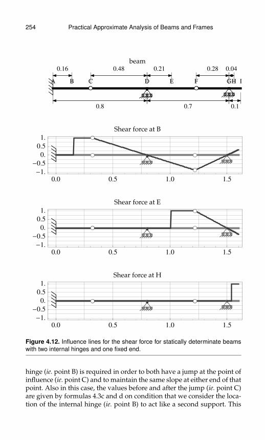
254 Practical Approximate Analysis of Beams and Frames
beam
0.8
0.480.16
0.7
0.280.21
0.1
0.04
A B C D E F GH I
Shear force at B
0.0 0.5 1.0 1.5
-1.
-0.5
0.
0.5
1.
Shear force at E
0.0 0.5 1.0 1.5
-1.
-0.5
0.
0.5
1.
Shear force at H
0.0 0.5 1.0 1.5
-1.
-0.5
0.
0.5
1.
Figure 4.12. Influence lines for the shear force for statically determinate beamswith two internal hinges and one fixed end.
hinge (ie. point B) is required in order to both have a jump at the point ofinfluence (ie. point C) and to maintain the same slope at either end of thatpoint. Also in this case, the values before and after the jump (ie. point C)are given by formulas 4.3c and d on condition that we consider the loca-tion of the internal hinge (ie. point B) to act like a second support. This

Practical Approximate Analysis of Beams and Frames 255
means that the effective span ‘L’ is considered to be the distance betweenthe internal hinge and the roller support (ie. distance between B and D).Cases when the fixed support is at the right are similar but with oppositesigns as those of fixed supports at the left that were discussed and maybe similarly reasoned and constructed.
Finally, we consider the special cases of influence lines for the shearforces at the location of supports, shown in the examples of figures 4.13aand b. In such cases, we must specify whether the point being monitoredis slightly to the left or slightly to the right of the support. If the supportis slightly to the left, as in figure 4.13a for the shear force at B−, then thevalue just before the support equals minus one in order to have a jump ofone from left to right and to reach zero at the support. By contrast, if thesupport is slightly to the right, as in figure 4.13a for the shear force at B+,then the value just after the support equals one in order to have a jumpof one from the support which must always be at zero. If the supportis at the left end of the beam, such as in figure 4.13b for the shear forceat A, then we can only consider the shear force slightly to the right ofthat support. In that case, the influence line for the shear force equals theinfluence line for the vertical reaction at the support because the reactionat that support equals the shear force slightly to the right of it when theforce is at any point to the right of that end point. The case for a supportat the right end of the beam is similar except that the influence line for theshear force is negative that of the vertical reaction force at that support.The reason has to do with the convention used to define negative andpositive shear forces in beams.
4.2.4 Sketching Influence Lines for Bending Moments
The influence lines for bending moments again look similar to those ofthe vertical force reactions except for the distinctive change of directionor kink at the monitored location. For example, figure 4.14 shows theinfluence line for the bending moment at point P with the distinctivekink. The value of the influence line at point P in figure 4.14 may bedetermined based on the following conditions: i) the total change in an-gle has a value of one at the kink and ii) the influence line is continuousat P . Using these two conditions and the fact that the influence line fora statically determinate beam is piecewise linear, we get the followingequation:
(Mat influence/Lleft) +(Mat influence/Lright
)= 1 (4.4a)
⇒ Mat influence =Lleft × Lright
L= xP
L
(1− xP
L
)L (4.4b)

256 Practical Approximate Analysis of Beams and Frames
beam
1 1 0.3
A B C D
Shear force at B−
0.0 0.5 1.0 1.5 2.0
-1.
-0.5
0.
0.5
1.
Shear force at B+
0.0 0.5 1.0 1.5 2.0
-1.
-0.5
0.
0.5
1.
(a)
beam
1 1
0.3
0.3
A B C D E
Shear force at A
0.0 0.5 1.0 1.5 2.0
-1.
-0.5
0.
0.5
1.
(b)
Figure 4.13. Influence lines for the shear force for statically determinate beamsnear supports.
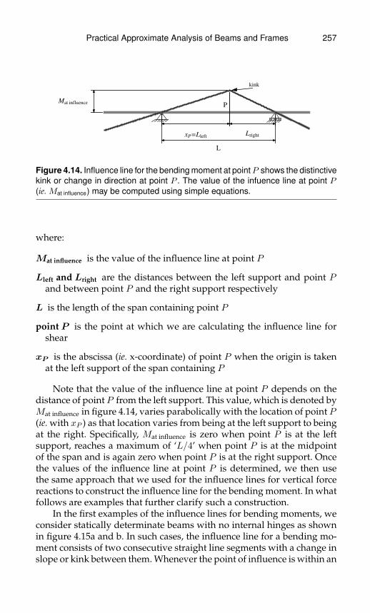
Practical Approximate Analysis of Beams and Frames 257
Mat influence
xP=LleftLright
L
kink
P
Figure 4.14. Influence line for the bending moment at pointP shows the distinctivekink or change in direction at point P . The value of the infuence line at point P(ie. Mat influence) may be computed using simple equations.
where:
Mat influence is the value of the influence line at point P
Lleft and Lright are the distances between the left support and point Pand between point P and the right support respectively
L is the length of the span containing point P
point P is the point at which we are calculating the influence line forshear
xP is the abscissa (ie. x-coordinate) of point P when the origin is takenat the left support of the span containing P
Note that the value of the influence line at point P depends on thedistance of point P from the left support. This value, which is denoted byMat influence in figure 4.14, varies parabolically with the location of point P(ie. with xP ) as that location varies from being at the left support to beingat the right. Specifically, Mat influence is zero when point P is at the leftsupport, reaches a maximum of ‘L/4’ when point P is at the midpointof the span and is again zero when point P is at the right support. Oncethe values of the influence line at point P is determined, we then usethe same approach that we used for the influence lines for vertical forcereactions to construct the influence line for the bending moment. In whatfollows are examples that further clarify such a construction.
In the first examples of the influence lines for bending moments, weconsider statically determinate beams with no internal hinges as shownin figure 4.15a and b. In such cases, the influence line for a bending mo-ment consists of two consecutive straight line segments with a change inslope or kink between them. Whenever the point of influence is within an
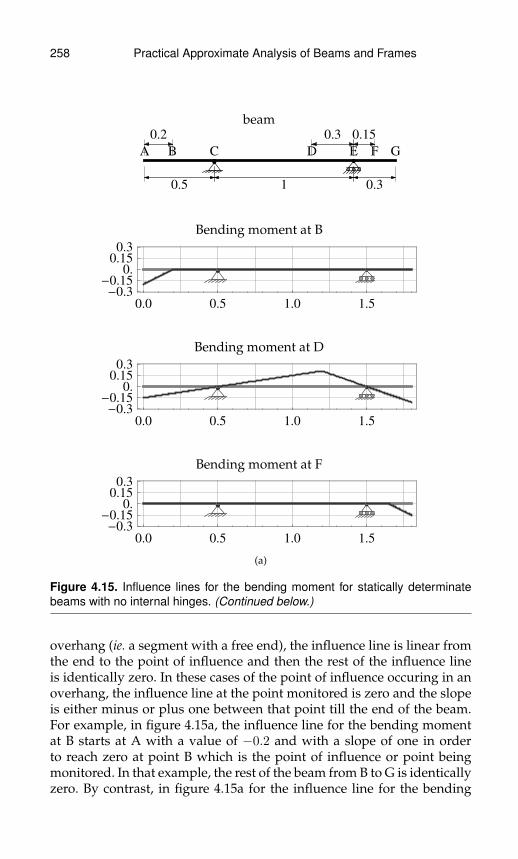
258 Practical Approximate Analysis of Beams and Frames
beam
0.5
0.2
1
0.3
0.3
0.15
A B C D E F G
Bending moment at B
0.0 0.5 1.0 1.5
-0.3-0.15
0.0.15
0.3
Bending moment at D
0.0 0.5 1.0 1.5
-0.3-0.15
0.0.15
0.3
Bending moment at F
0.0 0.5 1.0 1.5
-0.3-0.15
0.0.15
0.3
(a)
Figure 4.15. Influence lines for the bending moment for statically determinatebeams with no internal hinges. (Continued below.)
overhang (ie. a segment with a free end), the influence line is linear fromthe end to the point of influence and then the rest of the influence lineis identically zero. In these cases of the point of influence occuring in anoverhang, the influence line at the point monitored is zero and the slopeis either minus or plus one between that point till the end of the beam.For example, in figure 4.15a, the influence line for the bending momentat B starts at A with a value of −0.2 and with a slope of one in orderto reach zero at point B which is the point of influence or point beingmonitored. In that example, the rest of the beam from B to G is identicallyzero. By contrast, in figure 4.15a for the influence line for the bending

Practical Approximate Analysis of Beams and Frames 259
beam
1
0.4
A B C
Bending moment at B
0.0 0.2 0.4 0.6 0.8 1.0
-0.6-0.45-0.3-0.15
0.0.15
0.30.45
0.6
(b)
Figure 4.15. (Continued from above.) Influence lines for the bending moment forstatically determinate beams with no internal hinges.
moment at F and in figure 4.9b for the influence line for the bendingmoment at B, the left side of the beam before the point of influence iszero and the rest is a straight line with slope minus one and a value ofzero at the point of influence. Finally, a case when we need to calculatethe influence between a hinge and a roller is show in figure 4.15a for theinfluence line for the bending moment at D. The value of the influenceline at point D is calculated using formula 4.4b and the rest of the beamis constructed in a manner similar to that described in the section forvertical force reactions.
Next consider statically determinate beams with one internal hingeas shown in figures 4.16a and b. In such cases, the influence line for thebending moment is up to three connected straight lines with a changein slope occuring in the internal hinge and a unit change in slope occur-ing at the point of influence. Again when the influence line must passthrough two non-moving consecutive supports with no internal hingebetween them, then that section of the beam will be zero throughout
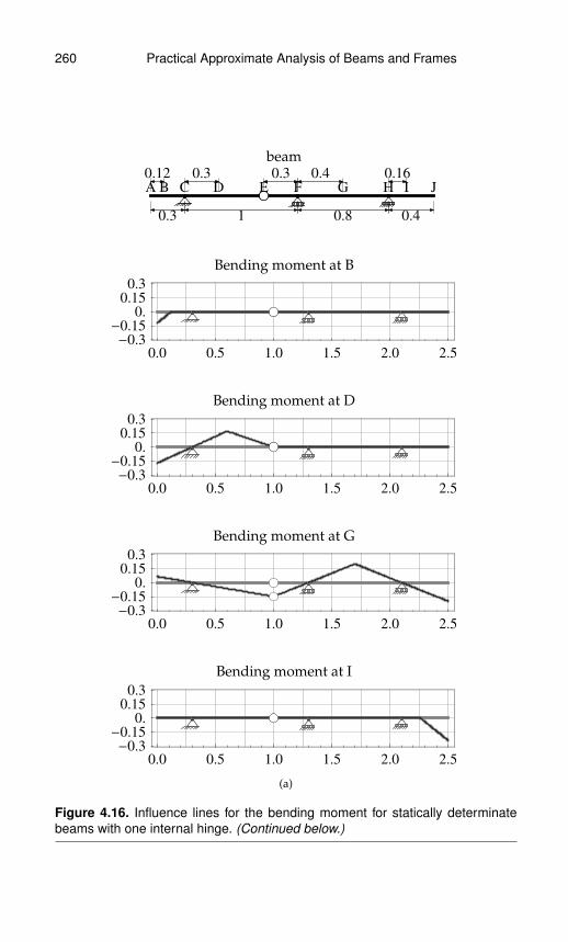
260 Practical Approximate Analysis of Beams and Frames
beam
0.3
0.12
1
0.30.3
0.8
0.4
0.4
0.16
A B C D E F G H I J
Bending moment at B
0.0 0.5 1.0 1.5 2.0 2.5
-0.3
-0.15
0.
0.15
0.3
Bending moment at D
0.0 0.5 1.0 1.5 2.0 2.5
-0.3
-0.15
0.
0.15
0.3
Bending moment at G
0.0 0.5 1.0 1.5 2.0 2.5
-0.3
-0.15
0.
0.15
0.3
Bending moment at I
0.0 0.5 1.0 1.5 2.0 2.5
-0.3
-0.15
0.
0.15
0.3
(a)
Figure 4.16. Influence lines for the bending moment for statically determinatebeams with one internal hinge. (Continued below.)

Practical Approximate Analysis of Beams and Frames 261
beam
1
0.3 0.3
0.4
0.2
A B C D E F
Bending moment at C
0.0 0.2 0.4 0.6 0.8 1.0 1.2 1.4
-0.3
-0.15
0.
0.15
0.3
Bending moment at E
0.0 0.2 0.4 0.6 0.8 1.0 1.2 1.4
-0.3
-0.15
0.
0.15
0.3
(b)
Figure 4.16. (Continued from above.) Influence lines for the bending moment forstatically determinate beams with one internal hinge.
until either the end of the beam or an internal hinge is met. For example,this occurs in figure 4.16a for the influence line of the bending momentat D. The cases when we consider the influence line for the bending mo-ment in an overhang part of a beam, we handle it the same as for theexamples of figure 4.15 irrespective of the number internal hinges in therest of the beam. Of course, as before, an internal hinge may not occur inan overhang to avoid statical instability.
Next we consider statically determinate beams with two internalhinges as shown in figures 4.18 and in figure 4.19. In such cases, the in-fluence line for a bending moment is a sequence of up to four connectedstraight lines with two possible changes in slope that may occur at thetwo internal hinges and one mandatory unit change in slope that mustoccur at the point of influence. Figures 4.18 gives two set of examples ofa beam having a hinge and two rollers with two internal hinges while
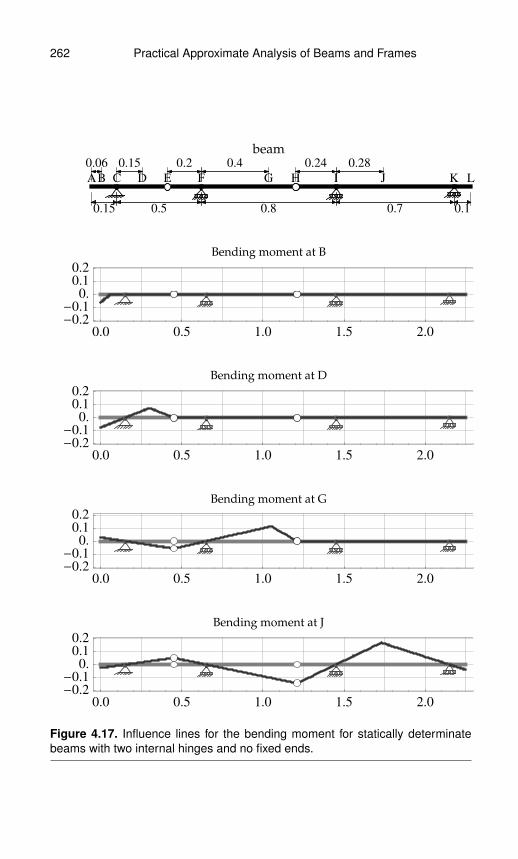
262 Practical Approximate Analysis of Beams and Frames
beam
0.15
0.06
0.5
0.20.15
0.8
0.240.4
0.7
0.28
0.1
AB C D E F G H I J K L
Bending moment at B
0.0 0.5 1.0 1.5 2.0
-0.2
-0.1
0.
0.1
0.2
Bending moment at D
0.0 0.5 1.0 1.5 2.0
-0.2
-0.1
0.
0.1
0.2
Bending moment at G
0.0 0.5 1.0 1.5 2.0
-0.2
-0.1
0.
0.1
0.2
Bending moment at J
0.0 0.5 1.0 1.5 2.0
-0.2
-0.1
0.
0.1
0.2
Figure 4.17. Influence lines for the bending moment for statically determinatebeams with two internal hinges and no fixed ends.
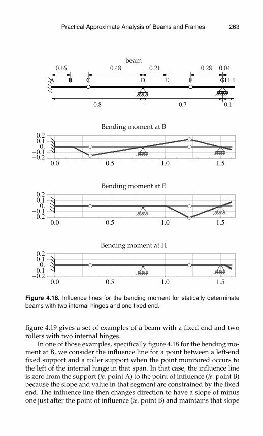
Practical Approximate Analysis of Beams and Frames 263
beam
0.8
0.480.16
0.7
0.280.21
0.1
0.04
A B C D E F GH I
Bending moment at B
0.0 0.5 1.0 1.5
-0.2-0.1
0.0.10.2
Bending moment at E
0.0 0.5 1.0 1.5
-0.2-0.1
0.0.10.2
Bending moment at H
0.0 0.5 1.0 1.5
-0.2-0.1
0.0.10.2
Figure 4.18. Influence lines for the bending moment for statically determinatebeams with two internal hinges and one fixed end.
figure 4.19 gives a set of examples of a beam with a fixed end and tworollers with two internal hinges.
In one of those examples, specifically figure 4.18 for the bending mo-ment at B, we consider the influence line for a point between a left-endfixed support and a roller support when the point monitored occurs tothe left of the internal hinge in that span. In that case, the influence lineis zero from the support (ie. point A) to the point of influence (ie. point B)because the slope and value in that segment are constrained by the fixedend. The influence line then changes direction to have a slope of minusone just after the point of influence (ie. point B) and maintains that slope

264 Practical Approximate Analysis of Beams and Frames
beam
1 1 0.3
A B C D
Bending moment at B−
0.0 0.5 1.0 1.5 2.0
-1.
-0.5
0.
Bending moment at B+
0.0 0.5 1.0 1.5 2.0
-1.
-0.5
0.
(a)
beam
1
0.3
1
0.2
0.3
A B C D E F
Bending moment at A
0.0 0.5 1.0 1.5 2.0
-1.
-0.5
0.
0.5
1.
(b)
Figure 4.19. Influence lines for the bending moment for statically determinatebeams near supports.
Practical Approximate Analysis of Beams and Frames 265
until we reach the internal hinge (ie. point D). The resulting net change indirection of one at the point of influence (ie. point B) is required based onthe Muller-Breslau principle for bending moments. Finally, at the inter-nal hinge (ie. point C), the influence line changes direction again in orderto meet the roller support (ie. point D) at zero.
The previous case considered is to be contrasted with the case in asimilar span with a left-end fixed support but when the point of influenceoccurs after the internal hinge such as in figure 4.16b for the bending mo-ment at C. In that case, the influence line is zero until the internal hingewhich is again due to the fixed end constraints. At the internal hinge,the influence line changes direction upwards until we reach the point ofinfluence (ie. point C). At the point of influence (ie. point C), the influ-ence line changes slope by one unit as required by the Muller-Breslauprinciple for bending moments. Finally, with the change in direction, theinfluence line then goes downwards to meet the roller support at zero.Note that, in this case, a change in direction upwards at the internal hinge(ie. point B) is required in order to both have a unit change in slope at thepoint of influence (ie. point C) and to subsequently meet the next support(ie. point D) at zero. Also in this case, the value at the point of influence(ie. point C) is given by formula 4.4b on condition that we consider thelocation of the internal hinge (ie. point B) to act like a second support.This means that the effective span ‘L’ is considered to be the distancebetween the internal hinge and the roller support (ie. distance between Band D). Cases when the fixed support is at the right are similar but withopposite signs as those of fixed supports at the left that were discussedand may be similarly reasoned and constructed.
Finally, we consider the special cases of influence lines for the bend-ing moments at the location of supports as shown in the examples offigures 4.19a and b. In such cases, and unlike the influence line for shearforces, there is no difference whether the point of influence is slightly tothe left or slightly to the right of the support. In either case, as in fig-ures 4.19a for the bending moments at B− and at B+, the only novelfeature is that the influence line at the point of influence must be zero atthe support. If the support is a hinge or roller that is at neither end ofthe beam, then this will imply, for statically determinate beams, that theslope is zero at one side of the point of influence and the slope is plusor minus one at the other side depending on whether this slope occursbefore or after the support respectively.
If we consider the influence line for the bending moment at a sup-port and that support is at either end of a statically determinate beamthen we have two cases. If the end support is a hinge or roller, then theinfluence line for the bending moment is identically zero throughout thewhole beam. This may be simply understood by noting that the bending

266 Practical Approximate Analysis of Beams and Frames
moment at a free hinge or roller support at either end of a beam must bezero irrespective of any loads applied within the beam. The second caseconsidered is when the end support is a fixed end. In that case, we canbetter understand the construction of the influence line if we consider thepoint of influence to be a small distance away from the fixed end. Thiscase is then similar to figure 4.18 for the bending moment at B but withpoint B being much close to point A. In the limit as the point of influencetends towards the fixed end (eg. point B tends to point A in figure 4.18for the bending moment at B), the horizontal line segment between thefixed support and the point of influence is omitted and we get an imme-diate change in slope of one at the fixed end as shown in figure 4.19b forthe bending moment at A. Incidentally, this influence line for the bend-ing moment at the fixed support must be the same as the influence linefor the moment reaction at the fixed support except for sign (ie. positiveor negative) which depend on the chosen sign convention for bendingmoments and moment reactions.
4.3 Approximate Influence Lines forStatically Indeterminate Structures
4.3.1 Introduction to Sketching the Influence Linefor Statically Indeterminate Beams
In the introduction to influence lines, we detailed rules for constructingthe influence lines for statically determinate and indeterminate beamsusing the Muller-Breslau principle. Based on that principle, sketching aninfluence line is equivalent to sketching the deformed shape for a spe-cific type of loading. The three types of loading of primary interest areshown in figures 4.3b, c and d which are used to obtain the influencelines for the vertical support reactions, the shear forces and the bendingmoments respectively. Under these types of loading, the deformations ofstatically determinate beams are piecewise linear while those for indeter-minate ones are, in general, piecewise cubic. In addition, the magnitudesand shapes of the deformed statically indeterminate beams depend onthe cross-sectional properties as well as on the length of the spans. Alsoin these cases, exact calculation of the deformed shape requires exactlysolving statically indeterminate beams subject to the associated load-ings. Since such solutions are, in general, complex and better suited forcomputer implementations, we will develop approximate approaches tosketch the deformations due to the special type of loadings identified infigures 4.3b, c and d which then gives approximate influence lines for thestatically indeterminate beams.
Practical Approximate Analysis of Beams and Frames 267
The approximate approach to sketch the deformation associatedwith a desired influence line is as follows:
1. Isolate the part in which the special type of loading is present andreplace the rest of the passive structure by rotary springs. In the caseof influence lines for shear forces and moments, the isolated part is justthe member that contains the point of influence. Figure 4.29a, b and cshow examples for the influence line for the bending moment whilefigure 4.26 shows an example for the influence line for the shear force.In the case of influence lines for vertical reaction forces, the isolatedpart depends on the location of the support. If the support is at eitherend then the isolated part is the member containing the support asshown, for example, in figures 4.20a and b. If the support is internal tothe beam then the isolated part are both members on either side of thesupport as shown, for example, in figure 4.23.
2. Analyze the deformation of the isolated part to obtain the approximatevalue and location of the maximum and minimum deformations inthat part. Also, obtain the rotations at both ends of that isolated part.
3. Based on known end rotations of the attached members, obtain theapproximate value and location of the maximum or minimum defor-mation as shown in figure 4.32. Also, obtain the rotation at the oppos-ing end of that member. With the new end rotations, this third step isrecursively used to obtain the deformations of all the rest of the mem-bers.
In what follows, we will do the following:
1. For each of the three types of influence lines identified in figures 4.3b,c and d, we will present an analysis of the isolated part. This includesdescribing how to sketch the deformed shape of the isolated part andto approximately identify maxima, minima and end rotations.
2. We will present and discuss the results needed to carry out the thirdstep above. This will apply to all types of influence lines for all mem-bers outside the isolated part.
3. Finally, for each of the three types of influence lines considered, wewill present examples and discuss them in order to clarify how the ob-tained results may be used to construct influence lines. Note howeverthat the examples considered are extensive but not comprehensive ofall possible configurations.
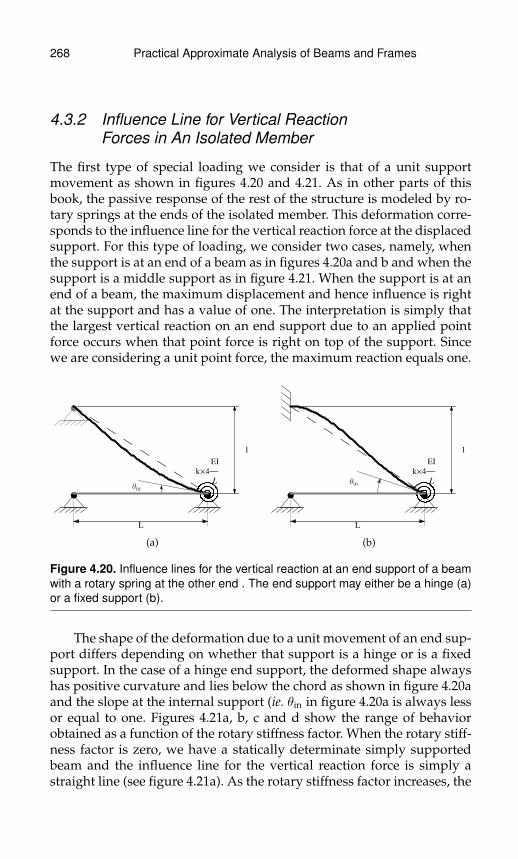
268 Practical Approximate Analysis of Beams and Frames
4.3.2 Influence Line for Vertical ReactionForces in An Isolated Member
The first type of special loading we consider is that of a unit supportmovement as shown in figures 4.20 and 4.21. As in other parts of thisbook, the passive response of the rest of the structure is modeled by ro-tary springs at the ends of the isolated member. This deformation corre-sponds to the influence line for the vertical reaction force at the displacedsupport. For this type of loading, we consider two cases, namely, whenthe support is at an end of a beam as in figures 4.20a and b and when thesupport is a middle support as in figure 4.21. When the support is at anend of a beam, the maximum displacement and hence influence is rightat the support and has a value of one. The interpretation is simply thatthe largest vertical reaction on an end support due to an applied pointforce occurs when that point force is right on top of the support. Sincewe are considering a unit point force, the maximum reaction equals one.
Θin
1
k´4
EI
L
L
(a)
Θin
1
k´4
EI
L
L
(b)
Figure 4.20. Influence lines for the vertical reaction at an end support of a beamwith a rotary spring at the other end . The end support may either be a hinge (a)or a fixed support (b).
The shape of the deformation due to a unit movement of an end sup-port differs depending on whether that support is a hinge or is a fixedsupport. In the case of a hinge end support, the deformed shape alwayshas positive curvature and lies below the chord as shown in figure 4.20aand the slope at the internal support (ie. θin in figure 4.20a is always lessor equal to one. Figures 4.21a, b, c and d show the range of behaviorobtained as a function of the rotary stiffness factor. When the rotary stiff-ness factor is zero, we have a statically determinate simply supportedbeam and the influence line for the vertical reaction force is simply astraight line (see figure 4.21a). As the rotary stiffness factor increases, the

Practical Approximate Analysis of Beams and Frames 269
Θin=1
1
L
1
0´4
EI
L
L
(a)
Θin=
3
7
1
L
1
1´4
EI
L
L
(b)
Θin=
1
5
1
L
1
3´4
EI
L
L
(c)
Θin=0
1
L
1
L
(d)
Figure 4.21. Influence lines for the vertical reaction at a hinge end support of abeam as the relative stiffness of the connected beam increases from zero (a) toone (b) to three (c) and to infinity which leads to a fixed end (d).
slope at the connected end decreases from 1/L to 0 where ‘L’ is the lengthof the span (see figures 4.21b, c and d).
By contrast with the hinge end support, when the end support isfixed then the deformed shape starts with negative curvature at thatend and, in general, ends with a positive curvature at the inner support.The exception is when the inner support is itself a hinge or roller, asshown in figure 4.22a where the deformed shape has a negative curva-ture throughout the beam. With a fixed end, the slope at the inner sup-port (ie. θin in figure 4.20b) is always less than 1.5/L. The inner slopeis exactly 1.5/L when the rotary stiffness factor equals zero as shownin figure 4.22a, and is exactly equal to 1/L and therefore tangent withthe chord, when the rotary stiffness factor equals half as shown in fig-ure 4.22b. When the rotary stiffness factor is greater than half then theinner slope is less than 1/L such as shown for a rotary stiffness factor ofone in figure 4.21c. In the limit of an infinite rotary stiffness factor andhence a fixed inner support, the slope is zero at the inner support.
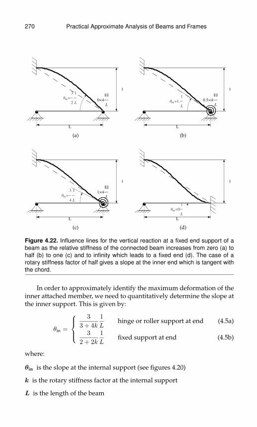
270 Practical Approximate Analysis of Beams and Frames
Θin=
3
2
1
L
1
0´4
EI
L
L
(a)
Θin=1.
1
L
1
0.5´4
EI
L
L
(b)
Θin=
3
4
1
L
1
1´4
EI
L
L
(c)
Θin=0
1
L
1
L
(d)
Figure 4.22. Influence lines for the vertical reaction at a fixed end support of abeam as the relative stiffness of the connected beam increases from zero (a) tohalf (b) to one (c) and to infinity which leads to a fixed end (d). The case of arotary stiffness factor of half gives a slope at the inner end which is tangent withthe chord.
In order to approximately identify the maximum deformation of theinner attached member, we need to quantitatively determine the slope atthe inner support. This is given by:
θin =
3
3 + 4k
1
Lhinge or roller support at end (4.5a)
3
2 + 2k
1
Lfixed support at end (4.5b)
where:
θin is the slope at the internal support (see figures 4.20)
k is the rotary stiffness factor at the internal support
L is the length of the beam
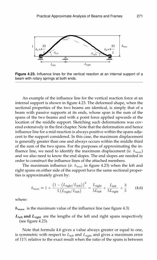
Practical Approximate Analysis of Beams and Frames 271
Θleft Θright
1 hmax
kL´4
EI
L
Lleft
kR´4
EI
L
Lright
Figure 4.23. Influence lines for the vertical reaction at an internal support of abeam with rotary springs at both ends.
An example of the influence line for the vertical reaction force at aninternal support is shown in figure 4.23. The deformed shape, when thesectional properties of the two beams are identical, is simply that of abeam with passive supports at its ends, whose span is the sum of thespans of the two beams and with a point force applied upwards at thelocation of the middle support. Sketching such deformations was cov-ered extensively in the first chapter. Note that the deformation and henceinfluence line for a mid-reaction is always positive within the spans adja-cent to the support considered. In this case, the maximum displacementis generally greater than one and always occurs within the middle thirdof the sum of the two spans. For the purposes of approximating the in-fluence line, we need to identify the maximum displacement (ie. hmax)and we also need to know the end slopes. The end slopes are needed inorder to construct the influence lines of the attached members.
The maximum influence (ie. hmax in figure 4.23) when the left andright spans on either side of the support have the same sectional proper-ties is approximately given by:
hmax ≈ 1 +
(1−
(Lright/Lleft
))25(Lright/Lleft
) =Lright
5Lleft+
Lleft
5Lright+
3
5(4.6)
where:
hmax is the maximum value of the influence line (see figure 4.3)
Lleft and Lright are the lengths of the left and right spans respectively(see figure 4.23).
Note that formula 4.6 gives a value always greater or equal to one,is symmetric with respect to Lleft and Lright and gives a maximum errorof 11% relative to the exact result when the ratio of the spans is between

272 Practical Approximate Analysis of Beams and Frames
half and two (ie. neither span is longer than twice the other). In that case,the exact value for the maximum possible influence equals about 1.23and occurs when one span is twice the other with the shorter span beingfixed and the longer span being hinged. This also happens to be the casewhere formula 4.6 has the largest errors relative to the exact results. Ingeneral, formula 4.6 is more accurate when the stiffness factors on bothsides (ie. kL and kR in figure 4.23) are both one or larger in which casethe maximum error is always less than 5% when the ratio of the spans isbetween half and two.
The other quantitative result we present for the case of the influenceline of the vertical reaction force at an internal support is that of the endslopes. Approximate expressions for those end slopes are given by:
θleft ≈3
4 + 4kL
(1
Lleft+
1
Lright
)(4.7a)
θright ≈3
4 + 4kR
(1
Lleft+
1
Lright
)(4.7b)
where:
θleft and θright are the slopes of the left and right ends respectively (seefigure 4.21)
Lleft and Lright are the lengths of the left and right spans respectively(see figure 4.21)
kL and kR are the rotary stiffness factors on the left and right respec-tively (see figure 4.21). Note that these stiffness factors are relative tothe left and right spans respectively which would be different than forthose of the two combined spans
Note that formulas 4.7a and b give a maximum possible error of 25%relative to the exact result when the ratio of the spans is between halfand two (ie. neither span is longer than twice the other). If in additionthe rotary stiffness factors on either side are larger than one then themaximum possible error is reduced to 10%.
In order to gain some familiarity with the shape of the influence linein this case, figures 4.24 and 4.25 provide some examples. In figures 4.24,the beams on either side of the inner support are equal. When both sidesare hinged, the resulting shape is shown in figure 4.24a. As the stiff-ness on either side increases, the slope decreases somewhat similar tothe cases shown for the fixed end support in figures 4.22. In each case,formula 4.6 may be used to estimate the end slopes and formula 4.7 maybe used to estimate the slopes at either end.

Practical Approximate Analysis of Beams and Frames 273
Θleft=1.50
1
L
Θright=1.50
1
L
1 hmax=1
0´4
EI
L
L
0´4
EI
L
L
(a)
Θleft=0.75
1
L
Θright=0.75
1
L
1 hmax=1
1´4
EI
L
L
1´4
EI
L
L
(b)
Θleft=0.78
1
L
Θright=0.36
1
L
1 hmax=1.00
1´4
EI
L
L
3´4
EI
L
L
(c)
Θleft=1.71
1
LΘright=0
1
L
1 hmax=1.02
0´4
EI
L
L L
(d)
Figure 4.24. Influence lines for the vertical reaction at an internal support of abeam with rotary springs at both ends. In all cases the beams on either sideof the inner support are equal with various combinations of the rotary stiffnessfactors at each end shown. Even when one side is fixed and the other hinged, themaximum displacement barely increases above one as shown in case (d).
Θleft=1.25
1
LΘright=1
1
L
1hmax=1.09
0´4
EI
L
L
0´4
EI
L
2L
(a)
Θleft=0.59
1
L
Θright=0.54
1
L
1hmax=1.10
1´4
EI
L
L
1´4
EI
L
2L
(b)
Θleft=0.60
1
L
Θright=0.26
1
L
1hmax=1.08
1´4
EI
L
L
3´4
EI
L
2L
(c)
Θleft=0
1
L
Θright=1.23
1
L
1
hmax=1.23
L
0´4
EI
L
2L
(d)
Figure 4.25. Influence lines for the vertical reaction at an internal support of abeam with rotary springs at both ends. In all cases the inner beam on the rightis twice that on the left with various combinations of the rotary stiffness factors ateach end shown.

274 Practical Approximate Analysis of Beams and Frames
In figures 4.25, the beams on the right are twice the length of thoseon the left. These figures shows the range of shapes obtained as the ro-tary stiffness factors change on either side. The largest deformation isobtained when the side nearest the inner support is fixed and the otherside is hinged. Again, formula 4.6 may be used to estimate the end slopesand formula 4.7 may be used to estimate the slopes at either end.
4.3.3 Influence Line for Shear Forces in anIsolated Member
The second type of special loading we consider is that of a unit stepjump in the displacement as shown in figure 4.26. As in other parts ofthis book, the passive response of the rest of the structure is modeledby equivalent rotary springs at the ends of the loaded member. For thistype of loading, figure 4.22 shows the typical shape of the deformation.This deformation corresponds to the influence line for the shear forceat the location of the jump. The influence line starts at zero at the leftsupport and decreases monotonically to reach a minimum that is alwaysgreater or equal to negative one at the point of influence. This means theinfluence line from the left support till the point of influence is alwaysnegative. At the point of influence, the influence line jumps up by oneand always reaches a positive value less or equal to one. Finally, to theright, the line is always positive and decreases monotonically from leftto right to reach zero at the right support.
Θleft
Θright
htop
hbottom
kL´4
EI
L
kR´4
EI
L
L
xI
Figure 4.26. Influence lines for the shear force at a point with distance ‘xI ’ fromthe left support of a beam with rotary springs at both ends.
For the purposes of approximating the influence line, we need toidentify the minimum and maximum values (ie. hbottom and htop in fig-ure 4.22) and we also need to know the end slopes. The end slopes areneeded in order to construct the influence lines of the attached members.

Practical Approximate Analysis of Beams and Frames 275
We start with the minimum and maximum values and these are exactlygiven by:
hbottom =xIL
+2 (kR + 2kLkR)
3 + 4kL + 4kR + 4kLkR
(xIL− x3
I
L3
)− 2 (kL + 2kLkR)
3 + 4kL + 4kR + 4kLkR
((1− xI
L
)−(1− xI
L
)3) (4.8a)
htop = 1− hbottom (4.8b)
where:
hbottom is the minimum value of the influence line and occurs slightly tothe left of the influence point
htop is the max value of the influence line and occurs slightly to the rightof the influence point
xI is the distance of the point of influence from the left support
L is the length of the beam
kL and kR are the rotary stiffness factors on the left and right respec-tively (see figure 4.22)
Formula 4.8a is somewhat complicated but a significantly simpleryet sufficiently accurate approximate expression is currently unavail-able. Note that there is a remarkably interesting feature to formula 4.8.Specifically, let ‘x’ be the coordinate of any point along the influence linewith origin at the left support. If we take negative ‘hbottom’ in formula 4.8aand replace ‘xI ’ by ‘x’ then we get the function describing the influenceline from the left support until the point of influence. Similarly, if wetake ‘htop’ in formula 4.8b and replace ‘xI ’ by ‘x’ then we get the func-tion describing the influence line from the point of influence to the rightsupport. Note that the shapes of the influence lines before and after thepoint of influence are both independent of the location ‘xI ’ of that pointand that this location ‘xI ’ only affects where the jump or discontinuityoccurs. In particular, the slopes at the end supports are both indepen-dent of the location ‘xI ’ of the point of influence and depend only on therotary stiffness factors. These end slopes are given exactly by:
θleft =3 + 6kR
3 + 4kL + 4kR + 4kLkR× 1
L (4.9a)
θright =3 + 6kL
3 + 4kL + 4kR + 4kLkR× 1
L (4.9b)
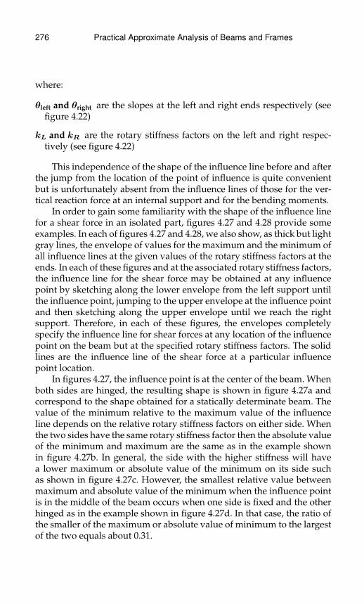
276 Practical Approximate Analysis of Beams and Frames
where:
θleft and θright are the slopes at the left and right ends respectively (seefigure 4.22)
kL and kR are the rotary stiffness factors on the left and right respec-tively (see figure 4.22)
This independence of the shape of the influence line before and afterthe jump from the location of the point of influence is quite convenientbut is unfortunately absent from the influence lines of those for the ver-tical reaction force at an internal support and for the bending moments.
In order to gain some familiarity with the shape of the influence linefor a shear force in an isolated part, figures 4.27 and 4.28 provide someexamples. In each of figures 4.27 and 4.28, we also show, as thick but lightgray lines, the envelope of values for the maximum and the minimum ofall influence lines at the given values of the rotary stiffness factors at theends. In each of these figures and at the associated rotary stiffness factors,the influence line for the shear force may be obtained at any influencepoint by sketching along the lower envelope from the left support untilthe influence point, jumping to the upper envelope at the influence pointand then sketching along the upper envelope until we reach the rightsupport. Therefore, in each of these figures, the envelopes completelyspecify the influence line for shear forces at any location of the influencepoint on the beam but at the specified rotary stiffness factors. The solidlines are the influence line of the shear force at a particular influencepoint location.
In figures 4.27, the influence point is at the center of the beam. Whenboth sides are hinged, the resulting shape is shown in figure 4.27a andcorrespond to the shape obtained for a statically determinate beam. Thevalue of the minimum relative to the maximum value of the influenceline depends on the relative rotary stiffness factors on either side. Whenthe two sides have the same rotary stiffness factor then the absolute valueof the minimum and maximum are the same as in the example shownin figure 4.27b. In general, the side with the higher stiffness will havea lower maximum or absolute value of the minimum on its side suchas shown in figure 4.27c. However, the smallest relative value betweenmaximum and absolute value of the minimum when the influence pointis in the middle of the beam occurs when one side is fixed and the otherhinged as in the example shown in figure 4.27d. In that case, the ratio ofthe smaller of the maximum or absolute value of minimum to the largestof the two equals about 0.31.
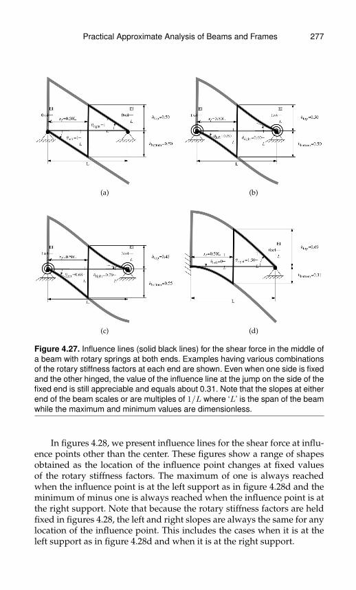
Practical Approximate Analysis of Beams and Frames 277
(a) (b)
(c) (d)
Figure 4.27. Influence lines (solid black lines) for the shear force in the middle ofa beam with rotary springs at both ends. Examples having various combinationsof the rotary stiffness factors at each end are shown. Even when one side is fixedand the other hinged, the value of the influence line at the jump on the side of thefixed end is still appreciable and equals about 0.31. Note that the slopes at eitherend of the beam scales or are multiples of 1/L where ‘L’ is the span of the beamwhile the maximum and minimum values are dimensionless.
In figures 4.28, we present influence lines for the shear force at influ-ence points other than the center. These figures show a range of shapesobtained as the location of the influence point changes at fixed valuesof the rotary stiffness factors. The maximum of one is always reachedwhen the influence point is at the left support as in figure 4.28d and theminimum of minus one is always reached when the influence point is atthe right support. Note that because the rotary stiffness factors are heldfixed in figures 4.28, the left and right slopes are always the same for anylocation of the influence point. This includes the cases when it is at theleft support as in figure 4.28d and when it is at the right support.
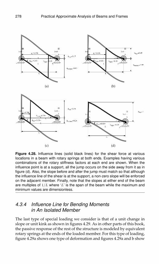
278 Practical Approximate Analysis of Beams and Frames
(a) (b)
(c) (d)
Figure 4.28. Influence lines (solid black lines) for the shear force at variouslocations in a beam with rotary springs at both ends. Examples having variouscombinations of the rotary stiffness factors at each end are shown. When theinfluence point is at a support, all the jump occurs on the side away from it as infigure (d). Also, the slope before and after the jump must match so that althoughthe influence line of the shear is at the support, a non-zero slope will be enforcedon the adjacent member. Finally, note that the slopes at either end of the beamare multiples of 1/L where ‘L’ is the span of the beam while the maximum andminimum values are dimensionless.
4.3.4 Influence Line for Bending Momentsin An Isolated Member
The last type of special loading we consider is that of a unit change inslope or unit kink as shown in figures 4.29. As in other parts of this book,the passive response of the rest of the structure is modeled by equivalentrotary springs at the ends of the loaded member. For this type of loading,figure 4.29a shows one type of deformation and figures 4.29a and b show
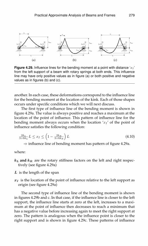
Practical Approximate Analysis of Beams and Frames 279
ΘleftΘright
hmax
kL´4
EI
L
kR´4
EI
L
L
xI
(a)
Θleft
Θright
hmax
hmin
kL´4
EI
L
kR´4
EI
L
L
xI
(b)
Θleft
Θright
hmax
hmin
kL´4
EI
L
kR´4
EI
L
L
xI
(c)
Figure 4.29. Influence lines for the bending moment at a point with distance ‘xI ’from the left support of a beam with rotary springs at both ends. This influenceline may have only positive values as in figure (a) or both positive and negativevalues as in figures (b) and (c).
another. In each case, these deformations correspond to the influence linefor the bending moment at the location of the kink. Each of those shapesoccurs under specific conditions which we will next discuss.
The first type of influence line of the bending moment is shown infigure 4.29a. The value is always positive and reaches a maximum at thelocation of the point of influence. This pattern of influence line for thebending moment always occurs when the location ‘xI ’ of the point ofinfluence satisfies the following condition:
2kL3+6kL
L ≤ xI ≤(
1− 2kR3+6kR
)L (4.10)
⇒ influence line of bending moment has pattern of figure 4.29a.
where:
kL and kR are the rotary stiffness factors on the left and right respec-tively (see figure 4.29a)
L is the length of the span
xI is the location of the point of influence relative to the left support asorigin (see figure 4.29a)
The second type of influence line of the bending moment is shownin figures 4.29b and c. In that case, if the influence line is closer to the leftsupport, the influence line starts at zero at the left, increases to a maxi-mum at the point of influence then decreases to reach a minimum thathas a negative value before increasing again to meet the right support atzero. The pattern is analogous when the influence point is closer to theright support and is shown in figure 4.29c. These patterns of influence

280 Practical Approximate Analysis of Beams and Frames
lines for the bending moment always occurs when the location ‘xI ’ ofthe point of influence satisfies either of the following conditions:
xI ≤ 2kL3+6kL
L (4.11a)
⇒ influence line of bending moment has pattern of figure 4.29b
xI ≥(
1− 2kR3+6kR
)L (4.11b)
⇒ influence line of bending moment has pattern of figure 4.29c
For the purposes of approximating the influence line, we need to identifythe minimum and maximum values (ie. hbottom and htop in figure 4.22),the location of the minimum value and we also need to know the endslopes. The end slopes are needed in order to construct the influencelines of the attached members. We start with the maximum with the exactresult being given by:
hmax = xI
L
(1− xI
L
)×(
(3 + 4kR) + (6kL − 2kR + 8kLkR) (xI/L) (4.12)
− 2 (kL + kR + 4kLkR) (xI/L)2)Lz
where:
z = 3 + 4kL + 4kR + 4kLkR
hmax is the maximum value of the influence line and occurs at the influ-ence point (see any of figures 4.29)
xI is the distance of the point of influence from the left support
L is the length of the beam
kL and kR are the rotary stiffness factors on the left and right respec-tively (see any of figures 4.29)
Formula 4.12 is somewhat complicated but a significantly simpleryet sufficiently accurate approximate expression is currently unavail-able. Of course, the formula reduces correctly to the solution for the max-imum bending moment in a simply supported beam as a unit point forcelocation varies from left to right. In fact, we can obtain simple upper andlower bounds on the maximum influence line value that correspond tothe cases when the beam is simply supported and fixed-fixed respec-tively. The result is then:
2(xI
L
)2 (1− xI
L
)2L ≤ hmax ≤ xI
L
(1− xI
L
)L (4.13)
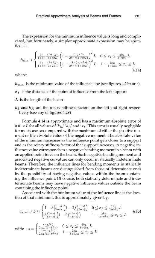
Practical Approximate Analysis of Beams and Frames 281
The expression for the minimum influence value is long and compli-cated, but fortunately, a simpler approximate expression may be speci-fied as:
hmin ≈
kL
1+kL
(1+kR)(5+7kR)
(1− (xI/L)
2kL/(3+6kL)
)2
L 0 ≤ xI ≤ 2kL3+6kL
L
kR1+kR
(1+kL)(5+7kL)
(1− (1−(xI/L))
2kR/(3+6kR)
)2
L 1− 2kR3+6kR
≤ xI ≤ L(4.14)
where:
hmin is the minimum value of the influence line (see figures 4.29b or c)
xI is the distance of the point of influence from the left support
L is the length of the beam
kL and kR are the rotary stiffness factors on the left and right respec-tively (see any of figures 4.29)
Formula 4.14 is approximate and has a maximum absolute error of0.01×L for all values of ‘kL,’ ‘kR’ and ‘xI .’ This error is usually negligiblefor most cases as compared with the maximum of either the positive mo-ment or the absolute value of the negative moment. The absolute valueof the minimum increases as the influence point gets closer to a supportand as the rotary stiffness factor of that support increases. A negative in-fluence value corresponds to a negative bending moment in a beam withan applied point force on the beam. Such negative bending moment andassociated negative curvature can only occur in statically indeterminatebeams. Therefore, the influence lines for bending moments in staticallyindeterminate beams are distinguished from those of determinate onesby the possibility of having negative values within the beam contain-ing the influence point. Of course, both statically determinate and inde-terminate beams may have negative influence values outside the beamcontaining the influence point.
Associated with the minimum value of the influence line is the loca-tion of that minimum, this is approximately given by:
xat min/L ≈
1− 3 (1−s)(3−s)
(1− 2f (1−s)
(2−s)
)0 ≤ xI ≤ 2kL
3+6kLL
3 (1−s)(3−s)
(1− 2f (1−s)
(2−s)
)1− 2kR
3+6kR≤ xI ≤ L
(4.15)
with: s =
{(xI/L)
2kL/(3+6kL) 0 ≤ xI ≤ 2kL3+6kL
L1−(xI/L)
2kR/(3+6kR) 1− 2kR3+6kR
≤ xI ≤ L

282 Practical Approximate Analysis of Beams and Frames
f =
{0.42+0.33kR
1+kR0 ≤ xI ≤ 2kL
3+6kLL
0.42+0.33kL1+kL
1− 2kR3+6kR
≤ xI ≤ Lwhere:
xat min is the location of the minimum value of the influence line fromthe left support
xI is the distance of the point of influence from the left support
L is the length of the beam
kL and kR are the rotary stiffness factors on the left and right respec-tively (see any of figures 4.29)
Note that formula 4.15 has absolute error less than 0.1×L. Althoughthis error is appreciable, it is sufficient for the purpose of approximatelyand manually sketching the shape of the influence lines.
The last result we need in order to approximately but quantitativelyanalyze influence lines for bending moments are expressions for theslopes at the ends of the isolated part. These are exactly given by:
θleft =(3 + 4kR)− (3 + 6kR) (xI/L)
3 + 4kL + 4kR + 4kLkR(4.16a)
θright =(3 + 4kL)− (3 + 6kL) (1− xI/L)
3 + 4kL + 4kR + 4kLkR(4.16b)
where:
xI is the distance of the point of influence from the left support
L is the length of the beam
θleft and θright are the slopes at the left and right ends respectively (seefigure 4.22)
kL and kR are the rotary stiffness factors on the left and right respec-tively (see figure 4.22)
Note that formulas 4.16 allows either slope to be both negative andpositive. If we start with a beam having non-zero rotary stiffness factorsat both ends and with the influence point in the middle of the beam then,if we consider another influence point sufficiently close to one of the sup-ports, negative values in the influence line will appear and the slope atthe support farthest from the influence point will switch sign.
In order to gain some familiarity with the shape of the influence linefor a bending moment in an isolated part, figures 4.30 and 4.31 provide
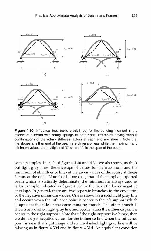
Practical Approximate Analysis of Beams and Frames 283
Θleft=0.50 Θright=0.50
hmax=0.25L
0´4
EI
L
0´4
EI
L
L
xI=0.50L
(a)
Θleft=0.17 Θright=0.17
hmax=0.17L
1´4
EI
L
1´4
EI
L
L
xI=0.50L
(b)
Θleft=0.15 Θright=0.08
hmax=0.15L
1´4
EI
L
3´4
EI
L
L
xI=0.50L
(c)
Θleft=0
Θright=0.25
hmax=0.16L0´4
EI
L
L
xI=0.50L
(d)
Figure 4.30. Influence lines (solid black lines) for the bending moment in themiddle of a beam with rotary springs at both ends. Examples having variouscombinations of the rotary stiffness factors at each end are shown. Note thatthe slopes at either end of the beam are dimensionless while the maximum andminimum values are multiples of ‘L’ where ‘L’ is the span of the beam.
some examples. In each of figures 4.30 and 4.31, we also show, as thickbut light gray lines, the envelope of values for the maximum and theminimum of all influence lines at the given values of the rotary stiffnessfactors at the ends. Note that in one case, that of the simply supportedbeam which is statically determinate, the minimum is always zero asis for example indicated in figure 4.30a by the lack of a lower negativeenvelope. In general, there are two separate branches to the envelopesof the negative minimum values. One is shown as a solid light gray lineand occurs when the influence point is nearer to the left support whichis opposite the side of the corresponding branch. The other branch isshown as a dashed light gray line and occurs when the influence point isnearer to the right support. Note that if the right support is a hinge, thenwe do not get negative values for the influence line when the influencepoint is near that right hinge and so the dashed light gray line will bemissing as in figure 4.30d and in figure 4.31d. An equivalent condition

284 Practical Approximate Analysis of Beams and Frames
Θleft=0.04
Θright=0.38hmax=0.07L
hmin=-0.01L
1´4
EI
L
1´4
EI
L
L
xI=0.85L
(a)
Θleft=0.09Θright=0.18 hmax=0.05L
hmin=-0.04L
1´4
EI
L
3´4
EI
L
L
xI=0.85L
(b)
Θleft=0.33Θright=0
hmax=0.10L1´4
EI
L
3´4
EI
L
L
xI=0.22L
(c)
Θleft=0
Θright=0.50
hmin=-0.19L
0´4
EI
L
L
(d)
Figure 4.31. Influence lines (solid black lines) for the bending moment at variouslocations of a beam with rotary springs at both ends. Examples having variouscombinations of the rotary stiffness factors at each end are shown. Note thatthe slopes at either end of the beam are dimensionless while the maximum andminimum values are multiples of ‘L’ where ‘L’ is the span of the beam.
occurs when the left support is a hinge in which case the lower solidgray line will be missing indicating an absence of a negative minimumenvelope when the influence point is near the left support.
Concerning the upper envelope, the influence line must always passthrough one of those points since there are always positive values ofthe influence line. Furthermore, the maximum always occurs at the kinkwhich is the location of the influence point. The interpretation is thatfor any beam with passive supports and loaded by a unit point force,the maximum bending moment always occurs at the location of the unitpoint force. Note that unlike the influence line for shear forces, the up-per and lower envelopes generally match the influence line at only one(ie. the maximum) or two points (ie. maximum and minimum) ratherthan along whole segments. Finally, in all the figures for the influence
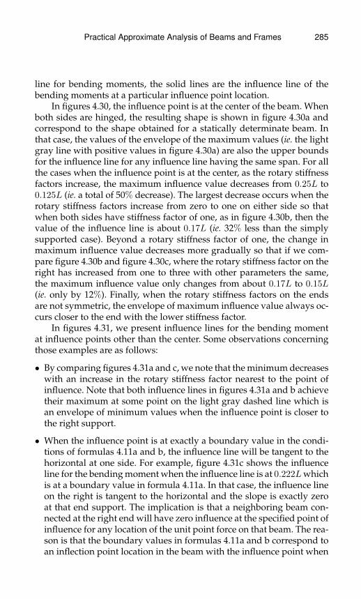
Practical Approximate Analysis of Beams and Frames 285
line for bending moments, the solid lines are the influence line of thebending moments at a particular influence point location.
In figures 4.30, the influence point is at the center of the beam. Whenboth sides are hinged, the resulting shape is shown in figure 4.30a andcorrespond to the shape obtained for a statically determinate beam. Inthat case, the values of the envelope of the maximum values (ie. the lightgray line with positive values in figure 4.30a) are also the upper boundsfor the influence line for any influence line having the same span. For allthe cases when the influence point is at the center, as the rotary stiffnessfactors increase, the maximum influence value decreases from 0.25L to0.125L (ie. a total of 50% decrease). The largest decrease occurs when therotary stiffness factors increase from zero to one on either side so thatwhen both sides have stiffness factor of one, as in figure 4.30b, then thevalue of the influence line is about 0.17L (ie. 32% less than the simplysupported case). Beyond a rotary stiffness factor of one, the change inmaximum influence value decreases more gradually so that if we com-pare figure 4.30b and figure 4.30c, where the rotary stiffness factor on theright has increased from one to three with other parameters the same,the maximum influence value only changes from about 0.17L to 0.15L(ie. only by 12%). Finally, when the rotary stiffness factors on the endsare not symmetric, the envelope of maximum influence value always oc-curs closer to the end with the lower stiffness factor.
In figures 4.31, we present influence lines for the bending momentat influence points other than the center. Some observations concerningthose examples are as follows:
• By comparing figures 4.31a and c, we note that the minimum decreaseswith an increase in the rotary stiffness factor nearest to the point ofinfluence. Note that both influence lines in figures 4.31a and b achievetheir maximum at some point on the light gray dashed line which isan envelope of minimum values when the influence point is closer tothe right support.
• When the influence point is at exactly a boundary value in the condi-tions of formulas 4.11a and b, the influence line will be tangent to thehorizontal at one side. For example, figure 4.31c shows the influenceline for the bending moment when the influence line is at 0.222Lwhichis at a boundary value in formula 4.11a. In that case, the influence lineon the right is tangent to the horizontal and the slope is exactly zeroat that end support. The implication is that a neighboring beam con-nected at the right end will have zero influence at the specified point ofinfluence for any location of the unit point force on that beam. The rea-son is that the boundary values in formulas 4.11a and b correspond toan inflection point location in the beam with the influence point when

286 Practical Approximate Analysis of Beams and Frames
any load is applied to another beam attached on the right or on the leftof it respectively.
• Finally, if we consider an influence point that is at exactly the left orat exactly the right support, then the influence values will all be nega-tive as shown in example 4.31d where the influence point is exactly atthe left support. In those cases, the minimum influence value will bethe minimum value of either the left or the right lower envelope de-pending on whether the influence point is at the right or left supportrespectively. Also note that the slope at the end that is obtained by for-mula 4.16a and b when an influence point is right at a support is theslope of the neighboring member attached to that end rather than theslope of the influence line itself. For example, in figure 4.31d, the slopeat the left support is identified to be zero based on formula 4.16a whichis the slope of the fixed end rather than the slope of the influence lineat that end.
4.3.5 Influence Line in a Transition Member for All Types
In the approach we present to obtain influence lines, we start by isolat-ing the beam containing the influence point. When isolating that beam,we model the rest of the structure attached to either end by equivalentrotary springs. Once isolated, we sketch that beam’s influence line basedon the results presented in the previous sections. In addition, we obtainthe slopes at either end of that isolated beam. Those slopes are then ap-plied at the ends of the beams attached to that isolated beam which inturn may be attached to other beams. Therefore, each of the beams otherthan the one containing the influence point has basically the same config-uration if it has no internal hinges. Those beams are unloaded but have aspecified slope on one side and a passive structure attached to the other.This implies that they may be modeled as shown in figure 4.32 with anapplied slope at one end which we call the near end and a rotary springat the other end whcih we call the far end. Based on the Muller-Breslauprinciple if we determine the deformation of such a beam then this de-formation corresponds to their influence line.
The beam shown in figure 4.32 is fundamental in this book and hasbeen analyzed and used several times in previous chapters. The currentfocus is to obtain the following pieces of information:
• The maximum displacement ‘umax’ in terms of the applied slope ‘θnear’(see figure 4.32). Note that in previous studies, we applied a momentrather that a slope.

Practical Approximate Analysis of Beams and Frames 287
Θnear
Θfar
umax
xat max
k´4
EI
L
L
Figure 4.32. Transition member used to sketch influence lines of the membersnot containing the influence point.
• The approximate location ‘xat max’ of the maximum displacement. Thishas been extensively done in a previous chapter
• The slope at the far end ‘θfar’ in terms of the applied or near end slope‘θnear.’
First, we consider the slope at the far end which is exactly given by:
θfar/θnear =1
2 + 2k(4.17)
where:
θnear and θfar are the slopes at the ends of the beam where ‘θnear’ is con-sidered as an applied slope (see figure 4.32)
k is the rotary stiffness factor at the far end (see figure 4.32)
Note that the ratio in equation 4.16 is a uniformly decreasing func-tion of ‘k’ with the fastest decrease occuring between zero and one.
The next result is the maximum displacement ‘umax’ and this is ap-proximately given by:
umax ≈ 0.19+0.15k1+k θnearL (4.18)
where:
θnear is the applied slope at one end of the beam (see figure 4.32)
k is the rotary stiffness factor at the far end (see figure 4.32)
L is the span or length of the beam (see figure 4.32)
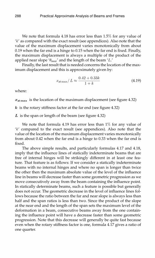
288 Practical Approximate Analysis of Beams and Frames
We note that formula 4.18 has error less than 1.5% for any value of‘k’ as compared with the exact result (see appendices). Also note that thevalue of the maximum displacement varies monotonically from about0.19 when the far end is a hinge to 0.15 when the far end is fixed. Finally,the maximum displacement is always a multiple of the product of theapplied near slope ‘θnear’ and the length of the beam ‘L.’
Finally, the last result that is needed concerns the location of the max-imum displacement and this is approximately given by:
xat max/L ≈ 0.42 + 0.33k
1 + k(4.19)
where:
xat max is the location of the maximum displacement (see figure 4.32)
k is the rotary stiffness factor at the far end (see figure 4.32)
L is the span or length of the beam (see figure 4.32)
We note that formula 4.19 has error less than 1% for any value of‘k’ compared to the exact result (see appendices). Also note that thevalue of the location of the maximum displacement varies monotonicallyfrom about 0.42 when the far end is a hinge to 0.33 when the far end isfixed.
The above simple results, and particularly formulas 4.17 and 4.18,imply that the influence lines of statically indeterminate beams that arefree of internal hinges will be strikingly different in at least one fea-ture. That feature is as follows: If we consider a statically indeterminatebeams with no internal hinges and where no span is longer than twicethe other then the maximum absolute value of the level of the influenceline in beams will decrease faster than some geometric progression as wemove consecutively away from the beam containing the influence point.In statically determinate beams, such a feature is possible but generallydoes not occur. The geometric decrease in the level of influence lines fol-lows because the ratio between the far and near slope is always less thanhalf and the span ratios is less than two. Since the product of the slopeat the near end and the length of the span sets the maximum level of thedeformation in a beam, consecutive beams away from the one contain-ing the influence point will have a decrease faster than some geometricprogression. Note that this decrease will generally be quite fast becauseeven when the rotary stiffness factor is one, formula 4.17 gives a ratio ofone quarter.

Practical Approximate Analysis of Beams and Frames 289
4.3.6 Examples of Sketching Influence Linesfor Vertical Force Reactions
In this section, we will present examples of sketching the influence linesfor vertical force reactions. The results in the figures shown are exactresults and we will describe how the discussions and approximationsdeveloped in previous sections allow us to approximately sketch thoseinfluence lines. For simplicity, we will start with examples where all thespans are equal and have the same sectional properties as shown in fig-ure 4.33. As specific examples, we will consider the influence line for thevertical reaction at A and for the vertical reaction at C. The rest of thecases shown in figure 4.33 may be similarly analyzed and are left as anexercise for the reader.
beam
1
EI=1
1
EI=1
1
EI=1
1
EI=1
A B C D E
Vertical reaction at A
0. 0.5 1. 1.5 2. 2.5 3. 3.5 4.-0.25
0.
0.25
0.5
0.75
1.
span xat min hmin xat max hmax
1 1 0 0 1
2 0.380 −0.079 1 0
3 0 0 0.377 0.021
4 0.333 −0.005 1 0
Figure 4.33. Influence lines for the vertical force reactions in a case whereall beams have the same span and the same sectional properties. (Continuedbelow.)

290 Practical Approximate Analysis of Beams and Frames
Vertical reaction at B
0. 0.5 1. 1.5 2. 2.5 3. 3.5 4.-0.25
0.
0.25
0.5
0.75
1.
span xat min hmin xat max hmax
1 0 0 0.939 1.007
2 1 0 0 1
3 0.377 −0.125 1 0
4 0 0 0.333 0.027
Vertical reaction at C
0. 0.5 1. 1.5 2. 2.5 3. 3.5 4.-0.25
0.
0.25
0.5
0.75
1.
span xat min hmin xat max hmax
1 0.577 −0.167 1 0
2 0 0 0.993 1.000
3 1 0 0 1
4 0.333 −0.110 1 0
Figure 4.33. (Continued from above and continued below.)

Practical Approximate Analysis of Beams and Frames 291
Vertical reaction at D
0. 0.5 1. 1.5 2. 2.5 3. 3.5 4.-0.25
0.
0.25
0.5
0.75
1.
span xat min hmin xat max hmax
1 0 0 0.577 0.048
2 0.616 −0.149 1 0
3 0 0 0.956 1.005
4 1 0 0 1
Vertical reaction at E
0. 0.5 1. 1.5 2. 2.5 3. 3.5 4.-0.25
0.
0.25
0.5
0.75
1.
span xat min hmin xat max hmax
1 0.577 −0.012 1 0
2 0 0 0.616 0.037
3 0.619 −0.137 1 0
4 0 0 1 1
Figure 4.33. (Continued from above.) Influence lines for the vertical force reac-tions in a case where all beams have the same span and the same sectionalproperties.
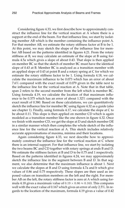
292 Practical Approximate Analysis of Beams and Frames
Considering figure 4.33, we first describe how to approximately con-struct the influence line for the vertical reaction at A where there is asupport at the end of the beam. For that influence line, we start by isolat-ing member AB which is the member containing the influence point A.For that member AB, we estimate the rotary stiffness factor at B to be 1.At this point, we may sketch the shape of the influence line for mem-ber AB based on the patterns identified in figures 4.21. From the rotarystiffness at B, we may calculate an estimate of the slope at B using for-mula 4.5a which gives a slope of about 0.43. That slope is then appliedon member BC so that the sketch of member BC must have the identicalslope of 0.43 at B. Member BC is analyzed as a transition member withan applied slope of 0.43 at point B and a rotary spring at C for which weestimate the rotary stiffness factor to be 1. Using formula 4.18, we cal-culate the maximum influence to be 0.073 which has an error of about7.6% compared with the exact result of 0.079 given in the table next tothe influence line for the vertical reaction at A. Note that in that table,span 2 refers to the second member from the left which is member BC.Using formula 4.19, we calculate the location of that maximum influ-ence to be 0.375 which has an error of about 1.32% compared with theexact result of 0.380. Based on these calculations, we can quantitativelysketch the influence line for member BC using figure 4.32 as a guide (alsosee chapter 1). Finally, using formula 4.17, we calculate the slope at C tobe about 0.11. This slope is then applied on member CD which is againmodeled as a transition member like the one shown in figure 4.32. Oncewe finish with member CD, we get the slope at D and sketch member DEin a similar manner which then completes the whole sketch of the influ-ence line for the vertical reaction at A. This sketch includes relativelyaccurate approximations of maxima, minima and their locations.
Again considering figure 4.33, we next describe how to approxi-mately construct the influence line for the vertical reaction at C wherethere is an internal support. For that influence line, we start by isolatingthe two beams BC and CD together with rotary springs at ends B and D.We estimate the stiffness factors at B and D to be 0.75 and 1 respectively.Based on the patterns identified in figures 4.24, we may approximatelysketch the influence line in the segment between B and D. In that seg-ment, we also determine that the maximum influence is about 1. Nextwe calculate the slopes at B and D using formula 4.7a and b which givevalues of 0.86 and 0.75 respectively. These slopes are then used as im-posed values on transition members on the left and the right. For mem-ber AB on the left, the rotary stiffness factor is zero at A which using for-mula 4.18 gives a maximum value of 0.19× 0.86 ≈ 0.163. This compareswell with the exact value of 0.167 which gives an error of only 2.5%. In re-gards to the location of the maximum, formula 4.19 gives a value of 0.42

Practical Approximate Analysis of Beams and Frames 293
from the location of the imposed slope which is point B or equivalently1 − 0.42 = 0.57 from point A. This value again compares well with theexact value of 0.577 corresponding to an error of only 1.21%. For mem-ber CD on the right of the isolated segment BCD, the rotary stiffness fac-tor is infinity at D due to the fixed end. Applying a slope at D of 0.75 andusing formulas 4.18 and 4.19, we get values of 0.15 × 0.75 ≈ 0.112 and0.33 for the maximum influence and location respectively. These againcompare well with the exact values of 0.110 and 0.333 given for span 4 inthe table next to the exact influence line.
Next we consider the beam shown in figure 4.34 where the spans arenonequal and the sectional properties are different. As specific examples,we will consider the influence line for the vertical reaction at E and forthe vertical reaction at B. The rest of the cases may be similarly analyzedand are left as an exercise for the reader.
Considering figure 4.34, we first describe how to approximately con-struct the influence line for the vertical reaction at E where there is asupport at the end of the beam. For that influence line, we start by isolat-ing member DE which is the member containing the influence point E.For that member DE, we estimate the rotary stiffness factor at D to be(1/1.5)/(0.8/0.75) ≈ 0.625. At this point, we may sketch the shape ofthe influence line for member DE based on the patterns identified in fig-ures 4.22. From the rotary stiffness factor at D, we may calculate an es-timate of the slope at using formula 4.5b which gives a slope of about1.231. That slope is then applied on member DC so that the sketch ofmember DC must have the identical slope of 1.231 at D. Member DCis analyzed as a transition member with an applied slope of 1.231 atpoint D and a rotary spring at C for which we estimate the rotary stiff-ness factor to be (0.8/0.75)/(1/1.5) ≈ 1.6. Using formula 4.18, we cal-culate the maximum influence to be 0.305 which has an error of about4.1% compared with the exact result of 0.318 given in the table next tothe influence line for the vertical reaction at D. Note that in that table,span 3 refers to the third member from the left which is member CD.Using formula 4.19, we calculate the location of that maximum influ-ence to be 0.547 from the left support or 1.5 − 0.547 ≈ 0.953 from theleft support C which has an error of about 0.95% compared with theexact result of 0.944. Based on these calculations, we can quantitativelysketch the influence line for member CD using figure 4.32 as a guide(also see chapter 1). Finally, using formula 4.17, we calculate the slopeat C to be about 0.237. This slope is then applied on member CB which isagain modeled as a transition member like the one shown in figure 4.32.Once we finish with member CB, we get the slope at D and sketchmember AB in a similar manner which then completes the whole sketchof the influence line for the vertical reaction at E. This sketch includes
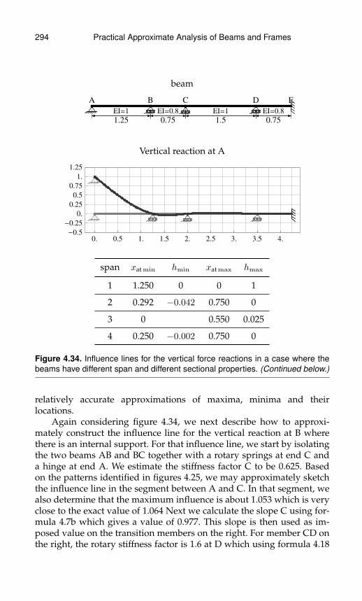
294 Practical Approximate Analysis of Beams and Frames
beam
1.25
EI=1
0.75
EI=0.8
1.5
EI=1
0.75
EI=0.8
A B C D E
Vertical reaction at A
0. 0.5 1. 1.5 2. 2.5 3. 3.5 4.-0.5
-0.25
0.
0.25
0.5
0.75
1.
1.25
span xat min hmin xat max hmax
1 1.250 0 0 1
2 0.292 −0.042 0.750 0
3 0 0.550 0.025
4 0.250 −0.002 0.750 0
Figure 4.34. Influence lines for the vertical force reactions in a case where thebeams have different span and different sectional properties. (Continued below.)
relatively accurate approximations of maxima, minima and theirlocations.
Again considering figure 4.34, we next describe how to approxi-mately construct the influence line for the vertical reaction at B wherethere is an internal support. For that influence line, we start by isolatingthe two beams AB and BC together with a rotary springs at end C anda hinge at end A. We estimate the stiffness factor C to be 0.625. Basedon the patterns identified in figures 4.25, we may approximately sketchthe influence line in the segment between A and C. In that segment, wealso determine that the maximum influence is about 1.053 which is veryclose to the exact value of 1.064 Next we calculate the slope C using for-mula 4.7b which gives a value of 0.977. This slope is then used as im-posed value on the transition members on the right. For member CD onthe right, the rotary stiffness factor is 1.6 at D which using formula 4.18
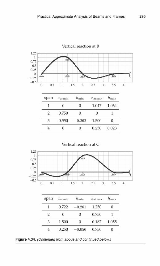
Practical Approximate Analysis of Beams and Frames 295
Vertical reaction at B
0. 0.5 1. 1.5 2. 2.5 3. 3.5 4.-0.5
-0.25
0.
0.25
0.5
0.75
1.
1.25
span xat min hmin xat max hmax
1 0 0 1.047 1.064
2 0.750 0 0 1
3 0.550 −0.262 1.500 0
4 0 0 0.250 0.023
Vertical reaction at C
0. 0.5 1. 1.5 2. 2.5 3. 3.5 4.-0.5
-0.25
0.
0.25
0.5
0.75
1.
1.25
span xat min hmin xat max hmax
1 0.722 −0.261 1.250 0
2 0 0 0.750 1
3 1.500 0 0.187 1.055
4 0.250 −0.056 0.750 0
Figure 4.34. (Continued from above and continued below.)

296 Practical Approximate Analysis of Beams and Frames
Vertical reaction at D
0. 0.5 1. 1.5 2. 2.5 3. 3.5 4.-0.5
-0.25
0.
0.25
0.5
0.75
1.
1.25
span xat min hmin xat max hmax
1 0 0 0.722 0.049
2 0.458 −0.083 0.750 0
3 0 0 1.248 1.116
4 0.750 0 0 1
Vertical reaction at E
0. 0.5 1. 1.5 2. 2.5 3. 3.5 4.-0.5
-0.25
0.
0.25
0.5
0.75
1.
1.25
span xat min hmin xat max hmax
1 0.722 −0.021 1.250 0
2 0 0 0.458 0.036
3 0.944 −0.318 1.500 0
4 0 0 0.750 1
Figure 4.34. (Continued from above.) Influence lines for the vertical force re-actions in a case where the beams have different span and different sectionalproperties.
Practical Approximate Analysis of Beams and Frames 297
gives a maximum value of 0.977 ∗ 1.5(0.19 + 0.15 ∗ 1.6)/(1 + 1.6) ≈ 0.242.This compares well with the exact value of 0.262 which gives an errorof 7.6%. In regards to the location of the maximum, formula 4.19 gives avalue of 0.547 from the location of the imposed slope which is point C.This value again compares well with the exact value of 0.550 correspond-ing to an error of 0.55%. Next we use formula 4.17 to get the slope at Dwhich gives a value of 0.188. This slope is then applied at D on mem-ber DE to sketch that member and to complete the influence line. Thissketch of the influence line includes relatively accurate approximationsof maxima, minima and their locations.
4.3.7 Examples of Sketching Influence Linesfor Shear Forces
In this section, we will present examples of sketching the influence linesfor shear forces. The results in the figures shown are exact results andwe will describe how the discussions and approximations developed inprevious sections allow us to approximately sketch those influence lines.For simplicity, we will start with examples where all the spans are equaland have the same sectional properties as shown in figure 4.35. As a spe-cific example, we will consider the influence lines for the shear force atpoint D. The rest of the cases shown in figure 4.35 may be similarly ana-lyzed and are left as an exercise for the reader.
Considering figure 4.35, we describe how to approximately constructthe influence line for the shear force at D. For that influence line, we startby isolating member CE which is the member containing the influencepoint D. For that member CE, we estimate the rotary stiffness factors at Cand E to be 0.75 and 1 respectively. Next, using formula 4.8a and b wecalculate the values before and after the influence point D to be 0.514and 0.486 respectively. These values have an error of 1.18% and 1.22% re-spectively compared with the exact result shown in a table near the cor-responding figure for the influence line at span 2 which is member CE(ie. second span from the left). With these values and figures 4.27 and 4.28as a guide, we can sketch the influence line for member CE. To proceedfurther, we calculate the slopes at C and E using formula 4.9a and bwhich give the values of 0.692 and 0.577 respectively. These slopes arethen used as imposed values on transition members on the left and theright. For member AC on the left, the rotary stiffness factor is zero at Awhich using formula 4.18 gives a maximum value of 0.19×0.692 ≈ 0.131which is, to the specified precision, the exact result. The location of thatmaximum is calculated using formula 4.19 which gives a value of 0.42from the location of the imposed slope which is point C or equivalently1 − 0.42 = 0.57 from point A. This value again compares well with the

298 Practical Approximate Analysis of Beams and Frames
beam
1
EI=1
0.3
1
EI=1
0.5
1
EI=1
0.1
1
EI=1
0.4
A B C D E FG H I
Shear force at B
0. 0.5 1. 1.5 2. 2.5 3. 3.5 4.-0.5
-0.25
0.
0.25
0.5
0.75
span xat min hmin xat max hmax
1 0.300 −0.373 0.300 0.627
2 0.380 −0.079 1 0
3 0 0 0.377 0.021
4 0.333 −0.005 1 0
Figure 4.35. Influence lines for the shear forces in a case where all beams havethe same span and the same sectional properties. (Continued below.)
exact value of 0.577 corresponding to an error of only 1.21%. With thisinformation, we can then sketch the influence line for the member AC.Next we consider the member on the right of the isolated member CEwhich is member EG. Again we use the transition member shown in fig-ure 4.32 with an applied slope obtained above as 0.577 at point E andwe estimate the rotary stiffness factor at G to be 1. Using formulas 4.18and 4.19, we obtain the maximum influence value and location to be0.098 and 0.375 respectively which compare well with the exact resultsof 0.104 (ie. 5.8% error) and 0.377 (ie. 0.53% error) respectively. To finishwith member EG, we obtain the slope at G using formula 4.17 whichgives a value of about 0.14. Based on these calculations for member EG,we can quantitatively sketch its influence line using figure 4.32 as a guide(also see chapter 1). The influence line of the last member GI may be sim-ilarly sketched using the imposed slope of 0.14 at point G, figure 4.32 as

Practical Approximate Analysis of Beams and Frames 299
Shear force at D
0. 0.5 1. 1.5 2. 2.5 3. 3.5 4.-0.5
-0.25
0.
0.25
0.5
span xat min hmin xat max hmax
1 0 0 0.577 0.131
2 0.500 −0.508 0.500 0.492
3 0.377 −0.104 1 0
4 0 0 0.333 0.023
Shear force at F
0. 0.5 1. 1.5 2. 2.5 3. 3.5 4.-1.
-0.75
-0.5
-0.25
0.
0.25
span xat min hmin xat max hmax
1 0.577 −0.036 1 0
2 0 0 0.616 0.111
3 0.900 −0.930 0.900 0.070
4 0.333 −0.087 1 0
Figure 4.35. (Continued from above and continued below.)
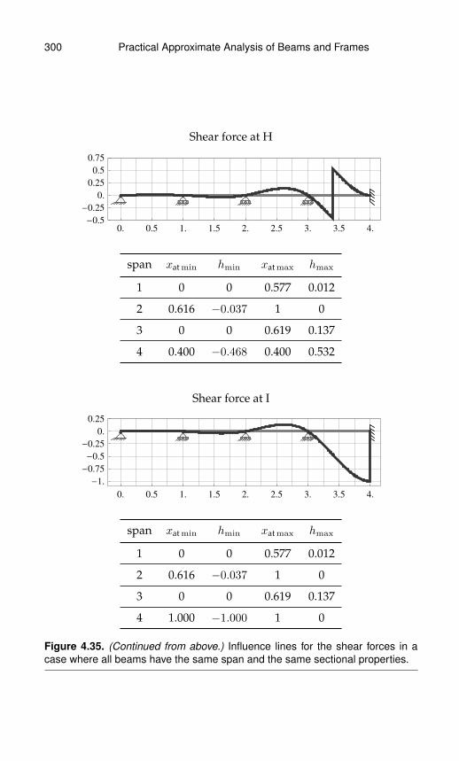
300 Practical Approximate Analysis of Beams and Frames
Shear force at H
0. 0.5 1. 1.5 2. 2.5 3. 3.5 4.-0.5
-0.25
0.
0.25
0.5
0.75
span xat min hmin xat max hmax
1 0 0 0.577 0.012
2 0.616 −0.037 1 0
3 0 0 0.619 0.137
4 0.400 −0.468 0.400 0.532
Shear force at I
0. 0.5 1. 1.5 2. 2.5 3. 3.5 4.
-1.
-0.75
-0.5
-0.25
0.
0.25
span xat min hmin xat max hmax
1 0 0 0.577 0.012
2 0.616 −0.037 1 0
3 0 0 0.619 0.137
4 1.000 −1.000 1 0
Figure 4.35. (Continued from above.) Influence lines for the shear forces in acase where all beams have the same span and the same sectional properties.

Practical Approximate Analysis of Beams and Frames 301
a guide with k → ∞ and with the formulas associated with that figure.This then would complete the whole sketch of the influence line for theshear force at D. This sketch includes relatively accurate approximationsof maxima, minima and their locations.
Next we consider the beam shown in figure 4.36 where the spans arenonequal and the sectional properties are different. As specific examples,we will consider the influence line for the shear forces at B+ and at F. Therest of the cases may be similarly analyzed and are left as an exercise forthe reader.
Considering figure 4.36, we first describe how to approximately con-struct the influence line for the shear force at a point just to the right ofpoint B which we refer to as point B+. For that influence line, we startby isolating member BC which is the member containing the influencepoint B+. For that member BC, we estimate the rotary stiffness factors
beam
1.25
EI=1
0.75
EI=0.8
1.5
EI=1
0.75
0.75
EI=0.8
0.3
A B C D E F G
Shear force at B−
0. 0.5 1. 1.5 2. 2.5 3. 3.5 4.
-1.
-0.75
-0.5
-0.25
0.
span xat min hmin xat max hmax
1 1.250 −1.000 1.250 0
2 0.292 −0.042 0.750 0
3 0 0 0.550 0.025
4 0.250 −0.002 0.750 0
Figure 4.36. Influence lines for the shear forces in a case where the beams havedifferent span and different sectional properties. (Continued below.)

302 Practical Approximate Analysis of Beams and Frames
Shear force at B+
0. 0.5 1. 1.5 2. 2.5 3. 3.5 4.
-0.25
0.
0.25
0.5
0.75
1.
span xat min hmin xat max hmax
1 0 0 0.722 0.233
2 0 0 0.000 1.000
3 0.550 −0.237 1.500 0
4 0 0 0.250 0.021
Shear force at D
0. 0.5 1. 1.5 2. 2.5 3. 3.5 4.
-0.5
-0.25
0.
0.25
0.5
span xat min hmin xat max hmax
1 0.722 −0.028 1.250 0
2 0 0 0.458 0.047
3 0.750 −0.508 0.750 0.492
4 0.250 −0.035 0.750 0
Figure 4.36. (Continued from above and continued below.)

Practical Approximate Analysis of Beams and Frames 303
Shear force at F
0. 0.5 1. 1.5 2. 2.5 3. 3.5 4.
-0.5
-0.25
0.
0.25
0.5
span xat min hmin xat max hmax
1 0 0 0.722 0.021
2 0.458 −0.036 0.750 0
3 0 0 0.944 0.318
4 0.300 −0.490 0.300 0.509
Shear force at G
0. 0.5 1. 1.5 2. 2.5 3. 3.5 4.
-1.
-0.75
-0.5
-0.25
0.
0.25
0.5
span xat min hmin xat max hmax
1 0 0 0.722 0.021
2 0.458 −0.036 0.750 0
3 0 0 0.944 0.318
4 0.750 −1.000 0.750 0
Figure 4.36. (Continued from above.) Influence lines for the shear forces in acase where the beams have different span and different sectional properties.

304 Practical Approximate Analysis of Beams and Frames
at B and C to be 0.563 and 0.625 respectively. Next, either based on kine-matic constraints or using formula 4.8a and b we identify the values be-fore and after the influence point D to be 0 and 1 respectively which arethe same as the exact results. With these values and figures 4.28d as aguide, we can sketch the influence line for member BC. From the esti-mates of the rotary stiffness factors at B and C, we may use formula 4.9ato calculate estimates of the slopes B and C which give 0.983 and 0.928respectively. Those slopes are applied on the neighboring members ABand CD respectively using the transition model of figure 4.32. Startingwith member AB, we have the rotary stiffness factor at the left equalzero because of the hinge at the end. Using formula 4.18 with the ap-plied slope of 0.983 at B, we obtain the maximum influence value as 0.233which is the exact result up to the precision of the calculations. As for thelocation of that maximum value, formula 4.19 gives a value of 0.525 frompoint B which is (1.25 − 0.525) = 0.725 from point A and is very closeto the exact result of 0.722. At this point, we use the calculated values tosketch the influence line for member AB using figure 4.32 as a guide (alsosee chapter 1). Next we consider member CE as a transition member withan applied slope of 0.928 at C and a spring with rotary stiffness factor of1.6 at E. Using formulas 4.18 and 4.19, we get the magnitude and loca-tion of the maximum influence value to be 0.230 and 0.547 respectivelywhich are very close to the exact results of 0.237 (ie. about 2.5% error) and0.550 (ie. about 0.55% error) respectively. With these values, member CEcan be sketched using figure 4.32 as a guide (also see chapter 1). Consid-ering member CE, we can also calculate the slope at E using 4.17 whichgives a slope of 0.178 at point E. This slope is then imposed at point Eof member EG with the model of figure 4.32 in order to calculate valuesand to sketch the influence line for member EG. This then completes thesketch for the whole influence line for the shear force at point B+ and in-cludes relatively accurate approximations of maxima, minima and theirlocations.
Again considering figure 4.36, we next describe how to approxi-mately construct the influence line for the shear force at F. For that in-fluence line, we start by isolating member EG which is the member con-taining the influence point F. For that member EG, we estimate the rotarystiffness factor at the left to be 0.625 while that at the right is infinite dueto the fixed end. Next we use formula 4.8a and b to calculate the val-ues before and after the influence point F which we find to be 0.485 and0.515 respectively. These values compare well with the exact values of0.490 (ie. about 1.02% error) and 0.509 (ie. about 1.18% error) respectively.With these values and figures 4.27 and 4.28 as a guide, we can sketch theinfluence line for member EG. With the same isolated member EG, wemay use formula 4.9a to calculate estimates of the slope at E which gives
Practical Approximate Analysis of Beams and Frames 305
a slope of 1.23. This slope is applied on the neighboring member CE atpoint E using the transition model of figure 4.32 and we estimate of therotary spring factor at point C to be 1.6. Using formulas 4.18 and 4.19,we get the magnitude and location of the maximum influence value tobe 0.305 and 0.547 from the right end (ie. 0.953 from the left end) respec-tively which are very close to the exact results of 0.318 (ie. about 4.1% er-ror) and 0.944 (ie. about 0.95% error) respectively. Based on these calcula-tions, we can quantitatively sketch the influence line for member CE us-ing figure 4.32 as a guide (also see chapter 1). Finally, using formula 4.17,we calculate the slope at C to be about 0.237. This slope is then appliedon member BC which is again modeled as a transition member like theone shown in figure 4.32. Once we finish with member BC, we get theslope at B and sketch member AB in a similar manner which then com-pletes the whole sketch of the influence line for the shear force at F. Thissketch includes relatively accurate approximations of maxima, minimaand their locations.
4.3.8 Examples of Sketching Influence Linesfor Bending Moments
In this section, we will present examples of sketching the influence linesfor bending moments. The results in the figures shown are exact resultsand we will describe how the discussions and approximations devel-oped in previous sections allow us to approximately sketch those influ-ence lines. For simplicity, we will start with examples where all the spansare equal and have the same sectional properties as shown in figure 4.37.As a specific example, we will consider the influence lines for the bend-ing moment at point F. The rest of the cases shown in figure 4.37 may besimilarly analyzed and are left as an exercise for the reader.
Considering figure 4.37, we describe how to approximately constructthe influence line for the shear force at F. For that influence line, we startby isolating member EG which is the member containing the influencepoint F. For that member EG, we estimate the rotary stiffness factors at Eand G to be both equal to one. Next, using formula 4.12, we calculate thevalue of the maximum positive value which always occurs at the point ofinfluence to be 0.048 which, up to the precision used, is the exact result.At this point, we have to determine the shape pattern of the influenceline over that member. We may do that by checking each of formulas 4.10and 4.11a and b where we find that condition 4.11b is true which impliesthat the pattern of deformation is that of figure 4.29c. This also meansthat we need to calculate the value and location of the minimum (ie. low-ermost negative value). We do this using formulas 4.14 and 4.15 whichgive 0.025 and 0.475 respectively. We compare these values with the exact

306 Practical Approximate Analysis of Beams and Frames
beam
1
EI=1
0.3
1
EI=1
0.5
1
EI=1
0.1
1
EI=1
A B C D E FG H
Bending moment at B
0. 0.5 1. 1.5 2. 2.5 3. 3.5 4.-0.05
0.
0.05
0.1
0.15
0.2
span xat min hmin xat max hmax
1 0 0 0.300 0.188
2 0.380 −0.024 1 0
3 0 0 0.377 0.006
4 0.333 −0.001 1 0
Figure 4.37. Influence lines for the bending moments in a case where all beamshave the same span and the same sectional properties. (Continued below.)
results which are 0.035 (ie. about 28.6% error) and 0.467 (ie. about 1.71%error). While the error in the minimum value is appreciable, it is suffi-cient for an approximate analysis and the overall pattern of the influenceline for member EG is still well-represented. At this point, we may sketchthe influence line for member EG using the calculated values and eitherfigure 4.29c or figure 4.31b as a guide. To proceed further, we calculatethe slopes at E and G using formula 4.16a and b which give the valuesof 0.073 and 0.407 respectively. These slopes are then used as imposedvalues on transition members on the left and the right. For member GHon the right, the rotary stiffness factor is infinity at H because of the fixedend. Using formula 4.18 and 4.19 with the imposed slope of 0.407, weget a maximum value and location of 0.061 and 0.33 respectively whichcompare well with the exact results of 0.060 (ie. about 1.67% error) and0.333 (ie. about 0.91% error) respectively. Based on these calculations for
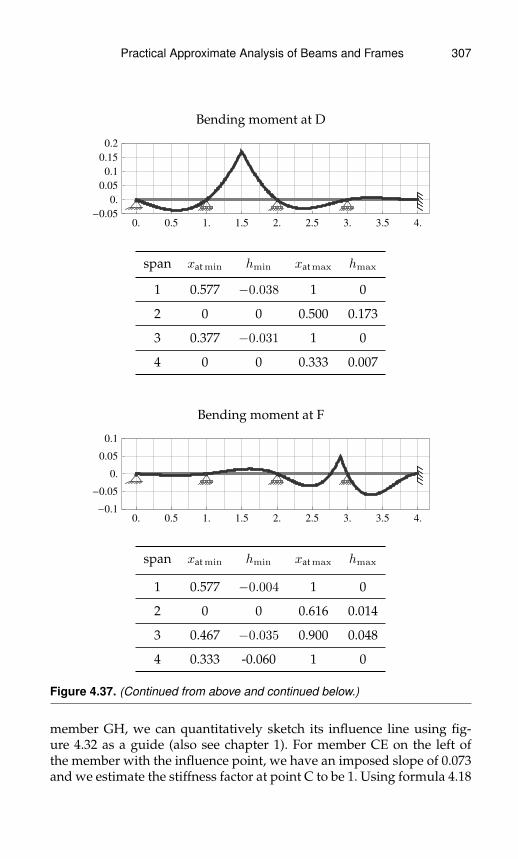
Practical Approximate Analysis of Beams and Frames 307
Bending moment at D
0. 0.5 1. 1.5 2. 2.5 3. 3.5 4.-0.05
0.
0.05
0.1
0.15
0.2
span xat min hmin xat max hmax
1 0.577 −0.038 1 0
2 0 0 0.500 0.173
3 0.377 −0.031 1 0
4 0 0 0.333 0.007
Bending moment at F
0. 0.5 1. 1.5 2. 2.5 3. 3.5 4.-0.1
-0.05
0.
0.05
0.1
span xat min hmin xat max hmax
1 0.577 −0.004 1 0
2 0 0 0.616 0.014
3 0.467 −0.035 0.900 0.048
4 0.333 -0.060 1 0
Figure 4.37. (Continued from above and continued below.)
member GH, we can quantitatively sketch its influence line using fig-ure 4.32 as a guide (also see chapter 1). For member CE on the left ofthe member with the influence point, we have an imposed slope of 0.073and we estimate the stiffness factor at point C to be 1. Using formula 4.18
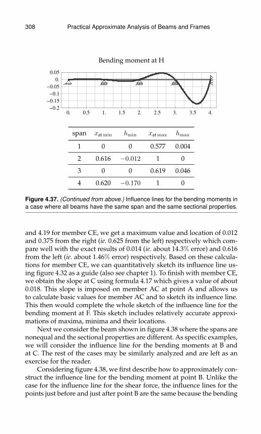
308 Practical Approximate Analysis of Beams and Frames
Bending moment at H
0. 0.5 1. 1.5 2. 2.5 3. 3.5 4.-0.2
-0.15
-0.1
-0.05
0.
0.05
span xat min hmin xat max hmax
1 0 0 0.577 0.004
2 0.616 −0.012 1 0
3 0 0 0.619 0.046
4 0.620 −0.170 1 0
Figure 4.37. (Continued from above.) Influence lines for the bending moments ina case where all beams have the same span and the same sectional properties.
and 4.19 for member CE, we get a maximum value and location of 0.012and 0.375 from the right (ie. 0.625 from the left) respectively which com-pare well with the exact results of 0.014 (ie. about 14.3% error) and 0.616from the left (ie. about 1.46% error) respectively. Based on these calcula-tions for member CE, we can quantitatively sketch its influence line us-ing figure 4.32 as a guide (also see chapter 1). To finish with member CE,we obtain the slope at C using formula 4.17 which gives a value of about0.018. This slope is imposed on member AC at point A and allows usto calculate basic values for member AC and to sketch its influence line.This then would complete the whole sketch of the influence line for thebending moment at F. This sketch includes relatively accurate approxi-mations of maxima, minima and their locations.
Next we consider the beam shown in figure 4.38 where the spans arenonequal and the sectional properties are different. As specific examples,we will consider the influence line for the bending moments at B andat C. The rest of the cases may be similarly analyzed and are left as anexercise for the reader.
Considering figure 4.38, we first describe how to approximately con-struct the influence line for the bending moment at point B. Unlike thecase for the influence line for the shear force, the influence lines for thepoints just before and just after point B are the same because the bending
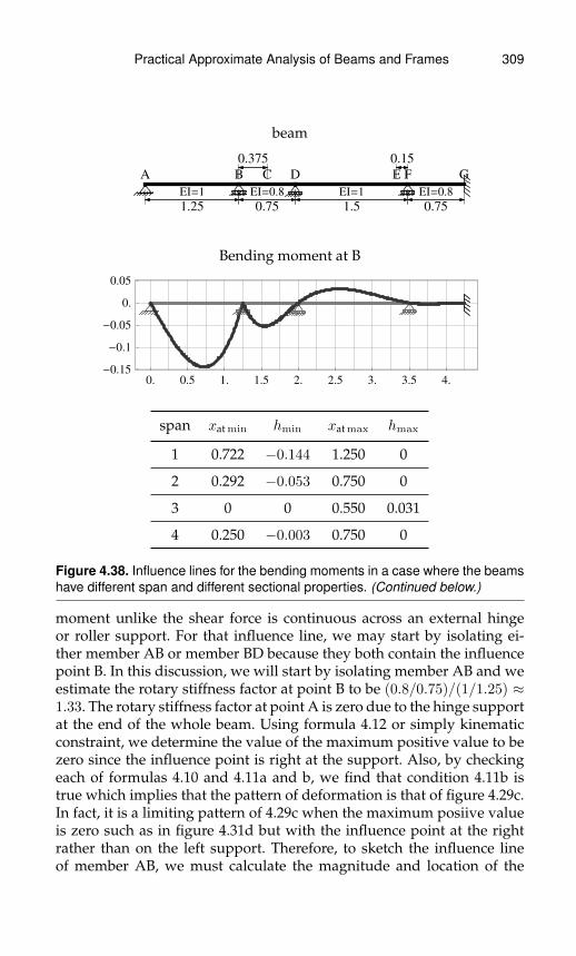
Practical Approximate Analysis of Beams and Frames 309
beam
1.25
EI=1
0.75
EI=0.8
0.375
1.5
EI=1
0.15
0.75
EI=0.8
A B C D E F G
Bending moment at B
0. 0.5 1. 1.5 2. 2.5 3. 3.5 4.
-0.15
-0.1
-0.05
0.
0.05
span xat min hmin xat max hmax
1 0.722 −0.144 1.250 0
2 0.292 −0.053 0.750 0
3 0 0 0.550 0.031
4 0.250 −0.003 0.750 0
Figure 4.38. Influence lines for the bending moments in a case where the beamshave different span and different sectional properties. (Continued below.)
moment unlike the shear force is continuous across an external hingeor roller support. For that influence line, we may start by isolating ei-ther member AB or member BD because they both contain the influencepoint B. In this discussion, we will start by isolating member AB and weestimate the rotary stiffness factor at point B to be (0.8/0.75)/(1/1.25) ≈1.33. The rotary stiffness factor at point A is zero due to the hinge supportat the end of the whole beam. Using formula 4.12 or simply kinematicconstraint, we determine the value of the maximum positive value to bezero since the influence point is right at the support. Also, by checkingeach of formulas 4.10 and 4.11a and b, we find that condition 4.11b istrue which implies that the pattern of deformation is that of figure 4.29c.In fact, it is a limiting pattern of 4.29c when the maximum posiive valueis zero such as in figure 4.31d but with the influence point at the rightrather than on the left support. Therefore, to sketch the influence lineof member AB, we must calculate the magnitude and location of the

310 Practical Approximate Analysis of Beams and Frames
Bending moment at C
0. 0.5 1. 1.5 2. 2.5 3. 3.5 4.
-0.1
-0.05
0.
0.05
0.1
0.15
span xat min hmin xat max hmax
1 0.722 −0.057 1.250 0
2 0 0 0.375 0.138
3 0.550 −0.058 1.500 0
4 0 0 0.250 0.005
Bending moment at E
0. 0.5 1. 1.5 2. 2.5 3. 3.5 4.
-0.1
-0.05
0.
0.05
0.1
span xat min hmin xat max hmax
1 0.722 −0.006 1.250 0
2 0 0 0.458 0.011
3 0.753 −0.070 1.350 0.061
4 0.250 −0.035 0.750 0
Figure 4.38. (Continued from above and continued below.)

Practical Approximate Analysis of Beams and Frames 311
Bending moment at G
0. 0.5 1. 1.5 2. 2.5 3. 3.5 4.
-0.15
-0.1
-0.05
0.
0.05
0.1
span xat min hmin xat max hmax
1 0 0 0.722 0.005
2 0.458 −0.009 0.750 0
3 0 0 0.944 0.080
4 0.457 −0.131 0.750 0
Figure 4.38. (Continued from above.) Influence lines for the bending moments ina case where the beams have different span and different sectional properties.
minimum over that member. Using formulas 4.14 and 4.15, we calcu-late those values to be 0.143 and 0.725 respectively. These values com-pare well with the exact results which are 0.144 (ie. about 0.69% error)and 0.722 (ie. about 0.42% error). At this point, we use the calculated val-ues to sketch the influence line for member AB using figure 4.29c andfigures 4.31 as a guide. To proceed further, we use formula 4.16b to cal-culate the slope at B to be 0.361. Note that there are two slopes at B dueto the kink and that the calculated slope is to the right of point B whichis the slope to be imposed on the member attached to the right of B. Thatmember is BD which is modeled as a transition member with the rotarystiffness factor at D estimated as (1/1.5)/(0.8/0.75) ≈ 0.625. With thatvalue of stiffness factor and an imposed slope at B of 0.361, we use for-mulas 4.18 and 4.19 to get the magnitude and location of the maximuminfluence in member BD to be 0.047 and 0.289 respectively. These valuesare close to the exact results of 0.053 (ie. about 11.3% error) and 0.292(ie. about 1.03% error) respectively. With these values, member BD canbe sketched using figure 4.32 as a guide (also see chapter 1). Consideringmember BD, we can also calculate the slope at D using 4.17 which gives aslope of 0.111. This slope is then imposed at point D of member DF withthe model of figure 4.32 in order to calculate values and to sketch theinfluence line for member DF. A similar procedure is again done for to

312 Practical Approximate Analysis of Beams and Frames
calculate basic values and to sketch the final member FG. This then com-pletes the sketch for the whole influence line for the bending momentat B and includes relatively accurate approximations of maxima, minimaand their locations.
Again considering figure 4.38, we next describe how to approxi-mately construct the influence line for the bending moment at C. Forthat influence line, we start by isolating member BD which is the mem-ber containing the influence point C. For that member BD, we estimatethe rotary stiffness factor at the left and right to be 0.75 and 0.625 respec-tively. Next, using formula 4.12, we calculate the value of the maximumpositive value which always occurs at the point of influence to be 0.133which compares well with the exact value of 0.138 (ie. about 3.6%). Atthis point, we have to determine the shape pattern of the influence lineover that member. We may do that by checking each of formulas 4.10and 4.11a and b where we find that condition 4.10 is true which im-plies that the pattern of deformation is that of figure 4.29a. This alsomeans that there are no negative values and we can proceed to sketchthe influence line over that member using figure 4.29a, figures 4.30 andfigures 4.31 as a guide. To proceed further, we calculate the slopes at Band D using formula 4.16a and b which give the values of 0.205 and 0.217respectively. These slopes are then used as imposed values on transitionmembers on the left and the right. For member AB on the left, the ro-tary stiffness factor at B is zero because of the free hinged end. Usingformula 4.18 and 4.19 with the imposed slope of 0.205, we get a maxi-mum value and location of 0.049 and 0.525 from the right (ie. 0.725 fromthe left) respectively which compare well with the exact results of 0.057(ie. about 14% error) and 0.722 (ie. about 0.42% error) respectively. Basedon these calculations for member AB, we can quantitatively sketch itsinfluence line using figure 4.32 as a guide (also see chapter1). For mem-ber DF on the left of the member with the influence point, we have animposed slope of 0.217 and we estimate the stiffness factor at point F tobe 1.6. Using formula 4.18 and 4.19 for member DF, we get a maximumvalue and location of 0.054 and 0.547 respectively which compare wellwith the exact results of 0.058 (ie. about 6.9% error) and 0.550 (ie. about0.55% error) respectively. Based on these calculations for member CE, wecan quantitatively sketch its influence line using figure 4.32 as a guide(also see chapter 1). To finish with member DF, we obtain the slope at Cusing formula 4.17 which gives a value of about 0.042. This slope is im-posed on member FG at point F and allows us to calculate basic valuesfor member FG and to sketch its influence line. This then would completethe whole sketch of the influence line for the bending moment at C. Thissketch includes relatively accurate approximations of maxima, minimaand their locations.

Appendix A
Beams—End-Momentsand Inflection Points
A.1 Moment End-Loaded Beam
EI
L
ΘnearΘfar
Mnear k ´ 4EI
L
L - xInflection
x
umax
xat max
krotary spring stiffness at near =Mnear
θnear=
3 + 4k
4 + 4k× 4× EI
L
⇔ krotary stiffness factor at near =Mnear
4× EILθnear
=3 + 4k
4 + 4k
krotary spring stiffness at near =3xinflection
6xinflection − 2
where: xinflection =xinflection
L(for 0 ≤ xinflection ≤ 1)
carry-over-moment =Mfar
Mnear=
2k
3 + 4k
1− xinflectionL =
2k
3 + 6k
313
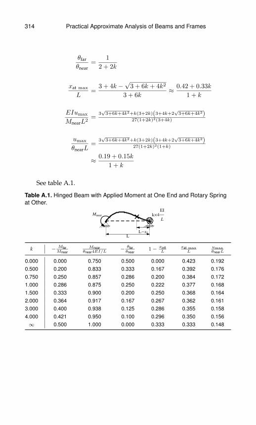
314 Practical Approximate Analysis of Beams and Frames
θfar
θnear=
1
2 + 2k
xat max
L=
3 + 4k −√
3 + 6k + 4k2
3 + 6k≈ 0.42 + 0.33k
1 + k
EIumax
MnearL2=
3√
3+6k+4k2+k(3+2k)(3+4k+2√
3+6k+4k2)27(1+2k)2(3+4k)
umax
θnearL=
3√
3+6k+4k2+k(3+2k)(3+4k+2√
3+6k+4k2)27(1+2k)2(1+k)
≈ 0.19 + 0.15k
1 + k
See table A.1.
Table A.1. Hinged Beam with Applied Moment at One End and Rotary Springat Other.
Mnear k´4
EI
L
L
L-xI
k − MfarMnear
Mnearθnear4EI/L
− θfarθnear
1− xinflL
xat maxL
umaxθnearL
0.000 0.000 0.750 0.500 0.000 0.423 0.1920.500 0.200 0.833 0.333 0.167 0.392 0.1760.750 0.250 0.857 0.286 0.200 0.384 0.1721.000 0.286 0.875 0.250 0.222 0.377 0.1681.500 0.333 0.900 0.200 0.250 0.368 0.1642.000 0.364 0.917 0.167 0.267 0.362 0.1613.000 0.400 0.938 0.125 0.286 0.355 0.1584.000 0.421 0.950 0.100 0.296 0.350 0.156∞ 0.500 1.000 0.000 0.333 0.333 0.148

Practical Approximate Analysis of Beams and Frames 315
A.2 Uniformly Distributed Load
EI
L
qkL
EI
L
kR
EI
L
kL ´ 4
EI
L
kR ´ 4
EI
L
xInf Left
xInf Right
MLeft
Min max
Mright
kL ´ 4
EI
L
kR ´ 4
EI
L
(a) (b) (c)
xinf left
L=
9 + 9kR + 3kL(5 + 4kR)
z
−√
3√
27(1+kR)2+k2L(27+8kR(5+2kR))+kL(54+10kR(9+4kR))
z
≈ 0.92kL3 + 4kL
where z = 6(3 + 4kR + 4kL(1 + kR)
)xinf right
L=
9 + 9kR + 3kL(5 + 4kR)
z
+√
3√
27(1+kR)2+k2L(27+8kR(5+2kR))+kL(54+10kR(9+4kR))
z
≈ 1− 0.92kR3+4kR
where z = 6(3 + 4kR + 4kL(1 + kR)
)Mleft
qL2/8= − 4kL(3 + 2kR)
9 + 12kL + 12kR + 12kL kR
Mright
qL2/8= − 4(3 + 2kL)kR
9 + 12kL + 12kR + 12kL kR
Min max
qL2/8=
27(1+kR)2+k2L(27+8kR(5+2kR))+kL(54+10kR(9+4kR))3(3+4kR+4kL(1+kR))2
≈(
1− 0.92kL3 + 4kL
− 0.92kR3 + 4kR
)2
EI × θnear
qL3= − 6 + kR
144 + 48kL + 48kR + 12kL kR
EI × θfar
qL3=
6 + kL144 + 48kL + 48kR + 12kL kR
See tables A.2 through A.4.
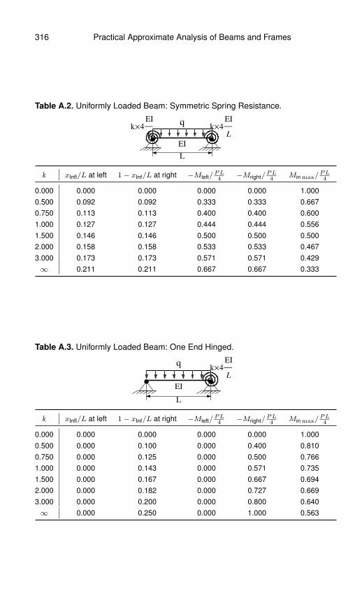
316 Practical Approximate Analysis of Beams and Frames
Table A.2. Uniformly Loaded Beam: Symmetric Spring Resistance.
EI
L
qk´4
EI
L
k´4
EI
L
k xInfl/L at left 1− xInf/L at right −Mleft/PL4
−Mright/PL4
Min max/PL4
0.000 0.000 0.000 0.000 0.000 1.0000.500 0.092 0.092 0.333 0.333 0.6670.750 0.113 0.113 0.400 0.400 0.6001.000 0.127 0.127 0.444 0.444 0.5561.500 0.146 0.146 0.500 0.500 0.5002.000 0.158 0.158 0.533 0.533 0.4673.000 0.173 0.173 0.571 0.571 0.429∞ 0.211 0.211 0.667 0.667 0.333
Table A.3. Uniformly Loaded Beam: One End Hinged.
EI
L
qk´4
EI
L
k xInfl/L at left 1− xInf/L at right −Mleft/PL4
−Mright/PL4
Min max/PL4
0.000 0.000 0.000 0.000 0.000 1.0000.500 0.000 0.100 0.000 0.400 0.8100.750 0.000 0.125 0.000 0.500 0.7661.000 0.000 0.143 0.000 0.571 0.7351.500 0.000 0.167 0.000 0.667 0.6942.000 0.000 0.182 0.000 0.727 0.6693.000 0.000 0.200 0.000 0.800 0.640∞ 0.000 0.250 0.000 1.000 0.563

Practical Approximate Analysis of Beams and Frames 317
Table A.4. Uniformly Loaded Beam: One End Fixed.
EI
L
qk´4
EI
L
k xInfl/L at left 1− xInf/L at right −Mleft/PL4
−Mright/PL4
Min max/PL4
0.000 0.250 0.000 1.000 0.000 0.5630.500 0.240 0.073 0.889 0.222 0.4720.750 0.236 0.094 0.857 0.286 0.4491.000 0.234 0.109 0.833 0.333 0.4321.500 0.230 0.130 0.800 0.400 0.4102.000 0.227 0.144 0.778 0.444 0.3963.000 0.223 0.161 0.750 0.500 0.379∞ 0.211 0.211 0.667 0.667 0.333
A.3 Point Force
PkL ´ 4
EI
L
kR ´ 4
EI
L
xF
kL ´ 4
EI
L
kR ´ 4
EI
L
xInf Left xInf Right
xF
MLeft
Min max
Mright
kL ´ 4
EI
L
kR ´ 4
EI
L
xF
(a) (b) (c)
xF = xF /L
xinf left
L= 2kL xF (2+2kR−(1+2kR)xF )
3+4kL+4kR+4kL kR+(4kL−2kR+4kL kR)xF−(2kL+2kR+8kL kR)x2F
≈ 3kL xF(2 + 4kL)(1 + xF )
xinf right
L=
3 + 4kR + (6kL + 8kL kR)xF − (2kL + 4kL kR)x2F
3 + 6kR + (6kL + 12kL kR)xF − (2kL + 2kR + 8kL kR)x2F
≈ 1− 3kR(1− xF )
(2 + 4kR)(2− xF )
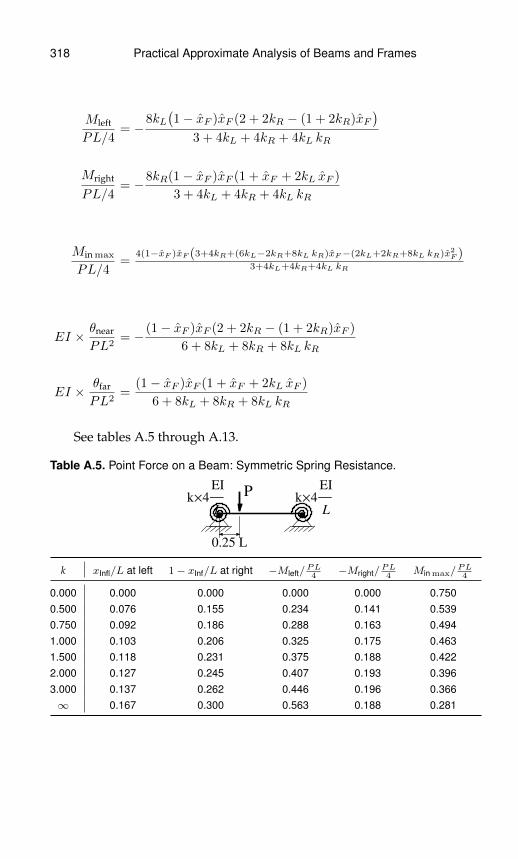
318 Practical Approximate Analysis of Beams and Frames
Mleft
PL/4= −
8kL(1− xF )xF (2 + 2kR − (1 + 2kR)xF
)3 + 4kL + 4kR + 4kL kR
Mright
PL/4= −8kR(1− xF )xF (1 + xF + 2kL xF )
3 + 4kL + 4kR + 4kL kR
Min max
PL/4=
4(1−xF )xF (3+4kR+(6kL−2kR+8kL kR)xF−(2kL+2kR+8kL kR)x2F )
3+4kL+4kR+4kL kR
EI × θnear
PL2= − (1− xF )xF (2 + 2kR − (1 + 2kR)xF )
6 + 8kL + 8kR + 8kL kR
EI × θfar
PL2=
(1− xF )xF (1 + xF + 2kL xF )
6 + 8kL + 8kR + 8kL kR
See tables A.5 through A.13.
Table A.5. Point Force on a Beam: Symmetric Spring Resistance.
Pk´4
EI
L
k´4
EI
L
0.25 L
k xInfl/L at left 1− xInf/L at right −Mleft/PL4
−Mright/PL4
Min max/PL4
0.000 0.000 0.000 0.000 0.000 0.7500.500 0.076 0.155 0.234 0.141 0.5390.750 0.092 0.186 0.288 0.163 0.4941.000 0.103 0.206 0.325 0.175 0.4631.500 0.118 0.231 0.375 0.188 0.4222.000 0.127 0.245 0.407 0.193 0.3963.000 0.137 0.262 0.446 0.196 0.366∞ 0.167 0.300 0.563 0.188 0.281
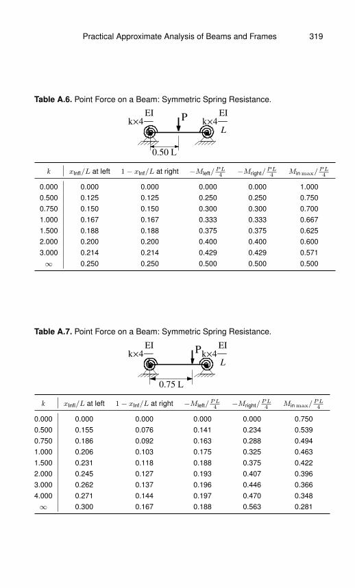
Practical Approximate Analysis of Beams and Frames 319
Table A.6. Point Force on a Beam: Symmetric Spring Resistance.
Pk´4
EI
L
k´4
EI
L
0.50 L
k xInfl/L at left 1− xInf/L at right −Mleft/PL4
−Mright/PL4
Min max/PL4
0.000 0.000 0.000 0.000 0.000 1.0000.500 0.125 0.125 0.250 0.250 0.7500.750 0.150 0.150 0.300 0.300 0.7001.000 0.167 0.167 0.333 0.333 0.6671.500 0.188 0.188 0.375 0.375 0.6252.000 0.200 0.200 0.400 0.400 0.6003.000 0.214 0.214 0.429 0.429 0.571∞ 0.250 0.250 0.500 0.500 0.500
Table A.7. Point Force on a Beam: Symmetric Spring Resistance.
Pk´4
EI
L
k´4
EI
L
0.75 L
k xInfl/L at left 1− xInf/L at right −Mleft/PL4
−Mright/PL4
Min max/PL4
0.000 0.000 0.000 0.000 0.000 0.7500.500 0.155 0.076 0.141 0.234 0.5390.750 0.186 0.092 0.163 0.288 0.4941.000 0.206 0.103 0.175 0.325 0.4631.500 0.231 0.118 0.188 0.375 0.4222.000 0.245 0.127 0.193 0.407 0.3963.000 0.262 0.137 0.196 0.446 0.3664.000 0.271 0.144 0.197 0.470 0.348∞ 0.300 0.167 0.188 0.563 0.281
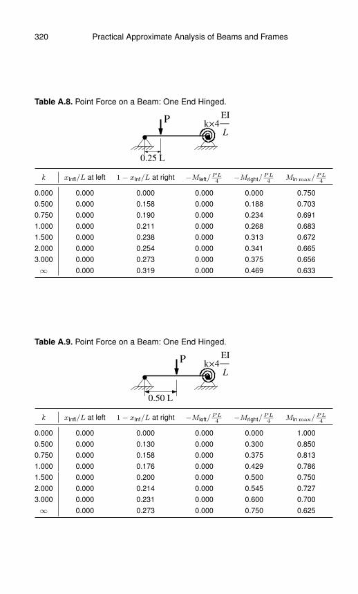
320 Practical Approximate Analysis of Beams and Frames
Table A.8. Point Force on a Beam: One End Hinged.
Pk´4
EI
L
0.25 L
k xInfl/L at left 1− xInf/L at right −Mleft/PL4
−Mright/PL4
Min max/PL4
0.000 0.000 0.000 0.000 0.000 0.7500.500 0.000 0.158 0.000 0.188 0.7030.750 0.000 0.190 0.000 0.234 0.6911.000 0.000 0.211 0.000 0.268 0.6831.500 0.000 0.238 0.000 0.313 0.6722.000 0.000 0.254 0.000 0.341 0.6653.000 0.000 0.273 0.000 0.375 0.656∞ 0.000 0.319 0.000 0.469 0.633
Table A.9. Point Force on a Beam: One End Hinged.
Pk´4
EI
L
0.50 L
k xInfl/L at left 1− xInf/L at right −Mleft/PL4
−Mright/PL4
Min max/PL4
0.000 0.000 0.000 0.000 0.000 1.0000.500 0.000 0.130 0.000 0.300 0.8500.750 0.000 0.158 0.000 0.375 0.8131.000 0.000 0.176 0.000 0.429 0.7861.500 0.000 0.200 0.000 0.500 0.7502.000 0.000 0.214 0.000 0.545 0.7273.000 0.000 0.231 0.000 0.600 0.700∞ 0.000 0.273 0.000 0.750 0.625

Practical Approximate Analysis of Beams and Frames 321
Table A.10. Point Force on a Beam: One End Hinged.
Pk´4
EI
L
0.75 L
k xInfl/L at left 1− xInf/L at right −Mleft/PL4
−Mright/PL4
Min max/PL4
0.000 0.000 0.000 0.000 0.000 0.7500.500 0.000 0.080 0.000 0.263 0.5530.750 0.000 0.099 0.000 0.328 0.5041.000 0.000 0.111 0.000 0.375 0.4691.500 0.000 0.127 0.000 0.437 0.4222.000 0.000 0.137 0.000 0.477 0.3923.000 0.000 0.149 0.000 0.525 0.356∞ 0.000 0.179 0.000 0.656 0.258
Table A.11. Point Force on a Beam: One End Fixed.
Pk´4
EI
L
0.25 L
k xInfl/L at left 1− xInf/L at right −Mleft/PL4
−Mright/PL4
Min max/PL4
0.000 0.179 0.000 0.656 0.000 0.2580.500 0.175 0.143 0.625 0.063 0.2660.750 0.174 0.173 0.616 0.080 0.2681.000 0.173 0.194 0.609 0.094 0.2701.500 0.172 0.220 0.600 0.113 0.2722.000 0.171 0.235 0.594 0.125 0.2733.000 0.170 0.254 0.586 0.141 0.275∞ 0.167 0.300 0.562 0.188 0.281
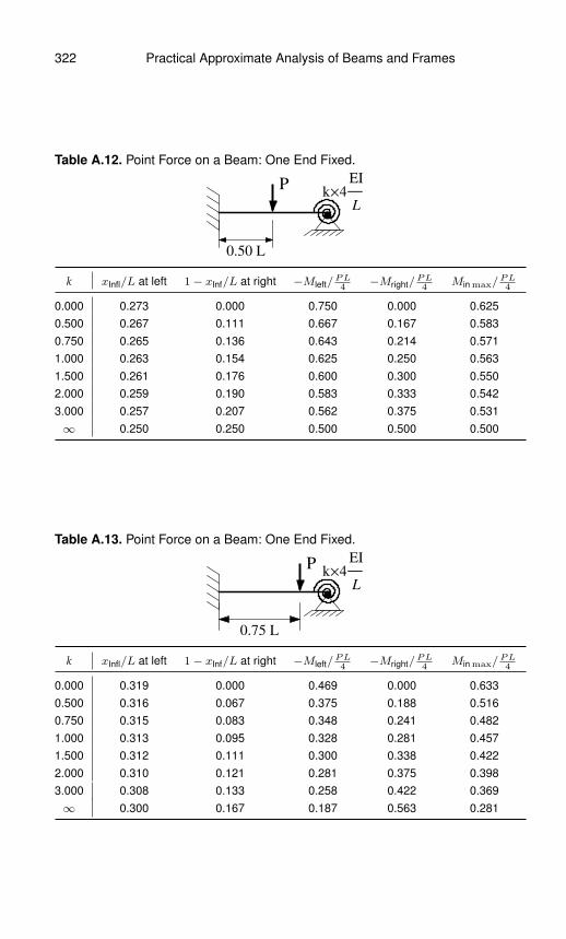
322 Practical Approximate Analysis of Beams and Frames
Table A.12. Point Force on a Beam: One End Fixed.
Pk´4
EI
L
0.50 L
k xInfl/L at left 1− xInf/L at right −Mleft/PL4
−Mright/PL4
Min max/PL4
0.000 0.273 0.000 0.750 0.000 0.6250.500 0.267 0.111 0.667 0.167 0.5830.750 0.265 0.136 0.643 0.214 0.5711.000 0.263 0.154 0.625 0.250 0.5631.500 0.261 0.176 0.600 0.300 0.5502.000 0.259 0.190 0.583 0.333 0.5423.000 0.257 0.207 0.562 0.375 0.531∞ 0.250 0.250 0.500 0.500 0.500
Table A.13. Point Force on a Beam: One End Fixed.
Pk´4
EI
L
0.75 L
k xInfl/L at left 1− xInf/L at right −Mleft/PL4
−Mright/PL4
Min max/PL4
0.000 0.319 0.000 0.469 0.000 0.6330.500 0.316 0.067 0.375 0.188 0.5160.750 0.315 0.083 0.348 0.241 0.4821.000 0.313 0.095 0.328 0.281 0.4571.500 0.312 0.111 0.300 0.338 0.4222.000 0.310 0.121 0.281 0.375 0.3983.000 0.308 0.133 0.258 0.422 0.369∞ 0.300 0.167 0.187 0.563 0.281

Appendix B
Column—ShearStiffness, End-Momentsand Inflection Points
B.1 Cantilever
k ´ 4
EI
L
P
Mapp
L
EI
Deflection of a cantilever:
δ =
(1
2+
1
4k
)L2
EIMapp +
(1
3+
1
4k
)L2
EIPL
Shear stiffness:
ksh =4k(
(6k + 3)Mapp
PL+ (4k + 3)
) 3EI
L3
If k =∞ (fixed support):
ksh =4(
6Mapp
PL + 4) 3EI
L3
If k =∞ (fixed support) and Mapp = 0:
ksh =3EI
L3
323

324 Practical Approximate Analysis of Beams and Frames
B.2 Column for Single Story Building
k ´ 4
EI
LP
LEI
k ´ 4
EI
LP
LEI
hinge support fixed support
Shear stiffness:
ksh =
4k
(3+4k)3EIL3 (hinge support)
(1+4k)(4+4k)
12EIL3 (fixed support)
0 (roller support)
Moment at top and bottom of column:(Minner top
Minner bottom
)=
(2k
1+4k
− (1+2k)(1+4k)
)PL (fixed support)
and (Minner top
Minner bottom
)=
(1
0
)PL (hinged support)
Inflection point measured from the bottom:
xI =(1 + 2k)
(1 + 4k)L (fixed support)
Note that in the above formulas, the inner bending momentsMinner top and Minner bottom are considered to be positive when counter-clockwise and clockwise respectively in conformance with standard con-ventions of bending moment diagrams.
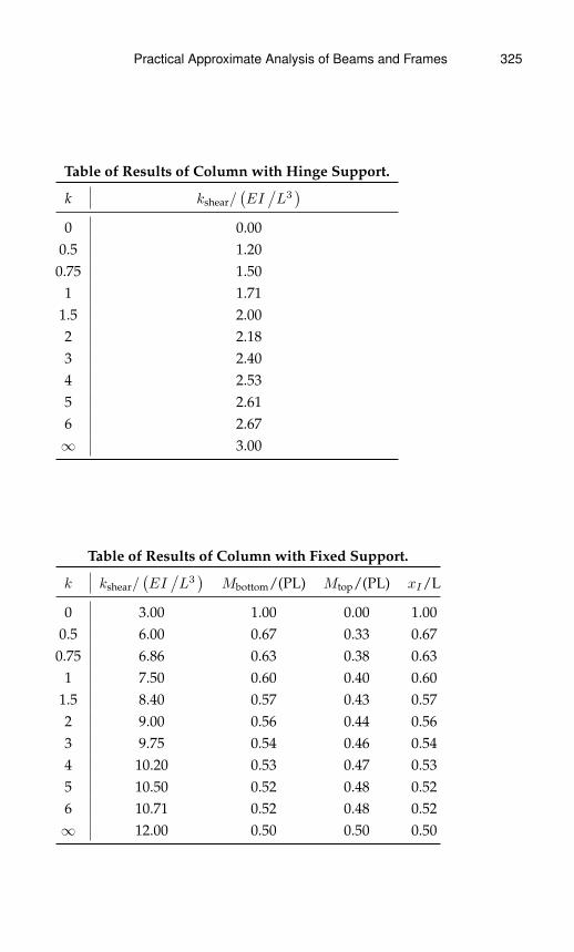
Practical Approximate Analysis of Beams and Frames 325
Table of Results of Column with Hinge Support.
k kshear/(EI/L3)
0 0.000.5 1.200.75 1.50
1 1.711.5 2.002 2.183 2.404 2.535 2.616 2.67∞ 3.00
Table of Results of Column with Fixed Support.
k kshear/(EI/L3)
Mbottom/(PL) Mtop/(PL) xI/L
0 3.00 1.00 0.00 1.000.5 6.00 0.67 0.33 0.670.75 6.86 0.63 0.38 0.63
1 7.50 0.60 0.40 0.601.5 8.40 0.57 0.43 0.572 9.00 0.56 0.44 0.563 9.75 0.54 0.46 0.544 10.20 0.53 0.47 0.535 10.50 0.52 0.48 0.526 10.71 0.52 0.48 0.52∞ 12.00 0.50 0.50 0.50

326 Practical Approximate Analysis of Beams and Frames
B.3 Column for Multi-StoryBuilding—First Floor
kt´4EI
L
MtP
xI
L
kt´4EI
L
MtP
L
Shear stiffness:
ksh =
1+4kt(4+4kt)+6(Mt/(PL))
12EIL3 (fixed)
4kt(3+4kt)+3(Mt/(PL))
3EIL3 (hinge)
Moment at top and bottom of column for fixed support:
(Minner top
Minner bottom
)=
(+ 2kt
1+4kt
−1+2kt1+4kt
)PL+
(− 1
1+4kt
− 11+4kt
)Mt (fixed support)(
1
0
)PL (hinged support)
Inflection point measured from the bottom (for fixed support):
xI = (1+2kt)+(Mt/(PL))(1+4kt)
L (on condition 0 ≤ xI ≤ L)
Note that in the above formulas, the applied moment Mt is consid-ered positive when clockwise and the applied load P is considered pos-itive when acting to the right. By contrast, the inner bending momentsMinner top and Minner bottom are considered to be positive when counter-clockwise and clockwise respectively in conformance with standard con-ventions of bending moment diagrams.
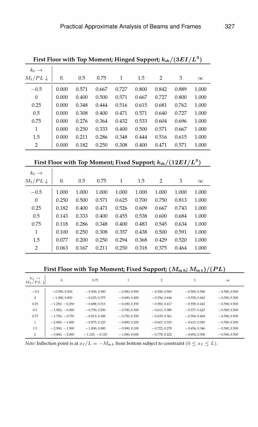
Practical Approximate Analysis of Beams and Frames 327
First Floor with Top Moment; Hinged Support; ksh/(3EI/L3)
kt →Mt/PL ↓ 0. 0.5 0.75 1 1.5 2 3 ∞
−0.5 0.000 0.571 0.667 0.727 0.800 0.842 0.889 1.0000 0.000 0.400 0.500 0.571 0.667 0.727 0.800 1.000
0.25 0.000 0.348 0.444 0.516 0.615 0.681 0.762 1.0000.5 0.000 0.308 0.400 0.471 0.571 0.640 0.727 1.000
0.75 0.000 0.276 0.364 0.432 0.533 0.604 0.696 1.0001 0.000 0.250 0.333 0.400 0.500 0.571 0.667 1.000
1.5 0.000 0.211 0.286 0.348 0.444 0.516 0.615 1.0002 0.000 0.182 0.250 0.308 0.400 0.471 0.571 1.000
First Floor with Top Moment; Fixed Support; ksh/(12EI/L3)
kt →Mt/PL ↓ 0. 0.5 0.75 1 1.5 2 3 ∞
−0.5 1.000 1.000 1.000 1.000 1.000 1.000 1.000 1.0000 0.250 0.500 0.571 0.625 0.700 0.750 0.813 1.000
0.25 0.182 0.400 0.471 0.526 0.609 0.667 0.743 1.0000.5 0.143 0.333 0.400 0.455 0.538 0.600 0.684 1.000
0.75 0.118 0.286 0.348 0.400 0.483 0.545 0.634 1.0001 0.100 0.250 0.308 0.357 0.438 0.500 0.591 1.000
1.5 0.077 0.200 0.250 0.294 0.368 0.429 0.520 1.0002 0.063 0.167 0.211 0.250 0.318 0.375 0.464 1.000
First Floor with Top Moment; Fixed Support; (Min b;Min t)/(PL)
kt →Mt/PL ↓ 0. 0.75 1 2 3 ∞
−0.5 −0.500; 0.500 −0.500; 0.500 −0.500; 0.500 −0.500; 0.500 −0.500; 0.500 −0.500; 0.500
0 −1.000; 0.000 −0.625; 0.375 −0.600; 0.400 −0.556; 0.444 −0.538; 0.462 −0.500; 0.500
0.25 −1.250;−0.250 −0.688; 0.313 −0.650; 0.350 −0.583; 0.417 −0.558; 0.442 −0.500; 0.500
0.5 −1.500;−0.500 −0.750; 0.250 −0.700; 0.300 −0.611; 0.389 −0.577; 0.423 −0.500; 0.500
0.75 −1.750;−0.750 −0.813; 0.188 −0.750; 0.250 −0.639; 0.361 −0.596; 0.404 −0.500; 0.500
1 −2.000;−1.000 −0.875; 0.125 −0.800; 0.200 −0.667; 0.333 −0.615; 0.385 −0.500; 0.500
1.5 −2.500;−1.500 −1.000; 0.000 −0.900; 0.100 −0.722; 0.278 −0.654; 0.346 −0.500; 0.500
2 −3.000;−2.000 −1.125;−0.125 −1.000; 0.000 −0.778; 0.222 −0.692; 0.308 −0.500; 0.500
Note: Inflection point is at xI/L = −Min b from bottom subject to constraint (0 ≤ xI ≤ L).

328 Practical Approximate Analysis of Beams and Frames
B.4 Column for Multi-Story Building—Top Floor(Top and Bottom Beams Similar)
k´4EI
L
Mb
k´4EI
L
P
xI
L
Shear stiffness:
ksh =
(2k + 4k2
)(3 + 8k + 4k2) + 3(1 + 2k)(Mb/(PL)
12EI
L3
Moment at top and bottom of column:(Minner top
Minner bottom
)=
(+1
2
−12
)PL+
(+ 1
2+4k
+ 12+4k
)Mb
Inflection point measured from the bottom:
xI = 12 −
Mb/(PL)(2+4k) L (on condition 0 ≤ xI ≤ L)
Note that in the above formulas, the applied moment Mb is consid-ered positive when clockwise and the applied load P is considered pos-itive when acting to the right. By contrast, the inner bending momentsMinner top and Minner bottom are considered to be positive when counter-clockwise and clockwise respectively in conformance with standard con-ventions of bending moment diagrams.
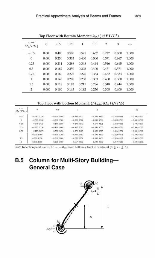
Practical Approximate Analysis of Beams and Frames 329
Top Floor with Bottom Moment; ksh/(12EI/L3)
k →Mb/PL ↓
0. 0.5 0.75 1 1.5 2 3 ∞
−0.5 0.000 0.400 0.500 0.571 0.667 0.727 0.800 1.000
0 0.000 0.250 0.333 0.400 0.500 0.571 0.667 1.000
0.25 0.000 0.211 0.286 0.348 0.444 0.516 0.615 1.000
0.5 0.000 0.182 0.250 0.308 0.400 0.471 0.571 1.000
0.75 0.000 0.160 0.222 0.276 0.364 0.432 0.533 1.000
1 0.000 0.143 0.200 0.250 0.333 0.400 0.500 1.000
1.5 0.000 0.118 0.167 0.211 0.286 0.348 0.444 1.000
2 0.000 0.100 0.143 0.182 0.250 0.308 0.400 1.000
Top Floor with Bottom Moment; (Min b;Min t)/(PL)
k →Mb/PL ↓ 0. 0.75 1 2 3 ∞
−0.5 −0.750; 0.250 −0.600; 0.400 −0.583; 0.417 −0.550; 0.450 −0.536; 0.464 −0.500; 0.500
0 −0.500; 0.500 −0.500; 0.500 −0.500; 0.500 −0.500; 0.500 −0.500; 0.500 −0.500; 0.500
0.25 −0.375; 0.625 −0.450; 0.550 −0.458; 0.542 −0.475; 0.525 −0.482; 0.518 −0.500; 0.500
0.5 −0.250; 0.750 −0.400; 0.600 −0.417; 0.583 −0.450; 0.550 −0.464; 0.536 −0.500; 0.500
0.75 −0.125; 0.875 −0.350; 0.650 −0.375; 0.625 −0.425; 0.575 −0.446; 0.554 −0.500; 0.500
1 0.000; 1.000 −0.300; 0.700 −0.333; 0.667 −0.400; 0.600 −0.429; 0.571 −0.500; 0.500
1.5 0.250; 1.250 −0.200; 0.800 −0.250; 0.750 −0.350; 0.650 −0.393; 0.607 −0.500; 0.500
2 0.500; 1.500 −0.100; 0.900 −0.167; 0.833 −0.300; 0.700 −0.357; 0.643 −0.500; 0.500
Note: Inflection point is at xI/L = −Min b from bottom subject to constraint (0 ≤ xI ≤ L).
B.5 Column for Multi-Story Building—General Case
kb´4EI
L
Mb
kt´4EI
L
MtP
xI
L

330 Practical Approximate Analysis of Beams and Frames
Shear stiffness:
ksh = kb+kt+4kbkt(3+4kb+4kt+4kbkt)+3(1+2kt)(Mb/(PL))+3(1+2kb)(Mt/(PL))
12EIL3
Moment at top and bottom of column:(Minner top
Minner bottom
)=
(+ kt+2kbktkb+kt+4kbkt
− kb+2kbktkb+kt+4kbkt
)PL+
(+ ktkb+kt+4kbkt
+ ktkb+kt+4kbkt
)Mb
+
(− kbkb+kt+4kbkt
− kbkb+kt+4kbkt
)Mt
Inflection point measured from the bottom:
xI = (kb+2kbkt)−kt(Mb/(PL))+kb(Mt/(PL))(kb+kt+4kbkt)
L
(on condition 0 ≤ xI ≤ L)
Note that in the above formulas, the applied moments Mt and Mb
are considered positive when clockwise and the applied load P is con-sidered positive when acting to the right. By contrast, the inner bendingmoments Minner top and Minner bottom are considered to be positive whencounterclockwise and clockwise respectively in conformance with stan-dard conventions of bending moment diagrams.
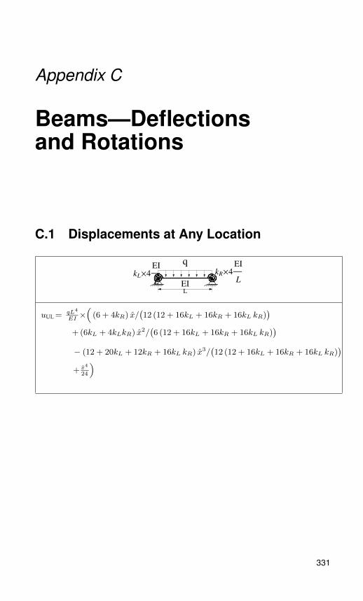
Appendix C
Beams—Deflectionsand Rotations
C.1 Displacements at Any Location
kL´4
EI
L
kR´4
EI
L
q
L
EI
uUL = qL4
EI×(
(6 + 4kR) x/(12 (12 + 16kL + 16kR + 16kL kR)
)+ (6kL + 4kLkR) x2/
(6 (12 + 16kL + 16kR + 16kL kR)
)− (12 + 20kL + 12kR + 16kL kR) x3/
(12 (12 + 16kL + 16kR + 16kL kR)
)+ x4
24
)
331

332 Practical Approximate Analysis of Beams and Frames
kL´4
EI
L
kR´4
EI
L
L
EI
PxF
uPF = PL3
EI×
(x (1 − xF )) / (18 + 24kL + 24kR + 24kL kR)((− (6 + 6kR) xF + (3 + 6kR) x2F
)+ (− (12kL + 12kL kR) xF
+ (6kL + 12kL kR) x2F
)x
+ ((3 + 4kL + 4kR + 4kL kR)
+ (4kL − 2kR + 4kL kR) xF
− (2kL + 2kR + 8kL kR) x2F)x2)
0 ≤ x < xF
((1 − x) xF ) / (18 + 24kL + 24kR + 24kL kR)((3 + 4kL + 4kR + 4kL kR) x2F
+ (− (6 + 6kR) − (12kL + 12kL kR) xF
+ (4kL − 2kR + 4kL kR) x2F)x
+ ((3 + 6kR) (6kL + 12kL kR) xF
− (2kL + 2kR + 8kL kR) x2F)x2)
xF ≤ x ≤ 1

Practical Approximate Analysis of Beams and Frames 333
kL´4
EI
L
kR´4
EI
L
L
EI
MxF
uM = ML2
EI×
x/ (6 + 8kL + 8kR + 8kL kR)
((− (2 + 2kR)
+ (6 + 8kR) xF − (3 + 6kR) x2F)
+ (− (4kL + 4kL kR)
+ (12kL + 16kL kR) xF
− (6kL + 12kL kR) x2F)x
+ (− (1 + 2kR) − (4kL + 8kL kR) xF
− (2kL + 2kR + 8kL kR) x2F
)x2)
0 ≤ x < xF
(1 − x) /(6 + 8kL + 8kR + 8kL kR)
((3 + 4kL + 4kR + 4kL kR) x2F
+ (− (2 + 2kR) − (8kL + 8kL kR) xF
+ (4kL − 2kR + 4kL kR) x2F)x
+ ((1 + 2kR) + (4kL + 8kL kR) xF
− (2kL + 2kR + 8kL kR) x2F
)x2)
xF ≤ x ≤ 1
Note:
• x = x/L
• xF = xF /L

334 Practical Approximate Analysis of Beams and Frames
C.2 Rotations at Any Location
kL´4
EI
L
kR´4
EI
L
q
L
EI
θUL = 6+kRz
+ 6kL+kL kRz
x− 36+15kL+9kR+3kL kRz
x2
+24+8kL+8kR+2kL kR1z x3
z = 144 + 48kL + 48kR + 12kL kR
kL´4
EI
L
kR´4
EI
L
L
EI
PxF
θPF =
(2+2kR)xF−(3+4kR)x2F +(1+2kR)x3
F
6+8kL+8kR+8kL kR
+(8kL+8kL kR)xF−(12kL+16kL kR)x2
F
6+8kL+8kR+8kL kRx
+(4kL+8kL kR)x3
F
6+8kL+8kR+8kL kRx
+−(3+4kL+4kR+4kL kR)+(3+6kR)xF
6+8kL+8kR+8kL kR
+(6kL+12kL kR)x2
F−(2kL+2kR+8kL kR)x3F
6+8kL+8kR+8kL kR
0 ≤ x ≤ xF
(2+2kR)xF +(4kL+4kL kR)x2F +(1+2kR)x3
F
6+8kL+8kR+8kL kR
+−(6+8kR)xF−(12kL+16kL kR)x2
F
6+8kL+8kR+8kL kRx
+(4kL+8kL kR)x3
F
6+8kL+8kR+8kL kRx
+(3+6kR)xF +(6kL+12kL kR)x2
F
6+8kL+8kR+8kL kRx2
− (2kL+2kR+8kL kR)x3F
6+8kL+8kR+8kL kRx2
xF < x ≤ 1

Practical Approximate Analysis of Beams and Frames 335
kL´4
EI
L
kR´4
EI
L
L
EI
MappxF
θPM =
2+2kR+(−6−8kR)xF +(3+6kR)x2F
6+8kL+8kR+8kL kR
+ 8kL+8kL kR−(32kL kR+24kL)xF
6+8kL+8kR+8kL kRx
+(12kL+24kL kR)x2
F
6+8kL+8kR+8kL kRx
+ (3+6kR)+(12kL+24kLkR)xF
6+8kL+8kR+8kL kRx2
− (24kL kR+6kL+6kR)x2F
6+8kL+8kR+8kL kRx2
0 ≤ x ≤ xF
2+2kR+(8kL+8kL kR)xF +(3+6kR)x2F
6+8kL+8kR+8kL kR
+−(8kR+6)−(32kL kR+24kL)xF
6+8kL+8kR+8kL kRx
+(12kL+24kL kR)x2
F
6+8kL+8kR+8kL kRx
+ (3+6kR)+(12kL+24kL kR)xF
6+8kL+8kR+8kL kRx2
− (24kL kR+6kL+6kR)x2F
6+8kL+8kR+8kL kRx2
xF < x ≤ 1
Note:
• x = x/L
• xF = xF /L
• Rotations are clockwise when positive
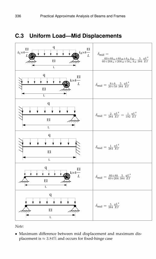
336 Practical Approximate Analysis of Beams and Frames
C.3 Uniform Load—Mid Displacements
kL´4
EI
L
kR´4
EI
L
q
L
EI
δmid =60+8kL+8kR+kL kR
60+20kL+20kR+5kL kR5
384qL4
EI
k´4
EI
L
q
L
EI
δmid = 8+k20+5k
5384
qL4
EI
q
L
EI
δmid = 2384
qL4
EI = 1192
qL4
EI
q
L
EI
δmid = 1384
qL4
EI
k´4
EI
L
q
L
EI
δmid = 60+8k60+20k
5384
qL4
EI
q
L
EI
δmid = 5384
qL4
EI
Note:
• Maximum difference between mid displacement and maximum dis-placement is ≈ 3.84% and occurs for fixed-hinge case

Practical Approximate Analysis of Beams and Frames 337
• Continuous beam with equal spacing and only one member loadedobtained with kL ≈ kR ≈ 1 for mid member or k ≈ 1 for edge member
• Continuous beam with equal spacing and all members uniformlyloaded obtained with fixed-fixed case
• Continuous beam with equal spacing and checker-board loading ob-tained with kL ≈ kR ≈ 0.5 for mid member or k ≈ 0.5 for edgemember

338 Practical Approximate Analysis of Beams and Frames
C.4 Point Force—Centrally Loaded—Mid Displacements
0
kL´4
EI
L
kR´4
EI
L
L
EI
PL�2
δmid =12+7kL+7kR+4kL kR
12+16kL+16kR+16kL kR148PL3
EI
k´4
EI
L
L
EI
PL�2
δmid = 7+4k16+16k
148PL3
EI
L
EI
PL�2
δmid = 716
148PL3
EI = 7768
PL3
EI
L
EI
PL�2
δmid = 1192
PL3
EI
k´4
EI
L
L
EI
PL�2
δmid = 12+7k12+16k
148PL3
EI
L
EI
PL�2
δmid = 148PL3
EI

Practical Approximate Analysis of Beams and Frames 339
Note:
• Maximum difference between mid displacement and maximum dis-placement is ≈ 2.17% and occurs for fixed-hinge case
• For same total load (qL = P ), we have:
– fixed-fixed case of point load is 2 times that of distributed load
– fixed-hinge case of point load is 1.75 times that of distributed load
– hinge-hinge case of point load is 1.6 times that of distributed load
• Continuous beam with equal spacing and only one member loadedobtained with kL ≈ kR ≈ 1 for mid member or k ≈ 1 for edge member
• Continuous beam with equal spacing and all members uniformlyloaded obtained with fixed-fixed case
• Continuous beam with equal spacing and checker-board loading ob-tained with kL ≈ kR ≈ 0.5 for mid member or k ≈ 0.5 for edgemember
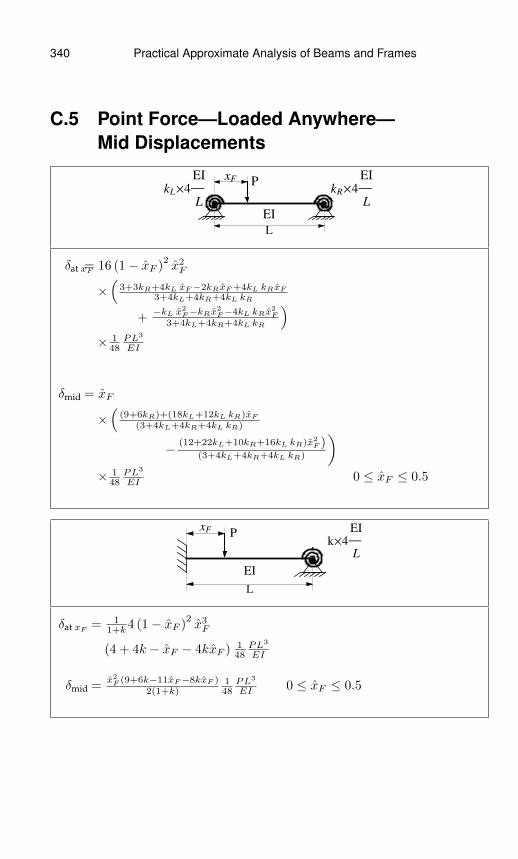
340 Practical Approximate Analysis of Beams and Frames
C.5 Point Force—Loaded Anywhere—Mid Displacements
kL´4
EI
L
kR´4
EI
L
L
EI
PxF
δat xF= 16 (1− xF )
2x2F
×(
3+3kR+4kL xF−2kRxF +4kL kRxF
3+4kL+4kR+4kL kR
+−kL x2
F−kRx2F−4kL kRx
2F
3+4kL+4kR+4kL kR
)× 1
48PL3
EI
δmid = xF
×(
(9+6kR)+(18kL+12kL kR)xF
(3+4kL+4kR+4kL kR)
− (12+22kL+10kR+16kL kR)x2F )
(3+4kL+4kR+4kL kR)
)× 1
48PL3
EI0 ≤ xF ≤ 0.5
k´4
EI
L
L
EI
PxF
δat xF= 1
1+k4 (1− xF )2x3F
(4 + 4k − xF − 4kxF ) 148PL3
EI
δmid =x2F (9+6k−11xF−8kxF )
2(1+k)148PL3
EI 0 ≤ xF ≤ 0.5

Practical Approximate Analysis of Beams and Frames 341
L
EI
PxF
δat xF = 4 (1− xF )2
(4− xF ) x3F
148PL3
EI
δmid = 12x2F (9− 11xF ) 1
48PL3
EI0 ≤ xF ≤ 0.5
L
EI
PxF
δat xF= 16(1− xF )3x3
F148PL3
EI
δmid = (3− 4xF )x2F
148PL3
EI 0 ≤ xF ≤ 0.5
k´4
EI
L
L
EI
PxF
δat xF= 1
3+4k16 (1− xF )2
x2F
(3 + 3k − 2kxF − kx2
F
)148PL3
EI
δmid =xF (9+6k−12x2
F−10kx2F )
3+4k148PL3
EI 0 ≤ xF ≤ 0.5
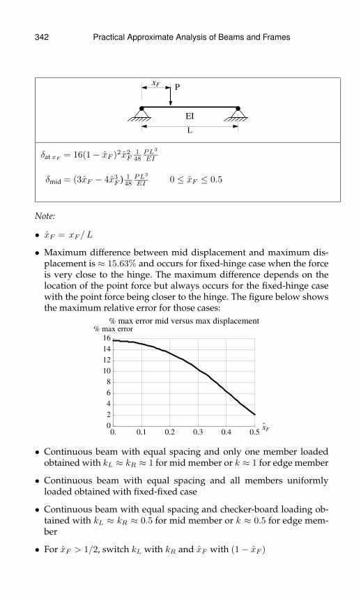
342 Practical Approximate Analysis of Beams and Frames
L
EI
PxF
δat xF= 16(1− xF )2x2
F148PL3
EI
δmid = (3xF − 4x3F ) 1
48PL3
EI0 ≤ xF ≤ 0.5
Note:
• xF = xF /L
• Maximum difference between mid displacement and maximum dis-placement is ≈ 15.63% and occurs for fixed-hinge case when the forceis very close to the hinge. The maximum difference depends on thelocation of the point force but always occurs for the fixed-hinge casewith the point force being closer to the hinge. The figure below showsthe maximum relative error for those cases:
0. 0.1 0.2 0.3 0.4 0.5x`
F0
2
4
6
8
10
12
14
16
% max error
% max error mid versus max displacement
• Continuous beam with equal spacing and only one member loadedobtained with kL ≈ kR ≈ 1 for mid member or k ≈ 1 for edge member
• Continuous beam with equal spacing and all members uniformlyloaded obtained with fixed-fixed case
• Continuous beam with equal spacing and checker-board loading ob-tained with kL ≈ kR ≈ 0.5 for mid member or k ≈ 0.5 for edge mem-ber
• For xF > 1/2, switch kL with kR and xF with (1− xF )

Practical Approximate Analysis of Beams and Frames 343
C.6 Point Moment—Loaded Anywhere—Mid Displacements
kL´4
EI
L
kR´4
EI
L
L
EI
MappxF
δat xF= 16 (1− xF ) xF
×(
1+kR−2xF +2kL xF−3kRxF +2kL kRxF
3+4kL+4kR+4kL kR
+−4kL x
2F +kRx
2F−6KLkR xF 2kL x
4F +4kL kR x
3F
3+4kL+4kR+4kL kR
)× 1
16ML2
EI
δmid=(
3+2kR+12kLxF +8kL kRxF−12x2F
3+4kL+4kR+4kL kR
+−22kLx
2F−10kRx
2F−16kL kR x
2F
3+4kL+4kR+4kL kR
)× 1
16ML2
EI0 ≤ xF ≤ 0.5
k´4
EI
L
L
EI
MappxF
δat xF= 4 (1− xF ) x2
F
× (2+2k−4xF−6kxF +x2F +4kx2
F )1+k
× 116ML3
EI
δmid = (64k−11xF−8kxF )xF
2(1+k)116ML3
EI 0 ≤ xF ≤ 0.5
L
EI
MappxF
δat xF= 4 (1− xF ) x2
F
(2− 4xF + x2
F
)116ML2
EI
δmid = 12 (6− 11xF ) xF
116ML2
EI 0 ≤ xF ≤ 0.5

344 Practical Approximate Analysis of Beams and Frames
L
EI
MappxF
δat xF= 8 (1− xF ) x2
F
(1− 3xF + 2x2
F
)116ML2
EI
δmid = 2 (1− 2xF ) 116ML2
EI0 ≤ xF ≤ 0.5
k´4
EI
L
L
EI
MappxF
δat xF=
16(1−xF )xF (1+k−2xF−3kxF +kx2F +kx3
F )3+4k
× 116ML2
EI
δmid =3+2k−12x2
F−10kx2F
3+4k116ML2
EI 0 ≤ xF ≤ 0.5
L
EI
MappxF
δat xF= 16
3 (1− xF ) xF (1− 2xF ) 116ML2
EI
δmid = (1− 4xF ) 116ML2
EI 0 ≤ xF ≤ 0.5
Note:
• xF = xF /L
• In general, neither δat xFnor δmid is the maximum deflection
• Continuous beam with equal spacing and only one member loadedobtained with kL ≈ kR ≈ 1 for mid member or k ≈ 1 for edge member
Practical Approximate Analysis of Beams and Frames 345
• Continuous beam with equal spacing and all members uniformlyloaded obtained with fixed-fixed case
• Continuous beam with equal spacing and checker-board loading ob-tained with kL ≈ kR ≈ 0.5 for mid member or k ≈ 0.5 for edgemember
• For xF > 1/2, switch kL with kR and xF with (1− xF )
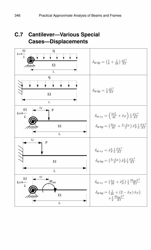
346 Practical Approximate Analysis of Beams and Frames
C.7 Cantilever—Various SpecialCases—Displacements
k´4
EI
L
q
L
EI
δat tip =(
18
+ 12k
)qL4
EI
q
L
EI
δat tip = 18qL4
EI
k´4
EI
L
L
EI
PxF
δat xF=(
3x3F
4k + xF
)13PL3
EI
δat tip =(
3xF
4k+ 3−xF
2
)x2F
13PL3
EI
L
EI
P
xF
δat xF= x3
F13PL3
EI
δat tip =(
3−xF
2
)x2F
13PL3
EI
k´4
EI
L
L
EI
Mapp
xF
δat xF=(xF
2k + x2F
)12
MappL2
EI
δat tip =(
12k + (2− xF ) xF
)×1
2
MappL2
EI

Practical Approximate Analysis of Beams and Frames 347
L
EI
Mapp
xF
δat xF= x2
F12
MappL2
EI
δat tip = (2− xF ) xF12
MappL2
EI
Note:
• xF = xF /L

This page intentionally left blank

Appendix D
Useful Results forInfluence Lines
D.1 Influence Lines for VerticalForce Reactions
Θin
1
k´4
EI
L
L
Θin
1
k´4
EI
L
L
(a) (b)
θin =
{3
3+4k1L
hinge or roller support at end3
2+2k1L fixed support at end
Θleft Θright
1 hmax
kL´4
EI
L
Lleft
kR´4
EI
L
Lright
349
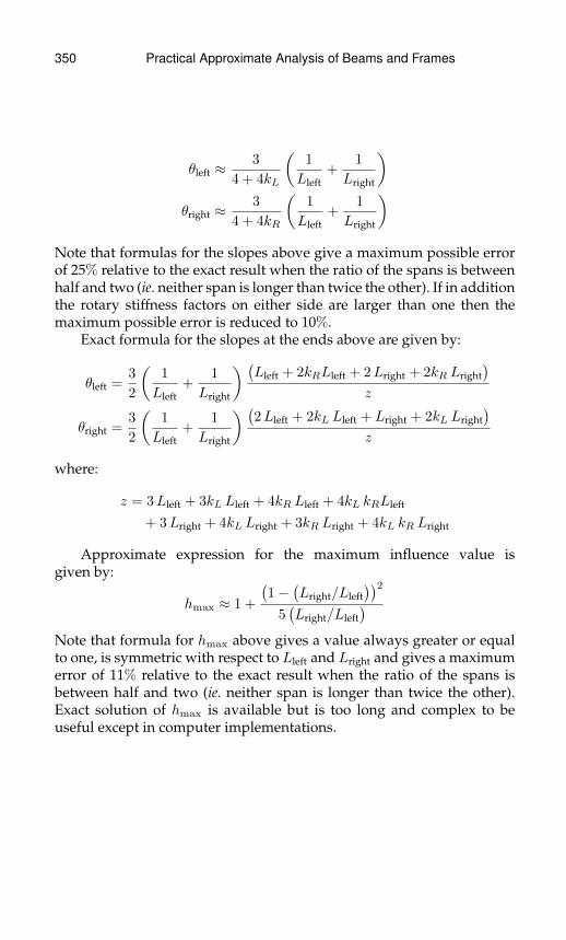
350 Practical Approximate Analysis of Beams and Frames
θleft ≈3
4 + 4kL
(1
Lleft+
1
Lright
)θright ≈
3
4 + 4kR
(1
Lleft+
1
Lright
)Note that formulas for the slopes above give a maximum possible errorof 25% relative to the exact result when the ratio of the spans is betweenhalf and two (ie. neither span is longer than twice the other). If in additionthe rotary stiffness factors on either side are larger than one then themaximum possible error is reduced to 10%.
Exact formula for the slopes at the ends above are given by:
θleft =3
2
(1
Lleft+
1
Lright
) (Lleft + 2kRLleft + 2Lright + 2kR Lright
)z
θright =3
2
(1
Lleft+
1
Lright
) (2Lleft + 2kL Lleft + Lright + 2kL Lright
)z
where:
z = 3Lleft + 3kL Lleft + 4kR Lleft + 4kL kRLleft
+ 3Lright + 4kL Lright + 3kR Lright + 4kL kR Lright
Approximate expression for the maximum influence value isgiven by:
hmax ≈ 1 +
(1−
(Lright/Lleft
))25(Lright/Lleft
)Note that formula for hmax above gives a value always greater or equalto one, is symmetric with respect to Lleft and Lright and gives a maximumerror of 11% relative to the exact result when the ratio of the spans isbetween half and two (ie. neither span is longer than twice the other).Exact solution of hmax is available but is too long and complex to beuseful except in computer implementations.
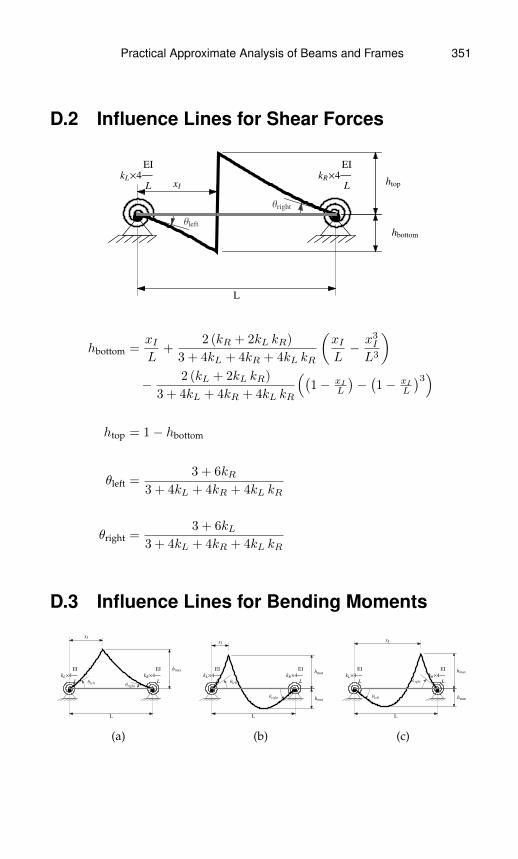
Practical Approximate Analysis of Beams and Frames 351
D.2 Influence Lines for Shear Forces
Θleft
Θright
htop
hbottom
kL´4
EI
L
kR´4
EI
L
L
xI
hbottom =xIL
+2 (kR + 2kL kR)
3 + 4kL + 4kR + 4kL kR
(xIL− x3
I
L3
)− 2 (kL + 2kL kR)
3 + 4kL + 4kR + 4kL kR
((1− xI
L
)−(1− xI
L
)3)
htop = 1− hbottom
θleft =3 + 6kR
3 + 4kL + 4kR + 4kL kR
θright =3 + 6kL
3 + 4kL + 4kR + 4kL kR
D.3 Influence Lines for Bending Moments
ΘleftΘright
hmax
kL´4
EI
L
kR´4
EI
L
L
xI
Θleft
Θright
hmax
hmin
kL´4
EI
L
kR´4
EI
L
L
xI
Θleft
Θright
hmax
hmin
kL´4
EI
L
kR´4
EI
L
L
xI
(a) (b) (c)
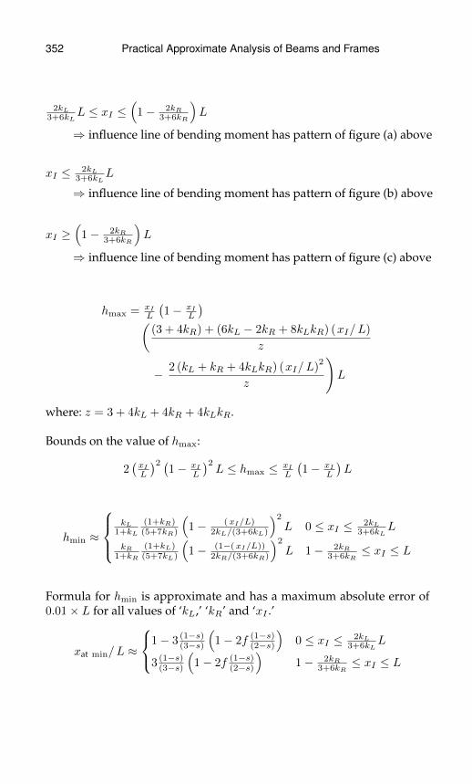
352 Practical Approximate Analysis of Beams and Frames
2kL3+6kL
L ≤ xI ≤(
1− 2kR3+6kR
)L
⇒ influence line of bending moment has pattern of figure (a) above
xI ≤ 2kL3+6kL
L
⇒ influence line of bending moment has pattern of figure (b) above
xI ≥(
1− 2kR3+6kR
)L
⇒ influence line of bending moment has pattern of figure (c) above
hmax = xI
L
(1− xI
L
)((3 + 4kR) + (6kL − 2kR + 8kLkR) (xI/L)
z
− 2 (kL + kR + 4kLkR) (xI/L)2
z
)L
where: z = 3 + 4kL + 4kR + 4kLkR.
Bounds on the value of hmax:
2(xI
L
)2 (1− xI
L
)2L ≤ hmax ≤ xI
L
(1− xI
L
)L
hmin ≈
kL
1+kL
(1+kR)(5+7kR)
(1− (xI/L)
2kL/(3+6kL)
)2
L 0 ≤ xI ≤ 2kL3+6kL
L
kR1+kR
(1+kL)(5+7kL)
(1− (1−(xI/L))
2kR/(3+6kR)
)2
L 1− 2kR3+6kR
≤ xI ≤ L
Formula for hmin is approximate and has a maximum absolute error of0.01× L for all values of ‘kL,’ ‘kR’ and ‘xI .’
xat min/L ≈
1− 3 (1−s)(3−s)
(1− 2f (1−s)
(2−s)
)0 ≤ xI ≤ 2kL
3+6kLL
3 (1−s)(3−s)
(1− 2f (1−s)
(2−s)
)1− 2kR
3+6kR≤ xI ≤ L
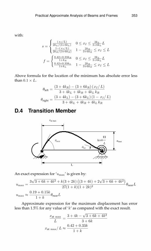
Practical Approximate Analysis of Beams and Frames 353
with:
s =
(xI/L)
2kL/(3+6kL) 0 ≤ xI ≤ 2kL3+6kL
L1−(xI/L)
2kR/(3+6kR) 1− 2kR3+6kR
≤ xI ≤ L
f =
{0.42+0.33kR
1+kR0 ≤ xI ≤ 2kL
3+6kLL
0.42+0.33kL1+kL
1− 2kR3+6kR
≤ xI ≤ L
Above formula for the location of the minimum has absolute error lessthan 0.1× L.
θleft =(3 + 4kR)− (3 + 6kR) (xI/L)
3 + 4kL + 4kR + 4kL kR
θright =(3 + 4kL)− (3 + 6kL) (1− xI/L)
3 + 4kL + 4kR + 4kL kR
D.4 Transition Member
Θnear
Θfar
umax
xat max
k´4
EI
L
L
An exact expression for ‘umax’ is given by:
umax =3√
3 + 6k + 4k2 + k(3 + 2k)((3 + 4k) + 2
√3 + 6k + 4k2
)27(1 + k)(1 + 2k)2
θnearL
umax ≈0.19 + 0.15k
1 + kθnearL
Approximate expression for the maximum displacement has errorless than 1.5% for any value of ‘k’ as compared with the exact result.
xat max
L=
3 + 4k −√
3 + 6k + 4k2
3 + 6k
xat max/L ≈ 0.42 + 0.33k
1 + k
354 Practical Approximate Analysis of Beams and Frames
Approximate expression of the location has error less than 1% forany value of ‘k’ compared to the exact result.
Note: The above results are available in a different appendix but selectedresults pertaining to influence lines are reproduced above.
Index
A
Aluminum, maximumstrain, 207
Approximate influence lines,indeterminatebeams, 231–312
bending momentsinfluence lines, 258–64isolated member, influence
line, influence lines,283–84
shear force, influencelines, 256
sketching influence lines,influence lines,306–11
reciprocity theorem, 233shear forces, influence lines,
249–54statically determinate beams,
exact influence lines,238–66
bending moments, 255–66shear forces, 246–55statically determinate
beams, sketchinginfluence line, 238
vertical force reactions,238–46
statically indeterminatestructures, 266–312
bending moments inisolated member,influence line,278–86
bending momentssketching influencelines, 304–12
influence line, 266–67shear forces, sketching
influence lines,297–305
shear forces in isolatedmember, influenceline, 274–78
transition member for alltypes, influence line,286–97
vertical reaction forces inisolated member,influence line,268–74
transition member for alltypes, influence line
transition member,influence linessketch, 287
vertical force reactions,influence lines,289–91, 294–96
vertical force reactions,vertical reactionforce, influence lines,239–44
vertical reaction forces inisolated member,influence line,vertical reaction,influence lines,268, 271
355
356 Index
B
Beams-end-moments, inflectionpoints, 313–22
moment-end-loaded beam,313–14
point force, 317–22one end fixed, 321–22one end hinged, 320–21symmetric spring
resistance,318–19
uniformly distributed load,315–17
one end fixed, 317one end hinged, 316symmetric spring
resistance, 316Bending moments, 255–66
bending moment, influencelines, 258–64
continuous beam, 17, 20influence lines, 258–64,
283–84, 306–11,351–53
isolated member, influenceline, 278–86
bending moment, influencelines, 283–84
shear force, influencelines, 256
sketching influence lines,304–12
bending moments,influence lines,306–11
C
Cantilever, 323single floor portal frame,
103–13apparent stiffness factor,
110, 112
far end resisting moment,apparent stiffnessfactors, 110
portal frame, 105, 110role of beam resisting
moment, 105rotary stiffness, column
modeled, beamattached, 107
rotationally flexiblestructure, cantileverattached to, 104
single story sidesway,113
special cases-displacements,346–47
Carry-over-factor for moments,11–13
Central point force, end conditionsof beam, 42
Class of building, analysis, 209Column-shear stiffness,
end-moments,inflection points,323–30
cantilever, 323multi-story building, column
for, 329–30multi-story building-first
floor, column for,326–27
multi-story building-top floor,column for, 328–29
single story building, columnfor, 324–25
Comparable magnitude, separatedby one member, 71
Comparison between exact,approximate shearstiffness, 141, 145,147, 149
Concrete, maximumstrain, 207
Index 357
Continuous beamapplied unit clockwise
moment, 19moment applied at only one
node, 16–20bending moment,
continuous beam, 17,20
continuous beam, appliedunit clockwisemoment, 19
inflection point locations,deformed shape, 19
isolated members ofcontinuous beam,17–18
straight line extensions,each node, 17
unit clockwise moment,continuous beam, 17
Contour plot, inflection point vs.end stiffness, 25, 50
Convention for positive, negativecurvatures, 2
D
Decomposition, deformed shapes,39–40
Decomposition passive structure,6
Deconstructing structure intoactive member,passive parts, 5
Decrease in deformation,continuous beam, 14
Deformed shapes, 39–40, 92decomposition, 67uniformly loaded beam,
symmetric supports,33
Displacements, 183–229inertia moment, 189–200maximum deflection
location, 184–85, 187value, 184–85, 187–88
maximum verticaldisplacements,183–88
maximum deflections,calculating, 184
moment of inertia, moment ofinertia, relative tohorizontal axis,194–95
relative vertical displacementsvs. strain, 200–208
aluminum, maximumstrain, 207
concrete, maximum strain,207
displacement correctionfactor, uniform load,203–4
steel, maximum strain, 207structural material strain,
207thermoplastics, maximum
strain, 207wood, maximum strain, 207
rotary stiffness factors, slopemeasurements,222–29
side displacements, framessubject to side loads,208–22
class of building, analysis,209
slenderness ratio, axialforce variation, 212
Distributed load, decompositionof structure, 71–72
E
Effective bending stiffness, 9End moments, 121–22
columns, 141, 146–47, 149

358 Index
End stiffness factors, loaded beam,function, 95
Exact deformed shapes, 75, 77Exact stiffness, determining, 8Exact vs. approximate location,
inflection points,moments obtainedfrom, 30
External moment, common node,90
F
Far end resisting moment,apparent stiffnessfactors, 110
Far end to near end rotation, ratio,13–14
First iteration calculations, 141,143, 147–48
Fixed-spring supports, 38, 66Frame building type, lumped
mass shear stiffnessvs. exact shearstiffness, 150, 152
Free body diagram, 142
H
Hinge-spring supports, 36, 65Hinged beam with applied
moment at one end,rotary spring, 12
Horizontal loadmultiple floor frames subject
to, 139–50column cases, sketching
deformation, 163comparison between exact,
approximate shearstiffness, 141, 145,147, 149
end moments, columns,141, 146–47, 149
first iteration calculations,141, 143, 147–48
free body diagram, 142multi-story sidesway, 141,
147second iteration calculation,
147–48second iteration
calculations, 141, 145shear forces, columns, 141,
146–47, 149side-loaded frames
only top floor loaded,deformation, 160,162
uniform distribution ofloads per floor,deformation, 161
sketching, 158–69slope tangent to chord,
164–65stiffness factors, 141–42, 147
single floor frames subject to,113–22
end moments in beamscalculating, 119–20portals, beams,
continuous beam, nosidesway, 120
end moments in columnscalculating, 118–19shear forces, end
moments, columns,113, 119
rotary stiffness factorestimation, 114–16
stiffness factor ofconnected beams,naming convention,115
second portal frame, 120–22end moments, 121–22shear forces, 121–22
Index 359
shear stiffness, shearforce, end moments,121
single story sidesway, 121stiffness factors, 121
shear stiffness, shear force,116–18
end moments, 113, 118free body diagram, 117
I
Inertia moment, 189–200Inflection point
beams-end-moments, 313–22moment-end-loaded beam,
313–14point force, 317–22uniformly distributed load,
315–17exact vs. approximate
location, 56moment diagram, 54point force
one end fixed, 321–22one end hinged, 320–21symmetric spring
resistance, 318–19uniformly distributed load
one end fixed, 317one end hinged, 316symmetric spring
resistance, 316Inflection point as rotary spring
stiffness increases, 15Inflection point location, 14–16
carry-over-moment, 13deformed shape, 19between exact, approximate,
26, 51Influence lines, 266–67, 349–54
bending moments, 351–53shear force, 351
transition member, 353–54vertical force reactions, 349–50
Internal hingemoment applied at one end,
resisting at other,96–93
deformed shapes, 92external moment, common
node, 90internal hinge part of
passive structure, 87moment diagrams, 92–93normalized near end
stiffness factor,contours, 87, 89
optimizing location, 90–91as passive structure,
continuous beam, 89part of passive structure, 87passive structures, deformed
shapes, 99, 101point force loaded beam
beam with, 97–102internal hinge, passive
structures, deformedshapes, 99, 101
moment diagrams, 99–101uniform load, 95
beam with, 93–96end stiffness factors, loaded
beam, function, 95moment diagrams, 96uniformly loaded beam,
deformed shapes for,passive structures, 96
Isolated members of continuousbeam, 17–18
L
Lack of sidesway, 1–102analysis method, 20–22beams, 83–84
360 Index
centerline through middleunloaded member, 78
continuous beam, momentapplied at only onenode, 16–20
bending moment,continuous beam,17, 20
continuous beam, appliedunit clockwisemoment, 19
inflection point locations,deformed shape, 19
isolated members ofcontinuous beam,17–18
straight line extensions,each node, 17
unit clockwise moment,continuous beam, 17
decomposition of structure,67, 69
end conditions, 45exact vs. approximate
location, 56fixed-spring supports, 66internal hinge
moment applied at one end,resisting at other,96–93
uniform load, 95lack of structure sidesway,
analysis method,20–22
moment applied at one end,resisting at other
beam with, 11–16carry-over-moment, 13decrease in deformation,
continuous beam, 14hinged beam with applied
moment at one end,rotary spring, 12
inflection point location,13
inflection points as rotaryspring stiffnessincreases, 15
location at which deflectionmaximum, 16
location of inflection point,14–16
magnitude of maximumdeflection, 16
moment at near end, beamrotary spring, 12
ratio of far end bendingmoment to near endbending moment,11–13
ratio of far end to near endrotation, 13–14
rotary stiffness at nearend, 13
moment diagram, 54multiple loads, 70–78
comparable magnitude,separated by onemember, 71
distributed load,decomposition ofstructure, 71–72
exact deformed shapes,75, 77
multiple adjacent loads, 76point force load,
decomposition ofstructure, deformedshapes, 71, 73
sum of separate singleloads, 72
passive members incontinuous beams,frames, 4–11
decomposing passivestructure, 6
Index 361
deconstructing structureinto active member,passive parts, 5
determining exact stiffnessin special cases, 8
effective bending stiffness, 9rotational stiffness,
estimating, 8point force loaded beam,
42–66central point force, end
conditions of beam, 42centrally applied, end
conditions, 43contour plot, inflection
point vs. endstiffnesses, 50
deformed shapes,decomposition, 67
example, 66–69fixed-spring supports, 66hinge-spring supports, 65inflection point location
between exact,approximate, 51
maximum displacement, 54maximum positive bending
moments, inflectionpoints, 57
moment diagrams, 49,67, 69
non-centrally applied, 47non-symmetric supports, 64normalized distance,
contours, 59passive structures, 48point force, right-end
stiffness factor, 60symmetric spring
resistance, 61symmetric supports,
uniformly loadedbeam, 63
sketching, 1–4convention for positive,
negative curvatures,2
loading of simple slenderbeam, 2
sketching deformed shapeof beam, 4
sketching deformed shapedof beam, 4
steps in sketching deformedshape of beam, 3
symmetry loaded, 77two/more internal hinges
beam with, 78–86bending moment
diagrams, 86internal hinges, passive
structure, 79internal hinges loaded by
uniform load,83, 85
zero bending stiffness,two-hinged beam, 80
uniformly load beam, 22–38contour plot, inflection
point vs. endstiffness, 25
decomposition, deformedshapes, 39–40
decomposition of structurewith, 39, 41
deformed shape, uniformlyloaded beam,symmetric supports,33
deformed structure shape,39–40
end conditions, 22–23exact vs. approximate
location, inflectionpoints, momentsobtained from, 30
362 Index
example, 39–42fixed-spring supports, 38hinge-spring supports, 36inflection point location
between exact,approximate, 26
location of inflection points,moment diagram, 29
maximum displacement,location, magnitude,28
maximum momentlocation, 31
moment diagrams, 24non-symmetric supports, 34one end fixed, 37one end hinged, 35passive structures, 23slopes, relative slopes,
uniformly loadedbeam, 27
symmetric springresistance, 32
symmetric supports,uniformly loadedbeam, 33
Lines of influence, 349–54Loading of simple slender beam, 2Location of inflection points,
moment diagram, 29Lower fixed support, single floor
columns,deformation, 123
Lower hinged support, single floorcolumns,deformation, 124
Lumped mass model forbuildings, 150–58
frame building type, lumpedmass shear stiffnessvs. exact shearstiffness, 150
frame building type analyzed,
lumped mass shearstiffness, exact shearstiffness, 152
lumped-mass system, framedbuilding, 151
normalized shear stiffness,mean maximumover minimumratios, 150, 153, 157
M
Maximum deflectioncalculating, 184location, 184–85, 187magnitude, 16value, 184–85, 187–88
Maximum vertical displacements,183–88
maximum deflectionlocation, 184–85, 187value, 184–85, 187–88
maximum deflections,calculating, 184
Moment applied at one end,resisting at other
beam with, 11–16carry-over-moment, 13decrease in deformation,
continuous beam, 14hinged beam, applied
moment at one end,rotary spring, 12
inflection point location,13–16
inflection points as rotaryspring stiffnessincreases, 15
location at which deflectionmaximum, 16
magnitude of maximumdeflection, 16
moment at near end, beamrotary spring, 12
Index 363
ratio, far end, near endrotation, 13–14
ratio of far-end bendingmoment to near endbending moment,11–13
rotary stiffness, near end, 13Moment diagrams, 49, 67, 69,
92–93, 96, 99–101decomposition of structure,
67, 69decomposition of structure
with, 39, 41fixed-spring supports, 66
Moment-end-loaded beam, 313–14Moment of inertia, relative to
horizontal axis, 194–95Multi-story building
column for, 329–30first floor, column for, 326–27top floor, column for, 328–29
Multi-story sidesway, 141, 147Multiple adjacent loads, 76Multiple loads, 70–78
comparable magnitude,separated by onemember, 71
distributed load,decomposition ofstructure, 71–72
exact deformed shapes, 75, 77multiple adjacent loads, 76point force load,
decomposition ofstructure, deformedshapes, 71, 73
sum of separate single loads, 72symmetric structure, loading
centerline through middleunloaded member, 78
symmetry loaded, 77Mutual shear stiffnesses, columns,
132
N
No sidesway, 1–102analysis method, 20–22approximate analysis,
1–102continuous beam, moment
applied at only onenode, 16–20
bending moment,continuous beam,17, 20
continuous beam,applied unitclockwise moment,19
inflection point locations,deformed shape, 19
isolated members ofcontinuous beam,17–18
straight line extensions,each node, 17
unit clockwise moment,continuous beam, 17
internal hingemoment applied at one
end, resisting atother, 96–93
point force loaded beambeam with, 97–102internal hinge, passive
structures, deformedshapes, 99, 101
moment diagrams,99–101
uniform load, 95beam with, 93–96end stiffness factors,
loaded beam,function, 95
moment diagrams, 96uniformly loaded
364 Index
beam, deformedshapes for, passivestructures, 96
internal hinge momentapplied at one end,resisting at other
deformed shapes, 92external moment,
common node, 90internal hinge part of
passive structure, 87moment diagrams, 92–93normalized near end
stiffness factor,contours, 87, 89
optimizing location,90–91
as passive structure,continuous beam, 89
lack of structure sidesway,analysis method,20–22
moment applied at one end,resisting at other
beam with, 11–16carry-over-moment, 13decrease in deformation,
continuous beam, 14hinged beam with
applied moment atone end, rotaryspring, 12
inflection point, 14–16inflection point location,
13inflection points as rotary
spring stiffnessincreases, 15
location at whichdeflectionmaximum, 16
magnitude of maximumdeflection, 16
moment at near end,beam rotary spring,12
ratio of far end, near endrotation, 13–14
ratio of far-end bendingmoment to near endbending moment,11–13
rotary stiffness, nearend, 13
multiple loads, 70–78comparable magnitude,
separated by onemember, 71
distributed load,decomposition ofstructure, 71–72
exact deformed shapes,75, 77
multiple adjacent loads,76
point force load,decomposition ofstructure, deformedshapes, 71, 73
sum of separate singleloads, 72
symmetric structure,loading
centerline throughmiddle unloadedmember, 78
symmetry loaded,77
passive members incontinuous beams,frames, 4–11
decomposing passivestructure, 6
deconstructing structureinto active member,passive parts, 5
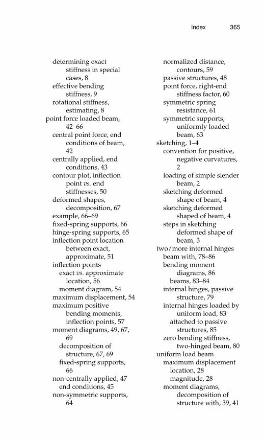
Index 365
determining exactstiffness in specialcases, 8
effective bendingstiffness, 9
rotational stiffness,estimating, 8
point force loaded beam,42–66
central point force, endconditions of beam,42
centrally applied, endconditions, 43
contour plot, inflectionpoint vs. endstiffnesses, 50
deformed shapes,decomposition, 67
example, 66–69fixed-spring supports, 66hinge-spring supports, 65inflection point location
between exact,approximate, 51
inflection pointsexact vs. approximate
location, 56moment diagram, 54
maximum displacement, 54maximum positive
bending moments,inflection points, 57
moment diagrams, 49, 67,69
decomposition ofstructure, 67, 69
fixed-spring supports,66
non-centrally applied, 47end conditions, 45
non-symmetric supports,64
normalized distance,contours, 59
passive structures, 48point force, right-end
stiffness factor, 60symmetric spring
resistance, 61symmetric supports,
uniformly loadedbeam, 63
sketching, 1–4convention for positive,
negative curvatures,2
loading of simple slenderbeam, 2
sketching deformedshape of beam, 4
sketching deformedshaped of beam, 4
steps in sketchingdeformed shape ofbeam, 3
two/more internal hingesbeam with, 78–86bending moment
diagrams, 86beams, 83–84
internal hinges, passivestructure, 79
internal hinges loaded byuniform load, 83
attached to passivestructures, 85
zero bending stiffness,two-hinged beam, 80
uniform load beammaximum displacement
location, 28magnitude, 28
moment diagrams,decomposition ofstructure with, 39, 41
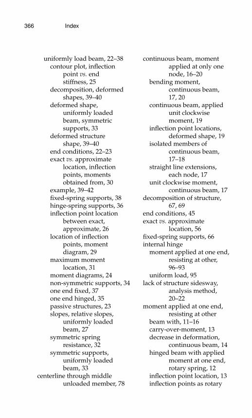
366 Index
uniformly load beam, 22–38contour plot, inflection
point vs. endstiffness, 25
decomposition, deformedshapes, 39–40
deformed shape,uniformly loadedbeam, symmetricsupports, 33
deformed structureshape, 39–40
end conditions, 22–23exact vs. approximate
location, inflectionpoints, momentsobtained from, 30
example, 39–42fixed-spring supports, 38hinge-spring supports, 36inflection point location
between exact,approximate, 26
location of inflectionpoints, momentdiagram, 29
maximum momentlocation, 31
moment diagrams, 24non-symmetric supports, 34one end fixed, 37one end hinged, 35passive structures, 23slopes, relative slopes,
uniformly loadedbeam, 27
symmetric springresistance, 32
symmetric supports,uniformly loadedbeam, 33
centerline through middleunloaded member, 78
continuous beam, momentapplied at only onenode, 16–20
bending moment,continuous beam,17, 20
continuous beam, appliedunit clockwisemoment, 19
inflection point locations,deformed shape, 19
isolated members ofcontinuous beam,17–18
straight line extensions,each node, 17
unit clockwise moment,continuous beam, 17
decomposition of structure,67, 69
end conditions, 45exact vs. approximate
location, 56fixed-spring supports, 66internal hinge
moment applied at one end,resisting at other,96–93
uniform load, 95lack of structure sidesway,
analysis method,20–22
moment applied at one end,resisting at other
beam with, 11–16carry-over-moment, 13decrease in deformation,
continuous beam, 14hinged beam with applied
moment at one end,rotary spring, 12
inflection point location, 13inflection points as rotary
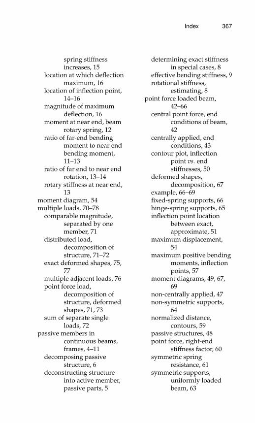
Index 367
spring stiffnessincreases, 15
location at which deflectionmaximum, 16
location of inflection point,14–16
magnitude of maximumdeflection, 16
moment at near end, beamrotary spring, 12
ratio of far-end bendingmoment to near endbending moment,11–13
ratio of far end to near endrotation, 13–14
rotary stiffness at near end,13
moment diagram, 54multiple loads, 70–78
comparable magnitude,separated by onemember, 71
distributed load,decomposition ofstructure, 71–72
exact deformed shapes, 75,77
multiple adjacent loads, 76point force load,
decomposition ofstructure, deformedshapes, 71, 73
sum of separate singleloads, 72
passive members incontinuous beams,frames, 4–11
decomposing passivestructure, 6
deconstructing structureinto active member,passive parts, 5
determining exact stiffnessin special cases, 8
effective bending stiffness, 9rotational stiffness,
estimating, 8point force loaded beam,
42–66central point force, end
conditions of beam,42
centrally applied, endconditions, 43
contour plot, inflectionpoint vs. endstiffnesses, 50
deformed shapes,decomposition, 67
example, 66–69fixed-spring supports, 66hinge-spring supports, 65inflection point location
between exact,approximate, 51
maximum displacement,54
maximum positive bendingmoments, inflectionpoints, 57
moment diagrams, 49, 67,69
non-centrally applied, 47non-symmetric supports,
64normalized distance,
contours, 59passive structures, 48point force, right-end
stiffness factor, 60symmetric spring
resistance, 61symmetric supports,
uniformly loadedbeam, 63

368 Index
sketching, 1–4convention for positive,
negative curvatures, 2loading of simple slender
beam, 2sketching deformed shape
of beam, 4sketching deformed shaped
of beam, 4steps in sketching deformed
shape of beam, 3symmetry loaded, 77two/more internal hinges
beam with, 78–86bending moment diagrams,
86internal hinges, passive
structure, 79internal hinges loaded by
uniform load, 83, 85zero bending stiffness,
two-hinged beam, 80uniformly load beam, 22–38
contour plot, inflectionpoint vs. endstiffness, 25
decomposition, deformedshapes, 39–40
decomposition of structurewith, 39, 41
deformed shape, uniformlyloaded beam,symmetric supports,33
deformed structure shape,39–40
end conditions, 22–23exact vs. approximate
location, inflectionpoints, momentsobtained from, 30
example, 39–42fixed-spring supports, 38
hinge-spring supports, 36inflection point location
between exact,approximate, 26
location of inflection points,moment diagram, 29
maximum displacement,location, magnitude,28
maximum momentlocation, 31
moment diagrams, 24non-symmetric supports, 34one end fixed, 37one end hinged, 35passive structures, 23slopes, relative slopes,
uniformly loadedbeam, 27
symmetric springresistance, 32
symmetric supports,uniformly loadedbeam, 33
Non-centrally applied, 47end conditions, 45
Non-symmetric supports, 34, 64Normalized distance, contours, 59Normalized near end stiffness
factor, contours, 87,89
Normalized shear stiffness, meanmaximum overminimum ratios, 150,153, 157
O
Optimizing location, 90–91
P
Passive members in continuousbeams, frames, 4–11

Index 369
decomposing passivestructure, 6
deconstructing structure intoactive member,passive parts, 5
determining exact stiffness inspecial cases, 8
effective bending stiffness, 9rotational stiffness,
estimating, 8Passive structures, 48Point force, 317–22
one end fixed, 321–22one end hinged, 320–21right-end stiffness factor, 60symmetric spring resistance,
318–19Point force-centrally loaded-mid
displacements,338–39
Point force load, 42–66central point force, end
conditions ofbeam, 42
centrally applied, endconditions, 43
contour plot, inflection pointvs. end stiffnesses, 50
decomposition of structure,deformed shapes,71, 73
deformed shapes,decomposition, 67
example, 66–69fixed-spring supports, 66hinge-spring supports, 65inflection point location
between exact,approximate, 51
inflection pointsexact vs. approximate
location, 56moment diagram, 54
maximum displacement, 54maximum positive bending
moments, inflectionpoints, 57
moment diagrams, 49, 67, 69decomposition of structure,
67, 69fixed-spring supports, 66
non-centrally applied, 47end conditions, 45
non-symmetric supports, 64normalized distance,
contours, 59passive structures, 48point force, right-end stiffness
factor, 60symmetric spring resistance,
61symmetric supports,
uniformly loadedbeam, 63
Point force-loaded anywhere-middisplacements,340–42
Point moment-loadedanywhere-middisplacements,343–45
Portal frame, 105, 110Portals, beams, continuous beam,
no sidesway, 120
R
Reciprocity theorem, 233Relative vertical displacements vs.
strain, 200–208aluminum, maximum strain,
207concrete, maximum strain,
207displacement correction
factor, uniform load,203–4
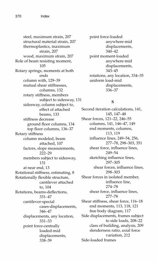
370 Index
steel, maximum strain, 207structural material strain, 207thermoplastics, maximum
strain, 207wood, maximum strain, 207
Role of beam resisting moment,105
Rotary springs, moments at bothends
column with, 129–39mutual shear stiffnesses,
columns, 132rotary stiffness, members
subject to sidesway, 131sidesway, column subject to,
effect of attachedbeams, 133
stiffness decreaseground floor columns, 134top floor columns, 136–37
Rotary stiffnesscolumn modeled, beam
attached, 107factors, slope measurements,
222–29members subject to sidesway,
131at near end, 13
Rotational stiffness, estimating, 8Rotationally flexible structure,
cantilever attachedto, 104
Rotations, beams-deflections,331–47
cantilever-specialcases-displacements,346–47
displacements, any location,331–33
point force-centrallyloaded-middisplacements,338–39
point force-loadedanywhere-middisplacements,340–42
point moment-loadedanywhere-middisplacements,343–45
rotations, any location, 334–35uniform load-mid
displacements,336–37
S
Second iteration calculations, 141,145, 147–48
Shear forces, 121–22, 246–55columns, 141, 146–47, 149end moments, columns,
113, 119influence lines, 249–54, 256,
277–78, 298–303, 351shear force, influence lines,
249–54sketching influence lines,
297–305shear forces, influence lines,
298–303Shear forces in isolated member,
influence line,274–78
shear force, influence lines,277–78
Shear stiffness, shear force, 116–18end moments, 113, 118, 121free body diagram, 117
Side displacements, frames subjectto side loads, 208–22
class of building, analysis, 209slenderness ratio, axial force
variation, 212Side-loaded frames
Index 371
only top floor loaded,deformation, 160,162
uniform distribution of loadsper floor,deformation, 161
Sideswaycolumn subject to, effect of
attached beams, 133end moments in beams
calculating, 119–20portals, beams, continuous
beam, no sidesway,120
end moments in columnscalculating, 118–19shear forces, end moments,
columns, 113, 119frame cantilever, single floor
portal frameapparent stiffness factor,
110, 112far end resisting moment,
apparent stiffnessfactors, 110
portal frame, 105, 110role of beam resisting
moment, 105rotary stiffness, column
modeled, beamattached, 107
rotationally flexiblestructure, cantileverattached to, 104
single story sidesway,113
frame horizontal load, singlefloor frames subject to
rotary stiffness factorestimation, 114–16
second portal frame, 120–22shear stiffness, shear force,
116–18
frame horizontal loads,multiple floor framessubject to
column cases, sketchingdeformation, 163
comparison between exact,approximate shearstiffness, 141, 145,147, 149
end moments, columns,141, 146–47, 149
first iteration calculations,141, 143, 147–48
free body diagram, 142multi-story sidesway, 141,
147second iteration calculation,
147–48second iteration
calculations, 141, 145shear forces, columns, 141,
146–47, 149sketching, 158–69slope tangent to chord,
164–65stiffness factors, 141–42, 147
frame lumped mass model forbuildings
frame building type,lumped mass shearstiffness vs. exactshear stiffness, 150
frame building typeanalyzed, lumpedmass shear stiffness,exact shear stiffness,152
lumped-mass system,framed building, 151
normalized shear stiffness,mean maximumover minimumratios, 150, 153, 157
372 Index
frame rotary springs,moments at bothends
column with, 129–39mutual shear stiffnesses,
columns, 132rotary stiffness, members
subject to sidesway,131
sidesway, column subjectto, effect of attachedbeams, 133
frame single floor portalframes
lower fixed support, singlefloor columns,deformation, 123
lower hinged support,single floor columns,deformation, 124
sketching, 122–29sketching deformed shape,
steps, 126–27frame vertical loads, applied
couples, sideswaydue to
frame subject to verticalload, sidesway, 170
side frame moves, freebody diagrams, 170
sidesway to left or to right,conditionsdetermining, 171,173–74, 176
single floor regular portalframe, variablenumber of bays, 177
frames with, 103–81cantilever, single floor
portal frame, 103–13horizontal load, single floor
frames subject to,113–22
horizontal loads, multiplefloor frames subjectto, 139–50
lumped mass model forbuildings, 150–58
vertical loads, appliedcouples, sideswaydue to, 169–81
moment applied at one end,resisting at other
deformed shapes, 92external moment, common
node, 90internal hinge part of
passive structure, 87moment diagrams, 92–93normalized near end
stiffness factor,contours, 87, 89
optimizing location, 90–91as passive structure,
continuous beam, 89point force loaded beam
beam with, 97–102internal hinge, passive
structures, deformedshapes, 99, 101
moment diagrams, 99–101rotary stiffness factor
estimation, stiffnessfactor of connectedbeams, namingconvention, 115
second portal frameend moments, 121–22shear forces, 121–22shear stiffness, shear force,
end moments, 121single story sidesway, 121stiffness factors, 121
shear stiffness, shear forceend moments, 113, 118free body diagram, 117

Index 373
side-loaded framesonly top floor loaded,
deformation, 160,162
uniform distribution ofloads per floor,deformation, 161
stiffness decreaseground floor columns, 134top floor columns, 136–37
uniform loadbeam with, 93–96end stiffness factors, loaded
beam, function, 95moment diagrams, 96uniformly loaded beam,
deformed shapes for,passive structures, 96
Sidesway lack, 1–102analysis method, 20–22beams, 83–84centerline through middle
unloaded member,78
continuous beam, momentapplied at only onenode, 16–20
bending moment,continuous beam, 17,20
continuous beam, appliedunit clockwisemoment, 19
inflection point locations,deformed shape, 19
isolated members ofcontinuous beam, 17–18
straight line extensions,each node, 17
unit clockwise moment,continuous beam, 17
decomposition of structure,67, 69
end conditions, 45exact vs. approximate
location, 56fixed-spring supports, 66internal hinge
moment applied at one end,resisting at other,96–93
uniform load, 95lack of structure sidesway,
analysis method,20–22
moment applied at one end,resisting at other
beam with, 11–16carry-over-moment, 13decrease in deformation,
continuous beam, 14hinged beam with applied
moment at one end,rotary spring, 12
inflection point location, 13inflection points as rotary
spring stiffnessincreases, 15
location at which deflectionmaximum, 16
location of inflection point,14–16
magnitude of maximumdeflection, 16
moment at near end, beamrotary spring, 12
ratio of far-end bendingmoment to near endbending moment,11–13
ratio of far end to near endrotation, 13–14
rotary stiffness at near end,13
moment diagram, 54multiple loads, 70–78
374 Index
comparable magnitude,separated by onemember, 71
distributed load,decomposition ofstructure, 71–72
exact deformed shapes,75, 77
multiple adjacent loads, 76point force load,
decomposition ofstructure, deformedshapes, 71, 73
sum of separate singleloads, 72
passive members incontinuous beams,frames, 4–11
decomposing passivestructure, 6
deconstructing structureinto active member,passive parts, 5
determining exact stiffnessin special cases, 8
effective bending stiffness, 9rotational stiffness,
estimating, 8point force loaded beam,
42–66central point force, end
conditions of beam,42
centrally applied, endconditions, 43
contour plot, inflectionpoint vs. endstiffnesses, 50
deformed shapes,decomposition, 67
example, 66–69fixed-spring supports, 66hinge-spring supports, 65
inflection point locationbetween exact,approximate, 51
maximum displacement, 54maximum positive bending
moments, inflectionpoints, 57
moment diagrams, 49, 67, 69non-centrally applied, 47non-symmetric supports, 64normalized distance,
contours, 59passive structures, 48point force, right-end
stiffness factor, 60symmetric spring
resistance, 61symmetric supports,
uniformly loadedbeam, 63
sketching, 1–4convention for positive,
negative curvatures,2
loading of simple slenderbeam, 2
sketching deformed shapeof beam, 4
sketching deformed shapedof beam, 4
steps in sketching deformedshape of beam, 3
symmetry loaded, 77two/more internal hinges
beam with, 78–86bending moment diagrams,
86internal hinges, passive
structure, 79internal hinges loaded by
uniform load, 83, 85zero bending stiffness,
two-hinged beam, 80

Index 375
uniformly load beam,22–38
contour plot, inflectionpoint vs. endstiffness, 25
decomposition, deformedshapes, 39–40
decomposition of structurewith, 39, 41
deformed shape, uniformlyloaded beam,symmetric supports,33
deformed structure shape,39–40
end conditions, 22–23exact vs. approximate
location, inflectionpoints, momentsobtained from, 30
example, 39–42fixed-spring supports, 38hinge-spring supports, 36inflection point location
between exact,approximate, 26
location of inflection points,moment diagram, 29
maximum displacement,location, magnitude,28
maximum momentlocation, 31
moment diagrams, 24non-symmetric supports, 34one end fixed, 37one end hinged, 35passive structures, 23slopes, relative slopes,
uniformly loadedbeam, 27
symmetric springresistance, 32
symmetric supports,uniformly loadedbeam, 33
Single floor portal framecantilever, 103–13
apparent stiffness factor,110, 112
far end resisting moment,apparent stiffnessfactors, 110
portal frame, 105, 110role of beam resisting
moment, 105rotary stiffness, column
modeled, beamattached, 107
rotationally flexiblestructure, cantileverattached to, 104
single story sidesway, 113lower fixed support, single
floor columns,deformation, 123
lower hinged support, singlefloor columns,deformation, 124
sketching, 122–29sketching deformed shape,
steps, 126–27Single story column, 324–25Single story sidesway,
113, 121Sketching, 1–4, 122–29, 158–69
convention for positive,negativecurvatures, 2
deformed shapebeam, 3–4steps, 126–27
loading of simple slenderbeam, 2
Slenderness ratio, axial forcevariation, 212

376 Index
Sloperelative slopes, uniformly
loaded beam, 27tangent to chord, 164–65
Statically determinate beamsexact influence lines,
238–66bending moments,
255–66shear forces, 246–55statically determinate
beams, sketchinginfluence line, 238
vertical force reactions,238–46
sketching influence line, 238Statically indeterminate structures,
266–312bending moments, sketching
influence lines,304–12
bending moments,influence lines,306–11
bending moments in isolatedmember, influenceline, 278–86
bending moment, influencelines, 283–84
influence line, 266–67shear forces, sketching
influence lines,297–305
shear forces, influence lines,298–303
shear forces in isolatedmember, influenceline, 274–78
shear force, influence lines,277–78
transition member for alltypes, influence line,286–97
transition member,influence linessketch, 287
vertical force reactions,influence lines,289–91, 294–96
vertical reaction forces inisolated member,influence line,268–74
vertical reaction, influencelines, 268, 271
Steel, maximum strain, 207Steps in sketching deformed shape
of beam, 3Stiffness decrease
ground floor columns, 134top floor columns, 136–37
Stiffness factors, 121, 141–42, 147apparent, 110, 112connected beams, naming
convention, 115Straight line extensions, each
node, 17Strain, vs. relative vertical
displacements,200–208
aluminum, maximum strain,207
concrete, maximum strain, 207displacement correction
factor, uniform load,203–4
steel, maximum strain, 207structural material strain, 207thermoplastics, maximum
strain, 207wood, maximum strain, 207
Symmetric spring resistance, 32, 61Symmetric structure, loading
centerline through middleunloaded member, 78
symmetry loaded, 77
Index 377
Symmetric supports, uniformlyloaded beam, 33, 63
T
Thermoplastics, maximum strain,207
Transition member, influencelines, 353–54
sketch, 287Transition member for all types,
influence line,286–97
transition member, influencelines sketch, 287
vertical force reactions,influence lines,289–91, 294–96
Two/more internal hingesbeam with, 78–86bending moment diagrams,
86beams, 83–84
internal hinges loaded byuniform load, 83
attached to passivestructures, 85
internal hinges passivestructure, 79
zero bending stiffness,two-hinged beam, 80
U
Uniform load-mid displacements,336–37
Uniformly distributed load,315–17
one end fixed, 317one end hinged, 316symmetric spring resistance,
316Uniformly loaded beam, 22–38
contour plot, inflection pointvs. end stiffness, 25
decomposition, deformedshapes, 39–40
deformed shape, uniformlyloaded beam,symmetric supports,33
deformed shapes for, passivestructures, 96
deformed structure shape,39–40
end conditions, 22–23exact vs. approximate
location, inflectionpoints, momentsobtained from, 30
example, 39–42fixed-spring supports, 38hinge-spring supports, 36inflection point location
between exact,approximate, 26
location of inflection points,moment diagram, 29
maximum displacementlocation, 28
magnitude, 28magnitude, 28
maximum moment location,31
moment diagrams, 24decomposition of structure
with, 39, 41non-symmetric supports, 34one end fixed, 37one end hinged, 35passive structures, 23slopes, relative slopes,
uniformly loadedbeam, 27
symmetric spring resistance, 32symmetric supports,
uniformly loadedbeam, 33
378 Index
Unit clockwise moment,continuous beam, 17
V
Vertical displacements, 183–88maximum deflection
location, 184–85, 187value, 184–85, 187–88
maximum deflections,calculating, 184
Vertical displacements vs. strain,200–208
aluminum, maximum strain,207
concrete, maximum strain,207
displacement correctionfactor, uniform load,203–4
steel, maximum strain, 207structural material strain, 207thermoplastics, maximum
strain, 207wood, maximum strain, 207
Vertical force reactions, 238–46influence lines, 289–91,
294–96, 349–50vertical reaction force,
influence lines,239–44
Vertical loads, applied couples,sidesway due to,169–81
frame subject to vertical load,sidesway, 170
side frame moves, free bodydiagrams, 170
sidesway to left or to right,conditions determining,171, 173–74, 176
single floor regular portalframe, variablenumber of bays, 177
Vertical reaction, influence lines,268, 271
Vertical reaction forcesinfluence lines, 239–44isolated member, influence
line, 268–74vertical reaction, influence
lines, 268, 271
W
Wood, maximum strain, 207
Z
Zero bending stiffness,two-hinged beam
two/more internal hinges,lack of sidesway, 80