practical sketching algorithms for low-rank matrix...

SIAM J. MATRIX ANAL. APPL. c© 2017 Society for Industrial and Applied MathematicsVol. 38, No. 4, pp. 1454–1485

PRACTICAL SKETCHING ALGORITHMS FOR LOW-RANKMATRIX APPROXIMATION∗

JOEL A. TROPP† , ALP YURTSEVER‡ , MADELEINE UDELL§ , AND VOLKAN CEVHER‡

Abstract. This paper describes a suite of algorithms for constructing low-rank approximationsof an input matrix from a random linear image, or sketch, of the matrix. These methods can preservestructural properties of the input matrix, such as positive-semidefiniteness, and they can produceapproximations with a user-specified rank. The algorithms are simple, accurate, numerically stable,and provably correct. Moreover, each method is accompanied by an informative error bound thatallows users to select parameters a priori to achieve a given approximation quality. These claims aresupported by numerical experiments with real and synthetic data.

Key words. dimension reduction, matrix approximation, numerical linear algebra, randomizedalgorithm, single-pass algorithm, sketching, streaming algorithm, subspace embedding

AMS subject classifications. Primary, 65F30; Secondary, 68W20

DOI. 10.1137/17M1111590

1. Motivation. This paper presents a framework for computing structured low-rank approximations of a matrix from a sketch, which is a random low-dimensionallinear image of the matrix. Our goal is to develop simple, practical algorithms thatcan serve as reliable modules in other applications. The methods apply for the realfield (F = R) and for the complex field (F = C).

1.1. Low-rank matrix approximation. Suppose that A ∈ Fm×n is an arbi-trary matrix. Let r be a target rank parameter where r minm,n. The com-putational problem is to produce a low-rank approximation A of A whose error iscomparable to a best rank-r approximation:

(1.1) ‖A− A‖F ≈ minrank(B)≤r

‖A−B‖F.

The notation ‖ · ‖F refers to the Frobenius norm. We explicitly allow the rank of Ato exceed r because we can obtain more accurate approximations of this form, andthe precise rank of A is unimportant in many applications. There has been extensiveresearch on randomized algorithms for (1.1); see Halko, Martinsson, and Tropp [19].

1.2. Sketching. Here is the twist. Imagine that our interactions with the matrixA are severely constrained in the following way. We construct a linear map L :Fm×n → Fd that does not depend on the matrix A. Our only mechanism for collecting

∗Received by the editors January 17, 2017; accepted for publication (in revised form) by August18, 2017; published electronically December 6, 2017.

http://www.siam.org/journals/simax/38-4/M111159.htmlFunding: The work of the first and third authors was supported in part by ONR award N00014-

11-1002 and the Gordon & Betty Moore Foundation. The work of the third author was also supportedin part by DARPA award FA8750-17-2-0101. The work of the second and fourth authors was sup-ported in part by the European Commission under the ERC Future Proof grant and grants SNF200021-146750, and SNF CRSII2-147633.†Computing and Mathematical Sciences, California Institute of Technology, Pasadena, CA 91125-

5000 ([email protected]).‡Ecole Polytechnique Federal de Lausanne, Lausanne 1015, Switzerland ([email protected],

[email protected]).§Cornell University, Ithaca, NY 14853 ([email protected]).

1454

http://www.siam.org/journals/simax/38-4/M111159.html

mailto:[email protected]




SKETCHING ALGORITHMS FOR MATRIX APPROXIMATION 1455

data S about A is to apply the linear map L :

(1.2) S := L (A) ∈ Fd.

We refer to S as a sketch of the matrix, and L is called a sketching map. The numberd is called the dimension or size of the sketch.

The challenge is to make the sketch as small as possible while collecting enoughinformation to approximate the matrix accurately. In particular, we want the sketchdimension d to be much smaller than the total dimension mn of the matrix A. Asa consequence, the sketching map L has a substantial null space. Therefore, it isnatural to draw the sketching map at random so that we are likely to extract usefulinformation from any fixed input matrix.

1.3. Why sketch? There are a number of situations where the sketching model(1.2) is a natural mechanism for acquiring data about an input matrix.

First, imagine that A is a huge matrix that can only be stored outside of corememory. The cost of data transfer may be substantial enough that we can only affordto read the matrix into core memory once [19, sect. 5.5]. We can build a sketchas we scan through the matrix. Other types of algorithms for this problem appearin [15, 16].

Second, there are applications where the columns of the matrix A are revealedone at a time, and we must be able to compute an approximation at any instant. Oneapproach is to maintain a sketch that is updated when a new column arrives. Othertypes of algorithms for this problem appear in [4, 21].

Third, we may encounter a setting where the matrix A is presented as a sum ofordered updates:

(1.3) A = H1 + H2 + H3 + H4 + · · · .

We must discard each innovation Hi after it is processed [9, 34]. In this case, therandom linear sketch (1.2) is more or less the only way to maintain a representationof A through an arbitrary sequence of updates [23]. Our research was motivated bya variant [36] of the model (1.3); see subsection 3.8.

1.4. Overview of algorithms. Let us summarize our basic approach to sketch-ing and low-rank approximation of a matrix. Fix a target rank r and an input matrixA ∈ Fm×n. Select sketch size parameters k and `. Draw and fix independent stan-dard normal matrices Ω ∈ Fn×k and Ψ ∈ F`×m; see Definition 2.1. We realize therandomized linear sketch (1.2) via left and right matrix multiplication:

(1.4) Y := AΩ and W := ΨA.

We can store the random matrices and the sketch using (k + `)(m+ n) scalars. Thearithmetic cost of forming the sketch is Θ((k+ `)mn) floating-point operations (flops)for a general matrix A.

Given the random matrices (Ω,Ψ) and the sketch (Y ,W ), we compute an ap-proximation A in three steps:

1. Form an orthogonal–triangular factorization Y =: QR, where Q ∈ Fm×k.2. Solve a least-squares problem to obtain X := (ΨQ)†W ∈ Fk×n.3. Construct the rank-k approximation A := QX.

The total cost of this computation is Θ(kl(m + n)) flops. See subsection 4.2 for theintuition behind this approach.

1456 J. A. TROPP, A. YURTSEVER, M. UDELL, AND V. CEVHER

Now, suppose that we set the sketch size parameters k = 2r + 1 and ` = 4r + 2.For this choice, Theorem 4.3 yields the error bound

E ‖A− A‖F ≤ 2 · minrank(B)≤r

‖A−B‖F.

In other words, we typically obtain an approximation with rank ≈ 2r whose errorlies within twice the optimal rank-r error! Moreover, the total storage cost is about6r(m + n), which is comparable to the number of degrees of freedom in an m × nmatrix with rank r, so the sketch size cannot be reduced substantially.

1.5. Our contributions. This paper presents a systematic treatment of sketch-ing algorithms for low-rank approximation of a matrix. All of the methods rely onthe simple sketch (1.4) of the input matrix (subsection 3.5). The main algorithm usesthis sketch to compute a high-quality low-rank approximation A of the input matrix(Algorithm 4). We prove that this method automatically takes advantage of spectraldecay in the input matrix (Theorem 4.3); this result is new.

We also explain how to compute approximations with additional structure—such as symmetry, positive semidefiniteness, or fixed rank—by projecting the initiallow-rank approximation onto the family of structured matrices (sections 5 and 6).This approach ensures that the structured approximations also exploit spectral decay(Fact 5.1 and Proposition 6.1). In the sketching context, this idea is new.

Each algorithm is accompanied by an informative error bound that provides agood description of its actual behavior. As a consequence, we can offer the firstconcrete guidance on algorithm parameters for various types of input matrices (sub-section 4.5), and we can implement the methods with confidence. We also includepseudocode and an accounting of computational costs.

The paper includes a collection of numerical experiments (section 7). This workdemonstrates that the recommended algorithms can significantly outperform alter-native methods, especially when the input matrix has spectral decay. The empiricalwork also confirms our guidance on parameter choices.

Our technical report [32] contains some more error bounds for the reconstructionalgorithms. It also documents additional numerical experiments.

1.6. Limitations. The algorithms in this paper are not designed for all low-rank matrix approximation problems. They are specifically intended for environmentswhere we can only make a single pass over the input matrix or where the data matrixis presented as a stream of linear updates. When it is possible to make multiple passesover the input matrix, we recommend the low-rank approximation algorithms docu-mented in [19]. Multipass methods are significantly more accurate because they drivethe error of the low-rank approximation down to the optimal low-rank approximationerror exponentially fast in the number of passes.

1.7. Overview of related work. Randomized algorithms for matrix approx-imation date back to research [30, 17] in theoretical computer science (TCS) in thelate 1990s. Starting around 2004, this work inspired numerical analysts to developpractical algorithms for matrix approximation and related problems [26]. See the pa-per [19, sect. 2] for a comprehensive historical discussion. The surveys [25, 34] providemore details about the development of these ideas within the TCS literature.

1.7.1. Sketching algorithms for matrix approximation. To the best of ourknowledge, the first sketching algorithm for low-rank matrix approximation appearsin Woolfe et al. [35, sect. 5.2]. Their primary motivation was to compute a low-rank


matrix approximation faster than any classical algorithm, rather than to work underthe constraints of a sketching model. A variant of their approach is outlined in [19,sect. 5.5].

Clarkson and Woodruff [9] explicitly frame the question of how to perform numer-ical linear algebra tasks under the sketching model (1.2). Among other things, theydevelop algorithms and lower bounds for low-rank matrix approximation. Some ofthe methods that we recommend are algebraically—but not numerically—equivalentto formulas [9, Thms. 4.7 and 4.8] that they propose. Their work focuses on obtaininga priori error bounds. In contrast, we also aim to help users implement the methods,choose parameters, and obtain good empirical performance in practice. Additionaldetails appear throughout our presentation.

There are many subsequent theoretical papers on sketching algorithms for low-rank matrix approximation, including [34, 12, 6]. This line of research exploits avariety of tricks to obtain algorithms that, theoretically, attain better asymptotic up-per bounds on computational resource usage. Subsection 7.3 contains a representativeselection of these methods and their guarantees.

1.7.2. Note added in press. When we wrote this paper, the literature did notcontain sketching methods tailored for symmetric or positive-semidefinite (psd) matrixapproximation. A theoretical paper [8] on algorithms for low-rank approximation ofa sparse psd matrix was released after our work appeared.

1.7.3. Error bounds. Almost all previous papers in this area have centered onthe following problem. Let A ∈ Fm×n be an input matrix, let r be a target rank, andlet ε > 0 be an error tolerance. Given a randomized linear sketch (1.2) of the inputmatrix, produce a rank-r approximation Aeps that satisfies

(1.5) ‖A− Aeps‖2F ≤ (1 + ε) · minrank(B)≤r

‖A−B‖2F with high probability.

To achieve (1.5) for a general input, the sketch must have dimension Ω(r(m + n)/ε)[9, Thm. 4.10]. Furthermore, the analogous error bound for the spectral norm cannotbe achieved for all input matrices under the sketching model [34, Chap. 6.2]. Never-theless, Gu [18, Thm. 3.4] has observed that (1.5) implies a weak error bound in thespectral norm.

Li et al. [22, App.] caution that the guarantee (1.5) is often vacuous. For example,we frequently encounter matrices for which the Frobenius-norm error of an optimalrank-r approximation is larger than the Frobenius norm of the approximation itself.In other settings, it may be necessary to compute an approximation with very highaccuracy. Either way, ε must be tiny before the bound (1.5) sufficiently constrainsthe approximation error. For a general input matrix, to achieve a small value of ε,the sketch size must be exorbitant. We tackle this issue by providing alternative errorestimates (e.g., Theorem 4.3) that yield big improvements for most examples.

1.7.4. Questions.... Our aim is to address questions that arise when one at-tempts to use sketching algorithms in practice. For instance, how do we implementthese methods? Are they numerically stable? How should algorithm parameters de-pend on the input matrix? What is the right way to preserve structural properties?Which methods produce the best approximations in practice? How small an ap-proximation error can we actually achieve? Does existing theoretical analysis predictperformance? Can we obtain error bounds that are more illuminating than (1.5)?These questions have often been neglected in the literature.


Our empirical study (section 7) highlights the importance of this inquiry. Surpris-ingly, numerical experiments reveal that the pursuit of theoretical metrics has beencounterproductive. More recent algorithms often perform worse in practice, eventhough—in principle—they offer better performance guarantees.

2. Background. In this section, we collect notation and conventions, as well assome background on random matrices.

2.1. Notation and conventions. We write F for the scalar field, which is eitherR or C. The letter I signifies the identity matrix; its dimensions are determined bycontext. The asterisk ∗ refers to the (conjugate) transpose operation on vectors andmatrices. The dagger † is the Moore–Penrose pseudoinverse. The symbol ‖·‖F denotesthe Frobenius norm.

The expression “M has rank r” and its variants mean that the rank of M does notexceed r. The symbol JMKr represents an optimal rank-r approximation of M withrespect to the Frobenius norm; this approximation need not be unique [20, sect. 6].

It is valuable to introduce notation for the error incurred by a best rank-r ap-proximation in the Frobenius norm. For each natural number j, we define the jth tailenergy

(2.1) τ2j (A) := min

rank(B)<j‖A−B‖2F =

∑i≥j

σ2i (A).

We have written σi(A) for the ith largest singular value of A. The equality followsfrom the Eckart–Young theorem; for example, see [20, sect. 6].

The symbol E denotes expectation with respect to all random variables. Fora given random variable Z, we write EZ to denote expectation with respect to therandomness in Z only. Nonlinear functions bind before the expectation.

In the description of algorithms in the text, we primarily use standard mathe-matical notation. In the pseudocode, we rely on some MATLAB R2017a functions inan effort to make the presentation more concise.

We use the computer science interpretation of Θ(·) to refer to the class of functionswhose growth is bounded above and below up to a constant.

2.2. Standard normal matrices. Let us define an ensemble of random matri-ces that plays a central role in this work.

Definition 2.1 (standard normal matrix). A matrix G ∈ Rm×n has the realstandard normal distribution if the entries form an independent family of standardnormal random variables (i.e., Gaussian with mean zero and variance one).

A matrix G ∈ Cm×n has the complex standard normal distribution if it has theform G = G1+iG2, where G1 and G2 are independent, real standard normal matrices.

Standard normal matrices are also known as Gaussian matrices.

We introduce numbers α and β that reflect the field over which the random matrixis defined:

(2.2) α := α(F) :=

1, F = R,0, F = C,

and β := β(F) :=

1, F = R,2, F = C.

This notation allows us to treat the real and complex cases simultaneously. Thenumber β is a standard parameter in random matrix theory.


Finally, we introduce notation to help make our theorem statements more suc-cinct:

(2.3) f(s, t) :=s

t− s− αfor integers that satisfy t > s+ α > α.

Observe that the function f(s, ·) is decreasing, with range (0, s].

3. Sketching the input matrix. First, we discuss how to collect enough dataabout an input matrix to compute a low-rank approximation. We summarize thematrix by multiplying it on the right and the left by random test matrices. Thedimension and distribution of these random test matrices together determine thepotential accuracy of the approximation.

3.1. The input matrix. Let A ∈ Fm×n be a matrix that we wish to approxi-mate. Our algorithms work regardless of the relative dimensions of A, but there maysometimes be small benefits if we apply them to A∗ instead.

3.2. The target rank. Let r be a target rank parameter with 1 ≤ r ≤ minm,n.We aim to construct a low-rank approximation of A whose error is close to the op-timal rank-r error. We explicitly allow approximations with rank somewhat largerthan r because they may be significantly more accurate.

Under the sketching model (1.2), the practitioner must use prior knowledge aboutthe input matrix A to determine a target rank r that will result in satisfactory errorguarantees. This decision is outside the scope of our work.

3.3. Parameters for the sketch. The sketch consists of two parts: a summaryof the range of A and a summary of the co-range. The parameter k controls the sizeof the range sketch, and the parameter ` controls the size of the co-range sketch. Theyshould satisfy the conditions

(3.1) r ≤ k ≤ ` and k ≤ n and ` ≤ m.

We often choose k ≈ r and ` ≈ k. See (4.6) and subsection 4.5 below.The parameters k and ` do not play symmetrical roles. We need ` ≥ k to ensure

that a certain `× k matrix has full column rank. Larger values of both k and ` resultin better approximations at the cost of more storage and arithmetic. These trade-offsare quantified in what follows.

3.4. The test matrices. To form the sketch of the input matrix, we draw andfix two (random) test matrices:

(3.2) Ω ∈ Fn×k and Ψ ∈ F`×m.

This paper contains a detailed analysis of the case where the test matrices are sta-tistically independent and follow the standard normal distribution. Subsection 3.9describes other potential distributions for the test matrices. We always state whenwe are making distributional assumptions on the test matrices.

3.5. The sketch. The sketch of A ∈ Fm×n consists of two matrices:

(3.3) Y := AΩ ∈ Fm×k and W := ΨA ∈ F`×n.

The matrix Y collects information about the action of A, while the matrix W collectsinformation about the action of A∗. Both parts are necessary.


Algorithm 1 Sketch for Low-Rank Approximation. Implements (3.2) and (3.3).

Require: Input matrix A ∈ Fm×n; sketch size parameters k ≤ `Ensure: Constructs test matrices Ω ∈ Fn×k and Ψ ∈ F`×m, range sketch Y = AΩ ∈

Fm×k, and co-range sketch W = ΨA ∈ F`×n as private variables

1 private: Ω,Ψ,Y ,W . Internal variables for Sketch object. Accessible to all Sketch methods

2 function Sketch(A; k, `) . Constructor3 if F = R then4 Ω← randn(n, k)5 Ψ← randn(`,m)6 if F = C then7 Ω← randn(n, k) + i randn(n, k)8 Ψ← randn(`,m) + i randn(`,m)9 Ω← orth(Ω) . (optional) Improve numerical stability

10 Ψ∗ ← orth(Ψ∗) . (optional) Improve numerical stability11 Y ← AΩ12 W ← ΨA

Remark 3.1 (prior work). The matrix sketching algorithms that appear in [35,sect. 5.2], [9, Thm. 4.9], [19, sect. 5.5], and [34, Thm. 4.3] all involve a sketch of theform (3.3). In contrast, the most recent approaches ([6, sect. 6.1.2] and [33, sect. 3])use more complicated sketches; see subsection 7.3.2.

3.6. The sketch as an abstract data type. We present the sketch as anabstract data type using ideas from object-oriented programming. Sketch is anobject that contains information about a specific matrix A. The test matrices (Ω,Ψ)and the sketch matrices (Y ,W ) are private variables that are only accessible to theSketch methods. A user interacts with the Sketch object by initializing it with aspecific matrix and by applying linear updates. The user can query the Sketch objectto obtain an approximation of the matrix A with specific properties. The individualalgorithms described in this paper are all methods that belong to the Sketch object.

3.7. Initializing the sketch and its costs. See Algorithm 1 for pseudocodethat implements the sketching procedure (3.2) and (3.3) with either standard normaltest matrices (default) or random orthonormal test matrices (optional steps). Notethat the orthogonalization step requires additional arithmetic and communication.

The storage cost for the sketch (Y ,W ) is mk+ `n floating-point numbers in thefield F. The storage cost for two standard normal test matrices is nk + `m floating-point numbers in F. Some other types of test matrices (Ω,Ψ) have lower storagecosts, but the sketch (Y ,W ) remains the same size.

For standard normal test matrices, the arithmetic cost of forming the sketch (3.3)is Θ((k + `)mn) flops when A is dense. If A is sparse, the cost is proportional tothe number nnz(A) of nonzero entries: Θ((k + `) nnz(A)) flops. Other types of testmatrices sometimes yield lower arithmetic costs.


Algorithm 2 Linear Update to Sketch. Implements (3.4).

Require: Update matrix H ∈ Fm×n; scalars θ, η ∈ FEnsure: Modifies sketch (Y ,W ) to reflect linear update A← θA + ηH

1 function Sketch.LinearUpdate(H; θ, η)2 Y ← θY + ηHΩ . Linear update to range sketch3 W ← θW + ηΨH . Linear update to co-range sketch

3.8. Processing linear updates. The sketching model (3.3) supports a linearupdate that is more general than (1.3). Suppose the input matrix A is modified as

A← θA + ηH, where θ, η ∈ F.

Then we update the sketch (3.3) via the rule

(3.4) Y ← θY + ηHΩ and W ← θW + ηΨH.

The precise cost of the computation depends on the structure of H. See Algorithm 2for the pseudocode. This type of update is crucial for certain applications [36].

3.9. Choosing the distribution of the test matrices. Our analysis is spe-cialized to the case where the test matrices Ω and Ψ are standard normal so that wecan obtain highly informative error bounds.

But there are potential benefits from implementing the sketch using test matricesdrawn from another distribution. The choice of distribution leads to some trade-offs in the range of permissible parameters; the costs of randomness, arithmetic, andcommunication to generate the test matrices; the storage costs for the test matricesand the sketch; the arithmetic costs for sketching and updates; the numerical stabilityof matrix approximation algorithms; and the quality of a priori error bounds.

Let us list some of the contending distributions along with background references.We have ranked these in decreasing order of reliability.

• Orthonormal. The optional steps in Algorithm 1 generate matrices Ω andΨ∗ with orthonormal columns that span uniformly random subspaces of di-mension k and `. When k and ` are very large, these matrices result in smallererrors and better numerical stability than Gaussians [14, 19].

• Gaussian. Following [26, 19], this paper focuses on test matrices with thestandard normal distribution. Benefits include excellent practical perfor-mance and accurate a priori error bounds.

• Rademacher. These test matrices have independent Rademacher1 entries.Their behavior is similar to Gaussian test matrices, but there are minor im-provements in the cost of storage and arithmetic, as well as the amount ofrandomness required. For example, see [9].

• Subsampled randomized Fourier transform (SRFT). These test ma-trices take the form

(3.5) Ω = D1F1P1 and Ψ = P2F∗2 D2,

1A Rademacher random variable takes the values ±1 with equal probability.


where D1 ∈ Fn×n and D2 ∈ Fm×m are diagonal matrices with independentRademacher entries; F1 ∈ Fn×n and F2 ∈ Fm×m are discrete cosine transform(F = R) or discrete Fourier transform (F = C) matrices; and P1 ∈ Fn×k andP2 ∈ F`×m are restrictions onto k and ` coordinates, chosen uniformly atrandom. These matrices work well in practice, they require a modest amountof storage, and they support fast arithmetic. See [1, 35, 2, 19, 31, 5, 13].

• Ultrasparse Rademacher. Let s be a sparsity parameter. In each rowof Ω and column of Ψ, we place independent Rademacher random variablesin s uniformly random locations; the remaining entries of the test matricesare zero. These matrices help control storage, arithmetic, and randomnesscosts. On the other hand, they are somewhat less reliable. For more details,see [10, 28, 27, 29, 34, 3, 11].

Except for ultrasparse Rademacher matrices, these distributions often behave quitelike a Gaussian distribution in practice [19, sect. 7.4]. An exhaustive comparison ofdistributions for the test matrices is outside the scope of this paper; see [24].

4. Low-rank approximation from the sketch. Suppose that we have ac-quired a sketch (Y ,W ) of the input matrix A, as in (3.2) and (3.3). This sectionpresents the most basic algorithm for computing a low-rank approximation of A fromthe data in the sketch. This simple approach is similar to earlier proposals; see [35,sect. 5.2], [9, Thm. 4.7], [19, sect. 5.5], and [34, Thm. 4.3, display 1].

We have obtained the first accurate error bound for this method. Our resultshows how the spectrum of the input matrix affects the approximation quality. Thisanalysis allows us to make parameter recommendations for specific input matrices.

In section 5, we explain how to refine this algorithm to obtain approximationswith additional structure. In section 6, we describe modifications of the proceduresthat produce approximations with fixed rank and additional structure. Throughout,we maintain the notation of section 3.

4.1. The main algorithm. Our goal is to produce a low-rank approximationof the input matrix A using only the knowledge of the test matrices (Ω,Ψ) and thesketch (Y ,W ). Here is the basic method.

The first step in the procedure is to compute an orthobasis for the range of Y bymeans of an orthogonal–triangular factorization:

(4.1) Y =: QR, where Q ∈ Fm×k.

The matrix Q has orthonormal columns; we discard the triangular matrix R. Thesecond step uses the co-range sketch W to form the matrix

(4.2) X := (ΨQ)†W ∈ Fk×n.

The random matrix ΨQ ∈ F`×k is very well-conditioned when ` k, so we canperform this computation accurately by solving a least-squares problem. We reportthe rank-k approximation

(4.3) A := QX ∈ Fm×n, where Q ∈ Fm×k and X ∈ Fk×n.

The factors Q and X are defined in (4.1) and (4.2).

Remark 4.1 (prior work). The approximation A is algebraically, but not numer-ically, equivalent with the approximation that appears in Clarkson and Woodruff [9,Thm. 4.7]; see also [34, Thm. 4.3, display 1]. Our formulation improves upon theirsby avoiding a badly conditioned least-squares problem.


Algorithm 3 Simplest Low-Rank Approximation. Implements (4.3).

Ensure: For some q ≤ k, returns factors Q ∈ Fm×q with orthonormal columns andX ∈ Fq×n that form a rank-q approximation Aout = QX of the sketched matrix

1 function Sketch.SimpleLowRankApprox( )2 Q← orth(Y ) . Orthobasis for range of Y3 X ← (ΨQ)\W . Multiply (ΨQ)† on left side of W4 return (Q,X)

Algorithm 4 Low-Rank Approximation. Implements (4.3).

Ensure: Returns factors Q ∈ Fm×k with orthonormal columns and X ∈ Fk×n thatform a rank-k approximation Aout = QX of the sketched matrix

1 function Sketch.LowRankApprox( )2 (Q,∼)← qr(Y , 0) . Orthobasis for range of Y3 (U ,T )← qr(ΨQ, 0) . Orthogonal–triangular factorization4 X ← T †(U∗W ) . Apply inverse by back-substitution5 return (Q,X)

4.2. Intuition. To motivate the algorithm, we recall a familiar heuristic [19,sect. 1] from randomized linear algebra, which states that

(4.4) A ≈ QQ∗A.

Although we would like to form the rank-k approximation Q(Q∗A), we cannot com-pute the factor Q∗A without revisiting the input matrix A. Instead, we exploit theinformation in the co-range sketch W = ΨA. Notice that

W = Ψ(QQ∗A) + Ψ(A−QQ∗A) ≈ (ΨQ)(Q∗A).

The heuristic (4.4) justifies dropping the second term. Multiplying on the left by thepseudoinverse (ΨQ)†, we arrive at the relation

X = (ΨQ)†W ≈ Q∗A.

These considerations suggest that

A = QX ≈ QQ∗A ≈ A.

One of our contributions is to give substance to these nebulae.

Remark 4.2 (prior work). This intuition is inspired by the discussion in [19,sect. 5.5], and it allows us to obtain sharp error bounds. Our approach is quitedifferent from that of [9, Thm. 4.7] or [34, Thm. 4.3].

4.3. Algorithm and costs. Algorithms 3 and 4 give pseudocode for computingthe approximation (4.3). The first presentation uses MATLAB functions to abbreviatesome of the steps, while the second includes more implementation details. Note thatthe use of the orth command may result in an approximation with rank q for someq ≤ k, but the quality of the approximation does not change.


Let us summarize the costs of the approximation procedure (4.1)–(4.3), as imple-mented in Algorithm 4. The algorithm has working storage of O (k(m+ n)) floating-point numbers. The arithmetic cost is Θ(k`(m+n)) flops, which is dominated by thematrix–matrix multiplications. The orthogonalization step and the back-substitutionrequire Θ(k2(m+ n)) flops, which is almost as significant.

4.4. A bound for the Frobenius-norm error. We have established a veryaccurate error bound for the approximation (4.3) that is implemented in Algorithms 3and 4. This analysis is one of the key contributions of this paper.

Theorem 4.3 (low-rank approximation: Frobenius error). Assume that the sketchsize parameters satisfy ` > k+α. Draw random test matrices Ω ∈ Fn×k and Ψ ∈ F`×mindependently from the standard normal distribution. Then the rank-k approximationA obtained from formula (4.3) satisfies

(4.5)

E ‖A− A‖2F ≤ (1 + f(k, `)) · min%<k−α

(1 + f(%, k)) · τ2%+1(A)

=k

`− k − α· min%<k−α

k

k − %− α· τ2%+1(A).

The index % ranges over natural numbers. The quantities α(R) := 1 and α(C) := 0;the function f(s, t) := s/(t− s− α); and the tail energy τ2

j is defined in (2.1).

The proof of Theorem 4.3 appears below in Appendix A.3.To begin to understand Theorem 4.3, it is helpful to consider a specific parameter

choice. Let r be the target rank of the approximation, and select

(4.6) k = 2r + α and ` = 2k + α.

For these sketch size parameters, with % = r, Theorem 4.3 implies that

E ‖A− A‖2F ≤ 4 · τ2r+1(A).

In other words, for k ≈ 2r, we can construct a rank-k approximation of A thathas almost the same quality as a best rank-r approximation. This parameter choicebalances the sketch size against the quality of approximation.

But the true meaning of Theorem 4.3 lies deeper. The minimum in (4.5) revealsthat the approximation (4.3) automatically takes advantage of decay in the tail energy.This fundamental fact explains the strong empirical performance of (4.3) and otherapproximations derived from it. Our analysis is the first to identify this feature.

Remark 4.4 (prior work). The analysis in [9, Thm. 3.7] shows that A achievesa bound of the form (1.5) when the sketch size parameters scale as k = Θ(r/ε) and` = Θ(k/ε). A precise variant of the same statement follows from Theorem 4.3.

Remark 4.5 (high-probability error bound). The expectation bound presented inTheorem 4.3 also describes the typical behavior of the approximation (4.3) becauseof measure concentration effects. It is possible to develop a high-probability boundusing the methods from [19, sect. 10.3].

Remark 4.6 (spectral-norm error bound). It is also possible to develop bounds forthe spectral-norm error incurred by the approximation (4.3). These results dependon the decay of both the singular values and the tail energies. See [32, Thm. 4.2].


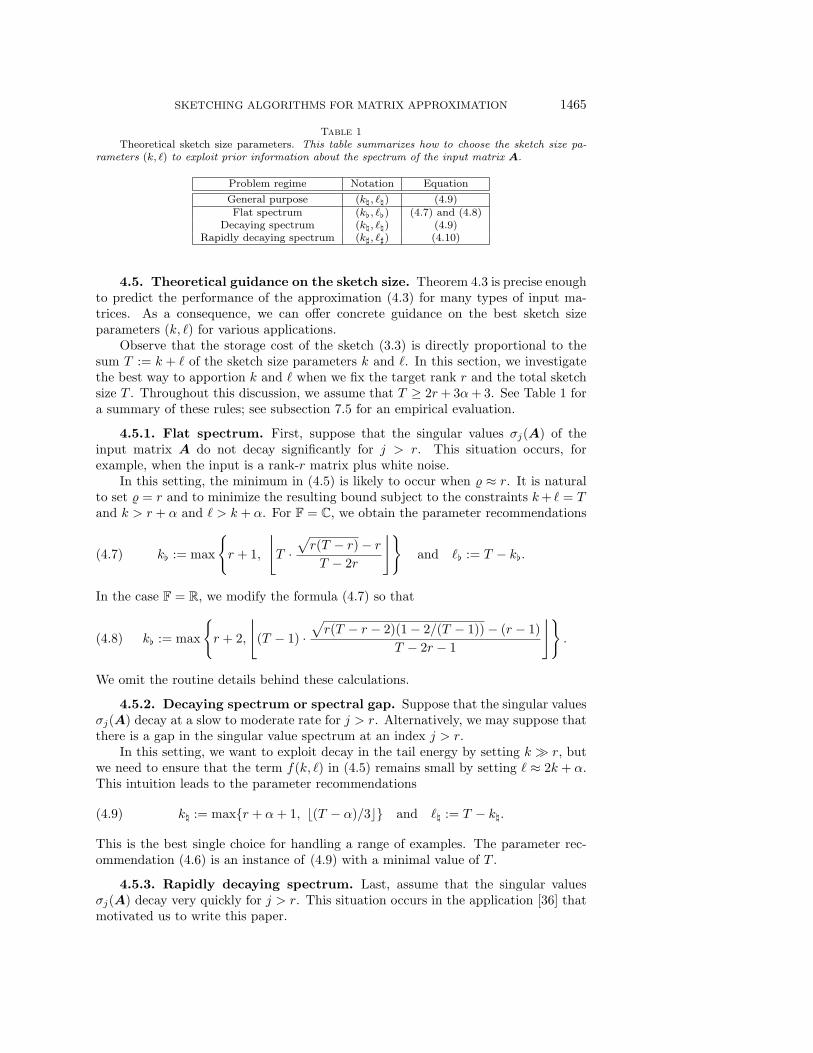
Table 1Theoretical sketch size parameters. This table summarizes how to choose the sketch size pa-

rameters (k, `) to exploit prior information about the spectrum of the input matrix A.

Problem regime Notation EquationGeneral purpose (k\, `\) (4.9)Flat spectrum (k[, `[) (4.7) and (4.8)

Decaying spectrum (k\, `\) (4.9)Rapidly decaying spectrum (k], `]) (4.10)

4.5. Theoretical guidance on the sketch size. Theorem 4.3 is precise enoughto predict the performance of the approximation (4.3) for many types of input ma-trices. As a consequence, we can offer concrete guidance on the best sketch sizeparameters (k, `) for various applications.

Observe that the storage cost of the sketch (3.3) is directly proportional to thesum T := k + ` of the sketch size parameters k and `. In this section, we investigatethe best way to apportion k and ` when we fix the target rank r and the total sketchsize T . Throughout this discussion, we assume that T ≥ 2r+ 3α+ 3. See Table 1 fora summary of these rules; see subsection 7.5 for an empirical evaluation.

4.5.1. Flat spectrum. First, suppose that the singular values σj(A) of theinput matrix A do not decay significantly for j > r. This situation occurs, forexample, when the input is a rank-r matrix plus white noise.

In this setting, the minimum in (4.5) is likely to occur when % ≈ r. It is naturalto set % = r and to minimize the resulting bound subject to the constraints k+ ` = Tand k > r + α and ` > k + α. For F = C, we obtain the parameter recommendations

(4.7) k[ := max

r + 1,

⌊T ·√r(T − r)− rT − 2r

⌋and `[ := T − k[.

In the case F = R, we modify the formula (4.7) so that

(4.8) k[ := max

r + 2,

⌊(T − 1) ·

√r(T − r − 2)(1− 2/(T − 1))− (r − 1)

T − 2r − 1

⌋.

We omit the routine details behind these calculations.

4.5.2. Decaying spectrum or spectral gap. Suppose that the singular valuesσj(A) decay at a slow to moderate rate for j > r. Alternatively, we may suppose thatthere is a gap in the singular value spectrum at an index j > r.

In this setting, we want to exploit decay in the tail energy by setting k r, butwe need to ensure that the term f(k, `) in (4.5) remains small by setting ` ≈ 2k + α.This intuition leads to the parameter recommendations

(4.9) k\ := maxr + α+ 1, b(T − α)/3c and `\ := T − k\.

This is the best single choice for handling a range of examples. The parameter rec-ommendation (4.6) is an instance of (4.9) with a minimal value of T .

4.5.3. Rapidly decaying spectrum. Last, assume that the singular valuesσj(A) decay very quickly for j > r. This situation occurs in the application [36] thatmotivated us to write this paper.


In this setting, we want to exploit decay in the tail energy fully by setting k as largeas possible; the benefit outweighs the increase in f(k, `) from choosing ` = k+ α+ 1,the minimum possible value. This intuition leads to the parameter recommendations

(4.10) k] := b(T − α− 1)/2c and `] := T − k].

Note that the choice (4.10) is unwise unless the input matrix has sharp spectral decay.

5. Low-rank approximations with convex structure. In many instances,we need to reconstruct an input matrix that has additional structure, such as sym-metry or positive-semidefiniteness. The approximation formula (4.3) from section 4produces an approximation with no special properties aside from a bound on its rank.Therefore, we may have to reform our approximation to instill additional virtues.

In this section, we consider a class of problems where the input matrix belongsto a convex set, and we seek an approximation that belongs to the same set. Toaccomplish this goal, we replace our initial approximation with the closest point inthe convex set. This procedure always improves the Frobenius-norm error.

We address two specific examples: (i) the case where the input matrix is conjugatesymmetric, and (ii) the case where the input matrix is positive-semidefinite (psd).In both situations, we must design the algorithm carefully to avoid forming largematrices.

5.1. Projection onto a convex set. Let C be a closed and convex set ofmatrices in Fm×n. Define the projector ΠC onto the set C to be the map

ΠC : Fm×n → C where ΠC(M) := arg min‖C −M‖2F : C ∈ C

.

The arg min operator returns the matrix C? ∈ C that solves the optimization problem.The solution C? is uniquely determined because the squared Frobenius norm is strictlyconvex and the constraint set C is closed and convex.

5.2. Structure via convex projection. Suppose that the input matrix A be-longs to the closed convex set C ⊂ Fm×n. Let Ain ∈ Fm×n be an initial approximationof A. We can produce a new approximation ΠC(Ain) by projecting the initial approx-imation onto the constraint set. This procedure always improves the approximationquality in Frobenius norm.

Fact 5.1 (convex structure reduces error). Let C ∈ Fm×n be a closed convex set,and suppose that A ∈ C. For any initial approximation Ain ∈ Fm×n,

(5.1) ‖A−ΠC(Ain)‖F ≤ ‖A− Ain‖F.

This result is well known in convex analysis. It follows directly from the first-order optimality conditions [7, sect. 4.2.3] for the Frobenius-norm projection of amatrix onto the set C. We omit the details.

Warning 5.2 (spectral norm). Fact 5.1 does not hold if we replace the Frobeniusnorm by the spectral norm.

5.3. Low-rank approximation with conjugate symmetry. When the inputmatrix is conjugate symmetric, it is often critical to produce a conjugate symmetricapproximation. We can do so by combining the simple approximation from section 4with the projection step outlined in subsection 5.1.


5.3.1. Conjugate symmetric projection. Define the set Hn(F) of conjugatesymmetric matrices with dimension n over the field F:

Hn := Hn(F) := C ∈ Fn×n : C = C∗.

The set Hn(F) is convex because it forms a real-linear subspace in Fn×n. In whatfollows, we omit the field F from the notation unless there is a possibility of confusion.

The projection Msym of a matrix M ∈ Fn×n onto the set Hn takes the form

(5.2) Msym := ΠHn(M) =12

(M + M∗).

For example, see [20, sect. 2].

5.3.2. Computing a conjugate symmetric approximation. Assume thatthe input matrix A ∈ Hn is conjugate symmetric. Let A := QX be an initial rank-kapproximation of A obtained from the approximation procedure (4.3). We can forma better Frobenius-norm approximation Asym by projecting A onto Hn:

(5.3) Asym := ΠHn(A) =12

(A + A∗) =12

(QX + X∗Q∗).

The second relation follows from (5.2).In most cases, it is preferable to present the approximation (5.3) in factored form.

To do so, we observe that

12

(QX + X∗Q∗) =12[Q X∗

] [0 II 0

] [Q X∗

]∗.

Concatenate Q and X∗, and compute the orthogonal–triangular factorization

(5.4)[Q X∗

]=: U

[T1 T2

], where U ∈ Fn×2k and T1 ∈ F2k×k.

Of course, we only need to orthogonalize the k columns of X∗, which permits somecomputational efficiencies. Next, introduce the matrix

(5.5) S :=12[T1 T2

] [0 II 0

] [T1 T2

]∗ =12

(T1T∗2 + T2T

∗1 ) ∈ F2k×2k.

Combine the last four displays to obtain the rank-(2k) conjugate symmetric approxi-mation

(5.6) Asym = USU∗.

From this expression, it is easy to obtain other types of factorizations, such as aneigenvalue decomposition, by further processing.

5.3.3. Algorithm, costs, and error. Algorithm 5 contains pseudocode forproducing a conjugate symmetric approximation of the form (5.6) from a sketch ofthe input matrix. One can make this algorithm slightly more efficient by takingadvantage of the fact that Q already has orthogonal columns; we omit the details.

For Algorithm 5, the total working storage is Θ(kn) and the arithmetic cost isΘ(k`n). These costs are dominated by the call to Sketch.LowRankApprox.

Combining Theorem 4.3 with Fact 5.1, we have the following bound on the error ofthe symmetric approximation (5.6), implemented in Algorithm 5. As a consequence,the parameter recommendations from subsection 4.5 are also valid here.


Algorithm 5 Low-Rank Symmetric Approximation. Implements (5.6).

Require: Matrix dimensions m = nEnsure: For q = 2k, returns factors U ∈ Fn×q with orthonormal columns and S ∈ Hq

that form a rank-q conjugate symmetric approximation Aout = USU∗ of thesketched matrix

1 function Sketch.LowRankSymApprox( )2 (Q,X)← LowRankApprox( ) . Get Ain = QX3 (U ,T )← qr([Q,X∗], 0) . Orthogonal factorization of concatenation4 T1 ← T (:, 1:k) and T2 ← T (:, (k + 1):(2k)) . Extract submatrices5 S ← (T1T

∗2 + T2T

∗1 )/2 . Symmetrize

6 return (U ,S) . Return factors

Corollary 5.3 (low-rank symmetric approximation). Assume that the input ma-trix A ∈ Hn(F) is conjugate symmetric, and assume that the sketch size parameterssatisfy ` > k+α. Draw random test matrices Ω ∈ Fn×k and Ψ ∈ F`×n independentlyfrom the standard normal distribution. Then the rank-(2k) conjugate symmetric ap-proximation Asym produced by (5.3) or (5.6) satisfies

E ‖A− Asym‖2F ≤ (1 + f(k, `)) · min%<k−α

(1 + f(%, k)) · τ2%+1(A).



5.4. Low-rank positive-semidefinite approximation. We often encounterthe problem of approximating a psd matrix. In many situations, it is important toproduce an approximation that maintains positivity. Our approach combines theapproximation (4.3) from section 4 with the projection step from subsection 5.1.

5.4.1. Positive-semidefinite projection. We introduce the set Hn+(F) of psd

matrices with dimension n over the field F:

Hn+ := Hn

+(F) :=C ∈ Hn : z∗Cz ≥ 0 for each z ∈ Fn

.

The set Hn+(F) is convex because it is an intersection of half-spaces. In what follows,

we omit the field F from the notation unless there is a possibility for confusion.Given a matrix M ∈ Fn×n, we construct its projection onto the set Hn

+ in threesteps. First, form the projection Msym := ΠHn(M) onto the conjugate symmetricmatrices, as in (5.2). Second, compute an eigenvalue decomposition Msym =: V DV ∗.Third, form D+ by zeroing out the negative entries of D. Then the projection M+of the matrix M onto Hn

+ takes the form

M+ := ΠHn+

(M) = V D+V ∗.

For example, see [20, sect. 3].

5.4.2. Computing a positive-semidefinite approximation. Assume thatthe input matrix A ∈ Hn

+ is psd. Let A := QX be an initial approximation of Aobtained from the approximation procedure (4.3). We can form a psd approximationA+ by projecting A onto the set Hn

+.


Algorithm 6 Low-Rank Positive-Semidefinite Approximation. Implements (5.7).

Require: Matrix dimensions m = nEnsure: For q = 2k, returns factors U ∈ Fn×q with orthonormal columns and non-

negative, diagonal D ∈ Hq+ that form a rank-q psd approximation Aout = UDU∗

of the sketched matrix

1 function Sketch.LowRankPSDApprox( )2 (U ,S)← LowRankSymApprox( ) . Get Ain = USU∗

3 (V ,D)← eig(S) . Form eigendecomposition4 U ← UV . Consolidate orthonormal factors5 D ← max(D, 0) . Zero out negative eigenvalues6 return (U ,D)

To do so, we repeat the computations (5.4) and (5.5) to obtain the symmetricapproximation Asym presented in (5.6). Next, form an eigenvalue decomposition ofthe matrix S given by (5.5):

S =: V DV ∗.

In view of (5.6), we obtain an eigenvalue decomposition of Asym:

Asym = (UV )D(UV )∗.

To obtain the psd approximation A+, we simply replace D by its nonnegative partD+ to arrive at the rank-(2k) psd approximation

(5.7) A+ := ΠHn+

(A) = (UV )D+(UV )∗.

This formula delivers an approximate eigenvalue decomposition of the input matrix.

5.4.3. Algorithm, costs, and error. Algorithm 6 contains pseudocode forproducing a psd approximation of the form (5.7) from a sketch of the input matrix.As in Algorithm 5, some additional efficiencies are possible

The costs of Algorithm 6 are similar with the symmetric approximation method,Algorithm 5. The working storage cost is Θ(kn), and the arithmetic cost is Θ(k`n).

Combining Theorem 4.3 and Fact 5.1, we obtain a bound on the approximationerror identical to Corollary 5.3. We omit the details.

6. Fixed-rank approximations from the sketch. The algorithms in sec-tions 4 and 5 produce high-quality approximations with rank k, but we sometimesneed to reduce the rank to match the target rank r. At the same time, we may haveto impose additional structure. This section explains how to develop algorithms thatproduce a rank-r structured approximation.

The technique is conceptually similar to the approach in section 5. We projectan initial high-quality approximation onto the set of rank-r matrices. This procedurepreserves both conjugate symmetry and the psd property. The analysis in subsec-tion 5.1 does not apply because the set of matrices with fixed rank is not convex. Wepresent a general argument to show that the cost is negligible.

6.1. A general error bound for fixed-rank approximation. If we have agood initial approximation of the input matrix, we can replace this initial approxima-tion by a fixed-rank matrix without increasing the error significantly.


Proposition 6.1 (error for fixed-rank approximation). Let A ∈ Fm×n be a inputmatrix, and let Ain ∈ Fm×n be an approximation. For any rank parameter r,

(6.1) ‖A− JAinKr‖F ≤ τr+1(A) + 2‖A− Ain‖F.

Recall that J·Kr returns a best rank-r approximation with respect to the Frobenius norm.

Proof. Calculate that

‖A− JAinKr‖F ≤ ‖A− Ain‖F + ‖Ain − JAinKr‖F≤ ‖A− Ain‖F + ‖Ain − JAKr‖F≤ 2‖A− Ain‖F + ‖A− JAKr‖F.

The first and last relations are triangle inequalities. To reach the second line, notethat JAinKr is a best rank-r approximation of Ain, while JAKr is an undistinguishedrank-r matrix. Finally, identify the tail energy (2.1).

Remark 6.2 (spectral norm). A result analogous to Proposition 6.1 also holdswith respect to the spectral norm. The proof is the same.

6.2. Fixed-rank approximation from the sketch. Suppose that we wish tocompute a rank-r approximation of the input matrix A ∈ Fm×n. First, we forman initial approximation A := QX using the procedure (4.3). Then we obtain arank-r approximation JAKr of the input matrix by replacing A with its best rank-rapproximation in the Frobenius norm:

(6.2) JAKr = JQXKr.

We can complete this operation by working directly with the factors. Indeed,suppose that X = UΣV ∗ is an SVD of X. Then QX has an SVD of the form

QX = (QU)ΣV ∗.

As such, there is also a best rank-r approximation of QX that satisfies

JQXKr = (QU)JΣKrV ∗ = QJXKr.

Therefore, the desired rank-r approximation (6.2) can also be expressed as

(6.3) JAKr = QJXKr.

The formula (6.3) is more computationally efficient than (6.2) because the factorX ∈ Fk×n is much smaller than the approximation A ∈ Fm×n.

Remark 6.3 (prior work). The approximation JAKr is algebraically, but not nu-merically, equivalent to a formula proposed by Clarkson and Woodruff [9, Thm. 4.8].As above, our formulation improves upon theirs by avoiding a badly conditionedleast-squares problem.

6.2.1. Algorithm and costs. Algorithm 7 contains pseudocode for computingthe fixed-rank approximation (6.3).

The fixed-rank approximation in Algorithm 7 has storage and arithmetic costson the same order as the simple low-rank approximation (Algorithm 3). Indeed,to compute the truncated SVD and perform the matrix–matrix multiplication, weexpend only Θ(k2n) additional flops. Thus, the total working storage is Θ(k(m+ n))numbers and the arithmetic cost is Θ(k`(m+ n)) flops.


Algorithm 7 Fixed-Rank Approximation. Implements (6.3).

Require: Target rank r ≤ kEnsure: Returns factors Q ∈ Fm×r and V ∈ Fn×r with orthonormal columns and

nonnegative diagonal Σ ∈ Fr×r that form a rank-r approximation Aout = QΣV ∗

of the sketched matrix

1 function Sketch.FixedRankApprox(r)2 (Q,X)← LowRankApprox( ) . Get Ain = QX3 (U ,Σ,V )← svds(X, r) . Form full SVD and truncate4 Q← QU . Consolidate orthonormal factors5 return (Q,Σ,V )

6.2.2. A bound for the error. We can obtain an error bound for the rank-rapproximation (6.3) by combining Theorem 4.3 and Proposition 6.1.

Corollary 6.4 (fixed-rank approximation: Frobenius-norm error). Assume thesketch size parameters satisfy k > r + α and ` > k + α. Draw random test matricesΩ ∈ Fn×k and Ψ ∈ F`×m independently from the standard normal distribution. Thenthe rank-r approximation JAKr obtained from the formula (6.3) satisfies

(6.4) E ‖A − JAKr‖F ≤ τr+1(A) + 2√

1 + f(k, `) · min%<k−α

√1 + f(%, k) · τ%+1(A).



This result indicates that the fixed-rank approximation JAKr automatically ex-ploits spectral decay in the input matrix A. Moreover, we can still rely on theparameter recommendations from subsection 4.5. Ours is the first theory to providethese benefits.

Remark 6.5 (prior work). The analysis [9, Thm. 4.8] of Clarkson and Woodruffimplies that the approximation (6.3) can achieve the bound (1.5) for any ε > 0,provided that k = Θ(r/ε2) and ` = Θ(k/ε2). It is possible to improve this scaling;see [32, Thm. 5.1].

Remark 6.6 (spectral-norm error bound). It is possible to obtain an error boundfor the rank-r approximation (6.3) with respect to the spectral norm by combining[32, Thm. 4.2] and Remark 6.2.

6.3. Fixed-rank conjugate symmetric approximation. Assume that theinput matrix A ∈ Hn is conjugate symmetric, and we wish to compute a rank-rconjugate symmetric approximation. First, form an initial approximation Asym usingthe procedure (5.6) in subsection 5.3.2. Then compute an r-truncated eigenvaluedecomposition of the matrix S defined in (5.5):

S =: V JDKrV ∗ + approximation error.

In view of the representation (5.6),

(6.5) JAsymKr = (UV )JDKr(UV )∗.

Algorithm 8 contains pseudocode for the fixed-rank approximation (6.5). The totalworking storage is Θ(kn), and the arithmetic cost is Θ(k`n).


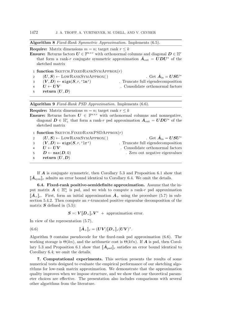
Algorithm 8 Fixed-Rank Symmetric Approximation. Implements (6.5).

Require: Matrix dimensions m = n; target rank r ≤ kEnsure: Returns factors U ∈ Fn×r with orthonormal columns and diagonal D ∈ Hr

that form a rank-r conjugate symmetric approximation Aout = UDU∗ of thesketched matrix

1 function Sketch.FixedRankSymApprox(r)2 (U ,S)← LowRankSymApprox( ) . Get Ain = USU∗

3 (V ,D)← eigs(S, r, ’lm’) . Truncate full eigendecomposition4 U ← UV . Consolidate orthonormal factors5 return (U ,D)

Algorithm 9 Fixed-Rank PSD Approximation. Implements (6.6).

Require: Matrix dimensions m = n; target rank r ≤ kEnsure: Returns factors U ∈ Fn×r with orthonormal columns and nonnegative,

diagonal D ∈ Hr+ that form a rank-r psd approximation Aout = UDU∗ of the

sketched matrix

1 function Sketch.FixedRankPSDApprox(r)2 (U ,S)← LowRankSymApprox( ) . Get Ain = USU∗

3 (V ,D)← eigs(S, r, ’lr’) . Truncate full eigendecomposition4 U ← UV . Consolidate orthonormal factors5 D ← max(D, 0) . Zero out negative eigenvalues6 return (U ,D)

If A is conjugate symmetric, then Corollary 5.3 and Proposition 6.1 show thatJAsymKr admits an error bound identical to Corollary 6.4. We omit the details.

6.4. Fixed-rank positive-semidefinite approximation. Assume that the in-put matrix A ∈ Hn

+ is psd, and we wish to compute a rank-r psd approximationJA+Kr. First, form an initial approximation A+ using the procedure (5.7) in sub-section 5.4.2. Then compute an r-truncated positive eigenvalue decomposition of thematrix S defined in (5.5):

S =: V JD+KrV ∗ + approximation error.

In view of the representation (5.7),

(6.6) JA+Kr = (UV )JD+Kr(UV )∗.

Algorithm 9 contains pseudocode for the fixed-rank psd approximation (6.6). Theworking storage is Θ(kn), and the arithmetic cost is Θ(k`n). If A is psd, then Corol-lary 5.3 and Proposition 6.1 show that JApsdKr satisfies an error bound identical toCorollary 6.4; we omit the details.

7. Computational experiments. This section presents the results of somenumerical tests designed to evaluate the empirical performance of our sketching algo-rithms for low-rank matrix approximation. We demonstrate that the approximationquality improves when we impose structure, and we show that our theoretical param-eter choices are effective. The presentation also includes comparisons with severalother algorithms from the literature.


j10

010

110

210

3

jth

singularvalue

10-5

10-4

10-3

10-2

10-1

100

LowRank

LowRankMed

LowRankHigh

j10

010

110

210

3

10-5

10-4

10-3

10-2

10-1

100 PolySlow

PolyFast

ExpSlow

ExpFast

j10

010

110

210

3

10-15

10-12

10-9

10-6

10-3

100

Data

Fig. 1. Spectra of input matrices. These plots display the singular value spectrum for aninput matrix from each of the classes (LowRank, LowRankMedNoise, LowRankHiNoise, PolyDecaySlow,PolyDecayFast, ExpDecaySlow, ExpDecayFast, Data) described in subsection 7.2.

7.1. Overview of experimental setup. For our numerical assessment, wework with the complex field (F = C). Results for the real field (F = R) are similar.

Let us summarize the procedure for studying the behavior of a specified approxi-mation method on a given input matrix. Fix the input matrix A and the target rankr. Then select a pair (k, `) of sketch size parameters where k ≥ r and ` ≥ r.

Each trial has the following form. We draw (complex) standard normal testmatrices (Ω,Ψ) to form the sketch (Y ,W ) of the input matrix. (We do not use theoptional orthogonalization steps in Algorithm 1.) Next, we compute an approximationAout of the matrix A by means of a specified approximation algorithm. Then wecalculate the error relative to the best rank-r approximation:

(7.1) relative error :=‖A− Aout‖Fτr+1(A)

− 1.

The tail energy τj is defined in (2.1). If Aout is a rank-r approximation of A, therelative error is always nonnegative. To facilitate comparisons, our experiments onlyexamine fixed-rank approximation methods.

To obtain each data point, we repeat the procedure from the last paragraph 20times, each time with the same input matrix A and an independent draw of the testmatrices (Ω,Ψ). Then we report the average relative error over the 20 trials.

We include our MATLAB implementations in the accompanying supplementarymaterial file M111159 01.zip [local/web 78.3KB] for readers who seek more details onthe methodology.

7.2. Classes of input matrices. We perform our numerical tests using severaltypes of complex-valued input matrices. Figure 1 illustrates the singular spectrum ofa matrix from each of the categories.

7.2.1. Synthetic examples. We fix a dimension parameter n = 103 and aparameter R = 10 that controls the rank of the “significant part” of the matrix. Inour experiments, we compute approximations with target rank r = 5. Similar resultshold when the parameter R = 5 and when n = 104.

We construct the following synthetic input matrices:

1. Low-Rank + Noise: These matrices take the form[IR 00 0

]+

√γR

2n2 (G + G∗) ∈ Cn×n.

M111159_01.zip

http://epubs.siam.org/doi/suppl/10.1137/17M1111590/suppl_file/M111159_01.zip


The matrix G is complex standard normal. The quantity γ−2 can be inter-preted as the signal-to-noise ratio (SNR). We consider three cases:

(a) No noise (LowRank): γ = 0.(b) Medium noise (LowRankMedNoise): γ = 10−2.(c) High noise (LowRankHiNoise): γ = 1.

For these models, all the experiments are performed on a single exemplar thatis drawn at random and then fixed.

2. Polynomially decaying spectrum: These matrices take the form

diag(

1, . . . , 1︸︷︷︸R

, 2−p, 3−p, 4−p, . . . , (n−R+ 1)−p)∈ Cn×n,

where p > 0 controls the rate of decay. We consider two cases:

(a) Slow polynomial decay (PolyDecaySlow): p = 1.(b) Fast polynomial decay (PolyDecayFast): p = 2.

3. Exponentially decaying spectrum: These matrices take the form

diag(

1, . . . , 1︸︷︷︸R

, 10−q, 10−2q, 10−3q, . . . , 10−(n−R)q) ∈ Cn×n,

where q > 0 controls the rate of decay. We consider two cases:

(a) Slow exponential decay (ExpDecaySlow): q = 0.25.(b) Fast exponential decay (ExpDecayFast): q = 1.

We can focus on diagonal matrices because of the rotational invariance of the testmatrices (Ω,Ψ). Results for dense matrices are similar.

7.2.2. A matrix from an application in optimization. We also consider adense, complex psd matrix (Data) obtained from a real-world phase-retrieval appli-cation. This matrix has dimension n = 25,921 and exact rank 250. The first fivesingular values decrease from 1 to around 0.1; there is a large gap between the fifthand sixth singular values; the remaining nonzero singular values decay very fast. Seeour paper [36] for more details about the role of sketching in this context.

7.3. Alternative sketching algorithms for matrix approximation. In ad-dition to the algorithms we have presented, our numerical study comprises othermethods that have appeared in the literature. We have modified all of these algo-rithms to improve their numerical stability and to streamline the computations. Tothe extent possible, we adopt the sketch (3.3) for all the algorithms to make theirperformance more comparable.

7.3.1. Methods based on the sketch (3.3). We begin with two additionalmethods that use the same sketch (3.3) as our algorithms.

First, let us describe a variant of a fixed-rank approximation scheme that wasproposed by Woodruff [34, Thm. 4.3, display 2]. First, form a matrix product andcompute its orthogonal–triangular factorization: ΨQ =: UT , where U ∈ F`×k hasorthonormal columns. Then construct the rank-r approximation

(7.2) Awoo := QT †JU∗W Kr.

Woodruff shows that Awoo satisfies (1.5) when the sketch size scales as k = Θ(r/ε)and ` = Θ(k/ε2). Compare this result with Remark 6.5.


Second, we outline a fixed-rank approximation method that is implicit in Cohenet al. [12, sect. 10.1]. First, compute the r dominant left singular vectors of therange sketch: (V ,∼,∼) := svds(Y , r). Form a matrix product and compute itsorthogonal–triangular factorization: ΨV =: UT , where U ∈ F`×r. Then form therank-r approximation

(7.3) Acemmp := V T †JU∗W Kr.

The results of Cohen et al. imply that Acemmp satisfies (1.5) when the sketch sizescales as k = Θ(r/ε2) and ` = Θ(r/ε2).

The approximations (7.2) and (7.3) both appear similar to our fixed-rank approx-imation, Algorithm 7. Nevertheless, they are derived from other principles, and theirbehavior is noticeably different.

7.3.2. A method based on an extended sketch. Next, we present a variantof a recent approach that requires a more complicated sketch and more elaborate com-putations. The following procedure is adapted from [6, Thm. 12], using simplificationssuggested in [33, sect. 3].

Let A ∈ Fm×n be an input matrix, and let r be a target rank. Choose integerparameters k and s that satisfy r ≤ k ≤ s ≤ minm,n. For consistent notation, wealso introduce a redundant parameter ` = k. Draw and fix four test matrices:

(7.4) Ψ ∈ Fk×m; Ω ∈ Fn×`; Φ ∈ Fs×m; and Ξ ∈ Fn×s.

The matrices (Ψ,Ω) are standard normal, while (Φ,Ξ) are SRFTs; see subsection 3.9.The sketch now has three components:

(7.5) W := ΨA; Y := AΩ; and Z := ΦAΞ.

To store the test matrices and the sketch, we need (2k+1)(m+n)+s(s+2) numbers.To obtain a rank-r approximation of the input matrix A, first compute four thin

orthogonal–triangular factorizations:

Y =: Q1R1 and W =: R∗2Q∗2;

ΦQ1 =: U1T1 and Q∗2Ξ =: T ∗2 U∗2 .

Then construct the rank-r approximation

(7.6) Abwz := Q1T†1 JU∗1 ZU2Kr(T ∗2 )†Q∗2.

By adapting and correcting [6, Thm. 12], one can show that Abwz achieves (1.5)for sketch size parameters that satisfy k = Θ(r/ε) and s = Θ((r log(1 + r))2/ε6).With this scaling, the total storage cost for the random matrices and the sketch isΘ((m+ n)r/ε+ (r log(1 + r))2/ε6).

The authors of [6] refer to their method as “optimal” because the scaling of theterm (m+n)r/ε in the storage cost cannot be improved [9, Thm. 4.10]. Nevertheless,because of the ε−6 term, the bound is incomparable with the storage costs achievedby other algorithms.

7.4. Performance with oracle parameter choices. It is challenging to com-pare the relative performance of sketching algorithms for matrix approximation be-cause of the theoretical nature of previous research. In particular, earlier work doesnot offer any practical guidance for selecting the sketch size parameters.


The only way to make a fair comparison is to study the oracle performance of thealgorithms. That is, for each method, we fix the total storage, and we determine theminimum relative error that the algorithm can achieve. This approach allows us tosee which techniques are most promising for further development. Nevertheless, wemust emphasize that the oracle performance is not achievable in practice.

7.4.1. Computing the oracle error. It is straightforward to compare ourfixed-rank approximation methods, Algorithms 7 to 9, with the alternatives (7.2) and(7.3) from the literature. In each case, the sketch (3.3) requires storage of (k+`)(m+n)numbers, so we can parameterize the cost by T := k + `. For a given choice of T , weobtain the oracle performance by minimizing the empirical approximation error foreach algorithm over all pairs (k, `) where the sum k + ` = T .

It is trickier to include the Boutsidis–Woodruff–Zhong [6, Thm. 12] method (7.6).For a given T , we obtain the oracle performance of (7.6) by minimizing the empiricalapproximation error over pairs (k, s) for which the storage cost of the sketch (7.5)matches the cost of the simple sketch (3.3). That is, (2k + 1)(m + n) + s(s + 2) ≈T (m+ n).

7.4.2. Numerical comparison with prior work. For each input matrix de-scribed in subsection 7.2, Figure 2 compares the oracle performance of our fixed-rankapproximation, Algorithm 7, against several alternative methods, (7.2), (7.3), and(7.6), from the literature. We make the following observations:

• For matrices that are well approximated by a low-rank matrix (LowRank,PolyDecayFast, ExpDecaySlow, ExpDecayFast, Data), our fixed-rank ap-proximation, Algorithm 7, dominates all other methods when the storagebudget is adequate. In particular, for the rank-1 approximation of the matrixData, our approach achieves relative errors 3–6 orders of magnitude betterthan any competitor.

• When we consider matrices that are poorly approximated by a low-rankmatrix (LowRankMedNoise, LowRankHiNoise, PolyDecaySlow), the recentmethod (7.6) of Boutsidis, Woodruff, and Zhong [6, Thm. 12] has the bestperformance, especially when the storage budget is small. But see subsec-tion 7.4.3 for more texture.

• Our method, Algorithm 7, performs reliably for all of the input matrices,and it is the only method that can achieve high accuracy for the matrixData. Its behavior is less impressive for matrices that have poor low-rankapproximations (LowRankMedNoise, LowRankHiNoise, PolyDecaySlow), butit is still competitive for these examples.

• The method (7.6) of Boutsidis, Woodruff, and Zhong [6, Thm. 12] offersmediocre performance for matrices with good low-rank approximations(LowRank, ExpDecaySlow, ExpDecayFast, Data). Strikingly, this approachfails to produce a high-accuracy rank-5 approximation of the rank-10 matrixLowRank, even with a large storage budget.

• The method (7.2) of Woodruff [34, Thm. 4.3, display 2] is competitive formost synthetic examples, but it performs rather poorly on the matrix Data.

• The method (7.3) of Cohen et al. [12, sect. 10.1] has the worst performancefor almost all the examples.


T

13 26 52 104 208

relativeerror

10-10

10-8

10-6

10-4

10-2

100

(a) LowRank

T

13 26 52 104 208

10-2

10-1

100

(b) LowRankMedNoise

T

13 26 52 104 208

10-1

100

(c) LowRankHiNoise

T

13 26 52 104 208

relativeerror

10-3

10-2

10-1

100

(d) PolyDecaySlow

T

13 26 52 104 208

10-6

10-4

10-2

100

(e) PolyDecayFast

T

13 26 52 104 208

10-10

10-8

10-6

10-4

10-2

100

(f) ExpDecaySlow

T

13 26 52 104 208

relativeerror

10-10

10-8

10-6

10-4

10-2

100

(g) ExpDecayFast

T

5 10 20 40 80

10-10

10-8

10-6

10-4

10-2

100

(h) Data (r = 1)

T

13 26 52 104 208

10-10

10-8

10-6

10-4

10-2

100

Woo (7.2)Cemmp (7.3)Bwz (7.6)Algorithm 7

(i) Data (r = 5)

Fig. 2. Oracle performance of sketching algorithms for fixed-rank matrix approximation as afunction of storage cost. For each of the input matrices described in subsection 7.2, we comparethe oracle performance of our fixed-rank approximation, Algorithm 7, against alternative methods(7.2), (7.3), and (7.6) from the literature. The matrix dimensions are m = n = 103 for the syntheticexamples and m = n = 25,921 for the matrix Data from the phase retrieval application. Eachapproximation has rank r = 5, unless otherwise stated. The variable T on the horizontal axis is(proportional to) the total storage used by each sketching method. Each data series displays the bestrelative error (7.1) that the specified algorithm can achieve with storage T . See subsection 7.4.1 fordetails.

In summary, Algorithm 7 has the best all-around behavior, while the Boutsidis–Woodruff–Zhong [6, Thm. 12] method (7.6) works best for matrices that have a poorlow-rank approximation. See subsection 7.6 for more discussion.


T

13 26 52 104 208

relativeerror

10-10

10-8

10-6

10-4

10-2

100

(a) LowRank

T

13 26 52 104 208

10-2

10-1

100

(b) LowRankMedNoise

T

13 26 52 104 208

10-1

100

(c) LowRankHiNoise

T

13 26 52 104 208

relativeerror

10-3

10-2

10-1

100

(d) PolyDecaySlow

T

13 26 52 104 208

10-6

10-4

10-2

100

(e) PolyDecayFast

T

13 26 52 104 208

10-10

10-8

10-6

10-4

10-2

100

(f) ExpDecaySlow

T

13 26 52 104 208

relativeerror

10-10

10-8

10-6

10-4

10-2

100

(g) ExpDecayFast

T

5 10 20 40 80

10-10

10-8

10-6

10-4

10-2

(h) Data (r = 1)

T

13 26 52 104 208

10-10

10-8

10-6

10-4

10-2

100

Algorithm 7

Algorithm 8

Algorithm 9

(i) Data (r = 5)

Fig. 3. Oracle performance of sketching algorithms for structured fixed-rank matrix approx-imation as a function of storage cost. For each of the input matrices described in subsection 7.2,we compare the oracle performance of the unstructured approximation (Algorithm 7), the conjugatesymmetric approximation (Algorithm 8), and the psd approximation (Algorithm 9). The matrix di-mensions are m = n = 103 for the synthetic examples and m = n = 25, 921 for the matrix Data fromthe phase retrieval application. Each approximation has rank r = 5, unless otherwise stated. Thevariable T on the horizontal axis is (proportional to) the total storage used by each sketching method.Each data series displays the best relative error (7.1) that the specified algorithm can achieve withstorage T . See subsection 7.4.1 for details.

7.4.3. Structured approximations. In this section, we investigate the effectof imposing structure on the low-rank approximations. Figure 3 compares the oracleperformance of our fixed-rank approximation methods, Algorithms 7 to 9. We makethe following observations:


• The symmetric approximation method, Algorithm 8, and the psd approxima-tion method, Algorithm 9, are very similar to each other for all examples.

• The structured approximations, Algorithms 8 and 9, always improve upon theunstructured approximation, Algorithm 7. The benefit is most significantfor matrices that have a poor low-rank approximation (LowRankMedNoise,LowRankHiNoise, PolyDecaySlow).

• Algorithms 8 and 9 match or exceed the performance of the Boutsidis–Woodruff–Zhong [6, Thm. 12] method (7.6) for all examples.

In summary, if we know that the input matrix has structure, we can achieve adecisive advantage by enforcing the structure in the approximation.

7.5. Performance with theoretical parameter choices. It remains to un-derstand how closely we can match the oracle performance of Algorithms 7 to 9 inpractice. To that end, we must choose the sketch size parameters a priori using onlythe knowledge of the target rank r and the total sketch size T . In some instances,we may also have insight into the spectral decay of the input matrix. Figure 4 showshow the fixed-rank approximation method, Algorithm 7, performs with the theoreticalparameter choices outlined in subsection 4.5. We make the following observations:

• The parameter recommendation (4.7), designed for a matrix with a flat spec-tral tail, works well for the matrices LowRankMedNoise, LowRankHiNoise, andPolyDecaySlow. We also learn that this parameter choice should not be usedfor matrices with spectral decay.

• The parameter recommendation (4.9), for a matrix with a slowly decay-ing spectrum, is suited to the examples LowRankMedNoise, LowRankHiNoise,PolyDecaySlow, and PolyDecayFast. This parameter choice is effective forthe remaining examples as well.

• The parameter recommendation (4.10), for a matrix with a rapidly decayingspectrum, is appropriate for the examples PolyDecayFast, ExpDecaySlow,ExpDecayFast, and Data. This choice must not be used unless the spectrumdecays quickly.

• We have observed that the same parameter recommendations allow us toachieve near-oracle performance for the structured matrix approximations,Algorithms 8 and 9. As in the unstructured case, it helps if we tune theparameter choice to the type of input matrix.

In summary, we always achieve reasonably good performance using the parameterchoice (4.9). Furthermore, if we match the parameter selection (4.7), (4.9), and(4.10) to the spectral properties of the input matrix, we can almost achieve the oracleperformance in practice.

7.6. Recommendations. Among the fixed-rank approximation methods thatwe studied, the most effective are Algorithms 7 to 9 and the Boutsidis–Woodruff–Zhong [6, Thm. 12] method (7.6). Let us make some final observations based on ournumerical experience.

Algorithms 7 to 9 are superior to methods from the literature for input matricesthat have good low-rank approximations. Although Algorithm 7 suffers when the in-put matrix has a poor low-rank approximation, the structured variants, Algorithms 8and 9, match or exceed other algorithms for all the examples we tested. We have


T

13 26 52 104 208

relativeerror

10-2

10-1

100

(a) LowRankMedNoise

T

13 26 52 104 208

10-1

100

(b) LowRankHiNoise

T

13 26 52 104 208

relativeerror

10-3

10-2

10-1

100

(c) PolyDecaySlow

T

13 26 52 104 208

10-6

10-4

10-2

100

(d) PolyDecayFast

T

13 26 52 104 208

10-10

10-8

10-6

10-4

10-2

100

(e) ExpDecaySlow

T

13 26 52 104 208

relativeerror

10-10

10-8

10-6

10-4

10-2

100

(f) ExpDecayFast

T

5 10 20 40 80

10-10

10-8

10-6

10-4

10-2

(g) Data (r = 1)

T

13 26 52 104 208

10-10

10-8

10-6

10-4

10-2

100

ORACLE

FLAT

DECAY

RAPID

(h) Data (r = 5)

Fig. 4. Performance of a sketching algorithm for fixed-rank matrix approximation with a prioriparameter choices. For each of the input matrices described in subsection 7.2, we compare the oracleperformance of the fixed-rank approximation, Algorithm 7, against its performance at theoreticallymotivated parameter choices. The matrix dimensions are m = n = 103 for the synthetic examplesand m = n = 25,921 for the matrix Data from the phase retrieval application. Each approximationhas rank r = 5, unless otherwise stated. The variable T on the horizontal axis is (proportional to)the total storage used by each sketching method. The oracle performance is drawn from Figure 2.Each data series displays the relative error (7.1) that Algorithm 7 achieves for a specific param-eter selection. The parameter choice FLAT (4.7) is designed for matrices with a flat spectral tail;DECAY (4.9) is for a slowly decaying spectrum; RAPID (4.10) is for a rapidly decaying spectrum. Seesubsection 7.5 for details.

also established that we can attain near-oracle performance for our methods usingthe a priori parameter recommendations from subsection 4.5. Finally, our methodsare simple and easy to implement.

The Boutsidis–Woodruff–Zhong [6, Thm. 12] method (7.6) exhibits the best per-


formance for matrices that have very poor low-rank approximations when the storagebudget is very small. This benefit is diminished by its mediocre performance for ma-trices that do admit good low-rank approximations. The method (7.6) requires morecomplicated sketches and additional computation. Unfortunately, the analysis in [6]does not provide guidance on implementation.

In conclusion, we recommend the sketching methods, Algorithms 7 to 9, for com-puting structured low-rank approximations. In future research, we will try to designnew methods that simultaneously dominate our algorithms and (7.6).

Appendix A. Analysis of the low-rank approximation. In this appendix,we develop theoretical results on the performance of the basic low-rank approxima-tion (4.3) implemented in Algorithms 3 and 4.

A.1. Facts about random matrices. Our arguments require classical formu-lae for the expectations of functions of a standard normal matrix. In the real case,these results are [19, Props. A.1 and A.6]. The complex case follows from the sameprinciples, so we omit the details.

Fact A.1. Let G ∈ Ft×s be a standard normal matrix. For all matrices B andC with conforming dimensions,

(A.1) E ‖BGC‖2F = β‖B‖2F‖C‖2F.

Furthermore, if t > s+ α,

(A.2) E ‖G†‖2F =1β· s

t− s− α=

1β· f(s, t).

The numbers α and β are given by (2.2); the function f is introduced in (2.3).

A.2. Results from randomized linear algebra. Our arguments also de-pend heavily on the analysis of randomized low-rank approximation developed in [19,sect. 10]. We state these results using the familiar notation from sections 3 and 4.

Fact A.2 (Halko, Martinsson, and Tropp [19]). Fix A ∈ Fm×n. Let % be anatural number such that % < k − α. Draw the random test matrix Ω ∈ Fk×n fromthe standard normal distribution. Then the matrix Q computed by (4.1) satisfies

EΩ ‖A−QQ∗A‖2F ≤ (1 + f(%, k)) · τ2%+1(A).

The number α is given by (2.2); the function f is introduced in (2.3).

This result follows immediately from the proof of [19, Thm. 10.5] using Fact A.1to handle both the real and complex cases simultaneously.

A.3. Proof of Theorem 4.3: Frobenius error bound. In this section, weestablish a second Frobenius-norm error bound for the low-rank approximation (4.3).We maintain the notation from sections 3 and 4, and we state explicitly when we aremaking distributional assumptions on the test matrices.

A.3.1. Decomposition of the approximation error. Fact A.2 formalizesthe intuition that A ≈ Q(Q∗A). The main object of the proof is to demonstrate thatX ≈ Q∗A. The first step in the argument is to break down the approximation errorinto these two parts.

Lemma A.3. Let A be an input matrix, and let A = QX be the approximationdefined in (4.3). The approximation error decomposes as

‖A− A‖2F = ‖A−QQ∗A‖2F + ‖X −Q∗A‖2F.


We omit the proof, which is essentially just the Pythagorean theorem.

A.3.2. Approximating the second factor. Next, we develop an explicit ex-pression for the error in the approximation X ≈ Q∗A. It is convenient to constructa matrix P ∈ Fn×(n−k) with orthonormal columns that satisfies

(A.3) PP ∗ = I−QQ∗.

Introduce the matrices

(A.4) Ψ1 := ΨP ∈ F`×(n−k) and Ψ2 := ΨQ ∈ F`×k.

We are now prepared to state the result.

Lemma A.4. Assume that the matrix Ψ2 has full column rank. Then

(A.5) X −Q∗A = Ψ†2Ψ1(P ∗A).

The matrices Ψ1 and Ψ2 are defined in (A.4).

Proof. Recall that W = ΨA, and calculate that

W = ΨA = ΨPP ∗A + ΨQQ∗A = Ψ1(P ∗A) + Ψ2(Q∗A).

The second relation holds because PP ∗+QQ∗ = I. Then we use (A.4) to identify Ψ1and Ψ2. By hypothesis, the matrix Ψ2 has full column rank, so we can left-multiplythe last display by Ψ†2 to attain

Ψ†2W = Ψ†2Ψ1(P ∗A) + Q∗A.

Turning back to (4.2), we identify X = Ψ†2W .

A.3.3. The expected Frobenius-norm error in the second factor. We arenow prepared to compute the average Frobenius-norm error in approximating Q∗Aby means of the matrix X. In contrast to the previous steps, this part of the argumentrelies on distributional assumptions on the test matrix Ψ. Remarkably, for a Gaussiantest matrix, X is even an unbiased estimator of the factor Q∗A.

Lemma A.5. Assume that Ψ ∈ F`×n is a standard normal matrix that is inde-pendent from Ω. Then

EΨ[X −Q∗A] = 0.

Furthermore,EΨ ‖X −Q∗A‖2F = f(k, `) · ‖A−QQ∗A‖2F.

Proof. Observe that P and Q are partial isometries with orthogonal ranges. Ow-ing to the marginal property of the standard normal distribution, the random matri-ces Ψ1 and Ψ2 are statistically independent standard normal matrices. In particular,Ψ2 ∈ F`×k almost surely has full column rank because (3.1) requires that ` ≥ k.

First, take the expectation of the identity (A.5) to see that

EΨ[X −Q∗A] = EΨ2 EΨ1 [Ψ†2Ψ1P∗A] = 0.

In the first relation, we use the statistical independence of Ψ1 and Ψ2 to write theexpectation as an iterated expectation. Then we observe that Ψ1 is a matrix withzero mean.


Next, take the expected squared Frobenius norm of (A.5) to see that

EΨ ‖X −Q∗A‖2F = EΨ2 EΨ1 ‖Ψ†2Ψ1(P ∗A)‖2F

= β · EΨ2

[‖Ψ†2‖2F · ‖P ∗A‖2F

]= f(k, `) · ‖P ∗A‖2F.

The last two identities follow from (A.1) and (A.2), respectively, where we use thefact that Ψ2 ∈ F`×k. To conclude, note that

‖P ∗A‖2F = ‖PP ∗A‖2F = ‖A−QQ∗A‖2F.

The first relation holds because P is a partial isometry and the Frobenius norm isunitarily invariant. Last, we apply the definition (A.3) of P .

A.3.4. Proof of Theorem 4.3. We are now prepared to complete the proofof the Frobenius-norm error bound stated in Theorem 4.3. For this argument, weassume that the test matrices Ω ∈ Fn×k and Ψ ∈ F`×m are drawn independentlyfrom the standard normal distribution.

According to Lemma A.3,

‖A− A‖2F = ‖A−QQ∗A‖2F + ‖X −Q∗A‖2F.

Take the expectation of the last display to reach

E ‖A− A‖2F = EΩ ‖A−QQ∗A‖2F + EΩ EΨ ‖X −Q∗A‖2F= (1 + f(k, `)) · EΩ ‖A−QQ∗A‖2F≤ (1 + f(k, `)) · (1 + f(%, k)) · τ2

%+1(A).

In the first line, we use the independence of the two random matrices to write theexpectation as an iterated expectation. To reach the second line, we apply Lemma A.5to the second term. Invoke the randomized linear algebra result, Fact A.2. Finally,minimize over eligible indices % < k − α.

REFERENCES

[1] N. Ailon and B. Chazelle, Approximate nearest neighbors and the fast Johnson-Lindenstrauss transform, in STOC’06: Proceedings of the 38th Annual ACM Symposiumon Theory of Computing, ACM, New York, 2006, pp. 557–563, https://doi.org/10.1145/1132516.1132597.

[2] N. Ailon and B. Chazelle, The fast Johnson–Lindenstrauss transform and approximatenearest neighbors, SIAM J. Comput., 39 (2009), pp. 302–322, https://doi.org/10.1137/060673096.

[3] J. Bourgain, S. Dirksen, and J. Nelson, Toward a unified theory of sparse dimensionalityreduction in Euclidean space, Geom. Funct. Anal., 25 (2015), pp. 1009–1088, https://doi.org/10.1007/s00039-015-0332-9.

[4] C. Boutsidis, D. Garber, Z. Karnin, and E. Liberty, Online principal components analysis,in Proceedings of the 26th Annual ACM-SIAM Symposium on Discrete Algorithms, SIAM,Philadelphia, 2015, pp. 887–901.

[5] C. Boutsidis and A. Gittens, Improved matrix algorithms via the subsampled randomizedHadamard transform, SIAM J. Matrix Anal. Appl., 34 (2013), pp. 1301–1340, https://doi.org/10.1137/120874540.

[6] C. Boutsidis, D. Woodruff, and P. Zhong, Optimal principal component analysis in dis-tributed and streaming models, in Proceedings of the 48th Annual ACM Symposium onTheory of Computing (STOC 2016), Cambridge, MA, 2016.

[7] S. Boyd and L. Vandenberghe, Convex optimization, Cambridge University Press, Cam-bridge, 2004, https://doi.org/10.1017/CBO9780511804441.

https://doi.org/10.1145/1132516.1132597

https://doi.org/10.1145/1132516.1132597

https://doi.org/10.1137/060673096

https://doi.org/10.1137/060673096

https://doi.org/10.1007/s00039-015-0332-9

https://doi.org/10.1007/s00039-015-0332-9

https://doi.org/10.1137/120874540

https://doi.org/10.1137/120874540

https://doi.org/10.1017/CBO9780511804441


[8] K. Clarkson and D. Woodruff, Low-rank PSD approximation in input-sparsity time, Un-published, Jan. 2017.

[9] K. L. Clarkson and D. P. Woodruff, Numerical linear algebra in the streaming model, inProceedings of the 41st ACM Symposium on Theory of Computing (STOC), ACM, NewYork, 2009, pp. 205–214.

[10] K. L. Clarkson and D. P. Woodruff, Low rank approximation and regression in inputsparsity time, in STOC’13—Proceedings of the 2013 ACM Symposium on Theory of Com-puting, ACM, New York, 2013, pp. 81–90, https://doi.org/10.1145/2488608.2488620.

[11] M. Cohen, Nearly tight oblivious subspace embeddings by trace inequalities, in Proceedings ofthe 27th Annual ACM-SIAM Symposium on Discrete Algorithms (SODA), SIAM, Philadel-phia, ACM, New York, 2016, pp. 278–287.

[12] M. B. Cohen, S. Elder, C. Musco, C. Musco, and M. Persu, Dimensionality reduction fork-means clustering and low rank approximation, in Proceedings of the 47th Annual ACMSymposium on Theory of Computing, ACM, New York, 2015, pp. 163–172.

[13] M. B. Cohen, J. Nelson, and D. P. Woodruff, Optimal approximate matrix product interms of stable rank, in the 43rd International Colloquium on Automata, Languages,and Programming (ICALP 2016), I. Chatzigiannakis, M. Mitzenmacher, Y. Rabani, andD. Sangiorgi, eds., Leibniz International Proceedings in Informatics (LIPIcs) 55, SchlossDagstuhl–Leibniz-Zentrum fuer Informatik, Dagstuhl, Germany, 2016, pp. 11:1–11:14,https://doi.org/10.4230/LIPIcs.ICALP.2016.11.

[14] J. Demmel, I. Dumitriu, and O. Holtz, Fast linear algebra is stable, Numer. Math., 108(2007), pp. 59–91, https://doi.org/10.1007/s00211-007-0114-x.

[15] D. Feldman, M. Schmidt, and C. Sohler, Turning big data into tiny data: Constant-sizecoresets for k-means, PCA and projective clustering, in Proceedings of the 24th AnnualACM-SIAM Symposium on Discrete Algorithms, SIAM, Philadelphia, ACM, New York,2012, pp. 1434–1453.

[16] D. Feldman, M. Volkov, and D. Rus, Dimensionality reduction of massive sparse datasetsusing coresets, in Advances in Neural Information Processing Systems 29 (NIPS 2016),Curran Associates, 2016, pp 2766–2774.

[17] A. Frieze, R. Kannan, and S. Vempala, Fast Monte-Carlo algorithms for finding low-rank approximations, J. ACM, 51 (2004), pp. 1025–1041, https://doi.org/10.1145/1039488.1039494.

[18] M. Gu, Subspace iteration randomization and singular value problems, SIAM J. Sci. Comput.,37 (2015), pp. A1139–A1173, https://doi.org/10.1137/130938700.

[19] N. Halko, P. G. Martinsson, and J. A. Tropp, Finding structure with randomness: Prob-abilistic algorithms for constructing approximate matrix decompositions, SIAM Rev., 53(2011), pp. 217–288, https://doi.org/10.1137/090771806.

[20] N. J. Higham, Matrix nearness problems and applications, in Applications of Matrix Theory(Bradford, 1988), Oxford University Press, New York, 1989, pp. 1–27.

[21] P. Jain, C. Jin, S. M. Kakade, P. Netrapalli, and A. Sidford, Streaming PCA: Matchingmatrix Bernstein and near-optimal finite sample guarantees for Oja’s algorithm, in 29thAnnual Conference on Learning Theory, Columbia University, New York, 2016, pp. 1147–1164.

[22] H. Li, G. C. Linderman, A. Szlam, K. P. Stanton, Y. Kluger, and M. Tygert, Algorithm971: An implementation of a randomized algorithm for principal component analysis, ACMTrans. Math. Softw., 43 (2017), pp. 28:1–28:14, http://doi.acm.org/10.1145/3004053.

[23] Y. Li, H. L. Nguyen, and D. P. Woodruff, Turnstile streaming algorithms might as wellbe linear sketches, in STOC’14—Proceedings of the 2014 ACM Symposium on Theory ofComputing, ACM, New York, 2014, pp. 174–183.

[24] E. Liberty, Accelerated Dense Random Projections, Ph.D. thesis, Yale University, New Haven,CT, 2009.

[25] M. W. Mahoney, Randomized algorithms for matrices and data, Found. Trends MachineLearn., 3 (2011), pp. 123–224.

[26] P.-G. Martinsson, V. Rokhlin, and M. Tygert, A randomized algorithm for the de-composition of matrices, Appl. Comput. Harmon. Anal., 30 (2011), pp. 47–68, https://doi.org/10.1016/j.acha.2010.02.003.

[27] X. Meng and M. W. Mahoney, Low-distortion subspace embeddings in input-sparsity timeand applications to robust linear regression, in STOC’13—Proceedings of the 2013 ACMSymposium on Theory of Computing, ACM, New York, 2013, pp. 91–100, https://doi.org/10.1145/2488608.2488621.

[28] J. Nelson and H. L. Nguyen, OSNAP: faster numerical linear algebra algorithms via sparsersubspace embeddings, in 2013 IEEE 54th Annual Symposium on Foundations of Computer

https://doi.org/10.1145/2488608.2488620

https://doi.org/10.4230/LIPIcs.ICALP.2016.11

https://doi.org/10.1007/s00211-007-0114-x

https://doi.org/10.1145/1039488.1039494

https://doi.org/10.1145/1039488.1039494

https://doi.org/10.1137/130938700

https://doi.org/10.1137/090771806

http://doi.acm.org/10.1145/3004053

https://doi.org/10.1016/j.acha.2010.02.003

https://doi.org/10.1016/j.acha.2010.02.003

https://doi.org/10.1145/2488608.2488621

https://doi.org/10.1145/2488608.2488621


Science—FOCS 2013, IEEE Computer Soc., Los Alamitos, CA, 2013, pp. 117–126, https://doi.org/10.1109/FOCS.2013.21.

[29] J. Nelson and H. L. Nguyen, Lower bounds for oblivious subspace embeddings, in Automata,Languages, and Programming. Part I, Lecture Notes in Comput. Sci. 8572, Springer, Hei-delberg, 2014, pp. 883–894, https://doi.org/10.1007/978-3-662-43948-7 73.

[30] C. H. Papadimitriou, P. Raghavan, H. Tamaki, and S. Vempala, Latent semantic indexing:a probabilistic analysis, J. Comput. System Sci., 61 (2000), pp. 217–235, https://doi.org/10.1006/jcss.2000.1711. Special issue on the Seventeenth ACM SIGACT-SIGMOD-SIGARTSymposium on Principles of Database Systems (Seattle, WA, 1998).

[31] J. A. Tropp, Improved analysis of the subsampled randomized Hadamard transform, Adv.Adapt. Data Anal., 3 (2011), pp. 115–126, https://doi.org/10.1142/S1793536911000787.

[32] J. A. Tropp, A. Yurtsever, M. Udell, and V. Cevher, Randomized Single-View Algorithmsfor Low-Rank Matrix Approximation, ACM Report 2017-01, Caltech, Pasadena, CA, 2017,https://arXiv.org/abs/1609.00048v1.

[33] J. Upadhyay, Fast and Space-Optimal Low-Rank Factorization in the Streaming Model withApplication in Differential privacy, preprint, https://arXiv.org/abs/1604.01429, 2016.

[34] D. P. Woodruff, Sketching as a tool for numerical linear algebra, Found. Trends Theoret.Comput. Sci., 10 (2014), pp. iv+157.

[35] F. Woolfe, E. Liberty, V. Rokhlin, and M. Tygert, A fast randomized algorithm for theapproximation of matrices, Appl. Comput. Harmon. Anal., 25 (2008), pp. 335–366.

[36] A. Yurtsever, M. Udell, J. A. Tropp, and V. Cevher, Sketchy decisions: Convex low-rank matrix optimization with optimal storage, in Proceedings of the 20th InternationalConference on Artificial Intelligence and Statistics (AISTATS), Fort Lauderdale, FL, 2017,http://proceedings.mlr.press/v54/yurtsever17a/yurtsever17a.pdf.

https://doi.org/10.1109/FOCS.2013.21

https://doi.org/10.1109/FOCS.2013.21

https://doi.org/10.1007/978-3-662-43948-7_73

https://doi.org/10.1006/jcss.2000.1711

https://doi.org/10.1006/jcss.2000.1711

https://doi.org/10.1142/S1793536911000787

https://arXiv.org/abs/1609.00048v1

https://arXiv.org/abs/1604.01429

http://proceedings.mlr.press/v54/yurtsever17a/yurtsever17a.pdf

practical sketching algorithms for low-rank matrix...

Documents