Seismic inversion of the Hussar data

Pre-stack (AVO) and post-stack inversion of the Hussar low frequency seismic data

A.Nassir Saeed, Gary F. Margrave and Laurence R. Lines

ABSTRACT Post-stack and pre-stack (AVO) inversion were performed for the Hussar data to study

the role of using very low frequencies seismic data and initial background models on seismic inversion. Another objective is to investigate the accuracy of the resulting acoustic and elastic properties from the inversion.

Seismic data conditioning applied to the common image gathers has improved the signal to noise ratio considerably, and enhanced angle gathers / stacks. These enhancements have facilitated extraction of source wavelets for different angle stacks. The lengths of the angle-dependant wavelets were chosen to be long enough to ensure consistent matching of source and seismic spectrums at the low-cut end of frequency band limit. The experiments proved that inverting of very low frequency seismic data is feasible and reduces the residual error between measured and inverted attributes.

The inverted elastic attributes managed to discriminate different lithologic layers. The resultant inverted sections resolved the lateral extension of the Glauconitic sand, hard shale of Ostracod, Ellerslie formations and other geological markers very well.

INTRODUCTION Acquiring low frequency seismic data is not a trivial task, as recorded seismic signals

approach noise threshold. Nevertheless, broadband seismic data is vital for detailed AVO inversion as well as full waveform inversion (FWI). The Hussar low frequency experiments were carried out to record very low frequencies down to 2Hz using a variety of source and geophone types (Margrave et al., 2012).

The survey site is located at Hussar, Alberta. The Glauconitic sand channel and Ellerslie formations are the two prospects, which are hydrocarbon bearing formations.

Poststack impedance inversions were conducted for the Hussar low frequency experiments (Lloyd and Margrave, 2011; Gavotti at el., 2013) using the post stack migrated data of Isaac and Margrave, (2011). However, the accuracy of inverted elastic attributes from the pre-stack (AVO) seismic inversion of the Hussar seismic data yet is to be investigated.

Therefore, in this report, we use the common image gathers, CIGs, of the pre-stack Kirchhoff migration of the dynamite source recorded with 10Hz geophone (Saeed et. al., 2014) to invert for elastic rock properties. The objective is to study the role of low frequencies on inverted elastic attributes of the Hussar seismic data. Another objective is

CREWES Research Report — Volume 26 (2014) 1

Saeed, Margrave, and Lines

to delineate and map the lateral extension of the Glauconitic sand channel and Ellerslie prospects.

SEISMIC DATA CONDITIONING The common offset gathers, CIGs, are converted to angle gathers /stacks using interval

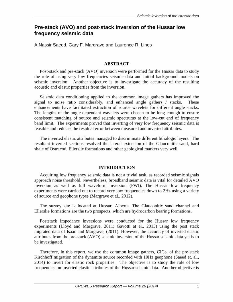
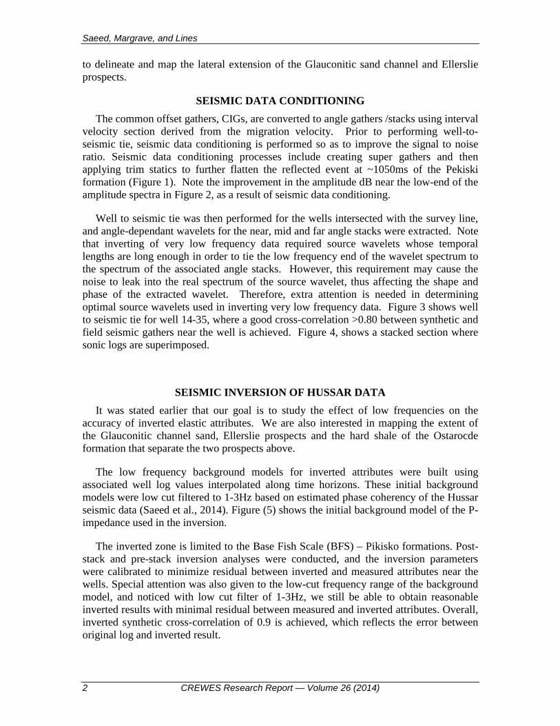
velocity section derived from the migration velocity. Prior to performing well-to- seismic tie, seismic data conditioning is performed so as to improve the signal to noise ratio. Seismic data conditioning processes include creating super gathers and then applying trim statics to further flatten the reflected event at ~1050ms of the Pekiski formation (Figure 1). Note the improvement in the amplitude dB near the low-end of the amplitude spectra in Figure 2, as a result of seismic data conditioning.

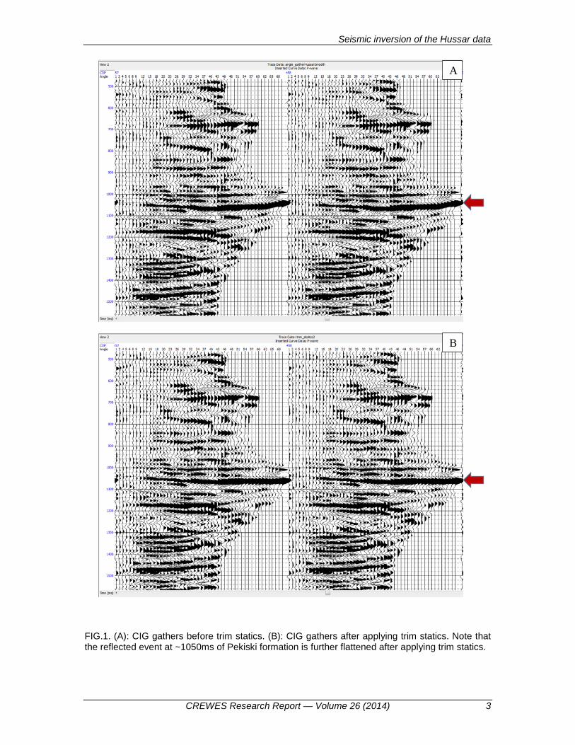
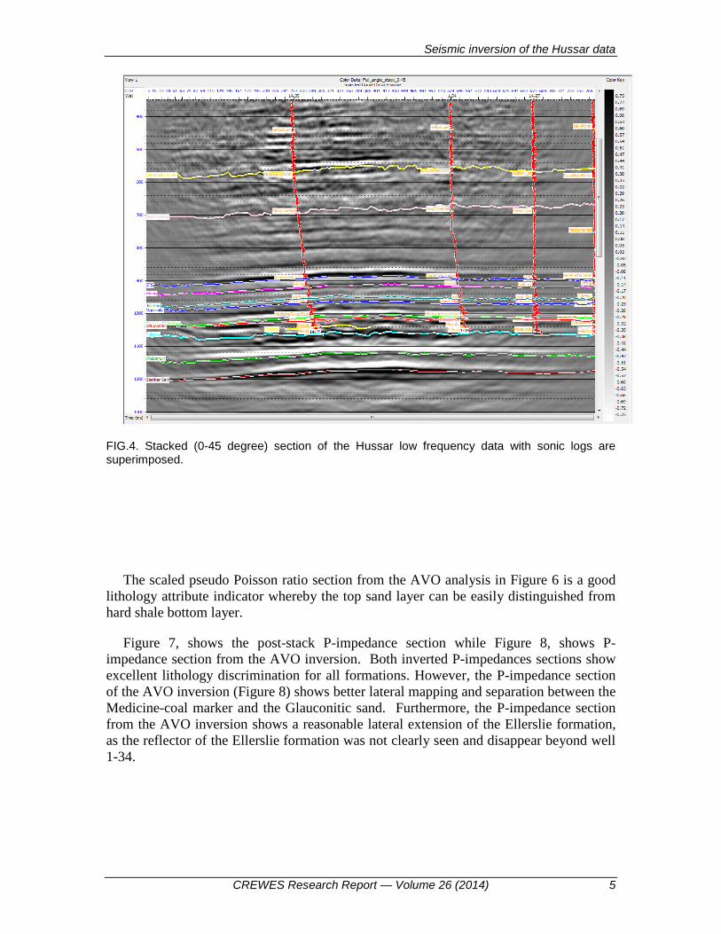
Well to seismic tie was then performed for the wells intersected with the survey line, and angle-dependant wavelets for the near, mid and far angle stacks were extracted. Note that inverting of very low frequency data required source wavelets whose temporal lengths are long enough in order to tie the low frequency end of the wavelet spectrum to the spectrum of the associated angle stacks. However, this requirement may cause the noise to leak into the real spectrum of the source wavelet, thus affecting the shape and phase of the extracted wavelet. Therefore, extra attention is needed in determining optimal source wavelets used in inverting very low frequency data. Figure 3 shows well to seismic tie for well 14-35, where a good cross-correlation >0.80 between synthetic and field seismic gathers near the well is achieved. Figure 4, shows a stacked section where sonic logs are superimposed.

SEISMIC INVERSION OF HUSSAR DATA It was stated earlier that our goal is to study the effect of low frequencies on the

accuracy of inverted elastic attributes. We are also interested in mapping the extent of the Glauconitic channel sand, Ellerslie prospects and the hard shale of the Ostarocde formation that separate the two prospects above.

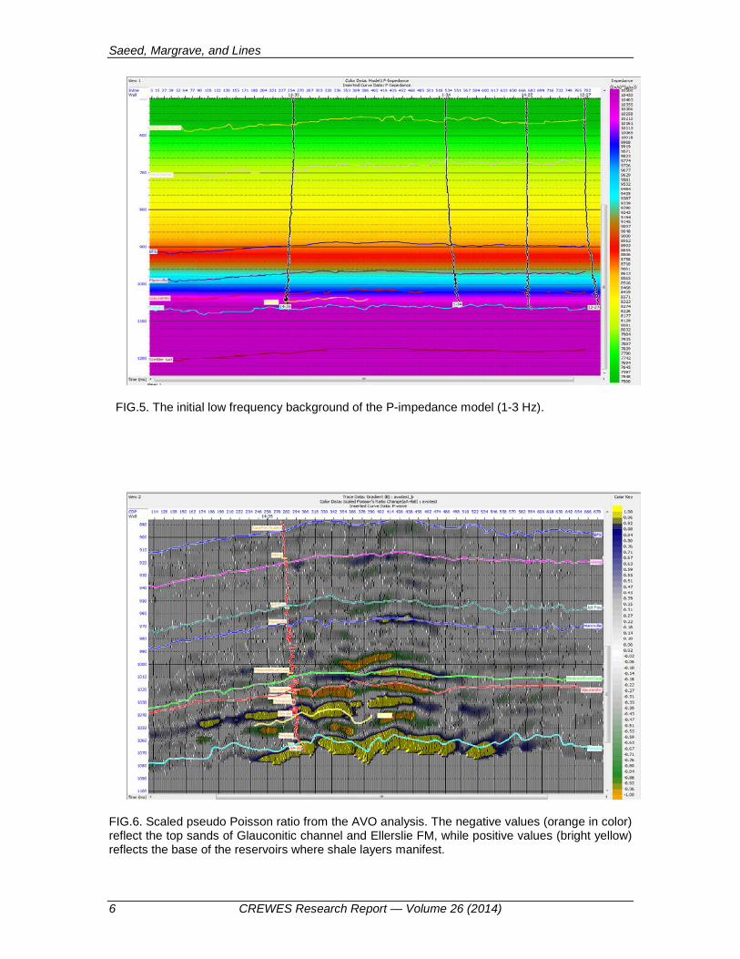
The low frequency background models for inverted attributes were built using associated well log values interpolated along time horizons. These initial background models were low cut filtered to 1-3Hz based on estimated phase coherency of the Hussar seismic data (Saeed et al., 2014). Figure (5) shows the initial background model of the P-impedance used in the inversion.

The inverted zone is limited to the Base Fish Scale (BFS) – Pikisko formations. Post-stack and pre-stack inversion analyses were conducted, and the inversion parameters were calibrated to minimize residual between inverted and measured attributes near the wells. Special attention was also given to the low-cut frequency range of the background model, and noticed with low cut filter of 1-3Hz, we still be able to obtain reasonable inverted results with minimal residual between measured and inverted attributes. Overall, inverted synthetic cross-correlation of 0.9 is achieved, which reflects the error between original log and inverted result.

2 CREWES Research Report — Volume 26 (2014)

Seismic inversion of the Hussar data

FIG.1. (A): CIG gathers before trim statics. (B): CIG gathers after applying trim statics. Note that the reflected event at ~1050ms of Pekiski formation is further flattened after applying trim statics.

B

A

CREWES Research Report — Volume 26 (2014) 3

Saeed, Margrave, and Lines

FIG.2. (A): Amplitude spectrum before applying seismic data conditioning. (B): Amplitude spectrum after applying seismic data conditioning. Note the improvement in the amplitude db at the low-end of the amplitude spectrum.

FIG.3. Well to seismic tie for well 14-35. Max Correlation of 0.82 is achieved at this well.

B

A

4 CREWES Research Report — Volume 26 (2014)

Seismic inversion of the Hussar data

FIG.4. Stacked (0-45 degree) section of the Hussar low frequency data with sonic logs are superimposed.

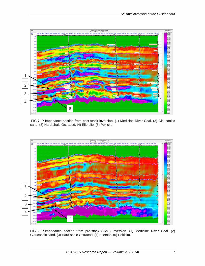
The scaled pseudo Poisson ratio section from the AVO analysis in Figure 6 is a good lithology attribute indicator whereby the top sand layer can be easily distinguished from hard shale bottom layer.

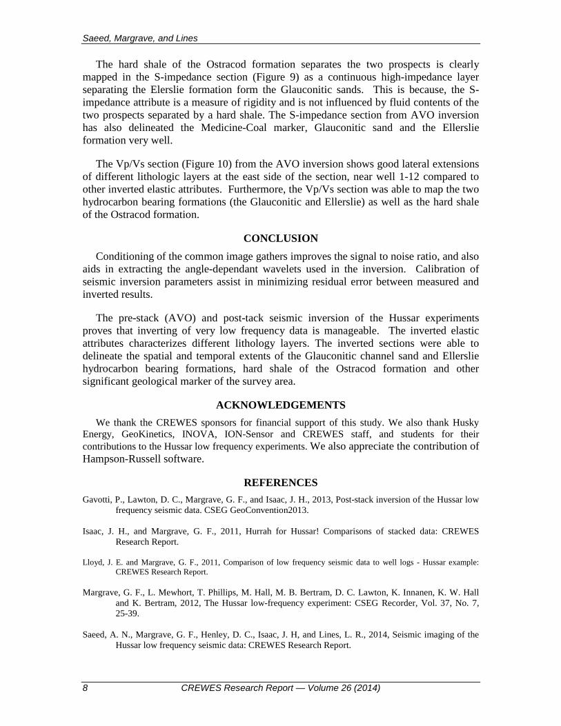
Figure 7, shows the post-stack P-impedance section while Figure 8, shows P-impedance section from the AVO inversion. Both inverted P-impedances sections show excellent lithology discrimination for all formations. However, the P-impedance section of the AVO inversion (Figure 8) shows better lateral mapping and separation between the Medicine-coal marker and the Glauconitic sand. Furthermore, the P-impedance section from the AVO inversion shows a reasonable lateral extension of the Ellerslie formation, as the reflector of the Ellerslie formation was not clearly seen and disappear beyond well 1-34.

CREWES Research Report — Volume 26 (2014) 5

Saeed, Margrave, and Lines

FIG.5. The initial low frequency background of the P-impedance model (1-3 Hz).

FIG.6. Scaled pseudo Poisson ratio from the AVO analysis. The negative values (orange in color) reflect the top sands of Glauconitic channel and Ellerslie FM, while positive values (bright yellow) reflects the base of the reservoirs where shale layers manifest.

6 CREWES Research Report — Volume 26 (2014)

Seismic inversion of the Hussar data

FIG.7. P-Impedance section from post-stack inversion. (1) Medicine River Coal. (2) Glauconitic sand. (3) Hard shale Ostracod. (4) Ellerslie. (5) Pekisko.

FIG.8. P-Impedance section from pre-stack (AVO) inversion. (1) Medicine River Coal. (2) Glauconitic sand. (3) Hard shale Ostracod. (4) Ellerslie. (5) Pekisko.

1

2

3

4

5

1

2

3

4

5

CREWES Research Report — Volume 26 (2014) 7

Saeed, Margrave, and Lines

The hard shale of the Ostracod formation separates the two prospects is clearly mapped in the S-impedance section (Figure 9) as a continuous high-impedance layer separating the Elerslie formation form the Glauconitic sands. This is because, the S-impedance attribute is a measure of rigidity and is not influenced by fluid contents of the two prospects separated by a hard shale. The S-impedance section from AVO inversion has also delineated the Medicine-Coal marker, Glauconitic sand and the Ellerslie formation very well.

The Vp/Vs section (Figure 10) from the AVO inversion shows good lateral extensions of different lithologic layers at the east side of the section, near well 1-12 compared to other inverted elastic attributes. Furthermore, the Vp/Vs section was able to map the two hydrocarbon bearing formations (the Glauconitic and Ellerslie) as well as the hard shale of the Ostracod formation.

CONCLUSION Conditioning of the common image gathers improves the signal to noise ratio, and also

aids in extracting the angle-dependant wavelets used in the inversion. Calibration of seismic inversion parameters assist in minimizing residual error between measured and inverted results.

The pre-stack (AVO) and post-tack seismic inversion of the Hussar experiments proves that inverting of very low frequency data is manageable. The inverted elastic attributes characterizes different lithology layers. The inverted sections were able to delineate the spatial and temporal extents of the Glauconitic channel sand and Ellerslie hydrocarbon bearing formations, hard shale of the Ostracod formation and other significant geological marker of the survey area.

ACKNOWLEDGEMENTS We thank the CREWES sponsors for financial support of this study. We also thank Husky

Energy, GeoKinetics, INOVA, ION-Sensor and CREWES staff, and students for their contributions to the Hussar low frequency experiments. We also appreciate the contribution of Hampson-Russell software.

REFERENCES Gavotti, P., Lawton, D. C., Margrave, G. F., and Isaac, J. H., 2013, Post-stack inversion of the Hussar low

frequency seismic data. CSEG GeoConvention2013. Isaac, J. H., and Margrave, G. F., 2011, Hurrah for Hussar! Comparisons of stacked data: CREWES

Research Report. Lloyd, J. E. and Margrave, G. F., 2011, Comparison of low frequency seismic data to well logs - Hussar example:

CREWES Research Report. Margrave, G. F., L. Mewhort, T. Phillips, M. Hall, M. B. Bertram, D. C. Lawton, K. Innanen, K. W. Hall

and K. Bertram, 2012, The Hussar low-frequency experiment: CSEG Recorder, Vol. 37, No. 7, 25-39.

Saeed, A. N., Margrave, G. F., Henley, D. C., Isaac, J. H, and Lines, L. R., 2014, Seismic imaging of the

Hussar low frequency seismic data: CREWES Research Report.

8 CREWES Research Report — Volume 26 (2014)

Seismic inversion of the Hussar data

FIG.9. S-Impedance section from the pre-stack (AVO) inversion. (1) Medicine River Coal. (2) Glauconitic sand. (3) Hard shale Ostracod. (4) Ellerslie. (5) Pekisko.

FIG.10. Vp/Vs section from the pre-stack (AVO) inversion. (1) Medicine River Coal. (2) Glauconitic sand. (3) Hard shale Ostracod. (4) Ellerslie. (5) Pekisko.

1

2

3

4

5

1

2

3

4

5

CREWES Research Report — Volume 26 (2014) 9