Predictable Patterns of Wintertime Surface Air Temperature in Northern Hemisphere and TheirPredictability Sources in the SEAS5

HONGDOU FAN,a,b LIN WANG,a,b YANG ZHANG,c YOUMIN TANG,d WANSUO DUAN,e AND LEI WANGa

aCenter for Monsoon System Research, Institute of Atmospheric Physics, Chinese Academy of Sciences, Beijing, ChinabCollege of Earth and Planetary Sciences, University of Chinese Academy of Sciences, Beijing, China

c School of Atmospheric Sciences, Nanjing University, Nanjing, ChinadEnvironmental Science and Engineering, University of Northern British Columbia, Prince George, British Columbia, Canada

e State Key Laboratory of Numerical Modeling for Atmospheric Sciences and Geophysical Fluid Dynamics,

Institute of Atmospheric Physics, Chinese Academy of Sciences, Beijing, China

(Manuscript received 13 July 2020, in final form 3 September 2020)

ABSTRACT: Based on 36-yr hindcasts from the fifth-generation seasonal forecast system of the European Centre for

Medium-RangeWeather Forecasts (SEAS5), themost predictable patterns of the wintertime 2-m air temperature (T2m) in

the extratropical Northern Hemisphere are extracted via the maximum signal-to-noise (MSN) empirical orthogonal

function (EOF) analysis, and their associated predictability sources are identified. The MSN EOF1 captures the warming

trend that amplifies over the Arctic but misses the associated warm Arctic–cold continent pattern. The MSN EOF2

delineates a wavelike T2m pattern over the Pacific–North America region, which is rooted in the tropical forcing of the

eastern Pacific-type El Niño–Southern Oscillation (ENSO). The MSN EOF3 shows a wavelike T2m pattern over the

Pacific–North America region, which has an approximately 908 phase difference from that associated with MSN EOF2,

and a loading center over midlatitude Eurasia. Its sources of predictability include the central Pacific-type ENSO and

Eurasian snow cover. TheMSNEOF4 reflects T2m variability surrounding the Tibetan Plateau, which is plausibly linked to

the remote forcing of the Arctic sea ice. The information on the leading predictable patterns and their sources of pre-

dictability is further used to develop a calibration scheme to improve the prediction skill of T2m. The calibrated prediction

skill in terms of the anomaly correlation coefficient improves significantly overmidlatitude Eurasia in a leave-one-out cross-

validation, implying a possible way to improve the wintertime T2m prediction in the SEAS5.

KEYWORDS: Climate prediction; ENSO; Snow cover; Sea ice; Surface temperature

1. Introduction

A reliable numerical weather forecast is usually limited to

about twoweeks (Bauer et al. 2015; Simmons andHollingsworth

2002) because of the chaotic dynamics of atmospheric circula-

tion (Lorenz 1963). The latter is also the main source of uncer-

tainties or noises in seasonal climate predictions. In contrast, the

existence of slowly varying atmospheric boundaries such as sea

surface temperature (SST), sea ice, and snow cover gives rise to

the feasibility of seasonal predictions (e.g., Charney and Shukla

1981;Doblas-Reyes et al. 2013;Kim et al. 2012) because they can

alter the likelihood of residence in atmosphere attractors and

thereby constrain the behaviors of the atmosphere on monthly

and longer time scales (Palmer 1993). Accordingly, the changes

in the atmosphere that are associated with these external factors

could be regarded as potentially predictable, whereas the re-

maining part of changes be regarded as potentially unpredict-

able in seasonal predictions.

Seasonal climate predictability has been widely investigated

regarding its spatial pattern and predictability sources using

dynamical models. Various approaches, such as signal-to-noise

metrics, have been proposed to quantify the seasonal predict-

ability (Rowell 1998). However, assessing seasonal predict-

ability using only one snapshot map makes it difficult to detect

the predictability sources because it lacks information on

temporal evolutions. Besides, certain spatial or temporal

structures may still be predictable with an optimized method

despite the low predictability in some areas (e.g., middle and

high latitudes). These inadequacies inspired a unified frame-

work for investigating predictability based on information

theory, in which the key approach is the maximized signal-to-

noise (MSN) empirical orthogonal function (EOF) analysis

(Allen and Smith 1997; DelSole and Tippett 2007). This

framework provides reliable estimations of predictability by

considering nonlinear factors, and it is convenient to explore

the spatial and temporal structures of predictability through

which the involved mechanism can be revealed. For example,

Tang et al. (2014, 2015) extracted the first and second pre-

dictable patterns of the North American surface air tempera-

ture via the MSN EOF analysis and attributed them to El

Niño–Southern Oscillation (ENSO) and global warming, re-

spectively. They further suggested that the first predictable

pattern is inherent to the most predictable patterns of the SST

and 500-hPa geopotential height. Scholars also use the MSN

EOF analysis to investigate the predictable patterns of mon-

soon precipitation (e.g., Liang et al. 2008; Zuo et al. 2013), the

tropical Indian Ocean SST (e.g., Wu and Tang 2019; Zhu et al.

2015), and the tropical Atlantic Ocean SST (e.g., Huang 2004),

among others, confirming the efficiency of the methodology.

Skillful seasonal prediction is crucial for Eurasia, where the

population density is high, and the natural hazard is frequent.Corresponding author: Lin Wang, wanglin@mail.iap.ac.cn

15 DECEMBER 2020 FAN ET AL . 10743

DOI: 10.1175/JCLI-D-20-0542.1

� 2020 American Meteorological Society. For information regarding reuse of this content and general copyright information, consult the AMS CopyrightPolicy (www.ametsoc.org/PUBSReuseLicenses).

Dow

nloaded from http://journals.am

etsoc.org/jcli/article-pdf/33/24/10743/5018954/jclid200542.pdf by Institute of Atmospheric Physics,C

AS, Lin Wang on 22 N

ovember 2020

In contrast to the climate of the Pacific–North America (PNA) re-

gion that is tightly related to ENSO (e.g., Horel and Wallace 1981;

Zhu et al. 2013, 2017; Tang et al. 2014, 2015), the Eurasian climate is

less influenced by ENSO on the interannual time scale because of

the complex processes and nonstationary footprint of ENSO (e.g.,

Ineson and Scaife 2008; Kumar et al. 1999; Wu andWang 2002; Jia

et al. 2017; Wang et al. 2008; Gong et al. 2019; Xie et al. 2016).

Meanwhile, the involvement of other active boundary forcing such

as snow cover and sea ice (e.g., Cohen and Fletcher 2007; Cohen

et al. 2014; Zuo et al. 2011, 2015) further increases the complexity

anduncertaintyof the seasonalpredictionoverEurasia.Moreover, it

remains unclear what the predictable patterns of the Eurasian cli-

mate and their sources are, motiving a careful investigation via the

state-of-the-art seasonal forecast systems. In this study, the leading

predictable patterns of thewintertime surface air temperature in the

whole extratropicalNorthernHemisphere,with the emphasis on the

Eurasian region, and their predictability sources are investi-

gated based on the outputs of the latest seasonal forecast sys-

tem of the European Centre for Medium-Range Weather

Forecasts (ECMWF). Given the above understanding, a cali-

bration scheme for seasonal prediction is proposed, which

turns out to evidently improve the prediction skill of surface air

temperature over the Eurasian region.

This paper is laid out as follows. Section 2 describes the da-

tasets and methodologies used in this study. Sections 3 and 4

identify the most predictable pattern of surface air temperature

in the extratropical Northern Hemisphere and their predict-

ability sources, respectively. Section 5 develops a calibration

scheme to improve the prediction skill of surface air temperature

by reinforcing the information of the leading predictable pat-

terns. Finally, section 6 concludes the key findings and discusses

some remaining issues.

2. Data and methods

The retrospective seasonal forecast (hindcast) data used in

this work are from the fifth-generation seasonal forecast sys-

tem (SEAS5; Johnson et al. 2019) of the ECMWF, which

consists of 25 ensemble members for the 36-yr hindcast period

1981–2016. The data have a horizontal resolution of 18 3 18 and11 vertical pressure levels extending from 925 to 10 hPa. As a

state-of-the-art seasonal forecast system, the SEAS5 is a fully

coupled general circulation models initialized on the first day

of every month and integrated continuously for seven months

(Johnson et al. 2019). It uses the Integrated Forecast System

(IFS) atmospheric model cycle 43r1 as its atmospheric com-

ponent and the Nucleus for European Modeling of the Ocean

(NEMO) model version 3.4.1 as its oceanic component. It also

includes a prognostic sea ice model, the Louvain-la-Neuve sea

ice model version 2 (LIM2), under the NEMO modeling

framework to improve the land–ice interactions. The atmo-

sphere, ocean, snow, sea ice, and other land fields are per-

turbed using an ensemble of data assimilations to represent

uncertainty in the initial state and ensemble spread. Compared

with its predecessor, System 4, the SEAS5 shows many im-

portant improvements, such as a better ENSO prediction skill.

More details can be found in Johnson et al. (2019) and the

SEAS5 user guide via https://www.ecmwf.int/sites/default/

files/medialibrary/2017-10/System5_guide.pdf. This study uses the

monthly mean hindcast data initialized on 1 November, which is the

most informative for the winter season. The use of the one-month

lead hindcasts is because it can balance between incorporating the

latest observed information into the seasonal forecast system and

guaranteeing enough time to take precautions for the coming season.

Several reanalysis and observational datasets are used to

evaluate and verify the results of hindcasts. The atmospheric

data are the monthly mean atmospheric reanalysis data from

the ERA-Interim dataset (Dee et al. 2011), which has a hori-

zontal resolution of 18 3 18 and 37 vertical pressure levels from

1000 to 1 hPa. The snow depth data are also from the ERA-

Interim dataset. The oceanic data are the observed monthly

mean SST and sea ice concentration (SIC) data from Hadley

Centre Sea Ice and Sea Surface Temperature dataset, version 1

(HadISST1; Rayner et al. 2003), which has a 18 3 18 resolutionand spans from 1870 to the present. These data are referred to

as ‘‘observation’’ hereafter.

This study focuses on the boreal winter that is defined as the

mean of December, January, and February. Climatology is de-

fined as the 36-yr (1981–2016) mean of the 25-member ensemble

mean in the SEAS5 and as the 36-yr mean in observational and

reanalysis datasets. The winter of 1981 refers to the 1981/82 win-

ter. The anomaly is calculated by removing the climatology from

the raw data. The two-tailed Student’s t test is used to evaluate the

significance of regression, correlation, linear trend, and the dif-

ferences between two linear trends (Santer et al. 2000). The Fisher

z transformation is used to evaluate the significance of differences

between two correlation coefficients (Conlon and Thomas 1993).

The most predictable patterns were extracted by applying

the MSN EOF (Allen and Smith 1997; DelSole and Tippett

2007; Tang et al. 2014) to the hindcast data from the SEAS5 as

follows. The MSN EOF method assumes that the ensemble

mean XM of seasonal mean anomalies X can be decomposed

into a forced (i.e., predictable) component XF and a random

(i.e., unpredictable) component (noise) XR:

XM5X

F1X

R. (1)

To find the optimal pattern (i.e., the leadingMSNEOFs) ofXF ,

the key procedure is to eliminate the spatial covariance of

noise by transforming the internal variation into spatially white

noise, known as the prewhitening transformation. In practice,

this approach is realized by performing the EOF analysis to the

ensemble deviations X0 5 X 2 XM:

CR5E

RL

RET

R , (2)

where CR is the covariance matrices of X0, LR is the diagonal

matrix ranking the eigenvalues in decreasing order, ER is the

eigenvectors, and the superscript T indicates the transpose of

the matrix. The prewhitened matrix X0M can be obtained by

projecting XM onto the kth highest-ranked eigenvectors E(k)R :

X0M 5 n1/2(L

(k)R )

21E(k)TR X

M, (3)

where n is the ensemble size. Note that k should be neither too big

nor too small to obtain the well-determined noise EOF space.

Here k is taken as 30 after a series of experiments, consistent with

10744 JOURNAL OF CL IMATE VOLUME 33

Dow

nloaded from http://journals.am

etsoc.org/jcli/article-pdf/33/24/10743/5018954/jclid200542.pdf by Institute of Atmospheric Physics,C

AS, Lin Wang on 22 N

ovember 2020

Huang (2004). Next, a singular value decomposition (SVD)

analysis is performed on the prewhitened matrix X0M :

X0M 5F0y0PT , (4)

where F0 is the left singular vectors, y0 is the diagonal matrix

ranking the eigenvalues in the decreasing orders, and the

highest-ranked right singular vector P is the optimized time

series we are looking for. Finally, the most predictable pattern

e (i.e., the optimal pattern with maximized signal-to-noise ra-

tio) can be obtained by projecting XM onto the optimized time

series PT. In this procedure, the weight in space is considered

(North et al. 1982), and the F test is used to evaluate the sig-

nificance of the MSN EOF (Huang 2004).

3. Leading predictable patterns of the surface airtemperature

Before analyzing the predictable patterns, we first evaluate the

prediction skill of the surface air temperature in the SEAS5.

Figure 1a shows the anomaly correlation coefficient (ACC) of the

wintermean air temperature 2m above the surface (T2mhereafter)

between the predicted ensemble mean and observation. The ACC

generally exceeds 0.3 over broad regions of the Northern

Hemisphere. High ACC is located in the regions to the south of

approximately 308N, North America between 408 and 608N, the

North Pacific, and the North Atlantic. It is surprising that the

ACC over the Arctic and Greenland is also high, especially over

the Barents Sea, possibly due to the inclusion of the sea ice

model in the SEAS5. In contrast, the ACC over the Eurasian

continent to the north of approximately 408N is very low and

even negative. This feature is also apparent in the zonal mean

ACC of T2m (Fig. 1b), which shows the lowest ACC between

408 and 708N. In addition to the linear ACC, the signal-to-noise

metrics (Rowell 1998) is also used to evaluate the predictability.

The signal-to-noise ratio of predicted T2m (Fig. 1c) shows a

similar pattern to the ACC with high values over the tropics,

subtropics, and the North Pacific (Fig. 1a). It is lower than 1 in

many regions of the Arctic and North Atlantic (Fig. 1c) despite

the high prediction skill (Fig. 1a). Nevertheless, a common

feature between the signal-to-noise ratio and theACC is the low

predictability and skill over the Eurasian continent, especially to

the north of 408N.

Figure 2 shows the four leading predictable patterns of the

winter mean T2m in the extratropical Northern Hemisphere

(208–898N) and the time series of their corresponding principal

components [MPCs hereafter;P inEq. (4)] obtained via theMSN

EOF analysis. The three patterns explain 53.2%, 15.9%, and

9.3% of the total variance, respectively. They all exceed the 5%

significance level based on the F test (Huang 2004), suggesting

that they are significantly predictablemodes. TheMSNEOF1

is a monopole warming pattern in the Northern Hemisphere,

and its maximum is over the Barents Sea (Fig. 2a). Its time

series (MPC1) shows a prominent upward trend with some

interannual variability (Fig. 2b), reminiscent of the global

warming signal. These results suggest that the MSN EOF1 is

likely a sign of the Arctic amplification (e.g., Fig. 2 in Cohen

et al. 2014). TheMSNEOF2 features warm anomalies over the

FIG. 1. (a) The ACC between observed and ensemble mean of the predicted winter mean

T2m for the period 1981–2016. (b) The zonal mean of the ACC. (c) The signal-to-noise ratio

of the predicted winter mean T2m, with values exceeding 1 highlighted by white contours

[contour interval (CI)5 3] in (c). Dots in (a) indicate the 5% significance level based on the

two-tailed Student’s t test.

15 DECEMBER 2020 FAN ET AL . 10745

Dow

nloaded from http://journals.am

etsoc.org/jcli/article-pdf/33/24/10743/5018954/jclid200542.pdf by Institute of Atmospheric Physics,C

AS, Lin Wang on 22 N

ovember 2020

northwestern North America and cold anomalies over the North

Pacific, subtropical North America, and the Barents Sea (Fig. 2d).

This pattern resembles that associatedwith the conventional eastern

Pacific (EP)ElNiño (e.g., Fig. 3 inBrönnimann2007) and implies its

plausible link toENSO.TheMSNEOF3manifests two cold centers

stretching from northern Eurasia to the subtropical central Pacific

andover easternNorthAmerica, respectively, and twowarmcenters

surroundingAlaska and Iceland (Fig. 2g). It has a thirdwarm center

over the Tibetan Plateau, but the spatial scale of this center is rela-

tively small. The MSN EOF3 resembles the leading mode of the

Eurasian surface air temperature on the interannual time scale over

Eurasia (e.g., Fig. 9a inWanget al. 2019) and the signal of the central

Pacific (CP)ENSOover thePNAregion (e.g., Figs. 3b and 3d inGu

and Adler 2019), implying its linkage to the CP ENSO and internal

variability over Eurasia. The MSN EOF4 is characterized by cold

anomalies centered over the Tibetan Plateau, the Bering Strait, the

Labrador Strait, andMexico andwarm anomalies centered over the

Barents Sea and midlatitude North America (Fig. 2j). This pattern

does not remind us of any known climate variability, but it might be

related to the forcing of the Tibetan Plateau or the changes in the

Arctic sea ice because of the locations of its centers. In the next

section, the atmospheric external forcing associated with the four

MSN EOFs are investigated in detail to reveal the possible pre-

dictability sources of these leading predictable patterns.

4. Predictability sources of the leading predictablepatterns

a. MSN EOF1

The MSN EOF1 dominates the Arctic T2m variability and

explains over 50% of the T2m variance over large areas of the

Arctic (Fig. 2c). Its monopole pattern with large loading over

the Barents Sea (Fig. 2a) and the upward trend during the past

decades (Fig. 2b) implies its possible origin from global

warming and the associated Arctic Amplification. To confirm

this inference, the long-term trend of winter mean T2m in the

SEAS5 was calculated, and it shows hemispheric warming with

centers over the Barents Sea and northeast North America

(Fig. 3a), which is almost identical to the MSN EOF1 (Fig. 2a).

The trend pattern in Fig. 3a was further projected onto the T2m

in the SEAS5 to get its time evolution (not shown), which has a

clear upward trend and is highly correlated to the MPC1 (r 50.98). These results confirm that the MSN EOF1 reflects the

global warming signal in the SEAS5. A comparison of the T2m

trend in the SEAS5 with that in the observation (Fig. 3b)

suggests that the SEAS5 underestimates the warming trends over

the Arctic and northeastern North America and fails to capture

the cooling trend over central Eurasia (Fig. 3c). The failure to

capture the observed warm Arctic–cold continent pattern

(Overland et al. 2011), also manifested as the EOF2 of the

observed T2m (eobs2 hereafter) over the extratropical Northern

Hemisphere (Fig. 3d), may be an essential reason for the low

prediction skill of T2mover centralEurasia in the SEAS5 (Fig. 1a).

The long-term trend in the near-surface temperature during

the past decades arises from the radiative forcing due to in-

creased greenhouse gas concentrations (e.g., Stocker et al.

2013). The amplified Arctic warming has been attributed to

local radiative effects, ice-albedo feedback, extratropical in-

fluences, and other processes (e.g., Chylek et al. 2009; Ding

et al. 2014; Graversen et al. 2008), whereas the continental

cooling may arise from the Arctic influences or the internal

variability within the climate system (e.g., Cohen et al. 2014,

2020). In the SEAS5, the greenhouse gas radiative forcing is

FIG. 2. (a) The MSN EOF1 of the winter mean T2m over the Northern Hemisphere (208–898N) in the SEAS5. (b) The normalized

principal components of theMSNEOF1 (i.e., MPC1). (c) The percent of variance (%) of the predicted T2m explained by theMSNEOF1.

(d)–(f),(g)–(i),(j)–(l) As in (a)–(c), but for the MSN EOF2, MSN EOF3, and MSN EOF4, respectively. The variance explained by the

MSN EOFs is denoted in the upper-right corner of (a), (d), (g), and (j).

10746 JOURNAL OF CL IMATE VOLUME 33

Dow

nloaded from http://journals.am

etsoc.org/jcli/article-pdf/33/24/10743/5018954/jclid200542.pdf by Institute of Atmospheric Physics,C

AS, Lin Wang on 22 N

ovember 2020

the zonally averaged seasonal varying climatology (Johnson

et al. 2019). It lacks the uneven spatial distribution and the

variation from year to year and thereby may cause the un-

derestimation of the T2m trend over the Arctic. Meanwhile,

the introduction of the LIM2 model introduces excess Arctic

sea ice and thereby cold bias over the Arctic in the SEAS5,

although it improves the skill in predicting the interannual

variability in sea ice (Johnson et al. 2019). This may be another

reason to underestimate the warming trend over theArctic and

thereby the cooling trend over Eurasia. Besides, the biases in

the winter temperature trends may also arise from the imper-

fection of models in simulating the snow cover variability and

the corresponding stratosphere–troposphere coupling (e.g.,

Cohen et al. 2012), but this is out of the scope of the current

study and needs further investigation in the future.

b. MSN EOF2

The MSN EOF2 dominates the T2m variability over the

PNA region and explains approximately 50% of the T2m

variance over the central North Pacific and western and central

North America (Fig. 2f). Its associated T2m anomalies re-

semble those during the conventional EP El Niño (Fig. 3 in

Brönnimann 2007) and imply its likely link to the EP ENSO.

To seek its sources of predictability, the predicted winter mean

SST is regressed onto the MPC2 of T2m, which shows a

prominent EP El Niño pattern. The SST warming is located in

the tropical central and eastern Pacific and the Indian Ocean,

and the SST cooling is over the subtropical Pacific (Fig. 4a).

The associated 500-hPa geopotential height anomalies manifest a

PNA-like wave train emanating from the subtropical central

Pacific (Fig. 4b). This wave train is equivalent barotropic (Fig. 4c),

and it could induce anomalous warming over northwestern North

America and cooling over the central North Pacific and south-

easternNorthAmerica via temperature advection (Fig. 4c). These

results suggest that the predictability of MSN EOF2 is very likely

rooted in the EP ENSO forcing. To further confirm this inter-

pretation, the conventional EOF analysis was applied to the

predicted winter mean SST in the tropical Pacific (308S–308N,

1108E–708W). The EOF1 of predicted SST shows a conventional

EP El Niño pattern (Fig. 4d), and its associated 500-hPa geo-

potential height anomalies (Fig. 4e) and T2m anomalies (Fig. 4f)

quite resemble those associated with the MSN EOF2 of T2m

(Figs. 4b,c). The correlation coefficient between MPC2 of T2m

and PC1 of SST, referred to as PC1SST, is 0.87, exceeding the 1%

significance level. Hence, the EP ENSO is a crucial source of

predictability for the T2m’s MSN EOF2. This result is

overall consistent with Tang et al. (2014) that ENSO’s SST

forcing dominates the most predictable T2m pattern over

the PNA region.

In addition to the EP ENSO forcing from the tropical

Pacific, the MSN EOF2 of T2m is also closely related to the

wintertime snow depth over North America (not shown). The

correlation coefficient between the MPC2 and the predicted

area-averaged (408–608N, 1708–608W) snow depth index is

pretty high (20.77). However, the regression of the wintertime

T2m onto the above snow depth index after removing the

ENSO signal does not showmuch significant signal in the PNA

region. Here, the removal of the ENSO signal is realized by

subtracting the regression coefficient of the predicted snow

depth index onto the simultaneous predicted Niño-3.4 index

from the predicted snow depth index (Wang et al. 2007; Chen

et al. 2013). This result suggests that the North America snow

anomalies are more like a passive response to EP ENSO rather

than an independent atmospheric external forcing for the

MSN EOF2 of T2m.

c. MSN EOF3

The MSN EOF3 mainly influences the T2m variability over

the North Pacific and Eurasia, and it explains approximately

25% and 15% of the T2m variance over the northwestern

Pacific and central northern Eurasia (Fig. 2i), respectively. Its

associated T2m anomalies are similar to those associated with

the CP ENSO over the PNA region (e.g., Figs. 3b and 3d in

Gu and Adler 2019). It is directly induced by a barotropic

FIG. 3. Linear trends of the (a) predicted and (b) observed T2m [8C (10 yr)21] during winters 1981–2016.

(c) Differences between (a) and (b). (d) The EOF2 of the observed winter mean T2m over the extratropical

NorthernHemisphere (208–898N) derived from the period 1981–2016. Dots denote the linear trends, the difference

between the linear trends and the linear regression coefficients exceed the 5% significance level in (a)–(d),

respectively.

15 DECEMBER 2020 FAN ET AL . 10747

Dow

nloaded from http://journals.am

etsoc.org/jcli/article-pdf/33/24/10743/5018954/jclid200542.pdf by Institute of Atmospheric Physics,C

AS, Lin Wang on 22 N

ovember 2020

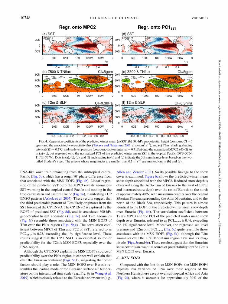
PNA-like wave train emanating from the subtropical central

Pacific (Fig. 5b), which has a rough 908 phase difference from

that associated with the MSN EOF2 (Fig. 4b). Linear regres-

sion of the predicted SST onto the MPC3 reveals anomalous

SST warming in the tropical central Pacific and cooling in the

tropical western and eastern Pacific (Fig. 5a), manifesting a CP

ENSO pattern (Ashok et al. 2007). These results suggest that

the third predictable pattern of T2m likely originates from the

SST forcing of the CP ENSO. The CP ENSO is captured by the

EOF2 of predicted SST (Fig. 5d), and its associated 500-hPa

geopotential height anomalies (Fig. 5e) and T2m anomalies

(Fig. 5f) resemble those associated with the MSN EOF3 of

T2m over the PNA region (Figs. 5b,c). The correlation coef-

ficient between MPC3 of T2m and PC2 of SST, referred to as

PC2SST, is 0.75, exceeding the 1% significance level. These

results suggest that the CP ENSO is an essential source of

predictability for the T2m’s MSN EOF3, especially over the

PNA region.

Although the CPENSO explains theMSNEOF3’s source of

predictability over the PNA region, it cannot well explain that

over the Eurasian continent (Figs. 5c,f), suggesting that other

factors should play a role. The MSN EOF3 over Eurasia re-

sembles the leading mode of the Eurasian surface air temper-

ature on the interannual time scale (e.g., Fig. 9a in Wang et al.

2019), which is closely related to the Eurasian snow cover (e.g.,

Allen and Zender 2011). So its possible linkage to the snow

cover is examined. Figure 6a shows the predicted winter mean

snow depth associated with the MPC3. Reduced snow depth is

observed along the Arctic rim of Eurasia to the west of 1308Eand increased snow depth over the rest of Eurasia to the north

of approximately 408N, with maximum centers over the central

Siberian Plateau, surrounding the Altai Mountains, and to the

north of the Black Sea, respectively. This pattern is almost

identical to the EOF1 of the predicted winter mean snow depth

over Eurasia (Fig. 6b). The correlation coefficient between

T2m’s MPC3 and the PC1 of the predicted winter mean snow

depth over Eurasia, referred to as PC1snow, is 0.46, exceeding

the 1% significance level. Moreover, the regressed sea level

pressure and T2m onto PC1snow (Fig. 6c) quite resemble those

associated with the MSN EOF3 (Fig. 5c), although the T2m

anomalies over the Ural Mountains region have smaller mag-

nitude (Figs. 5c and 6c). These results suggest that the Eurasian

snow cover is an essential source of predictability for the T2m’s

MSN EOF3 over Eurasia.

d. MSN EOF4

Compared with the first three MSN EOFs, the MSN EOF4

explains less variance of T2m over most regions of the

Northern Hemisphere except over subtropical Africa and Asia

(Fig. 2l), where it accounts for approximately 30% of the

FIG. 4. Regression coefficients of the predictedwintermean (a) SST, (b) 500-hPa geopotential height (contours; CI5 5

gpm) and the associated wave-activity flux (Takaya and Nakamura 2001; arrow; m2 s22), and (c) T2m [shading; shading

interval (SI)5 0.28C] and sea level pressure (contours; contour interval5 0.3 hPa) onto the normalizedMPC2. (d)–(f)As

in (a)–(c), but regressed onto the normalized PC1 of the predicted winter mean SST in the tropical Pacific (308S–308N,

1108E–708W). Dots in (a), (c), (d), and (f) and shading in (b) and (c) indicate the 5% significance level based on the two-

tailed Student’s t test. The arrows whose magnitudes are smaller than 0.2m2 s22 are masked out in (b) and (e).

10748 JOURNAL OF CL IMATE VOLUME 33

Dow

nloaded from http://journals.am

etsoc.org/jcli/article-pdf/33/24/10743/5018954/jclid200542.pdf by Institute of Atmospheric Physics,C

AS, Lin Wang on 22 N

ovember 2020

variance. It delineates a seesaw-like anomalous T2m pattern,

with significant cooling surrounding the Tibetan Plateau and

warming over the Barents–Kara Seas (Fig. 7b). This temper-

ature pattern is associated with a midtropospheric wavelike

anomaly from the Arctic to the Tibetan Plateau (Fig. 7b),

implying its plausible linkage to the Arctic. Inspection of the

Arctic sea ice indicates that theMSNEOF4 is closely related to

changes in the winter mean SIC over the Barents Sea and

Norwegian Sea (Fig. 7a). This MSN EOF4-related SIC pat-

tern is almost identical to the EOF1 of the winter mean SIC

over the Arctic (708–898N) (Fig. 7c). The correlation coeffi-

cient between the MPC4 of T2m and the PC1 of the winter

mean Arctic SIC, referred to as PC1SIC, is 20.51, exceeding

the 1% significance level. However, the regressed T2m onto

PC1SIC (Fig. 7d) shows an opposite sign to that onto the

MPC4 surrounding the Tibetan Plateau, although they are

quite alike over theArctic region (Fig. 7b). Note the observed

wintertime Arctic and Tibetan T2m vary in phase (e.g., Gu

et al. 2018; Zhang et al. 2019), consistent with Fig. 7d,

not Fig. 7b. Hence, this result implies the uncertain role of

the Arctic SIC in the sources of the predictability for the

MSN EOF4.

The cause-and-effect relationship between theArctic sea ice

and the midlatitude climate is complex and has not reached a

consensus (Cohen et al. 2020). This complexity is also reflected

in the first four MSN EOFs, all of which show similar patterns

over the Barents Sea and different patterns over the midlati-

tudes (Figs. 2a,d,g,j). The correlation coefficients between the

PC1SIC and the four MPCs all exceed the 5% significance level

(Table 1), and the highest correlation is between PC1SIC and

MPC4. This result implies that the plausible forcing of the

Arctic sea ice on the wintertime T2m, if any, is most realized

through the MSN EOF4 although the MSN EOF4 cannot re-

produce the observed Arctic–Tibetan connection of T2m, as

discussed in the previous paragraph. Nevertheless, the T2m

signals in Figs. 7b and 7d are consistent surrounding the Ural

Mountain region. This result suggests that the Arctic SIC may

serve as a source of predictability for the T2m variations sur-

rounding the Ural Mountain.

5. Improved predictions over Eurasia by incorporatingthe predictable patterns

It is essential to identify the leading predictable patterns and

their sources of predictability because it helps to understand

the T2m variability in the SEAS5. It will be practically bene-

ficial if such understanding can be used to improve the pre-

diction skill. To this end, a scheme is developed as an attempt

to improve the prediction skill of T2m in the SEAS5. The as-

sumption behind this scheme is that the model can capture the

sources of predictability for T2m and that it is incapable of

predicting T2m skillfully because it misrepresents the atmo-

spheric responses to these external forcing. Hence, the pre-

diction skill may be improved by incorporating the information

related to the leading predictable patterns in a statistical

manner. In practice, the prediction is reconstructed based on

FIG. 5. (a)–(c) As in Figs. 4a–c, but for the MPC3. (d)–(f) As in Figs. 4d–f, but for the PC2 of the SST. The arrows

whose magnitudes are smaller than 0.05m2 s22 are masked out in (b) and (e).

15 DECEMBER 2020 FAN ET AL . 10749

Dow

nloaded from http://journals.am

etsoc.org/jcli/article-pdf/33/24/10743/5018954/jclid200542.pdf by Institute of Atmospheric Physics,C

AS, Lin Wang on 22 N

ovember 2020

the spatial patterns of leading predictable patterns and time

series of the identified predictability sources:

T5�4

i51

Ti

5�4

i51

eiti

5 eobs2 MPC1

T2m1e

2PC1

SST1e

3PC1

snow1e

4PC1

SIC, (5)

where Ti is the reconstructed T2m prediction based on the ith

leading predictable pattern ei and the time series of the cor-

responding predictability source ti. The second to fourth e are

exactly the spatial patterns of the second to fourth MSN EOFs

(Figs. 2d,g,j), and their corresponding ti are the PC1SST,

PC1snow, and PC1SIC discussed in sections 4b, 4c, and 4d, re-

spectively. One exception is for e1 and t1. Here the spatial

pattern of MSN EOF1 (Fig. 2a) is not used in the recon-

struction because it underestimates the warming trend over

the Arctic and misses the cooling trend over Eurasia

(Fig. 3c). Instead, the observed EOF2 of the extratropical

wintertime T2m (eobs2 ; Fig. 3d) is used. The eobs

2 , not the

pattern of T2m’s trend (Fig. 3b), is used for the easier ex-

tracting patterns in cross-validation. More importantly, the

eobs2 can well represent the observed pattern of T2m’s trend

(Fig. 3b), and its time series is highly correlated (r 5 0.92) to

that of the observed T2m’s trend, which is obtained by pro-

jecting the observed T2m onto the observed T2m’s trend

(Fig. 3b). Here t1 equals MPC1T2m that is obtained by pro-

jecting the MSN EOF1 onto the predicted T2m over the ex-

tratropical Northern Hemisphere (208–898N). The use of

MPC1T2m guarantees that the time series of t1 can be gener-

ated within the model for the prediction purpose, although

the spatial pattern is replaced by the observation (eobs2 ). The

PC2SST was not used to replace t3 because the focus is on

Eurasia, where the prediction skill is low (Fig. 1a), and the in-

fluence of the CP ENSO is relatively weak (Fig. 5f). The am-

plitudes of ti are adjusted prior to the reconstruction to match

their substitutes using the standard deviations of the substitutes.

To test the capability of the calibration scheme, the leave-

one-out cross-validation method (Michaelsen 1987) was em-

ployed. This method reconstructs the wintertime T2m in a

specific year based on the remaining years other than this year

using the forecast model in Eq. (5). For example, the MSN

EOF and EOF analyses are performed during the years 1981–

90 combined with 1992–2016, and the resultant information

is used to reconstruct the T2m in the year 1991. The above

approaches are repeated so that T2m in every year during

1981–2016 is reconstructed. Figure 8a shows the ACC between

observed and reconstructed T2m using the first four MSN

EOFs in the leave-one-out cross-validation. The ACC gener-

ally exceeds 0.3 over large areas of midlatitude Eurasia. This

performance is in sharp contrast to the low and even negative

ACC based on the ensemble mean of direct model outputs in

this region (Fig. 1a). It suggests that the reconstructed T2m

shows apparent improvement in the prediction skill over

midlatitude Eurasia (e.g., between 458 and 708N) compared

with the direct ensemble mean of the SEAS5, especially in

regions to the east of Ural Mountains (Fig. 8b). The im-

provement of the ACC (Fig. 8b) projects well onto the pattern

of the MSN EOF3 (Fig. 2g) and eobs2 (Fig. 3d), implying its

primary origins from the Eurasian snow cover and the warm

Arctic–cold continent pattern. Inspection of the effects of in-

dividual factors on the ACC confirms this inference (Fig. 9).

Meanwhile, it is noteworthy that the prediction skill of re-

constructed T2m is worse than the direct ensemble means of

the SEAS5 in most of the Northern Hemisphere other than

Eurasia. On the one hand, this result is understandable because

the performance of the SEAS5 is already good in regions

outside Eurasia. It is insufficient to use only four predictable

modes for the reconstruction in these regions. On the other

hand, this result suggests that it is very likely an efficient way to

replace the model predicted T2mwith reconstructed T2m over

midlatitude Eurasia to improve the prediction skill of winter-

time T2m in the SEAS5.

FIG. 6. Regression coefficients of the predicted winter mean

snow depth onto the normalized (a) MPC3 and (b) PC1snow, the

time series of the EOF1 of winter mean snow depth over Eurasia

(208–1308E, 458–758N). (c) As in (b), but for the predicted winter

mean T2m (shading; shading interval 5 0.18C) and sea level pres-

sure (contours; contour interval 5 0.1 hPa). Dots indicate the 5%

significance level based on the two-tailed Student’s t test.

10750 JOURNAL OF CL IMATE VOLUME 33

Dow

nloaded from http://journals.am

etsoc.org/jcli/article-pdf/33/24/10743/5018954/jclid200542.pdf by Institute of Atmospheric Physics,C

AS, Lin Wang on 22 N

ovember 2020

6. Conclusions and discussion

Slow-varying atmospheric boundaries are the main sources

of seasonal climate predictions, and their footprints on climate

variables may be captured as predictable patterns. Based on

the 36-yr hindcast data from the SEAS5, the latest ECMWF

seasonal forecast system, this study extracted the leading pre-

dictable patterns of the extratropical Northern Hemisphere

T2m in boreal winter via the MSN EOF analysis and identified

their sources of predictability. The MSN EOF1, the dominant

predictable pattern, explains 53.2% of the total variance and

reflects the long-term warming trend of T2m. The SEAS5

underestimates the observed magnitude of the warming trend

and misses the observed warm Arctic–cold continent pattern.

The MSN EOF2 and MSN EOF3, which explain 15.9% and

9.3% of the total variance, respectively, manifest a wavelike

T2m pattern over the PNA region. Their sources of predict-

ability can be traced to the tropical forcing associated with the

EP and CP ENSO, respectively. In addition, the MSN EOF3

has large loading over the midlatitude Eurasia that cannot be

explained by the CP ENSO. Inspection suggests that this T2m

variability over Eurasia can be attributed to the forcing from the

Eurasian snow. The MSN EOF4 explains only 5.1% of the total

variance, and it delineates T2m variability surrounding the

Tibetan Plateau. Its source of predictability can be partially

traced to the Arctic sea ice in the Barents and Norwegian Seas

with some uncertainty. The SEAS5’s prediction skill of the

wintertime T2m is overall good in the extratropical Northern

Hemisphere except over midlatitude Eurasia. A calibration

scheme is developed as an attempt to improve the prediction

skill of T2m by reinforcing the information of the first fourMSN

EOFs and their sources of predictability. It reveals that the

prediction skill in terms of the ACC improves significantly over

midlatitude Eurasia in a leave-one-out cross-validation. This

result confirms the importance of the predictable patterns and

their sources in the seasonal predictions and implies a possible

way to improve the wintertime T2m prediction over Eurasia.

In this study, the wintertime atmospheric external forcing

was identified as a source of predictability for the leading

predictable patterns. This approach is usually acceptable for

remote forcing such as that from ENSO, but it may be ques-

tioned for the in situ atmospheric boundaries such as midlati-

tude snow cover and sea ice because of their strong

interactions with the atmosphere. On the one hand, such

questions are reasonable to some extent because there are

FIG. 7. Regression coefficients of the predicted winter mean (a) SIC and (b) T2m (shading; shading interval 50.02) and 500-hPa geopotential height (contour; contour interval5 1 gpm) onto the normalizedMPC4. (c),(d)As in

(a) and (b), but regressed onto the normalized PC1 of the predicted winter mean SIC in theArctic (708–898N). Dots

indicate the 5% significance level of the (top) SIC and (bottom) T2m based on the two-tailed Student’s t test. The

regression coefficients in (c) and (d) have been multiplied by 21 for the convenience of comparison.

TABLE 1. Correlation coefficients between the predicted PC1SICand the fourMPCs duringwinters 1981–2016.Values exceeding the

5% and 1% significance levels based on the two-tailed Student’s t

test are denoted by one and two asterisks, respectively (* and **).

MPC1 MPC2 MPC3 MPC4

PC1SIC 20.40* 0.33* 20.40* 20.51**

15 DECEMBER 2020 FAN ET AL . 10751

Dow

nloaded from http://journals.am

etsoc.org/jcli/article-pdf/33/24/10743/5018954/jclid200542.pdf by Institute of Atmospheric Physics,C

AS, Lin Wang on 22 N

ovember 2020

indeed interactions between the extratropical atmosphere and

the underlying snow cover or sea ice. Strictly speaking, the sig-

nals of wintertime Eurasia snow cover and Arctic sea ice used in

this study are the results of these interactions.On the other hand,

it is reasonable to regard these wintertime signals as relative

external forcing because they indeed force the atmosphere in the

interaction with the atmosphere. As a result, reconstructed T2m

by incorporating these forcing signals improves the prediction

skill significantly over Eurasia. Nevertheless, it is noteworthy

that the SEAS5 is a coupledmodel that does not have boundary

forcing. Hence, the identified atmospheric external forcing and,

thereby, the predictability sources should finally be from initial

fields of long memory. It is meaningful to track these initial

conditions for the predictable patterns, but it cannot be done in

this study because of the unavailability of related data. Last but

not least, this study is based on the SEAS5. It would be mean-

ingful to examine the robustness of the results in other seasonal

forecast systems, and this will be done in the future.

Acknowledgments. We thank the three anonymous re-

viewers for their valuable comments and suggestions. This

work was supported by the National Key R&D Program of

China (2018YFC1506001) and the National Natural Science

Foundation of China (41925020, 41721004). We thank Dr.

Lijuan Hua for providing literature on significance tests on

linear trends.

FIG. 8. (a) The prediction skill of reconstructed T2m using the first four MSN EOFs measured by the ACC

between observed T2m and reconstructed T2m. See text for details of the reconstruction. (b) The difference of

ACC between reconstructed T2m prediction skill (Fig. 8a) and direct T2m prediction skill in the SEAS5

(Fig. 2a). Dots indicate the 5% and 10% significance level based on the two-tailed Student’s t test in (a) and (b),

respectively.

FIG. 9. The ACC between observed T2m and reconstructed T2m using the (a) first, (b) second, (c) third, and

(d) fourth MSN EOF alone. Dots indicate the 5% significance level based on the two-tailed Student’s t test.

10752 JOURNAL OF CL IMATE VOLUME 33

Dow

nloaded from http://journals.am

etsoc.org/jcli/article-pdf/33/24/10743/5018954/jclid200542.pdf by Institute of Atmospheric Physics,C

AS, Lin Wang on 22 N

ovember 2020

REFERENCES

Allen, M. R., and L. A. Smith, 1997: Optimal filtering in singular

spectrum analysis. Phys. Lett., 234A, 419–428, https://doi.org/

10.1016/S0375-9601(97)00559-8.

Allen, R. J., and C. S. Zender, 2011: Forcing of the Arctic

Oscillation by Eurasian snow cover. J. Climate, 24, 6528–6539,

https://doi.org/10.1175/2011JCLI4157.1.

Ashok, K., S. K. Behera, S. A. Rao, H.Weng, and T. Yamagata, 2007:

ElNiñoModoki and its possible teleconnection. J.Geophys. Res.,

112, C11007, https://doi.org/10.1029/2006JC003798.

Bauer, P., A. Thorpe, and G. Brunet, 2015: The quiet revolution of

numerical weather prediction. Nature, 525, 47–55, https://

doi.org/10.1038/nature14956.

Brönnimann, S., 2007: Impact of El Niño–Southern Oscillation on

European climate.Rev. Geophys., 45, RG3003, https://doi.org/

10.1029/2006RG000199.

Charney, J. G., and J. Shukla, 1981: Predictability of monsoons.

Monsoon Dynamics, J. Lighthill and R. P. Pearce, Eds.,

Cambridge University Press, 99–109.

Chen, W., J. Feng, and R. Wu, 2013: Roles of ENSO and PDO in

the link of the East Asian winter monsoon to the following

summer monsoon. J. Climate, 26, 622–635, https://doi.org/

10.1175/JCLI-D-12-00021.1.

Chylek, P., C. K. Folland, G. Lesins, M. K. Dubey, and M. Wang,

2009: Arctic air temperature change amplification and the

Atlantic multidecadal oscillation. Geophys. Res. Lett., 36,

L14801, https://doi.org/10.1029/2009GL038777.

Cohen, J., and C. Fletcher, 2007: Improved skill of Northern

Hemisphere winter surface temperature predictions based on

land–atmosphere fall anomalies. J. Climate, 20, 4118–4132,

https://doi.org/10.1175/JCLI4241.1.

——, J. C. Furtado, M. Barlow, V. A. Alexeev, and J. E. Cherry,

2012: Asymmetric seasonal temperature trends.Geophys. Res.

Lett., 39, L04705, https://doi.org/10.1029/2011GL050582.

——, and Coauthors, 2014: Recent Arctic amplification and ex-

treme mid-latitude weather. Nat. Geosci., 7, 627–637, https://

doi.org/10.1038/ngeo2234.

——, and Coauthors, 2020: Divergent consensuses on Arctic am-

plification influence on midlatitude severe winter weather. Nat.

Climate Change, 10, 20–29, https://doi.org/10.1038/s41558-019-

0662-y.

Conlon, M., and R. G. Thomas, 1993: The power function for

Fisher’s exact test. J. Roy. Stat. Soc., 42C, 258–260, https://

doi.org/10.2307/2347431.

Dee, D. P., and Coauthors, 2011: The ERA-Interim reanalysis:

Configuration and performance of the data assimilation sys-

tem.Quart. J. Roy. Meteor. Soc., 137, 553–597, https://doi.org/

10.1002/qj.828.

DelSole, T., andM.K. Tippett, 2007: Predictability: Recent insights

from information theory. Rev. Geophys., 45, RG4002, https://

doi.org/10.1029/2006RG000202.

Ding, Q., J. M. Wallace, D. S. Battisti, E. J. Steig, A. J. Gallant,

H. J. Kim, and L. Geng, 2014: Tropical forcing of the recent

rapid Arctic warming in northeastern Canada and Greenland.

Nature, 509, 209–212, https://doi.org/10.1038/nature13260.Doblas-Reyes, F. J., J. García-Serrano, F. Lienert, A. P. Biescas,

and L. R. L. Rodrigues, 2013: Seasonal climate predictability

and forecasting: Status and prospects. Wiley Interdiscip. Rev.:

Climate Change, 4, 245–268, https://doi.org/10.1002/wcc.217.

Gong, H., L. Wang, and W. Chen, 2019: Recently strengthened

influence of ENSO on the wintertime East Asian surface air

temperature. Atmosphere, 10, 720, https://doi.org/10.3390/

atmos10110720.

Graversen, R. G., T. Mauritsen, M. Tjernstrom, E. Kallen, and

G. Svensson, 2008: Vertical structure of recent Arctic warm-

ing. Nature, 451, 53–56, https://doi.org/10.1038/nature06502.Gu, G. J., and R. F. Adler, 2019: Precipitation, temperature, and

moisture transport variations associated with two distinct

ENSO flavors during 1979–2014.Climate Dyn., 52, 7249–7265,

https://doi.org/10.1007/s00382-016-3462-3.

Gu, S., Y. Zhang, Q. Wu, and X.-Q. Yang, 2018: The linkage be-

tween Arctic sea ice and midlatitude weather: In the per-

spective of energy. J. Geophys. Res. Atmos., 123, 11 536–

11 550, https://doi.org/10.1029/2018JD028743.

Horel, J. D., and J. M. Wallace, 1981: Planetary-scale atmospheric phe-

nomena associated with the Southern Oscillation.Mon. Wea. Rev.,

109, 813–829, https://doi.org/10.1175/1520-0493(1981)109,0813:

PSAPAW.2.0.CO;2.

Huang, B., 2004: Remotely forced variability in the tropical

Atlantic Ocean. Climate Dyn., 23, 133–152, https://doi.org/

10.1007/s00382-004-0443-8.

Ineson, S., and A. A. Scaife, 2008: The role of the stratosphere in

the European climate response to El Niño.Nat. Geosci., 2, 32–

36, https://doi.org/10.1038/ngeo381.

Jia, L., and Coauthors, 2017: Seasonal prediction skill of northern

extratropical surface temperature driven by the stratosphere.

J.Climate,30, 4463–4475, https://doi.org/10.1175/JCLI-D-16-0475.1.

Johnson, S. J., and Coauthors, 2019: SEAS5: The new ECMWF

seasonal forecast system. Geosci. Model Dev., 12, 1087–1117,

https://doi.org/10.5194/gmd-12-1087-2019.

Kim,H.-M., P. J.Webster, and J.A. Curry, 2012: Seasonal prediction

skill of ECMWF system 4 and NCEP CFSv2 retrospective

forecast for the Northern Hemisphere winter.Climate Dyn., 39,

2957–2973, https://doi.org/10.1007/s00382-012-1364-6.

Kumar,K.K.,B.Rajagopalan, andM.A.Cane, 1999:On theweakening

relationship between the Indianmonsoon andENSO. Science, 284,

2156–2159, https://doi.org/10.1126/science.284.5423.2156.

Liang, J., S. Yang, Z.-Z. Hu, B. Huang, A. Kumar, and Z. Zhang,

2008: Predictable patterns of the Asian and Indo-Pacific

summer precipitation in the NCEP CFS. Climate Dyn., 32,

989–1001, https://doi.org/10.1007/s00382-008-0420-8.

Lorenz, E. N., 1963: Deterministic nonperiodic flow. J. Atmos. Sci.,

20, 130–141, https://doi.org/10.1175/1520-0469(1963)020,0130:

DNF.2.0.CO;2.

Michaelsen, J., 1987: Cross-validation in statistical climate forecast

models. J. Climate Appl. Meteor., 26, 1589–1600, https://doi.org/

10.1175/1520-0450(1987)026,1589:CVISCF.2.0.CO;2.

North, G. R., T. L. Bell, R. F. Cahalan, and F. J. Moeng, 1982:

Sampling errors in the estimation of empirical orthogonal

functions. Mon. Wea. Rev., 110, 699–706, https://doi.org/

10.1175/1520-0493(1982)110,0699:SEITEO.2.0.CO;2.

Overland, J. E., K. R.Wood, andM.Wang, 2011:WarmArctic–cold

continents: Climate impacts of the newly openArctic Sea.Polar

Res., 30, 15 787, https://doi.org/10.3402/polar.v30i0.15787.

Palmer, T. N., 1993: Extended-range atmospheric prediction and the

Lorenzmodel.Bull.Amer.Meteor. Soc., 74, 49–65, https://doi.org/

10.1175/1520-0477(1993)074,0049:ERAPAT.2.0.CO;2.

Rayner, N. A., D. E. Parker, E. B. Horton, C. K. Folland, L. V.

Alexander,D. P.Rowell, E.C.Kent, andA.Kaplan, 2003:Global

analyses of sea surface temperature, sea ice, and night marine air

temperature since the late nineteenth century. J. Geophys. Res.,

108, 4407, https://doi.org/10.1029/2002JD002670.

Rowell, D. P., 1998: Assessing potential seasonal predict-

ability with an ensemble of multidecadal GCM simula-

tions. J.Climate, 11, 109–120, https://doi.org/10.1175/1520-0442(1998)

011,0109:APSPWA.2.0.CO;2.

15 DECEMBER 2020 FAN ET AL . 10753

Dow

nloaded from http://journals.am

etsoc.org/jcli/article-pdf/33/24/10743/5018954/jclid200542.pdf by Institute of Atmospheric Physics,C

AS, Lin Wang on 22 N

ovember 2020

Santer, B. D., T. M. L. Wigley, J. S. Boyle, D. J. Gaffen, J. J. Hnilo,

D. Nychka, D. E. Parker, and K. E. Taylor, 2000: Statistical

significance of trends and trend differences in layer-average

atmospheric temperature time series. J. Geophys. Res., 105,7337–7356, https://doi.org/10.1029/1999JD901105.

Simmons, A. J., and A. Hollingsworth, 2002: Some aspects of the

improvement in skill of numerical weather prediction. Quart.

J. Roy. Meteor. Soc., 128, 647–677, https://doi.org/10.1256/

003590002321042135.

Stocker, T. F., and Coauthors, 2013: Technical summary. Climate

Change 2013: The Physical Science Basis, T. F. Stocker et al.,

Eds., Cambridge University Press, 33–115.

Takaya, K., and H. Nakamura, 2001: A formulation of a phase-

independent wave-activity flux for stationary and migratory qua-

sigeostrophic eddies on a zonally varying basic flow. J. Atmos. Sci.,

58, 608–627, https://doi.org/10.1175/1520-0469(2001)058,0608:

AFOAPI.2.0.CO;2.

Tang, Y., D. Chen, and X. Yan, 2014: Potential predictability of

North American surface temperature. Part I: Information-

based versus signal-to-noise-based metrics. J. Climate, 27,

1578–1599, https://doi.org/10.1175/JCLI-D-12-00654.1.

——, ——, and ——, 2015: Potential predictability of Northern

America surface temperature in AGCMs andCGCMs.Climate

Dyn., 45, 353–374, https://doi.org/10.1007/s00382-014-2335-x.

Wang, L., W. Chen, and R. H. Huang, 2007: Changes in the vari-

ability of North Pacific Oscillation around 1975/76 and its re-

lationship with East Asian winter climate. J. Geophys. Res.,

112, D11110, https://doi.org/10.1029/2006JD008054.

——, ——, and R. Huang, 2008: Interdecadal modulation of PDO on

the impact ofENSOon theEastAsianwintermonsoon.Geophys.

Res. Lett., 35, L20702, https://doi.org/10.1029/2008GL035287.

——, A. Deng, and R. Huang, 2019: Wintertime internal climate

variability over Eurasia in the CESM large ensemble. Climate

Dyn., 52, 6735–6748, https://doi.org/10.1007/s00382-018-4542-3.Wu, R. G., and B. Wang, 2002: A contrast of the East Asian

summer monsoon–ENSO relationship between 1962–77 and

1978–93. J. Climate, 15, 3266–3279, https://doi.org/10.1175/

1520-0442(2002)015,3266:ACOTEA.2.0.CO;2.

Wu, Y., and Y. Tang, 2019: Seasonal predictability of the tropical

Indian Ocean SST in the North American multimodel en-

semble. Climate Dyn., 53, 3361–3372, https://doi.org/10.1007/

s00382-019-04709-0.

Xie, S.-P., Y. Kosaka, Y. Du, K. Hu, J. S. Chowdary, andG.Huang,

2016: Indo-western Pacific Ocean capacitor and coherent cli-

mate anomalies in post-ENSO summer: A review. Adv.

Atmos. Sci., 33, 411–432, https://doi.org/10.1007/s00376-015-5192-6.

Zhang, Y., T. Zou, and Y. Xue, 2019: An Arctic–Tibetan connec-

tion on subseasonal to seasonal time scale.Geophys. Res. Lett.,

46, 2790–2799, https://doi.org/10.1029/2018GL081476.

Zhu, J., B. Huang, Z.-Z. Hu, J. L. Kinter III, and L. Marx, 2013:

Predicting US summer precipitation using NCEP Climate

Forecast System version 2 initialized by multiple ocean ana-

lyses. Climate Dyn., 41, 1941–1954, https://doi.org/10.1007/

s00382-013-1785-x.

——, ——, A. Kumar, and J. L. Kinter III, 2015: Seasonality in

prediction skill and predictable pattern of tropical Indian

Ocean SST. J. Climate, 28, 7962–7984, https://doi.org/10.1175/

JCLI-D-15-0067.1.

——, A. Kumar, H. C. Lee, and H. Wang, 2017: Seasonal pre-

dictions using a simple ocean initialization scheme. Climate

Dyn., 49, 3989–4007, https://doi.org/10.1007/s00382-017-

3556-6.

Zuo, Z., S. Yang, W. Wang, A. Kumar, Y. Xue, and R. Zhang, 2011:

Relationship between anomalies of Eurasian snow and southern

China rainfall in winter. Environ. Res. Lett., 6, 045402, https://

doi.org/10.1088/1748-9326/6/4/045402.

——,——, Z.-Z. Hu, R. Zhang, W.Wang, B. Huang, and F.Wang,

2013: Predictable patterns and prediction skills of monsoon

precipitation in Northern Hemisphere summer in NCEP

CFSv2 reforecasts. Climate Dyn., 40, 3071–3088, https://

doi.org/10.1007/s00382-013-1772-2.

——,——, R. Zhang, D. Xiao, D. Guo, and L. Ma, 2015: Response

of summer rainfall over China to spring snow anomalies over

Siberia in the NCEP CFSv2 reforecast.Quart. J. Roy. Meteor.

Soc., 141, 939–944, https://doi.org/10.1002/qj.2413.

10754 JOURNAL OF CL IMATE VOLUME 33

Dow

nloaded from http://journals.am

etsoc.org/jcli/article-pdf/33/24/10743/5018954/jclid200542.pdf by Institute of Atmospheric Physics,C

AS, Lin Wang on 22 N

ovember 2020