predicting and preventing credit card...
TRANSCRIPT

Predicting and Preventing Credit Card Default
Final Report
MS-E2177: Seminar on Case Studies in Operations Research
Client: McKinsey Finland
Max Merikoski (Project Manager)
Ari Viitala
Nourhan Shafik
18.5.2018

Contents 1. Introduction 1
2. Literature review 2
3. Methods 3
3.1. DBSCAN 3
3.2. Gradient boosting 3
3.3. Self-organizing map 4
4. Preliminary data analysis 4
4.1. Describing the data 4
4.2. Uni- and bivariate analysis 6
4.2.1. Demographic variables 6
4.2.2. Distributions of age 8
4.2.3. Correlation analysis 9
5. Research setup 10
5.1. Financial model 11
5.2. Default prediction algorithm 11
5.3. Customer segmentation 11
6. Results 12
6.1. Current financial situation of the bank 12
6.2. Filtering customer base with gradient boosting 14
6.3. Customer segmentation 19
6.3.1. Comparison of feasible segmentations 19
6.3.2. Predicted default risk and financial impact 21
6.3.3. Representation of net income 22
6.3.4. Describing the segments 22
7. Conclusions 25
8. Self assessment 26
References 28

1
1. Introduction In the last few years, credit card issuers have become one of the major consumer lending products in the U.S., representing roughly 30% of total consumer lending (USD 3.6 tn in 2016). Credit cards issued by banks hold the majority of the market share with approximately 70% of the total outstanding balance [3][4]. Bank’s credit card charge offs have stabilized after the financial crisis to around 3% of the outstanding total balance [2]. However, there are still differences in the credit card charge off levels between different competitors. Credit card is a flexible tool by which you can use bank’s money for a short period of time. If you accept a credit card, you agree to pay your bills by the due date listed on your credit card statement. Otherwise, the credit card will be defaulted. When a customer is not able to pay back the loan by the due date and the bank is totally certain that they are not able to collect the payment, it will usually try to sell the loan. After that, if the bank recognizes that they are not able to sell it, they will write it off. This is called a charge-off. This results in significant financial losses to the bank on top of the damaged credit rating of the customer and thus it is an important problem to be tackled. Predicting accurately which customers are most probable to default represents significant business opportunity for all banks. Bank cards are the most common credit card type in the U.S., which emphasizes the impact of risk prediction to both the consumers and banks. In a well-developed financial system, risk prediction is essential for predicting business performance or individual customers’ credit risk and to reduce the damage and uncertainty [1]. Our client Kuutti Bank has approached us to help them to predict and prevent credit card defaulters to improve their bottom line. The client has a screening process, for instance, it has collected a rich data set of their customers, but they are unable to use it properly due to shortage of analytics capabilities. The fundamental objective of the project is implementing a proactive default prevention guideline to help the bank identify and take action on customers with high probability of defaulting to improve their bottom line. The challenge is to help the bank to improve its credit card services for the mutual benefit of customers and the business itself. Creating a human-interpretable solution is emphasized in each stage of the project. Even though plenty of solutions to the default prediction using the full data set have been previously done, even in published papers, the scope of our project extends beyond that, as our ultimate goal is to provide an easy-to-interpret default mitigation program to the client bank. In addition to default prevention, the case study includes a set of learning goals. The team must understand key considerations in selecting analytics methods and how these analytics methods can be used efficiently to create direct business value. McKinsey also sets the objective of learning how to communicate complex topics to people with different backgrounds. The project should include a recommended set of actions to mitigate the default and a clear explanation of the business implications. The interpretability and adaptability of our solution needs to be emphasized when constructing the solution. The bank needs a solution that can be understood and applied by people with varying expertise, so that no further outside consultation is required in understanding the business implications of the decisions.

2
2. Literature review
There is much research on credit card lending, it is a widely researched subject. Many statistical methods
have been applied to developing credit risk prediction, such as discriminant analysis, logistic regression, K-
nearest neighbor classifiers, and probabilistic classifiers such as Bayes classifiers. Advanced machine
learning methods including decision trees and artificial neural networks have also been applied. A short
introduction to these techniques is provided here [1].
K-nearest Neighbor Classifiers (KNN) K-nearest neighbor (KNN) classifier is one of the simplest unsupervised learning algorithms which is based
on learning by analogy. The main idea is to define k centroids, one for each cluster. These centroids should
be placed in appropriately because of different location causes different result. Therefore, the better choice
is to place them as much as possible far away from each other. When given an unknown data, the KNN
classifier searches the pattern space for the KNN which are the closest to this unknown data. This closeness
is defined by distance. The unknown data sample is assigned to the most common class among its KNN [4][5].
Discriminant Analysis (DA) The objective of discriminant analysis is to maximize the distance between different groups and to minimize
the distance within each group. DA assumes that, for each given class, the explanatory variables are
distributed as a multivariate normal distribution with a common variance–covariance matrix.
Logistic Regression (LR) Logistic regression is often used in credit risk modeling and prediction in the finance and economics
literature. Logistic regression analysis studies the association between a categorical dependent variable and
a set of independent variables. A logistic regression model produces a probabilistic formula of classification.
LR has problems to deal with non-linear effects of explanatory variables.
Classification Trees (CTs) The classification tree structure is composed of nodes and leafs. Each internal node defines a test on certain
attribute whereas each branch represents an outcome of the test, and the leaf nodes represent classes. The
root node is he top-most node in the tree. The segmentation process is generally carried out using only one
explanatory variable at a time. Classification trees can result in simple classification rules and can also handle
the nonlinear and interactive effects of explanatory variables. But they may depend on the observed data so
a small change can affect the structure of the tree.
Artificial Neural Networks (ANNs) Artificial neural networks are used to develop relationships between the input and output variables through
a learning process. This is done by formulating non-linear mathematical equations to describe these
relationships. It can perform a number of classification tasks at once, although commonly each network
performs only one. The best solution is usually to train separate networks for each output, then to combine
them into an ensemble so that they can be run as a unit.
Back propagation algorithm is the best known example of neural networks algorithm. This algorithm is
applied to classify data. In back propagation neural network, the gradient vector of the error surface is
computed. This vector points along the line of steepest descent from the current point, so we know that if we
move along it a "short" distance, we will decrease the error. A sequence of such moves will eventually find a
minimum of some sort. The difficult part is to decide how large the steps should be. Large steps may converge
more quickly, but may also overstep the solution or go off in the wrong direction [5].

3
Naïve Bayesian classifier (NB) The Bayesian classifier is a probabilistic classifier based on Bayes theory. This classifier is based on the
conditional independence which assumes that the effect of an attribute value on a given class is independent
of the values of the other attributes. Computations are simplified by using this assumption. In practice,
however, dependences can exist between variables.
Comparing the results of the six data mining techniques, classification trees and K-nearest neighbor
classifiers have the lowest error rate for the training set. However, for the validation data, artificial neural
networks has the best performance with the highest area ratio and the relatively low error rate. As the
validation data is the effective measurement of the classification accuracy of models, so, we can conclude that
artificial neural networks is the best model among the six methods.
However, the error rates are not the appropriate criteria for measuring the performance of the models. As,
for example, the KNN classifier has the lowest error rate, while it does not perform better than artificial
neural networks and classification trees based on the area ratio.
While considering the area ratio in validation data, the results show that the performance of the six
techniques is ranked as: artificial neural networks, classification trees, Naïve Bayesian classifier, kNN
classifier, logistic regression, and Discriminant Analysis, respectively [1].
3. Methods
3.1. DBSCAN
DBSCAN (Density Based Spatial Clustering of Applications with Noise) algorithm is a well-known data
clustering algorithm, which is used for discovering clusters for a spatial data set. The algorithm requires the
knowledge of two parameters. First parameter is eps which is defined as the minimum distance between two
points. It simply means that if the distance between two points is smaller or equal to eps, these points are
considered to be neighbors. The second is minPoints: the minimum number of points to form a dense region.
For instance, if we define the minPoints parameter as 5, then at least 5 points are required to form a dense
region. Based on the parameters Eps and MinPts of each cluster and at least one point from the respective
cluster, the algorithm groups together the points that are close to each other [6].
3.2. Gradient boosting
Gradient boosting is a popular machine learning algorithm that combines multiple weak learners, like trees,
into a one strong ensemble model. This is done by first fitting a model into the data. However, the first model
is not likely to fit the model perfectly to the data points so we are left with residuals. We can then fit another
tree to the residuals to minimize a loss function that can be the second norm but gradient boosting allows
the use of any loss function. This can be iterated for multiple steps which leads to a stronger model and with
proper regularization overfitting can be avoided [7].
The gradient boosting has many parameters that need to be optimized to find the best performing model for
a certain problem. These parameters include both tree specific parameters like size limitations for leaf nodes
as well as tree depth. There are also parameters considering the boosting itself, for example how many
models are fitted in order to receive the final model and how much each individual tree impacts the end
result. These parameters are usually optimized with a grid search that iterates through all the possible
parameter combinations. This is usually computationally expensive since a large number of models have to
fitted since the number of parameters needing to be tested increases rapidly as more parameters are
introduced [8].

4
3.3. Self-organizing map
The self-organizing map (SOM), also known as Kohonen network, is a type of artificial neural network that is
used to produce low dimensional discretized mappings of an input space [9]. Self-organizing maps produce
a grid that consists of nodes, which are arranged in a regular hexagonal or rectangular pattern. The training
of a SOM works by assigning a model for each of the nodes in the output grid. The models are calculated by
the SOM algorithm, and objects are mapped into the output nodes based on which node’s model is most
similar to the object, or in other words, which node has the smallest distance to the object on a chosen metric.
For real-valued objects, the most commonly used distance metric is the euclidean distance, although in this
study, the sum of squares was used. For categorical variables, the distance metric used in this study is the
Tanimoto distance.
The grid nodes’ models are more similar to nearby nodes than those located farther away. Since it is the
nodes that are being calculated to fit the data, the mapping aims to preserve the topology of the original
space. The models are also known as codebook vectors, which is the term used in the R package ‘kohonen’
used to implement the algorithm [10]. Also, the Tanimoto distance metric is defined under the function
supersom details in the package documentation.
In this project, multiple unsupervised self-organizing maps were trained using the demographic variables to
produce a two-dimensional mapping serving as a customer segmentation. Different parameters and map
sizes were tested to find the optimal mapping that would maximize quality of representation and distance to
neighbouring clusters within the map. The maps were also compared on their ability to produce clusters with
varying financial impact and default risk measured by the financial model and the default prediction
algorithm. The two primary measures used to compare different mappings in this study was the quality
(mean distance of objects from the center of node) and the U-matrix distances (mean distance of nodes to
their neighbouring nodes). The name quality is used due to how it appears in the kohonen R package.
4. Preliminary data analysis
4.1. Describing the data
The data consists of 30,000 customers and 26 columns of variables. Each sample corresponds to a single
customer. The columns consist of the following variables:
● Default (Yes or no) as a binary response variable
● Balance limit (Amount of credit in U.S. $)
● Sex (Male, Female)
● Education (Graduate school, University, High school, Others)
● Marital status (Married, Single, Others)
● Age (Years)
● Employer (Company name)
● Location (Latitude, Longitude)
● Payment status (last 6 months)
● Indicates payment delay in months or whether payment was made duly
● Bill amount (last 6 months)
● States amount of bill statement in U.S. $
● Payment amount (last 6 months)
● Amount paid by customer in U.S. $

5
The variables Balance limit, Age, Sex, Education, Marital status, Employer, and Location are defined as
demographic variables, since they describe a demography of customers and are available for new customers,
unlike the historical payment data which is only available for existing customers.
The total proportion of defaults in the data is 22.12% which is 6,636 out of the total data set comprising of
30,000 samples. This could be due to a large bias and therefore not a realistic representation of the bank’s
customer base. However, the data was collected during a debt crisis which provides an argument for the
assumption that the data represents a non-biased sample of the customer base. In any case, the high amount
of defaults in should be taken into consideration when making generalizations about the results or
methodology of this case study. The high number of defaults will especially have an effect on estimates of the
bank’s financials.
Default This variable indicates whether or not the customer defaulted in their credit card debt payment. For the
purpose of this project, predicting default is the main focus of the data analysis. A value of 1 indicates default,
and a value of 0 indicates no default.
It is unclear how long after the collection of the data this variable is measured. This means that default could
have happened the following month or a longer time there after. Since this is unknown, no assumptions are
based on the time of default. It is also not clear whether a value of 1 indicating default means the client missed
only a single payment or multiple and whether or not the time of delay in payment was taken into account.
Balance limit Balance limit states the amount of given credit in US $. This is the maximum amount a customer can spend
with their credit card in a single month. The amount of balance limit is dependent on the bank’s own
screening processes and other unknown factors.
Sex This variable can obtain a value of 1 for male and 2 for female. In this study, sex and gender are used
interchangeably to intend the same thing. It is unknown whether the difference between the two definitions
were taken into account when the data was collected.
Education The education level of a customer is represented as one of four values: 1 = Graduate school, 2 = University, 3
= High school, 4 = Other. For the purpose of analysing customer groups, this is assumed to indicate the highest
level of education completed.
Marital status Referred to as “married” in the analysis, this variable can obtain three values: 1 = Married, 2 = Single, 3 =
Other such as divorced or widowed.
Age Age of the customer is stated in years.
Location This variable is composed of two different values for each customer. One is for the latitude, and the second
one is for the longitude. In order to gain benefits from this data in predictions using only the demographic
variables, we applied the DBSCAN algorithm.
Payment status Payment status is represented as 6 different columns, one for each month. The value of payment status for a
month indicates whether repayment of credit is was delayed or paid duly. A value of -1 indicates pay duly.

6
Values from 1 to 8 indicate payment delay in months, with a value of 9 defined as a delay of 9 months or
more. Data collected from 6 months, April to September.
Bill amount Amount of bill statement in U.S. $ is recorded in this variable. It is represented in the data as 6 columns, one
for each month. Data collected from 6 months, April to September.
Payment amount Amount of previous payment in U.S. $, stored in 6 different columns for each month, similarly to payment
status and bill amount. The payment amounts correspond to the same months as payment status and bill
amount. For example, the payment amount for April indicates amount paid in April.
4.2. Uni- and bivariate analysis To gain a better understanding of the characteristics of the dataset, a uni- and bi-variate analysis comparing descriptive statistics and distributions of the individual variables was carried out.
4.2.1. Demographic variables
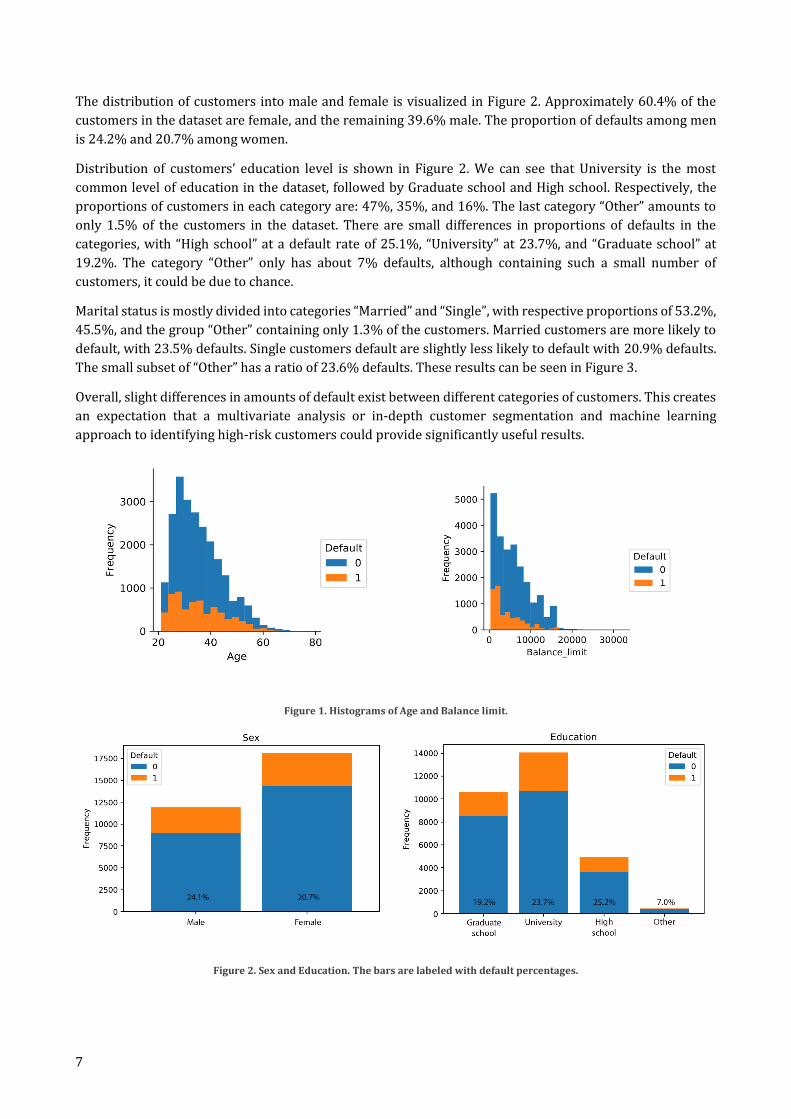
The median of 35 years, with a longer tail towards the right side, up to a maximum value of 79 years and a
minimum value of 21. The median and mean are quite close to each other, showing that the average age cuts
the distribution in half, as seen in Table 1. The mode of age is at 29 years, which can be seen as the highest
peak in Figure 1. On the basis of visual analysis, the difference in distributions of non-defaulting and
defaulting customers seems to be that there is a much more pronounced peak around 30 years among non-
defaulting customers. The distribution of age among defaulting customers seems to be more flat in
comparison. This indicates that older customers have a higher chance of default.
The distribution of balance limit has a large tail towards the higher values. The maximum value of balance
limit in the data is $32,300 but 75% of the values are less than $7,700. This effect can also be seen in Figure
1, which indicates it to be even more pronounced in the subset of customers that default. This points to
customers with low balance limit to possibly having a higher chance of default.
Table 1. Descriptive statistics of Age and Balance limit
Statistic Age Balance limit
Min 21 300
Max 79 32300
Mean 35.48 5400
Median 34 4500
Std. 9.21 4187
25% 28 1600
75% 41 7700
7
The distribution of customers into male and female is visualized in Figure 2. Approximately 60.4% of the
customers in the dataset are female, and the remaining 39.6% male. The proportion of defaults among men
is 24.2% and 20.7% among women.
Distribution of customers’ education level is shown in Figure 2. We can see that University is the most
common level of education in the dataset, followed by Graduate school and High school. Respectively, the
proportions of customers in each category are: 47%, 35%, and 16%. The last category “Other” amounts to
only 1.5% of the customers in the dataset. There are small differences in proportions of defaults in the
categories, with “High school” at a default rate of 25.1%, “University” at 23.7%, and “Graduate school” at
19.2%. The category “Other” only has about 7% defaults, although containing such a small number of
customers, it could be due to chance.
Marital status is mostly divided into categories “Married” and “Single”, with respective proportions of 53.2%,
45.5%, and the group “Other” containing only 1.3% of the customers. Married customers are more likely to
default, with 23.5% defaults. Single customers default are slightly less likely to default with 20.9% defaults.
The small subset of “Other” has a ratio of 23.6% defaults. These results can be seen in Figure 3.
Overall, slight differences in amounts of default exist between different categories of customers. This creates
an expectation that a multivariate analysis or in-depth customer segmentation and machine learning
approach to identifying high-risk customers could provide significantly useful results.
Figure 1. Histograms of Age and Balance limit.
Figure 2. Sex and Education. The bars are labeled with default percentages.

8
Figure 3. Marital status.
4.2.2. Distributions of age
To obtain more information that could be used in customer segmentation, age distributions of different
customer groups were visually examined using histograms of both default and non-default customers in
Figures 4-6.
Figure 4. shows the different levels of education and distributions of customers’ age among them. Graduate
school education seems to show a relatively higher peak around 30 years of age in the non-defaulting group
than in the defaulting group. This indicates that under 30 year old customers with a graduate school
education are slightly less likely to default than older customers with this level of education.
Another difference in default can be found in Figure 5, where the distribution of age among defaulting men
is much flatter than in their non-defaulting counterpart. The decline in number of customers starts from
about 30 years among the non-defaulting group, while the number of customers of different ages stays much
more constant from 25 to around 40 years. This indicates that likelihood of default among men grows with
age. For women, this effect is not as clearly visible.
Some differences can be found, but no clear guidelines can be made with this level of analysis of the
demographic variables. A more in-depth approach is required to meaningfully differentiate between low or
high risk customers. This analysis of distributions is however useful to understand some of the
characteristics of the data and to later describe the results of customer segmentation.
Figure 4. Education and Age.

9
Figure 5. Sex and Age.
Figure 6. Marital status and Age.
4.2.3. Correlation analysis
A correlation matrix of all variables in the dataset is shown in Figure 8. Most importantly, the only variable
with a notable correlation with default is payment status. The last month’s (September) payment status has
a Pearson correlation coefficient of 0.32 with default. The other months’ correlations are slightly lower. This
correlation is not surprising, since a customer with at least a month or more of delay in payments is naturally
more likely to not be able to pay their bills in the upcoming months.
The next highest correlation with default occurs with balance limit at -0.15, which itself is somewhat
negatively correlated with payment statuses. These measures indicate that customers with lower balance
limits have more delays in payments and are more likely to default. Figure 1 also supports this argument
since most defaulting customers have low balance limits, and payment status is correlated with default.
Balance limit also has a positive correlation coefficient of 0.14 with age, and a negative correlation of -0.23
with education. Age itself doesn’t seem to be correlated with default at all according to the Pearson
correlation coefficient. However, Figure 2 seems to show that the proportion of defaults among age groups
grows with age. Lower numerical values in education specify higher levels of education, and therefore the
negative correlation with balance limit can be understood as customers with a higher level of education
generally having credit limits. Bill amounts and payment amounts are also moderately positively correlated
with balance limit, but that is to be expected, since customers with higher credit are more likely to spend
more.
Correlation coefficients around 0.20-0.25 occur between bill amounts and payment statuses. This indicates
that customers with higher spending tend to have more delays in their payments.
Other demographic variables excluding balance limit show no correlation with default. Bill and payment
amounts have a very small correlation coefficient with default as well.

10
Figure 7. Correlation matrix of the entire dataset featuring all variables.
5. Research setup In order to study how the bank’s situation considering credit cards could be improved the whole problem
was divided into three subproblems. First we needed a financial model of the bank to simulate the bank’s
credit card business and to validate the effectiveness of our actions. After this we needed an actual model to
predict credit card defaults from our dataset. Lastly we also investigated what we could find out about the
bank’s customer base by clustering. By doing this we sought to provide a more interpretable solution for the
bank to balance out the “black box” nature of our default prediction model. In the clustering we aimed to find
financially significant customer segments for the bank and to see if there are some segments that are clearly
profitable or not which could then be included in our advice for the bank.

11
5.1. Financial model
The financial model was created in Python and used the information about the bank given to us by McKinsey
as well as the dataset of the customers. The financial model can calculate the monetary impact of an individual
customer based on their spending history and the knowledge of whether the customer defaults or not. This
calculation for an individual customer can the be repeated for each customer in our dataset to find out the
financial impact of a group of people which is useful when we want to investigate how for example, removing
risky customers effects the bank’s bottom line.
Kuutti bank has nearly 2 million customers with a credit card account out of whom nearly 750000 are
inactive but still pay annual fees for their credit cards. However our dataset only includes 30000 of these
people. This called for a method to extend our model to take into account the whole customer base instead
of just the dataset and also required that we assume the actions we take generalize for the whole customer
base. With this method, we are able to validate our results on the scale of the whole bank and not just a small
sample of 30000 customers.
The financial model was used in this project to validate both the default prediction algorithm and the
customer segmentation. In default prediction it was used to see how filtering out the high risk customers
predicted by the gradient boosting model would affect the bottom line of the bank and to see what would be
the optimal cut off point for denying people credit cards. In customer segmentation it was used to analyze
the monetary significance of the clusters i.e. which clusters are profitable and which clusters are not. This is
a bit more relevant measure for the preferability of the clusters since the plain default – no default division
does not necessarily tell the whole story how much money the bank earned or lost from that cluster.
5.2. Default prediction algorithm
For the default prediction algorithm we selected an ensemble machine learning algorithm called gradient
boosting which we could find readily from a machine learning library for Python. The algorithm was tuned
for our problem by running a parameter sweep that aimed to maximize the prediction accuracy in default.
We fitted two models for the data. One for all the features including the spending history and one for the
preliminary features age, sex, location, balance limit, education and marital status. The former was done as a
proof of concept that we are able to effectively predict defaults based on the data. The latter was the one that
actually had a useful application. This is because we are not able to remove people from the current customer
base since one can not aribtrarily terminate contracts but the thing that the bank can affect is whether they
accept someone as a customer or not. The filtering is extended to the whole customer base so it is taken into
account that the filtering would lower the total amount of customers that the bank has.
The models were then used to predict the default probability for each customer. Then high risk customers
were filtered out and the effect of the filtering was analyzed using the financial model as was previously
described. All the test were done so that the model is first trained on 80% of the data and then validated with
20% of the data.
5.3. Customer segmentation
The goal of customer segmentation is to provide a basis for differentiating between groups of customers
instead of single customers. This allows us to make predictions and measure the financial impact of actions
that affect large amounts of customers simultaneously and therefore creates a more generalized approach to
decision making. Communicating these results and actions, understanding them, and applying them is made
easier due to the simplified generalizations made with a customer segmentation approach. Instead of

12
providing a black-box model that outputs predictions for single customers, customer segmentation provides
useful generalizations of customer groups at the cost of accuracy.
To satisfy a useful customer segmentation, segments must contain customers similar to each other, while
varying from other segments such that a useful distinction can be made. A smaller number of customer
segments can provide a wide generalization that is easy to understand, but sacrifices accuracy due to more
variation within segments. On the other hand, a high number of segments can provide higher accuracy within
groups, but lose the ability to generalize, since segments are too highly specified.
To obtain a useful customer segmentation, in addition to taking into account the specificity and
generalizability of a segmentation, the segmentation is validated using the default prediction algorithm and
financial model to ensure accuracy and utility in terms of predicting default and improving the credit card
business of the bank. After obtaining a customer segmentation that satisfies these properties, it can be used
to justify and guide decisions such as to which customers bases should the bank further promote their credit
card business and with which customers should the bank attempt re-negotiating terms of contracts.
The segmentations will be made using unsupervised self-organizing maps, producing two-dimensional
representations of the customer base. The SOMs will be trained using a randomly sampled training set
containing 80% of the data. The training will only utilize six variables, which are Age, Balance limit, Marital
status, Education, Sex, and Location. Location is represented by a single variable, which contains the DBSCAN
cluster the customer is assigned to, similarly as it is in the default prediction algorithm for purposes of
predicting defaults of new clients. A large number of self-organizing maps with different parameters will be
trained to find suitable candidates for segmentation. After training the SOMs, the test set of customers is
assigned into their closest fitting nodes. Before describing the customer segments, a set of feasible maps are
tested and compared in terms of their accuracy and utility in categorizing default risk and financial impact.
Financial impact is measured using the financial model, which defines a net income value for each customer.
First, the test set is be used to validate the accuracy of predicting financial impact based on the default
prediction algorithms classifications. This approach allows us to study whether groups with higher predicted
risk actually produce more financial losses, and vice versa. In essence, this is to test how well gradient
boosting can be used to predict risk of groups of customers instead of single customers.
In addition to testing the ability to predict financial outcome through risk of default in the customer segments,
the segmentations’ accuracy in categorizing customers of similar risk level and financial impact together is
also tested. This is done by comparing amounts of true default and values of net income between the training
and test sets. This setup imitates a scenario where a customer segmentation is used to identify and categorize
new customers, and to approximate the customers’ risk level and net value to the bank. Comparing net
income values between the subsets of data measures how accurately customer segments represent net
income value, and comparing amounts of default measure how accurately the segments represent risk of
default.
These methods of validation also take into account the accuracy of mapping new customers into the self-
organizing maps, since inaccuracies will show up both in defaults and financial impact.
6. Results
6.1. Current financial situation of the bank
As it stands, the bank makes currently a profit of 22 million dollars from their credit card business. However

13
if we calculate the profit for just the people in the dataset the profit is approximately -600000 dollars. This
means that on average each customer in the dataset causes a loss of 20 dollars for the bank and the only thing
that keeps the credit card business profitable for the bank is indeed the inactive customers that pay the yearly
fee but otherwise do not use their card. Figure 8 shows the histogram of the profits per customer in the
dataset. We can see that the figure is heavily lopsided to the right and the most people have a financial impact
of -200 to 200 dollars the median being about 61 dollars.
However, what becomes detrimental to the bank is that there is no limit to how much they can lose but there
is effectively a limit on how much they can earn. This manifests itself in that the most profitable customer
brought just under 200 dollars to the bank whereas the largest individual loss was over 5000 dollars but the
histogram is cut off from the left since the data points get really sparse. In the dataset the bank has about
23000 profitable customers and about 7000 non profitable ones and the average loss is about 330 dollars
whereas the average gain is about 72 dollars. This means that even though there are many more profitable
customers, the higher average loss pulls the bottom line to the negative side.
Figure 8. Profit per customer.

14
6.2. Filtering customer base with gradient boosting
If we train the models for all the features and just the preliminary features we get the traditional
performance statistics seen in Tables 2 and 3. We can see that the model with all the features used in training
expectedly performs better on the traditional statistics. However the classification results are not that great
for either one of them. The model with all features manages to rightly predict 586 out of the total of 1333
defaulters where the model with just the preliminary ones manages to righly predict just 239 of them. Also
the accuracies are not that great considering that by just guessing “not default” you get about 80% accuracy.
However, this not the only way of validating our model. Since we have the financial model, we can check if
our models work even if the traditional metrics don’t seem too great. In addition to the classification, we can
get the predicted probabilities from the model which is basically how sure our model is that this person will
default. Using these predicted probabilities, we can do the classification manually by setting our own
classification limit and deeming people beyond that predicted probability risky customers and hence, not
preferable for the bank to have as customers. After removing risky customers from our customer base, we
can the use the financial model to see what kind of an effect that would have on our bank’s bottom line.
Confusion matrix for model with all features
Accuracy: 83.7%
Predicted class \ Actual class Not default Default
Not Default 4433 747
Default 234 586
Table 2. Confusion matrix, all features.
Confusion matrix for model with preliminary features
Accuracy: 78.6%
Predicted class \ Actual class Not default Default
Not Default 4479 1094
Default 188 239
Table 3. Confusion matrix, preliminary features.

15
If we run the model that includes all the features and see what kind of predicted probabilities they give to the
people we get the plots that can be seen in the Figure 9 In the top left corner is plotted the actual default
percentage against the predicted probability of default. For example out of people who have predicted
probability of 20% about 20% actually default. The figure also tells us that the higher the predicted
probability the higher the actual chance of defaulting which means that the model seems to be working. The
other three plots tell the absolute numbers of people in total population, defaulters and non defaulters. From
these we can see that the total population lowers rapidly as we approach higher predicted probabilities.
However, the absolute number of people who default remains pretty much the same even improving a bit.
This verifies what we saw in the upper left plot, the people with higher predicted probabilities actually have
higher risk for default which is good new considering usability of our model.
Now if we test how a filtering out higher risk customers affects the bottom line we get the plot seen in Figure
10 where profit is plotted as a function on the cut off point past which customers are removed.
Figure 9. Predicted probability of default and number of actual defaults.

16
Figure 10. Results of customer filtering.
From this figure, we can see that it is actually possible to improve bank’s bottom line using the predicted
probabilities of our model to filter out higher risk customers. From the figure, we can see that, for example,
if we filter out all the people who have higher than 20% predicted probability for default the total profit made
by the bank doubles which is a really good result. As we can see from the plots that are on the right in Figure
9 the amount of non defaulters increases rapidly in the beginning and most of them have a predicted
probability of 20% or less. This means that as we start increasing the cutoff point we are bringing in a lot of
non defaulting customers. However, the amount of defaulters was approximately evenly distributed. This
means that by including people with 20% or less predicted probability we actually get most of the non
defaulters but only about 20% of the defaulters and the figure shows that this is an effective way of increasing
the bottom line of the bank.
However the practical application of this model would be more difficult since eliminating people from
customer base along with their debt is not a viable option. This is more of a proof of concept that it is possible
to derive financially relevant information out of the dataset. More easily applicable knowledge would be if
we could filter out risky customers before they become customers. If we do the similar plot we did for the
previous model we get the plots seen in Figure 11.
We see that the results are not as nice as in the previous model. For example, the highest predicted
probabilities are lower than before which means that the model is not as sure about the peoples risk for
default. Despite this, we see similar features like the linear trend in the fraction of defaulters as the predicted
probability increases. Also, the quick rise and fall of the non defaulting population and the uniform
distribution of the defaulters are present. However, especially, the right tail of the non defaulting population
is pretty thick which means that many non defaulters also receive high predicted probabilities.
If we test how the predicted probabilities can be used to improve the bottom line we get the plot seen in
Figure 12.

17
Figure 11. Predicted probability of default and number of actual defaults.
Figure 12. Results of customer filtering.

18
This time the figure is not as clear as before and there are a few oddities like the dip to the negative side in
the beginning and the increase of the bottom line as we take in customers with predicted probabilities from
50% to 60% who should be the most risky customers of them all. However, we still see the similar result as
before that, generally speaking, if we filter out the higher risk customers our bottom line increases.
If we take a closer look at the two oddities in the figure by analysing the customers who have predicted
probability higher than 50% or 12% we get the histograms seen in Figure 13.
Figure 13. Histogram of customer profits.
From the images it is not immediately clear why the customers on the right are more profitable than the ones
on the left. The possible reasons could be that on the left there are more large defaults from people that the
model has deemed safe. This could be explained for example by that the balance limit feature correlates
positively with not defaulting. However when these people default the losses are generally high. It could be
that these people swing the average to the negative. On the left there are no that many high losses but there
are a few high gains so maybe they are able to make this segment profitable.
As it stands the average profit from people with predicted probability less than 12% is -22.6 and for people
with predicted probability of over 50% it is 4.2. This makes it clear that it would be profitable for the bank to
discard people with less than 12% predicted probability and include those with 50% or higher. However
these are more of an oddity or misperformance of our model and could be fixed with a better model so this
result is rather a feature of our model than a rule. It also need to be noted that here we are predicting with a
really limited knowledge of the customer. Wealthy people also default on their payments so it proposes a fair
challenge to get every single defaulter. One option to battle this could be to look into risk mitigation for the
bank rather than looking at just the predicted probability we could also include the balance limit in our
decision making. This would make it such that the bank has to be really sure on people who they are going to
give high balance limit. Other option would be to create a better model.
Despite this, it would still seem that it is possible to improve the bank’s bottom line with our model despite
the few flaws. If we select the people with predicted probability of less that 25% we still manage to double
our profit. In Figure 14 we can see the comparison between people with predicted probabilities of under and
over 25% i.e. the customer base and the people who are left out if we implement our model. We can clearly
see that on the right we have much more losses than on the left. Even though we still lose quite a bit of
profitable customers we manage to filter out a lot of the not profitables also. This verifies that filtering
according to our model would have a positive impact on the bank as well as on the profitability of the bank.

19
Figure 14. Histogram of customer profits.
6.3. Customer segmentation
6.3.1. Comparison of feasible segmentations
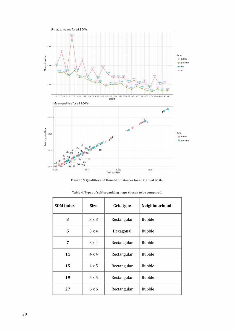
To find an optimal amount of customer segments, multiple self-organizing maps with different parameters
were trained. They were tested on two measures, the U-matrix distances and quality of representation. The
results are shown in Figure 15. Each SOM is referred to by an index, for example, ”SOM 3”. Quality represents
distance, which means lower quality equates to lower distances of objects to their respective nodes’ centers,
which is more desirable. U-matrix distance in Figure 15 measures the mean of that respective mapping’s
nodes’ distances to their neighbouring nodes. Higher values mean that nodes are farther away from each
other on average. Mean qualities of the maps were calculated both using the data in the training set, and data
in the test set that was first mapped into the grid. No significant difference in qualities was found between
the training and test set, which validates the accuracy of these maps. This can be seen from the linear shape
of the scatter plot.
Two different options were available for the neighbourhood function, gaussian and bubble. Maps using the
bubble neighbourhood function produced higher U-matrix distances, which may be simply a product of the
difference in metric instead of the capacity to represent difference in topology of the input space. Such
noticeable differences between the two neighbourhood functions could not be seen in qualities.
Maps with higher number of nodes tend to produce segmentations with high quality of representation (low
mean distance of objects to the center of their respective node). Similarly, a high number of nodes results in
lower distances between clusters. Both results are expected, since a higher resolution in in the grid will result
in a single node containing much more similar objects. At the same time, a high number of nodes means that
the distance between single neighbouring nodes gets smaller as well. The optimal grid size should be
something that is feasible to represent a customer segmentation, yet accurate and representative in terms of
the two distance measures that are compared.
According to these results, map numbers 3, 5, 7, 11, 15, 19, and 27 were chosen to be compared. The maps
parameters are shown in Table 4. The indices in the table correspond to the indices in Figure 16.
20
Figure 15. Qualities and U-matrix distances for all trained SOMs.
Table 4. Types of self-organizing maps chosen to be compared.
SOM index Size Grid type Neighbourhood
3 3 x 3 Rectangular Bubble
5 3 x 4 Hexagonal Bubble
7 3 x 4 Rectangular Bubble
11 4 x 4 Rectangular Bubble
15 4 x 5 Rectangular Bubble
19 5 x 5 Rectangular Bubble
27 6 x 6 Rectangular Bubble

21
6.3.2. Predicted default risk and financial impact
To measure and validate how well the gradient boosting algorithm can be used to predict risk and net value
of customer segments, the net income per customer for each cluster was calculated using the financial model.
The samples used here are from the test set. The results are shown in Figures 16-17. The bars are colored
based on proportion of samples classified as defaults by the gradient boosting. Darker colours indicate higher
predicted amount of defaults.
None of the segmentations show any consistency in terms of correlating higher predicted default ratio to
increased losses, or vice-versa. In any of the segmentations, multiple clusters with near to zero predicted
defaults can be seen producing higher losses than clusters with more defaults. If predicted default ratio could
be used to approximate net value of customer segments, the figures should show clusters with darker colors
(more defaults) consistently having higher losses.
Figure 16. Net income per customer in clusters of the tested segmentations.

22
Figure 17. Net income per customer in clusters of the tested segmentations.
6.3.3. Representation of net income
To measure how well the segmentations represent the net income of customers in that segment, the
difference of net income per customer in the test and training sets were calculated. Results are shown in
Figure 18. The maps with larger number of segments tend to have more variation in the differences.
Especially SOMs 19 and 27, which are 5x5 and 6x6 grids, have some clusters with large differences, even
though most differences are similar to other mappings, at around 0 to a 100 dollars. The smallest differences
across all segments can be seen in the smallest map, SOM number 3, which is a 3x3 rectangular grid. This is
most likely due to larger sample sizes in the clusters which means that single customers with high losses
don’t have as much weight in the normalized net income per customer. None of the differences exceed an
absolute value of a 100 dollars, and mostly stay between 0 to 40 dollars. Overall, these results show that none
of the segmentations are able to represent the average net income of customer groups consistently without
some errors.
These differences also shows that the values in Figures 16-17 can be very skewed and not entirely
representative of the actual net income of the clusters. For example, clusters 9 and 10 in SOM number 27, of
which the former creates positive net income measured in the test set, both have much higher estimated net
income than the training set shows.
6.3.4. Describing the segments
Due to the results seen in comparing net income differences in the test and training sets, and measuring
financial value estimation with predicted default, it is deemed that the larger mappings do not have enough
utility in either of these areas to justify their complexity. The best performer on average out of the smaller
mappings was the 3x3 rectangular grid (SOM 3). Even though in terms of default prediction, it did not seem
to perform any better than the other segmentations, the financial impact of the clusters can be considered
more trustworthy. Also due to having fewer segments, any description of the customer segments should be
more applicable and generalizable from the bank’s perspective. A closer inspection of the customer segments
in this mapping is done in order to understand the risk and net income better.
The self-organizing map’s codebook vectors are shown in Figure 19. It is important to note that the
numbering of units in these plots start from the bottom left and increase row by row to the right. For example,
the bottom row corresponds to segments 1, 2 and 3, and the second row to segments 4, 5, and 6, counting
from the left. The interpretation of the categorical variables’ values is explained in part (Describing the data).

23
These codebook vectors are of the same dimension as the original variables. Since the Kohonen R package
implementation of the distance metric used for categorical variables requires the variables to be binary, the
codebook vectors for these variables are shown being in the same dimension as the number of categories
and are plotted separately. For the location variable, this results in an 88-dimensional codebook vector due
to the number of different location clusters the variable represents. The location plot should be interpreted
as a histogram.
Figure 18. Difference of net income in test and training sets of data.

24
The codebook vectors offer a great way of understanding and describing what type of customers each
segment represents. Due to the way self-organizing maps work, the ideal customer for each segment would
be simply described by the codebook vectors values. Although, it should be remembered, that when a
customer is assigned to a segment, the segment which is closest to the customer will be chosen. So some
customers may vary from the center values represented by the codebook vectors. For example, using the
plots in Figure (codes), the proportion of customers in that segment having a certain education level can be
identified by comparing the sizes of the cones. For the continuous real-valued variables Age and Balance
limit, larger codebook vector values correspond to higher mean values of these variables in the segments.
Clear distinctions between customer groups can immediately be made based on the Sex, Education and
Marital status variables. Most customer segments represent only one type of customer in terms of education
level and sex. The marital status of customers in this segmentation varies more. Segments 1 and 4 can be
seen to consist of mostly married customers, while segment 5 has a roughly equal amount of single customers
and those with category “other”. Location data is very spread out across all of the segments, and all of the
codebook vector plots quite closely match the shape of the overall distribution of the location variable.
The results of calculating true default ratios and net incomes per customer for each segment, together with
the descriptions of a typical customer based on the codebook vectors and sample medians are summarized
in Figure 20. Location data was not included in this summary, since it is too spread out, and none of the
segments are simply characterized by location.
All of the segments still cause a negative income for the bank, due to high numbers of default. Comparing the
risk of customer segments measured by default ratio does not directly imply similar differences in net
income. For example, customer segment number 9 (top right corner) in Figure 20 causes a mean loss of 205
dollars. However, customer segment 6 below 9, with a default ratio of 21%, causes the least loss at a 100
dollars.
Figure 19. Codebook vectors of the 3x3 rectangular SOM.

25
Figure 20. Summary of customer segmentation using the 3x3 rectangular SOM.
7. Conclusions The results of customer segmentation show that neither directly measuring or using predicted proportion of
defaults of a customer group to predict net income is accurate. This is most likely due to multiple reasons.
One of them being the limitations in accuracy of any machine learning algorithm caused by the small number
of variables. Another reason is most likely the lack of specificity in customer segments, mixing up actual high
risk customers with those of low risk. Comparing net incomes in the training set and test set also showed
large variation. This is most likely due to the high losses that a single customer can produce by defaulting
with high amounts of debt. Much of the variation in the data could not be represented, since customer
segmentation was only done using the demographic variables. Considering all of the results in customer
segmentation, the segments are most likely not sufficiently homogeneous representations of a customer type
to predict risk or financial value accurately. Further analysis should be done in order to fully justify and
support business decisions based on the customer segmentation in this study. Perhaps using the
segmentations created by the self-organizing maps as templates for customer groups to guide more in depth
analysis of certain types of customers instead of calculating averages over the entire mapped population
could give better results.
When it comes to default prediction, we have a model that is able to predict the defaults of customers with
high enough certainty that the bank can utilize it in their functions. Assuming that the banks continues to
receive customers that are represented in our dataset we could implement our model in the banks
preliminary screening process and it would bring financial gain to the bank. However, our solution is not
viable to be used as a standalone system in its current form since it only considers part of the banks actions.
Many factors that were not covered in this case study should be taken into consideration when taking any
business action. For example young people could be preferable for the bank since they stay longer as a
customer so it could be in banks interest to favor having them as a customer even if our model would suggest

26
otherwise. Single customers should not be discriminated against especially based on the customer
segmentation which relies on calculating averages over a group. A single customer defaulting with high debt
can result in much higher losses than might be anticipated simply based on averages. Similarly, the analysis
does not go in-depth enough to justify assuming that the variables used in this study could explain or predict
how reliable the customers are on the long run, especially considering that the data was collected during a
debt crisis.
8. Self assessment
How was the project executed? We started the project by comparing the results of classification accuracy of different machine learning
algorithms such as logistic regression, decision trees, and discriminant analysis. After that, the financial
model was built. Then, we tried other machine learning techniques like gradient boosting, which was the
main prediction method used. For customer segmentation, many different clustering methods were tested.
Even manually choosing customer types was considered, but proved to be too ineffective.
In the beginning of the project, a decision tree was used for segmenting the customers, but then we decided
to do the entire task of customer segmentation independent of any predictions or knowledge of defaults. Self-
organizing maps were used to perform an unsupervised mapping that was easy to interpret and tweak in
terms of number of segments.
Meetings with McKinsey mostly consisted on reporting our progress and discussing ideas on how to move
forward. McKinsey gave us plenty of freedom on how to approach the problem, which had its positive and
negative sides.
What was the real amount of effort? The real amount of effort is rather hard to estimate, since the course has taken so long. With steady pace the
course would have taken about 6 hours per week of work but in reality, the work focused around the
presentations. It was nice that there was so many “check points” since it made pacing out work much easier.
Of course, the projects are pretty hard to balance when it comes to workload since the subjects differ so much.
The amount of effort is also very dependent on how the scope and objective of the project is defined. In
hindsight, a lot of the time effort could have been better spent if we had a better grasp of what we are trying
to achieve as a group of individuals and in terms of what exactly our client bank needs.
In what regard was the project successful? The project was successful in the sense that many of the tools and methods we used were more or less new
to the group members, which was a great opportunity to learn them. Also, our project differed quite a bit
from the other subjects since other problems were more or less real business problems that the companies
faced whereas our subject was more kind of a case study. This has its ups and downs. Compared to other
subject, ours was “safe” in the way that we knew we could get actual results and it was always pretty clear
what could be done. However our subject lacks the excitement of doing something no-one has ever done
before. Technically, we were at least successful in creating a default prediction algorithm, a customer
segmentation and testing their combination.
In what regard was it less so? In terms of objectives set by McKinsey, the business aspect of coming up with a real plan for default mitigation
was not successful. At least partially for the reason that there was no real client with whom we could have
kept discussing our goals, the end product that we were planning to make was never properly defined. For
example, the financial figures that we used to model the bank’s finances were summarized in one or two
slides. A more in depth understanding of the bank’s business operations and interaction with customers
could have helped us to shape the project. McKinsey gave us freedom to create any kind of a financial plan

27
we deemed fit, but work effort wasn’t properly guided to achieve this goal. This is partially due to the internal
management and group dynamics during the project. The group should have made it a task itself to define
what is required from the perspective of the client bank and what needs to be done in order to achieve that.
What could have been done better, in hindsight? The freedom of an open subject is a gift and a curse. I think we did a lot of things that did not directly benefit
our project but seemed cool and interesting to take a look at. This leads to a quite a bit branching of our
project. It would have probably been beneficial to have a one clear goal where we want to get to and plan our
doings such that they directly benefit our goal. This way we probably would have achieved a much more
coherent result. The first submission, project plan, was a good thing and the project would have probably
been even more disorganized without it. However, even though the branching did not benefit our end result,
it was still probably the most educational part of the course. We got to learn about numerous new things and
the freedom given by the course and the subject made it possible to try all sorts of things to see if they work.

28
References
[1] I-Cheng Yeh and Che-Hui Lien. (2009) “The Comparisons of Data Mining Techniques for the Predictive
Accuracy of Probability of Default of Credit Card Clients”, Expert Systems with Applications, 36, pp. 2473-2480.
[2] Federal Reserve. (2018) “Charge-Off and Delinquency Rates on Loans and Leases at Commercial Banks”.
Available at: https://www.federalreserve.gov/releases/chargeoff/default.htm
[3] Federal Reserve. (2018) “Consumer Credit Historical Data”, Federal Reserve G-19. [Online]. Available at:
https://www.federalreserve.gov/releases/g19/HIST/default.htm
[4] Federal Reserve. (2017) “Report to the Congress on the Profitability of Credit Card Operations of
Depository Institutions”. Available at: https://www.federalreserve.gov/publications/2017-report-to-
congress-profitability-credit-card-operations-depository-institutions.htm
[5] Taiwo Oladipupo Ayodele. (2010) “Types of Machine Learning Algorithms”, New Advances In Machine
Learning, Yagang Zhang (Ed.), Intech.
[6] Martin Ester, Hans-Peter Kriegel, Jiirg Sander, Xiaowei Xu. (1996) "Density-Based Algorithm for
Discovering Clusters in Large Spatial Databases with Noise", in KDD'96 Proceedings of the Second
International Conference on Knowledge Discovery and Data Mining, AAAI Press, Portland, Oregon, pp. 226-
231
[7] Jerome H. Friedman. (2002) "Stochastic Gradient Boosting", Computational Statistics & Data Analysis, 38,
Issue 4, pp. 367-378.
[8] Aarshay Jain, (2016) Complete Guide to Parameter Tuning in Gradient Boosting (GBM) in Python.
Available at: https://www.analyticsvidhya.com/blog/2016/02/complete-guide-parameter-tuning-
gradient-boosting-gbm-python/
[9] Teuvo Kohonen and Timo Honkela. (2007) “Kohonen network”, Scholarpedia, 2(1):1568.
[10] R. Wehrens and L.M.C. Buydens. (2007) Self- and Super-organising Maps in R: the kohonen package J.
Stat. Softw., 21(5). Available at: http://www.jstatsoft.org/v21/i05