Predicting Ground Motion from Earthquakes

“If we know where a major earthquake is likely to occur, how large will the ground

motion be at a particular site?”

Art McGarr

Summary of Strong Ground Motion from Earthquakes

• Measured using PGA, PGV, pseudo-spectral acceleration or velocity PSA or PSV, and intensity.

• Increases with magnitude.

• Enhanced in direction of rupture propagation (directivity).

• Generally decreases with epicentral distance.

• Low-velocity soil site gives much higher ground motion than rock site. Vs30 is a good predictor of site response.

Call them “Ground-Motion Prediction Equations”

• “Attenuation Equations” is a poor term– They describe the INCREASE of amplitude

with magnitude at a given distance– They describe the CHANGE of amplitude

with distance for a given magnitude (usually, but not necessarily, a DECREASE of amplitude with increasing distance).

Ground Motion Prediction Equations

• Empirical regressions of recorded data• Estimate ground shaking parameter (peak ground

acceleration, peak velocity, spectral acceleration or velocity response) as a function of

(1) magnitude

(2) distance

(3) site• May consider fault type (strike-slip, normal,

reverse)

Developing EquationsDeveloping Equations• When have data (rare for most of the world):

– Regression analysis of observed data

• When adequate data are lacking: – Regression analysis of simulated data (making use of motions

from smaller events if available to constrain distance dependence of motions).

– Hybrid methods, capturing complex source effects from observed data and modifying for regional differences.

Observed data adequate for regression exceptclose to large ‘quakes

Observed data not adequate for regression, use simulated data

1 10 100 1000

5

6

7

8

Mom

ent

Mag

nitu

de

Used by BJF93 for pga

Western North America

1 10 100 1000

5

6

7

8

Distance (km)

Mom

ent

Mag

nitu

de

AccelerographsSeismographic Stations

Eastern North America

File

:D:\

me

tu_

03

\re

gre

ss\m

_d

_w

na

_e

na

_p

ga

.dra

w;D

ate

:20

05

-04

-20

;Tim

e:

20

:29

:49

What to use for the Predictor Variables?

• Moment magnitude

• Some distance measure that helps account for the extended fault rupture surface (remember that the functional form is motivated by a point source, yet the equations are used for non-point sources)

• Site terms

• Maybe style of faulting

How does the motion depend on magnitude?

• Source scaling theory predicts a general increase with magnitude for a fixed distance, with more sensitivity to magnitude for long periods and possible nonlinear dependence on magnitude

• Of the many magnitude scales, which is the most useful for ground motion prediction?

Moment Magnitude

• Best single measure of overall size of an earthquake

• Can be determined from ground deformation or seismic waves

• Can be estimated from paleoseismological studies

• Can be related to slip rates on faults

10-1 1 101 1020.01

0.1

1.0

10

100

Frequency (Hz)

Fou

rier

acce

lera

tion

spec

trum

(cm

/sec

)

M 5 to 8 in steps of 0.5

R = 20 km

File

:C

:\m

etu_

03\r

egre

ss\f

as_r

ange

_of_

m.d

raw

;D

ate:

2003

-09-

02;

Tim

e:21

:23:

19

4 5 6 7 80.1

1

10

100

1000

M

PS

A(c

m/s

ec2)

R = 20 km

T = 0.20 sec

T = 1.0 sec T = 2.0 sec

File

:C:\m

etu

_0

3\r

eg

ress

\psa

_vs

_m

_t0

p2

_1

p0

_2

p0

.dra

w;D

ate

:20

05

-05

-05

;Tim

e:

14

:48

:34

How does the motion depend on distance?

• Generally, it will decrease (attenuate) with distance

• But wave propagation in a layered earth predicts more complicated behavior (e.g., increase at some distances due to critical angle reflections (“Moho-bounce”)

• Equations assume average over various crustal structures

• Many different measures of distance

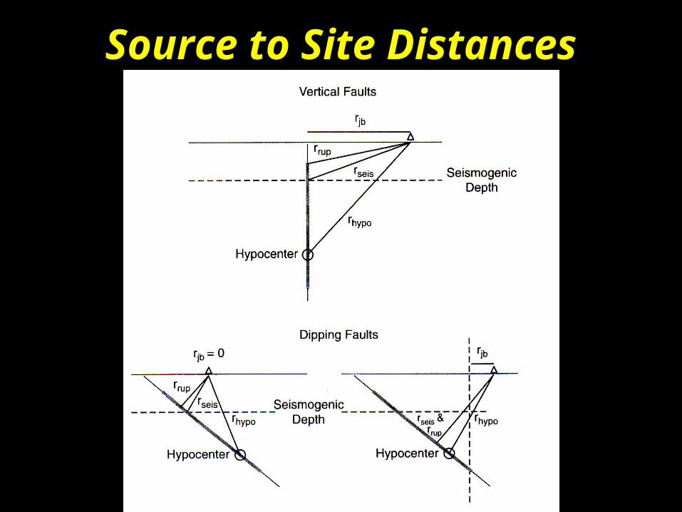
Source to Site Distances

Path effects• Wave types

– Body (P, S)– Surface (Love, Rayleigh)

• Amplitude changes due to wave propagation– Geometrical spreading (1/r in uniform media, more rapid decay for

velocity increasing with depth)– Critical angle reflections– Waveguide effects

• Amplitude changes due to intrinsic (conversion to heat) and scattering attenuation [exp(-kr)]

CharacteristicsCharacteristics of Data

• Change of amplitude with distance for fixed magnitude

• Change of amplitude with magnitude after removing distance dependence

• Site dependence

• Scatter

"It is an easy matter to select two stations within 1,000 feet of each other where the average range of horizontal motion at the one station shall be five times, and even ten times, greater than it is at the other”

John Milne, (1898, Seismology)

Spatial VariabilitySpatial Variability

What functional form to use?

• Motivated by waves propagating from a point source

• Add more terms to capture effects not included in simple functional form

People have known for a long time thatPeople have known for a long time thatmotions on soil are greater than on rockmotions on soil are greater than on rock

• e.g., Daniel Drake (1815) on the 1811-1812 New Madrid sequence:

•

– "The convulsion was greater along the Mississippi, as well as along the Ohio, than in the uplands. The strata in both valleys are loose. The more tenacious layers of clay and loam spread over the adjoining hills … suffered but little derangement."

Site Classifications for Use WithSite Classifications for Use WithGround-Motion Prediction EquationsGround-Motion Prediction Equations

• Rock = less than 5m soil over “granite”, “limestone”, etc.• Soil= everything else

2. NEHRP Site Classes

3. Continuous Variable (V30)

1. Rock/Soil

620 m/s = typical rock

310 m/s = typical soil

Empirically-based Prediction Equations: Results and

Comparisons

1 10 100 1000

5

6

7

8

Distance (km)

Mom

ent

Mag

nitu

de

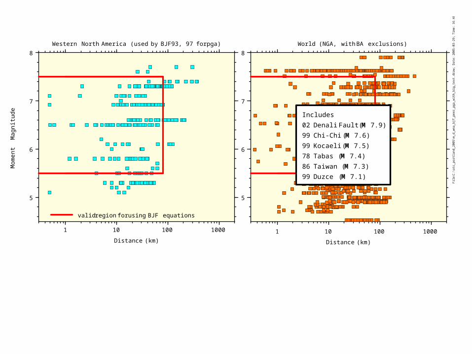
valid region for using BJF equations

Western North America (used by BJF93, 97 for pga)

1 10 100 1000

5

6

7

8

Distance (km)

World (NGA, with BA exclusions)

File

:C

:\atc

_por

tland

_200

5\m

_d_w

na_b

jf_pe

er_p

ga_w

ith_b

ig_t

ext.d

raw

;D

ate:

2005

-03-

29;

Tim

e:16

:48:

28

Includes02 Denali Fault (M 7.9)99 Chi-Chi (M 7.6)99 Kocaeli (M 7.5)78 Tabas (M 7.4)86 Taiwan (M 7.3)99 Duzce (M 7.1)

10-1 1 101 102

10-1

1

Distance (km)P

ea

kA

cce

lera

tion

(g)

NEHRP Class DM 5.5

M 6.5

M 7.5

1 101 102

1

101

102

Distance (km)

5%

da

mp

ed

PS

V(c

m/s

)

NEHRP Class DM 5.5

M 6.5

M 7.5

T = 0.3 sec

1 101 102

101

102

Distance (km)

5%

da

mp

ed

PS

V(c

m/s

)

NEHRP Class DM 5.5

M 6.5

M 7.5

T = 1.0 sec

File

:C

:\m

etu

_0

3\r

eg

ress

\PA

PV

VS

D.d

raw

;Da

te:2

00

3-0

9-0

3;T

ime

:1

6:3

2:4

5

A&S, sS, Vs=600

0.001

0.01

0.1

1

1 10 100 1000

PG

A (

g)

Rupture Distance (km)

5

5.5

6

6.5

7

7.5

M8, AR=2

M8, AR=4

M8, AR=8

M8, AR>15

0 20 40 60 80 1000

0.2

0.4

0.6

0.8

1

1.2

djb

peak

horiz

onta

lac

cele

ratio

n(g

)

BJF93, random, NEHRP D, M=7.0shaded: median/10 , median*10

0.1 1 10 100

0.1

0.2

0.3

1

djb

BJF93, random, NEHRP D, M=7.0shaded: median/10 , median*10

File

:C

:\m

etu_

03\r

egre

ss\p

gam

7vsd

.dra

w;

Dat

e:20

03-0

9-05

;Ti

me:

12:3

6:40

Strong-motion Recordings from the 1994 M6.7 Northridge Earthquake

Ground-Motion Prediction EquationsGround-Motion Prediction Equations

Gives mean and standard deviation of response-spectrum ordinate (at a particular frequency) as a function of magnitude distance, site conditions, and perhaps other variables.

10-1 1 101 102

0.01

0.1

1.0

Shortest Horiz. Dist. to Map View of Rupture Surface (km)

La

rge

rH

ori

zon

talP

ea

kA

cce

l(g

)

1992 Landers, M = 7.31994 NR, M=6.7 (reduced by RS-->SS factor)Boore et al., Strike Slip, M = 7.3, NEHRP Class D_+

File

:D

:\m

etu

_0

3\r

eg

res

s\B

JF

LN

DN

R.d

raw

;Da

te:2

00

5-0

4-2

0;T

ime

:2

0:2

5:2

6

0.1 0.2 1 21

101

102

Period (sec)

Pse

udo

Rel

ativ

eV

eloc

ity(c

m/s

)

Mechanism: strike slipMechanism: reverse slip

SoilM = 7.5

D = 0 km

D = 10 km

D = 20 km

D = 40 km

D = 80 km

File

:C

:\m

etu

_0

3\r

eg

res

s\F

IG8

_s

rl_

fau

lt_

typ

e.d

raw

;D

ate

:20

03

-09

-03

;Tim

e:

18

:47

:06

0.1 1 10 100

10

100

1000

10000

Rjb (set values less than 0.1 to 0.1 km)

PS

A(c

m/s

ec2)

Chi-Chi (M 7.6)Loma Prieta (M 6.9)Northridge (M 6.7)

T = 0.1 sec

0.1 1 10 100

Rjb (set values less than 0.1 to 0.1 km)

Chi-Chi (M 7.6)Loma Prieta (M 6.9)Northridge (M 6.7)

T = 2 sec

File

:C

:\p

ee

r_n

ga

\te

am

x\rs

_t0

p1

_t2

p0

_ch

i_ch

i_lp

89

_n

r94

.dra

w;D

ate

:20

05

-05

-03

;Tim

e:

12

:07

:50

Chi-Chi data are low at short periods(note also scatter, distance dependence)

Illustrating distance and magnitude dependence

An Extreme Site Effect -1985 M8.1 Michoacan

Earthquake

Site Response: 1985 Michoacan, Mexico Earthquake

Mexico City ・ 350 km from earthquake epicenter ・ 9000 deaths ・ collapse of 371 high rise structures, especially 10-14 story

buildings

Anderson et al., 1986

Strong-motion Records from Mexico City

old lake bed

hard rock hills

Mexico City Acceleration Response Spectrum

Recorded data

Expected ground motions

Resonance Period of10 to 14 story buildings

PGA generally a poor measure of ground-motion intensity. All of these time series have the same PGA:

0 50 100 150-0.2

-0.1

0

0.1

0.2

Acc

eler

atio

n(g

) Peru, 5 Jan 1974, Transverse Comp., Zarate

M = 6.6, rhyp = 118 km

0 50 100 150-0.2

-0.1

0

0.1

0.2

Acc

eler

atio

n(g

) Montenegro, 15 April 1979, NS Component, Ulcinj

M = 6.9, rhyp = 29 km

0 50 100 150-0.2

-0.1

0

0.1

0.2A

ccel

erat

ion

(g) Mexico, 19 Sept. 1985, EW Component, SCT1

M = 8.0, rhyp = 399 km

0 50 100 150-0.2

-0.1

0

0.1

0.2

Time (sec)

Acc

eler

atio

n(g

) Romania, 4 March 1977 EW Component, INCERC-1M = 7.5, rhyp = 183 km

File

:D

:\e

nc

yc

lop

ed

ia_

bo

mm

er\

ac

ce

l_s

am

e_

pg

a.d

raw

;Da

te:2

00

5-0

4-2

0;T

ime

:1

9:4

4:3

3

0.1 1 1010-5

10-4

0.001

0.01

0.1

1

Period (sec)

Peru (M=6.6,rhyp=118km)

Montenegro (M=6.9,rhyp=29km)

Mexico (M=8.0,rhyp=399km)

Romania (M=7.5,rhyp=183km)

File

:D

:\e

ncy

clo

pe

dia

_b

om

me

r\p

sa_

sam

e_

pg

a.d

raw

;D

ate

:2

00

5-0

4-2

0;T

ime

:1

9:3

4:1

6

0 2 4 6 8 100

0.2

0.4

0.6

0.8

1

Period (sec)

5%-D

ampe

d,P

seud

o-A

bsol

ute

Acc

eler

atio

n(g

)

Peru (M=6.6,rhyp=118km)

Montenegro (M=6.9,rhyp=29km)

Mexico (M=8.0,rhyp=399km)

Romania (M=7.5,rhyp=183km)

But the response spectra (and consequences for structures) are quite different (lin-lin and log-log plots to emphasize different periods of motion):

File

:C

:\m

etu

_0

3\r

eg

res

s\p

sa

_b

jf_m

55

_m

75

_c

las

s_

b_

c_

d.d

raw

;Da

te:2

00

3-0

9-0

6;T

ime

:1

2:1

6:4

9

0 0.5 1 1.5 2 2.5

0

500

1000

1500

Period (sec)

5%-D

ampe

d,P

seud

o-A

bsol

ute

Acc

eler

atio

n(c

m/s

ec2)

M=7.5, NEHRP classes B, C, DM=5.5, NEHRP classes B, C, D

Boore, Joyner, and Fumal (1997); rjb = 10 km

BC

D

0.1 0.2 0.3 1 2

10

20

100

200

1000

2000

Period (sec)

M=7.5, NEHRP classes B, C, DM=5.5, NEHRP classes B, C, D

Perception of results depends on type of plot (linear, log)

Ground Motion Prediction• Intended to predict PGA, PGV, or spectral response at

periods of engineering interest• logY=a1+a2(M-Mr1)+a3(M-Mr2)+a4R+a5LogR+site+a6F• Coefficients ai are determined by regression fits to ground

motion data sets.• Ground motion generally increases with M and decreases

with R• Site term mostly depends on near-surface shear-wave

speed, usually expressed as Vs30• Site effects sometimes dominate • Response spectra much more useful than PGA for

predicting structural damage