Prediction of Small-Scale Cavitation in a High SpeedFlow Over an Open Cavity Using Large Eddy

Simulation

Ehsan ShamsSourabh V. Apte∗

Computational Flow Physics LaboratorySchool of Mechanical Industrial and Manufacturing EngineeringOregon State University, 204 Rogers Hall, Corvallis, OR 97331

AbstractLarge-eddy simulation of flow over an open cavity corresponding to the experimental

setup of Liu and Katz [1] is performed. The filtered, incompressible Navier-Stokes equa-tions are solved using a co-located grid finite-volume solver with the dynamic Smagorin-sky model for subgrid scale closure. The computational grid consists of around sevenmillion grid points with three million points clustered around the shear layer and theboundary-layer over the leading edge is resolved. The only input from the experimentaldata is the mean velocity profile at the inlet condition. The mean flow is superimposedwith turbulent velocity fluctuations generated by solving a forced periodic duct flow atfree-stream Reynolds number. The flow statistics, including mean and rms velocityfields and pressure coefficients, are compared with the experimental data to show rea-sonable agreement. The dynamic interactions between traveling vortices in the shearlayer and the trailing edge affect the value and location of the pressure minima. Cavita-tion inception is investigated using two approaches: (i) a discrete bubble model whereinthe bubble dynamics is computed by solving the Rayleigh-Plesset and the bubble motionequations using an adaptive time-stepping procedure, and (ii) a scalar transport modelfor the liquid volume fraction with source and sink terms for phase change. LES to-gether with the cavitation models predict that inception occurs near the trailing edgesimilar to that observed in the experiments. The bubble transport model captures thesubgrid dynamics of the vapor better, whereas the scalar model captures the large-scalefeatures more accurately. A hybrid approach combining the bubble model with the scalartransport is needed to capture the broad range of scales observed in cavitation.

1 INTRODUCTION

The problem of cavitation has been widely studied owing to its influence on structural vibra-tions, noise production, erosion of propulsor blades, among others [2]. To devise strategies to

∗Address all correspondence to this author. Email: sva@engr.orst.edu

1

avoid cavitation, it is necessary to predict its inception in unsteady turbulent flows. Rood [3]provides a review of different mechanisms of cavitation inception emphasizing that cavita-tion inception and turbulence are inseparable in many applications. Therefore, predictivenumerical approaches (such as large-eddy simulations) for turbulent flows in complex flowconfigurations are necessary to accurately capture the inception process. However, modelingsmall-scale cavitation, cavitation inception and its unsteady evolution in engineering geome-tries is a challenging task. Liu and Katz [1] (henceforth referred to as LK2008) designeda well quantified experiment on high speed flow over an open cavity which can be usedfor detailed validation of the numerical approach in predicting cavitating flows in complexgeometries as well as development and testing of subgrid scale models.

The cavitation number [σi = (Pref − Pv)/(0.5ρ`U2∞)], where Pv is the vapor pressure, ρ`

is the liquid density, U∞ is reference velocity, and Pref is reference pressure value at whichcavitation occurs, has typically been used to predict cavitation inception. If we assume thatinception occurs when the pressure drops below vapor pressure, then a critical coefficientof pressure can be defined as Cp,min = (Pmin − Pref )/(0.5ρU

2∞) = −σi, where Pmin is the

minimum pressure within the domain. In turbulent flows, the location and the value ofminimum pressure can change dramatically, and thus can affect the inception process. Forhigh-speed flow over an open cavity, LK2008 showed that cavitation inception occurs abovethe trailing edge. However, they also observed a periodic variation in the amount of cavitationdue to variations in pressure fields induced by the turbulent shear flow above the cavity.

Several numerical studies on cavitation inception have been performed for gaseous cav-itation (i.e. growth of air micro-bubbles without significant transfer of mass from liquid tothe bubble) [4, 5, 6, 7, 8, 9, 10, 11]. A majority of these studies used Reynolds-averagedNavier Stokes (RANS) models to predict cavitation inception. Recently, large-eddy sim-ulation (LES) has also been used to study cavitation inception in a flow over a squarecylinder [12]. A simple algebraic criterion for inception was developed based on stability ofbubble nuclei to show good predictive capability of the LES methodology.

In the present work, LES of turbulent shear flow developing past an open cavity isperformed to first investigate the predictive capability of LES with the dynamic Smagorinskymodel [13]. Distribution of the coefficient of pressure (mean and rms) is used to identifycavitation inception regions over the trailing edge of the cavity and inside the shear layer.Cavitation inception is also studied by considering two types of models: (i) a discrete-bubblemodel (DBM) for gaseous cavitation based on the bubble-dynamics represented by Rayleigh-Plesset equation, and (ii) a scalar-transport model typically used for vaporous cavitation(involving phase change) [14, 15]. As the first step, the effect of the gaseous or vapor bubbledynamics on the fluid are neglected; that is the bubbles are assumed not to significantlyaffect the flow.

In the following sections, a brief overview of the mathematical formulation for the twomodels is presented. The discrete bubble model, involves computation and tracking of largenumber of bubble nuclei and can be expensive. An adaptive time-stepping scheme is devel-oped and validated for efficient computation. These models are coupled with an LES solverand the results obtained are discussed in detail.

2

2 MATHEMATICAL FORMULATION

In this section, the mathematical formulation for the single-phase LES and the two-phaseflow models are described. The three-dimensional, incompressible, filtered Navier-Stokesequations are written as

∂ui∂xi

= 0 (1)

∂ui∂t

+∂uiuj∂xj

= − 1

ρ`

∂P `

∂xi+ ν`

∂2ui∂xjxj

−∂τ rij∂xj

, (2)

where τ rij denotes the anisotropic part of the subgrid-scale stress tensor, uiuj −uiuj, and theoverbar indicates filtered variables, ν` is the kinematic viscosity and ρ` is the density of theliquid. The dynamic Smagorinsky model [13] is modified for unstructured grids and used forτ rij. In Smagorinsky model, it is assumed that

qrij = −2C∆2|S|Sij, (3)

where qrij is the aniostropic part of the subgrid scale stress (τ rij = uiuj − uiuj), Sij is the

filtered strain-rate tensor, and ∆ is the filter width. Using least-squares approach for thedynamic procedure to compute the coefficient C yields,

C∆2

= −1

2

MijLijMklMkl

, (4)

whereLij = uiuj − uiuj, (5)

and

Mij =(

∆/∆)2

|S|Sij − |S|Sij. (6)

Here the test-filter is denoted by the symbol ( ), and the ratio of the test to grid filter(

∆/∆)

is commonly assumed to be 2. The filter width is defined as V1/3cv , where Vcv is the volume of

the control volume and a top-hat test-filter is used based on the neighboring control volumes.

2.1 Discrete Bubble Model

The discrete-bubble model is based on an Eulerian-Lagrangian approach. A continuum de-scription is used for the liquid phase with discrete Lagrangian tracking of the bubbles. Thebubbles are usually treated as spherical point-particles with models for fluid-bubble interac-tion forces and bubble-bubble interactions. The bubble growth and collapse is modeled usingthe Rayleigh-Plesset equation [16, 6, 11]. Typically, in this type of discrete bubble model,small-size nuclei are assumed trapped inside the fluid. Existing nuclei or microbubbles maycontain gas or vapor or a mixture of both. These nuclei may undergo rapid changes in sizedue to local pressure variations and can be used an as indicator of cavitation inception. Thegrowth and collapse of bubbles can affect the fluid flow through momentum coupling as well

3

as through changes in bubble volume. In the present work we focus on cavitation inception,and do not consider the bubble-fluid coupling as well as effects of local void fraction varia-tions [17]. The bubbles are thus simply tracked by solving the following equations for thebubble position (xb), velocity (ub), and radius (Rb):

d

dt(xb) = ub (7)

mbd

dt(ub) =

∑Fb (8)

ρ`

[Rbd2Rb

dt2+

3

2

(dRb

dt

)2]

= Pb − P out −2σ

Rb

− 4µ`Rb

dRb

dt(9)

where mb is the mass,∑

Fb is the total force acting on the bubble, Pb and P out are thepressures inside and outside of the bubble, respectively, σ is the surface tension coefficient,and µ` and ρ` are the liquid viscosity and density, respectively. To estimate Pb, it is typicallyassumed that the bubble contains some contaminant gas which expands or contracts accord-ing to adiabatic or isothermal processes [18, 19]. The pressure inside the bubble consists ofcontribution from the gas pressure (Pg) and the vapor pressure (Pv). The net bubble-pressureis computed as:

Pb = Pv + Pg = Pv + Pg,0

(Rb,0

Rb

)3η

, (10)

where Pg,0 and Rb,0 are the reference partial pressure and bubble radius, respectively. Forisothermal bubble expansion η = 1 whereas for an adiabatic expansion, η = cp/cv (the ratioof specific heats of the gas at constant pressure and volume). The outside pressure P out

is taken as the pressure field interpolated to the bubble center location. Chahine and co-workers [6, 5] have shown that the bubble surface-averaged pressure (SAP) provides a betterrepresentation of the outside pressure. The net force acting on each individual bubble isgiven as [4]: ∑

Fb = FG + FP + FD + FL + FAM + Fcoll + FRb(11)

where FG = (ρb − ρ`)Vbg is the gravitational force, FP = −Vb∇P is the pressure force dueto external pressure gradients, FD = −1

2CDρ`πR

2b |ub − u`|(ub − u`) is the drag force, FL =

−CLρ`Vb(ub−u`)×∇×u` is the lift force, FAM = −12ρ`Vb

(Dub

Dt− Du`

Dt

)is the added mass force,

and Fcoll is the inter-bubble or bubble-wall collision forces. The force FRb= −4ρ`πR

2b(ub −

u`)dRb

dtrepresents momentum transfer due to variations in bubble size. Here, Vb and Rb are

the bubble volume and radius, the subscripts ‘b’ and ‘`’ correspond to the bubble and thefluid, respectively. Inter-bubble and bubble-wall interaction forces are computed using thestandard collision models typically used in the discrete element method [20]. Several differentmodels for the drag (CD) and lift (CL) coefficients have been proposed that account for bubbledeformation and variations in bubble Reynolds numbers (Reb = ρ`|ub − u`|2Rb/µ`) [21]. Thedrag coefficient used in this study is given as:

CD =24

Reb(1 + 0.15Re0.687

b ).

The bubble dynamics is mainly governed by the outside pressure changes. In low pressureregions, the bubble size can vary rapidly and the Rayleigh-Plesset equations become very

4

stiff. An adaptive time stepping algorithm is used to efficiently solve for several bubbletrajectories and still keep the overall computational time small [17, 22].

2.2 Scalar Transport Model

Eulerian-Eulerian two-phase models are also commonly employed in cavitation studies [14,23, 15, 24]. These models usually are important for large-scale, vaporous-cavitation where alarge region of the fluid flow consists of a cavity that can affect the fluid flow significantly.These models involve actual phase transition in regions where the local pressure drops belowthe vapor pressure. A scalar transport equation representing conservation of liquid mass, interms of liquid volume fraction (Θ`), is solved. Source and sink terms in the scalar transportequation are used to model the phase change as [25, 15, 24],

∂Θ`

∂t+∇ · (Θ`~u) = m+ + m−, (12)

where the source terms, m− and m+, represent the destruction (evaporation) and production(condensation) of the liquid, respectively. They are both functions of the local and vaporpressures:

m− =Cdestρ` min (P` − Pv, 0) Θ`

ρv (0.5ρ`U2∞) t∞

; m+ =Cprod max (P` − Pv, 0) (1−Θ`)

(0.5ρ`U2∞) t∞

, (13)

where Cdest and Cprod represent the empirical constants and t∞ is the characteristic time-scaleassociated with the flow. In this work, Cdest and Cprod are set to 1.0 and 80, respectively,based on similar values used by Senocak & Shyy [25]. The time scale is set equal to theflow-through time based on the cavity length (L) and the mean flow velocity in the duct(U∞).

To compare with the discrete bubble model, in the present work, we do not consider thepressure-velocity-density interactions through coupling the scalar transport model with theflow equations. Instead the dynamics of vapor production and destruction is simulated ina passive manner, similar to the ‘one-way’ coupling approach used in the discrete bubblemodel. This assumption is reasonable for small-scale cavitation where the local size of thevapor cavity is small as is the case in the present study.

3 COMPUTATIONAL APPROACH

An energy-conserving, finite-volume scheme for unstructured, arbitrarily shaped grid ele-ments is used to solve the fluid-flow equations using a fractional step algorithm [26, 27, 28].The velocity and pressure are stored at the centroids of the volumes. The cell-centered veloc-ities are advanced in a predictor step such that the kinetic energy is conserved. The predictedvelocities are interpolated to the faces and then projected. Projection yields the pressurepotential at the cell-centers, and its gradient is used to correct the cell and face-normal ve-locities. A novel discretization scheme for the pressure gradient was developed by Maheshet al. [26] to provide robustness without numerical dissipation on grids with rapidly varyingelements. This algorithm was found to be imperative to perform LES at high Reynolds

5

number in complex flows. The overall algorithm is second-order accurate in space and timefor uniform orthogonal grids. A numerical solver based on this approach was developedand shown to give very good results for both simple [29] and complex geometries [28] andis used in the present study. A thorough verification and validation of the algorithm wasconducted [17] to assess the accuracy of the numerical scheme for test cases involving two-dimensional decaying Taylor vortices, flow through a turbulent channel and duct flows [17]and particle-laden turbulent flows [29, 28].

Scalar Transport: For the scalar-transport model, a scalar field is advected according toequation 12 using a third-order weighted, essentially non-oscillatory (WENO) scheme. Thesource terms in the scalar transport equation are treated explicitly, whereas the advectionterms are treated implicitly.

Discrete Bubble Model: In the presence of large variations in the outside pressure, thebubble radius (Rb) and dRb

dtcan change rapidly. Use of a simple explicit scheme with very

small time-steps can be prohibitively expensive, even for a single bubble computation. Anadaptive time-stepping strategy is necessary such that the bubble collapse and rapid expan-sion regions utilize small time-steps, but a much larger time-step can be used for relativelyslow variations in bubble radius. An adaptive time step algorithm using the stability criteriaof the solution is developed. The stability criterion is based on the eigenvalues of the ODEs(equation 7). Detailed verification of the model for bubble motion in complex flows has beenconducted to show second-order accuracy [17].

4 NUMERICAL SETUP

The numerical setup consists of a straight ducted channel with a nearly square cavity inthe central region as shown in figure 1. The duct in the computational domain starts at−12.4 mm before the cavity leading edge and ends at 32 mm after the trailing edge. Theduct height is 33.5 mm in the experimental setup. The geometry parameters, flow conditions,and grid resolutions used are summarized in table 1. Emphasis of the present work is on theshear layer and the leading and trailing edges of the cavity, thus, refined grids are used inthese regions. The grid elements are mainly Cartesian hexahedra with refined regions in theleading edge and near wall regions. The boundary-layers in the leading and trailing edgesare resolved.

In the present simulation, the boundary layers are resolved, and no-slip conditions areapplied at walls. In order to keep the computational size small, we simulate only a portionof the duct in the y-direction and apply slip condition at the top boundary. Since the ductheight is very large, the top surface condition has little effect on the shear-layer development.A convective outflow boundary condition is applied at the outlet. In the experiments, the flowis tripped by thirteen notches upstream of the duct and then passed through a convergingsection [1]. The divergent section is not simulated in the present study. Instead, it isassumed that the flow is fully developed and the experimentally measured mean velocityfield is used as inlet condition. In LES, to create proper turbulence structure and velocityfluctuations, it is important to impose consistent fluctuations in the velocity field at theinlet [30]. Use of random fluctuations scaled with turbulence intensity values; however,can lead to convergence issues in a conservative numerical solver. A separate periodic duct

6

(a) 3D View (b) Z = 0, Centerplane

Figure 1: Computational domain and grid: (a) three-dimensional domain with Cartesiangrid, (b) refined grids (dimensions shown are in mm) are used in the shear layer and nearthe cavity leading and trailing edges. A zoomed-in view of the grid near the trailing edge isshown in wall co-ordinates.

Table 1: Cavity geometry and computational grid (+ denotes wall units, y+ = yuτ/ν.uτ ≈ 0.42 at a point upstream of the leading edge). Base grid is refined in all directionscompared to coarse grid. Fine grid is refined in spanwise direction compared to base grid.Geometry and parameters Cavity size 38.1× 30× 50.8 mm3

Duct size 92.4× 20× 50.8 mm3

Cavity length L 38.1 mmAverage inflow velocity, U∞ 5 m/sReynolds number ReL = U∞L

ν170,000

coarse grid ∆xmin = ∆ymin, ∆x+min = ∆y+

min 3.8 µm, 1.3(6× 105) ∆z, ∆z+ 1000 µm, 348base grid ∆xmin = ∆ymin, ∆x+

min = ∆y+min 1.9 µm, 0.67

(5× 106) ∆z, ∆z+ 500 µm, 174fine grid ∆ymin, ∆y+

min 2.0 µm, 0.7(7× 106) ∆z, ∆z+ 200 µm, 69

7

Figure 2: Comparison of mean and rms axial velocity variations in the vertical directionwith experimental data of LK2008: results from fine (solid line), base (dotted lines), coarsegrid (dashed line), and experiment (symbols) are shown. Inlet fluctuations are enforced onlyin the base and fine grids.

flow is simulated at the desired mass-flow rate and Reynolds number using a body-forcetechnique [30]. The Reynolds number based on the friction velocity for the inflow duct andduct half height is very high (Reτ = 8900) and performing a full DNS of periodic duct flowis beyond the scope of this study. In order to get reasonable levels of turbulence intensity atthe inlet, we performed an LES of a periodic flow in a full-duct on 180×256×144 grid pointswith the resolution of ∆x+ = 64, ∆z+ = 42, and ∆y+

min = 0.835, ∆y+max = 85 (where the

superscript ‘+’ denotes wall variables). The resolution is fine in the wall-normal and axialdirections; however, coarse in the spanwise direction. This resolution was used in order notto increase the simulation size for the inlet conditions considerably. Instantaneous velocityfluctuations obtained from the turbulent duct flow calculation is stored at the inlet planeover a long period of time. These fluctuations are then read at each time-step of the actualcavity simulation and interpolated to the computational grid at the inlet plane. The velocityfluctuations are then added to the experimental mean velocity profile and used as an inletcondition.

In order to verify that the inlet conditions are properly represented in the present sim-ulation, the mean and rms velocity fields are compared with the experimental data in theturbulent boundary layer upstream of the leading edge as well as downstream in the shearlayer. Figure 2 shows comparison of the vertical variations in the mean and rms axial ve-locity near the leading edge with the data from LK2008. In order to assess the importanceof inlet fluctuations, only the base and fine grid calculations included the inlet fluctuations.The coarse grid, however, used the mean experimental velocity profile as inlet conditionwithout any fluctuations. Figure 2 shows that mean flow predicted by all grids agrees withthe experiments reasonably. The rms axial velocity field is also captured well by the baseand fine grid simulations. The coarse grid without any inlet fluctuations, does not show anyturbulence intensity levels upstream of the leading edge, but shows reasonable levels in theshear layer x > 0).

8

5 NUMERICAL RESULTS

We first compare the flow statistics obtained from the simulation, including mean and rmsvalues of the flow field, to those reported in LK2008. Detailed comparisons of flow statisticsbetween LES and experimental data are presented. Small scale cavitation studies based ondiscrete bubble and scalar transport models are presented next.

5.1 Velocity and Pressure Statistics

(a) uU∞

, LES (b) uU∞

, PIV

(c) vU∞

, LES (d) vU∞

, PIV

(e) Cp, LES (f) Cp, PIV

Figure 3: Contours of mean velocity and Cp fields near the trailing edge compared withcorresponding PIV data of LK2008.

Contour plots of the normalized mean axial, vertical velocity, and pressure coefficient(Cp) compared with the time-averaged PIV data are presented in figure 3. The distributionof the mean velocity field is very similar to that shown by LK2008. It is observed from themean streamlines that the shear layer impinges the trailing edge slightly below the corner.The LES results predict the behavior of the mean axial and vertical velocity reasonablywell near the trailing edge. The distribution of the mean pressure near the trailing edge

9

is also shown in figure 3. The following two features also observed in the experiments areaccurately predicted: (i) a high-pressure region just upstream of the trailing edge (corner inthe present 2D plane) which extends into the cavity, and (ii) a low pressure region abovethe trailing edge. The high pressure region just upstream of the trailing edge occurs dueto the impingement of the shear layer onto to the trailing edge, creating a stagnation pointslightly below the edge. The sharp corner, just downstream of the stagnation point, causeslow pressure region above the trailing edge. The size of the low and high pressure region veryclose to the trailing edge is slightly larger than that observed in experiments; however, theshape of contours of Cp are similar to those observed in the experiments. The actual valuesof Cp predicted by LES are higher right at the impingement point and above the trailingedge.

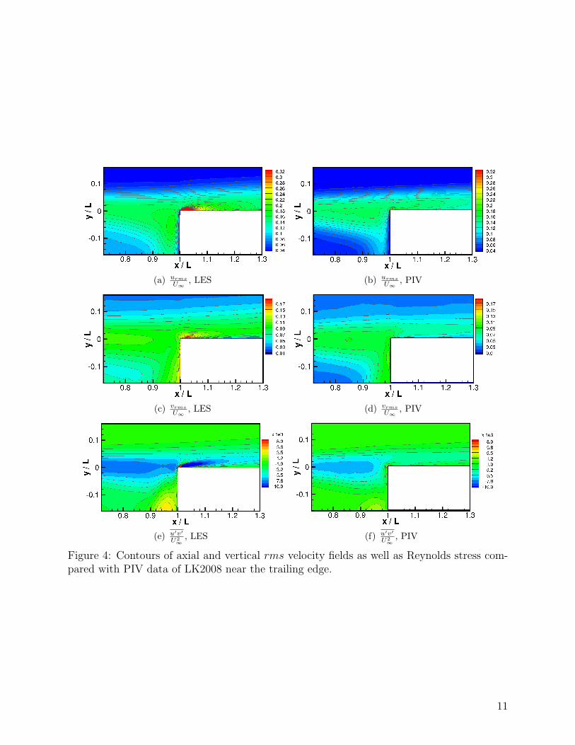
Figure 4 compares the contours of turbulence intensities and Reynolds stress with theexperimental data. Above the trailing edge, there is small recirculation region observed inthe LES studies that is not captured by the PIV data. The mean vertical velocity contours atthe trailing edge are also slightly higher compared to the PIV data. Figure 5 shows verticalvariations in axial rms velocity and Reynolds stress at different axial locations near thetrailing edge for three-different grid resolutions. With grid-refinement, the statistics showimproved predictions in comparison to the experimental data.

The turbulence intensities and Reynolds stresses are reasonably well predicted close tothe trailing edge, but show higher values in a small region slightly above the trailing edge.This may be related to the dynamic subgrid scale viscosity variations in this region involvingcomplex flow patterns. The dynamic subgrid scale model used in this work, requires aver-aging in homogeneous directions for the Smagorinsky constant. In our computation, only alocal averaging was implemented since the flow is developing behind the trailing edge. Withgrid-refinement, this averaging is done on a smaller region and perhaps may contribute tothe over-prediction. It also affects the variation in subgrid viscosity, and this suggests that acareful analysis of subgrid-scale LES models is necessary in this region. In addition, the gridrefinement in the present work is mainly done in the spanwise direction. The wall-normaland the span-wise grids are fine near the wall, this gives very high aspect ratio grid cellsclose to the wall. This may also influence the behavior of the turbulence quantities near thewall. A better distribution of the grid elements in the entire domain reducing the aspectratio of grid cells near the wall may improve the predictions.

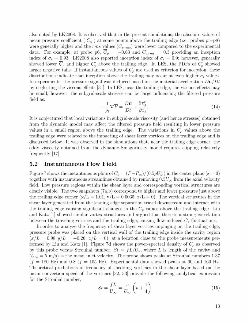
The probability distribution functions (PDFs) of the fluctuations in pressure coefficient(C ′p) at the eight probes (p1–p8) are shown in figure 6 together with location of probes in

the center plane as shown on the Cp contours. The corresponding mean and rms values ofCp are also quoted. Probes p1 and p2 are slightly upstream of the trailing edge, probes p3and p4 are in the shear layer, and probes p5–p8 are downstream of the trailing edge. Basedon the mean values of Cp and the PDFs of C ′p, cavitation is likely to occur inside the shear

layer for a cavitation index of σi ≤∼ 0.43 (for example, for probe p3, Cp = −0.13 with aPDF tail of around −0.3). LK2008 also observed cavitation inside the shear layer for similarinception index. The mean statistics were collected over twelve flow through times, whereone flow through time is taken to be approximately L/U∞.

The probes (p5–p8) above the trailing edge (downstream of the corner) show low valuesof Cp together with a broader spectrum of C ′p. Inception first occurs inside these regions as

10

(a) urms

U∞, LES (b) urms

U∞, PIV

(c) vrms

U∞, LES (d) vrms

U∞, PIV

(e) u′v′

U2∞

, LES (f) u′v′

U2∞

, PIV

Figure 4: Contours of axial and vertical rms velocity fields as well as Reynolds stress com-pared with PIV data of LK2008 near the trailing edge.

11

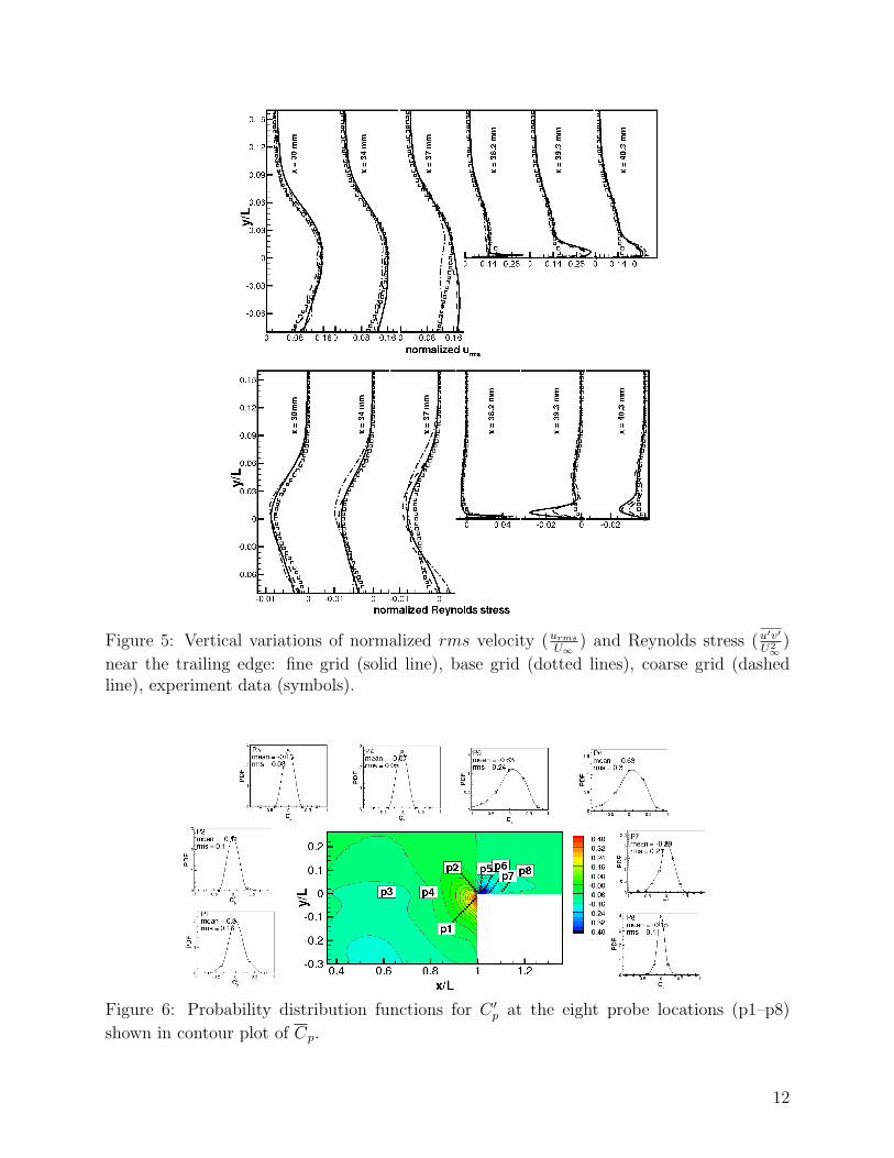
Figure 5: Vertical variations of normalized rms velocity (urms

U∞) and Reynolds stress (u

′v′

U2∞

)

near the trailing edge: fine grid (solid line), base grid (dotted lines), coarse grid (dashedline), experiment data (symbols).

Figure 6: Probability distribution functions for C ′p at the eight probe locations (p1–p8)

shown in contour plot of Cp.

12

also noted by LK2008. It is observed that in the present simulations, the absolute values ofmean pressure coefficient (|Cp|) at some points above the trailing edge (i.e. probes p5–p8)were generally higher and the rms values (Cp,rms) were lower compared to the experimentaldata. For example, at probe p6, Cp = −0.63 and Cp,rms = 0.3 providing an inceptionindex of σi = 0.93. LK2008 also reported inception index of σi = 0.9; however, generallyshowed lower Cp and higher C ′p above the trailing edge. In LES, the PDFs of C ′p showedlarger negative tails. If instantaneous values of Cp are used as criterion for inception, thesedistributions indicate that inception above the trailing may occur at even higher σi values.In experiments, the pressure signal was deduced based on the material acceleration Du/Dtby neglecting the viscous effects [31]. In LES, near the trailing edge, the viscous effects maybe small; however, the subgrid-scale stresses can be large influencing the filtered pressurefield as:

− 1

ρ`∇P =

Du

Dt+∂τ rij∂xj

. (14)

It is conjectured that local variations in subgrid-scale viscosity (and hence stresses) obtainedfrom the dynamic model may affect the filtered pressure field resulting in lower pressurevalues in a small region above the trailing edge. The variations in Cp values above thetrailing edge were related to the impacting of shear layer vortices on the trailing edge and isdiscussed below. It was observed in the simulations that, near the trailing edge corner, theeddy viscosity obtained from the dynamic Smagorinsky model requires clipping relativelyfrequently [17].

5.2 Instantaneous Flow Field

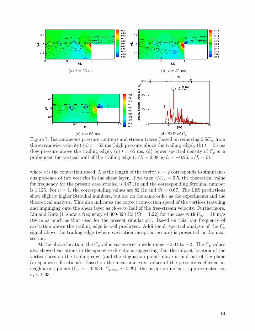
Figure 7 shows the instantaneous plots of Cp = (P−P∞)/(0.5ρU2∞) in the center plane (z = 0)

together with instantaneous streamlines obtained by removing 0.5U∞ from the axial velocityfield. Low pressure regions within the shear layer and corresponding vortical structures areclearly visible. The two snapshots (7a,b) correspond to higher and lower pressures just abovethe trailing edge corner (x/L = 1.01, y/L = 0.0035, z/L = 0). The vortical structures in theshear layer generated from the leading edge separation travel downstream and interact withthe trailing edge causing significant changes in the Cp values above the trailing edge. Liuand Katz [1] showed similar vortex structures and argued that there is a strong correlationbetween the traveling vortices and the trailing edge, causing flow-induced Cp fluctuations.

In order to analyze the frequency of shear-layer vortices impinging on the trailing edge,pressure probe was placed on the vertical wall of the trailing edge inside the cavity region(x/L = 0.98, y/L = −0.26, z/L = 0), at a location close to the probe measurements per-formed by Liu and Katz [1]. Figure 7d shows the power-spectral density of Cp as observedby this probe versus Strouhal number, St = fL/U∞ where L is length of the cavity and(U∞ = 5 m/s) is the mean inlet velocity. The probe shows peaks at Strouhal numbers 1.37(f = 180 Hz) and 0.8 (f = 105 Hz). Experimental data showed peaks at 90 and 160 Hz.Theoretical predictions of frequency of shedding vorticies in the shear layer based on themean convection speed of the vorticies [32, 33] provide the following analytical expressionfor the Strouhal number,

St =fL

U∞=

c

U∞

(n+

1

4

)(15)

13

(a) t = 53 ms (b) t = 55 ms

(c) t = 65 ms (d) PSD of Cp

Figure 7: Instantaneous pressure contours and stream traces (based on removing 0.5U∞ fromthe streamwise velocity):(a) t = 53 ms (high pressure above the trailing edge), (b) t = 55 ms(low pressure above the trailing edge), (c) t = 65 ms, (d) power spectral density of Cp at aprobe near the vertical wall of the trailing edge (x/L = 0.98, y/L = −0.26, z/L = 0).

where c is the convection speed, L is the length of the cavity, n = 2 corresponds to simultane-ous presence of two vorticies in the shear layer. If we take c/U∞ = 0.5, the theoretical valuefor frequency for the present case studied is 147 Hz and the corresponding Strouhal numberis 1.125. For n = 1, the corresponding values are 82 Hz and St = 0.67. The LES predictionsshow slightly higher Strouhal numbers, but are on the same order as the experiments and thetheoretical analysis. This also indicates the correct convection speed of the vortices travelingand impinging onto the shear layer as close to half of the free-stream velocity. Furthermore,Liu and Katz [1] show a frequency of 300-320 Hz (St = 1.22) for the case with U∞ = 10 m/s(twice as much as that used for the present simulation). Based on this, our frequency ofcavitation above the trailing edge is well predicted. Additional, spectral analysis of the Cpsignal above the trailing edge (where cavitation inception occurs) is presented in the nextsection.

At the above location, the Cp value varies over a wide range −0.01 to −2. The Cp valuesalso showed variations in the spanwise directions suggesting that the impact location of thevortex cores on the trailing edge (and the stagnation point) move in and out of the plane(in spanwise directions). Based on the mean and rms values of the pressure coefficient atneighboring points (Cp ∼ −0.639, Cp,rms ∼ 0.29), the inception index is approximated as,σi ∼ 0.93.

14

5.3 Small Scale Cavitation and Inception

We consider two different approaches to investigate the nature of small-scale cavitation nearthe trailing edge and inside the shear layers: (i) a scalar transport model and (ii) a discretebubble model. The results obtained from these two models are described below.Scalar Transport Model: For the scalar-transport model, a transport equation for liquid vol-ume fraction (equation 12) is solved as described earlier. The source and sink terms in thetransport equation are proportional to the difference between the local pressure and thevapor pressure as well as the amount of liquid present in a given control volume. Typi-cally, if the local pressure drops below the vapor pressure, the liquid evaporates creatingvapor. In the present work, the local pressure field was defined relative to the pressure fieldabove the leading edge of the cavity (P∞). Similarly to the experiments, the absolute valueof P∞ was reduced starting with one atmosphere. The vapor pressure was assumed to bePv = 2.337 kPa. Initially, a uniform vapor of φ = 1−Θ` = 10−5 is assumed distributed overthe computational domain. This is based on the dissolved gas concentration estimated inLK2008 for the present case.

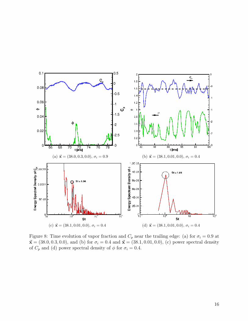
Early sites of cavitation were observed above the trailing edge where the pressure minimaoccur. Small amounts of vapor were created in this region with vapor fractions on the orderof 0.01 for a cavitation index of σi = 0.9.

Figures 8a,b show the temporal variation of vapor fraction (φ = 1−Θ`) and Cp just abovethe trailing edge at two different upstream pressure levels. As can be seen from the timetraces, periodic occurrence and disappearance of cavitation is predicted above the trailingedge. The pressure variations are mainly caused by the shear-layer eddies impinging on thethe cavity trailing edge (see figures 7).

For pressures corresponding to the cavitation index of σi = 0.9, the inception of small-scale cavitation was observed. Further reduction in P∞ resulted in increased amount ofcavitation above the trailing edge. In the experiments, vigorous cavitation was observedfor σi = 0.4. Figures 8c,d show the power-spectral density of the pressure coefficient (Cp)and the scalar (φ) above the trailing edge for σi = 0.4. Strong peaks are observed at thefrequency of 139 Hz and 143 Hz for Cp and φ, respectively. Liu and Katz [1] observed periodiccavitation at frequencies 300-350 Hz for the case of twice the free-stream velocity (10 m/s).For half the free-stream velocity considered here, the convective speed of traveling vorticiesis halved. Power spectra of Cp presented earlier show similar range of periodic frequency forthe vortices impinging on the trailing edge.

In the present work, we do not have pressure-velocity-density coupling, which may becomeimportant when heavy cavitation occurs (for the case of σi ≤ 0.4). However, the featuresassociated with periodic growth and decay of the vapor fraction above the trailing edgeare captured. For this scalar transport model, the local vapor fraction did not exceed unity;however, larger values of φ were observed especially with lower upstream pressures. Pressure-velocity-density coupling may become important under these vigorous cavitation stages andwill be part of a subsequent study.

We decreased the upstream pressure in the scalar transport studies to give σi = 0.1.For this case, cavitation also occurred in the shear layer above the cavity with periodicappearance and disappearance above the trailing edge. The amount of vapor on the shearlayer is mainly generated due to pressure being lower than vapor pressure or Cp < σi = 0.1.

15

(a) ~x = (38.0, 0.3, 0.0), σi = 0.9 (b) ~x = (38.1, 0.01, 0.0), σi = 0.4

(c) ~x = (38.1, 0.01, 0.0), σi = 0.4 (d) ~x = (38.1, 0.01, 0.0), σi = 0.4

Figure 8: Time evolution of vapor fraction and Cp near the trailing edge: (a) for σi = 0.9 at~x = (38.0, 0.3, 0.0), and (b) for σi = 0.4 and ~x = (38.1, 0.01, 0.0), (c) power spectral densityof Cp and (d) power spectral density of φ for σi = 0.4.

16

Liu & Katz [1] also observed vapor bubbles and cavitation in the shear layer for σi < 0.4.Discrete Bubble Model:

We also performed cavitation inception studies using the discrete bubble model (DBM).The gas content in the liquid was assumed to be small (initial gas void fraction was assumedto be 10−5 based on LK2008). It is important for the bubble nuclei to pass through the lowpressure regions above the cavity (‘window of opportunity’ to get drawn into low pressureregions and cavitate) [6]. Accordingly, air nuclei were distributed evenly in a small bandaround the shear layer. The bubbles were initially injected over a small region in the stream-wise direction and in a band of 10 mm in the mid section of flow span. In order to keepthe number of bubbles constant in the domain, bubbles were continuously injected nearthe leading edge and removed further downstream from the trailing edge. To analyze thesensitivity of the initial bubble size to cavitation inception, detailed PDF analysis (followingthe works of Cerutti et al. [8] and Kim et al. [9]) was performed.

Table 2: Case studies to analyze cavitation inception using the Discrete Bubble Model.

Case Figure dinitial σiSymbol (µm)

C1 square 10 0.4C2 triangle 50 0.4C3 circle 100 0.4C4 diamond 50 0.9C5 circle (filled) 50 1.4C6 square (filled) 50 0.1

The initial pressure inside the bubble was set based on an equilibrium radius corre-sponding to the radius of the nuclei and its location in the domain. Using the Rayleigh-Plesset equation at equilibrium conditions, the pressure inside the bubble can be obtainedas: Pb = P out + 2σ/Rb (σ is the surface tension coefficient). The bubbles are then advectedwith ‘one-way’ coupling (bubbles do not affect the flow). On an average, approximately50, 000 bubble trajectories are tracked at each instant. In order to gain better understand-ing of how different parameters such as the initial bubble size and cavitation index σi affectthe inception and the behavior of bubbles, three different initial bubble sizes (10, 50, and100 µm) were considered with a constant cavitation index (σi = 0.4). In addition, fourdifferent cavitation indices (0.1, 0.4, 0.9, and 1.4) were examined on a certain initial bubblediameter (dinit = 50 µm). Table 2 shows different diameters and cavitation indices used inthe present study. Figure 9 shows the temporal evolution of bubble locations inside the shearlayer and above the trailing edge. The size of the scatter symbols is scaled with respect tothe size of the bubble. Accordingly, large size bubbles are obtained near the trailing edge.For σi = 0.4 large size bubbles are readily observed near the trailing edge. As shown later,for this inception index, bubbles inside the shear layer showed the most growth, and rapidvariation in bubble size occurs near the trailing edge. For higher pressure at the upstream(σi = 0.9), bubbles cavitate near the trailing edge; however, little change in size of thebubbles was observed inside the shear layers.

17

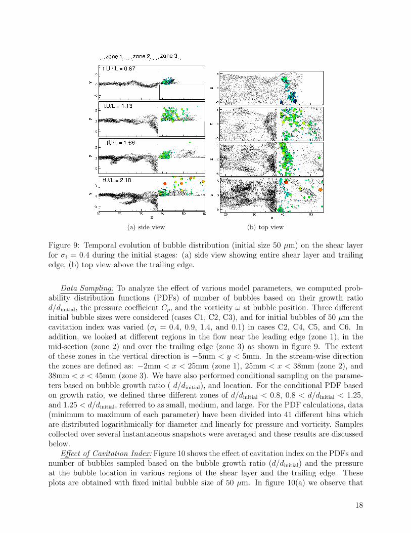
(a) side view (b) top view

Figure 9: Temporal evolution of bubble distribution (initial size 50 µm) on the shear layerfor σi = 0.4 during the initial stages: (a) side view showing entire shear layer and trailingedge, (b) top view above the trailing edge.

Data Sampling: To analyze the effect of various model parameters, we computed prob-ability distribution functions (PDFs) of number of bubbles based on their growth ratiod/dinitial, the pressure coefficient Cp, and the vorticity ω at bubble position. Three differentinitial bubble sizes were considered (cases C1, C2, C3), and for initial bubbles of 50 µm thecavitation index was varied (σi = 0.4, 0.9, 1.4, and 0.1) in cases C2, C4, C5, and C6. Inaddition, we looked at different regions in the flow near the leading edge (zone 1), in themid-section (zone 2) and over the trailing edge (zone 3) as shown in figure 9. The extentof these zones in the vertical direction is −5mm < y < 5mm. In the stream-wise directionthe zones are defined as: −2mm < x < 25mm (zone 1), 25mm < x < 38mm (zone 2), and38mm < x < 45mm (zone 3). We have also performed conditional sampling on the parame-ters based on bubble growth ratio ( d/dinitial), and location. For the conditional PDF basedon growth ratio, we defined three different zones of d/dinitial < 0.8, 0.8 < d/dinitial < 1.25,and 1.25 < d/dinitial, referred to as small, medium, and large. For the PDF calculations, data(minimum to maximum of each parameter) have been divided into 41 different bins whichare distributed logarithmically for diameter and linearly for pressure and vorticity. Samplescollected over several instantaneous snapshots were averaged and these results are discussedbelow.

Effect of Cavitation Index: Figure 10 shows the effect of cavitation index on the PDFs andnumber of bubbles sampled based on the bubble growth ratio (d/dinitial) and the pressureat the bubble location in various regions of the shear layer and the trailing edge. Theseplots are obtained with fixed initial bubble size of 50 µm. In figure 10(a) we observe that

18

(a) (b)

(c) (d)

(e) (f)

(g) (h)

Figure 10: Effect of cavitation index σi on the PDFs and average number of bubbles (Nb)sampled based on the growth ratio (d/dinitial) and pressure coefficient Cp for case C2 (σi = 0.4,triangle symbols), C4 (σi = 0.9, diamond symbols), C5 (σi = 1.4, filled circles), and C6(σi = 0.1, filled square): (a,b) PDF of all bubbles over the region of interest; (c,d) bubblesin zone 1; (e,f) bubbles in zone 2, and (g,h) bubbles in zone 3.

19

a majority of the bubbles retain their original size and are mostly insensitive to pressurevariations (d/dinitial ∼ 1). With lower cavitation index (σi = 0.1), the maximum bubblegrowth ratio is higher, and a small number of very large bubbles are observed near thetrailing edge (giving rise to cavities on the order of 0.1-0.5 cm). This is due to the effectof lower pressure on the bubbles compared to the cases with σi = 0.9 and 1.4. The otherimportant difference is on the left tail of PDF (collapse region) where the PDF of growthratio is almost an order of magnitude larger for σi = 0.9 compared to σi = 0.4. This againindicates violent cavitation for lower cavitation index. Next we consider the behavior ofbubbles in the different zones as described earlier. Figures 10c-h show average number ofbubbles sampled based on the growth ratio and Cp values. In zones 1 and 2 (i.e. insidethe shear layer), their is small change in the average number of bubbles versus a certaingrowth ratio for different cavitation indices; however, for σi = 0.1 and 0.4 more variation inbubble sizes were observed in both zones (figures 10(c),10(e)). Near the trailing edge, largedifferences in the number of bubbles with the same growth ratio are observed (figure 10(g)).For the lowest σi (C6), number of large bubbles observed near the trailing edge is at least anorder of magnitude more than other cases (C2, C4, and C5). The highest cavitation indexnearly shows no cavitation above trailing edge.

Figure 10(b) shows the PDF of Cp at bubble locations for cases C2, C4, C5, and C6 overthe entire region of interest. Changing σi doesn’t change the PDF curves sampled based onCp appreciably; implying that the location of bubbles is not significantly affected by varyingσi. This can also be observed in the snapshots of bubbles in figure 9. Figures 10(d), 10(f),and 10(h) show the average number of bubbles sampled based on Cp in zones 1 (near leadingedge), 2 (midsection), and 3 (near trailing edge), respectively. Noticeable number of bubblesare observed in the range of −1 ≤ Cp ≤ 1. This is consistent with the experiments, whereinLiu and Katz [1] predicted cavitation inception occurs at σi = 0.9. These plots also indicatepresence of large number of bubbles in the low pressure region for σi = 0.1 and 0.4. Basedon the growth ratios, these are typically larger size bubbles which get attracted toward thelow pressure region.

(a) (b)

Figure 11: Average number of conditionally sampled bubbles based on pressure coefficient atbubble location for case C1 (square), C2 (triangle), and C3 (circle): (a) medium size group(0.8 < d/dinitial < 1.25), (b) large size group (1.25 < d/dinitial).

Effect of Initial Bubble Size: The effect of initial bubble size (figure not shown) is alsoinvestigated by computing PDFs of growth ratio and Cp for cases C1, C2, and C3 over theentire region and in different zones [17]. It was observed that the growth of the smaller

20

bubbles (10 microns) is less responsive to pressure changes. A majority of them grow toabout 3-4 times their original size, whereas a very few become 100 times larger. This may beattributed to the fact that smaller bubbles tend to travel with the flow (low Stokes number),thus, fewer are expected to be entrained into the lower pressure region. Larger bubbles (50and 100 microns) can grow to very large size (10-100 times the initial size). Based on thegrowth ratio, 50 and 100 micron bubbles seem to be entrained in the low pressure regionsin the shear layer (zones 1 and 2) and show some growth (less than twice the initial size) inthese regions for σi = 0.4. Near the trailing edge, however, rapid growth in size is observedfor these bubbles; some growing up to 50 times their original size. Correspondingly, theycreate cavities on the order of 0.5 cm also observed in the experiments.

Conditional Sampling and Bubble Distributions: To further characterize the sensitivityof the bubbles to imposed pressure variations, the bubbles were sampled into three groupsbased on their growth ratio: small (d/dinitial < 0.8), medium (0.8 < d/dinitial < 1.25), andlarge (1.25 < d/dinitial) bubbles. Bubbles from each group were then conditionally sampledto obtain PDFs and average number of bubbles based on Cp (figure 11) and vorticity ωdistributions (not shown). Figures 11a,b show that bubbles with an initial size of 10 micronstend to remain in the medium group (i.e. 0.8 < d/dinitial < 1.25), whereas larger initial sizebubbles (50 and 100 micron) exhibit large growth (1.25 < d/dinitial). This indicates thatbubbles with an initial size in the range of 50-100 microns are capable of predicting visiblecavitation. Similar conclusions were drawn for plots based on vorticity distribution [17]. Thisindicates that small initial size bubbles, although sensitive to pressure fluctuations, do nottend to cluster in regions of high vorticity or low pressure. To predict cavitation inception,initial bubble sizes on the order of 50-100 micron are best suited for the present case as theytend to cluster in low pressure regions and thus can grow to large sizes. However, for otherconfigurations, such as flow over hydrofoils, small bubbles can entrain quickly into the lowpressure regions and be sensitive to rapid pressure variations.

6 Comparison of Scalar Transport and Discrete Bub-

ble Models

In order to make a quantitative comparison of the two models in capturing small scalecavitation, we compute the temporal evolution of the expansion ratio predicted by the twomodels above the tailing edge in zone 3. The expansion ratio is a volume-averaged quantityrepresenting the average growth in vapor fraction in a specified region compared to the initialvapor fraction and is defined as,

Expansion Ratio =

∑V φ

tcvVcv∑

V φ0cvVcv

(scalar transport model), (16)

=

∑b V

tb∑

b V0b

(discrete bubble model). (17)

Here, Vcv is the cv volume, Vb is the bubble volume, the superscripts ‘t’ and ‘0’ correspondto current and initial time level, and the summation (volume averaging) is carried out over

21

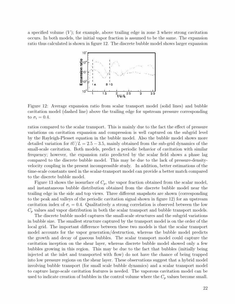
a specified volume (V ); for example, above trailing edge in zone 3 where strong cavitationoccurs. In both models, the initial vapor fraction is assumed to be the same. The expansionratio thus calculated is shown in figure 12. The discrete bubble model shows larger expansion

Figure 12: Average expansion ratio from scalar transport model (solid lines) and bubblecavitation model (dashed line) above the trailing edge for upstream pressure correspondingto σi = 0.4.

ratios compared to the scalar transport. This is mainly due to the fact the effect of pressurevariations on cavitation expansion and compression is well captured on the subgrid levelby the Rayleigh-Plesset equation in the bubble model. Also the bubble model shows moredetailed variation for tU/L = 2.5− 3.5, mainly obtained from the sub-grid dynamics of thesmall-scale cavitation. Both models, predict a periodic behavior of cavitation with similarfrequency; however, the expansion ratio predicted by the scalar field shows a phase lagcompared to the discrete bubble model. This may be due to the lack of pressure-density-velocity coupling in the present incompressible study. In addition, better estimations of thetime-scale constants used in the scalar-transport model can provide a better match comparedto the discrete bubble model.

Figure 13 shows the isosurface of Cp, the vapor fraction obtained from the scalar model,and instantaneous bubble distribution obtained from the discrete bubble model near thetrailing edge in the side and top views. Three different snapshots are shown (correspondingto the peak and valleys of the periodic cavitation signal shown in figure 12) for an upstreamcavitation index of σi = 0.4. Qualitatively a strong correlation is observed between the lowCp values and vapor distribution in both the scalar transport and bubble transport models.

The discrete bubble model captures the small-scale structures and the subgrid variationsin bubble size. The smallest structure captured by the transport model is on the order of thelocal grid. The important difference between these two models is that the scalar transportmodel accounts for the vapor generation/destruction, whereas the bubble model predictsthe growth and decay of gaseous bubbles. The scalar transport model could capture thecavitation inception on the shear layer, whereas discrete bubble model showed only a fewbubbles growing in this region. This may be due to the fact that bubbles (initially beinginjected at the inlet and transported with flow) do not have the chance of being trappedinto low pressure regions on the shear layer. These observations suggest that a hybrid modelinvolving bubble transport (for small scale bubble dynamics) and a scalar transport modelto capture large-scale cavitation features is needed. The vaporous cavitation model can beused to indicate creation of bubbles in the control volume where the Cp values become small.

22

Figure 13: Instantaneous isosurfaces of Cp = −0.25 (left panel), and φ = 0.25 (middle panel),and bubble scatter plot (right panel) for three time levels corresponding to the expansionratio signal in figure 12: time level A (top panels), time level B (middle panel), and timelevel C (bottom panels). Scatter symbols are scaled to bubble size relative to the grid.

23

As the bubbles grow, an approach coupling the Lagrangian discrete bubbles with an Eulerianscalar field is needed to better represent the broad range of scales observed in cavitation.

7 CONCLUSIONS

We performed LES of turbulent flow over an open cavity corresponding to the experimentalsetup of Liu and Katz [1] at the flow Reynolds number of 170, 000. The filtered, incompress-ible Navier-Stokes equations were solved using a co-located grid finite-volume solver usingthe dynamic Smagorinsky model. Three different grid resolutions, with mainly Cartesianhexahedral elements, were considered to obtain grid independent flow statistics. The meanflowfield at the inlet section is specified from the experimental data in the symmetry plane,whereas, turbulent fluctuations were imposed at the inflow based on resolved computationof a periodic duct flow keeping the mass-flow rate and the Reynolds number the same. Theflow statistics, including mean and rms velocity fields, showed reasonable agreement with theexperimental data near the leading and the trailing edges. The mean pressure distributionshows two distinct features near the trailing edge: (i) a high-pressure region just upstream ofthe trailing edge which extends slightly into the cavity, and (ii) a low pressure region abovethe trailing edge. The high pressure region just upstream of the trailing edge occurs mainlydue to the impingement of the shear layer onto to the trailing edge, creating a stagnationpoint inside the cavity. The sharp corner, downstream of the stagnation point, causes lowpressure region above the trailing edge. Variations in local Cp values above the trailingedge were also investigated and showed correlations with the impingement of the shear layervortices onto the trailing edge.

Small-scale cavitation and inception were investigated using two approaches: (i) a discretebubble model for gaseous cavitation wherein the bubble dynamics is computed by solving theRayleigh-Plesset and bubble motion equations using an adaptive time-stepping procedure,and (ii) a scalar transport based model for the liquid volume fraction with source and sinkterms for phase change corresponding to vaporous cavitation. In both models, the effectof bubbles or vapor on the flowfield was neglected. Simulations with different values ofthe upstream pressure were performed by changing the cavitation index (σi). Both modelspredicted that inception occurs above the trailing edge. For σi < 0.4, heavy cavitation wasobserved above the trailing edge. The scalar transport model predicted periodic growth anddecay of the liquid vapor fraction above the trailing edge owing to local variations in pressureminima. The frequency of vortex shedding as obtained based on the pressure signal is closeto the theoretical prediction and also is in agreement with the experimental observations.The scalar transport model was also able to predict the cavitation inception on the shearlayer for a cavitation index of 0.1. Inception on the shear layer was found to be mainly dueto generation of vapor as the local pressure falls below vapor pressure.

The discrete bubble model captures the subgrid dynamics of bubbles and also showscavitation inception occurring above the trailing edge. For low σi, rapid variations in bubblesizes were also observed within the shear layer. The discrete bubble model, however, couldnot predict large amounts of cavitation within the shear layer. Sensitivity to initial bubblesize and the cavitation index were investigated in detail; it was found that 50-100 micronbubbles tend to cluster in low pressure regions and exhibit more growth. By examining the

24

probablity distribution functions and average number of bubbles, the inception index of 0.9agrees well with the experimental data.

In order to make a quantitative comparison between the two models in capturing smallscale cavitation, the temporal evolution of the vapor expansion ratio, defined as a volume-averaged quantity representing the average growth in vapor fraction in a specified regioncompared to the initial vapor fraction, was computed above the tailing edge. Both mod-els indicate a periodic variation in the expansion ratio with periods corresponding to thecavitation process observed in experiment.

The present LES study indicates that the classical inception model, Cp < −σi, is notsufficient for description of inception dynamics in this flow. It was found that, Cp = −0.63on top of the trailing edge, whereas small-scale cavitation was observed for σi = 0.9 near thetrailing edge in both models. The flow over an open cavity, represents a complex flow withflow separation, shear layer and interaction of the shear layer with the trailing edge. We haveshown that the LES methodology together with cavitation models based on scalar and dis-crete bubble transport can predict the unsteady behavior of small-scale cavitation. To avoidthe overprediction of eddy viscosity near the trailing edge, further analysis/development ofsubgrid scale viscosity models for LES in regions where the shear-layer vorticies impingeupon the trailing edge is needed. Subgrid scale models for anisotropic grids together withuniform distribution of grids near the trailing edge (making use of unstructured grids, forexample) may help improve the LES predictions.

In this geometry, strong fluctuations in flow are observed on top of the trailing edge andon the shear layer. These fluctuations govern the vapor generation and bubble size variationsin the cavitation models, through rapid variations in pressure and flow acceleration. Thecavitation models used in the present study do not involve velocity-density-pressure coupling.In regions of vigorous cavitation (above the trailing edge), this assumption may not beaccurate in the large cavity regions, and such coupling should be considered in future studies.The present study indicates that, a combination of the scalar-transport as well as discrete-bubble model for small scale cavitation is necessary capturing effects of phase transfer aswell as pressure oscillations on subgrid bubble nuclei.

8 Acknowledgment

This work was supported by the Office of Naval Research (ONR) grant number N000140610697.The program manager is Dr. Ki-Han Kim. We thank Prof. Joseph Katz and Dr. XiaofengLiu of Johns Hopkins University for the experimental data as well as useful discussions.

References

[1] Liu, X. and Katz, J., 2008, “Cavitation phenomena occurring due to interaction ofshear layer vortices with the trailing corner of a two-dimensional open cavity.” Physicsof Fluids, 20(4).

[2] Arndt, R., 2002, “Cavitation in vortical flows.” Annual Review of Fluid Mechanics,34(1), pp. 143–175.

25

[3] Rood, E., 1991, “Review: Mechanisms of cavitation inception,” Journal of Fluids En-gineering, 113(2), pp. 163–175.

[4] Johnson, V. and Hsieh, T., 1966, “The influence of the trajectories of gas nuclei oncavitation inception,” Sixth Symposium on Naval Hydrodynamics, pp. 163–179.

[5] Hsiao, C. and Chahine, G., 2008, “Numerical study of cavitation inception due tovortex/vortex interaction in a ducted propulsor,” Journal of Ship Research, 52(2), pp.114–123.

[6] Hsiao, C., Jain, A., and Chahine, G., 2006, “Effect of Gas Diffusion on Bubble En-trainment and Dynamics around a Propeller,” Proceedings of 24th Symposium on NavalHydrodynamics, Rome Italy, vol. 26.

[7] De Chizelle, Y. K., Ceccio, S. L., and Brennen, C. E., 1995, “Observations and scalingof travelling bubble cavitation,” Journal of Fluid Mechanics Digital Archive, 293(-1),pp. 99–126.

[8] Cerutti, S., Knio, O., and Katz, J., 2000, “Numerical study of cavitation inception inthe near field of an axisymmetric jet at high Reynolds number,” Physics of Fluids, 12,p. 2444.

[9] Kim, J., Paterson, E., and Stern, F., 2006, “RANS simulation of ducted marine propul-sor flow including subvisual cavitation and acoustic modeling,” Journal of Fluids Engi-neering, 128, p. 799.

[10] Farrell, K., 2003, “Eulerian/Lagrangian analysis for the prediction of cavitation incep-tion,” Journal of Fluids Engineering, 125(1), pp. 46–52.

[11] Alehossein, H. and Qin, Z., 2007, “Numerical analysis of Rayleigh–Plesset equation forcavitating water jets,” Int. J. Numer. Meth. Engng, 72, pp. 780–807.

[12] Wienken, W., Stiller, J., and Keller, A., 2006, “A method to predict cavitation inceptionusing large-eddy simulation and its application to the flow past a square cylinder,”Journal of Fluids Engineering, 128, p. 316.

[13] Germano, M., Piomelli, U., Moin, P., and Cabot, W., 1991, “A dynamic subgrid-scaleeddy viscosity model,” Physics of Fluids A: Fluid Dynamics, 3, p. 1760.

[14] Merkle, C. L., Feng, J., and Buelow, P., 1998, “Computational modeling of the dynamicsof sheet cavitation,” Proceedings of the 3rd International Symposium on Cavitation(CAV ’98), Grenoble, France.

[15] Senocak, I. and Shyy, W., 2004, “Interfacial dynamics-based modelling of turbulent cav-itating ows, Part-1: Model development and steady-state computations,” InternationalJournal for Numerical Methods in Fluids, 44, pp. 975–995.

[16] Hsiao, C. and Chahine, G., 2002, “Prediction of vortex cavitation inception using cou-pled spherical and non-spherical models and UnRANS computations,” Proceedings of24th Symposium on Naval Hydrodynamics, Fukuoka, Japan.

26

[17] Sobhani, S. et al., 2010, Numerical simulation of cavitating bubble-laden turbulent flows,Ph.D. thesis, Oregon State University.

[18] Brennen, C., 1995, Cavitation and bubble dynamics, Oxford University Press, USA.

[19] Chahine, G., 1994, “Strong interactions bubble/bubble and bubble/flow,” IUTAM con-ference on bubble dynamics and interfacial phenomena (ed. JR Blake). Kluwer.

[20] Apte, S., Mahesh, K., and Lundgren, T., 2008, “Accounting for finite-size effects insimulations of disperse particle-laden flows,” International Journal of Multiphase Flow,pp. 260–271.

[21] Darmana, D., Deen, N., and Kuipers, J., 2006, “Parallelization of an Euler–Lagrangemodel using mixed domain decomposition and a mirror domain technique: Applicationto dispersed gas–liquid two-phase flow,” Journal of Computational Physics, 220(1), pp.216–248.

[22] Apte, S., Shams, E., and Finn, J., 2009, “A hybrid Lagrangian-Eulerian approach forsimulation of bubble dynamics,” Proceedings of the 7th International Symposium onCavitation, CAV2009, Ann Arbor, Michigan, USA. (submitted).

[23] Singhal, A., Vaidya, N., and Leonard, A., 1997, “Multi-dimensional simulation of cavi-tating flows using a PDF model for phase change,” ASME Paper FEDSM97-3272, the1997 ASME Fluids Engineering Division Summer Meeting.

[24] Senocak, I. and Shyy, W., 2004, “Interfacial dynamics-based modelling of turbulent cav-itating ows, part-2: time-dependent computations,” International Journal for NumericalMethods in Fluids, 44, pp. 997–1016.

[25] Senocak, I. and Shyy, W., 2002, “Evaluation of Cavitation Models for Navier-StokesComputations,” FEDSM2002-31011, Proc. of 2002 ASME Fluids Engineering DivisionSummer Meeting Montreal, CA.

[26] Mahesh, K., Constantinescu, G., and Moin, P., 2004, “A numerical method for large-eddy simulation in complex geometries,” J. Comput. Phys., 197(1), pp. 215–240.

[27] Mahesh, K., Constantinescu, G., Apte, S., Iaccarino, G., Ham, F., and Moin, P., 2006,“Large-eddy simulation of reacting turbulent flows in complex geometries,” J. AppliedMech., 73, p. 374.

[28] Moin, P. and Apte, S., 2006, “Large-eddy simulation of realistic gas turbine-combustors,” AIAA Journal, 44(4), pp. 698–708.

[29] Apte, S., Mahesh, K., Moin, P., and Oefelein, J., 2003, “Large-eddy simulation ofswirling particle-laden flows in a coaxial-jet combustor,” International Journal of Mul-tiphase Flow, 29(8), pp. 1311–1331.

[30] Pierce, C. and Moin, P., 1998, “Large eddy simulation of a confined coaxial jet withswirl and heat release,” AIAA Paper, 2892.

27

[31] Liu, X. and Katz, J., 2006, “Instantaneous pressure and material acceleration measure-ments using a four-exposure PIV system,” Experiments in Fluids, 41(2), pp. 227–240,URL http://dx.doi.org/10.1007/s00348-006-0152-7.

[32] Martin, W., Naudascher, E., and Padmanabhan, M., 1975, “Fluid-dynamic excitationinvolving flow instability,” Journal of Hydraulic Division, 101, p. 681.

[33] Blake, W., 1986, Mechanics of flow-induced sound and vibration, Academic, New York,1986.

28