SANDIA REPORT SAND2007-5948 Unlimited Release Printed October 2007

Predictive Capability Maturity Model for Computational Modeling and Simulation William L. Oberkampf, Martin Pilch, and Timothy G. Trucano Prepared by Sandia National Laboratories Albuquerque, New Mexico 87185 and Livermore, California 94550 Sandia is a multiprogram laboratory operated by Sandia Corporation, a Lockheed Martin Company, for the United States Department of Energy’s National Nuclear Security Administration under Contract DE-AC04-94AL85000. Approved for public release; further dissemination unlimited.

2

Issued by Sandia National Laboratories, operated for the United States Department of Energy by Sandia Corporation. NOTICE: This report was prepared as an account of work sponsored by an agency of the United States Government. Neither the United States Government, nor any agency thereof, nor any of their employees, nor any of their contractors, subcontractors, or their employees, make any warranty, express or implied, or assume any legal liability or responsibility for the accuracy, completeness, or usefulness of any information, apparatus, product, or process disclosed, or represent that its use would not infringe privately owned rights. Reference herein to any specific commercial product, process, or service by trade name, trademark, manufacturer, or otherwise, does not necessarily constitute or imply its endorsement, recommendation, or favoring by the United States Government, any agency thereof, or any of their contractors or subcontractors. The views and opinions expressed herein do not necessarily state or reflect those of the United States Government, any agency thereof, or any of their contractors. Printed in the United States of America. This report has been reproduced directly from the best available copy. Available to DOE and DOE contractors from U.S. Department of Energy Office of Scientific and Technical Information P.O. Box 62 Oak Ridge, TN 37831 Telephone: (865) 576-8401 Facsimile: (865) 576-5728 E-Mail: reports@adonis.osti.gov Online ordering: http://www.osti.gov/bridge Available to the public from U.S. Department of Commerce National Technical Information Service 5285 Port Royal Rd. Springfield, VA 22161 Telephone: (800) 553-6847 Facsimile: (703) 605-6900 E-Mail: orders@ntis.fedworld.gov Online order: http://www.ntis.gov/help/ordermethods.asp?loc=7-4-0#online

3

SAND2007-5948 Unlimited Release

Printed October 2007

Predictive Capability Maturity Model for Computational Modeling and Simulation

William L. Oberkampf and Martin Pilch Validation and Uncertainty Quantification Department

Timothy G. Trucano Optimization and Uncertainty Estimation Department

Sandia National Laboratories

P. O. Box 5800 Albuquerque, New Mexico 87185-0828

Abstract

The Predictive Capability Maturity Model (PCMM) is a new model that can be used to assess the level of maturity of computational modeling and simulation (M&S) efforts. The development of the model is based on both the authors’ experience and their analysis of similar investigations in the past. The perspective taken in this report is one of judging the usefulness of a predictive capability that relies on the numerical solution to partial differential equations to better inform and improve decision making. The review of past investigations, such as the Software Engineering Institute’s Capability Maturity Model Integration and the National Aeronautics and Space Administration and Department of Defense Technology Readiness Levels, indicates that a more restricted, more inter-pretable method is needed to assess the maturity of an M&S effort. The PCMM addresses six contributing elements to M&S: (1) representation and geometric fidelity, (2) physics and material model fidelity, (3) code verification, (4) solution verification, (5) model validation, and (6) uncertainty quantification and sensitivity analysis. For each of these elements, attributes are identified that characterize four increasing levels of maturity. Importantly, the PCMM is a structured method for assessing the maturity of an M&S effort that is directed toward an engineering application of interest. The PCMM does not assess whether the M&S effort, the accuracy of the predictions, or the performance of the engineering system satisfies or does not satisfy specified application requirements.

4

Acknowledgements We thank the following NASA staff for many helpful discussions and comments in the development of the PCMM: Steve Blattnig, Larry Green, Mike Hemsch, Karen Lyle, Jim Luckring, Joe Morrison, Ram Tripathi and Thomas Zang of Langley Research Center; Joe Hale, Kevin Tucker, and Jeffery West of Marshall Space Flight Center; Martin Steele of Kennedy Space Center; Maria Babula of Glenn Research Center; Gary Mosier of Goddard Space Flight Center; Bill Bertch of Jet Propulsion Laboratory; Andre Sylvester of Johnson Space Center; and Harold Bell of NASA’s Office of Chief Engineer. We also thank Simone Youngblood, of Johns Hopkins Applied Physics Laboratory, and Scott Harmon, consultant, for their valuable feedback on the Predictive Capability Maturity Model. David Peercy of Sandia National Laboratories also provided insightful review comments and suggestions for improving the concepts and clarity of our ideas. Finally, we thank Rhonda Reinert of Technically Write for providing extensive editorial assistance during the writing of this report.

5

Contents Executive Summary ....................................................................................................................7 Acronyms ...................................................................................................................................9

1. Introduction........................................................................................................................10 1.1 The Value of M&S ..................................................................................................10 1.2 Outline of the Report ...............................................................................................11

2. Review of the Literature.....................................................................................................13

3. Aspects of Predictive Capability.........................................................................................21 3.1 Physics Modeling Fidelity .......................................................................................21 3.2 Code Verification ....................................................................................................23 3.3 Solution Verification................................................................................................25 3.4 Model Validation and Uncertainty Quantification ....................................................26 3.5 Level of Maturity.....................................................................................................30

4. Proposed Predictive Capability Maturity Model .................................................................33 4.1 Purpose and Uses of the PCMM ..............................................................................33 4.2 Characteristics of PCMM Elements .........................................................................37

4.2.1 Representation and Geometric Fidelity.........................................................39 4.2.2 Physics and Material Model Fidelity ............................................................40 4.2.3 Code Verification.........................................................................................41 4.2.4 Solution Verification....................................................................................42 4.2.5 Model Validation .........................................................................................43 4.2.6 Uncertainty Quantification and Sensitivity Analysis.....................................45

5. Additional Uses of the Predictive Capability Maturity Model ............................................48 5.1 Requirements for Modeling and Simulation Maturity...............................................48 5.2 Aggregation of PCMM Scores .................................................................................50 5.3 Use of the PCMM in Risk-Informed Decision Making.............................................51

6

Figures Figure 1: Example of Two Basic Types of Coupling of Physical Phenomena. ...........................23 Figure 2: Integrated View of Code Verification in M&S [20, 21]. .............................................24 Figure 3: Three Aspects of Model Validation [37].....................................................................26 Figure 4: Example of a Validation Hierarchy for a Hypersonic Cruise Missile [20, 21]. ............29 Figure 5: Factors Influencing Risk-informed Decision Making..................................................51

Tables Table 1: Table Format for PCMM Assessment ..........................................................................34 Table 2: Example of Predictive Capability Maturity Model after Maturity Assessment .............35 Table 3: General Descriptions for Table Entries of the PCMM..................................................38 Table 4: Example of PCMM Table Assessment and Project Maturity Requirements .................49

7

Executive Summary During the last few decades, modeling and simulation (M&S) has dramatically impacted how engineered systems are designed and how the performance, reliability, and safety of these systems are assessed. In this report, we are interested in M&S efforts that rely heavily on large-scale computer codes to solve complex, nonlinear partial differential equations (PDEs) or integro-differential equations. M&S is commonly thought of as a general-purpose capability, but our perspective is of M&S directed toward a specified engineering application. Over the last two decades, the application of M&S to complex systems has conclusively demonstrated a number of elements that are crucial to predictive capability. Examples are the very large-scale risk assessment efforts applied to nuclear power reactors and the underground storage of nuclear waste. With continually increasing resources devoted to the development of an M&S capability and increasing reliance placed on M&S in decision making, it is necessary to develop improved methods for assessing the quality of M&S activities.

We review efforts that have addressed closely related maturity assessment issues, including the Capability Maturity Model Integration (CMMI) developed by the Software Engineering Institute, the Technology Readiness Levels developed by the National Aeronautics and Space Administration (NASA) and the Department of Defense, NASA’s recent effort to develop an M&S interim standard, and various individual research activities. When we attempted to use these approaches, we concluded that their primary shortcoming was representational information quality, specifically, interpretability. That is, previous work lacked a clear and unambiguous meaning of what the information meant and how it should be used.

We propose the Predictive Capability Maturity Model (PCMM), which is a structured method for assessing the level of maturity of M&S efforts. The purpose of the PCMM is to contribute to decision making for some engineering system applications. The six M&S elements used to assess maturity in this model are (1) representation and geometric fidelity, (2) physics and material model fidelity, (3) code verification, (4) solution verification, (5) model validation, and (6) uncertainty quantification and sensitivity analysis. These six elements are important in judging the trustworthiness and credibility of an M&S effort that deals primarily with the numerical solution of PDEs describing the engineering system of interest.

Representation and geometric fidelity is directed toward the level of detailed characterization of the system being analyzed or specification of the geometrical features of that system.

Physics and material model fidelity deals primarily with (1) the degree to which models are physics based, (2) the degree to which the models are calibrated, (3) the degree to which the models are being extrapolated from the validation and calibration database to the conditions of the application of interest, and (4) the quality and degree of coupling of multiphysics effects that exist in the application of interest.

Code verification focuses on (1) correctness and fidelity of the numerical algorithms used in the code relative to the mathematical model (the PDE model); (2) correctness of the source code; and (3) configuration management, control, and testing of software through SQE practices.

8

Solution verification deals with (1) assessment of numerical solution errors in the computed results and (2) assessment of confidence in the computational results as the results may be affected by human errors.

Model validation concentrates on (1) thoroughness and precision of the accuracy assessment of the computational results relative to the experimental measurements; (2) completeness and precision of the characterization of the experimental conditions and measurements; and (3) relevancy of the experimental conditions, physical hardware, and measurements in the validation experiments compared to the application of interest.

Uncertainty quantification and sensitivity analysis focuses on (1) thoroughness and soundness of the uncertainty quantification effort, including the identification and characterization of all plausible sources of uncertainty; (2) accuracy and correctness of propagating uncertainties through a computational model and interpreting uncertainties in the system response quantities of interest; and (3) thoroughness and precision of a sensitivity analysis to determine the most important contributors to uncertainty in system responses.

Each of the six elements is assessed with respect to descriptive characteristics that are divided into four levels (0, 1, 2, and 3), as follows: level 0, little or no assessment of accuracy and completeness and highly reliant on personal judgment and experience; level 1, some informal assessment of accuracy and completeness, and some assessment has been made by an internal peer review group; level 2, some formal assessment of accuracy and completeness, and some assessments have been made by an external peer review group; and level 3, formal assessment of accuracy and completeness, and essentially all assessments have been made by an independent, external peer review group.

This maturity scale assesses the maturity of an M&S effort, or process, directed toward an engineering system of interest. The scale, by itself, does not assess whether the M&S effort, the accuracy of the predictions, or the performance of the engineering system satisfies a set of imposed requirements. We believe the summary information in the PCMM table will prove beneficial in a number of environments, for example:

• Conducting a PCMM assessment and sharing it with interested parties and stakeholders engenders discussions that would not have occurred without the assessment. Such communication is a highly significant consequence of an M&S maturity assessment.

• By using the PCMM over time, progress in the M&S effort can be tracked. This is useful for M&S managers, decision makers using the results of the M&S effort, and M&S funding sources to determine progress or value added over time.

We also discuss aggregating PCMM scores, for example, from multiple subsystems. Although we recommend that PCMM scores not be aggregated, our experience with using the PCMM shows that various pressures, such as high-level M&S maturity reviews, require some type of compression of PCMM scoring. We recommend a summary method that always maintains a minimum value, an average value, and a maximum value through any aggregation process. We conclude the report by explaining how PCMM scores are only part of the information that should be considered by decision makers concerned with engineering systems.

9

Acronyms AIAA American Institute of Aeronautics and Astronautics ASC Advanced Simulation and Computing ASME American Society of Mechanical Engineers BC boundary condition CAD computer-aided design CAM computer-aided manufacturing CMM Capability Maturity Model CMMI Capability Maturity Model Integration CMMI-DEV Capability Maturity Model Integration-Development DoD Department of Defense F&C features and capabilities I/O input/output IC initial condition IEEE Institute of Electrical and Electronics Engineers IET integral effects test M&S modeling and simulation NASA National Aeronautics and Space Administration NNSA National Nuclear Security Administration PCMM Predictive Capability Maturity Model PDE partial differential equation PIRT Phenomena Identification and Ranking Table QMU quantification of margins and uncertainties SA sensitivity analysis SET separate effects test SQE software quality engineering SRQ system response quantity TRL Technology Readiness Level UQ uncertainty quantification V&V verification and validation WIPP Waste Isolation Pilot Plant

10

1. Introduction During the last few decades, modeling and simulation (M&S) has dramatically impacted how engineered systems are designed and how the performance, reliability, and safety of these systems are assessed.The role of M&S is particularly important in designing and assessing the performance of high-consequence systems, such as those that model the operations of nuclear power plants, the long-term underground storage of nuclear waste, and the safety of nuclear weapons. Simulations of high-consequence systems must demonstrate exceptionally high levels of quality in terms of both credibility, and interpretability. For example, the results produced by the simulations must be believable and presented in a way that enhances understanding. Similarly, the M&S efforts of which these simulations are a part must be characterized in a way that concisely captures the activities that were accomplished to generate the simulation results. Here, we are interested in M&S efforts that rely heavily on large-scale computer codes to solve complex, nonlinear partial differential equations (PDEs) or integro-differential equations. Although M&S has made great strides during the last few decades, we believe the quality and maturity of the assessment procedures for all contributing elements to M&S are still in the early stages of development. In contrast, for example, procedures developed to assess the interpretability and maturity of experimental-measurement uncertainty estimation are of a much higher state of development than analogous procedures in M&S.

1.1 The Value of M&S

M&S provides value for engineered systems in various ways. For example, M&S can

• decrease the time it takes to get a new product to market,

• improve optimization of a system’s performance prior to production of that system,

• potentially reduce the cost of the traditional test-break-fix engineering design cycle, and

• provide an ability for assessing the reliability and safety of a system in environments and failure-mode conditions that cannot be tested.

The most common theme underlying the value of M&S in the example given above is its ability for prediction, i.e., the ability to forecast system responses under specific conditions of the system and the environment. The ability for prediction is usually referred to as predictive power in scientific theory. In science, predictive power commonly deals with the ability of the underlying theory to be falsified by experimental observations, e.g., the predictive power of Newtonian theory is less than the predictive power of general relativity theory. In engineering, we believe the more appropriate term is predictive capability because here we are typically concerned with engineering issues, not with the philosophical concept of “truth” as in science. Some engineering issues of concern are (1) the usefulness of predictions to better inform and improve decision making and (2) the adequacy of predictions to meet accuracy requirements for system responses of interest.

Some view predictive capability as entirely focused on the level of fidelity of the physics modeled in the computational simulation. For example, we have heard it said, “My simulation has higher fidelity physics incorporated than your simulation; and, as a result, it must have

11

higher predictive capability.” We flatly reject such an assertion. Based on the last two decades of experience, M&S applied to complex systems has conclusively demonstrated that a number of elements, including physics modeling fidelity, are crucial to predictive capability. Additional elements critical to predictive capability have been identified in the very large-scale risk assessment efforts applied to nuclear reactors and the underground storage of nuclear waste [1-7]. These efforts, among others, have demonstrated the combined importance of diverse elements, such as software quality engineering (SQE), estimation of numerical solution error, model validation activities, uncertainty quantification, and sensitivity analyses. Large-scale analyses of high-consequence systems can withstand harsh technical scrutiny only if a number of contributing elements to predictive capability are formally employed and assessed.

In a similar vein, some have also expressed the view that predictive capability should be centered on the quality of the computational scientists involved. For example, we have heard it said, “I have such confidence in this scientist that whatever simulation he/she produces is indisputably trustworthy.” No one would argue against the extraordinary value added by the quality and experience of the computational scientists involved. In large-scale analyses of high-consequence systems, however, it should be obvious that these rare individuals cannot carry the weight of the entire analysis. Many fields, particularly SQE, have learned, many times the hard way, that large-scale projects are critically reliant on process planning and management of all the elements contributing to the quality of the product. With continually increasing resources devoted to the development of predictive capability, as well as the increasing reliance on M&S in decision making, improved methods must be developed for assessing the quality of the elements of M&S.

1.2 Outline of the Report

Section 2 presents a detailed review of the literature, describing past efforts to measure the maturity and credibility of software and hardware development processes and products. These efforts include the Capability Model Maturity Integration (CMMI) developed by the Software Engineering Institute to measure the maturity of software product development and business processes; the Technology Readiness Levels (TRLs) developed by the National Aeronautics and Space Administration (NASA) and the Department of Defense (DoD) to assess the maturity of a technology; individual research activities that address certain M&S elements; and a NASA-developed interim standard that proposes two scales for assessing the credibility of M&S results.

Section 3 discusses four groups of elements that have been identified in the literature as contributors to M&S: (1) physics modeling fidelity, (2) code verification, (3) solution verification, and (4) model validation and uncertainty quantification. The first three groups of elements are described from a broad M&S perspective. The fourth group of elements is described in more detail because of the breadth and complexity of the topics of model validation and uncertainty quantification. The discussion explains how we have restricted our perspective and the definitions of these topics to improve the interpretability of our maturity assessment of predictive capability. We define a four-point ordinal scale that can be used to measure the level of maturity of each contributing element and to give the general characteristics that are required for each level.

Section 4 discusses the purpose, construction, and uses of the proposed PCMM. The PCMM is a structured method for assessing the level of maturity of an M&S effort that is intended to

12

contribute to the decision making for some engineering system application. We separate the four groups of contributing elements to M&S discussed in Section 3 into six elements: (1) representation and geometric fidelity, (2) physics and material model fidelity, (3) code verification, (4) solution verification, (5) model validation, and (6) uncertainty quantification and sensitivity analysis. Each of these elements is assessed with respect to descriptive characteristics that are divided into four levels (0, 1, 2, and 3) of maturity. Brief descriptions of the elements at each level of maturity are given in a table consisting of 24 cells. More detailed descriptions of the elements at each maturity level are given within the text.

Section 5 focuses on two important and practical topics: aggregation of the PCMM scores and use of the PCMM to improve risk-informed decision making. We recommend that PCMM scores not be aggregated, but our experience with using the PCMM indicates that various pressures, such as high-level reviews of M&S maturity, require some type of compression of the PCMM scoring. We recommend a summary method that always maintains a minimum value, an average value, and a maximum value through any summarization process. With respect to improving risk-informed decision making, we illustrate how PCMM scores are only part of the information that should be considered by decision makers concerned with engineering systems.

13

2. Review of the Literature Over the last decade, a number of researchers have investigated how to measure the maturity and credibility of software and hardware development processes and products. Probably the best-known procedure for measuring the maturity of software product development and business processes is the Capability Maturity Model Integration (CMMI). The CMMI is a successor to the Capability Maturity Model (CMM). Development of the CMM had been initiated in 1987 to improve software quality. For an extensive discussion of the framework and methods for the CMMI, see Refs. [8-11]. The CMMI, and other models discussed in this report, recognize the value of measuring the maturity (i.e., some sense of quality) of a process to do one or more of the following:

• Improve identification and understanding of the elements of the process

• Determine the elements of the process that may need improvement so that the intended product of the process can be improved

• Determine how time and resources can best be invested in elements of the process to obtain the maximum return on the investment

• Better estimate the cost and schedule required to improve elements of the process

• Improve the methods of aggregating maturity information from diverse elements of the process to better summarize the overall maturity of the process

• Improve the methods of communicating to the decision maker the maturity of the process so that better risk-informed decisions can be made

• Measure the progress of improving the process so that managers of the process, stakeholders, and funding sources can determine the value added over time

• Compare elements of the process across competitive organizations so that a collection of best practices can be developed and used

• Measure the maturity of the process in relation to requirements imposed by the customer.

The CMMI was developed by the Software Engineering Institute, a federally funded research and development center that is sponsored by the DoD and operated by Carnegie Mellon University. The latest release of the CMMI is CMMI for Development, (CMMI-DEV version 1.2) [10-12]. The CMMI-DEV is divided into four process areas: engineering, process management, project management, and support [10]. The engineering process area is further divided into six subareas: product integration, requirements development, requirements management, technical solution, verification, and validation. At first blush, practitioners of M&S may jump to the conclusion that the subareas of verification and validation (V&V) are the same concepts as those developed in M&S [13-16]. However, V&V in the CMMI-DEV refer to concepts developed by the Institute of Electrical and Electronics Engineers (IEEE) for SQE [10] and are defined as follows:

• Verification: Ensure that selected work products meet their specified requirements.

• Validation: Demonstrate that a product or product component fulfills its intended use when placed in its intended environment.

14

The above definitions of V&V have proven to be of little utility in M&S. Consequently, the DoD and various engineering societies developed alternative concepts for V&V.

Following very closely to the DoD definitions provided in Ref. [13], the American Institute of Aeronautics and Astronautics (AIAA) [14] and the American Society of Mechanical Engineers (ASME) [16] adopted the following definitions of V&V for M&S:[14, 16]

• Verification: The process of determining that a model implementation accurately represents the developer’s conceptual description of the model and the solution to the model.

• Validation: The process of determining the degree to which a model is an accurate representation of the real world from the perspective of the intended uses of the model.

The AIAA and ASME definitions were also adopted by the Advanced Simulation and Computing (ASC) program of the U.S. Department of Energy National Nuclear Security Administration (NNSA) [17]. For a detailed discussion on the history of the development of the terminology from the perspective of the M&S communities, see Refs. [18-21].

A maturity measurement system that has its origins in risk management is the Technology Readiness Levels (TRLs) system pioneered by NASA in the late 1980s [22]. The intent of TRLs is to lower acquisition risks of high technology systems by more precisely and uniformly assessing the maturity of a technology. We do not review TRLs in detail in this document, but the interested reader can consult Ref. [23] for more information. TRLs consider nine levels of maturity in the evolution of technological systems. These levels are described by the DoD in Ref. [24] as follows:

• TRL Level 1: Basic principles observed and reported.

Lowest level of technology readiness. Scientific research begins to be translated into applied research and development. Examples might include paper studies of a technology’s basic properties.

• TRL Level 2: Technology concept and/or application formulated.

Invention begins. Once basic principles are observed, practical applications can be invented. The application is speculative, and there is no proof or detailed analysis to support the assumption. Examples are still limited to paper studies.

• TRL Level 3: Analytical and experimental critical function and/or characteristic proof of concept.

Active research and development is initiated. This includes analytical studies and laboratory studies to physically validate analytical predictions of separate elements of the technology. Examples include components that are not yet integrated or representative.

• TRL Level 4: Component and/or breadboard validation in laboratory environment.

15

Basic technological components are integrated to establish that the pieces will work together. This is relatively “low fidelity” compared to the final system. Examples include integration of ad hoc hardware in a laboratory.

• TRL Level 5: Component and/or breadboard validation in relevant environment.

Fidelity of breadboard technology increases significantly. The basic technological components are integrated with reasonably realistic supporting elements so that the technology can be tested in a simulated environment. An example is “high-fidelity” laboratory integration of components.

• TRL Level 6: System/subsystem model or prototype demonstration in a relevant environment. Representative model or prototype system, which is well beyond the breadboard tested for TRL 5, is tested in a relevant environment. This represents a major step up in a technology’s demonstrated readiness. Examples include testing a prototype in a high-fidelity laboratory environment or in a simulated operational environment.

• TRL Level 7: System prototype demonstration in an operational environment.

Prototype is near or at planned operational system. This represents a major step up from TRL 6, requiring the demonstration of an actual system prototype in an operational environment with representatives of the intended user organization(s). Examples include testing the prototype in structured or actual field use.

• TRL Level 8: Actual system completed and operationally qualified through test and demonstration. Technology has been proven to work in its final form and under expected operational conditions. In almost all cases, this TRL represents the end of true system development. Examples include developmental test and evaluation of the system in its intended or pre-production configuration to determine if it meets design specifications and operational suitability.

• TRL Level 9: Actual system, proven through successful mission operations.

The technology is applied in its production configuration under mission conditions, such as those encountered in operational test and evaluation. In almost all cases, this is the last “bug fixing” aspect of true system development. An example is operation of the system under operational mission conditions.

TRLs explicitly measure the quality of a technological product. The nominal specifications of TRLs as presented above are clearly aimed at hardware products, not software products. Smith [25] examined the difficulties in using TRLs for nondevelopmental software, including commercial and government off-the-shelf software and open sources of software technology and products. He concluded that significant changes in TRLs would need to be made before they would be useful for assessing the maturity of software. Clay et al. [26] recently attempted to adapt TRL specifications to M&S software maturity. One conclusion of their study was that the predictive capability dimensions, which are the focus of this report, are inevitably important in

16

adapting TRLs for M&S. Clay et al. concluded that significant changes would need to be made to the TRL specifications before the TRLs may prove useful in assessing M&S software maturity.

A maturity assessment procedure that deals more directly with M&S processes than the CMMI and the TRLs was recently reported by Harmon and Youngblood [27, 28]. Their work focuses on assessing the maturity of the validation process for simulation models. The work takes the encompassing view of validation, as is uniformly taken by the DoD. By encompassing view, we mean that the DoD uses the term “validated model” to denote that the following three related issues have been addressed with regard to the accuracy and adequacy of the M&S results:

• The system response quantities (SRQs) of interest produced by the model have been assessed for accuracy with respect to some referent.

• An “intended use” domain is defined, and the model can, in principle, be applied over this domain.

• The model meets the accuracy requirements for the “representation of the real world” over the domain of its intended use.

These three issues are discussed in Section 3.4, Model Validation and Uncertainty Quantification. It should be noted here that the perspective of validation taken by the AIAA and the ASME is that the referent can only be experimentally measured data. The DoD does not take this restrictive perspective. Thus, the DoD permits the referent to be, for example, other computer codes and expert opinion.

Harmon and Youngblood clearly state that validation is a process that generates information about the accuracy and adequacy of the simulation model as its sole product. They argue that the properties of information quality are defined by (a) correctness of the information, (b) completeness of the information, and (c) confidence that the information is correct for the intended use of the model. They view the validation process as using information from five contributing elements: (1) the conceptual model of the simulation, (2) verification results from intermediate development products, (3) the validation referent, (4) the validation criteria, and (5) the simulation results. The technique used by Harmon and Youngblood ranks each of these five elements into six levels of maturity, from lowest to highest:

• We have no idea of the maturity.

• It works, trust me.

• It represents the right entities and attributes.

• It does the right things, its representations are complete enough.

• For what it does, its representations are accurate enough.

• I’m confident this simulation is valid.

Logan and Nitta [29] suggested several quantification techniques for M&S certification, particularly as the techniques relate to reliability, performance, and safety of the nuclear weapons stockpile. These authors discussed how V&V contribute to the decision process for resource

17

investment, through quantification of uncertainties at confidence for performance margin and reliability assessments. They also recognized the importance of a graded approach for assessing the maturity of V&V. Note that Logan and Nitta used the encompassing view of validation. They proposed ver (verification) and val (validation) meters, each with a 10-point scale to measure the maturity of V&V activities, respectively. Their ver meter has the following representative scale characteristics, from low to high maturity, to assess the maturity of a code:

• It has a name.

• It has a new name.

• It has a user’s manual.

• It is operated under version control.

• Testing against the basic verification suite was initiated.

• Ninety percent of the verification suite is completed.

• Ninety percent of the elements of the code are verified.

• Ninety percent of the material models are verified.

• Ninety percent of the material contact models are verified.

• Ninety percent of the physics coupling models are verified.

• The code is fully verified.

Logan and Nitta’s val meter has the following scale characteristics, from low to high maturity, for the code:

• It runs first time step.

• It runs to completion.

• There is blind trust in the result.

• Model results are calibrated to experiment.

• A mesh-resolved solution is obtained.

• A temporally-resolved solution is obtained.

• Components and subsystem models are validated.

• Input sensitivities are qualitatively correct.

• System-level models are validated.

• System-level models are validated under widely varying environments.

• Predictive validation is attained with little calibration.

• Model uncertainty is negligible and fully validated.

Pilch et al. [30] proposed a framework for how M&S can contribute to the nuclear weapons’ Stockpile Stewardship Program. These authors referred to this framework as “stockpile

18

computing” and suggested that there are four key contributors to stockpile computing: qualified computational practitioners, qualified codes, qualified computational infrastructure, and appropriate levels of formality. As part of qualified codes, Pilch et al. described nine elements of stockpile computing:

• Request for service

• Project plan development

• Technical plan development

• Technical plan review

• Application-specific calculation assessment

• Solution verification

• Uncertainty quantification

• Qualification and acceptance

• Documentation and archival

For each of these elements, Pilch et al. described the key issues and the key evidence artifacts that should be produced. They also described four levels of formality that would generally apply over a wide range of stockpile-computing situations:

• Formality appropriate for research and development tasks, such as improving the scientific understanding of physical phenomena

• Formality appropriate for weapon-design support

• Formality appropriate for qualification support, i.e., confidence in component performance is supported by M&S

• Formality appropriate for qualification of components, i.e., confidence in component performance is heavily based on M&S

Pilch et al. then constructed a table with rows corresponding to the nine elements and with columns corresponding to the four levels of formality. In each element of the table, the characteristics that should be achieved for a given element at a given level of maturity are listed.

NASA recently released an interim standard that specifically deals with M&S as it contributes to decision making [31]. The primary goal of this interim standard is to ensure that the credibility of the results from M&S is properly conveyed to those making critical decisions, e.g., launch decisions for the Space Shuttle. The secondary goal is to assess whether the credibility of the M&S results meets the project requirements. This interim standard is intended to improve risk-informed decision making for M&S as it is applied to operations, manufacturing, assembly, test and evaluation, design and analysis, and the prediction of natural phenomena. The interim standard will apply to NASA activities as well as to the activities of NASA contractors, and it is anticipated that a permanent standard will be released late in 2007. NASA’s interim standard proposes two scales for assessing the credibility of M&S results. Credibility scale A2 has seven contributing elements:

19

• Code verification

• Solution verification

• Validation

• Predictive capability

• Level of technical review

• Process control

• Operator and analyst qualification

For each of these elements, the A2 scale defines four levels of credibility, or maturity:

• Level 1, Research: Credibility established for model basics.

• Level 2, Development: Credibility established for simulation process.

• Level 3, Production: Credibility tested specifically for the current application.

• Level 4, Rigorous: Credibility rigorously established for the current application.

Credibility scale A3 has 15 contributing elements grouped into three categories:

• M&S fits intended use: correct entities, functions and interactions, scope, scale, and detail

• M&S is built well: verified code, numerical accuracy, validated outputs, uncertainty measurements, development process maturity, and various –ilities, such as usability and supportability

• M&S is used correctly: problem defined, correctly set up, executed, and analyzed; analysis traceable to results, and operator/analysts qualified

For each of these elements, the A3 scale uses the same four levels of credibility, or maturity, as the A2 scale.

The final contribution to the literature reviewed comes from the field of information theory. If one agrees with the concept of Harmon and Youngblood [27, 28], as we do, that the product of M&S is information, then one must address the fundamental aspects of information quality. Wang and Strong [32] conducted an extensive survey of information consumers to determine the important attributes of information quality. Stated differently, they went directly to a very wide range of customers that use, act on, and purchase information to determine what were the most important qualities of information. Wang and Strong analyzed the survey results and then categorized the attributes into four aspects:

• Intrinsic information quality: believability, accuracy, objectivity, and reputation

• Contextual information quality: value added, relevancy, timeliness, completeness, and amount of information

• Representational information quality: interpretability, ease of understanding, consistent representation, and concise representation

• Accessibility information quality: accessibility and security aspects

20

If the user of the information is not adequately satisfied with essentially all of these important attributes, then the user could (a) make minimal use of the information for the decision at hand, (b) completely ignore the information, or (c) misuse the information, either intentionally or unintentionally. These outcomes range from wasting information (and the time and resources expended to create it) to a potentially disastrous result caused by misuse of the information.

21

3. Aspects of Predictive Capability As can be seen in the literature review, a number of similar elements have been identified as contributors to the M&S process. In this section, we identify and develop four groups that contain important contributing elements to M&S:

• Physics modeling fidelity

• Code verification

• Solution verification

• Model validation and uncertainty quantification

Each of these four groups is defined for its minimal overlap, or dependency, between groups; i.e., each group contributes a separate type of information to the M&S process. In addition, these groups aid in identifying subtle, but important, conceptual issues related to the four aspects of information quality identified by Wang and Strong [32]. When we attempted to use the approaches discussed in the literature review, we concluded that the primary shortcoming was representational information quality, specifically, interpretability. That is, previous work, in our view, lacked a clear and unambiguous meaning of what the information meant and how it should be used. The primary reason for the problems we discovered was that previous work had not adequately segregated some of the underlying conceptual issues, particularly, what was being assessed? Was it the quality of the M&S process or the quality of the M&S results that was being assessed? Without improved interpretability, decision makers cannot properly use and act on information produced by M&S.

All the approaches discussed in the literature review agree that some type of graded scale is needed to measure the maturity, or confidence, of each contributing element. The important topic of using a graded scale is also discussed in this section.

3.1 Physics Modeling Fidelity It is well recognized that improvement in the fidelity of physics modeling has been the dominant theme pursued in most M&S directed toward engineering systems. Note that when we refer to “physics modeling,” we are using the term to include all chemical and biological modeling. Physics modeling fidelity in M&S is considered to have two primary aspects: (1) representational and geometric modeling fidelity and (2) physics modeling fidelity, per se.

Representational and geometric modeling fidelity refers to the level of detail included in the spatial definition of all constituent elements of the system being analyzed. Note that when we refer to system, we mean any engineered or natural system entity, e.g., a subsystem, a component, or a part of a component. In M&S, the representational and geometric definition of a system is commonly specified in a computer-aided design or computer-aided manufacturing (CAD/CAM) software package. The traditional emphasis in CAD/CAM packages has been on dimensional, fabrication, and assembly specifications. As M&S has matured, CAD/CAM vendors are now beginning to address issues that are specifically important to engineering computational-analysis needs, e.g., mesh generation and feature definitions that are important to

22

various types of physics modeling. Even though some progress has been made that eases the transition from traditional CAD/CAM files to the construction of a computational mesh, a great deal of work still needs to be done. (Note that we will always refer to a “mesh,” but we also include in this term any type of discretization procedure of the computational domain.) Aside from geometry clean-up and simplification activities, which are directed at making CAD/CAM geometries useful in M&S, M&S has no process for verifying that the CAD/CAM geometries loaded into calculations are correct and consistent with the physics modeling assumptions. A key issue that complicates the mapping of CAD/CAM geometries to a geometry ready for construction of a computational mesh is that the mapping is dependent on the particular type of physics to be modeled and the specific assumptions in the modeling. For example, a change in material properties along the surface of a missile would be important to a structural dynamics analysis, but it may not be important to an aerodynamic analysis. As a result, the CAD/CAM vendors cannot provide a simple or algorithmic method to address the wide variety of feature definitions and nuances required for different types of physics models. The time-consuming task of such detailed mapping becomes the responsibility of professionals with different backgrounds, such as CAD/CAM package developers, computational scientists, and mesh-generation experts.

The range of physics modeling fidelity can vary from empirical models that are based on the fitting of experimental data (empirical models) to what is typically called “first-principles physics.” The three types of models in this range are referred to here as fully empirical models, semi-empirical models, and physics-based models. Physical process models that are completely built on statistical fits of experimental data are fully empirical models. These fully empirical models typically have no relationship to physics-based principles. Consequently, the fully empirical models rest entirely on the calibration of responses to identified input parameters over a specified range and should not be used (extrapolated) beyond their calibration domain. A semi-empirical model is partially based on physical principles and is highly calibrated by experimental data. An example of a semi-empirical model that has been heavily used in nuclear reactor safety is the control volume, or lumped parameter, model. Semi-empirical models typically conserve mass, momentum, and energy but at some relatively large physical scales relative to the system of interest. In addition, they rely heavily on fitting experimental data as a function of dimensional or nondimensional parameters, such as Reynolds or Nusselt numbers, to calibrate the models. Physics-based models typically pertain to modeling that is heavily reliant on partial differential or integro-differential equations that represent conservation of mass, momentum, and energy at very small length and time scales relative to the physical scales in the application of interest. Some physicists use the term first-principles, or ab initio, physics to mean modeling that starts at the atomistic or molecular level. These models, however, are rarely used in the M&S of engineering or natural systems.

Another important aspect of physics modeling fidelity is the degree to which various types of physics are included and coupled in the mathematical model of the system and the environment. For fully empirical and semi-empirical models, strong assumptions are made to greatly simplify the physics considered, and little or no coupling of physics is included. For physics-based models, however, the modeling assumptions focus on what physical phenomena will be included and what will be ignored. As shown in Fig. 1, two basic approaches are used to couple the physics involved in the physical phenomena:

23

• a one-way causal effect, i.e., one physical phenomenon affects other phenomena, but the other phenomena do not affect the originating phenomenon; and

• a two-way interaction, i.e., all physical phenomena affect all other physical phenomena.

Figure 1: Example of Two Basic Types of Coupling of Physical Phenomena.

In physics-based modeling, each physical phenomenon is typically modeled by a set of PDEs with boundary conditions (BCs) and initial conditions (ICs). In one-way coupling (Fig. 1a), the BCs for phenomenon 1 are specified by the environment of the system, i.e., one-way coupling, because the system does not change the environment. The BCs for phenomena 2 and 3 are determined by the physical processes modeled in phenomenon 1. In addition, the BCs of phenomenon 3 are determined by phenomenon 2. In two-way coupling (Fig. 1b), all phenomena in the system affect all other phenomena. This two-way interaction can be modeled as strong coupling, where two or more phenomena are modeled within the same set of PDEs, or as weak coupling, where the interaction between phenomena occur through BCs between separate sets of PDEs.

3.2 Code Verification

Recent work by Oberkampf and Trucano [20] argues that it is useful to segregate code verification into two activities, numerical algorithm verification and SQE, as shown in Fig. 2. Numerical algorithm verification addresses the mathematical correctness in the software implementation of all the numerical algorithms that affect the numerical accuracy of the computational results. The major goal of numerical algorithm verification is to accumulate evidence that demonstrates that the numerical algorithms in the code are implemented correctly and functioning as intended, i.e., they produce the expected convergence rate and correct solution to the specific PDE being tested [15, 33]. The emphasis in SQE is on determining whether or not the code, as part of a software system, is reliable (implemented correctly) and produces repeatable results on specified computer hardware and in a specified software environment [34-36]. Such environments include compilers, libraries, and so forth. Although there are many software system elements in modern computer simulations, we primarily focus on SQE practices applied to the source code associated with M&S.

24

Figure 2: Integrated View of Code Verification in M&S [20, 21].

Numerical algorithm verification is fundamentally empirical. Specifically, it is based on testing, observations, comparisons, and analyses of code results for individual executions of the code. It focuses on careful investigations of numerical aspects, such as spatial and temporal convergence rates, spatial convergence in the presence of discontinuities, independence of solutions to coordinate transformations, and symmetry tests related to various types of BCs. Analytical or formal error analysis is inadequate in numerical algorithm verification because the code itself must demonstrate the analytical and formal results of the numerical analysis. Numerical algorithm verification is usually conducted by comparing computational solutions with highly accurate solutions, which are commonly referred to as verification benchmarks. Oberkampf and Trucano [37] divided the types of highly accurate solutions into four categories (listed from highest to lowest in accuracy): manufactured solutions, analytical solutions, numerical solutions to ordinary differential equations, and numerical solutions to PDEs. See Refs. [15, 33] for a detailed discussion of manufactured solutions.

SQE activities consist of practices, procedures, and processes that are primarily developed by researchers and practitioners in the computer science and software engineering communities. Conventional SQE emphasizes processes (management, planning, design, acquisition, supply, development, operation, and maintenance), as well as reporting, administrative, and documentation requirements. A key element, or process, of SQE is software configuration management, which is composed of configuration identification, configuration and change control, and configuration status accounting. As shown in Fig. 2, software quality analysis and testing can be divided into static analysis, dynamic testing, and formal analysis [34-36]. Dynamic testing can be further divided into such elements of common practice as regression testing, black box testing, and glass box testing. From an SQE perspective, Fig. 2 could be reorganized so that all types of algorithm testing categorized under numerical algorithm verification could be moved to dynamic testing. However, the computer science and software engineering communities have

25

shown little interest in development of the testing procedures listed under numerical algorithm verification.

3.3 Solution Verification

Solution verification commonly focuses on the quantitative estimation of the numerical accuracy of a given solution to a physics equation chosen in M&S. The primary numerical errors that are estimated in solution verification are due to (1) spatial and temporal discretization of PDEs and (2) iterative solution error resulting from a linearized solution approach to a set of nonlinear, coupled equations. The importance and difficulty of numerical error estimation has increased as the complexity of the physics and mathematical models has increased, e.g., mathematical models given by nonlinear PDEs with singularities and discontinuities.

The two basic approaches for estimating the error in a PDE numerical solution are a priori and a posteriori error estimation techniques. An a priori approach only uses information about the numerical algorithm that approximates the partial differential operators and the given initial ICs and BCs. A priori error estimation is a significant element of classical numerical analysis for linear PDEs, especially those underlying finite element methods and finite volume methods [15, 38-43]. An a posteriori approach can use all the a priori information as well as the computational results from previous numerical solutions, e.g., solutions using different mesh resolutions or solutions using different order-of-accuracy methods. During the last decade or so, it has become clear that the only way to achieve a useful quantitative estimate of numerical error in practical cases of nonlinear, complex PDEs is by using a posteriori error estimates.

A posteriori error estimation has been performed primarily by using either Richardson extrapolation [15] or methods that are more sophisticated and based on finite element approximations [44, 45]. Richardson extrapolation uses solutions on a sequence of carefully constructed meshes with different levels of mesh refinement to estimate the spatial discretization error. This method can also be used on a sequence of solutions with varying time-step increments to estimate the temporal discretization error. Richardson’s method can be applied to any discretization procedure for differential or integral equations, e.g., finite difference, finite element, finite volume, spectral, and boundary element methods. As Roache [15] acknowledges, Richardson’s method produces different estimates of error and uses different norms than the traditional a posteriori error methods used in finite elements [40, 46].

It is well known in M&S that the accuracy and credibility of the results can also be contaminated or destroyed by human errors made in the preparation, processing, and interpretation of M&S data. Here, we are referring to errors, blunders, or mistakes made by the scientists dealing with the M&S data itself, not errors or approximations made in the formulation or construction of the mathematical model. Human errors can be very difficult to detect in large-scale M&S analyses of complex systems. Even in relatively small-scale analyses, human errors can go undetected if procedural or data-checking methods are not employed to detect possible errors. For example, if a system analysis contains tens of CAD/CAM files, perhaps hundreds of different materials, thousands of fasteners or welds, and tens of thousands of Monte Carlo simulation samples, human errors, even by the most experienced and careful practitioners, can occur. Given this situation and the clear expectation that M&S calculations will continue to become more complex, we will include the issue of human error as part of our category of solution verification.

26

3.4 Model Validation and Uncertainty Quantification

In the literature review in Section 2 concerning the work of Harmon and Youngblood, it was briefly mentioned that the DoD [13, 27, 28] takes an encompassing view of the term validation, which includes the three issues mentioned. These issues relate to the accuracy and adequacy of the M&S capability for the intended use. In a number of publications, we have argued to separate these issues because they differ both conceptually and pragmatically [20, 21, 30, 47-52] It is our view, and the experience of many, that an encompassing view of validation commonly leads to misunderstandings, misinterpretation, and confusion between the presenter of the M&S validation results and the user. Consequently, the category of Wang and Strong named “representational information quality” [32] is often destroyed. The AIAA’s Guide for the Verification and Validation of Computational Fluid Dynamics Simulations also recognized this important conceptual difficulty and separated these issues [14].

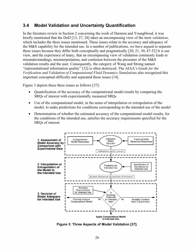
Figure 3 depicts these three issues as follows [37]:

• Quantification of the accuracy of the computational model results by comparing the SRQs of interest with experimentally measured SRQs

• Use of the computational model, in the sense of interpolation or extrapolation of the model, to make predictions for conditions corresponding to the intended use of the model

• Determination of whether the estimated accuracy of the computational model results, for the conditions of the intended use, satisfies the accuracy requirements specified for the SRQs of interest

Figure 3: Three Aspects of Model Validation [37].

27

As depicted in Fig. 3, issue 1 deals with assessing the accuracy of results from the model by comparisons with available experimental data. The assessment could be conducted for the actual system of interest at the actual operating conditions for the intended use of the system, or for simplified elements of the system. However, it is common that these data are not available for the complete system, and as a result, an accuracy assessment of the model is conducted on similar systems, on subsystems, or on components of subsystems. In M&S, we believe that model accuracy should be quantitatively estimated using a validation metric operator [20, 21, 30, 48-51, 53]. This operator computes a difference between the computational results and the experimental results for individual SRQs as a function of the input or control parameters in the validation domain. The operator can also be referred to as a “mismatch” function between the computational results and the experimental results over the multidimensional space of all input parameters. In general, it is a statistical operator because the computational results and the experimental results are not single numbers but distributions of numbers (e.g., cumulative distributions functions) or quantities that are interval valued.

Issue 2 deals with a fundamentally and conceptually different topic, prediction, i.e., foretelling the response of a system under conditions for which the model has not been validated [14]. Prediction can also be thought of as interpolating or extrapolating the model beyond the specific conditions tested in the validation domain to the conditions of the intended use of the model. The important issue here is not the SRQs per se but the estimated total uncertainty in the SRQs of interest as a function of the input parameters and conditions that could exist over the domain of the intended use. The estimated total uncertainty is due to a wide variety of sources depending on the intended use of the model. Some of the uncertainties that commonly occur are as follows:

• Parametric uncertainties in the model for the conditions of the intended use, i.e., uncertainties in parameters in the model that capture random variability in a parameter

• Uncertainties in the validation metric results over the validation domain, e.g., uncertainties due to limited experimental data or poorly characterized experiments (issue 1)

• Uncertainties due to the process of interpolation or extrapolation of the model as a function of the input parameters representing the conditions of the intended use of the model

• Uncertainties in the environments and scenarios for the conditions of the intended use of the model, e.g., an environment in which the system is damaged or compromised is some way.

Predictive uncertainty estimation is a vast field of study far beyond the scope of this report. (See, for example, Refs. [54-57].)

Issue 3 deals with (a) the comparison of the estimated accuracy of the model relative to the accuracy requirements of the model for the domain of the model’s intended use and (b) the decision of adequacy or inadequacy of the model over the domain of the model’s intended use. Although a decision of model adequacy or inadequacy would typically depend on many factors, such as computer resource requirements, we are only referring here to whether the model satisfies or does not satisfy an accuracy requirement. An accuracy requirement may be stated as, “The estimated maximum allowable error for specified SRQs cannot exceed a fixed value over

28

the domain of the model’s intended use.” The estimated error mentioned in the issue 2 discussion will be a function of the input parameters, and the estimated error will be an uncertain quantity. The maximum allowable error over the parameter range of the intended use of the model would typically be an absolute-value quantity or an absolute value for a relative error quantity.

There are two types of “yes” decisions that could occur in issue 3: (a) the estimated error is less than the maximum allowable error over the parameter range of the intended use, and (b) the parameter range of the intended use is modified (restricted) such that the estimated error does not exceed the maximum allowable error.

With this brief discussion of the complex conceptual and practical issues involved in the “encompassing” view of validation, it should be clear that there is a high likelihood for confusion, miscommunication, and misrepresentation of an M&S credibility assessment. As a result, we will adopt more restrictive meanings of certain terms, as follows:

• Model validation will only refer to the assessment of model accuracy, incorporating any uncertainties that may be appropriate. This restricted use of the term “validation” refers to issue 1 above.

• Uncertainty quantification of model predictions will refer to the estimation of total uncertainty in the SRQs of interest as a function of the input parameters and conditions that could exist over the domain of the intended use. This estimation process refers to issue 2.

Issue 3, the decision about whether the model meets the accuracy requirements for its intended use, will not be explicitly dealt with in this discussion of predictive capability. Even though this is an important issue, possibly the most important issue for decision making, it is our view that this issue should not be included in the assessment of predictive capability for two crucial reasons. First, whether or not an M&S result satisfies an M&S accuracy requirement is a programmatic or design decision issue, not a capability issue by itself. Second, the specification of accuracy requirements has proven to be an ethereal and ever-changing goal, depending on such practical application-dependent issues as (1) risk-aversion of the decision maker; (2) design trade-offs between the robustness of interacting subsystems within a complex system; (3) widely varying consequences of the failure of individual subsystems or components as they affect the safety, reliability, and performance in the complete system; and (4) the budget, schedule, resources, and time available for contributing tasks.

Our reason for excluding predictive accuracy requirements parallels that of NASA’s for excluding M&S maturity requirements while assessing M&S maturity, i.e., M&S maturity should be assessed first, then these results could be compared to M&S requirements. This topic is discussed further in Section 5.1.

An important conceptual issue should be stressed here, one that addresses the relationship between the validation of a model and the performance of the engineering system being analyzed. Whether the system of interest, e.g., a component of a nuclear weapon, meets its performance, safety, or reliability requirements is, of course, a completely separate topic from the issues discussed relative to Fig. 3. Simply put, a system model could be accurate, but the system itself could be grossly lacking in performance, safety, or reliability. Whether or not a

29

performance margin is positive (predicted performance exceeds requirements) or negative (predicted performance is less than requirements) is not an issue in predictive capability. Some may say, “It is the most important issue.” We do not disagree with that perspective. However, we argue that assessing the maturity of M&S predictive capability is only one element in assessing the performance, safety, or robustness of an engineering system. This topic is briefly discussed in Section 5.2, Use of the PCMM in Risk-Informed Decision Making.

The assessment of model accuracy, discussed with respect to issue 1, can occur in many different ways. Experimental data that are available on the complete system have been referred to as “data at the top of the validation hierarchy” [14, 16, 20, 21] or as “data for integral effects tests (IETs)” [30]. Here, the term “complete system” means the actual operating system of interest. Experimental data that are available for portions of the complete system, for example, subsystems or components have been characterized as “data at lower levels of the validation hierarchy” [14, 16, 20, 21] or as “data for separate effects tests (SETs)” [30]. An example of a validation hierarchy for an air-breathing hypersonic cruise missile is shown in Fig. 4.

Figure 4: Example of a Validation Hierarchy for a Hypersonic Cruise Missile [20, 21].

One term that has been used extensively is model, though we have not clarified the definition of this term. As is well known, there are many types of models used in M&S. The three major models are conceptual, mathematical, and computational. A conceptual model specifies the

30

physical system and the phenomena of interest, the system environment and its intended use, the physical assumptions that simplify the system and the phenomena of interest, the SRQs of interest, and the accuracy requirements for the SRQs of interest [16, 58, 59]. A mathematical model is derived from the conceptual model, and it is a set of mathematical and logical relations that represent the physical system of interest and its responses to the environment and the ICs of the system [16, 59, 60]. The mathematical model is commonly given by a set of PDEs, integral equations, BCs and ICs, material properties, and excitation equations. The computational model is produced by the numerical implementation of the mathematical model, a process that results in a set of discretized equations and solution algorithms that are then programmed into a computer [16, 59]. Another way to describe the computational model is that it is a mapping of the mathematical model into a software package that, when combined with the proper input, produces simulation results. Sometimes we refer to the computational model simply as the “code.”

When we use the term “model validation” we are actually referring to validation of the mathematical model, even though the simulation results are produced by the computational model. The essence of what is being assessed in validation and the essence of what is making a prediction is embodied in the mathematical model. Viewing model validation as mathematical model validation fundamentally relies on assumptions that the numerical algorithms are reliable, that the computer program is correct, that no human procedural errors have been made in the simulation, and that the numerical solution error is small. The validity of these assumptions must be demonstrated by the activities conducted in code verification and solution verification, as discussed in Sections 3.2 and 3.3, respectively. Section 4.2, Characteristics of PCMM Elements, describes how high scores for model validation and uncertainty quantification cannot be attained unless certain minimum scores are obtained in code verification and solution verification.

3.5 Level of Maturity

Section 2, Review of the Literature, described four methods of ranking the maturity of the various M &S elements. The Harmon and Youngblood [27, 28] five-point maturity ranking scale was dominated by the concepts of credibility, objectivity, and sufficiency of accuracy for the intended use. The Logan and Nitta [29] 10-point scale was dominated by the concepts of completeness, credibility, and sufficiency of accuracy for the intended use. The Pilch et al. [30] four-point scale was dominated by the level of formality, the degree of risk in the decision based on the M&S effort, the importance of the decision to which the M&S effort contributes, and sufficiency of accuracy for the intended use. The NASA [31] four-point scale was dominated by the level of believability, formality, and credibility, excluding the needed adequacy of M&S credibility elements. NASA clearly separated the ideas of credibility assessment of the M&S process from the requirements for a given application of M&S.

Comparing each of the four maturity-ranking methods, we first note that the methods use scales of different magnitude for ranking maturity. We believe, however, that this difference is not fundamentally important. The key difference in our opinion between the four methods is that only the NASA scale explicitly excludes the issue pertaining to adequacy of the maturity assessment; adequacy is addressed after the assessment. We believe this is a major step forward in the interpretability of the assessment of an M&S effort because it segregates the assessed maturity of the process from the required maturity (or credibility) of the result. We expect that

31

some users of the M&S maturity assessment would prefer to have the maturity scale include, or at least imply, the adequacy for the intended use because it would seem to make their decisions easier. However, we strongly believe that the issues of maturity assessment and adequacy assessment should be dealt with independently as much as possible to reduce misunderstandings or misuse of an M&S maturity assessment.

A concept discussed by Pilch et al. [61, 62] for assessing the maturity of each M&S element is based on the risk tolerance of the decision maker. Stated differently, the maturity scale would be given an ordinal ranking based on the risk assumed by the decision maker who uses results generated by the M&S effort. This approach has some appealing features, but it also introduces additional complexities. We mention three difficulties in using a risk-based scale that have practical impact when constructing a maturity scale.

First, risk assessment is commonly, though not correctly, defined to have two components: (1) likelihood of an occurrence and (2) magnitude of the adverse effects of an occurrence. We argue that the estimated likelihood of the occurrence, the identification of possible adverse occurrences, and the estimated magnitude of the adverse consequences are very difficult and costly to determine for complex systems. Consequently, complicated risk assessments commonly involve significant analysis efforts in their own right. Further, combining these complicated risk assessments with the maturity ranking of an M&S effort is difficult to achieve and certainly difficult for anyone to interpret.

Second, the risk tolerance of decision makers or groups of decision makers is a highly variable and difficult attribute to quantify. The original discussion of Pilch et al. correlated the risk-tolerance scale with the increased risk perception of passing from exploratory research to qualification of M&S weapon applications. There are certainly other possibilities for quantifying risk aversion.

Third, the risk tolerance of decision makers inherently involves comparison of the apparent or assessed risk with the requirement of acceptable risk from the perspective of the decision makers. As discussed previously, we reject the concept of incorporating requirements into the maturity assessment. As a result, the maturity ranking scale proposed in this report will not be based on risk or on the risk tolerance of the person or decision maker who uses the information.

Because of these challenges, we take an alternative path in this report and propose a maturity scale with four levels. The levels are based on two fundamental information attributes discussed by Wang and Strong [32]:

• Intrinsic information quality: accuracy, correctness, and objectivity

• Contextual information quality: completeness, amount of information, and level of detail

The use of maturity levels is an attempt to objectively track intellectual artifacts, or evidence, obtained in an assessment of an M&S effort. Any piece of information about the M&S effort can be considered an artifact. As one moves to higher levels of maturity, both the quality and the quantity of intrinsic and contextual information artifacts must increase. The artifacts that are required for the specific elements identified are discussed in Section 4, Proposed Predictive

32

Capability Maturity Model. The general characteristics of the four levels of maturity that apply to all elements follow.

• Level 0 – Little or no assessment of the accuracy or completeness has been made; little or no evidence of maturity; individual judgment and experience only; convenience and expediency are the primary motivators. This level of maturity is commonly appropriate for low-consequence systems, systems with little reliance on M&S, scoping studies, or conceptual design support.

• Level 1 – Some informal assessment of the accuracy and completeness has been made; generalized characterization; some evidence of maturity; some assessment has been made by an internal peer review group. This level of maturity is commonly appropriate for moderate consequence systems, systems with some reliance on M&S, or preliminary design support.

• Level 2 – Some formal assessment of the accuracy and completeness has been made; detailed characterization; significant evidence of maturity; some assessments have been made by an internal peer review group. This level of maturity is commonly appropriate for high-consequence systems, systems with high reliance on M&S, qualification support, or final design support.

• Level 3 – Formal assessment of the accuracy and completeness has been made; precise and accurate characterization; detailed and complete evidence of maturity; essentially all assessments have been made by independent peer-review groups. This level of maturity is commonly appropriate for high-consequence systems in which decision making is fundamentally based on M&S, e.g., where certification or qualification of a system’s performance, safety, and reliability is primarily based on M&S as opposed to being primarily based on complete system testing information.

We have not mentioned the roles or importance of reproducibility, traceability, and documentation of the artifacts. We have excluded these attributes because they do not measure the quality of the information produced; rather, these attributes fundamentally contribute to proof of the existence of the artifacts. We believe that reproducibility, traceability, and documentation of the artifacts are important in an M&S effort, particularly if the effort supports certification of the safety and reliability of high-consequence systems that could affect the public or the environment. The roles of reproducibility, traceability, and documentation of all artifacts produced by computational analyses in risk assessments for nuclear reactor safety, as well as in performance assessments for the Waste Isolation Pilot Plant (WIPP) and the Yucca Mountain Project, are well recognized and mandated by regulatory policy. Not withstanding this experience, our maturity ranking will exclude any proof of existence of the artifacts related to the maturity of the M&S effort.

33

4. Proposed Predictive Capability Maturity Model Using the basic attributes and characteristics described previously, we now describe our proposed Predictive Capability Maturity Model (PCMM). Section 4.1 discusses the purposes and uses of the model. Section 4.2 provides detailed text and tabular descriptions of the elements in the PCMM table, which is a tool designed to facilitate the assessment of maturity of an M&S effort.

4.1 Purpose and Uses of the PCMM

For reasons that will become clear in the discussion that follows, we have divided the four groups discussed in Section 3 into six elements for the PCMM. The four groups in Section 3 were physics modeling fidelity, code verification, solution verification, and model validation and uncertainty. For the PCMM, physics modeling fidelity was divided into two elements: representation and geometric fidelity, and physics and material model fidelity. And model validation and uncertainty was also divided into two elements for the PCMM: model validation, and uncertainty quantification and sensitivity analysis. Thus, the elements that will be used for the PCMM are as follows:

• Representation and geometric fidelity

• Physics and material model fidelity

• Code verification

• Solution verification

• Model validation

• Uncertainty quantification and sensitivity analysis

For each of these elements, maturity is assessed according to the four-level scale described in Section 3.5, Level of Maturity. The contributing elements and the maturity of each element can be thought of as relatively independent measures, or attributes, of predictive capability. Accordingly, the PCMM can be summarized in a table format, where the elements form the rows of the table and the maturity levels (0 through 3) form the columns, as shown in Table 1.

A PCMM assessment consists of evaluating the maturity level of six individual elements and scoring the maturity level of each element. For each level of maturity, there are a set of predefined descriptors that are used to assess the maturity level of a particular element. If an element is characterized by an assessor (an individual who performs the actual assessment of the maturity level for an element) as encompassing the entire set of descriptors at a given level of maturity, the element can be considered to be fully assessed at that level of maturity. An element that is fully assessed at a particular level of maturity will generally be assigned, by the assessor, a score that is equivalent to the maturity level. Thus, for example, if an element was assessed so that it fully met all of the predefined descriptors at maturity level 1, the element would have a score of 1. In preliminary evaluations of the PCMM table over a range of engineering applications, we have commonly found that some, but not all, of the descriptors at a given level

34

Table 1: Table Format for PCMM Assessment

MATURITY

ELEMENT

Maturity Level 0

Maturity Level 1

Maturity Level 2

Maturity Level 3

Representation and Geometric

Fidelity

Physics and Material Model

Fidelity

Code Verification

Solution Verification

Model Validation

Uncertainty Quantification and Sensitivity

Analysis

have been achieved. For example, at maturity level 2, only half the descriptors for a given attribute may have been attained. For this common situation, it has proven useful to give a fractional score for the maturity level instead of strictly assigning an integer score at the lower level of maturity. As a result, noninteger maturity scores expressed in tenths, such as 1.5 for partially achieving level 2, should be considered in assessing the maturity level of each element. In Section 4.2.5 we discuss certain requirements that affect the order in which the individual elements are assessed as well as the scores that can be assigned to certain elements, give scores on other elements. Upon completion of the assessment, the table would have six individual scores, one score per element.

Before presenting additional details about the table constructed for the PCMM, it is appropriate to discuss more clearly the purpose of this table, certain characteristics of the table, and how the results (i.e., scores) from completing this table can be used. Simply stated, the purpose of the table is to assess the level of maturity, at a given point in time, of the key elements in an M&S effort that are directed at an application of interest. As explained in Section 3, the assessment should be conducted, in principle, with little or no regard to any programmatic (or project) requirement for the maturity of the M&S effort. Objectivity, a key ingredient of intrinsic information quality (discussed previously in Section 3.5), increases to the degree that maturity assessment is separated from project maturity requirements.

Table 2 gives an example of a PCMM table after a maturity assessment of an M&S effort has been completed.

35

Table 2: Example of Predictive Capability Maturity Model after Maturity Assessment

MATURITY

ELEMENT

Maturity Level 0

Maturity Level 1

Maturity Level 2

Maturity Level 3

Element Score

Representation and Geometric

Fidelity

Assessed

1

Physics and Material Model

Fidelity

Assessed

2

Code Verification

Assessed 1

Solution Verification

Assessed 0

Model Validation

Assessed 1

Uncertainty Quantification and Sensitivity

Analysis

Assessed

0

For purposes of explanation, consider that all elements in Table 2 were assessed with the scores shown to the right of the table. Then the designator “Assessed” would be placed in the appropriate row and column in the table. Once the assessment has been completed, the set of scores for each element can be compiled. In Table 1, the set of scores completed by the assessor(s) for the six elements is [1, 2, 1, 0, 1, 0].

We believe the type of summary information shown in Table 2 will prove very useful and informative in many environments. Following are some of the experiences we had in our preliminary use of the PCMM table.

• In attempting to conduct a PCMM assessment, we found that the assessors are generally not familiar with many of the concepts in the table. As a result of learning about these concepts, the assessors will greatly broaden and deepen their knowledge of many of the elements that contribute to confidence in M&S.

• Conducting a PCMM assessment and sharing it with interested parties, decision makers, and stakeholders engenders discussions that would not have occurred without such an assessment. This kind of communication is one of the most significant consequences of an M&S maturity assessment in general. An example of a beneficial interaction would be to initiate a conversation with a stakeholder who may not be familiar with any of the contributing elements to M&S and help to educate that stakeholder about the importance of these elements and the results of the assessment.

• PCMM assessments made over a period of time can be used to track the progress of M&S efforts. This is useful for M&S managers, stakeholders (decision makers using the results

36

of the M&S effort), and M&S funding sources to determine progress or value added over time.

A key practical issue in completion of the PCMM table is, who should provide the assessments in the table? We strongly believe that an individual, or a team, that has detailed knowledge of an element should complete that element of the table. These individuals should be very familiar with the elements of the M&S effort and the application of interest. Sometimes, depending on the magnitude of the M&S effort, an M&S project manager is sufficiently familiar with all elements of the table and can complete it in its entirety. The assessed levels in the completed table should represent the actual status of the M&S effort, not some anticipated or future status. In other words, the table should measure the maturity of the actual status at a given point in time, not something that is “nearly” attained or a status that would “look good” in a program review or in a marketing activity.

With the PCMM, we are primarily interested in providing M&S maturity assessment information for an application of interest to program managers, interested stakeholders, and decision makers. We recognize that many other issues enter into risk-informed decision making, some of which are discussed in Section 5.2, Use of PCMM Scores in Risk-Informed Decision Making. Some applications of interest that commonly involve M&S efforts are (a) design or optimization of new systems; (b) modification or optimization of existing systems; and (c) assessment of the performance, safety, or reliability of existing or proposed systems. When we refer to a system, we include any engineered or natural system entity, e.g., subsystems, components, or part of a component. In addition, the specification of a system includes the specification of the environment in which the system must operate, e.g., normal, abnormal, or hostile environments. With the system and environment specified, one can then begin to identify particular aspects of each of the six elements that are important to the M&S effort.

In the nuclear weapons complex, the topic of quantification of margins and uncertainty (QMU) has attained a high level of visibility. Accordingly, some comments should be made about the relationship of the PCMM to QMU [62]. QMU means different things to different people. For the discussion here, we view QMU as a process for predicting the performance of a system and for comparing the predicted performance with the required performance, while including the uncertainty in both the estimated performance and the required performance. Given this interpretation of QMU, we view the PCMM as one of many factors that should be considered in the assessment of the predicted system performance, its estimated uncertainty, and the estimated uncertainty in the difference between the predicted performance and the performance requirement. For example, the PCMM could influence confidence in the estimated margin of the system. We also see situations where the PCMM could alter specifications for the required performance of certain elements of a system. For example, if a requirement for the maximum miss distance of a weapon from a hardened, deeply buried target was specified, M&S could be used to alter the miss distance requirement if more information could be obtained on the characteristics of the target.

An important aspect should be mentioned again concerning the interpretation of scores from a PCMM assessment. Although this aspect was discussed previously in this report, it needs to be stressed and clarified further because it can cause great confusion. We have observed that users of the PCMM commonly interpret an increase in maturity assessment over time to mean that the

37

accuracy of the M&S predictions has improved. This is not necessarily true. Stated differently, many people want to interpret the PCMM scores as a predictive accuracy assessment or, similarly, as a measure of the accuracy of the M&S results. As stressed in Section 3.5, Level of Maturity, the PCMM assesses the maturity of the M&S process elements, not necessarily the accuracy of the M&S results. The accuracy of the M&S results would commonly increase as the PCMM scores improve, but there is not a one-to-one correspondence.

To clarify why this is true, consider an example based on Table 2. As explained previously, the maturity level scores shown in Table 2 are written as the sequence [1, 2, 1, 0, 1, 0] for the six elements. Suppose that the element of uncertainty quantification and sensitivity analysis was improved from a 0 assessment (the last value in the maturity assessment above) to the condition where multiple simulations were obtained and resulted in capturing some of the uncertainties present in the system being analyzed. For example, suppose the uncertainty quantification analysis began to show a large effect due to variability in the strength of welded joints in a component. With this improved uncertainty quantification, suppose the maturity assessment of the PCMM then became [1, 2, 1, 0, 1, 1], i.e., the last value in the sequence changed from 0 to 1. The decision maker would then have more complete information about the system’s uncertainty quantification. The decision maker would then have an estimate of the uncertainty of the SRQs of interest as a function of the variability in weld strength, whereas previously the decision maker may have had no idea of the uncertainty. While the accuracy of the predictions in these hypothetical cases has not changed, the decision maker would now be able to recognize some of the contributing uncertainties to the predicted performance of the system.

4.2 Characteristics of PCMM Elements

A description of each element of the PCMM table is given in Table 3. This table can be used to become familiar with the basic descriptors of each element. Please note that the requirements of the descriptors at each maturity level accumulate as one moves to higher maturity levels within an element. For example, to attain a given maturity level for a given element, the descriptors within the specific element of the table must be satisfied, in addition to all descriptors at the lower levels in that element or row.

A detailed discussion follows for each element of the table.

38

Table 3: General Descriptions for Table Entries of the PCMM

MATURITY

ELEMENT

Maturity Level 0 Low Consequence,

Minimal M&S Impact, e.g. Scoping Studies

Maturity Level 1 Moderate Consequence,

Some M&S Impact, e.g. Design Support

Maturity Level 2 High-Consequence, High M&S Impact,

e.g. Qualification Support

Maturity Level 3 High-Consequence,

Decision-Making Based on M&S, e.g. Qualification or Certification

Representation and Geometric Fidelity What features are neglected because of simplifications or

stylizations?

• Judgment only • Little or no

representational or geometric fidelity for the system and BCs

• Significant simplification or stylization of the system and BCs

• Geometry or representation of major components is defined

• Limited simplification or stylization of major components and BCs

• Geometry or representation is well defined for major components and some minor components

• Some peer review conducted

• Essentially no simplification or stylization of components in the system and BCs

• Geometry or representation of all components is at the detail of “as built”, e.g., gaps, material interfaces, fasteners

• Independent peer review conducted

Physics and Material Model Fidelity

How fundamental are the physics and material models and what is the level of model calibration?

• Judgment only • Model forms are either

unknown or fully empirical

• Few, if any, physics-informed models

• No coupling of models

• Some models are physics based and are calibrated using data from related systems

• Minimal or ad hoc coupling of models

• Physics-based models for all important processes

• Significant calibration needed using separate effects tests (SETs) and integral effects tests (IETs)

• One-way coupling of models • Some peer review conducted

• All models are physics based • Minimal need for calibration using SETs

and IETs • Sound physical basis for extrapolation

and coupling of models • Full, two-way coupling of models • Independent peer review conducted

Code Verification Are algorithm deficiencies,

software errors, and poor SQE practices corrupting the

simulation results?

• Judgment only • Minimal testing of any

software elements • Little or no SQE

procedures specified or followed

• Code is managed by SQE procedures

• Unit and regression testing conducted

• Some comparisons made with benchmarks

• Some algorithms are tested to determine the observed order of numerical convergence

• Some features & capabilities (F&C) are tested with benchmark solutions

• Some peer review conducted

• All important algorithms are tested to determine the observed order of numerical convergence

• All important F&Cs are tested with rigorous benchmark solutions

• Independent peer review conducted

Solution Verification Are numerical solution errors and

human procedural errors corrupting the simulation results?

• Judgment only • Numerical errors have

an unknown or large effect on simulation results

• Numerical effects on relevant SRQs are qualitatively estimated

• Input/output (I/O) verified only by the analysts

• Numerical effects are quantitatively estimated to be small on some SRQs

• I/O independently verified • Some peer review conducted

• Numerical effects are determined to be small on all important SRQs

• Important simulations are independently reproduced

• Independent peer review conducted

Model Validation How carefully is the accuracy of the simulation and experimental

results assessed at various tiers in a validation hierarchy?

• Judgment only • Few, if any,

comparisons with measurements from similar systems or applications

• Quantitative assessment of accuracy of SRQs not directly relevant to the application of interest

• Large or unknown exper-imental uncertainties

• Quantitative assessment of predictive accuracy for some key SRQs from IETs and SETs

• Experimental uncertainties are well characterized for most SETs, but poorly known for IETs

• Some peer review conducted

• Quantitative assessment of predictive accuracy for all important SRQs from IETs and SETs at conditions/geometries directly relevant to the application

• Experimental uncertainties are well characterized for all IETs and SETs

• Independent peer review conducted Uncertainty

Quantification and Sensitivity

Analysis How thoroughly are uncertainties

and sensitivities characterized and propagated?

• Judgment only • Only deterministic

analyses are conducted

• Uncertainties and sensitivities are not addressed

• Aleatory and epistemic (A&E) uncertainties propagated, but without distinction

• Informal sensitivity studies conducted

• Many strong UQ/SA assumptions made

• A&E uncertainties segregated, propagated and identified in SRQs

• Quantitative sensitivity analyses conducted for most parameters

• Numerical propagation errors are estimated and their effect known

• Some strong assumptions made • Some peer review conducted

• A&E uncertainties comprehensively treated and properly interpreted

• Comprehensive sensitivity analyses conducted for parameters and models

• Numerical propagation errors are demonstrated to be small

• No significant UQ/SA assumptions made • Independent peer review conducted

39

4.2.1 Representation and Geometric Fidelity This element is directed primarily toward the level of physical or informational characterization of the system being analyzed or the specification of the geometrical features of the system. For fully empirical and semi-empirical models, there is usually little geometric fidelity, e.g., lumped-mass representations or representations that simply deal with the functionality of system components. For physics-based models that solve PDEs, significant geometric fidelity can be specified that is then used to prescribe the ICs and BCs for such equations. For other computational models, such as electrical circuit or agent-based models, other concepts of representation fidelity are needed. For example, in the case of electrical models, characterization deals with the fidelity of the electrical circuit diagram and level of characterization of the electrical components in the system. For agent-based models, representation fidelity might be the geography over which agents move. Geometric fidelity typically increases as the level of detail of the physical modeling increases. Thus, the lowest level of maturity assesses geometric fidelity based on convenience, simplicity, and the judgment of the computational practitioner. The higher levels of geometric maturity provide increasingly detailed information that is more representative of the “as built” or “real use” geometry; accordingly, levels of stylization of the system and environment decrease. For example, higher levels of detail are typically given in terms of a CAD/CAM file of the geometry, material and surface characteristics, and mechanical assembly of the system. For systems that may be in a state of excessive wear or that may be in abnormal or damaged condition, the specification of the geometry and surface properties can become quite complex and quite uncertain.

General descriptions of the levels of representation and geometric fidelity follow:

• Level 0: Simplicity, convenience, and functional operation of the system dominate the fidelity of the representation and the geometry for the system being analyzed. There is heavy reliance on judgment and experience, with little or no expectation or quantification of representation and geometric fidelity.

• Level 1: Quantitative specifications are applied to describe the geometry of the major components of the system being analyzed. Much of the real system remains stylized or ignored, e.g., gaps in systems, changes in materials, and surface finish.

• Level 2: Quantitative specifications are applied to replicate the geometric fidelity of most of the components of the real system. Little of the real system remains stylized or ignored. For example, important imperfections due to system assembly or defects due to wear or damage in the system are included. A level of peer review, such as an informal review or an internal review, of the model representation and geometric fidelity has been conducted.

• Level 3: The geometric representation in the model is “as built” or “as existing,” meaning that no aspect of the geometry of the modeled real system is missing, down to scales that are determined to be relevant to the level of physical modeling chosen. An example is a complete CAD/CAM model for the real system as assembled and meshed for the computational model with virtually no approximations or simplifications included. Independent peer review of the model representation and geometric fidelity has been conducted, e.g., formal review by the M&S effort customer or by reviewers external to the organization conducting the M&S.

40

4.2.2 Physics and Material Model Fidelity

This attribute primarily addresses the following:

• The degree that models are physics based

• The degree to which the models are calibrated

• The physics fidelity basis with which the models are being extrapolated from their validation and calibration database to the conditions of the application of interest

• The quality and degree of coupling the multiphysics effects that exist in the application of interest

As discussed in Section 3.1, Physics Modeling Fidelity, models typically range from fully empirical to physics based:

• Fully empirical – The model is based entirely on statistical fits of experimental data.

• Semi-empirical – The model conserves mass, momentum, and energy, but it fundamentally relies on calibration of important parameters.

• Physics based – An example is an electrical circuit model coupled to a physics-based model of the electrical currents generated by circuit wiring exposed to an electromagnetic environment.

Generally, as the fidelity of the model increases, the model is increasingly more able to provide physics-based explanatory power for the particular physical phenomenon of interest. Within the broad class of physics-based models, there are important distinctions in the degree to which the model is calibrated. For example, does the model require recalibration even if there are relatively small changes in the system design or small changes in the system environment? Alternately, does the model require calibration only at lower levels in the validation hierarchy, i.e., separate effects tests (SETs), in order to yield accurate predictions? Or, does the model also require calibration or recalibration at higher levels of the validation hierarchy, i.e., integral effects tests (IETs), to attain accurate predictions? For two models yielding the same level of agreement with experimental data, one model calibrated with SETs and one model calibrated with IETs, the model that requires calibration with the SETs has more predictive capability than does the model that requires calibration with the IETs. The maturity ranking and understanding of the coupled physics effects and their importance should be closely related to the development and use of a Phenomena Identification and Ranking Table (PIRT) [49, 63].

General descriptions of the various levels of physics and material model fidelity follow:

• Level 0: The model is fully empirical, or the model form is not known. There is little or no coupling of models representing multiple functional elements of the system, and the coupling that does exist is not physics based. Confidence in the model is strictly based on the judgment and experience of the practitioner.

• Level 1: The model is semi-empirical in the sense that portions of the modeling are physics based; however, important features, capabilities, or parameters in the model are

41

calibrated using data from very closely related physical systems. The coupling of functional elements or components is minimal, or ad hoc, and not physics based.

• Level 2: All important physical process models and material models are physics based. Calibration of important model parameters is necessary, using data from SETs and IETs. All model calibration procedures are implemented on the model input parameters, not on the SRQs. Important physical processes are coupled using physics-based models with couplings in one direction. Some level of peer review, such as an informal review or an internal review, of the physics and material models has been conducted.

• Level 3: All models are physics based with minimal need for calibration using SETs and IETs. Where extrapolation of these models is required, the extrapolation is based on well-understood and well-accepted physical principles. All physical processes are coupled in terms of physics-based models with two-way coupling and physical process effects on physical and material parameters, BCs, geometry, ICs, and forcing functions. Independent peer review of the physics and material models has been conducted, e.g., formal review by the M&S effort customer or by reviewers external to the organization conducting the M&S.

4.2.3 Code Verification

This attribute focuses on the following:

• Correctness and fidelity of the numerical algorithms used in the code relative to the mathematical model, e.g., the PDE model

• Correctness of source code

• Configuration management, control, and testing of the software through SQE practices

The correctness and fidelity of the numerical algorithms and the correctness of the source code are primarily determined by conducting various types of tests on the code. The primary type of test is to compare the numerical solution results from the code with highly accurate solutions, which are usually referred to as benchmark solutions [37]. The most rigorous benchmark solutions are manufactured solutions and analytical solutions [15, 33]. Comparisons between the code and the benchmark solutions can result in error measures between the code and the SRQs, or these comparisons can yield a calculation of the observed order of convergence of the numerical algorithm in the code being tested.

The maturity of the SQE practices should measure the scope and rigor of configuration management and software control.

General descriptions of the levels of code verification are as follows:

• Level 0: Code verification is based almost entirely on the judgment and experience of the computational practitioners involved. There is little or no formal verification testing of the software elements. Little or no SQE practices are defined and practiced in the implementation, management, and use of the code.

42

• Level 1: Most associated software is implemented and managed with formal SQE practices. Unit and regression testing of the software is conducted regularly with a high percentage of line coverage attained. Verification test suites using benchmark solutions are minimal, and only error measures are obtained in some SRQs.

• Level 2: All associated software is implemented and managed with formal SQE practices. Verification test suites are formally defined and systematically applied using benchmark solutions to compute the observed order of convergence of some numerical algorithms. Some features and capabilities (F&Cs), such as complex geometries, mesh generation, physics, and material models, have been tested with benchmark solutions. Some level of peer review, such as an informal review or an internal review, of the code verification has been conducted.

• Level 3: All important algorithms have been tested using rigorous benchmark solutions to compute the observed order of convergence. All important features and capabilities (F&Cs), such as two-way coupling of multiphysics processes, have been tested with rigorous benchmark solutions. Independent peer review of code verification has been conducted, e.g., formal review by the M&S effort customer or by reviewers external to the organization conducting the M&S.

4.2.4 Solution Verification

This attribute deals with assessment of the following:

• Numerical solution errors in the computed results

• Confidence in the computational results as they may be affected by human errors

Rigor and numerical solution reliability are the dominant components of the assessment of this element. Numerical solution errors are any errors due to mapping the mathematical model to the discretized model and any errors due to solution of the discretized model on a computer. Of concern in this element are numerical solution errors due to spatial and temporal discretization of the PDEs or integral equations and the iterative solution error due to a linearized solution approach to a set of nonlinear discretized equations. Additional numerical solution errors that should be addressed are the potential detrimental effects of numerical parameters in solution algorithms; errors due to approximate techniques used to solve nondeterministic systems, e.g., error due to a small number of samples used in a Monte Carlo sampling method; and round-off error due to finite precision on a computer. Human errors (mistakes) are also a concern in the assessment of this element. Human errors are any errors made in (1) preparing and assembling the elements of the computational model, (2) executing the computational solution, and (3) postprocessing, preparing, or interpreting the computational results.

General descriptions of the levels of solution verification are as follows:

• Level 0: No formal attempt is made to assess any of the possible sources of numerical error. Any statement about the impact of numerical error is based purely on the judgment and experience of the computational practitioner. No assessment about the correctness of software inputs or outputs has been conducted.

43

• Level 1: Some kind of formal method is used to assess the influence of numerical errors on some SRQs. This could include a posteriori error estimation of global norms, iterative convergence studies, or sensitivity studies to determine how sensitive certain SRQs are to changes in mesh or temporal discretization. A formal effort is made by the computational practitioners to check the correctness of input/output (I/O) data.

• Level 2: Quantitative error estimation methods are used to estimate numerical errors on some SRQs, and these estimates show that the errors are small for some conditions of the application of interest. I/O quantities have been verified by knowledgeable computational practitioners who have some level of independence from the M&S effort. Some level of peer review, such as an informal review or an internal review, of the solution verification activities has been conducted.

• Level 3: Quantitative error estimation methods are used to estimate numerical errors on all important SRQs, and these estimates show that the errors are small over the entire range of conditions for the application of interest. Important computational simulations are reproduced, using the same software, by independent computational practitioners. Independent peer review of solution verification activities has been conducted, e.g., formal review by the M&S effort customer or by reviewers external to the organization conducting the M&S.

A subtle, but important, point should be stressed regarding the maturity levels of solution verification. In Section 3.5, Level of Maturity, and Section 4.1, Purpose and Uses of the PCMM, we stressed that higher levels of maturity do not necessarily imply higher levels of accuracy of the M&S results. However, in the descriptions of maturity levels just given it is apparent that higher levels level of maturity require increased solution accuracy. This apparent dichotomy is resolved by understanding that increased numerical solution accuracy is necessary to gain more confidence in the fidelity of the mapping of the mathematical model to the solution of the discrete model. We are not necessarily gaining confidence in the comparison of the computational results with experimental data. In other words, we require increased correctness and accuracy of the numerical solution, including code verification, so that when we compare computational results and experimental results we are confident that we are indeed comparing the physics of the mathematical model with nature’s reflection of reality in experimental measurements. The user of the M&S results should be presented quantitative information concerning how well the numerical results represent the physics in the PDE model, as opposed to a contaminated mixture of physics and numerical error. If we cannot have confidence in what we believe we are comparing, then we are dealing with a convolved mixture of physics modeling, physics modeling approximations (error), and numerical error, in which no bases for confidence can be made. We will see in Section 4.2.5 that more accurate comparisons between the computational results and the experimental measurements are not required to achieve higher maturity levels in model validation.

4.2.5 Model Validation

This attribute focuses on the following:

• Thoroughness and precision of the accuracy assessment of the computational results relative to the experimental measurements

44

• Completeness and precision of the characterization of the experimental conditions and measurements

• Relevancy of the experimental conditions, physical hardware, and measurements in the validation experiments compared to the application of interest

As discussed in Section 3.4, Model Validation and Uncertainty Quantification, and Section 4.1, Purpose and Uses of the PCMM, the focus of model validation is on the precision and completeness of the process of the model accuracy assessment, not on the accuracy of the computational model itself. By “precision” of validation we mean, (1) how carefully and accurately are the experimental uncertainties estimated? and (2) how well understood and quantified are all of the conditions of the experiment that are required as inputs for simulation by the computational model? By “completeness” of validation we mean, how well do the conditions (geometry, BCs, ICs, and forcing functions) and actual physical hardware of the validation experiments conducted relate to the actual conditions and hardware of the application of interest?

For SETs, it is expected that there will be many dissimilarities between the SET experiments and the actual application of interest. For IETs, however, there should be a close relationship between the IET experiments and the application of interest, particularly with respect to the experimental hardware and the coupled physical phenomena occurring in each. For a more complete discussion of the concepts behind SETs, IETs, and the construction of a validation hierarchy, see Refs. [14, 16, 20, 21, 30, 49].

As discussed in Section 3.4, Model Validation and Uncertainty Quantification, the correctness and credibility of model validation fundamentally relies on assumptions that the numerical algorithms are reliable, that the computer program is correct, that no human procedural errors have been made in the simulation, and that the numerical solution error is small. These are major assumptions that we, and many others in M&S, have discovered are commonly unfounded. Consequently, to properly inform the user of the information in the PCMM table about the veracity of these assumptions, we require that the maturity level of the elements model validation and uncertainty quantification and sensitivity analysis can be no higher than two levels above the maturity levels of the minimum of code verification and solution verification. This requirement places further restrictions on conducting the PCMM assessment and means that the maturity levels of code verification and solution verification must be assessed before the maturity levels of model validation and of uncertainty quantification and sensitivity analysis are assessed. As an example of the dependencies between elements, assume that, as discussed in Table 2, code verification and solution verification were at levels 1 and 0, respectively. Consequently, the maximum maturity level that the model validation element and the uncertainty quantification and sensitivity analysis element could be is level 2. Stated differently, if either code verification or solution verification has a maturity level of 0, then both the model validation element and the uncertainty quantification and sensitivity analysis element can have a maximum maturity level of 2, even if the assessor(s) were to independently judge either or both of these elements at a level higher than 2.

General descriptions of the various levels of model validation are as follows:

45

• Level 0: Accuracy assessment of the model is based almost entirely on judgment and experience. Few, if any, comparisons have been made between computational results and experimental measurements of similar systems of interest.

• Level 1: Limited quantitative comparisons are made between computational results and experimental results. Either comparisons for SRQs have been made that are not directly relevant to the application of interest or the experimental conditions are not directly relevant to the application of interest. Experimental uncertainties, either in the SRQs and/or in the characterization of the conditions of the experiment, are largely undetermined or based on experience.

• Level 2: Quantitative comparisons between computational results and experimental results have been made for some key SRQs from SET experiments and limited IET experiments. Experimental uncertainties are well characterized (a) for most SRQs of interest and (b) for experimental conditions for the SETs conducted; however, the experimental uncertainties are not well characterized for the IETs. Some level of peer review, such as an informal review or an internal review, of the model validation activities has been conducted.

• Level 3: Quantitative comparisons between computational and experimental results have been made for all important SRQs from an extensive database of both SET and IET experiments. The conditions of the SETs should be relevant to the application of interest; and the conditions, hardware, and coupled physics of the IETs should be very similar to the application of interest. Some of the SET computational predictions and most of the IET predictions should be “blind.” Experimental uncertainties and conditions are well characterized for SRQs in both the SET and IET experiments. Independent peer review of the model validation activities has been conducted, e.g., formal review by the M&S effort customer or by reviewers external to the organization conducting the M&S.

4.2.6 Uncertainty Quantification and Sensitivity Analysis

This attribute focuses on the following:

• Thoroughness and soundness of the uncertainty quantification effort, including identification and characterization of all plausible sources of uncertainty

• Accuracy and correctness of propagating uncertainties through a computational model and interpreting uncertainties in the SRQs of interest

• Thoroughness and precision of a sensitivity analysis to determine the most important contributors to uncertainty in system responses

Recognition of uncertainties refers to the activity of identifying and understanding all possible uncertainties within the system of interest, such as parametric uncertainty and uncertainties in the geometry, BCs, forcing functions, or environmental conditions. Characterization of model predictive uncertainty primarily deals with the proper estimation and representation of all uncertainties that could exist as part of the prediction for the system of interest. A key aspect of characterization, appreciated for almost two decades by the risk-assessment community, is the segregation of uncertainties into aleatory and epistemic elements [54-56, 64]. Aleatory

46

uncertainty is uncertainty due to inherent variation associated with the system of interest or the environment. Aleatory uncertainty is also referred to as variability, irreducible uncertainty, stochastic uncertainty, and uncertainty due to chance. Epistemic uncertainty is uncertainty due to lack of knowledge with respect to any phase of the M&S process for the system of interest or the environment. For example, a parameter that is a purely epistemic uncertainty is characterized by a situation for which there exists a single, correct, or true value, but the value is not known precisely. Epistemic uncertainty is also referred to as reducible uncertainty and sometimes as subjective uncertainty.

Propagating uncertainty addresses two questions: How are input uncertainties propagated through the model? and How are uncertainties in the model itself estimated? Input uncertainty refers to any uncertainty in any input quantity for the model, including parameters, BCs, forcing functions, environments, and scenarios. Input uncertainties can be purely aleatory, purely epistemic, or a mixture of aleatory and epistemic. Uncertainties in the model itself can be due to lack of knowledge of the physical processes or due to approximations made that eliminate certain aspects of the physical processes of interest. Model form uncertainty is a purely epistemic uncertainty. As a result, the mathematical model may not be completely reliable. Model form uncertainty can sometimes be estimated by using alternate or competing models to represent the same physical process. This approach can be effective if a lower-fidelity model is compared to a higher-fidelity, more reliable model of the physics. The higher-fidelity model, however, could be so prohibitively expensive from a computational resources perspective that it could not be used extensively in the uncertainty quantification analysis.

A sensitivity analysis provides additional important information to the user of the computational simulation analysis beyond what is typically considered a part of an uncertainty quantification analysis [65, 66]. A sensitivity analysis is typically directed at two closely related goals. First, one may be interested in determining which computational simulation inputs have the largest effect, either locally or globally, on a particular SRQ or group of SRQs. The information obtained from the first goal is commonly used for system design and optimization, as well as for determination of the most advantageous operational conditions for maximizing system performance. Second, one may be interested in determining which uncertain simulation inputs produce the largest change in uncertainty of a particular SRQ or group of SRQs. The information from this second goal may be used, for example, to determine which manufacturing variabilities contribute most to variability in certain SRQs, or to determine what physical experiments should be conducted to most reduce the epistemic uncertainty that is due to poorly understood coupled-physics phenomena.

As discussed previously in Section 4.2.5, Model Validation, the maturity level of the model validation element and the uncertainty quantification and sensitivity analysis element can be no higher than two levels above the maturity levels of the minimum of code verification and solution verification.

General descriptions of the various levels of uncertainty quantification and sensitivity analysis are as follows:

47

• Level 0: Judgment and experience are dominant forms of uncertainty assessment. Only deterministic analyses were conducted for the system of interest. Informal “spot checks” or “what if” studies for various conditions were conducted to determine their effect.

• Level 1: Uncertainties in the system of interest are identified, represented, and propagated through the computational model, but they are not segregated with respect to whether the uncertainties are aleatory or epistemic. Sensitivity of some system responses to some system uncertainties and environmental condition uncertainties was investigated, but the sensitivity analysis was primarily informal or exploratory rather than systematic. Many strong assumptions are made with respect to the uncertainty quantification/sensitivity analysis (UQ/SA); for example, most probability density functions are characterized as Gaussian, and uncertain parameters are considered to be independent of all other parameters.

• Level 2: Uncertainties in the system of interest are characterized as either aleatory and epistemic. The uncertainties are propagated through the computational model, while their character is kept segregated both in the input and in the SRQs. Quantitative sensitivity analyses were conducted for most system parameters, while segregating aleatory and epistemic uncertainties. Numerical approximation or sampling errors due to propagation of uncertainties through the model are estimated, and the effect of these errors on the UQ/SA results is understood. Some strong UQ/SA assumptions were made, but qualitative results suggest that the effect of these assumptions is not significant. Some level of peer review, such as an informal review or an internal review, of the uncertainty quantification and sensitivity analyses has been conducted.

• Level 3: Aleatory and epistemic uncertainties are comprehensively treated, and their segregation in the interpretation of the results is strictly maintained. Detailed investigations were conducted to determine the effect of uncertainty introduced due to model extrapolations, if required, to the conditions of the system of interest. A comprehensive sensitivity analysis was conducted for both parametric uncertainty and model form uncertainty. Numerical approximation or sampling errors due to propagation of uncertainties through the model are carefully estimated, and their effect on the UQ/SA results is demonstrated to be small. No significant UQ/SA assumptions were made. Independent peer review of uncertainty quantification and sensitivity analyses have been conducted, e.g., formal review by the M&S effort customer or by reviewers external to the organization conducting the M&S.

48

5. Additional Uses of the Predictive Capability Maturity Model

In this section, we suggest additional ways that the PCMM can be used and propose a method for the aggregation of scores in the PCMM table should that kind of information be desired. We also point out that the PCMM is only one of many factors that contribute to risk-informed decision making.

5.1 Requirements for Modeling and Simulation Maturity

After an objective assessment of M&S maturity has been made using the PCMM table, the completed PCMM table, as described in Section 4, can be used to specify the project maturity requirements for each element in the table. Six project maturity requirements can be specified, one for each element in the table. Project maturity requirements may be a result of, for example, system qualification or regulatory requirements, or they may simply be progress requirements for the development of an M&S capability. For this exercise, the essential question to ask for each element is, what should the appropriate level of maturity be for my intended use of the M&S activity? For example, a given element in the table has been assessed at a maturity level of 2. Is that an appropriate level for this project or should it be at a higher level? Although we have not discussed this issue, it is obvious that the costs, both in terms of time and resources, increase significantly as higher levels of maturity are attained. To determine the project maturity requirements, one uses the same descriptors in Table 3 that were used to complete the PCMM table in Section 4. For this second pass using Table 3, we consider the descriptors to be project maturity requirements.

Table 4 depicts the results of specifying project maturity requirements for each of the assessed elements discussed in Section 4. The designator “Required” is used to indicate the project maturity requirement for each element. The scores for the project maturity requirements in this example are [2, 2, 1, 2, 2, 3].

As can be seen in Table 4, the values are color coded and have the following meanings:

• Green – The assessment meets or exceeds the requirement.

• Yellow – The assessment does not meet the requirement by one level or less.

• Pink – The assessment does not meet the requirement by two levels or less.

• Red – The assessment does not meet the requirement by three levels or less.

49

Table 4: Example of PCMM Table Assessment and Project Maturity Requirements

MATURITY

ELEMENT

Maturity Level 0

Maturity Level 1

Maturity Level 2

Maturity Level 3

Representation and Geometric

Fidelity

Assessed

Required

Physics and Material Model

Fidelity

Assessed

Required

Code Verification

Assessed

Required

Solution Verification

Assessed Required

Model Validation

Assessed Required

Uncertainty Quantification and Sensitivity

Analysis

Assessed

Required

Some examples of the useful benefits of comparisons of M&S maturity and M&S project maturity requirements, as shown in Table 4, follow.

• To construct Table 4, one must have already addressed the question, What are the project requirements for M&S maturity? In our experience, answering this question has proven difficult but quite useful in its own right. If this question is asked, we have found that it initiates conversations not only within the M&S customer’s organization (typically engineering design groups or decision makers) but also between the M&S developer and customer. We have found that this conversation is particularly important when the M&S customer is not the source of funding for the M&S effort.

• Table 4 can be used as a project management tool to adjust resources for elements that are lagging in their progress to meet project schedule requirements. Note that some elements do not depend solely on computational or software issues. For example, the model validation element depends very heavily on capabilities and progress in experimental activities. In the ASC program, we have found that one of the most common and damaging difficulties is the technical and/or scheduling disconnection between the computational and experimental activities in validation.

50

5.2 Aggregation of PCMM Scores

In Section 4, the description of the PCMM focused on the use of M&S for a particular engineering application. Situations can exist where PCMM scores will need to be aggregated into one score, such as the following:

• Suppose one has obtained a set of scores for multiple subsystems within a system, each subsystem represented by six scores. The desire is to aggregate all of the scores for the multiple subsystems into a single score for all of the subsystems. Note that one may have the same aggregation request for any tier in the validation hierarchy.

• Suppose one has obtained a set of scores for multiple systems of different design, and each system is represented by six scores. The desire is to aggregate all of the scores for the multiple systems into one score that would represent, in some sense, a single score for the collection of systems.

Although we recognize that arguments may be made to compute PCMM aggregate scores, we strongly recommend that this not be done. The score assessed for each of the six M&S elements is an ordinal scale—the four levels of maturity constitute a total order because each pair of levels can be simply ordered. However, the six M&S elements cannot be collectively ordered in any way; they are apples and oranges. Each element is important and conceptually independent from each other element. If one argues that an average maturity of an M&S effort could be computed by simply taking the arithmetic mean of each of the six elements, the average value would have little meaning. The argument for using the average value would be analogous to someone claiming to compute the breaking strength of a chain by averaging the strength of each link in the chain.

Even though we argue against any type of aggregation method, history has clearly shown that pressure to condense information for decision makers can be irresistible. Given this reality, we recommend a simple procedure that would aid in maintaining some of the key information in the individual PCMM scores. We recommend that a set of three scores always be computed and presented to the user of the PCMM when any aggregation of PCMM scores is computed. The scores consist of the minimum over all of the elements being aggregated, the average of all the elements, and the maximum of all the elements. This aggregation triple can be written as:

PCMM! = min

i=1,2,"n

PCMMi,1

nPCMM

i, maxi=1,2,"n

PCMMi

i=1

n

!"

#$

%

&' (1)

where n is the total number of individual PCMM scores that are being aggregated. We believe that keeping the worst score of all aggregated scores will call attention to the situation so that the decision maker can pursue the issue in more depth if desired.

As an example, suppose that a system was made up of four subsystems. Assume each subsystem was assessed using the PCMM table discussed above, with the following result:

51

PCMMsubsystem1 =

1

1.5

1

0

0.5

1

!

"

#######

$

%

&&&&&&&

, PCMMsubsystem2 =

1.5

1

0

0.5

1.5

0

!

"

#######

$

%

&&&&&&&

, PCMMsubsystem3 =

2

1.5

0.5

1

1.5

1

!

"

#######

$

%

&&&&&&&

, PCMMsubsystem4 =

2

2

1

0.5

1.5

1.5

!

"

#######

$

%

&&&&&&&

(2)

Using Eqs. (1) and (2), we compute the PCMM aggregate triple:

PCMM! = 0.0,1.1,2.0[ ] (3)

Our example demonstrates what we have observed in preliminary use of the PCMM: there is commonly a very wide range of scores uncovered in assessments.

5.3 Use of the PCMM in Risk-Informed Decision Making We have proposed that the PCMM should be narrowly focused so that it can be properly understood and correctly used by computational practitioners, experimentalists, project managers, decision makers, and policy makers. In Section 4.1, Purpose of the Predictive Capability Maturity Model, and Section 5.1, Requirements for Modeling and Simulation Maturity, we suggested some ways in which the PCMM could be used to assess progress, used as a project planning tool for both M&S and experimental activities, and used by consumers of M&S information. In the larger context, however, the PCMM is only one factor that contributes to risk-informed decision making for engineering systems. Figure 5 depicts a number of factors that could affect the risk-informed decision making for an engineering system.

Figure 5: Factors Influencing Risk-informed Decision Making.

52

Figure 5 divides the factors into two major groups: technical issues and programmatic issues. Although not all factors are shown, it is seen that a number of diverse and complex factors are important in decision making. Sometimes individual technical factors are characterized fairly well. For example, required system performance and predicted system performance, say, for system reliability in normal operating conditions, might be mathematically characterized as a precisely known probability distribution. However, most of the factors in Fig. 5, particularly programmatic issues, are not characterized well, or at all. For example, it is commonly very difficult to estimate the consequences of poor system reliability on financial liability and future business opportunities. As depicted, there are interactions and trade-offs between the two groups of issues and within each group. Managers and decision makers must weigh the importance all factors, try to understand the complex interactions of factors, and decide on the trade-offs that must be made to optimize their view of “success.” Of course, “success” can mean widely varying things to the various participants and stakeholders involved. Our purpose in constructing and discussing Fig. 5 is to make it clear how the PCMM is but one factor in a complex set of factors. We have argued in this report that the assessment of M&S maturity is a relatively new factor that should be explicitly included in risk-informed decision making. In addition, we have argued that the assessment should be clearly separated from other important factors in decision making. If this is not done, there will be, at best, a convolution of factors causing confusion and miscommunication and, at worst, a contortion of factors intended to satisfy various agendas of individuals and organizations involved.

53

References 1. NRC, Severe Accident Risks: An Assessment for Five U.S. Nuclear Power Plants. 1990,

U.S. Nuclear Regulatory Commission, Office of Nuclear Regulatory Research, Division of Systems Research, NUREG-1150.

2. Breeding, R.J., J.C. Helton, E.D. Gorham, and F.T. Harper, Summary Description of the Methods used in the Probabilistic Risk Assessments for NUREG-1150. Nuclear Engineering and Design, 1992, 135, p. 1-27.

3. Helton, J.C. and R.J. Breeding, Calculation of Reactor Accident Safety Goals. Reliability Engineering and System Safety, 1993, 39(2), p. 129-158.

4. Helton, J.C., Treatment of Uncertainty in Performance Assessments for Complex Systems. Risk Analysis, 1994, 14(4), p. 483-511.

5. Helton, J.C., D.R. Anderson, M.G. Marietta, and R.P. Rechard, Performance Assessment for the Waste Isolation Pilot Plant: From Regulation to Calculation for 40 CFR 191.13. Operations Research, 1997, 45(2), p. 157-177.

6. Helton, J.C., D.R. Anderson, G. Basabilvazo, H.-N. Jow, and M.G. Marietta, Conceptual structure of the 1996 performance assessment for the Waste Isolation Pilot Plant. Reliability Engineering and System Safety, 2000, 69(1-3), p. 151-165.

7. Helton, J.C., D.R. Anderson, G. Basabilvazo, H.N. Jow, and M.G. Marietta, Summary Discussion of the 1996 Performance Assessment for the Waste Isolation Pilot Plant. Reliability Engineering and System Safety, 2000, 69(1-3), p. 437-451.

8. West, M., Real Process Improvement Using the CMMI. 2004, Boca Raton, FL: CRC Press.

9. Ahern, D.M., A. Clouse, and R. Turner, CMMI Distilled: A Practical Introdution to Integrated Process Improvement. 2nd ed. 2005, Boston, MA: Addison-Wesley.

10. Garcia, S. and R. Turner, CMMI Survival Guide: Just Enough Process Improvement. 2006, Boston, MA: Addison-Wesley.

11. Chrissis, M.B., M. Konrad, and S. Shrum, CMMI: Guidlines for Process Integration and Product Improvement. 2nd ed. 2007, Boston, MA: Addison-Wesley.

12. SEI. Software Engineering Institute: Capability Maturity Model Integration. 2006, available from: http://www.sei.cmu.edu/cmmi/.

13. DoD, DoD Instruction 5000.61: Modeling and Simulation (M&S) Verification, Validation, and Accreditation (VV&A). 1996, Defense Modeling and Simulation Office, Office of the Director of Defense Research and Engineering.

14. AIAA, Guide for the Verification and Validation of Computational Fluid Dynamics Simulations. 1998, American Institute of Aeronautics and Astronautics, AIAA-G-077-1998.

15. Roache, P.J., Verification and Validation in Computational Science and Engineering. 1998, Albuquerque, NM: Hermosa Publishers.

16. ASME, Guide for Verification and Validation in Computational Solid Mechanics. 2006, American Society of Mechanical Engineers, ASME V&V 10-2006.

17. Soudah, J., S. Doebling, J. Sefcik, M. Pilch, and T. Trucano, ASC V&V Program Strategy: Toward a Predictive Enterprise. 2006, National Nuclear Security Administration, in preparation.

54

18. Oberkampf, W.L. A Proposed Framework for Computational Fluid Dynamics Code Calibration/Validation. 18th AIAA Aerospace Ground Testing Conference, 1994, Colorado Springs, CO, AIAA Paper 94-2540.

19. Mehta, U.B. Guide to Credible Computational Fluid Dynamics Simulations. 26th AIAA Fluid Dynamics Conference, 1995, San Diego, CA, AIAA Paper 95-2225.

20. Oberkampf, W.L. and T.G. Trucano, Verification and Validation in Computational Fluid Dynamics. Progress in Aerospace Sciences, 2002, 38(3), p. 209-272.

21. Oberkampf, W.L., T.G. Trucano, and C. Hirsch, Verification, Validation, and Predictive Capability in Computational Engineering and Physics. Applied Mechanics Reviews, 2004, 57(5), p. 345-384.

22. Mankins, J.C., Technology Readiness Levels. 1995, National Aeronautics and Space Administration, Advanced Concepts Office, Office of Space Access and Technology.

23. GAO, Best Practices: Better Management of Technology Development Can Improve Weapon System Outcomes. 1999, U. S. Government Accounting Office, GAO/NSIAD-99-162.

24. DoD, Technology Readiness Assessment (TRA) Deskbook. 2005, Department of Defense.

25. Smith, J., An Alternative to Technology Readiness Levels for Non-Developmental Item (NDI) Software. 2004, Carnegie Mellon, Software Engineering Institute, CMU/SEI-2004-TR-013, ESC-TR-2004-013.

26. Clay, R.L., S.J. Marburger, M.S. Shneider, and T.G. Trucano, Modeling and Simulation Technology Readiness Levels. 2007, Sandia National Laboratories, SAND2007-0570.

27. Harmon, S.Y. and S.M. Youngblood. A Proposed Model for Simulation Validation Process Maturity. Simulation Interoperabiity Workshop, 2003, Paper No. 03S-SIW-127.

28. Harmon, S.Y. and S.M. Youngblood, A Proposed Model for Simulation Validation Process Maturity. The Journal of Defense Modeling and Simulation, 2005, 2(4), p. 179-190.

29. Logan, R.W. and C.K. Nitta. Validation, Uncertainty, and Quantitative Reliability at Confidence (QRC). 41st AIAA Aerospace Sciences Meeting and Exhibit, 2003, Reno, NV, AIAA Paper 2003-1337.

30. Pilch, M., T.G. Trucano, D.E. Peercy, A.L. Hodges, and G.K. Froehlich, Concepts for Stockpile Computing. 2004, Sandia National Laboratories, SAND2004-2479 (Restricted Distribution, Official Use Only).

31. NASA, Interim NASA Technical Standard for Models and Simulations. 2006, National Aeronautics and Space Administration, NASA-STD-(I)-7009.

32. Wang, R.Y. and D.M. Strong, Beyond Accuracy: What Data Quality Means to Data Consumers. Journal of Management Information Systems, 1996, 12(4), p. 5-34.

33. Knupp, P. and K. Salari, Verification of Computer Codes in Computational Science and Engineering. 2002, Boca Raton, FL: Chapman & Hall/CRC.

34. Karolak, D.W., Software Engineering Risk Management. 1996, Los Alamitos, CA: IEEE Computer Society Press.

35. Rakitin, S.R., Software Verification and Validation. 1997, Boston, MA: Artech House. 36. Tian, J., Software Quality Engineering: Testing, Quality Assurance, and Quantifiable

Improvement. 2005: Wiley-IEEE Computer Society Press. 37. Oberkampf, W.L. and T.G. Trucano, Verification and Validation Benchmarks. 2007,

Sandia National Laboratories, SAND2007-0853.

55

38. Ferziger, J.H. and M. Peric, Computational Methods for Fluid Dynamics. 1996, New York: Springer-Verlag.

39. Hirsch, C., Numerical Computation of Internal and External Flows: Vol. 1: Fundamentals of Numerical Discretization. 1988, New York: John Wiley.

40. Hirsch, C., Numerical Computation of Internal and External Flows: Vol. 2: Computational Methods for Inviscid and Viscous Flows. 1990, New York: John Wiley.

41. Oden, J.T., Error Estimation and Control in Computational Fluid Dynamics. in The Mathematics of Finite Elements and Applications, J.R. Whiteman, (Ed.), 1993, John Wiley: New York. p. 1-23.

42. Morton, K.W., Numerical Solution of Convection-Diffusion Problems. 1996, Boca Raton, FL: CRC Press.

43. Laney, C.B., Computational Gasdynamics. 1998, Cambridge, U.K.: Cambridge University Press.

44. Ainsworth, M. and J.T. Oden, A Posteriori Error Estimation in Finite Element Analysis. 2000, New York: John Wiley.

45. Babuska, I. and T. Strouboulis, The Finite Element Method and its Reliability. 2001, Oxford, U.K.: Oxford University Press.

46. Roache, P.J., Need for Control of Numerical Accuracy. Journal of Spacecraft and Rockets, 1990, 27(2), p. 98-102.

47. Pilch, M., T.G. Trucano, J.L. Moya, G.K. Froehlich, A.L. Hodges, and D.E. Peercy, Guidelines for Sandia ASCI Verification and Validation Plans - Content and Format: Version 2. 2001, Sandia National Laboratories, SAND2000-3101.

48. Trucano, T.G., R.G. Easterling, K.J. Dowding, T.L. Paez, A. Urbina, V.J. Romero, R.M. Rutherford, and R.G. Hills, Description of the Sandia Validation Metrics Project. 2001, Sandia National Laboratories, SAND2001-1339.

49. Trucano, T.G., M. Pilch, and W.L. Oberkampf, General Concepts for Experimental Validation of ASCI Code Applications. 2002, Sandia National Laboratories, SAND2002-0341.

50. Trucano, T.G., L.P. Swiler, T. Igusa, W.L. Oberkampf, and M. Pilch, Calibration, Validation, and Sensitivity Analysis: What's What. Reliability Engineering and System Safety, 2006, 91(10-11), p. 1331-1357.

51. Oberkampf, W.L. and M.F. Barone, Measures of Agreement Between Computation and Experiment: Validation Metrics. Journal of Computational Physics, 2006, 217(1), p. 5-36.

52. Oberkampf, W.L. and T.G. Trucano. Design of and Comparison with Verification and Validation Benchmarks. Benchmarking of CFD Codes for Application to Nuclear Reactor Safety, 2006, Garching, Germany,

53. Oberkampf, W.L. and M.F. Barone. Measures of Agreement Between Computation and Experiment: Validation Metrics. 34th AIAA Fluid Dynamics Conference, 2004, Portland, OR, AIAA Paper 2004-2626.

54. Morgan, M.G. and M. Henrion, Uncertainty: A Guide to Dealing with Uncertainty in Quantitative Risk and Policy Analysis. 1st ed. 1990, Cambridge, UK: Cambridge University Press.

55. Kumamoto, H. and E.J. Henley, Probabilistic Risk Assessment and Management for Engineers and Scientists. 2nd ed. 1996, New York: IEEE Press.

56

56. Cullen, A.C. and H.C. Frey, Probabilistic Techniques in Exposure Assessment: A Handbook for Dealing with Variability and Uncertainty in Models and Inputs. 1999, New York: Plenum Press.

57. Ayyub, B.M. and G.J. Klir, Uncertainty Modeling and Analysis in Enginering and the Sciences. 2006, Boca Raton, FL: Chapman & Hall.

58. Law, A.M. and W.D. Kelton, Simulation Modeling and Analysis. 3rd ed. 2000, New York: McGraw-Hill.

59. Oberkampf, W.L., S.M. DeLand, B.M. Rutherford, K.V. Diegert, and K.F. Alvin, Error and Uncertainty in Modeling and Simulation. Reliability Engineering and System Safety, 2002, 75(3), p. 333-357.

60. Neelamkavil, F., Computer Simulation and Modelling. 1st ed. 1987, New York: John Wiley.

61. Pilch, M. Risk Informed Decisions: Measuring and Communicating Progress in Predictive Capability. Hardened Electronics and Radiation Technology Conference, 2006, Sunnyvale, CA,

62. Pilch, M., T.G. Trucano, and J.C. Helton, Ideas Underlying Quantification of Margins and Uncertainties (QMU): A White Paper. 2006, Sandia National Laboratories, SAND2006-5001.

63. Wilson, G.E. and B.E. Boyack, The Role of the PIRT in Experiments, Code Development and Code Applications Associated With Reactor Safety Assessment. Nuclear Engineering and Design, 1998, 186, p. 23-37.

64. Vose, D., Risk Analysis: A quantitative guide. 2nd ed. 2000, New York: Wiley. 65. Saltelli, A., K. Chan, and E.M. Scott (Eds.), Sensitivity Analysis. 2000, Wiley: New

York. 66. Saltelli, A., S. Tarantola, F. Campolongo, and M. Ratto, Sensitivity Analysis in Practice:

A Guide to Assessing Scientific Models. 2004, Chichester, England: John Wiley & Sons, Ltd.

57

External Distribution M. A. Adams Jet Propulsion Laboratory 4800 Oak Grove Drive, MS 97 Pasadena, CA 91109 M. Aivazis Center for Advanced Computing Research California Institute of Technology 1200 E. California Blvd./MS 158-79 Pasadena, CA 91125 Charles E. Anderson B-88 Southwest Research Institute P. O. Drawer 28510 San Antonio, TX 78284-0510 Bilal Ayyub (2) Department of Civil Engineering University of Maryland College Park, MD 20742-3021 Ivo Babuska TICAM Mail Code C0200 University of Texas at Austin Austin, TX 78712-1085 S. Balachandar Dept. of Mechanical and Aerospace Engr. University of Florida 231 MAE-A, PO Box 116250 Gainesville, FL 32611-6205 Osman Balci Department of Computer Science Virginia Tech Blacksburg, VA 24061 J. Michael Barton HQ Army Developmental Test Command Technology Management Div., Rm 245 314 Longs Corner Road Aberdeen Proving Ground, MD 21005-5005

Steven Batill (2) Dept. of Aerospace & Mechanical Engr. University of Notre Dame Notre Dame, IN 46556 John Benek AFRL/VAAC 2210 Eighth St. Wright-Patterson AFB, OH 45433 Jay Boris (2) Naval Research Laboratory Code 6400 4555 Overlook Ave, SW Washington, DC 20375-5344 Pavel A. Bouzinov ADINA R&D, Inc. 71 Elton Avenue Watertown, MA 02472 Mark Brandyberry Computational Science and Engineering 2264 Digital Computer Lab, MC-278 1304 West Springfield Ave. University of Illinois Urbana, IL 61801 John A. Cafeo General Motors R&D Center Mail Code 480-106-256 30500 Mound Road Box 9055 Warren, MI 48090-9055 Andrew Cary The Boeing Company MC S106-7126 P.O. Box 516 St. Louis, MO 63166-0516 James C. Cavendish General Motors R&D Center Mail Code 480-106-359 30500 Mound Road

58

Box 9055 Warren, MI 48090-9055 Chun-Hung Chen (2) Department of Systems Engineering & Operations Research George Mason University 4400 University Drive, MS 4A6 Fairfax, VA 22030 Wei Chen (2) Department of Mechanical Engineering Northwestern University 2145 Sheridan Road, Tech B224 Evanston, IL 60208-3111 Kyeongjae Cho (2) Dept. of Mechanical Engineering MC 4040 Stanford University Stanford, CA 94305-4040 Hugh Coleman Department of Mechanical & Aero. Engineering University of Alabama/Huntsville Huntsville, AL 35899 Raymond Cosner (2) Boeing-Phantom Works MC S106-7126 P. O. Box 516 St. Louis, MO 63166-0516 Thomas A. Cruse AFRL Chief Technologist 1981 Monahan Way Bldg. 12, Room 107 Wright-Patterson AFB, OH 45433-7132 Department of Energy (5) Attn: Christopher Deeney, NA-113 Dimitri Kusnezov, NA-114 Njema Frazier, NA-114 Kevin Greenaugh, NA-115 Jamlieh Soudah, NA-116

Forrestal Building 1000 Independence Ave., SW Washington, DC 20585 Prof. Urmila Diwekar (2) University of Illinois at Chicago Chemical Engineering Dept. 810 S. Clinton St. 209 CHB, M/C 110 Chicago, IL 60607 David Dolling Department of Aerospace Engineering & Engineering Mechanics University of Texas at Austin Austin, TX 78712-1085 Isaac Elishakoff Dept. of Mechanical Engineering Florida Atlantic University 777 Glades Road Boca Raton, FL 33431-0991 Ashley Emery Dept. of Mechanical Engineering Box 352600 University of Washingtion Seattle, WA 98195-2600 Scott Ferson Applied Biomathematics 100 North Country Road Setauket, New York 11733-1345 John Fortna ANSYS, Inc. 275 Technology Drive Canonsburg, PA 15317 Marc Garbey Dept. of Computer Science Univ. of Houston 501 Philipp G. Hoffman Hall Houston, Texas 77204-3010

59

Mike Giltrud Defense Threat Reduction Agency Attn: DTRA/CXS 8725 John J. Kingman Rd Mail Stop 6201 Fort Belvoir, VA 22060-6201 James Gran SRI International Poulter Laboratory AH253 333 Ravenswood Avenue Menlo Park, CA 94025 Ramana Grandhi (2) Dept. of Mechanical and Materials Engineering 3640 Colonel Glenn Hwy. Dayton, OH 45435-0001 Bernard Grossman (2) The National Institute of Aerospace 100 Exploration Way Hampton, VA 23666 Sami Habchi CFD Research Corp. Cummings Research Park 215 Wynn Drive Huntsville, AL 35805 Raphael Haftka (2) Dept. of Aerospace and Mechanical Engineering and Engr. Science P. O. Box 116250 University of Florida Gainesville, FL 32611-6250 Achintya Haldar (2) Dept. of Civil Engineering & Engineering Mechanics University of Arizona Tucson, AZ 85721 Scott Harmon 6547 Bayberry Street Oak Park, CA 91301-1206

Tim Hasselman ACTA 2790 Skypark Dr., Suite 310 Torrance, CA 90505-5345 George Hazelrigg Division of Design, Manufacturing & Innovation Room 508N 4201 Wilson Blvd. Arlington, VA 22230 Richard Hills (2) Mechanical Engineering Dept. New Mexico State University P. O. Box 30001/Dept. 3450 Las Cruces, NM 88003-8001 F. Owen Hoffman (2) SENES 102 Donner Drive Oak Ridge, TN 37830 Luc Huyse Reliability & Materials Integrity, B-128 Southwest Research Institute P.O. Drawer 28510 San Antonio, TX 78228-0510 George Ivy Northrop Grumman Information Technology 222 West Sixth St. P.O. Box 471 San Pedro, CA 90733-0471 Rima Izem Sience and Technology Policy Intern Board of Mathematical Sciences and Applications 500 5th Street, NW Washington, DC 20001 Ralph Jones (2) Sverdrup Tech. Inc./AEDC Group 1099 Avenue C Arnold AFB, TN 37389-9013

60

Leo Kadanoff (2) Research Institutes Building University of Chicago 5640 South Ellis Ave. Chicago, IL 60637 George Karniadakis (2) Division of Applied Mathematics Brown University 192 George St., Box F Providence, RI 02912 J. J. Keremes Boeing Company Rocketdyne Propulsion & Power MS AC-15 P. O. Box 7922 6633 Canoga Avenue Canoga Park, CA 91309-7922 Samuel Khor ANSYS Southpointe 275 Technology Drive Canonsburg, PA 15137 K. D. Kimsey U.S. Army Research Laboratory Weapons & Materials Research Directorate AMSRL-WM-TC 309 120A Aberdeen Proving Gd, MD 21005-5066 Chris Layne AEDC Mail Stop 6200 760 Fourth Street Arnold AFB, TN 37389-6200 W. K. Liu (2) Northwestern University Dept. of Mechanical Engineering 2145 Sheridan Road Evanston, IL 60108-3111

Robert Lust General Motors, R&D and Planning MC 480-106-256 30500 Mound Road Warren, MI 48090-9055 Sankaran Mahadevan (2) Dept. of Civil & Environmental Engineering Vanderbilt University Box 6077, Station B Nashville, TN 37235 Hans Mair Institute for Defense Analysis Operational Evaluation Division 4850 Mark Center Drive Alexandria VA 22311-1882 W. McDonald NDM Solutions 1420 Aldenham Lane Reston, VA 20190-3901 Gregory McRae (2) Dept. of Chemical Engineering Massachusetts Institute of Technology Cambridge, MA 02139 Michael Mendenhall (2) Nielsen Engineering & Research, Inc. 605 Ellis St., Suite 200 Mountain View, CA 94043 John G. Michopoulos Naval Research Laboratory, Special Projects Group, Code 6303 Computational Mutliphysics Systems Lab Washington DC 20375, USA Elizabeth F. Moore Process Measurements Div. National Institute of Standards and Technology Bldg. 221, Room B312 Gaithersburg, MD 20899

61

Zissimos P. Mourelatos Dept. of Mechanical Engineering School of Engr. and Computer Science Rochester, MI 48309-4478 Rafi Muhanna Regional Engineering Program Georgia Tech 210 Technology Circle Savannah, GA 31407-3039 R. Namburu U.S. Army Research Laboratory AMSRL-CI-H Aberdeen Proving Gd, MD 21005-5067 NASA/Ames Research Center (2) Attn: Unmeel Mehta, MS 229-3 David Thompson, MS 269-1 Moffett Field, CA 94035-1000 NASA/Glenn Research Center (3) Attn: Maria Babula, MS 5001-03 John Slater, MS 86-7 Chris Steffen, MS 5-11 21000 Brookpark Road Cleveland, OH 44135 NASA/Goddard Space Flight Center (5) Attn: Jim Loughlin, MS 542 Gary Mosier, MS 592 Danniella Muheim MS 592 Jim O’Donnell, MS 591 Hume Peabody, MS 545 Greenbelt, MD 20771 NASA/Headquarters Office of Chief Engineer Attn: Harold Bell, Rm. 2A40 Washington, DC 20546 NASA/Jet Propulsion Laboratory (2) Attn: Bill Bertch, MS Marie Levine, MS 301-451 4800 Oak Grove Drive Pasadena, CA 91109-8099

NASA/Johnson Space Center Attn: Andre Sylvester, Mail Code ER7 2101 NASA Parkway Houston, TX 77058 NASA/Kennedy Space Center Martin Steele, IT-C1 IT Mission Support Kennedy Space Center, FL 32899 NASA/Langley Research Center (12) Attn: Steve Blattnig, MS 188E Dick DeLoach, MS 236 Larry Green, MS 462 Michael Hemsch, MS 499 Jim Luckring, MS 286 Karen Lyle, MS 495 Jim Luckring, MS 499 Joe Morrison, MS 128 Ahmed Noor, MS 369 Sharon Padula, MS 159 Ram Tripathi, MS 188E Thomas Zang, MS 449 Hampton, VA 23681-0001 NASA/Marshall Space Flight Center (3) Attn: Joe Hale, EV12 Kevin Tucker, ER43 Jeffery West, ER43 MSFC, AL 35812 C. Needham Applied Research Associates, Inc. 4300 San Mateo Blvd., Suite A-220 Albuquerque, NM 87110 Robert Nelson Dept. of Aerospace & Mechanical Engr. University of Notre Dame Notre Dame, IN 46556 Efstratios Nikolaidis (2) MIME Dept. 4035 Nitschke Hall University of Toledo Toledo, OH 43606-3390

62

D. L. O’Connor Boeing Company Rocketdyne Propulsion & Power MS AC-15 P. O. Box 7922 6633 Canoga Avenue Canoga Park, CA 91309-7922 Tinsley Oden (2) TICAM Mail Code C0200 University of Texas at Austin Austin, TX 78712-1085 Michael Ortiz (2) Graduate Aeronautical Laboratories California Institute of Technology 1200 E. California Blvd./MS 105-50 Pasadena, CA 91125 Dale K. Pace 4206 Southfield Rd Ellicott City, MD 21042-5906 Alex Pang Computer Science Department University of California Santa Cruz, CA 95064 Chris Paredis School of Mechanical Engineering Georgia Institute of Technology 813 Ferst Drive, MARC Rm. 256 Atlanta, GA 30332-0405 Chris L. Pettit Aerospace Engineering Dept. MS-11B 590 Holloway Rd. Annapolis, MD 21402 Allan Pifko 2 George Court Melville, NY 11747

Joseph Powers Dept. of Aerospace and Mechanical Engr. University of Notre Dame Notre Dame, IN 46556-5637 Gerald R. Prichard Principal Systems Analyst Dynetics, Inc. 1000 Explorer Blvd. Huntsville, AL 35806 Thomas A. Pucik Pucik Consulting Services 13243 Warren Avenue Los Angles, CA 90066-1750 P. Radovitzky Graduate Aeronautical Laboratories California Institute of Technology 1200 E. California Blvd./MS 105-50 Pasadena, CA 91125 J. N. Reddy Dept. of Mechanical Engineering Texas A&M University ENPH Building, Room 210 College Station, TX 77843-3123 John Renaud (2) Dept. of Aerospace & Mechanical Engr. University of Notre Dame Notre Dame, IN 46556 Grant Reinman Pratt & Whitney 400 Main Street, M/S 162-01 East Hartford, CT 06108 Patrick J. Roache 1215 Apache Drive Socorro, NM 87801 A. J. Rosakis Graduate Aeronautical Laboratories California Institute of Technology 1200 E. California Blvd./MS 105-50 Pasadena, CA 91125

63

Tim Ross (2) Dept. of Civil Engineering University of New Mexico Albuquerque, NM 87131 Chris Roy (2) Dept. of Aerospace Engineering 211 Aerospace Engineering Bldg. Auburn University, AL 36849-5338 J. Sacks Inst. of Statistics and Decision Science Duke University Box 90251 Durham, NC 27708-0251 Sunil Saigal (2) Carnegie Mellon University Department of Civil and Environmental Engineering Pittsburgh, PA 15213 Larry Sanders Defense Threat Reduction Agency Attn: DTRA/ASC 8725 John J. Kingman Rd Mail Stop 6201 Fort Belvoir, VA 22060-6201 Len Schwer Schwer Engineering & Consulting 6122 Aaron Court Windsor, CA 95492 E. Sevin Logicon RDA, Inc. 1782 Kenton Circle Lyndhurst, OH 44124 Tom I-P. Shih Dept. of Aerospace Engineering 2271 Howe Hall, Room 1200A Iowa State University Ames, IA 50011-2271

T. P. Shivananda Bldg. SB2/Rm. 1011 TRW/Ballistic Missiles Division P. O. Box 1310 San Bernardino, CA 92402-1310 Don Simons Northrop Grumman Information Tech. 222 W. Sixth St. P.O. Box 471 San Pedro, CA 90733-0471 Munir M. Sindir Boeing - Rocketdyne Propulsion & Power MS GB-11 P. O. Box 7922 6633 Canoga Avenue Canoga Park, CA 91309-7922 Ashok Singhal (2) CFD Research Corp. Cummings Research Park 215 Wynn Drive Huntsville, AL 35805 R. Singleton Engineering Sciences Directorate Army Research Office 4300 S. Miami Blvd. P.O. Box 1221 Research Triangle Park, NC 27709-2211 W. E. Snowden DARPA 7120 Laketree Drive Fairfax Station, VA 22039 Bill Spencer (2) Dept. of Civil Engineering and Geological Sciences University of Notre Dame Notre Dame, IN 46556-0767 G. R. Srinivasan Org. L2-70, Bldg. 157 Lockheed Martin Space & Strategic Missiles

64

1111 Lockheed Martin Way Sunnyvale, CA 94089 Fred Stern Professor Mechanical Engineering Iowa Institute of Hydraulic Research The University of Iowa Iowa City Iowa 52242 D. E. Stevenson (2) Computer Science Department Clemson University 442 Edwards Hall, Box 341906 Clemson, SC 29631-1906 Tim Swafford Sverdrup Tech. Inc./AEDC Group 1099 Avenue C Arnold AFB, TN 37389-9013 Raul Tempone School of Computational Science 400 Dirac Science Library Florida State University Tallahassee, FL 32306-4120 Ben Thacker B-128 Southwest Research Institute 6220 Culebra Road P. O. Drawer 28510 San Antonio, TX 78284-0510 Daniel Thunnissen Space Systems/Loral 3825 Fabian Way, MS G.80 Palo Alto, CA 94303-4604 Fulvio Tonon (2) Dept. of Civil Engineering University of Texas at Austin 1 University Station C1792 Austin, TX 78712-0280 Robert W. Walters (2) Aerospace and Ocean Engineering

Virginia Tech 215 Randolph Hall, MS 203 Blacksburg, VA 24061-0203 Leonard Wesley Intellex Inc. 5932 Killarney Circle San Jose, CA 95138 Justin Y-T Wu 8540 Colonnade Center Drive, Ste 301 Raleigh, NC 27615 Ren-Jye Yang Ford Research Laboratory MD2115-SRL P.O.Box 2053 Dearborn, MI 4812 Simone Youngblood The Johns Hopkins University Applied Physics Laboratory 11100 Johns Hopkins Road Mail Stop 13N409 Laurel, MD 20723 M. A. Zikry North Carolina State University Mechanical & Aerospace Engineering 2412 Broughton Hall, Box 7910 Raleigh, NC 27695

65

Foreign Distribution Michael Beer Dept. of Civil Engineering National University of Singapore BLK E1A, #05-04, 1 Engineering Drive 2 SINGAPORE 117576 Yakov Ben-Haim (2) Department of Mechanical Engineering Technion-Israel Institute of Technology Haifa 32000 ISRAEL Luis Eca (2) Instituto Superior Tecnico Department of Mechanical Engineering Av. Rovisco Pais 1096 Lisboa CODEX PORTUGAL Charles Hirsch (2) NUMECA International Avenue Franklin Roosevelt, No. 5 B-1050 Brussels BELGIUM Bulent Korkem P.O. Box 18 Kavaklidere 06692 Ankara TURKEY David Moens K. U. Leuven Dept. of Mechanical Engineering, Div. PMA Kasteelpark Arenberg 41 B – 3001 Heverlee BELGIUM Kung Ng Computational Dynamics Ltd. 200 Shepherds Bush Road London W6 7NY UNITED KINGDOM

Nina Nikolova - Jeliazkova Institute of Parallel Processing Bulgarian Academy of Sciences 25a "acad. G. Bonchev" str. Sofia 1113 BULGARIA K. Papoulia Inst. Eng. Seismology & Earthquake Engineering P.O. Box 53, Finikas GR-55105 Thessaloniki GREECE Dominique Pelletier Genie Mecanique Ecole Polytechnique de Montreal C.P. 6079, Succursale Centre-ville Montreal, H3C 3A7 CANADA Reza Vaziri Civil Engineering/Materials Engineering The University of British Columbia 6250 Applied Science Lane Vancouver, B.C. V6T 1Z4 CANADA

66

Department of Energy Laboratories Los Alamos National Laboratory (39) P.O. Box 1663 Los Alamos, NM 87545 Attn: Peter Adams, MS B220 Mark C. Anderson, MS T080 C. Aviles-Ramos, MS P946 Terrence Bott, MS K557 Jerry S. Brock, MS F663 D. Cagliostro, MS F645 David L. Crane, MS P946 Barbara DeVolder, MS B259 Scott Doebling, MS T080 Sunil Donald, MS K557 S. Eisenhawer, MS K557 Dawn Flicker, MS F664 George T. Gray, MS G755 Alexandra Heath, MS F663 Francois Hemez, MS F699 Karen Hench, MS P946 R. Henninger, MS D413 David Higdon, MS F600 Kathleen Holian, MS B295 Darryl Holm, MS B284 Jason Hundhausen, MS T001 Kin Lam, MS C932 James Kamm, MS D413 Kinnan Kline, MS T001 Ken Koch, MS F652 Len Margolin, MS D413 Kelly McLenithan, MS F664 John D. Morrison, MS F602 Karen I. Pao, MS B256 William Rider, MS D413 Mandy Rutherford, MS T080 Kari Sentz, MS F600 David Sharp, MS B213 Christine Treml, MS J570 Daniel Weeks, MS B295 Morgan White, MS F663 Alyson G. Wilson, MS F600

Lawrence Livermore Natl. Laboratory (23) 7000 East Ave. P.O. Box 808 Livermore, CA 94551 Attn: John Bolstad, MS L-023 Peter N. Brown, MS L-561 T. Scott Carman, MS L-031 R. Christensen, MS L-160 Evi Dube, MS L-095 Xabier Garaizar, MS L-561 Frank Graziani, MS L-095 Henry Hsieh, MS L-229 Richard Klein, MS L-023 Roger Logan, MS L-125 C. Mailhiot, MS L-055 J. F. McEnerney, MS L-023 M. J. Murphy, MS L-282 Daniel Nikkel, MS L-342 Cynthia Nitta, MS L-096 Peter Raboin, MS L-125 Edward Russell, MS L-631 Kambiz Salari, MS L-644 David D. Sam, MS L-125 Joe Sefcik, MS L-160 Peter Terrill, MS L-125 Charles Tong, MS L-560 Carol Woodward, MS L-561 Argonne National Laboratory (3) Attn: Paul Hovland MCS Division Bldg. 221, Rm. C-236 Attn: Mike Minkoff Chemistry Division Bldg. 200 Attn: Andrew Siegel Bldg. 221 9700 S. Cass Ave. Argonne, IL 60439

67

Idaho National Laboratory (4) 2525 Fremont Ave. P.O. Box 1625 Idaho Falls, ID 83415 Attn: Richard W. Johnson, MS 3855 Dana A. Knoll, MS 3855 Vincent A. Mousseau, MS 3840 Richard R. Schultz, MS 3890

68

Sandia Internal Distribution 1 MS 0116 0310 A. L. Camp 1 MS 1169 1300 J. R. Lee 1 MS 1179 1341 L. Lorence 1 MS 1146 1384 P. J. Griffin 1 MS 0321 1400 J. S. Peery 1 MS 1316 1400 G. S. Davidson 1 MS 1318 1410 D. E. Womble 1 MS 1318 1411 J. R. Stewart 1 MS 1318 1411 B. Adams 1 MS 1318 1411 R. A. Bartlett 1 MS 1318 1415 D. Dunlavy 1 MS 1318 1411 M. S. Eldred 1 MS 1318 1411 D. M. Gay 1 MS 1318 1414 J. Hill 1 MS 1318 1414 P. Knupp 1 MS 1318 1411 L. P. Swiler 5 MS 0370 1411 T. G. Trucano 1 MS 1318 1414 B. G. van Bloemen

Waanders 1 MS 1316 1412 M. D. Rintoul 1 MS 1316 1416 S. J. Plimpton 1 MS 1316 1412 C. F. Diegert 1 MS 1320 1416 S. S. Collis 1 MS 1320 1416 M. Heroux 1 MS 1320 1414 R. B. Lehoucq 1 MS 1318 1415 S. K. Rountree 1 MS 1318 1416 J. Berry 1 MS 1318 1412 R. Carr 1 MS 1318 1412 W. E. Hart 1 MS 1318 1415 B. A. Hendrickson 1 MS 1318 1415 V. J. Leung 1 MS 1318 1412 C. A. Phillips 1 MS 1318 1414 A. G. Salinger 1 MS 1322 1420 S. S. Dosanjh 1 MS 1322 1420 J. Tompkins 1 MS 0376 1421 T. D. Blacker 1 MS 1319 1422 J. A. Ang 1 MS 1319 1422 R. Benner 1 MS 1319 1423 N. D. Pundit 1 MS 1319 1423 J. VanDyke 1 MS 0822 1424 D. Rogers 1 MS 0321 1430 J. E. Nelson 1 MS 0378 1431 R. M. Summers 1 MS 0378 1431 R. R. Drake 1 MS 0378 1431 M. E. Kipp

1 MS 0378 1431 S. Mosso 1 MS 0378 1431 A. C. Robinson 1 MS 1319 1431 G. Scovazzi 1 MS 0378 1431 G. Weirs 1 MS 0378 1431 M. K. Wong 1 MS 0370 1433 J. Strickland 1 MS 0370 1433 G. Backus 1 MS 0370 1433 M. Boslough 1 MS 0370 1433 D. Schoenwald 1 MS 0370 1433 J. Siirola 1 MS 0316 1433 B. Spotz 1 MS 0370 1433 J. Lucero 1 MS 0370 1433 M. Taylor 1 MS 0378 1433 T. Voth 1 MS 1322 1435 S. A. Silling 1 MS 1322 1435 P. A. Taylor 1 MS 1322 1435 J. B. Aidun 1 MS 1322 1435 H. P. Hjalmarson 1 MS 0316 1437 S. A. Hutchinson 1 MS 0316 1437 J. Castro 1 MS 0316 1437 J. N. Shadid 1 MS 0384 1500 A.C. Ratzel 1 MS 0824 1500 T.Y. Chu 1 MS 0824 1510 M. Prairie 1 MS 0834 5715 R. D. M. Tachau 1 MS 0825 1515 S. J. Beresh 1 MS 0836 1514 J. S. Lash 1 MS 0836 1514 K. S. Chen 1 MS 0836 1514 R. R. Rao 1 MS 0836 1514 P. R. Schunk 1 MS 1084 17461 R. J. Buss 1 MS 0825 1515 B. Hassan 1 MS 0825 1515 M. Barone 1 MS 0825 1515 D. W. Kuntz 1 MS 0825 1515 J. L. Payne 1 MS 0825 1515 W. P. Wolfe 1 MS 0836 1516 E. S. Hertel 1 MS 0346 1516 D. Dobranich 1 MS 0836 1516 R. E. Hogan 1 MS 0836 1517 R. O. Griffith 1 MS 0847 1520 P. J. Wilson 1 MS 0557 1521 C. C. O’Gorman 1 MS 0555 1505 R. A. May 1 MS 0346 1523 T. J. Baca 1 MS 0557 1523 T. Simmermacher 1 MS 0553 1523 D. O. Smallwood

69

1 MS 0372 1524 J. Pott 1 MS 0372 1524 T. D. Hinnerichs 1 MS 0372 1524 K. E. Metzinger 1 MS 0372 1525 J.M. Redmond 1 MS 0557 1525 T. G. Carne MS 1070 1526 C. C. Wong 1 MS 0821 1530 A.L. Thornton 1 MS 1135 1532 S.R. Tieszen 1 MS 0138 0252 C. A. Glissman 1 MS 1135 1532 J. T. Nakos 1 MS 1135 1532 T. K. Blanchat 1 MS 0847 1535 J.L. Cherry 1 MS 0380 1540 H. S. Morgan 1 MS 0380 1542 J. Jung 1 MS 0380 1542 M. W. Heinstein 1 MS 0380 1542 S. W. Key 1 MS 0380 1542 G. M. Reese 1 MS 0382 1543 K. D. Copps 1 MS 0382 1543 H. C. Edwards 1 MS 0382 1543 G. D. Sjaardema 1 MS 0828 1544 A. R. Black 1 MS 0828 1544 K. J. Dowding 1 MS 0828 1544 A. A. Giunta 1 MS 0776 1544 J. C. Helton 5 MS 0828 1544 W. L. Oberkampf 1 MS 0557 1544 T. L. Paez 1 MS 0828 1544 J. R. Red-Horse 1 MS 0828 1544 V. J. Romero 1 MS 0847 1544 W. R. Witkowski 1 MS 1152 1652 M. L. Kiefer 1 MS 0525 1734 P. V. Plunkett 1 MS 0525 1734 R. B. Heath 1 MS 0525 1734 S. D. Wix 1 MS 0139 1221 M. Pilch 1 MS 0139 1220 P. Yarrington 1 MS 1318 1414 K. F. Alvin 1 MS 0429 2100 B. C. Walker 1 MS 0453 2110 L. S. Walker 1 MS 0447 2111 J. D. Mangum 1 MS 0487 2124 A. L. Hillhouse 1 MS 0427 2118 R. A. Paulsen 1 MS 0427 2118 S. E. Klenke 1 MS 0453 2120 M. R. Sjulin 1 MS 0423 0247 E. R. Hoover 1 MS 0438 2820 P. A. Sena 1 MS 0453 2130 M. A. Rosenthal

1 MS 0481 2132 S. G. Barnhart 1 MS 0340 2137 J. F. Nagel 1 MS 0512 9700 T. E. Blejwas 1 MS 1064 2614 S. E. Lott 1 MS 0529 5350 K. D. Meeks 1 MS 0529 5345 G. K. Froehlich 1 MS 1185 5417 R. J. Lawrence 1 MS 1162 5422 W. H. Rutledge 1 MS 1158 5424 K. V. Chavez 1 MS 1153 5441 L. C. Sanchez 1 MS 0670 2617 J. R. Weatherby 1 MS 1243 5555 S. N. Kempka 1 MS 0521 2617 E. A. Boucheron 1 MS 0751 6315 L. S. Costin 1 MS 0751 6315 R. M. Brannon 1 MS 1373 6721 S. M. DeLand 1 MS 1138 6322 P. G. Kaplan 1 MS 1137 6323 G. D. Valdez 1 MS 1124 6333 P. S. Veers 1 MS 0484 8000 R. D. Skocypec 1 MS 1011 6342 D. J. Anderson 1 MS 1011 6342 J. E. Campbell 1 MS 1005 6343 R. M. Cranwell 1 MS 0769 6400 D. S. Miyoshi 1 MS 0757 6462 G. D. Wyss 1 MS 0763 6453 C. Jorgensen 1 MS 0783 6454 S. Heffelfinger 1 MS 1002 6470 P. D. Heermann 1 MS 0748 6761 D. G. Robinson 1 MS 0748 6762 S. P. Burns 1 MS 0736 6770 D. A. Powers 1 MS 0778 6781 B. W. Arnold 1 MS 0776 6782 T. Hadgu 1 MS 0776 6782 J. S. Stein 1 MS 0776 6783 R. J. MacKinnon 1 MS 0778 6783 P. N. Swift 1 MS 0776 6783 R. P. Rechard 1 MS 1399 6783 P. Vaughn 1 MS 1395 6711 J. W. Garner 1 MS 9153 8200 C. L. Knapp 1 MS 9007 8205 R. M. Zurn 1 MS 9007 8205 B. E. Owens 1 MS 9154 8224 A. R. Ortega 1 MS 9013 8231 C. A. Lari 1 MS 9014 8238 J. O. Harrison 1 MS 9154 8244 R. E. Oetken

70

1 MS 9103 8230 C. Lam 1 MS 9154 8244 S. E. Faas 1 MS 9154 8244 R. D. Monson 1 MS 9409 8757 C. D. Moen 1 MS 9409 8757 S. C. James 1 MS 9042 8774 M. L. Chiesa 1 MS 9042 8774 J. J. Dike 1 MS 9404 8776 E. P. Chen 1 MS 9404 8776 J. A. Zimmerman 1 MS 9404 8776 R. E. Jones 1 MS 9153 12101 D. R. Henson 1 MS 9151 8900 L. M. Napolitano 1 MS 9159 8962 H. R. Ammerlahn 1 MS 9159 8962 P. D. Hough 1 MS 9159 8961 K. R. Long 1 MS 9152 8964 M. L. Martinez-

Canales 1 MS 0428 12300 M. W. Callahan 1 MS 0428 12300 V. J. Johnson 1 MS 0428 12330 T. R. Jones 1 MS 0434 12334 B. M. Mickelsen 1 MS 0830 12335 K. V. Diegert 1 MS 0829 12337 J. M. Sjulin 1 MS 0829 12337 B. M. Rutherford 1 MS 0829 12337 F. W. Spencer 1 MS 0638 12341 N. J. DeReu 1 MS 0638 12341 D. L. Knirk 3 MS 0638 12341 D. E. Peercy 1 MS 0405 12346 R. Kreutzfeld 1 MS 0405 12346 S. E. Camp 1 MS 0405 12347 L-J Shyr 1 MS 0405 12347 T. D. Brown 1 MS 0405 12347 L. A. Schoof 1 MS 0405 12347 R. D. Waters 1 MS 1030 12870 J. G. Miller 2 MS 0899 9536 Central Technical Files 2 MS 0899 9535 Technical Library