Predictive Control Strategies for Automotive

Engine Coldstart Emissions

by

Ahmad Mozaffari

A thesis

presented to the University of Waterloo

in fulfillment of the

thesis requirement for the degree of

Master of Applied Science

in

Systems Design Engineering

Waterloo, Ontario, Canada, 2015

© Ahmad Mozaffari 2015

ii

Author's Declaration

I hereby declare that I am the sole author of this thesis. This is a true copy of the thesis, including any

required final revisions, as accepted by my examiners.

I understand that my thesis may be made electronically available to the public.

iii

Abstract

In this study, a comprehensive investigation is carried out to study the effectiveness of model-based

predictive control strategies to solve a formidable automotive control problem, that is, reducing the

amount of cumulative hydrocarbon (HC) tailpipe emissions or HCcum over the first few minutes of an

automotive engine operation which is known as the coldstart period. More than 80% of the total HC

emissions for a typical driving cycle are generated during the coldstart period. There is a physical

trade-off between increasing the exhaust gas temperature (Texh) and reducing engine-out hydrocarbon

emission (HCraw-c), which are two key variables affecting the engine performance during the coldstart

operation. The design of an effective coldstart controller is associated with lots of difficulties because

the behavior of the engine in the coldstart period is highly transient, uncertain, and nonlinear, and

also, the key factors are in confliction with each other.

In the light of promising reports on the performance of model predictive controllers (MPCs), here,

different variants of MPCs are taken into account to find out whether they can effectively cope with

the difficulties associated with the coldstart problem for a given automotive engine. The major

advantage of MPCs refers to their power to handle different constraints while trying to minimize an

objective function to come up with optimal controlling signals. Other than the standard version of

MPCs, in this work, some novel versions of such controllers are proposed, which are best suited for

the considered control problem. The considered versions of MPCs are: nonlinear MPC (NMPC),

preference-based model predictive controller (PBNMPC), and receding horizon sliding controller

(RHSC). Also, a powerful classical optimal controller based on the Pontryagin’s minimum principle

(PMP) is taken into account to ascertain the veracity of the considered predictive controlling

methods. Through an exhaustive simulation, the efficacy of proposed predictive controlling

techniques is demonstrated, and also, it is indicated how well such controllers can optimize the

related objective function at the heart of coldstart control problem while handling a set of the

operating constraints.

iv

Acknowledgements

I would like to thank my supervisor, Professor Nasser L. Azad, for his support and guidance, and also

Professor Karl Hedrick and Andreas Hansen from University of California Berkeley, for their

valuable feedback on the devised coldstart controllers. I am also grateful to Professor Shoja Chenouri

and Professor Andrea Scott for providing constructive and valuable comments on my thesis.

v

Table of Contents

Author’s Declaration ..................................................................................................................................... ii

Abstract ........................................................................................................................................................ iii

Acknowledgements ...................................................................................................................................... iv

Table of Contents .......................................................................................................................................... v

List of Figures .............................................................................................................................................. vii

List of Tables .............................................................................................................................................. viii

Chapter 1 ....................................................................................................................................................... 1

Introduction .................................................................................................................................................. 1

1.1 Background ......................................................................................................................................... 1

1.2 Motivation ........................................................................................................................................... 3

1.3 Outline................................................................................................................................................. 4

Chapter 2 ....................................................................................................................................................... 5

Literature Review .......................................................................................................................................... 5

Chapter 3 ..................................................................................................................................................... 15

Control-oriented Model for Coldstart Operations ...................................................................................... 15

3.1 Experimental Setup ........................................................................................................................... 15

3.2 Control-oriented Model .................................................................................................................... 16

Chapter 4 ..................................................................................................................................................... 21

Coldstart Predictive Control Strategies ....................................................................................................... 21

4.1 Nonlinear Model Predictive Controller (NMPC) ............................................................................... 21

4.1.1 Controller Formulation .............................................................................................................. 21

4.1.2 Online Optimizer ........................................................................................................................ 25

4.1.3 Parameter Settings and Simulation Setup ................................................................................. 27

4.1.4 Simulation Results ...................................................................................................................... 29

4.2 Preference-based Nonlinear Model Predictive Controller (PBNMPC) .............................................. 37

4.2.1 System Input Constraints ........................................................................................................... 37

4.2.2 Controller Formulation .............................................................................................................. 38

4.2.3 Tchebycheff preference for desired trade-offs.......................................................................... 41

vi

4.2.4 Multivariate quadratic fit-sectioning algorithm......................................................................... 45

4.2.5 Parameter Settings and Simulation Setup ................................................................................. 49

4.2.6 Simulation Results ...................................................................................................................... 49

4.3 Receding Horizon Sliding Controller (RHSC) ..................................................................................... 57

4.3.1 Formulation of RHSC for Coldstart Problem .............................................................................. 57

4.3.2 Formulation of RHSC for Coldstart Problem .............................................................................. 60

4.3.3 Parameter Settings and Simulation Setup ................................................................................. 63

4.3.4 Simulation Results ...................................................................................................................... 64

4.4 Remarks on Using Predictive Strategies for Coldstart Control ......................................................... 73

Chapter 5 ..................................................................................................................................................... 74

Conclusions and Future Work ..................................................................................................................... 74

5.1 Conclusions ....................................................................................................................................... 74

5.2 Future Work ...................................................................................................................................... 76

REFERENCES ................................................................................................................................................ 77

vii

List of Figures

Figure 3-1 UCB’s coldstart experimental bed ...................................................................................... 16

Figure 3-2 Test equipment: a) dynamometer, b) external Panel and c) FID hydrocarbon analyzer ... 16

Figure 3-3 Validation of the model against experimental signals ....................................................... 19

Figure 4-1 Schematic illustration of NMPC .......................................................................................... 24

Figure 4-2 Flowchart of the DPSO technique ....................................................................................... 28

Figure 4-3 Considered engine speed profiles during the coldstart period (external inputs) .............. 29

Figure 4-4 Optimum AFR profiles obtained by NMPC ......................................................................... 33

Figure 4-5 Optimum Δ profiles obtained by NMPC ............................................................................. 34

Figure 4-6 Optimum Texh profiles obtained by NMPC .......................................................................... 34

Figure 4-7 Catalyst efficiency for the optimum solutions .................................................................... 35

Figure 4-8 Engine-out HC emissions rate for the optimum solutions ................................................. 35

Figure 4-9 Schematic illustration of the Tchebycheff approach .......................................................... 42

Figure 4-10 Flowchart of MQFSA ......................................................................................................... 48

Figure 4-11 Block diagram of the PBNMPC controller ......................................................................... 48

Figure 4-12 Comparison of GS and MQFSA for the large-scale Rastrigin benchmark ......................... 50

Figure 4-13 Performance of MQFSA for three sample updating points of the PBNMPC controller ... 50

Figure 4-14 Calculated Δ profiles for the three considered cases ....................................................... 52

Figure 4-15 Calculated AFR profiles for the three considered cases ................................................... 53

Figure 4-16 Catalyst efficiency for the optimum solutions .................................................................. 53

Figure 4-17 Optimum Texh profiles obtained by the PBNMPC controller ............................................ 54

Figure 4-18 HCraw profiles for the optimum solutions ......................................................................... 54

Figure 4-19 Engine-out (raw) HC emission rates for the optimum solutions ...................................... 55

Figure 4-20 Cumulative HCcum profiles for the three cases .................................................................. 55

Figure 4-21 Schematic illustration of the RHSC scheme ...................................................................... 63

Figure 4-22 Control commands calculated by the RHSC controller..................................................... 69

Figure 4-23 Optimum Texh profiles obtained by the RHSC controller .................................................. 70

Figure 4-24 Engine-out HC emissions rate for the optimum solutions ............................................... 71

Figure 4-25 Catalyst efficiency for the optimum solutions .................................................................. 72

Figure 4-26 Cumulative hydrocarbon emission profiles for the three cases ....................................... 72

viii

List of Tables

Table 3-1 Internal parameter values for the control-oriented model ........................................................ 17

Table 4-1 Comparison between the NMPC control performances with different online optimizers ........ 31

Table 4-2 Performance of the NMPC controller over 10 independent runs .............................................. 31

Table 4-3 Statistical results of the NMPC computations for independent runs ......................................... 31

Table 4-4 Results obtained by the online NMPC and offline PMP controllers ........................................... 33

Table 4-5 Performance of the NMPC controller with different prediction horizons .................................. 36

Table 4-6 Comparison between the performances of PBNMPC controllers with different optimizers ..... 51

Table 4-7 Performance of the PBNMPC controller over 10 independent runs .......................................... 51

Table 4-8 Statistical results for the PBNMPC and NMPC strategies ........................................................... 57

Table 4-9 Results obtained by the PBNMPC and PMP techniques ............................................................. 57

Table 4-10 Performance of the RHSC scheme with different forms of objective functions over 10 runs . 65

Table 4-11 Performance of the RHSC approach with different optimizers over 10 independent runs ..... 65

Table 4-12 Performance of the RHSC method over 10 independent runs ................................................. 66

Table 4-13 Performance of the NMPC method over 10 independent runs ............................................... 67

Table 4-14 Statistical results of the RHSC and NMPC methods over 10 independent runs ....................... 67

Table 4-15 Performance of the RHSC scheme for different prediction horizons over 10 runs .................. 68

Table 4-16 HCcum (g) obtained by the RHSC and PMP methods .................................................................. 68

1

Chapter 1

Introduction

1.1 Background

Over the past decades, an astonishing trend has emerged towards developing effective

controllers to improve the performance of vehicles [1]. The main reason for this phenomenon

lies in the fact that enhancing the performance of automobiles by means of designing and

implementing more advanced controllers is much more cost-effective compared to devising and

applying new hardware for them. In particular, it has been demonstrated that applying optimal

controlling algorithms can significantly decrease the fuel consumption and emissions of vehicle

systems without any additional costs for replacing or modifying any other part of the vehicle. In

this way, a proper controller can be designed to improve different aspects of automotive engines

as one of the most important components of the vehicle. For improving the performance of a

given engine, several operating metrics can be defined which focus on advancing specific

characteristics of the engine, and thus, certain controllers with pre-defined goals can be designed

to enhance each of those features. To use a new controller for improving the vehicle’s engine

performance, it is only required to implement the new control algorithm (written in a certain

programming environment) on the related electronic control unit (ECU) and apply it to regulate

the engine functioning during a driving cycle [2].

After lots of experiments and analyses by automotive engineers and researchers, nowadays,

there is a wide consensus on the above-mentioned claim about vehicle control systems, and there

has been an increasing interest among the automotive research community to come up with

advanced controlling strategies to be used at the hearts of vehicle systems’ ECUs to enhance

their performance [3]. By investigating the archived literature on designing controllers for

automobiles, it can be inferred that the main focus of these studies has been on developing

control systems for reducing the amount of emissions [4], decreasing fuel consumptions [5],

decreasing travel times [6], and increasing the safety of vehicle motions [7] during the driving

2

period. Various types of offline, online, model-based, and heuristic controllers have been

designed so far to comply with the above-mentioned objectives. Among the existing controllers,

those implemented based on the concept of Pontryagin’s minimum principle (PMP) [8], model

predictive control (MPC) [9], fuzzy theory [10], linear quadratic tracking system (LQTS) [11],

sliding mode control (SMC) [12], neural controlling systems [13], switching hybrid control

system (SHCS) [14], game theoretic-based controllers [15], robust state feedback stabilization

controller [16], and dynamic programming (DP) [17] have been proven to show the most

promising results. However, the research on designing more advanced vehicle controllers is still

an open area of investigation, and researchers are trying very hard to take advantage from

advanced mathematics-based and computational intelligence-based tools to increase the

effectiveness of the current controllers [18].

Arguably, among the above-mentioned objectives, reducing the emission rate of vehicles stands

in the first place. This is because of the existing tight governmental regulations concerning the

environmental issues and global warming phenomenon, which have enforced industrialists to put

a considerable amount of financial and technological forces on improving the performance of

their products. In line with such a concern, environmental agencies and governmental authorities

have exerted some provisions which oblige the automotive industry to move towards designing

green vehicle technologies which emit a very trivial amount of pollutants [19]. Although the

ultimate goal of the automotive industry is to replace the current gasoline-powered vehicles with

electrified vehicles, this choice seems not to be feasible at the moment as there are still some

technical problems for the widespread use of them. Furthermore, the initial investigations

indicate that, by the current battery technologies, the production of fully electric vehicles is not

an economical choice for both industrialists and consumers, and the final price as well as

maintenance cost of electric drive vehicles is much more than that of gasoline-powered vehicles

in the market. Therefore, control system designers and automotive engineers have been forced to

focus on designing more effective controlling algorithms to decrease the emission rate of the

current gasoline-powered vehicles [20].

3

1.2 Motivation

In general, reducing the amount of automobile emissions can be considered from different

perspectives with regard to the type of pollutant and the stage of engine’s operation. There is a

fruitful literature dealing with analyzing the performance of automotive engines over a given

driving cycle, and the interested readers can refer to seminal studies in this area by several active

research groups [20-22]. By a precise analysis of the related research outcomes, one can

understand that reducing the amount of hydrocarbon (HC) emissions is of the highest priority,

because of the increasingly tight regulations concerned with this type of pollutants [23]. Various

experiments have indicated that more than 80% of the total HC emissions for a typical driving

cycle are generated during the first one or two minutes of the engine’s working period, which is

known as the coldstart period. This is mainly because the catalytic converter has not reached its

nominal temperature, and also, its efficiency is far below the nominal value. Thus, for decreasing

the amount of total tailpipe HC emissions of a given engine over a driving cycle, it is necessary

to design high-performance controllers for reducing the HC emission rate over the coldstart

period [24].

Through comprehensive experimental and theoretical studies with a given automotive engine

by our colleagues in the Vehicle Dynamics and Control Lab at the University of California

Berkeley, the following strategies have been suggested for developing effective controllers for

reducing the HC emission rate during the coldstart period [25]:

(1) The first concept used by automotive engineers is to design coldstart controllers for reducing

the required time for the warm-up procedure to assist the catalytic converter to reach its

nominal efficiency in a very short period of time. This will result in a lower amount of the

tailpipe HCs over the coldstart period.

(2) The second concept implies designing a controller for reducing the raw or engine-out HC

emissions (HCraw-c) over the coldstart period, which will consequently cause the reduction of

cumulative tailpipe HC emission (HCcum).

Due to the nonlinearity of engine’s behavior over the coldstart period, designing an effective

controller which can successfully satisfy the abovementioned concerns is a formidable task.

Moreover, at the ideal case, a controller should be capable of handling both of the

4

abovementioned objectives, i.e. increasing the exhaust gas temperature (Texh) and decreasing

HCraw-c, at the same time. However, coldstart experimental analyses have indicated that the

abovementioned objectives are in confliction with each other, and thus, the controller should

come up with an optimal trade-off between these two goals. On the other hand, the controller

should be fast enough to process the states of the system and calculate the controlling commands

in the very short period of time. Such concerns have gained a paramount attention among

automotive control engineers and researchers and a vast number of controllers have been

designed for the coldstart problem. Fortunately, the remarkable improvement of computational

facilities and microprocessors has enabled control engineers to design much more powerful

controlling algorithms, in particular predictive control strategies, to further improve the

performance of automotive engines over the coldstart period [26].

In line with the recent interest towards designing more advanced controlling algorithms for the

coldstart problem, in this thesis, different variants of model predictive controllers, i.e. nonlinear

model predictive controller (NMPC), preference-based model predictive controller (PBNMPC), and

receding horizon sliding controller (RHSC), are developed and evaluated for a given automotive

engine. NMPC is a standard predictive controller which has successfully been applied to a wide

range of control problems. PBNMPC is a novel predictive controlling strategy based on the

Tchebycheff multi-objective programming which is best suited for coping with control problems

dealing with a number of objective functions which are in confliction with each other. RHSC is

another modified version of NMPC which incorporates the sliding model controller into the

algorithmic structure of NMPC to optimally track a set of desired trajectories in a real-time fashion.

1.3 Outline

This thesis is organized into 5 chapters. In Chapter 2, a review of the most significant

researches pertaining to the development of coldstart controllers is carried out. Chapter 3 is

devoted to the detailed description of the mathematical structure of a control-oriented model

used at the heart of the proposed coldstart controllers. Moreover, the results of a validation test

carried out using the signals measured during a coldstart experiment are provided to ascertain the

veracity of the control-oriented model. The descriptions of the adopted predictive controlling

strategies together with the results of simulations for each controller are given in Chapter 4.

Finally, the conclusions and potentials for future researches are presented in Chapter 5.

5

Chapter 2

Literature Review

In this chapter, a review of the existing coldstart control schemes and identification systems is

carried out, and the findings and clues given by other active researchers are presented to further

clarify the contribution of the current study. The investigations on the coldstart problem have been

primarily followed in two different streams. A group of researchers have focused on the development

of surrogate models to analyze the behavior of automotive engines over the coldstart period whilst

another group of researchers have focused on the development of controllers for the coldstart

operation. Here, the most important studies on the coldstart modeling and controller design together

with their outcomes are reported to assist the readers learn the background of the existing literature.

By taking a precise look into the existing literature, one can easily realize that over the past

decades, several researches have been carried out to modify the existing identification/controlling

algorithms or proposing new strategies to reduce the amount of HCcum emission during the coldstart

period. Henein et al. [27] developed a model for analyzing cycle-by-cycle HC emissions during the

coldstart operation of a gasoline engine. Based on the results, they concluded that the main reason to

undesirable HC emissions is that the catalytic convertor is not warmed up over the coldstart period.

Initially, the engine-out hydrocarbon emissions HCraw-c and the tailpipe emissions HCcum are

approximately the same, but once the catalytic convertor reaches the light-off temperature, it begins

converting the combustion by-products, specifically unburned engine-out hydrocarbon emissions or

HCraw, at a better rate with a conversion efficiency of about 50%. Therefore, an attempt should be

made to come up with effective and practical strategies to reduce the time required for catalytic

convertors to reach the light-off temperature. It was also observed that Texh has a remarkable

contribution to providing the required heat for catalyst light-off. Hence, along with modeling of

HCraw, researchers have conducted a wide range of studies to analyze/model Texh during the coldstart,

as the other significant factor affecting the cumulative tailpipe HC emissions or HCcum.

Dobner [28] utilized both linear and nonlinear modeling formulations to provide a dynamic model

for controlling the main characteristics of a given engine. In that work, the author mainly focused on

6

modeling the throttle and the intake manifold dynamics of the engine. The results of this pioneering

investigation have revealed that even an accurate linear regression model can be of great use for

designing precise surrogate models for analyzing the complicated behavior of automotive engines

over the coldstart period. The results of this investigation also demonstrated that the proposed models

can be neatly utilized at the heart of real-time control algorithms to observe the real states of the

engine and send proper commands to reduce the amount of HCcum. Such interesting findings

regarding the efficacy of linear and nonlinear regression models for the coldstart controller design

has played a pivotal role in the progress of coldstart control research.

Later on, Moskwa and Hedrick [29] extended the results of Dobner’s investigation and developed a

compact model which was fast enough to be implemented inside real-time nonlinear coldstart

controlling algorithms implemented based on the concept of sliding mode control and variable

structures. One of the main advantages of the proposed model-based real-time controller was its

capability to be used in conjunction with the controlling algorithms of other subsystems to come up

with much more promising results. By validating the results of the controller using an instrumented

engine, the authors demonstrated that their proposed surrogate model enjoys an acceptable

generalization capability and can be used for different types of automotive engines.

Shaw and Hedrick [23] developed a simplified combustion model of automotive engines based on a

heat release analysis which calculated the changes of hydrocarbon emissions (HC) as a function of

the variations of air-fuel ratio (AFR) and idle speed. A nonlinear controller based on the sliding mode

control technique was also developed to track the desired profiles of idle speed and AFR such that

the catalytic converter reaches the warm-up temperature in a short period of time and the resulting

HC emission is reduced as much as possible. The results of the conducted experiments clearly

demonstrated that the proposed controller is capable of reducing HCcum during the engine’s coldstart

period.

Zavala et al. [30] developed a state-space model to capture the fuel dynamics to improve the

performance of coldstart hydrocarbon emission-reduction controllers of automotive engines. The

model was then used within a model-based controller which offered the possibility of automating the

controller design-to-implementation phase. During this analysis, for the first time, it was observed

that acquiring a correct fuel-dynamics model can greatly improve the performance of coldstart

controlling algorithms. Also, one of the main reasons of considering AFR in the coldstart model

pertains to the fact that in spite of its importance for reducing HCcum during the coldstart period, the

7

factory-supplied AFR sensor is not activated and no information regarding the AFR value is

available in this condition. The results of the conducted experiments clearly demonstrated the

efficacy of the developed controller for the coldstart problem.

Sanketi et al. [20] took advantage of a hybrid design approach to come up with a hybrid

modeling/controlling method for reducing HCcum over the coldstart period. The proposed hybrid

model incorporated the related events during the coldstart period into their formulation. Also, the

formulated hybrid controller was capable of switching between two alternative control modes. The

first mode was designed with the primarily goal of reducing HCraw-c while the second module was

developed to increase the temperature of catalytic converter as rapidly as possible to make sure that

the catalytic converter works at the highest possible efficiency. Firstly, a reachability analysis was

taken into account to theoretically verify the properties of the resulting closed-loop system.

Thereafter, the controller was used for the coldstart control problem. Through an exhaustive

comparative study, the authors demonstrated the efficacy of using a hybrid switching system for the

coldstart control problem. Besides, the results of the comparative study indicated that the hybrid

controller can surpass the standard nonlinear controllers, for instance sliding mode coldstart

controllers.

In another study, Sanketi et al. [31] proposed an optimal controller via convex relaxations for

reducing the amount of HCcum during the coldstart period. Because of the simplicity of the

implemented paradigm, the controlling commands could be calculated in a very short period of time.

Moreover, the results indicated that the simple yet effective optimal controller resulting from convex

relaxation mechanism is best suited for finding a trade-off between the two considered objective

function terms of the controller. Given the nonlinearity of the coldstart control problem and the

acceptable results obtained from this controller, it can be inferred that a proper convex relaxation

methodology can be highly beneficial even for such nonlinear and transient processes. One of the

advantages of the proposed controller pertains to its adaptive behavior which enables it to optimally

make a trade-off between increasing Texh and decreasing HCraw-c to come up with the most promising

results.

Shen et al. [32] proposed a simple yet accurate mathematical model of a catalytic converter with

13-step kinetics and a 9-step oxygen storage mechanism which was capable of simulating the

transient performance of the catalytic converter. The developed model considered the effect of heat

transfer and catalyst chemical reactions as the exhaust gases flow through the catalyst. The

8

implemented heat transfer model consisted of the heat loss by the convection and conduction. Also,

the model was capable of predicting the catalytic converter’s performance over the coldstart period.

Through experimental verifications, it was demonstrated that the results of the proposed model was

in a good agreement with the experimental measurements, and the model could be used for model-

based controller designs. In particular, the authors considered the US Federal Test Procedure (FTP)

to study the catalytic converter’s light-off characteristics. The simulation results demonstrated the

potential of the proposed model to be used for real-world applications with different driving cycle

patterns.

Chan and Hong [33] developed a heat transfer model to precisely analyze the chemical conversions

of carbon monoxide and unburned hydrocarbons in the oxidation process during the coldstart period.

The implemented model was then used to estimate the light-off time and the conversion efficiency of

the catalyst. The implemented model also enabled analyzing the effects of water evaporation on the

temporal distribution of exhaust gas temperature in the exhaust system. By exposing the developed

model to experimentally measured signals, it was observed that the model has great potential to

estimate the light-off time and conversion efficiency of automotive catalysts at different conditions

based on the actual state of the system. This also showed the high authenticity of the heat transfer-

based model for analysing the behavior of catalytic converters over the coldstart period.

Fiengo et al. [34] modified the existing models of catalysts and developed a control-oriented model

to use at the heart of an optimal controlling technique for the warm-up phase of a three-way catalytic

converter of a spark-ignition (SI) engine. To be more precise, the designed controller used the

feedback of the temperature of the exhaust gas to calculate the optimum values of flow of air, the fuel

into the cylinder, and the spark advance. The aim of the optimal controller was to minimize the total

amounts of unburned hydrocarbons of the pre- and post-converter. Through an extensive comparative

study, the authors demonstrated the efficacy of the proposed optimal controller in terms of the

computational speed as well as its power to come up with the most optimum profiles. Furthermore, it

was observed that considering the feedback of exhaust gas temperature can result in a stable and

robust optimal controller which is suitable for real-time applications.

Zavala et al. [25] focused on the underlying physics of automotive engines and used wide spectra of

experimental signals to simplify the structure of high-fidelity coldstart models and predict the

controlling signals in a very short period of time to suite the resulting model for real-time

applications. The model used a set of simple transfer functions together with the least square

9

estimation method to capture the dynamics of the system. One of the main advantages of the

developed control-oriented model lied in its capability to predict the exhaust gas temperature, the

catalytic converter’s temperature, and the engine-out hydrocarbon emissions simultaneously, which

enabled it to be used at the heart of real-time optimal multi-input multi-output (MIMO) controllers.

Through a several sensitivity analysis, it was observed that considering the spark timing, AFR, and

engine crankshaft speed as the controlling inputs for this coldstart model can afford the most optimal

performance for predicting the considered engine’s behaviour over the coldstart period. Based on the

results of simulations, it was reported that the developed model can be used at the heart of real-time

coldstart controllers to calculate the related controlling commands.

In most of the above-mentioned researches, the underlying physics of the engine was taken into

account to come up with a model for calculating the most significant output variables during the

coldstart period. In spite of the advantages of physics-based modeling, there is possibility that in

some conditions, due to unknown disturbances and model uncertainties, a remarkable model/plant

mismatch error occurs, which hinders the proper performance of devised model-based coldstart

controller. This is mainly due to the fact that the behavior of engine is nonlinear and transient during

the coldstart period, and it is very difficult to represent its performance accurately by means of a

number of mathematical formulations. However, as mentioned before, it is highly important to come

up with a sufficiently accurate surrogate model with less model/plant mismatches which can be used

for representing the behavior of engine over the coldstart period with different initial operating and

environmental conditions. One of the most important strategies which can be taken into account is

the use of numerical and mesh-based modeling methodologies which enable automotive engineers to

precisely investigate the characteristics of engines. This idea has come to the mind of researchers,

and there exist some reports on the application of numerical modeling schemes for predicting the

performance of automotive engines over the coldstart period.

For the first time, Jones et al. [35] took advantage of numerical modeling approaches to come up

with a model based on fast response input/output measurements of the actual process. The developed

model was capable of characterizing the significant dynamic behavior of engines under a variety of

conditions. To ascertain the veracity of the developed model, a comprehensive experimental analysis

under different environmental conditions and disturbances was carried out and the outcomes of the

model were compared to those experimental signals. The results of the validation tests clearly

indicated that the developed numerical model can accurately represent the actual behavior of the

10

considered engine and it enjoys from an acceptable accuracy. The promising results of this initial

study instigated the authors of the paper to continue their investigations and seek for much more

advanced numerical techniques to come up with more accurate surrogate models for automotive

engine. In their second paper, some numerical methodologies were used to capture the dynamic

behavior of a three-way catalyst converter over the coldstart period [36]. The model was then

validated against a rich set of measured signals. After validating the model against the experimentally

derived signals, it was used to analyze the performance of the catalytic converter to find out how its

conversion efficiency can reach the nominal value in the shortest period of time. Also, the performed

simulations indicated that the results of model can offer pragmatic solutions to expedite the warm-up

period of the catalytic converter and changing its conversion efficiency to the nominal value in the

shortest period of time.

Koltsakis and Tsinoglou [37] proposed a time-efficient 2-dimensional numerical modeling

approach to analyze a close-coupled catalyst subjected to different exhaust gas conditions for

automotive engines over the coldstart period. The numerical model considered the coupling between

the problems of flow distribution and the conversion efficiency. The inputs to the model were

obtained through a parametric study to find out the importance of various design parameters affecting

the coldstart performance of close-coupled catalyst. Through extensive simulations, it was shown

that the presented model enables studying the effect of catalyst insulation, and also, it was observed

that the flow mal-distribution is not expected to affect the light-off during typical warming-up

conditions.

Soumelidis et al. [38] proposed a numerical modelling scheme comprising of a library of four

nonlinear dynamic models to estimate three-way catalyst transient responses. Each of the considered

nonlinear models was optimized under certain operating regions such that the whole resulting model

could accurately represent the behavior of the catalytic converter through all possible operating

regions. The authors’ claim was that the developed numerical model only requires the knowledge of

upstream/downstream AFR and also can form the basis of an on-board catalyst monitoring and

control system. The results of their simulations also indicated that the developed model can yield

practical results and it has a high degree of accuracy.

Gonatas and Stobart [39] presented a black-box model for a given three-way catalytic converter for

the real-time prediction of emission characteristics for both on-board control and diagnostics. The

black-box model consisted of two components with similar structures. One was for the pre-catalyst

11

AFR prediction and one for the post-catalyst to estimate the individual gas concentration. In this

study, the model was also used for the estimation of oxygen storage over the coldstart period. The

authenticity of the proposed method was validated experimentally by means of hardware-in-the-loop

simulations. The obtained results indicated that the method can be acceptable for real-time

applications with a good level of accuracy. Also, the conducted experiments revealed that the use of

black-box control-oriented models is a good approach for controlling the behavior of automotive

engines over the coldstart period.

McNicol et al. [40] developed an automated expert-knowledge based decision-making methodology

to come up with a satisfactory trade-off between the amounts of thermal energy delivered to the

catalyst and the cumulative exhaust emission produced during the time before catalyst light-offs. The

results of the conducted experiments revealed that the use of expert knowledge calibration

methodology can result in a proper model suited for analyzing the performance of engines over the

coldstart period. Besides, it was stated that one of the other main advantages of utilizing expert

knowledge lies in the potential of the model to be expanded using additional information acquired

from the engine by an expert engineer. Furthermore, the results of the conducted experiments

unveiled that the proposed method can effectively withstand against the undesired effects of

disturbances and uncertainties, which makes it a robust tool for analyzing the performance of the

engine over a wide range of operating conditions.

Azad et al. [41] developed a black-box control-oriented model which was used at the heart of a

sliding mode controller with bounded inputs for reducing automotive engine coldstart HC emissions.

It was theoretically demonstrated that the devised model can be used at the heart of the coldstart

controller to calculate the controlling commands within admissible operating bounds. The results of

the simulations ascertain the veracity of the outcomes of the theoretical analysis for real-world

applications, in particular the automotive coldstart problem. Besides, the results of simulations

indicated that the devised sliding mode controller can neatly track desired profiles with an acceptable

accuracy while satisfying the operating constraints. Azad et al. [8] extended their investigations and

used a previously proposed control-oriented model to develop an optimal controller based on the

Pontryagin’s minimum principle (PMP) to control the behavior of an automotive engine over the

coldstart period. The results of the simulations elaborated the veracity of the proposed controller for

the coldstart problem. In particular, the results of the simulations showed that PMP is able to

calculate the optimal controlling commands offline using the considered control-oriented model to

12

reduce HCcum over the coldstart period such that the controlling commands always lay within certain

ranges.

Salehi et al. [14] developed a hybrid switching controller to regulate the performance of an engine

in a real-time fashion. The hybrid controller used a control-oriented model which was validated using

different sets of experimental data. The controller comprised two independent modules working in

cooperation with each other. One module was designed to expedite the catalytic warm-up procedure,

and the other controlling module was developed to decrease the amount of HCraw-c. It was

experimentally demonstrated that an appropriate hyper-level supervisor can manage the interactions

between the two modules to result in the most optimum performance of the considered engine.

Amini et al. [42] proposed a novel singular perturbation technique for the model-based control of

automotive engine coldstart. For the control module, a sliding mode controller was taken into

account. The singular perturbation was implemented based on the balanced realization principle, and

the accuracy of the resulting model was proved experimentally. It was observed that the singular

perturbation technique can be used to find out how to set the priority among different control

actuators which have conflicting impacts on the desired control targets. The results also indicated that

the proposed controller can show acceptable results for the coldstart control problem compared to

other variants of model-based controllers.

Up to now, the most significant results of developing physics-based and numerical control,

identification, and diagnostic tools for the coldstart problem have been reviewed. Besides, in one of

the above-mentioned investigations, it was stressed that the use of expert knowledge for calibrating

coldstart engine models can afford acceptable results. Additionally, it was stated that using a

knowledge-based model can be advantageous to deal with the existing uncertainties and external

disturbances. Such considerations have also come to the minds of other active research groups

working on the engine coldstart control problem. The third stream of the conducted researches is

devoted to the proposition of knowledge-based intelligent black-boxes for modeling the behavior of

engines over the coldstart period to come up with powerful controlling algorithms. In what follows in

this chapter, a review of the conducted research on the application of computational intelligence (CI)

for modeling, monitoring, and controlling of automotive engine behaviors over the coldstart period is

presented.

13

For the first time, the most significant contribution on using CI methods for the coldstart problem

was made by Botsaris et al. [43]. In particular, a feed-forward artificial neural network (ANN) was

used as an on-board diagnosis system to predict the catalyst performance over the coldstart period.

To train ANN, different set of databases were gathered using two specific kinds of catalysts in a

laboratory bench at idle speeds. The simulation results indicated that ANN could neatly represent the

behavior of engine over the coldstart period, and thus, it was claimed that it can be used for model-

based system analyses and online controller designs. In spite of the promising reports of the

mentioned research, the application of CI for the coldstart problem remained barren until recently

where different types of soft computing techniques were used for developing coldstart models.

Mozaffari and Azad [44] developed an optimally pruned extreme learning machine (OP-ELM) with

ensemble of regularization techniques and negative correlation penalty for the high-fidelity modeling

of a given engine’s behavior over the coldstart period. The developed model was compared to a set

of models existing in the literature, and it was reported that OP-ELM has high potentials for

representing the complex behavior of engine over the coldstart period. The proposed model was also

capable of estimating multiple outputs at the same time which enabled it to be used for evaluating

MIMO coldstart controllers. Furthermore, it was observed that CI methods with regularization

techniques allow signal processing capabilities, which is beneficial for removing redundant

information from given datasets, and thus, results in a much more compact model.

In another study [45], Mozaffari and Azad extended the results of their first investigation and

proposed an ensemble neuro-fuzzy radial basis network with self-adaptive swarm-based supervisor

and negative correlation for the compact modeling of engine’s behaviour during the coldstart period.

The outcomes of the simulations clearly indicated that the fuzzy rules obtained from neural learning

could accurately represent the engine’s transient and nonlinear behavior over the coldstart period.

Besides, in their numerical simulations, the performance of the devised model was validated using a

wide range of experimental data. Also, the robustness of the model was examined using different

uncertain datasets, and it was observed that, the fuzzy rules can effectively suppress the undesired

effects of uncertainties.

Following the investigations on CI-based coldstart models, Mozaffari and Azad [46] adopted a

well-known CI-based modeling tool, known as Gaussian generalized regression neural network,

which was optimized using an evolutionary algorithm to analyze the performance of catalytic

converters over the coldstart period. The results of the conducted simulations indicated that the

14

adopted CI-based model was capable of estimating the performance of considered engine system

under different conditions. Besides, it was observed that the developed CI-based model has a higher

robustness compared to some well-known physics-based models available in the literature. All in all,

the archived literature clearly demonstrates the importance of analyzing the behavior of automotive

engines over the coldstart period to reduce the amount of HCcum.

In spite of the extensive reports in the literature on modeling and control of automotive coldstart

operations, there are several open questions which still need much more consideration, and are worth

further investigations. In particular, as it can be inferred from the literature, the potential of model-

based predictive control strategies has not been investigated thoroughly for the coldstart problem.

Given the fact that a lot of effort has been exerted on developing control-oriented models for the

engine coldstart phenomenon, in this thesis, our focus will be on designing model-based controllers

rather than developing new control-oriented coldstart models. Therefore, as described in the next

chapter, an authentic control-oriented model for the coldstart operation of a given engine is adopted

from the literature, and it is used for designing and evaluating the performance of different types of

predictive coldstart controllers in the rest of the thesis. After presenting the related simulation results,

finally, some conclusions are reported which further enrich the existing literature, and can be of great

use for automotive researchers working on the coldstart control problem.

15

Chapter 3

Control-oriented Model for Coldstart Operations

This chapter is organized into two subsections. Firstly, the experimental setup required for

activation of the plant, namely a Toyota Camry engine, is presented. Thereafter, the mathematical

formulation of a coldstart control-oriented model proposed by our research group colleagues at the

University of California, Berkeley (UCB) is discussed.

3.1 Experimental Setup

As the engine over the coldstart period has a nonlinear dynamic behaviour and various decision

parameters and elements play a role in its performance, it is a challenge to develop a physics-based

model for the system, and thus, it is easier to use a black-box model and tune it through the

experimental signals coming from standard design of experiment (DoE) tests. Following such a

philosophy for developing a control-oriented model requires an experimental setup which enables

capturing a set of empirical signals. To create the experimental setup, an instrumented Toyota Camry

internal combustion engine (ICE) equipped with a number of sensors is taken into account. The

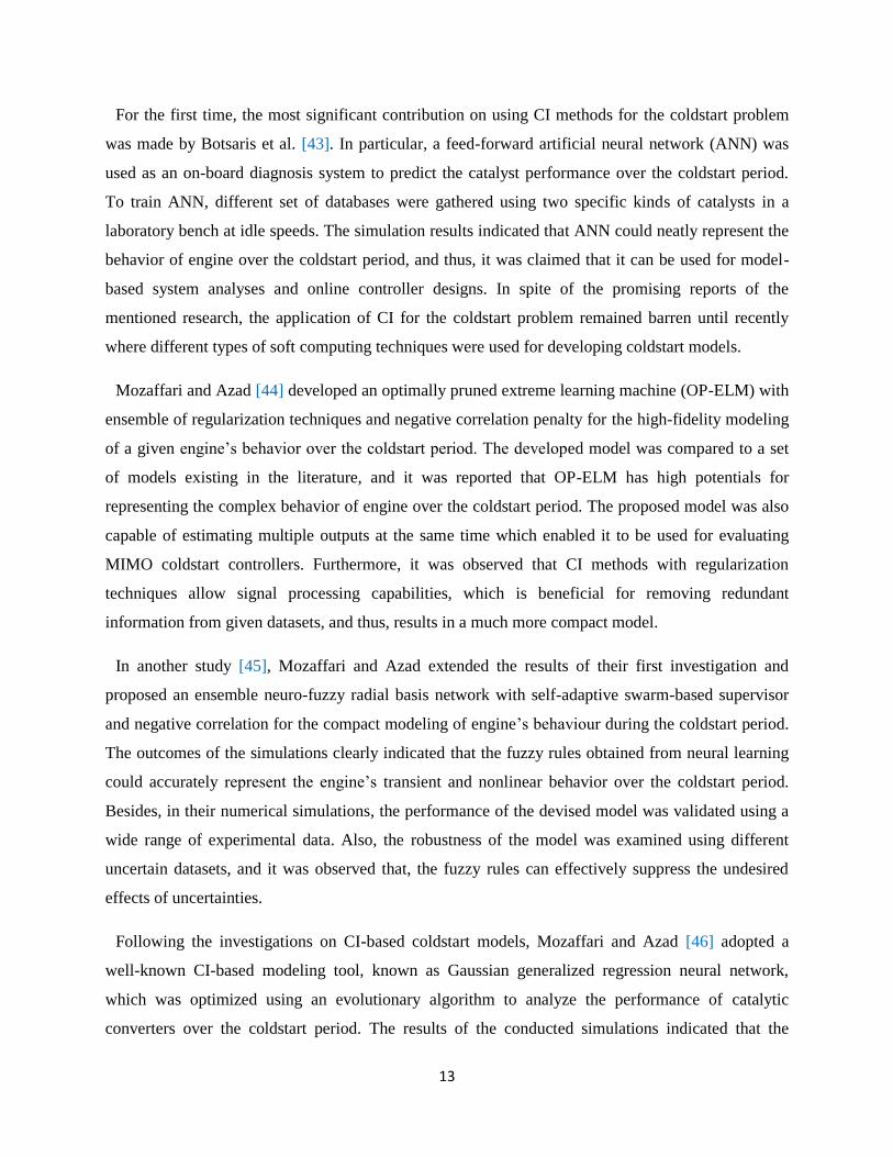
experimental bed belongs to the Vehicle Dynamics and Control Lab (VDL) at UCB. The

instrumented ICE engine is shown in Fig. 3-1. The test equipment used for measuring the

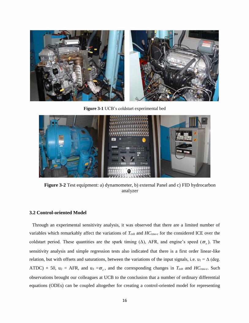
experimental signals is also depicted in Fig. 3-2

The engine has four cylinders with multi-port fuel injectors, along with an intake air control valve.

It has also the capability of producing up to 117 KW power at 5600 rpm. To simulate the engine

loads, the engine is coupled to a dynamometer. A dyno-controller is used to regulate the speed and

torque of the dynamometer. To measure the important signals of the considered ICE, for instance

air/fuel ratio (AFR), a number of sensors are taken into account. Also, an emission analyzer is

utilized for measuring the rate of HC emissions. The abovementioned setup is used to capture the

required information for developing a control-oriented model. In the next subsection, the formulation

of the control-oriented model is presented.

16

Figure 3-1 UCB’s coldstart experimental bed

Figure 3-2 Test equipment: a) dynamometer, b) external Panel and c) FID hydrocarbon

analyzer

3.2 Control-oriented Model

Through an experimental sensitivity analysis, it was observed that there are a limited number of

variables which remarkably affect the variations of Texh and HCraw-c for the considered ICE over the

coldstart period. These quantities are the spark timing (Δ), AFR, and engine’s speed ( e ). The

sensitivity analysis and simple regression tests also indicated that there is a first order linear-like

relation, but with offsets and saturations, between the variations of the input signals, i.e. u1 = Δ (deg.

ATDC) + 50, u2 = AFR, and u3 = e , and the corresponding changes in Texh and HCraw-c. Such

observations brought our colleagues at UCB to the conclusion that a number of ordinary differential

equations (ODEs) can be coupled altogether for creating a control-oriented model for representing

17

the engine’s coldstart behaviour. The formulated ODE representation of the coldstart state-space

model is given below [8]:

1 11 1

1 1

3 22 2

2 2

323 3

3 3

3 44 4

4 4

525 5

5 5

1 1 66 6

6 6

16

800

16

55 55

2

u kx x

u kx x

kux x

u kx x

kux x

u u kx x

(3-1)

The values of the internal parameters of the above control-oriented model are listed in Table 3-

1. It is worth mentioning that the second and fourth states are only functions of the engine speed

which is a known signal, and thus, are not considered for the implementation of the predictive

controllers.

Table 3-1 Internal parameter values for the control-oriented model

τ1 τ2 τ3 τ4 τ5 τ6

2.9629 156.2661 0.1800 1.1667 0.0002 0.0150

k1 k2 k3 k4 k5 k6

0.1997 5.2708 0.8527 0.1667 0.001 0.0075

From the above 6 state equations, the first three are used to find the values of Texh, and the last

three state equations are used to determine the values of HCraw-c. The standard formulation used

for the estimation of those output signals are, as follows:

1 3 2max ,0exhT t x t x t x t (3-2)

4 5 6max 4000 ,800 max ,0raw cHC t x t x t x t (3-3)

where, Texh and HCraw-c are in C and ppm, respectively.

18

To prepare the developed model to be used at the heart of predictive controllers, it is mandatory to

reformulate the above differential state-space model in a difference state-space form. Using the

Runge-Kutta method, the discrete-time form of the state-space model given in Eq. (3-1) can be given,

as follows:

1 11 1

1 1

3 22 2

2 2

2 33 3

3 3

3 44 4

4 4

2 55 5

5 5

1

6

11 1

11 1

16 11 1

1 8001 1

16 11 1

1 55

u k t kx k t x k

u k t kx k t x k

u k t kx k t x k

u k t kx k t x k

u k t kx k t x k

u kx k t

1 66

6 6

1 551 1

2

u k t kx k

(3-4)

To make sure that the control-oriented model works properly, a validation test for certain input

signals has been carried out. Figure 3-3 compares the experimental data versus the control-oriented

model predictions for Texh and HCraw-c. It is clear that the model has a good correlation with the

experimental data, which makes it a good fit to the coldstart control design.

The input signals should be confined within a logical range. To do so, the physical behavior of the

engine should be taken into account. One way to reduce the coldstart HC emissions is to increase Texh

as fast as possible to warm-up the catalytic converter, and thus, enhance its conversion efficiency.

Traditionally, this has been accomplished by the spark timing retard strategy. However, retarding the

spark timing can lead to reduced engine torques, which will cause a potential drivability issue.

Furthermore, exposing the catalytic converter to excessive Texh can generate more thermal stresses

and reduce its service life. Therefore, the spark timing retard should have a limit.

19

Figure 3-3 Validation of the model against experimental signals

Another method to reduce the coldstart HC emissions is to use a lean fuel strategy, which is

equivalent to a higher AFR. However, this may cause the combustion instability. Thus, to avoid this

problem, there should be a higher value for AFR, as well.

Based on the above-mentioned practical considerations, the first two inputs are confined within the

ranges below:

1

2

40 60

10 16

u

u

(3-5)

The input signal u3 is considered as a known external input. Given this fact, the engine system

states can be represented as x = [x1, x3, x5, x6] because, at every time step, the other variables x2 and x4

can be calculated beforehand using the values of signal u3.

As mentioned previously, the value of HCcum depends on the conversion efficiency of catalyst (η).

Based on experimental observations [19], the following equation has been proposed for η:

1 21 1 (3-6)

20

where:

1

2 0

1 1

max u ,0exp

m

kk a

(3-7)

2

0 0

2 2

max ,exp

m

cat cat cat

cat

T k T Tk a

T

(3-8)

The equation parameters, that is, a1, a2, m1, and m2, have been identified by experimental data. The

catalyst temperature (Tcat) primarily depends on Texh as the exhaust gas temperature is a major source

of the catalyst warm-up. These quantities are approximately proportional:

cat cat exhT k k T k (3-9)

Finally, the following equation can be used to determine the value of HCcum:

6

0 0

161 1 10

28.5

T T

raw exh ra cm wcuH dt HHC dm tC C

(3-10)

Based on experimental observations, the exhaust mass flow rate exhm is approximately proportional

to u3:

231 bubmexh (3-11)

The considered control-oriented model can be used at the heart of any discrete-time model-based

controller to calculate the coldstart controlling signals. Having said that the formulated objective

function for each predictive controlling strategy is specific. Thus, based on the above-mentioned

model, different types of objective functions are defined to design different versions of predictive

optimal controlling strategies for the coldstart problem in the next chapter.

21

Chapter 4

Coldstart Predictive Control Strategies

This chapter is devoted to the detailed descriptions of the proposed predictive control strategies,

namely nonlinear model predictive controller (NMPC), preference-based model predictive

controller (PBNMPC), and receding horizon sliding controller (RHSC), as well as presenting their

results for controlling the considered engine over the coldstart period. At the end of this chapter,

some important remarks can be inferred regarding the applicability of predictive control strategies for

the coldstart control problem.

4.1 Nonlinear Model Predictive Controller (NMPC)

The first considered controller is a standard model-based predictive optimal controller which is

suited for nonlinear controlling problems. The controller consists of two important parts. The first

part is the controlling module which works based on predicting the future behavior of plant. The

second part of NMPC is an optimization module which is suited for optimizing nonlinear objective

functions. The detailed formulation of the proposed controller is presented in the rest of this

subsection, and finally, the results of simulations together with a number of comparative numerical

tests are given to assess the potentials of the standard NMPC to deal with the coldstart problem.

4.1.1 Controller Formulation

Recently, nonlinear model predictive controllers have gained a remarkable attention from control

engineers due to their efficient performances [46, 47]. Such controllers are, in particular, effective for

a process in which a good model representing the plant behavior is available. The potential of NMPC

controllers for making decisions based on the prediction of future behavior of the system enables

them further enhance the quality of control commands, as compared to the other control techniques

[48]. A comprehensive literature review together with detailed descriptions of different NMPC

formulations can be found in [49]. For the sake of brevity, here, we avoid providing the details and

background information of NMPC design technique as it has extensively been done before. Rather,

22

the focus of this subsection will be on developing the mathematical formulation of NMPC controller

for the coldstart problem.

Let us consider the following state-space representation of the system:

1 , , ,k k k k f (4-1)

where shows the parameters of the model f, and χ and υ are the augmented state and input

matrices, as follows:

1

1

1

2

3

6

;

x ku k

x kk k u k

u kx k

(4-2)

Two sequential signals are captured after every t sec, which is calculated by PHt

N . As it

can be inferred, the time-difference depends on the prediction horizon and the number of set

points. The initial values of the states are also set as given below:

00 11.25 11.25 11.25 0 0 0

3

T

cat

cat

T

k

(4-3)

Let us now assume that Texh and HCraw-c are derived using the following equations:

1 2 3, , , ,exhexh TT k x k x k x k k q (4-4)

4 5 6, , , ,raw craw c HCHC k x k x k x k k

h (4-5)

The output vector of the plant, y, can be derived found by:

exh

raw c

T ky k

HC k

(4-6)

As mentioned previously, the input signals u1 and u2 are confined within a predefined range.

However, there are more constraints concerned with the variations of inputs (Δu) over the control

23

horizon (Hu) that should be considered. Here, these additional constraints are taken into account to

eliminate the input signal oscillations, as given below:

max min max min

1 1 1 1 1 1 1

max min max min

2 2 2 2 2 2 2

ˆ ˆ ˆ| 0.02 1| | 0.02

ˆ ˆ ˆ| 0.02 1| | 0.02

u k i k u u u k i k u k i k u u

u k i k u u u k i k u k i k u u

(4-7)

The augmented matrix derived from the equation above can be expressed by:

1

2

u kk

u k

(4-8)

The above-mentioned equations represent the states, outputs and inputs of the system only for one

set point. However, to proceed with the NMPC calculations, we need to define more general matrices

to include the present and future predicted values. Such an implementation is necessary for the

calculations of the NMPC controller’s objective function for pre-defined control and prediction

horizons. If the control and prediction horizons at each working point are indicated by HP and Hu,

respectively, these general matrices can be defined as:

ˆ ˆ| |

ˆ ˆ1| 1|;

ˆ ˆ1| 1|u u

k k k k

k k k kU U

k H k k H k

(4-9)

1| 1|

2 | 2 |;

| |P P

k k y k k

k k y k kX Y

k H k y k H k

(4-10)

The objective function at the heart of NMPC can be given as follows:

1

^6

1 2

1 0

16ˆ ˆ ˆ1 | | 10 | | |

28.5

uPHH

exh raw c

i i

J k k i k k i k HC k i k u k i k u k i km

(4-11)

where, HP represents the prediction horizon, Hu indicates the control horizon, and (k + i | k) shows

the prediction at time step k + i based on its value at time step k. The second term of the objective

function was added to the original formulation for HCcum to make sure that the control input signals

24

determined over the control horizon will be smooth and do not show illogical oscillations. The above

objective function, i.e. J (k), can be easily solved at each working point k.

By solving the objective function, the optimum profiles of the input signals, namely υ*, for the

upcoming horizon can be determined. The obtained profile is used by the controller to reduce the

value of HCcum. In most of the cases, the updating time of the controller tu is less than the time

required for the completion of HP. Let us investigate this concept mathematically:

/&

/

P

u

N H N tm N

m t m t

(4-12)

The above equation indicates that the optimizer used for the NMPC controller should be fast

enough to complete the calculations in a time period shorter than tu to guarantee the proper

performance of the controller. Obviously, the best control performance can be achieved if one can

reduce the updating time (tu) and increase the prediction horizon (that is, the value of N) as much as

possible, at the same time.

Figure 4-1 indicates a schematic illustration of the NMPC control operation for HCcum

reduction as well as the notion of prediction horizon, updating time, and control horizon.

Figure 4-1 Schematic illustration of NMPC

25

4.1.2 Online Optimizer

In the previous subsections, we indicated that for the NMPC controller implementation, the

considered optimizer should be powerful enough to converge to the optimum solution, and also, fast

enough to terminate the required calculations in a very short period of time. Recently, multi-agent

bio-inspired optimizers have successfully been applied for NMPC control applications and

demonstrated their capability for meeting the above-mentioned criteria [50, 51]. In the light of such

promising reports, here, we have been motivated to test the potential of an advanced bio-inspired

population-based optimizer (DPSO) for the coldstart control problem. In this subsection, a detailed

description of DPSO is provided.

DPSO combines the notions of social interactions among species with microbial life in the nature

[52]. Numerical investigations have demonstrated that DPSO is a good fit for optimization problems

in which the objective landscape dynamically varies over time. The initial algorithmic structure of

DPSO includes several random parameters and random samplings. This can increase the exploration

capability of DPSO for complex landscapes. However, as an online optimizer at the heart of NMPC

controller, some revisions should be exerted to its structure to make sure that a certain degree of

exploitation among its agents is guaranteed, which in turn results in the convergence of the

algorithm. To this aim, here, we modify the structure of DPSO slightly to boost the exploitation rate

among its agents. It is necessary to mention that the revisions are only exerted on the control

parameters of algorithm and the structure of DPSO remains unchanged. The main reason behind

increasing the exploitation (convergence speed) of DPSO lies in the fact that the online optimizer for

the NMPC controller should be capable of finding an acceptable optimum profile in a very short

period of time (less than tu) [49].

The original DPSO technique, known as dynamic hybrid PSO (DHPSO), has four main operators,

namely, the detection of dynamic changes, updating particles positions, reproduction and aging [52].

Based on our assessment, the last two operators can be removed from the structure of DHPSO as

they increase the computational complexity and foster the exploration of agents. As an NMPC solver,

DPSO which includes some mechanisms for the dynamic change detection and position updating,

can show a very fast convergence to an acceptable solution. Also, its algorithmic structure enables us

performing a mathematical analysis to make sure that the convergence can be guaranteed. The

important feature of DPSO/DHPSO is the ability of detecting the dynamical change. Therefore, this

26

phase remains unchanged. Let us consider each agent of DPSO as a particle. The algorithmic

structure of DPSO is given below:

Initialization: DPSO has three main parameters, namely Np,min , Np,max and Nsentry, which should be

specified beforehand. Firstly, Np,max particles are initialized randomly. Then, the initialized particles

are divided into two sub-populations. In this way, the first Np,min particles are sent to the first sub-

population and the remaining particles are sent to the second sub-population. The velocity of each

particle (V) is randomly generated as well.

Detection of dynamic changes: At the beginning of optimization, at each updating point of the

control procedure, a detection mechanism is carried out to find out whether the control objective

function experiences any change. In this context, a pre-defined number of sentry particles, Nsentry, are

distributed over the solution space randomly. At the beginning of each optimization stage, their

fitness values are evaluated. If the fitness value of at least one of these sentry particles changes, it can

be inferred that the objective function undergoes a dynamic change. This means that DPSO should

re-organize its exploration/exploitation capabilities to be reconciled to the new solution landscape.

Once a dynamic change is detected, the fitness of all Np,max particles are re-evaluated and the best

Np,min particles are put into the first sub-population. The remaining particles are re-initialized, and

then, sent to the second sub-population. This strategy is very efficient for dynamic environments. On

the one hand, the experiences from the previous exploration/exploitation over the solution space are

preserved. On the other hand, the re-initialized particles give DPSO a flexibility to search with a

wider vision over the solution landscape, and possibly, identify the fruitful regions within the

solution space.

It is worth pointing of that the sentry particles do not participate in the optimization and are just

used for detecting possible dynamic changes in the solution space. Hence, the convergence of DPSO

depends on the behavior of the other particles.

Updating particles position: To update the position of all particles, the local best position of particles

(lbest) and the global best solution are found by DPSO, gbest, and the average position of the

solutions in the second sub-population (ave) should be determined. For a D dimensional problem, the

position of particle i at iteration t can be defined as ,1 , ,2 ,..., ,t

i i i iZ z t z t z t D .

Let us show lbesti, gbest, ave, and the velocity vector as:

27

[ ( ,1), ( ,2),..., ( , )]t

i i i ilbest l t l t l t N (4-13)

[ ( ,1), ( ,2),..., ( , )]tgbest g t g t g t N (4-14)

,1 ,a ,2 ,...,a ,tabest a t t t D (4-15)

,1 , ,2 ,..., ,i i i iV t v t v t v t D (4-16)

Then, the updating rule of the particles can be implemented as below:

1t t t t t t

i i i i i iV V gbest Z ave Z lbest Z (4-17)

1 1t t t

i i iZ Z V (4-18)

where , , and are the inertia weight, social coefficient, and cognitive coefficient, respectively.

κ is a new parameter which verifies the impact of the re-initialized solutions in the second sub-

population on the searching characteristics of DPSO. As it can be inferred, the mentioned parameters

play a pivotal role on the movement of agents through the solution space.

Termination: After a pre-defined number of iterations (t), the optimization procedure is terminated

and the optimal profiles are used to control the coldstart operation of ICE.

The algorithmic structure of DPSO is presented in Figure 4-2.

4.1.3 Parameter Settings and Simulation Setup

There are a few parameters which should be set prior to proceeding with the simulations. The multi-

agent optimizer for the NMPC calculations possesses some controlling parameters which should be

verified. For spanning [0,0.7298] and within the range of [0, 1.7], it can be assured

that, eventually, DPSO converges to a stable point. At each stage of the calculations, DPSO

terminates the procedure once the difference between the objective values of two sequential iterations

becomes very small. DPSO performs the optimization with 20 particles from which the first half are

sent to the first sub-population and the remaining particles are sent to the second sub-population. To

ascertain the veracity of DPSO, two well-known optimization methods, golden search (GS) and

sequential quadratic programing (SQP) are taken into account.

28

Figure 4-2 Flowchart of the DPSO technique

For the GS algorithm, which is a sequential mini-max searching mechanism, the steps presented in

[53] are taken into account. If a change in the values of objective function between two sequential

iterations becomes very small, GS terminates its operation. SQP is also implemented based on the

steps described in [49]. The rival optimization techniques are implemented using Matlab. For SQP,

the existing Matlab solver is used, and the GS algorithm is encoded in a Matlab M-file. The stopping

criterion of GS is the number of iteration number and equals to 30, and the stopping criterion of SQP

is the convergence which is at the heart of Matlab’s SQP optimization tool.

For the classical optimal controller, the PMP algorithm is considered. The detailed descriptions of

the steps required for the implementation of PMP can be found in [8].

29

Figure 4-3 Considered engine speed profiles during the coldstart period (external inputs)

The engine speed profile (u3 = e ) is treated as a known external input and should be fed to the

devised NMPC controller during the coldstart period. For all of the simulations in this thesis, we

conduct the simulations for three different engine speed profiles, to check the performance of the

control system for different coldstart scenarios. The considered engine speed curves are depicted

in Figure 4-3.

All of the simulations are carried out using the Matlab software with Microsoft Windows 7

operating system on a PC with a Pentium IV, Intel core i7 CPU and 4 GBs RAM.

4.1.4 Simulation Results

In this subsection, two important objectives are pursued. Firstly, it is tried to conduct a comparative

study to investigate different features of the NMPC controller. This stage of the simulations includes

30

the evaluation of the efficacy of DPSO for the considered control problem, the robustness of DPSO,

and the performance of the NMPC controller compared to the rival classical optimal controller

designed based on PMP. At the second stage of simulations, the impact of prediction horizon (HP) on

the performance of the controller is investigated.

Based on a comparative study as well as our own assessment, for the first stage of the simulations,

the prediction horizon of 2 sec and the number of updating points of 15 are considered. The NMPC

controller re-calculates the input signals after every 0.26 sec. Table 4-1 lists the total HCcum resulting

from the NMPC computations with the DPSO, SQP and GS online optimizers as well as the required

time for the calculation of control commands at each stage of the process. It is worth noting that the

reported calculation time is the average of all calculations that an optimizer performs over the entire

control process. In this way, we will make sure that the reported time is a proper indicator of the

computational efficiency of each method. For all of the three cases, it can be seen that the

computational complexity of DPSO and GS are relatively the same and the both are more time-

consuming than SQP. Also, the results indicate that DPSO can yield better optimum solution

compared to GS and SQP. The other interesting observation relates to the better performance of SQP

in comparison with GS although it has less calculation time. This, in turn, implies that SQP is a better

online optimizer compared to heuristic methods; however, it cannot outperform DPSO. This is

mainly due to the efficient exploration/exploitation capability of the agents of DPSO. Given the fact

that the differences between the calculation time of SQP and DPSO never exceeds 0.04 sec, it can be

inferred that DPSO is a suitable online optimizer to be used at the heart of NMPC controller. As

mentioned before, DPSO is a multi-agent optimizer which uses stochastic operators, in the form of

random walks, to search the solution domain. This means that the solution suggested by DPSO may

not be the same over independent runs. If the variations of the obtained results over independent runs

become too large, the performance of NMPC controller can be degraded significantly. Therefore, a

numerical experiment is carried out to check the robustness of DPSO. Obviously, the higher

robustness of DPSO provides the better control performance. For checking the robustness of DPSO,

there is no choice but to repeat the optimization for a number of independent runs and calculate the

variation of the obtained solutions in terms of the standard variation (std.). Here, the optimization

procedure is repeated for 10 independent runs for each of the three cases. Table 4-2 presents the

details of the obtained results in terms of the calculation time and total HCcum. Also, the statistical

results representing the main aspects of the NMPC computations for independent runs are reported in

Table 4-3.

31

Table 4-1 Comparison between the NMPC control performances with different online optimizers

Algorithms Case 1 Case 2 Case 3

Calculation time HCcum Calculation time HCcum Calculation time HCcum

SQP 0.039679 0.2321 0.038322 0.2335 0.036345 0.2353

GS 0.049294 0.2443 0.053316 0.2485 0.065345 0.2495

DPSO 0.060549 0.2105 0.061424 0.2187 0.073467 0.2251

Table 4-2 Performance of the NMPC controller over 10 independent runs

# Run Case 1 Case 2 Case 3

Calculation time HCcum Calculation time HCcum Calculation time HCcum

1 0.060549 0.2105 0.061424 0.2187 0.073467 0.2251

2 0.061322 0.2104 0.061812 0.2165 0.076564 0.2256

3 0.060835 0.2079 0.061333 0.2280 0.072929 0.2274

4 0.061500 0.2207 0.061463 0.2144 0.077763 0.2173

5 0.061337 0.2094 0.062092 0.2187 0.070773 0.2172

6 0.060856 0.2152 0.064675 0.2131 0.076469 0.2102

7 0.061416 0.2156 0.061416 0.2265 0.072382 0.2296

8 0.060329 0.2094 0.061337 0.2224 0.074392 0.2126

9 0.061416 0.2199 0.061322 0.2168 0.077670 0.2358

10 0.062150 0.2203 0.061506 0.2147 0.075762 0.2190

Table 4-3 Statistical results of the NMPC computations for independent runs

# Run Case 1 Case 2 Case 3

Calculation time HCcum Calculation time HCcum Calculation time HCcum

Best 0.0608 0.2079 0.0646 0.2131 0.0729 0.2102

Worst 0.0614 0.2207 0.0613 0.2280 0.0777 0.2358

Mean 0.0612 0.2139 0.0618 0.2190 0.0748 0.2220

Std. 5.3e-4 0.0050 0.0010 0.0051 0.0024 0.0080

By taking a peek at the obtained results, it can be seen that the NMPC calculation results over the

independent runs are very close to each other. This issue can be even further verified by considering

the low std. values. As it can be seen, the differences of the best, worst, and mean values of the total

emitted HCcum are negligible. The results augur the high robustness of the utilized online optimizer at

the heart of NMPC controller. This further endorses on the applicability of DPSO for NMPC control

applications.

After ensuring the acceptable performance of the controller with online DPSO optimizer, we intend

to compare its performance with an optimal control strategy designed based on PMP. This is

basically an offline controller which uses the same control-oriented model (but in its differential

equation form) to determine the optimal input profiles. PMP can afford the global optimum profiles;

however, that is difficult to implement it as an online control algorithm because the calculation of the

32

optimal solution over the coldstart period takes a few minutes. In the previous work by our research

group, it has been mentioned that the use of steepest descent method for PMP will slow down the

optimization process, and thus, hinders its applicability for online control applications [8]. However,

to deal with the plant model uncertainties and unknown disturbances, it is necessary to implement

real-time controllers for automotive coldstart applications. The proposed NMPC controller uses fresh

information about the engine system and performs an online optimization based on this information

(see Figure 4-1). However, when the pre-defined optimum inputs calculated offline by the PMP

algorithm are applied to the real engine, the control performance may be degraded significantly, due

to mismatches between the control-oriented model and the engine system. It is now important to find

out how much the near-optimal, but real-time, solutions suggested by the NMPC calculations are

different from those obtained by PMP. To be more precise, it is critical to make sure that the online

optimization performed by the NMPC controller does not reduce the quality of the optimum profiles.

Table 4-4 compares the results obtained by the PMP and NMPC control techniques. As it can be

seen, the difference between the mean performance of online NMPC and that of offline PMP controls

are not significant. This means that the NMPC technique can be reliably used to develop a real-time

controller for reducing HCcum over the coldstart period.

Prior to starting the second stage of numerical experiments, we would like to investigate the

physical behavior of the engine system by providing the obtained profiles.

Figure 4-4 indicates the optimum AFR profiles obtained by the NMPC controller. It can be inferred

that, to minimize HCcum, the proportion of air/fuel mixture should always remain lean (AFR ≈ 15-16).

Figure 4-5 depicts the optimum profiles of spark timing. As it can be seen, for all of the three cases,

the NMPC controller leads the value of Δ from 5 deg. BTDC to 10 deg. ATDC within the first 10

seconds and retains the profile at the relatively same degree for the remaining 40 seconds. As it was

indicated in Table 4-4, when the engine speed is at the highest level, the minimum of HCcum is the

lowest. This is mainly due to the fact that by increasing the engine speed, the debit of exhm is

increased. Figure 4-6 depicts the profile of Texh for the three cases. It can be seen that by increasing

the engine speed, the exhaust gas temperature increases. This means that more heat is provided to

increase the catalyst temperature which in turn incurs a faster catalyst warm-up. According to Figure

4-7, such a behavior results in an increase in the value of catalyst conversion efficiency. Figure 4-8

indicates the real-time raw HC emission rate. For all of the three cases, there is a peak in the engine-

out HC emission rate. The experiments have shown that this initial peak is necessary for reducing the

33

risk of engine stalling. It can be also inferred that by increasing the engine speed, the rate of engine-

out HC emissions reduces to lower levels in a shorter period of time.

Table 4-4 Results obtained by the online NMPC and offline PMP controllers

Controller Case 1 Case 2 Case 3

PMP 0.145 0.158 0.218

NMPC 0.213 0.219 0.222

Figure 4-4 Optimum AFR profiles obtained by NMPC

34

Figure 4-5 Optimum Δ profiles obtained by NMPC

Figure 4-6 Optimum Texh profiles obtained by NMPC

35

Figure 4-7 Catalyst efficiency for the optimum solutions

Figure 4-8 Engine-out HC emissions rate for the optimum solutions

36

In the second stage of the numerical experiments, the impact of prediction horizon length on the

performance of controller is evaluated. For this sake, the control action calculation procedure is

repeated for 6 different prediction horizons, that is, 1, 2, 3, 4, 5, and 6 sec. It is worth pointing out

that the number of set points for each stage of the calculations is adjusted so that the values of

updating time (tu) and t remain constant. Table 4-5 presents the results of the simulations. As it can

be seen, by increasing the length of HP, the value of HCcum is reduced. However, this results in an

increase in the calculation time. It is interesting that for HP of 6 sec, the total emitted HC is relatively

the same as that for PMP. However, as it can be seen, the calculation time exceeds the updating time,

and thus, the results are not suitable for practical applications. Therefore, for implementing the

proposed NMPC coldstart controller in real-time, we have no choice but to accept the near-optimal

solutions at the expense of lower computational costs.

The results of simulations indicated that the NMPC technique can outperform the PMP algorithm in

terms of the computational efficiency for the coldstart problem. Also, through a theoretical analysis,

it was demonstrated that the proposed multi-agent optimization DPSO technique can guarantee the

convergence of the NMPC calculations within a finite number of iterations. Moreover, the

comparative results indicated that the proposed multi-agent optimizer can outperform golden search

(GS) and sequential quadratic programming (SQP) for calculating the control commands. The

numerical experiments also indicated that by increasing the prediction horizon as well as the number

of updating points, the results of the NMPC calculations can be improved. However, it was observed

that to achieve such better results in terms of the performance optimality, a higher computational

budget is required, and thus, there is a trade-off between the optimality and online implementation

potential of the NMPC controller.

Table 4-5 Performance of the NMPC controller with different prediction horizons

HP (sec) Case 1 Case 2 Case 3

Calculation time HCcum Calculation time HCcum Calculation time HCcum

1 0.0586 0.2185 0.0579 0.2205 0.0674 0.2313

2 0.0612 0.2139 0.0618 0.2190 0.0748 0.2220

3 0.0675 0.1847 0.0683 0.1912 0.0894 0.2214

4 0.0854 0.1845 0.0912 0.1886 0.0988 0.2205

5 0.1442 0.1772 0.1231 0.1824 0.1425 0.2201

6 0.1546 0.1453 0.1423 0.1653 0.1562 0.2186

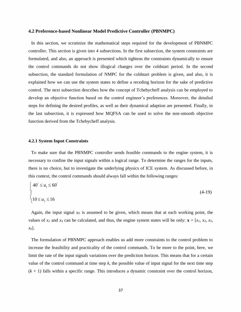
37

4.2 Preference-based Nonlinear Model Predictive Controller (PBNMPC)

In this section, we scrutinize the mathematical steps required for the development of PBNMPC

controller. This section is given into 4 subsections. In the first subsection, the system constraints are

formulated, and also, an approach is presented which tightens the constraints dynamically to ensure

the control commands do not show illogical changes over the coldstart period. In the second

subsection, the standard formulation of NMPC for the coldstart problem is given, and also, it is

explained how we can use the system states to define a receding horizon for the sake of predictive

control. The next subsection describes how the concept of Tchebycheff analysis can be employed to

develop an objective function based on the control engineer’s preferences. Moreover, the detailed

steps for defining the desired profiles, as well as their dynamical adaption are presented. Finally, in

the last subsection, it is expressed how MQFSA can be used to solve the non-smooth objective

function derived from the Tchebycheff analysis.

4.2.1 System Input Constraints

To make sure that the PBNMPC controller sends feasible commands to the engine system, it is

necessary to confine the input signals within a logical range. To determine the ranges for the inputs,

there is no choice, but to investigate the underlying physics of ICE system. As discussed before, in

this context, the control commands should always fall within the following ranges:

1

2

40 60

10 16

u

u

(4-19)

Again, the input signal u3 is assumed to be given, which means that at each working point, the

values of x2 and x4 can be calculated, and thus, the engine system states will be only: x = [x1, x3, x5,

x6].

The formulation of PBNMPC approach enables us add more constraints to the control problem to

increase the feasibility and practicality of the control commands. To be more to the point, here, we

limit the rate of the input signals variations over the prediction horizon. This means that for a certain

value of the control command at time step k, the possible value of input signal for the next time step

(k + 1) falls within a specific range. This introduces a dynamic constraint over the control horizon,

38

which can be taken into account properly by MPC controllers. The mathematical formulations of

these constraints are given below:

1 1 1 1 1

2 2 2 2 2

ˆ ˆ ˆ ˆ ˆ1| | | 1| |

ˆ ˆ ˆ ˆ ˆ1| | | 1| |

u k i k u k i k u k i k u k i k u k i k

u k i k u k i k u k i k u k i k u k i k

(4-20)

where, (k + i | k) shows the prediction at time step k + i based on its value at time step k, and Δu

represents the possible variation range of the input signal from a certain time step k + i - 1 to the next

time step k + i. The possible variation range of the input signals is calculated by:

max min max min

1 1 1 1 1 1 1

max min max min

2 2 2 2 2 2 2

ˆ ˆ ˆ1| 0.02 | 1| 0.02

ˆ ˆ ˆ1| 0.02 | 1| 0.02

u k i k u u u k i k u k i k u u

u k i k u u u k i k u k i k u u

(4-21)

4.2.2 Controller Formulation

By significant advancements of computational tools and processors, optimal predictive controllers

have been attracting remarkable attention from control engineers. The applicability of such

controllers has been started, first, by using them for controlling chemical processes. Later, such types

of controllers have been successfully applied to much more intricate process control tasks. The

research literature has clearly demonstrated the potential of optimal predictive controllers for the

calculations of control commands based on a system’s future behavior, which turns this type of

controller into one of the most promising control systems, compared to the other types of controllers

[47, 54]. In this subsection, the mathematical formulation of the considered control strategy is

described, and also, it is explained how it can be used for HCcum emission reduction during the

coldstart period. It is worth mentioning that the formulation below establishes the most critical part

of PBNMPC controller. The state-space representation of the engine system given in the previous

chapter can be shown in the following nonlinear algebraic form:

1 , , ,k k k k X f X U (4-22)

39

where, is the matrix of the internal parameters of the system, f represents a set of discrete

nonlinear equations, and also, X and U are the augmented forms of the state and the input matrices,

respectively, given below:

1

1

1

2

3

6

;

x ku k

x kk k u k

u kx k

X U (4-23)

Similar to the previous controller design, the initial values of the states are:

0 11.25 11.25 11.25 0 0 0T

X (4-24)

As a discrete system, the time interval of the state-space representation should be verified. The

NMPC controller uses two key parameters to calculate the control commands at each updating point.

These parameters are the prediction horizon (HP) and the number of set points (N) considered for

discretizing HP. Based on the above-mentioned concepts, the time interval t is given by:

PHt

N (4-25)

It is worth noting that the values of the above parameters can be adjusted to make sure that the

predictive controller works properly to achieve high-performances in real-time applications. At each

set point, the engine system outputs Texh and HCraw-c can be calculated, and thus, the augmented

output matrix is given by:

exh

raw c

T kk

HC k

Y (4-26)

Another matrix which should be defined is the augmented form of the input signals variations:

1

2

u kk

u k

U (4-27)

Now, the key point is the way of assembling the above parameters and information to construct

the predictive controller for our case study. This can be done by applying the concept of receding

40

horizon as well as the creation of a proper objective function (J). Thus, the first step is to define

more general matrices to concatenate the present and future values of the above augmented

matrices. Let us consider that at each updating point of the controller calculations, the

computations should be performed for a pre-defined control horizon (HU) and prediction horizon

(HP).

The general form of the receding horizon-based matrices for U and ΔU are given by:

* *

ˆ ˆ| |

ˆ ˆ1| 1|ˆ ˆ;

ˆ ˆ1| 1|U U

k k k k

k k k k

k H k k H k

U U

U UU U

U U

(4-28)

Also, the general form of the receding horizon-based matrices for X and Y are expressed by:

* *

| |

ˆ ˆ1| 1|;

ˆ ˆ| |P P

k k k k

k k k k

k H k k H k

X Y

X YX Y

X Y

(4-29)

Using the above information, a proper objective function J will be defined for the NMPC

controller, as follows:

1

2 2* *

( ) R( )1 0

ˆ ˆ| | |uP

HH

dQ i i

i i

k i k k i k k i k

J Y Y U (4-30)

By optimizing the above objective function, the optimum values of control commands U* for the

upcoming horizon will be determined. Obviously, the optimization algorithm should be fast enough

to calculate the proper commands in a very short period of time.

In many of the existing optimal coldstart controllers, such as NMPC, equation below has been used

as the objective function J:

2 1

^ 26 *

R( )1 0( )

16 ˆˆ1 | | 10 | |28.5

uPHH

exh raw ci

i iQ i

k i k k i k HC k i k k i km

J U (4-31)

41

As it can be seen, the above objective function depends on several quantities, including the

conversion efficiency which increases the complexity of computations. This is a critical issue when

using the controlling technique in real-time as the required calculations should be done in a very

short period of time. To overcome such an important problem, in the formulation of PBNMPC, a

modified objective function with less complexity will be employed to calculate the control

commands much faster. Moreover, instead of using sequential quadratic programming (SQP), a very

fast and robust optimization algorithm will be applied which is best suited for solving the non-

smooth, non-convex optimization problem within the PBNMPC formulation. Through simulations, it

will be indicated that the proposed objective function is very efficient for the coldstart HCcum

reductions.

4.2.3 Tchebycheff preference for desired trade-offs

As mentioned previously, there is a dilemma on how to change the input signals during the coldstart

to minimize HCcum because there is a trade-off between the variations of Texh and HCraw-c in response

to the inputs [55]. From a mathematical perspective, the Pareto theory states that the confliction

between two arbitrary quantities f1 and f2 can result in a non-dominated front known as the Pareto

front. The optimal Pareto front refers to a curve which includes a number of solutions resulting from

the optimal trade-offs between f1 and f2. To be more to the point, this theory expresses that in such a

condition, it is impossible to come up with a unique optimum solution and there exist a lot of

optimum pairs of f1 and f2 which can be considered as the optimized solution to a conflicting

objective function J. Hence, formulating a simpler objective function for the coldstart problem purely

based on Texh and HCraw-c can lead the NMPC controller (or any other optimal controller) towards

various input profiles. One remedy to this challenging confliction is to define weights for the both

Texh and HCraw-c to direct the control strategy towards certain profiles, as given below:

1 1 2 2min : f f J (4-32)

Considering two conflicting quantities with the above form helps the optimizers always seek for a

particular trade-off. However, there is no guarantee that the final solution converges to the optimum

Pareto front. To be more precise, for a certain trade-off, there is also a possibility that the quality of

the final solution can be further improved. The Tchebycheff approach is a mean for converting the

problem of approximating a Pareto front into a number of preference-based scalar optimization

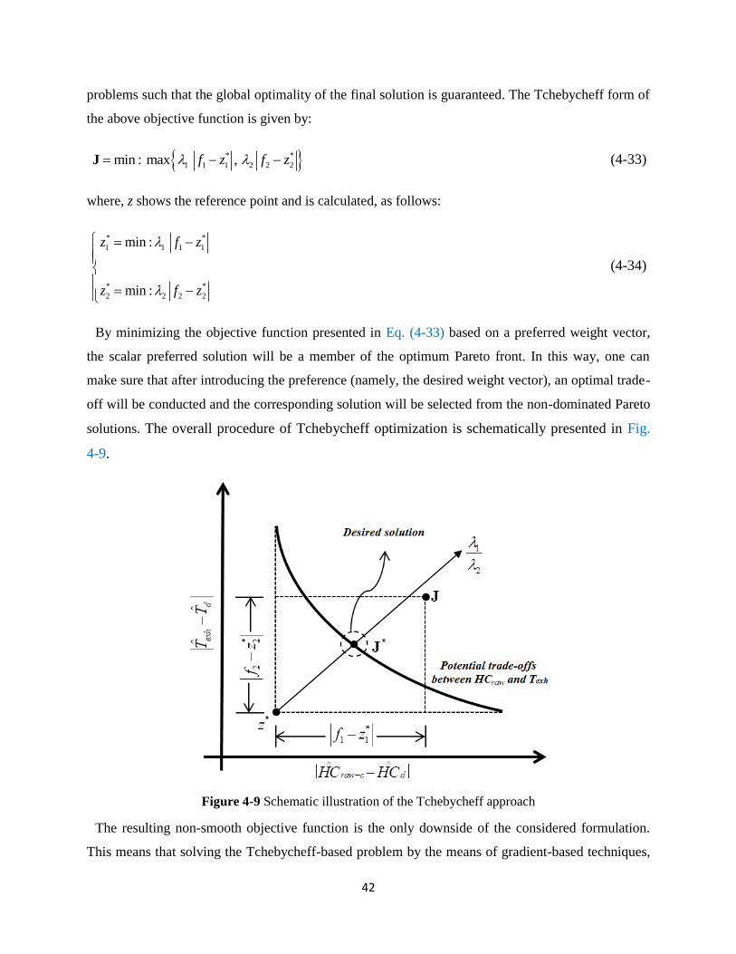
42

problems such that the global optimality of the final solution is guaranteed. The Tchebycheff form of

the above objective function is given by:

* *

1 1 1 2 2 2min : max ,f z f z J (4-33)

where, z shows the reference point and is calculated, as follows:

* *

1 1 1 1

* *

2 2 2 2

min :

min :

z f z

z f z

(4-34)

By minimizing the objective function presented in Eq. (4-33) based on a preferred weight vector,

the scalar preferred solution will be a member of the optimum Pareto front. In this way, one can

make sure that after introducing the preference (namely, the desired weight vector), an optimal trade-

off will be conducted and the corresponding solution will be selected from the non-dominated Pareto

solutions. The overall procedure of Tchebycheff optimization is schematically presented in Fig.

4-9.

Figure 4-9 Schematic illustration of the Tchebycheff approach

The resulting non-smooth objective function is the only downside of the considered formulation.

This means that solving the Tchebycheff-based problem by the means of gradient-based techniques,

43

for instance the steepest descent algorithm, may not provide the correct solution. However, we apply

the above technique to the coldstart problem to form the objective function of PBNMPC controller.

Let us write the objective function of coldstart problem as given below:

2

^ ^ 2

1 2

1

ˆ ˆmin : max | | , | |PH

raw c d exh d

i

HC k i k HC k i k T k i k T k i k

J (4-35)

It can be seen that the both terms are formulated as minimization problems. This is because, the two

terms present the distances of the values of HCraw-c and Texh from the desired profiles (HCd and Td),

instead of the minimization of HCraw-c and the maximization of Texh. By defining certain values of the

weights, the above scalar objective function can converge to a preferred non-dominated solution.

However, there is one critical issue which should be verified. It is important to find out which pair of

the weights can afford an optimal solution which is best compatible with the underlying physics of

the problem. In fact, it should be verified that the control commands should be in favor of decreasing

HCraw-c or increasing Texh. To find out the characteristic of the desired solution, a primary test is

conducted. In this way, the single version of the objective function with three sets of the weights is

considered and an offline control algorithm is used to investigate the impact of each scenario on the

quality of the final solution. The single version of the objective function and the three pairs of the

weights are given below:

2

^ ^ 2

1 2

1

ˆ ˆmin : | | | |PH

raw c d exh d

i

HC k i k HC k i k T k i k T k i k

J (4-36)

11

2

12

2

13

2

: 0.80

: 1.00

: 1.25

C

C

C

(4-37)

For the offline calculations, the desired profiles of the system outputs are calculated based on the

following values of input signals [56]:

1 2

1 2

: 5deg ; 15.9

: 10deg ; 14.9

d

d

HC u ATDC u

T u ATDC u

(4-38)

44

The results of the sensitivity analysis indicate that by increasing the value of α from 0.8 to 1.25, the

minimum of HCraw-c will be decreased (0.2423 g, 0.2357 g and 0.2257 g, respectively). This

demonstrates the further importance of minimizing HCraw-c, compared to the other term.

Based on the above analysis, the following objective function is considered for the PBNMPC

controller:

2

^ ^ 2

1

ˆ ˆmin : max 1.25 | | , | |PH

raw c d exh d

i

HC k i k HC k i k T k i k T k i k

J (4-39)

One of the remarkable advantages of the proposed PBNMPC scheme over other control algorithms

lies in its capability to revise the desired profile in a real-time fashion based on the status of the

system. In the offline calculations of the desired profiles, Eq. (4-38) is taken into account. However,

these off-line calculations are performed regardless of the simplifications/assumptions used for the

development of the coldstart model. Assume that under specific conditions, the engine system is

inflicted in reality by some unknown and unpredictable disturbances or parameter variations.

Therefore, the controller which is using the predefined desired trajectories provides improper

commands, resulting in a poor performance with high HCcum. If we can devise a policy to update the

calculation of the desired profiles during the control process, it will enhance the performance of the

controller in such conditions when there is a mismatch between the coldstart model and the real

engine system behavior. The mentioned concept can be integrated with the PBNMPC strategy. In this

context, at each updating point, the states of the first set point (k = 1) of the prediction horizon are

replaced with the desired values of the states, and based on that, the prediction of the desired profile

for the remaining set points (k = 2 to N) are performed using the input values reported in Eq. (4-38).

Let us provide a mathematical definition for such a real-time desired profile builder. Suppose that the

PBNMPC controller is at the beginning of one of its updating points and should predict the actual

(Eq. (3-4)) and desired future states of the engine system. For the offline desired profile calculations,

it only needs to put the values reported in Eq. (4-38) in Eq. (3-4). However, in the online optimum

trajectory building scenario, the initial values (first set point) of the desired states are exactly the

same as those used for the prediction of actual profile with using the feedback of the engine states.

For the remaining set-points, the desired state values are predicted using the input signal variables

given in Eq. (4-38). This can be mathematically expressed as given below:

45

1 11 1

1 1

11 1

1 1

2 33 3

3 3

33 3

3 3

11 1 ; 2

601 1 ; 3,...,

16 11 1 ; 2

16 14.91 1 ; 3,...,

d

d d

d

d d

u k t kx k t x k k

t kx k t x k k N

u k t kx k t x k k

t kx k t x k k N

(4-40)

1 3 2max ,0d d

dT k x k x k x k (4-41)

2 55 5

5 5

55 5

5 5

1 1 66 6

6 6

66 6

6

16 11 1 ; 2

16 15.91 1 ; 3,...,

1 55 1 551 1 ; 2

2

1 1 ; 3,...,

d

d d

d

d d

u k t kx k t x k k

t kx k t x k k N

u k u k t kx k t x k k

t kx k x k k N

(4-42)

4 5 6max 4000 ,800 max ,0d d

dHC k x k x k x k (4-43)

It should be noted that the states x2 and x4 depend on u3 which is considered as a known input. Such

real-time updating of the desired profiles are advantageous for the coldstart controller in practice

where it is essential to track logical desired profiles to ensure proper HCcum reductions.

In the next subsection, we scrutinize the algorithmic structure of MQFSA to explain how the non-

smooth, non-convex objective function derived from the Tchebycheff analysis can be solved.

4.2.4 Multivariate quadratic fit-sectioning algorithm

To calculate the solution of objective function, here, a powerful non-derivative deterministic

optimization algorithm is introduced which can be considered as a multi-dimensional version of the

Brent’s method [57]. MQFSA comprises of two different operators, namely the quadratic fitting and

46

golden sectioning mechanisms. MQFSA performs the optimization for each dimension

independently, in a cooperative fashion. Firstly, we explain how the algorithm works (for one

dimension), and then, extend the mechanism to fit the operators for multivariate problems.

Quadratic fitting mechanism: At the beginning of the procedure, a three-step pattern including points

h1, h2, and h3 is formed which satisfies the following criterion:

2 1 3 1 2 3,h h h h h h J J J (4-44)

Thereafter, a quadratic polynomial is used to fit three points, which results in the following system

of equations:

2

1 1 1

2

2 2 2

2

3 3 3

h a bh ch

h a bh ch

h a bh ch

J

J

J

(4-45)

Solving the equation below helps us to calculate the value of c:

1 2 3 2

3 1 2 1 3 2

1 h h h hc

h h h h h h

J J J J (4-46)

Also, the minimum of J can be calculated by:

2 0t tQ b cQ J

(4-47)

2 31 2 12 2

t

h hh hQ

(4-48)

where:

2 1 3 2

2 1 3 2 3 2 1 2

h h h h

h h h h h h h h

J J

J J J J (4-49)

We use the following operator to update the patterns:

47

3 2 3

1 1 2

,

,

t t

t t

h Q if Q h h

h Q if Q h h

(4-50)

Let us consider that the optimum value at the current iteration is indicated by Qt. At the next

iteration, the optimum solution is known as Qt + 1. The current solution can be accepted if:

1 2 10.5t tQ Q h h (4-51)

Otherwise, the new solution Qt + 1 is rejected and the golden sectioning algorithm is used to

calculate Qt + 1.

Golden sectioning mechanism: This is a deterministic direct search strategy which uses a pre-

defined bound (h1, h3) for the optimization. Here, two solutions are determined using the

following formulation [57]:

3 13

3 11

1.6181

1.6181

h ha h

h hb h

(4-52)

Then, based on that, Qt + 1 is determined and the bounds are updated:

3

1 3

1

1 1

t

t

h aif a b

Q h

h bif b a

Q h

J J

J J

(4-53)

Thereafter, the termination criterion (maximum iteration) is checked, and if it is not satisfied, the

algorithm uses the criterion stated in Eq. (4-51) to select the proper operator. After termination of the

criterion, the optimization through the first dimension is completed. This optimum value is stored at

the vector of the solution and the same approach is used for the next dimension. Such a chain like

mechanism is continued until all of the dimensions are exposed to MQFSA. The flowchart of

MQFSA is given in Fig. 4-10. Based on the above definitions, the detailed block diagram of

PBNMPC controller is presented in Fig. 4-11.

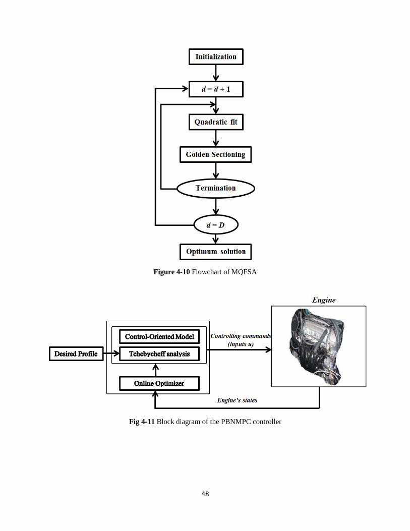
48

Figure 4-10 Flowchart of MQFSA

Fig 4-11 Block diagram of the PBNMPC controller

49

4.2.5 Parameter Settings and Simulation Setup

To conduct the simulations, the controller and some pre-defined profiles should be introduced. The

controller consists of an optimizer and a control-oriented model. The detailed descriptions of the

model and MQFSA were given previously. Other than MQFSA, the golden search (GS) algorithm is

taken into account to check the efficacy of the proposed method for the PBNMPC calculations.

Moreover, we use the standard nonlinear model predictive controller (NMPC) to further clarify the

advantages of the proposed controller. The NMPC problem is optimized by sequential quadratic

programming (SQP). It is worth noting that the both MQFSA and GS algorithms conduct the

optimization within the range of unity, and also, the mapping to the real solution space is performed

in the objective function. Based on this point, the extremes of each domain are taken as a = 0 and b =

1. To compare the performance of the proposed controller with a classical optimal controller, the

Pontryagin’s minimum principle (PMP) is considered. In our simulations, the engine speed profile

(u3 = e ) is a given external input and this is provided to the controller in the coldstart period. It is

worth noting that for the development of NMPC and PBNMPC controllers, the prediction horizon

length (HP) of 2 sec is taken into account, and at each updating point, the horizon interval is divided

into 15 set-points (N = 15).

The simulations are conducted under the three conditions used for the previous simulations. The

computational facilities and encoding environments are exactly the same as those of the previous

simulation.

4.2.6 Simulation Results

The simulation results can be categorized into four different parts. In the first part, we conduct a

comparative study to demonstrate the efficiency of MQFSA for the optimization of the non-smooth

objective function derived from Tchebycheff analysis. Thereafter, the effectiveness of PBNMPC

approach is evaluated by repeating the simulations for 10 independent runs. At the third stage,

statistical tests are provided to study the advantages of PBNMPC over the standard NMPC strategy

with the conventional objective function. Finally, the performance of online PBNMPC controller is

compared with the offline optimal controller derived from PMP.

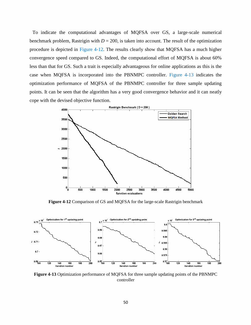
50

To indicate the computational advantages of MQFSA over GS, a large-scale numerical

benchmark problem, Rastrigin with D = 200, is taken into account. The result of the optimization

procedure is depicted in Figure 4-12. The results clearly show that MQFSA has a much higher

convergence speed compared to GS. Indeed, the computational effort of MQFSA is about 60%

less than that for GS. Such a trait is especially advantageous for online applications as this is the

case when MQFSA is incorporated into the PBNMPC controller. Figure 4-13 indicates the

optimization performance of MQFSA of the PBNMPC controller for three sample updating

points. It can be seen that the algorithm has a very good convergence behavior and it can neatly

cope with the devised objective function.

Figure 4-12 Comparison of GS and MQFSA for the large-scale Rastrigin benchmark

Figure 4-13 Optimization performance of MQFSA for three sample updating points of the PBNMPC

controller

51

Table 4-6 Comparison between the performances of PBNMPC controllers with different online

optimizers

Algorithms Case 1 Case 2 Case 3

Calculation time HCcum Calculation time HCcum Calculation time HCcum

GS 0.043928 0.1623 0.044226 0.1753 0.048857 0.1773

MQFSA 0.046078 0.1530 0.046078 0.1574 0.051285 0.1623

Table 4-7 Performance of the PBNMPC controller over 10 independent runs

# Run Case 1 Case 2 Case 3

Calculation time HCcum Calculation time HCcum Calculation time HCcum

1 0.046051 0.1525 0.046423 0.1577 0.051329 0.2241

2 0.046214 0.1536 0.046321 0.1573 0.051121 0.2254

3 0.046153 0.1533 0.046312 0.1574 0.051183 0.2125

4 0.046003 0.1523 0.046421 0.1571 0.051335 0.2142

5 0.046044 0.1537 0.046512 0.1574 0.051317 0.2111

6 0.046083 0.1535 0.046673 0.1573 0.051352 0.2143

7 0.046102 0.1521 0.046317 0.1577 0.051245 0.2310

8 0.046032 0.1522 0.046315 0.1575 0.051311 0.2112

9 0.046076 0.1528 0.046749 0.1570 0.051346 0.2142

10 0.046024 0.1537 0.046361 0.1577 0.051317 0.2155

Table 4-6 lists the results obtained by the PBNMPC controller with GS and MQFSA optimization

algorithms. The results are presented in terms of the calculation time and HCcum. It can be seen that

the PBNMPC strategy with MQFSA can further reduce HCcum in comparison with the PBNMPC

scheme with GS optimizer. The other important observation pertains to the relatively similar

computational time of the both optimizers, which, in turn, implies that MQFSA can efficiently be

reconciled to the computational requirements of the PBNMPC controller. From a physical point of

view, the performance evaluations of all controllers reveal that by imposing a higher engine speed,

the value of HCcum is decreased. Table 4-7 presents the results obtained by the PBNMPC controller

over 10 independent runs. By taking a precise look at Table 4-7, it can be easily inferred that the

obtained results are very similar. This, in turn, implies that the proposed PBNMPC approach is high-

performance and has the capability of real-time implementations.

Figure 4-14 indicates the profiles spark timing obtained by the PBNMPC controller. It can be seen

that the PBNMPC controller rapidly changes Δ from 5 BTDC deg. to 5 ATDC deg. (within 5

seconds), and after that, Δ gradually moves towards 10 ATDC deg. The variations of AFR are also

indicated in Figure 4-15. It can be seen that the PBNMPC controller calculates the same profiles for

52

Case 2 and Case 3. In all of the cases, the PBNMPC controller has an inclination towards moving

AFR to 16. Figure 4-16 indicates how the PBNMPC controller tries to increase the conversion

efficiency of catalytic convertor. It can be seen that by increasing the engine speed, the PBNMPC

controller can increase the efficiency of catalytic convertor in a shorter period of time. The time

required for the PBNMPC controller to maximize the efficiency of catalytic convertor equals 22 sec,

26 sec, and 40 sec, for Case 1, 2, and 3, respectively. Figure 4-17 indicates Texh profiles for the three

cases. The obtained results indicate that by increasing the engine speed, more heat is provided to

increase the catalyst temperature. Figure 4-18 illustrates the variations of HCraw for the three

considered cases. It can be seen that a pulse-type increase occurs at the very beginning of the process,

and gradually, the emitted HCraw converges to a constant value. The behavior of the engine revealed

that this initial peak is necessary for reducing the risk of engine stalling. It can be seen that the

convergence time of Case 1 is less than the other two cases. It can be also observed that the final

value of HCraw for Case 3 is more than the other cases. Figure 4-19 indicates the variations of engine-

out (raw) HC emission rate (g/s). The rate variations are consistent with the changes of HCraw shown

in Figure 4-18. It can be seen that Case 1 reaches the zero emission rate in a shorter period of the

time compared to the other cases. The obtained results indicate that by increasing the engine speed,

the engine-out HC emission rate reduces to lower levels in a shorter period of the time. For further

clarifying the performance of PBNMPC controller, the cumulative emitted HC profile is depicted in

Figure 4-20. It can be easily seen that for Case 1, the emitted HCcum is lower than the other two cases.

Figure 4-14 Calculated Δ profiles for the three considered cases

53

Figure 4-15 Calculated AFR profiles for the three considered cases

Figure 4-16 Catalyst efficiency for the optimum solutions

54

Figure 4-17 Optimum Texh profiles obtained by the PBNMPC controller

Figure 4-18 HCraw profiles for the optimum solutions

55

Figure 4-19 Engine-out (raw) HC emission rates for the optimum solutions

Figure 4-20 Cumulative HCcum profiles for the three cases

56

At this stage of the numerical experiment, we compare the PBNMPC controller with the NMPC

scheme derived by the classic objective function formulation to better demonstrate the efficacy of the

proposed preference-based control approach for the considered case study. Table 4-8 lists the

statistical results of PBNMPC and NMPC strategies for the three considered cases. The results

demonstrate the superiority of PBNMPC over NMPC in terms of the both calculation time and

performance. This is due to the efficiency of the Tchebycheff preference-based objective function at

the heart of PBNMPC controller which not only reduces the complexity of the calculations, but also

increases the functionality of the controller. The results indicate a significant difference between the

performance of PBNMPC and NMPC controllers for Case 2 and Case 3. This clearly unveils the

practical advantage of PBNMPC over NMPC.

In the final stage of the simulations, we would like to compare the performance of PBNMPC

controller with the PMP technique. PMP is an open-loop optimal control scheme which is typically

used for calculating the control commands offline, due to the significant computation time. However,

it provides the global optimum solution. Table 4-9 compares the results obtained by the PBNMPC

and PMP approaches. The results demonstrate the efficiency of the proposed PBNMPC controller.

As it can be seen, the solutions provided by the PBNMPC technique are very close to those of PMP.

Such an observation endorses the fact that PBNMPC can be reliably used for the coldstart control

problem because it is not only capable of yielding the qualified solutions, but also can make

decisions based on the feedback of the current states of the engine system, which makes it robust

against the parameter uncertainties and unknown disturbances in practice.

The simulation results demonstrated the applicability of the proposed multivariate quadratic fit-

sectioning algorithm (MQFSA) over GS for the optimization procedure. Furthermore, they revealed

the efficacy of PBNMPC over the standard NMPC which utilizes the conventional coldstart objective

function. By comparing the performance of PBNMPC and PMP controllers, it was indicated that the

optimal solutions determined by PBNMPC are very close to those obtained through off-line PMP

calculations. Such observations endorse the applicability of the proposed control method for reducing

the emitted hydrocarbons over coldstart period in practice. Furthermore, based on the characteristics

of the engine system, the proposed controller can take any type of the desired profiles and make a

deliberate balance between HCraw and Texh to deliberately reduce HCcum in the coldstart period.

57

Table 4-8 Statistical results for the PBNMPC and NMPC strategies

# Run Case 1 Case 2 Case 3

Calculation time HCcum Calculation time HCcum Calculation time HCcum

NMPC

Best 0.0608 0.2079 0.0646 0.2131 0.0729 0.2102

Worst 0.0614 0.2207 0.0613 0.2280 0.0777 0.2358

Mean 0.0612 0.2139 0.0618 0.2190 0.0748 0.2220

Std. 5.3e-4 0.0050 0.0010 0.0051 0.0024 0.0080

PBNMPC

Best 0.046003 0.1521 0.046321 0.1570 0.051121 0.2111

Worst 0.046214 0.1537 0.046749 0.1577 0.051352 0.2310

Mean 0.046078 0.1530 0.046440 0.1574 0.051285 0.2173

Std. 6.4349e-5 6.5836e-4 1.5746e-4 2.4698e-4 7.7650e-5 6.909e-3

Table 4-9 Results obtained by the PBNMPC and PMP techniques

Controller Case 1 Case 2 Case 3

PMP 0.145 0.158 0.218

PBNMPC 0.153 0.157 0.217

4.3 Receding Horizon Sliding Controller (RHSC)

In this section, the general formulation of RHSC scheme is provided. The RHSC approach is a

powerful discrete-time sliding controller proposed by Hansen and Hedrick [58]. The controller has

proven to show stable results for highly nonlinear systems. Given the promising performance of

RHSC technique, here, the streamline of investigations is extended and the method is applied to a

challenging control problem, namely controlling the behavior of an SI engine over the coldstart

periods.

4.3.1 Formulation of RHSC for Coldstart Problem

Assume that the state-space representation of a given nonlinear system can be mathematically

expressed by:

1 , , ,k k k k X f X U (4-54)

, , ,yk k k kY h X U (4-55)

58

where and y represent the matrix of internal parameters of the nonlinear model f and h, X

represents the augmented form of the states of the system, Y shows the augmented form of the

system outputs, and U shows the input matrix, as given below:

1 1 1

2 2 2; ;

o n m

y k x k u k

y k x k u kk k k

y k x k u k

Y X U (4-56)

where o, n and m show the number of system’s outputs, states and inputs, respectively.

By considering a difference operator D(.), a candidate for a discrete-time sliding variable can be

expressed by:

s k D k (4-57)

where k shows the tracking error between the outputs and the desired profiles, which can be

mathematically shown by:

dk y k y k (4-58)

It is worth noting that for a multi-output system, the augmented form of s can be given by:

1

2

o

s k

s kk

s k

S (4-59)

The goal of RHSC scheme is to calculate the control commands such that s (k) be close to the

reaching phase. Sarpturk et al. [59] demonstrated that a necessary and sufficient condition for a

discrete-time sliding variable to reach the sliding phase is:

1s k s k (4-60)

Hence, the control commands should be calculated such that the above criterion is satisfied. The

RHSC controller is equipped with a kind of future information preview strategy that enables it make

59

decisions based on the behavior of the system over a future prediction horizon (HP). Indeed, this is a

common feature between the RHSC and MPC techniques which provides the resulting controller

with an anticipatory behavior that has proven to be efficient for handling constraints on the system’s

states and inputs [60]. To equip the RHSC scheme with a predictive behavior, the vector of variable s

over a prediction horizon is defined by:

*

|

ˆ 1|ˆ

ˆ |

k k

k k

k N k

S

SS

S

(4-61)

where N shows the number of set points over a prediction horizon.

The same approach should be followed to form the receding horizon-based matrices for U, X, and

Y as below:

* * *

ˆ | ||

ˆ ˆˆ 1| 1|1|ˆ ; ;

ˆ ˆˆ | ||

k k k kk k

k k k kk k

k N k k N kk N k

X YU

X YUU X Y

X YU

(4-62)

To calculate the control commands, an objective function should be defined. For the RHSC

controller, reaching s of 0 is considered as the objective function to guarantee that it correctly tracks

the desired profiles. Let us define the general form of the objective function of the RHSC scheme as

given below:

*min

.t . 1 1 , ,...,

1 , , ,...,

1 [ , ] , ,...,lb ub

i i

J

s i D i i k k N

i i i i k k N

i i k k N

US

S

X f X U

U U U

(4-63)

The above objective function implies that the RHSC controller should decrease the deviations of

the sliding variables from zero over a prediction horizon of length N. It is worth pointing out that the

considered system is subject to some input variable constraints. Also, the above objective function

should be solved at the each updating point for a given prediction horizon. To calculate the value of

60

objective function, three different approaches, namely l1, l2 and l∞, can be taken into account. For

example, l1 norm objective can be obtained by the sum of absolute values of s over the considered

prediction horizon. Also, l2 norm objective is the square form of l1. In addition, l∞ norm objective is

defined as the biggest absolute value of s within the prediction horizon. The mentioned objective

functions can be mathematically expressed as:

* *

1 11

2* *

2 21

* *

1

: 1

: 1

: max 1 ;i k,..., k N

o k N

j

j i k

o k N

j

j i k

o

j

j

l norm J s i

l norm J s i

l norm J s i

S S

S S

S S

(4-64)

Each of the above forms of the objective functions has its own advantages and downsides, and

therefore, it is necessary to check which of them can afford us the best control performance for the

current case study. The above systems of equations form the general structure of the RHSC scheme.

In the next subsection, we provide the detailed steps required for applying the RHSC approach to the

coldstart problem.

4.3.2 Formulation of RHSC for Coldstart Problem

The formulations and descriptions of the input constraints are exactly the same of those defined for

PBMPC, and for the sake of brevity, those repetitive definitions are not given here. However, the

formulation of controller is specific, and thus, is given in detail in this subsection.

As mentioned previously, the engine system’s state equations can be expressed by Eq. (3-4). It is

obvious that to solve the state equations, some initial conditions are required. The initial values given

in Eq. (4-24) are again considered to solve the control-oriented model equations. To calculate the

time interval for the discrete-time model, the prediction horizon (HP) and the number of set points

(N) should be taken into account. Let us assume that the time interval is indicated by t , then, Eq. (4-

25) shows its relation with HP and N.

61

In the previous studies on MPC-based controllers, it has been revealed that the value of the time

interval has a direct impact on the efficiency of the control commands. Therefore, the above

parameter should be optimally adjusted to ensure the RHSC controller works properly.

Let us define the augmented form of the system’s output variables as given in Eq. (4-26). Also,

let us consider the Euclidian distance as the standard difference operator:

ds k D k k k k Y Y (4-65)

By defining the desired values of the mentioned outputs, namely Td and HCd, the sliding variables

required for the formation of RHSC controller can be defined as given below:

1

2

exh d

d

raw c d

T k T ks kk k k

s k HC k HC k

S Y Y (4-66)

It is necessary to make sure that the following relation is valid for the sliding variables:

1 11

1 1

exh d exh d

raw c d raw c d

T k T k T k T kk k

HC k HC k HC k HC k

S S (4-67)

Based on the formulation of the model given in Eq. (3-4), it can be inferred that the above

criterion is a function of the system inputs (u).

Now, the general form of the objective function can be written, as follows:

*min

.t . 1 1 1 , ,...,

1 , ,...,

1 [ , ] , ,...,

d

lb ub

i i

J

s i i i i k k N

i i i k k N

i i k k N

US

S Y Y

S S

U U U

(4-68)

The three standard forms of the objective function J can be given by:

62

* *

1 1

* *

2 2

* *

:

:

: max max ;i k,..., k N

k N

exh d raw c d

i k

k N

exh d raw c d

i k

exh d raw c d

l norm J T i T i HC i HC i

l norm J T i T i HC i HC i

l norm J T i T i HC i HC i

S S

S S

S S

(4-69)

The resulting MPC controller has a quite simpler objective function compared to a nonlinear

model predictive controller or NMPC controller for the coldstart problem. This is mainly due to

the fact the NMPC formulation does not consider any sliding variable and just tries to minimize

the value of HCcum, as shown below:

2

^6

1 ( )

16ˆ1 | | 10 |

28.5

N

exh raw c

i Q i

J k i k k i k HC k i km

(4-70)

As it can be seen, the above equation involves the direct calculations of several variables.

However, the control system’s objective function is simplified to the tracking of desired profiles

for the RHSC approach. Such a computational advantage is especially critical when the

controller is used for real-time applications, for instance the coldstart control problem. It worth

pointing out that the desired trajectories are obtained exactly the same as those defined for

PBMPC.

63

Figure 4-21 Schematic illustration of the RHSC scheme

Besides, MQFSA optimizer is used to calculate the optimal value of the objective function. A

schematic illustration of the RHSC scheme is presented in Figure 4-21.

4.3.3 Parameter Settings and Simulation Setup

Prior to starting the simulations, some algorithmic parameters should be chosen. To evaluate the

efficiency of the proposed RHSC controller NMPC is taken into account for comparison [13]. For the

both NMPC and RHSC controllers, the prediction horizon (HP) of 3 sec is considered, and in each

horizon, 15 set-points (N) are taken into account. The sampling time is 0.2 sec. Also, to check the

efficiency of MQFSA, a powerful non-derivative deterministic optimization technique, known as

golden search (GS), is used. Both of the considered methods perform the optimization by

normalizing the solution’s bounds within the range of unity [0, 1]. Therefore, the bounds of the

parameters a and b for the both MQFSA and GS are 0 and 1, respectively. It should be pointed out

that to ensure the authenticity of the obtained results, the optimization and control of the engine

system are conducted for 10 independent runs, and the statistical values, namely min, max, mean,

and std. are reported. Moreover, to check the impact of different prediction horizons on the

performance of the RHSC controller, we repeat the simulations for different values of HP. The

64

considered values are 1, 2, 3, 4, 5, 6 sec. The performance of the controller is evaluated in terms of

the computational complexity and accuracy to select the optimum value of HP for the proposed

predictive controller. In order to verify the potentials of RHSC approach for real-time

implementations, the PMP-based controller is also taken into account. This is an open-loop optimal

controller which calculates the control commands offline. To calculate the control commands based

on the PMP approach, the steepest descent method is considered. The calculation of the input profiles

by this method takes about 2 minutes. Although the solutions suggested by the PMP algorithm are

global, it is not suited for the online implementations, and thus, it is necessary to have a faster control

technique which can afford solutions close to PMP. The numerical experiments conducted in this

study evaluate the accuracy of the RHSC scheme for the coldstart problem.

The simulations are conducted under the three conditions considered for the previous simulations.

The computational facilities and encoding environments are also exactly the same as those of the

previous simulations.

4.3.4 Simulation Results

To run the simulations, several aspects are taken into account. They include determining of the

impact of the three forms of objective functions on the performance of RHSC scheme, evaluating the

optimization power of MQFSA within the controller, comparing the performance of the RHSC and

NMPC techniques, investigating the impact of different prediction horizons on the control

performance, and finally, evaluating the real-time implementation potential of RHSC scheme by

comparing it with the PMP approach.

Table 4-10 lists the statistical results obtained by the RHSC method for the three forms of objective

functions over 10 independent runs. The main reason behind repeating the optimization procedure is

that the optimization of the control objective is performed in a concurrent fashion for several times

during the process. In this context, a slight deviation at a certain updating point deviates the

optimization results of the upcoming updating points. Thus, it is necessary to conduct the

optimization procedure for several independent runs to find out whether the final solution is the

same.

65

Table 4-10 Performance of the RHSC scheme with different forms of objective functions over 10

independent runs

objective

# Run Case 1 Case 2 Case 3

Calculation time HCcum (g) Calculation time HCcum (g) Calculation time HCcum (g)

l1

Best 0.051222 0.1767 0.045634 0.1788 0.045216 0.1819

Worst 0.051631 0.1770 0.047362 0.1791 0.047736 0.1822

Mean 0.051377 0.1769 0.046489 0.1790 0.046517 0.1821

Std. 1.29e-4 1.04e-4 5.47e-4 1.50e-4 9.22e-4 1.50e-4

l2

Best 0.051220 0.1654 0.045634 0.1711 0.045637 0.1765 Worst 0.051631 0.1654 0.046771 0.1711 0.047173 0.1765 Mean 0.051394 0.1654 0.046321 0.1711 0.046259 0.1765 Std. 1.50e-4 0 3.50e-4 0 3.99e-4 0

l∞

Best 0.051143 0.1767 0.045634 0.1789 0.046104 0.1820

Worst 0.051853 0.1770 0.046741 0.1791 0.046623 0.1822

Mean 0.051473 0.1769 0.046285 0.1790 0.046241 0.1821

Std. 2.15e-4 1.25e-4 3.10e-4 8.36e-5 1.46e-4 8.16e-5

It can be seen that all of the considered forms of objective functions can afford acceptable results

for the coldstart problem. However, by taking a more precise look into the obtained results, it can be

seen that the RHSC formulation with l2-norm objective function shows better result, as compared to

the other forms of the objective functions. Apparently, for all of the three cases, the RHSC scheme

with the mentioned objective function reaches the std. value of 0 over 10 independent runs, which

augurs its better performance. Furthermore, it can be observed that the mentioned controller can

easily outperform the other variants of the RHSC for the same problem. It is also worth pointing out

that the computational complexity of RHSC technique with each of the considered objective

functions is in the same order. Considering the computational complexity and accuracy of RHSC

approach with different forms of the objective functions brings us to the conclusion that the l2-norm

objective function can be an appropriate choice for the considered problem. Thus, in the rest of the

simulations, it is used for the sake of comparative analysis.

After verifying the appropriate form of objective function for RHSC scheme, we evaluate the

optimization power of MQFSA by comparing its performance to GS. The statistical results over 10

independent runs are reported in Table 4-11.

Table 4-11 Performance of the RHSC approach with different optimizers over 10 independent runs

# Run Case 1 Case 2 Case 3

Calculation time HCcumv (g) Calculation time HCcum (g) Calculation time HCcum (g)

GS 0.047857 0.1667 0.043275 0.1755 0.043364 0.1791

MQFSA 0.051394 0.1654 0.046321 0.1711 0.046259 0.1765

66

Table 4-12 Performance of the RHSC method over 10 independent runs

# Run Case 1 Case 2 Case 3

Calculation time HCcum (g) Calculation time HCcum (g) Calculation time HCcum (g)

1 0.051534 0.1654 0.046771 0.1711 0.046136 0.1765

2 0.051623 0.1654 0.046741 0.1711 0.046113 0.1765 3 0.051326 0.1654 0.045634 0.1711 0.046104 0.1765 4 0.051265 0.1654 0.046138 0.1711 0.046218 0.1765 5 0.051362 0.1654 0.046224 0.1711 0.046263 0.1765 6 0.051356 0.1654 0.046135 0.1711 0.046162 0.1765 7 0.051384 0.1654 0.046224 0.1711 0.046623 0.1765 8 0.051222 0.1654 0.046726 0.1711 0.045637 0.1765 9 0.051631 0.1654 0.046274 0.1711 0.046162 0.1765 10 0.051245 0.1654 0.046352 0.1711 0.047173 0.1765

The obtained results reveal that MQFSA can outperform GS. Furthermore, the computational time

required for the calculation of the optimal solution is relatively the same for both of the considered

algorithms. Such observations imply the fact that MQFSA can be a good choice for the RHSC

scheme.

At this stage, we intend to compare the performance of NMPC and RHSC methods to find out

the pros and cons of the proposed model-based predictive controller. To this aim, both of the

controllers are applied to the engine system for 10 different runs. Tables 4-12 and 4-13 list the

obtained results over 10 independent runs. The results reported in Table 4-12 clearly demonstrate

that the RHSC scheme converges to the same solution. This augurs the high performance of

RHSC approach, at least for controlling the considered engine over the coldstart period. By

inspecting the results related to the NMPC method, it can be seen that the obtained solutions are

not the same over independent runs. Furthermore, the results indicate that the computational

complexity of NMPC method is higher than that of the RHSC technique. This is mainly due to

the objective functions used inside the NMPC and RHSC controllers. As the objective function

of RHSC method is simplified to the tracking a set of desired trajectories, the computational

procedure required for the calculation of the control inputs are significantly less than that of the

NMPC method. For more elaborations, the statistical results obtained for the NMPC and RHSC

approaches over 10 independent runs are listed in Table 4-14. By throwing a glance at the

obtained results, it can be easily found out that the RHSC approach outperforms the NMPC

technique.

It is also necessary to investigate the impact different prediction horizons on the performance of

RHSC approach. Table 4-15 lists the mean performance of the RHSC technique over 10

67

independent runs for different prediction horizon lengths. The results indicate that by increasing

the prediction horizon length, the performance of RHSC controller is improved. However, there

is a logical trade-off between the computational complexity of the controller and its accuracy.

Indeed, by increasing the prediction horizon length of the controller, the computational

complexity is increased, and at the same time, it accuracy is improved. As the RHSC controller

is intended for real-time applications, we are not free to increase its computational complexity

more than a certain threshold. For example, when the prediction horizon length is 5 or 6 sec, the

final result is near to the global solution; however, the calculation time exceeds the time required

for online calculations. By considering such criteria, HP of 3 sec might be a logical choice for the

current case study.

Table 4-13 Performance of the NMPC method over 10 independent runs

# Run Case 1 Case 2 Case 3

Calculation time HCcum (g) Calculation time HCcum (g) Calculation time HCcum (g)

1 0.073467 0.2251 0.061424 0.2187 0.060549 0.2105

2 0.076564 0.2256 0.061812 0.2165 0.061322 0.2104

3 0.072929 0.2274 0.061333 0.2280 0.060835 0.2079

4 0.077763 0.2173 0.061463 0.2144 0.061500 0.2207

5 0.070773 0.2172 0.062092 0.2187 0.061337 0.2094

6 0.076469 0.2102 0.064675 0.2131 0.060856 0.2152

7 0.072382 0.2296 0.061416 0.2265 0.061416 0.2156

8 0.074392 0.2126 0.061337 0.2224 0.060329 0.2094

9 0.077670 0.2358 0.061322 0.2168 0.061416 0.2199

10 0.075762 0.2190 0.061506 0.2147 0.062150 0.2203

Table 4-14 Statistical results of the RHSC and NMPC methods over 10 independent runs

# Run Case 1 Case 2 Case 3

Calculation time HCcum (g) Calculation time HCcum (g) Calculation time HCcum (g)

RHSC

Best 0.051220 0.1654 0.045634 0.1711 0.045637 0.1765 Worst 0.051631 0.1654 0.046771 0.1711 0.047173 0.1765 Mean 0.051394 0.1654 0.046321 0.1711 0.046259 0.1765 Std. 1.50e-4 0 3.50e-4 0 3.99e-4 0

NMPC

Best 0.0729 0.2079 0.0646 0.2131 0.0608 0.2102

Worst 0.0777 0.2207 0.0613 0.2280 0.0614 0.2358

Mean 0.0748 0.2139 0.0618 0.2190 0.0612 0.2220

Std. 0.0024 0.0050 0.0010 0.0051 5.3e-4 0.0080

68

To evaluate the potential of RHSC scheme for real-time implementations, we compare its

results to those of the PMP algorithm. As mentioned previously, the PMP method is a global

optimal control technique, but requires significant computational efforts. This shortcoming of the

PMP method can be taken care by the RHSC technique. The only thing which should be

evaluated is to find out how much the reduction of emitted HCs for the RHSC technique is close

to that of the PMP method. The results obtained by the RHSC and PMP approaches are listed in

Table 4-16. The results demonstrate the high potential of RHSC method. As it can be seen, the

values of HCcum suggested by the RHSC controller are very close to those of the PMP technique.

Furthermore, the time required for the RHSC calculations are significantly less than the PMP

technique. Such observations indicate that the proposed controller has a good potential for

automotive engine coldstart control applications. The devised RHSC controller is not only

capable of yielding the qualified solution, but also can guide the output variables towards the

desired profiles calculated online based on the feedback of the engine states. The real-time

implementation potential of the RHSC method together with the entity of sliding controllers

enable the RHSC technique to handle the deficiencies associated with parameter uncertainties

and unknown disturbances observed in practice.

Table 4-15 Performance of the RHSC scheme for different prediction horizons over 10 independent runs

HP (sec) Case 1 Case 2 Case 3

Calculation time HCcum (g) Calculation time HCcum (g) Calculation time HCcum (g)

1 0.016473 0.1825 0.012746 0.1875 0.012645 0.1912

2 0.032464 0.1743 0.028958 0.1832 0.026453 0.1885

3 0.051394 0.1654 0.046321 0.1711 0.046259 0.1765 4 0.087536 0.1613 0.075745 0.1664 0.074342 0.1712

5 0.135734 0.1543 0.113457 0.1612 0.103745 0.1673

6 0.143653 0.1454 0.012365 0.1501 0.123485 0.1576

Table 4-16 HCcum (g) obtained by the RHSC and PMP methods

Controller Case 1 Case 2 Case 3

PMP 0.145 0.158 0.218

RHSC 0.1654 0.1711 0.1765

69

After evaluating the capability of RHSC scheme from different viewpoints, the physical behavior of

automotive engine during the coldstart period should be investigated. The control signals calculated

by the RHSC controller for the three considered cases are depicted in Fig. 4-22. It can be seen that

the profiles of spark timing for the three cases have relatively the same shape. The spark timing

changes rapidly from -5 deg. ATDC to 5 deg. ATDC within 5 seconds. Thereafter, it gradually

increases from 5 deg. ATDC to 10 deg. ATDC. For AFR, a linear increase is suggested by the RHSC

controller. It can be seen that the value of AFR increases from 14.9 to 15.03 within 50 seconds. The

engine speed profiles for the three different cases are also indicated in the third section of Fig. 4-22.

As mentioned previously, these profiles are known external inputs imposed on the system. It can be

seen that the engine speed for Case 1 is higher than Case 2, and the engine speed for Case 2 is higher

than Case 3. We analyze the outputs of the engine system based on these three cases.

Figure 4-23 indicates the shapes of Texh profiles for the considered cases. As it can be seen, the final

value of Texh for Case 1 is higher than that of Case 2 and Case 3. It can be inferred that increasing the

engine speed can directly increase the value of exhaust gas temperature. The final values of the

exhaust gas temperature for the three cases are always confined within the range of 450 to 700 C.

Figure 4-22 Control commands calculated by the RHSC controller

70

Figure 4-23 Optimum Texh profiles obtained by the RHSC controller

The variations of engine-out HCrate [g/s] for the three considered cases are illustrated in Fig. 4-24.

A fast rise can be observed within the first 5 seconds of the control process, and after that, the

emission rate starts to decrease until reaches the value of 0. The physical analysis revealed that the

mentioned initial peak is necessary for reducing the risk of engine stalling. The obtained results

indicate that the increase of HCrate for Case 1 is more than the other two cases, and also, the value of

HCrate for Case 1 reaches 0 in a shorter period of time.

The conversion efficiency of the catalytic converter for the three considered cases can be seen in

Fig. 4-25. As it can be inferred, increasing the engine speed helps the RHSC controller to increase

the efficiency of the catalytic converter in a shorter period of time. The required time to maximize

the efficiency of catalytic convertor equals 20 sec, 25 sec, and 35 sec, for Case 1, 2, and 3,

respectively.

Figure 4-26 depicts the cumulative HC of the three considered cases. The final value of HCcum for

Case 1 is less than the other two cases. This implies that HCcum depends on the engine speed, and

71

also, increasing the engine speed decreases the final value of cumulative HC emissions over the

coldstart period.

Figure 4-24 Engine-out HC emissions rate for the optimum solutions

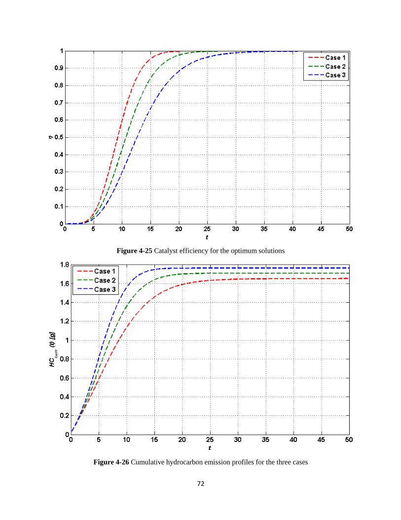
72

Figure 4-25 Catalyst efficiency for the optimum solutions

Figure 4-26 Cumulative hydrocarbon emission profiles for the three cases

73

4.4 Remarks on Using Predictive Strategies for Coldstart Control

By considering the results obtained by all of the devised predictive controlling strategies for the

engine coldstart control problem, some seminal issues regarding the pros and cons of such techniques

can be observed. As closed-loop controllers which operate based on the feedback of the real plant,

predictive controlling strategies can provide a certain level of the robustness against the existing

uncertainties and disturbances in practice, and it is expected that the calculated optimal control inputs

be reliably used for controlling the behavior of engine. This is not the case when we are using open-

loop optimal controllers, for instance PMP, which are based on the offline calculation of the

controlling commands. One of the other aspects of the simulations carried out in this chapter lies in

the fact that the considered predictive controllers have different types of objective functions and

formulations, and thus, pursuing peculiar strategies for the control of engine performance.

In particular, NMPC was developed to solve the objective function resulting from the standard

formulation of the coldstart controller, while PBNMPC was formulated to reach a desired trade-off

between the conflicting objectives at the heart of coldstart control problem, and RHSC was designed

to follow a set of the desired trajectories generated optimally in an online fashion. The results of the

simulations demonstrated the effectiveness of the proposed predictive controllers with their specific

solving procedures for real-time control applications. One of the main advantages of the proposed

predictive strategies lies in their capability to handle different types of constraints in the formulation

of control problem. Indeed, such a characteristic is often not the case when using different variants of

optimal controllers available in the literature, and thus, the utilized predictive controllers benefit from

this remarkable advantage.

However, as real-time controllers, there are some important issues concerning the implementation of

the optimization module. To be more to the point, the optimizer at the heart of optimization module

should be fast enough to result in a computationally-efficient controller suited for real-time

applications, and on the other hand, the solver should be accurate enough to calculate the near-

optimal controlling profiles to lead to a high-performance control. It is essential to take into account

such considerations for practical applications.

74

Chapter 5

Conclusions and Future Work

This chapter is presented in two sections. In the first part, the conclusions resulting from the

conducted simulations are presented. In the second section, some potential topics about the coldstart

problem which are worth for further investigations are discussed to propose some future research

directions in this area.

5.1 Conclusions

In this thesis, an extensive investigation was carried out to examine the potentials of predictive

controlling strategies for managing the performance of automotive engines over the coldstart period

to reduce the amount of cumulative tailpipe hydrocarbon emissions (HCcum). In particular, two novel

mode-based predictive controllers, namely receding horizon sliding controller (RHSC) and

preference-based nonlinear model predictive controller (PBNMPC), and also a well-known

predictive controller called nonlinear model predictive controller (NMPC) were taken into account

for the simulations.

One of the contributions of this thesis lies in the proposition of an online optimum trajectory builder

to optimally guide the controllers towards the desired trajectory. Also, different types of optimization

methods together with powerful rival optimal controllers, e.g. Pontryagin’s minimum principle

(PMP), were used to further ascertain the veracity of the devised predictive controllers. Moreover,

some novel optimization algorithms were proposed to obtain the optimum solutions in a very short

period of time to make sure that the controllers can operate in a real-time fashion.

For NMPC, the simulations indicated that the devised dynamic particle swarm optimization

(DPSO) can search the solution domain properly and yield an optimum solution in a very short

period of time. By comparing the performance of DPSO with golden search (GS) and sequential

quadratic programming (SQP), it was observed that the proposed DPSO can outperform those

powerful rival methods, at least for the coldstart control problem. Furthermore, the results of the

75

simulations clearly demonstrated that NMPC can outperform well-known classical optimal

controllers, for instance PMP.

The main motivation behind the proposition of PBMPC was the need for contriving a strategy for

having a balance between the two conflicting objectives, i.e. minimizing the engine-out hydrocarbon

emission (HCraw-c) and maximizing the exhaust gas temperature (Texh), at the heart of coldstart

controller. The method involved solving the related optimization problem based on the Tchebycheff

analysis technique, which enabled it to reach a balance between the two terms of the objective

function. The results of simulations indicated that the resulting controller can optimally balance the

conflicting objectives and reduces HCcum. Furthermore, a modified searching algorithm, known as

multivariate quadratic fit sectioning algorithm (MQFSA), was proposed to optimize the non-convex

optimization problem resulting from the Tchebycheff analysis. By comparing the performance of

MQFSA with GS and SQP, it was demonstrated that the proposed method is effective for the

coldstart optimal control design.

Finally, the performance of RHSC was evaluated for the coldstart control problem. The simulation

results indicated that combination of the sliding control and predictive control techniques can result

in a very powerful controller suited for tracking the coldstart’s desired trajectories in a real-time

fashion while satisfying a set of the system constraints. Given the promising feedback of using

MQFSA at the heart of PBMPC, the same optimization algorithm was used to calculate the optimal

commands of RHSC. The results of simulations indicated that the proposed controller can

outperform NMPC and PMP for the coldstart control problem.

To sum up, this investigation resulted in the following contributions:

Examining the potential of different variants of model-based predictive control strategies for

automotive engines HCcum reduction over the coldstart period.

Evaluating the performances of several novel techniques for solving the nonlinear optimization

problems at the heart of proposed optimal controllers, and verifying their performances through

different comparative analyses.

Proposition of a novel online optimum trajectory builder to assist the coldstart controllers perform

based on an optimum trajectory to further improve the engine performance.

76

Suggestion of novel formulations for the objective functions to achieve high-performance

predictive coldstart controllers.

5.2 Future Work

Based on the simulations carried out in this thesis, as well as detailed contemplations into the

reports of the other active research groups in this area, we realized that there are still significant

rooms for further investigations in the realm of automotive coldstart control design. In this context,

the following remarks are provided as some research topics which are worth for future studies on the

coldstart problem:

Taking advantage of adaptive controllers, and also, an adaptable version of the used control-

oriented model, to decrease the model/plant mismatch errors to boost the performances of

devised predictive controllers.

Seeking for more powerful analytical optimization algorithms for developing faster versions of

the proposed predictive control strategies.

Conducting a stability analysis to theoretically demonstrate that the devised controllers can yield

a stable system when used in practice.

Improving the structure of the presented controllers using stochastic operators to optimally deal

with the undesired effects of noises, uncertainties, and disturbances in practice.

77

REFERENCES

[1] Rajmani R (2012) Vehicle dynamics and control. Mechanical Engineering Series, Springer-Verlag.

[2] Taghavipour A, Azad NL, McPhee J (2015) Real-time predictive control strategy for a plug-in

hybrid electric powertrain. Mechatronics, doi:10.1016/j.mechatronics.2015.04.020.

[3] Ulsoy AG, Peng H, Cakmakci M (2014) Automotive control systems. Cambridge Press,

Cambridge.

[4] Zhai YJ, Yu DL (2009) Neural network model-based automotive engine air/fuel ratio control and

robustness evaluation. Eng Appl Artif Intell 22: 171–180.

[5] Taghavipour A, Azad NL, McPhee J (2012) An optimal power management strategy for power-

split plug-in hybrid electric vehicles. Int J Veh Des 60(3/4): 286–304.

[6] Asadi B, Vahidi A (2011) Predictive cruise control: utilizing upcoming traffic signal information

for improving fuel economy and reducing trip time. IEEE Trans Control Syst Technol 19(3): 707–

714.

[7] Xiao L, Gao F (2010) A comprehensive review of the development of adaptive cruise control

systems. Veh Syst Dyn 48(10): 1167-1192.

[8] Azad NL, Sanketi PR, Hedrick JK (2012) Determining model accuracy requirements for

automotive engine coldstart hydrocarbon emissions control. J Dyn Syst - T ASME 134(5): 051002.

[9] Vajedi M, Azad NL (2014) Ecological adaptive cruise controller for plug-in hybrid electric

vehicles using nonlinear model predictive control. IEEE Trans Intell Trans Syst, Accepted.

[10] Qin G, Ge A, Lee JJ (2006) Fuzzy logic control for automobiles I: knowledge-based gear position

decision. Advances in Industrial Control, pp. 145-157.

[11] Chen X, Wang Y, Haskara I, Zhu G (2014) Optimal air-to-fuel ratio tracking control with adaptive

biofuel content estimation for LNT regeneration, IEEE Trans Contr Sys Tech 22(2): 428-439.

[12] Cheng X, Jiang S, Wang S (2011) Design of a sliding mode controller for automotive engine speed

regulation, IEEE Conference Industrial Electronics and Applications, Beijing, pp. 1722-1725.

78

[13] Mozaffari A, Vajedi M, Azad NL (2015) A robust safety-oriented autonomous cruise control

scheme for electric vehicles based on model predictive control and online sequential extreme

learning machine with a hyper-level fault tolerance-based supervisor, Neurocomputing 151(2):

845-856.

[14] Salehi R, Shahbakhti M, Hedrick JK (2014) Real-time hybrid switching control of automotive cold

start hydrocarbon emission, J Dyn Syst - T ASME 136: 041002-1.

[15] Dextreit C, Kolmonovsky IV (2014) Game theory controller for hybrid electric vehicles, IEEE

Trans Contr Sys Tech 22(2): 652-663.

[16] Azad NL, Khajepour A, McPhee J (2007) Robust state feedback stabilization of articulated steer

vehicles, Vehicle Syst Dyn 45(3): 249-275.

[17] Zhang S, Zhang C, Han G, Wang Q (2014) Optimal Control Strategy Design Based on Dynamic

Programming for a Dual-Motor Coupling-Propulsion System, Sci World J 2014: Article ID:

958239.

[18] Prokhorov DV (2008) Computational intelligence in automotive applications. Studies in

Computational Intelligence, Springer-Verlag.

[19] Zavala JC (2007) Engine modeling and control for minimization of hydrocarbon coldstart

emissions in SI engine, Ph.D. Thesis, University of California, Berkeley, USA.

[20] Sanketi PR, Zavala JC, Hedrick JK (2006) Automotive engine hybrid modeling and control for

reduction of hydrocarbon emissions, Int J Control 79(5): 449-464.

[21] Wittka T, Muller V, Dittmann P, Pischinger S (2015) Development and investigation of diesel fuel

reformer for LNT regeneration, Emiss Control Sci Technol doi:10.1007/s40825-015-0017-8.

[22] Brijesh P, Sreedhara S (2013) Exhaust emissions and its control methods in compression ignition

engines: A review, Int J Auto Tech-Kor 14(2): 195-206.

[23] Shaw B, Hedrick JK (2003) Closed-loop engine coldstart control to reduce hydrocarbon emissions,

American Control Conference 1392-1397.

[24] Sanketi PR, Zavala JC, Wilcutts M, Kaga T, Hedrick JK (2007) MIMO control for automotive

coldstart. Fifth IFAC Symposium on Advances in Automotive Control, August.

79

[25] Zavala JC, Sanketi PR, Wilcutts M, Kaga T, Hedrick JK (2007) Simplified models of engine HC

emissions, exhaust temperature and catalyst temperature for automotive coldstart, Fifth IFAC

Symposium on Advances in Automotive Control, August.

[26] Mozaffari A, Azad NL, Hedrick JK (2015) A nonlinear model predictive controller for automotive

coldstart hydrocarbon emissions reduction, IEEE Trans Vehicular Technology, Submitted.

[27] Henein NA, Tagomori MK, Yassine MK, Asmus TW, Thomas CP, Hartman PG (1995) Cycle-by-

cycle analysis of HC emissions during cold start of gasoline engines, SAE Technical Paper, No.

952402.

[28] Dobner DJ (1983) Dynamic engine models for control development-Part I: Nonlinear and linear

model formulation, Int J Vehicle Des 4: 54-74.

[29] Moskwa JJ, Hedrick JK (1987) Automotive engine modeling for real-time control applications,

American Control Conference 341-346.

[30] Zavala JC, GAunther D, Sanketi PR, Willcutts M, Hedrick JK (2006) Fuel dynamics model for

coldstart, Proceedings of ASME IMECE.

[31] Sanketi PR., Azad NL, Zavala C, Hedrick JK (2008) An optimal controller formulation via convex

relaxation for automotive coldstart hydrocarbon reduction, 9th International Symposium on

Advanced Vehicle Control 312-317.

[32] Shen H, Shamim T, Sengupta S (1999) An investigation of catalytic converter performances during

cold starts, SAE Technical Paper, No. 1999-01-3473.

[33] Chan SH, Hoang DI (1999) Modeling of catalytic conversion of co/ch in gasoline exhaust at engine

coldstart, SAE Technical Paper, No. 1999-01-0452.

[34] Fiengo G, Glielmo L, Santini S, Serra G (2002) Control of the exhaust gas emissions during the

warm-up process of a TWC-equipped SI engine, 15th IFAC World Congress, Barcelona, Spain.

[35] Jones JP, Roberts JB, Pan J, Jackson RA (1999) Modeling the transient characteristics of a three

way catalyst, SAE Technical Paper, No. 1999-01-0460.

[36] Jones JP, Roberts JB, Bernard P (2000) A simplified model for the dynamics of a three way

catalytic convertor, SAE Technical Paper, No. 2000-01-0652.

80

[37] Koltsakis GC, Tsinoglou DN (2003) Thermal response of closed coupled catalysts during light-off,

SAE Technical Paper, No. 2003-01-1876.

[38] Soumelidis M, Stobart R, Jackson R (2004) A nonlinear dynamic model for three-way catalyst

control and diagnosis, SAE Technical Paper, No. 2004-01-1831.

[39] Gonatas E, Stobart R (2005) Prediction of gas concentrations in a three-way catalyst for on-board

diagnostic applications, SAE Technical Paper, No. 2005-01-0054.

[40] McNicol AC, Figueroa-Rosas H, Brace CJ, Ward MC, Watson P, Ceen RV (2004) Coldstart

emissions optimisation using an expert knowledge based calibration methodology, SAE Technical

Paper, No. 2004-01-0139.

[41] Azad NL, Sanketi PR, Hedrick JK (2012) Sliding mode control with bounded inputs and its

application to automotive coldstart emissions reduction, Invited Session on Advanced Control of

Spark Ignited Engines, American Control Conference, Montreal, Canada.

[42] Amini MR, Shahbakhti M (2014) A novel singular perturbation technique for model-based control

of cold start hydrocarbon emission, SAE International Journal of Engines, 7 (3), doi: 10.4271/2014-

01-1547.

[43] Botsaris PN, Bechrakis D, Sparis PD (2003) An estimation of three-way catalyst performance using

artificial neural networks during cold start, Appl Catal A Gen 243: 285-292.

[44] Mozaffari A, Azad NL (2014) Optimally pruned extreme learning machine with ensemble of

regularization techniques and negative correlation penalty applied to automotive engine coldstart

hydrocarbon emission identification, Neurocomputing 131: 143-156.

[45] Mozaffari A, Azad NL (2015) An ensemble neuro-fuzzy radial basis network with self-adaptive

swarm based supervisor and negative correlation for modeling automotive engine coldstart

hydrocarbon emissions: A soft solution to a crucial automotive problem, Appl Soft Comput 32:

449-467.

[46] Mozaffari A, Azad NL (2015) Coupling Gaussian generalised regression neural network and

mutable smart bee algorithm to analyse the characteristics of automotive engine coldstart

hydrocarbon emission, J Exp Theor Artif Intell 27(3): 253-272.

[47] Gray A, Ali M, Gao Y, Hedrick JK, Borelli F (2013) A unified approach to threat assessment and

control for automotive active safety, IEEE T Intell Transp 14: 1490-1499.

81

[48] Kamal MAS, Mukai M, Murata J, Kawabe T (2013) Model predictive control of vehicles on urban

roads for improved fuel economy, IEEE T Contr Syst T 21: 831-841.

[49] Maciejowski JM (2002) Predictive control with constraints. Prentice Hall.

[50] Yildiz ET, Farooqi Q, Anwar S, Chen Y, Izadian A (2012) Nonlinear constrained component

optimization for the powertrain configuration of a plug-in hybrid electric vehicle powertrain, J

Automotive Safety and Energy 3 (1): 64-70.

[51] Zou Q, Ji J, Zhang S, Shi M, Luo Y (2010) Model predictive control based on particle swarm

optimization of greenhouse climate for saving energy consumption, Word Automation Congress

123-128.

[52] Karimi J, Nobahari H, Pourtakdoust SH (2012) A new hybrid approach for dynamic continuous

optimization problems, Appl Soft Comput 12: 1158-1167.

[53] Kiefer J (1953) Sequntial minimax search for a maximum. Proc American Mathematics Society 4:

502-506.

[54] Borrelli F, Bemporad A, Fodor M, Hrovat D (2001) A hybrid approach to traction control, Hybrid

Systems: Computation and Control (Lecture Notes in Computer Science), Vol. 2034, Springer,

Berlin, 162-174.

[55] Sanketi PR (2009) Coldstart modeling and optimal control design for automotive SI engines, Ph.D.

Thesis, University of California, Berkeley, USA.

[56] Azad NL (2015) A model-based scheme for on-line optimization of automotive coldstart

hydrocarbon emission control strategy, Proc Inst Mech Eng I: J Syst Control Eng, In-Press.

[57] Chandrupatla TR (1998) An efficient quadratic fit-sectioning algorithm for minimization without

derivatives, Comput Methods in Appl Mech Eng, 152: 211-217.

[58] Hansen A, Hedrick JK (2015) Introducing the concept of receding horizon sliding control for linear

and nonlinear systems, American Control Conference.

[59] Sarpturk SZ, Istefanopulos Y, Kaynak O (1987) On the stability of discrete-time sliding mode

control systems, IEEE T Automat Contr 32 (10): 930-932.

[60] Borrelli F (2003) Constrained optimal control of linear and hybrid systems, Springer.