predictive pre-cooling control for low lift radiant...
TRANSCRIPT

Predictive Pre-Cooling Control for
Low Lift Radiant Cooling using Building Thermal Mass
by
Nicholas Thomas Gayeski
Bachelor of Arts in Physics, Cornell University (2002)
Master of Science in Building Technology, Massachusetts Institute of Technology (2007)
Submitted to the Department of Architecture
in partial fulfillment of the requirements for the Degree of
Doctor of Philosophy in Architecture: Building Technology
at the
Massachusetts Institute of Technology
September 2010
© 2010 Massachusetts Institute of Technology. All rights reserved.
Signature of author ……………………………………………………………………………………………………………………
August 6, 2010
Nicholas T. Gayeski
Department of Architecture
Certified by.…………………………………………………………………………………………………………………………………
Leslie K. Norford
Professor of Building Technology, Department of Architecture
Thesis Supervisor
Accepted by…………………………………………………………………………………………………………………………………
Takehiko Nagakura
Chair of the Department Committee on Graduate Students

2
Thesis Committee
Leslie K. Norford
Thesis Supervisor
Professor of Building Technology
Department of Architecture
Massachusetts Institute of Technology
Peter R. Armstrong
Associate Professor of Mechanical Engineering
Mechanical Engineering Program
Masdar Institute of Science and Technology
Leon R. Glicksman
Professor of Building Technology and Mechanical Engineering
Departments of Architecture and Mechanical Engineering
Massachusetts Institute of Technology

3
Predictive Pre-Cooling Control for
Low Lift Radiant Cooling using Building Thermal Mass
By
Nicholas Thomas Gayeski
Submitted to the Department of Architecture
on August 6, 2010 in partial fulfillment of the requirements for the
Degree of Doctor of Philosophy in Architecture: Building Technology
Abstract Low lift cooling systems (LLCS) hold the potential for significant energy savings relative to
conventional cooling systems. An LLCS is a cooling system which leverages existing HVAC
technologies to provide low energy cooling by operating a chiller at low pressure ratios more of
the time. An LLCS combines variable capacity chillers, hydronic distribution, radiant cooling,
thermal energy storage and predictive control to achieve lower condensing temperatures,
higher evaporating temperatures, and reductions in instantaneous cooling loads by spreading
the daily cooling load over time.
The LLCS studied in this research is composed of a variable speed chiller and a concrete-core
radiant floor, which acts as thermal energy storage. The operation of the chiller is optimized to
minimize daily energy consumption while meeting thermal comfort requirements. This is
achieved through predictive pre-cooling of the thermally massive concrete floor. The predictive
pre-cooling control optimization uses measured data from a test chamber, forecasts of
controlled climate conditions and internal loads, empirical models of chiller performance, and
data-driven models of the temperature response of the zone being controlled. These data and
models are used to determine a near-optimal operational strategy for the chiller over a 24-hour
horizon. At each hour, this optimization is updated with measured data from the previous hour
and new forecasts for the next 24 hours.
The novel contributions of this research include the following: experimental validation of the
sensible cooling energy savings of the LLCS relative to a high efficiency split system air
conditioner - savings measured in a full size test chamber were 25 percent for a typical summer
week in Atlanta subject to standard efficiency internal loads; development of a methodology
for incorporating real building thermal mass, chiller performance models, and room
temperature response models into a predictive pre-cooling control optimization for LLCS; and
detailed experimental data on the performance of a rolling-piston compressor chiller to support
this and future research.
Thesis Supervisor: Leslie K. Norford
Title: Professor of Building Technology

4
This page intentionally blank

5
Acknowledgements
This work has been supported by the Masdar Institute of Science and Technology and the Abu
Dhabi Future Energy Company. Additional funding has been drawn from the generous
donations of the Mitsubishi Electric Research Laboratory to the Building Technology program.
Thank you to the Massachusetts Institute of Technology for supporting me through the
Presidential Graduate Fellowship program and numerous teaching assistantships, and the
Martin Family for their support of sustainability research, including my own.
I am grateful and honored to have had the patient guidance of Dr. Leslie Norford, whose calm,
astute and flexible mentoring helped me find research that inspired, and whose knowledge and
advice helped it to fruition.
I am thankful for the omnipresent guidance and intellectual influence of Dr. Peter Armstrong.
His depth of knowledge and practical teaching on measurement, instrumentation, thermal
modeling, refrigeration, controls, cooling and any and all things related to buildings and energy
have been a tremendous force in my intellectual and experimental development.
Thanks to Dr. Leon Glicksman for his needed reserve and critical perspective from outside the
trenches of low-lift cooling. Your presence on the committee kept me wary of my own
assumptions and conclusions and prompted me to think clearly and think twice.
The warmest thanks to Dr. Marilyne Andersen, whose guidance through my Masters degree
and understanding and flexibility thereafter enabled me to mature and evolve as an
independent building scientist, researcher and engineer.
To Sian Kleindienst and Stephen Samouhos, thanks for being conspirators, instigators,
compatriots, and friends and to a bright future whatever may come, and whatever we create.
I extend my gratitude to all the friends, colleagues, and mentors who have helped and humored
me along the way, especially Yanni Loukissas, Saeed Arida, Josh Lobel, Zach Lamb, Brandon Roy,
Rob Darnell, Tom Pittsley, Evan Samouhos and EVCO Mechanical, Srinivas Katipamula and
PNNL, the good researchers at MERL, my friends from the Boston Architectural College and
other Solar Decathletes, my lab-mates from Building Technology, and the faculty, students and
staff of the Departments of Architecture and Mechanical Engineering. To the faculty and
students at the Masdar Institute of Science and Technology, thanks for an educational and hot
summer. To Kathleen Ross, Ali Mulcahy, and Renee Caso, thanks for all your help.
Thanks to Mom and Dad, who set the foundation and let me build. Thanks to all my family,
whose fun and emotional support bring me balance.
My love and gratitude to Celina and our dogs, for keeping me sane and driving me crazy and for
being there every step of the way.
6
Contents
List of Figures 8
List of Tables 11
Nomenclature 12
1 Introduction 14
1.1 Energy, climate and buildings 15
1.2 High performance buildings and advanced cooling systems 17
1.3 Energy monitoring, management and control 19
1.4 Thesis objectives and structure 20
2 Low-lift Cooling 22
2.1 Radiant cooling 24
2.2 Thermal energy storage and pre-cooling 27
2.3 Component mechanical systems 29
2.4 Low lift cooling systems (LLCS) 31
3. Low-lift chiller mapping and modeling 37
3.1 Low-lift compressor performance 37
3.2 Experimental assessment of low-lift heat pump performance 40
3.3 Empirical modeling of low lift heat pump performance 50
4. Thermal model identification 57
4.1 Data-drive building thermal modeling 58
4.1.1 Transfer function models 59
4.1.2 Gray-box state-space models 60
4.1.3 Black box models 61
4.1.4 Electing a temperature-CRTF inverse modeling approach 62
4.2 Experimental chamber for thermal model testing 63
4.3 Test chamber thermal model identification 71
4.3.1 Temperature-CRTF model testing 72
4.3.2 Application of temperature-CRTFs to a zone with radiant concrete
core cooling
81
4.4 Thermal model identification for LLCS 84
5. Pre-cooling control optimization 91
5.1 Predictive control with thermal energy storage and radiant systems 91
5.2 LLCS pre-cooling control objective function 93
5.3 LLCS pre-cooling control optimization 98

7
6. Low-lift Cooling Experimental Assessment 104
6.1 Description of experimental systems 104
6.1.1 Low-lift cooling system 104
6.1.2 Conventional, variable capacity split system air conditioner 113
6.1.3 Thermal inputs systems: climate chamber and internal loads 114
6.1.4 Performance measurement and instrumentation 119
6.2 LLCS test procedure 121
6.3 LLCS energy and thermal performance assessment 123
6.4 Simulating LLCS predictive pre-cooling control applied to SSAC and RCP 128
6.5 Experimental LLCS demonstration in Masdar city 132
7. Conclusion 134
7.1 Original contributions 134
7.2 Alternative LLCS configurations 136
7.3 Implementing LLCS in real buildings 139
7.5 Future research 140
7.6 Concluding remarks 142
References 143
Appendix A. Low-lift heat pump performance testing 160
A.1 Heat pump test stand sensors and instrumentation 160
A.2 Heat pump compressor inverter model 169
A.3 Low lift heat pump performance data 170
A.4 Heat pump/chiller curve-fit model coefficients 182
Appendix B. Thermal model identification testing 186
B.1 Thermal test chamber components 186
B.2 Thermal test chamber sensors and instrumentation 194
B.3 Temperature-CRTF model identification codes 198
B.4 Temperature-CRTF model coefficients 204
Appendix C. LLCS system and testing 206
C.1 LLCS and SSAC system components 206
C.2 LLCS sensors and instrumentation 207
C.3 LLCS control codes 214
8
List of Figures
Figure 1 Effect of low lift cooling technologies in achieving low pressure ratio vapor compression 23
Figure 2 Low lift cooling system operational process flow Error! Bookmark not defined.
Figure 3 Conceptual diagram of a radiant concrete-core cooling system or TABS (not to scale) 25
Figure 4 LLCS configuration energy consumption for a 'standard' performance building in five climates 34
Figure 5 LLCS configuration energy consumption for a 'medium' performance building in five climates 34
Figure 6 LLCS configuration energy consumption for a 'high' performance building in five climates 35
Figure 7 Chiller-radiant subsystem performance map based on first-principles modeling 39
Figure 8 Heat pump experimental test stand equipment component schematic 40
Figure 9 Anemometer traverse for flow measurement 41
Figure 10 Zone control volume 41
Figure 11 Heat pump experimental test stand 41
Figure 12 Data acquisition system and sensors 41
Figure 13 Range of pressure ratios spanned by 131 test conditions 43
Figure 14 Heat pump experimental test stand sensor schematic 44
Figure 15 Condenser air flowrate as a function of fan speed 45
Figure 16 Condenser fan power consumption as a function of fan speed 45
Figure 18 Efficiency of the inverter supplying the compressor and the compressor isentropic efficiency 46
Figure 17 Compressor and outdoor unit (including condenser fan and electronics) electric input ratio, kW
electricity consumed per kW cooling delivered, and coefficient of performance COP, kW cooling
delivered per kW of electricity consumed as a function of pressure ratio 46
Figure 19 Steady-state energy balance validation 48
Figure 20 Steady-state mass flow rate discrepancies expressed as deviations of each of the three inferred
mass flow rates from their average at each test condition 48
Figure 21 Validation of Curve Fit Cooling Capacity Model 54
Figure 22 Validation of Curve Fit Power Model 54
Figure 23 Validation of Curve Fit EIR Model 54
Figure 24 EIR as a function of compressor speed for combinations of Tz = 15, 20 and 25 C and Tx = 20, 30 and
40 C at condenser fan speeds of 300, 700, and 1100 RPM 55
Figure 25 EIR as a function of condenser fan speed for combinations of Tz = 15, 20 and 25 C and Tx = 20, 30
and 40 C at compressor speeds of 20, 50 and 80 Hz 56
Figure 26 Experimental chamber constructions and dimensions 66
Figure 27 Experimental test chamber with convective heater (white box), radiant ceiling panels (wire mesh
above), and radiant floor heating (below concrete) 67
Figure 28 Experimental test chamber with radiant concrete floor loop, before installation of the concrete
layers 67
Figure 29 Experimental chamber thermocouple locations (dimensions listed in Appendix B.2) 68
Figure 30 Measured temperature response and heat rates for model identification testing with three layers of
pavers, including climate chamber temperature excitation, internal convective heat input, internal
radiant heat input, and radiant concrete floor heating 69
Figure 31 Measured temperature response and heat or cooling rates for application of model identification to
a concrete floor cooling system with three layers of pavers. Cooling is delivered through a chilled
water loop underneath the concrete layers 70
9
Figure 32 Star network for approximating radiative and convective heat transfer between wall surfaces and
the zone air from [Seem 1987] where T1-3 are wall surface temperatures, q1-3 are net heat transfer
rates into the wall surface, R1-3 are resistances to an intermediate temperature node Tstar, R is the
resistance between the intermediate temperature and the room temperature Tr and qload is the
zone cooling load 73
Figure 33 Accuracy of inverse model on training data. The top two graphs show a sample of training data for
a floor heating test. The bottom three graphs show the inverse model's accuracy in predicting zone
air temperature (ZAT), mean radiant temperature (MRT) and operative temperature (OPT). The
RMSEs presented are for the entire training data set, including five sets of training data in addition
to that shown 77
Figure 34 Accuracy of inverse model for floor heating validation data. 78
Figure 35 Accuracy of inverse model for convective heating validation data 79
Figure 36 One-step ahead prediction RMSE for zone operative temperature (OPT) for training data (top) and
validation data (bottom) as a function of the time interval for sampling data and the order of the
temperature-CRTF model 80
Figure 37 Concrete-core radiant floor cooling temperature-CRTF model one-step ahead training data
prediction RMSE for ZAT, MRT, OPT, UST, and RWT 85
Figure 38 Concrete-core radiant floor sample validation data temperature inputs, thermal inputs, and
temperature outputs 86
Figure 39 Concrete-core radiant floor cooling temperature-CRTF model 24-hour-ahead validation data
prediction RMSE for ZAT, MRT, OPT, UST, and RWT 87
Figure 40 Concrete-core radiant floor cooling temperature-CRTF model 96-hour-ahead validation data
prediction RMSE for ZAT, MRT, OPT, UST, and RWT 88
Figure 41 Concrete-core radiant floor OPT temperature-CRTF model one-step-ahead RMSE as a function of
sampling interval and model order for training data (top) and validation data (bottom) 89
Figure 42 Concrete-core radiant floor OPT temperature-CRTF model 24-hour-ahead RMSE as a function of
sampling interval and model order for validation data 90
Figure 43 RWT prediction error with 30 minute sampling as a function of transfer function model order,
corresponding to the order of the thermal network between the UST and RWT measurements. 90
Figure 44 Operative temperature penalty term �PENOPT 97
Figure 45 Pattern search optimization algorithm flow chart 100
Figure 46 Closed loop optimization of compressor speed 101
Figure 47 Sample pattern search results, including predicted OPT, RWT, and UST over a 24 hour look ahead
(top left), cumulative energy consumption (top right), chiller power consumption at each half hour
(bottom left), and predicted optimal compressor speed at each hour (bottom right) 103
Figure 48 Low-lift cooling system: variable capacity chiller 106
Figure 49 Low-lift cooling system: radiant floor water loop 106
Figure 50 Superheat control set point vs compressor speed 107
Figure 51 Offset in chiller capacity (top), power consumption (middle) and COP (bottom) for the modified
chiller 110
Figure 52 Condenser, condenser fan and compressor (normally the electronics, including the compressor
inverter, is cooled by the condenser air stream) 111
Figure 53 Two refrigerant loop branches serving the air -side indoor unit and the BPHX. The plant-side chilled
water loop is also shown 111
Figure 55 Complete LLCS radiant concrete-core floor test chamber 112

10
Figure 54 Chilled water loop distribution, including radiant floor manifold, PEX pipe loops, Warmboard sub-
floor. The air-side indoor unit evaporator is also shown. 112
Figure 56 Split-system variable capacity air conditioner that uses the same outdoor unit as the LLCS 113
Figure 57 Typical summer week hourly outdoor air temperature (OAT) schedule for Atlanta and Phoenix 116
Figure 58 Lighting, simulated equipment and occupant loads 117
Figure 59 Internal load schedule for standard efficiency and high efficiency loads 117
Figure 60 Comparison of refrigerant side and chilled water side cooling rate measurement CHANGE RMSE to
CV-RMSE 119
Figure 61 Low lift chiller system performance measurement instrumentation 120
Figure 62 Results for the LLCS under Atlanta climate and standard loads. For the duration of the test, the top
graph shows the outdoor air temperature (OAT), adjacent zone air temperature (AAT), zone
operative temperature (OPT), under-slab temperature (UST) and return water temperature (RWT);
the middle graph shows the internal load heat rate and the cooling rate; and the bottom graph
shows the LLCS power consumption at each hour. 124
Figure 63 Results for the SSAC under Atlanta climate and standard loads. For the duration of the test, the top
graph shows the outdoor air temperature (OAT), adjacent zone air temperature (AAT), zone
operative temperature (OPT), under-slab temperature (UST) and return water temperature (RWT);
the middle graph shows the internal load heat rate and the cooling rate; and the bottom graph
shows the LLCS power consumption at each hour. Note: the cooling rate measurement does not
include cooling during transient conditions, which are significant, because the refrigerant mass flow
rate used for calculating QC was not measureable during transient conditions. (This is typical of
Coriolis mass flow meters with significant two phase flow) 125
Figure 64 Comparing zone operative temperatures (OPT) for the LLCS and split system AC operation 127
Figure 65 Images of the Masdar City experimental LLCS demonstration project, including the underslab
insulation and PEX chilled water pipe (top left), the variable capacity chiller (top right), the project
site and the three LLCS modules (bottom left), and the poured concrete floor (bottom right). 131

11
List of Tables Table 1 Building component performance levels used in [Armstrong et al 2009b] 32
Table 2 LLCS energy savings relative to DOE benchmark by building type across 16 climates 35
Table 3 Heat pump experimental test stand sensor descriptions 44
Table 4 Experimental test chamber construction layers 66
Table 5 Thermocouple label terminology 68
Table 6 Internal load distribution and density 117
Table 7 Low lift chiller system sensor labels 120
Table 8 Comparison of SSAC and LLCS performance 126
Table 9 Energy consumption and relative savings from simulations of SSAC, TABS and RCP under with low-lift
predictive pre-cooling control 130

12
Nomenclature
AAT Adjacent zone air temperature
AHU Air handling unit
ANN Artificial neural network
ARMAX Auto-regressive, moving average with exogenous variables model
ASHRAE American Society of Heating, Refrigerating and Air Conditioning Engineers
BAS Building automation system
BPHX Brazed plate heat exchanger
BTU British thermal units
C Celsius
CFD Computational fluid dynamics
CFM Cubic feet per minute
COP Coefficient of performance
CRTF Comprehensive room transfer function
CTF Conduction transfer function
DOAS Dedicated outdoor air system
DOE United States Department of Energy
EER Energy efficiency ratio
EIR Electric input ratio, the reciprocal of COP
EMCS Energy management and control system
EPW EnergyPlus weather file
EVT Evaporating temperature
f Condenser fan speed
GtCO2-eq/yr Gigatons of carbon dioxide equivalent per year
GPM Gallons per minute
H Enthalpy
HPB High performance building
HVAC Heating, ventilating and air conditioning
Hz Hertz
IPLV Integrated part load value
K Kelvin
kPa Kilopascals
kW Kilowatts
kWh Kilowatt-hours
LLCS Low lift cooling system
LLCS-SSAC Low lift cooling system applying predictive control to a SSAC
LLCS-TABS Low lift cooling system with a thermo-active building system
LLCS-RCP Low lift cooling system using radiant ceiling panels and passive TES
m& Mass flow rate
MIST Masdar Institute of Science and Technology
MIT Massachusetts Institute of Technology
MRT Mean radiant temperature

13
NARX Nonlinear autoregressive with exogenous variables model
OAT Outdoor air temperature
OPT Operative temperature
P Power (or Pressure)
Pt System power consumption at time t
PID Proportional-Integral-Derivative control law
PCM Phase change material
PENEVTt Evaporating temperature penalty function at time t
PENOPTt Operative temperature penalty functionat time t
PEX Polyethylene pipe
PLR Part load ratio
PNNL Pacific Northwest National Laboratory
QC Cooling rate
QI Internal load heat rate
RC Resistance and capacitance (in a thermal RC network)
R410A Refrigerant R410A, consisting of 50 percent R-32 and 50 percent R125
RCP Radiant ceiling panel
RMSE Root mean square error
RPM Revolutions per minute
RTU Rooftop unit HVAC system
RWT Chilled water return temperature
SEER Seasonal energy efficiency ratio
Sqft Square feet
SSAC Split system air conditioner
T Temperature
TABS Thermo-active building systems (concrete-core heating and cooling)
TCs Thermocouples
TES Thermal energy storage
TMY Typical meteorological year
TOU Time-of-use electricity rate
UA Total thermal conductance in W/K
UAE United Arab Emirates
UST Under-slab temperature (at the bottom of the concrete slab)
VAV Variable air volume heating, cooling and ventilation system
VSD Variable speed drive
W Watts (or power)
Wh Watt-hours
" Volumetric flowrate
ZAT Zone air temperature
∆T Temperature difference
ω Compressor speed
� Operative temperature penalty weight in W/K2

14
Chapter 1 Introduction
Consumption of energy through buildings and its impact on climate and environment have
motivated a broad effort to seek practical and innovative energy efficiency and conservation
measures for buildings. Globally, between 30 and 40 percent of primary energy consumption is
through buildings [UNEP 2007]. In the U.S., around 39 percent of national primary energy
consumption is through buildings and its share is projected to increase in the next twenty years
[USDOE 2006]. Improved building design, retrofits of existing buildings, better lighting, efficient
heating, ventilation and air conditioning (HVAC), improved control, more efficient appliances,
better operations and maintenance, and numerous other approaches hold immediate potential
for energy savings [McKinsey 2007]. The barriers to progress on these measures are largely
systemic issues in the industry, primarily rooted in lack of education, lack of incentive, or lack of
requirement through codes [Granade et al 2009].
In the long-term, there is a deeper need for new ideas and new strategies to further and
prolong energy efficiency and conservation gains in buildings. In a recent report, “Unlocking
Energy Efficiency in the U.S. Economy”, McKinsey and Company stated as one of its five
overarching strategies the need to “Foster innovation in the development and deployment of
next-generation energy efficiency technologies to ensure ongoing productivity gains” [Granade
et al 2009]. In other words, to sustain and further efficiency gains achievable with current
technology and practices, new technologies and strategies will be required for sustainable
global development. In buildings, this could mean anything from new tools for improved
designs, new methods to achieve more economical retrofits, new technologies to improve
performance, or new processes to improve operations and maintenance.
This research looks ahead from existing practices and trends in HVAC design, operation,
monitoring and control towards an integrated approach to designing and operating a coupled
passive and active cooling strategy with more intelligent control using measured building data.
This strategy is called low lift cooling. Low lift cooling refers broadly to cooling strategies that
leverage existing HVAC technologies to operate chillers at low pressure ratios more of the time,
thereby enabling significant cooling energy savings. Typically, low lift cooling systems (LLCS)
combine variable capacity chillers, hydronic distribution, radiant cooling, thermal energy
storage (TES) and predictive pre-cooling control to achieve lower condensing temperatures and
higher evaporating temperatures, resulting in higher average chiller efficiency and energy
savings. [Armstrong et al 2009a, Armstrong et al 2009b, Jiang et al 2007, Katipamula et al 2010].

1. Introduction
15
In this research, an experimental LLCS was developed, built and tested consisting of a variable
capacity chiller serving a concrete radiant floor, similar to a thermo-active building system
(TABS) in which chilled water pipes are embedded in the concrete slab of a building. Predictive
control of the chiller was implemented to pre-cool the radiant concrete floor in anticipation of
future cooling loads based on forecast climate and internal loads. Models of chiller
performance and zone temperature response were identified from measured data and used to
inform the predictive control algorithm. Finally, the energy and thermal comfort performance
of the LLCS was compared to the performance of a high efficiency split system air conditioner
(SSAC) subject to the same climate conditions and internal loads.
1.1 Energy, climate and buildings
Society’s approach to and perspective on energy, climate and buildings are interdependent.
Regardless of one’s views on climate change, energy has become a premier challenge for the
21st century and beyond. The potential for political instabilities, local environmental impacts,
increasing costs, and rising demand for energy-intensive services make energy a primary
national and international priority. For those who find the uncertainties in climate change
science - role of oceans, aerosols, clouds, etc - to be outweighed by the evidence for
anthropogenic causes of climate change and potential adverse impacts, tackling the energy
problem is even more crucial to the future of our societies.
Among these two mammoth issues, energy and climate, lies the challenge of buildings. All too
often a discussion about energy and climate conjures up images of billowing smokestacks from
massive power plants or industrial facilities, backed up traffic on urban highways, or oil spills
from offshore drilling rigs or international tankers. All too infrequently does the discussion turn
to the pervasive presence of lighting, building heating and cooling, ventilation, appliances and
other auxiliary building loads that dominate energy and electrical power consumption in
modern life. These building-related loads constitute the majority of energy and electric
consumption throughout modern, industrialized nations. There has been a giant white
elephant in the room of national energy policy for decades that energy efficiency, and
especially energy efficiency in buildings, is critical towards creating a better energy policy and
infrastructure.
Numerous scientists, policy-makers, and engineers have pointed towards energy efficiency and
‘soft’ energy technologies as a solution to energy and climate problems. Amory Lovins, in his
well-known 1976 Foreign Affairs article pointed to a soft path for energy policy. The soft path
employs energy efficient technologies for appliances, HVAC and lighting, renewable energy
sources, and transitional technologies for fossil fuel generation to move away from dependence
on oil, gas, coal, and nuclear sources of energy [Lovins 1976]. Lovins’ observations are still
relevant today. David Goldstein, Art Rosenfeld, and other efficiency advocates spent decades
working for appliance efficiency standards. Their efforts have not been in vain. Estimates
suggests that decades of improvements in refrigerator appliance standards have saved over 17
billion dollars [Goldstein 2007] as average refrigerator energy consumption dropped from 1800
kWh/year to 450 kWh/year between 1977 and 2002.

1. Introduction
16
This deliberate, long-term and persistent approach to achieving energy savings through energy
efficiency standards reaps real rewards. In the buildings sector in the United States, building
energy codes have been the primary regulatory tool for driving efficiency. However, turnover
in the building stock is very slow, and codes lag far behind state of the art technology. Driving
significant building energy savings in the United States will require both aggressive retrofitting
of the existing building stock and the construction of low-energy or even zero net-energy
buildings. Creating new, low energy best available technologies to motivate more aggressive
energy efficiency standards is an important path to improving building energy efficiency. LLCS
constitute one of these potential low energy technologies.
Reducing greenhouse gas emissions in the United States will also require a sharp focus on
building-related carbon dioxide emissions. McKinsey estimates that many of the least cost
carbon dioxide abatement measures relate to creating better buildings. LED lighting, façade
renovations, building controls, co-generation, HVAC equipment improvements and other
building and appliance efficiencies make up over 50 percent of the carbon dioxide abatement
potential [McKinsey 2007].
Internationally, the intergovernmental panel on climate change (IPCC) estimates that the
buildings sector holds the potential for reduction of 5.3 to 6.7 Gigatons of CO2 equivalent per
year (GtCO2-eq/yr) at less than $100/tCO2-eq [Levine et al 2007]. That is the largest potential
among all sectors. The technical solutions referenced by the IPCC are many, including passive
façades, integrated design, more efficient mechanical systems, leveraging thermal mass, better
commissioning and fault detection, and building energy management systems. The barriers are
also many, including poor short term cost/benefit analyses, split incentives, hidden costs,
perceived risk, and organizational ignorance or inertia [Levermore 2008, Levine et al 2007].
One of the greatest challenges is that most of the energy reductions will be required in existing
buildings.
For new construction, particularly in developing countries where construction and development
continues at a rapid pace, applying the best design and technologies to minimize energy
demand in new buildings is a major priority. The Energy Information Administration (EIA)
estimates a 34 percent increase in building energy consumption in 20 years [Perez-Lombard
2007]. At the same time, the IPCC working group on residential and commercial buildings
estimates that new buildings could potentially consume one quarter of the energy of a typical
existing building [Levine et al 2007]. Integrated design, passive reduction of building loads,
highly efficient cooling and ventilation, and building energy management systems all make the
short list of technical solutions to reduce the growth of energy consumption in new buildings.
New building construction generally involves more cooling than in the past and higher demand
for thermal comfort. As such, efficient cooling is rapidly becoming a critical issue for energy
efficient buildings. In the United States, space cooling accounts for around 12.6 percent of the
total primary energy consumption in commercial buildings [USDOE 2006], and demand for
cooling continues to grow in the U.S. and abroad. In Europe, it has been estimated that the air
conditioned floor area will increase from 2,100 to 3,300 billion square meters by 2020 [Brunner

1. Introduction
17
et al 2006], increasing electric demand from 102 to 159 TWh per year for cooling. Furthermore,
in other areas of the world cooling is or will be an even more significant fraction of energy
consumption. Much of the developing world, where urbanization and building construction are
fastest, is located in lower latitudes where the need for cooling is greater.
Sivak [2009] analyzed the potential growth in cooling energy demand in the 50 largest
metropolitan areas in the world. This analysis showed that 38 of the largest 50 metropolitan
areas are in developing countries, where building construction and demand for thermal
comfort and HVAC are on the rise. Of these 38, 24 have greater cooling demands than heating
demands. Sivak estimated that if cooling was provided at the same level as that in the United
States, the cooling demand in Mumbai, India with a population of just 13.8 million would be
equivalent to 24 percent of the cooling demand for the entire United States. Complicating
matters further, Degelman [2002] projected that cooling energy loads would significantly
increase in low and middle latitude cities as a result of climate change.
The need for reliable and secure energy, the impacts on climate and environment,
development in cooling dominated climates, and the rising demand for cooling and comfort
motivate a need for highly efficient mechanical cooling systems coupled with reduced building
thermal loads through better design. The next chapter will discuss technical strategies to meet
this need through highly efficient, high performance buildings and advanced cooling strategies.
1.2 High performance buildings and advanced cooling systems
There are many technologies, design options and operational strategies available to reduce the
energy consumption of buildings. A high performance building (HPB) is a term broadly used to
define buildings that perform better than conventional buildings. The American Society of
Heating, Refrigerating and Air Conditioning Engineers’ (ASHRAE) Standard 189.1, the Standard
for the Design of High Performance Green Buildings, defines an HPB as:
“a building designed, constructed and capable of being operated in a manner that
increases environmental performance and economic value over time, seeks to establish
an indoor environment that supports the health of occupants, and enhances the
satisfaction and productivity of occupants through integration of environmentally
preferable building materials and water-efficient and energy-efficient systems”.
[ASHRAE 2009]
In simple terms, high performance buildings are buildings that provide a better environment for
occupants, better economic value, lower energy consumption, lower water consumption, and
lower life-cycle costs.
There are numerous resources available describing how to create high performance buildings.
ASHRAE standard 189.1 provides minimum requirements for the “siting, design, construction,
and plan for operation of high performance green buildings” [ASHRAE 2009]. However,
ASHRAE 189.1 requirements largely reflect just a step above the standard state of the art, as

1. Introduction
18
outlined in ASHRAE 90.1, the Standard for the Energy Performance of Buildings [ASHRAE
2007c].
Going beyond standard systems with high efficiency equipment enables even greater energy
savings, but often requires a more integrated and innovative approach to both building and
mechanical design, construction, control and operation. Integrated design processes seek to
include architects, engineers, building owners, commissioning agents, and construction
managers early in the process of creating a building to facilitate better design and coordinated
strategies [Lewis 2004]. In terms of energy efficiency, the intent of this integrated design
approach is to coordinate building siting, form, and envelope with passive lighting, thermal,
ventilation, and mechanical system strategies to create a highly energy efficient and economical
building.
Reducing energy consumption and providing a comfortable environment to occupants are the
two important aspects of HPB with relation to this research. Managing the impact of
environmental conditions on thermal loads and lighting through passive design are the first
steps towards these goals. Strategies such as effective siting and orientation of a building can
reduce solar loads, provide better access to light, and enhance natural ventilation. Façade
design and building envelope optimization can further provide shading, reduce heat transfer
across the envelope, and provide for the implementation of passive cross-ventilation or
buoyancy-driven natural ventilation strategies.
Reducing internal loads due to office equipment, lighting, and auxiliary equipment are doubly
important. This strategy reduces electrical loads directly, but also reduces the thermal load and
subsequent demands on HVAC equipment. Combined with proper passive thermal
management, reducing equipment internal loads can lead to operational cost and capital cost
savings through reductions in the size of mechanical equipment [Todesco 2004].
Integrating passive ventilation strategies with efficient mechanical ventilation and conditioning
can further reduce energy consumption. Providing mixed mode ventilation systems that allow
for natural ventilation or night ventilation under favorable conditions can offset the need to use
mechanical equipment. The greatest reduction in HVAC energy and costs is often achieved by
avoiding the need for mechanical HVAC systems altogether, sometimes or all of the time.
There are a plethora of efficient active mechanical system components currently in use in HPB.
Condensing boilers, variable speed chillers, variable speed pumps and fans, energy and
enthalpy recovery systems, TES, radiant systems, and dedicated outdoor air systems are some
of the many technologies being deployed to achieve energy efficiency. An efficient overall
system however, arises from the design, proper construction, commissioning, effective control,
and appropriate operation and maintenance of a combination of these components in an
integrated manner. As will be discussed in chapter 2, this research draws from this principle
that existing high efficiency mechanical components can be integrated into a highly efficient
system, an LLCS, so that drastic energy savings are achieved.

1. Introduction
19
There are numerous examples of HPB with highly efficient systems leveraging passive design,
natural ventilation and high efficiency mechanical equipment to provide cooling. Actuated
façade systems providing natural ventilation have been employed in buildings such as the San
Francisco Federal Building. Buoyancy-driven natural ventilation has been employed in such
buildings as Lanchester Library or the Queen’s Building at De Montfort University in England.
Another approach is to mix active and passive strategies. Mixed-mode systems use natural
ventilation for part of the building and/or part of the time but mechanical systems under
conditions unfavorable for natural ventilation or during peak loads. Buildings such as the Kirsch
Center for Environmental Studies or the California Academy of Sciences are naturally ventilated
but with radiant concrete slabs which provide cooling under peak load conditions [McConahey
2008].
In many climates, passive strategies and natural ventilation alone cannot provide thermal
comfort. If mean temperatures, and especially night-time mean temperatures, are outside of
the desired range for thermal comfort it will not be possible to naturally ventilate during the
day or at night. In addition, practical issues such as outdoor air quality or street noise may be
prohibitive to naturally ventilating a building. In these cases, efficient mechanical systems are
necessary to provide cooling for adequate thermal comfort.
Many technologies are available for active low-energy cooling strategies. Thermally driven heat
pumps, such as absorption, adsorption or chemisorption heat pumps [Oxizidis and
Papadopolous 2008], can be incorporated into systems where waste heat or solar thermal
energy is available. Variable speed chillers combined with variable speed distribution systems
provide low energy chilled water generation and distribution. Coupling these with chilled
beams, chilled ceiling panels, or radiant concrete-cores can eliminate fan energy and raise the
chilled water temperature setpoint, improving chiller efficiency. TES can be employed to shift
loads from peak demand periods to the nighttime. This has the additional benefit of chiller
operation at lower condensing temperatures. Recent attention has been given to a TES
strategy called thermo-active building systems (TABS) in which chilled water pipes are
embedding in the concrete slab of every floor of a building [Lehman et al 2007]. With TABS the
building concrete structure can be pre-cooled, providing cooling to building spaces later in the
day due to the thermal time lag of the concrete.
The details of these specific advanced cooling technologies, radiant cooling, TES with
precooling, variable capacity chillers and hydronic distribution are discussed in chapter 2.
1.3 Energy monitoring, management and control
The final broad trend in the building industry influencing this research is the increasing
availability and utility of building data. The revolution in information technology in the past
thirty years is still only beginning to impact the building sector. To date, major changes include
the emergence of direct digital control systems, networked building systems and components,
centralized control through building automation systems (BAS), and opportunities for energy
efficiency and optimization through energy management and control systems (EMCS).

1. Introduction
20
Networked building systems with centralized controls are slowly becoming the norm for large
new construction projects and renovations. Today, monitored data from buildings can be used
to perform data-driven modeling, analysis, simulation, benchmarking, fault detection,
optimization and supervisory control to improve the performance and operation of buildings
[Motegi et al 2003, Brambley et al 2005, Roth et al 2005].
Opportunities still just emerging for building energy management and control include optimal
whole building control systems, simulation based control and optimization, and model-based
predictive control. Optimal model-based predictive control is premised on the notion that
data-driven or physically based models of buildings can be created using monitored building
data, and that these models can be used to determine the most energy efficient or cost
effective control strategies [Quartararo 2006, Hatley et al 2005]. Some optimal control
algorithms use parametric models of building systems created from known engineering
quantities using simulation tools [Kolokotsa et al 2005, Clarke et al 2002, Mahdavi 2001, Henze
and Krarti 2005]. Another approach is to use monitored building data to train data-driven
models from measured building performance. This approach has been explored by [Braun and
Chaturvedi 2002, Armstrong et al 2006a, Armstrong et al 2006b]. This thesis will follow a
similar approach in implementing a model-based predictive control strategy, as described in
chapters 4 and 5.
1.4 Thesis objectives and structure
The confluence of issues around energy, climate and buildings, new technologies for low-
energy cooling, and the emerging role of building data in achieving efficiency provide a broad
context for this work. This research seeks to advance the art of a low-energy cooling strategy,
LLCS, which leverages building monitoring and control systems to greatly improve energy
efficiency. The ultimate goals are to drastically reduce the energy consumption required for
cooling buildings, scale down building energy demands to make building integrated power
feasible, and reduce the environmental and climate impacts of buildings.
Advancing low-lift cooling requires both theoretical development and experimental testing with
variable speed chillers, radiant concrete-core cooling, radiant panel cooling, dedicated outdoor
air systems (DOAS), TES, thermal model identification, pre-cooling control optimization, and
model-based control. This dissertation offers original contributions on the following key issues:
• A performance comparison of an LLCS cooling system with predictive pre-cooling control
to a high efficiency SSAC.
• Development of a pre-cooling optimization control algorithm for LLCS that incorporates
the transient response of real building thermal mass. This algorithm determines a near-
optimal chiller control schedule using outside temperature and internal gain forecast,
chiller performance models, and building temperature response models.
• Measurement and empirical modeling of the performance of a rolling piston compressor
heat pump/chiller over a wide range of pressure ratios including low pressure ratios.
1. Introduction
21
• Application of building thermal model identification methods to the problem of passive
pre-cooling control optimization for concrete core radiant cooling.
The dissertation will conform to the following structure:
Chapter 2 will be a literature review of the most important research underpinning LLCS.
Research on radiant cooling and pre-cooling of TES will be reviewed in detail. Prior research on
low-lift cooling, its constituent systems and supporting strategies will be explained.
Chapter 3 will explain experimental research to characterize the performance of a variable
speed heat pump/chiller at low pressure ratios. This will include a review of prior research on
chiller performance at low-pressure ratio, an explanation of the experimental apparatus and
procedure for measuring heat pump/chiller performance under low-pressure ratio conditions,
and presentation of empirical curve-fit models to represent chiller performance as a function of
chilled water return temperature, outdoor air temperature, compressor speed and condenser
fan speed.
Chapter 4 will focus on thermal model identification methods and results for predicting zone
temperature response. It will review prior research on thermal model identification. Thermal
model identification methods will be applied to predicting the thermal response of a thermally
massive test chamber.
Chapter 5 will discuss the development of a pre-cooling control optimization algorithm for
predictive control of the variable speed chiller. The empirical performance maps and data-
driven zone temperature response models developed in chapters 3 and 4 are integrated into
the optimization objective function. Compressor and condenser fan speeds can be set hourly to
determine the optimal chiller dispatch schedule that will minimize power consumption and
maintain thermal comfort.
Chapter 6 will detail the results of designing, building and implementing control over an
experimental LLCS consisting of a variable capacity chiller serving a concrete-core radiant
cooling system with predictive control. The energy and thermal comfort performance of the
system will be compared to a high efficiency, variable capacity SSAC with a seasonal energy
efficiency ratio (SEER) of 16 BTU/Wh. Simulations will be performed to compare LLCS
performance to SSAC with conventional thermostatic control and with predictive control.
Chapter 7 will conclude with a summary of the original contributions of this research and its
results. A summary of alternative LLCS strategies will be reviewed along with barriers and
benefits to applying LLCS on a broad scale. Finally, future LLCS research needs will be
presented.

22
Chapter 2 Low Lift Cooling Systems Low-lift cooling systems (LLCS) hold promise for dramatically more efficient cooling of buildings.
As previously explained, an LLCS is a cooling system that leverages existing HVAC technologies
to operate vapor compression chillers at low pressure ratios more of the time while still
meeting human thermal comfort standards. LLCS are typically made up of a few key HVAC
components and strategies that enable low pressure ratio operation. These include variable
speed compressors, hydronic distribution with variable speed pumps, radiant cooling, TES,
predictive pre-cooling control, and dedicated outdoor air systems.
A temperature-entropy (T-S) diagram of a vapor compression cycle and the effect of each HVAC
technology in an LLCS are shown in
Figure 1. The larger polygon on the T-S diagram represents typical air-cooled chiller operation
with low chilled water temperature and high, daytime condenser air temperatures. The smaller
polygon on the T-S diagram represent low lift chiller operation with radiant cooling, variable
speed hydronic distribution, TES, predictive pre-cooling control, and a variable capacity chiller.
The use of radiant cooling and variable speed pumping allow for high chilled water
temperatures and higher evaporating temperatures. Pre-cooling of TES overnight or in the
early morning allows the chiller to operate when outdoor temperatures are lower, leading to
lower condensing temperatures. Variable capacity chillers with variable speed compressors
allow the chiller to modulate capacity in response to cooling load.
The cooling provided by both of these cycles is represented by the area under the bottom line
of the vapor compression cycle. The work required to operate the vapor compression cycle is
represented by the area inside the polygons. This diagram shows why chillers can operate
more efficiently at low lift conditions. The LLCS can produce a similar (or greater) cooling effect
as the conventional system while requiring less work. As a result, a chiller operated at low lift
has a higher coefficient of performance (COP) than under typical conditions, with subsequent
energy savings.

2. Low lift cooling systems
23
Figure 1 Effect of low lift cooling technologies in achieving low pressure ratio vapor compression
Figure 2 Low lift cooling system operational process flow

2. Low lift cooling systems
24
Figure 2 shows a conceptual diagram of how LLCS work. Starting at the top of the diagram,
forecasts of internal loads, temperature, and solar conditions along with measured building
data are gathered and delivered to a building control system (the computer in the diagram).
Thermal model identification is performed on the building data to train a model of zone
temperature response as a function of building loads and cooling rate input. Using this model,
and a model of cooling system energy consumption, a near-optimal control schedule is
determined for the chiller which may include pre-cooling of active TES, pre-cooling of thermo-
active building systems (TABS), or direct cooling of a space.
Estimated energy savings of LLCS over typical variable air volume (VAV) systems common in the
United States with conventional two-speed chillers are large. For typical buildings, cooling
energy savings range from 37 to 84 percent depending on the climate [Katipamula et al 2010].
In high performance buildings, savings range from -9 to 70 percent of cooling energy
consumption. The low end demonstrates that LLCS may not be attractive for high performance
buildings in mild climates where free cooling through economizers is available. Although low-
lift cooling is a relatively new concept from a systems integration viewpoint, the component
cooling strategies, constituent systems and pre-cooling control strategies have a long history of
research, development and implementation.
This chapter will provide a literature review of research relevant to LLCS. These include radiant
cooling, pre-cooling TES, mechanical system components such as variable speed chillers, pumps
and fans and dedicated outdoor air systems. Existing LLCS research will also be reviewed.
2.1 Radiant cooling
Radiant cooling is strategy by which cold surfaces absorb heat from objects (such as people),
surfaces and air in a room through radiative, and to a lesser extent convective, heat transfer.
Typically radiant systems consist of low thermal mass radiant panels, or thermally-massive
radiant concrete-cores which have chilled water pipes embedded in concrete, or TABS. Radiant
cooling enables energy savings primarily through three mechanisms. First, air temperatures in
a zone can be warmer as the operative temperature is lowered by cool radiant temperatures.
Second, transport energy for pumping chilled water is lower than fan energy for all-air systems.
Third, chilled water temperatures, and thus evaporating temperatures, are higher which
reduces the burden on the chiller. Although radiant cooling systems have been installed in
many buildings, it is still an emerging technology. There is ongoing research on how best to
integrate and control radiant systems of different types, in different climates, with different
companion systems, and with TES [Braun et al 2001, Vangtook and Chirarattananon 2006,
Armstrong et al 2009b, Roth et al 2009]. This section will review the current state of research
on radiant cooling, a major sub-component of a LLCS.
The potential benefits of radiant cooling systems are many, including reduced energy
consumption, improved air quality and humidity control, reduced space requirements, and
potentially even lower first costs [Feustel and Stetiu 1995]. Radiant cooling operates through
large, cooled surfaces which absorb radiant energy from a space, with some convective cooling

2. Low lift cooling systems
25
as well. Because radiant systems include a large, cool surface inside a zone humidity control
must be provided separately to prevent condensation. Radiant systems also do not provide
ventilation air. Typically, radiant cooling systems are combined with small ventilation systems
that provide latent cooling and ventilation air. Higher potential costs, condensation,
remodeling constraints, and architectural design freedom all pose real or perceived threats to
the applicability of radiant cooling [Engineered Systems 2002].
Olesen [1997] explained design considerations for radiant floor cooling systems, including
radiant concrete-core cooling or TABS, a conceptual diagram of which is shown in Figure 3.
Typical radiant floor cooling systems require tube spacing between 75 and 300 mm to achieve
adequate cooling capacity, although floor covering, slab thickness and slab thermal properties
are also important considerations in design. Olesen et al [2003] describe European standards
for designing radiant concrete-core cooling systems including calculation of heat transfer
between chilled water and the zone based on pipe type and spacing, concrete characteristics
and flow rate. Olesen et al [2000a] describes the calculation of the heat exchange coefficient
between the floor surface and a space, paying special attention to reference temperatures and
a more accurate method of calculating radiative and convective heat transfer separately.
Typically radiant floors have a capacity of no more than 50 W/m2, requiring designers to
carefully reduce thermal loads through proper insulation, shading, and reduction in internal
gains prior to specifying and designing radiant floor cooling. However, it has been shown that
with direct absorption of solar radiation on the floor surface capacities can exceed 85 to 100
W/m2 [Simmonds et al 2006, Olesen 2008].
Chilled water supply Chilled water return
Radiant energy absorption
Figure 3 Conceptual diagram of a radiant concrete-core cooling system or TABS (not to scale)

2. Low lift cooling systems
26
A number of constraints apply to the design and control of radiant floor cooling systems. Floor
surface temperatures above 18 to 19 Celsius are necessary to maintain comfort for occupants.
Maintaining surface temperatures more than around two Kelvin above dewpoint temperature
prevents condensation. Avoiding temperature asymmetries and vertical air temperature
differences more than three Kelvin are important for thermal comfort [Olesen 1997]. Lim et al
[2006] and Ryu et al [2004] investigated the use of Ondol, a traditional Korean radiant floor
heating system, for radiant cooling and found that controlling supply water temperature was a
more effective means of controlling floor surface temperature than on/off or variable water
flow control. [Koschenz and Dorer 1999] showed the importance of minimizing convective heat
loads in a space to prevent large increases in air temperature from internal loads relative to
concrete surface temperatures.
[Scheatzle 2006] explained many of the real-life problems encountered in implementing
concrete-core and capillary tube radiant systems in real buildings. Concrete-core radiant floor
cooling can lead to large stratification without sufficient air movement, such as through ceiling
fans. Embedding pipe in concrete slabs can be problematic when systems fail, and access
points are important especially at valves and joints where failures may occur. Careful design
and sizing of dehumidification systems are important to avoid condensation and associated
mold and water damage.
Radiant cooling from the ceiling, be it through concrete core, radiant panels, or chilled beams,
is also relevant to LLCS although not tested experimentally in this thesis. Radiant cooling
through ceiling panels has been tried for more than 60 years [Adlam 1948] but has faced
resistance due primarily to problems with condensation and mold [Dieckmann et al 2004].
Today, in Europe and increasingly in the United States radiant ceiling panel (RCP) cooling is
finding new markets in tighter buildings, with controlled ventilation and dehumidification to
prevent condensation problems.
[Mumma 2001] estimated that a typical RCP cooling system would cost 2$/sqft less than a
conventional variable air volume (VAV) system in a commercial office building, while offering 29
percent operational cost savings. [Katipamula et al 2010] estimated an 8% additional first cost
for RCP with DOAS in large office applications but expects costs to decrease as RCP market
share increases. [Sodec 1999] estimated that RCP cooling first costs may be 20 percent lower
than VAV systems, while occupying 40 to 55 percent less floor area. [Dieckmann et al 2004]
speculated that the additional useable square footage allowed by the reduced size of
mechanical equipment in radiant systems will create significant value to offset increased capital
costs. Furthermore, radiant systems typically require more interaction between architects and
engineers earlier in the design phase to properly design, size, and locate systems, which may
add to first costs.
Energy savings estimates from radiant cooling vary widely and depend on climate, building
characteristics, baseline system type, and radiant cooling type. [Leigh et al 2005] estimated
that a radiant floor cooling system with supplemental ventilation and dehumidification would
consume about one third of the energy of a room air conditioner in a typical house in Seoul,

2. Low lift cooling systems
27
South Korea. Over a set of representative climates in the United States, Stetiu [1999]
concluded that radiant cooling may save on average 30 percent of the total energy
consumption and 27 percent of peak power demand relative to a VAV system in a modern
office building. On the other hand, Niu et al [1999] concluded through simulations that a
cooled ceiling system had comparable energy consumption to a VAV system in the Dutch
climate, and may perform even worse than VAV systems in colder climates such as Finland.
Tian and Love [2009] found that a building in Calgary had poor control, integration and
coordination between a parallel VAV system and radiant slab cooling resulting in simultaneous
heating and cooling when free cooling was possible, resulting in 180 percent more energy
consumption than a VAV system alone.
Experimental and simulation studies have shown that it is possible to control radiant slab and
RCP cooling systems to effectively control thermal comfort and avoid condensation. Imanari et
al [1999], Kitagawa et al [2009], Vangtook and Chirarattananon [2006], and Kim et al [2005]
showed that comfortable operative temperatures, acceptable vertical air temperature
gradients and reduced drafts are achievable with radiant cooling systems. However, some
induced air movement and avoidance of humid conditions may be important for proper
comfort, in addition to preventing condensation.
In summary, the body of research on radiant cooling systems suggests that the strategy has
great potential for reduced energy consumption, reduced operational costs, less space
requirements, and possibly reduced first costs. However, careful attention must be given to
design integration and controls to ensure radiant cooling capacity, zone temperature response,
humidity control, and ventilation achieve potential energy savings and thermal comfort.
Without proper attention to these issues, the same problems of lower than expected energy
performance with the additional problems of condensation, poor comfort control, and higher
costs will hinder further adoption of radiant cooling systems.
2.2 Thermal energy storage and pre-cooling control
The second major strategy in LLCS is the use of thermal energy storage (TES) to shift loads and
store cooling energy for later use. Employing TES in buildings is a strategy whereby energy for
heating or cooling can be stored in the mass of a building, or in active thermal storage elements
like ice tanks, stratified chilled water tanks, or phase change materials (PCM) to moderate
temperatures or anticipate loads at another time. There is a large body of research on TES,
including different types of active and passive TES, integrating TES into the building envelope
through TABS, and pre-cooling control for TES. This section will review the current research on
TES systems and their integration and control.
The benefits of using TES are many, but the benefit most frequently cited is the ability to shift
peak thermal and electrical loads from the afternoon to the nighttime. This creates value for
building owners and for the grid. First, electricity is typically cheaper at night under time-of-use
or real time electricity pricing, reducing costs to the owner. For the grid, TES can allow better
utilization of more efficient base-load generating plants, reduce line losses, and reduce

2. Low lift cooling systems
28
required spinning reserves [MacCracken 2004]. Additional benefits may include reducing the
capacity, and thus costs, of mechanical equipment by reducing peak thermal loads. This
research utilizes a further benefit of shifting load to nighttime, which is that variable capacity
chillers can run more efficiently overnight because it is cooler outside [Roth et al 2006b]. Over
the course of a cooling season, this improved nighttime efficiency can add up to significant
energy savings when coupled with additional energy efficient cooling strategies.
Passive TES refers to the use of building elements, such as concrete walls or drywall with
embedded capsules of PCM, to store thermal energy within the materials of a building. Passive
TES may be used to dampen the diurnal temperature swing of a space, shift peak loads to later
in the day, or absorb solar energy to store heat for later use.
A number of research studies have estimated the value of load shifting and pre-cooling control
with passive TES. Xu and Haves [2005] found that pre-cooling with a forced air system by using
low temperature setpoints during the morning occupied hours and a steadily increasing
temperature setpoint schedule during peak demand hours can save 80 to 100 percent of chiller
energy during peak periods. In field tests, surveys showed occupants were comfortable as long
as zone temperatures remained between 70 and 76 Fahrenheit. Kintner-Meyer and Emery
[1995] evaluated the potential benefits of pre-cooling with forced air systems and found
significant energy savings through free-cooling in the early morning. For four cooling-
dominated U.S. cities they estimated peak power reductions between 10 and 45 percent and
peak period energy reductions around 40 to 50 percent.
Lee and Braun [2006, 2008] showed that demand limiting can be accomplished through
optimization of zone temperature setpoints using a state space thermal RC network building
model [Braun and Chaturvedi 2002]. This approach was tested at the Energy Resource Station
at the Iowa Energy Center and a 30 percent reduction in peak load was achieved for a demand
limiting period from 1 pm to 6 pm. Braun et al [2001] used these state space inverse models to
develop a tool for evaluating thermal mass pre-cooling control strategies for forced air systems
and applied it to a large commercial building in Chicago. They found that 40 percent cooling
cost savings were possible by adjusting zone temperature setpoints during on and off peak
periods. Conversely, when a similar approach was applied to typical buildings in California
under critical peak pricing rates the financial savings were less than $50 per 1,000 square feet
[Braun and Lee 2006]. This suggests that the benefits to utility companies and the grid may be
greater than the benefits to building owners for certain kinds of demand shifting.
Rabl and Norford [1991] presented the use of transfer function building thermal models for
predictive peak load shifting and estimate that load shifting of 10 to 20 percent is possible in
typical commercial buildings. A similar approach is presented in [Armstrong et al 2006a,b]
where a comprehensive room transfer function (CRTF) model is developed to forecast cooling
loads and temperature trajectories for model-based predictive control. This model was
presented for use in four applications: curtailment or peak load shifting, thermal mass pre-
cooling, optimal chiller start, and model-based control under large disturbances or both energy
savings and demand limiting.

2. Low lift cooling systems
29
For cooling applications, a thermo-active building system (TABS) is a HVAC strategy that
integrates heat exchangers into building constructions by embedding pipes or air ducts through
which chilled water or air may flow to cool the thermal mass [Lehmann et al 2007, Henze et al
2008]. This may include capillary systems with pipe embedded close to the ceiling or floor
surface, concrete-core systems for which pipes are embedded within concrete slabs, or a
combination of both [Pfafferott and Katz 2007].
Concrete-core TABS provide TES via the thermal mass of the slab. The slab can be charged
overnight, or pre-cooled, lowering its temperature. The slab absorbs heat from the room as
internal, solar and other loads warm up the space. The building mass must be pre-cooled just
enough to meet the thermal loads on the building later in the day. Too much pre-cooling and
the space may be too cold, too little and the space may overheat. This necessitates the use of
predictive control by which day-ahead loads are forecast and TABS are pre-cooled to meet
those loads. TABS may work better when coupled with faster responding systems that can
adapt to prediction errors and unanticipated loads, such as Dedicated Outdoor Air Systems with
additional cooling capacity or direct sensible cooling systems such as radiant ceiling panels,
chilled beams, or efficient fan coil units.
There are also many active TES technologies which may be considered for LLCS pre-cooling,
including aquifer TES, borehole TES, stratified chilled water tanks, or PCM storage tanks (for
which PCM is not embedded in building materials) [Paksoy 2002, Dincer 2002]. Use of active
TES can similarly shift loads, reduce peak demand, and allow downsizing of HVAC equipment.
Market barriers to the use of active TES technologies are many. Many active TES systems cost
more and require additional space when compared to the typical alternative, to simply add
chiller capacity. Finally, experience with TES among engineers and facility operators are limited
[Roth 2006b].
Use of TES is a well-known strategy for shifting thermal loads, reducing peak energy demand,
and reducing cooling loads [Rabl and Norford 1991, Braun et al 2001, Roth et al 2006b]. In the
context of low-lift, using TES for night (or early morning) pre-cooling allows chiller operation at
lower condensing temperatures. Combined with higher evaporating temperatures through
radiant cooling, this provides the important “low-lift” conditions for LLCS efficiency.
2.3 Component mechanical systems
There are three primary mechanical systems that are important to low-lift cooling. These are
dedicated outdoor air systems (DOAS), variable speed pumps and fans, and variable capacity
chillers. This section will review these three primary low-lift system components.
DOAS are air handling units that provide minimum ventilation air and latent cooling (or
dehumidification). Instead of recirculating air from zones mixed with outdoor air, only outdoor
air is conditioned and delivered to spaces at the minimum amount required for proper
ventilation stipulated by ASHRAE 62 Standard for Acceptable Indoor Air Quality [ASHRAE
2007b]. In most buildings, moisture in outside air is the primary source of humidity. DOAS

2. Low lift cooling systems
30
provide dehumidification of outside air separately from sensible cooling systems, which can be
provided at the zone level. As a result, DOAS provide better humidity control and indoor air
quality [Dieckmann et al 2003].
DOAS can provide significant energy savings. First, when compared to typical VAV forced air
systems, DOAS have much lower airflow rates which require less fan energy. DOAS can also
provide energy savings through more efficient dehumidification. Including enthalpy or heat
recovery across the incoming and outgoing air streams can reduce the latent load. Using the
condenser heat from a direct expansion dehumidification process to reheat dehumidified air
can save reheating energy. DOAS also enable additional energy savings by allowing more
efficient sensible cooling systems at the zone level, such as radiant cooling systems. [Jeong et
al 2003] compared DOAS coupled with RCP to a conventional VAV system and found 25 percent
chiller energy savings, 71 percent fan energy savings, 100 percent more pumping energy, and
42 percent total annual energy consumption savings.
Many claim that DOAS offer additional advantages in terms of reduced capital costs.
Dieckmann et al [2003] suggest that the use of DOAS allows reduced chiller size, reduced
condenser water pump capacity, less ductwork, ultimately less floor-to-floor height
requirements, and more rentable space. Despite these benefits, a market perception still exists
that DOAS have high first costs, perhaps because of the perception that two systems, a DOAS
and a separate sensible cooling system, will inherently cost more than one system serving
ventilation and cooling needs [Dieckmann et al 2003]. Larranga et al [2008] showed that a high
school retrofit with DOAS and separate sensible cooling cost $2.1 million, or $17.50/CFM, and
reduced operational costs from $117.25/operating hour to $53.49/operating hour, with a
payback of 3.75 years.
A second key enabling component technology for low-lift cooling is variable speed drives (VSD)
for fan and pump motors. VSD fans and pumps are being widely adopted across the HVAC
industry. By varying pump and fan speeds, airflow rates and water flow rates can be modulated
to optimize the operation of equipment to meet a load. Lower fan and pump speeds require
less energy consumption by the fan or pump’s motors. Of particular interest to LLCS is the
optimization of chilled water pump speed and condenser fan speed to maximize the efficiency
of a chiller and minimize total HVAC energy consumption and operating costs. In an air-cooled
chiller the fan speed and chilled water pump speeds can be adjusted to achieve the maximum
COP for the whole system. [Bahnfleth and Peyer 2004] reviewed the state of the art in variable
primary flow chilled water for chillers and concluded that variable flow, primary only chilled
water systems can save 3 to 8 percent of annual plant energy, primarily through chilled water
pump energy savings, and 4 to 8 percent of first costs.
Variable capacity chillers and compressors are commercially available today and have a long
history of development [Hiller 1976, Takebayashi et al 1994, Mackensen et al 2002]. Varying
the speed of a chiller to adapt to cooling loads allows for adjustment of a compressor’s
pressure ratio, the ratio between the discharge and suction pressures. Smaller pressure ratios
and smaller temperature differences, or “low-lift” between condensing and evaporating

2. Low lift cooling systems
31
pressures and temperatures, demand less work from the compressor. Since the compressor is
responsible for most of the energy consumed during a vapor compression cycle, low-lift chiller
operation using variable speed, variable capacity control can provide significant energy savings
[Armstrong et al 2009a, Armstrong et al 2009b].
Chiller efficiency is rated using the full-load COP or an integrated part load value (IPLV). The
IPLV metric was created to better represent the seasonal performance of chillers over a wider
range of conditions by looking at part-load performance at various entering condenser
temperatures [Dieckmann et al 2010]. While IPLV does a better job at reflecting the average
performance of a chiller, and will show the benefits of VSDs applied to chiller compressors with
better part load performance, IPLV still does not reflect the wide range of entering condenser
temperatures and part load fractions at which chillers will operate under real conditions. There
is a significant lack of data about the performance of chillers over a wide range of conditions
and pressure ratios, especially low-lift conditions and pressure ratios below 1.6 [Armstrong et al
2009a]. Chapter 3 will present data on the performance of a rotary piston compressor, air-
cooled condenser heat pump over a wide range of load and conditions including low pressure
ratios for use in a predictively controlled LLCS.
2.4 Low lift cooling systems
The term low-lift cooling system (LLCS) is used here to describe an integrated system combining
radiant cooling, TES, a variable capacity chiller and predictive pre-cooling control to achieve
energy efficient cooling. An LLCS achieves energy savings through optimal operation of the
chiller throughout a 24 hour period to meet a daily cooling load. The chiller compressor speed,
condenser fan speed, and chilled water distribution pump speed can be adjusted and scheduled
for each hour of the day to meet the daily cooling load using minimal energy. The use of TES
allows the chiller to run at times when it may be more optimal, such as overnight, then store
the cooling for use later in the day when it is needed. This research focuses specifically on the
use of concrete-core radiant cooling systems, or TABS, or TES.
Armstrong et al [2009a, 2009b] present a detailed description of the component systems,
system models, and expected performance of an LLCS that consists of radiant cooling, a
variable capacity chiller with variable speed distribution, ideal TES which can be discharged or
charged arbitrarily without losses, and optimal predictive control. Computational models are
developed in [Armstrong et al 2009a] for a compressor, condenser, liquid evaporator, air-side
evaporator, DOAS, radiant cooling sub-system and variable speed transport that are valid under
low pressure ratios and low capacity fractions of interest to LLCS. These models are used to
compare different combinations of LLCS components to a baseline system comprising VAV
distribution with a two speed chiller plant in [Armstrong et al 2009b].
[Armstrong et al 2009b] tested seven combinations of LLCS component systems, including
different combinations of systems using variable speed chillers, radiant ceiling panels (RCP)
with DOAS, and idealized TES and compared them to a baseline system consisting of a VAV air

2. Low lift cooling systems
32
handling unit (AHU) with an air-side economizer served by a two speed chiller without TES. The
following eight cases were compared:
• VAV system with a two speed chiller (base case system to which others are compared)
• VAV system with a variable speed chiller
• VAV system with a two speed chiller and TES
• VAV system with a two speed chiller and TES
• RCP/DOAS system with a two speed chiller
• RCP/DOAS system with a variable speed chiller
• RCP/DOAS system with a two speed chiller and TES
• RCP/DOAS system with a variable speed chiller and TES
These eight mechanical system cases were simulated in a 20,000 square foot (sqft) medium
office building as defined by the Advanced Energy Design Guide (AEDG) [Janargin et al 2006]. A
standard performance envelope, glazing, shading, lighting and plug loads were defined based
on ASHRAE 90.1 Standard for the Energy Performance of Building excluding Low-Rise
Residential [ASHRAE 2004]. Two additional performance levels, a medium performance and a
high performance building with increasingly better performance than ASHRAE 90.1 2004 were
also simulated. The performance ratings for the different components of the buildings
simulated are reproduced from [Armstrong et al 2009b] and shown in Table 1.
Table 1 Building component performance levels used in [Armstrong et al 2009b]
These eight mechanical systems in a medium office building with three levels of performance
were simulated in five climate zones: Houston, Memphis, Los Angeles, Baltimore and Chicago.
The resulting analysis showed the relative performance of the different combinations of LLCS
components by building performance level in a variety of climates. The results, taken from
[Armstrong et al 2009b], are shown in Figures 4, 5 and 6.
These results show that LLCS can have major energy savings in a variety of climates and
buildings. Large reductions in energy savings occur with the progressive application of LLCS

2. Low lift cooling systems
33
component systems. In particular the jump between VAV systems and RCP/DOAS systems is
pronounced. This is a result of both higher evaporating temperatures and more efficient chiller
operation through the RCP as well as more efficient humidity control and reduced fan energy
by the DOAS. The addition of TES separately also creates significant energy savings in each
system configuration, due to efficient chiller operation at lower condensing temperatures
through nighttime operation.
The combination of all of these systems - RCP/DOAS, variable capacity chillers, and TES - leads
to the most significant energy savings. For the climates and building types tested in [Armstrong
et al 2009b], energy savings for the full LLCS relative to a VAV system with a two speed chiller
range from 70 to 74 percent for standard buildings, 46 to 73 percent for medium performance
buildings, and 34 to 71 percent for high performance buildings. Most climates had savings in
the 60 to 70 percent range. The lower energy savings correspond to the Los Angeles climate,
where mild overnight and swing season conditions can lead to extended economizer operation
and significant energy savings with a properly operated VAV system.
The Pacific Northwest National Lab (PNNL) conducted a follow up study to the analysis
presented in [Armstrong et al 2009b] in which they analyzed the same eight LLCS configurations
explained above using 12 modified DOE Benchmark Prototype EnergyPlus input files with two
performance levels in 16 different climates. These DOE Benchmarks are representative of a
range of commercial building types in the United States from small to large offices, hotels,
hospitals, schools, warehouses and others. The 16 locations used in the study were selected to
span the climate zones represented in ASHRAE 90.1 [Katipamula et al 2010].
The results from this recent research are similarly promising, if not more promising, than those
in [Armstrong et al 2009b]. PNNL estimated that with 100 percent market penetration across
58 percent of newly constructed commercial floor area (where LLCS is applicable) the full LLCS
system would save about 72 percent of cooling energy consumption relative to the DOE
Benchmark systems. For standard medium office buildings, the average energy savings for the
LLCS system relative to the DOE benchmark were 63 percent, while for high performance the
average savings were 57 percent. Similar results with significant savings are presented for small
offices, large offices, retail, healthcare facilities and other prototypical buildings. An overview
of these results from [Katipamula et al 2010], which show the range in percent energy savings
of the LLCS system relative to the DOE Benchmark system for a subset of the prototypical
building types across all climates are shown in Table 2. The average savings across climates for
standard performance buildings of different types are typically 60 to 70 percent, while the
average savings for high performance buildings are typically 40 to 60 percent.

2. Low lift cooling systems
34
0
20000
40000
60000
80000
100000
120000
Houston Memphis Los Angeles Baltimore Chicago
An
nu
al e
ner
gy u
se (
kWh
)
VAV w/ 2SD Chiller
VAV w/ VSD Chiller
VAV w/ 2SD Chiller, TES
VAV w/ VSD Chiller, TES
RCP/DOAS w 2SD Chiller
RCP/DOAS w/ VSD Chiller
RCP/DOAS w 2SD Chiller, TES
RCP/DOAS w/ VSD Chiller, TES
Figure 4 LLCS configuration energy consumption for a 'standard' performance building in five climates
0
10000
20000
30000
40000
50000
60000
70000
Houston Memphis Los Angeles Baltimore Chicago
An
nu
al e
ner
gy u
se (
kWh
)
VAV w/ 2SD Chiller
VAV w/ VSD Chiller
VAV w/ 2SD Chiller, TES
VAV w/ VSD Chiller, TES
RCP/DOAS w 2SD Chiller
RCP/DOAS w/ VSD Chiller
RCP/DOAS w 2SD Chiller, TES
RCP/DOAS w/ VSD Chiller, TES
Figure 5 LLCS configuration energy consumption for a 'medium' performance building in five climates

2. Low lift cooling systems
35
0
5000
10000
15000
20000
25000
30000
35000
40000
45000
50000
Houston Memphis Los Angeles Baltimore Chicago
An
nu
al e
ner
gy u
se (
kWh
)
VAV w/ 2SD Chiller
VAV w/ VSD Chiller
VAV w/ 2SD Chiller, TES
VAV w/ VSD Chiller, TES
RCP/DOAS w 2SD Chiller
RCP/DOAS w/ VSD Chiller
RCP/DOAS w 2SD Chiller, TES
RCP/DOAS w/ VSD Chiller, TES
Figure 6 LLCS configuration energy consumption for a 'high' performance building in five climates
Table 2 LLCS energy savings relative to DOE benchmark by building type across 16 climates

2. Low lift cooling systems
36
An important comparison to note is the energy savings of the LLCS relative to a VAV system
with a variable speed chiller in a medium office building. The VAV system with a variable speed
chiller is the most similar system analyzed in [Armstrong et al 2009b, Katipamula et al 2010] to
the high efficiency split-system air conditioner (SSAC) used as a baseline system in this research.
The simulated energy savings of LLCS relative to a VAV with a variable speed chiller in medium
office buildings ranges from 1.4 to 49.7 percent in standard performance buildings, with an
average savings of 32 percent. In high performance buildings, energy savings range from -2.4 to
46.8 percent with an average savings of 18.8 percent. In Atlanta, the simulated annual energy
savings for a standard performance building were 28.8 percent. These savings will be
important to note because the experimental LLCS described in Chapter 6 was tested in Atlanta,
with standard efficiency loads.
The potential for cooling energy savings from LLCS is great. However, first cost and practical
construction considerations make wide-scale implementation of LLCS in every market a
challenge. In addition to energy savings potential, [Katipamula et al 2010] presented economic
benefits and barriers to the application of LLCS. Potential benefits include reduced size of HVAC
equipment and subsequent reduced first costs, load shifting for reduced demand charges, and
better humidity control and comfort performance – benefits previously described. However, a
number of barriers limit the applicability of LLCS. The need for collaboration and integrated
design between architects and engineers may be problematic. LLCS retrofit applications are
limited due to the need to renovate ductwork and add TES. Advanced controls add complexity
that not all controls contractors or building operators can support.
[Katipamula et al 2010] investigated the incremental costs and aggregate payback for LLCS
systems in the 16 climates studied. For medium office buildings the incremental costs were
negative and showed a payback of zero years in all climates. In cooling dominated climates
paybacks for schools and large office buildings were in the range of 5 to 10 years, while in mild
and heating dominated climates payback periods were greater than 10 years. In part, the cost
of LLCS reflects a premium because radiant cooling is an emerging technology and DOAS and
RCP systems are not yet produced at scale. However, in the immediate future new medium
office buildings, particularly in cooling dominated climates, appear to provide the most cost
effective application for LLCS.
The present experimental investgation of LLCS cooling energy savings is largely motivated by
the substantial energy savings estimated by the PNNL simulation studies. This research seeks to
build on the work of Armstrong et al [2009a, 2009b] and Katipamula et al [2010] to map a low-
lift chiller system’s performance, test thermal model identification methods in the context of
low-lift cooling, incorporate the behavior of a real TABS (not idealized TES) into a pre-cooling
control algorithm, and experimentally test predictive, pre-cooling control of a low-lift radiant
cooling system using TABS relative to a conventional variable speed split-system air
conditioning system (SSAC). Chapters 3, 4, 5 and 6 will go on to explain the prior research on
each of these issues separately, the development of new methods and application of existing
methods to LLCS, and an experimental assessment of LLCS sensible cooling savings potential.

37
Chapter 3 Low lift chiller mapping and modeling An important premise of low lift cooling is that compressors operate at higher efficiencies, or
COPs, when the pressure difference, or lift, across the compressor is small. This is the major
source of energy savings. Radiant cooling allows higher evaporating temperatures, and thus
higher evaporating pressures, because higher chilled water temperatures are suitable for
cooling a radiant concrete floor or radiant panels. TES allows for lower condensing
temperatures, and thus lower condensing pressures, through nighttime operation of the chiller
to pre-cool the TES or charge TABS. As a result, the difference between condensing and
evaporating pressures and temperatures is reduced.
Historically, compressor and chiller efficiency ratings focus on the efficiency of the chiller at a
single design load or a small set of part-loads. Because the thermal load on the chiller varies
constantly over a year and cooling season, this approach ignores significant savings that could
be achieved by operating the chiller at lower speeds and smaller pressure differences. Today,
with the decreasing costs of and increasing efficiency and reliability of electrical inverters, or
more accurately converters, variable cooling capacity chillers are available in which compressor
speeds can modulate to meet loads more efficiently.
This chapter will review the state of knowledge about chiller performance at low lift conditions,
present an experimental test stand for evaluating the performance of an air source heat pump
with a rotary piston compressor under low lift conditions, and present empirical curve-fit
models of the performance of the heat pump.
3.1 Low-lift compressor performance
Chiller performance ratings typically present the efficiency of a chiller at a very limited set of
conditions. The COP of a chiller can vary with many parameters such as compressor speed,
condenser fan speed, primary chilled water flowrate, outdoor temperature, chilled water
temperature, or the amount of superheat and subcooling. Despite its highly variable nature,
chiller performance is generally presented as a single value to enable engineers to compare and
specify chillers using a common metric.
COP at design conditions presents only one value of performance, the chiller efficiency at one
design load. Another metric, integrated part load value (IPLV), combines chiller performance
values at four different operating conditions, with the chiller running at 25, 50, 75 and 100
percent of part load at specified condensing temperatures. The result is a weighted average

3. Low lift chiller mapping and modeling
38
efficiency at four part load conditions. The IPLV rating assumes a chiller will typically run at
given part loads a specific amount of time, while in reality a chiller may run at very different
part loads and run-times depending on climate, internal loads, mechanical system design, and
the attenuation of load peaks by building thermal mass. COP and IPLV, while invaluable to
engineers for design and comparison, do not reflect the full range of operating conditions and
efficiencies possible with a given chiller.
Dunn et al [2005] found, anecdotally, through monitoring actual system performance in four
buildings that the chillers ran on average between 8 and 44 percent of their capacity most of
the time. They suggest that this is in part due to over-sizing of equipment and in part due to
unoccupied, night-time operation at low loads. On the other hand, Geister and Thompson
[2009] found through simulation that many chiller plants, particularly those with multiple
chillers, will run at higher part loads and lifts more often than the assumptions used for IPLV,
and that actual part-load runtimes will vary significantly by climate. Their conclusion is that an
hour by hour simulation with a chiller performance model is the only accurate way to estimate
chiller performance and energy savings. The results of these studies and others suggest that
design condition COP and IPLV are not enough to predict actual performance of equipment
installed in the field.
In an LLCS cooling strategy, variable capacity chillers are employed where part load operation
to achieve high efficiency is desirable and nighttime operation is enabled by TES.
Understanding the performance of the chiller at a wide range of conditions beyond existing
metrics is important for maximizing efficiency and energy savings in LLCS. A performance map
or look-up table which specifies system power consumption, COP or electric input ratio (EIR,
which is the reciprocal of COP) as a function of condensing temperature, evaporating
temperature and cooling capacity can be used to model chiller performance within a predictive
TES pre-cooling control algorithm. Surrogate variables might include outdoor temperature and
condenser fan speed instead of condensing temperature, chilled water return temperature and
chilled water pump speed instead of evaporating temperature, and compressor speed and
superheat instead of cooling capacity.
Armstrong et al [2009a] developed a set of physically based models of an LLCS. These were
made up of component models of a variable capacity chiller with a variable speed condenser
fan and chilled water flow, a radiant cooling distribution system, an idealized TES system, and a
DOAS for ventilation and dehumidification. A chiller-radiant subsystem performance map
spanning low-lift conditions was created based on computational models of a reciprocating
compressor, condenser, liquid evaporator, variable speed pump, variable speed fan and radiant
panels. The chiller-radiant subsystem performance map is presented in Figure 7.
The performance map illustrates the efficiency, EIR, of the LLCS chiller-radiant subsystem at a
wide range of conditions down to low pressure ratios as a function of outdoor temperature,
zone temperature, and cooling capacity. It shows the specific power 1/COP, or EIR, in kilowatts
(kW) of electricity per kW of thermal cooling delivered as a function of capacity fraction, which
is equivalent to cooling delivered divided by cooling capacity at full-speed, at fixed outdoor

3. Low lift chiller mapping and modeling
39
temperatures Tx(C) and an indoor temperature of 22.2 C (or 72 F). A refrigerant economizer is
included in the chiller model. It is evident from Figure 7 that in theory much higher COPs, as
high as five to 20 kWe/kWth, are possible at low capacity fraction and low outside temperatures
relative to a typical chiller or heat pump COP of three or four. Enabling chillers too run at these
high efficiencies more of the time is the goal of LLCS.
One problem with the model in [Armstrong et al 2009a] for concrete-core radiant cooling
applications is that the zone air temperature alone, which is used in the chiller model, is not a
sufficient surrogate for the evaporating temperature of the chiller serving the concrete-core. In
the case of concrete-core radiant floors, the return water temperature from the pipe
embedded in the concrete is the variable of interest for determining chiller efficiency and
performance. The return water temperature is related to the slab temperature and cooling
rate, and the slab temperature is determined by past cooling rates, slab temperatures, and
zone air temperatures. As a consequence, a different performance map is required for chiller-
radiant concrete-core systems where current return water temperature is a variable instead of
current zone air temperature.
In sections 3.2 and 3.3, a performance map of a heat pump will be measured and mapped in
which zone air temperature directly influences the system efficiency. In chapter 6, which
describes implementation of an LLCS with a concrete-core radiant floor cooling system, these
maps will be modified to represent the performance of an air-cooled chiller in which return
water temperature will replace zone air temperature as the evaporator fluid entering
temperature of interest.
Capacity Fraction (CF)
0.45
0.4
0.35
0.3
0.25
0.2
0.15
0.1
0.05
Figure 7 Chiller-radiant subsystem performance map based on first-
principles modeling in [Armstrong et al 2009a]

3. Low lift chiller mapping and modeling
40
3.2 Experimental assessment of low-lift heat pump performance
This section will describe the development, instrumentation, and resulting measurements from
a heat pump test stand designed to measure the performance of a compressor and heat pump
system over a wide range of pressure ratios, condensing temperatures, evaporating
temperatures, and loads. The goal of this work was twofold: to create data from which to
develop improved models of variable capacity compressors, heat exchangers including pressure
drops, and variable speed condenser and evaporator fan interactions; and to create a
performance map of the heat pump useful for predicting optimal pre-cooling of concrete-core
radiant floor as a function of outdoor temperature, evaporating temperature, compressor
speed, and condenser fan speed in the LLCS experimental test chamber described in chapter 6.
The test stand was created using a Mitsubishi MUZ-A09NA-1 outdoor unit heat pump and a
MSZ-A09NA indoor unit evaporator. These systems have a rotary piston compressor with an
accumulator, a finned-tube single-row condenser heat exchanger with a variable speed
condenser fan, a finned-tube double-row evaporator heat exchanger with a variable speed
evaporator fan, and an electronic expansion valve. The working refrigerant is R410A. A
schematic of the system is shown Figure 8. Only operation as an air conditioner, i.e. no
including heating mode, was tested. Images of the system are shown in Figures 9, 10, 11, and
12.
CAPILLARY
TUBE
CONDENSER
CONDENSER
FAN
HEATER
ACCUMULATOR
RECEIVER
ELECTRONIC
EXPANSION
VALVE
LEV
EVAPORATOR
FAN EVAPORATOR VARIAC
STOP VALVE
COMPRESSOR
MUFFLER
4-WAY VALVE
ZONE CONTROL VOLUME
Figure 8 Heat pump experimental test stand equipment component schematic

3. Low lift chiller mapping and modeling
41
Figure 10 Zone control volume Figure 9 Anemometer traverse for flow
measurement
Figure 11 Heat pump experimental test stand Figure 12 Data acquisition system and sensors

3. Low lift chiller mapping and modeling
42
The evaporator was contained in a sealed control volume made of extruded polystyrene foam
insulation, as shown in Figure 10. This will be called the zone control volume, because it
represents are thermal zone being conditioned by the indoor unit. Air inside this zone control
volume was recirculated through the evaporator by the evaporator fan, through a pair of
electrical heaters serving as a thermal load, then back to the evaporator inlet. The test stand
can be thought of as a secondary fluid calorimeter [ASHRAE 2005] with air as the secondary
fluid.
Sensors were installed on the system to measure refrigerant temperatures and pressures, air
temperatures, air temperature differences across the heat exchangers, electrical heater power
providing load on the evaporator, fan power to the evaporator fan, total power to the
Mitsubishi outdoor unit, DC power to the condenser fan and compressor inverters, and three
phase power delivered to the condenser fan and compressor. The locations of these sensors in
the system are shown in Figure 14. The details of the sensor make and models, accuracies,
measurement methods and installation practices are explained in Appendix A.1.
The total thermal conductance across the zone control volume was measured to account for
heat gains into the insulated enclosure which add to the cooling load on the evaporator. To do
this, the temperature difference between ambient conditions (which are also condenser air
conditions) and the inside of the box was measured by thermocouples installed inside and
outside of the insulated zone control volume. The total power to the box heaters and fans
inside of the zone control volume was also measured. A constant power was delivered to the
heaters and fans inside the control volume and after a day of heating a steady state
temperature difference was observed, from which the total thermal conductance could be
calculated calculated in Watts per Kelvin. The conductance of the box was approximately 1.9
Watts per Kelvin.
The volumetric airflow rate through the condenser was measured using a thermal anemometer
by traversing the condenser outlet air stream. Samples of air velocity were taken at 10 points
along six radii as shown in Appendix A.1, following the methods for flow measurement outlined
in ASHRAE Handbook Fundamentals, Chapter 14 [ASHRAE 2005]. Correlations between fan
speed, airflow rate and fan power consumption were developed to avoid prohibitively time-
intensive airflow rate measurements at every steady state condition. These correlations are
shown in Figures 15 and 16. The ambient air pressure during each test was recorded from
weather station KMACAMBR9.
Steady state performance data were collected at 131 chiller operating states spanning pressure
ratios from 1.2 to 4.8, including combinations of the following conditions: condenser air inlet
temperatures of 15, 22.5, 30, 37.5, and 45 Celsius; evaporator air inlet temperatures of 14, 24,
and 34 Celsius, compressor speeds of 19, 30, 60, and 95 Hz, and fan speeds of 300, 450, 600,
750, 900, 1050, and 1200 RPM. The evaporator fan speed was fixed at the maximum speed
because the goal of the testing was to characterize the performance of the outdoor unit for
conversion to a chiller, for which only the evaporating temperature is important. Furthermore,

3. Low lift chiller mapping and modeling
43
adding a new dimension to the test space would have greatly increased the time required for
testing. At some combinations of desired test conditions, the closest achievable steady state
conditions were tested. For example, if running the compressor at 95 Hz at a condenser air
inlet temperature of 45 Celsius caused an overheated discharge temperature, the fastest
possible compressor speed was tested instead at that condenser air temperature. A complete
table of the data collected at all steady state operating conditions is available in Appendix A.2.
1 1.5 2 2.5 3 3.5 4 4.5 5
Pressure ratio (Pdis/Psuc)
Figure 13 Range of pressure ratios spanned by 131 test conditions
The data from the experimental test stand demonstrate the potential for low-lift cooling
strategies to dramatically improve the average annual electric input ratio (EIR) and COP of the
air conditioner and compressor by operating at low pressure ratios. Figure 17 shows the EIR in
terms of kW of electricity consumed per kW of cooling provided at the evaporator on the left,
and its reciprocal, the COP, on the right. It shows both the compressor COP and the “outdoor
unit” COP. The compressor COP includes three phase power consumption of the compressor
alone, while the outdoor unit COP includes the power consumption due to electronics, the
condenser fan inverter and condenser fan, and the compressor inverter and compressor which
are all part of the outdoor unit. Evaluation of these quantities from the measured data listed in
Table 3 proceeds as follows:
Compressor kWe/kWth = Three phase power consumption / Evaporator cooling rate
(1) ( ))TT(UAW/W)kW/kW(COP/1EIR zoneambientboxboxCMP,3theCMP,3CMP,3 −+=== φφφ
Outdoor unit EIR kWe/kWth = Total outdoor unit power consumpion / Evaporator cooling rate
(2) ( ))TT(UAW/WCOP/1EIR zoneambientboxboxunitunitunit −+==
This view of the data shows how efficient the air conditioner and compressor can be at low
pressure ratios. While data at typical pressure ratios lie within a typical COP range of three to
four, at low pressure ratios, or low-lift, the outdoor unit COP increases significantly to four to
ten and above while still providing significant cooling, between one and two kW. The
compressor COP increases dramatically to as much as 10 to 20 kW of cooling delivered per kW
of compressor power.

3. Low lift chiller mapping and modeling
44
Table 3 Heat pump experimental test stand sensor descriptions
Label Sensor description
Ts Suction refrigerant temperature
Td Discharge refrigerant temperature
Tcnd,liq Condenser outlet liquid refrigerant temperature
Txvo Expansion valve outlet refrigerant temperature
Tair,zone Evaporator zone air temperature
Tevp,air,in Evaporator inlet air temperature
Tair,am Ambient air temperature
∆Tevp,air Evaporator air temperature difference
Tcnd,air,in Condenser inlet air temperature
Tcnd,air,out Condenser outlet air temperature
∆Tcnd,air Condenser air temperature difference
Ps Suction refrigerant pressure
Pd Discharge refrigerant pressure
Pxvo Expansion valve outlet
Pamb Ambient air pressure measured at local weather station
" Volumetric condenser air flowrate
Wbox Total power to the zone control volume, including fan and heaters
Wunit Total power to the outdoor unit, including inverters, fan and compressor
WDC,fan DC power to the condenser fan inverter
WDC,cmp DC power to the compressor inverter
W3∅,fan Three phase power from the inverter to the condenser fan
W3∅,cmp Three power from the inverter to the compressor
Figure 14 Heat pump experimental test stand sensor schematic
Wbox
Ts, Ps
Td, Pd
W3∅,fan
W3∅,cmp Wunit
WDC,fan
WDC,cmp
Txvo, Pxvo
LEV
Tair,zone ∆Tevpair
Tevp,air,in
Tcnd,liq
∆Tcnd,ai
Tcnd,air,in
Tcnd,air,o
"
Tair,am
Pamb

3. Low lift chiller mapping and modeling
45
CFM = a*RPMb
a = 1.328 ta-statistic = 2.1
b = 15.5 tb-statistic = 15.5
R-square = 0.998
0 200 400 600 800 1000 12000
500
1000
1500Condenser airflow rate as a function of speed
Condenser fan speed (RPM)
Condenser airflow rate (CFM)
Figure 15 Condenser air flowrate as a function of fan speed
Power (3-phase) = a*RPMb
a = 1.153*10-7 ta-statistic = 2
b = 2.87 tb-statistic = 41
R-squared = 0.999
Power (DC) = a*RPMb
a = 1.195*10-7 ta-statistic = 0.9
b = 2.874 tb-statistic = 17.9
R-squared = 0.999
0 200 400 600 800 1000 12000
10
20
30
40
50
60
70Condenser fan power as a function of speed
Condenser fan speed (RPM)
Power (W)
3 phase fan power
DC power to fan inverter
Figure 16 Condenser fan power consumption as a function of fan speed

3. Low lift chiller mapping and modeling
46
1 2 3 4 50.5
0.55
0.6
0.65
0.7
0.75
0.8
0.85
0.9
0.95
1
Pressure ratio (kPa/kPa)
Inverter efficiency
ω = 19Hz
ω = 30Hz
ω = 60Hz
ω > 60Hz
1 2 3 4 50
0.2
0.4
0.6
0.8
1
1.2
1.4
Pressure ratio (kPa/kPa)
Compressor isentropic efficiency
Figure 18 Efficiency of the inverter supplying the compressor and the compressor isentropic efficiency
1 2 3 4 50
0.2
0.4
0.6
0.8
Pressure ratio (kPa/kPa)
Compressor EIR (kWe/kWth)
1 2 3 4 50
5
10
15
20
25
Pressure ratio (kPa/kPa)
Compressor COP (kWth/kWe)
1 2 3 4 50
0.2
0.4
0.6
0.8
Pressure ratio (kPa/kPa)
Outdoor unit EIR (kWe/kWth)
1 2 3 4 50
5
10
15
Pressure ratio (kPa/kPa)
Outdoor unit COP (kWth/kWe)
Figure 17 Compressor and outdoor unit (including condenser fan and electronics) electric input ratio, kW
electricity consumed per kW cooling delivered, and coefficient of performance COP, kW cooling delivered per kW
of electricity consumed as a function of pressure ratio

3. Low lift chiller mapping and modeling
47
These gains are somewhat offset in the outdoor unit COP by increased inverter losses at low
speeds and increased fan power consumption. The inverter typically has efficiencies in the 90
to 95 percent region, but drops off to 80 to 90 percent at low speeds and low pressure ratio, as
shown in Figure 18. The inverter efficiency has a strong dependence on compressor speed, as
shown by the groups of markers in Figure 18. The isentropic efficiency of the compressor is
relatively constant at 0.6, but may increase slightly at lower pressure ratios. Errors in
temperature and pressure measurement cause errors in the calculation of suction entropy at
low pressure ratios, resulting in poor estimates of isentropic efficiency from measurements.
Energy and mass balances were performed in order to verify the accuracy of the measurements
performed at each steady state condition. The calculations include all of the measurements
shown in Figure 14 except for Wunit, WDC,fan and WDC,cmp. In a simple heat pump with zero piping
and compressor jacket losses, the heat rejected at the condenser will equal the total heat
absorbed at the evaporator plus the total work performed by the compressor on the
refrigerant, or electrical power delivered to the compressor. The test stand includes
measurements of condenser air volumetric flow, condenser air temperature difference, and
condenser air pressure, from which to evaluate its specific heat and density. It also includes
measurements of the three phase power delivered to the compressor and the cooling load on
the evaporator. The cooling load on the evaporator includes both the electrical heater and
evaporator fan power and the heat transfer into the zone control volume from the surrounding
ambient conditions. With the foregoing measurements a conservation of energy check can be
applied to the three important heat and work transfers:
(3) Condenser heat load air,cndair,cndambpair,cndambcondenser T)T,P(c)T,P(Q ∆∀ρ= &
(4) Evaporator heat load )TT(UAWQ zoneambboxboxevaporator −+=
(5) Compressor power cmp,3W φ
In the equations above, )T,P( air,cndambρ and )T,P(c air,cndambp are the pressure and temperature
dependent ambient air density and specific heat.
The energy balance shown in Figure 19 shows good agreement between the condenser heat
load and the evaporator heat load plus compressor power. The relative root mean square error
(RMSE) across all measurements was 4.6 percent; the relatively higher errors are present
particularly at low loads. The three phase power delivered to the compressor was used rather
than total unit power or DC compressor power because the heat dissipated by the electronics,
the inverters and the condenser fan does not interact with the vapor compression cycle. The
compressor and piping, apart from heat exchanger surfaces, were well insulated to minimize
unmeasured heat transfers to or from the system.

3. Low lift chiller mapping and modeling
48
0 1000 2000 3000 4000 5000 60000
1000
2000
3000
4000
5000
6000
Relative RMSE = 4.6 %
Absolute RMSE = 115 W
Maximum percent error = 10.3 % occurs at 1106 W
Condenser Heat Load (W)
Compressor Power plus Evaporator Heat Load (W)
Energy Balance Error
Figure 19 Steady-state energy balance validation
0 0.005 0.01 0.015 0.02 0.0250
0.005
0.01
0.015
0.02
0.025
Average Mass flowrate (kg/s)
Measured Mass flowrate (kg/s)
Mass Balance Error
Relative RMSE = 5.1 %
Absolute RMSE = 0.00056 kg/s
Maximum error = 19.5 % occurs at 0.00914 kg/s
Condenser
Evaporator
Compressor
Figure 20 Steady-state mass flow rate discrepancies expressed as deviations of each of the three inferred mass
flow rates from their average at each test condition

3. Low lift chiller mapping and modeling
49
A mass balance was performed to validate the pressure and temperature measurements within
the vapor compression cycle. The system is a single closed loop system and hence refrigerant
mass flow rates must be the same through each component. Refrigerant mass flowrates
through the compressor, condenser, and evaporator were calculated from measurements using
the following equations:
(6) Compressor mass flowrate ( ))T,P(h)T,P(h/Wm ssddcmp,3cmp −= φ&
(7) Condenser mass flowrate ( ))T,P(h)T,P(h/Qm liq,cnddddcondcond −=&
(8) Evaporator mass flowrate ( ))T,P(h)T,P(h/Qm liq,cnddssevapevap −=&
In the equations above, h is the pressure and temperature dependent refrigerant enthalpy for a
given condition, subscript d refers to discharge conditions, subscript s refers to suction
conditions, and subscript “cnd,liq” refer to conditions of the liquid refrigerant exiting the
condenser, evaluated by REFPROP [NIST 2009] for R410a.
Two assumptions are implicit in the mass flow rate calculations. First, it is assumed that the
discharge pressure is sufficient to calculate the enthalpy of the condensed liquid refrigerant
exiting the condenser as an incompressible fluid. This is reasonable because in liquid state the
refrigerant enthalpy is nearly independent of pressure. Second, it is assumed the process of
expansion through the electronic expansion valve is isenthalpic (adiabatic), and thus the
enthalpy of the liquid refrigerant exiting the condenser is the same as the enthalpy of the two
phase refrigerant entering the evaporator.
A comparison of these three calculated mass flow rates to the mean flowrate is shown in Figure
20. The relative RMSE for the mass flow rates was 5.1 percent with large errors at some low
mass flowrate conditions. The compressor mass flowrate estimate was in error by as much as
19.5 percent at certain conditions. This may be a result of heat losses or mechanical
inefficiencies in the compressor which would distort the measurements of discharge enthalpy,
which is used to calculate mass flow rate. Another complication is the oil mass fraction and
circulation rate. The oil mass fraction is difficult to measure and was not measured on the test
stand. As a result, the enthalpies calculated from pressure and temperature measurements,
which assume the fluid is refrigerant R410A, may be in error due to the presence of oil mixed
with the refrigerant [Willingham 2009]. Equations (6-8) assume that the oil mass fraction is
small enough that the change in refrigerant enthalpy completely dominates.
Overall, the test stand data show reasonable agreement in energy balance and mass flowrates.
These data have been used by [Zakula 2010] to develop improved physics-based heat pump
component models for simulating low-lift compressor and chiller performance. The data will
also be used in future work at the Masdar Institute of Science and Technology (MIST) and at
MIT. It has been shared with researchers at the Mitsubishi Electric Research Laboratory and
the Pacific Northwest National Laboratory. The data are available in Appendix A.2 along with
the mass and energy balance accuracies for each test condition.

3. Low lift chiller mapping and modeling
50
3.3 Empirical modeling of low lift heat pump performance
The experimental data described in section 3.2 can be used to develop models of heat pump
performance for integration into a predictive TES pre-cooling control algorithm. A multi-
variable function or a look up table is needed which provides system cooling capacity, power
consumption and/or EIR as a function of outdoor temperature, indoor temperature (or, in the
case of a chiller, return or supply water temperature), compressor speed and condenser fan
speed. Such models can be used to select compressor and condenser fan speeds over a 24
hour period that will meet the zone cooling load and maintain thermal comfort while
minimizing energy consumption or, equivalently, maximizing average daily efficiency. This
section explains the development of an empirical curve-fit model for an air conditioner with a
variable speed compressor and variable speed condenser fan based on the data presented in
3.2. In chapter 6, the curve-fit model will be adapted to represent an air-cooled chiller used in
an experimental LLCS installation.
There is a vast array of research on modeling of air conditioners, chillers, heat pumps and their
components. [Jin 2002] provides an extensive review of the literature on heat pump and chiller
modeling. [Armstrong et al 2009a] provides a model for chiller components suitable for
simulating LLCS. The goal of this section is not to provide an extensive review of chiller, heat
pump, compressor, condenser, or evaporator modeling methods but rather to present multi-
variable curve-fit models suitable for integration in a predictive pre-cooling control algorithm.
These curve-fits may ultimately be created from experimental data or from physics-based
models of equipment. Physics-based models have the advantage that extrapolations of
performance into untested regions of operation may be more accurate than models based on
experimental data. However, for purposes of this research a curve-fit model based on
extensive experimental data was deemed acceptable for optimizing compressor speed and
condenser fan speed.
A number of research precedents are available for curve-fit models of heat pumps and chillers.
Among energy simulation tools, it is common to represent heat pump or chiller performance as
a multi-variable polynomial with the following variables: entering condenser fluid temperature;
entering or exiting evaporator fluid temperature; and part load ratio (PLR), which is cooling rate
over maximum steady state capacity. EnergyPlus contains a number of chiller models with
forms similar to the following:
(9) EIR = EIRref x f(Tchw,Tcnd) x f(PLR) x f(cycling)
In equation (9), EIRref is a reference EIR, f(Tchw,Tcndw) is a bi-quadratic polynomial with chilled
water supply or return temperature and condenser fluid entering temperature as variables,
f(PLR) is a quadratic in part load ratio, and f(cycling) is an additional term to account for
performance penalties associated with on-off cycling of equipment [EnergyPlus 2009].
With the increasing prevalence of chillers and heat pumps using variable speed compressors,
variable speed condenser fans and/or pumps, and variable speed evaporator fans or pumps

3. Low lift chiller mapping and modeling
51
researchers have begun to adapt multi-variable curve-fit models to equipment with variable
speed components. [Shao et al 2004] presented a curve-fit model of a variable speed
compressor which used a typical bi-quadratic in evaporator and condensing temperature, such
as those used in EnergyPlus, but multiplied by a single-variable quadratic in compressor speed
with a correction for actual suction temperature. Application of this model to three
compressors showed the ability to predict compressor power, mass flowrate, and COP to within
4 percent or less average relative error for all three compressors.
Chiller performance maps are generally smooth surfaces in multi-dimensional space for which
multi-variable polynomial models may be appropriate. A generic four-variable cubic polynomial
was elected for modeling the EIR, power consumption, and cooling capacity of the heat pump
outdoor unit. One must be careful extrapolating polynomial models derived from experimental
data outside the range of measured data. The data presented in section 3.2 spans a wide range
of condenser air inlet temperatures, evaporator air inlet temperatures, and compressor speeds
but a more limited set of fan speeds. This is the result of a deliberate choice to limit the
number of test points due to time constraints. Combinations of 3 zone air temperature, 5
condenser air temperatures, 4 compressor speeds, and 7 condenser fan speeds would require
420 tests, each of which took at least an hour and at most 4 hours to achieve steady state.
Instead, a limited set of operating points was selected to span the condenser fan speed variable
at a subset of compressor speeds, outdoor air temperatures and zone air temperatures and at
high, medium and low pressure ratios.
An assumption about the polynomial form had to be made to account for the limited number of
condenser fan speed measurements. Even though test data were taken at condenser fan
speeds that spanned the full range of fan speed, and at the extremes and mid-points for
pressure ratios and compressor speeds of interest, the data was insufficient to identify the
dependence of power, cooling capacity, and EIR at all the pressure ratios, compressor speeds,
outdoor air temperatures, and indoor air temperatures of interest. This, in part, is because the
power, cooling capacity, and EIR depends weakly on condenser fan speed relative to its
dependence on compressor speed, outdoor air temperature and indoor air temperature.
A reasonable assumption was made that power, cooling capacity and EIR had a quadratic
dependence on condenser fan speed. This behavior was observed for the pressure ratios and
compressor speeds at which the condenser fan speed was varied, and a similar behavior was
assumed at other pressure ratios and compressor speeds. This quadratic dependence was
enforced by eliminating high order cross terms in the fan variable, such as cubic terms in the
condenser fan speed variable. The minima of these quadratics can vary with compressor speed,
outdoor air temperature and indoor air temperature. The resulting curve-fit models have the
following form:

3. Low lift chiller mapping and modeling
52
(10)
ω++++
+ω+ω+ω
+ω++ω+
+ω++
+ω+ω++ω++
+ω+++
=
cmp25x24z232
2221
cmpxz20x2cmp19z
2cmp18
cmp2x17z
2x16cmp
2z15x
2z14
3cmp13
3x12
3z11
cmpx10cmpz9xz82cmp7
2x6
2z5
cmp4x3z21
fCfTCfTCfCfC
TTCTCTC
TCTTCTCTTC
CTCTC
TCTCTTCCTCTC
CTCTCC
DV
In equation (10), DV, the dependent variable, can be either the cooling capacity Q, the whole
unit power consumption P, or the EIR = 1/COP at a given outdoor air temperature Tx, indoor air
temperature Tz, compressor speed ωcmp, and condenser fan speed f. The minima of the EIR
across the condenser fan speed variable can be found by taking a partial derivative with respect
to the fan speed. The optimal fan speed as a function of outdoor air temperature, indoor air
temperature, and compressor speed is given by the solution to the following equation, using
the coefficients for the 1/COP curve.
(11) 0CTCTCfC2C cmp25x24z232221 =ω++++
The coefficients for each curve are provided in Appendix A.4. The resulting accuracies of this
model choice are shown in Figures 21, 22 and 23 over the full range of data tested, which spans
a wide range of pressure ratios, outdoor and indoor temperatures as described above.
These graphs show that a multi-variable curve fit model can approximate the measured data
well, with relative RMSE of 1.7, 5.5, and 4.7 percent for cooling capacity, power consumption,
and EIR respectively. The most inaccurate model is the power consumption model, which has
an absolute RMSE of 27 Watts. At low compressor speeds, low pressure ratios, and low power
consumption this can lead to inaccuracies as high as 10-15 percent when the unit is consuming
close to 200 Watts. Despite this inaccuracy at low power consumption, these curve fit models
have been used to develop a predictive pre-cooling control algorithm in chapter 5. It may be
possible to derive more accurate curve fit models or look up tables for cooling capacity, power
consumption and EIR (or COP) as a function of the independent and controlled variables from
physics-based modeling, e.g. [Zakula 2010].
The EIRs predicted from the curve fit models are shown in Figures 24 and 25. Figure 24 shows
the EIR of the air conditioner outdoor unit as a function of compressor speed. The three panels
correspond to EIR curves at fixed condenser fan speeds of 300, 700 and 1100 RPM. Within each
graph are multiple curves representing the EIR at a given combination of indoor and outdoor
temperatures, Tz and Tx. For a given condenser fan and compressor speed, and with fixed
evaporator fan speed, these are surrogate parameters to the evaporating and condensing
temperatures in the vapor compression cycle.

3. Low lift chiller mapping and modeling
53
Figure 25 shows the EIR of the outdoor unit as a function of condenser fan speed, rather than
compressor speed. The three panels correspond to EIR curves at fixed compressor speeds of
20, 50 and 80 Hz. The same combinations of Tz and Tx are used as in Figure 24.
In chapters 5 and 6 it will be shown how these performance curves can be incorporated into a
predictive TES pre-cooling control algorithm to optimize the performance of an air-cooled
chiller over a 24 hour cycle. The curves will be adapted to represent the performance of an air-
cooled chiller, rather than the split-system air-to-air heat pump presented here, using the
refrigerant evaporating temperature to convert between systems.

3. Low lift chiller mapping and modeling
54
0 0.2 0.4 0.6 0.80
0.1
0.2
0.3
0.4
0.5
0.6
0.7Measured vs Predicted EIR
Measured EIR (kW/kW)
Model predicted EIR (kW/kW) Relative RMSE = 4.7 %
Absolute RMSE = 0.01
Figure 23 Validation of Curve Fit EIR Model
0 500 1000 15000
500
1000
1500
2000Measured vs Predicted Power Consumption
Measure power consumption (W)
Model predicted power consumption (W)
Relative RMSE = 5.5 %
Absolute RMSE = 27 W
Figure 22 Validation of Curve Fit Power Model
0 1000 2000 3000 4000 50000
1000
2000
3000
4000
5000Measured vs Predicted Cooling Capacity
Measured cooling capacity (W)
Model predicted cooling capacity (W)
Relative RMSE = 1.7 %
Absolute RMSE = 40 W
Figure 21 Validation of Curve Fit Cooling Capacity Model

3. Low lift chiller mapping and modeling
55
20 30 40 50 60 70 80 900
0.1
0.2
0.3
0.4
0.5
0.6
0.7
0.8
15/20
15/30
15/40
20/20
20/30
20/40
25/20
25/30
25/40
Compressor Speed (Hz)
EIR (W/W)
EIR vs Compressor Speed at f = 1100 RPMTz/Tx
20 30 40 50 60 70 80 900
0.1
0.2
0.3
0.4
0.5
0.6
0.7
0.8
15/20
15/30
15/40
20/20
20/30
20/40
25/20
25/30
25/40
Compressor Speed (Hz)
EIR (W/W)
EIR vs Compressor Speed at f = 700 RPM Tz/Tx
20 30 40 50 60 70 80 900
0.1
0.2
0.3
0.4
0.5
0.6
0.7
0.8
15/20
15/30
15/40
20/20
20/30
20/40
25/20
25/30
25/40
Compressor Speed (Hz)
EIR (W/W)
EIR vs Compressor Speed at f = 300 RPM Tz/Tx
Figure 24 EIR as a function of compressor speed for combinations of Tz = 15, 20 and 25
C and Tx = 20, 30 and 40 C at condenser fan speeds of 300, 700, and 1100 RPM

3. Low lift chiller mapping and modeling
56
300 400 500 600 700 800 900 1000 11000
0.1
0.2
0.3
0.4
0.5
0.6
15/20
15/30
15/40
20/20
20/30
20/40
25/20
25/30
25/40
Condenser Fan Speed (RPM)
EIR (W/W)
EIR vs Condenser Fan Speed at w = 20 Hz Tz/Tx
300 400 500 600 700 800 900 1000 11000
0.1
0.2
0.3
0.4
0.5
0.6
15/20
15/30
15/40
20/20
20/30
20/40
25/20
25/30
25/40
Condenser Fan Speed (RPM)
EIR (W/W)
EIR vs Condenser Fan Speed at w = 50 HzTz/Tx
300 400 500 600 700 800 900 1000 11000
0.1
0.2
0.3
0.4
0.5
0.6
15/20
15/30
15/40
20/20
20/30
20/40
25/20
25/30
25/40
Condenser Fan Speed (RPM)
EIR (W/W)
EIR vs Condenser Fan Speed at ω = 80 HzTz/Tx
Figure 25 EIR as a function of condenser fan speed for combinations of Tz = 15, 20 and 25
C and Tx = 20, 30 and 40 C at compressor speeds of 20, 50 and 80 Hz

57
Chapter 4 Thermal model identification Another important concept enabling predictive pre-cooling control for LLCS is the use of a
building thermal response model to predict cooling load. In order to determine the minimal
energy consumption required to meet the daily cooling load by pre-cooling TES overnight,
advanced knowledge of the next day’s cooling load is needed. Thermal response models can
predict the thermal loads on a building or zone and predict the temperature response of the
zone to those thermal loads and cooling delivered to a space.
Modeling heat transfer, energy use and thermal response in buildings has a solid and diverse
foundation, drawing from the fields of physics, heat transfer, mechanical and electrical
engineering to model building components and systems. Building energy and thermal modeling
takes two forms, “forward” and “inverse” modeling [ASHRAE 2005]. Forward modeling is an
approach in which building equipment, building materials, and heat transfer between various
parts of a building are modeled using a priori information about the building. The thermal
properties of materials, the types and configuration of materials in walls, windows, roofs,
floors, and other components, the heat transfer and energy consumption characteristics of
mechanical systems, and many other parameters must be known (or assumed) in order to
‘forward’ model a building. Energy simulation tools such as EnergyPlus, TRNSYS, or eQUEST
which employ physics-based forward models of buildings and systems are increasingly being
used to estimate energy consumption, thermal comfort performance, lighting performance and
operating costs during design and renovation [Crawley et al 2005].
Inverse modeling takes a different approach. Real data from a building can be used to train
models, which in turn can make predictions about building performance. For example,
monitored building data has been used to train inverse models to predict building energy
consumption, temperature response, and thermal loads [Armstrong et al 2006a]. The structure
of models can be drawn from standard heat transfer and mechanical engineering formulations
to create grey-box models with unknown parameters that have physical significance. Another
approach is to create black-box models in which parameters of the model do not have physical
significance. In that case, only the accuracy of prediction between a set of input variables and
the outputs are important, not the physical properties of the model parameters. System
identification and parameter estimation methods are used to identify black and grey box model
parameters [Ljung 1999].
For this research, an inverse modeling approach will be employed. Forward modeling a
building is a time-consuming process that requires detailed information about building

4. Thermal model identification
58
materials and construction. This information is not always available about the as-built
construction of a building. On the other hand, inverse modeling requires only that the
important temperatures and loads on a building be measured, or estimated from measurable
quantities. For example, internal loads can be estimated from measured building or zone
power consumption. Occupancy loads can be estimated from occupancy sensor data or can be
correlated to power consumption. Solar loads can be estimated from solar irradiance
measurements. These and other temperature and load measurements could be integrated into
a BAS, and inverse models could be trained to predict temperature response and cooling loads.
The underlying assumption in the choice of inverse models is that they will be easier to create
and more accurate than forward models as BAS improve.
A number of authors have proposed inverse building thermal models suitable for identification
from building data. This chapter will review building thermal inverse model types and
identification methods, describe a thermal test chamber instrumented to test model
identification methods, and finally apply a transfer-function-based inverse modeling approach
to test chamber data. This inverse model testing was necessary to identify model structures
and orders useful for predicting zone temperature response in the LLCS predictive control
algorithm described in chapter 5.
4.1 Data-driven building thermal modeling
Buildings are three dimensional, non-homogeneous collections of solids, liquids and gases
interacting with numerous electro-mechanical, hydrodynamic, climatic and even biological
systems. Modeling the thermal behavior and energy consumption of a building and its
interaction with systems in a completely rigorous way requires solution of many coupled
differential and non-linear algebraic equations. Such modeling can be prohibitively time-
intensive and complicated, and is not amenable to inverse modeling using measured building
data, especially in the presence of significant measurement noise.
On the other hand, capturing the important dynamics of buildings relative to thermal comfort
and energy performance is possible through simplified models with tractable solutions.
Increasing levels of complexity can be added to models to capture certain dynamics, depending
on what aspects of building performance the model is intended to predict. Numerous model
formulations are possible, such as thermal resistance-capacitance (RC) networks, conduction
and comprehensive room transfer functions, radiant time series models, finite difference
equations, and admittance factor or frequency domain formulations [Rabl 1988]. These models
may predict, for example, zone air temperatures, mean radiant temperatures, or cooling loads.
Coupled with a model of an HVAC system’s ability to meet a thermal load, HVAC energy
consumption can be predicted.
Data-driven models are formulated with unknown parameters that can be “learned” from
building data. Parameters of an inverse model are identified from training data using
parameter estimation methods [Ljung 1999]. The amount of training data required for
parameter estimation in order to make good predictions may depend on the model type and

4. Thermal model identification
59
the variable being predicted. Building temperature response models derived from thermal RC
networks may require only a week or two of training data to create a reasonable model [Braun
and Chaturvedi 2002]. On the other hand, artificial neural network models of building energy
consumption may require months of training data to generate accurate models [Haberl and
Thamilseran 1996].
The following sections review prior research on grey-box and black-box models that have been
trained to model real buildings. The focus of this review will be transfer function models and
state-space thermal RC network models, which were considered for integration into the LLCS
control. Black-box methods are also briefly reviewed.
4.1.1 Transfer function models
Building temperature response is governed by the fundamental heat transfer relations for
conduction, convection and radiation and the heat diffusion equation. By neglecting second
order non-linearities in these relations, transfer function models can be used to represent the
heat transfer equations in discrete-time, where the model is made up of coefficient-weighted
time-series of physical variables. These discrete-time models can be related to physics-based
state-space, thermal RC network, or lumped parameter models by use of a state transition
matrix to convert from continuous time to discrete time [Jimenez and Madsen 2008]. A purely
statistical view of transfer function models equates them to auto-regressive, moving average
with exogenous variables (ARMAX) models, Box-Jenkins models or similar statistical models
[Ljung 1999]. However, applying physical constraints to the coefficients of transfer function
models can ensure that they are both stable and causal [Armstrong et al 2006a], whereas
ARMAX models without constraints, in general, are not.
Transfer function models of building thermal dynamics have a long history of development.
Mitalas and Stephenson [1967] and Stephenson and Mitalas [1967] created a framework for
calculating room cooling loads and temperature response from heat balance equations using
thermal response factors for multi-layered walls. Response factors weight time series data of
exogenous outdoor and indoor temperatures and thermal loads to predict cooling loads or
indoor temperature. Response factors are discrete-time impulse response functions that
represent the transient thermal response of walls and other building components relating
temperature and thermal load inputs on either side to indoor air temperature or cooling load
outputs. Stephenson and Mitalas [1971] also showed how to use Laplace and z-transform
theory to derive multi-layered wall conduction transfer functions (CTF) from a one-dimensional
diffusion equation. The CTF of a wall is much more compact and computationally efficient than
its response factor representation.
Seem [1987] shows how CTFs for different components of a building, i.e. for each surface, can
be combined into one comprehensive room transfer function (CRTF) to represent the overall
zone cooling load with one transfer function equation. The CRTF model includes modeling of
long-wave radiation exchange between internal surfaces through a star network of linearized
radiative heat transfer resistances. CRTFs can be used to predict cooling load for a given zone

4. Thermal model identification
60
air temperature setpoint schedule. Armstrong et al [2009a] describe CRTF models in which
cooling load inputs can be used to predict zone air temperature response instead of cooling
loads. These inverse CRTFs will be called temperature-CRTFs, because it is zone temperature
being predicted. Although temperature-CRTFs and CRTFs are identical in form, the training and
testing of these models can be very sensitive to measurement error in the independent
variables.
A number of researchers have applied transfer function models to real buildings, identifying
transfer function coefficients from monitored building data. Seem and Hancock [1985], Barakat
[1987], and Rabl [1988] summarize earlier efforts with transfer function models such as
[Forrester and Wepfer 1984, Norford et al 1985, Crawford and Woods 1985, Subbarao 1985].
Recent research has applied transfer function models to advanced control problems, such as
mixed-mode ventilation, load shifting and pre-cooling control. Spindler and Norford [2009]
apply transfer function modeling to predict control schedules for a mixed mode cooling system
with night ventilation. Armstrong et al [2006a] applied temperature-CRTF modeling to a
laboratory test zone and Russian apartment buildings, achieving models with a five percent
RMSE in temperature response with 10 percent RMSE in cooling rate. Armstrong et al [2006b]
describes applications of temperature-CRTF models for load shifting, pre-cooling, optimal start,
and model-based control. Temperature-CRTF models of a Los Angeles office building were
generated and used to estimate potential energy savings from the control strategies listed
above.
4.1.2 Grey box state-space models
State-space models of building temperature response can be created from lumped parameter
heat transfer models of building zones and components. Materials and composite
constructions such as multi-layer walls can be represented as thermal capacitances and
resistances in a thermal RC network. State-space models require specification of a structure for
the thermal RC network of a building or zone. High thermal mass walls are better modeled with
multiple capacitances in series to account for their distributed heat storage capacity and long
time lags in heat transfer across the wall. Lightweight envelope components, such as windows,
might be adequately modeled as a thermal resistance only. Thus the configuration of high
thermal mass components must be known in advance to create a state-space model with an
appropriate model order.
Despite the uncertainty in model order selection, state-space models are perhaps the simplest
and arguably the most physically intuitive representation of building temperature response and
have been widely applied for inverse modeling building performance. Many previous
researchers have applied low-order thermal RC network models to real buildings to predict air
temperature response and cooling loads [Sonderegger 1977, Sonderegger 1978, Pryor and
Winn 1982, Balcomb 1983a, Norford et al 1985, Wilson et al 1985, Penman 1990, Coley and
Penman 1992, Richalet and Neirac 1991, Athienitis 1993, Dewsen et al 1993, Madsen and Holst
1995]. These studies investigate a range of issues including the accuracy of inverse state-space

4. Thermal model identification
61
model predictions, thermal network reduction for modeling complex buildings, and applications
of state-space modeling for online identification and control.
Recent research has leveraged better available computing power to test higher order models
for predicting building performance and estimating the thermal characteristics of building
components. Braun and Chaturvedi [2002] use a state-space model in which they apply three
resistance, two capacitance (3R2C) models for each surface and for building internal mass to
model office building cooling loads. The state space model determines an implicit structure for
a transfer function model which is ultimately used for simulation and prediction. The model
requires initial guesses of building parameters from known properties, unlike a direct transfer
function inverse modeling approach. [Zhou et al 2008] integrates a similar state space model
with detailed solar, outdoor temperature and relative humidity models for online prediction.
Jimenez and Madsen [2008] outline modeling methods useful for identifying thermal
characteristics of building components through state-space inverse modeling. They include a
derivation of transfer function models from discrete time state-space models, and discrete time
state space models from continuous time state space models. These derivations demonstrate
the relationship between thermal RC network models and transfer function models as different
representations of one model. Jimenez and Madsen [2008] also include stochastic terms to
accommodate measurement noise. Furthermore, they compare linear and nonlinear models.
Jimenez and Madsen [2008] advocate the use of discrete-time state space models for inverse
modeling because of the direct physical relationship to building component characteristics.
However, they have tested their modeling methods on an experimental test building with little
thermal mass. In higher thermal mass structures the assumption of a low-order state space
system may cause prediction errors or other problems. In addition, their objective was to
identify thermal characteristics of building components, not the temperature response or
cooling load of a zone. Jimenez et al [2008] go on to explore the use of Matlab tools, including
its system identification toolbox, for the identification of thermal properties associated with
building components.
4.1.3 Black-box models
Other approaches to inverse building modeling have employed artificial neural networks
(ANNs), black box ARMAX and Box-Jenkins models, Bayesian non-linear regressions, fuzzy-logic
methods, and genetic algorithms [Krarti 2003, Haberl and Thamilseran 1998]. Haberl and
Thamilseran [1996] deduce that neural networks provide the most accurate approach to
predicting energy savings from retrofits. However, multiple months of training data were used
to identify neural network models, which is not appropriate for real-time identification and
control. A number of papers have been published describing different types of neural networks
and their performance for predicting building energy consumption and savings [Kreider et al
1995, Gonzales and Zamerenno 2005, Karatsou et al 2006].

4. Thermal model identification
62
Lundin et al [2004, 2005] describe the use of ANNs for estimating the thermal characteristics of
buildings, such as the total heat loss coefficient and heat capacity. Mustafaraj et al [2009]
investigate the use of Box-Jenkins, Output Error, and neural network autoregressive (NARX)
models to predict the temperature response of an office up to 4 hours ahead using only a few
days of training data. They conclude that nonlinear NARX models are more accurate for
predicting short-term temperature response than purely linear black-box models. They do not,
however, compare their results to grey-box modeling methods.
Ferkl and Siroky [2010] apply black-box ARMAX and subspace state-space identification (4SID)
methods to a building with radiant ceiling panels. They identified a model which predicts
ceiling surface temperature and ambient air temperature with a 0.2 to 0.3 Celsius standard
deviation. They observe that 4SID models were faster and easier to implement and more
accurate where there was little noise, however, that ARMAX models are more accurate where
measurement noise is significant.
4.1.4 Electing a temperature-CRTF inverse modeling approach
Temperature-CRTF inverse modeling was chosen from the inverse modeling methods reviewed
as the most appropriate for integration into LLCS control algorithms. Temperature-CRTFs have
the following generic form:
(12) ∑∑∑∑== ==
−+−+−=N
0n
n
W
1w
N
0n
x,wn,w
N
1n
ini )nt(Qe)nt(Tb)nt(Ta)t(T
In equation (12), Ti is the interior zone temperature, Tw,x is the temperature on the exterior of
surface w, an Q is a thermal load on the zone. The coefficients an, bw,n, and cn weight the time
series for each term. N refers to the model order, or the number of past terms to include in the
time series for each variable.
Temperature-CRTFs have many advantages over other inverse modeling methods. First,
inverse model identification is inherently a discrete time problem, because measurements from
buildings are sampled at finite intervals, and temperature-CRTFs are easily applied to discrete
time series data. Furthermore, temperature-CRTF models do not require assumptions about
the configurations of walls and thermal resistances or capacitances within a thermal network.
State-space models based on thermal RC networks require assumptions about a model
structure that best fit a given building or zone and initial guess about the properties of that
structure. For a concrete-core radiant floor, the appropriate number of lumped parameter
capacitances to represent the concrete floor is not obvious and depends on its as-built
properties. Adjusting the order of a temperature-CRTF model to account for as-built properties
is simple, because the number of past terms for each variable in equation (12) can be adjusted
to capture an appropriate model order.

4. Thermal model identification
63
Transfer function models are more appropriate than black box ARMAX, Box-Jenkins and related
models (although they are similar) because steady state heat transfer constraints ensure that
physics is obeyed. Black-box models can be non-causal and unstable, particularly when faced
with data outside the range of model training data. ANN and other alternative methods have
been rejected because they typically require more training data and are less suitable for
predicting short term temperature response than simple temperature-CRTF models.
4.2 Experimental chamber for thermal model testing
An experimental test chamber was instrumented with numerous temperature sensors and
measurements of thermal loads in order to test temperature-CRTF model identification
methods. The identified temperature-CRTF models will be used for predicting zone
temperature response in the predictive pre-cooling control algorithm for an experimental LLCS
installation, described in chapter 6. This section will describe the experimental chamber, the
instrumentation and measurements in the chamber, and the experiments performed to
generate training and validation data for thermal model identification.
The chamber was originally constructed in 1996 for purposes of studying ventilation systems
and validating computational fluid dynamics (CFD) models. Yang [1999] and Kobayashi [2001]
describe the chamber and its properties. A diagram of the chamber geometry is shown in
Figure 26 and the construction layer details are listed in Table 4.
The chamber is made up of two zones, the test chamber and the climate chamber. The test
chamber represents an interior office or a generic zone inside a building. The climate chamber
is an adjacent enclosed space with climate controlled by a stand-alone constant volume HVAC
system. It represents an exterior or outdoor climate zone. The climate chamber conditions
may be programmed to represent outdoor weather e.g., to simulate outdoor temperature
conditions for a wide range of climates with temperatures as high as 50 Celsius. Climate
chamber relative humidity is not currently controlled. A wall containing three double pane
windows separates the test chamber from the climate chamber, to act as the “exterior wall” of
the test chamber. The remaining five sides of the chamber are heavily insulated (R-30) and
border an interior lab maintained typically around 20 to 25 Celsius, i.e. temperatures similar to
typical test chamber temperatures to inhibit heat transfer between the test chamber and the
lab. The majority of the envelope load therefore is between the test chamber and climate
chamber.
The floor of the chamber has been layered with concrete pavers, or blocks, to simulate a
concrete slab as shown in Figure 27. Model identification testing was performed with one
layer, two layers, and three layers of concrete pavers to exercise the ability of models to
simulate different amounts of thermal mass. The pavers are eight by sixteen by one and three
quarter inch blocks of concrete weighing typically fifteen to fifteen and a half pounds. A
schematic of the concrete paver arrangement and floor layers are shown in Appendix B.1.

4. Thermal model identification
64
Testing and application of temperature-CRTF model identification was performed in two
phases. First, model identification methods were tested by exciting the chamber with different
types of heat input separately. For these tests, four different thermal inputs were applied:
1) Heat input through electric radiant heating panels on the ceiling
2) Heat input through electric radiant heating underneath the concrete paver layers
3) Heat input through convective electrical heaters inside the test chamber
4) Climate chamber temperature variation with no internal heat input
These four inputs exercised the full range of thermal inputs on the chamber, including internal
radiative heating, internal convective heating, thermal input through the concrete floor, and
conduction and infiltration from the adjacent climate chamber. The power and total energy
consumption of the electric ceiling panel heaters and the convective electrical heaters were
measured using F.W. Bell or Wattnode power meters, as described in Appendix B.2. The power
to the floor heating grid was direct current measured by a voltage divider and a precision
current shunt.
In the second phase, thermal model identification methods were applied to the test chamber
after installation of a low-lift radiant concrete floor cooling system. For these tests, a
Warmboard® plywood subfloor topped by a 0.03 inch aluminum finish, to distribute heat, was
installed underneath the concrete pavers. The Warmboard has half inch grooves in which PEX
pipe was installed as shown in Figure 28. Chilled water was circulated through the PEX pipe to
cool the concrete layers, providing a radiant cooling effect. The chilled water flow rate and
supply and return water temperature differences were measured to calculate total cooling rate
into the chamber, using the sensors described Appendix B.2.
The other modes of heat input, such as internal loads and climate temperature variations, were
excited simultaneously with the concrete floor cooling. The climate chamber was controlled to
simulate typical summer week conditions in Atlanta from typical meteorological year (TMY)
weather files. Electric lights in different configurations were used to simulate internal loads.
Exposed light bulbs simulated normal lighting loads. Light bulbs encased in completely encased
in opaque plastic, so that the enclosure heated up and radiated infrared energy, were used to
simulate thermal loads from occupants. Equipment loads were simulated using light bulbs
encased in opaque plastic but with an opening to allow additional convection, providing a
greater mix of convective loads relative to radiative loads. These internal loads are described in
Appendix B.1.
For both model testing and application to a concrete-core cooled chamber, multiple
temperature measurements were made inside and outside the chamber to characterize its
temperature response. The locations of the T-type thermocouples (TCs) used for these
measurements are shown in Figure 29. An explanation of the TC labels is included in Table 5.
The following types of temperature were measured: air temperatures outside each surface of
the test chamber; surface temperatures of each wall’s inside surface; air temperatures inside
each surface of the test chamber; air temperature measurements along two vertical poles at

4. Thermal model identification
65
the center of the test chamber; and a column of temperatures through the concrete slab. As
mentioned previously, electrical energy consumption by the internal loads and electrical
heaters and chilled water cooling rates was also measured. The details for the sensors and
installation relating to all of these measurements are described in Appendix B.2.
Samples of the data gathered from model identification testing and application to the chamber
with concrete floor cooling are shown in Figures 30 and 31. Figure 30 shows typical results
from testing model identification methods with separate modes of thermal excitation. The
following temperature measurements are shown from Figure 29: uF5 underneath the concrete
pavers; xS2, an ‘outdoor’ air temperature in the climate chamber; sS2, an interior surface
temperature; and S2, an interior air temperature. The graphs on the right hand side show the
heat input to the chamber for each test, including radiant heating underneath the concrete
layers, radiant panel heating from the ceiling, and convective heating inside the chamber. From
top to bottom, the graphs show the results for testing the following modes of excitation:
climate chamber temperature variation; convective heat input inside the chamber; radiant
ceiling heat input inside the chamber; and radiant heating underneath the concrete pavers. In
all cases the results shown are for three layers of pavers on the floor of the chamber.
Figure 31 shows typical data gathered from the application of thermal model identification to
the chamber with a concrete floor cooling system. The chamber was excited simultaneously
with thermal inputs from a radiant concrete floor chilled water loop (underneath the pavers),
the internal loads, and climate temperature variations. The top graph shows temperature data,
including the operative temperature calculated from room temperature measurements, the
climate chamber temperature, the temperature underneath the concrete layers, and the chilled
water return temperature. The bottom graph shows the power, and thus heat input, to the
internal loads, previously described, and the cooling load delivered by the chilled water loop
under the concrete pavers. The cooling rate from the chilled water loop was calculated from
measurements of the supply and return water temperature and the water flow rate.

4. Thermal model identification
66
Table 4 Experimental test chamber construction layers
Surface Construction layers (inside to outside)
A. Wall 5/8”gypsum board
3-1/2” air gap/2”x4” stud wall
4-1/2” “AC Foam” polyisocyanurate-foam, R-30
5/8” gypsum board
B. Ceiling 5/8”gypsum board
5-1/2” air gap/2”x6” floor joists
4-1/2” “AC Foam” polyisocyanurate-foam insulation, R-30
1/2" plywood
C. Window 1/8”clear glazing
1/2" air gap
1/8” clear glazing
Actual construction is 3x 44-1/4” x 46-1/4” double pane windows separated
by 3.5” frames.
D. Floor Vinyl tile floor
1” plywood
3.5” floor joists with 3” “AC Foam” polyisocyanurary foam insulation R-20
Existing concrete floor
E. Concrete floor 1-3/4” concrete pavers (three layer tests only)
1-3/4” concrete pavers (two and three layer tests)
1-3/4” concrete pavers (one, two and three layer tests)
0.03” aluminum (cooling tests only)
1-5/8” plywood subfloor with 1/2" pex 12” on-center (cooling tests only)
Vinyl tile floor
1” plywood
3.5” floor joists with 3” “AC Foam” polyisocyanurate foam insulation R-20
Existing concrete floor
11’4” 17’
12’
3’
5’
Climate room Test office room
A. Wall
A. Wall
B. Ceiling
C. Window
D. Floor E. Concrete Floor
8’
Figure 26 Experimental chamber constructions and dimensions

4. Thermal model identification
67
Figure 27 Experimental test chamber with convective heater (white box), radiant ceiling panels (wire mesh
above), and radiant floor heating (below concrete)
Figure 28 Experimental test chamber with radiant concrete floor loop, before installation of the concrete layers

4. Thermal model identification
68
Table 5 Thermocouple label terminology
TC Label Description
Wall labels N-North, S-South, E-East, W-West, R-Ceiling/roof, F-Floor,
CS-Center South, CN – Center North
Modifier x-exterior, s-surface, u-under slab
South
xF5, uF5, F5i1,F5i2,F5i3,F5
CS3, CS2, CS1, R5, sR5, xR5
o
o
uF2, F2, CN3, CN2, CN1,
R2, sR2, xR2
xF1, uF1 F1, R1, sR1, xR1 o o
xF3, uF3 F3, R3, sR3, xR3
xF4, uF4, F4, R4, sR4, xR4 o o
xF6, uF6 F6, R6, sR6, xR6
xN2, sN2, N2 o
xN1, sN1, N1 o
xW4, sW4, W4
xW2, sW2, W2
o
xE3, E3
o
xE1, E1
o
xE4, sE4, E4
o
xE2, sE2, E2
o
xS1, sS1, S1 o
xS2, sS2, S2 o
North
Floor/Ceiling
East West
o
xW1, W1
o
xW3, W3
o
Figure 29 Experimental chamber thermocouple locations (dimensions listed in Appendix B.2)

4. Thermal model identification
69
0 20 40 60 80 100 12020
25
30
35
40
hours
temperature (C)
Temperature
uF5
xS2
sS2
cS2
0 20 40 60 80 100 1200
200
400
600
800
hours
Heat input (W)
No heat input
0 50 100 150 20015
20
25
30
35
hours
temperature (C)
Temperature
uF5
xS2
sS2
cS2
0 50 100 150 200-500
0
500
1000
1500
2000
hours
Heat input (W)
Convective heat input
0 50 100 15018
20
22
24
26
hours
temperature (C)
Temperature
uF5
xS2
sS2
cS2
0 50 100 150-500
0
500
1000
1500
hours
Heat input (W)
Radiant ceiling heat input
0 20 40 60 80 100 12019
20
21
22
23
24
25
hours
temperature (C)
Temperature
uF5
xS2
sS2
cS2
0 20 40 60 80 100 120-200
0
200
400
600
800
1000
hours
Heat input (W)
Radiant floor heat input
Figure 30 Measured temperature response and heat rates for model identification testing with three layers
of pavers, including climate chamber temperature excitation, internal convective heat input, internal
radiant heat input, and radiant concrete floor heating

4. Thermal model identification
70
0 20 40 60 80 100275
280
285
290
295
300
305
Hour
Temperature(K)
Typical measured temperature-CRTF model temperature inputs under concrete floor cooling
Climate chamber temperature (OAT)
Laboratory temperature (AAT)
0 20 40 60 80 100-1500
-1000
-500
0
500
1000
Hour
Heat rate (W)
Typical measured temperature-CRTF model heat inputs under concrete floor cooling
Internal load (QI)
Floor cooling (QC)
0 20 40 60 80 100275
280
285
290
295
300
305
Hour
Temperature (K)
Typical measured temperature-CRTF model outputs under concrete floor cooling
OPT
ZAT
MRT
UST
RWT
Figure 31 Measured temperature response and heat or cooling rates for application of model identification to a
concrete floor cooling system with three layers of pavers. Cooling is delivered through a chilled water loop
underneath the concrete layers

4. Thermal model identification
71
4.3 Test chamber thermal model identification
Gray-box temperature-CRTF models, as described in [Armstrong et al 2006a] and mentioned
above, have been identified from the data described in the previous section. It will be shown
that transfer function models can reliably predict zone temperature responses including mean
air temperature, mean radiant temperature, and operative temperature. It will also be shown
that transfer function modeling can be applied to predict a concrete floor temperature and the
return water temperature when a chilled water loop is used to cool a radiant concrete floor.
The transfer function models applied here are temperature-CRTF models in which one adjacent
zone temperature, an “exterior” climate chamber temperature, an internal load, and a cooling
rate are related to the interior test chamber zone temperature through a transfer function
model. The adjacent zone refers to the laboratory in which both the test chamber and climate
chamber were housed, which is separated from both chambers by walls with continuous R-30
insulation. The model structure is as follows:
(13) ∑∑∑∑∑=====
−+−+−+−+−=N
0n
n
N
0n
n
N
0n
n
N
0n
n
N
1n
n )nt(QCe)nt(QId)nt(AATc)nt(OATb)nt(iTa)t(iT
In equation (13):
• iT is an interior zone temperature (either zone air temperature (ZAT), mean radiant
temperature (MRT), or operative temperature (OPT)),
• OAT is an outdoor air temperature (in the climate chamber),
• AAT is an adjacent interior zone air temperature (the temperature inside the laboratory
housing both the climate and test chambers),
• Qi is an internal heat load, and
• Qc is the cooling rate (or heating rate) delivered through the radiant concrete floor.
The (t-n)th term is the measured value of each variable n time steps before the current time t.
High thermal mass systems may require a large number of terms, N, in the time series to
accurately predict temperature response. N corresponds to the order of the system and
directly relates to the order of a corresponding thermal RC network derived state-space model
as described in [Seem 1987] and [Jimenez and Madsen 2008]. The time-series of each variable
is weighted by a set of coefficients which capture the thermal behavior of the zone.
As explained in [Armstrong et al 2006a], under steady-state conditions these coefficients must
conform to a steady state heat transfer constraint, where time series of heat loads and
temperatures are constant, given by:
(14) ∑ −=−+−=k
ikki2i1tot )TT(UA)TAAT(UA)TOAT(UAQ
In equation (14), Qtot is the total heat load on the space, UAi is a total heat transfer coefficient
between two zones, including UA1 between the climate chamber (exterior) and test chamber

4. Thermal model identification
72
(interior) and UA2 between the adjacent zone (the laboratory) and the test chamber (interior).
UA is measured in Watts per Kelvin. In a general form, k is the number of distinct zones
bordering the internal zone being modeled and Tk is the temperature in each zone. In steady-
state, equation (14) reduces to the following equation:
(15) ∑∑∑∑∑=====
++
−=+
N
0n
n
N
0n
n
N
1n
n
N
0n
n
N
0n
n cAATbOAT1aiTeQCdQI
By allowing the cooling rate Qc or the internal heat rate Qi to be zero at steady state condition,
the following constraints are evident which can be applied in a constrained linear regression:
(16) i) 21N
0nn
N
1n
n
UAUA
d
1a
+=
−−
∑
∑
=
= ii) 1N
0nn
N
0n
n
UA
d
b
=
∑
∑
=
= iii) 2N
0nn
N
0n
n
UA
d
c
=
∑
∑
=
=
(17) ∑∑∑===
+=
−−
N
0n
n
N
0n
n
N
1n
n cb1a
Applying these physical constraints ensures that the zone temperature response model will
obey a steady-state heat transfer equation. Additional constraints on the poles of the
temperature-CRTF when converted to a z-transform formulation are explained in [Armstrong et
al 2006a] based on the work of [Hittle and Bishop 1983]. These constraints were not applied to
allow for linear parameter estimation using simple constrained linear-regression to find the
coefficients in equation (13).
4.3.1 Temperature-CRTF model testing
The temperature-CRTF model described above was first applied to a set of tests in which each
mode of thermal input was varied separately to test the accuracy of temperature-CRTFs in
identifying different temperatures subject to different types of loads for different model orders
and sampling intervals.
The following interior temperatures were predicted using a temperature-CRTF: mean zone air
temperature (ZAT), calculated as a mean of the head height or below air temperature
measurements inside the chamber; mean radiant temperature (MRT) at the center point of the
room calculated from the surface temperature measurements inside the chamber; and the
operative temperature (OPT), calculated from the mean air temperature and mean radiant
temperature.
[Seem 1987] showed that CRTFs can be formulated that include radiative heat transfer between
interior surfaces using a linear approximation of called a star network, as shown in Figure 32 for
a zone with three surfaces. The star network is an approximation of a view factor network of

4. Thermal model identification
73
linearized radiative heat transfer resistances. The Tstar node is not a measurable temperature,
but rather an imaginary, intermediate temperature between the surfaces of a room,
represented by T1, T2 and T3, and the room air temperature Tr. The loads q1, q2, and q3
represent the net heat transfer across the exterior walls of a zone into each interior wall
surface, calculated through conduction transfer functions (CTF). The resistances in the star
network can be calculated from linearized radiative resistances in a view factor network as
shown by Seem [1987]. Seem showed that CRTF models using this approximate star network
can accurately, to within 0.7 percent, model cooling loads relative to a model that employs a
more accurate view factor network.
A temperature-CRTF inverts the CRTF used by Seem to predict the room temperature Tr instead
of cooling load qload. Because the star network is a simple resistance network, it is
straightforward to evaluate all of the surface temperatures, T1-3, from a temperature-CRTF.
Since both zone surface temperatures and air temperatures can be predicted from
temperature-CRTF, the zone mean radiant temperature (MRT) and operative temperature
(OPT) can also be predicted from temperature-CRTFs. MRT and OPT are simply linear
combinations of surface and air temperatures. Steady state heat transfer constraints still apply,
because the steady state temperatures and heat transfer into and out of each node in the star
network must obey a steady state heat balance.
Figure 32 Star network for approximating radiative and convective heat transfer between wall surfaces and the
zone air from [Seem 1987] where T1-3 are wall surface temperatures, q1-3 are net heat transfer rates into the wall
surface calculated using each walls conduction transfer functions, R1-3 are resistances to an intermediate
temperature node Tstar, R is the resistance between the intermediate temperature and the room temperature Tr
and qload is the zone cooling load
The coefficients of the temperature-CRTFs are derived from constrained linear regression using
the code included in Appendix B.3. Because each mode of heat input was excited separately
during model testing, training data from all of the excitation tests had to be used to generate

4. Thermal model identification
74
temperature-CRTF coefficients that capture every mode of excitation. As a result, around 20
days of training data were used to generate temperature-CRTF coefficients. It will be shown in
the cooling test results that far less training data is required if the modes of thermal excitation
are driven simultaneously.
A set of coefficients identified from inverse modeling the temperature responses ZAT, MRT, and
OPT of the chamber for model testing with three layers of pavers are shown in Appendix B.4. A
sample of the training data and the accuracy of the temperature-CRTF model predictions are
shown in Figure 33. Six training data sets were used to identify the coefficients, spanning each
of the four modes of excitation. Only one training data set, a radiant floor heating excitation, is
shown in Figure 33, but the root mean square error (RMSE) shown is the error over all of the
data sets. Temperature training data was averaged over five minute intervals to reduce
measurement noise. Heat rate training data was averaged over the sampling interval. For the
sample coefficients shown, four hours of data sampled every 30 minutes were used for model
identification. This equates to N = 8 in equation (13) and an eighth order model. This is a high
order model for a typical inverse building model, but is used here as an example that high order
models can be identified that accurately represent zone temperature response. The accuracy
of different model orders will be explored in detail below. The RMSE of the identified
temperature-CRTF models in predicting all of the data in the training data sets was less than 0.1
K and less than 0.1 percent of the total temperature variation for all three output variables,
ZAT, MRT and OPT.
The accuracy of the temperature-CRTF in performing one-step ahead prediction on two sets of
validation data is presented in Figures 34 and 35. The validation data includes one internal
convective heating excitation and one radiant floor heating excitation. The validation data
show that the one-step ahead prediction RMSE for ZAT, MRT, and OPT are all near 1 percent or
less of the total temperature variation. During testing of CRTF model identification methods,
only the one-step-ahead prediction accuracy of temperature-CRTFs was evaluated. Later, in the
next section on application of the temperature-CRTF models to a concrete floor cooling system,
it will be shown that temperature-CRTF inverse modeling can provide simple and highly
accurate predictions 24 hours in advance of ZAT, MRT and OPT useful for predictive control.
There are a few important points to note about the measured temperatures used for model
identification. To the extent possible, single sensor measurements were used for model
identification. This choice was made under the assumption that typically only a single sensor
will be available in a real building. The adjacent zone temperature, AAT in equation (13), was
measured from one TC along the East exterior wall of the chamber, xE2. This sensor is located
in a zone bordering the North and East walls and the Roof of the test chamber. Any of the
temperature sensors along the Roof, North or East walls may be substituted for this
measurement.
The outside air temperature, OAT in equation (13), was measured with one TC on the exterior
of the South wall of the test chamber, xS2. The adjacent zone temperatures along the West
wall and below the floor were ignored because additional partition walls and the building’s
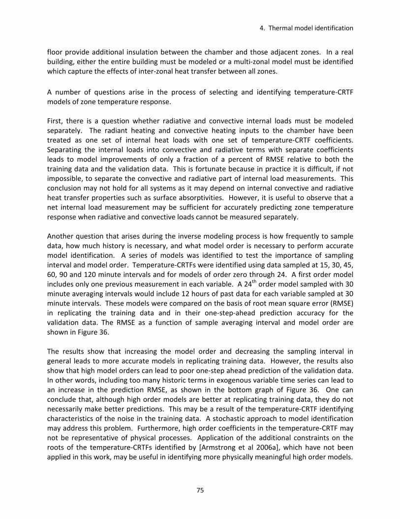
4. Thermal model identification
75
floor provide additional insulation between the chamber and those adjacent zones. In a real
building, either the entire building must be modeled or a multi-zonal model must be identified
which capture the effects of inter-zonal heat transfer between all zones.
A number of questions arise in the process of selecting and identifying temperature-CRTF
models of zone temperature response.
First, there is a question whether radiative and convective internal loads must be modeled
separately. The radiant heating and convective heating inputs to the chamber have been
treated as one set of internal heat loads with one set of temperature-CRTF coefficients.
Separating the internal loads into convective and radiative terms with separate coefficients
leads to model improvements of only a fraction of a percent of RMSE relative to both the
training data and the validation data. This is fortunate because in practice it is difficult, if not
impossible, to separate the convective and radiative part of internal load measurements. This
conclusion may not hold for all systems as it may depend on internal convective and radiative
heat transfer properties such as surface absorptivities. However, it is useful to observe that a
net internal load measurement may be sufficient for accurately predicting zone temperature
response when radiative and convective loads cannot be measured separately.
Another question that arises during the inverse modeling process is how frequently to sample
data, how much history is necessary, and what model order is necessary to perform accurate
model identification. A series of models was identified to test the importance of sampling
interval and model order. Temperature-CRTFs were identified using data sampled at 15, 30, 45,
60, 90 and 120 minute intervals and for models of order zero through 24. A first order model
includes only one previous measurement in each variable. A 24th order model sampled with 30
minute averaging intervals would include 12 hours of past data for each variable sampled at 30
minute intervals. These models were compared on the basis of root mean square error (RMSE)
in replicating the training data and in their one-step-ahead prediction accuracy for the
validation data. The RMSE as a function of sample averaging interval and model order are
shown in Figure 36.
The results show that increasing the model order and decreasing the sampling interval in
general leads to more accurate models in replicating training data. However, the results also
show that high model orders can lead to poor one-step ahead prediction of the validation data.
In other words, including too many historic terms in exogenous variable time series can lead to
an increase in the prediction RMSE, as shown in the bottom graph of Figure 36. One can
conclude that, although high order models are better at replicating training data, they do not
necessarily make better predictions. This may be a result of the temperature-CRTF identifying
characteristics of the noise in the training data. A stochastic approach to model identification
may address this problem. Furthermore, high order coefficients in the temperature-CRTF may
not be representative of physical processes. Application of the additional constraints on the
roots of the temperature-CRTFs identified by [Armstrong et al 2006a], which have not been
applied in this work, may be useful in identifying more physically meaningful high order models.

4. Thermal model identification
76
Based on the relationship between validation data RMSE, model order and sample averaging
interval, it is evident that at least a third or fourth order model is best for achieving accuracy.
High order models may become less accurate, particularly at larger sampling intervals. Using
relatively higher frequency sampling, over 15 to 30 minute intervals, leads to better prediction
RMSEs but with diminishing returns. The local minima in the validation data RMSE surface at 60
minute sampling and third order is likely an artifact of the frequencies used to excite the
chamber, where thermal inputs were varied in a round number of hours.
Changes in the types of internal loads, occupied periods, outdoor climate conditions, and other
characteristics of a building or its use may cause previously identified models to become less
accurate as the building changes or weather and loads deviate from previously observed
conditions. These problems can be mitigated in part by careful selection of model order,
sampling interval and model structure based on validation data RMSE and other goodness of fit
metrics. Another approach is to perform continuous model identification from BAS data over
time. The temperature-CRTF models can be updated continuously based on recent data to
ensure that variations in loads, climate and other characteristics observed are used as new
training data for the building. Continuous refinement will allow the temperature-CRTFs to
improve over time.

4. Thermal model identification
77
0 20 40 60 80 100 120291
292
293
294
295
296
Hour
Temperature (K)
Training temperature input data
AAT
OAT
0 20 40 60 80 100 1200
200
400
600
800
1000
Hour
Power (W)
Training heat input data
Floor heat input
0 20 40 60 80 100 120293
293.5
294
294.5
295
295.5
Hour
Temperature (K)
Predicted ZAT output
ZAT
p-ZAT
0 20 40 60 80 100 120293
293.5
294
294.5
295
295.5
Hour
Temperature (K)
Predicted MRT output
MRT
p-MRT
0 20 40 60 80 100 120293
293.5
294
294.5
295
295.5
Hour
Temperature (K)
Predicted OPT output
RMSE ZAT = 0.05 K, or 0.4 %
RMSE MRT = 0.01 K, or 0.1 %
RMSE OpT = 0.03 K, or 0.2 %
Relative RMSE calculated as a percent of the
range of temperature variation
p = one step ahead predictionOpT
p-OpT
Figure 33 Accuracy of inverse model on training data. The top two graphs show a sample of training data for a
floor heating test. The bottom three graphs show the inverse model's accuracy in predicting zone air
temperature (ZAT), mean radiant temperature (MRT) and operative temperature (OPT). The RMSEs presented
are for the entire training data set, including five sets of training data in addition to that shown

4. Thermal model identification
78
0 20 40 60 80 100294
296
298
300
302
Hour
Temperature (K)
Validation temperature input data
AAT
OAT
0 20 40 60 80 1000
500
1000
Hour
Power (W)
Validation heat input data
0 20 40 60 80 100298
299
300
301
Hour
Temperature (K)
Predicted ZAT output
ZAT
p-ZAT
0 20 40 60 80 100298
299
300
301
hour
Temperature (K)
Predicted MRT output
MRT
p-MRT
0 20 40 60 80 100298
299
300
301
Hour
Temperature (K)
Predicted OPT output
RMSE ZAT = 0.02 K, or 0.7 %
RMSE MRT = 0.02 K, or 1 %
RMSE OpT = 0.01 K, or 0.6 %
Relative RMSE calculated as a percent of the
range of temperature variation
p = one step ahead predicted variableOpT
p-OpT
Radiant floor
heat input
Figure 34 Accuracy of inverse model for floor heating validation data.

4. Thermal model identification
79
0 50 100 150290
295
300
305
Hour
Temperature (K)
Validation temperature input data
AAT
OAT
0 50 100 1500
500
1000
1500
2000
Hour
Power (W)
Validation heat input data
0 50 100 150290
295
300
305
Hour
Temperature (K)
Predicted ZAT output
ZAT
p-ZAT
0 50 100 150290
295
300
305
hour
Temperature (K)
Predicted MRT output
MRT
p-MRT
0 50 100 150290
295
300
305
Hour
Temperature (K)
Predicted OPT output
RMSE ZAT = 0.07 K, or 0.7 %
RMSE MRT = 0.02 K, or 0.3 %
RMSE OpT = 0.04 K, or 0.5 %
Relative RMSE calculated as a percent of the
range of temperature variation
p = one step ahead predicted variable
OpT
p-OpT
Convective
heat input
Figure 35 Accuracy of inverse model for convective heating validation data
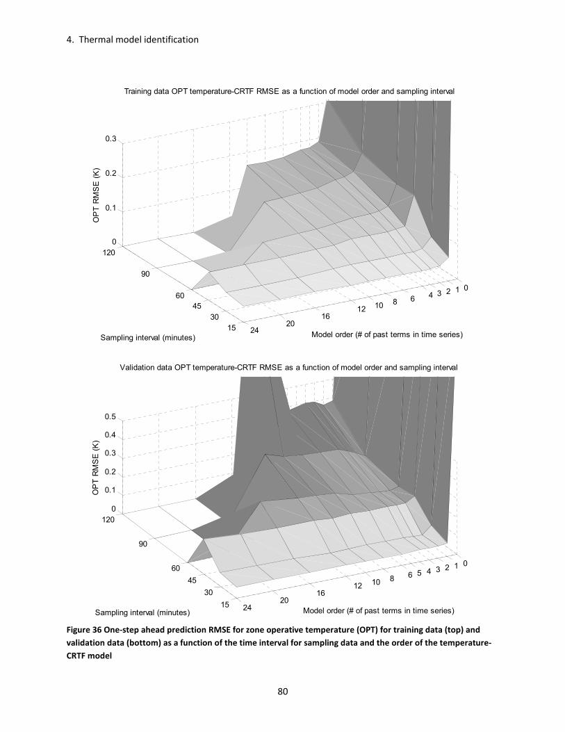
4. Thermal model identification
80
15
30
45
60
90
120
01234568101216
2024
0
0.1
0.2
0.3
0.4
0.5
Model order (# of past terms in time series)
Validation data OPT temperature-CRTF RMSE as a function of model order and sampling interval
Sampling interval (minutes)
OPT RMSE (K)
15
30
45
60
90
120
0123468101216
2024
0
0.1
0.2
0.3
Model order (# of past terms in time series)
Training data OPT temperature-CRTF RMSE as a function of model order and sampling interval
Sampling interval (minutes)
OPT RMSE (K)
Figure 36 One-step ahead prediction RMSE for zone operative temperature (OPT) for training data (top) and
validation data (bottom) as a function of the time interval for sampling data and the order of the temperature-
CRTF model

4. Thermal model identification
81
4.3.2 Application of temperature-CRTFs to a zone with radiant concrete-core cooling
The temperature-CRTF models tested in the previous section were next applied to the test
chamber after installation of a radiant concrete-core floor cooling system. In this case, the
electrical resistance heaters underneath the concrete layers were replaced with a chilled water
loop that provides cooling to the bottom of the concrete. This chilled water loop was supplied
by an air-cooled chiller, created from the split-system air conditioner described in Chapter 3.
This air-cooled chiller system will be described in detail in Chapter 6. The important point is
that the cooling rate to the floor could be measured at the chilled water loop from the chilled
water flow rate and the chilled water supply and return temperature difference. For purposes
of this chapter, the cooling rate to the radiant concrete floor is the only important issue, the
details of providing that cooling will be explained later.
In applying temperature-CRTFs to the chamber cooled with a radiant concrete floor, all modes
of thermal excitation were implemented simultaneously on the chamber, as would be expected
for a real building or zone. These include climate temperature variations due to diurnal cycles,
internal heat loads, and radiant cooling from the floor. Solar loads were not simulated. Light
bulbs were used to simulate internal loads from people, lights and equipment as described in
the section 4.2 and in Appendix B.1. As before, temperature-CRTF models were identified to
predict ZAT, MRT and OPT.
In addition to ZAT, MRT and OPT, a temperature underneath the slab (UST for under-slab
temperature) and the chilled water return water temperature (RWT) were predicted. The UST
is a measure of the pre-cooling of the concrete, and represents an energy state of the concrete-
core TES. A temperature-CRTF identical to equation (13) is used to predict UST, where iT equals
UST. In this case UST is a material temperature and the internal loads, outdoor temperature,
and adjacent zone temperature impact UST through the temperature response of the zone and
furthermore through the conduction transfer function of the concrete floor. As in the heating
tests, the temperature below the floor is neglected, meaning that the chamber below the
concrete floor and chilled water loop is assumed to be adiabatic.
The UST is a useful intermediate temperature for predicting the RWT. As will be explained in
Chapter 5, the RWT is necessary to predict the power consumption of the chiller at future time
steps, which is needed to minimize energy consumption over a 24 hour look-ahead period.
Predicting the RWT could, in theory, be done with a temperature-CRTF using the same variables
used to predict ZAT, MRT, and OPT. Outdoor air temperature, internal loads, and cooling rate
are the only exogenous variables impacting RWT (at a fixed chilled water pump speed).
However, in practice it is impractical and difficult, if not impossible, to predict RWT from these
exogenous variables. In the test chamber, the temperature sensor measuring RWT is installed
in the climate chamber. When the chilled water pump is off, the RWT approaches outdoor
temperature. When the chilled water pump is on, the RWT is determined primarily by the UST
and the cooling rate QC. The chilled water pump speed would also impact RWT, but for
purposes of this research the pump speed has been held constant.

4. Thermal model identification
82
[Olesen et al 2003] and [Koschenz and Dorer 1999] show how thermal RC networks can be
applied to relate chilled water loop temperatures to the temperature of a concrete-core radiant
floor. From an inverse modeling perspective, any thermal RC network that can be represented
in state-space form can be converted to a transfer function representation, as shown in
[Jimenez and Madsen 2008]. Although the order of the thermal RC network relating RWT to
the UST is unknown, it is sufficient to observe that a thermal RC network can be defined
relating cooling rate, UST and RWT. Without a priori knowledge of the order of the system,
transfer function models of increasing order can be identified until RMSE thresholds are met
and any other goodness of fit metrics are satisfied. The following transfer function model was
applied to model RWT:
(18) ∑∑∑===
−+−+−=M
0m
m
M
0m
m
M
1m
m )mt(QCc)mt(USTb)mt(RWTa)t(RWT
RWT is chilled water return temperature, UST is under-slab temperature, QC is the cooling rate,
and M is the number of historic terms in each time series. This is equivalent to stating that the
chilled water temperature forms an Mth order thermal system affected by the cooling rate QC
and the concrete temperature UST.
The training data used for temperature-CRTF model identification of ZAT, MRT, OPT, UST, and
RWT were shown in the previous section in Figure 31. An eighth-order model with data
sampled at 30 minute intervals was used for the ZAT, MRT, OPT and UST temperature-CRTFs
with the same form as equation (13). A second-order model with data averaged over 30
minute intervals was applied for RWT. Averaging for RWT was performed because the transient
response of the chilled water temperature was not of interest, but rather only the near-steady-
state RWT for a given QC and UST. Sampling, rather than averaging, RWT results in very erratic
predictions of RWT at times when the chilled water pump turns on or off. Averaging RWT over
thirty minute intervals and modeling it only when the chilled water pump is on ensures that the
model of RWT relative to UST and QC represents RWT temperature response and a steady
operating condition.
The choice of order for these models will be explained below. Figure 37 shows the one-step-
ahead prediction accuracy of the temperature-CRTF models identified from the training data.
The RMSE for ZAT, MRT, OPT, and UST are within hundredths of a Kelvin, while the RMSE for
RWT is much larger, around 0.8 K.
Validation data, which was not used to identify the temperature-CRTF coefficients, is shown in
Figure 38. A sample of the 24-hour look-ahead accuracy of the temperature-CRTFs for a subset
of the validation data is shown in Figure 39. The 24 hour prediction accuracy is important
because the models will be used to predict zone temperature response 24 hours into the future
in order to optimize chiller control and minimize system power consumption. The validation
data show that the temperature-CRTF models are accurate to within a few tenths of a Kelvin for
ZAT, MRT, OPT, and UST for 24 hour look ahead prediction. Prediction of RWT is noticeably less

4. Thermal model identification
83
accurate, with about a one degree Kelvin RMSE. Figure 40 shows the prediction RMSE for a
sample of the validation data set for predicting further into the future, as far as 96 hours ahead.
Beyond a few days the model predicted temperatures begin to drift away from measured
validation data due to accumulated error.
The model order, eight, and sampling interval, 30-minutes, was selected based on an RMSE
metric as described in the previous section. Figure 41 shows the OPT one-step ahead
prediction RMSE for the training data and for the validation data as a function of model order
and sampling interval. In looking at the one-step-ahead prediction RMSE, fourth order models
or higher with sampling intervals of 15 or 30 minutes are reasonably accurate. However, the
models must predict temperature 24 hours into the future.
Figure 42 shows the total 24-hour-ahead RMSE for the complete validation data set as a
function of model order and sampling interval. The total 24-hour-ahead RMSE is calculated
from the validation data as follows. First, individual 24-hour-ahead RMSE are calculated
beginning with a time series of length N, where N is the model order. These N measurements
of each model input variable form the initial time series history for a 24-hour-ahead prediction
of OPT, UST and RWT. An RMSE can be calculated for the 24 hours of predicted temperatures
relative to the actual measured temperatures. This RMSE is for just one initial set of input
variables. Multiple sets of input variables from the validation data, consisting of N samples of
each input variable, can be used as the initial time series for a 24-hour-ahead prediction. To
calculate the total 24-hour-ahead RMSE for the validation data set, 24-hour-ahead predictions
are made beginning with subsets of validation data from time 1 to N, then 2 to N+1, and so on
through the complete data set. The RMSE for all of the predictions made with all of these initial
data sets are tallied for a complete 24-hour-ahead prediction RMSE for the temperature-CRTF
model based on the validation data set.
The 24-hour-ahead RMSE show in general, as before, that lower RMSE can be achieved with
higher frequency sampling, such as 15 or 30 minute intervals. However, the 24-hour-ahead
RMSE show that somewhat higher model orders, above fifth order, are generally better than
lower model orders at predicting 24 hours ahead. Overall, the best 24-hour-ahead RMSEs are
in the range of 0.4 to 0.5 Kelvin with 15 or 30 minute sampling and a model order of five to
eight. The 24-hour-ahead RMSE is significantly worse than the one-step-ahead RMSEs, which
were closer to one tenth of a Kelvin. A balance must be maintained when selecting model
order to achieve accuracy and reduce complexity and computational time required for
simulation. Fifteen minute sampling would require predictions of 96 temperatures for each
variable over a 24 hour prediction horizon, whereas 30 minute sampling requires half of that.
To strike this balance an eighth order model with 30 minute sampling was elected, allowing for
high accuracy 24 hour ahead prediction while maintaining a reasonable number of predicted
temperatures in the prediction horizon.
A lower order model was applied for RWT prediction. The UST captures the higher order, slow
thermal response of the concrete floor, whereas the transfer function model for RWT captures
the faster temperature response between the UST, cooling rate QC, and RWT. Models of

4. Thermal model identification
84
increasing order for RWT were tested to identify an appropriate temperature response model
for RWT. The RMSE for RWT prediction as a function of model order is shown in Figure 43 for
one-step-ahead prediction of training data and validation data, and 24-hour-ahead prediction
of the validation data. RWT has only been predicted when the chilled water pump is running.
When the pump is off, the RWT is assumed to float back to the outdoor climate temperature
because of the location of the RWT sensor. This has no impact on the thermal response of the
room. Models of order greater than four show no improvement in predicting validation data. A
second order model was elected for predicting RWT from UST and QC.
4.4 Thermal model identification for LLCS
A few observations can be made based on the analysis in this chapter relevant to applying
thermal model identification and temperature-CRTFs to LLCS. First, transfer function models
are well-suited for inverse modeling zone thermal dynamics for LLCS with radiant concrete-core
floors where the thermal mass of the floor is used for energy storage. No a priori knowledge is
necessary about building components or the order of the thermal system. Models of different
system order and with different sampling intervals can be easily identified and compared based
on validation data RMSE. Training data RMSE should not be used to elect model orders,
because increasing RMSE may reflect better modeling of training data noise rather than the
temperature response.
Accurate temperature-CRTF models for the primary temperatures of interest in radiant cooling
can be identified from only a few days of training and validation data. These include air
temperatures, mean radiant temperatures, and operative temperatures. Additional
measurements such as slab temperatures and chilled water loop temperatures can also be
predicted using such models. These temperatures will be important in a 24-hour-ahead
predictive control algorithm, in which chiller power consumption depends on evaporating
temperature, which in turn depends on chilled water temperature.

4. Thermal model identification
85
0 20 40 60 80 100290
292
294
296
298
Hour
Temperature (K)
ZAT
p-ZAT
0 20 40 60 80 100292
294
296
298
Hour
Temperature (K)
MRT
p-MRT
0 20 40 60 80 100292
294
296
298
Hour
Temperature (K)
OpT
p-OpT
0 20 40 60 80 100285
290
295
300
Hour
Temperature (K)
UST
p-UST
0 10 20 30 40275
280
285
290
295
300
Hour
Temperature (K)
Training data RMSEs
RMSE ZAT = 0.05 K
RMSE MRT = 0.02 K
RMSE OpT = 0.04 K
RMSE UFT = 0.03 K
RMSE RWT = 0.79 K
p = one step ahead predicted variable
RWT
p-RWT
Figure 37 Concrete-core radiant floor cooling temperature-CRTF model one-step ahead training data prediction
RMSE for ZAT, MRT, OPT, UST, and RWT

4. Thermal model identification
86
0 20 40 60 80 100 120275
280
285
290
295
300
305
Hour
Temperature (K)
Concrete core cooling validation data temperature outputs
OpT
ZAT
MRT
UST
RWT
0 20 40 60 80 100 120-1500
-1000
-500
0
500
1000
Hour
Heat rate (W)
Concrete-core cooling validation data heat inputs
Internal load QI
Floor cooling QC
0 20 40 60 80 100 120275
280
285
290
295
300
305
Hour
Temperature (K)
Concrete-core cooling validation data temperature inputs
AAT
OAT
Figure 38 Concrete-core radiant floor sample validation data temperature inputs, thermal inputs, and
temperature outputs

4. Thermal model identification
87
0 5 10 15 20 25292
294
296
298
300
Hour
Temperature (K)
ZAT
p-ZAT
0 5 10 15 20 25292
294
296
298
Hour
Temperature (K)
MRT
p-MRT
0 5 10 15 20 25292
294
296
298
300
Hour
Temperature (K)
OpT
p-OpT
0 5 10 15 20 25288
290
292
294
296
Hour
Temperature (K)
UST
p-UST
-1 0 1 2 3 4275
280
285
290
295
Hour
Temperature (K)
Validation data 24 hour look ahead RMSEs:
RMSE ZAT = 0.16 K
RMSE MRT = 0.14 K
RMSE OpT = 0.13 K
RMSE UFT = 0.18 K
RMSE RWT = 1.18 K
p = N step ahead predicted variable
RWT
p-RWT
Figure 39 Concrete-core radiant floor cooling temperature-CRTF model 24-hour-ahead validation data prediction
RMSE for ZAT, MRT, OPT, UST, and RWT
4. Thermal model identification
88
0 20 40 60 80292
294
296
298
300
Hour
Temperature (K)
ZAT
p-ZAT
0 20 40 60 80292
294
296
298
300
Hour
Temperature (K)
MRT
p-MRT
0 20 40 60 80 100292
294
296
298
300
Hour
Temperature (K)
OpT
p-OpT
0 20 40 60 80285
290
295
300
Hour
Temperature (K)
UST
p-UST
-10 0 10 20 30275
280
285
290
295
Hour
Temperature (K)
Validation data RMSEs for 96 hour look ahead:
RMSE ZAT = 0.43 K
RMSE MRT = 0.32 K
RMSE OpT = 0.35 K
RMSE UFT = 0.19 K
RMSE RWT = 1.15 K
p = N step ahead predicted variable
RWT
p-RWT
Figure 40 Concrete-core radiant floor cooling temperature-CRTF model 96-hour-ahead validation data prediction
RMSE for ZAT, MRT, OPT, UST, and RWT

4. Thermal model identification
89
15
30
45
60
234568
1012
1620
24
0
0.05
0.1
Model order (# of past terms in time series)
Concrete-core radiant floor training data RMSE as a
function of sampling interval and temperature-CRTF model order
Sampling interval (minutes)
Temperature (K)
15
30
45
60
234568101216
2024
0
0.05
0.1
0.15
Model order (# of past terms in time series)
Concrete-core radiant floor validation data one-step-ahead RMSE as a
function of sampling interval and temperature-CRTF model order
Sampling interval (minutes)
Temperature (K)
Figure 41 Concrete-core radiant floor OPT temperature-CRTF model one-step-ahead RMSE as a function of
sampling interval and model order for training data (top) and validation data (bottom)

4. Thermal model identification
90
15
30
45
60
23456810
1216
2024
0
0.5
1
1.5
2
Model order (# of past terms in time series)
Concrete core radiant floor validation data 24-hour-ahead RMSE as a
function of sampling interval and temperature-CRTF model order
Sampling interval (minutes)
Temperature (K)
Figure 42 Concrete-core radiant floor OPT temperature-CRTF model 24-hour-ahead RMSE as a function of
sampling interval and model order for validation data
1 2 3 4 5 6 7 80.5
0.6
0.7
0.8
0.9
1
1.1
Model order
Temperature (K)
RWT training data
RMSE vs model order
1 2 3 4 5 6 7 80.5
0.6
0.7
0.8
0.9
1
1.1
Model order
Temperature (K)
RWT 24-hour-ahead validation data
RMSE vs model order
Figure 43 RWT prediction error with 30 minute sampling as a function of transfer function model order,
corresponding to the order of the thermal network between the UST and RWT measurements.

91
Chapter 5 Pre-cooling control optimization The ultimate goal of low-lift cooling is to achieve signficant cooling energy savings by operating
a chiller at low pressure ratios more of the time to meet the daily cooling load. The key control
element enabling low-lift cooling is a predictive pre-cooling control algorithm which optimizes
the operation of a chiller over a 24 hour period by pre-cooling TES. This optimizer must
minimize the power consumption of the chiller while providing enough cooling to maintain
thermal comfort during occupied periods. The predictive control algorithm allows the chiller to
operate at low part-loads more of the time by spreading out cooling load over more hours of
the day and shifting the cooling load to night-time hours, when lower condensing temperatures
are possible. Combined with a radiant cooling system which allows for higher evaporating
temperatures, predictive pre-cooling control enables the low-lift chiller operation at the core of
LLCS.
This Chapter will review previous work on predictive HVAC control algorithms relevant to this
research. It will also describe the development of a chiller control optimization algorithm using
the curve-fit low-lift heat pump model from Chapter 3 and the zone temperature response
models from Chapter 4.
5.1 Predictive control with thermal energy storage and radiant systems
Predictive control of chillers has been used to reduce operating costs and, less frequently,
energy consumption primarily by limiting peak cooling demand and shifting thermal loads. In
some cases, inverse models of building cooling loads have been used simply to calculate the
power consumption for an HVAC system with an assumed demand limiting, energy savings or
cost reduction control strategy. In these cases, simple zone temperature setpoint schedules or
other control schedules are proposed (not determined by an optimization algorithm) which will
reduce energy consumption or operating costs [Braun et al 2001, Braun and Lee 2006, Lee and
Braun 2008].
A more rigorous approach, though one that requires significantly more information, model
complexity, and computational resources is to identify control schedules using an optimization
algorithm. [Braun 1990] takes an approach similar to that developed in this research. An
optimization algorithm is presented that includes: a temperature-CRTF model of zone
temperature response similar to that described in chapter 4; a cooling plant power model as a
function of chilled water loop load, the outdoor wet-bulb temperature, and supply air
temperature difference; and an air handler power consumption model. An optimization is
5. Pre-cooling control optimization
92
performed to minimize the following objective function with respect to zone temperature set
points Tz:
(19) ∑=
×=K
1k
z* ))k(f),k(T(P)k(RJ
vv subject to constraint )k(T)k(T)k(T max,zzmin,z ≤≤
In equation (19), R(k) is an electricity rate at time k and P* is the optimal cooling plant
consumption at time k. The sum is over time k=1 through K where k can be 24 hours into the
uure. P*depends not only on current conditions at time k, but also on zone temperature
setpoints and exogenous variables other times. As a consequence, P* is a function of a vector
of zone temperature setpoints )k(Tz
v and a vector of exogenous variables )k(f
v. )k(fv
includes
solar loads, internal loads and outdoor climate conditions at times k. An optimization over the
vector of temperature setpoints )k(Tz
v is performed to minimize electricity cost (or energy
consumption with R(k) = 1 for all k). The power consumption for HVAC equipment at each time
k is calculated based on cooling loads, computed from a CRTF model, with fixed indoor
temperature setpoints )k(Tz
v.
The cooling loads at a given time k depend on current and past temperature setpoints.
Consequently, calculation of cooling loads, power consumption, and costs at future time steps
requires iteration of the CRTF using zone temperature set point history at each time step. For a
given set point, the power consumption is a non-linear function depending on the operating
state of the HVAC equipment and loads. Furthermore, the power consumption can be
discontinuous as a result of changing operating states in HVAC equipment, such as when a
chiller, pump or fan is on or off. [Braun 1990] applied a direct search method to optimize
equation (19), solving for zone temperature set points that minimize electric costs due to HVAC
power consumption over a 24 hour period.
[Henze et al 1997] develops an optimal pre-cooling control algorithm for ice-storage active TES
under time-of-use (TOU) electricity pricing with a simplified chiller that has only two operating
states. These two chiller operating states are modeled using one electric input ratio (EIR or
1/COP) while the chiller is chilling water and one, separate, lower EIR while the chiller is
generating ice. An optimization is performed to minimize cooling costs by adjusting the time
and duration over which the chiller produces ice for later use, or produces chilled water for
immediate use to meet cooling loads not supplied by discharging the ice-storage. Dynamic
programming is employed for optimization, which can be applied to problems where states are
uniquely defined and do not depend on the path taken to reach a given state, such as the
amount of ice stored in an ice storage system.
In [Henze et al 2004], an optimal chiller control algorithm is developed to minimize cooling
costs for passive and active TES combined under a dynamic utility rate structure. However, the
problem is greatly simplified by assuming, again, a constant chiller COP or EIR for chilled water
and ice-making operation, independent of outdoor temperature and supply air or zone air
temperature. The problem is thus split into two separate optimizations: one in which zone air

5. Pre-cooling control optimization
93
temperature set points are optimized to minimize cooling load (where power consumption is
assumed to be directly proportional to cooling load); and another in which an optimal charging
and discharging schedule for active TES is determined to meet a total daily cooling calculated
from the passive storage optimization. By separating the passive and active TES optimization
problems and treating chiller performance as a constant, the passive TES optimization remains
a linear problem in which zone temperatures are adjusted to minimize cooling load under an
assumed active TES charging and discharging schedule. This allows for the application of a
quasi-Newton optimization method to the passive TES problem, coupled with a dynamic
programming optimization for the active TES problem.
[Snyder and Newell 1990] use a 2R1C building model to find optimal control strategies for
cooling cost minimization through load shifting and demand limiting. However, the problem is
reduced to three variables: the pre-cooling start time; the duration of time the zone is allowed
to float until it reaches maximum allowed temperature; and the thermal mass temperature at
the start of the occupied period.
[Chen 2001, Chen 2002] develop a predictive control algorithm to minimize cost or energy
consumption of a radiant floor heating system. Similar to [Henze et al 2003], the efficiency of
the heating plant is not weather dependent or dependent on past heating rates. As a result,
the optimization problem remains linear in thermal loads and temperature response.
[Wang and Ma 2008] provides an overview of supervisory and optimal control methods for
HVAC systems. It includes a review of optimization methods employed for supervisory or
predictive HVAC control such as direct search, sequential quadratic, conjugate gradient,
simulated annealing, genetic algorithm, and others.
Drawing from this past research, a framework for a pre-cooling control optimization will be
developed that determines on optimal chiller control schedule for each hour, 24 hours-ahead,
that pre-cools a concrete-core radiant floor/TES system to maintain thermal comfort later in
the day.
5.2 LLCS pre-cooling control objective function
The goal of the LLCS control is to minimize cooling energy consumption (or cost) of the LLCS
over a 24-hour period by controlling cooling rate in a near optimal way. This near-optimal
control function incorporates the performance map model of chiller power consumption from
chapter 3, the temperature-CRTF models of the zone being controlled from chapter 4, and
thermal comfort conditions desired in the zone. The optimization function can be described
mathematically as follows:
(20) ( )∑=
ω +ϕ+=24
1t
tttt PENEVTPENOPTPrJminarg

5. Pre-cooling control optimization
94
In equation (20), the objective function J is the sum over 24 hours of the cooling system power
consumption, a penalty for operative temperatures outside of the comfort range, and a penalty
for evaporating temperatures below a low temperature threshold. The variables are as follows:
• rt is a weighting factor for system power consumption. rt can be set to one for an
energy consumption minimization or to a TOU pricing schedule for cost minimization
(not including demand charges),
• Pt is the energy consumption of the cooling system over the hour t,
• � is a weighting factor for the operative temperature penalty,
• PENOPTt is a penalty function for operative temperatures outside of a desired comfort
range at time t,
• PENEVTt is a penalty function for evaporating temperatures below a low temperature
threshold, which has been included to prevent control predictions that would cause the
chiller to freeze.
The power consumption Pt is a non-linear function derived from the heat pump curve-fit models
in Chapter 3, given by the following equation:
(21) )),EVT,OAT(f,,EVT,OAT(PPP ttttttchiller_cooled_air,tchwpump,tt ωω+=
• Pt,chw_pump is the energy consumption of the chilled water pump over the hour t. The
chilled water pump is operated at constant speed while the chiller is on. Thus, its power
consumption is either zero if the chiller is off or a constant while running.
• Pt,air_cooled_chiller is a curve-fit model of the air-cooled chiller power as a function of
outdoor air temperature OAT, evaporation temperature EVT, compressor speed ω , and
fan speed f at hour t.
The curve fit model for the air-cooled chiller is derived in the same way as the heat pump
model from Chapter 2, except that the zone air temperature in equation (10) is replaced with
the refrigerant evaporating temperature EVT as an independent variable. This curve-fit model
is shown in equation (22) with the independent variables evaporating temperature EVT,
outdoor air temperature OAT, compressor speed ω, and fan speed f. The RMSEs for this curve-
fit model with evaporating temperature as an independent variable are 5.8 percent or 29
Watts, similar to the accuracies found in chapter 3 for the air-cooled heat pump.
(22)
t2524232
2221
202
192
18
217
216
215
214
313
312
311
10982
72
62
5
4321
chiller_cooled_air,t
fCOATfCEVTfCfCfC
OATEVTCOATCEVTC
OATCEVTOATCEVTCOATEVTC
COATCEVTC
OATCEVTCOATEVTCCOATCEVTC
COATCEVTCC
P
ω+⋅+⋅++
+ω⋅+ω+ω
+ω++ω+
+ω++
+ω+ω+⋅+ω++
+ω+++
=

5. Pre-cooling control optimization
95
Similar models with the same form as equation (22) have been identified for cooling capacity
Qt,air_cooled_chiller and electric input ratio EIRt,air_cooled_chiller as a function of EVT, OAT, ω, and f. The
RMSE for those models are 1.5 percent or 31 Watts and 4.4 percent or 0.01 kWe /kWth
respectively. The coefficients for each of these curve-fit models are shown in Appendix A.4.
Only two of these three curves, the cooling Qt,air_cooled_chiller and the power consumption of the
chiller Pt,air_cooled_chiller are used in the pre-cooling optimization. The cooling rate Qt,air_cooled_chiller
at each time step is need to compute zone temperature response, shown below, where QC(t)
equals Qt,air_cooled_chiller. The power consumption, Pt,air_cooled_chiller, is needed to compute the
power at time t, Pt, in equations (20) and (21).
The fan speed variable can be eliminated from equation (22) by choosing the optimal fan speed
for a given EVT, OAT, and ω. By taking a partial derivative of the EIRt,air_cooled_chiller curve with
respect to f, the optimal fan speed fopt is seen to be as follows:
(23) ( ) 2225242321opt C2/COATCEVTCCf ω+++=
The presence of EVT in equation (22) requires that evaporating temperature be predicted,
based on engineering calculations or data-driven models, from the chilled water supply or
return temperatures and the chilled water flow rate. For a fixed water flow rate, EVT can be
related directly to one water temperature if the chiller is operated with constant superheat
control for a given compressor speed. The chilled water return temperature (RWT) will be used
to predict EVT. Under steady state operation, the superheated refrigerant vapor temperature
at the evaporator outlet approaches RWT and a closed loop superheat control algorithm relates
evaporator outlet temperature to evaporating temperature EVT as a constant temperature
difference for a given compressor speed. This will be discussed in more detail in chapter 6.
Thus, EVT can be estimated from RWT. A model for RWT was developed in chapter 4 as a
function of cooling rate QC history, RWT history, and under-slab temperature (UST) history:
(24) ∑∑∑===
−+−+−=N
0n
n
N
0n
n
N
1n
n )nt(QCc)nt(USTb)nt(RWTa)t(RWT
As explained in chapter 4, UST is calculated from a temperature CRTF model of the form:
(25) ∑∑∑∑∑=====
−+−+−+−+−=N
0n
n
N
0n
n
N
0n
n
N
0n
n
N
1n
n )nt(QCe)nt(QId)nt(AATc)nt(OATb)nt(USTa)t(UST
In equation (25), OAT is the outdoor (climate chamber) air temperature, AAT is an adjacent
zone temperature, QI is the internal heat load, and QC is the cooling rate. At a given time, the
evaporating temperature EVT can be calculated from the current return water temperature and
the chiller power consumption and cooling rate can be calculated from equation (22) and a
similar equation for Qt,air_cooled_chiller. At a future time t, UST and RWT must be predicted from
previous (both measured and predicted from the current time to future time t) cooling rates,
forecast outdoor temperature, adjacent zone temperature, and internal loads up to time t.

5. Pre-cooling control optimization
96
The second term in equation (20) accounts for the operative temperature of the zone. Without
this term the minimal power consumption would equal zero at all times. The operative
temperature penalty function is given by the following equation:
(26)
+≥−−
−<<+
+≤−+
=
5.0OPTOPT))5.0OPT(OPT(
5.0OPTOPT5.0OPT0
5.0OPTOPT)OPT)5.0OPT((
PENOPT
maxt2
maxt
maxtmin
mint2
tmin
t
OPT is calculated from a temperature-CRTF identified in chapter 4 as follows:
(27) ∑∑∑∑∑=====
−+−+−+−+−=N
0n
n
N
0n
n
N
0n
n
N
0n
n
N
1n
n )nt(QCe)nt(QId)nt(AATc)nt(OATb)nt(OPTa)t(OPT
The weight � in the operative temperature penalty function equates temperature excursions
outside the comfort range to power consumption. A good choice of � is one for which the
amount of energy consumption added to the penalty function for a operative temperature
excursion just outside the comfort bounds is greater than the energy consumption required to
run the chiller to prevent that excursion. For example, under most conditions the air-cooled
chiller consumes less than 180 to 220 Watts at the slowest compressor speed. A � of 300
Watts/K2 results in a lower cost function with the compressor on than off under most
conditions if the operative temperature begins to drift more than 0.25 to 0.5 K outside of the
comfort region. The operative temperature range is chosen to be roughly 19 to 25 Celsius
based on the summer (or 0.5 clo) operative temperature comfort range presented in [ASHRAE
2007a]. A graph of the operative temperature penalty term �PENOPTt is shown in Figure 44.

5. Pre-cooling control optimization
97
16 18 20 22 24 26 280
500
1000
1500
2000
Operative temperature (K)
Power equivalent penalty (W)
Operative temperature power penalty
Figure 44 Operative temperature penalty term ����PENOPT
The last term in the objective function, PENEVTt is a constraint on the evaporating temperature
of the refrigerant EVT. EVT is constrained to prevent freezing of the chiller, or more precisely to
prevent predictions of infeasible cooling rates at future time steps that would cause the chiller
to freeze. The constraint on EVT was chosen conservatively to prevent EVT below one degree
Celsius, with an infinite penalty for evaporating temperatures below the threshold (replaced by
a very high penalty value in computer code). This choice was made to prevent any freezing,
even if just locally on a heat exchanger surface, on the water-side of the chiller. The resulting
evaporating temperature penalty function is as follows:
(28)
≤
>=
1)RWT(EVTINF
1)RWT(EVT0PENEVT
t
t
t
An alternative approach would be to apply the evaporating temperature constraint as a
limitation on system operation. Penalizing the evaporating temperature in the objective
function was convenient, because it eliminated the need to include additional constraints to the
chiller curve-fit model. Furthermore, the OPT penalty function could have been incorporated as
a constraint on operative temperatures. However, this approach does not allow for a simple
tradeoff between comfortable temperatures and power consumption, which is useful for
allowing some overheating as the optimization searches for the best chiller control schedule. If
the OPT penalty was included as a constraint on OPT, or similarly if the weight � for PENOPT
was infinite, additional discontinuities in the search space would be introduced which would
create many deep local minima at compressor speed schedules for which thermal comfort
criteria was met.

5. Pre-cooling control optimization
98
5.3 LLCS pre-cooling control optimization
In the previous section, an objective function was defined for the pre-cooling control algorithm
which contains penalties for power consumption of the cooling system, operative temperatures
outside of a comfort region, and low evaporating temperatures. The goal of this section is
describe how the objective function, equation (20) is minimized to optimize the chiller control
over a 24 hour look ahead schedule.
Each hourly cost component of the objective function must be evaluated sequentially from
hour one to 24. This is a result of the fact that Pt, PENOPTt, and PENEVTt all depend on past
values of both the independent and dependent variables. As the simulation moves into the
future, the choice of compressor speed at simulation time tsim depends on previous values of
compressor speeds at times t<tsim and will affect the choice of future compressor speeds at
times t>tsi,. A given compressor speed at time step tsim will determine QC, and along with
current outdoor air temperature OAT, adjacent zone air temperature AAT, and internal loads QI
and their histories determine OPT, UST, RWT, and EVT at the next time step in the simulation.
The power consumption and cooling rate of the chiller are non-linear functions of OAT, EVT,
and ω (with fan speed fopt determined by these three variables). Consequently, the power
consumption of the chiller at the current simulation time depends non-linearly both on the
choice of compressor speed at the current time tsim and previous choices of compressor speeds
which determine the concrete slab temperature UST and EVT at tsim. Furthermore, when the
compressor speed is zero the cooling system is off and the power consumption and cooling rate
become zero discontinuously, because the compressor cannot run at arbitrary speeds down to
zero Hz.
As a result of these discontinuities and non-linearities in the objective function, an optimization
method suitable for non-linear objective functions must be used. A simple form of direct
search, called a pattern search was selected as an optimization method [Torczon 1997, Lewis et
al 1999, Lewis et al 2000, Audit and Dennis 2003]. The pattern search seeks optimal
compressor speeds for every hour t in a 24-hour-ahead schedule of chiller operation. Pattern
search is essentially a grid search on the independent variable, where an initial guess is made
and points in a grid around that guess are evaluated for a more optimal solution. Pattern
search continues to search the grid until no more optimal solutions can be found, at which
point it reduces the size of the grid and searches more locally around the optimal solution
identified by the larger grid. What follow is a more detailed explanation of the pattern search
algorithm employed in the experimental LLCS concrete-core radiant floor installation described
in chapter 6.
As previously mentioned, the pattern search is essentially a grid search, where the grid size can
change when more optimal solutions cannot be found using the current grid. Pattern search
begins at an initial point in a grid that spans the entire search space. For this research, the
search space is a 24-dimenstional space, where each dimension represents a possible chiller

5. Pre-cooling control optimization
99
compressor speed at each hour of a 24-hour-ahead schedule. The compressor speed at each
hour can take the values of 0 Hz, or off, and anywhere between 19 Hz and 95 Hz. Some speeds
will cause infinite penalties if the temperature-CRTF models determine that they will cause the
chiller to freeze.
Beginning with a guess at an initial point in the 24-dimensional grid, pattern search evaluates
the objective function at all of the grid points surrounding the initial guess. This is called a poll.
All of these grid points are compared to identify the most optimal solution relative to each
other and to the initial guess. If a more optimal grid point is identified, the pattern search
continues by polling a grid around the new optimal solution. The grid size is increased, up to
maximum selected by the user, each time a more optimal point in the grid is identified. If a
more optimal grid point is not found, the pattern search continues around the current point
with a smaller grid size, down to a minimum grid size. The pattern search continues searching
the grid until no more optimal points can be found at the smallest grid size. For the pattern
search implemented here, the starting grid size is 4 Hz, which is the difference between
compressor speeds in each dimension of the 24-dimensional grid. The maximum grid size is
four Hz and the minimum grid size is one Hz.
An optional step in a pattern search is the execution of a secondary optimization on the current
grid point each time a new optimal solution is found around that point. Instead of immediately
polling the grid around the new optimal solution, a search of the other dimensions of the grid
(not the dimension in which a new optimal point has been found) is conducted to identify
whether an even more optimal solution can be found. This allows the pattern search to
perform faster, by moving in more than one-dimension of the grid at each iteration.
To summarize, pattern search is simply a grid search where the size of the grid changes. In its
most basic implementation, pattern search starts with an initial guess in the grid, evaluates the
objective function at all the adjacent grid points, proceeds to the most optimal point in the grid
around the initial guess, then uses that new optimal point as the basis of a new pattern search.
Adjusting the grid size and performing a secondary search on each grid point are simply
methods for avoiding local minima and decreasing pattern search execution time.
A complete explanation of the pattern search algorithm is included Matlab’s Global
Optimization Toolbox: User’s Guide [2010] and more information can be found in [Torczon
1997, Lewis et al 1999, Lewis et al 2000, Audit and Dennis 2003]. A flow chart of the pattern
search implemented for the LLCS predictive pre-cooling control optimization is shown in Figure
46. This chart shows the process from the input, an initial guess of 24 compressor speeds at
each hour of a 24-hour-ahead schedule, to the output, an optimal schedule of 24 compressor
speeds. Each time the algorithm calls for the calculation of the objective function J in equation
(20), equations (21) through (28) are applied to calculate the Pt, QC, OPT, UST, and RWT at each
time step, from which the total value of J can be calculated by summing over all 24 future
hours. Because a 30 minute temperature-CRTF model was elected for OPT, UST, and RWT in
chapter 4, two values for each of these variables are calculated at every hour.
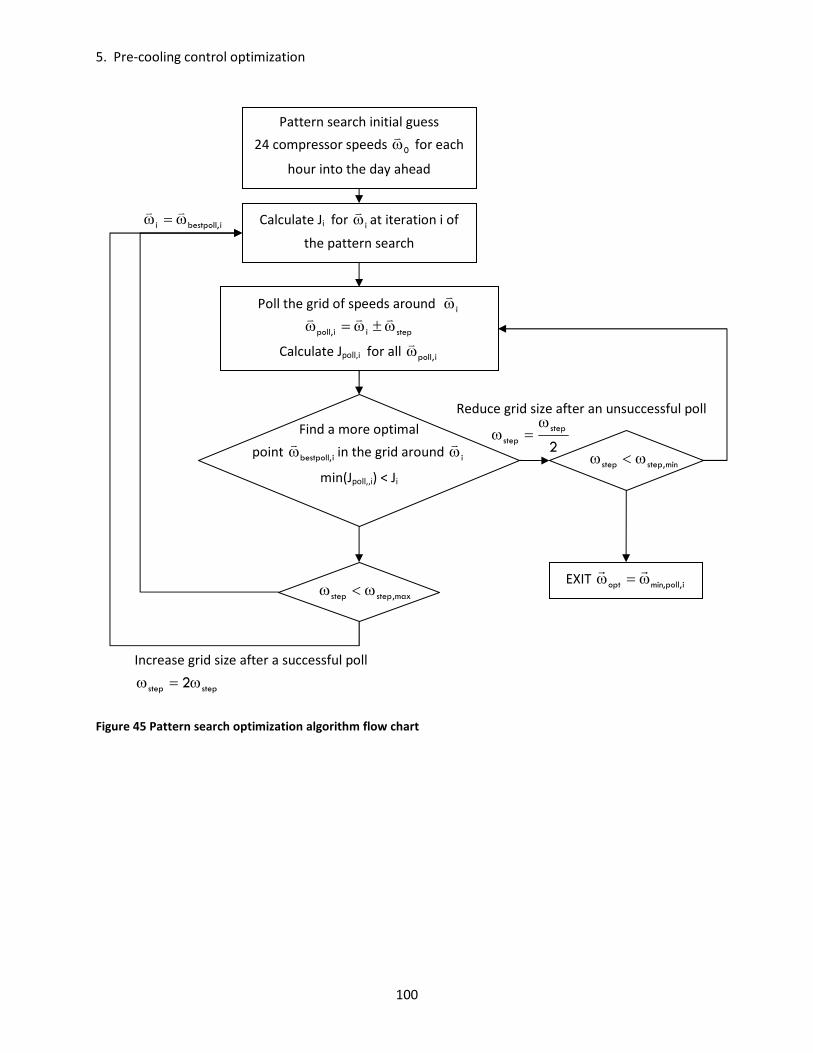
5. Pre-cooling control optimization
100
Pattern search initial guess
24 compressor speeds 0ωv
for each
hour into the day ahead
Calculate Ji for iωv
at iteration i of
the pattern search
Poll the grid of speeds around iωv
stepii,poll ω±ω=ωvvv
Calculate Jpoll,i for all i,pollωv
Find a more optimal
point i,bestpollωv
in the grid around iωv
min(Jpoll,,i) < Ji
2
step
step
ω=ω
min,stepstep ω<ω
max,stepstep ω<ω
EXIT i,pollmin,opt ω=ωrr
Reduce grid size after an unsuccessful poll
Increase grid size after a successful poll
stepstep 2ω=ω
i,bestpolli ω=ωvv
Figure 45 Pattern search optimization algorithm flow chart

5. Pre-cooling control optimization
101
The pattern search algorithm is employed at every hour to calculate a new set of optimal
compressor speeds for the next 24 hours. This allows for the use of updated forecasts of
outdoor air temperature OAT, adjacent zone air temperature AAT, and internal loads QI at each
hour. Only the first compressor speed computed by the pattern search is used to set the
compressor speed for the following hour. The remaining 23 compressor speeds are used as an
initial guess for the new pattern search at the next hour, with the 24th speed equal to zero. A
new pattern search is then performed at the next hour to identify a new optimal set of 24 hour
compressor speeds for the following 24 hours. This process is outlined in Figure 46. [Henze et
al 2003] refers to this approach as closed loop optimization, where feedback from the previous
time step (hour) and updated forecasts are used to determine a new optimal control schedule.
An alternative approach is consecutive time block optimization [Henze et al 2004], in which
compressor speeds are predicted once at the beginning of a 24 hour time block. This approach
is identical to closed loop optimization only in the case where model predictions and exogenous
variable forecasts are perfect. In this research, although exogenous variables are being
controlled, they are not being controlled perfectly and a closed loop optimization is more
effective than consecutive time block optimization.
A sample result of the pattern search algorithm is shown in Figure 47. A predicted optimal
compressor speed schedule, with a compressor speed for each of 24 hours into the future, is
shown at the top schedule. For this schedule, the operative temperature OPT, underslab
temperature UST, return water temperature RWT, evaporating temperature EVT, cooling rate
QC, and chiller power consumption P are predicted for each half hour of the 24 hours ahead. At
Pattern search initial guess
ωv
Pattern search algorithm
0i ω=ωvv
Begin predictive control with
{ }0241n,00 =ω=ω →=
v
Operate compressor at
1,optω=ω for one hour
{ }241n,optopt →=ω=ωv
{ }0,242n,opti →=ω=ωv
24 hour-ahead forecasts
of OAT, AAT, QI
Figure 46 Closed loop optimization of compressor speed

5. Pre-cooling control optimization
102
the top right of Figure 47, the predicted OPT, UST, RWT, EVT for the 24 hour ahead period are
shown along with the outdoor temperature OAT and the comfort constraint OPTmax and OPTmin.
The chiller power at each time step and the cumulative energy consumption over the 24 hour
period is shown at the bottom. The dependent variables are predicted at half hour increments
because the temperature-CRTF models make predictions in half hour increments. For the hour
following this optimization, the chiller is operated at the first predicted optimal compressor
speed, which is 0 Hz, or off, in the case below.
The example below demonstrates certain important aspects of low-lift predictive pre-cooling
control. First, the best time to perform most of the cooling is over night and during the early
morning hours. The outdoor air temperature OAT is low and the chiller can run more efficiently.
Second, the chiller runs at relatively low speed (19 Hz is its minimum) most of the time, and
thus at low pressure ratios. Third, near the beginning of the scheduled operation of the
compressor, at hours six, seven and eight, the compressor is scheduled to cycle on for an hour,
then off for an hour, and then turn back on. The optimization has determined that it is more
efficient not to run the compressor continuously for those three hours because it decrease UST,
RWT, and most importantly EVT causing the chiller to run less efficiently at higher evaporating
temperatures. Lastly, at the end of the scheduled pre-cooling the compressor turns off for an
hour and then back on. This is the result of the evaporating temperature EVT approaching the
low temperature threshold of one degree Celsius. The compressor is not allowed to run at hour
16 to prevent the chiller from freezing. This freezing constraint can be avoided by improving
the design of the concrete-core radiant floor so that the difference between chilled water
temperatures RWT and the concrete-core temperature UST is less.
The optimization is not especially sensitive to small changes in the compressor speed setpoint
schedule. Adjusting the compressor speed by one Hz at a given hour will only marginally
change the total energy consumption, by perhaps 10 to 50 Watt-hours or less than one percent
of daily energy consumption. On the other hand, turning the compressor off for an hour or
running it significantly faster may lead to a difference in energy consumption of a few hundred
Watt-hours in the range of five to ten percent of daily energy consumption
Other optimization methods may be applicable to the LLCS predictive pre-cooling control
problem and further research is necessary to evaluate the best optimization method for LLCS.
For this research, however, pattern search was found to identify near-optimal solutions within a
few minutes, whereas applying genetic algorithms or simulated annealing required hours of
optimization time and did not always converge to a solution. Careful tuning and a
comprehensive comparison of alternative optimization methods to the LLCS pre-cooling
optimization problem may still yield a more appropriate optimization method than the pattern
search employed here.

5. Pre-cooling control optimization
103
0 6 12 18 240
10
20
30
40
hour
Temperature (C)
0 6 12 18 240
500
1000
1500
2000
Hour
Cumuluative energy
consumption (Wh)
0 6 12 18 240
50
100
150
200
250
Hour
Chiller Power (W)
0 6 12 18 240
5
10
15
20
25
30
hour
Compressor speed (Hz)
OPT
OAT
RWT
UST
EVT
OPTmax
OPTmin
Total energy
consumption over
24 hours = 1921 Wh
Figure 47 Sample pattern search results, including predicted OPT, RWT, and UST over a 24 hour look ahead (top
left), cumulative energy consumption (top right), chiller power consumption at each half hour (bottom left), and
predicted optimal compressor speed at each hour (bottom right)

104
Chapter 6 Low lift cooling experimental assessment The primary objective of this thesis is to develop and experimentally test the performance of
predictive pre-cooling control for low-lift cooling systems. To achieve this, a radiant concrete-
core floor cooling system served by an air-cooled chiller was installed in the test chamber
described in chapter 4. A concrete-core system was elected as the TES component of the LLCS
because, in theory, it has high thermal storage efficiency. Furthermore, less research has been
done on the coupling concrete- core system pre-cooling control and coupling with a predictive
control of a chiller. Radiant concrete-core systems are also known as thermo-active building
systems or TABS.
This chapter will describe the construction and performance of a concrete-core radiant floor
cooling system (or TABS) in a near full scale experimental installation. This will include the
design and installation of the system, instrumentation for measuring its performance, controls
implemented for both local and supervisory predictive pre-cooling control, and installation of a
split-system air conditioner (SSAC) used as a baseline. These two systems were tested subject
to the same thermal inputs, a typical summer week for Atlanta, Georgia and typical standard
efficiency internal loads. The energy and thermal comfort performance of the LLCS system will
be compared to that of the SSAC under conventional thermostatic control.
6.1 Description of experimental systems
In order to test the performance of the LLCS, a near full-scale demonstration was constructed
of a single-zone room served by an air-cooled chiller that provides chilled water to to a radiant
concrete-core floor. This will be called the LLCS test chamber. The methods described in
chapters 2 through 5 were applied to this system for predictive pre-cooling of the concrete
floor. The LLCS test chamber allows for testing of an LLCS subject to different climates and
under different loads. The system also enables comparison of LLCS energy consumption and
thermal performance to a conventional, variable speed high-efficiency split-system air
conditioner (SSAC) with a SEER rating of 16 Btu/Wh. The following sections will describe the
cooling systems, the systems used to experimentally simulate climate and internal thermal
loads, and the instrumentation installed for performance measurement and control.
6.1.1 Low-lift cooling system
The primary mechanical system for the demonstration LLCS is a variable capacity air-cooled
chiller serving a concrete radiant floor. A Mitsubishi MUZ-A09NA-1 air conditioner/heat pump

6. Low lift cooling experimental assessment
105
outdoor unit, the same model characterized in chapter 3, was used to create the variable
capacity chiller. The outdoor unit contains the compressor, condenser, condenser fan,
expansion valve and electronics for the system. To chill water instead of cooling air, a separate
refrigerant loop was created through a brazed plate heat exchanger (BPHX) between the stop
valve exiting the expansion valve and the stop valve entering the compressor on the outdoor
unit. The BPHX acts as a counter flow heat exchanger between the refrigerant loop and a water
loop which serves the radiant floor. A schematic of the variable capacity chiller is shown in
Figure 48 and a schematic of the water loop serving the concrete radiant floor is shown in Figure
49. Detailed information about the make and model of the equipment are shown in Appendix
C.1.
Control over the compressor speed, condenser fan speed, and electronic expansion valve
position was achieved through a manufacturer’s interface to the Mitsubishi electronic control
board. Serial commands from a desktop computer to this interface could adjust the
compressor speed from 19 to 115 Hz, the condenser fan speed from 300 to 1200 RPM, and the
expansion valve position from fully closed to fully open. The compressor speed and fan speed
commands adjust the output from two separate inverters. The expansion valve commands
control a stepper motor which moves the electronic expansion valve.

6. Low lift cooling experimental assessment
106
BPHX
WATER PUMP
TEST CHAMBER CLIMATE CHAMBER
TO CHILLER
FROM CHILLER
FILTER
EXPANSION TANK
12’
17’
RADIANT
MANIFOLD
RADIANT FLOOR
CONDENSER
ELECTRONIC
EXPANSION VALVE
COMPRESSOR
BPHX
TO RADIANT
FLOOR
FROM RADIANT
FLOOR
FROM INDOOR
UNIT (CLOSED)
TO INDOOR
UNIT (CLOSED)
TEST CHAMBER CLIMATE CHAMBER
LEV
Figure 48 Low-lift cooling system: variable capacity chiller
Figure 49 Low-lift cooling system: radiant floor water loop

6. Low lift cooling experimental assessment
107
Control over the expansion valve was customized for operation of the system as a chiller. A
temperature difference provided by temperature sensors on the refrigerant inlet and outlet
ports of the BPHX provided a measure of the refrigerant superheat across the BPHX evaporator.
Constant superheat control could be implemented using this temperature difference. The
superheat setpoint is a function of compressor speed, as shown in Figure 50. The superheat-
compressor speed relationship was determined by observing the minimally stable superheat
over a range of compressor speeds. The compressor speed was limited to less than 50 Hz
under LLCS operation because higher speeds caused the BPHX temperatures to approach
freezing rapidly. This limitation did not constrain LLCS chiller operation because the predictive
control algorithm called for speeds below 50 Hz all of the time for the loads and climates
tested, which will be described later. A proportional-integral-derivative (PID) control law was
implemented for the electronic expansion valve to maintain constant superheat at a given
compressor speed.
The radiant floor water loops in the schematic in Figure 49 lie embedded in Warmboard radiant
subflooring underneath three layers of concrete pavers, as described in chapter 4. There are six
parallel water loops each made of one half inch polyethylene (PEX) pipe. These six parallel
loops were designed to minimize the pressure drop through the radiant floor and reduce
pumping power. The pipes are spaced 12 inches apart center to center, with the aluminum
surface of the Warmboard enhancing heat transfer between the pipe and bottom layer of the
concrete layers. In a typical installation, the radiant loop piping would be more closely spaced
(four to six inches) and embedded directly in poured concrete. However, pouring concrete was
impractical in the lab setting in which the demonstration was built. Embedding pipe in
Warmboard with an aluminum surface to enhance heat transfer to the concrete layer was a
necessary compromise to mimic a poured concrete-core radiant floor.
The chilled water pump serving the radiant floor loops was operated at a constant speed of 2.1
gallons per minute (GPM). Ideally, an LLCS would include a variable speed chilled water pump
which can be optimized to provide the highest COP under a given set of conditions. In this case,
20 25 30 35 40 45 503
4
5
6
7
8
9
Compressor speed (Hz)
Superheat (K)
Figure 50 Superheat control set point vs compressor speed

6. Low lift cooling experimental assessment
108
because the chiller performance was measured as a function of compressor speed, condenser
fan speed, outdoor temperature and evaporating temperature it was necessary to provide a
simple relationship between water loop operation and the chiller evaporating temperature.
The simplest method to achieve this was to operate the chilled water pump at a constant
speed. This did not penalize chiller performance much because, even at the full speed of 2.1
GPM the specific pump power was very low, about 9 Watts per GPM, due to the low pressure
drop across the radiant floor loops and the efficiency of the pump. The superheat set point as a
function of compressor speed could be determined for fixed chilled water pump speed, and
correspondingly the evaporating temperature EVT could be related directly to a return water
temperature RWT.
Future research could test variable speed chilled water pumping by mapping the performance
of the chiller, in terms of power, cooling capacity, and COP, as a function of chilled water pump
speed in addition to compressor speed, condenser fan speed, outdoor air temperature, and
evaporating temperature. More precisely the evaporating temperature could be replaced by
two variables, chilled water pump speed/flowrate and return water temperature, both of which
will affect evaporating temperature and subsequent chiller performance. This directly parallels
the condenser side where outdoor air temperature and condenser fan speed relate to
refrigerant condensing temperature. With this revised model of chiller performance the
compressor speed, condenser fan speed, and chilled water pump speed can all be adjusted to
optimize the performance of the chiller under 24-hour-ahead pre-cooling control [Armstrong et
al 2009b].
Alternatively, a relationship between the chilled water distribution system operation and
control and the evaporating temperature could be determined separately for any system
served by the chiller. In that case, the chiller performance curves as a function of evaporating
temperature could still be used with the predictive control algorithm, but a separate water
distribution system model would be necessary to relate UST with the evaporating temperature
of the chiller.
Although the chiller was constructed from a heat pump outdoor unit of the same model,
Mitsubishi MUZ-A09NA-1, as that tested in chapter 3, it had slightly different performance
curves. The new outdoor unit did not exhibit the exact same relationships between cooling
rate QC, power consumption P, and electric input ratio EIR (or 1/COP) as the MUZ-A09NA-1
described in chapter 3. Modifications to the system for operation as an air-cooled chiller
caused degradation in system performance. For a given set of conditions, the chiller was
observed on average to achieve only 78 percent of the cooling rate predicted by the curve-fit
model and measured previously while operated with an air-heated evaporator. With this
reduced capacity, the power consumption also dropped to an average 89 percent of the model-
predicted power consumption, and correspondingly the EIR increased, leading to a COP that
was only 82 percent of the original outdoor unit’s COP.
The reasons for this loss in performance are not entirely understood. Some differences in
performance between the two outdoor units was expected because they contain different

6. Low lift cooling experimental assessment
109
parts, although they are of the same make and model. However, the magnitude of the
differences in performance was larger than expected. Expectations were that the performance
of the outdoor unit combined with the BPHX would be higher than that with the air-heated
evaporator. The refrigerant-to-water counterflow BPHX should, in theory, be more effective
than the cross-flow refrigerant-to-air finned tube heat exchanger. On the other hand, the
finned tube heat exchanger has been designed by the manufacturer specifically for use with the
MUZ-A09NA, whereas the BPHX has been generically matched to the outdoor unit’s capacity.
This may explain some of the difference in performance.
The observations of reduced capacity and efficiency may also relate to sub-optimal transient
performance of the system. The performance models described in chapter 3 refer to the steady
state power, cooling capacity, and 1/COP of the system, which is typically not reached until the
system has been operating for over an hour. Furthermore, the curve-fit models of performance
apply to the system when it is controlled for, approximately, a two to three Kelvin superheat
across the air-heated evaporator for all compressor speeds. Under operation of the system
with the BPHX a superheat of three Kelvin was only achievable at the slowest speeds.
Superheat temperatures as high as six Kelvin were the lowest achievable for the highest
compressor speeds. These higher superheats at high compressor speeds may cause some of
the loss in capacity.
Data from which these observations were made are shown in Figure 51. Some of the spread in
the data is a result of measurements being taken under transient operation and the chiller not
reaching steady state. The cooling rate and power consumption predicted by the chiller model,
equation (22), were scaled based on these results to ensure accurate prediction of cooling rate
and power consumption for use in the temperature-CRTF models and the pre-cooling control
optimization. It may be possible to get better performance out of the air-cooled chiller through
better design of the BPHX and better expansion valve control. In theory, performance of the
system with the BPHX should be at least as good as that of the air-heated evaporator.
Images of the chiller constructed from the modified Mitsubishi MUZ-A09NA-1 are shown in
Figures 52-55. Figure 52 shows the condenser and condenser fan, housed in the original
outdoor unit, along with the compressor and electronics which have been removed and heavily
insulated at the bottom of the picture. The pre-insulation refrigerant and chilled water piping,
including the branches that lead separately to the BPHX or to the air-side evaporator, are
shown in Figure 53. The BPHX is located on the far left of the image. The chilled water flow
meter and pump can be seen near the center and bottom of the image. Figure 54 shows the
radiant floor system including the radiant floor manifold, the Warmboard subfloor, and the PEX
pipe embedded in the Warmboard acting as the radiant floor chilled water loops. The six loops
were balanced for equal flow using balancing valves on the radiant system manifold. The air-
side evaporator served under conventional split-system air conditioner operation, described in
the next section, is also shown. Figure 55 shows the completed LLCS test chamber with the
concrete pavers installed.
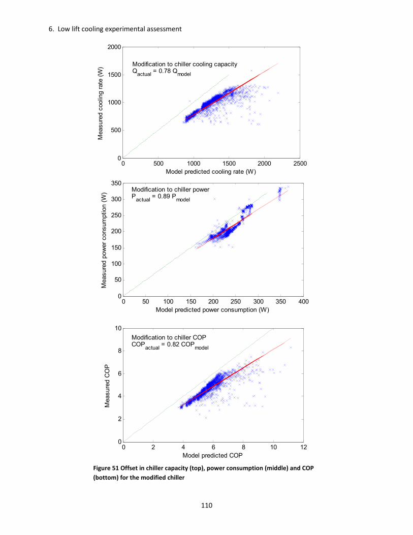
6. Low lift cooling experimental assessment
110
0 50 100 150 200 250 300 350 4000
50
100
150
200
250
300
350Modification to chiller powerPactual
= 0.89 Pmodel
Model predicted power consumption (W)
Measured power consumption (W)
0 500 1000 1500 2000 25000
500
1000
1500
2000
Modification to chiller cooling capacityQactual
= 0.78 Qmodel
Model predicted cooling rate (W)
Measured cooling rate (W)
0 2 4 6 8 10 120
2
4
6
8
10
Modification to chiller COPCOP
actual = 0.82 COP
model
Model predicted COP
Measured COP
Figure 51 Offset in chiller capacity (top), power consumption (middle) and COP
(bottom) for the modified chiller

6. Low lift cooling experimental assessment
111
Figure 53 Two refrigerant loop branches serving the air -side indoor unit and the BPHX. The plant-side chilled
water loop is also shown
BPHX refrigerant
return
BPHX refrigerant
supply
Air-side indoor
unit supply
Air-side indoor
unit return
Radiant floor chilled
water supply
Radiant
floor chilled
water return
Water
pump
BPHX
Figure 52 Condenser, condenser fan and compressor (normally the electronics, including the compressor
inverter, is cooled by the condenser air stream)
Condenser fan
and condenser
Compressor encased in
insulation
Power conditioning,
DC bus, inverters

6. Low lift cooling experimental assessment
112
Figure 55 Complete LLCS radiant concrete-core floor test chamber
Warmboard floor (prior to
concrete installation)
Air-side
evaporator
Radiant floor
manifold
PEX pipe embedded
in Warmboard
Switch
relay box
Internal loads
Wall separating climate and test chambers
Figure 54 Chilled water loop distribution, including radiant floor manifold, PEX pipe loops, Warmboard sub-floor.
The air-side indoor unit evaporator is also shown.
Mixing fan (and
internal load)
Internal loads
Radiant
concrete
floor

6. Low lift cooling experimental assessment
113
6.1.2 Conventional, variable capacity split-system air conditioner
A conventional split-system air conditioner (SSAC) was installed in the test chamber as a
baseline comparison to the LLCS. This system consisted of an off-the-shelf Mitsubishi MUZ-
A09NA-1 outdoor unit and an MSZ-A09NA indoor unit – an air-heated, finned-tube evaporator.
The system is a high efficiency SSAC with a seasonal energy efficiency ratio (SEER) of 16
BTU/Wh [Mitsubishi 2006]. The same MUZ-A09NA-1 outdoor unit serves both the LLCS radiant
concrete floor system and the conventional SSAC. This ensures that the performance of the
two systems can be directly compared. The only differences between the systems are the
evaporators and the controls. The SSAC used an air-heated evaporator, thermostatic control,
and Mitsubishi’s internal proprietary expansion valve, compressor speed and condenser fan
speed controls. The LLCS uses a BPHX liquid evaporator, predictive pre-cooling control, and a
constant superheat control over the expansion valve. All other components and aspects of the
two systems are identical, including the variable speed compressor, variable speed condenser
fan, their inverters and the corresponding efficiencies. Figure 56 shows the configuration of the
SSAC. Under SSAC operation, the valves in the refrigerant lines serving the BPHX are closed
and the valves to the air-heated evaporator are open.
CONDENSER
ELECTRONIC
EXPANSION VALVE
COMPRESSOR
FROM BPHX
(CLOSED)
TO BPHX
(CLOSED)
EVAPORATOR
TEST CHAMBER CLIMATE CHAMBER
LEV
Figure 56 Split-system variable capacity air conditioner that uses the same outdoor unit as the LLCS

6. Low lift cooling experimental assessment
114
6.1.3 Thermal input systems: climate chamber and internal loads
Two other important systems for the LLCS test chamber include an HVAC system serving the
climate chamber used to simulate outdoor temperature variations, and simulated internal
thermal loads. These are described below.
The condenser (the same for both systems) is located in the climate chamber, adjacent to the
test chamber, as described in chapter 4. The condenser air inlet temperature, a variable in the
system performance, is equal to the climate chamber air temperature, the equivalent of
outdoor air temperature (OAT) in the system models. To simulate the performance of the LLCS
and SSAC in different climates, the climate chamber air temperature was controlled by a stand-
alone constant volume HVAC system. A schematic of the climate chamber HVAC system from
its Landis & Gyr control interface is shown in Appendix B.1.
This system controlled the return air temperature set point of air leaving the climate chamber.
To ensure the return air temperature closely approximated climate chamber air temperature,
fans were run continuously inside the climate chamber to mix the air. The return air
temperature set point could be scheduled, through time-of-day schedules, to follow a desired
hourly air temperature schedule. The control program for the climate chamber HVAC system
was re-tuned to provide fast response to changes in climate temperature set point and
disturbances, such as the chiller turning on and off and rejecting heat from the condenser. PID
loops for the system cooling coil control valve, electric heating element, and supply air
temperature set point were tuned to provide a stable response to disturbances within a few
minutes. The control program for the climate chamber HVAC system, which was modified from
an existing control program, is included in Appendix B.1.
Because it was impractical to perform year-long or even cooling season long tests of both
systems, a choice of climate temperature control had to be made that would be representative
of system performance over a period of time in a particular climate. Typical meteorological
year (TMY) weather files are the standard for assessing building energy performance in a given
climate. EnergyPlus weather (EPW) files are based on TMY data and supplemented with
additional analysis. EnergyPlus contains a weather data conversion tool that can generate
hourly weather data for a typical week over a selected period of time. This tool uses a heuristic,
statistical method to compare the climate data statistics over the whole period to statistics of
real, measured weeks within that period to identify a typical week [Crawley et al 1999].
Pre-processed data for seasonal typical and extreme weeks are included within EPW weather
files for a given location, including typical weeks for summer (June-August), fall (September-
November), winter (December-February) and spring (March-May). The EPW typical summer
week for two climates was chosen as a basis for comparison of the LLCS to the split-system AC.
The performance of the LLCS and SSAC was tested for the typical summer week in Atlanta,
Georgia. The LLCS and SSAC will also be compared under a typical summer week for Phoenix,
Arizona and possibly other climates, but this data is not yet available for publication. Testing in
one climate requires two week-long tests, with a few days of advanced operation to achieve

6. Low lift cooling experimental assessment
115
steady-periodic temperature response, or one week for each combination of system and
location. The climate chamber air temperature set points were taken directly from the EPW
files for the typical summer week in Atlanta, Hartsfield-Jackson airport and Phoenix, Deer Valley
airport. These week-long zone air temperature set points are shown in Figure 57.
For each of the two tests, programmed internal loads were placed inside the chamber to
simulate sensible thermal loads from people, lights, and equipment. These thermal loads were
constructed from incandescent light bulbs, in some cases installed inside opaque plastic
enclosures. Two light bulbs were installed on the ceiling of the chamber to simulate lighting
loads. One 75 Watt light bulb was placed in each of two opaque plastic enclosures to simulate
the sensible thermal loads from two occupants. The bulbs were placed in the opaque plastic
enclosure so that visible and near infrared light from the light bulb would be converted to
infrared radiation and convective heat transferring from the surface of the enclosure. Light
bulbs were placed in two additional plastic enclosures to simulate equipment loads. These
enclosures were left open at the top to approximate a higher mix of convective load relative to
radiative loads for electrical equipment. More information on these simulated internal loads is
presented in Appendix B.1.
A ceiling fan was also installed in the chamber and measured as part of the internal loads. This
fan was installed to create air movement inside the chamber and simulate the action of mixing
created by the DOAS, equipment fans, and people moving around. It may be argued that this
ceiling mixing fan should be considered as part of the LLCS because it causes air movement and
improves the performance of the LLCS. On the other hand, an LLCS with a DOAS or with cooling
from above may not need this ceiling mixing fan. The ceiling fan used for experiments was a
very low efficiency fan, consuming around 30 Watts for as little as 200 CFM of flow. Because
the fan should not be necessary for a typical radiant concrete-core cooling system, or TABS, its
power consumption has not been included in the LLCS system power consumption. However,
the fan is measured and counted as an internal load on the test chamber.

6. Low lift cooling experimental assessment
116
0 20 40 60 80 100 120 140 160
20
25
30
35
40
Temperature (C)
Hours
Atlanta typical summer week OAT
0 20 40 60 80 100 120 140 160
20
25
30
35
40
Temperature (C)
Hours
Phoenix typical summer week OAT
Figure 57 Typical summer week hourly outdoor air temperature (OAT) schedule for Atlanta and Phoenix
Two different types of internal load schedules were considered for testing, standard efficiency
loads and high-efficiency loads. The equipment and lighting loads were selected based on the
loads used in [Armstrong et al 2009b], and the occupant associated loads were chosen based
on an assumption of two occupants with only sensible loads included. Light bulbs with
different power consumption were installed in each of the three types of loads to create these
two load schedules. Table 6 shows the break-down of internal loads by type - occupants,
lighting and equipment - and the load densities. The loads are programmed such that at 8:00
am one occupant load, the lighting load, and half the equipment loads turn on, at 9:00 am all
the loads turn on, at 5:00 pm one occupant load and half the equipment loads turn off, and at
6:00 pm all the loads turn off until the next day. Over weekends, the loads remain off. This
schedule is meant to simulate a typical office weekly occupancy schedule in which two
employees share the office, one arrives at 8:00 am and departs at 5:00 pm, one arrives at 9:00
am and departs at 6:00 pm, and both stay home on the weekends. The simulated internal loads
are shown in Figure 58. The weekday load schedules for both the high efficiency and standard
efficiency loads are shown in Figure 59.

6. Low lift cooling experimental assessment
117
Table 6 Internal load distribution and density
Load
Standard
efficiency
(W)
Standard
efficiency
(W/sqft)
High
efficiency
(W)
High
efficiency
(W/sqft)
2 People 160 0.8 160 0.8
Lights 220 1.1 120 0.6
Equipment 300 1.5 120 0.6
Figure 58 Lighting, simulated equipment and occupant loads
5 10 15 200
100
200
300
400
500
600
700
800
Load (W)
Hour
Standard efficiency load schedule
Peak load density = 3.4 W/sqft
5 10 15 200
100
200
300
400
500
600
700
800
Load (W)
Hour
High efficiency load schedule
Peak load density = 2 W/sqft
Figure 59 Internal load schedule for standard efficiency and high efficiency loads

6. Low lift cooling experimental assessment
118
The standard efficiency internal load schedule was applied to the tests for Atlanta climate
conditions. This choice was made in part to match the capacity of the chiller, which is oversized
for the LLCS test chamber when subjected to the high efficiency load schedule and the Atlanta
typical summer week. The high efficiency internal load schedule will be applied to future
testing under Phoenix climate conditions. For standard efficiency internal loads under Phoenix
conditions the cooling capacity of the radiant floor – particularly the thermal storage capacity of
the concrete slab – is undersized for the total thermal load. Working within the constraints of
the installed systems and their capacities, comparative testing of the LLCS and SSAC was
performed subject to Atlanta typical summer week climate conditions with standard efficiency
internal loads.
There are two other important thermal inputs to the experimental system. First, the air
temperature in the adjacent zone, referred to as AAT in chapters 4 and 5, also effects the zone
temperature response. The adjacent zone refers to the laboratory in which the LLCS test
chamber and climate chamber is built. The AAT was maintained around a constant 23 Celsius
during the duration of the tests. This was done to ensure that the dominant heat transfer
occurred between the test chamber zone and the climate chamber zone, and not the
laboratory or adjacent zone. The heavily insulated surfaces separating the adjacent zone from
the test chamber zone and the very low temperature differences between the zones limited the
impact of the adjacent zone on the testing.
The second important thermal consideration is the relative humidity inside the test chamber.
The radiant concrete floor cooling system is intended only to perform sensible cooling within
the context of LLCS. A separate DOAS, as described in chapter 2, is necessary to perform latent
cooling. Consequently, the experiments required that the relative humidity inside the chamber
be kept as low as possible, with the dewpoint temperature well-below any surface
temperature, to prevent latent cooling from occurring. The air inside the climate chamber and
the air in the adjacent zone were continuously dehumidified to prevent moisture from entering
the test chamber. No sources of moisture were present inside the chamber. This limited the
amount of latent cooling that occurred. However, dewpoint temperature occasionally rose
above certain surface temperature for both the LLCS and the SSAC, and both systems
performed some latent cooling during testing.
For the SSAC, the condensate was collected and measured to account for latent cooling. After
testing, the average measured COP of the unit from the test and the heat of vaporization of
water was used to convert the mass of condensate water into an estimate of the SSAC energy
consumption for latent cooling. Energy performance comparisons of the LLCS and SSAC will be
made for the two systems with and without deducting this latent energy consumption from the
SSAC energy consumption. Because the LLCS most likely performed some uncontrolled latent
cooling as well, though immeasurable, it is not clear whether it is more fair for comparison to
deduct the SSAC latent cooling energy consumption or not. Both approaches will be presented.
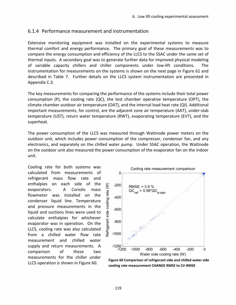
6. Low lift cooling experimental assessment
119
6.1.4 Performance measurement and instrumentation
Extensive monitoring equipment was installed on the experimental systems to measure
thermal comfort and energy performance. The primary goal of these measurements was to
compare the energy consumption and efficiency of the LLCS to the SSAC under the same set of
thermal inputs. A secondary goal was to generate further data for improved physical modeling
of variable capacity chillers and chiller components under low-lift conditions. The
instrumentation for measurements on the systems is shown on the next page in Figure 61 and
described in Table 7. Further details on the LLCS system instrumentation are presented in
Appendix C.3.
The key measurements for comparing the performance of the systems include their total power
consumption (P), the cooling rate (QC), the test chamber operative temperature (OPT), the
climate chamber outdoor air temperature (OAT), and the internal load heat rate (QI). Additional
important measurements, for control, are the adjacent zone air temperature (AAT), under-slab
temperature (UST), return water temperature (RWT), evaporating temperature (EVT), and the
superheat.
The power consumption of the LLCS was measured through Wattnode power meters on the
outdoor unit, which includes power consumption of the compressor, condenser fan, and any
electronics, and separately on the chilled water pump. Under SSAC operation, the Wattnode
on the outdoor unit also measured the power consumption of the evaporator fan on the indoor
unit.
Cooling rate for both systems was
calculated from measurements of
refrigerant mass flow rate and
enthalpies on each side of the
evaporators. A Coriolis mass
flowmeter was installed on the
condenser liquid line. Temperature
and pressure measurements in the
liquid and suctions lines were used to
calculate enthalpies for whichever
evaporator was in operation. On the
LLCS, cooling rate was also calculated
from a chilled water flow rate
measurement and chilled water
supply and return measurements. A
comparison of these two
measurements for the chiller under
LLCS operation is shown in Figure 60.
Figure 60 Comparison of refrigerant side and chilled water side
cooling rate measurement CHANGE RMSE to CV-RMSE
-1200 -1000 -800 -600 -400 -200 0-1200
-1000
-800
-600
-400
-200
0
RMSE = 3.9 %QC
ref = 0.99*QC
w ater
Water side cooling rate (W)
Refrigerant side cooling rate (W)
Cooling rate measurement comparison

6. Low lift cooling experimental assessment
120
Table 7 Low lift chiller system sensor labels
Label Sensor description
Ts Suction refrigerant temperature
Td Discharge refrigerant temperature
Tcnd Refrigerant condensing temperature
Tcnd,liq Condenser outlet liquid refrigerant temperature
Txvi Expansion valve inlet refrigerant temperature
Txvo Expansion valve outlet refrigerant temperature
Thxi Brazed plate heat exchanger inlet refrigerant temperature
Thxo Brazed plate heat exchanger outlet refrigerant temperature
Tcnd,air,in Condenser inlet air temperature
Tevp Refrigerant evaporating temperature (not shown, installed on indoor unit of split-system)
∆Tcnd,air Condenser air temperature difference
Ps Suction refrigerant pressure
Pd Discharge refrigerant pressure
Pxvi Expansion valve inlet refrigerant pressure
Pxvo Expansion valve outlet refrigerant pressure
refm& Refrigerant mass flowrate
Wunit Total power to the outdoor unit, including inverters, condenser fan and compressor
W3∅,cmp Three phase power from the inverter to the compressor
RWT Chilled water return temperature
SWT Chilled water supply temperature
" Chilled water volumetric flowrate
WQI Total power to the internal loads
Wp Total power to the chilled water pump
Thxo
Thxi
Ps, Ts
Pxvo, Txvo Pxvi, Txvi
LEV
Pd, Td
Tcnd,liq
Tcnd
∆Tcnd,air
refm&
W3∅,cmp
Wunit
Tcnd,air,in
" RWT
SWT
Wp
WQI
Figure 61 Low lift chiller system performance measurement instrumentation
6. Low lift cooling experimental assessment
121
The temperature measurements for the LLCS test chamber, including OPT, OAT, AAT, and UST
were made using the same surface and air temperature measurements described in Chapter 4
and shown in Figure 29. For an installation in an occupied building, a globe temperature
measurement may be substituted for the multiple air and surface temperature measurements
as an approximation to OPT. However, for purposes of accurate and fair comparison of thermal
performance, extensive monitoring of air and surface temperatures was performed for this
research. A separate Wattnode power meter was used to measure the power consumption
and thus heat dissipated by the simulated loads from people, lights and equipment.
Additional temperature sensors on the chilled water loop and the evaporator provided
measurements of RWT and EVT. The refrigerant temperature at the inlet and outlet of the
BPHX was measured from which the refrigerant superheat could be calculated for controlling
the electronic expansion valve. Four pairs of pressure and temperatures at each of the key
vapor compression cycle points were measured, at the suction port, discharge port, expansion
valve inlet, and expansion valve outlet. Additional measurements included the refrigerant
condensing and evaporating temperatures at the midpoints of the corresponding heat
exchangers, three phase power consumption of the rolling-piston compressor, condenser air
temperature, condenser air temperature difference, and evaporator inlet air temperature and
humidity. The compressor speed, condenser fan speed, and expansion valve positions were
set, and thus known, through the control system for the LLCS.
6.2 LLCS testing procedure
The following process was executed to generate performance data for the LLCS and the SSAC
from which to compare energy consumption and thermal performance:
1. The outdoor climate chamber was continuously controlled to achieve an hourly air
temperature schedule defined by a typical summer week for a selected climate as
shown in Figure 57.
2. The internal loads were programmed to follow one of the daily load profiles shown in
Figure 59 during weekdays. The internal loads remained off during the weekends.
3. The LLCS radiant concrete floor cooling system was operated for one week, including
one weekend, after a three day initialization period. It was programmed to maintain
operative temperature between 19.5 and 25 Fahrenheit, based on [ASHRAE 2007a]
during an occupied period from 8:00 am to 6:00 pm. This required the following steps:
a. A Matlab script implementing the predictive pre-cooling optimization algorithms
shown in Figures 45 and 46 was initiated.
b. At every hour, a pattern search predicted the near-optimal compressor speed
and condenser fan speed schedules for the next 24 hours and set the
6. Low lift cooling experimental assessment
122
compressor speed and condenser fan speed to the optimal set point for the first
hour.
c. The chilled water pump operated at a constant speed any time the compressor
and condenser fan were running, otherwise it was shut off.
d. The predictive pre-cooling control of the LLCS radiant concrete floor cooling
system was run for at least three days prior to gathering test data for
comparison. This allowed the system to achieve a steady-periodic temperature
response.
e. LLCS test data was gathered for one week. Data was recorded at one minute
intervals for all of the sensors described in chapters 4 and 6. The week spanned
a complete weekend so that the test included the energy required to cool down
the concrete floor after a weekend of floating up to a higher temperature.
4. After completion of the LLCS test, the test chamber was allowed to achieve thermal
equilibrium prior to conducting SSAC tests. Particularly, concrete temperatures were
allowed to return to equilibrium with the zone air temperatures.
5. The refrigerant charge was balanced by observing the state of the refrigerant exiting the
condenser into a receiver through two sight glasses. The valves on the entering side of
the evaporator were left open, allowing refrigerant to be drawn from the other system,
until the bottom of the receiver filled with liquid and the top of the receiver remained
all or partially vapor over a wide range of compressor speeds. Thus, both systems
operated under near zero sub-cooling for most compressor speeds.
6. The SSAC was operated for one week after an initialization period to achieve steady-
periodic temperature response. The system was controlled to meet an average air
temperature equal to the average operative temperature achieved by the LLCS for each
corresponding day of operation. The off-the-shelf system could not be controlled to
achieve operative temperature, because it operating under thermostatic control relative
to its on-board air temperature sensor. However, the operative temperatures were
compared after testing to ensure that a consistent level of comfort, based on daily mean
operative temperature, was achieved in both cases.
This procedure was followed to test the LLCS and the SSAC under Atlanta typical summer week
climate conditions with standard efficiency internal loads. In the near future, the systems will
be tested under Phoenix typical summer week conditions with high efficiency internal loads.
These two tests were chosen to sample the range of conditions under which LLCS may be
applied and to provide appropriate thermal loads relative to the capacity of the systems. More
testing will be performed with the chamber in future research.

6. Low lift cooling experimental assessment
123
6.3 LLCS energy and thermal performance assessment
This section will compare the sensible cooling energy and thermal comfort performance of the
LLCS with predictive pre-cooling control to an SSAC subjected to the experimental tests
described in section 6.1 and 6.2. As explained in chapter 2, simulations suggest that total
cooling energy savings of LLCS, including sensible and latent cooling energy, relative to DOE
benchmark building systems typically average around 60 percent of the total cooling energy
consumption for medium office buildings.
The tests conducted for this research only investigate the sensible cooling energy savings
provided by predictive control of the chiller pre-cooling the concrete radiant floor. The savings
due to de-coupling of latent and sensible loads and more efficient dehumidification have not
been investigated. Estimated latent cooling savings for an efficient DOAS vary by climate and
building type. Mumma and Shank [2001] estimated only an 11 percent latent cooling energy
savings per unit of outside air for a DOAS with enthalpy recovery and a run around heat
exchanger relative to a conventional VAV system in Atlanta. However, they did not include
(and noted it) that DOAS typically reduce outdoor air requirements relative to a VAV system.
More research is necessary to evaluate potential latent cooling energy savings for different
configurations of DOAS and dehumidification systems in combination with LLCS, by building and
by climate.
The base line SSAC system to which the LLCS is compared is most similar to the VAV system
with a variable speed chiller in [Armstrong et al 2009b, Katipamula et al 2010]. However, the
VAV system from [Katipamula et al 2010] included an air-side economizer and larger specific
fan power than the SSAC. In addition, the LLCS included a refrigerant side economizer, ideal
TES, and a different chiller performance map.
Figures 62 and 63 show the results of testing the LLCS and the SSAC under Atlanta typical
summer week climate conditions subject to standard efficiency internal loads. The figures
show the temperature response, including outdoor air temperature (OAT), adjacent zone air
temperature (AAT), operative temperature (OPT), under-slab temperature (UST) and return
water temperature (RWT). Also shown are the internal load heat rate (QI), system cooling rate
(QC), and system power (P).
In Figure 62, it may be observed that the LLCS runs for more hours but at lower power
consumption, and in advance of the occupied period, than the SSAC, as shown in Figure 63.
This is a key characteristic of low lift cooling. The cooling load is spread out over time and
cooling is delivered to TES in advance, allowing the chiller to run at lower speeds and over night
when lower condensing temperatures are possible. The displayed cooling rate under SSAC
operation is not perfectly accurate. The cooling rate measurement does not include cooling
during transient conditions, which are significant, because the refrigerant mass flow rate used
for calculating QC was not measureable during transient conditions. This is a typical problem
caused by two phase flow through the Coriolis mass flow meter used to measure mass flow
rate.

6. Low lift cooling experimental assessment
124
0 20 40 60 80 100 120 140 160
10
20
30
Temperature (C)
OAT
AAT
OPT
UST
RWT
0 20 40 60 80 100 120 140 160-1500
-1000
-500
0
500
1000
Thermal Load (W)
Internal load (W)
Cooling rate (W)
0 20 40 60 80 100 120 140 1600
100
200
300
400
hour
Power (W)
LLCS power
consumption (W)
Figure 62 Results for the LLCS under Atlanta climate and standard loads. For the duration of the test, the top
graph shows the outdoor air temperature (OAT), adjacent zone air temperature (AAT), zone operative
temperature (OPT), under-slab temperature (UST) and return water temperature (RWT); the middle graph
shows the internal load heat rate and the cooling rate; and the bottom graph shows the LLCS power
consumption at each hour.

6. Low lift cooling experimental assessment
125
0 20 40 60 80 100 120 140 160
20
25
30
35
Temperature (C)
OAT
AAT
OPT
UST
0 20 40 60 80 100 120 140 160-1500
-1000
-500
0
500
1000
Thermal Load (W)
Internal load (W)
Cooling rate (W)
0 20 40 60 80 100 120 140 1600
100
200
300
400
hour
Power (W)
Split-system AC power
consumption (W)
Figure 63 Results for the SSAC under Atlanta climate and standard loads. For the duration of the test, the top
graph shows the outdoor air temperature (OAT), adjacent zone air temperature (AAT), zone operative
temperature (OPT), under-slab temperature (UST) and return water temperature (RWT); the middle graph
shows the internal load heat rate and the cooling rate; and the bottom graph shows the LLCS power
consumption at each hour. Note: the cooling rate measurement does not include cooling during transient
conditions, which are significant, because the refrigerant mass flow rate used for calculating QC was not
measureable during transient conditions. (This is typical of Coriolis mass flow meters with significant two
phase flow)

6. Low lift cooling experimental assessment
126
A comparison of the energy performance of the LLCS system to the SSAC is shown in Table 8.
Table 8 presents the relative performance of the LLCS and SSAC with regard to cooling
delivered, energy consumed, average COP and EER, and average pressure ratio over the
duration of the test. The energy consumption data is reliable and accurate, based on simple
power measurements. Comparing the other data requires caution. As previously mentioned,
the cooling rate could not be measured continuously during the test due to the limitations of
the refrigerant mass flow meter. Consequently, the total cooling delivered under SSAC
operation is underestimated. The COP and EER estimates can be made in two ways. The
average of the instantaneous COP during the test, while it was measurable, provides one
estimate of average COP while the total measurable cooling delivered divided by the total
energy consumed provides a second. The actual average COP of the SSAC during testing lies
somewhere in between these two estimates. Therefore, only a range in percent improvement
in COP and EER can be inferred.
Table 8 Comparison of SSAC and LLCS performance
SSAC
a LLCS
Percent
difference
Cooling delivered (Whth) -38,927a -48,002 23%a
Measured energy consumed (Whe) 14,645 10,982 -25%
Energy consumed after deducting
latent cooling energy (Whe) 14,053b 10,982b -22%
Average COP (Wth / We) 2.66-4.2a 4.7 12-77%a
Average EER (Btu/Wh) 9.1-14.3a 16.0 12-77%a
Average pressure ratio (kPa/kPa) 1.96 1.70 -13%
a. SSAC cooling rate is under-estimated due to limitations of the refrigerant mass flow meter
b. The latent energy consumption can only be estimated for SSAC operation based on measurement of condensate
water. The LLCS also may have performed some latent cooling.
Two baseline SSAC cases are considered, one which includes the total measured energy
consumption of the SSAC, and one for which the latent cooling energy associated with the
measured condensate water has been deducted from the measured consumption. Both of
these are compared to the measured energy consumption of the LLCS. The latent cooling
energy consumption of the LLCS was not estimated, because it was not possible to measure,
and thus it was not deducted from the LLCS power consumption.
The results in Table 8 show that LLCS sensible cooling energy savings are indeed significant. The
actual measured energy consumption of the LLCS was 10,982 Wh for a typical summer week in
Atlanta (based on the TMY data) subject to standard efficiency internal loads. The SSAC
consumed 14,645 Wh for the same set of conditions. This is an energy savings of 25 percent.
After deducting latent cooling energy from the SSAC consumption only, the energy savings is 22

6. Low lift cooling experimental assessment
127
percent. However, It may be argued that the deduction of latent cooling energy from only SSAC
unfairly penalizes the LLCS. The LLCS may have performed latent cooling also though it could
not be measured. Comparing the LLCS to SSAC energy consumption where latent cooling
energy has been deducted from only the SSAC may result in bias favoring the latter.
Figure 64 shows the operative temperatures (OPT) for each day of the week under the SSAC
and LLCS operation. The LLCS OPT rises dramatically over the course of a typical day. In the
data for Tuesday, it rose from 19 Celsius at 8:00 am to 25 Celsius at 5:00 pm. This is below the
limits for temperature variation over time in [ASHRAE 2007a], which allows a rise of 3.3 Celsius
over four hours. However, some may argue that a six degree rise over the day is still too much,
and that a three to four degree rise is the limit of acceptability based on HVAC designers’
experience [Koschenz and Dorer 1999]. The vertical air temperature difference within the zone
was less than one degree Celsius in both cases, in large part due to the presence of a ceiling
mixing fan which was included to account for the effects of cooling from above and below in a
full-scale concrete-core system and air movement cause by a DOAS.
The mean temperatures over the course of the full day are also shown in Figure 64 and are
comparable for the LLCS and the SSAC over all of the days. Limitations on control over the SSAC
made it impossible to exactly match the operative temperatures achieved by the LLCS and the
SSAC. The SSAC is controlled by zone air temperature alone. An estimate of the average mean
radiant temperature over a day had to be made from which a zone air set point could be
chosen that would yield an operative temperature under SSAC operation comparable to the
LLCS over each day.
The end result of the Atlanta tests are that the LLCS shows significant energy savings, around 25
percent, relative to the split system AC while still achieving comfortable operative
temperatures between 19.4 and 25 Celsius over the day. The drift in operative temperature
over a day is significant for the LLCS, and exacerbated by high internal loads, but is acceptable
0 5 1018
19
20
21
22
23
24
25
26
OPTLLCS
= 23.4
OPTSPLIT
= 22.8
hour
temperature (C)
Monday
0 5 1018
19
20
21
22
23
24
25
26
OPTLLCS
= 23
OPTSPLIT
= 22.7
hour
Tuesday
0 5 1018
19
20
21
22
23
24
25
26
OPTLLCS
= 22.9
OPTSPLIT
= 22.8
hour
Wednesday
0 5 1018
19
20
21
22
23
24
25
26
OPTLLCS
= 22.9
OPTSPLIT
= 22.8
hour
Thursday
0 5 1018
19
20
21
22
23
24
25
26
OPTLLCS
= 23.1
OPTSPLIT
= 22.7
hour
Friday
OPTLLCS
OPTSPLIT
Figure 64 Comparing zone operative temperatures (OPT) for the LLCS and split system AC operation

6. Low lift cooling experimental assessment
128
for the standard efficiency internal loads tested. These results are comparable to the estimated
annual energy savings, 28.8 percent, for the LLCS simulated in [Katipamula et al 2010] for
Atlanta subject to standard efficiency internal loads.
However, the differences in the basis for these two savings estimates should be carefully noted.
Most importantly, the savings presented in this research are based on the real life performance
of an LLCS subject to a typical summer week in Atlanta. The savings in [Katipamula et al 2010]
are based on simulations of a theoretical LLCS subject to a year of Atlanta conditions. y
Furthermore, the base line VAV system in [Katipamula et al 2010] includes an air-side
economizer and higher specific fan power, while the LLCS system includes a refrigerant side
economizer, ideal TES, and a different chiller performance map.
The limitations of the LLCS test chamber must also be acknowledged in interpreting the energy
performance results. Because the test chamber is quite small, the chiller is somewhat oversized
for the test chamber loads. The internal loads were somewhat oversized in an attempt to
match the chiller, but this also results in a mismatch between the concrete floor storage
capacity, cooling capacity and the test chamber thermal loads. This mismatch inhibits the
performance of the LLCS by requiring more cooling, and allowing less load shifting, than would
be required for a well-matched system. Also, the test chamber is a single story zone, where
cooling energy losses from the bottom of the slab do not contribute to cooling of a space below
as they would in a multi-story concrete-core system. As a result, the LLCS provides more
cooling to the LLCS test chamber concrete floor than it would in a multi-story application.
Consequently, the LLCS system performance potential is somewhat constrained by the
limitations of the LLCS test chamber, and the results presented here may underestimate the
achievable sensible cooling energy savings.
6.4 Simulating LLCS predictive pre-cooling control applied to SSAC and RCP
In addition to measuring the actual system energy consumption of a conventionally controlled
SSAC and an LLCS with a radiant concrete floor, simulations were performed of other possible
LLCS configurations that use SSAC or radiant ceiling panels (RCP). The goal of these simulations
were to identify how much energy savings could be achieved by applying predictive pre-cooling
control for low-lift chiller or air conditioner operation without the use of the concrete-core
radiant floor system. The as-built LLCS configuration with concrete radiant floor cooling will
here be referred to as an LLCS thermo-active building system (TABS).
Five different system configurations, described below, were simulated to assess and compare
predictive control to achieve low-lift cooling using the TABS system, the split-system air
conditioner (SSAC), and a radiant ceiling panel (RCP). These simulations were performed in the
Matlab environment using the modeling methods described in chapters 2 and 3 and the control
algorithm from chapter 4. The temperature response of the zone for all of these cases was
modeled using the same temperature-CRTFs, which are the same as those used for the
experimental assessment previously described in chapter 4. The system models for each case
were different. Calibrated data-driven models of the LLCS chiller performance, developed for

6. Low lift cooling experimental assessment
129
predictive control of the LLCS test chamber, were used for cases three through five. Un-
calibrated data-driven models of the SSAC performance based on the data from chapter 3 were
used for cases one and two, because calibration data was not collected for the SSAC. The five
systems simulated are as follows:
1. Base case SSAC under thermostatic control (BASE-SSAC). The SSAC performance was
modeled using the air conditioner performance described in chapter 3, but it was not
calibrated to the as-built SSAC performance The SSAC studied in chapter 3 was the same
make and model as that installed in the chamber, but not the same physical system. As a
result, the actual performance of the SSAC in the test chamber differed from that of the
curve-fit models from chapter 3. There is insufficient data to calibrate the SSAC model from
chapter 3 to the as-built SSAC performance in the LLCS test chamber. Further data may be
collected to calibrate the SSAC model, which would require more data on evaporator
cooling rate, compressor speed and condenser fan speeds over a range of operating
conditions. The zone air temperature setpoint for the thermostatic control was 23 Celsius,
as in the experiments.
2. SSAC with predictive control (LLCS-SSAC). The SSAC performance was modeled as described
above under BASE-SSAC. The same predictive pre-cooling control algorithm applied to the
experimental LLCS-TABS system was used, as described in chapter 5.
3. TABS with predictive control (LLCS-TABS). The chiller system performance was modeled
using the chiller performance map measured from the experimental test stand as described
in chapter 3, but calibrated to the as-built performance of the chiller serving the concrete
floor as described in chapter 6.
4. TABS with predictive control and a higher capacity radiant floor (LLCS-TABS+). This case was
simulated to project the potential savings for an improved radiant concrete-core floor
design, in which the floor had reduced pipe spacing, higher capacity, and less resistance
between the bottom of the concrete and the chiller water loop. The temperature
difference between the chilled water and the bottom of the concrete pavers was assumed
to be half of that observed with the existing floor. Improvements to the thermal storage
efficiency of the concrete floor, by adding insulation underneath, were not modeled. The
chiller performance was modeled as described above under LLCS-TABS.
5. RCP with predictive control (LLCS-RCP). An RCP was modeled based on the radiant ceiling
panel model described in [Armstrong et al 2009a]. The RCP total heat transfer coefficient
was assumed to be 13.2 W/m2-K based on the results of [Causone et al 2009]. The entire
test chamber ceiling, 3.65 m by 5.2 m, was assumed to be covered with RCP. The return
water temperature was calculated using equation 20a in [Armstrong et al 2009a], which is a
simple heat exchanger effectiveness-NTU relation between the zone air and the chilled
water, using a single air temperature on the zone air side. The evaporating temperature
was calculated based on the superheat control law implemented in the as-built system
instead of with the flooded evaporator model described in [Armstrong et al 2009a]. The

6. Low lift cooling experimental assessment
130
chiller performance was modeled as described above under LLCS-TABS, but using the return
water temperature and subsequent evaporating temperature calculated for the RCP.
Each case was simulated under a typical summer week in Atlanta subject to standard efficiency
internal loads. Forecasts of internal loads and outdoor temperature variations were perfect,
because the forecasts rather than actual measured data from the experimental chamber were
used for simulation. The total energy consumption over a typical summer week for each of
these cases was calculated based on simulations of each system in Matlab. A summary of these
findings is presented in Table 9.
Table 9 Energy consumption and relative savings from simulations of SSAC, TABS and RCP under with low-lift
predictive pre-cooling control
BASE-
SSAC
LLCS-
SSAC
LLCS-
TABS
LLCS-
TABS+
LLCS-
RCP
Cooling delivered (Wh) -47,940 -39,920 -53,200 -52,010 -39,420
Simulated energy (Wh) 11,110 8,038 11,072 10,824 5,285
Measured energy (Wh) 14,053 n/a 10,982 n/a n/a
Error in simulation 20.9% n/a -0.8% n/a n/a
Savings relative to
simulated base case base 27.6%
base 2.2% 52.3%
The first important point about the results shown in Table 9 is that the simulated SSAC does not
accurately model the as-built SSAC. There is a 20.9 percent difference between the measured
SSAC system performance and the simulated SSAC system performance. This difference may
have the following causes. First, the actual transient performance of the SSAC is not reflected
in its steady-state performance map from chapter 3, which is the model used to simulate SSAC
performance. Second, it is likely that the performance of the as-built SSAC is different from the
SSAC tested in chapter 3, just as the as-built chiller performance was different from the
performance map from chapter 3 and required the calibrations described in section 6.1.1.
Currently, not enough information is available to calibrate the performance map model of the
SSAC to its as-built performance. The same model structure should be applicable to the as-built
SSAC, but the coefficients of the model may be somewhat different than the SSAC tested in
chapter 3.
With these differences in system modeling in mind, the results of the simulations have only
been compared when the same underlying cooling system model has been used for both cases.
Thus, it is reasonable to compare the BASE-SSAC case to the LLCS-SSAC case because the exact
same models were used for both simulations, only the control laws were changed. The same is
true for the LLCS-TABS, LLCS-TABS+, and LLCS-RCP cases to the extent that the TABS+ and RCP
assumptions are achievable and representative of a real system. The same calibrated chiller
performance was used for those three cases.

6. Low lift cooling experimental assessment
131
The following conclusions can be drawn from the results in Table 9. First, by employing
predictive pre-cooling control directly to the SSAC, simulations suggest over 27 percent energy
savings relative to conventional control. These savings are comparable to the measured energy
savings of the LLCS-TABS relative to the SSAC. However, it should not be taken at face value
that an LLCS-SSAC could save the same energy as an LLCS-TABS in any situation. The ability of
the SSAC to achieve the same savings as the TABS under predictive control for the modeled
LLCS test chamber may be the result, in part, of low internal load densities relative to the chiller
capacity. This mismatch results in less need for storing cooling energy in the concrete, and the
SSAC can provide enough pre-cooling despite the fact that it is less effective than the TABS
system at pre-cooling the concrete slab. It may also be affected by the thermal storage
capacity of the slab, which is reduced by losses to below from the concrete-floor of the LLCS
test chamber. This is evident in the amount of total cooling delivered by each case. The TABS
systems provide far more cooling than required to meet the load due to losses from the floor.
The cooling delivered by the TABS system in simulation is roughly 25 percent more than that of
the RCP. This agrees, approximately with the results of a physical model of the concrete floor,
which shows that the losses from the bottom of the floor may range from 15 to 30 percent
depending on the actual thermal conductivity of the concrete, as described in Appendix B.1.
Second, improving the TABS system, represented by the LLCS-TABS+ case, to achieve higher
chilled water temperatures may not achieve significantly greater savings than the LLCS-TABS
case. Only an additional 2.2 percent savings was simulated for the LLCS-TABS+. This is likely
because the chilled water temperatures and evaporating temperatures are only a few degrees
warmer in the LLCS-TABS+ case than in the LLCS-TABS case.
Lastly, the LLCS-RCP system shows significant potential for energy savings over the LLCS-TABS
case for the existing test chamber, with over 50 percent simulated savings relative to LLCS-
TABS. This is primarily the result of significantly higher chilled water temperatures. However,
again, the LLCS-RCP savings are skewed because of the mismatch between the chiller capacity
and the internal loads, as well as the low thermal storage efficiency of the LLCS test chamber.
Better matching of capacity and load and improved concrete-core thermal storage efficiency
should result in more savings from the LLCS-TABS relative to the LLCS-RCP. In the LLCS-RCP
simulated case, the RCP system runs primarily during occupied hours because it can efficiently
meet the loads with higher chilled water temperatures without utilizing passive TES overnight.
In summary, the simulations show that predictive pre-cooling control for low-lift chiller or air
conditioner operation has great potential for energy savings even without a TABS concrete
radiant floor cooling system. Simply applying predictive pre-cooling control to the conventional
SSAC resulted in 27 percent simulated energy savings. More research is needed to confirm and
evaluate the actual energy savings achievable for each of these configurations and many other
LLCS configurations beyond TABS, SSAC, or RCPs.

6. Low lift cooling experimental assessment
132
6.5 Experimental LLCS demonstration in Masdar City
One final component of this research is the construction of a larger LLCS test chamber exposed
to real outdoor climate conditions at Masdar City in the United Arab Emirates (UAE). This
demonstration project was constructed inside a portion of the Masdar field offices on the
Masdar City construction site. Masdar City is a UAE sponsored project to build a net-zero
energy city near Abu Dhabi, UAE. The Abu Dhabi Future Energy Company (ADFEC) has
supported LLCS research with the possibility that, because of its low cooling energy intensity, it
may help enable the development of a net-zero energy city. The need for efficient cooling is
extremely important at Masdar City because cooling dominates electricity demand and daytime
summer temperatures are frequently above 40 Celsius.
The Masdar LLCS test chamber was constructed from three modular building containers in the
corner of the Masdar City field offices. Twenty five centimeters of foam insulation was installed
on the floor of the modules and 15 centimeters of concrete was poured above the slab. Pex
pipe with a pitch of 10 centimeters was embedded in the concrete slab. A system identical to
the system described in Chapter 6 was constructed for the Masdar LLCS test chamber, but is
still not operational. As part of this research, the radiant concrete floor, the low-lift chiller and
base-case SSAC systems were constructed or assembled and sensors for measuring their
performance were installed. Images of the Masdar City LLCS test chamber project are shown in
Figure 65.
At the time of publication, researchers at the Masdar Institute of Science and Technology are
continuing work on this LLCS demonstration project with the goal of making comparative
assessments of LLCS and SSAC system performance. The project will require a number of
advancements from this thesis. Solar loads will need to be inferred from irradiance
measurements and incorporated into the CRTF models. The effects of wind and resulting
variations in infiltration loads may need to be captured in the CRTF models. Real weather
forecasts will be needed for the predictive pre-cooling control optimization. Results from
these experiments are forthcoming.
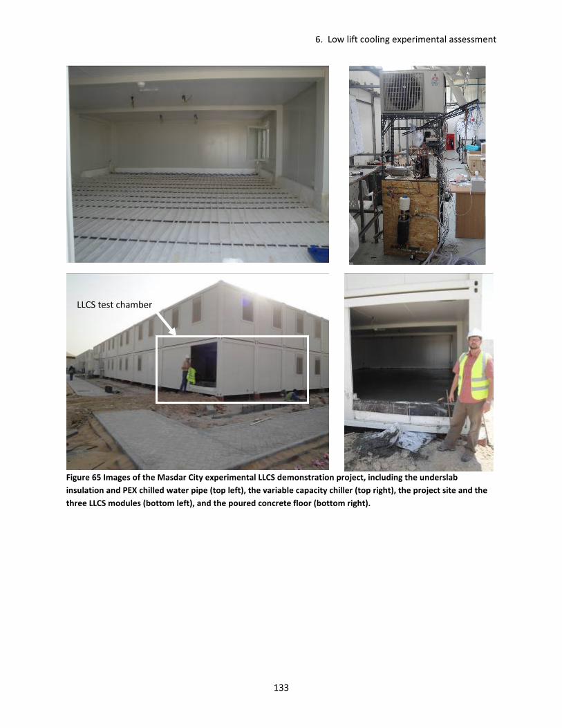
6. Low lift cooling experimental assessment
133
Figure 65 Images of the Masdar City experimental LLCS demonstration project, including the underslab
insulation and PEX chilled water pipe (top left), the variable capacity chiller (top right), the project site and the
three LLCS modules (bottom left), and the poured concrete floor (bottom right).
LLCS test chamber

134
Chapter 7 Conclusion
This chapter will summarize the original contributions presented in this research. This includes
measured energy savings of a low lift cooling system (LLCS) with radiant concrete-core cooling
relative to a split-system air conditioner (SSAC) in a near full scale LLCS test chamber. A
summary of key technical contributions to develop LLCS model-based, predictive pre-cooling
control algorithms will also be presented. The chapter will then describe alternative LLCS
configurations and the barriers to and benefits of implementing LLCS on a large scale. Finally,
future research directions stemming from this work will be explored.
7.1 Original contributions
This research significantly advances knowledge about the implementation, control and
performance of LLCS. A specific LLCS configuration, a variable speed chiller serving a concrete
radiant floor with near-optimal predictive pre-cooling control was implemented and tested.
This included developing the data-driven models and controls necessary to support predictive
pre-cooling control of LLCS based on measured building data. The following achievements are
considered important original contributions of this research.
First, the sensible cooling energy savings of an LLCS concrete core radiant cooling system with
predictive pre-cooling control relative to a high efficiency, variable speed SSAC was tested in an
experimental test chamber for the typical summer week in Atlanta with standard efficiency
internal loads. The measured LLCS sensible cooling energy savings relative to the SSAC was 25
percent of the SSAC typical summer week consumption. These results confirm previous
estimates based on simple simulation models [Katipamula et al 2010] which found 28.8 percent
annual energy savings for a similar (not identical) LLCS system relative to a similar base case
system. Caveats in comparing these two savings estimates are discussed below.
A second major contribution of this work is a methodology for predictive pre-cooling control of
a LLCS radiant concrete core cooling system that includes the thermal response of real building
thermal mass. This methodology includes the use of chiller performance maps, or look-up
tables, and building thermal response models, such as CRTFs, into a pre-cooling control
optimization algorithm. Incorporating the thermal response of real concrete-core thermal mass
into this optimization is a key contribution beyond prior research. This is necessary and
important because the chiller efficiency depends on evaporating temperature, which in turn
depends on chilled water temperature and thus on the state of the pre-cooled thermal mass.

7. Conclusion
135
A third contribution is a detailed data set on the performance of a rolling-piston compressor
heat pump created from experimental measurements to support this and future research. The
heat pump data was used to create curve-fit performance models of a low-lift chiller valid
under low pressure ratios. The data has also been used by [Zakula 2010] to create detailed
physical models of the steady state performance of heat pumps at low pressure ratios. There is
ongoing research to use this data to validate physical models of heat pump and chiller
components and perform a static optimization of chiller control variables under a given set of
conditions.
The fourth contribution was to adapt transfer function models of operative temperature and
concrete slab temperature transient response for LLCS control based on data from a test
chamber highly instrumented with temperature, internal load, and cooling rate measurements.
These contributions have certain limitations that should be emphasized. The sensible cooling
energy savings compare well to the savings estimated in [Katipamula et al 2010] for the most
comparable base case mechanical system, a VAV system with a variable speed chiller. The
savings for a medium office building in Atlanta subject to standard efficiency internal loads in
[Katipamula et al 2010] were 28.8 percent, while the measured savings in this research were 25
percent.
Direct comparisons between the savings measured in this research and those simulated in
[Katipamula et al 2010] should not be taken at face value. The savings are expected to be
different for a variety of reasons. The base case system in [Katipamula et al 2010] most
comparable to the SSAC is a VAV system with a variable speed chiller. These systems are not
identical. The VAV system included an air-side economizer and larger specific fan power than
the SSAC. In addition, the LLCS in [Katipamula et al 2010] included a refrigerant side
economizer, ideal TES, and a different chiller performance map. Furthermore, the savings in
[Katipamula et al 2010] are based on annual simulation, not a typical summer week. Most
importantly, the savings estimated in [Katipamula et al 2010] are based on simulations, not on a
real life system.
Limitations of the LLCS test chamber and the installed LLCS negatively impacted the achievable
energy savings. Because of the small size of the chamber, even the smallest capacity variable
speed compressor found was somewhat oversized for the test chamber. Additional internal
load was added to match the cooling capacity of the chiller, which in turn meant the cooling
and storage capacity of the concrete floor was somewhat undersized. Furthermore, the twelve
inch pitch of the radiant water pipes was, in retrospect, too large and not made up for by the
aluminum facing on the Warmboard. Finally, the insulation below the concrete floor, while
significant, was not enough to prevent cooling energy losses from the bottom of the slab
resulting in lower thermal storage efficiency. In a multi-story concrete-core system or TABS,
the concrete slab would cool spaces both above and below and the thermal storage efficiency
would be greater than the LLCS test chamber. All of these factors combine to cause lower
evaporating temperatures, lower thermal storage efficiencies, lower radiant floor capacities,
and overall less efficient performance of the LLCS.

7. Conclusion
136
A few important changes to the LLCS test chamber may lead to greater energy savings.
Decreasing the chilled water pipe pitch and varying chilled water flow rate will lead to higher
evaporating temperatures and should result in a reduction in chiller power at low part load.
Optimizing the brazed plate heat exchanger evaporator for the air-cooled condenser may lead
to higher chiller COPs, similar to those observed for the off-the-shelf heat pump in chapter 3.
Better matching of the zone thermal loads, the capacity of the chiller, and the concrete-core
storage along with increased under-floor insulation should improve the thermal storage
capacity and efficiency relative to the cooling loads. All of these changes should result in
greater savings, and a more accurate representation of right-sized LLCS performance when
compared to a right-sized VAV system.
Another improvement over the existing methods involves the concrete slab temperature
measurement, UST. The current pre-cooling control implementation requires a measurement
of the concrete slab temperature and subsequently additional sensors in a BAS. While it is
feasible that a control system could include a temperature sensor embedded in the concrete
slab, it complicates installation and coordination of trades during construction. It may be
possible to eliminate the slab temperature (UST) from the optimization, and relate chilled water
return temperature (RWT) directly to the temperature response of the room air or operative
temperature. Such an approach would be better suited for typical control systems, as a globe
temperature sensor or air temperature sensor could be installed in each zone more easily than
embedding a temperature sensor in the concrete core.
Relating RWT directly to zone air or operative temperatures may require the use of physical,
forward modeling of the concrete slab which has been avoided in this thesis. For example,
rather than applying transfer function modeling to both UST and RWT prediction, a heat
exchanger model relating the RWT to an unmeasured UST coupled through a transfer function
to OPT might be applied. This hybrid model would be, essentially, a high thermal mass gray-
box heat exchanger model with its parameters identified from measured RWT and OPT data.
7.2 Alternative LLCS configurations
The LLCS radiant concrete core concept investigated in this research is not the only strategy for
achieving low lift cooling and its potential energy savings. There are numerous configurations
of the LLCS key strategies and systems that can also achieve low lift chiller operation for energy
savings. Alternatives are available to the air-cooled chiller, radiant cooling, and the concrete-
core TES investigated in this research. There are also multiple options for the dehumidification
and ventilation systems, which have not been studied here. The following section investigates
the potential for other LLCS configurations.
The predictive pre-cooling control algorithm developed in this research can be applied to a
direct cooling system that passively charges building mass (without the use of embedded
pipes). For example, the thermostatically controlled SSAC system used as a base case in
chapter 6 could instead be predictively controlled to pre-cool the zone, passively pre-cooling
the thermal mass. A simulation showed that applying the LLCS predictive pre-cooling control to

7. Conclusion
137
the SSAC system has the potential for roughly 27 percent savings relative to conventional
thermostatic control of the SSAC in the LLCS test chamber.
LLCS controls could also be applied direct radiant cooling systems such as RCPs. Although the
coupling between building thermal mass and RCPs is not as good as a concrete-core system,
chillers serving RCPs can operate at higher evaporating temperatures than concrete-core
systems. RCP chilled water temperatures are closer to zone air temperatures rather than pre-
cooled concrete temperatures. A simulation of predictive pre-cooling control of RCPs in the
LLCS test chamber resulted in 50 percent savings relative to the concrete core systems. This is
unexpectedly large, but has highlighted a problem with the LLCS test chamber that needs to be
fixed. The thermal storage efficiency of the chamber is low due to inadequate insulation below
the concrete floor. Increasing the amount of insulation below the floor, so that the test
chamber better represents a multi-story concrete-core system, will likely result in better
performance of the concrete-core pre-cooling than pre-cooling with RCP.
There are many other LLCS configurations with potential that have not been investigated in
detail, experimentally or through simulation, in this research. Different components for LLCS
system configurations that merit further consideration include the following:
Thermal energy storage options:
• Radiant concrete-core (TABS): The building mass is pre-cooled through pipes (or ducts)
embedded in building mass.
• Passive TES: The building mass is cooled indirectly, without embedded pipes, by direct
cooling systems. Building mass might include concrete slabs and PCM wall or ceiling
board.
• Active or discrete TES: A system separate from the building thermal mass, such as
stratified-water or PCM tank storage, is utilized for TES. This approach requires
additional pumping energy and may have lower thermal storage efficiencies.
Cooling distribution system options:
• Radiant concrete-core (TABS): In this case, the TES doubles as the cooling distribution
system. TABS are actively charged but passively discharge cooling to spaces.
• Radiant ceiling panels: RCPs allow for high chiller evaporating temperatures, but must
be combined with passive or active TES, which may be less effective than TABS.
• Chilled beams: Similar to RCPs, chilled beams allow for high chiller evaporating
temperatures but again must be combined with passive or active TES.
• Efficient fan coil units (with low specific fan power, similar to the SSAC): Fan coil units
with large heat exchangers and low fan power may be appropriate for LLCS, with
caution to avoid offsetting LLCS energy savings by increased fan energy consumption.
7. Conclusion
138
Chiller/cooling source options:
• Air-cooled chiller: Lower condensing temperatures are achieved by night-time
operation. Refrigerant side-economizers can provide additional savings.
• Water-cooled chiller: Lower condensing temperatures are achieved by night-time
operation. Water-side economizers can provide additional savings.
• Ground source or water source heat pump: Lower condensing temperatures overall due
to moderate condenser water temperatures. Additional savings due to load-spreading.
• Wet/dry water-cooled chiller: Condenser is installed inside a cooling tower and spray
cooled above freezing, providing lower condensing temperatures and higher efficiencies
overall.
• Evaporative dewpoint chiller: A variable speed evaporative cooling process can provide
chilled water temperatures near dewpoint temperatures in dry climates, without the
use of a compressor. Provides relatively high temperature chilled water suitable for
radiant cooling systems.
Dedicated outdoor air system (DOAS) options:
• Enthalpy recovery: An enthalpy recovery wheel in the incoming and outgoing air
streams can reduce the latent and sensible cooling requirements for outdoor air.
• Run-around heat exchanger: A run-around heat exchanger in the incoming air stream
can reduce dehumidified air re-heating energy requirements.
• Desiccant dehumidification with solar thermal regeneration: Applying desiccant
dehumidification to DOAS could eliminate the need for a separate direct expansion
vapor compression system for the DOAS. Combined with solar thermal regeneration of
the desiccant, energy consumption could be limited to DOAS fan and pump energy.
The components listed above may be combined in many different ways. Unfortunately, there is
little research on the potential energy savings and costs for all the various combinations of
these systems when LLCS predictive pre-cooling control is applied. However, a few
observations can be made about system combinations that merit further research in particular
building types.
In new commercial building construction, concrete-core TES and radiant cooling is appropriate
and can provide energy and cost savings when buildings are designed to control infiltration,
humidity and reduce internal loads. Pfafferott and Katz [2007] estimated that 60 concrete-
core buildings had already been built in Germany by 2001, and that one third of planned new
construction included concrete-core systems. Providing supplementary sensible cooling
systems is also appropriate, through capillary tube radiant systems, RCPs, chilled beams or
efficient fan coil units. These direct cooling systems allow better temperature control in
response to uncertainties inherent to pre-cooling the concrete-core.
In existing buildings, concrete-core TABS systems are not impossible, but may be impractical.
Some companies already offer products for slab-on-slab installation of concrete-core radiant
cooling systems [Uponor 2010] that could be applied to existing buildings. However, this

7. Conclusion
139
approach decreases floor-to-floor height and the refurbishment may be too invasive. In many
cases it may be more appropriate to use direct cooling systems which can be easily installed,
such as RCPs, chilled beams and efficient fan coil units, along with passive or active TES. Active
TES can be prohibitively costly, depending on the application and utility rates, and requires
additional floor area dedicated to mechanical systems [Roth et al 2006b].
7.3 Implementing LLCS in real buildings
Ultimately, LLCS will only achieve significant energy savings if they are actually implemented in
real buildings, and only then if they are widely-adopted. There are many barriers to scaling
LLCS concepts, but there are also many benefits and opportunities. Katipamula et al [2010]
discusses many of the barriers to and benefits of wide-scale application of LLCS in different
markets.
One barrier to LLCS is the level of integration and complexity required in its systems and
controls. Many building owners and developers want simple solutions, a more efficient rooftop
unit (RTU) for example, without considering broader and coordinated retrofits or designs. LLCS
requires owners, architects and engineers to be open to an integrated approach to cooling in
which building automation systems (BAS) supervise control over mechanical equipment and
passive LLCS components with a coordinated strategy. It also requires stakeholders to look
beyond conventional practices in their region and their experience. In the U.S., systems such as
RTUs or VAV systems are ubiquitous and familiar. Pursuing alternatives, such as radiant cooling
and LLCS requires education and training of architects, engineers, owners and developers.
This first barrier will, in part, be overcome by time as emerging technologies become more
familiar, building automation systems evolve, and the demand for energy efficient cooling
increases. Radiant cooling has only recently been receiving greater attention and new
development. Architects and engineers are still not generally aware of the potential for radiant
cooling with LLCS, and the cost of radiant cooling technologies is still relatively high. NCI
identified the cost of the radiant cooling system, especially the labor required for installation, as
the major driver in the cost per square foot of LLCS. They estimate that 10 to 20 percent
premiums are typically paid for emerging technologies such as radiant cooling systems, which
may come down over time. They also estimate that around 15 percent cost premiums are paid
for low-lift variable capacity chillers which are still relatively new to the market. Finally, BAS
and their capabilities are changing rapidly, accommodating more measurements and
supervisory controls.
The difficulties in retrofitting a building with TES and radiant cooling systems pose some
barriers to applying LLCS to existing buildings. It is possible to lay pipe and pour concrete over
existing floor structures, but it may not always be practical or economical. Consequently, direct
cooling systems such as RCPs, efficient fan coil units, or chilled beams combined with passive or
active TES may be more appropriate for existing buildings. With active TES, space must be
allocated for the additional TES equipment. Roth et al [2006b] estimate that the paybacks for
active TES suitable for LLCS are relatively quick, a few years for PCM storage systems and less

7. Conclusion
140
than a year for water-based storage (not ice). Thus, barriers to LLCS in existing buildings can be
overcome with careful selection of LLCS components that complement the existing building
configuration and climate.
Another barrier to LLCS is the perceived risk of condensation and maintenance challenges. It is
crucial that appropriate care is given to sealing the building envelope to control latent loads
and providing adequate latent cooling. Furthermore, provisions must be made to provide
access to radiant piping systems so that repairs can be made. For concrete core systems,
embedded piping must be designed to last the lifetime of the building, with maintenance
access provided at any critical failure points. This may be easy at valves and pipe fittings, but
ensuring that pipe embedded in concrete does not clog or fail over time may be difficult.
High costs of LLCS components, both real and perceived, are also a barrier. As previously,
premiums paid for emerging technologies such as radiant cooling systems, TABS, and low-lift
variable capacity chillers as well as higher costs for advanced controls increase the cost of LLCS.
Over time, these costs are likely to come down. One potential cost benefit of LLCS is increased
useable floor area. The use of radiant concrete-core systems require less space than
conventional VAV systems for ductwork, freeing up rentable floor area. LLCS has significant
cost savings potential in certain applications. Katipamula et al [2010] estimated the
incremental costs per square foot for LLCS at -$0.58/sqft for medium office buildings, i.e. a cost
savings relative to a total new construction cost of $7.91/sqft. They also estimate incremental
costs of $0.70/sqft above total new construction costs of $7.63/sqft for large office buildings,
$5.55/sqft over $17.59/sqft for supermarkets, and $2.61/sqft over $6.84/sqft for secondary
schools. These estimates suggest medium and large office buildings are great candidates for
wide-scale implementation of LLCS, with potential capital cost, life-cycle cost, and energy
savings.
7.4 Future research
Understanding of LLCS and development for commercial application may be advanced through
continued research. Areas of future research span the topics of low-lift chiller performance,
thermal model identification methods, pre-cooling control optimization and implementation,
demonstration LLCS projects and full-scale implementation of LLCS in real buildings.
Greater understanding of the performance of various types of chillers at low pressure ratios can
be gleaned from further experimental testing and physics-based simulation. A chiller with a
rolling-piston compressor was investigated in this research, but it would be useful to measure
and create better models of the low-pressure ratio performance of chillers with reciprocating
compressors, scroll compressors, and screw compressors. Manufacturers typically do not
publish data on chillers and compressors at low-pressure ratios, although they may have it, and
performance ratings for chillers are still limited to COP and IPLV. Greater transparency about
the performance of chillers and compressors at low pressure ratios, particularly by

7. Conclusion
141
anufacturers of highly efficient equipment at part load, might lead to greater applications for
their products.
Thermal model identification methods have long been an area of active research. Future
research should focus particularly on implementation of these methods within existing and
emerging BAS and energy management systems in real buildings. A few specific research
directions include: determining how to inverse model internal loads, or how lack of information
about internal loads may be overcome; developing multi-zonal models of thermal response
with separately controlled zones that affect the cooling loads of adjacent zones; evaluating
alternatives to using the concrete slab temperature UST by modeling RWT directly from more
conventional measurements, such as zone air or operative temperatures; and developing better
methods for identifying temperature-CRTF with physically meaningful parameters that can
accurately make predictions 24 hours ahead.
Future research on pre-cooling control should focus on simplifying the underlying modeling,
forecasts, and optimization methods to conform to what can be practically and affordably
measured. For example, if only cooling rate and power consumption are measured, it may be
possible to infer a predictive pre-cooling control schedule based on previous days of operation
and current climate forecasts without additional inverse modeling of zone temperature
response. Alternatively, the optimization might be reduced to a smaller set of variables, such as
a handful of compressor speeds and a few times at which speeds change. This type of
simplified pre-cooling control using start and stop times and set point schedules is more akin to
the approaches taken by [Braun 2007] and [Henze et al 2010]. Integrating the pre-cooling
control optimization, whether simplified or not, into real BAS is also an important area of future
research.
The proper sizing of LLCS also needs to be addressed. In the work to date, it has been assumed
that the LLCS and baseline systems under consideration have the same chiller size. Typical-year
simulation results [Katipamula et al 2010] show that the maximum LLCS chiller cooling rate is
less than the corresponding VAV chiller cooling rate. However downsizing on this basis will
probably increase annual operating cost—the LLCS optimal size probably lies somewhere
between the two extremes. A method is needed to determine the optimal LLCS size.
Finally, additional demonstration projects are needed to further validate LLCS performance and
fine tune their design, control, and energy performance. The demonstration project at Masdar
City will provide a test bed for addressing the complexities of solar loads, wind-driven
infiltration, high outdoor humidities, and real-time weather forecasts. Full-scale
implementation of LLCS in real buildings should also be pursued aggressively. The potential for
LLCS in medium office buildings, in capital cost reductions but especially in energy and energy
cost savings, motivate further research to implement LLCS in medium office buildings.
Currently, a full scale LLCS is included in the plans for one academic office building at the
Masdar Institute of Science and Technology. More full scale LLCS projects should be pursued.

7. Conclusion
142
7.5 Concluding remarks
Finding more efficient ways to cool buildings is becoming increasingly important. The need for
efficient cooling is driven by global development, rising demand for cooling and thermal
comfort, rising demand for energy, and the pressing need to address climate change. Low-lift
cooling systems have tremendous potential for decreasing the energy consumption of buildings
to help address these challenges. In developing economies, adopting LLCS has the potential to
avoid large growth in energy consumption by “leapfrogging” to more efficient building
technologies. The low cooling energy intensity of LLCS is well-suited for incorporation into high
performance buildings, net-zero energy buildings, and buildings with integrated power
generation. However, barriers such as LLCS complexity, lack of existing precedents, the need
for smarter buildings with better BAS, and perceived costs and risks must be overcome for LLCS
to be implemented at a large scale.
This research has sought to understand and work through the complexity of LLCS to create a
real-life precedent from which further development of commercially viable LLCS can grow. It is
the author’s hope that from this research readers may understand the potential for LLCS, the
methods involved in implementing LLCS, and the need for future research and full scale
implementation in real buildings so that LLCS can be made simpler, more practical, and
commercially viable at a large scale.

143
References
[Adlam 1948] Adlam T. 1948. Radiant Heating. The Industrial Press. New York, New York.
[Andersen et al 2000] Andersen KK, Madsen H, Hansen LH. 2000. Modeling the heat dynamics
of a building using stochastic differential equations. Energy and Buildings 31: 13-24.
[Armstrong 2004] Armstrong PR. 2004. Model identification with application to building control
and fault detection. Ph.D. Thesis. Massachusetts Institute of Technology.
[Armstrong et al 2006a] Armstrong PR, Leeb SB, Norford LK, Control with Building Mass – Part I:
Thermal Response Model. ASHRAE Transactions Vol. 112(1)
[Armstrong et al 2006b] Armstrong PR, Leeb SB, Norford LK, Control with Building Mass – Part
II: Simulation. ASHRAE Transactions Vol. 112(1)
[Armstrong et al 2009a] Armstrong PR, Jiang W, Katipamula S, Norford LK, Willingham R. 2009.
Efficient Low Lift Cooling with Radiant Distribution, Thermal Storage, and Variable Speed Chiller
Controls – Part I: Component and Subsystem Models. HVAC&R Research 15 (2): 402-432.
[Armstrong et al 2009b] Armstrong PR, Jiang W, Katipamula S, Norford LK. 2009. Efficient Low
Lift Cooling with Radiant Distribution, Thermal Storage, and Variable Speed Chiller Controls –
Part II: Annual Energy Use and Savings. HVAC&R Research 15 (2): 366-400
[ASHRAE 1971] American Society of Heating, Refrigerating, and Air-Conditioning Engineers.
1971. Procedures for Simulating the Performance of Components and Systems for Energy
Calculations. Stoecker, W.F., ed., 2nd edition, American Society of Heating Refrigeration Air-
conditioning Engineers, Atlanta, GA
[ASHRAE 2001] American Society for Heating, Refrigerating, and Air-Conditioning Engineers.
2001. 2001 ASHRAE Handbook – Fundamentals. American Society of Heating, Refrigerating,
and Air-Conditioning Engineers, Atlanta, GA.
[ASHRAE 2004] American Society for Heating, Refrigerating, and Air-Conditioning Engineers.
2004. Energy Standard for Buildings Except Low-Rise Residential Buildings.
ANSI/ASHRAE/IESNA Standard 90.1-2004. American Society of Heating, Refrigerating, and Air-
Conditioning Engineers, Atlanta, GA.
[ASHRAE 2007a] American Society for Heating, Refrigerating, and Air-Conditioning Engineers.
2007. Thermal Environmental Conditions for Human Occupancy. ANSI/ASHRAE Standard 55-
2007. American Society of Heating, Refrigerating, and Air-Conditioning Engineers, Atlanta, GA.
[ASHRAE 2007b] American Society for Heating, Refrigerating, and Air-Conditioning Engineers.
2007. Ventilation for Acceptable Indoor Air Quality. ANSI/ASHRAE Standard 62.1-2007.
American Society of Heating, Refrigerating, and Air-Conditioning Engineers, Atlanta, GA.

144
[ASHRAE 2007c] American Society for Heating, Refrigerating, and Air-Conditioning Engineers.
2007. Energy Standard for Buildings Except Low-Rise Residential Buildings.
ANSI/ASHRAE/IESNA Standard 90.1-2007. American Society of Heating, Refrigerating, and Air-
Conditioning Engineers, Atlanta, GA.
[ASHRAE 2007d] American Society of Heating, Refrigerating, and Air-Conditioning Engineers.
1969. Procedures for Determining Heating and Cooling Loads for Computerized Energy
Calculations: Algorithms for Building Heat Transfer Sub-routines. M. Lokmanhekim, ed.,
American Society of Heating Refrigeration Air-conditioning Engineers, Atlanta, GA.
[ASHRAE 2007e] American Society for Heating, Refrigerating, and Air-Conditioning Engineers.
2007. 2007 ASHRAE Handbook - HVAC Applications. American Society of Heating,
Refrigerating, and Air-Conditioning Engineers, Atlanta, GA.
[ASHRAE 2009] American Society of Heating, Refrigerating, and Air-Conditioning Engineers.
2007. Standard for the Design of High-Performance Green Buildings Except Low-Rise Residential
Buildings. ASHRAE Standard 189.1-2009. Atlanta, GA.
[Athienitis 1993] Athienitis AK. 1993. A Methodology for Integrated Building-HVAC System
Thermal Analysis. Building and Environment 28(4): 483-496.
[Audin 2004] Audin, L. 2004. Slow Pace of HVAC Change Means Missed Gains. Building
Operating Management 51 (1)
[Audit and Dennis 2003] Audet C, Dennis JE. 2003. Analysis of Generalized Pattern Searches,
SIAM Journal on Optimization 13 (3): 889–903.
[Bahnfleth and Peyer 2004] Bahnfleth W, Peyer E. 2004. Variable Primary Flow Chilled Water
Systems: Potential Benefits and Application Issues. Pennsylvania State University. March 2004.
ARTI-21CR/611-20070-01.
[Balcomb 1983a] Balcomb JD. 1983. Thermal network reduction. Proc. Annual ASES Conf.,
Minneapolis, MN. LA-UR-83-869, LA-9694-MS.
[Balcomb 1983b] Balcomb JD. 1983. Heat storage and distribution inside passive-solar
buildings. Proc. International Conference on Passive and Low Energy Architecture June 1983.
[Barakat 1987] Barakat SA. 1987. Experimental determination of the z-transfer function
coefficients for houses. ASHRAE Transactions 93(1): 146–161.
[Benedict 1984] Benedict R. 1984. Fundamentals of Temperature, Pressure, and Flow
Measurement. John Wiley and Sons, New York, N.Y., ISBN 0-471-89383-8.
[Brambley et al 2003] Brambley MR, Haves P, McDonald SC, Torcellini P, Hansen D, Holmberg
DR, Roth KW. 2003. DOE Advanced Controls R&D Planning Workshop, June 11, 2003,
Washington DC, Workshop Results. PNNL 15148.

145
[Brambley et al 2005] Brambley MR, Haves P, McDonald SC, Torcellini P, Hansen D, Holmberg
DR, Roth KW. 2005. Advanced Sensors and Controls for Building Applications: Market
Assessment and Potential R&D Pathways. PNNL 15149.
[Brandemuehl et al 1990] Brandemuehl MJ, Lepoer MJ, Kreider JF. 1990. Modeling and testing
the interaction of conditioned air with building thermal mass. ASHRAE Transactions 96(2):871–
875.
[Brandemuehl et al 1996] Brandemuehl M, Krarti M, Phelan J. 1996. 827-RP Final Report:
Methodology Development to Measure In-Situ Chiller, Fan, and Pump Performance. American
Society of Heating, Refrigerating, and Air-Conditioning Engineers, Atlanta, GA (March).
[Braun 1990] Braun JE. 1990. Reducing energy costs and peak electrical demand through
optimal control of building thermal storage. ASHRAE Transactions 96(2): 876–888.
[Braun et al 2001] Braun J, Montgomery K, Chaturvedi N. Evaluating the Performance of
Building Thermal Mass Control Strategies. HVAC&R Research, 7(4): 403-428
[Braun et al 2002] Braun JE, Lawrence TM, Klaassen CJ, and House JM. 2002. Demonstration of
load shifting and peak load reduction with control of building thermal mass. Proceedings of the
2002 ACEEE Summer Study on Energy Efficiency in Buildings.
[Braun and Chaturvedi 2002] Braun J, Chaturvedi N. 2002. An Inverse Gray-Box Model for
Transient Building Load Prediction. HVAC&R Research 8(1): 73-97.
[Brunello et al 2003] Brunello P, Carli MD, Tonon M, Zecchin R. 2003. Applications of Heating
and Cooling Thermal Slabs for Different Buildings and Climates. ASHRAE Transactions: Symposia
2003: 637-646.
[Braun and Lee 2006] Braun JE, Lee KH. 2006. Assessment of Demand Limiting Using Building
Thermal Mass in Small Commercial Buildings. ASHRAE Transactions 112(1): 547-558.
[Braun 2007] Braun JE. 2007. Impact of Control on Operating Costs for Cool Storage Systems
with Dynamic Electric Rates. ASHRAE Transactions 113(2): 343-354.
[Brunner et al 2006] Brunner CU, Steinemann U, Jakob M. 2006. Adaptation of Commercial
Buildings to Hotter Summer Climate in Europe. Improving Energy Efficiency of Commercial
Buildings. Proceedings of the International Conference IEECB 2006.
[Burkhart 2004] Burkhart A. 2004. 7 Methods to Improving Performance of Existing Chiller
Plants. HVAC Retrofit 2004. A Supplement to ASHRAE Journal.
[Capehart 2004] Capehart, B. 2004. Information Technology for Energy Managers. The Fairmont
Press, Inc. Lilburn, GA.

146
[Casciaro and Thome 2001a] Casciaro S, Thome J. 2001. Thermal Performance of Flooded
Evaporators, Part 1: Review of Boiling Heat Transfer Studies. ASHRAE Transactions: Symposia.
903-918.
[Casciaro and Thome 2001b] Casciaro S, Thome J. 2001. Thermal Performance of Flooded
Evaporators, Part 2: Review of Void Fraction, Two –Phase Pressure Drop and Flow Pattern
Studies. ASHRAE Transactions: Symposia. 919-930.
[Causone et al 2009] Causone F, Corgnati, S., Filippi M, Olesen B. 2009. Experimental evaluation
of heat transfer coefficients between radiant ceiling and room. Energy and Buildings 41(6):
622-628.
[Chen 2001] Chen TY. 2001. Real-time predictive supervisory operation of building thermal
systems with thermal mass. Energy and Buildings 33: 141-150
[Chen 2002] Chen TY. 2002. Application of adaptive predictive control to a floor heating system
with a large thermal lag. Energy and Buildings 34: 45-51.
[CIBSE 2003] Chartered Institution of Building Services Engineers. 2003. The Energy
Performance of Buildings Directive: A summary of its objectives and contents. CIBSE Briefing 6.
Chartered Institution of Building Services Engineers, London, UK.
[Clarke et al 2002] Clarke JA, Cockroft J, Conner S, Hand JW, Kelly NJ, Moore R, O’Brien T,
Strachan P. 2002. Simulation-assisted control in building energy management systems. Energy
and Buildings 34: 933-943.
[Coley and Penman 1992] Coley DA, Penman JM. 1992. Second Order System Identification in
the Thermal Response of Real Buildings. Paper II: Recursive Formulation for On-line Building
Energy Management and Control. Building and Environment 27(3): 269-277.
[Coniff 1991] Conniff JP. 1991. Strategies for reducing peak air-conditioning loads by using heat
storage in the building structure. ASHRAE Transactions 97(1): 704–709.
[Conry and Mumma 2001] Conroy CL, Mumma SA, 2001. Ceiling radiant cooling panels as a
viable distributed parallel sensible cooling technology integrated with dedicated outdoor-air
systems. ASHRAE Transactions 107(1)
[Crawford and Woods 1985] Crawford RR, Woods JE. 1985. A method for deriving a dynamic
system model from actual building performance data. ASHRAE Transaction 91(2b).
[Crawley et al 2001] Crawley D, Hand J, Lawrie L. 1999. Improving the Weather Information
Available to Simulation Programs. Building Simulation conference. September 1999.
[Crawley et al 2005] Crawley D, Hand J, Kummert M, Griffith B. 2005. Contrasting the
Capabilities of Building Energy Performance Simulation Programs. Ninth International IBPSA
Conference. Montreal, Canada. August 15-18, 2005

147
[Degelman 2002] Degelman LO. 2002. Which came first – building cooling loads or global
warming? – a cause and effect examination. Building Serv. Eng. Res. Technol. 23(4): 259-267
[Dewson et al 1993] Dewson T, Day B, Irving AD. 1993. Least Squares Parameter Estimation of
a Reduced Order Thermal Model of an Experimental Building. Building and Environment 28(2):
127-137
[Dieckmann et al 2003] Dieckmann J, Roth K, Brodrick J. 2003. Dedicated Outdoor Air Systems.
ASHRAE Journal. March 2003.
[Dieckmann et al 2004] Dieckmann, J., K.W. Roth and J. Brodrick, 2004. Radiant Ceiling Cooling,
EmergingTechnology report. ASHRAE Journal. June, 2004
[Dieckmann et al 2010] Dieckmann J, McKenney K, Guernsey M, Brodrick J. 2010. VFDs for
Large Chillers. ASHRAE Journal. June 2010.
[Dincer 2002] Dincer I. 2002. On thermal energy storage systems and applications in buildings.
Energy and Buildings 34: 377-388.
[Dunn et al 2005] Dunn GN, Knight IP, Hitchin ER. 2005. Measuring System Efficiencies of
Liquid Chiller and Direct Expansion. ASHRAE Journal. February 2005.
[EnergyPlus 2009] EnergyPlus Engineering Reference. 2009. The Reference to EnergyPlus
Calculations. University of Illinois and the Lawrence Berkeley National Laboratory.
[Engineered Systems 2002] Anonymous 2002. Reader’s past experience: radiant cooling
ultimately impractical – Letters to the Editor. Engineered Systems.
[Eto 1984] Eto, J.H. 1984. Cooling strategies based on indicators of thermal storage in
commercial building mass. Annual Symp. on Improving Building Energy Efficiency 1984.
[Ferkl and Siroky 2010] Ferkl L, Siroky J. 2010. Ceiling radiant cooling: Comparison of ARMAX
and subspace identification modeling methods. Building and Environment 45: 205-212.
[Feustel and Stetiu 1995] Feustel H, Stetiu C. 1995. Hydronic radiant cooling – preliminary
assessment. Energy and Buildings 22: 193-205.
[Fracastoro and Lyberg 1983] Fracastoro GV, and Lyberg MD. 1983. Guiding Principles
Concerning Design of Experiments, Instrumentation and Measuring Techniques. International
Energy Agency and the Swedish Council for Building Research 1983. Stockholm, Sweden.
[Friere et al 2005] Friere RZ, Oliveira G, Mendes N. 2005. Development of single-zone predictive
equations using linear regression for advanced controller synthesis. Proceedings of the Ninth
International IBPSA Conference, Montreal, Canada. August 15-18, 2005.

148
[Forrester and Wepfer 1984] Forrester JR, and Wepfer WJ. 1984. Formulation of a load
prediction algorithm for a large commercial building. ASHRAE Transactions 90(2b): 536–551.
[Geister and Thompson 2009] Geister WR, Thompson M. 2009. A Closer Look at Chiller
Ratings. ASHRAE Journal. December 2009.
[Gillespie et al 2006] Gillespie KL, Haves P, Hitchcock RJ, Deringer J, Kinney K. 2006. A guide for
specifying performance monitoring systems in commercial and institutional buildings.
Proceedings of National Conference on Building Commissioning 2006.
[Goldstein 2007] Goldstein D. 2007. Saving energy, growing jobs: how environmental
protection promotes economic growth, profitability, innovation, and competition. Bay Tree
Publishing.
[Gonzalez and Zamarreno 2005] Gonzalez P, Zamarreno J. 2005. Prediction of hourly energy
consumption in buildings based on a feedback artificial neural network. Energy and Buildings
37 (2005) 595-601.
[Gordon 1994] Gordon JM, Ng KC. 1994. Thermodynamic modeling of reciprocating chillers.
Journal of Applied Physics 75(6): 2769-2774.
[Gordon 1995] Gordon JM Ng KC. 1995. Predictive and diagnostic aspects of a universal
thermodynamic model for chillers. International Journal of Heat Mass Transfer 38(5): 807.
[Gorden et al 1995] Gordon JM, Ng KC, Chua HT. 1995. Centrifugal chillers: thermodynamic
modeling and a diagnostic case study. International Journal of Refrigeration 18(4): 253.
[Granade et al 2009] Granade HC, Creyts J, Derkach A, Farese P, Nyquist S, Ostrowski K. 2009.
Unlocking Energy Efficiency in the U.S. Economy. McKinsey & Company. July 2009.
[Griffith and Crawley 2006] Griffith B, Crawley D. 2006. Methodology for analyzing the technical
potential for energy performance in the U.S. commercial buildings sector with detailed energy
modeling. Proceedings of Simbuild 2006.
[Griffith et al 2006] Griffith B, Torcellini P, Long N, Crawley D, Ryan J. 2006 Assessment of the
Technical Potential for Achieving Zero-Energy Commercial Buildings. ACEEE Summer Study on
Energy Efficiency in Buildings.
[Haberl and Thamilseran 1996] Haberl J, Thamilseran S. 1996. Predicting Hourly Building Energy
Use: The Great Energy Predictor Shootout II: Measuring Retrofit Savings -- Overview and
Discussion of Results, ASHRAE Transactions: Research 102(2): 419 - 435 (June).
[Haberl and Bou-Saada 1998] Haberl J, Bou-Saada T. 1998. Procedures for calibrating hourly
simulation models to measured building energy and environmental data. ASME Journal of Solar
Energy Engineering 120:193-204 (August).

149
[Haberl et al 2003] Haberl J, Claridge D, Kissock K. 2003. Inverse model toolkit (1050RP):
application and testing. ASHRAE Transactions 109(2): 435-448.
[Haghighat et al 1988] Haghighat F, Fazio P, Zmeureanu R. 1988. A systematic approach for
derivation of transfer function coefficients of buildings from experimental data. Energy and
Buildings 12: 101-111.
[Hatley et al 2005] Hatley DD, Meador RJ, Katipamula S, Brambley MR. 2005. Energy
Management and Control System: Desired Capabilities and Functionality. Pacific Northwest
National Laboratory. PNNL-15074.
[Hauser 2000] Hauser G, Kempkes C, Olesen BW, Liedelt DF. 2000. Computer simulation of the
performance of a hydronic heating and cooling system with pipes embedded into the concrete
slab between each floor. ASHRAE Transactions 106(1)
[He et al 1998] He XD, Liu S, Asada HH, Itoh H. 1998. Multivariable Control of Vapor
Compression Systems. HVAC&R Research 4(3): 205-230
[Henze et al 1997] Henze G, Dodier RH, Krarti M. 1997. Development of a predictive optimal
controller for thermal energy storage systems. Int’l. J. HVAC&R Research 3(3): 233–264.
[Henze and Krarti 1999] Henze G, Krarti M. 1999. The impact of forecasting uncertainty on
performance of a predictive optimal controller for thermal energy storage systems. ASHRAE
Transactions 105(1): 553–561.
[Henze et al 2004] Henze G, Felsmann C, Knabe G. 2004. Evaluation of optimal control for
active and passive building thermal storage. International Journal of Thermal Sciences 43(2):
173-183.
[Henze et al 2008] Henze G, Felsmann C, Kalz D, Herkel S. 2008. Primary energy and comfort
performance of ventilation assisted thermo-active building systems in continental climates.
Energy and Buildings 40: 99-111.
[Henze et al 2010] Henze G, Florita A, Brandemuehl M, Felsmann C, Cheng H. 2010. Advances
in Near-Optimal Control of Passive Building Thermal Storage. Journal of Solar Energy
Engineering 132: 021009
[Hiller 1976] Hiller C. 1976. Improving Heat Pump Performance via Compressor Capacity
Control, MIT Dept. Mechanical Engineering. PhD Thesis.
[Hittle and Bishop 1983] Hittle DC, Bishop R. 1983. An improved root-finding procedure for use
in calculating transient heat flow through multilayered slabs. Int’l. J. Heat Mass Transfer 26(11):
1685–93.
[Holmes and Hacker 2007] Holmes MJ, Hacker JN. 2007. Climate change, thermal comfort and
energy: Meeting the design challenges of the 21st century. Energy and Buildings 39: 802-814.

150
[Howell et al 2003] Howell R, Land D, Scheideman E. 2003. Air-Cooling Chillers for Hot, Dry
Climates. ASHRAE Journal. December 2003.
[Hurley and Schooley 1984] Hurley CW, Schooley JF. 1984. Calibration of Temperature
Measurement Systems Installed in Buildings. N.B.S. Building Science Series 153, January.
[Imanari et al 1999] Imanari T, Omori T, Bogaki K. 1999. Thermal comfort and energy
consumption of the radiant ceiling panel system. Comparison with the conventional all-air
system. Energy and Buildings 30: 167-175.
[Janargin et al 2006] Janargin RE, Liu B, Winiarski DW, McBride MF, Suharli L, Walden D. 2006.
Technical support document: Development of the advanced energy design guide for small
office buildings. PNNL-16250, Pacific Northwest National Laboratory, Richland, WA.
[Jeong et al 2003] Jeong JW, Mumma S, Bahnfleth W. 2003. Energy Conservation Benefits of a
Dedicated Outdoor Air System with Parallel Sensible Cooling by Ceiling Radiant Panels. ASHRAE
Transactions 109(2): 627-638
[Jiang et al 2007] Jiang W, Winiarski DW, Katipamula S, Armstrong PR. 2007. Cost Effective
Integration of Low Lift Cooling Technologies. PNNL-17157. Pacific Northwest National
Laboratory, Richland, WA.
[Jimenez and Heras 2005] Jimenez MJ, Heras MR. Application of multi-output ARX models for
estimation of the U and g values of building components in outdoor testing. Solar Energy 79:
302-310.
[Jimenez and Madsen 2008] Jimenez MJ, Madsen H. 2008. Models for Describing The Thermal
Characteristics of Building Components. Building and Environment 43: 152-162.
[Jimenez et al 2008] Jimenez MJ, Madsen H, Andersen KK. 2008. Identification of the main
thermal characteristics of building components using MATLAB. Building and Environment 43:
170-180.
[Jin 2002] Jin H. 2002. Parameter estimation based models of water source heat pumps. PhD
Thesis. Oklahoma State University. Stillwater, OK.
[Karatsou et al 2006] Karatsou S, Santamouris M, Geros V. Prediction of energy consumption in
buildings with artificial intelligent techniques and Chaos time series analysis. Proceedings of
the International Workshop on Energy Performance and Environmental Quality of Buildings.
(July 2006) Milos Island, Greece.
[Katipamula et al 2010] Katipamula S, Armstrong PR, Wang W, Fernandez N, Cho H, Goetzler W,
Burgos J, Radhakrishnan R, Ahlfeldt C. 2010. Cost-Effective Integration of Efficient Low-Lift
Baseload Cooling Equipment FY08 Final Report. PNNL-19114. Pacific Northwest National
Laboratory. Richland, WA.

151
[Keeney and Braun 1996] Keeney K, Braun J. 1996. A simplified method for determining optimal
cooling control strategies for thermal storage in building mass. Int’l. J. HVAC&R Research 2(1):
59–78.
[Keeney and Braun 1997] Keeney KR, Braun JE. 1997. Application of building pre-cooling to
reduce peak cooling requirements. ASHRAE Transactions 103(1): 463–469.
[Kim et al 2005] Kim T, Kato S, Murakami S, Rho Jw. 2005. Study on indoor thermal
environment of office space controlled by cooling panel system using field measurement and
the numerical simulation. Building and Environment 40: 301-310.
[Kintner-Meyer and Emery 1995] Kintner-Meyer M, Emery AF. 1995. Cost optimal analysis and
load shifting potentials of cold storage equipment. ASHRAE Transactions 101(2): 539-548.
[Kissock et al 2003] Kissock, K., Haberl, J., and D. Claridge. 2003. Inverse model toolkit (1050RP):
Numerical algorithms for best-fit variable-base degree-day and change-point models. ASHRAE
Transactions 109(2): 425-434.
[Kitagawa et al 2009] Kitagawa K, Komoda N, Hayano H, Tanabe S. 1999. Effect of humidity and
small air movement on thermal comfort under a radiant cooling ceiling by subjective
experiments. Energy and Buildings 30: 185-193.
[Kobayashi 2001] Kobayashi N. 2001. Floor-Supply Displacement Ventilation System. Masters
Thesis. Massachusetts Institute of Technology.
[Kolokotsa et al 2005] Kolokotsa D, Niachou K, Geros V, Kalaitzakis K, Stavrakakis GS,
Santamouris M. 2005. Implementation of an integrated indoor environment and energy
management system. Energy and Buildings 37: 93-99.
[Koschenz and Dorer 1999] Koschenz M, Dorer V. 1999. Interaction of an air system with
concrete core conditioning. Energy and Buildings 30: 139–145.
[Krarti 2003] Krarti M. 2003. An Overview of Artificial Intelligence-Based Methods for Building
Energy Systems. Journal of Solar Energy Engineering 125.
[Kreider and Haberl 1994a] Kreider J, Haberl J. 1994. Predicting hourly building energy usage:
The great energy predictor shootout: Overview and discussion of results. ASHRAE Transactions
100(2): 1104-1118.
[Kreider and Haberl 1994b] Kreider J, Haberl J. 1994. Predicting hourly building energy usage:
The results of the 1993 great energy predictor shootout identify the most accurate method for
making hourly energy use predictions. ASHRAE Journal 35(3): 72-81.
[Kreider et al 1995] Kreider JF, Claridge DE, Curtiss P, Dodier R, Haberl JS, Krarti M. 1995.
Building Energy Use Prediction and System Identification Using Recurrent Neural Networks.
Journal of Solar Energy Engineering 117.

152
[Kumar et al 2008] Kumar M, Kar IN, Ray A. September 2008. State Space Based Modeling and
Performance Evaluation of an Air Conditioning System. HVAR&R Research 14(5): 797-816
[Larranaga et al 2008] Larranaga M, Beruvides M, Holder HW, Karunasena E, Straus D. 2008.
DOAS & Humidity Control. ASHRAE Journal May 2008.
[Lee and Braun 2006] Lee KH, Braun JE. 2006. An Experimental Evaluation of Demand Limiting
Using Building Thermal Mass in a Small Commercial Building. ASHRAE Transactions 112 (21):
558-571
[Lee and Braun 2008] Lee KH, Braun JE. 2008. A Data-Driven Method for Determining Zone
Temperature Trajectories that Minimize Peak Electrical Demand. ASHRAE Transactions 114 (2):
65-74.
[Lehman et al 2007] Lehmann B, Dorer V, Koschenz M. 2007. Application range of thermally
activated buildings systems tabs. Energy and Buildings 39 (2007) 593-598.
[Leigh et al 2005] Leigh SB, Song DS, Hwang SH, Lee SY. 2005. A Study for Evaluating
Performance of Radiant Floor Cooling Integrated with Controlled Ventilation. ASHRAE
Transactions: Research: 72-81
[Levermore 2008] Levermore, GJ. A review of the IPCC Assessment Report Four, Part 2:
Mitigation options for residential and commercial buildings. Building Serv. Eng. Res. Technol.
29(4): 363-374
[Levine et al 2007] Levine M, Ürge-Vorsatz D, Blok K, Geng L, Harvey D, Lang S, Levermore G,
Mongameli Mehlwana A, Mirasgedis S, Novikova A, Rilling J, Yoshino H, 2007: Residential and
commercial buildings. In Climate Change 2007: Mitigation. Contribution of Working Group III to
the Fourth Assessment Report of the Intergovernmental Panel on Climate Change [B. Metz,
O.R. Davidson, P.R. Bosch, R. Dave, L.A. Meyer (eds)], Cambridge University Press, Cambridge,
United Kingdom and New York, NY, USA.
[Lewis et al 1999] Lewis RM, Torczon V. 1999. Pattern Search Algorithms for Bound Constrained
Minimization. SIAM Journal on Optimization 9 (4): 1082–1099.
[Lewis et al 2000] Lewis RM, Torczon V. 2000. Pattern Search Methods for Linearly Constrained
Minimization. SIAM Journal on Optimization 10(3): 917–941.
[Lewis 2004] Lewis M. 2004. Integrated Design for Sustainable Buildings. ASHRAE Journal
September 2004.
[Lim et al 2006] Lim JH, Jo JH, Kim YY, Yeo MS, Kim KW. 2006. Application of control methods
for radiant floor cooling system in residential buildings. Building and Environment 41: 60-73.
[Liu and Claridge 1998] Liu, M. and D.E. Claridge. 1998. Use of calibrated HVAC system models
to optimize system operation. Journal of Solar Energy Engineering, May, Vol. 120.

153
[Ljung 1999] Ljung L. 1999. System Identification: Theory for the User. Prentice-Hall, Inc. Upper
Saddle River, New Jersey.
[Lovins 1976] Lovins A. 1976. Energy Strategy: The Road Not Taken? Foreign Affairs.
[Lundin et al 2004] Lundin M, Andersson S, Ostin R. 2004. Development and validation of a
method aimed at estimating building performance parameters, Energy and Buildings 36 (9):
905–914.
[Lundin et al 2005] Lundin M, Andersson S, Ostin R. 2005. Further validation of a method
aimed to estimate building performance parameters. Energy and Buildings 37: 867-871.
[MacCracken 2004] MacCracken M. 2004. Thermal Energy Storage in Sustainable Buildings.
ASHRAE Journal September 2004.
[MacCracken 2008] MacCracken M. 2008. Thermal Energy Storage Myths. ASHRAE Journal
September 2008.
[MacDonald and Wasserman 1989] MacDonald JM, Wasserman DM. 1989. Investigation of
Metered Data Analysis Methods for Commercial and Related Buildings. ORNL Report
ORNL/CON-279. U.S. Department of Energy, Oak Ridge National Laboratory, Oak Ridge, TN.
[Mackensen et al 2002] Mackensen A, Klein SA, Reindl DT. 2002. Characterization of refrigerant
system compressor performance. IRAC Conference Purdue University, West Lafayette, IN.
[Madsen and Holst 1995] Madsen H, Holst J. 1995. Estimation of continuous-time models for
the heat dynamics of a building. Energy and Buildings 22: 67-79.
[Mahdavi 2001] Mahdavi A. 2001. Simulation-based control of buildings systems operation.
Building and Environment 36: 789-796.
[Mathworks 2010] Mathworks. 2010. Matlab Global Optimization Toolbox 3: User’s Guide.
Natick, MA.
[McConahey 2008] McConahey E. 2008. Mixed Mode Ventilation: Finding the Right Mix.
ASHRAE Journal September 2008.
[McKinsey 2007] Creyts J, Derkach A, Nyquist S, Ostrowski K, Stephenson J. 2007. Reducing U.S.
Greenhouse Gas Emissions: How Much at What Cost? McKinsey and Company.
[Meierhans 1996] Meierhans RA. 1996. Room air-conditioning by means of overnight cooling of
the concrete ceiling. ASHRAE Transactions 102(1): 693-697
[Michel 2000] Michel E, Isoardi JP. 1993. Cooling floor, Proceedings of Clima2000, London, UK.
[Mitalas and Stephenson 1967] Mitalas GP, Stephenson DG. 1967. Room Thermal Response
Factors. ASHRAE Transactions 73(1)

154
[Mitsubishi 2006] Mitsubishi Electric. 2006. Submittal Data: MSZ-A09NA & MUZ-A09NA.
Mitsubishi Electric HVAC Advanced Products Division. Suwanee, GA.
[Motegi and Piette 2002] Motegi M, Piette MA. 2002. Web-based Energy Information Systems
for Large Commercial Buildings. National Conference on Building Commissioning, May 8-10
2002.
[Motegi et al 2003] Motegi N, Piette MA, Kinney S, Herter K. 2003. Web-based energy
information systems for energy management and demand response in commercial buildings.
LBNL-52510. Lawrence Berkeley National Laboratory.
[Mui et al 2006] Mui KW, Wong LT, Ho WL. 2006. Evaluation on sampling point densities for
assessing indoor air quality. Building and Environment 41: 1515-1521.
[Mumma 2001] Mumma S. 2001. Ceiling Panel Cooling Systems. ASHRAE Journal November
2001.
[Mumma and Shank 2001] Mumma S, Shank K. 2001. Achieving Dry Outside Air in an Energy-
Efficient Manner. ASHRAE Transactions 107(1): 1-9
[Mustafaraj et al 2009] Mustafaraj G, Chen, J, Lowry G. 2009. Thermal behavior model
identification for an office space using BMS data. Building Serv. Eng. Res. Technol. 30(4): 329-
341
[Nielsen and Madsen 1998] Nielsen B, Madsen H. 1998. Identification of a Linear Continuous
Time Stochastic Model of the Heat Dynamics of a Greenhouse. J. Agric. Engng. Res. 71: 249-256.
[NIST 2009] NIST. NIST Reference Fluid Thermodynamic and Transport Properties Database
(REFPROP): Version 8.0. NIST Standard Reference Database 23.
[Niu et al 1995] Niu J, Kooi Jvd, Ree Hvd. 1995. Energy saving possibilities with cooled-ceiling
systems. Energy and Buildings 23: 147-158.
[Norford et al 1985] Norford LK, Rabl A, Socolow RH, Persily AK. 1985. Measurement of
thermal characteristics of office buildings. Proc. BTECC III Conf., ASHRAE SP 49: 272–288.
[Olesen 1997] Olesen BW. 1997. Possibilities and limitations of radiant floor cooling. ASHRAE
Transactions 103(1): 42-48.
[Olesen 2000a] Olesen BW, Liedelt DF, Michel E, Bonnefoi F, De Carli M. 2000. Heat exchange
coefficient between floor surface and space by floor cooling: theory or a question of definition,
ASHRAE Transactions 106(1).
[Olesen 2000b] Olesen BW. 2000. Hydronic radiant heating and cooling of buildings using pipes
embedded in the building structure. Conference proceedings of AICARR 41.
155
[Olesen et al 2003] Olesen B, Koschenz M, Johansson C. 2003. New European Standard
Proposal for Design and Dimensioning of Embedded Radiant Surface Heating and Cooling
Systems. ASHRAE Transactions KC-03-7-4.
[Olesen 2008] Olesen B. 2008. Radiant Floor Cooling Systems. ASHRAE Journal Journal 2008.
[Oxizidis and Papadopolous 2008] Oxizidis S, Papadopoulos AM. 2008. Solar Air Conditioning: A
Review of Technological and Market Perspectives. Advances in Buildings Energy Research 2:
123-157.
[Paksoy 2002] Paksoy H. 2002. Advanced thermal energy storage through phase change
materials and chemical reactions – feasibility studies and demonstration projects. IEA, ECES IA
Annex 17. 3rd Workshop, 1-2 October 2002. Tokyo, Japan.
[Penman 1990] Penman JM. 1990. Second Order System Identification in the Thermal
Response of a Working School. Building and Environment 25(2): 105-110.
[Perez-Lombard et al 2007] Perez-Lombard L, Ortiz J, Pout C. 2007. A review on buildings
energy consumption information. Energy and Buildings 40(3): 394-398.
[Pfafferott and Katz 2007] Pfafferott J, Katz D. 2007. Thermo-active building systems. BINE
Themeninfo 2007.
[Pieete et al 2001] Piette MA, Khalsa S, Haves P. 2001. Analysis of an Information Monitoring
and Diagnostic System to Improve Building Operations. Energy and Buildings, 33(8): 783-792.
[Pryor and Winn 1982] Pryor DV, Winn C.B. 1982. A Sequential Filter Used for Parameter
Estimation in a Passive Solar System. Solar Energy 28: 65.
[Quartararo et al 2006] Quartararo L, Roth K, Brodrick J. 2006. Optimal Whole Building Control
Systems. ASHRAE Journal March 2006.
[Rabl 1988] Rabl A. 1988. Parameter estimation in buildings: Methods for dynamic analysis of
measured energy use. Journal of Solar Energy Engineering 110: 52-66.
[Rabl and Norford 1991] Rabl A, Norford LK. 1991. Peak load reduction by preconditioning
buildings at night. Int’l. J. Energy Res. 15: 781–798.
[Reddy 1989] Reddy TA. 1989. Application of dynamic building inverse models to three
occupied residences monitored non-intrusively. Proceedings of the Thermal Performance of the
Exterior Envelopes of Buildings IV, ASHRAE/DOE/BTECC/CIBSE, Orlando, Florida, December.
[Reddy et al 2002] Reddy TA, Elleson, J, Haberl J. 2002. Methodology development for
determining long-term performance of cool storage systems from short term tests. ASHRAE
Transactions 108(1): 1085-1103.

156
[Richalet and Neirac 1991] Richalet V, Neirac F. 1991. On Site Identification of Building Energy
Performances. Conference Proceedings of Building Simulation 1991, Nice, France, 578-583.
[Roth et al 2005] Roth K, Westphalen D, Feng M, Llana P, Quartararo L. 2005. Energy Impact of
Commercial Buildings Controls and Performance Diagnostics: Market Characterization, Energy
Impact of Buildings Faults and Energy Savings Potential. TIAX LLC.
[Roth et al 2006a] Roth K, Westphalen D, Brodrick J. 2006. Ductless Split Systems. ASHRAE
Journal July 2006.
[Roth et al 2006b] Roth K, Zogg R, Brodrick J. 2006. Cool Thermal Energy Storage. ASHRAE
Journal September 2006.
[Roth et al 2007] Roth K, Dieckmann J, Zogg R, Brodrick J. 2007. Chilled Beam Cooling. ASHRAE
Journal September 2007.
[Roth et al 2009] Roth K, Dieckmann J, Brodrick J. 2009. Using Off-Peak Precooling. ASHRAE
Journal March 2009.
[Ruano et al 2006] Ruano AE, Crispim EM, Conceicao EZE, Lucio MMJR. 2006. Prediction of
buildings’ temperature using neural networks models. Energy and Buildings 38: 682-694.
[Ruud et al 1990] Ruud MD, Mitchell JW, Klein SA. 1990. Use of building thermal mass to offset
cooling loads. ASHRAE Transactions 96(2): 820–829.
[Ryu et al 2004] Ryu SR, Lim JH, Yeo MS, Kim KW. 2004. A Study on the Control Methods for
Radiant Floor Heating and Cooling System in Residential Building. ASHRAE Transactions:
Research 2004: 106-116.
[Santamouris and Georgakis 2003] Santamouris M, Georgakis C. 2003. Energy and indoor
climate in urban built environments: recent trends. Building Serv. Eng. Res. Technol. 24(2): 69–
81.
[Scheatzle 2006] Scheatzle D. 2006. Combining Radiant and Convective Systems with Thermal
Mass for a More Comfortable Home. ASHRAE Transactions 112(1): 253-268.
[Seem and Hancock 1985] Seem JE, Hancock CE. 1985. A method for characterizing the
performance of a thermal storage wall from measured data. Thermal Performance of the
Exterior Envelopes of Buildings III, ASHRAE/DOE/BTECC, Clearwater Beach, FL.
[Seem 1987] Seem JE. 1987 Modeling of heat transfer in buildings. PhD Thesis, University of
Wisconsin, Madison.
[Shao et al 2004] Shao S, Shi W, Li X, Chen H. 2004. Performance representation of variable-
speed compressor for inverter air conditioners based on experimental data. International
Journal of Refrigeration 27: 805-815.

157
[Simmonds 1994] Simmonds P. 1994. Control strategies for combined heating and cooling
radiant systems, ASHRAE Transactions 100(1): 1031-1039.
[Simmonds et al 2000] Simmonds P, Holst S, Reuss S, Gaw W. 2000. Using radiant cooled floors
to condition large spaces and maintain comfort conditions, ASHRAE Transactions 106(1): 695-
701
[Simmonds et al 2006] Simmonds P, Chambers I, Mehlomakulu B, Simmonds C. 2006. Applied
Performance of Radiant Ceiling Panels for Cooling. ASHRAE Transactions 112(1): 368-376
[Sivak 2009] Sivak M. 2009. Potential energy demand for cooling in the 50 largest metropolitan
areas of the world: Implications for developing countries. Energy Policy 37: 1382-1384.
[Snyder and Newell 1990] Snyder ME, Newell TA. 1990. Cooling Cost Minimization Using
Building Mass for Thermal Storage. ASHRAE Transactions: Research. SL-90-14-3.
[Sodec 1999] Sodec F. 1999. Economic viability of cooling ceiling systems. Energy and Buildings
30: 195-201.
[Sonderegger 1977] Sonderegger R. 1977. Dynamic Models of House Heating Based on
Equivalent Thermal Parameters. Ph.D. Thesis, Center for Energy and Environmental Studies,
Report No. 57, Princeton University.
[Sonderreger 1978] Sonderegger R. 1978. Diagnostic tests determining the thermal response
of a house. ASHRAE Transactions 84(1): 691-702.
[Spasokukotskiy 2003] Spasokukotskiy K, Trankler H, Lukasheva K. 2003. Model-based method
to measure thermal comfort in buildings. IEEE International Workshop on Intelligent Data
Acquisition and Advanced Computing Systems: Technology and Applications 8-10 Sept. 2003,
Lviev, Ukraine.
[Spindler and Norford 2009] Spindler H, Norford LK. 2009. Naturally ventilated and mixed-
mode buildings – Part I: Thermal modeling. Building and Environment 44: 736-740.
[Stephenson and Mitalas 1967] Stephenson DG, Mitalas GP. 1967. Cooling Load Calculations
by Thermal Reponse Factor Method. ASHRAE Transactions 73(1)
[Stephenson and Mitalas 1971] Stephenson DG, Mitalas GP. 1971. Calculation of heat
conduction transfer functions for multi-layer slabs. ASHRAE Transactions 77(2):117–126.
[Stetiu 1999] Stetiu C. 1999. Energy and peak power savings potential of radiant cooling
systems in US commercial buildings. Energy and Buildings 30: 127-138.
[Strand 1997] Strand, R.K. and C.O. Pedersen. 1997. Implementation of a radiant heating and
cooling model into an integrated building energy analysis program, ASHRAE Transactions
103(1): 949-958.

158
[Subbarao 1985] Subbarao K. 1985. Thermal parameters for single and multizone buildings and
their determination from performance data. Golden, CO: Solar Energy Research Institute Report
SERI/TR-253-2617.
[Subbarao et al 1990] Subbarao K, Burch J, Hancock CE. 1990 How to accurately measure the
load coefficient of a residential building. Sol Eng 1990 Twelfth Annu Int Sol Energ Conf 1990:
419–25.
[Takebayashi et al 1994] Takebayashi M, Kohsokabe H, Sekigami K, Suefuji K, Tsubono I, Inaba K.
1994. Performance Improvement of a variable-speed controlled scroll compressor for
household air conditioners. ASHRAE Transactions 100(1): 471-475.
[Tian and Love 2009] Tian Z, Love J. 2009. Energy performance optimization of radiant slab
cooling using building simulation and field measurements. Energy and Buildings 41: 320-330.
[Todesco 2004] Todesco G. 2004. Integrated Designs and HVAC Equipment Sizing. ASHRAE
Journal September 2004.
[Torczon 1997] Torczon, V. 1997. On the Convergence of Pattern Search Algorithms. SIAM
Journal on Optimization 7(1): 1–25
[UNEP 2007] United Nations Environment Programme. 2007. Buildings and Climate Change:
Status, Challenges and Opportunities. ISBN: 978-92-807-2795-1.
[USDOE 2006] USDOE. 2006. U.S. Residential and Commercial Buildings Total Primary Energy
Consumption. Buildings Energy Data Book.
[Uponor 2010] Uponor. 2010. Radiant Cooling Systems. http://www.uponor-
usa.com/en/Misc/Applications/Radiant-Cooling.aspx (accessed July 31, 2010).
[Vangtook and Chirarattananon 2006] Vangtook P, Chirarattananon S. 2006. An experimental
investigation of application of radiant cooling in hot humid climates. Energy and Building 38:
273-285.
[Wang and Xu 2003] Wang S, Xinhua X. 2003. Hybrid model for building performance diagnosis
and optimal control. Proceedings of the International Conference for Enhanced Building
Operations 2003.
[Wang and Ma 2008] Wang S, Ma Z. 2008. Supervisory and Optimal Control of Building HVAC
Systems: A Review. HVAC&R Research 14 (1): 3-32.
[Watson et al 1996] Watson RT, Zinyowera MC, and Moss RH. 1996. Technologies, Policies and
Measures for Mitigating Climate Change. Intergovernmental Panel on Climate Change.
[Willingham 2009] Willingham R. 2009. Testing and Modeling of Compressors for Low-Lift
Cooling Applications. Masters Thesis. Massachusetts Institute of Technology.

159
[Wilson et al 1985] Wilson NW, Wagner BS, Colbourne WG. 1985. Equivalent Thermal
Parameters for an Occupied Gas-Heated House. ASHRAE Transactions 91(2)
[Xu and Haves 2005] Xu P, Haves P. 2006. Case Study of Demand Shifting with Thermal Mass in
Two Large Commercial Buildings. ASHRAE Transactions 112(1): 572-580
[Yang 1999] Yang X. 1999. Study of Building Material Emissions and Indoor Air Quality. PhD
Thesis. Massachusetts Institute of Technology.
[Zakula 2010] Zakula, T. 2007. Heat Pump Simulation Model and Optimal Variable-Speed
Control for a Wide Range of Cooling Conditions. Masters Thesis. Massachusetts Institute of
Technology.
[Zhou et al 2008] Zhou J, Wei G, Turner WD, Deng S, Claridge D, Contreras O. 2005. Control
Optimization for a Chilled Water Thermal Storage System Under a Complicated Time-of-Use
Electricity Rate Schedule. ASHRAE Transactions: Research 2005.

160
Appendix A. Low lift heat pump performance testing
A.1 Heat pump test stand sensors and instrumentation
A.1.1 Table of sensors on heat pump test stand Label Sensor description Sensor Make/Model Installation notes Accuracy
Ts Suction refrigerant
temperature
Omega/PR-T-24-SLE Insulated refrigerant pipe surface
temperature, would to prevent stem loss
0.5 C
Td Discharge
refrigerant
temperature
Omega/PR-T-24-SLE Insulated refrigerant pipe surface
temperature, would to prevent stem loss
0.5 C
Tcnd,liq Condenser outlet
liquid refrigerant
temperature
Omega/PR-T-24-SLE Insulated refrigerant pipe surface
temperature, would to prevent stem loss
0.5 C
(rated)
Txvo Expansion valve
outlet refrigerant
temperature
Omega/PR-T-24-SLE Insulated refrigerant pipe surface
temperature, would to prevent stem loss
0.5 C
(rated)
Tair,zone Evaporator zone
air temperature
Omega/PR-T-24-SLE In center of zone control volume 0.5 C
(rated)
Tevp,air,in Evaporator inlet
air temperature
Omega/PR-T-24-SLE In center of evaporator inlet air stream 0.5 C
(rated)
Tair,amb Ambient air
temperature
Omega/PR-T-24-SLE At one foot away from condenser inlet 0.5 C
(rated)
∆Tevp,air Evaporator air
temperature
difference
Omega/PR-T-24-SLE Average temperature difference across the
evaporator using a 9x2 junction thermopile
0.5 C
(rated)
Tcnd,air,in Condenser inlet air
temperature
Omega/PR-T-24-SLE In center of condenser inlet air stream 0.5 C
(rated)
Tcnd,air,out Condenser outlet
air temperature
Omega/PR-T-24-SLE In center of condenser outlet air stream 0.5 C
(rated)
∆Tcnd,air Condenser air
temperature
difference
Omega/PR-T-24-SLE Average temperature difference across the
evaporator using a 16x2 junction thermopile
0.5 C
(rated)
Ps Suction refrigerant
pressure
MEAS, INC.
MSP-300-500-P2-N1
Installed at the outdoor unit stop valve in a
1/4" NPT fitting
1% of
span
Pd Discharge
refrigerant
pressure
MEAS, INC.
MSP-300-1000-P2-N1
Installed at the discharge service port 1% of
span
Pxvo Expansion valve
outlet pressure
MEAS, INC.
MSP-300-500-P2-N1
Installed at the outdoor unit stop valve in a
1/4" NPT fitting
1% of
span
Pamb Ambient air
pressure
measured at local
weather station
Measured at time of test from weather station KMACAMBR9. Data listed at
http://www.wunderground.com
" Volumetric
condenser air
flowrate
Correlated to condenser fan speed through the measurements shown in Appendix
A.1.2

161
Wbox Total power to the
zone control
volume, including
fan and heaters
Wattnode
WNB-3D-240-P
Installed on the 208 VAC input to the
evaporator fan and electrical heaters installed
inside the zone control volume. Primary
component of
0.5% of
reading
Wunit Total power to the
outdoor unit,
including
inverters, fan and
compressor
Wattnode
WNB-3D-240-P
Installed on the 208 VAC input to the outdoor
unit. Does not include evaporator fan power
which was measured separately along with the
zone heat load
0.5% of
reading
WDC,fan DC power to the
condenser fan
inverter
Yokogawa WT230 3-
input Digital Power
Meter
Installed on the primary side of the condenser
fan inverter
0.1% of
reading
WDC,cmp DC power to the
compressor
inverter
Yokogawa WT230 3-
input Digital Power
Meter
Installed on the primary side of the
compressor’s inverter
0.1% of
reading
W3∅,fan Three phase
power from the
inverter to the
condenser fan
Yokogawa WT230 3-
input Digital Power
Meter
Installed on the secondary side of the
condenser fan inverter, between the inverter
and the fan motor
0.1% of
reading
W3∅,cmp Three phase
power from the
inverter to the
compressor
Yokogawa WT230 3-
input Digital Power
Meter
Installed on the secondary side of the
compressor inverter, between the inverter and
the compressor motor
0.1% of
reading
UAbox Thermal
conductance of
the insulated zone
control volume
Calculated based on
Wbox , Tair,zone, Tair,amb
UAbox is calculated based on repeated
experiments in which a constant heat input
Wbox was applied to the zone control volume
until a steady state temperature difference
was achieved, (Tair,zone-Tair,amb).
UAbox = Wbox/(Tair,zone-Tair,amb) ~1.9 W/K
All data was logged using a Campbell Scientific CR10X data logger, with a slave Campbell
Scientific AM25T 25-channel-multiplexer for thermocouple measurements. The data logging
code for the CR10X logger, in the Campbell Scientific EdLog 32 format, is shown below
Heat pump test stand CR10X EdLog32 data-logging code(written in part by P.R. Armstrong) ;{CR10X}
*Table 1 Program 01: 2.5 Execution Interval (seconds)
1: Batt Voltage (P10) 1: 1 Loc [ Batt_Volt ]
2: If time is (P92) 1: 0 Minutes (Seconds --) into a 2: 1440 Interval (same units as above)
3: 30 Then Do 3: Signature (P19)
1: 2 Loc [ Prog_Sig ] 4: End (P95)
5: Do (P86) 1: 41 Set Port 1 High
6: Full Bridge (P6) 1: 1 Reps
2: 23 25 mV 60 Hz Rejection Range
3: 1 DIFF Channel
4: 1 Excite all reps w/Exchan 1 5: 1200 mV Excitation
6: 3 Loc [ RTemp_C ] 7: -0.001 Multiplier 8: 0.09707 Offset
7: BR Transform Rf[X/(1-X)] (P59) 1: 1 Reps
2: 3 Loc [ RTemp_C ] 3: 10.025 Multiplier (Rf)
8: Temperature RTD (P16) 1: 1 Reps
2: 3 R/R0 Loc [ RTemp_C ] 3: 3 Loc [ RTemp_C ] 4: 1 Multiplier
5: 0 Offset
; ------------Temperatures, AM25T Chn:1-11--------------

162
9: Beginning of Loop (P87) 1: 0 Delay
2: 11 Loop Count
10: Do (P86) 1: 72 Pulse Port 2 11: Excitation with Delay (P22)
1: 1 Ex Channel 2: 0 Delay W/Ex (0.01 sec units) 3: 1 Delay After Ex (0.01 sec units)
4: 0 mV Excitation 12: Do (P86)
1: 72 Pulse Port 2 13: Excitation with Delay (P22) 1: 1 Ex Channel
2: 0 Delay W/Ex (0.01 sec units) 3: 1 Delay After Ex (0.01 sec units) 4: 0 mV Excitation
14: Thermocouple Temp (DIFF) (P14) 1: 1 Reps
2: 0 Auto Slow Range (OS>1.09) 3: 1 DIFF Channel 4: 1 Type T (Copper-Constantan)
5: 3 Ref Temp (Deg. C) Loc [ RTemp_C ] 6: 4 -- Loc [ Tsuc ]
7: 1 Multiplier 8: 0 Offset 15: End (P95)
;-------------Yokogawa phase to phase powers Chn:12-13-------------- 16: Do (P86)
1: 72 Pulse Port 2 17: Excitation with Delay (P22)
1: 1 Ex Channel 2: 0 Delay W/Ex (0.01 sec units) 3: 1 Delay After Ex (0.01 sec units)
4: 0 mV Excitation 18: Do (P86) 1: 72 Pulse Port 2
19: Excitation with Delay (P22) 1: 1 Ex Channel
2: 0 Delay W/Ex (0.01 sec units) 3: 1 Delay After Ex (0.01 sec units) 4: 0 mV Excitation
20: Volt (Diff) (P2) 1: 1 Reps 2: 15 2500 mV Fast Range
3: 1 DIFF Channel 4: 50 Loc [ ACYoko ]
5: 0.6 Multiplier 6: 0.0 Offset
;Yokogawa power measurement, 300 Volts, 10 Amps, 6000 kW, 5 VDC output
21: Do (P86) 1: 72 Pulse Port 2 22: Excitation with Delay (P22)
1: 1 Ex Channel 2: 0 Delay W/Ex (0.01 sec units) 3: 1 Delay After Ex (0.01 sec units)
4: 0 mV Excitation 23: Do (P86)
1: 72 Pulse Port 2 24: Excitation with Delay (P22) 1: 1 Ex Channel
2: 0 Delay W/Ex (0.01 sec units)
3: 1 Delay After Ex (0.01 sec units) 4: 0 mV Excitation
25: Volt (Diff) (P2) 1: 1 Reps
2: 15 2500 mV Fast Range 3: 1 DIFF Channel 4: 51 Loc [ ABYoko ]
5: 0.6 Multiplier 6: 0.0 Offset
; ------------Pressure Drops 1/1000 inches water column, AM25T Chn:14-15--------------
26: Beginning of Loop (P87) 1: 0 Delay 2: 2 Loop Count
27: Do (P86) 1: 72 Pulse Port 2 28: Excitation with Delay (P22)
1: 1 Ex Channel 2: 0 Delay W/Ex (0.01 sec units)
3: 1 Delay After Ex (0.01 sec units) 4: 0 mV Excitation 29: Do (P86)
1: 72 Pulse Port 2 30: Excitation with Delay (P22)
1: 1 Ex Channel 2: 0 Delay W/Ex (0.01 sec units) 3: 1 Delay After Ex (0.01 sec units)
4: 0 mV Excitation 31: Volt (Diff) (P2) 1: 1 Reps
2: 25 2500 mV 60 Hz Rejection Range 3: 1 DIFF Channel
4: 17 -- Loc [ delPHx ] 5: 0.1 Multiplier 6: 0.0 Offset
; 0-5 VDC output with 11K-11K voltage divider (0-2500 mV), 0 to 0.25 in WC full scale = 0.0001 inches water column/mV 32: End (P95)
; ------------Yoko DC Power, AM25T Chn:16--------------
33: Do (P86) 1: 72 Pulse Port 2 34: Excitation with Delay (P22)
1: 1 Ex Channel 2: 0 Delay W/Ex (0.01 sec units) 3: 1 Delay After Ex (0.01 sec units)
4: 0 mV Excitation 35: Do (P86)
1: 72 Pulse Port 2 36: Excitation with Delay (P22) 1: 1 Ex Channel
2: 0 Delay W/Ex (0.01 sec units) 3: 1 Delay After Ex (0.01 sec units)
4: 0 mV Excitation 37: Volt (Diff) (P2) 1: 1 Reps
2: 15 2500 mV Fast Range 3: 1 DIFF Channel 4: 49 -- Loc [ DCYoko ]
5: 0.6 Multiplier 6: 0.0 Offset
; ------------Air-Side dT, AM25T Chn:17-19-------------- 38: Do (P86)
1: 72 Pulse Port 2

163
39: Excitation with Delay (P22) 1: 1 Ex Channel
2: 0 Delay W/Ex (0.01 sec units) 3: 1 Delay After Ex (0.01 sec units)
4: 0 mV Excitation 40: Do (P86) 1: 72 Pulse Port 2
41: Excitation with Delay (P22) 1: 1 Ex Channel 2: 0 Delay W/Ex (0.01 sec units)
3: 1 Delay After Ex (0.01 sec units) 4: 0 mV Excitation
42: Volt (Diff) (P2) 1: 1 Reps 2: 23 25 mV 60 Hz Rejection Range
3: 1 DIFF Channel 4: 20 -- Loc [ dTcndair ] 5: 1.0 Multiplier
6: 0.0 Offset
;----------------dTcndcalcs--------------------------- 43: Z=X*F (P37) 1: 20 X Loc [ dTcndair ]
2: .111111 F 3: 20 Z Loc [ dTcndair ]
;mV per thermopile cell from 9 cells in series 44: Z=X (P31) 1: 20 X Loc [ dTcndair ]
2: 38 Z Loc [ delta_e ] 45: Z=X (P31) 1: 8 X Loc [ TcndAirIn ]
2: 39 Z Loc [ TPref ] 46: Do (P86)
1: 1 Call Subroutine 1 47: Z=X (P31) 1: 42 X Loc [ TPresult ]
2: 20 Z Loc [ dTcndair ] ; ;------------------------dtevp--------------------------
48: Do (P86) 1: 72 Pulse Port 2
49: Excitation with Delay (P22) 1: 1 Ex Channel 2: 0 Delay W/Ex (0.01 sec units)
3: 1 Delay After Ex (0.01 sec units) 4: 0 mV Excitation 50: Do (P86)
1: 72 Pulse Port 2 51: Excitation with Delay (P22)
1: 1 Ex Channel 2: 0 Delay W/Ex (0.01 sec units) 3: 1 Delay After Ex (0.01 sec units)
4: 0 mV Excitation 52: Volt (Diff) (P2)
1: 1 Reps 2: 23 25 mV 60 Hz Rejection Range 3: 1 DIFF Channel
4: 21 -- Loc [ dTevpair ] 5: 1.0 Multiplier 6: 0.0 Offset
;----------------dTevpcalcs----------------------------
53: Z=X*F (P37) 1: 21 X Loc [ dTevpair ] 2: 0.125 F
3: 21 Z Loc [ dTevpair ]
;mV per thermopile cell from 8 cells in series 54: Z=X (P31)
1: 21 X Loc [ dTevpair ] 2: 38 Z Loc [ delta_e ]
55: Z=X (P31) 1: 9 X Loc [ TevpAirIn ] 2: 39 Z Loc [ TPref ]
56: Do (P86) 1: 1 Call Subroutine 1 57: Z=X (P31)
1: 42 X Loc [ TPresult ] 2: 21 Z Loc [ dTevpair ] ;
;----------------dT fanfin------------------- 58: Do (P86)
1: 72 Pulse Port 2 59: Excitation with Delay (P22) 1: 1 Ex Channel
2: 0 Delay W/Ex (0.01 sec units) 3: 1 Delay After Ex (0.01 sec units)
4: 0 mV Excitation 60: Do (P86) 1: 72 Pulse Port 2
61: Excitation with Delay (P22) 1: 1 Ex Channel
2: 0 Delay W/Ex (0.01 sec units) 3: 1 Delay After Ex (0.01 sec units) 4: 0 mV Excitation
62: Volt (Diff) (P2) 1: 1 Reps 2: 23 25 mV 60 Hz Rejection Range
3: 1 DIFF Channel 4: 22 -- Loc [ dTfanfin ]
5: 1.0 Multiplier 6: 0.0 Offset
;-----------------dTfanfin calcs-------------- 63: Z=X*F (P37) 1: 22 X Loc [ dTfanfin ]
2: .111111 F 3: 22 Z Loc [ dTfanfin ]
;mV per thermopile cell from 9 cells in series 64: Z=X (P31) 1: 22 X Loc [ dTfanfin ]
2: 38 Z Loc [ delta_e ] 65: Z=X (P31) 1: 10 X Loc [ TcndAirOu ]
2: 39 Z Loc [ TPref ] 66: Do (P86)
1: 1 Call Subroutine 1 67: Z=X (P31) 1: 42 X Loc [ TPresult ]
2: 22 Z Loc [ dTfanfin ] ;
; ------------Air-Side dT across condenser rake, AM25T Chn:20-------- 68: Do (P86) 1: 72 Pulse Port 2
69: Excitation with Delay (P22) 1: 1 Ex Channel 2: 0 Delay W/Ex (0.01 sec units)
3: 1 Delay After Ex (0.01 sec units) 4: 0 mV Excitation
70: Do (P86) 1: 72 Pulse Port 2 71: Excitation with Delay (P22)
1: 1 Ex Channel

164
2: 0 Delay W/Ex (0.01 sec units) 3: 1 Delay After Ex (0.01 sec units)
4: 0 mV Excitation 72: Volt (Diff) (P2)
1: 1 Reps 2: 24 250 mV 60 Hz Rejection Range 3: 1 DIFF Channel
4: 23 -- Loc [ dTrakeAir ] 5: 1.0 Multiplier 6: 0.0 Offset
;------------------------------------------
73: Z=X*F (P37) 1: 23 X Loc [ dTrakeAir ] 2: .015151 F
3: 23 Z Loc [ dTrakeAir ] ;mV per thermopile cell from 66 cells in series 74: Z=X (P31)
1: 23 X Loc [ dTrakeAir ] 2: 38 Z Loc [ delta_e ]
75: Z=X (P31) 1: 8 X Loc [ TcndAirIn ] 2: 39 Z Loc [ TPref ]
76: Do (P86) 1: 2 Call Subroutine 2
77: Z=X (P31) 1: 42 X Loc [ TPresult ] 2: 23 Z Loc [ dTrakeAir ] ;
; ------------Temperatures, AM25T Chn:21-23-------------- 78: Beginning of Loop (P87)
1: 0 Delay 2: 3 Loop Count
79: Do (P86) 1: 72 Pulse Port 2 80: Excitation with Delay (P22)
1: 1 Ex Channel 2: 0 Delay W/Ex (0.01 sec units) 3: 1 Delay After Ex (0.01 sec units)
4: 0 mV Excitation 81: Do (P86)
1: 72 Pulse Port 2 82: Excitation with Delay (P22) 1: 1 Ex Channel
2: 0 Delay W/Ex (0.01 sec units) 3: 1 Delay After Ex (0.01 sec units) 4: 0 mV Excitation
83: Thermocouple Temp (DIFF) (P14) 1: 1 Reps
2: 0 Auto Slow Range (OS>1.09) 3: 1 DIFF Channel 4: 1 Type T (Copper-Constantan)
5: 3 Ref Temp (Deg. C) Loc [ RTemp_C ] 6: 24 -- Loc [ Tcndtop ]
7: 1 Multiplier 8: 0 Offset 84: End (P95)
; -----------Vaisala temperature C, AM25T Chn:24-------------- 85: Do (P86)
1: 72 Pulse Port 2 86: Excitation with Delay (P22)
1: 1 Ex Channel 2: 0 Delay W/Ex (0.01 sec units) 3: 1 Delay After Ex (0.01 sec units)
4: 0 mV Excitation
87: Do (P86) 1: 72 Pulse Port 2
88: Excitation with Delay (P22) 1: 1 Ex Channel
2: 0 Delay W/Ex (0.01 sec units) 3: 1 Delay After Ex (0.01 sec units) 4: 0 mV Excitation
89: Volt (Diff) (P2) 1: 1 Reps 2: 5 2500 mV Slow Range
3: 1 DIFF Channel 4: 27 -- Loc [ VaisT ]
5: 0.1 Multiplier 6: -40 Offset
; -----------Vaisala RH percent, AM25T Chn:25-------------- 90: Do (P86) 1: 72 Pulse Port 2
91: Excitation with Delay (P22) 1: 1 Ex Channel
2: 0 Delay W/Ex (0.01 sec units) 3: 1 Delay After Ex (0.01 sec units) 4: 0 mV Excitation
92: Do (P86) 1: 72 Pulse Port 2
93: Excitation with Delay (P22) 1: 1 Ex Channel 2: 0 Delay W/Ex (0.01 sec units)
3: 1 Delay After Ex (0.01 sec units) 4: 0 mV Excitation 94: Volt (Diff) (P2)
1: 1 Reps 2: 5 2500 mV Slow Range
3: 1 DIFF Channel 4: 28 -- Loc [ VaisRH ] 5: 0.1 Multiplier
6: 0 Offset 95: Z=X-Y (P35) 1: 12 X Loc [ Tevapgas ]
2: 13 Y Loc [ Tevapliq ] 3: 44 Z Loc [ Tsucsuph ]
96: Do (P86) 1: 51 Set Port 1 Low
;-----END OF AM25 VOLTAGE INPUTS---NOW CR10X INPUTS----- 97: Volt (Diff) (P2) 1: 1 Reps
2: 4 250 mV Slow Range 3: 2 DIFF Channel
4: 29 Loc [ DCBusV ] 5: 1.5 Multiplier 6: 0.0 Offset
;450:0.3k voltage divider 98: Volt (Diff) (P2)
1: 1 Reps 2: 4 250 mV Slow Range 3: 4 DIFF Channel
4: 30 Loc [ Psuc ] 5: 5.0 Multiplier 6: 0.0 Offset
;100mV at 500psig 99: Volt (Diff) (P2)
1: 1 Reps 2: 4 250 mV Slow Range 3: 5 DIFF Channel
4: 31 Loc [ PTXV ]

165
5: 10.0 Multiplier 6: 0 Offset
;100mV at 1000psig 100: Volt (Diff) (P2)
1: 1 Reps 2: 4 250 mV Slow Range 3: 6 DIFF Channel
4: 32 Loc [ Pdis ] 5: 10.0 Multiplier 6: 0.0 Offset
;100mV at 1000psig 101: Volt (Diff) (P2)
1: 1 Reps 2: 24 250 mV 60 Hz Rejection Range 3: 3 DIFF Channel
4: 16 Loc [ DCfanAmp ] 5: .00146 Multiplier 6: 0 O
;2 A/ma divided by 31 turns thru 29.6 ohm sense resistor. ;
;98: Volt (Diff) (P2) ; 1: 1 Reps ; 2: 5 2500 mV Slow Range
; 3: 3 DIFF Channel ; 4: 45 Loc [ YokoPower ]
; 5: 1.2 Multiplier ; 6: 0 O 102: Pulse (P3)
1: 1 Reps 2: 1 Pulse Channel 1 3: 20 High Frequency, Output Hz
4: 33 Loc [ WNoutdoor ] 5: 6 Multiplier
6: 0.0 Offset ;0.0001667 Wh/pulse per CTratedAmp = 0.6 W/Hz per CT rated Amp with 10-Amp CTs = 6x (9x for 15 AMP) (3x for 5 AMP)
103: Pulse (P3) 1: 1 Reps 2: 2 Pulse Channel 2
3: 20 High Frequency, Output Hz 4: 34 Loc [ WNevap ]
5: 9 Multiplier 6: 0.0 Offset ;0.0001667 Wh/pulse per CTratedAmp = 0.6 W/Hz per CT rated
Amp with 15-Amp CTs 104: Z=X*Y (P36) 1: 29 X Loc [ DCBusV ]
2: 15 Y Loc [ DCcmpAmp ] 3: 35 Z Loc [ DCcmprW ]
105: Z=X*Y (P36) 1: 29 X Loc [ DCBusV ] 2: 16 Y Loc [ DCfanAmp ]
3: 36 Z Loc [ DCfanW ] 106: Z=X+Y (P33)
1: 35 X Loc [ DCcmprW ] 2: 36 Y Loc [ DCfanW ] 3: 37 Z Loc [ DCTotW ]
107: Z=X-Y (P35) 1: 12 X Loc [ Tevapgas ] 2: 13 Y Loc [ Tevapliq ]
3: 46 Z Loc [ Tsupheat ]
108: Do (P86) 1: 10 Set Output Flag High (Flag 0) 109: Set Active Storage Area (P80)^26549
1: 1 Final Storage Area 1
2: 101 Array ID 110: Real Time (P77)^1071
1: 1221 Year,Day,Hour/Minute,Seconds (midnight = 2400) 111: Average (P71)^21732
1: 1 Reps 2: 3 Loc [ RTemp_C ] 112: Average (P71)^31376
1: 1 Reps 2: 4 Loc [ Tsuc ] 113: Average (P71)^11451
1: 1 Reps 2: 5 Loc [ Tdis ]
114: Average (P71)^7271 1: 1 Reps 2: 6 Loc [ TcndLqo ]
115: Average (P71)^31196 1: 1 Reps 2: 7 Loc [ TXVo ]
116: Average (P71)^23337 1: 1 Reps
2: 8 Loc [ TcndAirIn ] 117: Average (P71)^21595 1: 1 Reps
2: 9 Loc [ TevpAirIn ] 118: Average (P71)^12054
1: 1 Reps 2: 10 Loc [ TcndAirOu ] 119: Average (P71)^11086
1: 1 Reps 2: 11 Loc [ Tevapbox ] 120: Average (P71)^8418
1: 1 Reps 2: 12 Loc [ Tevapgas ]
121: Average (P71)^1191 1: 1 Reps 2: 13 Loc [ Tevapliq ]
122: Average (P71)^29608 1: 1 Reps 2: 14 Loc [ Tambient ]
123: Average (P71)^21454 1: 1 Reps
2: 15 Loc [ DCcmpAmp ] 124: Average (P71)^11870 1: 1 Reps
2: 16 Loc [ DCfanAmp ] 125: Average (P71)^18522 1: 1 Reps
2: 17 Loc [ delPHx ] 126: Average (P71)^17941
1: 1 Reps 2: 18 Loc [ delPfan ] 127: Average (P71)^12984
1: 1 Reps 2: 19 Loc [ HXflow ]
128: Average (P71)^1637 1: 1 Reps 2: 20 Loc [ dTcndair ]
129: Average (P71)^20142 1: 1 Reps 2: 21 Loc [ dTevpair ]
130: Average (P71)^12993 1: 1 Reps
2: 22 Loc [ dTfanfin ] 131: Average (P71)^32511 1: 1 Reps
2: 23 Loc [ dTrakeAir ]
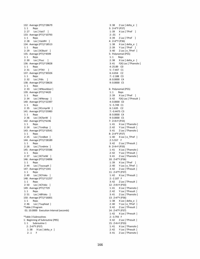
166
132: Average (P71)^28679 1: 1 Reps
2: 27 Loc [ VaisT ] 133: Average (P71)^10793
1: 1 Reps 2: 28 Loc [ VaisRH ] 134: Average (P71)^18513
1: 1 Reps 2: 29 Loc [ DCBusV ] 135: Average (P71)^4599
1: 1 Reps 2: 30 Loc [ Psuc ]
136: Average (P71)^19828 1: 1 Reps 2: 31 Loc [ PTXV ]
137: Average (P71)^30326 1: 1 Reps 2: 32 Loc [ Pdis ]
138: Average (P71)^28626 1: 1 Reps
2: 33 Loc [ WNoutdoor ] 139: Average (P71)^4420 1: 1 Reps
2: 34 Loc [ WNevap ] 140: Average (P71)^22397
1: 1 Reps 2: 35 Loc [ DCcmprW ] 141: Average (P71)^25983
1: 1 Reps 2: 36 Loc [ DCfanW ] 142: Average (P71)^6196
1: 1 Reps 2: 24 Loc [ Tcndtop ]
143: Average (P71)^10541 1: 1 Reps 2: 25 Loc [ Tcndbot ]
144: Average (P71)^28189 1: 1 Reps 2: 26 Loc [ Tcndmix ]
145: Average (P71)^25586 1: 1 Reps
2: 37 Loc [ DCTotW ] 146: Average (P71)^24896 1: 1 Reps
2: 44 Loc [ Tsucsuph ] 147: Average (P71)^1341 1: 1 Reps
2: 49 Loc [ DCYoko ] 148: Average (P71)^11257
1: 1 Reps 2: 50 Loc [ ACYoko ] 149: Average (P71)^729
1: 1 Reps 2: 51 Loc [ ABYoko ]
150: Average (P71)^16001 1: 1 Reps 2: 46 Loc [ Tsupheat ]
*Table 2 Program 01: 10.0000 Execution Interval (seconds)
*Table 3 Subroutines 1: Beginning of Subroutine (P85)
1: 1 Subroutine 1 2: Z=X*F (P37) 1: 38 X Loc [ delta_e ]
2: .1 F
3: 38 Z Loc [ delta_e ] 3: Z=X*F (P37)
1: 39 X Loc [ TPref ] 2: .01 F
3: 39 Z Loc [ TPref ] 4: Z=X*Y (P36) 1: 38 X Loc [ delta_e ]
2: 39 Y Loc [ TPref ] 3: 40 Z Loc [ e_TPref ] 5: Polynomial (P55)
1: 1 Reps 2: 38 X Loc [ delta_e ]
3: 41 F(X) Loc [ TPsensitv ] 4: 25.89 C0 5: -7.447 C1
6: 4.654 C2 7: -2.188 C3 8: 0.0000 C4
9: 0.0000 C5
6: Polynomial (P55) 1: 1 Reps 2: 39 X Loc [ TPref ]
3: 42 F(X) Loc [ TPresult ] 4: 0.0000 C0
5: -5.749 C1 6: 1.635 C2 7: -0.4475 C3
8: 0.0000 C4 9: 0.0000 C5 7: Z=X+Y (P33)
1: 41 X Loc [ TPsensitv ] 2: 42 Y Loc [ TPresult ]
3: 41 Z Loc [ TPsensitv ] 8: Z=X*F (P37) 1: 40 X Loc [ e_TPref ]
2: 5.557 F 3: 42 Z Loc [ TPresult ] 9: Z=X+Y (P33)
1: 41 X Loc [ TPsensitv ] 2: 42 Y Loc [ TPresult ]
3: 41 Z Loc [ TPsensitv ] 10: Z=X*Y (P36) 1: 39 X Loc [ TPref ]
2: 40 Y Loc [ e_TPref ] 3: 42 Z Loc [ TPresult ] 11: Z=X*F (P37)
1: 42 X Loc [ TPresult ] 2: -2.107 F
3: 42 Z Loc [ TPresult ] 12: Z=X+Y (P33) 1: 41 X Loc [ TPsensitv ]
2: 42 Y Loc [ TPresult ] 3: 41 Z Loc [ TPsensitv ]
13: Z=X*Y (P36) 1: 38 X Loc [ delta_e ] 2: 40 Y Loc [ e_TPref ]
3: 42 Z Loc [ TPresult ] 14: Z=X*F (P37) 1: 42 X Loc [ TPresult ]
2: -3.793 F 3: 42 Z Loc [ TPresult ]
15: Z=X+Y (P33) 1: 41 X Loc [ TPsensitv ] 2: 42 Y Loc [ TPresult ]
3: 41 Z Loc [ TPsensitv ]

167
16: Z=X*F (P37) 1: 38 X Loc [ delta_e ]
2: 10 F 3: 38 Z Loc [ delta_e ]
17: Z=X*Y (P36) 1: 41 X Loc [ TPsensitv ] 2: 38 Y Loc [ delta_e ]
3: 42 Z Loc [ TPresult ] 18: Z=X*F (P37) 1: 39 X Loc [ TPref ]
2: 100 F 3: 39 Z Loc [ TPref ]
19: End (P95) ; -------------Type J subroutine----------------
; delta_e is the thermopile voltage difference ; Tref is the reference temperature ; the fit is valid for reference temperatures between 0 and 40
degrees C ; and temperature differences between -40 and +40 C
20: Beginning of Subroutine (P85) 1: 2 Subroutine 2
21: Z=X*F (P37) 1: 38 X Loc [ delta_e ]
2: 0.1 F 3: 47 Z Loc [ del_e_sca ] 22: Polynomial (P55)
1: 1 Reps 2: 47 X Loc [ del_e_sca ] 3: 41 F(X) Loc [ TPsensitv ]
4: 19.7843 C0 5: -2.00106 C1
6: 1.03148 C2 7: -.22977 C3 8: 0.0000 C4
9: 0.0000 C5 23: Z=X*F (P37) 1: 39 X Loc [ TPref ]
2: 0.01 F 3: 48 Z Loc [ Tref_scal ]
24: Polynomial (P55) 1: 1 Reps 2: 48 X Loc [ Tref_scal ]
3: 42 F(X) Loc [ TPresult ] 4: 0 C0 5: -2.02409 C1
6: .698583 C2 7: -.052860 C3
8: 0.0000 C4 9: 0.0000 C5 25: Z=X+Y (P33)
1: 41 X Loc [ TPsensitv ] 2: 42 Y Loc [ TPresult ]
3: 41 Z Loc [ TPsensitv ] 26: Z=X*Y (P36) 1: 38 X Loc [ delta_e ]
2: 39 Y Loc [ TPref ] 3: 40 Z Loc [ e_TPref ] 27: Z=X*F (P37)
1: 40 X Loc [ e_TPref ] 2: .001572 F
3: 42 Z Loc [ TPresult ] 28: Z=X+Y (P33) 1: 41 X Loc [ TPsensitv ]
2: 42 Y Loc [ TPresult ]
3: 41 Z Loc [ TPsensitv ] 29: Z=X*Y (P36)
1: 39 X Loc [ TPref ] 2: 40 Y Loc [ e_TPref ]
3: 42 Z Loc [ TPresult ] 30: Z=X*F (P37) 1: 42 X Loc [ TPresult ]
2: .0001 F 3: 42 Z Loc [ TPresult ] 31: Z=X*F (P37)
1: 42 X Loc [ TPresult ] 2: -.031249 F
3: 42 Z Loc [ TPresult ] 32: Z=X+Y (P33) 1: 41 X Loc [ TPsensitv ]
2: 42 Y Loc [ TPresult ] 3: 41 Z Loc [ TPsensitv ] 33: Z=X*Y (P36)
1: 38 X Loc [ delta_e ] 2: 40 Y Loc [ e_TPref ]
3: 42 Z Loc [ TPresult ] 34: Z=X*F (P37) 1: 42 X Loc [ TPresult ]
2: .0001 F 3: 42 Z Loc [ TPresult ]
35: Z=X*F (P37) 1: 42 X Loc [ TPresult ] 2: -.477042 F
3: 42 Z Loc [ TPresult ] 36: Z=X+Y (P33) 1: 41 X Loc [ TPsensitv ]
2: 42 Y Loc [ TPresult ] 3: 41 Z Loc [ TPsensitv ]
37: Z=X*Y (P36) 1: 41 X Loc [ TPsensitv ] 2: 38 Y Loc [ delta_e ]
3: 42 Z Loc [ TPresult ] 38: End (P95)
End Program

168
A.1.2 Condenser airflow rate measurement
The condenser airflow rate for different condenser fan speeds was measured using an eight
point per radii traverse following the methods described in the section on measuring flow in
ducts in ASHRAE Fundamentals, Chapter 14 Measurement and Instruments [ASHRAE 2001].
The eight sampling points were chosen based on the log-linear rule for circular ducts. A flow
straightener and circular duct was installed on the outlet of the condenser air stream as shown
below. The average of the data from these airflow traverse measurements, along with selected
data recorded using sensors listed in Appendix A.1.1 are shown in the table below.
Condenser airflow rate measurements Fan
Speed
(RPM)
Flow
rate
(CFM)
3-phase
power
(W)
DC
power
(W)
DC bus
voltage
(V)
DC
current
(A)
300 318 1.5 2.5 283 0.009
400 465 3.5 4.6 282 0.016
500 585 6.2 6.9 281 0.025
600 727 10.9 11.6 277 0.042
700 861 16.8 18.1 274 0.066
800 992 24.5 25.9 271 0.096
900 1124 34.0 36.4 267 0.136
1000 1256 46.8 49.4 264 0.187
1100 1392 61.8 66.6 259 0.257

169
A.2 Compressor inverter model
The efficiency of the inverter, or intelligent power module (IPM), providing three phase power
to the compressor is an important consideration in assessing the improved efficiency of the
heat pump or chiller with a variable speed compressor. Significant IPM losses will reduce the
total efficiency of the variable capacity chiller or heat pump relative to a constant speed system
operating at the same frequency. A model of the IPM losses is shown below. The IPM converts
direct current (DC) power into three-phase alternating-current (AC) power at different
frequencies to drive the compressor. The power losses at the IPM depend strongly on the total
three phase power consumption of the compressor, and have a weaker dependence on the
compressor speed.
15 20 25 30 35 40 45 50 55 6015
20
25
30
35
40
45
50
55
60
RMSE = 2.6 W
Relative RMSE = 9.5 %IPM Loss (W) = 24 + 0.046W
3φcomp - 0.24ωcomp - 0.0026ωcomp
2 +/- 2.6 W
Measured IPM loss (W)
Modeled IPM Loss (W)
Modeled compressor inverter (IPM) losses

170
A.3 Low lift heat pump performance data
Test conditions Refrigerant Temperatures Refrigerant pressures
Test
point
Comp-
ressor
Speed
(Hz)
Condenser
fan speed
(RPM)
Zone
Air
Temp
(C)
Outdoor
Air
Temp
(C)
Suction
Temp
(C)
Discharge
Temp (C)
Condenser
Outlet
Temp (C)
EXV
Outlet
Temp
(C)
Evaporator
Inlet
Temp (C)
Ambient
Pressure
(kPa)
Suction
pressure
(psig)
Post-
EXV
pressure
(psig)
Discharge
pressure
(psig)
1 19 750 23.93 22.75 15.65 39.42 24.36 15.13 15.01 102.91 164 166 248
2 60 750 23.96 22.61 4.67 56.94 25.54 7.18 6.80 101.66 112 125 300
3 30 750 23.85 22.32 12.06 44.95 26.22 12.03 11.81 102.47 145 150 260
4 60 750 34.07 22.55 10.36 57.85 26.79 12.71 12.31 101.59 137 152 319
5 30 750 34.14 22.76 22.60 47.40 24.85 18.12 18.00 102.74 178 183 272
6 19 750 33.93 30.22 24.83 46.90 32.69 23.41 23.26 101.52 211 214 306
7 30 750 34.22 30.40 20.81 50.00 34.68 21.22 21.01 101.76 194 200 327
8 19 750 34.07 37.47 25.11 54.48 40.42 25.14 24.91 102.44 220 224 364
9 30 750 33.98 37.73 21.84 59.33 41.37 22.38 22.16 101.66 199 206 384
10 30 750 34.16 45.10 23.48 69.24 50.11 24.29 23.89 101.52 208 217 454
11 30 750 14.85 18.09 4.79 36.85 20.67 5.03 4.85 101.49 114 117 217
12 60 750 24.11 18.76 6.70 56.21 22.26 5.45 5.07 101.59 105 118 263
13 60 750 33.93 18.54 14.92 59.72 21.42 10.62 10.26 101.56 130 142 288
14 19 750 14.12 16.70 8.33 35.02 17.19 6.71 6.59 101.22 123 125 200
15 30 750 14.03 16.57 4.42 36.31 18.55 4.53 4.38 101.22 112 115 208
16 60 750 23.84 17.71 7.51 56.97 20.79 4.95 4.60 101.42 104 116 256
17 30 750 24.01 16.63 15.46 44.48 17.41 9.68 9.51 101.19 135 138 223
18 19 750 13.98 15.42 7.99 33.28 16.30 5.95 5.86 102.44 120 121 192
19 19 750 13.89 15.42 7.90 33.25 16.33 5.91 5.81 102.44 120 121 191
20 19 750 13.93 15.46 7.95 33.22 16.41 5.93 5.83 102.44 120 121 191
21 95 750 14.12 16.28 -1.16 84.57 17.85 -3.19 -3.83 102.44 64 82 284
22 95 750 24.09 16.73 4.28 81.36 19.35 2.47 1.91 102.44 82 104 306
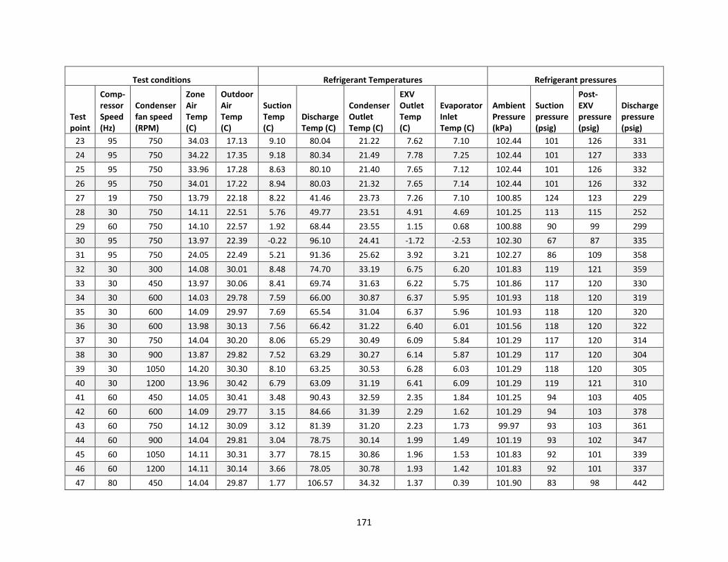
171
Test conditions Refrigerant Temperatures Refrigerant pressures
Test
point
Comp-
ressor
Speed
(Hz)
Condenser
fan speed
(RPM)
Zone
Air
Temp
(C)
Outdoor
Air
Temp
(C)
Suction
Temp
(C)
Discharge
Temp (C)
Condenser
Outlet
Temp (C)
EXV
Outlet
Temp
(C)
Evaporator
Inlet
Temp (C)
Ambient
Pressure
(kPa)
Suction
pressure
(psig)
Post-
EXV
pressure
(psig)
Discharge
pressure
(psig)
23 95 750 34.03 17.13 9.10 80.04 21.22 7.62 7.10 102.44 101 126 331
24 95 750 34.22 17.35 9.18 80.34 21.49 7.78 7.25 102.44 101 127 333
25 95 750 33.96 17.28 8.63 80.10 21.40 7.65 7.12 102.44 101 126 332
26 95 750 34.01 17.22 8.94 80.03 21.32 7.65 7.14 102.44 101 126 332
27 19 750 13.79 22.18 8.22 41.46 23.73 7.26 7.10 100.85 124 123 229
28 30 750 14.11 22.51 5.76 49.77 23.51 4.91 4.69 101.25 113 115 252
29 60 750 14.10 22.57 1.92 68.44 23.55 1.15 0.68 100.88 90 99 299
30 95 750 13.97 22.39 -0.22 96.10 24.41 -1.72 -2.53 102.30 67 87 335
31 95 750 24.05 22.49 5.21 91.36 25.62 3.92 3.21 102.27 86 109 358
32 30 300 14.08 30.01 8.48 74.70 33.19 6.75 6.20 101.83 119 121 359
33 30 450 13.97 30.06 8.41 69.74 31.63 6.22 5.75 101.86 117 120 330
34 30 600 14.03 29.78 7.59 66.00 30.87 6.37 5.95 101.93 118 120 319
35 30 600 14.09 29.97 7.69 65.54 31.04 6.37 5.96 101.93 118 120 320
36 30 600 13.98 30.13 7.56 66.42 31.22 6.40 6.01 101.56 118 120 322
37 30 750 14.04 30.20 8.06 65.29 30.49 6.09 5.84 101.29 117 120 314
38 30 900 13.87 29.82 7.52 63.29 30.27 6.14 5.87 101.29 117 120 304
39 30 1050 14.20 30.30 8.10 63.25 30.53 6.28 6.03 101.29 118 120 305
40 30 1200 13.96 30.42 6.79 63.09 31.19 6.41 6.09 101.29 119 121 310
41 60 450 14.05 30.41 3.48 90.43 32.59 2.35 1.84 101.25 94 103 405
42 60 600 14.09 29.77 3.15 84.66 31.39 2.29 1.62 101.29 94 103 378
43 60 750 14.12 30.09 3.12 81.39 31.20 2.23 1.73 99.97 93 103 361
44 60 900 14.04 29.81 3.04 78.75 30.14 1.99 1.49 101.19 93 102 347
45 60 1050 14.11 30.31 3.77 78.15 30.86 1.96 1.53 101.83 92 101 339
46 60 1200 14.11 30.14 3.66 78.05 30.78 1.93 1.42 101.83 92 101 337
47 80 450 14.04 29.87 1.77 106.57 34.32 1.37 0.39 101.90 83 98 442

172
Test conditions Refrigerant Temperatures Refrigerant pressures
Test
point
Comp-
ressor
Speed
(Hz)
Condenser
fan speed
(RPM)
Zone
Air
Temp
(C)
Outdoor
Air
Temp
(C)
Suction
Temp
(C)
Discharge
Temp (C)
Condenser
Outlet
Temp (C)
EXV
Outlet
Temp
(C)
Evaporator
Inlet
Temp (C)
Ambient
Pressure
(kPa)
Suction
pressure
(psig)
Post-
EXV
pressure
(psig)
Discharge
pressure
(psig)
48 89 600 13.97 29.76 0.99 108.13 33.14 0.43 -0.52 101.90 76 95 422
49 93 750 14.08 30.20 0.13 106.92 33.06 0.40 -0.59 101.90 75 94 412
50 93 900 13.96 30.11 0.45 104.71 32.37 0.12 -0.83 101.86 74 93 395
51 93 1050 14.01 30.21 0.98 103.98 32.05 -0.12 -1.03 101.86 73 93 385
52 93 1200 13.93 29.97 1.16 103.33 31.44 -0.51 -1.33 101.83 72 91 375
53 19 300 23.97 30.23 18.13 59.26 34.22 16.62 16.38 101.69 170 172 336
54 19 450 24.05 30.16 18.00 54.43 32.20 16.29 16.16 101.69 169 170 314
55 19 600 23.94 30.29 17.88 53.64 31.98 16.16 16.00 101.69 168 170 308
56 19 750 24.15 30.26 18.15 52.15 31.58 16.22 16.07 101.76 168 170 301
57 19 900 24.04 30.22 18.09 51.62 31.32 16.05 15.88 101.76 168 169 297
58 19 1050 24.01 30.06 18.32 51.49 30.96 15.87 15.72 101.83 167 168 294
59 19 1200 24.01 29.98 17.65 49.47 31.06 16.10 15.92 101.86 168 170 291
60 30 1050 14.14 30.03 8.30 63.21 30.44 6.09 5.82 102.10 117 119 301
61 30 1200 14.07 30.16 8.29 63.21 30.48 6.05 5.79 102.10 117 119 301
62 60 450 24.02 29.90 10.00 85.97 35.75 9.14 8.48 101.42 120 132 432
63 60 600 23.98 29.78 9.56 77.35 34.55 8.78 8.10 101.32 119 131 381
64 60 750 24.07 30.07 9.45 74.76 33.73 8.68 8.07 101.49 118 131 368
65 60 900 24.19 29.93 9.62 72.82 32.44 8.34 7.81 101.52 117 129 352
66 60 1050 23.98 30.22 9.39 71.93 32.36 8.31 7.77 101.59 117 129 348
67 60 1200 24.00 29.81 10.00 71.16 31.43 7.68 7.09 101.35 114 126 335
68 84 450 24.00 29.83 7.98 107.08 36.51 6.58 5.67 102.64 101 120 480
69 88 600 24.07 29.57 7.36 103.15 33.53 5.55 4.75 102.68 95 115 438
70 93 750 23.92 30.30 6.40 102.38 32.92 5.30 4.53 102.68 91 115 423
71 95 900 23.99 30.01 5.35 100.00 32.27 5.05 4.21 102.74 89 113 408
72 95 1050 24.05 29.87 6.04 98.98 31.63 4.96 4.05 102.74 89 113 397

173
Test conditions Refrigerant Temperatures Refrigerant pressures
Test
point
Comp-
ressor
Speed
(Hz)
Condenser
fan speed
(RPM)
Zone
Air
Temp
(C)
Outdoor
Air
Temp
(C)
Suction
Temp
(C)
Discharge
Temp (C)
Condenser
Outlet
Temp (C)
EXV
Outlet
Temp
(C)
Evaporator
Inlet
Temp (C)
Ambient
Pressure
(kPa)
Suction
pressure
(psig)
Post-
EXV
pressure
(psig)
Discharge
pressure
(psig)
73 95 1200 23.98 30.01 5.45 96.77 30.90 4.86 4.03 102.74 88 112 387
74 60 750 34.03 30.04 16.25 74.97 33.81 13.96 13.44 102.61 142 156 389
75 89 750 34.23 30.14 13.75 98.08 34.71 10.99 10.15 102.64 115 140 443
76 50 750 26.79 35.30 13.56 75.34 38.23 13.16 12.59 101.96 142 152 403
77 50 750 26.94 35.20 14.09 75.35 38.70 13.23 12.54 101.96 142 153 399
78 30 750 14.03 37.33 9.51 78.90 38.03 6.94 6.51 102.00 119 123 371
79 60 750 13.98 37.93 4.55 94.57 39.66 3.83 2.98 101.19 97 108 434
80 79 750 14.05 37.51 3.29 110.48 39.44 1.60 0.70 100.88 84 99 456
81 60 750 24.06 37.21 11.43 88.13 38.93 9.28 8.58 100.78 120 132 431
82 95 750 24.10 37.21 8.03 104.65 40.61 7.82 6.77 102.61 104 125 476
83 60 750 33.91 37.45 16.28 84.34 42.53 16.09 15.14 102.64 151 167 463
84 81 750 34.00 37.27 14.10 98.08 42.63 13.84 12.92 102.44 131 154 495
85 30 750 14.11 45.02 10.15 90.48 45.58 8.42 7.89 102.51 125 128 443
86 30 900 14.11 45.05 9.79 90.18 45.45 8.49 7.98 102.51 125 129 437
87 30 1050 13.92 45.19 9.91 90.93 45.69 8.45 7.77 102.51 125 128 437
88 30 1200 14.21 45.25 10.64 90.57 45.62 8.39 7.72 102.51 125 128 435
89 60 600 14.07 44.77 6.10 110.83 46.82 5.20 4.38 102.47 102 113 522
90 60 750 14.15 45.06 5.93 106.91 46.69 5.46 4.51 102.44 102 114 507
91 60 900 13.99 45.10 5.83 105.80 46.40 5.27 4.27 102.47 101 113 497
92 60 1050 14.04 44.95 5.63 103.87 46.02 5.29 4.32 102.47 102 113 488
93 60 1200 14.09 44.94 5.59 102.66 46.06 5.36 4.27 102.51 102 113 485
94 68 900 14.04 45.10 5.16 111.75 46.64 4.41 3.37 101.52 96 110 509
95 68 1050 13.85 45.10 5.17 111.10 46.24 4.08 3.03 101.52 95 108 500
96 68 1200 14.13 45.16 5.71 110.76 46.01 3.99 3.03 101.52 94 108 493
97 30 750 23.98 45.37 17.99 83.64 46.71 15.97 15.50 102.64 162 166 457

174
Test conditions Refrigerant Temperatures Refrigerant pressures
Test
point
Comp-
ressor
Speed
(Hz)
Condenser
fan speed
(RPM)
Zone
Air
Temp
(C)
Outdoor
Air
Temp
(C)
Suction
Temp
(C)
Discharge
Temp (C)
Condenser
Outlet
Temp (C)
EXV
Outlet
Temp
(C)
Evaporator
Inlet
Temp (C)
Ambient
Pressure
(kPa)
Suction
pressure
(psig)
Post-
EXV
pressure
(psig)
Discharge
pressure
(psig)
98 30 750 24.02 45.37 17.32 82.27 46.86 16.28 15.81 102.64 163 168 457
99 60 750 23.93 45.01 12.00 99.48 48.02 11.77 10.86 102.61 129 144 523
100 75 750 24.16 45.18 11.43 111.20 48.45 10.60 9.57 102.64 118 137 548
101 19 750 34.05 45.07 28.03 69.80 46.97 26.06 25.73 102.03 225 228 436
102 74 750 33.92 44.54 15.86 102.25 49.16 16.21 15.17 102.44 144 166 548
103 19 750 14.02 14.76 7.67 32.71 15.42 6.09 6.02 99.32 122 122 190
104 30 750 13.89 17.60 5.61 43.07 18.56 3.92 3.74 101.90 110 111 216
105 60 750 13.86 19.21 1.17 63.96 20.02 -0.46 -0.88 101.86 85 93 265
106 95 750 13.96 19.10 -1.44 92.37 20.62 -3.81 -4.55 100.78 62 80 306
107 19 750 24.10 17.11 16.51 31.97 19.31 13.68 13.63 101.86 158 160 207
108 30 750 23.86 17.26 13.10 40.90 18.20 10.40 10.27 101.90 139 142 225
109 60 750 24.06 17.84 7.40 60.26 19.72 4.66 4.32 100.85 104 114 270
110 95 750 24.61 19.14 4.19 87.60 21.63 2.02 1.38 100.81 80 102 326
111 30 750 34.02 17.98 20.12 39.22 20.20 16.81 16.73 101.86 173 177 238
112 60 750 34.22 17.28 12.85 56.52 20.32 10.01 9.75 100.85 128 139 278
113 19 750 24.05 22.80 16.08 38.45 23.57 14.60 14.50 103.08 162 163 239
114 30 750 24.03 22.68 14.01 49.19 23.93 11.57 11.38 100.95 144 147 265
115 60 750 24.28 23.09 8.61 69.42 25.39 5.76 5.22 100.95 108 118 315
116 19 750 34.01 22.68 23.70 36.81 26.82 21.83 21.73 100.24 204 206 253
117 30 750 34.13 22.62 20.55 45.41 25.62 18.31 18.11 101.15 180 184 274
118 30 300 23.93 29.84 14.83 69.09 35.49 13.93 13.51 102.47 153 157 377
119 30 450 24.06 30.01 15.56 64.55 32.63 13.13 12.73 102.44 149 153 341
120 30 600 23.78 30.10 14.78 61.86 32.29 13.13 12.77 102.47 150 153 331
121 30 750 24.07 30.26 15.29 62.30 32.38 13.24 12.91 102.54 150 153 332
122 30 900 23.93 30.46 14.64 60.26 32.39 13.36 13.02 102.98 151 154 326

175
Test conditions Refrigerant Temperatures Refrigerant pressures
Test
point
Comp-
ressor
Speed
(Hz)
Condenser
fan speed
(RPM)
Zone
Air
Temp
(C)
Outdoor
Air
Temp
(C)
Suction
Temp
(C)
Discharge
Temp (C)
Condenser
Outlet
Temp (C)
EXV
Outlet
Temp
(C)
Evaporator
Inlet
Temp (C)
Ambient
Pressure
(kPa)
Suction
pressure
(psig)
Post-
EXV
pressure
(psig)
Discharge
pressure
(psig)
123 19 750 34.04 29.93 25.09 47.89 32.15 22.82 22.69 99.93 207 210 304
124 30 750 34.16 29.79 22.05 55.78 32.60 19.37 19.11 99.90 184 188 324
125 19 750 24.01 37.60 18.57 64.23 38.38 16.74 16.43 100.10 170 172 359
126 30 750 23.98 37.54 15.76 70.97 38.84 14.32 13.83 101.08 155 158 382
127 19 750 34.02 37.41 25.81 57.10 41.01 24.43 24.09 100.07 216 219 363
128 30 750 34.19 37.57 23.65 68.25 39.92 20.88 20.48 101.05 191 195 395
129 30 750 33.77 45.15 23.96 76.81 47.93 22.80 22.19 101.12 200 206 464
130 60 750 33.59 44.85 17.87 98.30 48.24 16.22 15.24 101.15 150 166 532
131 19 750 24.13 30.08 17.59 51.98 31.69 16.09 15.75 103.01 168 169 301
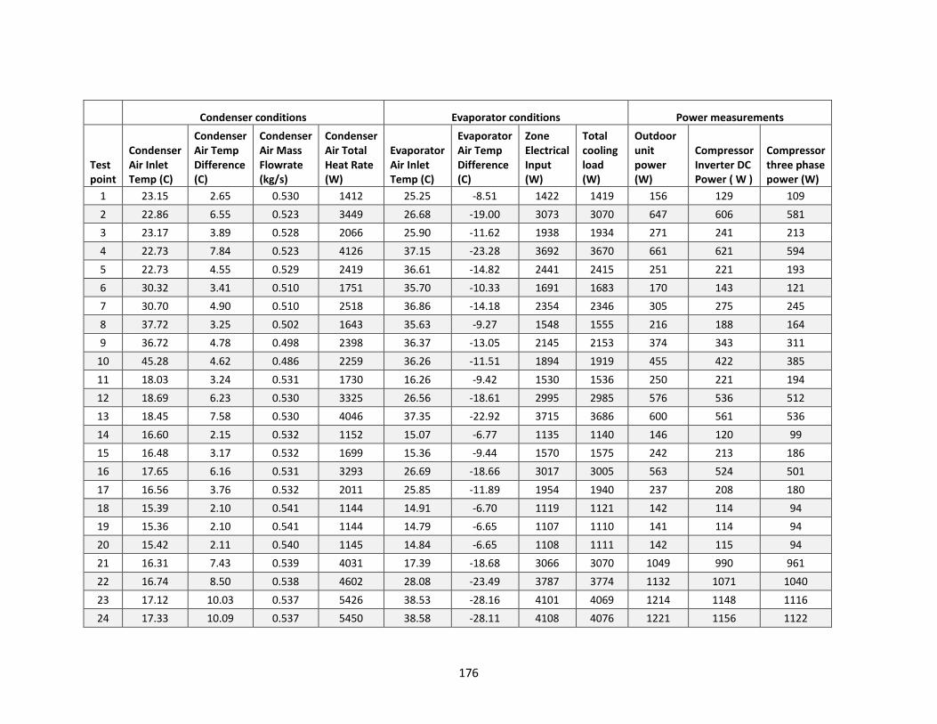
176
Condenser conditions Evaporator conditions Power measurements
Test
point
Condenser
Air Inlet
Temp (C)
Condenser
Air Temp
Difference
(C)
Condenser
Air Mass
Flowrate
(kg/s)
Condenser
Air Total
Heat Rate
(W)
Evaporator
Air Inlet
Temp (C)
Evaporator
Air Temp
Difference
(C)
Zone
Electrical
Input
(W)
Total
cooling
load
(W)
Outdoor
unit
power
(W)
Compressor
Inverter DC
Power ( W )
Compressor
three phase
power (W)
1 23.15 2.65 0.530 1412 25.25 -8.51 1422 1419 156 129 109
2 22.86 6.55 0.523 3449 26.68 -19.00 3073 3070 647 606 581
3 23.17 3.89 0.528 2066 25.90 -11.62 1938 1934 271 241 213
4 22.73 7.84 0.523 4126 37.15 -23.28 3692 3670 661 621 594
5 22.73 4.55 0.529 2419 36.61 -14.82 2441 2415 251 221 193
6 30.32 3.41 0.510 1751 35.70 -10.33 1691 1683 170 143 121
7 30.70 4.90 0.510 2518 36.86 -14.18 2354 2346 305 275 245
8 37.72 3.25 0.502 1643 35.63 -9.27 1548 1555 216 188 164
9 36.72 4.78 0.498 2398 36.37 -13.05 2145 2153 374 343 311
10 45.28 4.62 0.486 2259 36.26 -11.51 1894 1919 455 422 385
11 18.03 3.24 0.531 1730 16.26 -9.42 1530 1536 250 221 194
12 18.69 6.23 0.530 3325 26.56 -18.61 2995 2985 576 536 512
13 18.45 7.58 0.530 4046 37.35 -22.92 3715 3686 600 561 536
14 16.60 2.15 0.532 1152 15.07 -6.77 1135 1140 146 120 99
15 16.48 3.17 0.532 1699 15.36 -9.44 1570 1575 242 213 186
16 17.65 6.16 0.531 3293 26.69 -18.66 3017 3005 563 524 501
17 16.56 3.76 0.532 2011 25.85 -11.89 1954 1940 237 208 180
18 15.39 2.10 0.541 1144 14.91 -6.70 1119 1121 142 114 94
19 15.36 2.10 0.541 1144 14.79 -6.65 1107 1110 141 114 94
20 15.42 2.11 0.540 1145 14.84 -6.65 1108 1111 142 115 94
21 16.31 7.43 0.539 4031 17.39 -18.68 3066 3070 1049 990 961
22 16.74 8.50 0.538 4602 28.08 -23.49 3787 3774 1132 1071 1040
23 17.12 10.03 0.537 5426 38.53 -28.16 4101 4069 1214 1148 1116
24 17.33 10.09 0.537 5450 38.58 -28.11 4108 4076 1221 1156 1122

177
Condenser conditions Evaporator conditions Power measurements
Test
point
Condenser
Air Inlet
Temp (C)
Condenser
Air Temp
Difference
(C)
Condenser
Air Mass
Flowrate
(kg/s)
Condenser
Air Total
Heat Rate
(W)
Evaporator
Air Inlet
Temp (C)
Evaporator
Air Temp
Difference
(C)
Zone
Electrical
Input
(W)
Total
cooling
load
(W)
Outdoor
unit
power
(W)
Compressor
Inverter DC
Power ( W )
Compressor
three phase
power (W)
25 17.26 10.07 0.537 5441 38.13 -27.88 4078 4048 1218 1152 1119
26 17.20 10.03 0.537 5422 38.51 -28.15 4101 4070 1217 1151 1118
27 24.26 2.07 0.520 1085 14.87 -6.16 1012 1027 168 142 121
28 22.71 3.14 0.521 1646 15.57 -8.89 1471 1486 288 258 230
29 22.42 5.93 0.519 3101 17.04 -15.25 2463 2479 654 613 588
30 22.65 7.39 0.527 3919 17.04 -17.36 2886 2901 1179 1119 1085
31 22.78 8.76 0.527 4643 27.95 -22.16 3657 3654 1273 1208 1173
32 30.00 8.53 0.189 1625 15.44 -7.82 1285 1313 372 359 326
33 30.22 5.27 0.294 1559 15.37 -8.02 1315 1344 348 332 302
34 30.34 3.82 0.402 1548 15.46 -8.22 1343 1371 343 322 291
35 30.46 3.82 0.402 1546 15.57 -8.22 1349 1378 344 322 292
36 30.40 3.83 0.400 1542 15.36 -8.10 1333 1362 346 324 293
37 30.70 3.02 0.508 1546 15.43 -8.14 1343 1372 347 304 273
38 29.95 2.59 0.620 1615 15.22 -8.14 1345 1374 351 307 277
39 30.27 2.28 0.732 1677 15.57 -8.18 1360 1389 373 307 277
40 30.93 1.96 0.846 1672 15.30 -8.12 1346 1375 405 313 283
41 30.56 9.86 0.292 2896 16.56 -13.62 2202 2231 822 791 756
42 30.53 6.96 0.400 2799 16.75 -13.95 2253 2281 783 748 715
43 30.20 6.04 0.502 3051 16.74 -14.23 2267 2295 763 719 688
44 30.09 4.63 0.620 2889 16.72 -14.17 2304 2333 752 691 665
45 29.77 3.95 0.736 2926 16.65 -14.12 2277 2306 757 681 649
46 30.06 3.46 0.851 2964 16.64 -14.12 2272 2301 782 678 647
47 30.08 12.65 0.294 3746 16.92 -15.71 2507 2535 1197 1152 1111
48 29.93 9.84 0.402 3984 17.08 -16.60 2654 2682 1313 1256 1217
49 30.00 7.76 0.511 3995 17.25 -17.03 2728 2757 1359 1293 1255

178
Condenser conditions Evaporator conditions Power measurements
Test
point
Condenser
Air Inlet
Temp (C)
Condenser
Air Temp
Difference
(C)
Condenser
Air Mass
Flowrate
(kg/s)
Condenser
Air Total
Heat Rate
(W)
Evaporator
Air Inlet
Temp (C)
Evaporator
Air Temp
Difference
(C)
Zone
Electrical
Input
(W)
Total
cooling
load
(W)
Outdoor
unit
power
(W)
Compressor
Inverter DC
Power ( W )
Compressor
three phase
power (W)
50 30.13 6.30 0.623 3952 17.22 -17.07 2738 2767 1332 1252 1215
51 30.20 5.35 0.736 3963 17.24 -17.01 2727 2757 1327 1227 1191
52 30.00 4.64 0.852 3977 17.14 -16.89 2713 2742 1327 1201 1165
53 30.03 7.54 0.189 1435 25.15 -7.31 1209 1220 208 200 171
54 30.14 4.60 0.293 1357 25.28 -7.66 1260 1271 192 181 155
55 30.07 3.34 0.401 1347 25.17 -7.68 1256 1268 193 176 151
56 29.86 2.61 0.511 1340 25.46 -7.79 1281 1292 198 171 146
57 29.85 2.16 0.622 1354 25.34 -7.80 1279 1290 209 167 143
58 29.98 1.81 0.737 1341 25.30 -7.75 1279 1290 227 166 142
59 30.12 1.60 0.852 1372 25.33 -7.83 1300 1311 251 163 138
60 29.65 2.24 0.739 1668 15.53 -8.21 1350 1379 369 305 274
61 30.04 1.94 0.853 1666 15.47 -8.21 1346 1375 396 305 273
62 30.39 11.84 0.293 3491 26.91 -17.14 2867 2877 788 840 802
63 30.24 8.45 0.400 3400 26.95 -17.59 2885 2895 771 752 718
64 30.58 6.55 0.510 3363 27.03 -17.72 2885 2896 771 728 695
65 30.11 5.36 0.622 3354 27.08 -17.91 2885 2895 771 701 669
66 30.61 4.58 0.734 3387 26.98 -17.90 2885 2896 771 692 661
67 29.72 3.88 0.848 3308 26.93 -17.87 2777 2788 873 669 638
68 30.48 15.26 0.296 4555 26.96 -19.77 3164 3175 1407 1352 1306
69 29.95 11.06 0.405 4513 27.12 -20.63 3288 3298 1380 1319 1277
70 30.62 8.58 0.515 4453 27.06 -20.85 3334 3345 1426 1353 1313
71 30.32 7.07 0.629 4475 27.10 -21.04 3381 3392 1427 1342 1303
72 30.01 6.07 0.744 4545 27.33 -21.21 3392 3402 1417 1312 1274
73 29.86 5.23 0.859 4521 27.18 -21.28 3418 3429 1417 1285 1248
74 30.11 7.89 0.515 4093 37.24 -21.60 3504 3497 804 758 724
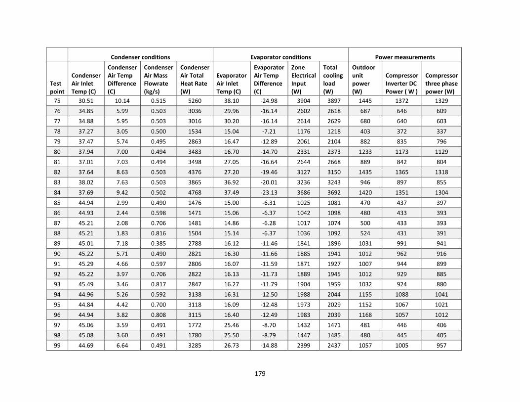
179
Condenser conditions Evaporator conditions Power measurements
Test
point
Condenser
Air Inlet
Temp (C)
Condenser
Air Temp
Difference
(C)
Condenser
Air Mass
Flowrate
(kg/s)
Condenser
Air Total
Heat Rate
(W)
Evaporator
Air Inlet
Temp (C)
Evaporator
Air Temp
Difference
(C)
Zone
Electrical
Input
(W)
Total
cooling
load
(W)
Outdoor
unit
power
(W)
Compressor
Inverter DC
Power ( W )
Compressor
three phase
power (W)
75 30.51 10.14 0.515 5260 38.10 -24.98 3904 3897 1445 1372 1329
76 34.85 5.99 0.503 3036 29.96 -16.14 2602 2618 687 646 609
77 34.88 5.95 0.503 3016 30.20 -16.14 2614 2629 680 640 603
78 37.27 3.05 0.500 1534 15.04 -7.21 1176 1218 403 372 337
79 37.47 5.74 0.495 2863 16.47 -12.89 2061 2104 882 835 796
80 37.94 7.00 0.494 3483 16.70 -14.70 2331 2373 1233 1173 1129
81 37.01 7.03 0.494 3498 27.05 -16.64 2644 2668 889 842 804
82 37.64 8.63 0.503 4376 27.20 -19.46 3127 3150 1435 1365 1318
83 38.02 7.63 0.503 3865 36.92 -20.01 3236 3243 946 897 855
84 37.69 9.42 0.502 4768 37.49 -23.13 3686 3692 1420 1351 1304
85 44.94 2.99 0.490 1476 15.00 -6.31 1025 1081 470 437 397
86 44.93 2.44 0.598 1471 15.06 -6.37 1042 1098 480 433 393
87 45.21 2.08 0.706 1481 14.86 -6.28 1017 1074 500 433 393
88 45.21 1.83 0.816 1504 15.14 -6.37 1036 1092 524 431 391
89 45.01 7.18 0.385 2788 16.12 -11.46 1841 1896 1031 991 941
90 45.22 5.71 0.490 2821 16.30 -11.66 1885 1941 1012 962 916
91 45.29 4.66 0.597 2806 16.07 -11.59 1871 1927 1007 944 899
92 45.22 3.97 0.706 2822 16.13 -11.73 1889 1945 1012 929 885
93 45.49 3.46 0.817 2847 16.27 -11.79 1904 1959 1032 924 880
94 44.96 5.26 0.592 3138 16.31 -12.50 1988 2044 1155 1088 1041
95 44.84 4.42 0.700 3118 16.09 -12.48 1973 2029 1152 1067 1021
96 44.94 3.82 0.808 3115 16.40 -12.49 1983 2039 1168 1057 1012
97 45.06 3.59 0.491 1772 25.46 -8.70 1432 1471 481 446 406
98 45.08 3.60 0.491 1780 25.50 -8.79 1447 1485 480 445 405
99 44.69 6.64 0.491 3285 26.73 -14.88 2399 2437 1057 1005 957

180
Condenser conditions Evaporator conditions Power measurements
Test
point
Condenser
Air Inlet
Temp (C)
Condenser
Air Temp
Difference
(C)
Condenser
Air Mass
Flowrate
(kg/s)
Condenser
Air Total
Heat Rate
(W)
Evaporator
Air Inlet
Temp (C)
Evaporator
Air Temp
Difference
(C)
Zone
Electrical
Input
(W)
Total
cooling
load
(W)
Outdoor
unit
power
(W)
Compressor
Inverter DC
Power ( W )
Compressor
three phase
power (W)
100 44.88 8.07 0.491 3990 27.31 -16.94 2717 2755 1419 1353 1300
101 45.07 3.07 0.488 1509 35.58 -8.19 1355 1375 279 252 218
102 44.70 9.17 0.491 4535 36.93 -20.63 3284 3303 1415 1346 1294
103 14.83 2.09 0.525 1106 14.58 -6.89 1131 1132 148 114 95
104 17.58 2.94 0.534 1578 14.67 -9.18 1543 1550 322 224 197
105 19.15 5.48 0.531 2928 15.19 -14.72 2411 2421 624 555 531
106 19.10 7.39 0.525 3906 15.18 -17.71 2834 2843 1181 1040 1008
107 17.11 2.66 0.534 1433 24.79 -8.79 1476 1464 164 98 79
108 17.26 3.75 0.534 2015 25.08 -12.19 2038 2026 325 208 180
109 17.80 6.76 0.528 3587 25.41 -18.78 3008 2997 643 552 528
110 19.18 8.72 0.525 4610 26.26 -22.54 3614 3604 1280 1127 1095
111 18.04 4.65 0.533 2495 35.50 -15.30 2549 2521 271 185 157
112 17.24 7.80 0.529 4149 36.02 -23.40 3732 3702 633 542 518
113 21.84 2.87 0.530 1530 24.81 -8.46 1418 1415 157 124 103
114 22.47 4.24 0.520 2217 25.14 -11.52 1905 1903 286 249 221
115 23.30 6.99 0.519 3650 25.61 -18.02 2910 2908 715 638 610
116 22.81 3.86 0.516 2004 35.09 -10.98 1807 1786 132 101 80
117 22.97 5.04 0.521 2642 35.53 -14.81 2444 2424 261 225 196
118 30.16 10.52 0.191 2018 24.89 -10.00 1686 1696 386 367 334
119 30.04 6.39 0.296 1901 25.08 -10.28 1733 1744 352 331 299
120 30.56 4.77 0.404 1938 24.80 -10.43 1744 1755 346 320 289
121 31.45 3.62 0.515 1874 25.10 -10.43 1750 1761 357 320 290
122 31.60 3.02 0.629 1910 24.95 -10.44 1756 1767 364 314 284
123 30.18 3.36 0.502 1699 34.90 -10.10 1659 1652 175 144 123
124 30.11 4.65 0.502 2351 35.47 -13.89 2241 2233 318 283 253

181
Condenser conditions Evaporator conditions Power measurements
Test
point
Condenser
Air Inlet
Temp (C)
Condenser
Air Temp
Difference
(C)
Condenser
Air Mass
Flowrate
(kg/s)
Condenser
Air Total
Heat Rate
(W)
Evaporator
Air Inlet
Temp (C)
Evaporator
Air Temp
Difference
(C)
Zone
Electrical
Input
(W)
Total
cooling
load
(W)
Outdoor
unit
power
(W)
Compressor
Inverter DC
Power ( W )
Compressor
three phase
power (W)
125 37.59 2.47 0.490 1220 24.56 -6.81 1098 1122 249 216 188
126 37.62 3.63 0.495 1812 24.92 -9.78 1603 1627 410 373 340
127 37.52 3.31 0.491 1633 34.88 -9.15 1479 1485 222 190 164
128 37.48 4.47 0.495 2227 35.49 -12.67 2081 2087 402 366 332
129 45.33 4.43 0.484 2161 34.96 -11.58 1876 1897 479 439 400
130 44.89 7.68 0.484 3746 35.12 -17.91 2838 2858 1093 1036 989
131 30.49 2.53 0.517 1319 24.82 -7.46 1269 1280 204 172 148
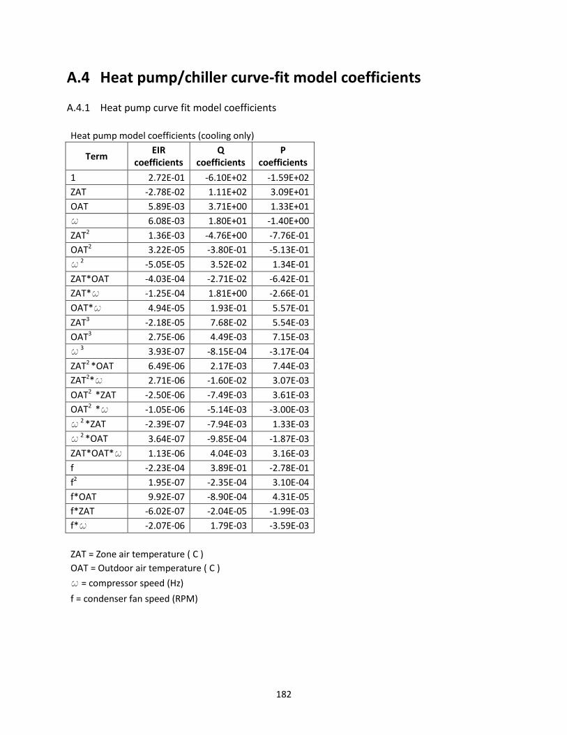
182
A.4 Heat pump/chiller curve-fit model coefficients
A.4.1 Heat pump curve fit model coefficients
Heat pump model coefficients (cooling only)
Term EIR
coefficients
Q
coefficients
P
coefficients
1 2.72E-01 -6.10E+02 -1.59E+02
ZAT -2.78E-02 1.11E+02 3.09E+01
OAT 5.89E-03 3.71E+00 1.33E+01
w 6.08E-03 1.80E+01 -1.40E+00
ZAT2 1.36E-03 -4.76E+00 -7.76E-01
OAT2 3.22E-05 -3.80E-01 -5.13E-01
w 2 -5.05E-05 3.52E-02 1.34E-01
ZAT*OAT -4.03E-04 -2.71E-02 -6.42E-01
ZAT*w -1.25E-04 1.81E+00 -2.66E-01
OAT*w 4.94E-05 1.93E-01 5.57E-01
ZAT3 -2.18E-05 7.68E-02 5.54E-03
OAT3 2.75E-06 4.49E-03 7.15E-03
w 3 3.93E-07 -8.15E-04 -3.17E-04
ZAT2 *OAT 6.49E-06 2.17E-03 7.44E-03
ZAT2*w 2.71E-06 -1.60E-02 3.07E-03
OAT2 *ZAT -2.50E-06 -7.49E-03 3.61E-03
OAT2 *w -1.05E-06 -5.14E-03 -3.00E-03
w 2 *ZAT -2.39E-07 -7.94E-03 1.33E-03
w 2 *OAT 3.64E-07 -9.85E-04 -1.87E-03
ZAT*OAT*w 1.13E-06 4.04E-03 3.16E-03
f -2.23E-04 3.89E-01 -2.78E-01
f2 1.95E-07 -2.35E-04 3.10E-04
f*OAT 9.92E-07 -8.90E-04 4.31E-05
f*ZAT -6.02E-07 -2.04E-05 -1.99E-03
f*w -2.07E-06 1.79E-03 -3.59E-03
ZAT = Zone air temperature ( C )
OAT = Outdoor air temperature ( C )
w = compressor speed (Hz)
f = condenser fan speed (RPM)
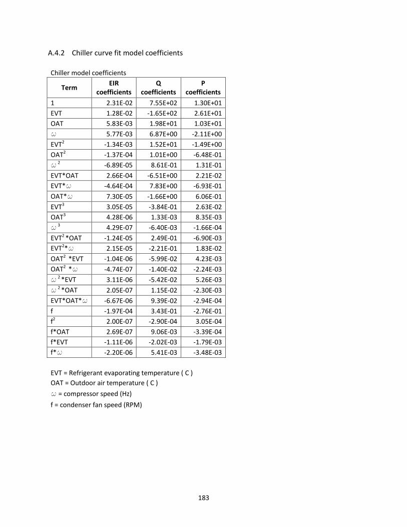
183
A.4.2 Chiller curve fit model coefficients
Chiller model coefficients
Term
EIR
coefficients
Q
coefficients
P
coefficients
1 2.31E-02 7.55E+02 1.30E+01
EVT 1.28E-02 -1.65E+02 2.61E+01
OAT 5.83E-03 1.98E+01 1.03E+01
w 5.77E-03 6.87E+00 -2.11E+00
EVT2 -1.34E-03 1.52E+01 -1.49E+00
OAT2 -1.37E-04 1.01E+00 -6.48E-01
w 2 -6.89E-05 8.61E-01 1.31E-01
EVT*OAT 2.66E-04 -6.51E+00 2.21E-02
EVT*w -4.64E-04 7.83E+00 -6.93E-01
OAT*w 7.30E-05 -1.66E+00 6.06E-01
EVT3 3.05E-05 -3.84E-01 2.63E-02
OAT3 4.28E-06 1.33E-03 8.35E-03
w 3 4.29E-07 -6.40E-03 -1.66E-04
EVT2 *OAT -1.24E-05 2.49E-01 -6.90E-03
EVT2*w 2.15E-05 -2.21E-01 1.83E-02
OAT2 *EVT -1.04E-06 -5.99E-02 4.23E-03
OAT2 *w -4.74E-07 -1.40E-02 -2.24E-03
w 2 *EVT 3.11E-06 -5.42E-02 5.26E-03
w 2 *OAT 2.05E-07 1.15E-02 -2.30E-03
EVT*OAT*w -6.67E-06 9.39E-02 -2.94E-04
f -1.97E-04 3.43E-01 -2.76E-01
f2 2.00E-07 -2.90E-04 3.05E-04
f*OAT 2.69E-07 9.06E-03 -3.39E-04
f*EVT -1.11E-06 -2.02E-03 -1.79E-03
f*w -2.20E-06 5.41E-03 -3.48E-03
EVT = Refrigerant evaporating temperature ( C )
OAT = Outdoor air temperature ( C )
w = compressor speed (Hz)
f = condenser fan speed (RPM)

184
A.4.3 Curve fit model linear regression code
The following Matlab codes identify the coefficients of curve-fit multivariable polynomial
models of the power consumption, cooling capacity, and the reciprocal of the coefficient of
performance (or electric input ratio EIR) of the split system air conditioner as a function of
outdoor air temperature, zone air temperature, compressor speed and condenser fan speed
and the chiller as a function of outdoor air temperature, evaporating temperature, compressor
speed and condenser fan speed.
function IdentifyACcurves()
%% function identifies the coefficients of the air conditioner's EIR model,
% cooling rate Q model, and power P model
% a 4-variable polynomial in compressor speed w, condenser fan speed f,
% outdoor air temperature x, and indoor zone air temperature z
format long
load CompMapData % load measured heat pump/chiller performanace data
% convert data structure objects to matlab matrices
for i=1:length(CompMapData)
z(i) = CompMapData(i).averages(14); % zone air temperature
x(i) = CompMapData(i).averages(17); % outdoor air temperature
w(i) = CompMapData(i).averages(56); % compressor speed
f(i) = CompMapData(i).averages(57); % condenser fan speed
p(i) = CompMapData(i).averages(33); % outdoor unit power consumption
q(i) = CompMapData(i).averages(50); % cooling load on the evaporator
end
z = z'; x = x'; q = q'; w = w'; f = f'; p = p'; % create column vectors
eir = p./q; % calculate late the EIR or 1/COP for each steady state conditions
% create the A matrix for the regressrion
A = [ones(size(z)) z x w (z.^2) (x.^2) (w.^2) (z.*x) (z.*w) (x.*w) ...
(z.^3) (x.^3) (w.^3) (z.^2).*x (z.^2).*w (x.^2).*z (x.^2).*w ...
(w.^2).*z (w.^2).*x z.*x.*w f f.^2 f.*z f.*x f.*w];
cEIR = regress(eir,A); % compute coefficients of the EIR curve
cQ = regress(q,A); % computer coefficients of the Q curve
cP = regress(p,A); % computer coefficients of the P curve
% save coefficients
save eircoefficients cEIR cQ cP
function IdentifyChillercurves()
%% function identifies the coefficients of the chiller's EIR model,
% cooling rate Q model, and power P model
% a 4-variable polynomial in compressor speed w, condenser fan speed f,
% outdoor air temperature x, and indoor zone air temperature z
format long
load CompMapData % load measured heat pump/chiller performanace data

185
% convert data structure objects to matlab matrices
for i=1:length(CompMapData)
e(i) = CompMapData(i).averages(16); % evaporating temperature
x(i) = CompMapData(i).averages(17); % outdoor air temperature
w(i) = CompMapData(i).averages(56); % compressor speed
f(i) = CompMapData(i).averages(57); % condenser fan speed
p(i) = CompMapData(i).averages(33); % outdoor unit power consumption
q(i) = CompMapData(i).averages(50); % cooling load on the evaporator
end
e = e'; x = x'; q = q'; w = w'; f = f'; p = p'; % create column vectors
eir = p./q; % calculate late the EIR or 1/COP for each steady state conditions
% create the A matrix for the regressrion
A = [ones(size(e)) e x w (e.^2) (x.^2) (w.^2) (e.*x) (e.*w) (x.*w) ...
(e.^3) (x.^3) (w.^3) (e.^2).*x (e.^2).*w (x.^2).*e (x.^2).*w ...
(w.^2).*e (w.^2).*x e.*x.*w f f.^2 f.*e f.*x f.*w];
cEIR = regress(eir,A); % compute coefficients of the EIR curve
cQ = regress(q,A); % computer coefficients of the Q curve
cP = regress(p,A); % computer coefficients of the P curve
% save coefficients
save eircoefficients cEIR cQ cP

186
Appendix B. Thermal model identification testing
B.1 Thermal test chamber components
B.1.1 Radiant concrete floor
The layout of the Warmboard radiant
subfloor, with grooves for pex pipe, is
shown at right. The groove spacing is 12
inches. Six parallel water loops were
installed, running down the length of the
floor and back from the system manifold.
The pressure drop per unit length of PEX is
0.016 psi/foot-pipe at 1 GPM for 1/2" PEX.
The total pressure drop in the system is less
than 1 foot of water column at the constant
flow rate of 2.1 GPM, with roughly 0.35
GPM per loop.
The PEX was installed in the Warmboard
grooves and three layers of concrete pavers
were installed over the top as shown in the
picture below right. The concrete pavers
have typical dimensions of eight inches by
16 inches by 1.5 inches, weighing 5.3
pounds. A picture of the radiant system
manifold is shown below left.

187
The Matlab code below is an approximate physical model of the concrete floor in the LLCS test
chamber. The greatest uncertainties in the model are the thermal conductivity of the concrete
pavers, the contact resistance between the Warmboard aluminum surface and the bottom of
the concrete pavers, and the contact resistance between the PEX pipe and the Warmboard
aluminum surface. The contact resistances between the pipe and aluminum and aluminum and
concrete pavers have been calibrated to match observations that show the typical temperature
difference between the chilled water and the bottom of the concrete pavers is around eight to
ten degrees Celsius. The thermal conductivity of the concrete pavers may vary anywhere
between 0.3 W/mK for very lightweight concrete to 1.5 W/mK for concrete. Over this range,
the percentage of the cooling delivered through the radiant floor lost to the outside of
chamber, through the bottom of the floor, varies anywhere from 15 to 30 percent. The 25
percent cooling energy loss apparent for the low lift predictive control of the TABS system in
Table 9 relative to the RCP system is within the range of possible losses from the floor.
function ModelConcreteFloor()
% Typical steady state temperature of the building slab and the chamber air
Tbuilding = 23+273; % temperature of building floor K
Tchamber = 23+273; % temperature of the chamber in K
Tchw = 7+273; % Typical chilled water temperature K
% Properties of the plywood subfloor
kplywood = 0.13; % thermal conductivity of plywood W/mK
Lplywood = 1.5*0.0254; % thickness of plywood in m
Aplywood = 12*17*0.3048*0.3048; % area of plywood per loop in m^2
UAplywood = (kplywood/Lplywood)*Aplywood; % conductance of plywood in W/K
Rplywood = 1/UAplywood; % resistance of plywood in K/W
% Properties of the floor joists
kjoist = 0.15; % thermal conductivity of wood stud W/mK
Ljoist = 3.5*0.0254; % thickness of joist m
Ajoist = (1.5/12)*17*12*0.3048*0.3048; % area of joist m2
UAjoist = (kjoist/Ljoist)*Ajoist; % conductance of joists in W/K
% Properties of the floor insulation
kinsulation = 0.03; % thermal conductivity of insulation W/mK
Linsulation = (3*0.0254); % thickness of insulation m
Ainsulation = (10.5/12)*17*12*0.3048*0.3048; % area of insulation m2
Rinsulation = Linsulation/kinsulation; % resistance of insulaion in m^2-K/W
Uinsulation = 1/Rinsulation; % U value of insulation in W/m^2-K
UAinsulation = Uinsulation*Ainsulation; % conductance of insulation in W/K
% Properties of the composite subfloor construction
UAjoistcomposite = UAjoist+UAinsulation % Total conductance of joist/insulation W/K
Rjoistcomposite = 1/UAjoistcomposite; % Total resistance of joist/insulation K/W
Rsubfloor = Rplywood+Rjoistcomposite; % Total resistance of subfloor in K/W
Rsubfloorperloop = 6*Rsubfloor; % Resistance of subfloor per loop of pipe in K/W
% Properties of the concrete paver/slab
m = 0.4535*15; % mass of one paver kg

188
volpaver = (1.75*8*16)*(0.0254^3) % volume of paver m3
rhopaver = m/volpaver; % concrete paver density kg/m^3
cp = 900; % concrete slab specific heat(J/kg-K)
Aconcrete =12*17*(0.3048^2); % concrete slab area m^2
kconcrete = 0.33; % lightweight concrete thermal conductivity W/m-K, ranging from 0.2-1.5 W/mK
Lconcrete = (1.75*3)*0.0254; % thickness of concrete m
Rslab = (Lconcrete/(kconcrete*Aconcrete)); % thermal resistance of slab K/W
Rfilm = 1/(10*Aconcrete); % radiative and convective resistance at slab surface K/W
Rslabfilmperloop = 6*(Rslab+Rfilm); % total resistance from bottom of slab to chamber in K/W
% properties of the chilled water
cp = 4200; % specific heat of water W/kg-K;
kwater = 0.6; % thermal conductivity of water in W/mK
rho = 1000; % density of water in kg/m3
mu = 0.0013; % dynamic viscosity of water in kg/m-s
nu = mu/rho; % kinematic viscosity of water in m2/s
% properties of the PEX chilled water pipe
GPM = 2.2 % Total chilled water flow rate in GPM
GPMperloop = GPM/6; % chilled water flow rate per loop
kPex = 0.45; % thermal conductivity of pex in W/mK
ID = 0.475 *0.0254; % inner diameter in m
OD = 0.625*0.0254; % outer diameter in m
Ac = pi*(ID/2)^2; % cross sectional area of pipes in m2
X = 12*0.0254/2; % half width of spacing between tubes in m
Um = GPMperloop*0.000063/Ac; % mean velocity of fluid in m/s
Pr = cp*mu/kwater; % Prandtl number of water
Re = Um*ID/nu; % Reynolds number of water
Lpipe = 17*2*0.3048; % length of pipe in m
% poperties of the aluminum subfloor surface
kAlum = 222; % thermal conducitivyt of aluminum in W/mK
tAlum = 0.03*0.0254/2; % half thickness of aluminum in m
% Calculate Nusselt number based on Reynolds number
if(Re>3000)
f = (0.790*log(Re)-1.64)^-2; % Friction factor
Nu = ((f/8)*(Re-1000)*Pr)/(1+(12.7*(f/8)^0.5*(Pr^(2/3)-1))); % Nusselt number for turbulent flow
disp(['Flow is turbulent, Nusselt number = ' num2str(Nu)])
elseif(Re>2300)
f = (0.790*log(Re)-1.64)^-2; % Friction factor
Nu = ((f/8)*(Re-1000)*Pr)/(1+(12.7*(f/8)^0.5*(Pr^(2/3)-1))); % Nusselt number for turbulent flow
Nu = mean([Nu 4]); % take mean of laminar and Gnielinski in transition region
disp(['Flow is transitional, Nusselt number = ' num2str(Nu)])
else
Nu = 4; % laminar region, not uniform temperature (3.66) or uniform heat flux (4.36)
disp(['Flow is laminar, Nusselt number = ' num2str(Nu)])
end
% Calculate heat transfer coefficient in the pipe using Nusselt number
h = Nu*kwater/ID; % W/m2K
%%

189
Rhc = 1/(pi*ID*h*Lpipe); % convective resistance K/W per loop
Rpipe = log(OD/ID)/(2*pi*kPex*Lpipe); % pipe wall resistance K/W per loop
Rcontactpipe = 0.003/(pi*OD*Lpipe); % pipe contact resistance K/W assume R = del-T/q/m2 = 0.3K/100 W/m2 =
0.003 m2-K/W
% aluminum to concrete contact resistance, calibrated to 10K difference
% between water and bottom of slab
Rcontactconcrete = (12*17*0.3048^2)*10/1200; % contact resistance m^2-K/W
Rcontactplywood = 0.05; % m2K/W assume R = del-T/q/m2 = 0.5K/100 W/m2 = 0.005 m2-K/W
% fin parameter (Perimeter Lpipe, Area = tAlum*Lpipe, h = 1/R_contact) for
% aluminum to concrete
mconcrete = (Lpipe/(kAlum*tAlum*Lpipe*Rcontactconcrete))^0.5;
RfintoSlab = ((Rcontactconcrete/(kAlum*tAlum*Lpipe*Lpipe))^0.5)*tanh(mconcrete*X)/2; % 1/2 resistance due to
two sides of aluminum on pipe
% fin parameter (Perimeter Lpipe, Area = tAlum*Lpipe, h = 1/R_contact) for
% aluminum to plywood
mplywood = (Lpipe/(kAlum*tAlum*Lpipe*Rcontactplywood))^0.5; % fin parameter (Perimeter L, Area = t*L, h =
1/R_contact)
RfintoPlywood = ((Rcontactplywood/(kAlum*tAlum*Lpipe*Lpipe))^0.5)*tanh(mplywood*X)/2; % 1/2 resistance
due to two sides of aluminum on pipe
Rwatertofinbase = (Rhc+Rpipe+Rcontactpipe); % resistance from water loop to base of fin K/W
Rchambertofinbase = RfintoSlab+Rslabfilmperloop; % resistance from chamber air to base of fin K/W
Rbuildingtofinbase = Rsubfloorperloop+RfintoPlywood; % resistance from building floor to base of fin K/W
% base of fin temperature, the aluminum temperature near the chilled water
% pipe
Tfinbase = (Tchw/Rwatertofinbase+Tchamber/(Rslab+Rfilm+RfintoSlab)+Tbuilding/(Rsubfloor+RfintoPlywood))/ ...
(1/Rwatertofinbase+1/(Rslab+Rfilm+RfintoSlab)+1/(Rsubfloor+RfintoPlywood));
% heat rate between the chamber and the aluminum near the chilled water
% pipe per loop
q1 = (Tchamber-Tfinbase)/Rchambertofinbase;
% heat rate between the building slab and the aluminum near the chilled
% water pipe per loop
q2 = (Tbuilding-Tfinbase)/Rbuildingtofinbase;
Q = (Tfinbase-Tchw)/Rwatertofinbase; % Total heat rate per loop
Qtot = Q*6 % Total heat rate from the floor
ChamberFraction = q1/(q1+q2)
BuildingFraction = q2/(q1+q2)
UST = Tfinbase+q1*RfintoSlab; % underslab temperature
PLT = Tfinbase+q2*RfintoPlywood; % plywood temperature
SST = Tchamber-q1*6*Rfilm; % Slab surface temperature
[Tchw-273 Tfinbase-273 PLT-273 UST-273 SST-273 Tbuilding-273 Tchamber-273]

190
An analysis of the diurnal heat capacity (DHC) of the concrete floor relative to its thickness, the
thermal conductivity of the concrete, and the heat transfer coefficient between the concrete
surface and the room air shows the relative importance of these different concrete slab and
heat transfer properties. DHC is a measure of the thermal storage capacity of a material,
measured by the total energy it can store and release in a diurnal cycle per degree of
temperature swing per unit area. The DHC of the slab as defined by Balcomb [1983b] is shown
in the graph below at left, for which the temperature swing of the concrete surface is used. In
general, increasing the depth of the concrete layer increases the DHC, or thermal storage
capacity, up to a certain depth after which storage capacity begins to decline. Depending on
the conductivity of the concrete, which may be as low as 0.2 W/mK for lightweight concrete,
the optimal concrete thicknes may range from five to fifteen centimeters. A concrete depth of
10 to 15 centimeters is optimal for typical values of concrete thermal conductivity.
The net heat transfer coefficient, in W/m2K, between the concrete surface and the chamber air
and other surfaces also affects the thermal storage capacity of the concrete slab. The graph
below at right shows the DHC relative to the zone air temperature swing for different values of
the net heat transfer coefficient between the concrete surface and the zone, including both
radiative and convective heat transfer. The DHC relative to the zone air temperature swing is
lower than the DHC defined by Balcomb [1983b] and is strongly affected by the value of the net
heat transfer coefficient. Slab depths greater than eight to twelve centimeters, for a typical
concrete thermconductivity, do not yield higher DHCs.
0 5 10 15 20 25 300
20
40
60
80
100
Depth (cm)
DHC Wh/m2K
Diurnal heat capacity relative to concrete surface temperature
(as defined by Balcomb [1983b]) as a function of concrete slab depth
for different concrete thermal conductivities in W/mK, h = 10 W/m2K
k = 0.2
k = 0.7
k = 1.2
k = 1.7
0 5 10 15 20 25 300
20
40
60
80
100
Depth (cm)
DHC Wh/m2K
Diurnal heat capacity relative to zone air temperature
as a function of concrete slab depth for different air to
concrete heat transfer coefficients in W/m2K, k = 1.2 W/mK
h = 5
h = 10
h = 15
h = 20
The Matlab code below calculates the DHC of a concrete slab as a function of depth, relative to
the concrete surface and relative to the zone air. function DHCslab(k,h)
% calculates the DHC of a concrete slab as a function of depth
% k is thermal conductivity in W/mK
% h is the net heat transfer coefficient between the slab surface and the
% zone in W/m^2 K

191
format long
depth = 0.01:0.01:0.3; % trial concrete depths in meters
admittance = zeros(length(depth),length(h));
segments = 12; % segmented concrete slab
TempSwing = 5; % diurnal air temperature swing
for i=1:length(depth)
rho = 2240; % concrete slabdensity kg/m^3
cp = 900; % concrete slab specific heat(J/kg-K)
area = 12*17*(0.3048^2); % concrete slab area m^2
Rfilm = 1/(h*area); % radiative and convective resistance at slab surface K/W
Cs = rho*cp*area*depth(i)/segments; % thermal capacity of slab J/K
Rconc = (depth(i)/(k*area))/(segments+1); % resistance of concrete K/W
inc = 60; % 1 minute increments
total = 60*60*24*4; % 4 days
ts = 0:inc:total'; % timesteps
u = 273+24+(TempSwing/2).*cos((2*pi/(24*60*60)).*ts); % room temperature driving function
% create state space model of concrete response, 12 segments
B = [1/((Rfilm+Rconc)*Cs) zeros(1,segments-1)]';
A = diag([ones(segments-1,1)*(-2/(Rconc*Cs)); -1/(Rconc*Cs)],0)+diag(ones(segments-
1,1)*(1/(Rconc*Cs)),1)+diag(ones(segments-1,1)*(1/(Rconc*Cs)),-1);
A(1,1) = -1/((Rfilm+Rconc)*Cs)-1/(Rconc*Cs);
% output air temperature and heat rate and surface temperature
C = [0 zeros(1,segments-1);...
-1/(Rfilm+Rconc) zeros(1,segments-1);...
Rfilm/(Rfilm+Rconc) zeros(1,segments-1)];
D = [1; 1/(Rfilm+Rconc); 1-Rfilm/(Rfilm+Rconc)];
x0 = (273+24).*ones(segments,1)';
sys = ss(A,B,C,D);
% simulate concrete floor state space model with sinusoidal room temperature driving function
[Y T X] = lsim(sys,u,ts,x0);
startindex = 60*24*2; endindex = 60*24*3;
delT = max(Y(startindex:endindex,1))-min(Y(startindex:endindex,1)); % air temperature swing
delQ = max(Y(startindex:endindex,2))-min(Y(startindex:endindex,2)); % thermal load swing
delST = max(Y(startindex:endindex,3))-min(Y(startindex:endindex,3)); % surface temperature swing
Q = sum(Y(find(Y(startindex:endindex,2)>0),2)/60); % total energy stored in a diurnal cycle
DHC(i) = Q/delST/area; % DHC per unit area
DHCair(i) = Q/delT/area; % DHC relative to air per unitarea
end
figure(1)
plot(depth*100,DHC)
hold all
plot(depth*100,DHCair)
xlabel('Depth (cm)')
ylabel('DHC Wh/m^2K')
title('Diurnal heat capacity as a function of concrete slab depth')

192
B.1.2 Internal Loads
The pictures on this page show the systems used to simulate
internal loads from people, equipment and lights. Clockwise
from the top right, the pictures show the simulated equipment
loads, the simulated load from occupants, the view of the inside
of a simulated internal load, and finally the lighting loads and the
ceiling mixing fan.
Inside the simulated equipment and occupant loads are three
light bulb sockets which can be used to change the amount of
load to achieve the different load densities described in chapter
6.
The ceiling fan was used to create some air movement to make
up for the concrete-core system cooling only from the floor, not
from the floor and ceiling. Also, the companion DOAS would
provide some air movement. The ceiling fan energy consumption
was counted as part of the internal loads, but not as part of the
system energy consumption. For an LLCS that required
supplemental air movement, much higher efficiency fans could
be used than that installed in the test chamber, which was
intended only to simulate the effects of cooling from above and
the DOAS.
During the temperature-CRTF model testing, the radiant heating
panels shown in the picture at bottom left were used to apply
internal radiant heating loads to the test chamber. A similar
system was installed underneath the concrete floor to apply
radiant thermal loads below the concrete floor prior to
installation of the chilled water piping. Electrical convective
heaters were used to simulate internal convective heating loads.

193
B.1.3 Climate chamber control
An image of the climate chamber HVAC control system is shown below. The system is a
constant air volume system comprising a supply, a return fan, a chilled water coil, an electric
pre-heat, an electric re-heat coil, and an economizer. The outdoor air supply and exhaust
dampers were fixed shut, the pre-heat coil was disabled, and the mixed air damper was fixed
open to force the system to only re-circulate indoor air. This was done to prevent humid
outside air from entering the climate chamber, and ultimately the test chamber, resulting in
latent loads. The system was programmed through time-of-day scheduling to follow the typical
summer week in climates of choice, including Atlanta and Phoenix.
The system is controlled by a Landis & Gyr System Powers 600 control system, with Insight
control software. This system is a predecessor to the Siemens Apogee control system.

194
B.2 Thermal test chamber sensors and instrumentation
B.2.1 Table of sensors for thermal test chamber Measurement description Sensor Make/Model Installation notes Accuracy
Air temperature measurements Omega/PR-T-24-SLE Installed at locations described in sections
B.2.2. Calibrated to measure within 0.01 K
0.5 C
(rated)
Surface temperature
measurements
Omega/PR-T-24-SLE Installed at locations described in sections
B.2.2. Calibrated to measure within 0.01 K
0.5 C
(rated)
Concrete slab and under-slab
temperature measurements
Omega/GG-T-28-SLE Installed at locations described in sections
B.2.2
0.5 C
(rated)
Convective heater power,
thermal model testing
F.W. Bell/PX-2221B1 Installed on the convective heat power supply 0.5 %
(rated)
Radiant ceiling panel power,
thermal model testing
F.W. Bell/PX-2221B1 Installed on the power supply to a variac,
which supplied the radaint ceiling panels.
0.5 %
(rated)
Radiant floor power, thermal
model testing
Voltage divider
DC current shunt
Internal load power Wattnode/
WNB-3Y-208P
Installed before a programmable switch relay. 0.5% of
reading
Radiant concrete-core floor
cooling rate
See Appendix C.2
The data for the thermal test chamber was logged by a Campbell Scientific CR10X data logger.
Three Campbell Scientific AM25T 25-channel multiplexers were used for logging thermocouple
temperature measurements. The reference temperature sensors of the three loggers were
calibrated relative to each other by enclosing the loggers in a well-insulated box and comparing
the steady state temperature measured by each logger’s reference temperature sensors. A
0.11 Kelvin offset for one of the loggers relative to the other two was identified and used to
correct the data from that logger. Accounting for this offset, the relative accuracy of the three
AM25T loggers is within 0.015 Kelvin. The internal loads were controlled using a Campbell
Scientific SDM-CD16AC 16 channel AC/DC controller. The CR10X data logging code is shown
below.
Thermal test chamber CR10X EdLog32 data-logging code (written primarily by P.R. Armstrong) ;{CR10X}
*Table 1 Program 01: 60 Execution Interval (seconds)
; First AM25T, control port 1 and 2 1: Do (P86) 1: 42 Set Port 2 High
2: Full Bridge (P6) 1: 1 Reps
2: 21 ñ 2.5 mV 60 Hz Rejection Range 3: 1 DIFF Channel 4: 1 Excite all reps w/Exchan 1
5: 250 mV Excitation 6: 1 Loc [ K_Vs_250 ] 7: 1.0 Mult
8: 0.0 Offset 3: Do (P86)
1: 41 Set Port 1 High
4: Do (P86) 1: 51 Set Port 1 Low 5: Full Bridge (P6)
1: 1 Reps 2: 4 ñ 500 mV Slow Range 3: 1 DIFF Channel
4: 1 Excite all reps w/Exchan 1 5: 250 mV Excitation
6: 2 Loc [ Vx_250 ] 7: .001 Mult 8: 0.0 Offset
6: Z=X/Y (P38) 1: 1 X Loc [ K_Vs_250 ] 2: 2 Y Loc [ Vx_250 ]
3: 4 Z Loc [ RefTemp_C ] 7: Z=X*F (P37)

195
1: 4 X Loc [ RefTemp_C ] 2: -.001 F
3: 4 Z Loc [ RefTemp_C ] 8: Z=X+F (P34)
1: 4 X Loc [ RefTemp_C ] 2: .09707 F 3: 4 Z Loc [ RefTemp_C ]
9: BR Transform Rf[X/(1-X)] (P59) 1: 1 Reps 2: 4 Loc [ RefTemp_C ]
3: 10.025 Mult (Rf) 10: Temperature RTD (P16)
1: 1 Reps 2: 4 R/R0 Loc [ RefTemp_C ] 3: 80 Loc [ RefTemp1C ]
4: 1.0 Mult 5: 0.0 Offset 11: Do (P86)
1: 52 Set Port 2 Low 12: Do (P86)
1: 42 Set Port 2 High 13: Beginning of Loop (P87) 1: 0 Delay
2: 25 Loop Count 14: Do (P86)
1: 41 Set Port 1 High 15: Do (P86) 1: 51 Set Port 1 Low
16: Do (P86) 1: 41 Set Port 1 High 17: Do (P86)
1: 51 Set Port 1 Low 18: Thermocouple Temp (DIFF) (P14)
1: 1 Reps 2: 21 ñ 2.5 mV 60 Hz Rejection Range 3: 1 DIFF Channel
4: 1 Type T (Copper-Constantan) 5: 80 Ref Temp Loc [ RefTemp1C ] 6: 5 -- Loc [ TC_1_1 ]
7: 1.0 Mult 8: 0.0 Offset
19: End (P95) 20: Do (P86) 1: 52 Set Port 2 Low
;Ssecond AM25T, control port 3 and 4 21: Do (P86)
1: 44 Set Port 4 High 22: Full Bridge (P6)
1: 1 Reps 2: 1 ñ 5 mV Slow Range 3: 1 DIFF Channel
4: 1 Excite all reps w/Exchan 1 5: 250 mV Excitation
6: 1 Loc [ K_Vs_250 ] 7: 1.0 Mult 8: 0.0 Offset
23: Do (P86) 1: 43 Set Port 3 High 24: Do (P86)
1: 53 Set Port 3 Low 25: Full Bridge (P6)
1: 1 Reps 2: 4 ñ 500 mV Slow Range 3: 1 DIFF Channel
4: 1 Excite all reps w/Exchan 1
5: 250 mV Excitation 6: 2 Loc [ Vx_250 ]
7: .001 Mult 8: 0.0 Offset
26: Z=X/Y (P38) 1: 1 X Loc [ K_Vs_250 ] 2: 2 Y Loc [ Vx_250 ]
3: 4 Z Loc [ RefTemp_C ] 27: Z=X*F (P37) 1: 4 X Loc [ RefTemp_C ]
2: -.001 F 3: 4 Z Loc [ RefTemp_C ]
28: Z=X+F (P34) 1: 4 X Loc [ RefTemp_C ] 2: .09707 F
3: 4 Z Loc [ RefTemp_C ] 29: BR Transform Rf[X/(1-X)] (P59) 1: 1 Reps
2: 4 Loc [ RefTemp_C ] 3: 10.025 Mult (Rf)
30: Temperature RTD (P16) 1: 1 Reps 2: 4 R/R0 Loc [ RefTemp_C ]
3: 81 Loc [ RefTemp2C ] 4: 1.0 Mult
5: 0.0 Offset 31: Do (P86) 1: 54 Set Port 4 Low
32: Do (P86) 1: 44 Set Port 4 High 33: Beginning of Loop (P87)
1: 0 Delay 2: 25 Loop Count
34: Do (P86) 1: 43 Set Port 3 High 35: Do (P86)
1: 53 Set Port 3 Low 36: Do (P86) 1: 43 Set Port 3 High
37: Do (P86) 1: 53 Set Port 3 Low
38: Thermocouple Temp (DIFF) (P14) 1: 1 Reps 2: 21 ñ 2.5 mV 60 Hz Rejection Range
3: 1 DIFF Channel 4: 1 Type T (Copper-Constantan) 5: 81 Ref Temp Loc [ RefTemp2C ]
6: 30 -- Loc [ TC_2_1 ] 7: 1.0 Mult
8: 0.0 Offset 39: End (P95) 40: Do (P86)
1: 54 Set Port 4 Low ;
;Third AM25T, control port 5 and 6 41: Do (P86) 1: 46 Set Port 6 High
42: Full Bridge (P6) 1: 1 Reps 2: 21 ñ 2.5 mV 60 Hz Rejection Range
3: 1 DIFF Channel 4: 1 Excite all reps w/Exchan 1
5: 250 mV Excitation 6: 1 Loc [ K_Vs_250 ] 7: 1.0 Mult
8: 0.0 Offset

196
43: Do (P86) 1: 45 Set Port 5 High
44: Do (P86) 1: 55 Set Port 5 Low
45: Full Bridge (P6) 1: 1 Reps 2: 4 ñ 500 mV Slow Range
3: 1 DIFF Channel 4: 1 Excite all reps w/Exchan 1 5: 250 mV Excitation
6: 2 Loc [ Vx_250 ] 7: .001 Mult
8: 0.0 Offset 46: Z=X/Y (P38) 1: 1 X Loc [ K_Vs_250 ]
2: 2 Y Loc [ Vx_250 ] 3: 4 Z Loc [ RefTemp_C ] 47: Z=X*F (P37)
1: 4 X Loc [ RefTemp_C ] 2: -.001 F
3: 4 Z Loc [ RefTemp_C ] 48: Z=X+F (P34) 1: 4 X Loc [ RefTemp_C ]
2: .09707 F 3: 4 Z Loc [ RefTemp_C ]
49: BR Transform Rf[X/(1-X)] (P59) 1: 1 Reps 2: 4 Loc [ RefTemp_C ]
3: 10.025 Mult (Rf) 50: Temperature RTD (P16) 1: 1 Reps
2: 4 R/R0 Loc [ RefTemp_C ] 3: 82 Loc [ RefTemp3C ]
4: 1.0 Mult 5: 0.0 Offset 51: Do (P86)
1: 56 Set Port 6 Low 52: Do (P86) 1: 46 Set Port 6 High
53: Beginning of Loop (P87) 1: 0 Delay
2: 25 Loop Count 54: Do (P86) 1: 45 Set Port 5 High
55: Do (P86) 1: 55 Set Port 5 Low 56: Do (P86)
1: 45 Set Port 5 High 57: Do (P86)
1: 55 Set Port 5 Low 58: Thermocouple Temp (DIFF) (P14) 1: 1 Reps
2: 21 ñ 2.5 mV 60 Hz Rejection Range 3: 1 DIFF Channel
4: 1 Type T (Copper-Constantan) 5: 82 Ref Temp Loc [ RefTemp3C ] 6: 55 -- Loc [ TC_3_1 ]
7: 1.0 Mult 8: 0.0 Offset 59: End (P95)
60: Do (P86) 1: 56 Set Port 6 Low ;
; CR10X measurements
;Chilled water pump power 61: Pulse (P3)
1: 1 Reps 2: 1 Pulse Channel 1 3: 20 High Frequency, Output Hz
4: 112 Loc [ PumpPower ] 5: 78.03 Multiplier 6: 0.0 Offset
; 0.867 CT AMPs, 338.2 ohms. 0.025 Wh/pulse/AMP
;Internal load power 62: Pulse (P3) 1: 1 Reps
2: 2 Pulse Channel 2 3: 20 High Frequency, Output Hz 4: 113 Loc [ LoadPower ]
5: 6 Multiplier 6: 0.0 Offset
; Load Watts, 0.6 W/Hz-CT-rated amps, 6 W/Hz, 0.0001667 Wh/pulse/Amp
;WRITE TO FINAL STORAGE 63: If time is (P92)
1: 0 Minutes into a 2: 1 Minute Interval 3: 10 Set Output Flag High
;assign array ID to final storage ID 64: Set Active Storage Area (P80)^20345 1: 1 Final Storage
2: 105 Array ID ;time stamp
65: Real Time (P77)^11008 1: 1210 Year,Day,Hour/Minute (prev day at midnight) ;input locations written to final storage
66: Resolution (P78) 1: 01 High Resolution 67: Sample (P70)^26349
1: 3 Reps 2: 80 Loc [ RefTemp1C ]
68: Sample (P70)^24951 1: 25 Reps 2: 5 Loc [ TC_1_1 ]
69: Sample (P70)^16309 1: 25 Reps 2: 30 Loc [ TC_2_1 ]
70: Sample (P70)^8277 1: 25 Reps
2: 55 Loc [ TC_3_1 ] 71: Average (P71)^15080 1: 1 Reps
2: 112 Loc [ PumpPower ] 72: Average (P71)^24514
1: 1 Reps 2: 113 Loc [ LoadPower ]
*Table 2 Program 02: 0.0 Execution Interval (seconds) *Table 3 Subroutines
End Program
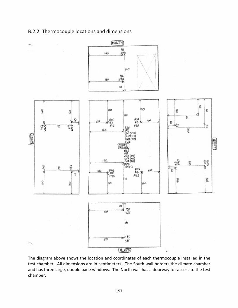
197
B.2.2 Thermocouple locations and dimensions
The diagram above shows the location and coordinates of each thermocouple installed in the
test chamber. All dimensions are in centimeters. The South wall borders the climate chamber
and has three large, double pane windows. The North wall has a doorway for access to the test
chamber.

198
B.3 Temperature-CRTF model identification codes
The code below identifies temperature-CRTF model coefficients from data logged by the Test Chamber CR10X and
the LLCS CR1000 data loggers. Thus, training data files come in pairs, one for the chamber and one for the LLCS
system, described in Appendix C. An arbitrary number of training data sets can be added to the list of training data
file names listed under the variables fnameschamber and fnameschiller, so long as they are in pairs and the data
has been corrected to account for records skipped by each logger.
function [ZATrmse MRTrmse OPTrmse USTrmse RWTrmse] = IdentifyTCRTF(minutes,order)
% function Identify TCRTF uses a set of training data files to identify the
% coefficients of a temperature-CRTF model for the zone air temperature
% ZAT, the mean radiant temperature MRT, the operative temperature OPT, the
% under-slab temperature UST, and the return water temperature RWT. The
% temperature CRTF applies a sampling interval of "minutes" and creates a
% model of order "order". The function returns the RMSE for each
% temperature-CRTF and saves the model coefficients
format long
%% Column labels for the test chamber data files
srcHdr={'id','yyyy','jd','hhmm','Tref1','Tref2','Tref3','xE1','xE2','xE3','xE4','xS1','xS2','xW1','xW2','xW3','xW4',... % 17
'xN1','xN2','xR1S','xR3S','xR1','xR3','xF1','xF2','xF3','xF4','xF5','x','x','x','x',... % 32
'E1','E2','E3','E4','S1','S2','R4','R5','R6','F3','F5','F6','CS1','CS2','CS3','S1S','S2S',... % 49
'E2S','E4S','R4S','R5S','R6S','F3S','F5S','F6S','W1','W2','W3','W4','N1','N2','R1','R2','R3',... % 66
'F1','F2','F4','CN1','CN2','CN3','N1S','N2S','W2S','W4S','R1S','R2S','R3S','F1S','F2S','F4S',... % 82
'PumpPower’,’LoadPower’}; % 86
%% Column labels for the chiller data files
chsrcHdr={'TIMESTAMP','RECORD','Tclimate_Avg','Tzone_Avg','Tcndair_Avg','dTcndair_Avg','Trhxliq_Avg', ...
'Trhxsh_Avg','Tchwreturn_Avg','Tchwsupply_Avg','Trsuc2_Avg','Trdis2_Avg','Trexvin2_Avg','Trexvout2_Avg', ...
'Wsystem_Avg','RunGPM_Avg','dutycycle_Avg','massflow_Avg'};
%% file names for all the training data sets. Two files are required for
% each training data set, one for the data logged from the test chamber
% CR10X and one for the data logged from the LLCS chiller CR1000
fnameschamber = {'FAN HI
OneMinuteChamberData.dat','AtlantaRadiantChamberData.dat','PhoenixRadiantChamberData.dat'};
fnameschiller = {'FAN HI
OneMinuteChillerData.dat','AtlantaRadiantChillerData.dat','PhoenixRadiantChillerData.dat'};
%% Initialize regression data matrices
AZAT = [];
bZAT = [];
AMRT = [];
bMRT = [];
AUST = [];
bUST = [];
ARWT = [];
bRWT = [];
AOPT = [];
bOPT = [];

199
%% loop through all of the training data sets
for k=1:length(fnameschamber)
fnamechamber = char(fnameschamber(k));
fnamechiller = char(fnameschiller(k));
% load the data-logger csv files
[QC Psys RWT OAT2 ZAT2] = LoadOneMinuteChillerDataIM(fnamechiller);
[QI AAT ZAT OAT OPT UST MRT Ppump chamtimes FLT] = LoadOneMinuteChamberDataIM(fnamechamber);
% sampling the data at interval "minutes" with five-minute averaging
nowmin = 1;
index = 1;
Ptot = Ppump+Psys; % Sum the chiller power and the chilled water pump power
while(nowmin+minutes<length(OPT)) % Loads in Watts QC30(index) = mean(QC(nowmin:nowmin+minutes-1)); QI30(index) = mean(QI(nowmin:nowmin+minutes-1)); % Temperatures in Kelvins RWT30(index) = mean(RWT(nowmin:nowmin+minutes-1))+273; AAT30(index) = mean(AAT(nowmin:nowmin+4))+273; ZAT30(index) = mean(ZAT(nowmin:nowmin+4))+273; ZAT230(index) = mean(ZAT2(nowmin:nowmin+4))+273; OAT30(index) = mean(OAT(nowmin:nowmin+4))+273; OAT230(index) = mean(OAT2(nowmin:nowmin+4))+273; OPT30(index) = mean(OPT(nowmin:nowmin+4))+273; UST30(index) = mean(UST(nowmin:nowmin+4))+273; FLT30(index) = mean(FLT(nowmin:nowmin+4))+273; MRT30(index) = mean(MRT(nowmin:nowmin+4))+273; % Energy in Watt-hours Ptot30(index) = mean(Ptot(nowmin:nowmin+minutes-1))*(60/minutes); % Power in Watts Ppump30(index) = mean(Ppump(nowmin:nowmin+minutes-1)); nowmin = nowmin+minutes; index = index+1; end
%% create regression data matrices from all of the training data sets
startindex = 1;
endindex = startindex+order;
while(endindex<=length(ZAT30))
AZAT = [AZAT; [ZAT30(startindex:endindex-1) AAT30(startindex:endindex) OAT30(startindex:endindex)
QC30(startindex:endindex) QI30(startindex:endindex)]];
bZAT = [bZAT; ZAT30(endindex)];
AMRT = [AMRT; [MRT30(startindex:endindex-1) AAT30(startindex:endindex) OAT30(startindex:endindex)
QC30(startindex:endindex) QI30(startindex:endindex)]];
bMRT = [bMRT; MRT30(endindex)];
AOPT = [AOPT; [OPT30(startindex:endindex-1) AAT30(startindex:endindex) OAT30(startindex:endindex)
QC30(startindex:endindex) QI30(startindex:endindex)]];
bOPT = [bOPT; OPT30(endindex)];
AUST = [AUST; [UST30(startindex:endindex-1) AAT30(startindex:endindex) OAT30(startindex:endindex)
QC30(startindex:endindex) QI30(startindex:endindex)]];
bUST = [bUST; UST30(endindex)];
if(Ppump30(endindex)>1) % Identify a 2nd order model for RWT ONLY when the pump is on
ARWT = [ARWT; [RWT30(endindex-2:endindex-1) UST30(endindex-2:endindex) QC30(endindex-
2:endindex)]];

200
bRWT = [bRWT; RWT30(endindex)];
end
startindex = startindex+1; endindex = endindex+1;
end
% steady-state heat transfer constraints on temperature-CRTFs
AeqOPT = [ones(1,order) ones(1,order+1) ones(1,order+1) zeros(1,order+1) zeros(1,order+1)];
beqOPT = 1;
AeqRWT = [ones(1,2) ones(1,3) zeros(1,3)];
beqRWT = 1;
% computer temperature-CRTF model coefficients
cZAT = lsqlin(AZAT,bZAT,[],[],AeqOPT,beqOPT);
cMRT = lsqlin(AMRT,bMRT,[],[],AeqOPT,beqOPT);
cOPT = lsqlin(AOPT,bOPT,[],[],AeqOPT,beqOPT);
cUST = lsqlin(AUST,bUST,[],[],AeqOPT,beqOPT);
cRWT = lsqlin(ARWT,bRWT,[],[],AeqRWT,beqRWT);
% computer temperature-CRTF RMSEs
ZATrmse = mean((bZAT-AZAT*cZAT).^2).^0.5;
MRTrmse = mean((bMRT-AMRT*cMRT).^2).^0.5;
OPTrmse = mean((bOPT-AOPT*cOPT).^2).^0.5;
USTrmse = mean((bUST-AUST*cUST).^2).^0.5;
RWTrmse = mean((bRWT-ARWT*cRWT).^2).^0.5;
end
save thermalmodels cZAT cMRT cUST cRWT cOPT
The code below validates temperature-CRTF models from data logged by the Test Chamber CR10X and the LLCS
CR1000 data loggers. Like the training data, validation data files come in pairs, one for the chamber and one for
the LLCS system, described in Appendix C. An arbitrary number of validation data sets can be added to the list of
validation data file names listed under the variables fnameschamber and fnameschiller, so long as they are in pairs
and the data has been fixed to account for skipped records by each logger. The validate code will compute the
root mean square error, in Kelvin, for predictions of zone air temperature (ZAT), mean radiant temperature (MRT),
operative temperature (OPT), under-slab temperature (UST), and return water temperature (RWT) up to the
number of look-ahead-hours selected by the input “lookaheadhours”.
function [ZATrmse MRTrmse OPTrmse USTrmse RWTonrmse] = ValidateTCRTF(minutes,order,lookaheadhours)
%% function ValidateTCRTF computes the RMSE of the temperature-CRTF models
% applied to one validation data set (not used in training) for
% temperature-CRTF models with sampling intervals of "minutes" minutes and
% of order "order". The RMSE is computed for the a look-ahead predictive
% horizon that is "lookaheadhours" hours ahead. The RMSE of the models
% relative to the validation data is computed and stored
format long
% load the temperature-CRTF model coefficients
load thermalmodels
%% Column labels for the test chamber data files
srcHdr={'id','yyyy','jd','hhmm','Tref1','Tref2','Tref3','xE1','xE2','xE3','xE4','xS1','xS2','xW1','xW2','xW3','xW4',... % 17

201
'xN1','xN2','xR1S','xR3S','xR1','xR3','xF1','xF2','xF3','xF4','xF5','x','x','x','x',... % 32
'E1','E2','E3','E4','S1','S2','R4','R5','R6','F3','F5','F6','CS1','CS2','CS3','S1S','S2S',... % 49
'E2S','E4S','R4S','R5S','R6S','F3S','F5S','F6S','W1','W2','W3','W4','N1','N2','R1','R2','R3',... % 66
'F1','F2','F4','CN1','CN2','CN3','N1S','N2S','W2S','W4S','R1S','R2S','R3S','F1S','F2S','F4S',... % 82
'RCPwr','RFPrBad','RFamps','RFPwr'}; % 86
%% Column labels for the chiller data files
chsrcHdr={'TIMESTAMP','RECORD','Tclimate_Avg','Tzone_Avg','Tcndair_Avg','dTcndair_Avg','Trhxliq_Avg', ...
'Trhxsh_Avg','Tchwreturn_Avg','Tchwsupply_Avg','Trsuc2_Avg','Trdis2_Avg','Trexvin2_Avg','Trexvout2_Avg', ...
'Wsystem_Avg','RunGPM_Avg','dutycycle_Avg','massflow_Avg'};
%% file names for all the validation data sets. Two files are required for
% each validation data set, one for the data logged from the test chamber
% CR10X (chamber) and one for the data logged from the LLCS (chiller) CR1000
fnames = {'VAL2 HI OneMinuteChamberData.dat'};
fnameschiller = {'VAL2 HI OneMinuteChillerData.dat'};
%% loop through chamberdata sets
fnamechamber = char(fnames(1));
fnamechiller = char(fnameschiller(1));
% load the data-logger csv files
[QC Psys RWT OAT2 ZAT2 chilltimes] = LoadOneMinuteChillerDataIM(fnamechiller);
[QI AAT ZAT OAT OPT UST MRT Ppump chamtimes FLT] = LoadOneMinuteChamberDataIM(fnamechamber);
% sampling the data at interval "minutes" with five-minute averaging
nowmin = 1;
index = 1;
Ptot = Ppump+Psys;
while(nowmin+minutes<length(OPT))
% Loads in Watts
QC30(index) = mean(QC(nowmin:nowmin+minutes-1));
QI30(index) = mean(QI(nowmin:nowmin+minutes-1));
% Temperatures in Kelvin
RWT30(index) = mean(RWT(nowmin:nowmin+minutes-1))+273;
AAT30(index) = mean(AAT(nowmin:nowmin+4))+273;
ZAT30(index) = mean(ZAT(nowmin:nowmin+4))+273;
ZAT230(index) = mean(ZAT2(nowmin:nowmin+4))+273;
OAT30(index) = mean(OAT(nowmin:nowmin+4))+273;
OAT230(index) = mean(OAT2(nowmin:nowmin+4))+273;
OPT30(index) = mean(OPT(nowmin:nowmin+4))+273;
UST30(index) = mean(UST(nowmin:nowmin+4))+273;
MRT30(index) = mean(MRT(nowmin:nowmin+4))+273;
%Energy in Watt-hours
Ptot30(index) = mean(Ptot(nowmin:nowmin+minutes-1))*(60/minutes);
% Power in Watts
Ppump30(index) = mean(Ppump(nowmin:nowmin+minutes-1));
nowmin = nowmin+minutes;
index = index+1;
end
% move through the entire validation data, for each data set, from the

202
% beginning of the data to the end, less the number of
% look-ahead-hours, to predict temperatures "lookaheadhours" hours ahead
% beginning with a segment of data order+1 samples long. Starting with
% data samples 1 to order+1, predicting out to order+1+lookaheadsteps,
% then with samples 2 order+2, predicting out to
% order+1+lookaheadsteps, etc...
startpoint=1;
endpoint = startpoint+order;
% number of samples ahead to predict for a given sampling interval to
% predict "lookaheadhours" hours ahead
lookaheadsteps = lookaheadhours*(60/minutes);
while(endpoint+lookaheadsteps<length(ZAT30))
endpoint = startpoint+order;
% initialize matrices f
AOPT = [];
AZAT = [];
AMRT = [];
AUST = [];
ARWT = [];
RWTpredon=[];
RWT30ton=[];
% initialize the data from which the "lookaheadhour"-hour-ahead
% prediction will be made
RWTpred = RWT30(startpoint:endpoint-1);
MRTpred = MRT30(startpoint:endpoint-1);
OPTpred = OPT30(startpoint:endpoint-1);
USTpred = UST30(startpoint:endpoint-1);
ZATpred = ZAT30(startpoint:endpoint-1);
QC30t = QC30(startpoint:startpoint+order+lookaheadsteps);
QI30t = QI30(startpoint:startpoint+order+lookaheadsteps);
RWT30t = RWT30(startpoint:startpoint+order+lookaheadsteps);
AAT30t = AAT30(startpoint:startpoint+order+lookaheadsteps);
ZAT30t = ZAT30(startpoint:startpoint+order+lookaheadsteps);
OAT30t = OAT30(startpoint:startpoint+order+lookaheadsteps);
OPT30t = OPT30(startpoint:startpoint+order+lookaheadsteps);
UST30t = UST30(startpoint:startpoint+order+lookaheadsteps);
MRT30t = MRT30(startpoint:startpoint+order+lookaheadsteps);
% for the segment of data being used for prediction, predict the
% temperatures ahead from step 1 to step lookaheadsteps (which is
% sampling interval and model order dependent)
startindex = 1;
endindex = startindex+order;
pumponindex=1; % track the time the pump is on independently
while(endindex<=1+order+lookaheadsteps) % loop until all "lookaheadsteps" predictions have been made
AZAT = [ZATpred(startindex:endindex-1) AAT30t(startindex:endindex) OAT30t(startindex:endindex)
QC30t(startindex:endindex) QI30t(startindex:endindex)];
ZATpred(endindex) = AZAT*cZAT;
AMRT = [MRTpred(startindex:endindex-1) AAT30t(startindex:endindex) OAT30t(startindex:endindex)
QC30t(startindex:endindex) QI30t(startindex:endindex)];
MRTpred(endindex) = AMRT*cMRT;

203
AOPT = [OPTpred(startindex:endindex-1) AAT30t(startindex:endindex) OAT30t(startindex:endindex)
QC30t(startindex:endindex) QI30t(startindex:endindex)];
OPTpred(endindex) = AOPT*cOPT;
AUST = [USTpred(startindex:endindex-1) AAT30t(startindex:endindex) OAT30t(startindex:endindex)
QC30t(startindex:endindex) QI30t(startindex:endindex)];
USTpred(endindex) = AUST*cUST;
if(Ppump30(endindex)>1) % if the pump is on
ARWT = [RWT30t(endindex-2:endindex-1) UST30t(endindex-2:endindex) QC30t(endindex-2:endindex)];
RWTpred(endindex) = ARWT*cRWT;
RWT30ton(pumponindex) = RWT30t(endindex); % compile the actual RWT data while the pump is on
RWTpredon(pumponindex) = RWTpred(endindex); % predict RWT from its transfer function model
pumponindex = pumponindex+1;
else
RWTpred(endindex) = OAT30t(endindex); % if the pump is off, assume RWT floats to ambient
temperature
end
startindex = startindex+1; endindex = endindex+1; % proceed to predict next time step
end
% compute the mean square error and relative mean square error for each
% model for the current set of predictions
ZATmse(startpoint) = mean((ZAT30t-ZATpred).^2);
ZATrelmse(startpoint) = mean(((ZAT30t-ZATpred)./(max(ZAT30t)-min(ZAT30t))).^2);
MRTmse(startpoint) = mean((MRT30t-MRTpred).^2);
MRTrelmse(startpoint) = mean(((MRT30t-MRTpred)./(max(MRT30t)-min(MRT30t))).^2);
OPTmse(startpoint) = mean((OPT30t-OPTpred).^2);
OPTrelmse(startpoint) = mean(((OPT30t-OPTpred)./(max(OPT30t)-min(OPT30t))).^2);
USTmse(startpoint) = mean((UST30t-USTpred).^2);
USTrelmse(startpoint) = mean(((UST30t-USTpred)./(max(UST30t)-min(UST30t))).^2);
if(~isempty(RWTpredon) && ~isempty(RWT30t) )
RWTonmse(startpoint) = mean((RWT30ton-RWTpredon).^2);
RWTonrelmse(startpoint) = mean(((RWT30ton-RWTpredon)./(max(RWT30ton)-min(RWT30ton))).^2);
end
startpoint= startpoint+1;
endpoint=endpoint+1;
end
% compute the RMSE and relative RMSE for the entire validation data set,
% for all predictions based on all possible segments of data
ZATrmse = mean(ZATmse).^0.5
ZATrelrmse = mean(ZATrelmse).^0.5
MRTrmse = mean(MRTmse).^0.5
MRTrelrmse = mean(MRTrelmse).^0.5
OPTrmse = mean(OPTmse).^0.5
OPTrelrmse = mean(OPTrelmse).^0.5
USTrmse = mean(USTmse).^0.5
USTrelrmse = mean(USTrelmse).^0.5
RWTonrmse = mean(RWTonmse).^0.5
RWTonrelrmse = mean(RWTonrelmse).^0.5
save ALLRMSES ZATrmse ZATrelrmse MRTrmse MRTrelrmse OPTrmse OPTrelrmse USTrmse USTrelrmse
RWTonrmse RWTonrelrmse
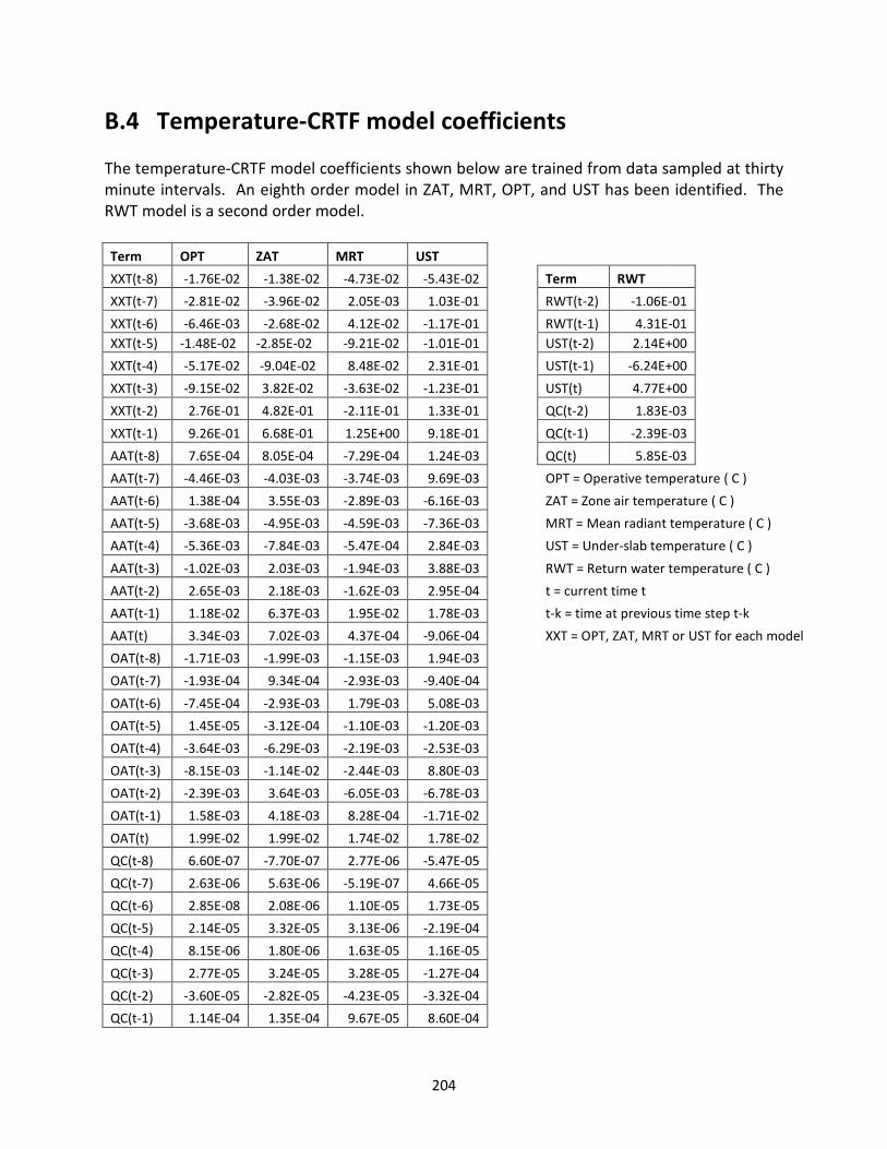
204
B.4 Temperature-CRTF model coefficients
The temperature-CRTF model coefficients shown below are trained from data sampled at thirty
minute intervals. An eighth order model in ZAT, MRT, OPT, and UST has been identified. The
RWT model is a second order model.
Term OPT ZAT MRT UST
XXT(t-8) -1.76E-02 -1.38E-02 -4.73E-02 -5.43E-02 Term RWT
XXT(t-7) -2.81E-02 -3.96E-02 2.05E-03 1.03E-01 RWT(t-2) -1.06E-01
XXT(t-6) -6.46E-03 -2.68E-02 4.12E-02 -1.17E-01 RWT(t-1) 4.31E-01
XXT(t-5) -1.48E-02 -2.85E-02 -9.21E-02 -1.01E-01 UST(t-2) 2.14E+00
XXT(t-4) -5.17E-02 -9.04E-02 8.48E-02 2.31E-01 UST(t-1) -6.24E+00
XXT(t-3) -9.15E-02 3.82E-02 -3.63E-02 -1.23E-01 UST(t) 4.77E+00
XXT(t-2) 2.76E-01 4.82E-01 -2.11E-01 1.33E-01 QC(t-2) 1.83E-03
XXT(t-1) 9.26E-01 6.68E-01 1.25E+00 9.18E-01 QC(t-1) -2.39E-03
AAT(t-8) 7.65E-04 8.05E-04 -7.29E-04 1.24E-03 QC(t) 5.85E-03
AAT(t-7) -4.46E-03 -4.03E-03 -3.74E-03 9.69E-03 OPT = Operative temperature ( C )
AAT(t-6) 1.38E-04 3.55E-03 -2.89E-03 -6.16E-03 ZAT = Zone air temperature ( C )
AAT(t-5) -3.68E-03 -4.95E-03 -4.59E-03 -7.36E-03 MRT = Mean radiant temperature ( C )
AAT(t-4) -5.36E-03 -7.84E-03 -5.47E-04 2.84E-03 UST = Under-slab temperature ( C )
AAT(t-3) -1.02E-03 2.03E-03 -1.94E-03 3.88E-03 RWT = Return water temperature ( C )
AAT(t-2) 2.65E-03 2.18E-03 -1.62E-03 2.95E-04 t = current time t
AAT(t-1) 1.18E-02 6.37E-03 1.95E-02 1.78E-03 t-k = time at previous time step t-k
AAT(t) 3.34E-03 7.02E-03 4.37E-04 -9.06E-04 XXT = OPT, ZAT, MRT or UST for each model
OAT(t-8) -1.71E-03 -1.99E-03 -1.15E-03 1.94E-03
OAT(t-7) -1.93E-04 9.34E-04 -2.93E-03 -9.40E-04
OAT(t-6) -7.45E-04 -2.93E-03 1.79E-03 5.08E-03
OAT(t-5) 1.45E-05 -3.12E-04 -1.10E-03 -1.20E-03
OAT(t-4) -3.64E-03 -6.29E-03 -2.19E-03 -2.53E-03
OAT(t-3) -8.15E-03 -1.14E-02 -2.44E-03 8.80E-03
OAT(t-2) -2.39E-03 3.64E-03 -6.05E-03 -6.78E-03
OAT(t-1) 1.58E-03 4.18E-03 8.28E-04 -1.71E-02
OAT(t) 1.99E-02 1.99E-02 1.74E-02 1.78E-02
QC(t-8) 6.60E-07 -7.70E-07 2.77E-06 -5.47E-05
QC(t-7) 2.63E-06 5.63E-06 -5.19E-07 4.66E-05
QC(t-6) 2.85E-08 2.08E-06 1.10E-05 1.73E-05
QC(t-5) 2.14E-05 3.32E-05 3.13E-06 -2.19E-04
QC(t-4) 8.15E-06 1.80E-06 1.63E-05 1.16E-05
QC(t-3) 2.77E-05 3.24E-05 3.28E-05 -1.27E-04
QC(t-2) -3.60E-05 -2.82E-05 -4.23E-05 -3.32E-04
QC(t-1) 1.14E-04 1.35E-04 9.67E-05 8.60E-04

205
Term OPT ZAT MRT UST
QC(t) -1.08E-06 1.03E-06 -2.66E-06 6.90E-05
QI(t-8) 7.90E-05 1.28E-04 1.05E-05 -1.62E-05
QI(t-7) -2.46E-06 1.58E-05 -1.66E-05 -2.62E-05
QI(t-6) -1.35E-04 -1.03E-04 -1.04E-04 -4.12E-05
QI(t-5) 7.77E-05 1.89E-04 -9.75E-06 1.41E-04
QI(t-4) -8.99E-05 -2.50E-04 -1.71E-04 9.44E-05
QI(t-3) -5.46E-04 -1.15E-03 -4.76E-05 -1.22E-04
QI(t-2) -9.88E-04 -1.19E-03 -6.21E-04 1.44E-04
QI(t-1) 1.47E-03 2.03E-03 1.08E-03 3.97E-04
QI(t) 2.72E-04 5.34E-04 -1.11E-06 -4.04E-04

206
Appendix C. LLCS system testing
C.1 LLCS and SSAC components
Component Description Make/Model
Chiller/AC
outdoor unit
This component contains the compressor, condenser
fan, condenser heat exchanger, inverters and
electronics supplying both the SSAC and the LLCS
Mitsubishi
MUZ-A09NA-1
AC indoor unit This is the air-heated evaporator used for the SSAC,
containing the finned-tube evaporator heat
exchanger and the evaporator fan
Mitsubishi
MSZ-A09NA
Brazed plate heat
exchanger
The BPHX is a counter-flow heat exchanger between
R410A and the chilled water
Flatplate
GB240-H10
Chilled water
pump
The chilled water pump is installed on the supply
side to the radiant floor
Laing
D5 strong w/PWM
P/N: P311
Radiant subfloor The radiant subfloor, made by Warmboard, is a 5/8”
plywood subfloor, topped by 0.03” aluminum, with
1/2" grooves at 12” spacing for PEX pipe installation
Warmboard
Chilled water
pipe and fittings
The chilled water piping is constructed of PEX pipe
embedded in the grooves of the Warmboard radiant
subfloor.
Uponor
1/2” hePex with
ProPex fittings
Radiant manifold 6-loop engineered plastic (EP) radiant manifold with
flow meters.
Uponor
PEXsupply
SKU: A2670601

207
C.2 LLCS sensors and instrumentation Table of sensors, make and model Label Sensor
description
Sensor Make/Model Installation notes Accuracy
Ts Suction
refrigerant
temperature
Omega/PR-T-24-SLE Insulated pipe surface measurement 0.5 C
(rated)
Td Discharge
refrigerant
temperature
Omega/PR-T-24-SLE Insulated pipe surface measurement 0.5 C
(rated)
Tcnd Refrigerant
condensing
temperature
Omega/PR-T-24-SLE Insulated pipe surface measurement 0.5 C
(rated)
Tcnd,liq Condenser
outlet liquid
refrigerant
temperature
Omega/PR-T-24-SLE Insulated pipe surface measurement 0.5 C
(rated)
Txvi Expansion valve
inlet refrigerant
temperature
Omega/PR-T-24-SLE Insulated pipe surface measurement 0.5 C
(rated)
Txvo Expansion valve
outlet
refrigerant
temperature
Omega/PR-T-24-SLE Insulated pipe surface measurement 0.5 C
(rated)
Thxi Brazed plate
heat exchanger
inlet refrigerant
temperature
Omega/PR-T-24-SLE Insulated pipe surface measurement 0.5 C
(rated)
Thxo Brazed plate
heat exchanger
outlet
refrigerant
temperature
Omega/PR-T-24-SLE Insulated pipe surface measurement 0.5 C
(rated)
Tcnd,air,in Condenser inlet
air temperature
Omega/PR-T-24-SLE Installed in condense rair inlet stream 0.5 C
(rated)
Tevp Refrigerant
evaporating
temperature
Omega/PR-T-24-SLE Insulated pipe surface measurement 0.5 C
(rated)
∆Tcnd,air Condenser air
temperature
difference
Omega/PR-T-24-SLE
16 junction thermopile
A 16 junction thermopile 0.5 C
(rated)
Ps Suction
refrigerant
pressure
MEAS, INC
MSP-300-500-P2-N1
Installed in the suction service port 1% of span
Pd Discharge
refrigerant
pressure
MEAS, INC
MSP-300-1000-P2-N1
Installed in the discharge service port 1% of span
Pxvi Expansion valve
inlet refrigerant
pressure
MEAS, INC
MSP-300-1000-P2-N1
Installed in the liquid line 1% of span

208
Pxvo Expansion valve
outlet
refrigerant
pressure
MEAS, INC
MSP-300-500-P2-N1
Installed after the stop valve downstream
of the expansion valve
1% of span
refm& Refrigerant mass
flowrate
Micromotion
Meter:
CMFS015M323N2BAEZZZ
Transmitter:
2500D3ABBAEZZZ
A Micromotion Coriolis mass flow meter
was installed in the liquid line, with
roughly 5 feet of head.
0.05% of
rate
Wunit Total power to
the outdoor
unit, including
inverters,
condenser fan
and compressor
Wattnode
WNB-3D-240-P
Installed on the 208VAC power supply to
the outdoor unit
0.5% of
reading
W3∅,cmp Three phase
power from the
inverter to the
compressor
Yokogawa
WT230
Installed between the compressor inverter
and the compressor
0.1% of
reading
RWT Chilled water
return
temperature
Omega
TMTSS-062G-6
Installed in the chilled water return pipe
immediately exiting the chamber
0.5 C
(rated)
SWT Chilled water
supply
temperature
Omega
TMTSS-062G-6
Installed in the chilled water supply pipe
just before entering the chamber
0.5 C
(rated)
" Chilled water
volumetric
flowrate
Omega
FTB8007B
Installed in the chilled water return line 1.5 % of
reading
WQI Total power to
the internal
loads
Wattnode
WNB-3Y-208-P
Installed on a power strip, to which all
internal loads were connected
0.5% of
reading
Wp Total power to
the chilled water
pump
Wattnode
WNB-3Y-208-P
Installed on the 120VAC power supplied
to the chilled water pump power supply
0.5% of
reading
The data measured from the LLCS test system was logged using a Campbell Scientific CR1000
data logger, with a slave Campbell Scientific AM25T 25-channel multiplexer for thermocouple
measurements. The control code for the CR1000 data logger is shown below, and includes the
control code for operating the internal loads and turning on the chilled water pump any time
the chiller is in operation.
'CR1000 LLCS data logging, load control, and pump switching
'Declare Variables and Units
Public BattV
Public Pxvout, Pxvin, Pdis, Psuc 'Pressure measurements
''Trsuc-1, Trdis-2, Trxvin-3, Trxvout-4, Tcndliq-5, Tcnd-6, Tcndmix-7, Trevp-8, Trhxsh-9, Trhxliq-10
'Public Ref_Temps(10)
Public Trsuc, Trdis, Trxvin, Trxvout, Trcndliq, Trcnd, Trcndmix, Trevp, Trhxsh, Trhxliq, Trsuc2, Trdis2, Trexvin2,
Trexvout2, Tsh
Public dTcndair 'channel 11

209
Public Tclimate, Tcndair, Tzone
Public Tchwreturn, Tchwsupply, Qcool
'Tclimate-12, Tcndair-13, Tzone-14
'Public Air_Temps(3)
Public RTemp_C
Public massflow, density
Public Wloads, Wsystem, Wpump, WsysAVG
Public FanSpd, CmpSpd
Public delta_mV, TdTref, dTresult, mV_TdT, i
Public Source(16)
Public DateArray(9)
Public dutycycle, Period, GPM, RunGPM, dutycycleprev
Public VaisT, RH, DT, a, b, gamma, DTplus2, ACYoko, BCYoko, Tot3ph
Units BattV=Volts
'Define Data Tables
DataTable(Table1,True,-1)
DataInterval (0,0,Sec,10)
Minimum (1,BattV,FP2,0,0)
Sample(1,Tclimate,FP2)
Sample(1,Tzone,FP2)
Sample(1,Tcndair,FP2)
Sample(1,dTcndair,FP2)
Sample(1,Trsuc,FP2)
Sample(1,Trdis,FP2)
Sample(1,Trxvin,FP2)
Sample(1,Trxvout,FP2)
Sample(1,Trcnd,FP2)
Sample(1,Trcndmix,FP2)
Sample(1,Trcndliq,FP2)
Sample(1,Trevp,FP2)
Sample(1,Trhxliq,FP2)
Sample(1,Trhxsh,FP2)
Sample(1,Tchwreturn,FP2)
Sample(1,Tchwsupply,FP2)
Sample(1,Trsuc2,FP2)
Sample(1,Trdis2,FP2)
Sample(1,Trexvin2,FP2)
Sample(1,Trexvout2,FP2)
Sample(1,Psuc,FP2)
Sample(1,Pdis,FP2)
Sample(1,Pxvin,FP2)
Sample(1,Pxvout,FP2)
Sample(1,Wloads,FP2)
Sample(1,Wsystem,FP2)
Sample(1,FanSpd,FP2)
Sample(1,CmpSpd,FP2)
Sample(1,GPM,FP2)
Sample(1,RunGPM,FP2)
Sample(1,dutycycle,FP2)
Sample(1,Tsh,FP2)
Sample(1,massflow,FP2)

210
Sample(1,density,FP2)
Sample(1,VaisT,FP2)
Sample(1,RH,FP2)
Sample(1,Qcool,FP2)
EndTable
DataTable(Table2,True,-1)
DataInterval (0,1,Min,10)
Average(1,Tclimate,FP2,False)
Average(1,Tzone,FP2,False)
Average(1,Tcndair,FP2,False)
Average(1,dTcndair,FP2,False)
Average(1,Trhxliq,FP2,False)
Average(1,Trhxsh,FP2,False)
Average(1,Tchwreturn,FP2,False)
Average(1,Tchwsupply,FP2,False)
Average(1,Trsuc2,FP2,False)
Average(1,Trdis2,FP2,False)
Average(1,Trexvin2,FP2,False)
Average(1,Trexvout2,FP2,False)
Average(1,Wsystem,FP2,False)
Average(1,RunGPM,FP2,False)
Average(1,dutycycle,FP2,False)
Average(1,massflow,FP2,False)
Average(1,RH,FP2,False)
Average(1,Qcool,FP2,False)
Average(1,ACYoko,FP2,False)
Average(1,BCYoko,FP2,False)
EndTable
'Main Program
BeginProg
Scan(1,Sec,1,0)
'Default Datalogger Battery Voltage measurement BattV
Battery(BattV)
'Reference Temperature measurement RTemp_C on the AM25T Multiplexer:
AM25T(RTemp_C,0,mV2_5C,1,1,TypeT,RTemp_C,7,8,Vx2,True,0,250,1,0)
'Temperature Measurements
AM25T (Trsuc,1,mV2_5C,1,8,TypeT,RTemp_C,7,8,Vx2,True ,0,250,1.0,0)
AM25T (Trdis,1,mV2_5C,2,8,TypeT,RTemp_C,7,8,Vx2,True ,0,250,1.0,0)
AM25T (Trxvin,1,mV2_5C,3,8,TypeT,RTemp_C,7,8,Vx2,True ,0,250,1.0,0)
AM25T (Trxvout,1,mV2_5C,4,8,TypeT,RTemp_C,7,8,Vx2,True ,0,250,1.0,0)
AM25T (Trcndliq,1,mV2_5C,5,8,TypeT,RTemp_C,7,8,Vx2,True ,0,250,1.0,0)
AM25T (Trcnd,1,mV2_5C,6,8,TypeT,RTemp_C,7,8,Vx2,True ,0,250,1.0,0)
AM25T (Trcndmix,1,mV2_5C,7,8,TypeT,RTemp_C,7,8,Vx2,True ,0,250,1.0,0)
AM25T (Trevp,1,mV2_5C,8,8,TypeT,RTemp_C,7,8,Vx2,True ,0,250,1.0,0)
AM25T (Trhxsh,1,mV2_5C,9,8,TypeT,RTemp_C,7,8,Vx2,True ,0,250,1.0,0)
AM25T (Trhxliq,1,mV2_5C,10,8,TypeT,RTemp_C,7,8,Vx2,True ,0,250,1.0,0)
AM25T (Tclimate,1,mV2_5C,12,8,TypeT,RTemp_C,7,8,Vx2,True ,0,250,1.0,0)
AM25T (Tcndair,1,mV2_5C,13,8,TypeT,RTemp_C,7,8,Vx2,True ,0,250,1.0,0)
AM25T (Tzone,1,mV2_5C,14,8,TypeT,RTemp_C,7,8,Vx2,True ,0,250,1.0,0)
AM25T (Tchwreturn,1,mV2_5C,15,8,TypeT,RTemp_C,7,8,Vx2,True ,0,250,1.0,0)

211
AM25T (Tchwsupply,1,mV2_5C,16,8,TypeT,RTemp_C,7,8,Vx2,True ,0,250,1.0,0)
AM25T (Trsuc2,1,mV2_5C,17,8,TypeT,RTemp_C,7,8,Vx2,True ,0,250,1.0,0)
AM25T (Trdis2,1,mV2_5C,18,8,TypeT,RTemp_C,7,8,Vx2,True ,0,250,1.0,0)
AM25T (Trexvin2,1,mV2_5C,19,8,TypeT,RTemp_C,7,8,Vx2,True ,0,250,1.0,0)
AM25T (Trexvout2,1,mV2_5C,20,8,TypeT,RTemp_C,7,8,Vx2,True ,0,250,1.0,0)
Tsh = Trhxsh-Trhxliq
'thermopile measurement
AM25T (delta_mV,1,mV25C,11,8,-1,RTemp_C,7,8,Vx2,True ,0,250,1.0,0)
delta_mV = delta_mV/16
TdTref = Tcndair
delta_mV = delta_mV*0.1
TdTref = TdTref*0.01
mV_TdT = delta_mV*TdTref*0.001
dTresult = 25.89-7.447*delta_mV+4.654*delta_mV^2-2.188*delta_mV^3
dTresult = dTresult-5.749*TdTref+1.635*TdTref-0.4475*TdTref
dTresult = dTresult+mV_TdT*5.557-2.107*mV_TdT*TdTref-3.793*mV_TdT*delta_mV
delta_mV = delta_mV*10
dTcndair = dTresult*delta_mV
TdTref = TdTref*100
' end of scaling for thermopile measurement
'Pressure measurements
VoltDiff (Psuc,1,mV250,1,True ,0,250,5,0)
VoltDiff (Pdis,1,mv5000,2,True ,0,250,0.25,-125)
VoltDiff (Pxvin,1,mv5000,3,True ,0,250,0.25,-125)
VoltDiff (Pxvout,1,mv5000,4,True ,0,250,0.125,-62.5)
' Mass flowrate measurement, R = 240.5, 4-20 mA, 0-100 kg/hr
VoltDiff (massflow,1,mV5000,6,True ,0,250,0.025987,-25)
' Density measurement, R = 240.4, 4-20 mA, 0-68 lbs/ft3
VoltDiff (density,1,mV5000,7,True ,0,250,0.0176788,-17)
'Pulse measurements, system power consumption and water flowrate
PulseCount (Wsystem,1,1,0,1,6,0) '0.6 W/Hz-CTamp = 6 W/Hz
PulseCount(GPM,1,2,0,0,6,0)
AvgRun (WsysAVG,1,Wsystem,4)
‘Vaisala sensor temperature and humidity measurements
AM25T (VaisT,1,mV2500,22,8,-1,RTemp_C,7 ,8 ,Vx2,True ,0,250,0.1,-40)
AM25T (RH,1,mV2500,21,8,-1,RTemp_C,7 ,8 ,Vx2,True ,0,250,0.1,0)
‘Dewpoint temperature calculation
a = 17.271
b = 237.7
gamma = ((a*VaisT)/(b+VaisT))+LN(RH/100)
DT = (b*gamma)/(a-gamma)
‘Yokogawa digital power meter measurements
AM25T (ACYoko,1,mV2500,23,8,-1,RTemp_C,7 ,8 ,Vx2,True ,0,250,0.6,0)
AM25T (BCYoko,1,mV2500,24,8,-1,RTemp_C,7 ,8 ,Vx2,True ,0,250,0.6,0)
Tot3ph = ACYoko+BCYoko

212
dutycycleprev = dutycycle
dutycycle = 0
‘initialize flow measurement when the system turns on
If WsysAVG < 6 Then
RunGPM = 0
EndIf
PWM (dutycycle,5,10000,uSec)
AvgRun (RunGPM,1,GPM,60)
‘Calculate instantaneous cooling rate
Qcool = RunGPM*((0.00378541/60)*1000)*4181.3*(Tchwsupply-Tchwreturn)
‘SDM-AC16 multiplexer control
For i=1 To 16
Source(i)=0
Next
'Turn internal loads on and off at 8 am, 9 am, 5pm and 6pm
RealTime(DateArray)
If DateArray(8)>1 AND DateArray(8)<7 Then
If DateArray(4) < 14 Then
Source(1) = 0
Source(3) = 0
Source(5) = 0
Source(9) = 0
Source(11) = 0
ElseIf DateArray(4) < 15 Then
Source(1) = 1
Source(3) = 0
Source(5) = 1
Source(9) = 1
Source(11) = 1
ElseIf DateArray(4) < 23 Then
Source(1) = 1
Source(3) = 1
Source(5) = 1
Source(9) = 1
Source(11) = 1
ElseIf DateArray(4) < 24 Then
Source(1) = 1
Source(3) = 0
Source(5) = 1
Source(9) = 1
Source(11) = 1
Else
Source(1) = 0
Source(3) = 0
Source(5) = 0
Source(9) = 0
Source(11) = 0
EndIf
Else
Source(1) = 0

213
Source(3) = 0
Source(5) = 0
Source(9) = 0
Source(11) = 0
EndIf
‘Turn chilled water pump on any time the chiller is on
If WsysAVG < 10 Then
Source(7) = 0
Else
Source(7) = 1
EndIf
SDMCD16AC (Source,1,0)
CallTable(Table1)
CallTable(Table2)
NextScan
EndProg

214
C.3 LLCS control codes
The Matlab codes listed below are the key control codes for implementing predictive control. This include
supervisory control codes including the master control code, a code to process measured data, a pattern search
optimization, and the optimization objective function. It also includes local control codes to automate chiller
operation for one hour and implement PID control over the expansion valve based on evaporator superheat.
Master control code: LowLiftPredictiveControl()
function LowLiftPredictiveControl ()
nowtime = clock; lastchangehour = nowtime(4)-1; % initialize control hour
x0 = [15.*ones(1,24)]; % initialize compressor speeds, speeds < 19 = 0.
load speedhistory
if(~exist('speeds'))
speeds = [];
save speedhistory speeds
end
while(true) % run continously
nowtime = clock;
if(nowtime(4)~=lastchangehour) % execute new optimization if the hour has changed
try
StopCompressor; pause(4); TurnOffFan; % stop the compressor and condenser fan
PreparePredictionData (); % prepare data for prediction using temperature-CRTFs
[X,FVAL,EXITFLAG,OUTPUT] = PreCoolingOptimization(x0); % Perform pattern search optimization
x0 = [X(2:end) 15]; % Use optimization outputs as the input at the next hour
[f power] = PlotFutureTemperatures(X); % return the optimal fan speed and plot temperatures
compstp = X(1);
if(compstp<19) fanstp=0; compstp=0; else fanstp = f; end % compressor speeds<19 = 0
load speedhistory
speeds = [speeds; nowtime compstp fanstp]; % maintain record of speeds
save speedhistory speeds
AutomateHour(compstp,fanstp,[]); % operate compressor at compstp and fanstp for one hour
lastchangehour = nowtime(4);
catch % stop the compressor if the controller fails
cd('C:\Program Files\MATLAB\Precooling')
StopCompressor; err = lasterror;
SendNickEmail('System is off, failure in loop',err.message)
end
end
end
Data processing: PreparePredictionData()
function PreparePredictionData()
[chamhourmin QI30 AAT30 ZAT30 OAT30 OPT30 UST30 MRT30 Ppump30] = PrepareOneMinuteChamberData ();
[chillhourmin QC30 Psys30 RWT30] = PrepareOneMinuteChillerData ();
OATfuture = PredictOATTemperature();
QIfuture = PredictQI();
[OPTmin )_Tmax] = PredictOPTmaxmin();
QI30 = [QI30; QIfuture]; OAT30 = [OAT30; OATfuture]; OPTmax = [40.*ones(order,1); OPTmax];
OPTmin = [10.*ones(order,1); OPTmin]; AAT30 = [AAT30; AAT30(end).*ones(48,1)];

215
save predictiondata QI30 QC30 OAT30 OPTmax OPTmin OpT30 RWT30 AAT30 UST30 MRT30 ZAT30
Pattern Search: PreCoolingOptimization()
function [x,fval,exitflag,output] = PrecoolingOptimization(x0)
% Define lower and upper bounds, speeds <19 = 0, speeds above 50 cause freezing
lb = [ 15 15 15 15 15 15 15 15 15 15 15 15 15 15 15 15 15 15 15 15 15 15 15 15 ];
ub = [ 50 50 50 50 50 50 50 50 50 50 50 50 50 50 50 50 50 50 50 50 50 50 50 50 ];
options = psoptimset;
% Modify options setting
options = psoptimset(options,'TolMesh', 0.5); % Stop when grid is less than 0.5
options = psoptimset(options,'TolX', 1);
options = psoptimset(options,'InitialMeshSize', 4); % Initial grid size = 4
options = psoptimset(options,'TimeLimit' ,300);
options = psoptimset(options,'ScaleMesh', 'off');
options = psoptimset(options,'MaxMeshSize', 4);
options = psoptimset(options,'CompletePoll', 'on');
options = psoptimset(options,'SearchMethod', @GPSPositiveBasis2N); % pattern search algorithm
options = psoptimset(options,'CompleteSearch', 'on');
options = psoptimset(options,'Display', 'off');
options = psoptimset(options,'OutputFcns', { [] });
[x,fval,exitflag,output] = patternsearch(@PredictFutureTemperatureAndPower,x0,[],[],[],[],lb,ub,[],options);
Objective Function: PredictFutureTemperatureAndPower(X)
function J = PredictFutureTemperatureAndPower(X)
% convert 24 compressor speed guesses to 48, one for each half hour, to sync with half hour sampling
factor = (48)/length(X(1,:));
for m=1:length(X) w(factor*(m-1)+1:factor*m) = X(m); end
%% load pre-identified models for the chiller performance and room thermal response
load thermalmodels
load predictiondata
minutes = 30; order = 8; J=0; Jstage = zeros(size(w)); f = zeros(size(w));
for i=1:length(w)
startindex = i;
currentindex = startindex+order-1;
currenthour = i/(60/minutes);
% if the compressor is on, calculate the chiller power and cooling rate
if(w(i)>=19 && w(i)<95)
cd ChillerModel
% initial EVT guess, EVT depends on QC and QC depends on EVT
if(RWT30(currentindex)==OAT30(currentindex)) % if the compressor has been off, no info about RWT
evaptempguess = max(-1,FUT30(currentindex)-10-(3.5+0.15*(w(i)-19))); % assume the
else
evaptempguess = max(-1,RWT30(currentindex)-(2+0.15*(w(i)-19)));
end
evaptempold=100;
% iterate EVT and QC until EVT converges for a given QC
while(abs(evaptempguess-evaptempold)>0.5)

216
fguess(i) = FanMinEirFour(evaptempguess,OAT30(currentindex+1),w(i));
QCguess = -0.77*CalculateQFour(evaptempguess,OAT30(currentindex+1),w(i),fguess(i));;
AZAT = [ZAT30(startindex:currentindex)'+273 AAT30(startindex:currentindex+1)'+273
…OAT30(startindex:currentindex+1)'+273 [QC30(startindex:currentindex); QCguess]'
…QI30(startindex:currentindex+1)'];
ZAT30(currentindex+1) = AZAT*cZAT-273;
AFUT = [FUT30(startindex:currentindex)'+273 AAT30(startindex:currentindex+1)'+273
…OAT30(startindex:currentindex+1)'+273 [QC30(startindex:currentindex); QCguess]'
…QI30(startindex:currentindex+1)'];
FUT30(currentindex+1) = AFUT*cFUT-273;
ARWT = [RWT30(currentindex-1:currentindex)'+273 FUT30(currentindex-1:currentindex+1)'+273
[QC30(currentindex-1:currentindex); QCguess]'];
RWT30(currentindex+1) = ARWT*cRWT-273;
evaptemp = RWT30(currentindex+1)-(3.5+0.15*(w(i)-19));
evaptempold = evaptempguess;
evaptempguess = evaptemp;
end
% if EVT is infeasible and has not converged, make it negative which will be heavily penalized
evaptemp = max(evaptemp,-1); if(isnan(evaptemp)) evaptemp = -1; end
% Compute optimal fan speed, chiller cooling rate and chiller power
f(i) =FanMinEirFour(evaptemp,OAT30(currentindex+1),w(i));
qchiller(i) = -0.77*CalculateQFour(evaptemp,OAT30(currentindex+1),w(i),f(i));
pchiller(i) = (0.89*CalculatePFour(evaptemp,OAT30(currentindex+1),w(i),f(i))+19);
cd ..
else % if the compressor speed is out of range, chiller is off
qchiller(i) = 0;
pchiller(i) = 0;
end
% Compute temperatures at next time step
QC30(currentindex+1) = qchiller(i);
AZAT = [ZAT30(startindex:currentindex)'+273 AAT30(startindex:currentindex+1)'+273
…OAT30(startindex:currentindex+1)'+273 QC30(startindex:currentindex+1)' QI30(startindex:currentindex+1)'];
ZAT30(currentindex+1) = AZAT*cZAT-273;
AMRT = [MRT30(startindex:currentindex)'+273 AAT30(startindex:currentindex+1)'+273
…OAT30(startindex:currentindex+1)'+273 QC30(startindex:currentindex+1)' QI30(startindex:currentindex+1)'];
MRT30(currentindex+1) = AMRT*cMRT-273;
AOpT = [OpT30(startindex:currentindex)'+273 AAT30(startindex:currentindex+1)'+273
…OAT30(startindex:currentindex+1)'+273 QC30(startindex:currentindex+1)' QI30(startindex:currentindex+1)'];
OpT30(currentindex+1) = AOpT*cOpT-273;
AFUT = [FUT30(startindex:currentindex)'+273 AAT30(startindex:currentindex+1)'+273
….OAT30(startindex:currentindex+1)'+273 QC30(startindex:currentindex+1)' QI30(startindex:currentindex+1)'];
FUT30(currentindex+1) = AFUT*cFUT-273;
ARWT = [RWT30(currentindex-1:currentindex)'+273 FUT30(currentindex-1:currentindex+1)'+273
QC30(currentindex-1:currentindex+1)'];
if(w(i)>=19 && w(i)<95)
RWT30(currentindex+1) = ARWT*cRWT-273;
else
RWT30(currentindex+1) = OAT30(currentindex+1);
end

217
J=J+pchiller(i)*(minutes/60); % penalize chiller energy consumption
if(OpT30(currentindex+1)<(OPTmin(currentindex+1)+0.5)) % penalize for being too cold
J = (((OPTmin(currentindex+1)+0.5)-OpT30(currentindex+1)).^2)*150+J;
elseif(OpT30(currentindex+1)>OPTmax(currentindex+1)-0.5) % penalize for being too hot
J = ((OpT30(currentindex+1)-(OPTmax(currentindex+1)-0.5)).^2)*150+J;
end
if(w(i)>=19 && evaptemp<1.0) % penalize low refrigerant temperature
J = (1.0-evaptemp)*10000+J;
end
end
Compressor automation: AutomateHour()
function AutomateHour(compstp,fanstp,levstart)
timehourstarted = clock; nowtime = timehourstarted; % initialize hour clock
try
%% open com port to Mr Slim controller
delete(instrfind); s = serial('COM8'); s.Terminator = []; s.StopBits = 2; fopen(s)
%% initialize control variables
fan = 0; % start with the fan off
compressor = 0; % start with the compressor off
safetorun = true; % assume it is safe to run when started
sloweddown = false; % the compressor has not been slowed down at start
pumpon = false; % assume pump is off
newcompressorspeed = true; % the program should change the compressor speed
timesloweddown = clock-400; % initialize time stamp for slow down control
timestopped = timesloweddown;
save chillercontrolpoints compressor fan safetorun sloweddown pumpon compstp newcompressorspeed
timesloweddown timestopped -append
%% loop continuosly for an hour
while(nowtime(4)==timehourstarted(4))
tic % match loop run time to sampling time of data loggers, 2 second intervals
if(compstp==0 && fan~=0) % turn the fan on if the compressor is set to be on
fan = 0;
ChangeFanSpeed(fan,s);
elseif(compstp~=0 && fan==0) % turn the fan off if the compressor is set to be off
ChangeFanSpeed(fanstp,s);
pause(16)
end
LoadShortIntervalChillerData(); % load short-interval chiller data to perform superheat control and check safety
CheckIfSafeToRunCompressor(s); % determine if safe to run compressor, data is being logged, discharge
temperature is not high, evaporating temperature is above 1 Celsius

218
CheckSlowDownCompressor(s); % Slow down the compressor, before shutting it down, to avoid freezing or
overheating
load chillercontrolpoints
if(safetorun && ~sloweddown) % if safe to run and not slowed down, set the compressor to its optimal setpoint
if(compressor~=compstp && isempty(levstart))
ChangeCompressorSpeed(compstp,s);
disp(['Compressor set to setpoint ' num2str(compstp)])
elseif(compressor~=compstp)
ChangeCompressorSpeed(compstp,s,levstart);
levstart = [];
disp(['Compressor set to setpoint ' num2str(compstp)])
end
end
sh = SuperheatPID(s); % run PID loop to control expansion valve position based on superheat across the BPHX
load chillercontrolpoints
pause(2-toc) % synchronize superheat control to data logger sampling rate (2 seconds)
load ShortChillerData
if(chillerdata(1,20)<1) % additional emergency freeze protection
safetorun=false; compressor = 0; timestopped = clock;
ChangeCompressorSpeed(0,s);
disp('Emergency compressor shut off')
disp('Refrigerant temperature is too low')
end
nowtime = clock;
end
ChangeCompressorSpeed(0,s); % shut down the compressor at the end of the hour to perform a new optimization
fclose(s)
delete(s)
catch % catch any errors, shut down the compressor if necessary
try
cd('C:\Program Files\MATLAB\Precooling')
ChangeCompressorSpeed(0,s)
fclose(s)
delete(s)
err = lasterror;
SendNickEmail('System shut down',[err.message ' ' err.identifier])
k = findstr(err.message,'dtstr2dtvecmx');
if(~isempty(k))
load chillercontrolpoints
AutomateHour(compstp,fanstp,[])
end
catch
err = lasterror;
SendNickEmail('COM failure emergency',err.message)
end
end

219
Expansion valve superheat control: SuperheatPID(s)
function sh = SuperheatPID(s)
shpidtime = clock;
load ShortChillerData
load chillercontrolpoints
shstp = 3.5+0.15*(compressor-19); % calculate superheat setpoint at given compressor speed
sh = chillerdata(1,21)-chillerdata(1,20); % calculate superheat
sherror = sh-shstp; % calculate superheat error
% wait for compressor speed to adjust before implementing superheat PID control
if(etime(shpidtime,timecompressorchanged)<15 || ~newpidchillerdata)
return
end
% PID loop parameters
Ku = 0.9; Tu = 100; Kp = 0.6*Ku; Ki = 2*Ku/Tu; Kd = Ku*Tu/8;
% calculate PID loop output (change in EXV position)
dtPID = etime(shpidtime,PIDtime);
integralerror = (sum(previouserrors)+sherror)*dtPID; % finite sum integral term to avoid integral windup
derivative = (sherror-previouserrors(1))/dtPID;
previouserrors = [sherror; previouserrors(2:end)];
del_lev = Kp*sherror+Ki*integralerror+Kd*derivative;
% store time of PID change
PIDtime = shpidtime;
save chillercontrolpoints previouserrors PIDtime -append
levpos = lev+del_lev;
if(levpos~=lev)
ChangeLEVposition(levpos,s)
end