Preprocessing of fMRI Data in SPM 12 - Lab 1

IndexGoals of this LabPreprocessing OverviewMATLAB, SPM, Data SetupPreprocessing I: Checking Motion CorrectionPreprocessing II: CoregistrationPreprocessing III: Spatial NormalizationPreprocessing IV: SmoothingAppendix

Goals of this labAfter this lab you will:

1. Be able to examine data using SPM's single- and multi-volume display facilities.2. Be able to characterize the susceptibility artifacts and signal voids in functional data, as

compared to similar structural data.

3. Be able to evaluate the quality of functional image motion correction (realignment).4. Be able to perform coregistration between the low-resolution and high-resolution structural

images. You will understand the implications for an image to be the "Source" vs the "Reference"in terms of the "world space" of each image.

5. Be able to perform spatial normalization, check its success, and apply the transformation.

Preprocessing OverviewProcesses indicated by gray filled boxes have already been done for you. During this lab you will beverifying that these steps worked as intended as well as performing the coregistration, normalization,and smoothing steps.

BOX: DICOM files During the entire fMRI course you will be working with either Nifti images or header/imagepairs. These are not raw MRI data, but reconstructed image files that SPM and many otherneuroimaging software packages can work with. Raw MRI data are often exported in the formof DICOM (Digital Imaging and Communications in Medicine) images. DICOM images storeonly one slice per file, which means that one Nifti image is reconstructed from several DICOM

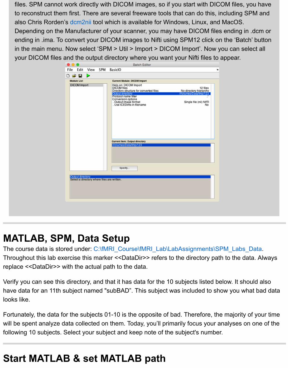
files. SPM cannot work directly with DICOM images, so if you start with DICOM files, you haveto reconstruct them first. There are several freeware tools that can do this, including SPM andalso Chris Rorden’s dcm2nii tool which is available for Windows, Linux, and MacOS.Depending on the Manufacturer of your scanner, you may have DICOM files ending in .dcm orending in .ima. To convert your DICOM images to Nifti using SPM12 click on the ‘Batch’ buttonin the main menu. Now select ‘SPM > Util > Import > DICOM Import’. Now you can select allyour DICOM files and the output directory where you want your Nifti files to appear.

MATLAB, SPM, Data SetupThe course data is stored under: C:\fMRI_Course\fMRI_Lab\LabAssignments\SPM_Labs_Data.Throughout this lab exercise this marker <<DataDir>> refers to the directory path to the data. Alwaysreplace <<DataDir>> with the actual path to the data.

Verify you can see this directory, and that it has data for the 10 subjects listed below. It should alsohave data for an 11th subject named "subBAD”. This subject was included to show you what bad datalooks like.

Fortunately, the data for the subjects 01-10 is the opposite of bad. Therefore, the majority of your timewill be spent analyze data collected on them. Today, you’ll primarily focus your analyses on one of thefollowing 10 subjects. Select your subject and keep note of the subject's number.

Start MATLAB & set MATLAB path

Locate MATLAB under the Start menu and start it (it is also on the desktop).

The first thing you should do after starting MATLAB is to change the working directory to a reasonableplace. In the computer lab you do not have write permissions in the default directory. Use the "..."button at the top of the MATLAB window (depending on the version of MATLAB you’re using, thisbutton may be represented by an open folder icon with a downwards pointing green arrow on it), oruse the "cd" command to change to the <<DataDir>> directory. If you use the cd command you wouldhave to type:

cd <<DataDir>>

Now, add the directory "C:\SPM12" to the path, by either entering "pathtool” in the command window,or by using the "Set path..." button under the "Environment” block in the MATLAB ribbon:

cd C:\SPM12

Click the "Add Folder..." button to select the SPM12 folders.

DO NOT add with subfolders. Click "Close", and save this path in Documents\MATLAB for your futuresessions.

Alternatively you can directly add the folder the path by typing "addpath C:\SPM12”

Check defaultsWhen SPM is first installed it is important to review and set the defaults, found in spm_defaults.m.Navigate to the C:\spm12 directory and open the SPM12 directory. Find the file "spm_defaults.m"and open it by double clicking or by typing "edit spm_defaults.m” (it should open in the MATLAB m-file editor). Remember that if you always have to restart SPM in order to apply your changes.

BOX: Analyze Orientation Defaults If you have the old style Analyze img/hdr pairs you should educate yourself on the flipping ofimages based on spm_flip_analyze_images.m. When first installing SPM it is crucial to set the"flip" default correctly. Find the line with flip in spm_flip_analyze_images.m. A value of 0

indicates that "SPM" Analyze images are expected; such images are often referred to as"Neurological" Analyze. A value of 1 indicates that official Analyze images are expected; theseimages are sometimes called "Radiological". If your lab uses Analyze format, then this valueshould be set once, verfied, then never changed. (The images you’re about to analyze are inthe NIFTI format. Please see the Appendix for more information on NIFTI).

Maximum Memory default: The amount of data acquired during a functional brain scanning session is large. Computers need toanalyze these data in portions and in order to do that, the matlab package SPM processes data in"chunks". The maximum chunk size is determined by the defaults.stats.maxmem setting in thespm_defaults.m file. In the factory, this is set to "2^29" (i.e., 512 MB), which allows SPM to run oneven the most feeble computer.

However the computers you are using in this lab can process larger chunks of information thereforewe increased this limit to 2^30 (i.e., 1 GB). When you are running SPM in your own computer you cansafely set this to as much as half of your computer’s total RAM. So for instance, if you intended to use2 Gigabytes of memory you would type in:

defaults.stats.maxmem = 2^31;

in spm_defaults.m and then save the file.

Now we have set the defaults such that we can begin using SPM. (You may close the editor windowdisplaying spm_defaults.m). Remember that if you always have to restart SPM in order to apply yourchanges.

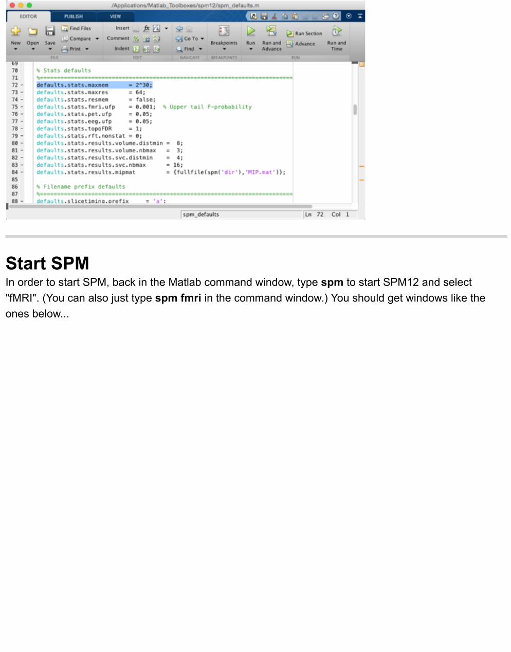
Start SPMIn order to start SPM, back in the Matlab command window, type spm to start SPM12 and select"fMRI". (You can also just type spm fmri in the command window.) You should get windows like theones below...

Selecting files in SPM12 & examining functional dataYou should always examine your functional images to check orientation and to detect any possiblecatastrophic problems. SPM package has tools that make it easy to do this. SPM has a user interface,which allows the user to choose the images that they intend to explore. This is accomplished by thefile selection box, which is brought whenever you try to display images. For those of you not familiarwith SPM, this box has certain features that might be counterintuitive. Let’s walk through the steps:

1. Use the "Display" button to bring up the dialog that will allow you to choose the functional imageyou are intending to explore. The SPM12 select dialog, which is invoked by clicking the displaybutton, shows folders on the left and files on the right. Once you select a file it will show up onthe bottom of the dialog. You may navigate through folders with a *single* click.

2. Now you need to navigate to <<DataDir>> where you will find subject directories named afterthe date of the acquisition and subject's initials (e.g. "sub05"). Functional data are in eachsubject's directory in "func/whyhow/run_01"; "rrun_01.nii" is the data after motion correction aswas covered in lecture. Note that these are 4D NIFTI images, with all of the acquired 3D imagesin one file.

3. The select interface initially assumes that all files are 3D Analyze files, i.e., that they onlycontain a single volume where a volume refers to the signal acquired from the subjects’ brain at

one time point in the experiment. This is reflected in the ",1" after the filename. Since we areintending to display image number 100 we need to be able to see all the volumes. In order to dothis we need to change the volume specification to "1:300” in order to see all the volumes inthe directory (as displayed in the screenshots below). Now you can scroll down until you findrrun_01.nii,100. Click on the filename so that it appears in the bottommost window, as in thescreenshot below. Then click Done. When you change the volume specification SPM willautomatically expand all files in the directory. To filer only the files that we are interested in, wecan make use of regular expressions (see box Regular Expressions).

BOX: select images dialog If you accidentally select a file (removing from the list on the right, moving it to the list on thebottom) you can de-select it by clicking on it. Unfortunately, that file does not re-appear in thelist on the right. To refresh the list of files on the right, hit the "Filt” button.

BOX: Analyze Orientation Defaults Regular expressions (regex) are special text strings that define a search pattern. Thesepatterns can help you select for example only those files that contain a certain string, or thatstart or end with a certain string. A short overview on regular expressions can be found HERE.In short: when you open a SPM dialog you will see .* already filled out in the search box. Thismeans ‘show all files’. If you replace .* with a single character in the search box it will match allfiles that contain that character. Regex distinguishes between upper and lower case

characters. If you want to select only files that start with a certain pattern you can add a ‘^’before your query. For example: ‘^w’ will filer all files that start with w. If you want to select allfiles that start with ‘w’ and also contain ‘subject_001’, you can enter ‘^w.*subject_001’. The ‘.*’in the middle will allow other characters between the leading ‘w’ and the following‘subject_001’. Regex have many other sophisticated features that are worth looking into.

Using the SPM Display Dialog Now that the display dialog is open you may click around the orthogonal views of the brain (coronal,sagittal, transverse) in order to explore your images.

Try to answer the following questions:

1. What is the voxel size?2. What are the image dimensions?3. What are typical gray matter intensity values?4. On the lower right hand side of the display dialog you may see the kind of interpolation being

used in visualizing the images. Trilinear interpolation is default. First select Nearest Neighborinterpolation and explore the image. Next select Sinc interpolation and again explore the image. a. Which interpolation do you prefer? b. Why? It doesn’t really change anything substantial.

Compare the functional data to the anatomical dataNow that we have explored the functional image of our choice we should make sure that thefunctional images are in the same space as the low-resolution T2 overlay anatomical images that we

have acquired for each subject. These data are found within each subject’s directory:

i.e. <<DataDir>>\sub05\anatomy

Anatomical low-resolution T2 overlay images (not to be confused with the high-resolution T1anatomical images) in general have smaller in-plane voxels (i.e. greater in-plane resolution) but theyhave the same number of slices with the same spatial location. In order to ensure that functional andanatomical images are lined up (coregistered) we need to check their registration. This isaccomplished by clicking the Check Reg button in the SPM dialog

Click the Check Reg button:

1. Note that the Check Reg button brings up a dialog box that is very similar to the one you haveseen in the Display example in the previous section. One of the differences is that the CheckReg dialog will allow you to choose multiple files for you to be able to check theircoregistration.

Since we are checking the registration of the anatomical (anat_lores.nii) and functional (e.g.,rrun_01.nii,100) we need to make sure that they are both present in the "Images To Display”portion of the dialog box. To do this, navigate to the anatomical subdirectory mentioned aboveand select anat_lores.nii and then navigate back to the directory in which functional imagesreside and select rrun_01.nii,100. Then click Done.

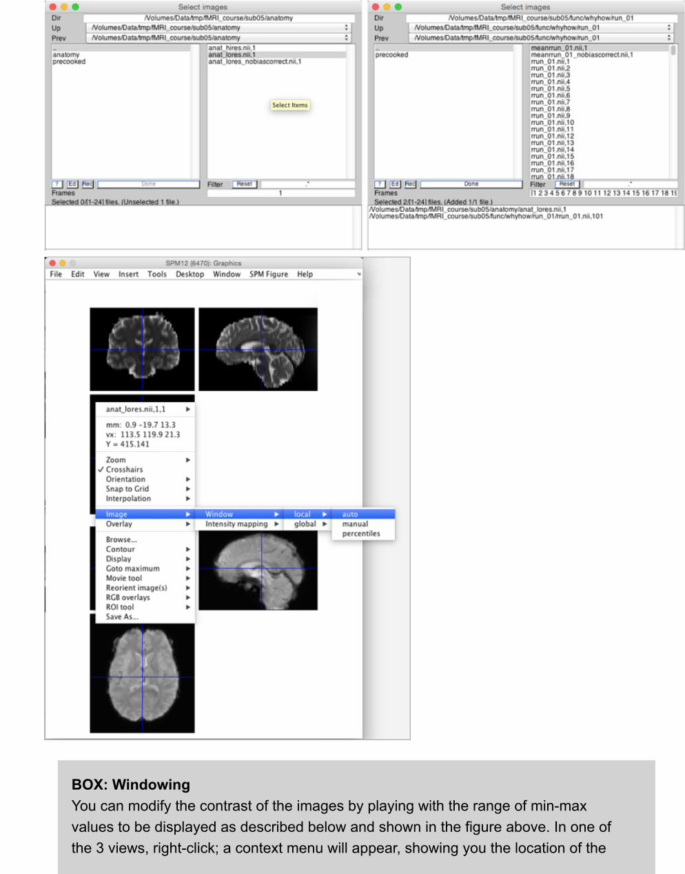
BOX: WindowingYou can modify the contrast of the images by playing with the range of min-maxvalues to be displayed as described below and shown in the figure above. In one ofthe 3 views, right-click; a context menu will appear, showing you the location of the

cursor and the intensity of the voxel under the cursor (shown as "Y = 415.141", forexample). From the context menu, select:

Image:Window:local:manual

and enter a new minimum and maximum value. Try 0 and 110% of typical values. Forexample, if most of the brain is around intensity 1000, a good maximum is probably1050 and you would enter "0 1050".

2. Note that now you see both the anatomical and functional images in the same window. If youclick around one, note that the crosshair in the other will also move. This is how one checkswhether two images are correctly coregistered. Specifically, there are certain landmarks in thebrain, which are used to ensure that all parts of the brain are correctly coregistered.

Explore the pair of images, making sure to compare the following anatomical regions:

i. Frontal poleii. Occipital (posterior) poleiii. Left & Right sides (e.g. superior temporal gyrus)iv. Corpus callosum:

a. Most anteriorb. Most superiorc. Most posterior extent

Do the functional and structural line up well? If not, how so?

Explore the regions of signal loss as we described in the morning lecture. This usuallyhappens in the temporal poles and the orbitofrontal cortex.

Temporal Poles Orbitofrontal Cortex

On the anatomical image, go to the medial orbitofrontal cortex and look at the sagittal image;click on the coronal or axial until you have nice view on the sagittal image---that is, not right onthe mid-sagittal plane (to avoid the cerebral fissure), but just off mid-sagittal.

Now click around on the sagittal view, keeping an eye on the axial view, and carefully comparethe T2 and the functional.

Similarly, find the signal void in the temporal lobe (due to the ear canal). Observe cortex visiblein the T2 anatomical image not visible in functional (T2*) image.

When we get thresholded activation maps, we typically overlay them on the structural imagessince they have more anatomical detail. But why should we *also* check localization ofactivation on the functionals?

BOX: Despiking Brief global signal change due to artifacts (such as noise spikes during acquisition leading to"white pixel” effects) can be detrimental to functional MRI studies. Further, the presence ofthese artifacts can reduce the efficacy of other preprocessing steps; e.g. motion correction.Thus, detection and correction for these artifacts is important in functional MRI.

Typical despiking routines will look for significant deviation from the average signal intensity(such as flagging points that fall 3 standard deviations from the mean), then replace thosepoints with the average of the nearest non-corrupted timepoints. This can be done in k-space(typically called "despiking”) or in image space (sometimes called "scrubbing”). Oneadvantage of doing it in k-space is that it is prior to reconstruction and other processing steps,and can remove a smaller amount of degrees of freedom (one k-space timepoint versus oneimage timepoint). In UM spiral imaging data, we apply despiking in the k-space data beforeimage reconstruction.

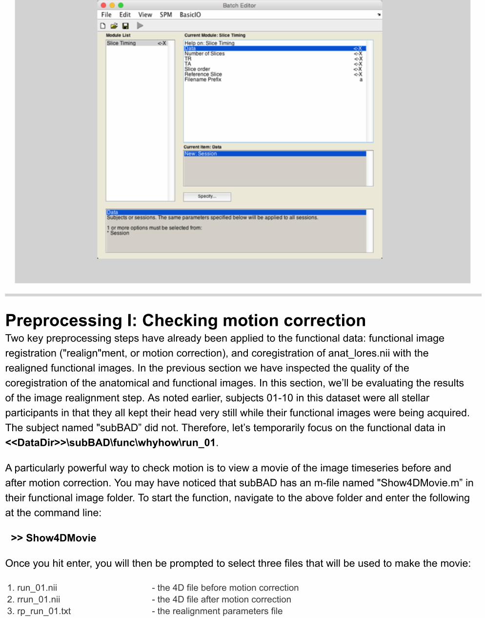
BOX: Slice time correction The 3D volumes (TR’s) in fMRI that form 4D datasets are commonly collected in 2D slices.This results in a temporal offset between slices, meaning that one Because timing is importantfor functional MRI we want to adjust the slice timing trough temporal interpolation, so that allslices show the activation that the would have shown if they would have been collected at thesame time. SPM has a build in tool that can be found on the main menu (‘Slice timing’). Thefirst thing you need to do is click ‘Data’, specify ‘new session’ and select all 3D images in yourdata set. In SPM’s slice timing tool you further have to enter the number of slices in each 3Dimage, the TR (acquisition duration of each 3D volume), the TA (TR-(TR/number of slices), theslice order (see THIS explanation by Chris Rorden), and a reference slice. For a referenceslice, often the middle slice that was collected is selected to ensure that the maximuminterpolation is minimized. After everything has been filled out you can click on the play buttonto obtain slice time corrected 4D images. The data that you will be working with today isalready corrected for slice timing.

Preprocessing I: Checking motion correctionTwo key preprocessing steps have already been applied to the functional data: functional imageregistration ("realign"ment, or motion correction), and coregistration of anat_lores.nii with therealigned functional images. In the previous section we have inspected the quality of thecoregistration of the anatomical and functional images. In this section, we’ll be evaluating the resultsof the image realignment step. As noted earlier, subjects 01-10 in this dataset were all stellarparticipants in that they all kept their head very still while their functional images were being acquired.The subject named "subBAD” did not. Therefore, let’s temporarily focus on the functional data in<<DataDir>>\subBAD\func\whyhow\run_01.

A particularly powerful way to check motion is to view a movie of the image timeseries before andafter motion correction. You may have noticed that subBAD has an m-file named "Show4DMovie.m” intheir functional image folder. To start the function, navigate to the above folder and enter the followingat the command line:

>> Show4DMovie

Once you hit enter, you will then be prompted to select three files that will be used to make the movie:

1. run_01.nii - the 4D file before motion correction2. rrun_01.nii - the 4D file after motion correction3. rp_run_01.txt - the realignment parameters file

Once the program loads the data, the movie will start in a figure window like the one shown below:

The top two images show the timeseries before and after motion correction from the samesagittally oriented slice.The bottom two images plot the timeseries of the estimated head translations (in mm) andestimated head rotations (in degrees).The position of the moving vertical lines corresponds to the number of the image being show

above.

Once the movie finishes, you should see a prompt at the MATLAB command window asking you ifyou’d like to re-play. Once you’re satisfied, answer the questions on the following page.

Try to answer the following questions:

1. On which dimension of translation did subBAD move most?2. On which axis of rotation did subBAD move most?3. Can you see any residual head motion in the image time series after motion correction?4. Should subBAD be excluded from the study? Why or why not?

Preprocessing II: CoregistrationSPM's "Coregister" facility is used for registering different types of images from the same subject (it isa "intermodality, intrasubject" registration). To use it you must specify a "Reference" image, whichdoes not move, and a "Source" image, which is transformed to match the reference.

Historical Note:Beginning with SPM2, the rigid body transformation was recorded in an auxiliary .matfile named like the source image. With either SPM2, SPM5, SPM8 or SPM12 it is not necessary towrite out the transformed image (the Source transformed into the space of the Reference), though it issometimes convenient to do so.

Before coregistering the low- and high- resolution structural images we need to (I) make sure the twoimages are in the same orientation and not too far from one another, and (II) correct for intensityinhomogeneities in the high-resolution T1 image.

1. First see how close the anat_lores and anat_hires images are to start with. What button do youuse to view more than one image?

Multiple images are displayed in the space of the first image. If they are not previouslyregistered this simply means that their origins are lined up.

Neither image has had their origin set. The default origin is the center of the volume. To seethe specific voxel that is defined as the origin, use 'Display' and look in the lower right panel.

2. If the images were very out of register we could try to get the images closer by manuallysetting the origin to the Anterior Commissure (AC).

A. Here is a diagram of how to find the AC on the midsagittal plane:

B. Now use the Display button to view the anat_lores image and find the location, as bestas possible, of the AC. You should be able to see it on the axial slice.

Hint: Once you are close, it helps to "zoom in". In the display facility, click on the "FullVolume" pop-up menu; select "80x80x80 mm" - What is the location of anat_lores's AC in voxels?

C. Use the Display button view the T1 image and locate the AC, as best as possible. - What is the location of T1's AC in voxels? - What is the location of T1's AC in mm?

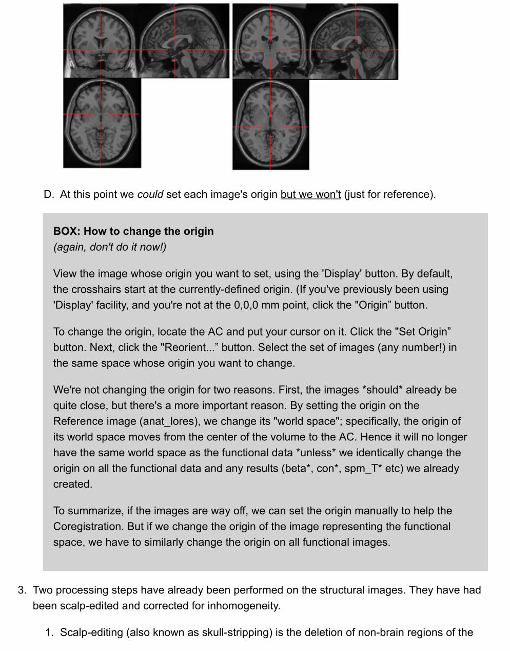
D. At this point we could set each image's origin but we won't (just for reference).

BOX: How to change the origin(again, don't do it now!)

View the image whose origin you want to set, using the 'Display' button. By default,the crosshairs start at the currently-defined origin. (If you've previously been using'Display' facility, and you're not at the 0,0,0 mm point, click the "Origin” button.

To change the origin, locate the AC and put your cursor on it. Click the "Set Origin”button. Next, click the "Reorient...” button. Select the set of images (any number!) inthe same space whose origin you want to change.

We're not changing the origin for two reasons. First, the images *should* already bequite close, but there's a more important reason. By setting the origin on theReference image (anat_lores), we change its "world space"; specifically, the origin ofits world space moves from the center of the volume to the AC. Hence it will no longerhave the same world space as the functional data *unless* we identically change theorigin on all the functional data and any results (beta*, con*, spm_T* etc) we alreadycreated.

To summarize, if the images are way off, we can set the origin manually to help theCoregistration. But if we change the origin of the image representing the functionalspace, we have to similarly change the origin on all functional images.

3. Two processing steps have already been performed on the structural images. They have hadbeen scalp-edited and corrected for inhomogeneity.

1. Scalp-editing (also known as skull-stripping) is the deletion of non-brain regions of the

image volume, i.e., the scalp and skull. Since this extraneous information can throw offsubsequent preprocessing the images have been scalped-edited with the BrainExtraction Tool (BET) from the FMRIB Software Library (FSL).

2. Correction for inhomogeneity (also known as bias correction) accounts for the fact thatanatomical images obtained with high-field magnets (> 2T), tend to be brighter in thecenter of the field of view than at the edge. This inhomogeneity can throw-off subsequentpreprocessing, especially segmentation. Therefore, the images have been corrected forinhomogeneity. The uncorrected images have "_nobiascorrect" appended to them. Seesidebar for further details.

4. Use Check Reg to compare anat_lores.nii to anat_lores_nobiascorrect.nii.

1. Can you see the greater intensity in the center of the uncorrected image?2. Does the corrected image look better?

BOX: Inhomogeneity CorrectionImages were corrected for inhomogeneity using two SPM8 functions. The first,spm_bias_estimate.m, estimates the image inhomogeneity. This estimate is saved ina "bias field” matrix that is used to correct for inhomogeneity using the secondfunction, spm_bias_apply.m. In the following example, these functions are used tocorrect anat_lores.nii. It assumes that you are working in your subject’s anatomicaldirectory:

>> biasfield = spm_bias_estimate('anat_lores_nobiascorrect.nii'); >> spm_bias_apply('anat_lores.nii', biasfield);

If successful, this should yield a bias corrected version of the image with "m”prepended to the name (in this case, "manat_lores.nii”).

5. You will now "Coregister" the high-resolution anatomical image (anat_hires) to the low-resolution anatomical image (anat_lores). The anat_lores image has the same space as thefunctionals, and hence this coregistration will set anat_hires' world space to correspond to thefunctionals. Make sure you know answers to the following:

A. What is your "Reference" image?B. What is your "Source" image?C. Click on the Coregister button. In the Batch Editor select

New Coreg: Estimatei. Double click Coreg: Estimate, thenii. Set the Reference and Source images you identified above.iii. Now "Run" the job to perform the coregistration.

The transformation parameters are written into the NIFTI file of the source imageanat_hires (if a file initially has an Analyze header, it is silently converted to a NIFTIheader). Please see the Appendix for more information on NIFTI. This action sets theworld space of anat_hires to match that of anat_lores. Given that the world space ofanat_lores already matched that of the functional images, this means that theanat_hires is now in the world space of the functional images.

D. Note: changes in world spaces."Display" anat_lores.nii and use the "World Space"/"Voxel Space" pop-up buttonto change between the two spaces.Does the image move as you flip between the two spaces? If so, do youunderstand why?"Display" anat_hires.nii and do the same again.Does the image move as you flip between the two spaces?Why do the images move between spaces?

E. Check the success of the Coregistration.

Use check reg to check the registration. Check the points mentioned before:i. Frontal poleii. Occipital (posterior) poleiii. Left & Right sides (e.g superior temporal gyrus)iv. Corpus Callosum

a. Most anteriorb. Most superiorc. Most posterior extent

v. Trace the sulci

Has the coregistration succeeded?

Preprocessing III: Spatial NormalizationSpatial Normalization is used for intersubject (between subject) registration. It is essential forperforming intersubject analyses for determining Talairach/MNI coordinates of activation foci.

While the "Normalise" button can accept any kind of image (T1, T2, etc), to register your subject intothe standard atlas space, it is important to use the highest resolution structural data.

1. For us, that is which image?

(Check your answer before continuing on!)

Spatial normalization (or, with a British spelling, normalisation) takes three types of images

i. Image to Align These are the high resolution anatomical images from which the spatial transformation isdetermined. Typically you only specify *one* such image per subject.

ii. Images to Write (normalised) These are other images *with* *the* *same* *world* *space* as image (i) above. Typicalexamples would be statistic or contrast images, or whole set of ra* functional images.

iii. Tissue probability map The normalization parameters are obtained through segmentation (see box: SPM12normalization). The tissue probability map (TMP.nii) is a 4D image that contains a totalof 6 3D images of the following modalities: gray matter, white matter, cerebrospinalfluid, fat tissue, bone tissue, and air. The atlas space of this TPM defines the space thatyou warp your images to. In short: the TPM defines the world space of your normalizedimages. In SPM12, the world space of the standard TPM is MNI152.

It produces a "y_*.nii" deformation field image (see box: SPM12 normalization), whichrecords the nonlinear transformation *from* the *world* *space* of image (i) *to* the

atlas space.

2. Now that we have coregistered, what does the world space of anat_hires correspond to?

3. Thus if we spatially normalize anat_hires the resulting anat_hires_sn.mat file will not just begood for anat_hires, but also for ...?

Click 'Normalise' to start the spatial normalization process. Select "Normalise: Estimate &Write" in the drop-down menu, find the "Data” item in the hierarchy and click "New Subject" (fornow, just do one subject). Under "Subject”, for "Image to Align", select anat_hires.nii, thehomogeneity-corrected, scalp-edited, hi-res anatomical image that is now in the space of thefunctionals. For "Images to write", select again anat_hires.nii.

BOX: SPM12 NormalizationNormalization consists of several steps which can generally be divided into an initiallinear (affine) part that uses 12 degrees of freedom (translations, rotations, shearing,and stretching) and a consecutive non-linear component.

In SPM12 spatial normalization is no longer based on minimizing the mean squareddifference between a template and a warped version of the image. Instead, it is nowdone via segmentation, as this provides more flexibility. I.e., a nonlinear deformationfield is estimated that best overlays the atlas on the individual subjects’ image. Theolder way of spatially normalizing images that was used in SPM8 and older versions isstill available via the "Old Normalise" Tool. However, the aim is to try to simplify SPMand eventually remove the older and less effective routines.

BOX: Deformation fieldsDuring the non-linear transformation, for each voxel it is calculated how it should moveand shrink or expand to fit the template image. This information is stored in thedeformation field (y_*.nii) instead of sn.mat files which was the case in previous SPMversions. The current format allows much more precise alignment. It contains threeimage volumes encoding the x, y and z coordinates (in mm) of where each voxelmaps to.

The images below show an example of 1 3D volume of the flowfield that encodes forthe x (coronal; left image) and y (sagittal; right image) deformations. The right imageshows the deformation field overlaid on the high-resolution anatomical image.

Click "Run” to run the job, after a short while it will finish. This will create a y_anat_hires_.niiand reslice the requested file, creating a wanat_hires.nii.

Check the success of the registration, comparing the normalized image (wanat_hires.nii) to theunsmoothed version of the template image that is avg152T1.nii in the SPM12\canonicaldirectory.

4. Using the landmarks suggested above, has the spatial normalization succeeded?

5. Above, we noted that the "Estimation” part of "Estimate & Write” saves the nonlineartransformation necessary for normalizing any image that is in the same space as (or co-registered with) the anat_hires.nii. The file it saves should be located in the same directory asanat_hires.nii, and should be named y_anat_hires.nii. Now, we can use this file to normalize thefunctional images. To do so, first click ‘Normalise’ as before. Given that we’ve already estimatedthe nonlinear transformation (and have the y_*.nii file to go along with it), we should select"Normalise: Write” in the menu. Find the "Data” item in the hierarchy and click "New Subject" asbefore. Under "Subject”, for "Deformation Field", select the y_anat_hires.nii we just estimated.For "Images to write", you’ll want to select all 300 functional images. Navigate to that subject’s"func/run_01” directory and change the volume specification to 1:300 as before. Then, firstselect rrun_01.nii, 1, and then scroll down and shift-select rrun_01.nii,300 to grab all 300images. The select dialog should report "Selected 300 files". (If you select the wrong files right-click in the bottom selected file box, and select "Unselect All".)

6. Save and run your job. Given that this job will write a new 4D file, it will take a couple minutesto finish. When it does finish, you should have a file named "wrrun_01.nii” in the same directoryas your original 4D functional file. Use the "Check Reg” function to visually examine the qualityof the registration between the normalized anatomical (wanat_hires.nii) and one of thenormalized functionals (e.g., wrrun_01.nii,300).

Preprocessing IV: SmoothingThe only preprocessing step left to do for an intrasubject analysis is spatial smoothing (we'll use8mm). This is done in order to increase signal to noise ratio (SNR) and the ability of statisticaltechniques to detect true and task related changes in the signal. We’ll use the Batch Editor moduleSpatial:Smooth to implement this.

1. Click the "Smooth" button in the top-left window. The graphics window now shows a 4-panelinterface. The upper left shows the hierarchy of the current job; the bottom panel displays helpmessages (these are often quite helpful!); the right column of panels are used to input newvalues and review current values in the job specification. The top-left panel should show:Smooth <-X The "<-X" marker indicates that there are required options that have not beenspecified. As long as there are any "<-X " markers present the job cannot be run (notice thatthe Run button is grayed-out)).

2. If the window with the title "Current Module” is empty, double click "Smooth <-X ". Six sub-options appear. The first item is SPM’s built in help on the topic of smoothing. The seconditem, "Images to Smooth”, since it bears the "<-X " marker must be set. The other four alreadyhave default values set.

3. Select "Images to Smooth" by single-clicking it. Then in the lower right, single-click "SelectFiles". Alternatively, you can double click "Images to Smooth”. Once you have the dialog open,select all 300 normalised images within your freshly written "wrrun_01.nii” 4D file. Theselection procedure is the same as in the "Normalise: Write” job described above, but makesure you’re selecting the 4D file with "w” prepended to it. Once you’re sure you’ve selected all300 normalised images, click ‘Done’, and confirm that the correct files were selected (asshown in the 2nd box in the right-hand column of the Batch Editor).

4. Set smoothing. The interface allows us to specify things such as the width of the filter. Sincewe accomplish filter/smoothing by simply convolving our signal with a three dimensionalGaussian function we can specify the extent of smoothing by using the full width at halfmaximum (FWHM) of the Gaussian Kernel. This can be done by clicking "FWHM". Note that adefault smoothing of "8 8 8" has already be set, so there is no need to change anything.

5. Now it is time to start the job. You can do this by clicking the green filled triangle button or byselecting "Run Batch” under the file drop-down menu. (Note that at this point we could haveclicked File> Save Batch to save the job in .mat, .m or .xml formats. For such a simple job,there is no point in saving the job.) You will notice that the window on the lower left hand sidewill display a progress bar.

6. Smoothing creates images with a "s" prefix. Use "Check Reg" to compare the first and lastimage (1 and 300) from both the unsmoothed (wrrun*) and smoothed (swrrun*) 4D image files.(This will ensure that you smoothed all the images, and give you a visual feel for the impact of8mm smoothing).

APPENDIX

Notes on preprocessingThere are several ways to check the quality of preprocessing stages in fMRI. You can check most ofthem using spm_check_registration ("Check Reg” in the GUI). If you or someone in your lab can dosome scripting, it may be a good idea to automatically generate images that show the following foreach subject and save them in an electronic "log book.” Here’s a suggested list:

1. Do the functional images appear coregistered with the anatomical image (overlay) you willnormalize to the template?

2. Are the anatomical images you will normalize roughly in alignment with the template?3. Do the normalized anatomical images seem closely matched to the template?4. Do the normalized functional images seem to be in reasonable alignment with the template?

BOX: NIFTI (Neuroimaging Informatics Technology Initiative)The purpose of the Neuroimaging Informatics Technology Initiative is to support service,

training and research to develop and enhance the utility of informatics tools used inneuroimaging, with a focus on functional magnetic resonance imaging (fMRI).

NIFTI is jointly sponsored by National Institutes of Mental Health (NIMH) and the NationalInstitutes of Neurological Disorders and Stroke (NINDS) which are part of the NationalInstitutes of Health (NIH) and Department of Health and Human Services (DHHS). The DataFormat Working Group (DFWG) of NIFTI is in charge of coming up with a technical solutionto the problem of multiple data formats used in fMRI research. The NIFTI header that werefer to in this tutorial is the supplemental information that is placed at the beginning of thefMRI data. This header has the parameter settings for aspects of the data such as voxel size,affine transformation and number of slices. When two images are coregistered, the rigid bodytransformation that maps one image to the other is stored as quaternions, which are shortforms of rotation/scaling/translation/shearing matrices, in the NIFTI header. A schematicdescription of how this information is used is included below.

BOX: Batch Job BasicsIt is possible to use SPM commands and run batch jobs without having to use the graphic

user interface. Experience with this will increase your speed and power in processing yourdata.

The following code uses the saved normalization job from above.

1. The following commands let you bring up and run the Batch Editor from the commandline in MATLAB.

% brings up Batch Editor in interactive mode spm_jobman('initcfg') spm_jobman('interactive') % You can then create, edit, load, save, and run batch jobs; try loading the normalization batch file

2. Alternatively, you can also load and run batch jobs from the command line.

batchname=spm_select(1,'mat','Select batch file with normalization') load(batchname) spm_jobman('run', matlabbatch)

3. You can also load batch jobs, and use the results in any other spm modules. Thiscode loads the normalization batch file, and brings up the check registration window:

% Select and load batch file batchname=spm_select(1,'mat','Select batch file with normalization');}

load(batchname)}

% Get file names src = matlabbatch{1}.spm.spatial.normalise.estwrite.subj(1).source{1}

template = matlabbatch{1}.spm.spatial.normalise.estwrite.eoptions.template{1}

% Append w to src name to select normalized file [dd, ff, ee] = fileparts(src)

wsrc = fullfile(dd, ['w' ff ee])

% Compare images spm_check_registration(char(template, wsrc));