presentation for bank of italy seminar - banca d'italia · presentation for bank of italy...
TRANSCRIPT

22 September, 2010
Presentation for Bank of Italy Seminar
Structural VARs for Heterogeneous Panels;
With Applications to European Regional Income Dynamics
and International Exchange Rate Dynamics
Peter Pedroni
Williams CollegeMassachusetts, USA

2
Presentation Outline
I. General Overview
II. Details of Methodology
- econometric issues
- nontechnical summary
III. International Exchange Rate Dynamics
- data description
- identification strategy
- empirical results

3
IV. European Regional Income Dynamics
- data description
- identification strategy
- empirical results
VI. Conclusions
- and directions for future research, in macro and regional economics

4
I. General Motivation
Often interested to exploit multi-country or multi-regionaldimensions for panel time series
Literature on nonstationary panels does this
- but focused on long run steady state issues
- unit roots, cointegration, etc.

5
But often interested in short run dynamic issues
- how to regions respond to over time to national and local business cycle variations
- what region specific characteristics determine the shape and size of the responses
- can patterns across countries better help us identify reasons for unusual exchange rate dynamics
Is it possible to exploit panel time series toward this end?

6
If so, need to be careful regarding treatment of threeimportant issues
1. Dynamics likely to be heterogeneous
- if ignore heterogeneity and pool dynamics leads to inconsistent estimation
- estimates do not converge to mean values of heterogeneous parameters
- classic problem of latent heterogeneity in lagged dependent variables
(See Pesaran and Smith, 1995, for review)

7
Background on older “dynamic panel” techniques:
- VARs for homogeneous panels already exist
(See Holz-Eakin, Newey and Rozen, 1988)
- dynamic panel literature (Arellano and Bond, etc) is special cases of homogeneous panel VARs
- but homogeneity assumption almost certainly violated for any aggregrate data
- would imply identical impulse responses in terms of size, shape, duration, etc.
- not appropriate for macro or regional data
8
2. Time series dimension is likely to be short
- want to apply in circumstances when T dimension too short for conventional time series
- need to treat heterogeneous dynamics, but don’t have advantage of superconsistency
Background comparison:
- for nonstationary panel methods dynamics do not need to be well estimated
- do not need to be estimated jointly with long run
- can be treated as nuisance feature in distributions for long run inference
- due to fact that dynamics have only second order impact relative to the long run levels

9
So not obvious that can recognize gains from panels
Solution: Use spatial dimension directly to constructconfidence intervals
- results in relatively tight confidence intervals even with short T
- eliminates need for bootstrapping confidence intervals
- BUT, this brings into focus the next issue:

10
3. Cross sectional dependencies must be accommodated
- countries and regions likely to be interdependent
- if want inferences regarding spatial distribution of responses to be valid need to control for this
- but interdependencies likely to be dynamic
- which brings into focus the next issue:
4. Economic “forcing process” often unobserved
- i.e. most responses of interest are to “structural” economic shocks, not to observables
- need to deal with structural identification
- particularly given that need to accommodate dynamic interdependencies in responses to shocks

11
Solution: Use structural VAR approach so that canidentify orthogonal shocks
- at both local and global level
- and use orthogonality to decompose composite shocks into local versus global shocks
- and thereby allow complex interactions in terms of responses to shocks

1.3 Relationship to other approaches
• Canova and Ciccarelli (2004, 2009)
− Use Bayesian VAR estimation approach
− Allow for time varying coefficients
− Treat cross sectional dependency using fac-
tor model
− Focus on responses to innovations in observ-
ables (not unobserved structural shocks)
− Multi-country application: Response of
other large economies to innovations in U.S.
GDP

• Eickmeier (2009)
− Use classical estimation approach
− Do not allow for time varying coefficients
− Also treat cross sectional dependency using
factor model
− Focus on idiosyncratic responses to com-
mon factor model shocks. Do not do pool
or group responses to idiosyncratic shocks
− Multicountry application: Heterogeneity of
European country responses to European
common shocks.

• This paper
− By contrast emphasizes properties of full
sample distribution of responses to both id-
iosyncratic and common shocks i
− Uses spatial dimension for confidence inter-
vals around group medians.
− Emphasizes identification of structural
shocks
− Treats cross sectional dependency struc-
turally by using restrictions on time effects
to identify common shocks
− Regional application: Explaining patterns
of heterogeneous dynamics.

1.4 Econometric Technique
• Use panel SVAR to decompose responses to dif-
ferent unobserved structural shock
• Also distinguish common versus idiosyncratic
structural shocks
• Allow heterogenous factor loading responses to
common structural shocks
• Compute distributions of dynamic responses
across i dimension
• Relate distributions to observed regional charac-
teristics xi
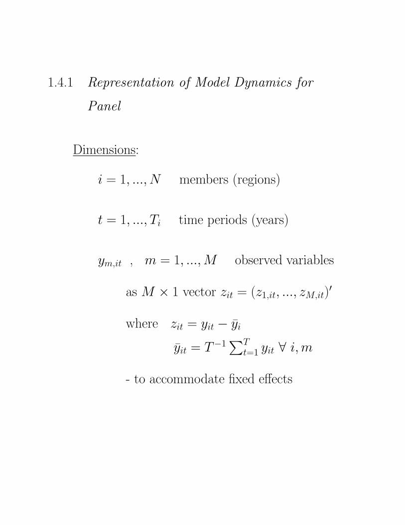
1.4.1 Representation of Model Dynamics for
Panel
Dimensions:
i = 1, ..., N members (regions)
t = 1, ..., Ti time periods (years)
ym,it , m = 1, ..., M observed variables
as M × 1 vector zit = (z1,it, ..., zM,it)′
where zit = yit − yi
yit = T−1∑T
t=1 yit ∀ i,m
- to accommodate fixed effects

Unobserved Shocks:
idiosyncratic shocks:
εm,it , m = 1, ..., M
common shocks:
εm,t , m = 1, ..., Mc , Mc ≤ M
composite shocks:
εm,it , m = 1, ..., M , εit = (ε1,it, ..., εM,it)′
such that:
εm,it = λm,iεm,t + εm,it ∀ i, t, m
E(εm,itεm,t) = 0 ∀ i, t, m
E(εitε′it) = IM×M ∀ i, t
E(εm,it) = E(εm,it) = E(εm,t) = 0 ∀ i, t, m
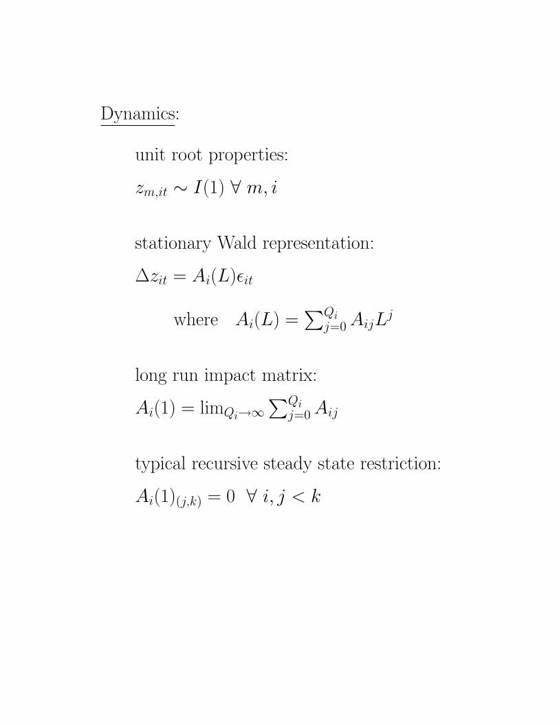
Dynamics:
unit root properties:
zm,it ∼ I(1) ∀ m, i
stationary Wald representation:
∆zit = Ai(L)εit
where Ai(L) =∑Qi
j=0 AijLj
long run impact matrix:
Ai(1) = limQi→∞∑Qi
j=0 Aij
typical recursive steady state restriction:
Ai(1)(j,k) = 0 ∀ i, j < k

1.4.2 Estimation and Inference for Panel
Estimation:
1. Estimate Ri(L)∆zit = µit by OLS ∀i
where Ri(L) = I −∑Pij=1 RijL
j
with Pi chosen by AIC ∀i
2. Compute ∆zt = N−1∑N
i=1 ∆zit ∀t
3. Estimate R(L)∆zt = µt by OLS
where R(L) = I −∑Pj=1 RijL
j
with P chosen by AIC

Structural Identification:
Reduced form MA representation
(for composite shocks):
∆zit = Fi(L)µit,
where Fi(L) = Ri(L)−1 , Fi(0) = 0
So that relates to structural form as:
∆zit = Fi(L)µit = Ai(L)εit,
εit = Ai(0)−1µit
A(L)i = F (L)iAi(0)
A(0)i = R(1)iAi(1)

Orthogonality and arbitrary units
E(εitε′it) = IM×M ∀ i, t
Implies:
For contemporaneous covariance:
E(µitµ′it) = E(A(0)iεitε
′itA(0)′i)
= A(0)iA(0)′i
For long run covariance of µit:
Ωi(1) = E(F (1)iµitµ′itF (1)′i)
= A(1)iA(1)′i

Steady state identifying restriction
Ai(1)(j,k) = 0 ∀ i, j < k
Implies:
Ai(1) = Chol(Ωi(1))
So, for composite shocks:
εit = (Ri(1)Ai(1))−1µit
Ai(L) = Ri(L)−1Ri(1)Ai(1)
where Ai(1) obtained from Cholesky of :
Ωi(1) = (Ri(1)−1)Σi(Ri(1)−1)′
Σi = T−1∑T
t=1 µitµ′it

Similarly, for common shocks:
A(1)(j,k) = 0 ∀ j < k
Implies:
A(1) = Chol(Ω(1))
So that:
εt = (R(1)A(1))−1µt
A(L) = R(L)−1R(1)A(1)
where A(1) obtained from Cholesky of :
Ω(1) = (R(1)−1)Σ(R(1)−1)′
Σ = T−1∑T
t=1 µtµ′t

Decompositions:
Estimate common factor loadings, λm,i, as:
εm,it = λm,iεm,t + εm,it by OLS ∀ i,m
composite variances contributions:
Di,s(k, `) =(∑s−1
j=0 Ai,je(`)e(`)′A′i,j)(`,`)
Ψi,s(k,k)
for a given step s, country i,
for shocks ` = 1, ..., M ,
for variables k = 1, ...M
where Ψi,s =∑s−1
j=0 Ai,jA′i,j
and e(l) is the lth unit vector
common variances contributions:
Di,s(k, `) =(∑s−1
j=0 Aje(`)λiλ′ie(`)
′A′j)(`,`)Ψi,s(k,k)
idiosyncratic variances contributions:
Di,s = Di,s −Di,s

Group inference:
group mean estimates:
DN1s (k, `) = N−1
1
∑N1i=1 DR
i,s(k, `)
for any given variable, k = 1, ..., M ,
shock, ` = 1, ..., M ,
response step, s = 0, ..., Qi,
for any N1 ε N group of countries,
of the decomposition matrices:
DRi,s(k, `) ε Di,s, Di,s, Di,s
standard errors:
σD
N1s (k,`)
=√
N−11
∑N1i=1
(DR
i,s(k, `)−DN1s (k, `)
)2
confidence intervals:
use fractiles from sampling distributions of
DRi,s(k, `)

13
Nontechnical Summary
Step 1: Estimate composite reduced form VARs separately for each member i
Step 2: Apply identification scheme to obtain estimates of composite structural shocks for each member i
Step 3: Use cross sectional averages at each point in time for each variable to extract common effects
Step 4: Estimate common reduced form VAR Step 5: Apply identification scheme to obtain estimates of composite structural shocks for each member i
Step 6: For each member i estimate member specific loading vectors for response to common shocks
Step 7: Use estimated loading vectors to decompose composite shocks into common versus idiosyncratic shocks

14
Step 8: For each member i compute structural impulse responses and variance decompositions for common and idiosyncratic shocks
Step 9: Compute sample distribution across i for each time period of impulse responses and variance decompositions
Step 10. Use sample distribution to compute group mean (or median) responses and decompositions
Step 11. Use sample distribution to compute spatial confidence intervals for responses and decompositions
- in contrast to time series SVARs, do not require bootstrap for confidence intervals
Step 12. Regress heterogeneous responses for given step against vector of observable member
specific characteristics .

360
4. Empirical illustration: Sources of Nominal and Real Exchange Rate Rigidity
Basic idea:
Use identified panel SVAR technique to address puzzle inexchange rate literature
Find that structural identification provides possibleresolution to puzzle
- for pure time series would require considerable data
- with panel approach get tight confidence intervals

1
1.1 Motivation
Real exchange rates notorious for slow adjustment
Conventional explanation:
• Aggregate prices are slow to adjust
• Consistent with sticky price macro models
Early empirical puzzle (Rogoff, 1996, others):
• RER adjustment even slower than P adjustment
• Hard to reconcile with conventional idea

2
Recent twist to puzzle:
(Engle, Morley 2001, Cheung, Lai, Bergman 2004):
• Decompose real e into P and nominal E adjust-
ment
• nominal E adjusts much slower than P
• Appears to contradict conventional explanations

MOTIVATION 3
Engle and Morley (2001):
• 6 countries individually
• state space Kalman filter approach
• with PPP imposed
• estimate speed to close P − P ss, E − Ess gaps
consistent with PPP
• P half-life: 3-6 months , E half-life: 2-15 years
Cheung, Lai, Bergman (2004):
• 5 countries individually
• VECM cointegrated VAR approach
• with PPP imposed
• estimate speeds for P and E to close PPP gap
• P half-life: 1 -2 years, E half-life: 3-6 years

4
Why might central banks care about this puzzle?
Puzzle impacts logic of one classic argument for float-
ing exchange rates:
• If trade sector important, may want to minimize
real e fluctuations
• If believe real e often mean reverting in response
to shocks, want quick return to ”parity”
• If P adjustment is slow and sticky, then need
nominal E to be able to do the adjusting
• But if E adjustment slow (possibly even slower
than P) destroys this argument

MOTIVATION 5
Empirical Question: Can structural panel time series
approach contribute toward resolving these puzzles?
Expect relative speeds to be sensitive to shock type
Begin agnostically:
• Initially use simple sticky price open economy
framework for guidance
• Then consider possible refinements and deeper
implications

6
Empirical Strategy:
1. Work with panel of countries
• use group mean dynamics
• allows one to establish patterns in dynamic
distributions
• while allowing heterogeneous dynamics
2. Do not impose long run PPP
• Consider that some shocks may adhere to
PPP (i.e. long run neutral on real e)
• Others may not (i.e. induce permanent real
e movement)

MOTIVATION 7
Regarding long run PPP testing:
unit root tests for e often problematic
both time series and panel versions
Used new test here:
Pedroni,Vogelsang,Wagner,Westerlund (2008)
• untruncated kernel approach
• only test that retains power with short T
when have incidental deterministic trends
• robust to any form of cross sectional depen-
dence
• does not require any choice of lag or band-
width truncation
Clearly rejects unconditional PPP in this sample
• both without and with incidental trends
(e.g. Balassa-Samuelson version)

8
3. Consider implications of long run P neutrality
• some shocks potentially neutral on P for
small open economies with flexible E.
(e.g. real AD shocks that induce short run
e response to maintain real interest parity
may appear neutral on P - details later)
(e.g. supply shocks accommodated with
procyclic monetary response may also ap-
pear neutral on P - details later)
• Other shocks may not be neutral on P
(e.g. nominal shocks, or unaccommodated
supply shocks)

MOTIVATION 9
4. Distinguish common vs. idiosyncratic shocks
• Expected to have very different dynamic re-
sponses
(e.g. common versus idiosyncratic shocks
that are non-neutral on P have very differ-
ent implications for E)

10
1.2 Data
E : log bilateral U.S. nominal exchange rates
P : log local CPI , P∗ : log U.S. CPI
e: computed log real exchange rates
log e = log E + log P − log P∗
(CPI, FX rebased to 1995 for conformity)
time span: Monthly, Jan 1980 - Dec 1998
countries: Industrial (N = 20, T = 228)

Var Decomps to shocks neutral on RER vs. non-neutral on RERRecursive (RER,FX) identification
Summary: Most FX (and RER) variation is due to shocks that are non-neutral on FX.
% variance of RER due to idiosyncratic non-neutral shocks
10 20 30 40 50 60 70 80 90 100 110 1200.800
0.825
0.850
0.875
0.900
% variance of RER due to common non-neutral shocks
10 20 30 40 50 60 70 80 90 100 110 1200.04
0.06
0.08
0.10
0.12
0.14
0.16
% variance of RER due to idiosyncratic neutral shocks
10 20 30 40 50 60 70 80 90 100 110 1200.000
0.025
0.050
0.075
0.100
0.125
% variance of RER due to common neutral shocks
10 20 30 40 50 60 70 80 90 100 110 1200.000
0.002
0.004
0.006
0.008
0.010
0.012
% variance of FX due to idiosyncratic non-neutral shocks
10 20 30 40 50 60 70 80 90 100 110 1200.780.800.820.840.860.880.900.920.940.96
% variance of FX due to common non-neutral shocks
10 20 30 40 50 60 70 80 90 100 110 1200.00
0.01
0.02
0.03
0.04
0.05
0.06
% variance of FX due to idiosyncratic neutral shocks
10 20 30 40 50 60 70 80 90 100 110 120-0.025
0.000
0.025
0.050
0.075
0.100
0.125
0.150
0.175
% variance of FX due to common neutral shocks
10 20 30 40 50 60 70 80 90 100 110 1200.00
0.01
0.02
0.03
0.04
0.05
0.06

Var Decomps to shocks neutral on CPI vs. non-neutral on CPIRecursive (CPI,RER) identification
. . . . . . . . . Summary: Most RER variation is due to shocks that are neutral on CPI.
% variance of CPI due to idiosyncratic non-neutral shocks
10 20 30 40 50 60 70 80 90 100 110 1200.10.20.30.40.50.60.70.80.91.0
% variance of CPI due to common non-neutral shocks
10 20 30 40 50 60 70 80 90 100 110 1200.00.10.20.30.40.50.60.70.80.9
% variance of CPI due to idiosyncratic neutral shocks
10 20 30 40 50 60 70 80 90 100 110 120-0.05
0.00
0.05
0.10
0.15
0.20
0.25
% variance of CPI due to common neutral shocks
10 20 30 40 50 60 70 80 90 100 110 1200.00
0.01
0.02
0.03
0.04
0.05
% variance of RER due to idiosyncratic non-neutral shocks
10 20 30 40 50 60 70 80 90 100 110 1200.000.050.100.150.200.250.300.350.400.45
% variance of RER due to common non-neutral shocks
10 20 30 40 50 60 70 80 90 100 110 1200.000000
0.000025
0.000050
0.000075
0.000100
0.000125
0.000150
% variance of RER due to idiosyncratic neutral shocks
10 20 30 40 50 60 70 80 90 100 110 1200.40
0.45
0.50
0.55
0.60
0.65
0.70
0.75
0.80
% variance of RER due to common neutral shocks
10 20 30 40 50 60 70 80 90 100 110 1200.100
0.125
0.150
0.175
0.200
0.225
0.250
0.275
0.300

Imp Responses to shocks neutral on RER vs. non-neutral on RERRecursive (RER,FX) identification
. . . . Half-lives (months): . . . RER: 25 ( 4 , 25 ) , . . . FX: 2 ( 3 , 2 ) , . . . CPI: 13 ( 32 , 13 ) . . . .
response of RER to idiosyncratic neutral shocks
10 20 30 40 50 60 70 80 90 100 110 120-0.0050
0.0000
0.0050
0.0100
0.0150
response of FX to idiosyncratic neutral shocks
10 20 30 40 50 60 70 80 90 100 110 120-0.0025
0.0025
0.0075
0.0125
0.0175
response of CPI to idiosyncratic neutral shocks
10 20 30 40 50 60 70 80 90 100 110 120-0.0200-0.0175-0.0150-0.0125-0.0100-0.0075-0.0050-0.0025

Imp Responses to shocks neutral on RER vs. non-neutral on RERRecursive (RER,FX) identification
. . . . Half-lives (months): . . . RER: 2 ( 2 , 3 ) , . . . FX: 2 ( 2 , 3 ) , . . . CPI: 4 ( 12 , 2 ) . . . .
response of RER to idiosyncratic non-neutral shocks
10 20 30 40 50 60 70 80 90 100 110 1200.0225
0.0275
0.0325
0.0375
0.0425
response of FX to idiosyncratic non-neutral shocks
10 20 30 40 50 60 70 80 90 100 110 1200.0150.0200.0250.0300.0350.0400.0450.050
response of CPI to idiosyncratic non-neutral shocks
10 20 30 40 50 60 70 80 90 100 110 120-0.004-0.003-0.002-0.0010.0000.0010.0020.003

Imp Responses to shocks neutral on CPI vs. non-neutral on CPIRecursive (CPI,RER) identification
. . . . Half-lives (months): . . . CPI: 4 ( 3 , 12 ) , . . . RER: 2 ( 2 , 3 ) , . . . FX: 2 ( 2 , 3 ) . . . .
response of CPI to idiosyncratic neutral shocks
10 20 30 40 50 60 70 80 90 100 110 120-0.00050
0.00000
0.00050
0.00100
0.00150
response of RER to idiosyncratic neutral shocks
10 20 30 40 50 60 70 80 90 100 110 1200.020
0.025
0.030
0.035
0.040
0.045
response of FX to idiosyncratic neutral shocks
10 20 30 40 50 60 70 80 90 100 110 1200.0150.0200.0250.0300.0350.0400.045

Imp Responses to shocks neutral on CPI vs. non-neutral on CPIRecursive (CPI,RER) identification
. . . . Half-lives (months): . . . CPI: 32 ( 29 , 26 ) , . . . RER: 10 ( 22 , 31 ) , . . . FX: 28 ( 23 , 26 ) . . .
response of CPI to idiosyncratic non-neutral shocks
10 20 30 40 50 60 70 80 90 100 110 1200.0000
0.0050
0.0100
0.0150
0.0200
response of RER to idiosyncratic non-neutral shocks
10 20 30 40 50 60 70 80 90 100 110 120-0.040
-0.030
-0.020
-0.010
0.000
response of FX to idiosyncratic non-neutral shocks
10 20 30 40 50 60 70 80 90 100 110 120-0.06-0.05-0.04-0.03-0.02-0.010.00

20
1.4 Summary of Results
1. Most of variance in nominal E and real e is due
to shocks that are:
a. long run non-neutral on e,
b. and long run neutral on P .
2. For shocks that are neutral on real e:
a. real e adjustment is slow (25 months)
b. P adjustment is moderate (13 months)
c. nominal E adjustment is fast (2 months)
3. For shocks that are non-neutral on real e:
a. real e adjustment is fast (2 months)
b. P adjustment is fast (4 months)
c. nominal E adjustment is fast (2 months)

SUMMARY OF RESULTS 21
4. For shocks that are neutral on P :
a. real e adjustment is fast (2 months)
b. P adjustment is fast (4 months)
c. nominal E adjustment is fast (2 months)
5. For shocks that are non-neutral on P :
a. real e adjustment is moderate (10 months)
b. P adjustment is slow (32 months)
c. nominal E adjustment is slow (28 months)

Interpreting the Results Structurally
Responses:shock real e P nom E %var of enominal: slow moderate fast smallreal AD: fast fast-small fast largeLRAS: moderate slow slow smallAS+M: fast fast-small fast large
These patterns should seem very familiar!
... How familiar? ...

Nominal Shocks (M ↑)
A => B short run (a.k.a. “fast”) before any P adjustment B => C long run (a.k.a. “slow”) after P fully adjusts
Results: Long run: real e neutral, P non-neutral Dynamics: real e slow, nom E slow, P slow
Y
0( , , , )IS T G I e− + + −
( , )LM M P+ −
r r∗=,A C
M ↑
e↓
P↑
e↑
Y Y= r
B
Y0( , , , , )AD T G I e M
− + + − +
( )P PSRAS=
A
P↑
Pe E
P∗↑
↑= ↑
( )Y Y LRAS=P
B C
MPe EP∗
↑↓= ↓

Real AD Shocks (G ↑)
A => B short run (a.k.a. “fast”) before any P adjustment B => C long run (a.k.a. “slow”) after P fully adjusts
Results: Long run: real e non-neutral, P neutral Dynamics: real e fast, nom E fast, P fast-small
Y
0( , , , )IS T G I e− + + −
( , )LM M P+ −
r r∗=, ,A B C
e↑
G↑
Y Y= r
Y0( , , , , )AD T G I e M
− + + − +
( )P PSRAS=
, ,A B C
( )Y Y LRAS=P
G↑
e E PP∗
↑= ↑

AS Shocks ( A↑)
A => B short run (a.k.a. “fast”) before any P adjustment B => C long run (a.k.a. “slow”) after P fully adjusts
Results: Long run: real e non-neutral, P non-neutral Dynamics: real e slow, nom E slow, P slow
Y
0( , , , )IS T G I e− + + −
( , )LM M P+ −
r r∗=,A B
A↑
e↓
P↓
Y Y= r
C
Y0( , , , , )AD T G I e M
− + + − +
( )P PSRAS=
,A B
P↓
( )Y Y LRAS=P
C Pe EP∗
↓= ↓
A↑

M.P. accommodated AS shocks ( ,A M↑ ↑)
A => B short run (a.k.a. “fast”) before any P adjustment B => C long run (a.k.a. “slow”) after P fully adjusts
Results: Long run: real e non-neutral, P neutral Dynamics: real e fast, nom E fast, P slow-small
Y
0( , , , )IS T G I e− + + −
( , )LM M P+ −
r r∗=A
A↑
e↓
M ↑
Y Y= r
,B C
Y0( , , , , )AD T G I e M
− + + − +
( )P PSRAS=
A
( )Y Y LRAS=P
,B C
A↑
MPe EP∗
↑↓= ↓

Interpreting the Results Structurally
Responses:shock real e P nom E %var of enominal: slow moderate fast smallreal AD: fast fast-small fast largeLRAS: moderate slow slow smallAS+M: fast fast-small fast large
Possible that puzzle has been artifact of poorly suitedeconometrics?
- new results consistent with what anticipate
- new panel time series approach produces structurally sensible results

380
Conclusions:
Results consistent with many standard sticky price smallopen economy models
Speedy adjustment of nominal exchange rate to real sidedisturbances favors “shock absorption role”
Favors inflation targeting for small open economies overexchange rate targeting
- will be interesting to group countries according to different monetary and exchange rate regimes
- could correlate response patterns with regime choices, or other factors, even if static
Examples: Size of economy, degree of openness, degree of dollarization, indebtedness, etc.

381
General Implications of panel methodologies
What can small emerging economies with limited timeseries data do for empirical analysis?
Tradeoffs among different possible approaches:
i. avoid empirical work, informally adjust results from countries for which work has been done
ii. do empirical work with limited domestic data, bearing in mind may be unreliable
iii. consider multi-country panel time series techniques that accommodate heterogeneity
Current explorations appear to show that panel SVARapproach works well even with very short panels

382
5. Empirical illustration: Heterogeneous Income Dynamics among Regions of Europe.
- based on Pedroni (2010)Basic idea:
Use identified panel SVAR technique to investigatepatterns and reasons for heterogeneous dynamics inEuropean regions
Examine spatial distributions of responses to supply anddemand shocks and relate to known characteristics ofregions
Use long run Blanchard & Quah identification- for supply versus demand shocks- but also decompose into regional vs. national- also differ in allowing for unit root in unemployment
Finding: National demand responses (e.g. fiscal & monetary) favor some region types over others.

1.2 Motivation for empirical illustration
• European regional economies exhibit substantial
heterogeneity in dynamics during business cycles
− to supply shocks originating at both local
and national levels
− as well as to local and national demand in-
terventions
• Movement toward greater fiscal autonomy
among European regions
− recognizes importance of economic hetero-
geneity
− argues in favor of locally tailored responses
to business cycles

• Useful to know which regional characteristics
shape heterogeneous responses
− which more amenable to national versus lo-
cal fiscal responses?
− which create asymmetries between local
and national supply effects versus fiscal re-
sponses?
− which create asymmetries in unemployment
versus output effects?

7
Data: Cambridge Econometrics Regional European
Variables:
a. For first stage panel SVAR:
Output and unemployment by regions.
Three countries, 61 regions.
Annual data, 1980 - 2007.
b. For second stage cross sectional analysis:
i. Regional Population
ii. Sectoral Employment Location Quotients for:Agriculture Construction Mining, quarrying and energy supplyCoke, refined petro, nuclear fuel and chemicals Hotels and restaurantsFinancial intermediation

8
Countries and Regions: Spain (18 regions - excluding Canary Islands)
Galicia Principado de AsturiasCantabriaPais VascoComunidad Foral de NavarraLa RiojaAragónComunidad de MadridCastilla y LeónCastilla-la ManchaExtremaduraCataluñaComunidad ValencianaIlles BalearsAndaluciaRegión de MurciaCiudad Autónoma de Ceuta Ciudad Autónoma de Melilla

9
Italy (21 regions)
PiemonteValle d'Aosta/Vallée d'AosteLiguriaLombardiaProvincia Autonoma Bolzano-BozenProvincia Autonoma TrentoVenetoFriuli-Venezia GiuliaEmilia-RomagnaToscanaUmbriaMarcheLazioAbruzzoMoliseCampaniaPugliaBasilicataCalabriaSiciliaSardegna

10
France (22 regions, excluding overseas departments)
Île de FranceChampagne-ArdennePicardieHaute-NormandieCentreBasse-NormandieBourgogneNord - Pas-de-CalaisLorraineAlsaceFranche-ComtéPays de la LoireBretagnePoitou-CharentesAquitaineMidi-PyrénéesLimousinRhône-AlpesAuvergneLanguedoc-RoussillonProvence-Alpes-Côte d'Azur, Corse

11
Basic Identification Scheme:
demeaned, where
- Pedroni, Vogelsang, Wagner & Westerlund (2010)
panel unit root tests used to confirm, including
unrestricted
except that for long run steady state,
and
with corresponding national and regional decompositions such that
.

12
Second Stage Cross Sectional Analysis:
For given step, , of estimated response matrix
use regional characteristics, , to estimate
conditional distributions
For bivariate case, can depict with scatter plots.
- characterizes heterogeneous responses in terms of region specific features
- can also interpret as reflecting nonlinearities for impulse responses based on interactions with
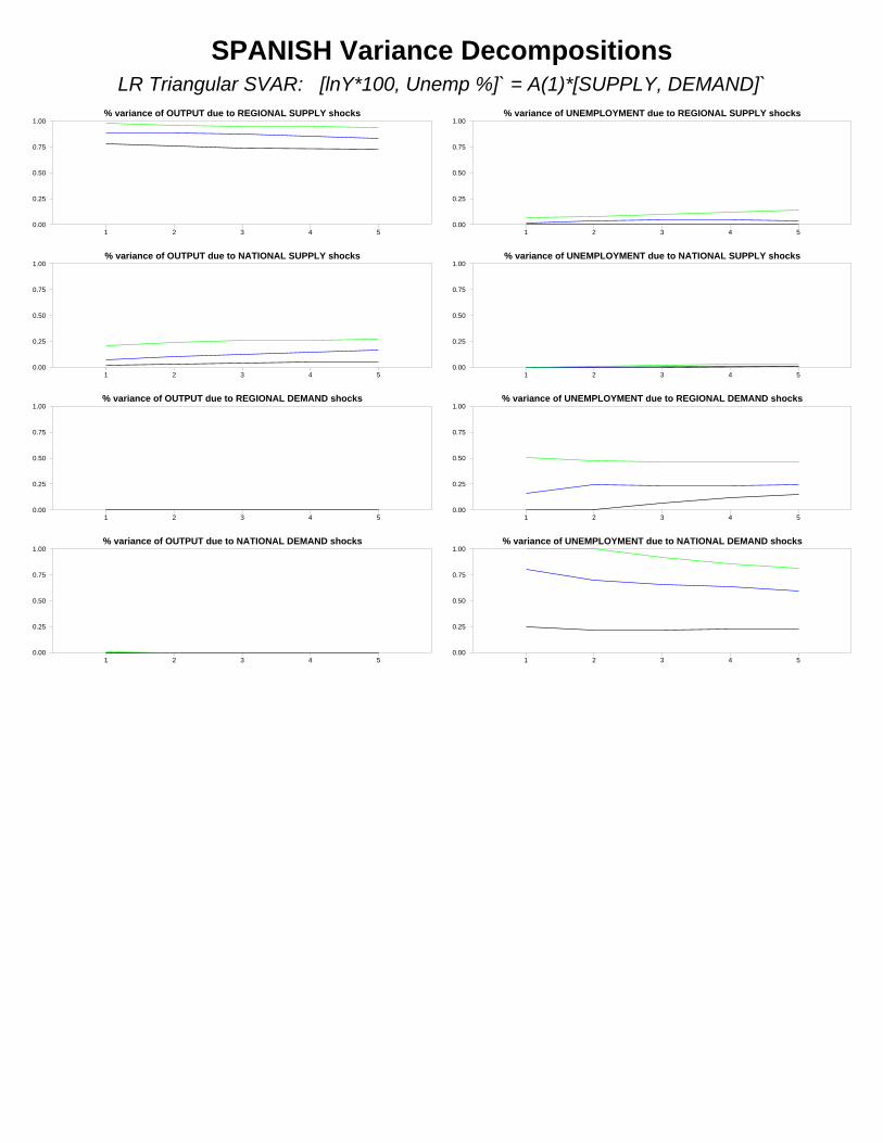
SPANISH Variance DecompositionsLR Triangular SVAR: [lnY*100, Unemp %]` = A(1)*[SUPPLY, DEMAND]`
% variance of OUTPUT due to REGIONAL SUPPLY shocks
1 2 3 4 50.00
0.25
0.50
0.75
1.00
% variance of OUTPUT due to NATIONAL SUPPLY shocks
1 2 3 4 50.00
0.25
0.50
0.75
1.00
% variance of OUTPUT due to REGIONAL DEMAND shocks
1 2 3 4 50.00
0.25
0.50
0.75
1.00
% variance of OUTPUT due to NATIONAL DEMAND shocks
1 2 3 4 50.00
0.25
0.50
0.75
1.00
% variance of UNEMPLOYMENT due to REGIONAL SUPPLY shocks
1 2 3 4 50.00
0.25
0.50
0.75
1.00
% variance of UNEMPLOYMENT due to NATIONAL SUPPLY shocks
1 2 3 4 50.00
0.25
0.50
0.75
1.00
% variance of UNEMPLOYMENT due to REGIONAL DEMAND shocks
1 2 3 4 50.00
0.25
0.50
0.75
1.00
% variance of UNEMPLOYMENT due to NATIONAL DEMAND shocks
1 2 3 4 50.00
0.25
0.50
0.75
1.00

SPANISH Impulse ResponsesLR Triangular SVAR: [lnY*100, Unemp %]` = A(1)*[SUPPLY, DEMAND]`response of OUTPUT to REGIONAL SUPPLY shocks
1 2 3 4 52.25
2.50
2.75
3.00
3.25
3.50
3.75
4.00
4.25
response of OUTPUT to NATIONAL SUPPLY shocks
1 2 3 4 50.75
1.00
1.25
1.50
1.75
2.00
response of OUTPUT to REGIONAL DEMAND shocks
1 2 3 4 5-0.3
-0.2
-0.1
0.0
0.1
0.2
0.3
response of OUTPUT to NATIONAL DEMAND shocks
1 2 3 4 5-0.15
-0.10
-0.05
0.00
0.05
0.10
0.15
response of UNEMPLOYMENT to REGIONAL SUPPLY shocks
1 2 3 4 5-0.8
-0.7
-0.6
-0.5
-0.4
-0.3
-0.2
-0.1
-0.0
0.1
response of UNEMPLOYMENT to NATIONAL SUPPLY shocks
1 2 3 4 5-0.40
-0.35
-0.30
-0.25
-0.20
-0.15
-0.10
-0.05
-0.00
0.05
response of UNEMPLOYMENT to REGIONAL DEMAND shocks
1 2 3 4 5-3.25
-3.00
-2.75
-2.50
-2.25
-2.00
-1.75
-1.50
-1.25
-1.00
response of UNEMPLOYMENT to NATIONAL DEMAND shocks
1 2 3 4 5-1.2
-1.1
-1.0
-0.9
-0.8
-0.7
-0.6
-0.5

ITALIAN Variance DecompositionsLR Triangular SVAR: [lnY*100, Unemp %]` = A(1)*[SUPPLY, DEMAND]`
% variance of OUTPUT due to REGIONAL SUPPLY shocks
1 2 3 4 50.00
0.25
0.50
0.75
1.00
% variance of OUTPUT due to NATIONAL SUPPLY shocks
1 2 3 4 50.00
0.25
0.50
0.75
1.00
% variance of OUTPUT due to REGIONAL DEMAND shocks
1 2 3 4 50.00
0.25
0.50
0.75
1.00
% variance of OUTPUT due to NATIONAL DEMAND shocks
1 2 3 4 50.00
0.25
0.50
0.75
1.00
% variance of UNEMPLOYMENT due to REGIONAL SUPPLY shocks
1 2 3 4 50.00
0.25
0.50
0.75
1.00
% variance of UNEMPLOYMENT due to NATIONAL SUPPLY shocks
1 2 3 4 50.00
0.25
0.50
0.75
1.00
% variance of UNEMPLOYMENT due to REGIONAL DEMAND shocks
1 2 3 4 50.00
0.25
0.50
0.75
1.00
% variance of UNEMPLOYMENT due to NATIONAL DEMAND shocks
1 2 3 4 50.00
0.25
0.50
0.75
1.00

ITALIAN Impulse ResponsesLR Triangular SVAR: [lnY*100, Unemp %]` = A(1)*[SUPPLY, DEMAND]`response of OUTPUT to REGIONAL SUPPLY shocks
1 2 3 4 51.25
1.50
1.75
2.00
2.25
2.50
2.75
3.00
3.25
response of OUTPUT to NATIONAL SUPPLY shocks
1 2 3 4 50.50
0.75
1.00
1.25
1.50
response of OUTPUT to REGIONAL DEMAND shocks
1 2 3 4 5-0.2
-0.1
0.0
0.1
0.2
0.3
0.4
0.5
0.6
0.7
response of OUTPUT to NATIONAL DEMAND shocks
1 2 3 4 5-0.10
-0.05
0.00
0.05
0.10
0.15
0.20
0.25
0.30
response of UNEMPLOYMENT to REGIONAL SUPPLY shocks
1 2 3 4 5-0.10
-0.05
0.00
0.05
0.10
0.15
0.20
0.25
0.30
0.35
response of UNEMPLOYMENT to NATIONAL SUPPLY shocks
1 2 3 4 5-0.04
-0.02
0.00
0.02
0.04
0.06
0.08
0.10
0.12
response of UNEMPLOYMENT to REGIONAL DEMAND shocks
1 2 3 4 5-1.4
-1.2
-1.0
-0.8
-0.6
-0.4
-0.2
response of UNEMPLOYMENT to NATIONAL DEMAND shocks
1 2 3 4 5-0.7
-0.6
-0.5
-0.4
-0.3
-0.2
-0.1

FRENCH Variance DecompositionsLR Triangular SVAR: [lnY*100, Unemp %]` = A(1)*[SUPPLY, DEMAND]`
% variance of OUTPUT due to REGIONAL SUPPLY shocks
1 2 3 4 50.00
0.25
0.50
0.75
1.00
% variance of OUTPUT due to NATIONAL SUPPLY shocks
1 2 3 4 50.00
0.25
0.50
0.75
1.00
% variance of OUTPUT due to REGIONAL DEMAND shocks
1 2 3 4 50.00
0.25
0.50
0.75
1.00
% variance of OUTPUT due to NATIONAL DEMAND shocks
1 2 3 4 50.00
0.25
0.50
0.75
1.00
% variance of UNEMPLOYMENT due to REGIONAL SUPPLY shocks
1 2 3 4 50.00
0.25
0.50
0.75
1.00
% variance of UNEMPLOYMENT due to NATIONAL SUPPLY shocks
1 2 3 4 50.00
0.25
0.50
0.75
1.00
% variance of UNEMPLOYMENT due to REGIONAL DEMAND shocks
1 2 3 4 50.00
0.25
0.50
0.75
1.00
% variance of UNEMPLOYMENT due to NATIONAL DEMAND shocks
1 2 3 4 50.00
0.25
0.50
0.75
1.00

FRENCH Impulse ResponsesLR Triangular SVAR: [lnY*100, Unemp %]` = A(1)*[SUPPLY, DEMAND]`response of OUTPUT to REGIONAL SUPPLY shocks
1 2 3 4 51.8
2.0
2.2
2.4
2.6
2.8
3.0
response of OUTPUT to NATIONAL SUPPLY shocks
1 2 3 4 50.8
0.9
1.0
1.1
1.2
1.3
1.4
1.5
response of OUTPUT to REGIONAL DEMAND shocks
1 2 3 4 5-0.1
0.0
0.1
0.2
0.3
0.4
0.5
response of OUTPUT to NATIONAL DEMAND shocks
1 2 3 4 5-0.05
0.00
0.05
0.10
0.15
0.20
0.25
response of UNEMPLOYMENT to REGIONAL SUPPLY shocks
1 2 3 4 5-0.4
-0.3
-0.2
-0.1
-0.0
0.1
0.2
response of UNEMPLOYMENT to NATIONAL SUPPLY shocks
1 2 3 4 5-0.20
-0.15
-0.10
-0.05
-0.00
0.05
0.10
response of UNEMPLOYMENT to REGIONAL DEMAND shocks
1 2 3 4 5-1.1
-1.0
-0.9
-0.8
-0.7
-0.6
-0.5
response of UNEMPLOYMENT to NATIONAL DEMAND shocks
1 2 3 4 5-0.55
-0.50
-0.45
-0.40
-0.35
-0.30
-0.25
-0.20

SPANISH Individual Country Impulse ResponsesLR Triangular SVAR: [lnY*100, Unemp %]` = A(1)*[SUPPLY, DEMAND]`response of OUTPUT to REGIONAL SUPPLY shocks
1 2 3 4 51
2
3
4
5
6
7
response of OUTPUT to NATIONAL SUPPLY shocks
1 2 3 4 50.5
1.0
1.5
2.0
2.5
3.0
3.5
response of OUTPUT to REGIONAL DEMAND shocks
1 2 3 4 5-1.5
-1.0
-0.5
0.0
0.5
1.0
1.5
response of OUTPUT to NATIONAL DEMAND shocks
1 2 3 4 5-0.6
-0.4
-0.2
0.0
0.2
0.4
0.6
response of UNEMPLOYMENT to REGIONAL SUPPLY shocks
1 2 3 4 5-2.5
-2.0
-1.5
-1.0
-0.5
0.0
0.5
response of UNEMPLOYMENT to NATIONAL SUPPLY shocks
1 2 3 4 5-1.2
-1.0
-0.8
-0.6
-0.4
-0.2
-0.0
0.2
response of UNEMPLOYMENT to REGIONAL DEMAND shocks
1 2 3 4 5-9
-8
-7
-6
-5
-4
-3
-2
-1
0
response of UNEMPLOYMENT to NATIONAL DEMAND shocks
1 2 3 4 5-3.5
-3.0
-2.5
-2.0
-1.5
-1.0
-0.5
0.0

SPANISH Regional OUTPUT responseto NATIONAL SUPPLY shocks
Regional population (000s)
lnY*
100
by y
ear 2
0 2000 4000 6000 80000.6
0.8
1.0
1.2
1.4
1.6
1.8
2.0
2.2
2.4
Galicia
Asturias
Cantabria
Pais VascoNavarra
Rioja
Aragón
Madrid
Castilla y León
Castilla-la Mancha
ExtremaduraCataluña
Valenciana
Illes Balears
Andalucia
Murcia
CeutaMelilla
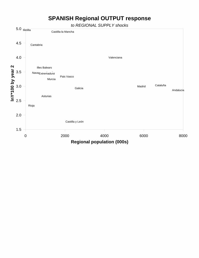
SPANISH Regional OUTPUT responseto REGIONAL SUPPLY shocks
Regional population (000s)
lnY*
100
by y
ear 2
0 2000 4000 6000 80001.5
2.0
2.5
3.0
3.5
4.0
4.5
5.0
Galicia
Asturias
Cantabria
Pais VascoNavarra
Rioja
Aragón
Madrid
Castilla y León
Castilla-la Mancha
Extremadura
Cataluña
Valenciana
Illes Balears
Andalucia
Murcia
CeutaMelilla

SPANISH Regional OUTPUT responseto NATIONAL DEMAND shocks
Regional population (000s)
lnY*
100
by y
ear 2
0 2000 4000 6000 8000-0.5
-0.4
-0.3
-0.2
-0.1
-0.0
0.1
0.2
0.3
GaliciaAsturias
Cantabria
Pais Vasco
NavarraRioja
Aragón
Madrid
Castilla y León
Castilla-la Mancha
Extremadura
CataluñaValenciana
Illes Balears
Andalucia
Murcia
Ceuta
Melilla

SPANISH Regional UNEMPLOYMENT responseto NATIONAL SUPPLY shocks
Regional population (000s)
Une
mp
% b
y ye
ar 2
0 2000 4000 6000 8000-0.8
-0.7
-0.6
-0.5
-0.4
-0.3
-0.2
-0.1
-0.0
0.1
Galicia
Asturias
Cantabria
Pais VascoNavarra
Rioja
Aragón
MadridCastilla y León
Castilla-la ManchaExtremadura
Cataluña
ValencianaIlles Balears
Andalucia
MurciaCeuta
Melilla
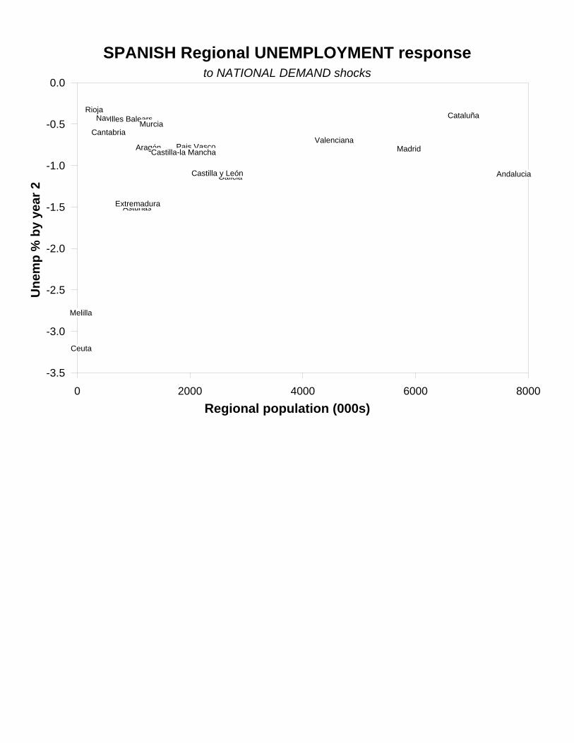
SPANISH Regional UNEMPLOYMENT responseto NATIONAL DEMAND shocks
Regional population (000s)
Une
mp
% b
y ye
ar 2
0 2000 4000 6000 8000-3.5
-3.0
-2.5
-2.0
-1.5
-1.0
-0.5
0.0
Galicia
Asturias
Cantabria
Pais Vasco
NavarraRioja
Aragón Madrid
Castilla y León
Castilla-la Mancha
Extremadura
Cataluña
Valenciana
Illes Balears
Andalucia
Murcia
Ceuta
Melilla

SPANISH Regional OUTPUT responseto NATIONAL SUPPLY shocks
Financial intermediation location quotient
lnY*
100
by y
ear 2
25 50 75 100 125 1500.6
0.8
1.0
1.2
1.4
1.6
1.8
2.0
2.2
2.4
Galicia
Asturias
Cantabria
Pais VascoNavarra
Rioja
Aragón
Madrid
Castilla y León
Castilla-la Mancha
ExtremaduraCataluña
Valenciana
Illes Balears
Andalucia
Murcia
CeutaMelilla

SPANISH Regional OUTPUT responseto NATIONAL DEMAND shocks
Financial intermediation location quotient
lnY*
100
by y
ear 2
25 50 75 100 125 150-0.5
-0.4
-0.3
-0.2
-0.1
-0.0
0.1
0.2
0.3
GaliciaAsturias
Cantabria
Pais Vasco
NavarraRioja
Aragón
Madrid
Castilla y León
Castilla-la Mancha
Extremadura
CataluñaValenciana
Illes Balears
Andalucia
Murcia
Ceuta
Melilla

SPANISH Regional OUTPUT responseto REGIONAL DEMAND shocks
Financial intermediation location quotient
lnY*
100
by y
ear 2
25 50 75 100 125 150-1.00
-0.75
-0.50
-0.25
0.00
0.25
0.50
GaliciaAsturias
Cantabria
Pais Vasco
NavarraRioja
Aragón
Madrid
Castilla y León
Castilla-la Mancha
Extremadura
Cataluña
Valenciana
Illes Balears
Andalucia
Murcia
Ceuta
Melilla

ITALIAN Regional OUTPUT responseto NATIONAL SUPPLY shocks
Regional population (000s)
lnY*
100
by y
ear 2
0 2000 4000 6000 8000 100000.00
0.25
0.50
0.75
1.00
1.25
1.50
1.75
2.00
Piemonte
Aosta
LiguriaLombardia
Bolzano-Bozen
Trento
Veneto
Friuli-VGiulia
Emilia-Romagna
ToscanaUmbria
Marche
Lazio
Abruzzo
Molise
Campania
Puglia
Basilicata
Calabria
Sicilia
Sardegna
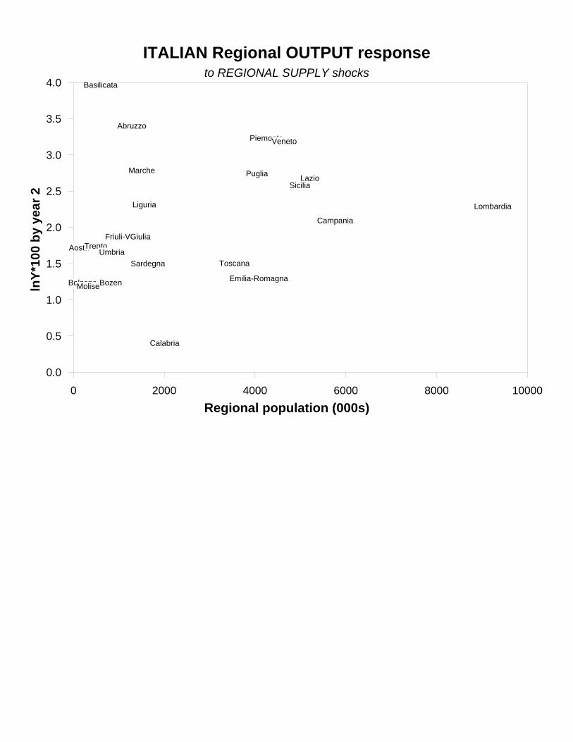
ITALIAN Regional OUTPUT responseto REGIONAL SUPPLY shocks
Regional population (000s)
lnY*
100
by y
ear 2
0 2000 4000 6000 8000 100000.0
0.5
1.0
1.5
2.0
2.5
3.0
3.5
4.0
Piemonte
Aosta
Liguria Lombardia
Bolzano-Bozen
Trento
Veneto
Friuli-VGiulia
Emilia-Romagna
ToscanaUmbria
MarcheLazio
Abruzzo
Molise
Campania
Puglia
Basilicata
Calabria
Sicilia
Sardegna

ITALIAN Regional UNEMPLOYMENT responseto NATIONAL DEMAND shocks
Regional population (000s)
Une
mp
% b
y ye
ar 2
0 2000 4000 6000 8000 10000-1.00
-0.75
-0.50
-0.25
0.00
Piemonte
Aosta
Liguria
Lombardia
Bolzano-Bozen
Trento
Veneto
Friuli-VGiulia
Emilia-Romagna
Toscana
Umbria
Marche
Lazio
AbruzzoMolise
Campania
Puglia
Basilicata
Calabria
Sicilia
Sardegna

ITALIAN Regional UNEMPLOYMENT responseto NATIONAL DEMAND shocks
Financial intermediation location quotient
Une
mp
% b
y ye
ar 2
60 80 100 120 140-1.00
-0.75
-0.50
-0.25
0.00
Piemonte
Aosta
Liguria
Lombardia
Bolzano-Bozen
Trento
Veneto
Friuli-VGiulia
Emilia-Romagna
Toscana
Umbria
Marche
Lazio
AbruzzoMolise
Campania
Puglia
Basilicata
Calabria
Sicilia
Sardegna

ITALIAN Regional OUTPUT responseto REGIONAL SUPPLY shocks
Chemicals and petro refining location quotient
lnY*
100
by y
ear 2
0 50 100 150 200 2500.0
0.5
1.0
1.5
2.0
2.5
3.0
3.5
4.0
Piemonte
Aosta
Liguria Lombardia
Bolzano-Bozen
Trento
Veneto
Friuli-VGiulia
Emilia-Romagna
ToscanaUmbria
MarcheLazio
Abruzzo
Molise
Campania
Puglia
Basilicata
Calabria
Sicilia
Sardegna

ITALIAN Regional OUTPUT responseto NATIONAL SUPPLY shocks
Chemicals and petro refining location quotient
lnY*
100
by y
ear 2
0 50 100 150 200 2500.00
0.25
0.50
0.75
1.00
1.25
1.50
1.75
2.00
Piemonte
Aosta
LiguriaLombardia
Bolzano-Bozen
Trento
Veneto
Friuli-VGiulia
Emilia-Romagna
ToscanaUmbria
Marche
Lazio
Abruzzo
Molise
Campania
Puglia
Basilicata
Calabria
Sicilia
Sardegna

ITALIAN Regional OUTPUT responseto NATIONAL DEMAND shocks
Chemicals and petro refining location quotient
lnY*
100
by y
ear 2
0 50 100 150 200 250-0.25
0.00
0.25
0.50
0.75
1.00
Piemonte
Aosta
Liguria
Lombardia
Bolzano-BozenTrento
Veneto
Friuli-VGiulia
Emilia-Romagna
ToscanaUmbria
Marche
Lazio
Abruzzo
Molise
CampaniaPuglia
Basilicata
Calabria
SiciliaSardegna

ITALIAN Regional OUTPUT responseto REGIONAL DEMAND shocks
Chemicals and petro refining location quotient
lnY*
100
by y
ear 2
0 50 100 150 200 250-0.5
0.0
0.5
1.0
1.5
2.0
Piemonte
Aosta Liguria
Lombardia
Bolzano-BozenTrento
Veneto
Friuli-VGiulia
Emilia-Romagna
Toscana
Umbria
Marche
Lazio
Abruzzo
Molise
CampaniaPuglia
Basilicata
Calabria
SiciliaSardegna

ITALIAN Regional UNEMPLOYMENT responseto NATIONAL DEMAND shocks
Chemicals and petro refining location quotient
Une
mp
% b
y ye
ar 2
0 50 100 150 200 250-1.00
-0.75
-0.50
-0.25
0.00
Piemonte
Aosta
Liguria
Lombardia
Bolzano-Bozen
Trento
Veneto
Friuli-VGiulia
Emilia-Romagna
Toscana
Umbria
Marche
Lazio
AbruzzoMolise
Campania
Puglia
Basilicata
Calabria
Sicilia
Sardegna

ITALIAN Regional UNEMPLOYMENT responseto REGIONAL SUPPLY shocks
Chemicals and petro refining location quotient
Une
mp
% b
y ye
ar 2
0 50 100 150 200 250-0.6
-0.4
-0.2
0.0
0.2
0.4
0.6
0.8
1.0
1.2
Piemonte
Aosta
Liguria
Lombardia
Bolzano-Bozen
Trento Veneto
Friuli-VGiulia
Emilia-Romagna
Toscana
Umbria
Marche
Lazio
Abruzzo
Molise
Campania
Puglia
Basilicata
Calabria
Sicilia
Sardegna

ITALIAN Regional OUTPUT responseto REGIONAL DEMAND shocks
Agriculture location quotient
lnY*
100
by y
ear 2
0 50 100 150 200 250 300 350-0.5
0.0
0.5
1.0
1.5
2.0
Piemonte
AostaLiguria
Lombardia
Bolzano-BozenTrento
Veneto
Friuli-VGiulia
Emilia-Romagna
Toscana
Umbria
Marche
Lazio
Abruzzo
Molise
CampaniaPuglia
Basilicata
Calabria
SiciliaSardegna

ITALIAN Regional UNEMPLOYMENT responseto NATIONAL DEMAND shocks
Agriculture location quotient
Une
mp
% b
y ye
ar 2
0 50 100 150 200 250 300 350-1.00
-0.75
-0.50
-0.25
0.00
Piemonte
Aosta
Liguria
Lombardia
Bolzano-Bozen
Trento
Veneto
Friuli-VGiulia
Emilia-Romagna
Toscana
Umbria
Marche
Lazio
AbruzzoMolise
Campania
Puglia
Basilicata
Calabria
Sicilia
Sardegna
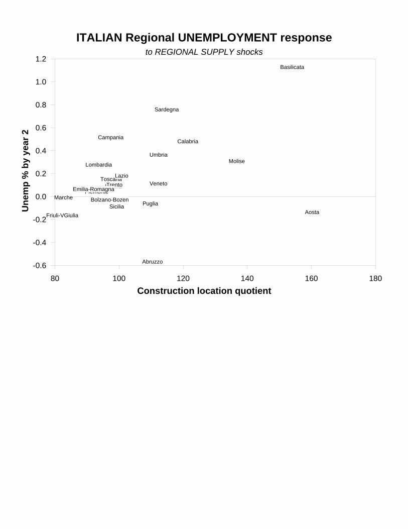
ITALIAN Regional UNEMPLOYMENT responseto REGIONAL SUPPLY shocks
Construction location quotient
Une
mp
% b
y ye
ar 2
80 100 120 140 160 180-0.6
-0.4
-0.2
0.0
0.2
0.4
0.6
0.8
1.0
1.2
Piemonte
Aosta
Liguria
Lombardia
Bolzano-Bozen
Trento Veneto
Friuli-VGiulia
Emilia-Romagna
Toscana
Umbria
Marche
Lazio
Abruzzo
Molise
Campania
Puglia
Basilicata
Calabria
Sicilia
Sardegna

ITALIAN Regional UNEMPLOYMENT responseto NATIONAL DEMAND shocks
Construction location quotient
Une
mp
% b
y ye
ar 2
80 100 120 140 160 180-1.00
-0.75
-0.50
-0.25
0.00
Piemonte
Aosta
Liguria
Lombardia
Bolzano-Bozen
Trento
Veneto
Friuli-VGiulia
Emilia-Romagna
Toscana
Umbria
Marche
Lazio
AbruzzoMolise
Campania
Puglia
Basilicata
Calabria
Sicilia
Sardegna

ITALIAN Regional OUTPUT responseto REGIONAL DEMAND shocks
Mining quarrying and energy supply location quotient
lnY*
100
by y
ear 2
0 50 100 150 200 250 300 350-0.5
0.0
0.5
1.0
1.5
2.0
Piemonte
AostaLiguria
Lombardia
Bolzano-BozenTrento
Veneto
Friuli-VGiulia
Emilia-Romagna
Toscana
Umbria
Marche
Lazio
Abruzzo
Molise
CampaniaPuglia
Basilicata
Calabria
SiciliaSardegna
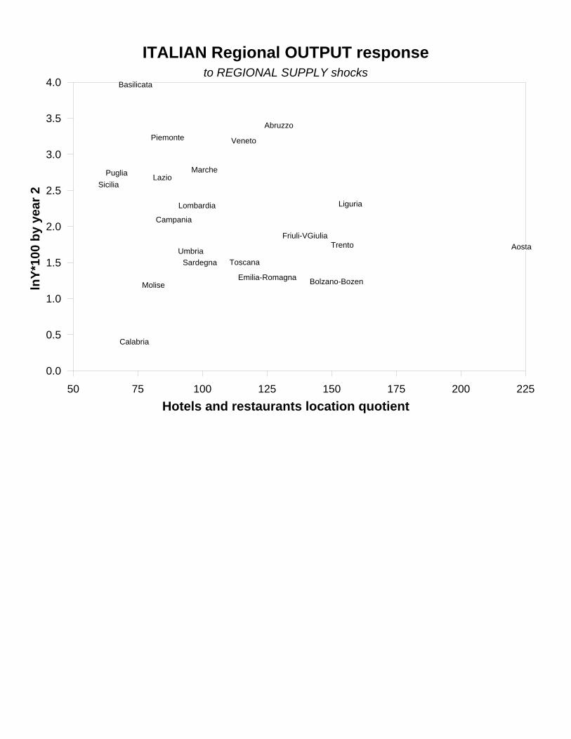
ITALIAN Regional OUTPUT responseto REGIONAL SUPPLY shocks
Hotels and restaurants location quotient
lnY*
100
by y
ear 2
50 75 100 125 150 175 200 2250.0
0.5
1.0
1.5
2.0
2.5
3.0
3.5
4.0
Piemonte
Aosta
LiguriaLombardia
Bolzano-Bozen
Trento
Veneto
Friuli-VGiulia
Emilia-Romagna
ToscanaUmbria
MarcheLazio
Abruzzo
Molise
Campania
Puglia
Basilicata
Calabria
Sicilia
Sardegna
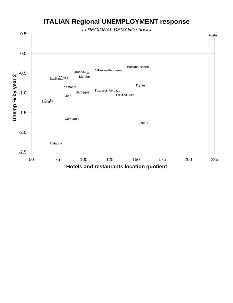
ITALIAN Regional UNEMPLOYMENT responseto REGIONAL DEMAND shocks
Hotels and restaurants location quotient
Une
mp
% b
y ye
ar 2
50 75 100 125 150 175 200 225-2.5
-2.0
-1.5
-1.0
-0.5
0.0
0.5
Piemonte
Aosta
Liguria
Lombardia
Bolzano-Bozen
Trento
Veneto
Friuli-VGiulia
Emilia-Romagna
Toscana
UmbriaMarche
LazioAbruzzo
Molise
Campania
Puglia
Basilicata
Calabria
Sicilia
Sardegna

FRENCH Regional OUTPUT responseto NATIONAL SUPPLY shocks
Regional population (000s)
lnY*
100
by y
ear 2
0 2000 4000 6000 8000 10000 120000.0
0.5
1.0
1.5
2.0
2.5
3.0
Île de France
Champagne-Ardenne
Picardie
Haute-Normandie
Centre
Basse-Normandie
BourgogneCalais
Lorraine
Alsace
Franche-Comté
Loire
Bretagne
Poitou-Charentes
Aquitaine
Pyrénées
Limousin
Rhône
Auvergne
Languedoc-Roussillon
Provence
Corse

FRENCH Regional UNEMPLOYMENT responseto NATIONAL DEMAND shocks
Regional population (000s)
Une
mp
% b
y ye
ar 2
0 2000 4000 6000 8000 10000 12000-2.00
-1.75
-1.50
-1.25
-1.00
-0.75
-0.50
-0.25
0.00
Île de France
Champagne-ArdennePicardie
Haute-Normandie
CentreBasse-NormandieBourgogne
Calais
Lorraine
Alsace
Franche-ComtéLoire
Bretagne
Poitou-CharentesAquitaine PyrénéesLimousin
Rhône
Auvergne
Languedoc-Roussillon
Provence
Corse

FRENCH Regional OUTPUT responseto NATIONAL SUPPLY shocks
Construction location quotient
lnY*
100
by y
ear 2
70 80 90 100 110 1200.0
0.5
1.0
1.5
2.0
2.5
3.0
Île de France
Champagne-Ardenne
Picardie
Haute-Normandie
Centre
Basse-Normandie
BourgogneCalais
Lorraine
Alsace
Franche-Comté
Loire
Bretagne
Poitou-Charentes
Aquitaine
Pyrénées
Limousin
Rhône
Auvergne
Languedoc-Roussillon
Provence
Corse

FRENCH Regional OUTPUT responseto REGIONAL DEMAND shocks
Mining quarrying and energy supply location quotient
lnY*
100
by y
ear 2
60 80 100 120 140 160-0.1
0.0
0.1
0.2
0.3
0.4
0.5
0.6
Île de France
Champagne-Ardenne
Picardie
Haute-Normandie
Centre
Basse-Normandie
Bourgogne
Calais
Lorraine
Alsace
Franche-Comté
Loire
Bretagne
Poitou-Charentes
Aquitaine Pyrénées
Limousin
Rhône
Auvergne
Languedoc-Roussillon
Provence
Corse

FRENCH Regional OUTPUT responseto NATIONAL DEMAND shocks
Mining quarrying and energy supply location quotient
lnY*
100
by y
ear 2
60 80 100 120 140 160-0.05
0.00
0.05
0.10
0.15
0.20
0.25
0.30
Île de France
Champagne-Ardenne
Picardie
Haute-Normandie
Centre
Basse-Normandie
Bourgogne
Calais
Lorraine
Alsace
Franche-Comté
Loire
Bretagne
Poitou-Charentes
Aquitaine Pyrénées
Limousin
Rhône
Auvergne
Languedoc-Roussillon
Provence
Corse
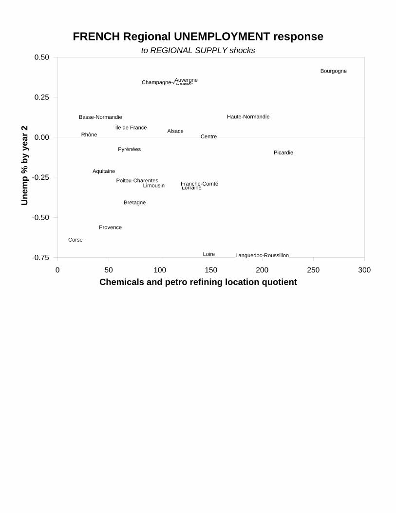
FRENCH Regional UNEMPLOYMENT responseto REGIONAL SUPPLY shocks
Chemicals and petro refining location quotient
Une
mp
% b
y ye
ar 2
0 50 100 150 200 250 300-0.75
-0.50
-0.25
0.00
0.25
0.50
Île de France
Champagne-Ardenne
Picardie
Haute-Normandie
Centre
Basse-Normandie
Bourgogne
Calais
Lorraine
Alsace
Franche-Comté
Loire
Bretagne
Poitou-Charentes
Aquitaine
Pyrénées
Limousin
Rhône
Auvergne
Languedoc-Roussillon
Provence
Corse

FRENCH Regional UNEMPLOYMENT responseto NATIONAL SUPPLY shocks
Mining quarrying and energy supply location quotient
Une
mp
% b
y ye
ar 2
60 80 100 120 140 160-0.4
-0.3
-0.2
-0.1
-0.0
0.1
0.2
0.3
Île de France
Champagne-Ardenne
Picardie
Haute-Normandie
Centre
Basse-Normandie
Bourgogne
Calais
Lorraine
Alsace
Franche-Comté
Loire
Bretagne
Poitou-Charentes
Aquitaine
Pyrénées
Limousin
Rhône
Auvergne
Languedoc-Roussillon ProvenceCorse

429
Other Examples of Panel SVAR Applications: (Work in Progress)
“The Contribution of Housing Markets to the Great Recession” Pedroni & Sheppard (2010)
- uses Moody’s regional U.S. metropolitan level data
- studies role of local U.S. housing markets in contributing to current U.S. and Global recession
“Monetary Policy in Low Income Countries” Mishra, Montiel, Pedroni & Spilimbergo (2010)
- uses country level IFS data
- studies differences in effectiveness and transmission mechanisms of monetary policy among countries