presented in partial fulfillment of the requirement for
TRANSCRIPT
The Analysis of Factors That Affect The Demand of Red Chili in Blimbing
District of Malang
JOURNAL
Presented in Partial Fulfillment of the requirement for the Degree of
Bachelor in Economics
BY:
PUTRI LAHARWATI
NIM. 105020103121001
INTERNATIONAL UNDERGRADUATE PROGRAM IN ECONOMICS
FACULTY OF ECONOMIC AND BUSINESS
UNIVERSITAS BRAWIJAYA
MALANG
2014

THE ANALYSIS OF FACTORS THAT AFFECT THE DEMAND OF
RED CHILI IN BLIMBING DISTRICT OF MALANG
Laharwati, Putri. 2014. The Analysis of Factors That Affect The Demand of Red Chili in
Blimbing District of Malang. Minor Thesis. International Undergraduate Program in
Economics, Faculty of Economic and Business, Brawijaya University. With supervisor
Dr. Khusnul Ashar, SE.,MA.
Abstract
The aim of this research are to To analyze the factors that influence the demand of red
chili partially and simultaneously and to analyze the elasticities demand of red chili.
The approach of reasearch used quantitative, with research method using multiple
linier regression. While the data used are primary and secondary which taken from direct
survey, related institutions, and official government website.
The result shows that partially the variables of price of red chili, price of substitution
good, price of complementary good, and the number of population are not significant to the
demand of red chili in Blimbing District, while the variables of spicy culinary restaurant’s
income and number of spicy culinary restaurant are significant to the demand of red chili in
Blimbing District. Moreover, simultaneously the variables of price of red chili, price of
substitution good, price of complementary good, the number of population, spicy culinary
restaurant’s income, and number of spicy culinary restaurant are significant to the demand of
red chili in Blimbing District. Whereas the variables of spicy culinary restaurant’s income
have the income elasticity value as amount 0.182 and the income elasticity for the number of
spicy culinary restaurant as amount 0.323.
1.Background
One of horticultural commodities is red chili. Red chili (Capsicum annuum L) is one
kind of commercial vegetables that have long been cultivated in Indonesia, because the
product has a high economic value. Moreover to fullfil the needs of everyday households,
chili is widely used as raw material for food and pharmaceutical industries. Although chili is
not main food for Indonesian people, but the commodities cannot be abandoned. Chili, not
only can be eaten freshly as a mixture seasoning, but also preserved in the form of chili
sauces, pasta pickles, dried fruit and flour (Dewi, 2009).
Demand for chili being expected will continue to increase along with the increase in
income and population. The increase in income and population is directly improves the
people's need, so the demand of chili fluctuates in the retail market. Various supply and
demand factors also cause fluctuations in the price of chili, so the equilibrium price that
occurs in the condition of the amount offered is relatively much less than the amount
requested. This is resulting in price which is being very high.
The rise of spicy food seller in Malang is one of high potential bussines fields which
are very common nowadays. The number of consumer enjoying spicy foods stimulate the
growth of spicy cuisine business, ranging from spicy noodles, spicy chicken, until spicy
chicken claw. Those are caused by the location of Malang that is located in a highland
surrounded by mountain and tends to have cold temperature, triggering spicy taste on almost
every kind of food consumption. So that spicy taste which originated from chili is main
commodity and seasoning for most people especially in Malang.
2.Problem Identification
From the explanation above, the problems that need to be disscused related to
demand of chili in Blimbing District are:
1. What factors that cause the demand of red chili partially and simultaneously?

2. How the elasticities demand of red chili?
3.Research Purposes
1. To analyze the factors that influence the demand of red chili partially and
simultaneously.
2. To analyze the elasticities demand of red chili .
4.Theoritical Framework
Theory of Demand
In the law of demand explained the nature of the relationship between the demand of
goods and the price level. The law of demand is essentially a hypothesis: the lower price of
an item, the more demand for these goods. Conversely, the higher price of an item, the less
demand for such goods. The nature of this relationship, first due to the price increase causes
the buyer looks for the other items that can be used as a substitute for the goods that the price
has been increased. Conversely, if the price decrease then people will reduce purchases of
other goods of the same type and adding the purchase towards the goods that the price has
been decreased. Second, the increase in price causes buyers reduced real income. Revenue
slump forced the buyers to decrease purchasing various types of goods, and particularly for
the goods that the price has been increased (Sukirno, 2003).
Price Determination Theory
According to Tjiptono Fandy (2008) method of determination broadly grouped into
four main categories method, that are demand pricing-based, costs-based, profit-based, and
competition-based.
a. Demand Pricing-Based Method
This method emphasizes the factors that influence the tastes and preferences of
customers rather than other factors such as cost, profit, and competition. Customer
demand itself based on various consideration, such as: The ability of customers to buy
(purchase power parity); The willingness of customers to buy; The position of product
in customers lifestyle, that related to whether the product as a status symbol or just a
product; The benefits that given from the products to the customers; The prices of
substitution products
b. Costs-Based Method
In this method the major determinant is the aspect of supply or cost, not the aspect
of demand. Price is determined based on the cost of production and marketing coupled
with a certain amount so as to cover the direct costs, overhead costs, and profit.
c. Profit-Based Method
This method tries to balance revenue and costs in its pricing. This work is done on
the basis of target specific profit volume or expressed as a percentage toward sales and
investment.
d. Competition-Based Methods
In addition based on considerations of cost, demand, or income price can also be
determined on the basis of competition, which is what the competitor is doing.
Competition-based pricing method consists of four kinds: the customary pricing, above,
at, or below market pricing, loss leader pricing, bid pricing sealer.
Demand Elasticity Concept
Measurement that can be used to determine the relationship between the demand with the
factors that influence is demand elasticity. The elasticity of demand can be divided into three
(3) types, they are: Price elasticity; Income elasticity; Cross elasticity (Burhan, 2006)
a. Price Elasticity
The widest size of the elasticity used is price elasticity of demand, which
measures the responsive of quantity demanded toward changes in price of the product,

by maintaining the value of all other variables in constant demand function. By using
the point elasticity formula, the price elasticity of demand found as follows:
ɛ
(Pappas dan Mark H, 1995).
b. Income Elasticity
Income elasticity of demand measures the responsiveness of demand to
changes in income, by maintaining the influence of all other variables remain
constant. If (I) represent income, the income elasticity point is defined as follows:
ɛI
Income and the amount of purchased is generally moving to the same direction, i.e
revenue and sales directly related and not in reverse (Pappas and Mark H, 1995).
c. Cross Elasticity
The concept of cross-price elasticity is used to examine the responsiveness of
demand for one product for changes in the price of other products. Cross-price
elasticity of demand is known by the following:
ɛpx
where Y and X are two different products. Cross-price elasticity for substitutes is
always positive, the price of the goods and the demand for other goods always moving
to the same direction. Cross-price elasticity is negative for complementary, price and
number moves to reverse direction. The last, cross-price elasticity of zero, or close to
zero, for the goods that are not related, variations in the price of one good do not
affect the demand for both goods (Pappas and Mark H , 1995).
5. Hypothesis
1. It is expected that the price itself (red chili price), price of big red chili, price of
onion, number of population, spicy culinary restaurant’s income, and the number of
spicy culinary food restaurant partially influenced toward the demand of chili in
Blimbing District of Malang. It is expected that the price itself (red chili price), price
of big red chili, price of onion, number of population, spicy culinary restaurant’s
income, and the number of spicy culinary food restaurant simultaneously influenced
toward the demand of chilli in Blimbing District of Malang.
2. It is expected that income has positive elasticity toward the demand of red chili.
6.Research Methodology
Research Design
According to Robert Donmoyer (Given, 2008) quantitative research method is the
approaching against to empirical studies to collect, analyze, and shows the data that in the
form of numerical rather than narrative.
The reason why researcher using quantitative method because the objective of
quantitative method is to develop and lies mathematical models, theories, and hypothesis
related to phenomena. Correlation between those variables either to test whether the result
has positive or negative correlation between each others. So that the researcher can avoiding
bias of the focus of research (elaboration, explanation, and forecast).
Definition of Variables
Definition of operational is a definition that is given to variable or construct by way
of giving a meaning, or specifies the activities, or provide an operational necessary to
construct or set these variables (Nazir, 2003). Operational definitions that used in this
research are the following :
a. Dependent Variables
Demand (Y) here are obtained from how dependent variables have the effect on
independent variables.
b. Independent Variables
1. Price of Red Chili (X1)
In previous research, price of red chili itself is the main factor that influenced
demand.
2. Price of Big Red Chili as Substitution Good (X2)
The good is called substitution toward other good if those were used as
replacement.
Big red chili used as substitution good because they have the same benefit and
usage. The spicy flavor of big red chili used as replacement of spicy flavor of red
chili. This substitution good have identical spicy taste of red chili even though they
are not 100% similar in term of hot flavor level.
3. Price of Onion as Complementary Good (X3)
The good is called complementary toward another good if they were used
together.
Onion can be called as complementary goods of red chili because they were
used together as complement.
4. Number of Population (X4)
The number of population which took in Blimbing District hold the main role
facing the high demand toward chili. The higher the number of population, the
higher the demand of red chili.
The number of population used as sample is the number of Blimbing District
population since 2011-2014.
5. Spicy Culinary Restaurant’s Income (X5)
Spicy culinary restaurant’s income is the measurement indicator of society
purchase power parity in consuming spicy food. The higher spicy cullinary
restaurant’s income, the higher purchase power parity of society toward spicy food
of red chili.
The income of these restaurants taken as sample is the amount of spicy
culinary restaurants which are located in Blimbing District since early 2011-2014
and has accountancy of gross income.
6. Number of Spicy Culinary Restaurant (X6)
The more spicy food business grows directly have the influence toward higher
demand of chili. It is required at least 5-10 kg of red chili for each spicy culinary
restaurant in Blimbing District, such as spicy noodle restaurant and spicy chicken
claw small stalls.
7.Results of Classical Assumptions Test
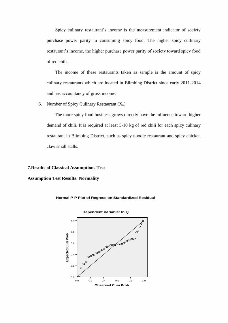
Assumption Test Results: Normality
1.00.80.60.40.20.0
Observed Cum Prob
1.0
0.8
0.6
0.4
0.2
0.0
Exp
ecte
d C
um
Pro
b
Normal P-P Plot of Regression Standardized Residual
Dependent Variable: ln.Q

Source: SPSS Data processed, 2014.
Figure 7.1 Normality Assumption Test Result
The result of the analysis in Figure 4.8 shows that the line describes the data actually
follows the diagonal line, so it can be concluded that the regression model obtained has a
normal distribution.
Assumption Test Results: Multicollinearity
Multicollinearity occurs when the VIF value is greater than 10. Good regression model
does not have multicollinearity, which has correlation between the independent variables
(independent). If the VIF value is less than 5 then it does not have multicollinierity in this
regression model. VIF value and tolerance value can be presented in the table below.
Table 7.2 VIF value to Multicollinierity Test
Source: SPSS Data, processed, 2014.
Result of the table shows that the VIF value is less than 10. Thus it can be concluded that the
data in this study does not occur multicollonierity (non- multicollonierity).
Variable VIF value
Price of Red Chili (X1) 3.326
Price of Substitution Good (X2) 1.687
Price of Complementary Good
(X3)
2.635
Number of Population (X4) 4.974
Spicy Culinary Restaurant’s
Income (X5)
1.891
Number of Spicy Culinary
Restaurant (X6)
5.553
Assumption Test Results: Autocorrelation
To test whether there is autocorrelation in the equation, if the value of DW is located
between the upper limit (du) and lower limit (dl) or DW lies between (4-du) and (4-dl), then
the results are inconclusive. A good regression model is regression that is free from
autocorrelation. The value of DW (Durbin-Watson) as amount 1986; value du = dl = 1.8493
and 1.1891. Seen from the value of DW = 1.986 which is above the value of du = 1.8439 and
less than 4-du (4-1.8493 = 2.1507), this means that the regression model is avoid from the
assumption of autocorrelation.
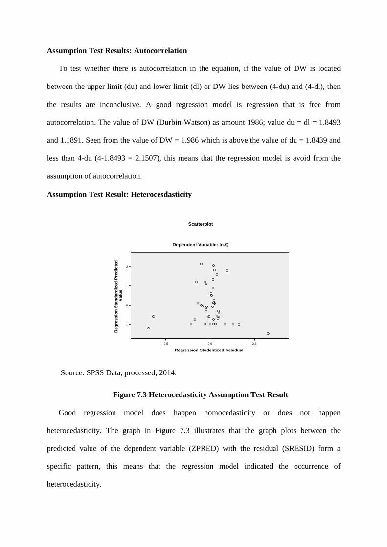
Assumption Test Result: Heterocesdasticity
Source: SPSS Data, processed, 2014.
Figure 7.3 Heterocedasticity Assumption Test Result
Good regression model does happen homocedasticity or does not happen
heterocedasticity. The graph in Figure 7.3 illustrates that the graph plots between the
predicted value of the dependent variable (ZPRED) with the residual (SRESID) form a
specific pattern, this means that the regression model indicated the occurrence of
heterocedasticity.
2.50.0-2.5
Regression Studentized Residual
2
1
0
-1
Reg
ressio
n S
tan
dard
ized
Pre
dic
ted
V
alu
e
Scatterplot
Dependent Variable: ln.Q

To avoid heteroscedasticity then doing further testing by using Park method. A good
regression model does not happen heterocedasticity. This test is performed to create a model
of regression between the value of absolute variance (Ui) as the dependent variable with the
independent variable (Gozali, 2001). If all independent variables are statistically significant
in the regression are the symptoms of heterocedasticity (Hasan, 1999), or if all the
independent variables were not statistically significant in the regression model did not occur
heterocedasticity. The results of the heterocedasticity test analysis by the Park method can be
seen in the appendix with the following results:
Table 7.4
Heterocesdasticity Assumption Test with Park Test Result
Source: Data processed, 2014.
Description:
X1 : Price of Chili
X2 : Price of Substitution Good
X3 : Price of Complementary Good
Coefficients a
-287.799 212.218 -1.356 .193
.083 .547 .046 .152 .881 -.048 .508 -.021 -.095 .925
-1.512 .595 -.742 -2.540 .071 26.303 17.818 .530 1.476 .158 -1.056 .635 -.414 -1.662 .115 -.076 .506 -.068 -.151 .882
(Constant) ln.x1
ln.x2 ln.x3 ln.x4 ln.x5 ln.x6
Model 1
B Std. Error
Unstandardized Coefficients
Beta
Standardized Coefficients
t Sig.
Dependent Variable: Ln.U2i a.
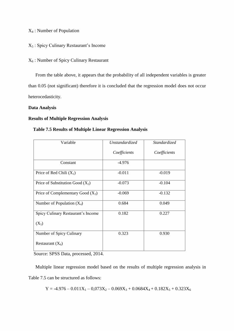
X4 : Number of Population
X5 : Spicy Culinary Restaurant’s Income
X6 : Number of Spicy Culinary Restaurant
From the table above, it appears that the probability of all independent variables is greater
than 0.05 (not significant) therefore it is concluded that the regression model does not occur
heterocedasticity.
Data Analysis
Results of Multiple Regression Analysis
Table 7.5 Results of Multiple Linear Regression Analysis
Variable Unstandardized
Coefficients
Standardized
Coefficients
Constant -4.976
Price of Red Chili (X1) -0.011 -0.019
Price of Substitution Good (X2) -0.073 -0.104
Price of Complementary Good (X3) -0.069 -0.132
Number of Population (X4) 0.684 0.049
Spicy Culinary Restaurant’s Income
(X5)
0.182 0.227
Number of Spicy Culinary
Restaurant (X6)
0.323 0.930
Source: SPSS Data, processed, 2014.
Multiple linear regression model based on the results of multiple regression analysis in
Table 7.5 can be structured as follows:
Y = -4.976 – 0.011X1 – 0,073X2 – 0.069X3 + 0.0684X4 + 0.182X5 + 0.323X6

From the regression model analysis, it is aimed to know the influence Price of Red Chili
(X1), Price of Substitution Good (X2), Price of Complementary Good (X3) cause the
decreasing on Demand (Y). That is, if an increase in (X1), (X2), (X3) then it will lead to a
decrease in demand (Y). Conversely, if there is a decrease in (X1), (X2), and (X3) there will
be an increase on demand (Y).
For variable Number of Population (X4), Spicy Culinary Restaurant Income (X5), and
Number of Spicy Culinary Restaurant (X6) have a positive influence on demand (Y), means
that if there is an increase on (X4), (X5) , and (X6) the demand (Y) will also increase.
Conversely, if there is a decrease in (X4), (X5), and (X6) then it will be followed by
decreasing on demand (Y).
Multiple Correlation Analysis
In regression analysis result, the correlation or relationship between variables will be
known. Multiple correlation analysis is used to determine the relationship between variables.
Table 7.6 Correlation Analysis Result
Dependent Variable Independent Variables R R square
Demand (Y)
Price of Red Chili (X1)
0.953 0.909
Price of Substitution Good
(X2)
Price of Complementary
Good (X3)
Number of Population (X4)
Spicy Culinary Restaurant’s
Income (X5)
Number of Spicy Culinary
Restaurant (X6)
Source: SPSS Data processed, 2014.
Description:
R : Multiple correlation coefficient
R2 : Determination coefficient
Correlation between all independent variables on the dependent variable can be seen from
coefficients R. The tight measurements are:
0 – 0.2 : Very weak
0.2 – 0.4 : Weak
0.4 – 0.6 : Quite
0.6 – 0.8 : Strong
0.8 – 1 > Very strong
Known coefficient R as amount of 0.953, which means the relationship between all the
independent variables on the dependent variable are strong.
Based on the results of the calculation which presented in Table 7.6 value of R2
obtained as amount 0.909 this means that the variable (X1), (X2), (X3), Number of Population
(X4), (X5), (X6) simultaneously explain 90.9% variation in the magnitude of change in
demand (Y), while another change in demand (Y) is influenced by other variables which is
not examined in the amount of 9.1%.
8.Hypothesis Testing
As expected Price of Red Chili (X1), Price of Substitution Good (X2), Price of
Complementary Good (X3), Number of Population (X4), Spicy Culinary Restaurant's
IncomeS (X5), and Number of Spicy Culinary Restaurant (X6) simultaneously effect on
Demand (Y).
To test the hypothesis the F test is used, which is to test statistically whether the
independent variables simultaneously have a significant effect on the dependent variable. The
F-test result are presented in the table below.
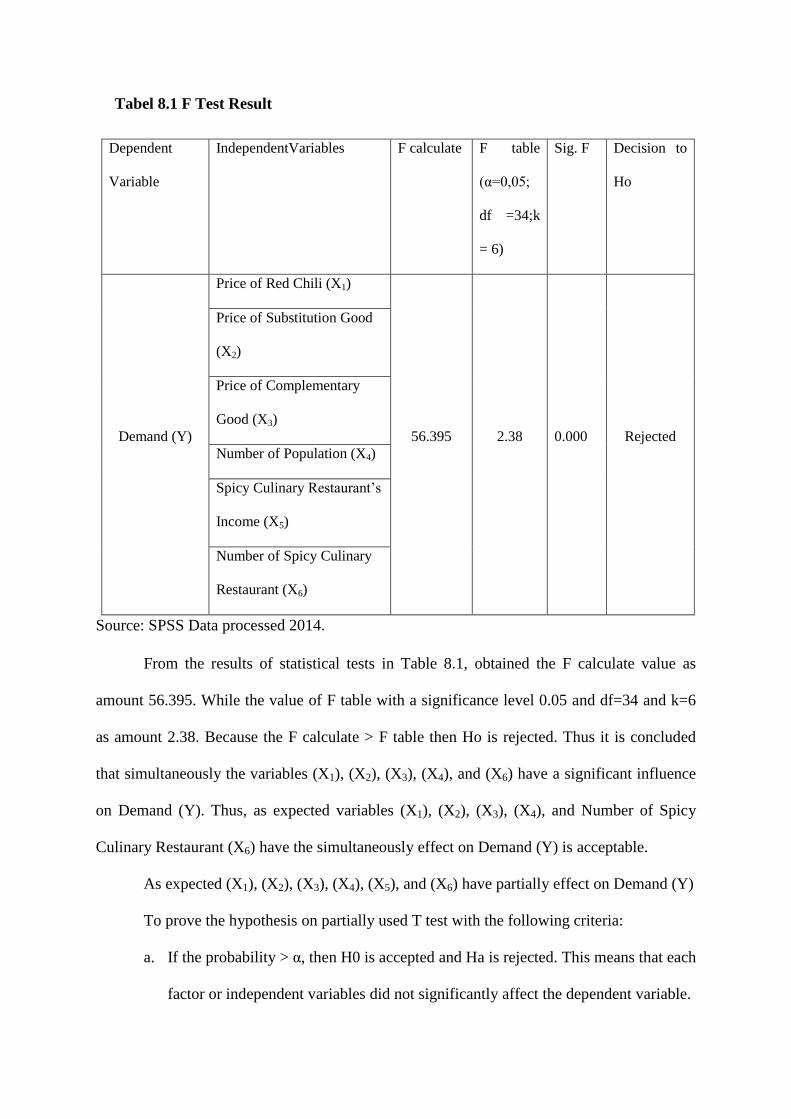
Tabel 8.1 F Test Result
Dependent
Variable
IndependentVariables F calculate F table
(α=0,05;
df =34;k
= 6)
Sig. F Decision to
Ho
Demand (Y)
Price of Red Chili (X1)
56.395 2.38 0.000 Rejected
Price of Substitution Good
(X2)
Price of Complementary
Good (X3)
Number of Population (X4)
Spicy Culinary Restaurant’s
Income (X5)
Number of Spicy Culinary
Restaurant (X6)
Source: SPSS Data processed 2014.
From the results of statistical tests in Table 8.1, obtained the F calculate value as
amount 56.395. While the value of F table with a significance level 0.05 and df=34 and k=6
as amount 2.38. Because the F calculate > F table then Ho is rejected. Thus it is concluded
that simultaneously the variables (X1), (X2), (X3), (X4), and (X6) have a significant influence
on Demand (Y). Thus, as expected variables (X1), (X2), (X3), (X4), and Number of Spicy
Culinary Restaurant (X6) have the simultaneously effect on Demand (Y) is acceptable.
As expected (X1), (X2), (X3), (X4), (X5), and (X6) have partially effect on Demand (Y)
To prove the hypothesis on partially used T test with the following criteria:
a. If the probability > α, then H0 is accepted and Ha is rejected. This means that each
factor or independent variables did not significantly affect the dependent variable.
b. If the probability is ≤ α, then H0 is rejected and Ha is accepted. This means that
each of the independent variables significantly affect to the dependent variable.
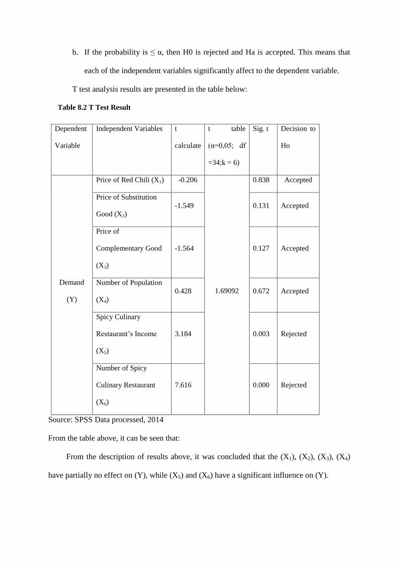
T test analysis results are presented in the table below:
Table 8.2 T Test Result
Dependent
Variable
Independent Variables t
calculate
t table
(α=0,05; df
=34;k = 6)
Sig. t Decision to
Ho
Demand
(Y)
Price of Red Chili (X1) -0.206
1.69092
0.838 Accepted
Price of Substitution
Good (X2)
-1.549 0.131 Accepted
Price of
Complementary Good
(X3)
-1.564 0.127 Accepted
Number of Population
(X4)
0.428 0.672 Accepted
Spicy Culinary
Restaurant’s Income
(X5)
3.184 0.003 Rejected
Number of Spicy
Culinary Restaurant
(X6)
7.616 0.000 Rejected
Source: SPSS Data processed, 2014
From the table above, it can be seen that:
From the description of results above, it was concluded that the (X1), (X2), (X3), (X4)
have partially no effect on (Y), while (X5) and (X6) have a significant influence on (Y).
Demand Elasticity
To test the level of sensitivity of demand to price changes can be seen by looking at the
regression coefficients of each independent variables. Because one of the interesting
characteristics of multiple logarithmic regression models that regression coefficient bi is the
value of its elasticity. So with this model, the value of its elasticity is the regression
coefficient of each independent variables, that occurred in the variables that had been studied
using income elasticity.
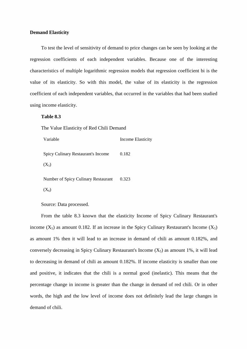
Table 8.3
The Value Elasticity of Red Chili Demand
Variable Income Elasticity
Spicy Culinary Restaurant's Income
(X5)
0.182
Number of Spicy Culinary Restaurant
(X6)
0.323
Source: Data processed.
From the table 8.3 known that the elasticity Income of Spicy Culinary Restaurant's
income (X5) as amount 0.182. If an increase in the Spicy Culinary Restaurant's Income (X5)
as amount 1% then it will lead to an increase in demand of chili as amount 0.182%, and
conversely decreasing in Spicy Culinary Restaurant's Income (X5) as amount 1%, it will lead
to decreasing in demand of chili as amount 0.182%. If income elasticity is smaller than one
and positive, it indicates that the chili is a normal good (inelastic). This means that the
percentage change in income is greater than the change in demand of red chili. Or in other
words, the high and the low level of income does not definitely lead the large changes in
demand of chili.
The table 8.3 known the elasticity income of the Number of Spicy Culinary Restaurant
(X6) as amount 0.323. If an increase in the Number of Spicy Culinary Restaurant (X6) as
amount as 1% then it will lead to an increase in demand of red chili as amount 0.323%, and
conversely decreasing the Number of Spicy Culinary Restaurant (X6) as amount 1%, it will
lead to decreasing in demand of red chili as amount 0.323%. Income elasticity is smaller than
one and positive indicates that the red chili is a normal good (inelastic). This means that the
percentage change in quantity of spicy restaurant is greater than the changes in demand of red
chili. Or in other words, the high and the low level of the number of spicy restaurant does not
definitely lead the large changes in demand of red chili.
9. Conclusion
1. From the partial analysis, concluded that :
a) The variable Spicy Culinary Restaurant’s Income (X5) were considered
significant to the demand of red chili (Y) the need of red chili as a
seasoning of food products is produce extremely large, thus requiring is
about 5 kg per day to produce the products that are offered, so the high
income of restaurant indicates the purchasing power of spicy food is very
high, that it is very influential on demand of red chili. The higher the
income of restaurant the greater the demand for red chili.
b) The variable Number of Spicy Culinary Restaurant (X6) were considered
significant to the demand of red chili (Y) because the increasing amount
of spicy culinary restaurant will stimulate the demand of red chili.
2. Price of red chili, price of substitution good, price of complementary good, number of
population, spicy culinary restaurant income, and number of spicy culinary restaurant
simultaneously have significant effect on demand of red chili.

3. Spicy culinary restaurant's income which has an income elasticity as amount 0.182 and
the number of spicy culinary restaurant has an income elasticity as amount 0.323. Those
mean that the high or low level of both spicy culinary restaurant’s income and spicy
culinary restaurant in Blimbing District do not lead the large change in demand of red
chili in the market.
4. There is the high cost in distribution of chili, because the farmers of chili only available
outside Blimbing District and also wheather and land condition affect the implantation of
chili. This supply push inflation cannot be solved with decreasing the amount of money
that have been spread, but can be solved with increasing productivity and developing the
sector of volatile and export goods in the local area that have prospect condition.
10. Suggestions
From the conclusions above, here is given a few suggestions that can be used as
consideration:
1. Every spicy culinary business should have to control the demand of commodities (red
chili, big red chili, and onion), then in running their business there would not be
inflation because of the demand of commodities is high without caring to the price of
commodities whether they are in high or low level.
2. Government participate to control the information of production from the local
farmers. Have cooperation in order to inform the potential time of implantation is
proper and prospect inside the demand of market and when is the implantation time
will be fall and scarce in the demand of market.

BIBLIOGRAPHY
Burhan, Umar. 2006. Konsep Dasar Teori Ekonomi Mikro. BPFE Unibraw . Malang.
Dewi, Tria Rosana, 2009, Analisis Permintaan Cabai Merah Di Surakarta. Minor Thesis,
Faculty of Agriculture, Sebelas Maret University, Surakarta, (online), accessed on
April 1st,
2014.
Ghozali, Imam. 2001. Aplikasi Analisis Multivariate Dengan Program SPSS 2nd
edition.
Badan Penerbit Universitas Diponegoro. Semarang.
Given, Lisa M. (editor). 2008. The Sage Encyclopedia of Qualitative Research Methods.
Thousand Oaks: Sage.
Nazir, M. 2003. Metode Penelitian. Ghalia Indonesia. Jakarta.
Pappas, J.L dan M. Hirschey. 1995. Ekonomi Manajerial Jilid 1. Binarupa Aksara. Jakarta.
Sukirno, Sadono. 2003. Pengantar Teori Mikroekonomi 1st edition. PT Raja Grafindo
Persada. Jakarta.
Tjiptono, Fandy. 2008. Strategi Pemasaran 3rd
edition. Andy. Yogyakarta.